HYDROGEN Ly� INTENSITY OSCILLATIONS OBSERVED BY THE SOLAR AND HELIOSPHERICOBSERVATORY ULTRAVIOLET CORONAGRAPH SPECTROMETER

H. Morgan, S. Rifai Habbal,1and X. Li

Sefydliad y Gwyddorau Mathemategol a Ffisegol, Prifysgol Cymru, Aberystwyth, Ceredigion, Cymru SY23 3BZ, UK; hhm01@aber.ac.uk

Received 2003 September 16; accepted 2003 December 22

ABSTRACT

We report on a search for significant oscillations in different coronal structures by applying a wavelet analysisto Solar and Heliospheric Observatory UVCS observations of the hydrogen Ly� 1216 8 line intensity takenbetween 1.5 and 2.2 R�. Significant periodic oscillations, unlikely to be a result of instrumental effects, areshown to exist in a coronal hole, the quiet Sun, and a streamer. Observations made sequentially at differentheights but at the same latitude often share similar power spectra. Neighboring pixels at the same radial distancealso share similar power spectra. These results indicate both a localized structure to the periodicity and a long-range preservation of oscillation patterns in the radial expansion of the solar wind. We show that a preference forsignificant oscillations with periods of 7–8 minutes exists in three out of the four observations presented here.Other bands of preferred periodicity are observed at different heights.

Subject headings: Sun: corona — Sun: oscillations — Sun: UV radiation

1. INTRODUCTION

The study of oscillations in ion intensity in the chromo-sphere and off-limb atmosphere is a well-established field, andthere exists a large body of literature on results from instru-ments such as TRACE (Rutten & Krijger 2003; McIntosh,Fleck, & Judge 2003; Muglach 2003) and the Solar andHeliospheric Observatory (SOHO) SUMER (Wang et al.2003) and CDS (Marsh et al. 2003; Banerjee et al. 2001), tolist but a few recent studies. The high intensities of emissionlines close to the Sun enable these instruments to acquire dataat a high temporal resolution with a reasonable signal-to-noiseratio. Observations by the SOHO/UVCS starting at 1.5 R� areless well suited for temporal analysis, and the problems posedby a low signal-to-noise ratio, particularly at larger heliocentricdistances in nonstreamer regions, are considerable. Temporalstudies of UVCS emission-line observations at the highestobservational frequencies are therefore rare, although detailedstudies of oscillations in polarized brightness from the UVCSwhite-light channel have been made (Ofman et al. 1997, 2000).

Standard spectroscopic analysis of UVCS data involves in-tegrating photon counts over many exposures. Combiningmany short exposures lessens Poisson uncertainties in photoncounts and produces spectral profiles that easily accommodatefitting to Gaussian functions. In this paper we make no attemptto use this standard approach to the data. Preservation of thesignal at the highest spatial and temporal resolution forces theuse of raw photon counts with a minimum of preprocessing.Wavelet analysis is applied to the data, and an appropriate testis employed that reveals the presence of significant oscil-lations. The method is applied to a set of UVCS observationsof hydrogen Ly� taken in 2002 June at a range of heightsabove the south polar region and southeast midlatitudestreamers. A description of the observations is given in x 2, theanalysis techniques are explained in x 3, and results are pre-sented in x 4, followed by a discussion in x 5 and concludingremarks in x 6.

2. OBSERVATIONS

The spectroscopic observations of the hydrogen Ly� linepresented in this paper were obtained using the redundant Ly�channel on the UVCS O vi detector on 2002 June 20–21. From23:00 on June 20 until 06:00 on June 21, the position angle ofthe UVCS slit center was 150� counterclockwise from north.Data were collected sequentially at heights of 2.0, 2.2, 1.8, and1.5 R� during the 7 hours of observations. Table 1 gives thestart and end times and number of exposures for each heightobserved. For these observations, there are 60 spatial binsalong the UVCS slit, giving a minimum spatial resolution of4200. Each observation has an average time of 130 s betweenexposures.

Figure 1 (left) shows a UVCS/LASCO C2 and UVCS/EITcomposite image of the southeastern corona from June 21,with lines drawn to indicate the different slit positions. The slitextends from above the south pole to across the midlatitudestreamers at �150�. Note that the streamers are partially ob-scured near 135� in the figure because of the mount of theLASCO occulting disk. Low-resolution Kitt Peak coronal-hole maps indicate the presence of a coronal hole over thesouth pole during the time of the observations. Although 2002June was a time of considerable activity in the solar corona,the data in this paper were not affected by coronal massejection activity. The midlatitude streamers remained stablethroughout the 7 hours of observations, with some slowmovement due to solar rotation.

Intensity is obtained at all four slit heights from the time-integrated Ly� profiles using the standard UVCS analysissoftware package, DAS33. Figure 1 (right) is constructedfrom interpolating between the log of intensity at all heightsobserved. Fitting errors are avoided, and the signal-to-noiseratio is greatly improved by employing a sliding window of 5slit pixels. Cubic convolution is used to interpolate for theheights between the slits. The observed heights are shown bythe horizontal lines in Figure 1 (right), while lines of constantlatitude are shown by the dashed lines. The vertical axisdenotes the heliocentric height at a latitude of 150�, and thehorizontal axis denotes the latitude for the 1.5 R� observation.

1 Also at Harvard-Smithsonian Center for Astrophysics, 60 Garden Street,Cambridge, MA 02138.

521

The Astrophysical Journal, 605:521–527, 2004 April 10

# 2004. The American Astronomical Society. All rights reserved. Printed in U.S.A.

It is not an easy or exact matter to identify structures in thecorona from UVCS data because of the sharp intrinsic drop ofintensity with height. However, from the LASCO C2 image inFigure 1 (left), the daily LASCO C2 movie, the Kitt Peakcoronal-hole map, and Figure 1 (right), we have identified andlabeled three distinct regions covered by the UVCS slit inthese observations. The streamer is most easily identified asthe region of high intensity, labeled ‘‘S’’ and bounded bywhite lines in Figure 1 (right). We can see two intensity peaksin the streamer, one lying approximately radially at �143� andthe other varying in latitude from 128� to 134� with increasingheight. The coronal hole, labeled ‘‘C,’’ is identified by thedrop in intensity, which varies in latitude from just under180� at 1.5 R� to 172� at 2.2 R�. An area between thestreamer and coronal hole, labeled ‘‘Q,’’ is identified with thequiet Sun, with smoothly decreasing intensity with increasinglatitude.

3. DATA ANALYSIS

The nature of our search for significant oscillations inUVCS data allows us to disregard many standard techniquesusually associated with the instrument. Since we are interestedonly in relative temporal fluctuations of intensity, we ignoreinstrumental influences on the line profile and intensity that

remain constant in time, such as the slit profile deconvolutionand detector flat-field correction. We make no estimated cor-rection for stray light or light from interplanetary hydrogen,under the assumption that these unwanted contributionschange only slowly.The Ly� 1216 8 line is identified in the appropriate UVCS

detector mask, and the photon counts are integrated over thewavelength range of the line. Since the position and width ofthe Ly� line on the detector can vary because of physical andinstrumental causes, we estimate the appropriate wavelengthrange separately for each pixel along the slit. The range isestimated from the mean wavelength and line width of thetime-integrated line profile for that pixel. The few unreliablespatial pixels at the extremities of the UVCS slit are discarded.After integrating over the line profile, we obtain a time

series of Ly� photon counts for each UVCS pixel along theslit. The exposure time for these observations is a constant120 s. There is, however, a pause of approximately 10 s be-tween each exposure, a pause that can vary by a second or twothroughout an observation. The cadence is therefore �130 s,with data being collected for only 120 of each 130 s time step.Since the pauses between exposures are small compared to thecadence (<10%), we simply extrapolate by assuming a countrate during the pause equal to the preceding exposure. Since

TABLE 1

Details of the UVCS Observations

Height

(R�) Start Date Start Time End Date End Time Exposures

2.0........................ 2002 Jun 20 23:00 2002 Jun 21 01:01 56

2.2........................ 2002 Jun 21 01:02 2002 Jun 21 03:21 64

1.8........................ 2002 Jun 21 03:21 2002 Jun 21 04:48 40

1.5........................ 2002 Jun 21 04:49 2002 Jun 21 05:58 32

Fig. 1.—Left: Composite LASCO C2 and EIT image from June 21. Solid white lines indicate positions of the UVCS slit. Dotted white lines indicate latitude.Right: Ly� intensity interpolated into a contour plot of the observed region. Streamer, quiet-Sun, and coronal-hole regions are labeled ‘‘S,’’ ‘‘Q,’’ and ‘‘C’’ and arebounded by the white lines. The dashed lines are lines of constant latitude. Higher intensities have lighter shading. The intensity contours start at log1011:3 photonss�1 ��1 cm�2 8�1 at the lowest height and decrease by log100:065 photons s�1 ��1 cm�2 8�1.

MORGAN, HABBAL, & LI522 Vol. 605

the variance in pause time between exposures is very smallcompared to the total exposure time (<1%), no attempt ismade to interpolate to a constant time step; we take the av-erage time step (�130 s) as a constant for the whole obser-vation. The uncertainties in photon counts rising from the gapsin observation are unavoidable but acceptable. The uncer-tainties due to the varying time steps are negligible.

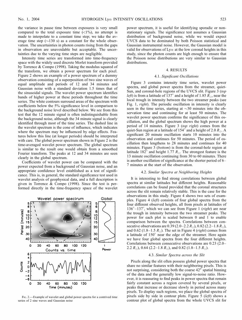
Intensity time series are transformed into time-frequencyspace with the widely used discrete Morlet transform providedby Torrence & Compo (1998). Taking the modulus squared ofthe transform, we obtain a power spectrum for each pixel.Figure 2 shows an example of a power spectrum of a dummyobservation consisting of a superposition of two sine waves ofequal amplitude and periods of 12 and 34 minutes andGaussian noise with a standard deviation 1.5 times that ofthe sinusoidal signals. The wavelet power spectrum identifiesbands of higher power at these periods throughout the timeseries. The white contours surround areas of the spectrum withcoefficients below the 5% significance level in comparison tothe background noise level described below. We see from thistest that the 12 minute signal is often indistinguishable fromthe background noise, although the 34 minute signal is clearlyidentified through most of the time series. The dashed line inthe wavelet spectrum is the cone of influence, which indicateswhere the spectrum may be influenced by edge effects. Fea-tures below this line (at longer periods) should be interpretedwith care. The global power spectrum shown in Figure 2 is thetime-averaged wavelet power spectrum. The global spectrumis similar to the result one would obtain from a smoothedFourier transform. The peaks at 12 and 34 minutes are seenclearly in the global spectrum.

Coefficients of wavelet power can be compared with thepower expected from a background of Gaussian noise, and anappropriate confidence level established as a test of signifi-cance. This is, in general, the standard significance test used inwavelet analysis of geophysical data, and a full description isgiven in Torrence & Compo (1998). Since the test is per-formed directly in the time-frequency space of the wavelet

power spectrum, it is useful for identifying sporadic or non-stationary signals. The significance test assumes a Gaussiandistribution of background noise, while we would expectUVCS data to be dominated by both Poisson statistical andGaussian instrumental noise. However, the Gaussian model isvalid for observations of Ly� at the low coronal heights in thisstudy, since the photon counts are high enough to ensure thatthe Poisson noise distributions are very similar to Gaussiandistributions.

4. RESULTS

4.1. Significant Oscillations

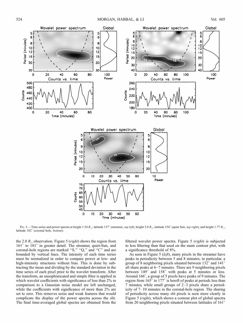
Figure 3 contains intensity time series, wavelet powerspectra, and global power spectra from the streamer, quiet-Sun, and coronal-hole regions of the UVCS slit. Figure 3 (topleft) is from a latitude of 137� and a height of 1.85 R�, near thelocal trough in intensity between the two streamer peaks (seeFig. 1, right). The periodic oscillation in intensity is clearlyseen in the time series, starting at �30 minutes into the ob-servation time and continuing for at least 50 minutes. Thewavelet power spectrum confirms the significance of this os-cillation, and the global spectrum shows the high power at aperiod of 14 minutes. Figure 3 (top right) comes from thequiet-Sun region at a latitude of 154� and a height of 2.0 R�. Asignificant 20 minute oscillation starts 10 minutes into theobservation and continues for 50 minutes. The period of os-cillation then lengthens to 28 minutes and continues for 40minutes. Figure 3 (bottom) is from the coronal-hole region atlatitude 182� and height 1.77 R�. The strongest feature is the13 minute oscillation continuing from 30 to 60 minutes. Thereis another oscillation of significance at the shorter period of 6–7 minutes at the start of the observation.

4.2. Similar Spectra at Neighboring Heights

It is interesting to find strong correlations between globalspectra at similar latitudes but different heights. Reasonablecorrelations can be found provided that the coronal structuresacross the slit remain relatively stable. This is the case for theobservations in this study. Figure 4 shows two sets of exam-ples. Figure 4 (left) consists of four global spectra from thefour different observed heights, all from pixels at latitudes of136�–137�, which we can see from Figure 1 (right) are nearthe trough in intensity between the two streamer peaks. Thepower for each plot is scaled between 0 and 1 to enablecomparison between the spectra. Correlations between con-secutive observations are 0.39 (2.0–2.2 R�), 0.82 (2.2–1.8 R�),and 0.62 (1.8–1.5 R�). The set in Figure 4 (right) comes froma latitude of 150� near the edge of the streamer. Here againwe have four global spectra from the four different heights.Correlations between consecutive observations are 0.23 (2.0–2.2 R�), 0.64 (2.2–1.8 R�), and 0.82 (1.8–1.5 R�).

4.3. Similar Spectra across the Slit

Pixels along the slit often possess global power spectra thatshare no similar features with their neighboring pixels. This isnot surprising, considering both the coarse 4200 spatial binningof the data and the generally low signal-to-noise ratio. How-ever, it is reassuring to find peaks in power spectra that remainfairly constant across a region covered by several pixels, orpeaks that increase or decrease slowly in period across manypixels. To display such regions, we place the global spectra ofpixels side by side in contour plots. Figure 5 (left) shows acontour plot of global spectra from the whole UVCS slit for

Fig. 2.—Example of wavelet and global power spectra for a contrived timeseries of 2 sine waves and Gaussian noise

HYDROGEN Ly� INTENSITY OSCILLATIONS 523No. 1, 2004

the 2.0 R� observation. Figure 5 (right) shows the region from161� to 181� in greater detail. The streamer, quiet-Sun, andcoronal-hole regions are marked ‘‘S,’’ ‘‘Q,’’ and ‘‘C’’ and arebounded by vertical lines. The intensity of each time seriesmust be normalized in order to compare power at low- andhigh-intensity structures without bias. This is done by sub-tracting the mean and dividing by the standard deviation in thetime series of each pixel prior to the wavelet transform. Afterthe transform, an unsophisticated and simple filter is applied inwhich wavelet coefficients with significance of less than 2% incomparison to a Gaussian noise model are left unchanged,while the coefficients with significance of more than 2% areset to zero. This removes noise and weak features that wouldcomplicate the display of the power spectra across the slit.The final time-averaged global spectra are obtained from the

filtered wavelet power spectra. Figure 5 (right) is subjectedto less filtering than that used on the main contour plot, witha significance threshold of 8%.As seen in Figure 5 (left), many pixels in the streamer have

peaks in periodicity between 5 and 8 minutes; in particular, agroup of 8 neighboring pixels situated between 132� and 141�

all share peaks at 6–7 minutes. There are 9 neighboring pixelsbetween 149

�and 158

�with peaks at 5 minutes or less.

Around 166�, a group of 5 pixels have peaks of 9 minutes. Theregion from 165� to 177� is bereft of peaks at periods less than7 minutes, while small groups of 2–3 pixels share a period-icity of 7–10 minutes in the coronal-hole region. The sharingof periodicity across many slit pixels is seen more clearly inFigure 5 (right), which shows a contour plot of global spectrafrom 20 neighboring pixels situated between latitudes of 161

�

Fig. 3.—Time series and power spectra at height 1.54 R�, latitude 137� (streamer, top left), height 2.0 R�, latitude 154

� (quiet Sun, top right), and height 1.77 R�,latitude 182� (coronal hole, bottom).

MORGAN, HABBAL, & LI524 Vol. 605

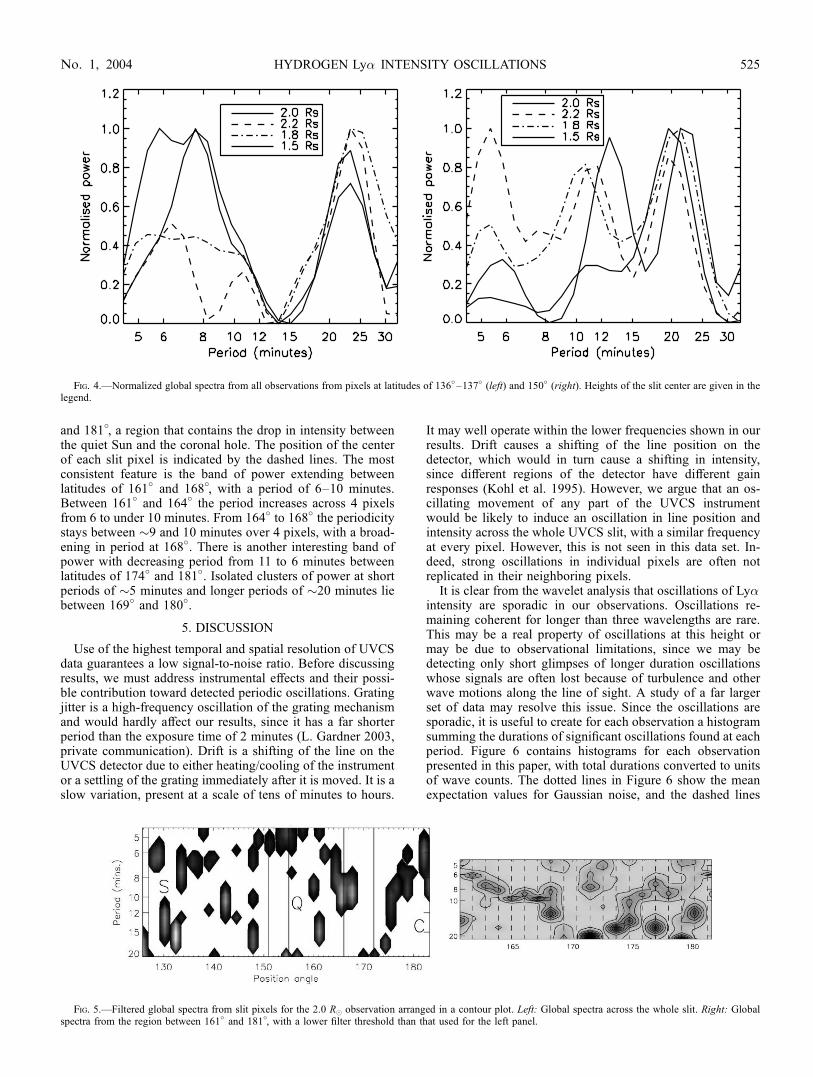
and 181�, a region that contains the drop in intensity betweenthe quiet Sun and the coronal hole. The position of the centerof each slit pixel is indicated by the dashed lines. The mostconsistent feature is the band of power extending betweenlatitudes of 161

�and 168

�, with a period of 6–10 minutes.

Between 161�and 164

�the period increases across 4 pixels

from 6 to under 10 minutes. From 164� to 168� the periodicitystays between �9 and 10 minutes over 4 pixels, with a broad-ening in period at 168

�. There is another interesting band of

power with decreasing period from 11 to 6 minutes betweenlatitudes of 174� and 181�. Isolated clusters of power at shortperiods of �5 minutes and longer periods of �20 minutes liebetween 169� and 180�.

5. DISCUSSION

Use of the highest temporal and spatial resolution of UVCSdata guarantees a low signal-to-noise ratio. Before discussingresults, we must address instrumental effects and their possi-ble contribution toward detected periodic oscillations. Gratingjitter is a high-frequency oscillation of the grating mechanismand would hardly affect our results, since it has a far shorterperiod than the exposure time of 2 minutes (L. Gardner 2003,private communication). Drift is a shifting of the line on theUVCS detector due to either heating/cooling of the instrumentor a settling of the grating immediately after it is moved. It is aslow variation, present at a scale of tens of minutes to hours.

It may well operate within the lower frequencies shown in ourresults. Drift causes a shifting of the line position on thedetector, which would in turn cause a shifting in intensity,since different regions of the detector have different gainresponses (Kohl et al. 1995). However, we argue that an os-cillating movement of any part of the UVCS instrumentwould be likely to induce an oscillation in line position andintensity across the whole UVCS slit, with a similar frequencyat every pixel. However, this is not seen in this data set. In-deed, strong oscillations in individual pixels are often notreplicated in their neighboring pixels.

It is clear from the wavelet analysis that oscillations of Ly�intensity are sporadic in our observations. Oscillations re-maining coherent for longer than three wavelengths are rare.This may be a real property of oscillations at this height ormay be due to observational limitations, since we may bedetecting only short glimpses of longer duration oscillationswhose signals are often lost because of turbulence and otherwave motions along the line of sight. A study of a far largerset of data may resolve this issue. Since the oscillations aresporadic, it is useful to create for each observation a histogramsumming the durations of significant oscillations found at eachperiod. Figure 6 contains histograms for each observationpresented in this paper, with total durations converted to unitsof wave counts. The dotted lines in Figure 6 show the meanexpectation values for Gaussian noise, and the dashed lines

Fig. 4.—Normalized global spectra from all observations from pixels at latitudes of 136�–137� (left) and 150� (right). Heights of the slit center are given in thelegend.

Fig. 5.—Filtered global spectra from slit pixels for the 2.0 R� observation arranged in a contour plot. Left: Global spectra across the whole slit. Right: Globalspectra from the region between 161

�and 181

�, with a lower filter threshold than that used for the left panel.

HYDROGEN Ly� INTENSITY OSCILLATIONS 525No. 1, 2004

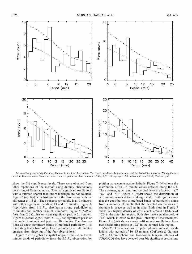
show the 5% significance levels. These were obtained from2000 repetitions of the method using dummy observationsconsisting of Gaussian noise. Note that significant oscillationswith a duration shorter than one wavelength are not counted.Figure 6 (top left) is the histogram for the observation with theslit center at 1.5 R�. The strongest periodicity is at 8 minutes,with other significant bands at 13 and 16 minutes. Figure 6(top right), from 1.8 R�, also has a strong periodicity at8 minutes and another band at 5 minutes. Figure 6 (bottomleft), from 2.0 R�, has only one significant peak at 21 minutes.Figure 6 (bottom right), from 2.2 R�, has significant peaks atjust under 8 minutes and just over 10 minutes. The observa-tions all show significant bands of preferred periodicity. It isinteresting that a band of preferred periodicity of �8 minutesemerges from three out of the four observations.

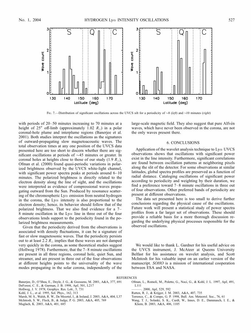
Figure 7 investigates the spatial origin of the �8 and �10minute bands of periodicity from the 2.2 R� observation by

plotting wave counts against latitude. Figure 7 (left) shows thedistribution of all �8 minute waves detected along the slit.The streamer, quiet Sun, and coronal hole are labeled ‘‘S,’’‘‘Q,’’ and ‘‘C.’’ Figure 7 (right) shows the distribution of�10 minute waves detected along the slit. Both figures showthat the contributions to preferred bands of periodicity comefrom a minority of pixels: that the detected oscillations aresporadic in space as well as in time. Both plots in Figure 7show their highest density of wave counts around a latitude of162� in the quiet-Sun region. Both also have a smaller peak at142

�, which is close to the peak intensity of the streamers.

Figure 7 (right) shows strong �10 minute oscillations fromtwo neighboring pixels at 172� in the coronal-hole region.SOHO/EIT observations of polar plumes indicate oscil-

lations with periods of 10–15 minutes (DeForest & Gurman1998). Chromospheric and low-corona temporal studies ofSOHO/CDS data have detected possible significant oscillations

Fig. 6.—Histograms of significant oscillations for the four observations. The dotted line shows the mean value, and the dashed line shows the 5% significancelevel for Gaussian noise. Shown are wave count vs. period for observations at 1.5 (top left), 1.8 (top right), 2.0 (bottom left), and 2.2 R� (bottom right).

MORGAN, HABBAL, & LI526 Vol. 605

with periods of 20–50 minutes increasing to 70 minutes at aheight of 2500 off-limb (approximately 1.02 R�) in a polarcoronal-hole plume and interplume regions (Banerjee et al.2001). Both studies interpret the oscillations as the signaturesof outward-propagating slow magnetoacoustic waves. Thetotal observation times at any one position of the UVCS datapresented here are too short to discern whether there are sig-nificant oscillations at periods of �45 minutes or greater. Incoronal holes at heights close to those of our study (1.9 R�),Ofman et al. (2000) found quasi-periodic variations in polar-ized brightness observed by the UVCS white-light channel,with significant power spectra peaks at periods around 6–10minutes. The polarized brightness is directly related to theelectron density along the line of sight, and the oscillationswere interpreted as evidence of compressional waves propa-gating outward from the Sun. Produced by resonance scatter-ing of the chromospheric Ly� emission from neutral hydrogenin the corona, the Ly� intensity is also proportional to theelectron density; hence, its behavior should follow that of thepolarized brightness. That we also find evidence for a 7–8 minute oscillation in the Ly� line in three out of the fourobservations lends support to the periodicity found in the po-larized brightness measurements.

Given that the periodicity derived from the observations isassociated with density fluctuations, it can be a signature offast or slow magnetosonic waves. That the periodicity persistsout to at least 2.2 R� implies that these waves are not dampedvery quickly in the corona, as some theoretical studies suggest(Hollweg 1978). Furthermore, that the 7–8 minute oscillationsare present in all three regions, coronal hole, quiet Sun, andstreamer, and are present in three out of the four observationsat different heights points to the universality of the wavemodes propagating in the solar corona, independently of the

large-scale magnetic field. They also suggest that pure Alfvenwaves, which have never been observed in the corona, are notthe only waves present there.

6. CONCLUSIONS

Application of the wavelet analysis technique to Ly� UVCSobservations shows that oscillations with significant powerexist in the line intensity. Furthermore, significant correlationsare found between oscillation patterns at neighboring pixelsalong the slit of the detector. For some observations at similarlatitudes, global spectra profiles are preserved as a function ofradial distance. Cataloging oscillations of significant poweraccording to periodicity and weighting by their duration, wefind a preference toward 7–8 minute oscillations in three outof four observations. Other preferred bands of periodicity arepresent at different observations.

The data set presented here is too small to derive furtherconclusions regarding the physical cause of the oscillations.Future work will present a statistical study of power spectraprofiles from a far larger set of observations. These shouldprovide a reliable basis for a more thorough discussion re-garding the underlying physical processes responsible for theobserved oscillations.

We would like to thank L. Gardner for his useful advice onthe UVCS instrument, J. McAteer at Queens UniversityBelfast for his assistance on wavelet analysis, and ScottMcIntosh for his valuable input on an earlier version of themanuscript. SOHO is a mission of international cooperationbetween ESA and NASA.

REFERENCES

Banerjee, D., O’Shea, E., Doyle, J. G., & Goossens, M. 2001, A&A, 377, 691DeForest, C. E., & Gurman, J. B. 1998, ApJ, 501, L217Hollweg, J. V. 1978, Geophys. Res. Lett., 5, 731Kohl, J. L., et al. 1995, Sol. Phys., 162, 313Marsh, M. S., Walsh, R. W., De Moortel, I., & Ireland, J. 2003, A&A, 404, L37McIntosh, S. W., Fleck, B., & Judge, P. G. 2003, A&A, 405, 769Muglach, K. 2003, A&A, 401, 685

Ofman, L., Romoli, M., Poletto, G., Noci, G., & Kohl, J. L. 1997, ApJ, 491,L111

———. 2000, ApJ, 529, 592Rutten, R. J., & Krijger, J. M. 2003, A&A, 407, 735Torrence, C., & Compo, G. P. 1998, Bull. Am. Meteorol. Soc., 76, 61Wang, T. J., Solanki, S. K., Curdt, W., Innes, D. E., Dammasch, I. E., &Kliem, B. 2003, A&A, 406, 1105

Fig. 7.—Distribution of significant oscillations across the UVCS silt for a periodicity of �8 (left) and �10 minutes (right)

HYDROGEN Ly� INTENSITY OSCILLATIONS 527No. 1, 2004