CMS-TOTEM Precision Proton Spectrometer Technical ...

CER

N-L

HC

C-2

014-

021

/TO

TEM

-TD

R-0

0325

/09/

2014

TOTEM-TDR-003 CMS-TDR-13

CERN-LHCC-2014-021

September 8, 2014

CMS-TOTEM Precision Proton SpectrometerTechnical Design Report

The CMS and TOTEM Collaborations

Abstract

This report describes the technical design and outlines the expected performance of the CMS-TOTEM Precision Proton Spectrometer (CT-PPS). CT-PPS adds precision proton tracking and timingdetectors in the very forward region on both sides of CMS at about 200m from the IP to study centralexclusive production (CEP) in proton-proton collisions. CEP provides a unique method to access avariety of physics topics at high luminosity LHC, such as new physics via anomalous production ofW and Z boson pairs, high-pT jet production, and possibly the production of new resonances. TheCT-PPS detector consists of a silicon tracking system to measure the position and direction of theprotons, and a set of timing counters to measure their arrival time with a precision of the order of10 ps. This in turn allows the reconstruction of the mass and momentum as well as of the z coor-dinate of the primary vertex of the centrally produced system. The framework for the developmentand exploitation of CT-PPS is defined in a Memorandum of Understanding signed by CERN as thehost laboratory and the CMS and TOTEM Collaborations. The expected performance of CT-PPS isdiscussed, including detailed studies of exclusive WW and dijet production. The planning for theimplementation of the new detectors is presented, including construction, testing, and installation.

Editors

Mike Albrow, Michele Arneodo, Valentina Avati, Joachim Baechler, Nicolo Cartiglia, Mario Deile,Michele Gallinaro, Jonathan Hollar, Maurizio Lo Vetere, Kenneth Osterberg, Nicola Turini, Joao Varela,Doug Wright.

i

Contents

1 Introduction 11.1 Overview of the CMS-TOTEM Precision Proton Spectrometer . . . . . . . . . . . . . . 1

1.1.1 CMS-TOTEM Memorandum of Understanding . . . . . . . . . . . . . . . . . . 21.1.2 Detectors and experimental conditions . . . . . . . . . . . . . . . . . . . . . . . 3

1.2 Physics with the CMS-TOTEM Precision Proton Spectrometers . . . . . . . . . . . . . 51.2.1 Introduction to physics with CT-PPS . . . . . . . . . . . . . . . . . . . . . . . . 51.2.2 Two-photon collisions . . . . . . . . . . . . . . . . . . . . . . . . . . . . . . . 61.2.3 Tests of Quantum Chromodynamics . . . . . . . . . . . . . . . . . . . . . . . . 71.2.4 Photoproduction . . . . . . . . . . . . . . . . . . . . . . . . . . . . . . . . . . 9

1.3 Strategy and running scenarios . . . . . . . . . . . . . . . . . . . . . . . . . . . . . . . 101.3.1 Exploratory phase . . . . . . . . . . . . . . . . . . . . . . . . . . . . . . . . . 101.3.2 Data production phase . . . . . . . . . . . . . . . . . . . . . . . . . . . . . . . 11

2 Detector and Physics Performance 152.1 Beam optics . . . . . . . . . . . . . . . . . . . . . . . . . . . . . . . . . . . . . . . . . 152.2 Simulated samples . . . . . . . . . . . . . . . . . . . . . . . . . . . . . . . . . . . . . 172.3 Detector acceptance and resolution: ξ, t . . . . . . . . . . . . . . . . . . . . . . . . . . 182.4 Detector acceptance and resolution: mass . . . . . . . . . . . . . . . . . . . . . . . . . 212.5 Timing detectors . . . . . . . . . . . . . . . . . . . . . . . . . . . . . . . . . . . . . . 252.6 Background: pp induced background . . . . . . . . . . . . . . . . . . . . . . . . . . . . 272.7 Roman Pot detector alignment . . . . . . . . . . . . . . . . . . . . . . . . . . . . . . . 282.8 Physics processes . . . . . . . . . . . . . . . . . . . . . . . . . . . . . . . . . . . . . . 30

2.8.1 Central exclusive dijet production . . . . . . . . . . . . . . . . . . . . . . . . . 302.8.2 Central exclusive WW production . . . . . . . . . . . . . . . . . . . . . . . . . 39

3 Beam Pockets 483.1 The Roman Pot system and collimators in the 200 m region of IP5 . . . . . . . . . . . . 483.2 New Roman Pots for timing detectors . . . . . . . . . . . . . . . . . . . . . . . . . . . 48

3.2.1 The mechanical tests of new Roman Pot cylinders . . . . . . . . . . . . . . . . . 513.3 The RF Shield for the box-shaped horizontal Roman Pots . . . . . . . . . . . . . . . . . 513.4 Interaction with the beam environment . . . . . . . . . . . . . . . . . . . . . . . . . . . 51

3.4.1 Experience from 2012 . . . . . . . . . . . . . . . . . . . . . . . . . . . . . . . 513.4.2 Impedance . . . . . . . . . . . . . . . . . . . . . . . . . . . . . . . . . . . . . 533.4.3 The RF test in the lab . . . . . . . . . . . . . . . . . . . . . . . . . . . . . . . . 573.4.4 Vacuum . . . . . . . . . . . . . . . . . . . . . . . . . . . . . . . . . . . . . . . 573.4.5 Generation of particle showers . . . . . . . . . . . . . . . . . . . . . . . . . . . 58

3.5 Interplay between Roman Pots and collimators . . . . . . . . . . . . . . . . . . . . . . 603.5.1 The new collimators TCL4 and TCL6 . . . . . . . . . . . . . . . . . . . . . . . 603.5.2 Optimisation of Roman Pot and collimator settings . . . . . . . . . . . . . . . . 61

3.6 Movable Beam-Pipe . . . . . . . . . . . . . . . . . . . . . . . . . . . . . . . . . . . . 623.6.1 Movable beam-pipe design considerations . . . . . . . . . . . . . . . . . . . . . 633.6.2 Impedance . . . . . . . . . . . . . . . . . . . . . . . . . . . . . . . . . . . . . 633.6.3 Thin window and material budget . . . . . . . . . . . . . . . . . . . . . . . . . 643.6.4 Mechanical deformation . . . . . . . . . . . . . . . . . . . . . . . . . . . . . . 653.6.5 Cost and prototype development . . . . . . . . . . . . . . . . . . . . . . . . . . 67

4 Tracking Detectors 704.1 Silicon sensors . . . . . . . . . . . . . . . . . . . . . . . . . . . . . . . . . . . . . . . 71

4.1.1 Baseline solution: 3D silicon sensors . . . . . . . . . . . . . . . . . . . . . . . 714.1.2 Alternative solutions: slim-edge planar sensors . . . . . . . . . . . . . . . . . . 74

ii

4.2 The readout system . . . . . . . . . . . . . . . . . . . . . . . . . . . . . . . . . . . . . 754.3 The detector assembly . . . . . . . . . . . . . . . . . . . . . . . . . . . . . . . . . . . 764.4 The cooling system . . . . . . . . . . . . . . . . . . . . . . . . . . . . . . . . . . . . . 78

5 Timing Detectors 825.1 Requirements on the timing detectors and strategy . . . . . . . . . . . . . . . . . . . . . 825.2 The baseline Quartic detector . . . . . . . . . . . . . . . . . . . . . . . . . . . . . . . . 84

5.2.1 Cherenkov detectors for timing . . . . . . . . . . . . . . . . . . . . . . . . . . 845.2.2 Quartic design for Roman pots, with L-bar geometry . . . . . . . . . . . . . . . 845.2.3 Photodetectors: Silicon photomultipliers . . . . . . . . . . . . . . . . . . . . . . 875.2.4 Integration with Roman Pots . . . . . . . . . . . . . . . . . . . . . . . . . . . . 875.2.5 Monitoring, alignment, and in situ calibration . . . . . . . . . . . . . . . . . . . 905.2.6 Monte Carlo (GEANT4) simulations . . . . . . . . . . . . . . . . . . . . . . . . 925.2.7 Beam tests . . . . . . . . . . . . . . . . . . . . . . . . . . . . . . . . . . . . . 935.2.8 Future developments . . . . . . . . . . . . . . . . . . . . . . . . . . . . . . . . 955.2.9 Costs and timescale . . . . . . . . . . . . . . . . . . . . . . . . . . . . . . . . . 955.2.10 Summary of Quartic detectors . . . . . . . . . . . . . . . . . . . . . . . . . . . 96

5.3 Gas Cherenkov detector . . . . . . . . . . . . . . . . . . . . . . . . . . . . . . . . . . . 965.4 Readout System of the Cherenkov Detectors . . . . . . . . . . . . . . . . . . . . . . . . 100

5.4.1 Requirements . . . . . . . . . . . . . . . . . . . . . . . . . . . . . . . . . . . . 1005.4.2 System design . . . . . . . . . . . . . . . . . . . . . . . . . . . . . . . . . . . 1015.4.3 Amplifier-discriminator NINO . . . . . . . . . . . . . . . . . . . . . . . . . . . 1025.4.4 Time-to-digital converter HPTDC . . . . . . . . . . . . . . . . . . . . . . . . . 103

5.5 Diamond detectors . . . . . . . . . . . . . . . . . . . . . . . . . . . . . . . . . . . . . 1065.6 Fast timing silicon detectors . . . . . . . . . . . . . . . . . . . . . . . . . . . . . . . . 107

5.6.1 Measurements . . . . . . . . . . . . . . . . . . . . . . . . . . . . . . . . . . . 1095.6.2 Radiation tolerance of UFSD . . . . . . . . . . . . . . . . . . . . . . . . . . . . 1105.6.3 Future developments . . . . . . . . . . . . . . . . . . . . . . . . . . . . . . . . 1115.6.4 3D silicon sensors . . . . . . . . . . . . . . . . . . . . . . . . . . . . . . . . . 112

5.7 Timing and Trigger Control . . . . . . . . . . . . . . . . . . . . . . . . . . . . . . . . . 1135.7.1 Reference Timing System (CMS) . . . . . . . . . . . . . . . . . . . . . . . . . 1135.7.2 Reference Timing System (TOTEM) . . . . . . . . . . . . . . . . . . . . . . . . 115

5.8 Plans and Schedule . . . . . . . . . . . . . . . . . . . . . . . . . . . . . . . . . . . . . 119

6 Trigger Strategy 122

7 Organization, Responsibilities and Cost 1257.1 Participating Institutes . . . . . . . . . . . . . . . . . . . . . . . . . . . . . . . . . . . 1257.2 Project organization . . . . . . . . . . . . . . . . . . . . . . . . . . . . . . . . . . . . . 126

7.2.1 Physics organization . . . . . . . . . . . . . . . . . . . . . . . . . . . . . . . . 1277.3 Responsibilities and resources . . . . . . . . . . . . . . . . . . . . . . . . . . . . . . . 1287.4 Planning and cost estimate . . . . . . . . . . . . . . . . . . . . . . . . . . . . . . . . . 130

7.4.1 Cost estimate of baseline detector . . . . . . . . . . . . . . . . . . . . . . . . . 1307.4.2 Objectives, plans and cost of R&D programme . . . . . . . . . . . . . . . . . . 1327.4.3 Expected funding and cost sharing . . . . . . . . . . . . . . . . . . . . . . . . . 133

iii

1 Introduction

1.1 Overview of the CMS-TOTEM Precision Proton Spectrometer

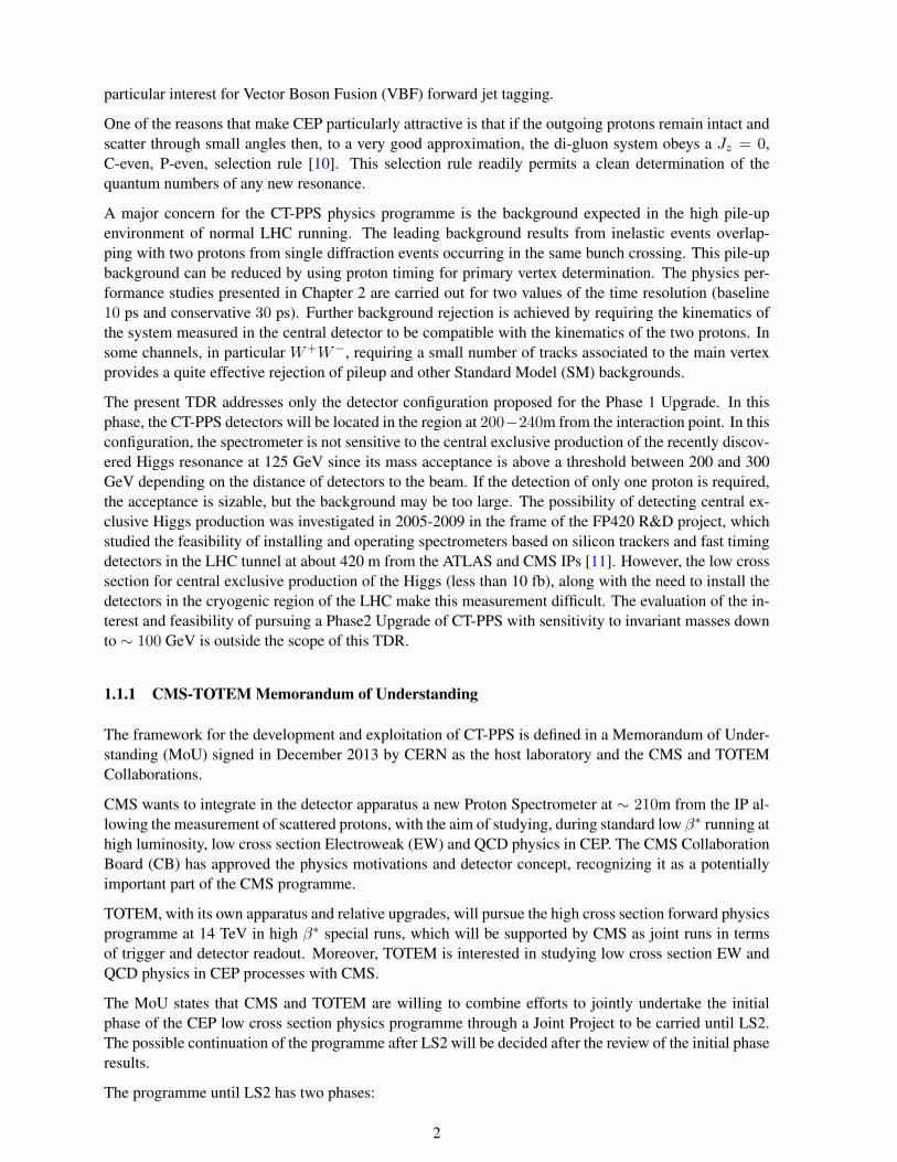
We plan to add precision proton tracking and timing detectors in the very forward region on both sides ofCMS, to study central exclusive production in proton-proton collisions, namely the process pp→ pXp,in which the protons do not dissociate and interact via photon or colour-singlet exchange to producethe system X in the central region. The CMS-TOTEM Precision Proton Spectrometer (CT-PPS) isa magnetic spectrometer that uses the LHC magnets between the Interaction Point (IP) and detectorstations at ∼ 210m from the IP on both sides, to bend protons that have lost a small fraction of theirmomentum out of the beam envelope so their trajectories can be measured. The layout of the beam linein the 210 m region after the first Long Shutdown (LS1) is shown in Figure 1.

The CT-PPS detectors consists of a silicon tracking system to measure the position and direction of theprotons, and a set of timing counters to measure their arrival time. This in turn allows the reconstructionof the mass and momentum as well as the z coordinate of the primary vertex of the centrally producedsystem, irrespective of its decay mode. The detector covers an area of about 4 cm2 on each arm. In totalit uses 144 pixel readout chips and has∼200 timing readout channels. The total cost of the detectors andinfrastructure is below 1 MCHF.

220m 215m 204m àIP5

2 new horizontal cylindrical RPs (1 in LS1)

2 horizontal box-shaped RPs

Figure 1: The layout of the CT-PPS detectors in the 210 m region after LS1. The cylindrical Roman Potsare equipped with timing detectors for PU rejection. The upgraded box-shaped Roman Pots (RPs) areequipped with pixel detectors to measure the displacement of the scattered protons w.r.t. the beam.

Central exclusive production (CEP) provides a unique method to access a variety of physics topics,such as new physics via anomalous production of W and Z boson pairs, high transverse momentum(pT ) jet production, and possibly the production of new resonances. These studies can be carried out inparticularly clean experimental conditions thanks to the absence of proton remnants. The detection of thetwo final state protons, scattered at almost zero-degrees, in very forward near-beam detectors, provides astriking signature. The measurement of the leading protons allows to fully determine the kinematics ofthe central system. Well defined final states in the CMS central detector matching the protons kinematicscan then be selected and precisely reconstructed.

The exclusive two-photon production of pairs of photons, W and Z bosons provides a novel and uniquetesting ground for the electroweak gauge boson sector. The virtualities of the exchanged photons areon average very small, which makes the LHC a quasi-real photon collider with centre-of-mass energyapproaching 1 TeV – a region so far unexplored. The detection of γγ → W+W− events allows tomeasure the quartic gauge coupling WWγγ with high precision. We expect to achieve of the order of103−4 times better sensitivity to anomalous quartic gauge couplings than LEP [1]-[8] and Tevatron [9].

A number of physics studies will be aimed at the understanding of the QCD mechanisms involved inCEP. Exclusive di-jet production with M(jj) up to ∼ 700− 800 GeV allows the study of pure gluon jetsamples with small contamination of quark jets. The detailed characterization of gluon jets in this datasample relative to quark jets may improve the efficiency of gluon vs. quark jets separation, which is of

1

particular interest for Vector Boson Fusion (VBF) forward jet tagging.

One of the reasons that make CEP particularly attractive is that if the outgoing protons remain intact andscatter through small angles then, to a very good approximation, the di-gluon system obeys a Jz = 0,C-even, P-even, selection rule [10]. This selection rule readily permits a clean determination of thequantum numbers of any new resonance.

A major concern for the CT-PPS physics programme is the background expected in the high pile-upenvironment of normal LHC running. The leading background results from inelastic events overlap-ping with two protons from single diffraction events occurring in the same bunch crossing. This pile-upbackground can be reduced by using proton timing for primary vertex determination. The physics per-formance studies presented in Chapter 2 are carried out for two values of the time resolution (baseline10 ps and conservative 30 ps). Further background rejection is achieved by requiring the kinematics ofthe system measured in the central detector to be compatible with the kinematics of the two protons. Insome channels, in particular W+W−, requiring a small number of tracks associated to the main vertexprovides a quite effective rejection of pileup and other Standard Model (SM) backgrounds.

The present TDR addresses only the detector configuration proposed for the Phase 1 Upgrade. In thisphase, the CT-PPS detectors will be located in the region at 200−240m from the interaction point. In thisconfiguration, the spectrometer is not sensitive to the central exclusive production of the recently discov-ered Higgs resonance at 125 GeV since its mass acceptance is above a threshold between 200 and 300GeV depending on the distance of detectors to the beam. If the detection of only one proton is required,the acceptance is sizable, but the background may be too large. The possibility of detecting central ex-clusive Higgs production was investigated in 2005-2009 in the frame of the FP420 R&D project, whichstudied the feasibility of installing and operating spectrometers based on silicon trackers and fast timingdetectors in the LHC tunnel at about 420 m from the ATLAS and CMS IPs [11]. However, the low crosssection for central exclusive production of the Higgs (less than 10 fb), along with the need to install thedetectors in the cryogenic region of the LHC make this measurement difficult. The evaluation of the in-terest and feasibility of pursuing a Phase2 Upgrade of CT-PPS with sensitivity to invariant masses downto ∼ 100 GeV is outside the scope of this TDR.

1.1.1 CMS-TOTEM Memorandum of Understanding

The framework for the development and exploitation of CT-PPS is defined in a Memorandum of Under-standing (MoU) signed in December 2013 by CERN as the host laboratory and the CMS and TOTEMCollaborations.

CMS wants to integrate in the detector apparatus a new Proton Spectrometer at ∼ 210m from the IP al-lowing the measurement of scattered protons, with the aim of studying, during standard low β∗ running athigh luminosity, low cross section Electroweak (EW) and QCD physics in CEP. The CMS CollaborationBoard (CB) has approved the physics motivations and detector concept, recognizing it as a potentiallyimportant part of the CMS programme.

TOTEM, with its own apparatus and relative upgrades, will pursue the high cross section forward physicsprogramme at 14 TeV in high β∗ special runs, which will be supported by CMS as joint runs in termsof trigger and detector readout. Moreover, TOTEM is interested in studying low cross section EW andQCD physics in CEP processes with CMS.

The MoU states that CMS and TOTEM are willing to combine efforts to jointly undertake the initialphase of the CEP low cross section physics programme through a Joint Project to be carried until LS2.The possible continuation of the programme after LS2 will be decided after the review of the initial phaseresults.

The programme until LS2 has two phases:

2

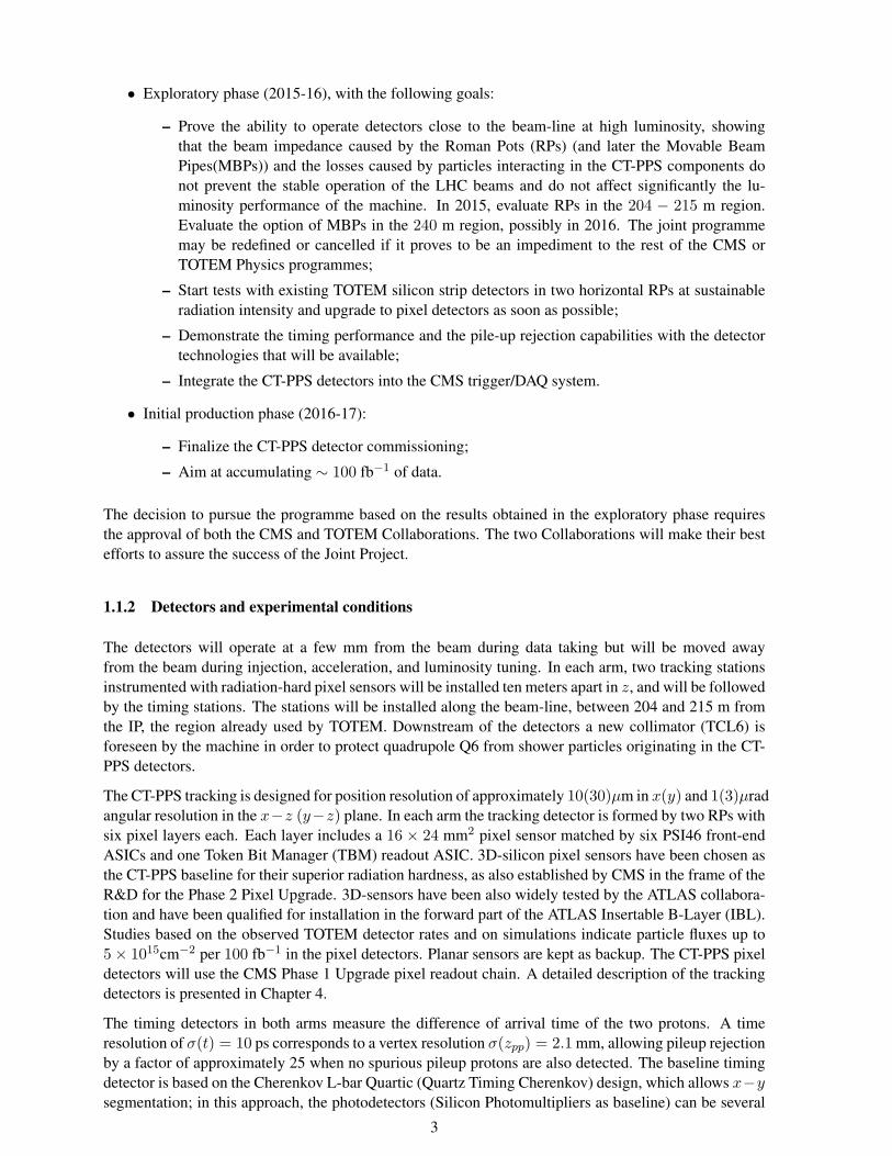
• Exploratory phase (2015-16), with the following goals:

– Prove the ability to operate detectors close to the beam-line at high luminosity, showingthat the beam impedance caused by the Roman Pots (RPs) (and later the Movable BeamPipes(MBPs)) and the losses caused by particles interacting in the CT-PPS components donot prevent the stable operation of the LHC beams and do not affect significantly the lu-minosity performance of the machine. In 2015, evaluate RPs in the 204 − 215 m region.Evaluate the option of MBPs in the 240 m region, possibly in 2016. The joint programmemay be redefined or cancelled if it proves to be an impediment to the rest of the CMS orTOTEM Physics programmes;

– Start tests with existing TOTEM silicon strip detectors in two horizontal RPs at sustainableradiation intensity and upgrade to pixel detectors as soon as possible;

– Demonstrate the timing performance and the pile-up rejection capabilities with the detectortechnologies that will be available;

– Integrate the CT-PPS detectors into the CMS trigger/DAQ system.

• Initial production phase (2016-17):

– Finalize the CT-PPS detector commissioning;

– Aim at accumulating ∼ 100 fb−1 of data.

The decision to pursue the programme based on the results obtained in the exploratory phase requiresthe approval of both the CMS and TOTEM Collaborations. The two Collaborations will make their bestefforts to assure the success of the Joint Project.

1.1.2 Detectors and experimental conditions

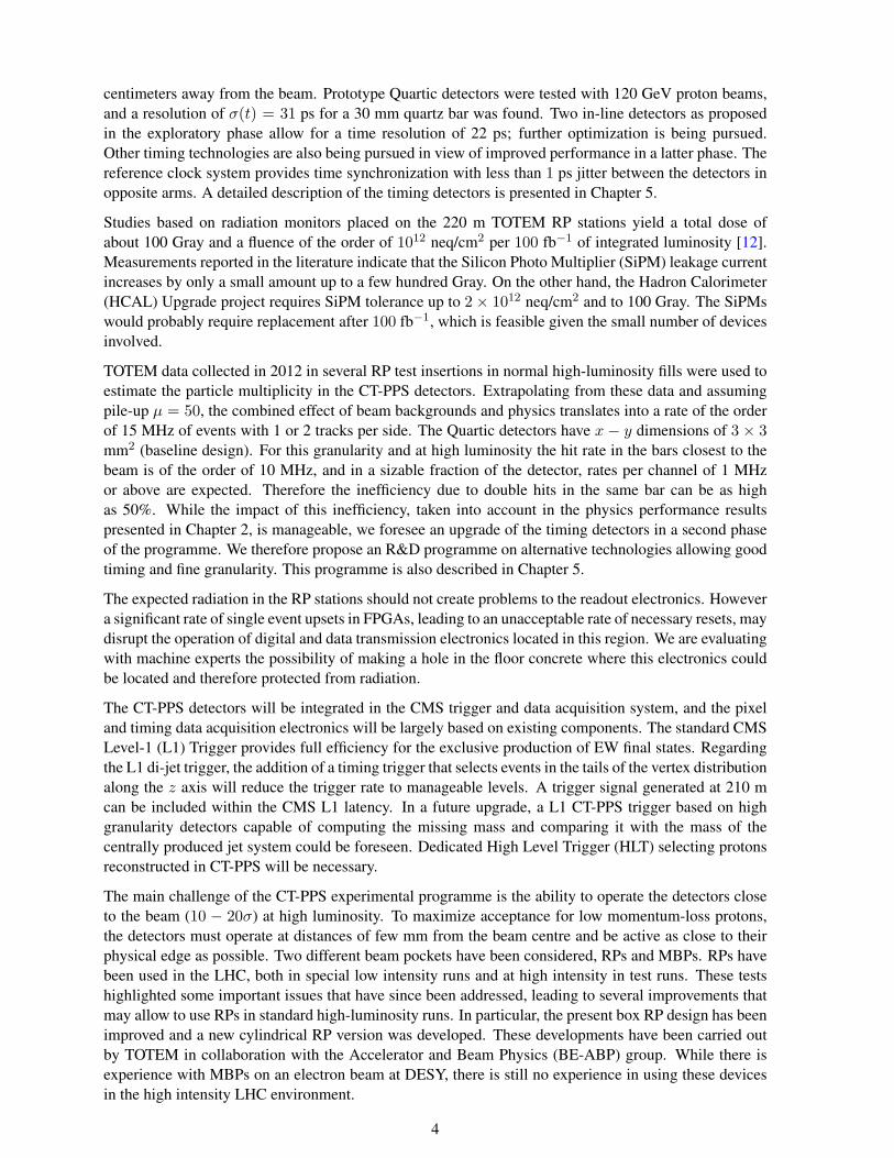
The detectors will operate at a few mm from the beam during data taking but will be moved awayfrom the beam during injection, acceleration, and luminosity tuning. In each arm, two tracking stationsinstrumented with radiation-hard pixel sensors will be installed ten meters apart in z, and will be followedby the timing stations. The stations will be installed along the beam-line, between 204 and 215 m fromthe IP, the region already used by TOTEM. Downstream of the detectors a new collimator (TCL6) isforeseen by the machine in order to protect quadrupole Q6 from shower particles originating in the CT-PPS detectors.

The CT-PPS tracking is designed for position resolution of approximately 10(30)µm in x(y) and 1(3)µradangular resolution in the x−z (y−z) plane. In each arm the tracking detector is formed by two RPs withsix pixel layers each. Each layer includes a 16 × 24 mm2 pixel sensor matched by six PSI46 front-endASICs and one Token Bit Manager (TBM) readout ASIC. 3D-silicon pixel sensors have been chosen asthe CT-PPS baseline for their superior radiation hardness, as also established by CMS in the frame of theR&D for the Phase 2 Pixel Upgrade. 3D-sensors have been also widely tested by the ATLAS collabora-tion and have been qualified for installation in the forward part of the ATLAS Insertable B-Layer (IBL).Studies based on the observed TOTEM detector rates and on simulations indicate particle fluxes up to5× 1015cm−2 per 100 fb−1 in the pixel detectors. Planar sensors are kept as backup. The CT-PPS pixeldetectors will use the CMS Phase 1 Upgrade pixel readout chain. A detailed description of the trackingdetectors is presented in Chapter 4.

The timing detectors in both arms measure the difference of arrival time of the two protons. A timeresolution of σ(t) = 10 ps corresponds to a vertex resolution σ(zpp) = 2.1 mm, allowing pileup rejectionby a factor of approximately 25 when no spurious pileup protons are also detected. The baseline timingdetector is based on the Cherenkov L-bar Quartic (Quartz Timing Cherenkov) design, which allows x−ysegmentation; in this approach, the photodetectors (Silicon Photomultipliers as baseline) can be several

3

centimeters away from the beam. Prototype Quartic detectors were tested with 120 GeV proton beams,and a resolution of σ(t) = 31 ps for a 30 mm quartz bar was found. Two in-line detectors as proposedin the exploratory phase allow for a time resolution of 22 ps; further optimization is being pursued.Other timing technologies are also being pursued in view of improved performance in a latter phase. Thereference clock system provides time synchronization with less than 1 ps jitter between the detectors inopposite arms. A detailed description of the timing detectors is presented in Chapter 5.

Studies based on radiation monitors placed on the 220 m TOTEM RP stations yield a total dose ofabout 100 Gray and a fluence of the order of 1012 neq/cm2 per 100 fb−1 of integrated luminosity [12].Measurements reported in the literature indicate that the Silicon Photo Multiplier (SiPM) leakage currentincreases by only a small amount up to a few hundred Gray. On the other hand, the Hadron Calorimeter(HCAL) Upgrade project requires SiPM tolerance up to 2× 1012 neq/cm2 and to 100 Gray. The SiPMswould probably require replacement after 100 fb−1, which is feasible given the small number of devicesinvolved.

TOTEM data collected in 2012 in several RP test insertions in normal high-luminosity fills were used toestimate the particle multiplicity in the CT-PPS detectors. Extrapolating from these data and assumingpile-up µ = 50, the combined effect of beam backgrounds and physics translates into a rate of the orderof 15 MHz of events with 1 or 2 tracks per side. The Quartic detectors have x − y dimensions of 3 × 3mm2 (baseline design). For this granularity and at high luminosity the hit rate in the bars closest to thebeam is of the order of 10 MHz, and in a sizable fraction of the detector, rates per channel of 1 MHzor above are expected. Therefore the inefficiency due to double hits in the same bar can be as highas 50%. While the impact of this inefficiency, taken into account in the physics performance resultspresented in Chapter 2, is manageable, we foresee an upgrade of the timing detectors in a second phaseof the programme. We therefore propose an R&D programme on alternative technologies allowing goodtiming and fine granularity. This programme is also described in Chapter 5.

The expected radiation in the RP stations should not create problems to the readout electronics. Howevera significant rate of single event upsets in FPGAs, leading to an unacceptable rate of necessary resets, maydisrupt the operation of digital and data transmission electronics located in this region. We are evaluatingwith machine experts the possibility of making a hole in the floor concrete where this electronics couldbe located and therefore protected from radiation.

The CT-PPS detectors will be integrated in the CMS trigger and data acquisition system, and the pixeland timing data acquisition electronics will be largely based on existing components. The standard CMSLevel-1 (L1) Trigger provides full efficiency for the exclusive production of EW final states. Regardingthe L1 di-jet trigger, the addition of a timing trigger that selects events in the tails of the vertex distributionalong the z axis will reduce the trigger rate to manageable levels. A trigger signal generated at 210 mcan be included within the CMS L1 latency. In a future upgrade, a L1 CT-PPS trigger based on highgranularity detectors capable of computing the missing mass and comparing it with the mass of thecentrally produced jet system could be foreseen. Dedicated High Level Trigger (HLT) selecting protonsreconstructed in CT-PPS will be necessary.

The main challenge of the CT-PPS experimental programme is the ability to operate the detectors closeto the beam (10 − 20σ) at high luminosity. To maximize acceptance for low momentum-loss protons,the detectors must operate at distances of few mm from the beam centre and be active as close to theirphysical edge as possible. Two different beam pockets have been considered, RPs and MBPs. RPs havebeen used in the LHC, both in special low intensity runs and at high intensity in test runs. These testshighlighted some important issues that have since been addressed, leading to several improvements thatmay allow to use RPs in standard high-luminosity runs. In particular, the present box RP design has beenimproved and a new cylindrical RP version was developed. These developments have been carried outby TOTEM in collaboration with the Accelerator and Beam Physics (BE-ABP) group. While there isexperience with MBPs on an electron beam at DESY, there is still no experience in using these devicesin the high intensity LHC environment.

4

The additional Radio Frequency (RF) impedance (transversal and longitudinal) introduced by thesedevices is a major concern. As a guideline, the machine (BE-ABP) established that the additionalimpedance should not be larger than about 1% of the total LHC impedance. Nevertheless this thresholdis a safety indication and not a sharp limit. At 1 mm from the beam, the cylindrical RP increases theLHC transverse impedance by 0.5% and the longitudinal by 1.2%. These figures need to be multipliedby four, as four RPs per arm are foreseen. While these values are above the indicative limit mentionedabove, we point out that in the low β∗ beam tests done in 2012 there were no direct evidence of beaminstabilities induced by the RP (see Section 1.3). The MBP design aims at a beam pocket with smallerRF impedance. The present design includes 11-degree tapering structures as in the standard LHC colli-mators. At 1 mm from the beam the transverse impedance increases by 0.05% and the longitudinal by0.5%. The total impedance increase for a single arm (two MBPs per arm) is then about 0.10% trans-versely and 1.0% longitudinally. To these values we should add the impedance of the bellows. On theother hand, the increased material traversed by particles due to the MBP small tapering angle may requireusing beryllium for the thin windows, which raises some mechanical challenges. Additionally, the MBPwould need bellows capable to accommodate a 25 mm transverse stroke.

The test runs performed in 2012 complemented by Fluka simulations indicate that the approach of theRPs to the beam at the distance demanded by physics requires to absorb the showers produced by theRPs in order to protect the downstream quadrupole. The solution envisaged was the addition of the newcollimators (TCL6), which are already installed. A detailed description of the beam pocket structures,including the proposed MBP development programme, is presented in Chapter 3.

We consider that the RP is a more mature solution, in an advanced stage of implementation and suitablefor post-LS1 testing, and therefore we have adopted it for the exploratory phase in 2015. However,considering the uncertainties associated with the operation of these devices at high luminosity, and giventhe potential good performance of MBPs and the benefits for physics of operating the detectors as closeas possible from the beam, we propose that the development of the MBP solution be pursued in parallelwith the goal of installation of a test structure in 2016.

Based on the above considerations, we propose that for the exploratory phase in 2015-16 we use RPsand available silicon strip detectors in conjunction with the central detector. This configuration wouldallow to understand the performance of the new RPs with high intensity beams. One cylindrical RPper arm would also be installed in LS1, allowing the installation Quartic timing detectors in the fall of2015 (during a technical stop) to evaluate the pileup rejection capability of this detector. At the year-endtechnical stop 2015-16 the new pixel detectors would replace the silicon strips. A MBP structure mayalso be installed for tests. The results of the evaluation of MBPs compared to RPs would determinehow to proceed in the following years in view of optimizing the CT-PPS physics potential. Using theexperience acquired in the exploratory phase we expect that significant luminosity could be integrated in2016-17. The aim is to integrate a total luminosity of 100 fb−1 before LS2.

1.2 Physics with the CMS-TOTEM Precision Proton Spectrometers

1.2.1 Introduction to physics with CT-PPS

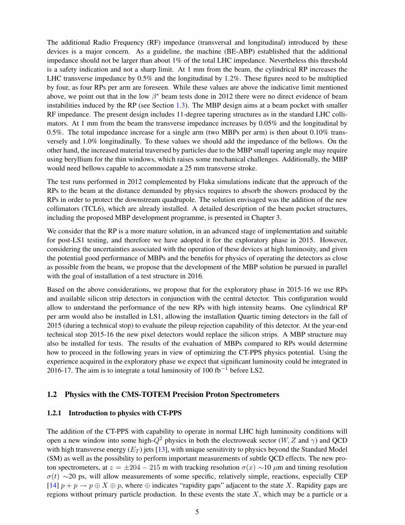
The addition of the CT-PPS with capability to operate in normal LHC high luminosity conditions willopen a new window into some high-Q2 physics in both the electroweak sector (W,Z and γ) and QCDwith high transverse energy (ET ) jets [13], with unique sensitivity to physics beyond the Standard Model(SM) as well as the possibility to perform important measurements of subtle QCD effects. The new pro-ton spectrometers, at z = ±204 − 215 m with tracking resolution σ(x) ∼10 µm and timing resolutionσ(t) ∼20 ps, will allow measurements of some specific, relatively simple, reactions, especially CEP[14] p + p → p ⊕X ⊕ p, where ⊕ indicates “rapidity gaps” adjacent to the state X . Rapidity gaps areregions without primary particle production. In these events the state X , which may be a particle or a

5

more complex, but well-defined state, is measured by the main central detector and its four-momentum isdetermined from the two scattered protons. In this way, CEP events resemble more electron-positron an-nihilation events than normal LHC events, in which the initial state of the interacting partons or particlesis not well known since hadrons are composite objects.

In CEP reactions, the mass of state X , M(X), can be reconstructed from the fractional momentum loss,ξ1 and ξ2, of the scattered protons by M(X) = M(pp) ∼

√ξ1ξ2s. The M(X) reach at the LHC will

be significantly larger than that of previous colliders (ISR, SppS and Tevatron) because of the larger√s.

For the first time we will be able to study CEP at the electroweak scale.

In standard LHC high-luminosity optics, the scattered protons can be observed mainly thanks to theirmomentum loss, via their horizontal deviation from the beam centre at the position of the CT-PPS. Thistranslates into a lower limit in ξ (and hence in M(X)), below which there is no acceptance for thesimultaneous detection of the two protons in a CEP reaction. The value of this threshold depends on thedistance from the IP and on how close to the beam the proton detectors can be moved. At

√s = 13 TeV

and in normal high-luminosity conditions, with the CT-PPS detectors at 15σ from the beam, values ofM(X) & 300 GeV will be accessible. CEP reactions at such high masses have cross sections that aretypically about 1 fb and thus can only be studied in the normal high-luminosity running, with µ & 30inelastic interactions per bunch crossing. This is complementary to the special high β∗ runs [15], whereany CEP M(X) can be studied as long as the cross section is of order 1 pb or higher.

CEP is a t-channel exchange process, and the absolute value of the four-momentum-transfer squared, |t|,follows an approximately exponentially decreasing distribution. The carrier of this t-channel exchangemust be neutral in flavour, colour, and electric charge. In the SM, the allowed t-channel exchangesare only photons γ, gluons g (if their colour is neutralised), and Z-bosons. We first discuss two-photoncollisions, then gluon-gluon fusion with an additional gluon exchange to neutralise the colour, and finallyphotoproduction.

1.2.2 Two-photon collisions

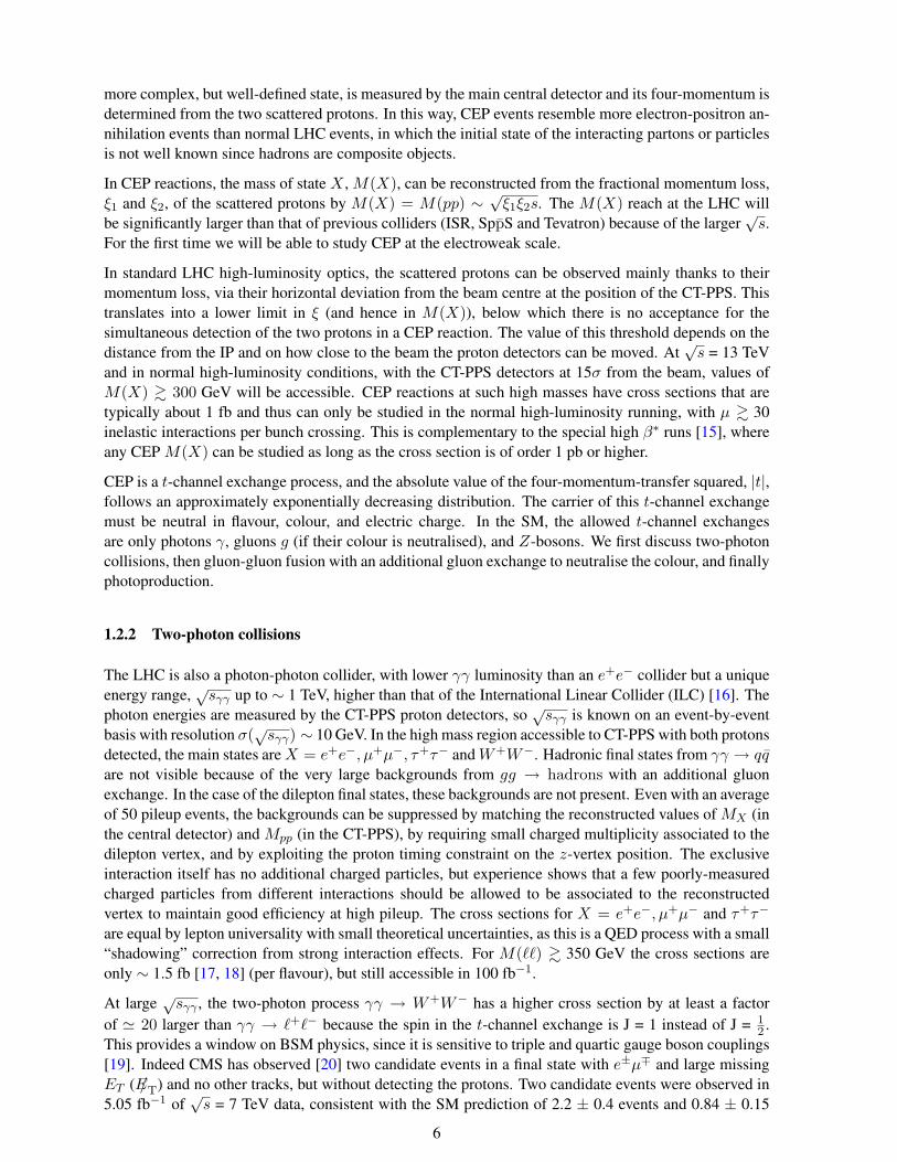
The LHC is also a photon-photon collider, with lower γγ luminosity than an e+e− collider but a uniqueenergy range, √sγγ up to ∼ 1 TeV, higher than that of the International Linear Collider (ILC) [16]. Thephoton energies are measured by the CT-PPS proton detectors, so √sγγ is known on an event-by-eventbasis with resolution σ(√sγγ) ∼ 10 GeV. In the high mass region accessible to CT-PPS with both protonsdetected, the main states areX = e+e−, µ+µ−, τ+τ− andW+W−. Hadronic final states from γγ → qqare not visible because of the very large backgrounds from gg → hadrons with an additional gluonexchange. In the case of the dilepton final states, these backgrounds are not present. Even with an averageof 50 pileup events, the backgrounds can be suppressed by matching the reconstructed values of MX (inthe central detector) and Mpp (in the CT-PPS), by requiring small charged multiplicity associated to thedilepton vertex, and by exploiting the proton timing constraint on the z-vertex position. The exclusiveinteraction itself has no additional charged particles, but experience shows that a few poorly-measuredcharged particles from different interactions should be allowed to be associated to the reconstructedvertex to maintain good efficiency at high pileup. The cross sections for X = e+e−, µ+µ− and τ+τ−

are equal by lepton universality with small theoretical uncertainties, as this is a QED process with a small“shadowing” correction from strong interaction effects. For M(``) & 350 GeV the cross sections areonly ∼ 1.5 fb [17, 18] (per flavour), but still accessible in 100 fb−1.

At large √sγγ , the two-photon process γγ → W+W− has a higher cross section by at least a factorof ' 20 larger than γγ → `+`− because the spin in the t-channel exchange is J = 1 instead of J = 1

2 .This provides a window on BSM physics, since it is sensitive to triple and quartic gauge boson couplings[19]. Indeed CMS has observed [20] two candidate events in a final state with e±µ∓ and large missingET (E/T) and no other tracks, but without detecting the protons. Two candidate events were observed in5.05 fb−1 of

√s = 7 TeV data, consistent with the SM prediction of 2.2 ± 0.4 events and 0.84 ± 0.15

6

background. This resulted in limits on the Anomalous Quartic Gauge Couplings (AQGC) parameters ofthe order of 1.5(5) ×10−4 GeV−2 for aW

0(c)/Λ2, assuming a dipole form factor with the energy cutoff

scale at Λcutoff = 500 GeV, which are about 20 times more stringent than the best Tevatron limits, andtwo orders of magnitude better than the best LEP limits.

With an integrated luminosity of 100 fb−1, the CT-PPS is expected to improve the limits by at least twoorders of magnitude, or perhaps observe a deviation from the SM prediction. The SM cross section ishigher at

√s = 13 TeV by a factor∼ 2.5 [21] and the matching of the reconstructed proton vertex coordi-

nate, zpp, with that from the leptons, z``, should allow also the study of the e+e−E/T and µ+µ−E/T finalstates, thus increasing the signal yields. The E/T requirement effectively excludes backgrounds fromγγ → `+`−, which tend to have pT (``) . a few GeV and, for a given M(X), the γγ → `+`− crosssections are smaller than the γγ → W+W− ones by more than an order of magnitude. Measuringthe protons provides kinematic constraints and reduces significantly the backgrounds. The semileptoniccase, X = W+W− → `±νjj, is also accessible by requiring “track gaps”, i.e. no tracks associated tothe vertex with large momentum transverse to any jet axis. The proton measurements give M(W+W−),and one can even check that M(`±ν) = M(W ). These modes give a factor of six more statistics. Kine-matic distributions may also be used to increase the sensitivity to AQGC [19]. Results on the CT-PPSsensitivity to W+W− CEP obtained from detailed simulations are presented in Chapter 2.

Exclusive γγ → ZZ and γγ → γγ provide unique measurements of quartic gauge couplings withonly neutral particles [22]. They measure dimension-eight operators; one example, from R.S. Gupta[23], is the exchange of a Kaluza-Klein graviton if there are large extra dimensions. The γγ → ZZ orγγ processes are only allowed through loops in the SM resulting in ab-range cross sections within theCT-PPS mass acceptance, so even a few events in 100 fb−1 may offer an opportunity for a new physicsdiscovery. BothX = γγ and ZZ processes can be accessible with cross sections of the order of 1−10 fbwithin the CT-PPS mass range in some allowed scenarios. In the ZZ case, one may study the case whereone of the Z decay hadronically, using kinematic constraints and track-gap requirements to reduce thebackgrounds. In the γγ case, the primary vertex is reconstructed from the protons: allowing one of thephotons to be a converted one, a match between the vertexes (from photons and protons) is possibleand a better background rejection can be achieved. In addition, the two photons have similar transversemomentum (pT) values, and are approximately back-to-back in azimuthal angle. These selection criteriashould allow sensitivity for the γγ channel even in high pile-up conditions [24].

1.2.3 Tests of Quantum Chromodynamics

Normally, in gluon-guon interactions the colour exchange results in multi-hadron production. Howeverin multi-jet (two-, three-, or four-jet) exclusive production a third gluon of opposite colour is exchangedand a colour string does not form. This may result in one or more rapidity gaps unless another parton-parton interaction occurs. The probability that this does not happen and the gap is preserved is calledthe “rapidity gap survival probability” S2. The overall suppression relative to inclusive jj production isabout 10−5 for M(X) ∼ 350 GeV. In low-Q2 interactions, including elastic scattering and diffractiveexcitation, this colour-singlet gluon pair is the leading order description of the Pomeron PI .

CEP of high-ET jets will shed light on a number of crucial aspects of the proton structure and the stronginteraction. On the one hand, the two-gluon proton vertex measures the (skewed) unintegrated gluonparton distribution function of the proton, in a region never explored before. On the other hand, theexperimental study of the rapidity gap survival probability opens up a new window on the study of softmultiple parton interactions. Finally, to a very good approximation, the final state obeys a Jz = 0, C-even, P-even, selection rule [25]. Here Jz is the projection of the total angular momentum along theproton beam axis. This selection rule readily permits a clean determination of the quantum numbers ofany new resonance. In other words, if a new state were to be produced in CEP, not only could its massbe determined precisely from the scattered protons momenta, independent of the decay mode, but also

7

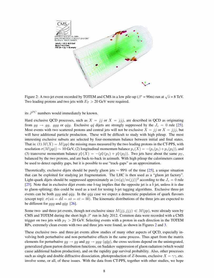
Figure 2: A two-jet event recorded by TOTEM and CMS in a low pile-up (β∗ = 90m) run at√s = 8 TeV.

Two leading protons and two jets with ET > 20 GeV were required.

its JPC numbers would immediately be known.

Hard exclusive QCD processes, such as X = jj or X = jjj, are described in QCD as originatingfrom gg → gg, ggg or qqg. Exclusive qq dijets are strongly suppressed by the Jz = 0 rule [25].Most events with two scattered protons and central jets will not be exclusive X = jj or X = jjj, butwill have additional particle production. These will be difficult to study with high pileup. The mostinteresting exclusive subsets are selected by four-momentum balance between initial and final states.That is: (1)M(X) = M(pp) the missing mass measured by the two leading protons in the CT-PPS, withresolution σ(M(pp)) ∼ 10 GeV, (2) longitudinal momentum balance pz(X) = −(pz(p1)+pz(p2)), and(3) transverse momentum balance ~pT (X) = −( ~pT (p1) + ~pT (p2)). Two jets have about the same pT ,balanced by the two protons, and are back-to-back in azimuth. With high pileup the calorimeters cannotbe used to detect rapidity gaps, but it is possible to use “track-gaps” as an approximation.

Theoretically, exclusive dijets should be purely gluon jets ∼ 99% of the time [25], a unique situationthat can be exploited for studying jet fragmentation. The LHC is then used as a “gluon jet factory”.Light-quark dijets should be suppressed approximately as (m(q)/m(jj))2 according to the Jz = 0 rule[25]. Note that in exclusive dijet events one b-tag implies that the opposite jet is a b jet, unless it is dueto gluon-splitting; this could be used as a tool for testing b-jet tagging algorithms. Exclusive three-jetevents can be both ggg and qqg. In the qqg case we expect a democratic population of quark flavours(except top): σ(uu = dd = ss = cc = bb). The kinematic distributions of the three jets are expected tobe different for ggg and qqg [26].

Some two- and three-jet events, though not exclusive since M(jj, jjj) M(pp), were already seen byCMS and TOTEM during the short high β∗ run in July 2012. Common data were recorded with a CMStrigger on two jets with pT > 20 GeV. Selecting events with a proton in each direction in the TOTEMRPs, extremely clean events with two and three jets were found, as shown in Figures 2 and 3.

These exclusive two- and three-jet events allow studies of many other aspects of QCD, especially in-volving both perturbative and non-perturbative effects in the same process. Thus apart from the matrixelements for perturbative gg → gg and gg → ggg (qqg), the cross sections depend on the unintegrated,generalized gluon parton distribution functions, on Sudakov suppression of gluon radiation (which wouldcause additional hadron production), and on the rapidity gap survival probability. Also, other processessuch as single and double diffractive dissociation, photoproduction of Z-bosons, exclusive X = γγ, etc.involve some, or all, of these issues. With the data from CT-PPS, together with other studies, we hope

8

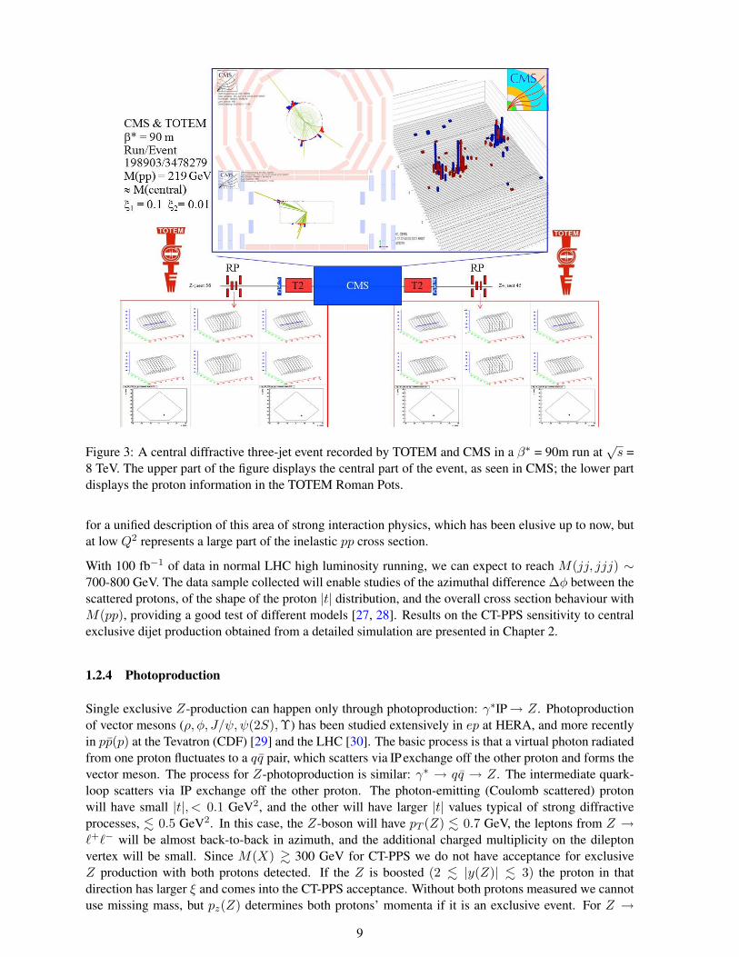
Figure 3: A central diffractive three-jet event recorded by TOTEM and CMS in a β∗ = 90m run at√s =

8 TeV. The upper part of the figure displays the central part of the event, as seen in CMS; the lower partdisplays the proton information in the TOTEM Roman Pots.

for a unified description of this area of strong interaction physics, which has been elusive up to now, butat low Q2 represents a large part of the inelastic pp cross section.

With 100 fb−1 of data in normal LHC high luminosity running, we can expect to reach M(jj, jjj) ∼700-800 GeV. The data sample collected will enable studies of the azimuthal difference ∆φ between thescattered protons, of the shape of the proton |t| distribution, and the overall cross section behaviour withM(pp), providing a good test of different models [27, 28]. Results on the CT-PPS sensitivity to centralexclusive dijet production obtained from a detailed simulation are presented in Chapter 2.

1.2.4 Photoproduction

Single exclusive Z-production can happen only through photoproduction: γ∗ PI → Z. Photoproductionof vector mesons (ρ, φ, J/ψ, ψ(2S),Υ) has been studied extensively in ep at HERA, and more recentlyin pp(p) at the Tevatron (CDF) [29] and the LHC [30]. The basic process is that a virtual photon radiatedfrom one proton fluctuates to a qq pair, which scatters via PI exchange off the other proton and forms thevector meson. The process for Z-photoproduction is similar: γ∗ → qq → Z. The intermediate quark-loop scatters via PI exchange off the other proton. The photon-emitting (Coulomb scattered) protonwill have small |t|, < 0.1 GeV2, and the other will have larger |t| values typical of strong diffractiveprocesses, . 0.5 GeV2. In this case, the Z-boson will have pT (Z) . 0.7 GeV, the leptons from Z →`+`− will be almost back-to-back in azimuth, and the additional charged multiplicity on the dileptonvertex will be small. Since M(X) & 300 GeV for CT-PPS we do not have acceptance for exclusiveZ production with both protons detected. If the Z is boosted (2 . |y(Z)| . 3) the proton in thatdirection has larger ξ and comes into the CT-PPS acceptance. Without both protons measured we cannotuse missing mass, but pz(Z) determines both protons’ momenta if it is an exclusive event. For Z →

9

µ+µ− events, as well as with the two-photon events γγ → µ+µ−, this provides a valuable calibration(or check) of the momentum scale of the proton spectrometers. One can also use the low additionalcharged multiplicity requirement on the vertex and the kinematics to observe Z photoproduction withoutdetecting the protons, but in that case either one or both protons could dissociate into massive clustersand the cross section is affected in a way that is not very well known.

It should be noted that high mass central exclusive dijet production, pp→ p⊕ jj ⊕ p, can also occur viaphotoproduction in a C = −1 state [31]. The cross section of this process is expected to be significantlylower than the corresponding one from gg fusion.

To conclude, the addition of small but very precise tracking and timing detectors far along the beams,CT-PPS, opens up a whole new field in both electroweak physics, including BSM sensitivity, and QCD,for a very modest cost.

1.3 Strategy and running scenarios

1.3.1 Exploratory phase

LHC Start-Up ScenarioThe LHC strategy for the start-up after LS1 is outlined in [32]. After a short commissioning period ata bunch spacing of 50 ns, operation at 25 ns will be attempted. Reaching the desired peak luminosity of(1÷2)×1034 cm−2s−1 with 50 ns bunch spacing would imply bunches of 1.6×1011 protons leading to apileup level of µ ∼ 80÷120, more than the experiments can tolerate. Operation with 50 ns bunch spacingand luminosity levelling would be a fall-back scenario for the first year in case of major difficulties with25 ns bunch spacing. This option would bring considerable complications for the CT-PPS programme.Firstly, the enormous pileup would be difficult to resolve even with 10 ps time resolution. Secondly, theluminosity levelling is implemented by changing β∗ in steps during a fill, modifying each time the beamoptics and the beam width at the RP positions. Whether the RP positions need to be adapted in everyβ∗ step remains to be studied. However, as laid out in the following sections, RP operation for physicsproduction at high luminosity is not expected for the first year. When the timing detectors are installedin the RPs, operation at 25 ns bunch spacing will very likely be standard.

Roman Pot insertion commissioningThe first important goal after LS1 is to gain experience with RP insertions and their interplay with thecollimation system. After the impedance heating and the resulting vacuum deteriorations observed inhigh-luminosity insertion tests in late 2012, the RP system underwent a series of improvements [15,33], and the new cylindrical RPs were designed accordingly [34]. Verifying the effectiveness of thesemeasures is the first milestone to be met.

The RP insertion tests will exploit the following diagnostic instrumentation:

• Beam Loss Monitors (BLMs): The BLMs measure the dose rate due to showers produced bythe interaction of beam halo or IP5 collision debris with RPs or collimators. Their beam dumpthresholds are defined in view of protecting downstream magnets from quenching.

• Vacuum gauges: A pressure rise near the RPs can be an indication of impedance heating.

• Early detector instrumentation in the new cylindrical RPs: In the very first stage after LS1, whiletiming detectors are not yet available for installation, the new RPs will be equipped with tempo-rary diagnostic detectors. In addition to temperature measurements with PT100 sensors, to assessimpedance heating, particle rate information will be available either from scintillators (segmentedor monolithic) or from a pair of TOTEM’s edgeless silicon strip detectors. Together with theBLMs, these detectors will enable the mapping of the halo and debris profile.

10

The insertion tests will proceed in a sequence of increasingly challenging beam conditions.

The first step will be the beam-based RP alignment subsequent to the alignment of the collimators. At lowβ∗ all the RP units (horizontal and vertical pots) and the new cylindrical RPs have to be aligned. This partof the LHC commissioning procedure will be performed with a beam intensity allowing the “restrictedsetup beam flag” to be set, i.e. not more than 1.4× 1011 protons per beam at 6.5 TeV. According to pre-LS1 RP alignment experience, no insertion difficulties are expected, but first knowledge about the rateprofile can be obtained. This alignment, followed by loss-map validations of the collimator hierarchy forthe nominal RP position settings is a prerequisite for all later RP insertions. The nominal horizontal RPpositions depend on the details of the collimation scheme, which has not yet been finalised. They areexpected to lie between 12 and 15 sigma from the beam centre, i.e. about 1 sigma in the shadow of thetertiary collimators, TCTs.

The next RP insertions will be carried out in end-of-fill studies, i.e. with a certain time delay afterdeclaration of stable beams, to be agreed in the LPC, in order to minimise the impact of possible beamdumps on the LHC data production. The goal of these insertion tests is to find an optimal set of positionsnot only of the RPs but also of the collimators TCL4, TCL5 and TCL6, offering sufficient protectionfor the magnets downstream of RPs without cutting too much into the proton acceptance of the RPs.Conservatively, for the first such insertion the beams will be separated by 5 ÷ 6σ in IP5 to reduce theluminosity (cf. Table 1) and thus the debris background, facilitating the RP approach. This separationcan then be successively reduced, leading to increasingly harsh background conditions. Once a viableset of RP and TCL positions has been found for zero beam separation, the system will be ready for thefirst physics runs.

Timing Detector CommissioningAfter establishing the optimal set of TCL and RP positions, and after installation of timing detectorsin the new RPs, first physics runs for timing studies will be performed. To avoid entering immediatelyinto the most difficult pileup domain with µ ∼ 40, the commissioning of the timing detector systemwill be done in end-of-fill studies with separated beams like in the RP insertion commissioning phase.Table 1 shows the luminosity reach and the pileup level as a function of the beam separation for a typicalstandard running scenario with 25 ns bunch spacing. For separations above about 3.8σ, the pileup leveldrops below 1. At µ = 1, an end-of-fill run of 1 hour would not only allow tests of the timing systemat a comfortable occupancy but also the collection of about 1 pb−1 of data. Finally, the beam separationcould be gradually reduced to arrive at the full luminosity and the full pileup of regular LHC fills.

1.3.2 Data production phase

After the commissioning steps described in the previous sections, the RP system will be fully validatedfor continuous operation in all regular LHC fills. At that stage, the RP insertion movements will beimplemented in operational sequences to be executed by the LHC operator immediately after declarationof stable beams.

While details of the beam conditions and bunching schemes are not yet fully defined and will dependon the experience gathered in the post-LS1 recommissioning phase, the common aim of the LHC ex-periments and the machine experts is to operate with 25 ns rather than 50 ns bunch spacing in order tokeep the pileup manageable. Possible options are shown in Table 2. In all cases a peak luminosity of theorder 1034 cm−2 s−1 and a pileup between 20 and 50 are envisaged. In such conditions, 100 fb−1 can becollected in about 100 full days.

11

d [σ] [µm] µ L [cm−2 s−1] L/day

0 0 39.1 1.30× 1034 1.1 fb−1

1 11.7 30.4 1.01× 1034 0.85 fb−1

2 23.4 14.4 4.79× 1033 0.41 fb−1

3 35.1 4.12 1.37× 1033 0.12 fb−1

3.8 44.8 1.00 3.34× 1032 28 pb−1

4 46.8 0.715 2.38× 1032 20 pb−1

5 58.6 0.075 2.51× 1031 2.1 pb−1

6 70.3 0.005 1.61× 1030 0.14 pb−1

Table 1: Inelastic pileup µ and luminosity L as a function of the beam separation d in the IP. Commonparameters: β∗ = 0.5 m, E = 6.5 TeV, 2520 colliding bunches (i.e. with a spacing of 25 ns) of 1.15 ×1011 protons, full crossing angle = 310µrad, εn = 1.9µm rad, bunch length σz = 10.12 cm, inelasticcross-section = 85 mb.

Table 2: Expected beam parameters and peak performance for 25 ns bunch spacing at 6.5 TeV(from [32]).

12

References

[1] G. Belanger et al., “Bosonic quartic couplings at LEP-2”, Eur. Phys. J. C 13 (2000) 283.

[2] ALEPH Collaboration, “Constraints on anomalous QGCs in e+e− interactions from 183 GeV to209 GeV”, Phys. Lett. B 602 (2004) 31.

[3] OPAL Collaboration, “Constraints on anomalous quartic gauge boson couplings from ννγγ andqqγγ events at LEP-2”, Phys. Rev. D 70 (2004) 032005.

[4] OPAL Collaboration, “A study of W+W−γ events at LEP”, Phys. Lett. B 580 (2004) 17.

[5] OPAL Collaboration, Measurement of the W+W−γ cross-section and first direct limits on anoma-lous electroweak quartic gauge couplings, Phys. Lett. B 471 (1999) 293.

[6] L3 Collaboration, “The e+e− → Zγγ → qq reaction at LEP and constraints on anomalous quarticgauge boson couplings”, Phys. Lett. B 540 (2002) 43.

[7] L3 Collaboration, “Study of the W+W−γ process and limits on anomalous quartic gauge bosoncouplings at LEP”, Phys. Lett. B 527 (2002) 29.

[8] DELPHI Collaboration, “Measurement of the e+e− → W+W−γ cross-section and limits onanomalous quartic gauge couplings with DELPHI”, Eur. Phys. J. C 31 (2003) 139.

[9] D0 Collaboration, “Search for anomalous quartic WWγγ couplings in dielectron and missing en-ergy final states in ppbar collisions at

√s = 1.96 TeV”, arXiv:1305.1258 (2013).

[10] See e.g. V.A.Khoze,A.D.Martin and M.G.Ryskin, “Double diffractive processes in high res-olution missing mass experiments at the Tevatron”, Eur.Phys.J.C19:477-483,2001; Erratum-ibid.C20:599,2001 [hep-ph/0011393].

[11] M.G. Albrow et al., The FP420 R&D Project, “Higgs and New Physics with forward protons atLHC”, JINST 4 (2009) T10001.

[12] F. Ravotti, “Update on TOTEM Roman Pots, T1 and T2 Radiation Levels (Summary of first threeyear LHC running period)”, CERN EDMS 1353932. https://edms.cern.ch/document/1353932

[13] The CMS and TOTEM diffractive and forward physics working group, “Prospects for Diffractiveand Forward Physics at the LHC”, CERN/LHCC 2006-039/G-124 (2006).

[14] See e.g. M.G. Albrow, T.D. Coughlin, and J.R. Forshaw, Prog. Part. Nucl. Phys. 65 (2010) 149.

[15] TOTEM Collaboration, “TOTEM Upgrade Proposal”, CERN-LHCC-2013-009; LHCC-P-007 and“Timing Measurements in the Vertical Roman Pots of the TOTEM Experiment”, CERN-LHCC-2014-020 (TOTEM-TDR-002).

[16] K. Piotrzkowski, “Tagging Two-Photon Production at the LHC”, Phys. Rev. D 63, 071502(R).

[17] J.A.M. Vermaseren, Nucl. Phys. B229 (1983) 347.

[18] S.P. Baranov, O. Duenger, H. Shooshtari, J.A.M. Vermaseren, “LPAIR: a generator for lepton pairproduction”, in the proceedings of Physics at HERA, October 29-30, Hamburg, Germany (1991).

[19] See e.g. T. Pierzchala and K. Piotrzkowski, Nucl. Phys. Proc. Suppl. 179-180 (2008) 257.

[20] S.Chatrchyan et al. (CMS Collaboration), JHEP 1307 (2013) 116.

13

https://edms.cern.ch/document/1353932

https://edms.cern.ch/document/1353932

[21] M. Luszczak and A. Szczurek, “Subleading processes in production of W+W− pairs in proton-proton collisions”, arXiv:1405.0018, (2013).

[22] D.d’Enterria and G.G.Silveira, “Observing light-by-light scattering at the Large Hadron Collider”,Phys.Rev.Lett. 111 (2013) 080405

[23] R.S. Gupta, Phys. Rev. D 85 (2012) 014006.

[24] S. Fichet et al., “Probing new physics in diphoton production with proton tagging at the LargeHadron Collider”, arXiv:1312.5153.

[25] V.A. Khoze, A.D. Martin, and M.G. Ryskin, Eur. Phys. J. C 48 (2001) 477 and erratum ibid. C 20(2001) 599.

[26] V.A. Khoze, M.G. Ryskin and W.J. Stirling, Eur. Phys. J. C 19 (2006) 477.

[27] L.A. Harland-Lang, V.A. Khoze, M.G. Ryskin and W.J. Stirling, “Central exclusive productionwithin the Durham model: a review”, IPPP-14-42, DCPT-14-84 (2014), arXiv:1405.0018.

[28] V.A. Petrov and R.A. Ryutin, J.Phys. G 35 (2008) 065004; R.A. Ryutin, Eur. Phys. J. C 73 (2013)2443.

[29] T.Aaltonen et al., PRL 102, 242001 (2009).

[30] R. Aaij et al, J. Phys. G: Nucl. Part. Phys. 41 (2014) 055002.

[31] V.A. Khoze, private communication.

[32] G. Arduini, “ Post LS1 Operation”, Proceedings of the MPP Workshop, March 2013.https://indico.cern.ch/event/227895

[33] J. Baechler et al., “TOTEM Consolidation Project”, LHC-XRP-EC-0010, EDMS 1314925.

[34] M. Deile et al., “TOTEM Upgrade Project”, LHC-XRP-EC-0011, EDMS 1361537.

14

https://indico.cern.ch/event/227895

2 Detector and Physics Performance

A discussion of the performance of the CT-PPS tracking and timing detectors is presented. Specifically,the feasibility is discussed of measuring central exclusive production of dijets through gluon-gluon inter-action, and central exclusive production ofW boson pairs in two-photon interactions, in the experimentalconditions foreseen for Run 2.

A brief description of the beam optics is provided in Section 2.1, details of the simulated samples aregiven in Section 2.2, detector acceptance and resolution are presented in Sections 2.3 and 2.4. Theestimate of the machine-induced background is described in Section 2.6, and the RP alignment in Sec-tion 2.7. Finally, the sensitivity of CT-PPS to the two reference physics processes mentioned above isdiscussed in Section 2.8.

2.1 Beam optics

The proposed forward tracking and timing detector stations are to be installed in the regions located atapproximately z=204 m and z=215 m from the IP, in both beam directions downstream of the centraldetector. Protons that have lost energy in the primary interaction emerge laterally after passing throughthe bending magnets. At z=204-215 m one can detect protons that have lost a few percent (' 3− 20%)of the initial beam energy.

The trajectory of protons produced with transverse position (x∗, y∗) and angle (Θ∗x,Θ

∗y) at the IP location

(the ’∗’ superscript indicates the IP location at IP5) is described by the equation

~d = T · ~d∗ , (2.1)

where the vector ~d = (x,Θx, y,Θy,∆p/p) and T is the transport matrix; p and ∆p denote the nominalbeam momentum and the proton longitudinal momentum loss, respectively. The transport matrix isdefined by the optical functions as:

T =

vx Lx m13 m14 Dx

dvxds

dLxds m23 m24

dDxds

m31 m32 vy Ly Dy

m41 m42dvy

dsdLy

dsdDy

ds

0 0 0 0 1

(2.2)

where the magnification vx,y =√βx,y/β∗ cos ∆φx,y, and the effective lengthLx,y =

√βx,yβ∗ sin∆φx,y

are functions of the betatron amplitude βx,y and the relative phase advance up to the RP location∆φx,y =

∫ RP

IPds

β(s)x,y. Together with the dispersion Dx,y (where nominally Dy = 0), they are of particu-

lar importance for the reconstruction of the proton kinematics. In these studies, a proton beam energy of6.5 TeV with the LHC standard optics files (v6.5) is used.

Figure 4 shows the values of the effective lengths in x and y (Lx and Ly) and the corresponding disper-sions (Dx and Dy) as a function of ξ = ∆p/p (momentum loss of the surviving proton) at the detectorlocation at z=204 m. These values, together with the beam widths and divergences, determine accep-tance and resolution for the proton kinematic variables t (four-momentum transfer squared) and ξ. Inthe present study, no uncertainty in the optical function is assumed. Once data-taking starts, the opticalfunctions (and their resolutions) will be determined from the beam optics actually used for any given fill,according to the method discussed in Ref. [1].

The configuration of the LHC beam-line around the CMS IP is shown in Figure 5 for z > 0.

15

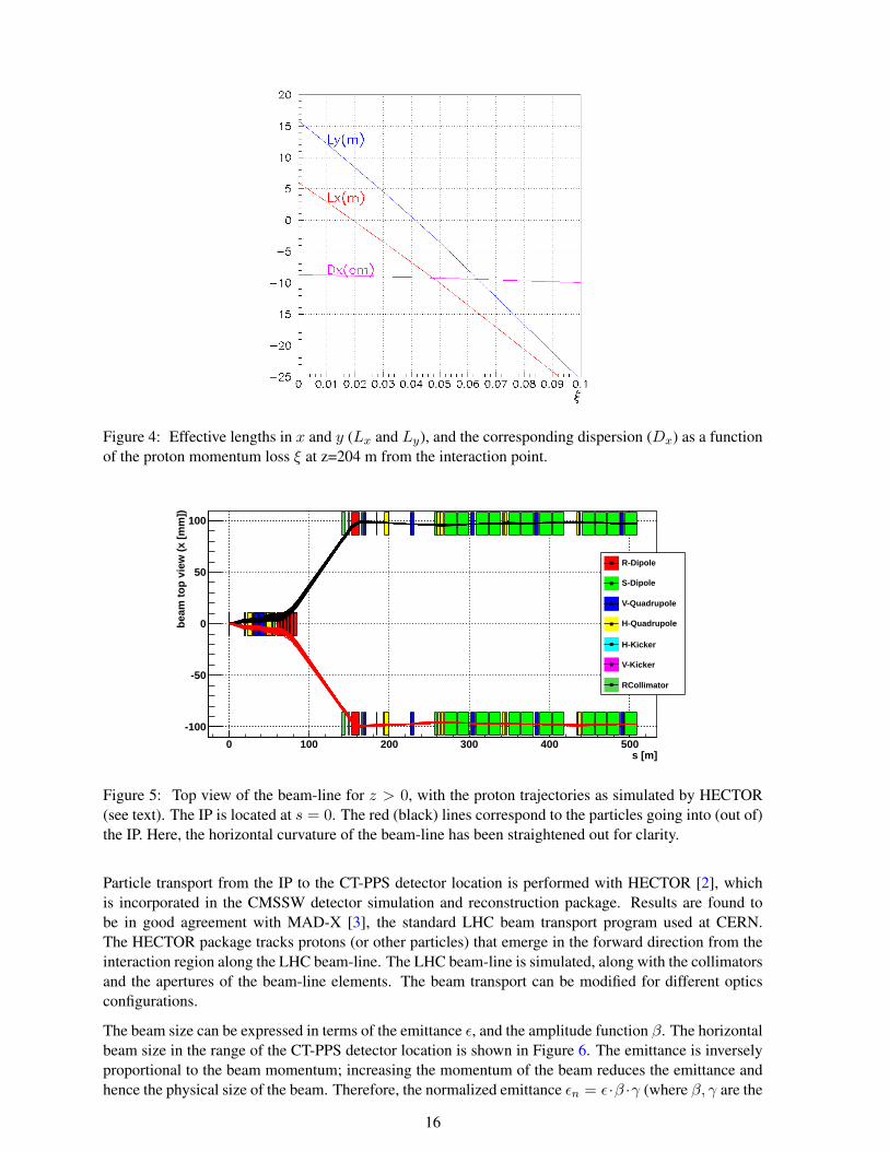
Figure 4: Effective lengths in x and y (Lx and Ly), and the corresponding dispersion (Dx) as a functionof the proton momentum loss ξ at z=204 m from the interaction point.

s [m]0 100 200 300 400 500

bea

m t

op

vie

w (

x [m

m])

-100

-50

0

50

100

R-Dipole

S-Dipole

V-Quadrupole

H-Quadrupole

H-Kicker

V-Kicker

RCollimator

Figure 5: Top view of the beam-line for z > 0, with the proton trajectories as simulated by HECTOR(see text). The IP is located at s = 0. The red (black) lines correspond to the particles going into (out of)the IP. Here, the horizontal curvature of the beam-line has been straightened out for clarity.

Particle transport from the IP to the CT-PPS detector location is performed with HECTOR [2], whichis incorporated in the CMSSW detector simulation and reconstruction package. Results are found tobe in good agreement with MAD-X [3], the standard LHC beam transport program used at CERN.The HECTOR package tracks protons (or other particles) that emerge in the forward direction from theinteraction region along the LHC beam-line. The LHC beam-line is simulated, along with the collimatorsand the apertures of the beam-line elements. The beam transport can be modified for different opticsconfigurations.

The beam size can be expressed in terms of the emittance ε, and the amplitude function β. The horizontalbeam size in the range of the CT-PPS detector location is shown in Figure 6. The emittance is inverselyproportional to the beam momentum; increasing the momentum of the beam reduces the emittance andhence the physical size of the beam. Therefore, the normalized emittance εn = ε·β ·γ (where β, γ are the

16

relativistic functions) is often used instead. The amplitude function at the IP is taken to be β∗ = 0.6 m,the normalized emittance εn ' 3.75 · 10−6 m (emittance ε ' 5.4 · 10−10 m), and the crossing angle142.5µrad in the horizontal plane. A vertex resolution of σ∗x,y = 15µm and an angular beam divergenceof σ∗θ = 30µrad at the IP are assumed [4].

Figure 6: Horizontal distance to the beam center in the region 200 < z < 225 m corresponding to thelocation of tracking and timing detector stations with the 15σx and 20σx Roman Pot approaches. Theparameters used for the optics are described in the text.

2.2 Simulated samples

The performance of the CT-PPS is quantified in terms of the ability to measure two reference pro-cesses: central exclusive production of dijets, pp → pJJp, and central exclusive production of W pairs,pp → pWWp. The exclusive dijet sample is simulated with the ExHuME (v1.3.2) [5] generator in-terfaced with PYTHIA (v6.426) [6]; the γγ → WW signal is generated using FPMC (v1.0) [7], withHERWIG 6.5 [8] used to simulate the decay of the W+W− pair. Events are generated for

√s = 13 TeV

in the region 0 < |t| < 4 GeV2 and 0.01 < ξ < 0.2. For the backgrounds, Single Diffractive (SD)and Double Pomeron Exchange (DPE) exclusive events are generated using POMWIG (v2.0) interfacedwith HERWIG (v6.521) [8], multijet QCD events are simulated using PYTHIA (v8.175) [9], inclusive WWevents with PYTHIA (v6.426), while the exclusive γγ → ττ events are generated with FPMC.

The presence of multiple interactions per bunch crossing (pileup) is incorporated by simulating additionalinteractions with an average pileup multiplicity of µ = 50 matching that expected during Run 2. PYTHIA

(v6.4 for the exclusive WW analysis, and v8.175 for that of the exclusive dijets) is used to generateminimum bias samples, including diffractive events. These events are mixed with the signal events tosimulate the data-taking conditions expected during Run 2.

The generated events are processed through the GEANT4 (v9.4p03) [10] simulation of the CMS centraldetector and the standard reconstruction chain. Protons are tracked through the beam-line all the way tothe position of the tracking and timing detectors. The simulation includes the beam energy dispersion,the beam crossing angle, smearing due to the beam divergence, vertex smearing, and detector resolutioneffects. In the CT-PPS, tracking and timing detectors are not fully simulated. The baseline timingdetector (QUARTIC) has dimensions of 20 × 18 mm2 (in x, y), with a segmentation of 3 × 3 mm2;time resolution values of 10 ps (baseline) and 30 ps (conservative) are considered. For the trackingdetectors, the resolution is simulated by a gaussian smearing of 10 µm on the proton position propagated

17

at z=204 m and z=215 m.

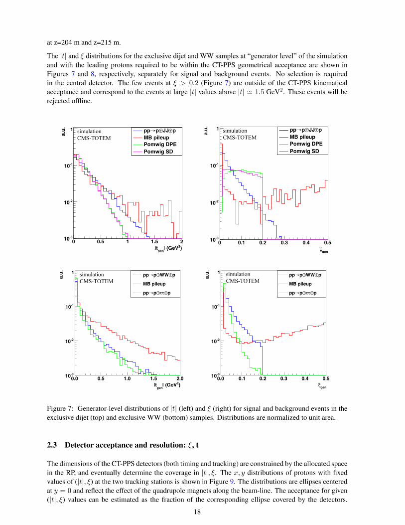
The |t| and ξ distributions for the exclusive dijet and WW samples at “generator level” of the simulationand with the leading protons required to be within the CT-PPS geometrical acceptance are shown inFigures 7 and 8, respectively, separately for signal and background events. No selection is requiredin the central detector. The few events at ξ > 0.2 (Figure 7) are outside of the CT-PPS kinematicalacceptance and correspond to the events at large |t| values above |t| ' 1.5 GeV2. These events will berejected offline.

)2| (GeVgen|t0 0.5 1 1.5 2

a.u.

-310

-210

-110

1 p⊕JJ⊕p→ppMB pileupPomwig DPEPomwig SD

simulation CMS-TOTEM

genξ0 0.1 0.2 0.3 0.4 0.5

a.u.

-310

-210

-110



)2| (GeVgen|t0.0 0.5 1.0 1.5 2.0

a.u.

-310

-210

-110

1 p⊕WW⊕p→pp

MB pileup

p⊕ττ⊕p→pp


genξ0.0 0.1 0.2 0.3 0.4 0.5

a.u.

-310

-210

-110

1 p⊕WW⊕p→pp

MB pileup

p⊕ττ⊕p→pp


Figure 7: Generator-level distributions of |t| (left) and ξ (right) for signal and background events in theexclusive dijet (top) and exclusive WW (bottom) samples. Distributions are normalized to unit area.

2.3 Detector acceptance and resolution: ξ, t

The dimensions of the CT-PPS detectors (both timing and tracking) are constrained by the allocated spacein the RP, and eventually determine the coverage in |t|, ξ. The x, y distributions of protons with fixedvalues of (|t|, ξ) at the two tracking stations is shown in Figure 9. The distributions are ellipses centeredat y = 0 and reflect the effect of the quadrupole magnets along the beam-line. The acceptance for given(|t|, ξ) values can be estimated as the fraction of the corresponding ellipse covered by the detectors.

18

)2| (GeVgen|t0 0.5 1 1.5 2

a.u.

-310

-210

-110



genξ0 0.1 0.2 0.3 0.4 0.5

a.u.

-310

-210

-110



)2| (GeVgen|t0.0 0.5 1.0 1.5 2.0

a.u.

-310

-210

-110

1 p⊕WW⊕p→pp

MB pileup

p⊕ττ⊕p→pp


genξ0.0 0.1 0.2 0.3 0.4 0.5

a.u.

-310

-210

-110

1 p⊕WW⊕p→pp

MB pileup

p⊕ττ⊕p→pp


Figure 8: Distributions of generated |t| (left) and ξ (right) for signal and background events in theexclusive dijet (top) and exclusive WW (bottom) samples. Distributions are normalized to unit area.Coincidence of hits in the tracking stations at z=204 m and z=215 m (on one side of the IP) is required.Tracking detectors are located at a distance of 15 σ from the beam center. Smearing effects due to vertexposition, beam energy dispersion and crossing angle are accounted for.

Figure 9 is obtained with a “particle gun”, generating protons at fixed (|t|, ξ) values, in conjunction withHECTOR.

Concerning the detector distance from the beam center, the following approach is used: the RP window isplaced at 15 (20) σ from the beam center and the distance of the sensors from the RP window is assumedto be 0.3 mm. The additional dead region due to the inefficiency of the sensor edge is not accounted for;it is estimated to be between 0.1 mm and 0.2 mm, which corresponds to 1− 2σ of the beam dimensions.In Figure 9, the rectangle drawn by a dashed (solid) black line illustrates the boundaries of a detectorwith an area (in x, y) of 20 × 18 mm2 located at 15σ (20σ)+0.3 mm from the beam center, whereas thebeam envelopes are schematically drawn by ellipses centered at zero.

As mentioned above, no detailed simulation of the silicon detectors has been included, as their finaldesign and characteristics are still being finalized. A detector resolution of 10 µm is accounted for bysmearing the proton simulated position at the detector location. The other key parameters in the present

19

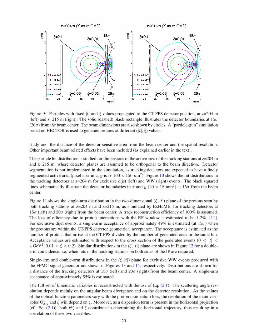
Figure 9: Particles with fixed |t| and ξ values propagated to the CT-PPS detector position, at z=204 m(left) and z=215 m (right). The solid (dashed) black rectangle illustrates the detector boundaries at 15σ(20σ) from the beam center. The beam dimensions are also shown by circles. A “particle-gun” simulationbased on HECTOR is used to generate protons at different (|t|, ξ) values.

study are: the distance of the detector sensitive area from the beam center and the spatial resolution.Other important beam related effects have been included (as explained earlier in the text).

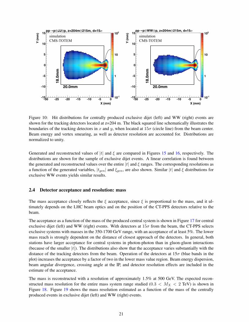
The particle hit distribution is studied for dimensions of the active area of the tracking stations at z=204 mand z=215 m, where detector planes are assumed to be orthogonal to the beam direction. Detectorsegmentation is not implemented in the simulation, as tracking detectors are expected to have a finelysegmented active area (pixel size in x, y is ≈ 100 × 150 µm2). Figure 10 shows the hit distributions inthe tracking detectors at z=204 m for exclusive dijet (left) and WW (right) events. The black squaredlines schematically illustrate the detector boundaries in x and y (20 × 18 mm2) at 15σ from the beamcenter.

Figure 11 shows the single-arm distribution in the two-dimensional (ξ, |t|) plane of the protons seen byboth tracking stations at z=204 m and z=215 m, as simulated by ExHuME, for tracking detectors at15σ (left) and 20σ (right) from the beam center. A track reconstruction efficiency of 100% is assumed.The loss of efficiency due to proton interactions with the RP window is estimated to be 1-2% [11].For exclusive dijet events, a single-arm acceptance of approximately 49% is estimated (at 15σ) whenthe protons are within the CT-PPS detector geometrical acceptance. The acceptance is estimated as thenumber of protons that arrive at the CT-PPS divided by the number of generated ones in the same bin.Acceptance values are estimated with respect to the cross section of the generated events (0 < |t| <4 GeV2, 0.01 < ξ < 0.2). Similar distributions in the (ξ, |t|) plane are shown in Figure 12 for a double-arm coincidence, i.e. when hits in the tracking stations on both sides of the IP are required.

Single-arm and double-arm distributions in the (ξ, |t|) plane for exclusive WW events produced withthe FPMC signal generator are shown in Figures 13 and 14, respectively. Distributions are shown fora distance of the tracking detectors at 15σ (left) and 20σ (right) from the beam center. A single-armacceptance of approximately 55% is estimated.

The full set of kinematic variables is reconstructed with the use of Eq. (2.1). The scattering angle res-olution depends mainly on the angular beam divergence and on the detector resolution. As the valuesof the optical function parameters vary with the proton momentum loss, the resolution of the main vari-ables Θ∗

x,y and ξ will depend on ξ. Moreover, as a dispersion term is present in the horizontal projection(cf. Eq. (2.1)), both Θ∗

x and ξ contribute in determining the horizontal trajectory, thus resulting in acorrelation of these two variables.

20

X (mm)-30 -25 -20 -15 -10 -5 0

Y (m

m)

-15

-10

-5

0

5

10

15

-110

1

10

210σ215m, d=15⊕p, z=204m⊕JJ⊕p→pp

20.0mm

18.0

mm


X (mm)-30 -25 -20 -15 -10 -5 0

Y (m

m)

-15

-10

-5

0

5

10

15

-110

1

10

210σ215m, d=15⊕p, z=204m⊕WW⊕p→pp

20.0mm

18.0

mm


Figure 10: Hit distributions for centrally produced exclusive dijet (left) and WW (right) events areshown for the tracking detectors located at z=204 m. The black squared line schematically illustrates theboundaries of the tracking detectors in x and y, when located at 15σ (circle line) from the beam center.Beam energy and vertex smearing, as well as detector resolution are accounted for. Distributions arenormalized to unity.

Generated and reconstructed values of |t| and ξ are compared in Figures 15 and 16, respectively. Thedistributions are shown for the sample of exclusive dijet events. A linear correlation is found betweenthe generated and reconstructed values over the entire |t| and ξ ranges. The corresponding resolutions asa function of the generated variables, |tgen| and ξgen, are also shown. Similar |t| and ξ distributions forexclusive WW events yields similar results.

2.4 Detector acceptance and resolution: mass

The mass acceptance closely reflects the ξ acceptance, since ξ is proportional to the mass, and it ul-timately depends on the LHC beam optics and on the position of the CT-PPS detectors relative to thebeam.

The acceptance as a function of the mass of the produced central system is shown in Figure 17 for centralexclusive dijet (left) and WW (right) events. With detectors at 15σ from the beam, the CT-PPS selectsexclusive systems with masses in the 350-1700 GeV range, with an acceptance of at least 5%. The lowermass reach is strongly dependent on the distance of closest approach of the detectors. In general, bothstations have larger acceptance for central systems in photon-photon than in gluon-gluon interactions(because of the smaller |t|). The distributions also show that the acceptance varies substantially with thedistance of the tracking detectors from the beam. Operation of the detectors at 15σ (blue bands in theplot) increases the acceptance by a factor of two in the lower mass value region. Beam energy dispersion,beam angular divergence, crossing angle at the IP, and detector resolution effects are included in theestimate of the acceptance.

The mass is reconstructed with a resolution of approximately 1.5% at 500 GeV. The expected recon-structed mass resolution for the entire mass system range studied (0.3 < MX < 2 TeV) is shown inFigure 18. Figure 19 shows the mass resolution estimated as a function of the mass of the centrallyproduced events in exclusive dijet (left) and WW (right) events.

21

ξ

0.05 0.10 0.15 0.20

)2|t|

(GeV

0.0

0.5

1.0

1.5

2.0

2.5

3.0

3.5

4.0

0

10

20

30

40

50

60

70

80

90

100σ215m, d=15⊕p, z=204m⊕JJ⊕p→pp


ξ

0.05 0.10 0.15 0.20)2

|t| (G

eV0.0

0.5

1.0

1.5

2.0

2.5

3.0

3.5

4.0

0

10

20

30

40

50

60

70

80

90

100σ215m, d=20⊕p, z=204m⊕JJ⊕p→pp


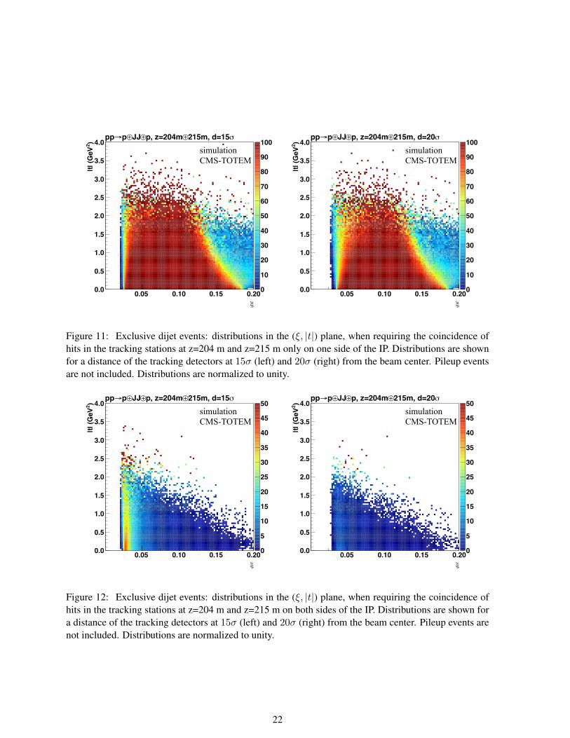
Figure 11: Exclusive dijet events: distributions in the (ξ, |t|) plane, when requiring the coincidence ofhits in the tracking stations at z=204 m and z=215 m only on one side of the IP. Distributions are shownfor a distance of the tracking detectors at 15σ (left) and 20σ (right) from the beam center. Pileup eventsare not included. Distributions are normalized to unity.

ξ

0.05 0.10 0.15 0.20

)2|t|

(GeV

0.0

0.5

1.0

1.5

2.0

2.5

3.0

3.5

4.0

0

5

10

15

20

25

30

35

40

45

50σ215m, d=15⊕p, z=204m⊕JJ⊕p→pp


ξ

0.05 0.10 0.15 0.20

)2|t|

(GeV

0.0

0.5

1.0

1.5

2.0

2.5

3.0

3.5

4.0

0

5

10

15

20

25

30

35

40

45

50σ215m, d=20⊕p, z=204m⊕JJ⊕p→pp


Figure 12: Exclusive dijet events: distributions in the (ξ, |t|) plane, when requiring the coincidence ofhits in the tracking stations at z=204 m and z=215 m on both sides of the IP. Distributions are shown fora distance of the tracking detectors at 15σ (left) and 20σ (right) from the beam center. Pileup events arenot included. Distributions are normalized to unity.

22

ξ

0.05 0.10 0.15 0.20

)2|t|

(GeV

0.0

0.5

1.0

1.5

2.0

2.5

3.0

3.5

4.0

0

10

20

30

40

50

60

70

80

90

100σ215m, d=15⊕p, z=204m⊕WW⊕p→pp


ξ

0.05 0.10 0.15 0.20)2

|t| (G

eV0.0

0.5

1.0

1.5

2.0

2.5

3.0

3.5

4.0

0

10

20

30

40

50

60

70

80

90

100σ215m, d=20⊕p, z=204m⊕WW⊕p→pp


Figure 13: Exclusive WW events: distributions in the (ξ, |t|) plane, when requiring the coincidence ofhits in the tracking stations at z=204 m and z=215 m only on one side of the IP. Distributions are shownfor a distance of the tracking detectors at 15σ (left) and 20σ (right) from the beam center. Pileup eventsare not included. Distributions are normalized to unity.

ξ

0.05 0.10 0.15 0.20

)2|t|

(GeV

0.0

0.5

1.0

1.5

2.0

2.5

3.0

3.5

4.0

0

5

10

15

20

25

30

35

40

45

50σ215m, d=15⊕p, z=204m⊕WW⊕p→pp


ξ

0.05 0.10 0.15 0.20

)2|t|

(GeV

0.0

0.5

1.0

1.5

2.0

2.5

3.0

3.5

4.0

0

5

10

15

20

25

30

35

40

45

50σ215m, d=20⊕p, z=204m⊕WW⊕p→pp


Figure 14: Exclusive WW events: distributions in the (ξ, |t|) plane, at z=204 m and z=215 m on bothsides of the IP. Distributions are shown for a distance of the tracking detectors at 15σ (left) and 20σ(right) from the beam center. Pileup events are not included. Distributions are normalized to unity.

23

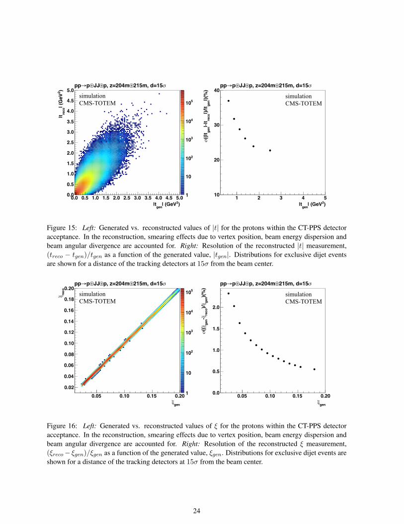
)2| (GeVgen|t0.0 0.5 1.0 1.5 2.0 2.5 3.0 3.5 4.0 4.5 5.0

)2| (

GeV

reco

|t

0.0

0.5

1.0

1.5

2.0

2.5

3.0

3.5

4.0

4.5

5.0

1

10

210

310

410

510

σ215m, d=15⊕p, z=204m⊕JJ⊕p→pp


)2| (GeVgen|t1 2 3 4 5

|)(%

)ge

n|)/

|tre

co|-|

tge

n((|

tσ

10

20

30

40σ215m, d=15⊕p, z=204m⊕JJ⊕p→pp


Figure 15: Left: Generated vs. reconstructed values of |t| for the protons within the CT-PPS detectoracceptance. In the reconstruction, smearing effects due to vertex position, beam energy dispersion andbeam angular divergence are accounted for. Right: Resolution of the reconstructed |t| measurement,(treco − tgen)/tgen as a function of the generated value, |tgen|. Distributions for exclusive dijet eventsare shown for a distance of the tracking detectors at 15σ from the beam center.

genξ0.05 0.10 0.15 0.20

reco

ξ

0.02

0.04

0.06

0.08

0.10

0.12

0.14

0.16

0.18

0.20

1

10

210

310

410

510σ215m, d=15⊕p, z=204m⊕JJ⊕p→pp


genξ0.05 0.10 0.15 0.20

)(%)

gen

ξ)/re

coξ-

gen

ξ((σ

0.0

0.5

1.0

1.5

2.0

σ215m, d=15⊕p, z=204m⊕JJ⊕p→pp σ215m, d=15⊕p, z=204m⊕JJ⊕p→pp


Figure 16: Left: Generated vs. reconstructed values of ξ for the protons within the CT-PPS detectoracceptance. In the reconstruction, smearing effects due to vertex position, beam energy dispersion andbeam angular divergence are accounted for. Right: Resolution of the reconstructed ξ measurement,(ξreco− ξgen)/ξgen as a function of the generated value, ξgen. Distributions for exclusive dijet events areshown for a distance of the tracking detectors at 15σ from the beam center.

24

(GeV)XM500 1000 1500 2000

acce

ptan

ce(%

)

0

10

20

30

40

50

60

70

80

90

100215m⊕p, z=204m⊕JJ⊕p→pp

σd=15

σd=20simulation CMS-TOTEM

(GeV)XM500 1000 1500 2000

acce

ptan

ce(%

)

10

20

30

40

50

60

70

80

90

100215m⊕p, z=204m⊕WW⊕p→pp

σd=15

σd=20simulation CMS-TOTEM

Figure 17: Mass acceptance as a function of centrally produced mass for exclusive dijet events producedin gluon fusion (left, computed with ExHuME), and exclusive WW events produced in photon-photonprocesses (right, computed with FPMC). In the simulation, a coincidence of the tracking detectors placedat z=204 m and z=215 m is required. The estimated acceptance is shown as a solid blue (red) line whenthe tracking detectors are located at a distance of 15 (20) σ from the beam center. Shaded bands indicatethe statistical uncertainties.

2.5 Timing detectors

The occupancy and performance of the time-of-flight detectors are studied for different detector geome-tries. Here again, an average of 50 pileup interactions mixed with the primary interaction is assumed.Smearing effects due to vertex position, beam energy dispersion, beam angular divergence, and crossingangle are simulated.

Segmentation of the timing detector active area is considered for both the baseline option of the QUAR-TIC detectors, and for the study-option of solid state finely-segmented “diamond-like” detectors (dis-cussed in Sections 5.5 and 5.6). The QUARTIC timing detector geometry is physically limited by thetransversal dimensions of the detector bars and by the size of the available photodetectors, but also by theoutgoing proton direction/angle, as each particle must be contained within the same detector bar in orderto maximize the signal yield and minimize the cross-talk between neighboring bars. We estimate that thelatter is not a limiting factor as, at the CT-PPS location, the deflection in x per mm travelled in z is small,and less than ∆x(per mm) ' 0.10 µm. On the other hand, the “diamond-like” detector segmentationoffers a flexible geometry by allowing the optimization of the detector occupancy depending on the dis-tance from the beam center, thus reducing the occupancy rates closer to the beam. In the simulation, eachL-shaped QUARTIC bar has the same (x, y) transversal section of 3× 3 mm2; the “diamond-like” cellshave a y-dimension of 5 mm, with a variable width (in x) varying from 0.3 mm (close to the beam) upto 4.6 mm (away from the beam). Multiple hits in the same cell “blind” the detector functionality, andtherefore –when this happens– the time-of-flight information cannot be used for rejecting pileup events.Such instances are thus contributing as a source of inefficiency to the data analysis. Figure 20 showsthe resulting occupancies for the two geometries, when pileup and beam-related backgrounds (as dis-cussed in detail in Section 2.6) are considered. It is clear that the diamond-like configuration is superior.However, even with average pileup of 50, the baseline configuration is still able to function.

Occupancy distributions (at the z-location of the timing detectors) are compared in Figure 21 for differentaverage pileup multiplicities of µ = 25 and µ = 50. For this additional study, samples analogous to thosediscussed in Section 2.2 and with an average number of pileup interactions µ = 25 are produced. In view

25

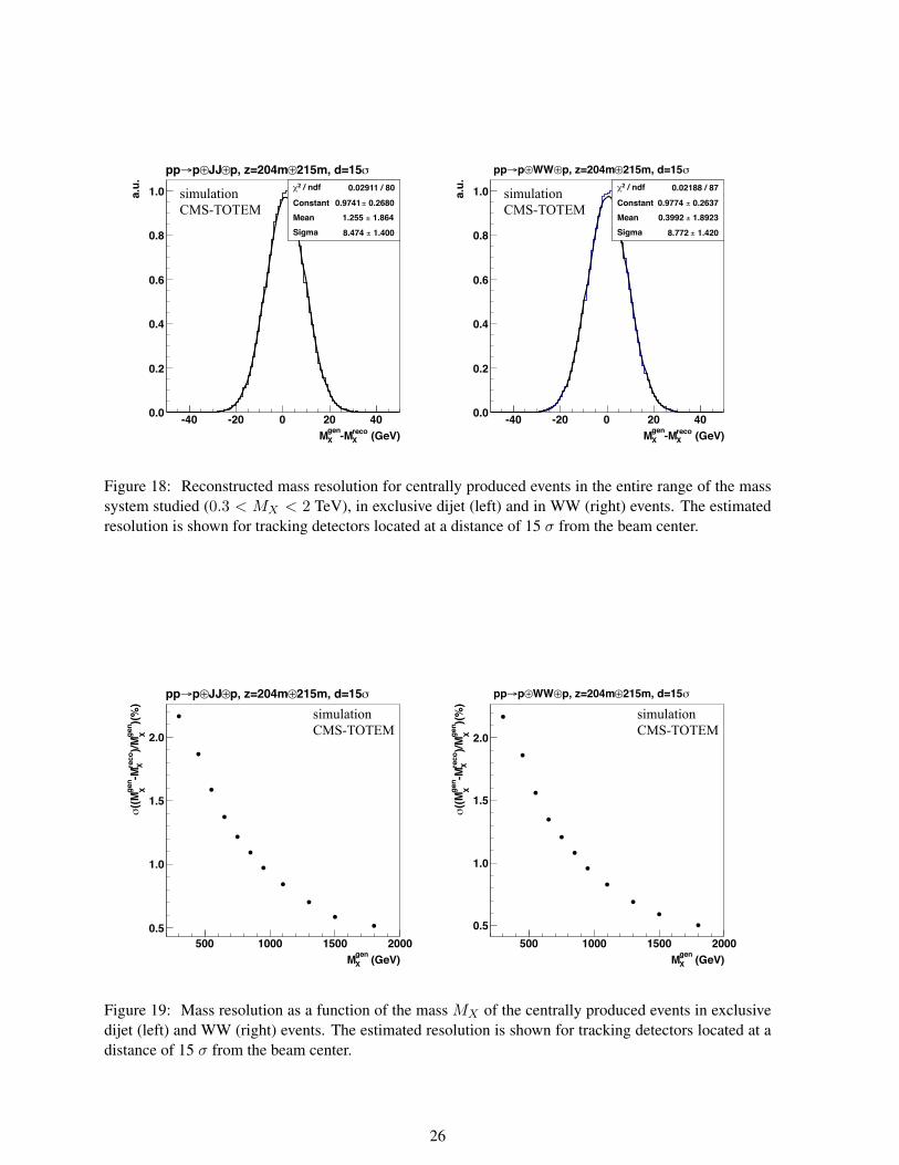
/ ndf 2χ 0.02911 / 80

Constant 0.2680± 0.9741 Mean 1.864± 1.255 Sigma 1.400± 8.474

(GeV)recoX-Mgen

XM-40 -20 0 20 40

a.u.

0.0

0.2

0.4

0.6

0.8

1.0

σ215m, d=15⊕p, z=204m⊕JJ⊕p→pp / ndf 2χ 0.02911 / 80


σ215m, d=15⊕p, z=204m⊕JJ⊕p→pp


/ ndf 2χ 0.02188 / 87


(GeV)recoX-Mgen

XM-40 -20 0 20 40

a.u.

0.0

0.2

0.4

0.6

0.8

1.0

σ215m, d=15⊕p, z=204m⊕WW⊕p→pp / ndf 2χ 0.02188 / 87


σ215m, d=15⊕p, z=204m⊕WW⊕p→pp


Figure 18: Reconstructed mass resolution for centrally produced events in the entire range of the masssystem studied (0.3 < MX < 2 TeV), in exclusive dijet (left) and in WW (right) events. The estimatedresolution is shown for tracking detectors located at a distance of 15 σ from the beam center.

(GeV)genXM

500 1000 1500 2000

)(%)

gen

X)/M

reco

X-M

gen

X((M

σ

0.5

1.0

1.5

2.0

σ215m, d=15⊕p, z=204m⊕JJ⊕p→pp σ215m, d=15⊕p, z=204m⊕JJ⊕p→ppsimulation CMS-TOTEM

(GeV)genXM

500 1000 1500 2000

)(%)

gen

X)/M

reco

X-M

gen

X((M

σ

0.5

1.0

1.5

2.0

σ215m, d=15⊕p, z=204m⊕WW⊕p→pp σ215m, d=15⊕p, z=204m⊕WW⊕p→pp


Figure 19: Mass resolution as a function of the mass MX of the centrally produced events in exclusivedijet (left) and WW (right) events. The estimated resolution is shown for tracking detectors located at adistance of 15 σ from the beam center.

26

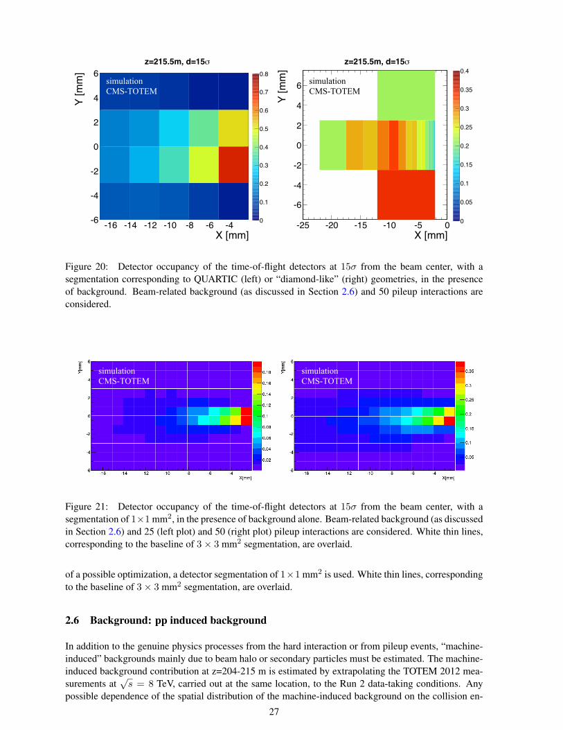
X [mm]-16 -14 -12 -10 -8 -6 -4

Y [m

m]

-6

-4

-2

0

2

4

6

0

0.1

0.2

0.3

0.4

0.5

0.6

0.7

0.8

σz=215.5m, d=15


X [mm]-25 -20 -15 -10 -5 0

Y [m

m]

-6

-4

-2

0

2

4

6

0

0.05

0.1

0.15

0.2

0.25

0.3

0.35

0.4σz=215.5m, d=15


Figure 20: Detector occupancy of the time-of-flight detectors at 15σ from the beam center, with asegmentation corresponding to QUARTIC (left) or “diamond-like” (right) geometries, in the presenceof background. Beam-related background (as discussed in Section 2.6) and 50 pileup interactions areconsidered.



Figure 21: Detector occupancy of the time-of-flight detectors at 15σ from the beam center, with asegmentation of 1×1 mm2, in the presence of background alone. Beam-related background (as discussedin Section 2.6) and 25 (left plot) and 50 (right plot) pileup interactions are considered. White thin lines,corresponding to the baseline of 3× 3 mm2 segmentation, are overlaid.

of a possible optimization, a detector segmentation of 1×1 mm2 is used. White thin lines, correspondingto the baseline of 3× 3 mm2 segmentation, are overlaid.

2.6 Background: pp induced background

In addition to the genuine physics processes from the hard interaction or from pileup events, “machine-induced” backgrounds mainly due to beam halo or secondary particles must be estimated. The machine-induced background contribution at z=204-215 m is estimated by extrapolating the TOTEM 2012 mea-surements at

√s = 8 TeV, carried out at the same location, to the Run 2 data-taking conditions. Any

possible dependence of the spatial distribution of the machine-induced background on the collision en-

27

ergy and the number of bunches in LHC is not taken into account. Different approaches have been usedto understand how to extract the background component from the data and how to extrapolate it to higherpile-up conditions. The detailed procedure is described in [12]. It can be summarized as in the following:the background probability per bunch-crossing is estimated from a zero-bias data sample. The zero-biassample includes all events, from both background and physics processes. In order to subtract the contri-bution from physics processes, the multiplicity of the leading protons reconstructed in the horizontal potsis estimated with a dedicated sample of simulated events (without pileup). By comparing the multiplicityof the primary tracks with the average cluster multiplicity per detector plane from the data (zero-bias datasample) it is then possible to subtract this contribution, and to extract the probability distribution of thebackground per bunch-crossing. These results are then used to extract the scale factors to be applied to asimulation with µ = 50, and extrapolate the tracking multiplicity due to machine-induced backgroundsexpected for Run 2 conditions. The resulting forward (z > 0) and backward (z < 0) RP cluster mul-tiplicities extrapolated to µ = 50 are shown in Figure 22. The cluster multiplicity reproduces well thenumber of tracks in the RPs for small multiplicity values, whereas large values are mostly due to particlesshowering in the RPs.

Figure 22: Average cluster multiplicity per detector plane in the forward (vertical axis, labeled “sec-tor45”) and backward (horizontal axis, labeled “sector56”) RP detectors per bunch crossing, and esti-mated for a pileup of µ = 50.

2.7 Roman Pot detector alignment

The values of both ξ and |t| can be accurately determined from the reconstructed proton track parametersand the position of the event vertex at the IP by using the beam-transport matrix between the interactionpoint and the CT-PPS. Crucial for this determination is the detector (x, y) alignment with respect to thecirculating beam. Precise knowledge of the position of the detector (with an accuracy of a few µm) isneeded for optimizing the physics performance. The alignment procedure must be repeated for eachdata-taking period. This is also required by the LHC to determine the positions at which the RP can beinserted and safely operated.

The procedure described below is the one developed and used by TOTEM for the alignment of theirproton spectrometer in Run 1. The alignment process consists of three subsequent steps: 1) alignmentof the detector RP housing position with respect to the beam, 2) relative alignment of the individualRP detector positions with respect to each other, and 3) global alignment of detectors in different RPs(performed using elastic events). The steps are described in the following.

1. Alignment between the RP and the circulating beam: A special LHC beam filling scheme is re-

28

quired to determine the position of RPs and the active detectors with respect to the circulatingbeam, through a procedure similar to the one employed for the LHC collimators. The precisionof this procedure is determined by the size of the RP motor steps, which vary between 10 µm and50 µm. In this first step, the alignment has an accuracy of 200-300 µm, because of the uncertaintyon the distance between the RP window and the active edge of the detectors. This special beamfilling scheme requires only a few low-intensity proton bunches. This procedure must be repeatedwhenever the optics or the energy are changed.

2. Relative internal detector alignment: Individual detector planes in a detector package and in a sin-gle RP unit (horizontal and vertical) are aligned with respect to each other by using reconstructedtracks. This procedure uses the inter-calibration of horizontal and vertical RPs to determine theirrelative alignment. The precision of the alignment procedure depends on the number of eventscollected and on the number of reconstructed tracks. Typical uncertainties obtained are a few µmfor the (x, y) shifts, and less than 0.1 mrad for the rotation.

3. Global alignment using elastic events: The global alignment modes (e.g. common shifts or ro-tations of the entire unit with respect to the beam) can be constrained by exploiting known sym-metries of certain physics processes. This is performed by using elastic scattering events andexploiting the fact that, once the optics has been properly understood, the two elastically scatteredprotons act as an ideal ruler. This method is illustrated in Figure 23. The left plot shows a distribu-tion of track intercepts for vertical detectors in a detector plane in a RP station at 220 m. The tiltof the vertical band is mainly caused by optics imperfections. The center plot shows the numberof hits (x-axis) at different distances from the beam (y-axis); after excluding the detector edges(grey strips labeled “removed band”), the detector vertical offset is adjusted until a symmetric dis-tribution of the event yields is found. Finally, the horizontal alignment and the unit rotation areestablished by fitting a straight line to the top and bottom hit distributions, as shown in the rightplot.

Figure 23: RP alignment with elastic events. A selection of elastic events (left:); vertical alignmentwhere the x-axis contains the number of events per bin (center); horizontal alignment and the unit rotationare established by fitting the track distribution (right). The alignment procedure is discussed in the text.

A detailed discussion of this method is presented in Refs. [1, 13].

The alignment procedure just illustrated worked reliably for the TOTEM runs at low luminosity. Thefeasibility of applying this method at high luminosity will be investigated at the beginning of Run 2. Ifthe TOTEM vertical RP are inserted at 13σ from the beam, the smallest observable |t|would be 4.5 GeV2.The corresponding visible cross section ranges, depending on the model used, between 3 · 10−8 mb and1 ·10−6 mb. With an instantaneous luminosity of∼ 1034cm−2s−1, the observable elastic rate is between0.3 and 10 Hz, allowing the collection of 1k-33k events/h, sufficient to perform the alignment with aresolution of the order of 10µm.

29

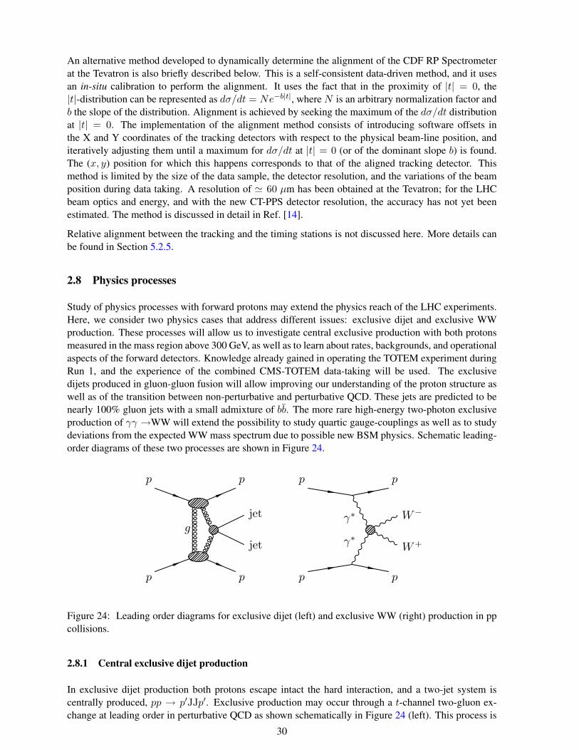
An alternative method developed to dynamically determine the alignment of the CDF RP Spectrometerat the Tevatron is also briefly described below. This is a self-consistent data-driven method, and it usesan in-situ calibration to perform the alignment. It uses the fact that in the proximity of |t| = 0, the|t|-distribution can be represented as dσ/dt = Ne−b|t|, where N is an arbitrary normalization factor andb the slope of the distribution. Alignment is achieved by seeking the maximum of the dσ/dt distributionat |t| = 0. The implementation of the alignment method consists of introducing software offsets inthe X and Y coordinates of the tracking detectors with respect to the physical beam-line position, anditeratively adjusting them until a maximum for dσ/dt at |t| = 0 (or of the dominant slope b) is found.The (x, y) position for which this happens corresponds to that of the aligned tracking detector. Thismethod is limited by the size of the data sample, the detector resolution, and the variations of the beamposition during data taking. A resolution of ' 60 µm has been obtained at the Tevatron; for the LHCbeam optics and energy, and with the new CT-PPS detector resolution, the accuracy has not yet beenestimated. The method is discussed in detail in Ref. [14].

Relative alignment between the tracking and the timing stations is not discussed here. More details canbe found in Section 5.2.5.

2.8 Physics processes

Study of physics processes with forward protons may extend the physics reach of the LHC experiments.Here, we consider two physics cases that address different issues: exclusive dijet and exclusive WWproduction. These processes will allow us to investigate central exclusive production with both protonsmeasured in the mass region above 300 GeV, as well as to learn about rates, backgrounds, and operationalaspects of the forward detectors. Knowledge already gained in operating the TOTEM experiment duringRun 1, and the experience of the combined CMS-TOTEM data-taking will be used. The exclusivedijets produced in gluon-gluon fusion will allow improving our understanding of the proton structure aswell as of the transition between non-perturbative and perturbative QCD. These jets are predicted to benearly 100% gluon jets with a small admixture of bb. The more rare high-energy two-photon exclusiveproduction of γγ →WW will extend the possibility to study quartic gauge-couplings as well as to studydeviations from the expected WW mass spectrum due to possible new BSM physics. Schematic leading-order diagrams of these two processes are shown in Figure 24.

g

p

p

p

jet

jet

p

γ∗

γ∗

p

p

p

W+

W−

p

Figure 24: Leading order diagrams for exclusive dijet (left) and exclusive WW (right) production in ppcollisions.

2.8.1 Central exclusive dijet production

In exclusive dijet production both protons escape intact the hard interaction, and a two-jet system iscentrally produced, pp → p′JJp′. Exclusive production may occur through a t-channel two-gluon ex-change at leading order in perturbative QCD as shown schematically in Figure 24 (left). This process is

30

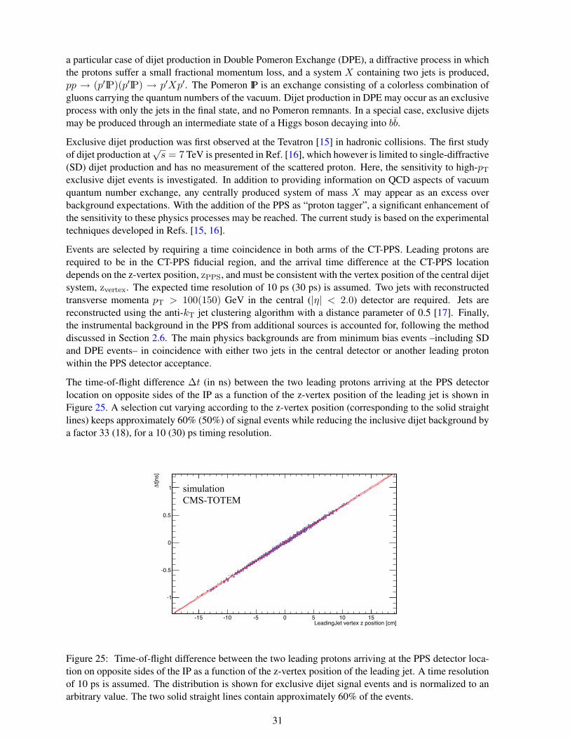
a particular case of dijet production in Double Pomeron Exchange (DPE), a diffractive process in whichthe protons suffer a small fractional momentum loss, and a system X containing two jets is produced,pp → (p′IP)(p′IP) → p′Xp′. The Pomeron IP is an exchange consisting of a colorless combination ofgluons carrying the quantum numbers of the vacuum. Dijet production in DPE may occur as an exclusiveprocess with only the jets in the final state, and no Pomeron remnants. In a special case, exclusive dijetsmay be produced through an intermediate state of a Higgs boson decaying into bb.

Exclusive dijet production was first observed at the Tevatron [15] in hadronic collisions. The first studyof dijet production at

√s = 7 TeV is presented in Ref. [16], which however is limited to single-diffractive

(SD) dijet production and has no measurement of the scattered proton. Here, the sensitivity to high-pT

exclusive dijet events is investigated. In addition to providing information on QCD aspects of vacuumquantum number exchange, any centrally produced system of mass X may appear as an excess overbackground expectations. With the addition of the PPS as “proton tagger”, a significant enhancement ofthe sensitivity to these physics processes may be reached. The current study is based on the experimentaltechniques developed in Refs. [15, 16].

Events are selected by requiring a time coincidence in both arms of the CT-PPS. Leading protons arerequired to be in the CT-PPS fiducial region, and the arrival time difference at the CT-PPS locationdepends on the z-vertex position, zPPS, and must be consistent with the vertex position of the central dijetsystem, zvertex. The expected time resolution of 10 ps (30 ps) is assumed. Two jets with reconstructedtransverse momenta pT > 100(150) GeV in the central (|η| < 2.0) detector are required. Jets arereconstructed using the anti-kT jet clustering algorithm with a distance parameter of 0.5 [17]. Finally,the instrumental background in the PPS from additional sources is accounted for, following the methoddiscussed in Section 2.6. The main physics backgrounds are from minimum bias events –including SDand DPE events– in coincidence with either two jets in the central detector or another leading protonwithin the PPS detector acceptance.

The time-of-flight difference ∆t (in ns) between the two leading protons arriving at the PPS detectorlocation on opposite sides of the IP as a function of the z-vertex position of the leading jet is shown inFigure 25. A selection cut varying according to the z-vertex position (corresponding to the solid straightlines) keeps approximately 60% (50%) of signal events while reducing the inclusive dijet background bya factor 33 (18), for a 10 (30) ps timing resolution.

LeadingJet vertex z position [cm]-15 -10 -5 0 5 10 15

t[ns]

Δ

-1

-0.5

0

0.5

1 simulation CMS-TOTEM

Figure 25: Time-of-flight difference between the two leading protons arriving at the PPS detector loca-tion on opposite sides of the IP as a function of the z-vertex position of the leading jet. A time resolutionof 10 ps is assumed. The distribution is shown for exclusive dijet signal events and is normalized to anarbitrary value. The two solid straight lines contain approximately 60% of the events.

31

Kinematic distributions after the PPS tagging selection are shown in Figure 26. The leading jet pT

and the azimuthal angle difference between the two leading jets are shown for signal and backgroundevents. The dijet invariant mass Mjj and the missing mass MX =

√s · ξ1 · ξ2 are also shown. MX is

estimated from the reconstructed fractional momentum loss values of the two leading protons, ξ1 and ξ2.Figure 27 (left) shows the dijet mass fraction, Rjj = Mjj/MX, and the rapidity difference (right) of thejet system (yjj) and the proton system, yX = 0.5 · ln(ξ1/ξ2). Consistency is required between the valuesof the jet mass system measured in the central detector (Mjj) and in the PPS (MX), and the requirement0.70 < Rjj < 1.15 is applied. A selection cut of |(yjj − yX)| < 0.1 is also required.

[GeV]T

Leading Jet p100 150 200 250 300 350 400 450

Arbi

trary

uni

t

0

0.02

0.04

0.06

0.08

0.1ExhumePomwig DPE Pomwig SDPythia8 QCD


jjφΔ

0 0.5 1 1.5 2 2.5 3

Arbi

trary

uni

t-310

-210

-110

ExhumePomwig DPE Pomwig SDPythia8 QCD


[GeV]jj M200 400 600 800 1000 1200

Arbi

trary

uni

t

0

0.05

0.1

0.15

0.2

0.25

0.3

0.35 ExhumePomwig DPE Pomwig SDPythia8 QCD


[GeV]x M200 400 600 800 1000 1200 1400 1600 1800 2000

Arbi

trary

uni

t

0

0.05

0.1

0.15

0.2



Figure 26: Leading jet pT (top, left), azimuthal angle difference between the two leading jets (top, right),dijet invariant massMjj (bottom, left), and the missing massMX =

√s · ξ1 · ξ2 (bottom, right) estimated

from the reconstructed values of the two leading protons, ξ1 and ξ2. Distributions are shown for exclusivedijet signal (ExHuME) and for background (SD, DPE, inclusive dijets) events, and are normalized to unitarea.

The track multiplicity associated to the dijet vertex is used to discriminate exclusive signal events againstbackgrounds. In particular, we exploit techniques developed in Ref. [18]. We build two variables thataccount for the “exclusitivity” of the event by counting the number of extra tracks between the jets, bothin φ and η. We call these variables Nφ

tracks and Nηtracks. Figure 28 shows a sketch of the central detector

coverage with the two jets (dark shaded circles), and the areas between them that are used to count the

32

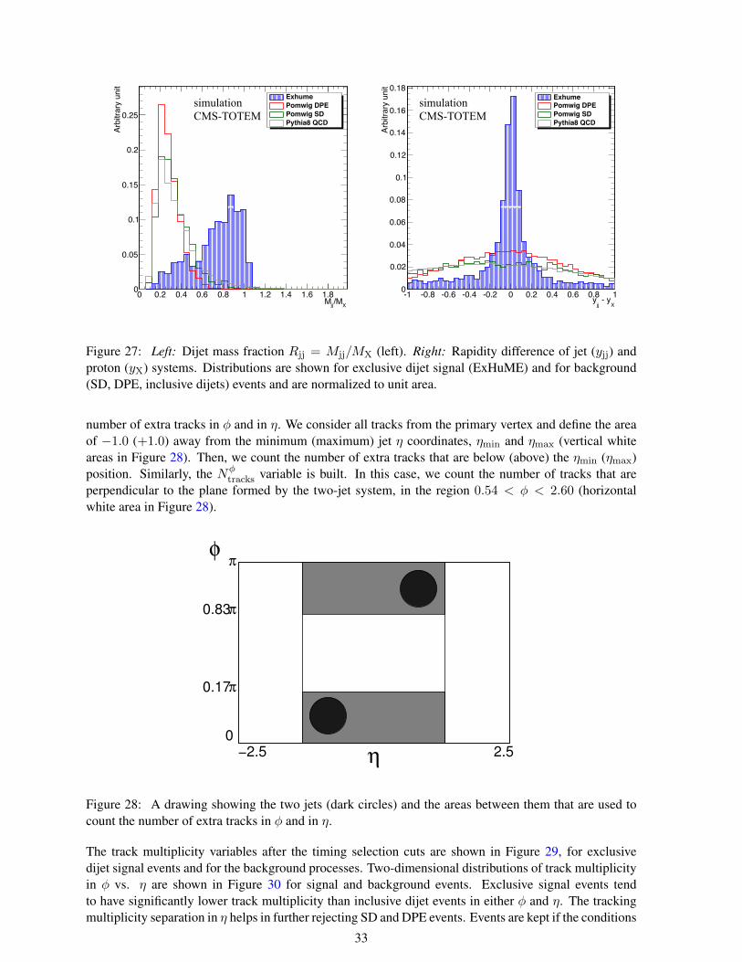
X/Mjj M0 0.2 0.4 0.6 0.8 1 1.2 1.4 1.6 1.8

Arbi

trary

uni

t

0

0.05

0.1

0.15

0.2

0.25



X - y

jj y-1 -0.8 -0.6 -0.4 -0.2 0 0.2 0.4 0.6 0.8 1

Arbi

trary

uni

t

0

0.02

0.04

0.06

0.08

0.1

0.12

0.14

0.16



Figure 27: Left: Dijet mass fraction Rjj = Mjj/MX (left). Right: Rapidity difference of jet (yjj) andproton (yX) systems. Distributions are shown for exclusive dijet signal (ExHuME) and for background(SD, DPE, inclusive dijets) events and are normalized to unit area.

number of extra tracks in φ and in η. We consider all tracks from the primary vertex and define the areaof −1.0 (+1.0) away from the minimum (maximum) jet η coordinates, ηmin and ηmax (vertical whiteareas in Figure 28). Then, we count the number of extra tracks that are below (above) the ηmin (ηmax)position. Similarly, the Nφ

tracks variable is built. In this case, we count the number of tracks that areperpendicular to the plane formed by the two-jet system, in the region 0.54 < φ < 2.60 (horizontalwhite area in Figure 28).

π

2.5−2.5

0

π

π0.83

0.17

φ

η

Figure 28: A drawing showing the two jets (dark circles) and the areas between them that are used tocount the number of extra tracks in φ and in η.

The track multiplicity variables after the timing selection cuts are shown in Figure 29, for exclusivedijet signal events and for the background processes. Two-dimensional distributions of track multiplicityin φ vs. η are shown in Figure 30 for signal and background events. Exclusive signal events tendto have significantly lower track multiplicity than inclusive dijet events in either φ and η. The trackingmultiplicity separation in η helps in further rejecting SD and DPE events. Events are kept if the conditions

33

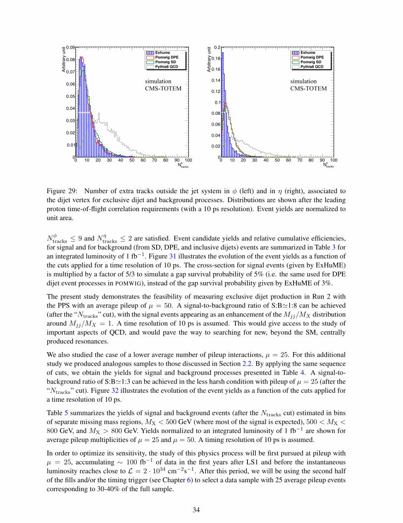
φ

tracksN0 10 20 30 40 50 60 70 80 90 100

Arbi

trary

uni

t

0

0.01

0.02

0.03

0.04

0.05

0.06

0.07

0.08



η

tracks N0 10 20 30 40 50 60 70 80 90 100

Arbi

trary

uni

t

0

0.02

0.04

0.06

0.08

0.1

0.12

0.14

0.16

0.18



Figure 29: Number of extra tracks outside the jet system in φ (left) and in η (right), associated tothe dijet vertex for exclusive dijet and background processes. Distributions are shown after the leadingproton time-of-flight correlation requirements (with a 10 ps resolution). Event yields are normalized tounit area.

Nφtracks ≤ 9 and Nη

tracks ≤ 2 are satisfied. Event candidate yields and relative cumulative efficiencies,for signal and for background (from SD, DPE, and inclusive dijets) events are summarized in Table 3 foran integrated luminosity of 1 fb−1. Figure 31 illustrates the evolution of the event yields as a function ofthe cuts applied for a time resolution of 10 ps. The cross-section for signal events (given by ExHuME)is multiplied by a factor of 5/3 to simulate a gap survival probability of 5% (i.e. the same used for DPEdijet event processes in POMWIG), instead of the gap survival probability given by ExHuME of 3%.

The present study demonstrates the feasibility of measuring exclusive dijet production in Run 2 withthe PPS with an average pileup of µ = 50. A signal-to-background ratio of S:B'1:8 can be achieved(after the “Ntracks” cut), with the signal events appearing as an enhancement of theMjj/MX distributionaround Mjj/MX = 1. A time resolution of 10 ps is assumed. This would give access to the study ofimportant aspects of QCD, and would pave the way to searching for new, beyond the SM, centrallyproduced resonances.

We also studied the case of a lower average number of pileup interactions, µ = 25. For this additionalstudy we produced analogous samples to those discussed in Section 2.2. By applying the same sequenceof cuts, we obtain the yields for signal and background processes presented in Table 4. A signal-to-background ratio of S:B'1:3 can be achieved in the less harsh condition with pileup of µ = 25 (after the“Ntracks” cut). Figure 32 illustrates the evolution of the event yields as a function of the cuts applied fora time resolution of 10 ps.

Table 5 summarizes the yields of signal and background events (after the Ntracks cut) estimated in binsof separate missing mass regions, MX < 500 GeV (where most of the signal is expected), 500 < MX <800 GeV, and MX > 800 GeV. Yields normalized to an integrated luminosity of 1 fb−1 are shown foraverage pileup multiplicities of µ = 25 and µ = 50. A timing resolution of 10 ps is assumed.

In order to optimize its sensitivity, the study of this physics process will be first pursued at pileup withµ = 25, accumulating ∼ 100 fb−1 of data in the first years after LS1 and before the instantaneousluminosity reaches close to L = 2 · 1034 cm−2s−1. After this period, we will be using the second halfof the fills and/or the timing trigger (see Chapter 6) to select a data sample with 25 average pileup eventscorresponding to 30-40% of the full sample.

34

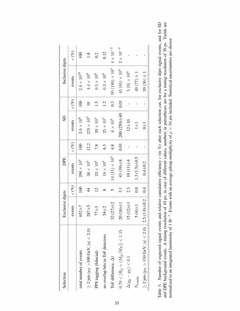
Sele

ctio

nE

xclu

sive

dije

tsD

PESD

Incl

usiv

edi

jets

even

tsε

(%)

even

tsε

(%)

even

tsε

(%)

even

tsε

(%)

tota

lnum

bero

feve

nts

652±

710

029

0×

103

100

2.6×

106

100

2.4×

1010

100

≥2

jets

(pT>

100

GeV

,|η|<

2.0)

287±

544

36×

103

12.2

270×

103

104.

4×

108

1.8

PPS

tagg

ing

(fidu

cial

)77±

312

23×

103

7.8

39×

103

1.5

0.5×

108

0.2

noov

erla

phi

tsin

ToF

dete

ctor

s54±

28

18×

103

6.3

25×

103

1.2

0.3×

108

0.12

ToF

diff

eren

ce,∆

t32

(27)±

25

14(1

1)×

103

4.8

6×

103

0.3

95(1

80)×

104

4×

10−

3

0.70<

[Rjj

=(M

jj/M

X)]<

1.15

20(1

6)±

13.

143

(39)±

80.

0120

0(2

50)±

400.

0145

(85)×

103

2×

10−

4

∆(y

jj−y X

)<

0.1

15(1

2)±

12.

310

(11)±

4-

12±

10-

5(9

)×

103

-

Ntr

ack

s5

(4)±

10.

81.

3(1

.5)±

0.5

-1±

1-

40(7

7)±

1-

≥2

jets

(pT>

150

GeV

,|η|<

2.0)

2.5

(1.9

)±0.

20.

40.

4±0.

2-

0±1

-20

(36)±

1-

Tabl

e3:

Num

ber

ofex

pect

edsi

gnal

even

tsan

dre

lativ

ecu

mul

ativ

eef

ficie

ncyε

(in

%)

afte

rea

chse

lect

ion

cut,

for

excl

usiv

edi

jet

sign

alev

ents

,an

dfo

rSD

and

DPE

back

grou

ndev

ents

.A

timin

gre

solu

tion

of10

ps;

inca

seof

diff

eren

tval

ues,

num

bers

inpa

rent

hese

sar

efo

ra

timin

gre

solu

tion

of30

ps.

Yie

lds

are

norm

aliz

edto

anin

tegr

ated

lum

inos

ityof

1fb−

1.E

vent

sw

ithan

aver

age

pile

upm

ultip

licity

ofµ

=50

are

incl

uded

.Sta

tistic

alun

cert

aint

ies

are

show

n.

35

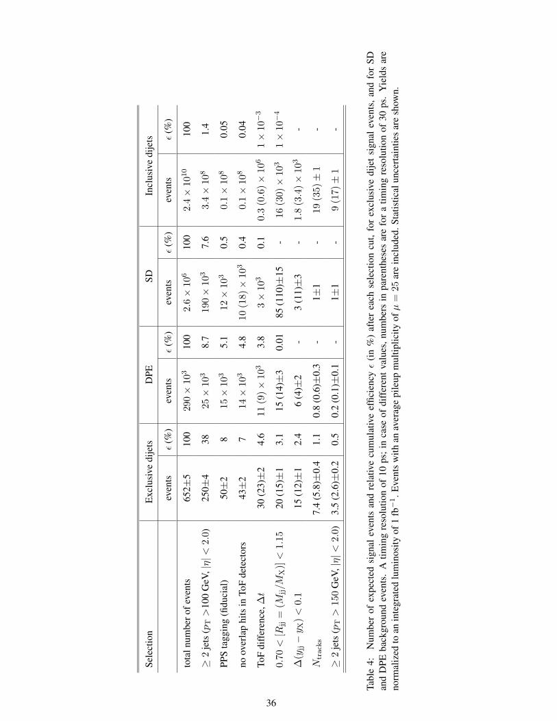
Sele

ctio

nE

xclu

sive

dije

tsD

PESD

Incl

usiv

edi

jets

even

tsε

(%)

even

tsε

(%)

even

tsε

(%)

even

tsε

(%)

tota

lnum

bero

feve

nts

652±

510

029

0×

103

100

2.6×

106

100

2.4×

1010

100

≥2

jets

(pT>

100

GeV

,|η|<

2.0)

250±

438

25×

103

8.7

190×

103

7.6

3.4×

108

1.4

PPS

tagg

ing

(fidu

cial

)50±

28

15×

103

5.1

12×

103

0.5

0.1×

108

0.05

noov

erla

phi

tsin

ToF

dete

ctor

s43±

27

14×

103

4.8

10(1

8)×

103

0.4

0.1×

108

0.04

ToF

diff

eren

ce,∆

t30

(23)±

24.

611

(9)×

103

3.8

3×

103

0.1

0.3

(0.6

)×

106

1×

10−

3

0.70<

[Rjj

=(M

jj/M

X)]<

1.15

20(1

5)±

13.

115

(14)±

30.

0185

(110

)±15

-16

(30)×

103

1×

10−

4

∆(y

jj−y X

)<

0.1

15(1

2)±

12.

46

(4)±

2-

3(1

1)±

3-

1.8

(3.4

)×

103

-

Ntr

ack

s7.

4(5

.8)±

0.4

1.1

0.8

(0.6

)±0.

3-

1±1

-19

(35)±

1-

≥2

jets

(pT>

150

GeV

,|η|<

2.0)

3.5

(2.6

)±0.

20.

50.

2(0

.1)±

0.1

-1±

1-

9(1

7)±

1-

Tabl

e4:

Num

ber

ofex

pect

edsi

gnal

even

tsan

dre

lativ

ecu

mul

ativ

eef

ficie

ncyε

(in

%)

afte

rea

chse

lect

ion

cut,

for

excl

usiv

edi

jet

sign

alev

ents

,an

dfo

rSD

and

DPE

back

grou

ndev

ents

.A

timin

gre

solu

tion

of10

ps;

inca

seof

diff

eren

tval

ues,

num

bers

inpa

rent

hese

sar

efo

ra

timin

gre

solu

tion

of30

ps.

Yie

lds

are

norm

aliz

edto

anin

tegr

ated

lum

inos

ityof

1fb−

1.E

vent

sw

ithan

aver

age

pile

upm

ultip

licity

ofµ

=25

are

incl

uded

.Sta

tistic

alun

cert

aint

ies

are

show

n.

36

φ Nxtracks 0 5 10 15 20 25 30

η N

xtra

cks

0

5

10

15

20

25

30


Nxtracks Phi0 5 10 15 20 25 30

Nxt

rack

s Et

a

0

5

10

15

20

25

30


Nxtracks Phi0 5 10 15 20 25 30

Nxt

rack

s Et

a

0

5

10

15

20

25

30


φ Nxtracks 0 5 10 15 20 25 30

η N

xtra

cks

0

5

10

15

20

25

30simulation CMS-TOTEM

Figure 30: Number of extra tracks in φ vs η for exclusive signal events (top, left), inclusive dijet (top,right), SD (bottom, left), and DPE (bottom, right) events. Distributions are shown after the leading protontime-of-flight correlation requirements (with a 10 ps resolution), and are normalized to unit area.

Exclusive dijets DPE SD Inclusive dijets S:B

pileup µ = 25

MX ≤ 500 GeV 4.0±0.2 0.2±0.1 0±1 1± 1 3:1

500 < MX ≤ 800 GeV 3.1±0.2 0.3±0.1 0±1 15± 1 1:5

MX > 800 GeV 0.3±0.1 0.3±0.1 1±1 4± 1 1:18

pileup µ = 50

MX ≤ 500 GeV 2.8±0.2 0.6±0.2 0±1 5± 1 1:2

500 < MX ≤ 800 GeV 2.3±0.2 0.7±0.3 1.3±1.0 26± 1 1:12

MX > 800 GeV 0.3±0.1 0±1 0±1 9± 1 1:30

Table 5: Number of expected signal and background (SD, DPE, and inclusive dijets) events (after theNtracks cut), for separate bins of missing mass MX. Yields normalized to an integrated luminosity of1 fb−1 are shown for average pileup multiplicities of µ = 25 and µ = 50. Statistical uncertainties areshown. A timing resolution of 10 ps is assumed.

37

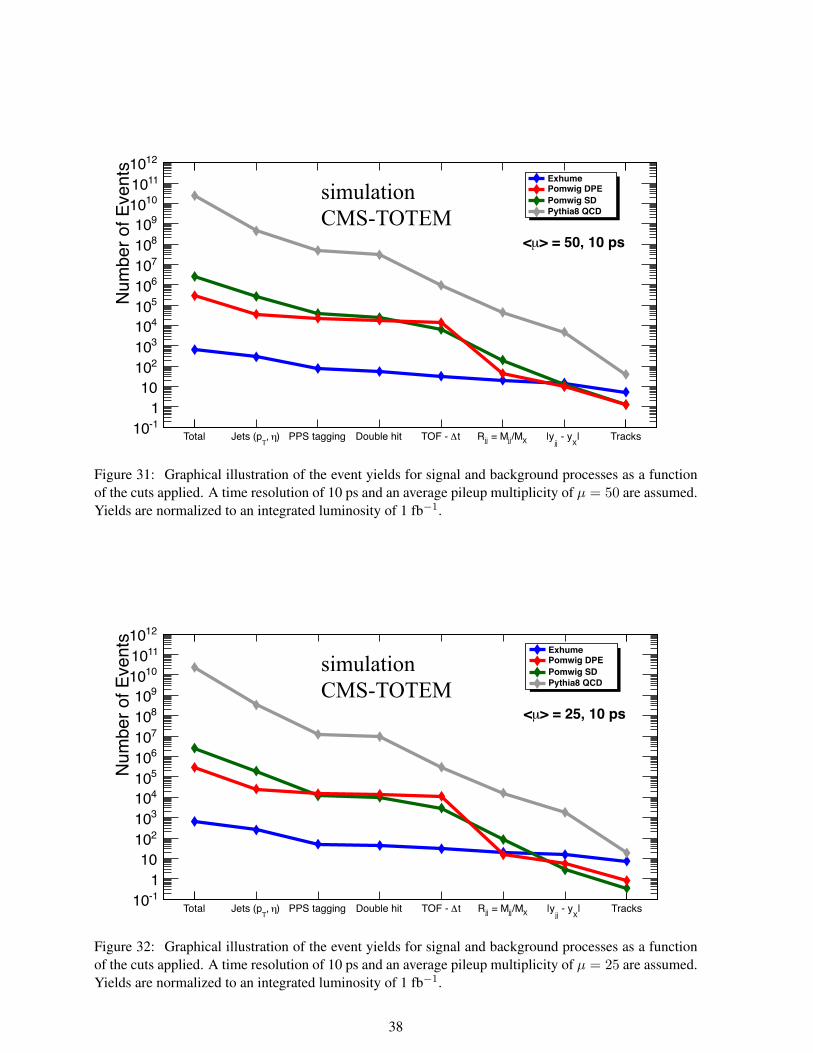
Total )η, T

Jets (p PPS tagging Double hit tΔTOF - X/Mjj = MjjR | X

- yjj

|y Tracks

Num

ber o

f Eve

nts

-1101

10210

310410510

610710

810

910101011101210


> = 50, 10 psµ<


Figure 31: Graphical illustration of the event yields for signal and background processes as a functionof the cuts applied. A time resolution of 10 ps and an average pileup multiplicity of µ = 50 are assumed.Yields are normalized to an integrated luminosity of 1 fb−1.

Total )η, T

Jets (p PPS tagging Double hit tΔTOF - X/Mjj = MjjR | X

- yjj

|y Tracks

Num

ber o

f Eve

nts

-1101

10210

310410510

610710

810

910101011101210


> = 25, 10 psµ<


Figure 32: Graphical illustration of the event yields for signal and background processes as a functionof the cuts applied. A time resolution of 10 ps and an average pileup multiplicity of µ = 25 are assumed.Yields are normalized to an integrated luminosity of 1 fb−1.

38

2.8.2 Central exclusive WW production

The study of high-energy photon interactions at the LHC opens up the possibility of interesting andnovel research [19, 20]. In particular, measurements of the two-photon production of a pair of W-bosonsprovide sensitivity to anomalous quartic gauge couplings of the gauge bosons. Measurements of theexclusive two-photon production of W boson pairs, in the process pp → pW+W−p, were performed inthe µ±e∓ final state, using 5.05 fb−1 of data collected in proton-proton collisions at

√s = 7 TeV with the

CMS detector at the LHC in 2011, but without the proton tagging [21]. Model-independent upper limitswere extracted and compared to predictions involving anomalous quartic gauge couplings (AQGCs).

The current study is based on the experimental techniques developed in Ref. [21]. With the integratedluminosity expected to be collected during Run 2 and with the CT-PPS detectors, the experimental reachcan be extended by several orders of magnitude with respect to the best limits obtained so far. In theprocess pp → pWWp, both forward-scattered protons are detected in the CT-PPS, depending on theacceptance on the mass of the WW central system produced (Figure 17). The CT-PPS detector is assumedto be at 15 σ from the beam (including the dead region of 0.3 mm due to the RP window).

This process is characterized by a primary vertex from the two leptons `±`′∓ (where ` = e, µ) from theW boson pair decays, no other track, a large transverse momentum of the dilepton system, pT(`±`′∓),and a large invariant mass, M(`±`′∓). A simulated sample of SM exclusive pp → pWWp signalevents is used, in conjunction with samples in which anomalous quartic gauge couplings (AQGC) areassumed. The dominant SM backgrounds come from inclusive W+W− and exclusive τ+τ− pair pro-duction. Drell-Yan (DY) production of τ+τ−, where one τ decays via the electron channel and the otherone via the muon channel, in combination with pileup protons, may lead to a similar event configu-ration as the exclusive WW signal. A selection cut on the transverse momentum of the dilepton pairpT (`±`′∓) > 30 GeV was used in Ref. [21] to reject the DY background almost completely. A furtherrejection of the other SM backgrounds, and a reduction of signal events by approximately 20% is ex-pected. In this study, only the eµ final state is selected. The inclusion of same-flavor channels (ee andµµ) will also be addressed as it brings an enhancement in sensitivity. However, in this case the gain canbe mitigated as, in order to reduce the background from DY processes, additional selection cuts may benecessary.

The simulated samples for the signal process are compared to the SM background expectations. Tailsof the MX distribution (MX =

√s · ξ1 · ξ2 > 1 TeV), where the SM γγ → W+W− contribution

is expected to be small, are investigated to look for AQGCs. Events are selected by requiring twocentral (|η| < 2.4) leptons with a minimum transverse momentum pT > 20 GeV. In order to reducethe contamination from the W+jet (or other non-prompt lepton) background, “tight” lepton identificationcriteria are imposed (as in Ref. [21]). Leptons are also required to have charges of opposite sign andto come from the same primary vertex. For signal events (either SM or AQGC), the scattered protonsare in the region covered by CT-PPS, and the presence of hits in both tracking and timing detectors istherefore required: a large background suppression is expected. A source of inefficiency comes fromdetector segmentation, as hits are required not to overlap in the timing detector cells.

Signal events from SM exclusive WW events are correlated in time with the leading protons detected inthe CT-PPS detectors, whereas inclusive WW events -superimposed with additional pileup events- arenot. Therefore, the information of the proton time-of-flight arrival at the CT-PPS detector location canbe used as an additional background rejection. After requiring the coincidence of hits in both trackingand timing detector stations, the time-of-flight difference between the two leading protons arriving at theCT-PPS detector location on opposite sides of the IP is shown in Figure 33 as a function of the z-vertexposition of the leading central lepton, for signal (left) and background (right) events. For each event,if there is more than one pp combination in the CT-PPS detector, only the one with the closest matchbetween the time-of-flight ∆t and the lepton vertex position in z is kept (“vertex matching” in Table 6).The background is shown for inclusive WW events in coincidence with pileup events. Distributions cor-

39

responding to timing resolutions of 10 ps (top) and 30 ps (bottom) are shown for signal and backgroundevents.

Leading lepton vertex z position [cm]-25 -20 -15 -10 -5 0 5 10 15 20 25

-t [n

s]Δ

ToF

-1

-0.8

-0.6

-0.4

-0.2

0

0.2

0.4

0.6

0.8

1WW, both protons from signal→γγ



-t [n

s]Δ

ToF

-1

-0.8

-0.6

-0.4

-0.2

0

0.2

0.4

0.6

0.8

1Inclusive WW background



-t [n

s]Δ

ToF

-1

-0.8

-0.6

-0.4

-0.2

0

0.2

0.4

0.6

0.8

1WW, both protons from signal→γγ



-t [n

s]Δ

ToF

-1

-0.8

-0.6

-0.4

-0.2

0

0.2

0.4

0.6

0.8

1Inclusive WW background


Figure 33: Time-of-flight difference between the two leading protons arriving at the CT-PPS detectorlocation on opposite sides of the IP as a function of the z-vertex position of the leading central leptonfor exclusive signal (left) and background inclusive WW (right) events. Timing resolutions of 10 ps(top) and 30 ps (bottom) are assumed. Distributions are shown for events where both leading protons arewithin the CT-PPS detector acceptance (after selecting the closest match of the vertices of the dileptonsystem and of the leading protons), and before the time-of-flight difference requirement. The dotted linesshow an ideal window retaining close to 100% of signal events. An arbitrary normalization is used in thedistributions.

The distance (in z) of the vertex positions measured from the CT-PPS timing detectors and from theleading lepton in the central detector, ∆z = zPPS − zlead lep, is shown in Figure 34 for SM exclusiveWW/ττ and inclusive WW events, and for AQGC exclusive WW events. Time-of-flight requirementsmay help reducing the inclusive WW background by a factor of 10 (5), for a timing resolution of 10 ps(30 ps).

The track multiplicity associated to the dilepton vertex after the timing selection cuts is shown in Fig-ure 35 for SM signal and backgrounds. The number of extra tracks associated to the dilepton vertex is

40

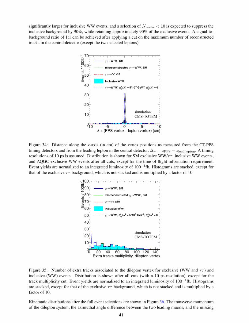
significantly larger for inclusive WW events, and a selection of Ntracks < 10 is expected to suppress theinclusive background by 90%, while retaining approximately 90% of the exclusive events. A signal-to-background ratio of 1:1 can be achieved after applying a cut on the maximum number of reconstructedtracks in the central detector (except the two selected leptons).

z (PPS vertex - lepton vertex) [cm]Δ-10 -5 0 5 10

-1Ev

ents

/ 10

0fb

0

10

20

30

40

50

60

70, SM-W+W→γγ

, SM-W+W→γγmisreconstructed

x10-τ+τ→γγ

-W+Inclusive W

= 02Λ/WC, a-2 GeV-6 = 5*102Λ/

W0, a-W+W→γγ


Figure 34: Distance along the z-axis (in cm) of the vertex positions as measured from the CT-PPStiming detectors and from the leading lepton in the central detector, ∆z = zPPS − zlead lepton. A timingresolutions of 10 ps is assumed. Distribution is shown for SM exclusive WW/ττ , inclusive WW events,and AQGC exclusive WW events after all cuts, except for the time-of-flight information requirement.Event yields are normalized to an integrated luminosity of 100−1fb. Histograms are stacked, except forthat of the exclusive ττ background, which is not stacked and is multiplied by a factor of 10.

Extra tracks multiplicity, dilepton vertex0 20 40 60 80 100 120 140

-1Ev

ents

/ 10

0fb

0102030405060708090

100, SM-W+W→γγ


x10-τ+τ→γγ

-W+Inclusive W

= 02Λ/WC, a-2 GeV-6 = 5*102Λ/

W0, a-W+W→γγ


Figure 35: Number of extra tracks associated to the dilepton vertex for exclusive (WW and ττ ) andinclusive (WW) events. Distribution is shown after all cuts (with a 10 ps resolution), except for thetrack multiplicity cut. Event yields are normalized to an integrated luminosity of 100−1fb. Histogramsare stacked, except for that of the exclusive ττ background, which is not stacked and is multiplied by afactor of 10.

Kinematic distributions after the full event selections are shown in Figure 36. The transverse momentumof the dilepton system, the azimuthal angle difference between the two leading muons, and the missing

41

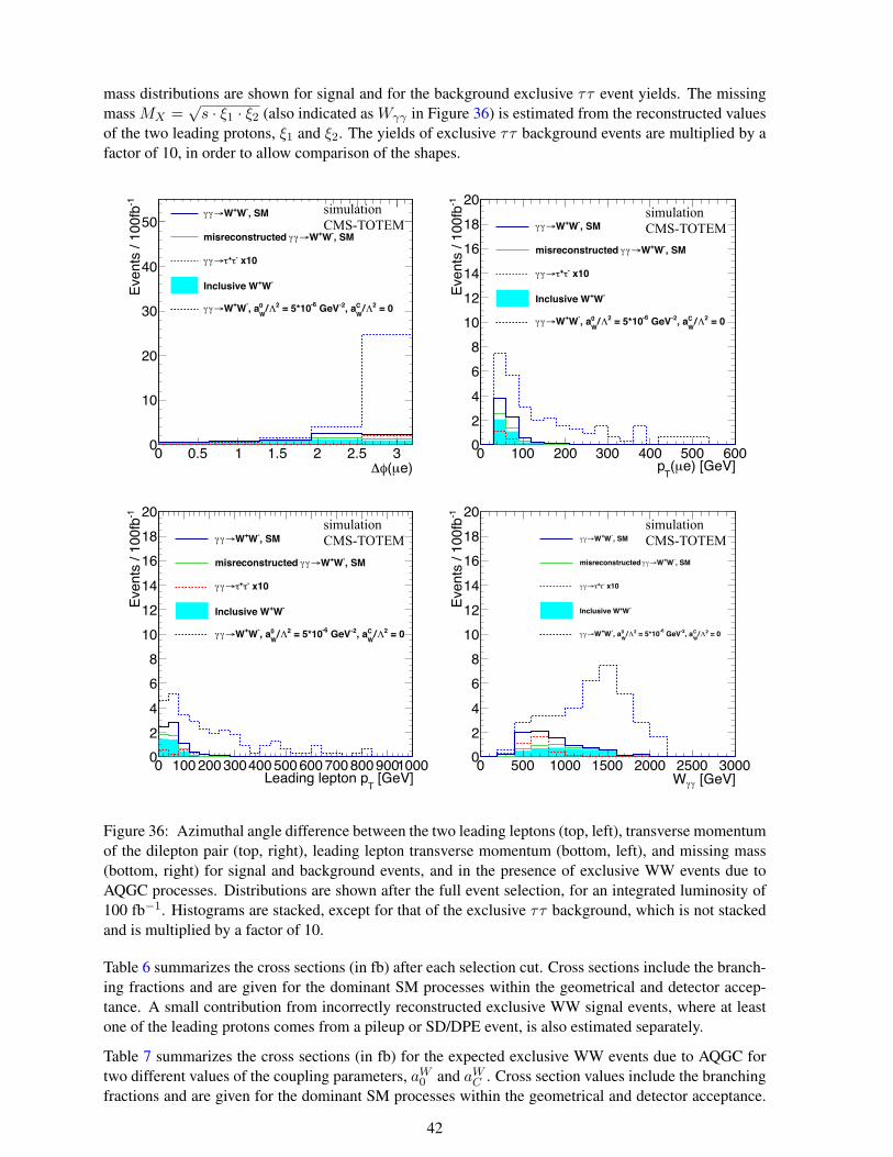
mass distributions are shown for signal and for the background exclusive ττ event yields. The missingmass MX =

√s · ξ1 · ξ2 (also indicated as Wγγ in Figure 36) is estimated from the reconstructed values

of the two leading protons, ξ1 and ξ2. The yields of exclusive ττ background events are multiplied by afactor of 10, in order to allow comparison of the shapes.

e)µ(φΔ0 0.5 1 1.5 2 2.5 3

-1Ev

ents

/ 10

0fb

0

10

20

30

40

50, SM-W+W→γγ


x10-τ+τ→γγ

-W+Inclusive W

= 02Λ/WC, a-2 GeV-6 = 5*102Λ/

W0, a-W+W→γγ


e) [GeV]µ(T

p0 100 200 300 400 500 600

-1Ev

ents

/ 10

0fb

02468

101214161820

, SM-W+W→γγ


x10-τ+τ→γγ

-W+Inclusive W

= 02Λ/WC, a-2 GeV-6 = 5*102Λ/

W0, a-W+W→γγ


[GeV]T

Leading lepton p0 100 200 300400 500 600 700 800 9001000

-1Ev

ents

/ 10

0fb

02468

101214161820

, SM-W+W→γγ


x10-τ+τ→γγ

-W+Inclusive W

= 02Λ/WC, a-2 GeV-6 = 5*102Λ/

W0, a-W+W→γγ


[GeV]γγW0 500 1000 1500 2000 2500 3000

-1Ev

ents

/ 10

0fb

02468

101214161820

, SM-W+W→γγ


x10-τ+τ→γγ

-W+Inclusive W

= 02Λ/WC, a-2 GeV-6 = 5*102Λ/

W0, a-W+W→γγ


Figure 36: Azimuthal angle difference between the two leading leptons (top, left), transverse momentumof the dilepton pair (top, right), leading lepton transverse momentum (bottom, left), and missing mass(bottom, right) for signal and background events, and in the presence of exclusive WW events due toAQGC processes. Distributions are shown after the full event selection, for an integrated luminosity of100 fb−1. Histograms are stacked, except for that of the exclusive ττ background, which is not stackedand is multiplied by a factor of 10.

Table 6 summarizes the cross sections (in fb) after each selection cut. Cross sections include the branch-ing fractions and are given for the dominant SM processes within the geometrical and detector accep-tance. A small contribution from incorrectly reconstructed exclusive WW signal events, where at leastone of the leading protons comes from a pileup or SD/DPE event, is also estimated separately.

Table 7 summarizes the cross sections (in fb) for the expected exclusive WW events due to AQGC fortwo different values of the coupling parameters, aW

0 and aWC . Cross section values include the branching

fractions and are given for the dominant SM processes within the geometrical and detector acceptance.

42

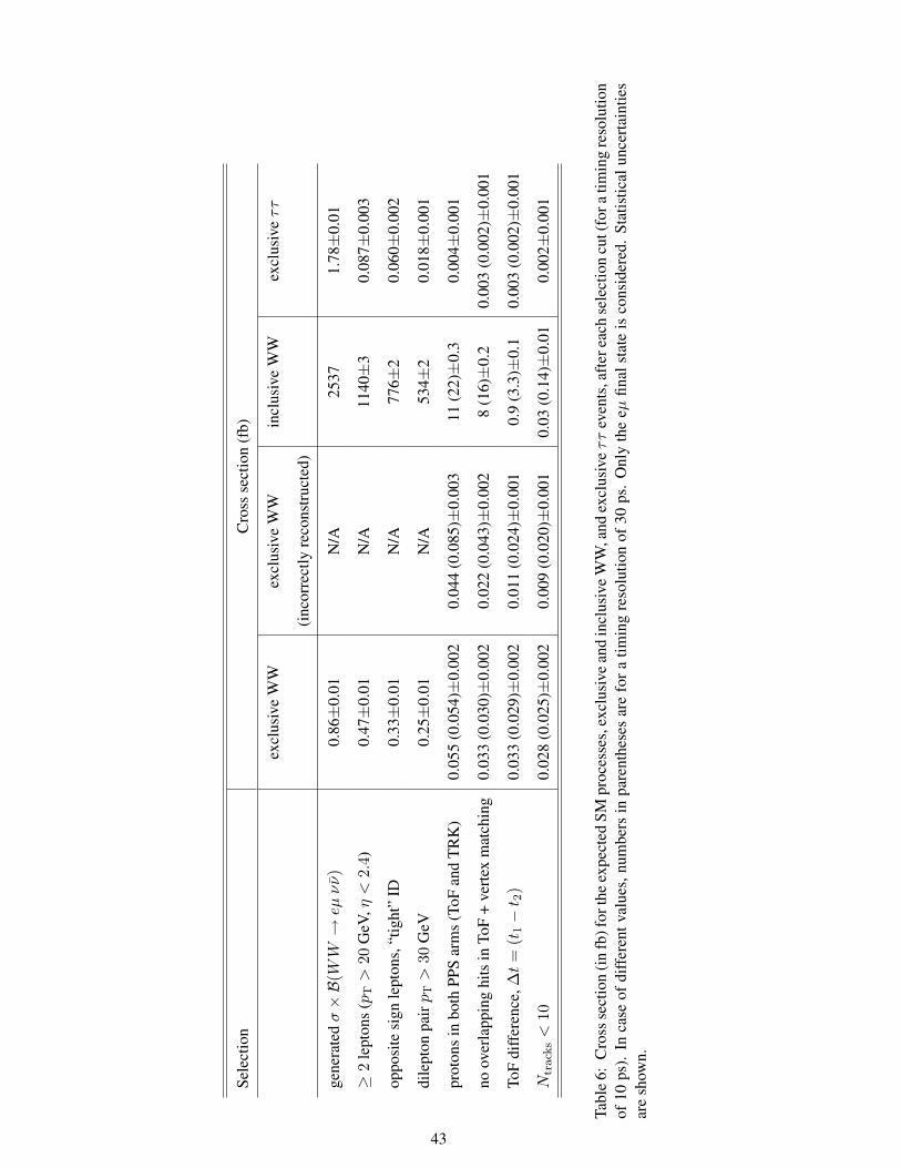
Sele

ctio

nC

ross

sect

ion

(fb)

excl

usiv

eW

Wex

clus

ive

WW

incl

usiv

eW

Wex

clus

iveττ

(inc

orre

ctly

reco

nstr

ucte

d)

gene

rate

dσ×B

(WW→eµ

νν)

0.86±

0.01

N/A

2537

1.78±

0.01

≥2

lept

ons

(pT>

20G

eV,η

<2.

4)0.

47±

0.01

N/A

1140±

30.

087±

0.00

3

oppo

site

sign

lept

ons,

“tig

ht”

ID0.

33±

0.01

N/A

776±

20.

060±

0.00

2

dile

pton

pairpT>

30G

eV0.

25±

0.01

N/A

534±

20.

018±

0.00

1

prot

ons

inbo

thPP

Sar

ms

(ToF

and

TR

K)

0.05

5(0

.054

)±0.

002

0.04

4(0

.085

)±0.

003

11(2

2)±

0.3

0.00

4±0.

001

noov

erla

ppin

ghi

tsin

ToF

+ve

rtex

mat

chin

g0.

033

(0.0

30)±

0.00

20.

022

(0.0

43)±

0.00

28

(16)±

0.2

0.00

3(0

.002

)±0.

001

ToF

diff

eren

ce,∆

t=

(t1−t 2

)0.

033

(0.0

29)±

0.00

20.

011

(0.0

24)±

0.00

10.

9(3

.3)±

0.1

0.00

3(0

.002

)±0.

001

Ntr

ack

s<

100.

028

(0.0

25)±

0.00

20.

009

(0.0

20)±

0.00

10.

03(0

.14)±

0.01

0.00

2±0.

001

Tabl

e6:

Cro

ssse

ctio

n(i

nfb

)for

the

expe

cted

SMpr

oces

ses,

excl

usiv

ean

din

clus

ive

WW

,and

excl

usiv

eττ

even

ts,a

fter

each

sele

ctio

ncu

t(fo

ratim

ing

reso

lutio

nof

10ps

).In

case

ofdi

ffer

entv

alue

s,nu

mbe

rsin

pare

nthe

ses

are

for

atim

ing

reso

lutio

nof

30ps

.O

nly

the

eµfin

alst

ate

isco

nsid

ered

.St

atis

tical

unce

rtai

ntie

sar

esh

own.

43

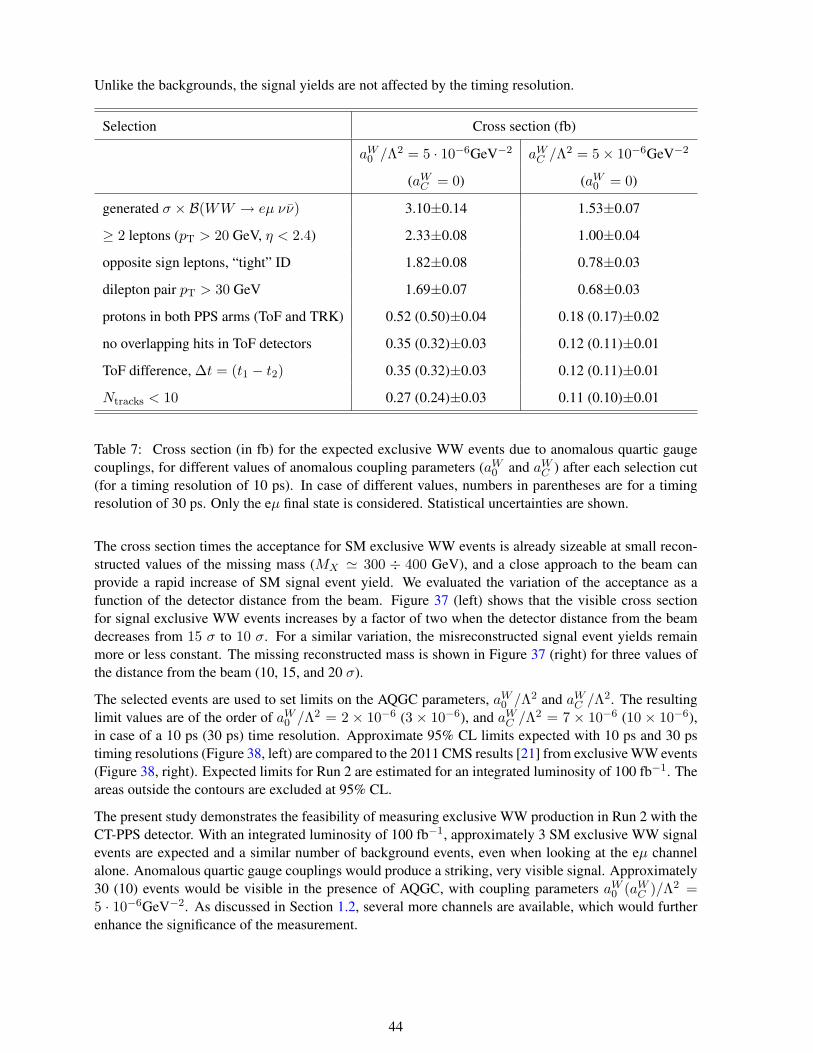
Unlike the backgrounds, the signal yields are not affected by the timing resolution.

Selection Cross section (fb)

aW0 /Λ2 = 5 · 10−6GeV−2 aW

C /Λ2 = 5× 10−6GeV−2

(aWC = 0) (aW

0 = 0)

generated σ × B(WW → eµ νν) 3.10±0.14 1.53±0.07

≥ 2 leptons (pT > 20 GeV, η < 2.4) 2.33±0.08 1.00±0.04

opposite sign leptons, “tight” ID 1.82±0.08 0.78±0.03

dilepton pair pT > 30 GeV 1.69±0.07 0.68±0.03

protons in both PPS arms (ToF and TRK) 0.52 (0.50)±0.04 0.18 (0.17)±0.02

no overlapping hits in ToF detectors 0.35 (0.32)±0.03 0.12 (0.11)±0.01

ToF difference, ∆t = (t1 − t2) 0.35 (0.32)±0.03 0.12 (0.11)±0.01

Ntracks < 10 0.27 (0.24)±0.03 0.11 (0.10)±0.01

Table 7: Cross section (in fb) for the expected exclusive WW events due to anomalous quartic gaugecouplings, for different values of anomalous coupling parameters (aW

0 and aWC ) after each selection cut

(for a timing resolution of 10 ps). In case of different values, numbers in parentheses are for a timingresolution of 30 ps. Only the eµ final state is considered. Statistical uncertainties are shown.

The cross section times the acceptance for SM exclusive WW events is already sizeable at small recon-structed values of the missing mass (MX ' 300 ÷ 400 GeV), and a close approach to the beam canprovide a rapid increase of SM signal event yield. We evaluated the variation of the acceptance as afunction of the detector distance from the beam. Figure 37 (left) shows that the visible cross sectionfor signal exclusive WW events increases by a factor of two when the detector distance from the beamdecreases from 15 σ to 10 σ. For a similar variation, the misreconstructed signal event yields remainmore or less constant. The missing reconstructed mass is shown in Figure 37 (right) for three values ofthe distance from the beam (10, 15, and 20 σ).

The selected events are used to set limits on the AQGC parameters, aW0 /Λ2 and aW

C /Λ2. The resultinglimit values are of the order of aW

0 /Λ2 = 2 × 10−6 (3 × 10−6), and aWC /Λ2 = 7 × 10−6 (10 × 10−6),

in case of a 10 ps (30 ps) time resolution. Approximate 95% CL limits expected with 10 ps and 30 pstiming resolutions (Figure 38, left) are compared to the 2011 CMS results [21] from exclusive WW events(Figure 38, right). Expected limits for Run 2 are estimated for an integrated luminosity of 100 fb−1. Theareas outside the contours are excluded at 95% CL.

The present study demonstrates the feasibility of measuring exclusive WW production in Run 2 with theCT-PPS detector. With an integrated luminosity of 100 fb−1, approximately 3 SM exclusive WW signalevents are expected and a similar number of background events, even when looking at the eµ channelalone. Anomalous quartic gauge couplings would produce a striking, very visible signal. Approximately30 (10) events would be visible in the presence of AQGC, with coupling parameters aW

0 (aWC )/Λ2 =

5 · 10−6GeV−2. As discussed in Section 1.2, several more channels are available, which would furtherenhance the significance of the measurement.

44

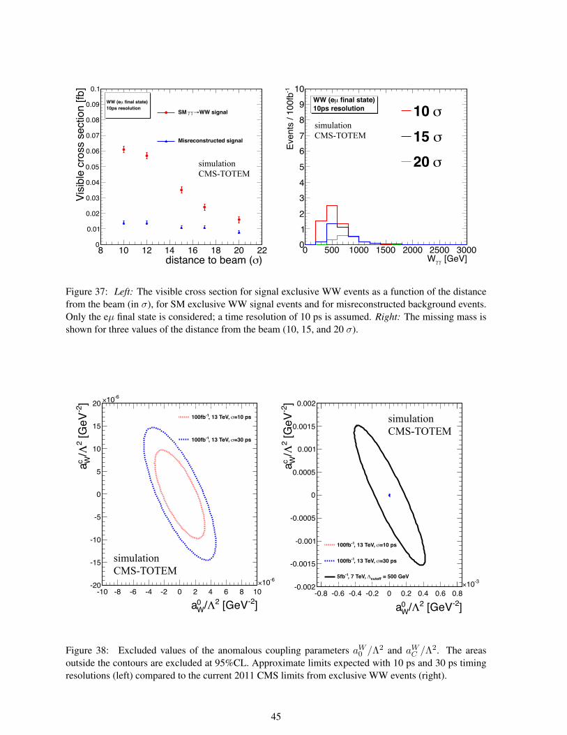
)σdistance to beam (8 10 12 14 16 18 20 22

Visi

ble

cros

s se

ctio

n [fb

]

0

0.01

0.02

0.03

0.04

0.05

0.06

0.07

0.08

0.09

0.1

WW signal→γγSM

Misreconstructed signal

10ps resolution final state)µWW (e


[GeV]γγW0 500 1000 1500 2000 2500 3000

-1Ev

ents

/ 10

0fb

0123456789

10

σ10 σ15 σ20

10ps resolution final state)µWW (e


Figure 37: Left: The visible cross section for signal exclusive WW events as a function of the distancefrom the beam (in σ), for SM exclusive WW signal events and for misreconstructed background events.Only the eµ final state is considered; a time resolution of 10 ps is assumed. Right: The missing mass isshown for three values of the distance from the beam (10, 15, and 20 σ).

]-2 [GeV2Λ/W0a

-10 -8 -6 -4 -2 0 2 4 6 8 10-610×

]-2

[GeV

2Λ/

Wc a

-20

-15

-10

-5

0

5

10

15

20-610×

=10 psσ, 13 TeV, -1100fb

=30 psσ, 13 TeV, -1100fb


]-2 [GeV2Λ/W0a

-0.8 -0.6 -0.4 -0.2 0 0.2 0.4 0.6 0.8-310×

]-2

[GeV

2Λ/

Wc a

-0.002

-0.0015

-0.001

-0.0005

0

0.0005

0.001

0.0015

0.002

=10 psσ, 13 TeV, -1100fb

=30 psσ, 13 TeV, -1100fb

= 500 GeVcutoffΛ, 7 TeV, -15fb


Figure 38: Excluded values of the anomalous coupling parameters aW0 /Λ2 and aW

C /Λ2. The areasoutside the contours are excluded at 95%CL. Approximate limits expected with 10 ps and 30 ps timingresolutions (left) compared to the current 2011 CMS limits from exclusive WW events (right).

45

References

[1] G. Antchev et al. [TOTEM Collaboration], “LHC optics measurement with proton tracks detectedby the roman pots of the TOTEM experiment”, arXiv:1406.0546 [physics.acc-ph].

[2] J. Favereau de Jeneret, X. Rouby, K. Piotrzkowski, JINST 2 (2007) P09005; arXiv:0707.1198.

[3] A. Latina and L. Deniau, “Evolution of MAD-X in the Framework of LHC Upgrade Studies”, Conf.Proc. C 1205201, 304 (2012).

[4] M. Benedikt, P. Collier, V. Mertens, J. Poole and K. Schindl, “LHC Design Report. 3. The LHCinjector chain”, CERN-2004-003-V-3.

[5] J. Monk and A. Pilkington, “ExHuME: A Monte Carlo event generator for exclusive diffraction”,Comput. Phys. Commun. 175, 232 (2006) [hep-ph/0502077].

[6] T. Sjostrand, S. Mrenna and P. Z. Skands, “PYTHIA 6.4 Physics and Manual”, JHEP 05 (2006)026 [hep-ph/0603175].

[7] M. Boonekamp, A. Dechambre, V. Juranek, O. Kepka, M. Rangel, C. Royon and R. Staszewski,“FPMC: A Generator for forward physics”, arXiv:1102.2531 [hep-ph].

[8] G. Corcella, I. G. Knowles, G. Marchesini, S. Moretti, K. Odagiri, P. Richardson, M. H. Seymourand B. R. Webber, “HERWIG 6.5 release note”, hep-ph/0210213.

[9] T. Sjostrand, S. Mrenna and P. Z. Skands, “A Brief Introduction to PYTHIA 8.1”, Comput. Phys.Commun. 178 (2008) 852 [arXiv:0710.3820 [hep-ph]].

[10] J. Allison, K. Amako, J. Apostolakis, H. Araujo, P. A. Dubois, M. Asai, G. Barrand and R. Capraet al., “Geant4 developments and applications”, IEEE Trans. Nucl. Sci. 53 (2006) 270.

[11] H. Niewiadomski, “Reconstruction of protons in the TOTEM roman pot detectors at the LHC”,PhD thesis, CERN-THESIS-2008-080.

[12] M. Berretti, “Performance studies of the Roman Pot timing detectors in the forward region of theIP5 at LHC”, TOTEM-NOTE 2014-001

[13] J. Kaspar, “Elastic scattering at the LHC”, Ph.D. thesis, CERN-THESIS-2011-214.

[14] T. Aaltonen et al. [CDF Collaboration], “Diffractive dijet production in pp collisions at√s =

1.96 TeV”, Phys. Rev. D 86, 032009 (2012) [arXiv:0712.0604 [hep-ex]].

[15] T. Aaltonen et al. [CDF Collaboration], “Observation of exclusive dijet production at the FermilabTevatron pp Collider”, Phys. Rev. D 77, 052004 (2008), [arXiv:0712.0604 [hep-ex]].

[16] S. Chatrchyan et al. [CMS Collaboration], “Observation of a diffractive contribution to dijetproduction in proton-proton collisions at

√s = 7 TeV”, Phys. Rev. D 87, 012006 (2013),

[arXiv:1209.1805 [hep-ex]].

[17] M. Cacciari, G. P. Salam and G. Soyez, “The anti-kT jet clustering algorithm”, JHEP 0804 (2008)063 [arXiv:0802.1189 [hep-ph]].

[18] M. Trzebinski, “Study of QCD and Diffraction with the ATLAS detector at the LHC”, CERN-THESIS-2013-166.

[19] T. Pierzchala and K. Piotrzkowski, “Sensitivity to anomalous quartic gauge couplings in photon-photon interactions at the LHC”, Nucl. Phys. Proc. Suppl. 179-180, 257 (2008) [arXiv:0807.1121[hep-ph]].

46

[20] E. Chapon, C. Royon and O. Kepka, “Anomalous quartic WWγγ, ZZγγ, and trilinear WWγ cou-plings in two-photon processes at high luminosity at the LHC”, Phys. Rev. D 81, 074003 (2010)[arXiv:0912.5161 [hep-ph]].

[21] S. Chatrchyan et al. [CMS Collaboration], “Study of exclusive two-photon production of W+W−

in pp collisions at√s = 7 TeV and constraints on anomalous quartic gauge couplings”, JHEP

1307, 116 (2013) [arXiv:1305.5596 [hep-ex]].

47

3 Beam Pockets

3.1 The Roman Pot system and collimators in the 200 m region of IP5

Within the combined TOTEM consolidation [1, 2] & CT-PPS project the beam line in the LHC regionof ±200 m from IP5 combines the RP220 m stations (220-Near, 220-Far), the relocated 147 m stations(210-Near, 210-Far) and new RP timing stations downstream of the 220 near station (Figure 39). The210 m far units are rotated by 8 degrees with respect to the beam line to improve the multitrack res-olution (Figure 41). During LS1 the vertical 210 m RPs and all 220 m RPs have been equipped withnew ferrites (TT2) and improved mechanical support frames to compensate for thermal expansion andallowing mechanical stress release. Within the TOTEM R&D project a cylindrical RP has been newlydesigned to house timing detectors and was optimized in view of material budget and RF interaction withthe LHC beam. Furthermore, the horizontal RP210 have been optimized to reduce the RF interactionwith LHC by keeping the original box design of the standard TOTEM RP. Furthermore TCL4 and TCL6collimators have been installed [3] in front of the Q4 and Q6 quadrupoles, respectively. Figure 40 showsthe beamline in Sector 4-5 with the RPs installed.

Figure 39: The layout of the beam line in the 200 m region after LS1

3.2 New Roman Pots for timing detectors

The new RPs installed between the existing units 220-N and 220-F are intended to host timing detectors.Hence their design was subject to the following main requirements:

1. Among several potential detector technologies for the timing measurements (see Section 5.1),

48

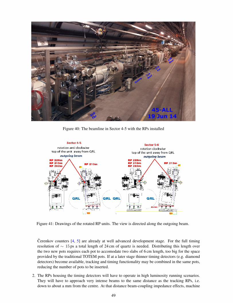
Figure 40: The beamline in Sector 4-5 with the RPs installed

Figure 41: Drawings of the rotated RP units. The view is directed along the outgoing beam.

Cerenkov counters [4, 5] are already at well advanced development stage. For the full timingresolution of ∼ 15 ps a total length of 24 cm of quartz is needed. Distributing this length overthe two new pots requires each pot to accomodate two slabs of 6 cm length, too big for the spaceprovided by the traditional TOTEM pots. If at a later stage thinner timing detectors (e.g. diamonddetectors) become available, tracking and timing functionality may be combined in the same pots,reducing the number of pots to be inserted.

2. The RPs housing the timing detectors will have to operate in high luminosity running scenarios.They will have to approach very intense beams to the same distance as the tracking RPs, i.e.down to about a mm from the centre. At that distance beam-coupling impedance effects, machine

49

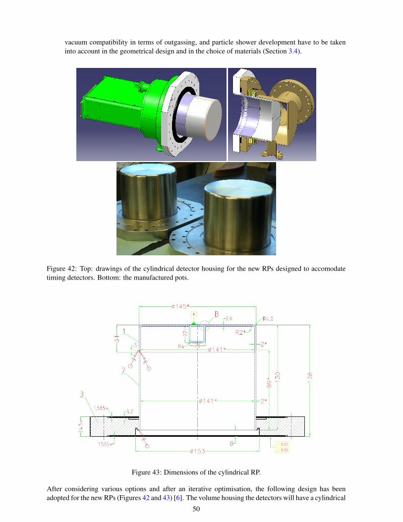
vacuum compatibility in terms of outgassing, and particle shower development have to be takeninto account in the geometrical design and in the choice of materials (Section 3.4).

Figure 42: Top: drawings of the cylindrical detector housing for the new RPs designed to accomodatetiming detectors. Bottom: the manufactured pots.

Figure 43: Dimensions of the cylindrical RP.

After considering various options and after an iterative optimisation, the following design has beenadopted for the new RPs (Figures 42 and 43) [6]. The volume housing the detectors will have a cylindrical

50

rather than rectangular box shape. This choice provides the necessary space for all potential technologiesof timing detectors and at the same time reduces the beam coupling impedance by minimising resonantcavities. The ferrite in this design will be integrated in the (stationary) flange rather than mounted on themoving detector housing. It will have a ring geometry (inner diameter = 150 mm, radial width = 15 mm,thickness = 5 mm). Furthermore, all vacuum-side surfaces of the RP stations are foreseen to receive a2µm thick Non-Evaporative Getter (NEG) coating.

3.2.1 The mechanical tests of new Roman Pot cylinders

The new cylindrical Roman Pots with the thin window of 300 µm thickness have been produced (seeFigure 42) in a collaboration of CERN with industries. After the production of the first prototype infall 2013 a series of test have been performed at CERN in collaboration with different support groups,to approve the compatibility of this new RP design with the LHC requirements. The deflection of thethin window was measured as function of the applied air overpressure simulating the possible pressuredifference seen by the RP when the LHC beam tube is under vacuum and the inner side of the RP isunder atmospheric pressure. Such pressure difference will arrive during the installation of the detectorcomponents or a failure of the vacuum system and a leak of the feedthrough integrated in the flangeseparating the atmosphere from the inner side of the RP [7]. Furthermore the He transmission wasmeasured in a special setup and the compatibility of this design with the LHC leak rate requirements wasshown [8].

3.3 The RF Shield for the box-shaped horizontal Roman Pots

Given that the existing horizontal pots housing tracking detectors will have to cope with the same highluminosity conditions as the new timing RPs, some adaptations will be made:

• To reach the same impedance reduction as for the new cylindrical pots (see Section 3.4.2), therectangular detector boxes will be successively equipped with 1 mm thick cylindrical copper RFshields (Figure 44). Holes in the shield allow for the gas flow necessary to establish a vacuumequilibrium inside and outside the shield. The number and dimensions of these holes have beendefined in cooperation with the LHC vacuum group: In the lateral, cylindrical wall there are 3rows of 15 circular holes each with a diameter of 1 cm; the wall facing the beam has 8 slits of3 × 12mm2 with rounded corners (2 mm radius). The shield is retracted by 30 mm from the boxwindow facing the beam, in order not to intercept any signal protons with the shield material. Inthe first step, during LS1, the horizontal pots of the RP210 station will receive the RF shields, inorder to gain experience without touching the RP220 station.

• The horizontal RP210 stations will be equipped with new vacuum bellows and modified flangesthat allow to integrate the same ferrite geometry as used in the new RPs. The ferrites of the verticalRPs of the RP210 stations will be exchanged with the new TT2 material as in the RP220 stations.

3.4 Interaction with the beam environment

3.4.1 Experience from 2012

In October and November 2012 several test insertions of the RPs in normal high-luminosity fills at√s = 8 TeV with β∗ = 0.6 m were performed. While the vertical pots had no problems to reach the

target distance of 12 σ from the beam centre, the horizontal pots encountered a very intense collisiondebris halo, and repeatedly the beam was dumped by showers hitting the Beam Loss Monitors at a pot

51

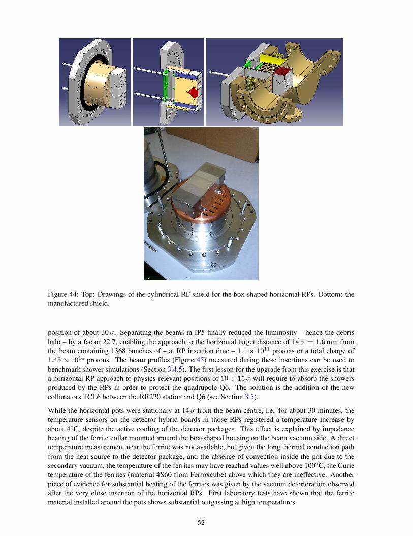
Figure 44: Top: Drawings of the cylindrical RF shield for the box-shaped horizontal RPs. Bottom: themanufactured shield.

position of about 30σ. Separating the beams in IP5 finally reduced the luminosity – hence the debrishalo – by a factor 22.7, enabling the approach to the horizontal target distance of 14σ = 1.6 mm fromthe beam containing 1368 bunches of – at RP insertion time – 1.1 × 1011 protons or a total charge of1.45 × 1014 protons. The beam profiles (Figure 45) measured during these insertions can be used tobenchmark shower simulations (Section 3.4.5). The first lesson for the upgrade from this exercise is thata horizontal RP approach to physics-relevant positions of 10 ÷ 15σ will require to absorb the showersproduced by the RPs in order to protect the quadrupole Q6. The solution is the addition of the newcollimators TCL6 between the RR220 station and Q6 (see Section 3.5).

While the horizontal pots were stationary at 14σ from the beam centre, i.e. for about 30 minutes, thetemperature sensors on the detector hybrid boards in those RPs registered a temperature increase byabout 4C, despite the active cooling of the detector packages. This effect is explained by impedanceheating of the ferrite collar mounted around the box-shaped housing on the beam vacuum side. A directtemperature measurement near the ferrite was not available, but given the long thermal conduction pathfrom the heat source to the detector package, and the absence of convection inside the pot due to thesecondary vacuum, the temperature of the ferrites may have reached values well above 100C, the Curietemperature of the ferrites (material 4S60 from Ferroxcube) above which they are ineffective. Anotherpiece of evidence for substantial heating of the ferrites was given by the vacuum deterioration observedafter the very close insertion of the horizontal RPs. First laboratory tests have shown that the ferritematerial installed around the pots shows substantial outgassing at high temperatures.

52

Figure 45: Left: vertical beam profile measured via the trigger rates in the detectors of the top and bottompots of Sector 56,220-N. Right: horizontal beam profile measured in Sector 45,220-N; the luminosity re-duction by beam separation has been corrected for. The reconstructed curve is the result of a convolutionfit discussed in [9].

Triggered by the problems and observations described above, a programme of simulations, extendedlaboratory tests, and design optimisations was defined; it is discussed in the following section.

3.4.2 Impedance

As mentioned in the previous section, during a RP insertion to 1.6 mm from a high-intensity beam (1368bunches of 1.1× 1011 protons) a temperature increase was observed on the detector hybrid boards. Thiseffect can probably be attributed to impedance heating. It is hypothesised that the 4S60 ferrite mountedaround the RP box reached a temperature above 100C, the Curie temperature, which resulted in the lossof ferrite effectiveness and hence even stronger heating by the now non-damped cavity resonance near550 MHz [10]. Note, however, that no other impedance effects were observed, in particular, no beaminstabilities.

The aim of the work presented here [11] is the optimisation of the RP design to minimise the beam-coupling impedance, in particular at very close distances to the beam, in view of more regular andextended RP insertions in the future.

The impedance seen by a beam of particles has contributions from the shape of the vacuum chamber(geometrical impedance) and from the finite conductivity of the material used for its construction. Theremainder of this section focusses on the dominant geometrical contribution of three RP designs: thestandard box-shaped RP, the new cylindrical RP, and the improved box-shaped RP with shield (intro-duced in Section 3.3).

The study was performed by simulating the passage of a charge distribution (source charge) through acavity, in this case through a RP, and computing the wake field felt by a longitudinally or transverselydisplaced second charge (test charge). The potential felt by the test charge is then used to compute thelongitudinal or transverse impedance using Fourier Transforms.

Three impedance effects have to be addressed:

• Beam-induced heating, i.e. the transfer of power from the beam to the lossy wall of a cavity,is determined by the frequency-dependent real part of the longitudinal impedance in conjunction

53

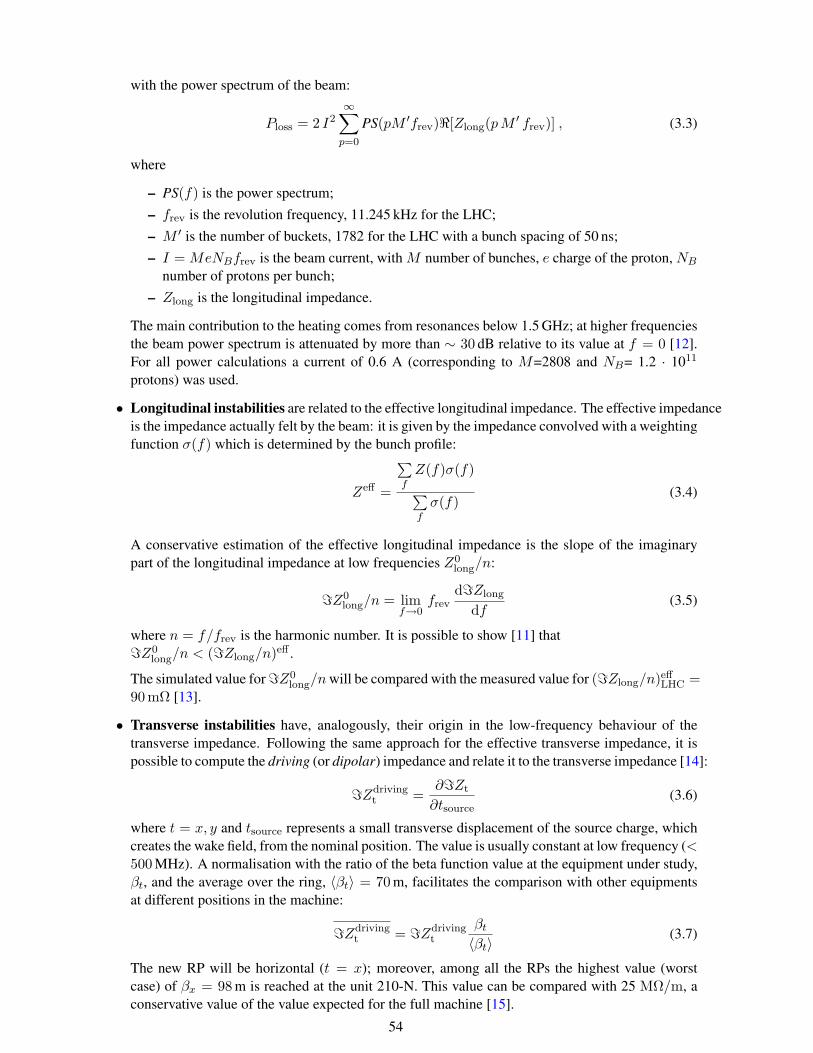
with the power spectrum of the beam:

Ploss = 2 I2∞∑

p=0

PS(pM ′frev)<[Zlong(pM ′ frev)] , (3.3)

where

– PS(f) is the power spectrum;– frev is the revolution frequency, 11.245 kHz for the LHC;– M ′ is the number of buckets, 1782 for the LHC with a bunch spacing of 50 ns;– I = MeNBfrev is the beam current, with M number of bunches, e charge of the proton, NB

number of protons per bunch;– Zlong is the longitudinal impedance.

The main contribution to the heating comes from resonances below 1.5 GHz; at higher frequenciesthe beam power spectrum is attenuated by more than ∼ 30 dB relative to its value at f = 0 [12].For all power calculations a current of 0.6 A (corresponding to M=2808 and NB= 1.2 · 1011

protons) was used.

• Longitudinal instabilities are related to the effective longitudinal impedance. The effective impedanceis the impedance actually felt by the beam: it is given by the impedance convolved with a weightingfunction σ(f) which is determined by the bunch profile:

Zeff =

∑f

Z(f)σ(f)∑f

σ(f)(3.4)

A conservative estimation of the effective longitudinal impedance is the slope of the imaginarypart of the longitudinal impedance at low frequencies Z0

long/n:

=Z0long/n = lim

f→0frev

d=Zlong

df(3.5)

where n = f/frev is the harmonic number. It is possible to show [11] that=Z0

long/n < (=Zlong/n)eff .

The simulated value for=Z0long/nwill be compared with the measured value for (=Zlong/n)effLHC =

90 mΩ [13].

• Transverse instabilities have, analogously, their origin in the low-frequency behaviour of thetransverse impedance. Following the same approach for the effective transverse impedance, it ispossible to compute the driving (or dipolar) impedance and relate it to the transverse impedance [14]:

=Zdrivingt =

∂=Zt

∂tsource(3.6)

where t = x, y and tsource represents a small transverse displacement of the source charge, whichcreates the wake field, from the nominal position. The value is usually constant at low frequency (<500 MHz). A normalisation with the ratio of the beta function value at the equipment under study,βt, and the average over the ring, 〈βt〉 = 70 m, facilitates the comparison with other equipmentsat different positions in the machine:

=Zdrivingt = =Zdriving

t

βt

〈βt〉(3.7)

The new RP will be horizontal (t = x); moreover, among all the RPs the highest value (worstcase) of βx = 98 m is reached at the unit 210-N. This value can be compared with 25 MΩ/m, aconservative value of the value expected for the full machine [15].

54

For the new cylindrical pots, simulation results indicate that no low frequency resonances (< 1.4 GHz)are present if the gap between the detector housing and the flange is completely closed, which of courseprevents any RP movement. Mechanical constraints require at least 2.5 mm gap between the housingand the flange. With this gap a resonance at 470 MHz appears, as shown in Figure 46; its impedance,however, is smaller than for the standard box-shaped RP. The position and the dimensions of the ferrite

Figure 46: Simulated <[Zlong] of the cylindrical RP without ferrite. The resonance at 470 MHz is dueto the cavity between the flange and the detector housing. The darkened part of the graph has negligibleimpact on the heating due to the strongly attenuated LHC power spectrum at such high frequencies.

has been optimised through various iterations considering also vacuum and mechanical construction.The final design consists of a ferrite ring (inner diameter = 150 mm, radial width = 15 mm, thickness =5 mm) integrated into the flange, as far as possible from the beam (Figure 47). This design is feasibleand can be easily integrated in the existing design.

Figure 47: Detail of the geometrical model used in the impedance simulations. It shows the new ferritering to be integrated in the flanges of the cylindrical pots and of the improved pots with shields.

Figure 48 shows the real and imaginary parts of the longitudinal impedances of the three RP designswith ferrites. In all cases, the 470 MHz resonance is damped and smeared beyond recognition. Atlow frequencies, the cylindrical and shielded RPs have a smaller <[Zlong] than the standard RP. This isalso reflected by the reduced heating for the new designs (Figure 49). Figure 50 shows the effectivelongitudinal impedance as a function of the RP distance from the beam. Also here, the new designs haveled to a significant reduction.

These results are numerically summarised in Table 8.

55

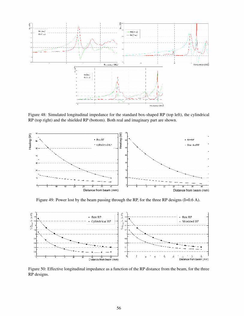
Figure 48: Simulated longitudinal impedance for the standard box-shaped RP (top left), the cylindricalRP (top right) and the shielded RP (bottom). Both real and imaginary part are shown.

Figure 49: Power lost by the beam passing through the RP, for the three RP designs (I=0.6 A).

Figure 50: Effective longitudinal impedance as a function of the RP distance from the beam, for the threeRP designs.

56

Distance fromthebeam [mm]

=Z0longn

[mΩ]fraction of(=Zlong

n)effLHC

(90 mΩ)

=Zdrivingtrans

[MΩ/m]fraction of=(Zx)

effLHC

(25 MΩ/m)

Heating[W]I=0.6 A

Box RP

1 1.7 < 1.9 % 0.15 < 0.6 % 62

5 1.3 < 1.4 % 52

40 (garage) 0.41 < 0.45 % 10

Cylindrical RP

1 1.1 < 1.2 % 0.11 < 0.5 % 13

5 0.73 < 0.81 % 11

40 (garage) 0.18 < 0.20 % 4

ShieldedRP

1 1.2 < 1.3 % 0.2 < 0.8 % 10

40 (garage) 0.30 < 0.33 % 2

Table 8: Main results of the simulation of the present box RP (Box RP), the cylindrical RP (CylindricalRP), and the Box RP with Shield. Longitudinal and transverse impedances are compared with the totalvalues estimated for the present LHC effective impedances.

3.4.3 The RF test in the lab

The new cylindrical RP and the RF shield in combination with ferrites were developed to reduce the RFinteraction with the LHC beam. Prior the serial production of components a new RP cross with flangesand bellow was manufactured. The prototype of the cylindrical RP and the RF shield in combination withthe box-shaped RP have been integrated in this new RP cross for RF measurements. In February 2014measurements were performed by TOTEM and the LHC impedance group in the TIF lab of CERN. Indetailed measurements with and without the new ferrites and at different insertion positions of the RP, theRF characteristics of this new geometry could be determined and good agreement with the predictions,based on simulations could be found [16].

3.4.4 Vacuum

The vacuum degradations observed in 2012 after very close horizontal RP insertions to high-intensitybeams triggered the following consolidation activities for improving the vacuum compatibility of the RPsystem:

• Ferrite material improvements:The 4S60 ferrites used in the RP system before LS1 are now (but not in 2006) known to showhigh outgassing rates unless they are baked out at 1000C [17]. In the TOTEM RPs these ferriteswere installed as received from the manufacturer and then baked out in situ at about 200C like allother beam-pipe components, which turned out not to be sufficient. Since the 4S60 ferrites have inaddition a low Curie temperature of only 100C, alternative ferrite materials are being investigatedinstead of only baking out the 4S60 material at 1000C. The material used for the TOTEM RPs isTT2-111R from TransTech with a Curie temperature of 375C and an acceptable outgassing afterbake-out at 1000C [18]. An alternative material for possible future use is 4E2 (Ferroxcube) witha Curie temperature of about 400C; its outgassing behaviour remains to be tested.

• The new geometrical ferrite configuration reduces the ferrite surfaces exposed to the vacuum byan order of magnitude from 220 cm2 per standard RP to 23 cm2 per cylindrical RP.

• All components exposed to the primary beam vacuum have been proposed by the vacuum groupto be coated with NEG, as far as technically possible.

57

3.4.5 Generation of particle showers

To assess the generation of particle showers by RPs interacting with the intense debris halo (see 2012experience discussed in Section 3.4.1), Geant4 simulations implementing detailed models of the rectan-gular and the new cylindrical RPs have been carried out [9].

The first goal of the study was to identify the contributions from the different structural elements of aRP to the shower creation. For this purpose, 7 TeV protons with a delta-function profile distribution, i.e.zero width and zero angular spread, were shot parallel to the beam onto three elements of a pot:

• through the beam-facing window, 50µm from the outer surface;

• through the front window, the detector planes and the rear window, 2 cm from the outer surface ofthe beam-facing window;

• through the body wall of the pot, 6 cm from the outer surface of the beam-facing window.

This was performed for the standard rectangular pot geometry and for the new cylindrical one (see Table 9for some key dimensions). For each case a sample of 2000 protons was processed. Figure 51 shows theresulting angular distributions of the secondary particles produced in the RP material.

RP Element Standard Pot Cylindrical Pot

Beam-facing window length along beam 54 mm 145 mm

Beam-facing window thickness 0.15 mm 0.3 mm

Front / back window 0.5 mm 0.3 mm

Body wall thickness 2 mm 3 mm

Table 9: Comparison of the standard and cylindrical RP elements most relevant for the material budgetand hence for shower production.

As expected, the number of secondary particles is mostly determined by the amount of material traversed.The key observations are:

• In both RP designs, the bottom foil produces by far the highest number of secondary particles,followed by the thick body walls with 2 to 3.5 orders of magnitude lower rates. The orthogonallytraversed thin front and back windows produce the lowest numbers of secondaries.

• The bottom foil of the cylindrical pots produces more than 10 times more secondaries than themuch shorter foil of the standard pots. In the other elements the shower production is similar inthe two designs.

• The showers from the bottom foil of the cylindrical pot are 3 times wider than the ones from thestandard pots: 99% contained in 0.6 rad = 34 rather than in 0.2 rad = 11.

• The two projections, horizontal and vertical, are almost identical.

The second part of the study addressed the shower production by particles distributed according to therate density profile dN/dt dx dy deconvoluted [9] from the trigger rate profile measured in November2012 (Figure 45). This gives a picture of the total shower distribution, in contrast to the first study thatfocused on the delta-response of the individual components. Figure 52 shows the simulated secondaryparticle distribution in a scoring plane 6 m downstream of a standard horizontal RP inserted to 2 mm from

58

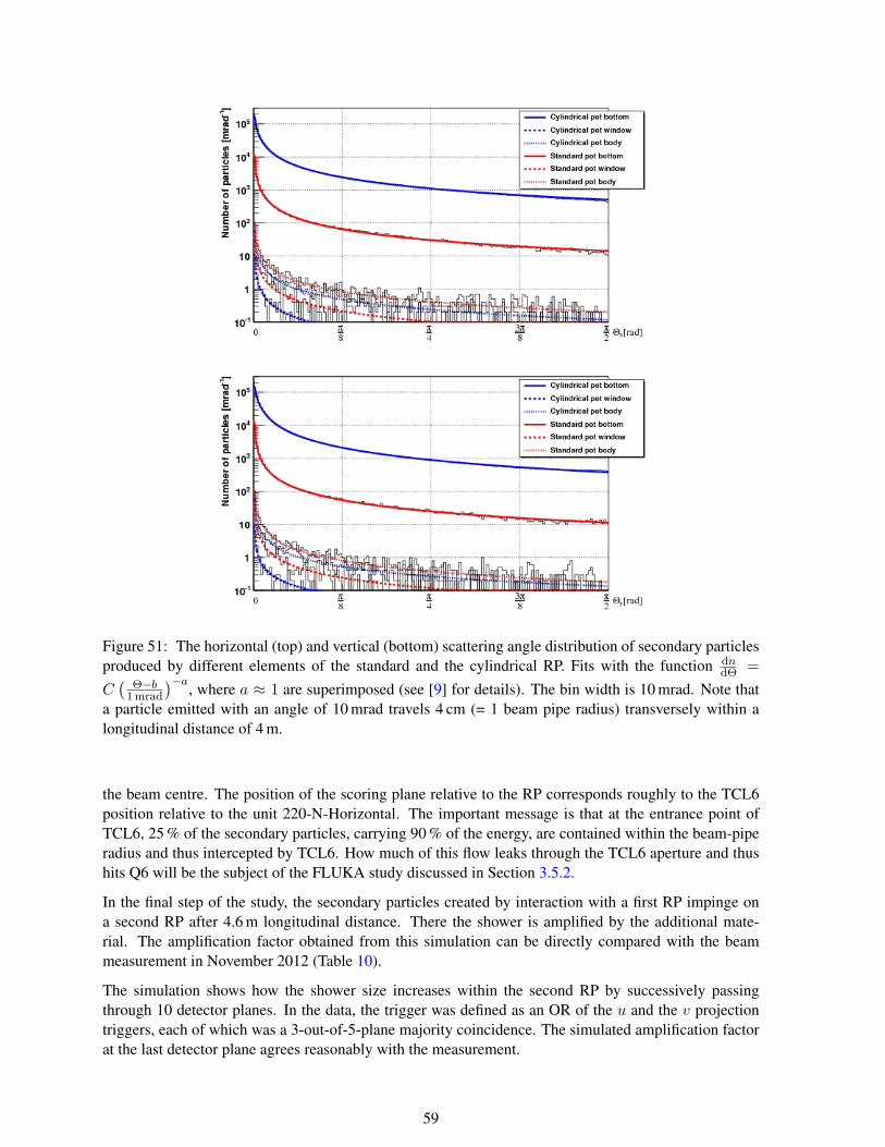
Figure 51: The horizontal (top) and vertical (bottom) scattering angle distribution of secondary particlesproduced by different elements of the standard and the cylindrical RP. Fits with the function dn

dΘ =C

(Θ−b

1mrad

)−a, where a ≈ 1 are superimposed (see [9] for details). The bin width is 10 mrad. Note that

a particle emitted with an angle of 10 mrad travels 4 cm (= 1 beam pipe radius) transversely within alongitudinal distance of 4 m.

the beam centre. The position of the scoring plane relative to the RP corresponds roughly to the TCL6position relative to the unit 220-N-Horizontal. The important message is that at the entrance point ofTCL6, 25 % of the secondary particles, carrying 90 % of the energy, are contained within the beam-piperadius and thus intercepted by TCL6. How much of this flow leaks through the TCL6 aperture and thushits Q6 will be the subject of the FLUKA study discussed in Section 3.5.2.

In the final step of the study, the secondary particles created by interaction with a first RP impinge ona second RP after 4.6 m longitudinal distance. There the shower is amplified by the additional mate-rial. The amplification factor obtained from this simulation can be directly compared with the beammeasurement in November 2012 (Table 10).

The simulation shows how the shower size increases within the second RP by successively passingthrough 10 detector planes. In the data, the trigger was defined as an OR of the u and the v projectiontriggers, each of which was a 3-out-of-5-plane majority coincidence. The simulated amplification factorat the last detector plane agrees reasonably with the measurement.

59

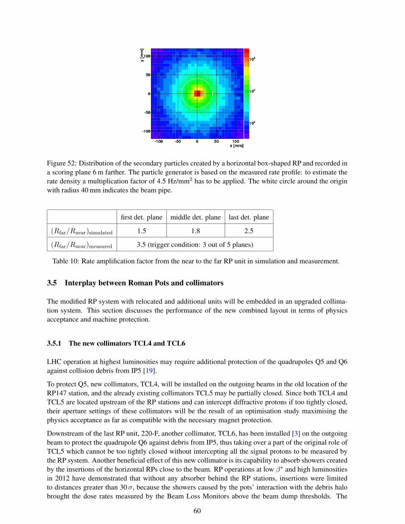
Figure 52: Distribution of the secondary particles created by a horizontal box-shaped RP and recorded ina scoring plane 6 m farther. The particle generator is based on the measured rate profile: to estimate therate density a multiplication factor of 4.5 Hz/mm2 has to be applied. The white circle around the originwith radius 40 mm indicates the beam pipe.

first det. plane middle det. plane last det. plane

(Rfar/Rnear)simulated 1.5 1.8 2.5

(Rfar/Rnear)measured 3.5 (trigger condition: 3 out of 5 planes)

Table 10: Rate amplification factor from the near to the far RP unit in simulation and measurement.

3.5 Interplay between Roman Pots and collimators

The modified RP system with relocated and additional units will be embedded in an upgraded collima-tion system. This section discusses the performance of the new combined layout in terms of physicsacceptance and machine protection.

3.5.1 The new collimators TCL4 and TCL6

LHC operation at highest luminosities may require additional protection of the quadrupoles Q5 and Q6against collision debris from IP5 [19].

To protect Q5, new collimators, TCL4, will be installed on the outgoing beams in the old location of theRP147 station, and the already existing collimators TCL5 may be partially closed. Since both TCL4 andTCL5 are located upstream of the RP stations and can intercept diffractive protons if too tightly closed,their aperture settings of these collimators will be the result of an optimisation study maximising thephysics acceptance as far as compatible with the necessary magnet protection.

Downstream of the last RP unit, 220-F, another collimator, TCL6, has been installed [3] on the outgoingbeam to protect the quadrupole Q6 against debris from IP5, thus taking over a part of the original role ofTCL5 which cannot be too tightly closed without intercepting all the signal protons to be measured bythe RP system. Another beneficial effect of this new collimator is its capability to absorb showers createdby the insertions of the horizontal RPs close to the beam. RP operations at low β∗ and high luminositiesin 2012 have demonstrated that without any absorber behind the RP stations, insertions were limitedto distances greater than 30σ, because the showers caused by the pots’ interaction with the debris halobrought the dose rates measured by the Beam Loss Monitors above the beam dump thresholds. The

60

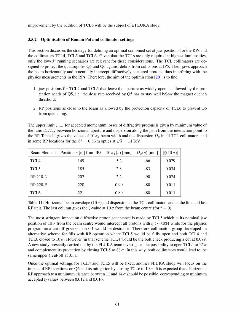
improvement by the addition of TCL6 will be the subject of a FLUKA study.

3.5.2 Optimisation of Roman Pot and collimator settings

This section discusses the strategy for defining an optimal combined set of jaw positions for the RPs andthe collimators TCL4, TCL5 and TCL6. Given that the TCLs are only required at highest luminosities,only the low-β∗ running scenarios are relevant for these considerations. The TCL collimators are de-signed to protect the quadrupoles Q5 and Q6 against debris from collisions at IP5. Their jaws approachthe beam horizontally and potentially intercept diffractively scattered protons, thus interfering with thephysics measurements in the RPs. Therefore, the aim of the optimisation [20] is to find

1. jaw positions for TCL4 and TCL5 that leave the aperture as widely open as allowed by the pro-tection needs of Q5, i.e. the dose rate received by Q5 has to stay well below the magnet quenchthreshold;

2. RP positions as close to the beam as allowed by the protection capacity of TCL6 to prevent Q6from quenching.

The upper limit ξmax for accepted momentum losses of diffractive protons is given by minimum value ofthe ratio dx/Dx between horizontal aperture and dispersion along the path from the interaction point tothe RP. Table 11 gives the values of 10σx beam width and the dispersion Dx in all TCL collimators andin some RP locations for the β∗ = 0.55 m optics at

√s = 14 TeV.

Beam Element Position s [m] from IP5 10σx(s) [mm] Dx(s) [mm] |ξ(10σ)|

TCL4 149 5.2 -66 0.079

TCL5 185 2.8 -83 0.034

RP 210-N 202 2.2 -90 0.024

RP 220-F 220 0.90 -80 0.011

TCL6 221 0.89 -80 0.011

Table 11: Horizontal beam envelope (10σ) and dispersion at the TCL collimators and at the first and lastRP unit. The last column gives the ξ-value at 10σ from the beam centre (for t = 0).

The most stringent impact on diffractive proton acceptance is made by TCL5 which at its nominal jawposition of 10σ from the beam centre would intercept all protons with ξ > 0.034 while for the physicsprogramme a cut-off greater than 0.1 would be desirable. Therefore collimation group developed analternative scheme for fills with RP operation where TCL5 would be fully open and both TCL4 andTCL6 closed to 10σ. However, in that scheme TCL4 would be the bottleneck producing a cut at 0.079.A new study presently carried out by the FLUKA team investigates the possibility to open TCL4 to 15σand complement its protection by closing TCL5 to 35σ. In this way, both collimators would lead to thesame upper ξ cut-off at 0.11.

Once the optimal settings for TCL4 and TCL5 will be fixed, another FLUKA study will focus on theimpact of RP insertions on Q6 and its mitigation by closing TCL6 to 10σ. It is expected that a horizontalRP approach to a minimum distance between 11 and 14σ should be possible, corresponding to minimumaccepted ξ-values between 0.012 and 0.016.

61

Figure 53: Left: Movable pipe with support table and detector box. The bellows, beam position monitors(square boxes), detector pocket, and drive motor are visible. Right: Detailed drawings of the movablepipe with support table and detector box. Shown are the (1) fixed support table; (2) guides; (3) movingsupport; (4) motor; (5) beam position monitor (fixed with respect to beam pipe); (6) bellows; (7) modifiedbeam-pipe with the indentation for the detectors; (8) detector box inside which the detectors are housed; itcan be made vacuum-tight if secondary vacuum is required; (9) beam position monitor (moving togetherwith the movable beam-pipe).

3.6 Movable Beam-Pipe

As a possible alternative to Roman Pots, we are pursuing development of a technique used originally bythe ZEUS collaboration at HERA [21], referred to as a movable beam-pipe or “Hamburg beam-pipe”.This consists of a large-diameter section of beam-pipe with a thin flat side wall, with integrated trackingand timing detectors inserted in a detector box attached to the pipe. The movable-pipe technique allowseasy access to the detectors, and maintains a fixed vacuum volume as the detectors are inserted into thevacuum. This results in low mechanical stress and consequently in a simple and robust design. In effect,the MBP is an instrumented collimator. Consequently, the LHC collimator control system and motordesign can be adopted with little modifications.

In routine operation, two positions will be used: the parking position and the operational position closeto the beam for data taking. The displacement between the two positions will be ∼25 mm. As discussedin Chapter 3, the distance of approach to the beam directly affects the low mass acceptance in exclusiveproduction. The MBP should therefore be designed to approach the beam as close as possible, ideally tobetter than 15σ.

Deploying one such station during the 2015-2016 year end technical stop will allow evaluation of theMBP solution during the exploratory phase of CT-PPS. A similar approach has been studied within theATLAS Forward Proton (AFP) project; the design described here incorporates several developmentsfrom AFP in view of allowing for a common design in the future.

Figure 53 (left) shows the layout of a full MBP station including one detector box and the support table.No secondary vacuum is assumed inside the detector box. However, secondary vacuum can be easilyimplemented in the current design if requested by the machine or desirable for detector operation. TheMBP station is fixed to the floor with independent supports, while the movable section is connected tothe standard beampipe by bellows. A single drive motor system is placed at the center. Two precisionbeam position monitors are required to measure the distance between the detectors and the beam center,one on the fixed pipe and one on the movable pipe. At each pocket there is a detector box, providingsecondary vacuum if necessary, with a lid for access, and feed-throughs. Figure 53 (right) illustrates theproposed layout of the full system in more detail.

62

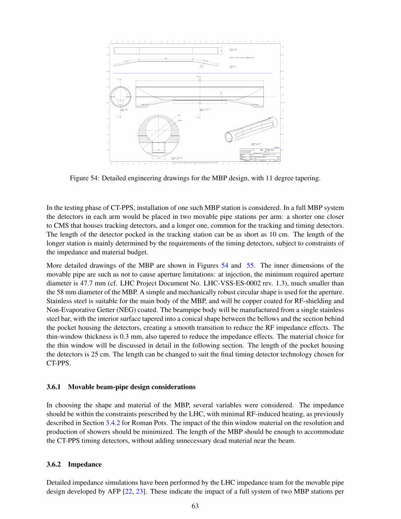
Figure 54: Detailed engineering drawings for the MBP design, with 11 degree tapering.

In the testing phase of CT-PPS, installation of one such MBP station is considered. In a full MBP systemthe detectors in each arm would be placed in two movable pipe stations per arm: a shorter one closerto CMS that houses tracking detectors, and a longer one, common for the tracking and timing detectors.The length of the detector pocked in the tracking station can be as short as 10 cm. The length of thelonger station is mainly determined by the requirements of the timing detectors, subject to constraints ofthe impedance and material budget.

More detailed drawings of the MBP are shown in Figures 54 and 55. The inner dimensions of themovable pipe are such as not to cause aperture limitations: at injection, the minimum required aperturediameter is 47.7 mm (cf. LHC Project Document No. LHC-VSS-ES-0002 rev. 1.3), much smaller thanthe 58 mm diameter of the MBP. A simple and mechanically robust circular shape is used for the aperture.Stainless steel is suitable for the main body of the MBP, and will be copper coated for RF-shielding andNon-Evaporative Getter (NEG) coated. The beampipe body will be manufactured from a single stainlesssteel bar, with the interior surface tapered into a conical shape between the bellows and the section behindthe pocket housing the detectors, creating a smooth transition to reduce the RF impedance effects. Thethin-window thickness is 0.3 mm, also tapered to reduce the impedance effects. The material choice forthe thin window will be discussed in detail in the following section. The length of the pocket housingthe detectors is 25 cm. The length can be changed to suit the final timing detector technology chosen forCT-PPS.

3.6.1 Movable beam-pipe design considerations

In choosing the shape and material of the MBP, several variables were considered. The impedanceshould be within the constraints prescribed by the LHC, with minimal RF-induced heating, as previouslydescribed in Section 3.4.2 for Roman Pots. The impact of the thin window material on the resolution andproduction of showers should be minimized. The length of the MBP should be enough to accommodatethe CT-PPS timing detectors, without adding unnecessary dead material near the beam.

3.6.2 Impedance

Detailed impedance simulations have been performed by the LHC impedance team for the movable pipedesign developed by AFP [22, 23]. These indicate the impact of a full system of two MBP stations per

63

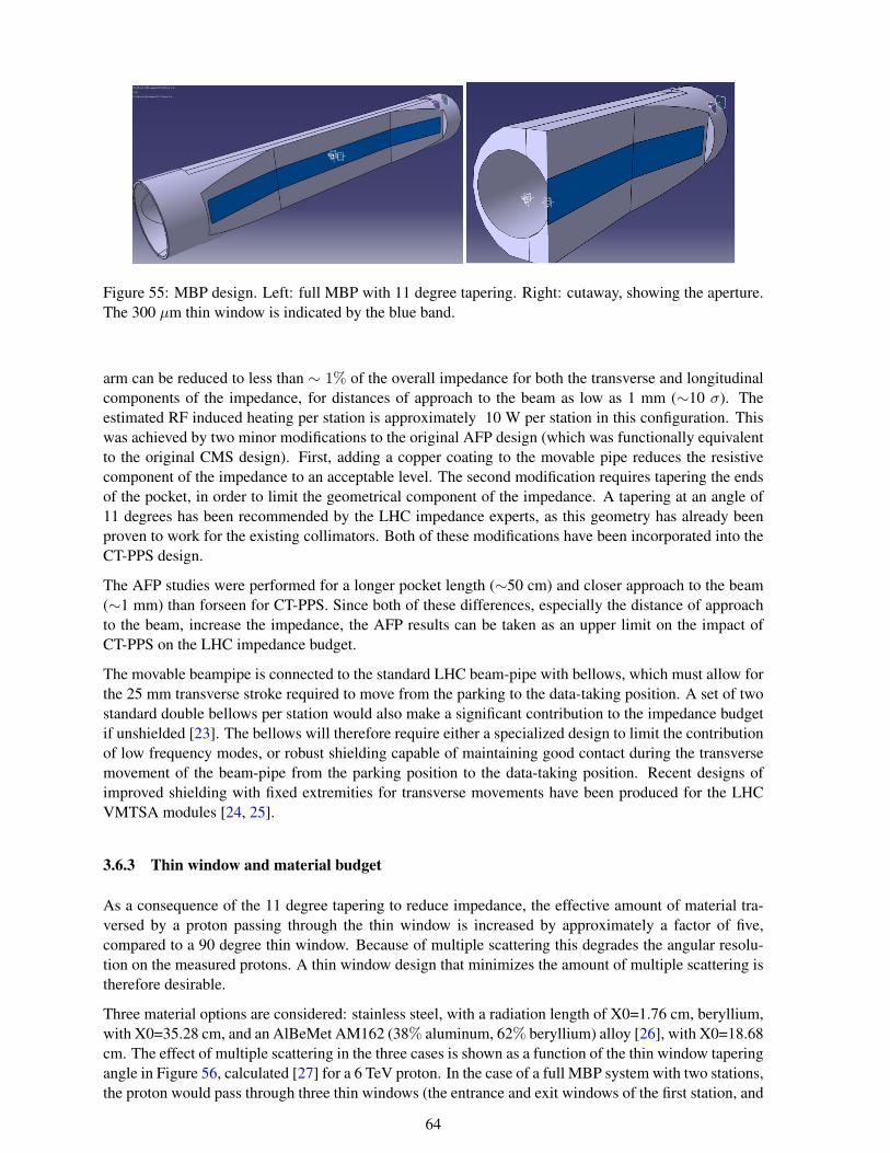
Figure 55: MBP design. Left: full MBP with 11 degree tapering. Right: cutaway, showing the aperture.The 300 µm thin window is indicated by the blue band.

arm can be reduced to less than ∼ 1% of the overall impedance for both the transverse and longitudinalcomponents of the impedance, for distances of approach to the beam as low as 1 mm (∼10 σ). Theestimated RF induced heating per station is approximately 10 W per station in this configuration. Thiswas achieved by two minor modifications to the original AFP design (which was functionally equivalentto the original CMS design). First, adding a copper coating to the movable pipe reduces the resistivecomponent of the impedance to an acceptable level. The second modification requires tapering the endsof the pocket, in order to limit the geometrical component of the impedance. A tapering at an angle of11 degrees has been recommended by the LHC impedance experts, as this geometry has already beenproven to work for the existing collimators. Both of these modifications have been incorporated into theCT-PPS design.

The AFP studies were performed for a longer pocket length (∼50 cm) and closer approach to the beam(∼1 mm) than forseen for CT-PPS. Since both of these differences, especially the distance of approachto the beam, increase the impedance, the AFP results can be taken as an upper limit on the impact ofCT-PPS on the LHC impedance budget.

The movable beampipe is connected to the standard LHC beam-pipe with bellows, which must allow forthe 25 mm transverse stroke required to move from the parking to the data-taking position. A set of twostandard double bellows per station would also make a significant contribution to the impedance budgetif unshielded [23]. The bellows will therefore require either a specialized design to limit the contributionof low frequency modes, or robust shielding capable of maintaining good contact during the transversemovement of the beam-pipe from the parking position to the data-taking position. Recent designs ofimproved shielding with fixed extremities for transverse movements have been produced for the LHCVMTSA modules [24, 25].

3.6.3 Thin window and material budget

As a consequence of the 11 degree tapering to reduce impedance, the effective amount of material tra-versed by a proton passing through the thin window is increased by approximately a factor of five,compared to a 90 degree thin window. Because of multiple scattering this degrades the angular resolu-tion on the measured protons. A thin window design that minimizes the amount of multiple scattering istherefore desirable.

Three material options are considered: stainless steel, with a radiation length of X0=1.76 cm, beryllium,with X0=35.28 cm, and an AlBeMet AM162 (38% aluminum, 62% beryllium) alloy [26], with X0=18.68cm. The effect of multiple scattering in the three cases is shown as a function of the thin window taperingangle in Figure 56, calculated [27] for a 6 TeV proton. In the case of a full MBP system with two stations,the proton would pass through three thin windows (the entrance and exit windows of the first station, and

64

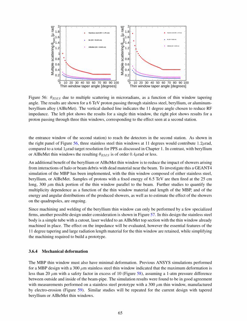
Thin window taper angle [degrees]0 10 20 30 40 50 60 70 80 90 100

rad

]µ [

RM

Sθ

Mul

tiple

sca

tterin

g

0

0.2

0.4

0.6

0.8

1

1.2

1.4

1.6

1.8

2

Stainless steel (X0 = 1.76 cm)

Be (X0 = 35.28 cm)

AlBeMet (X0 = 18.68 cm)

Thin window taper angle [degrees]0 10 20 30 40 50 60 70 80 90 100

rad

]µ [

RM

Sθ

Mul

tiple

sca

tterin

g

0

0.2

0.4

0.6

0.8

1

1.2

1.4

1.6

1.8

2

Stainless steel (X0 = 1.76 cm)

Be (X0 = 35.28 cm)

AlBeMet (X0 = 18.68 cm)

Figure 56: θRMS due to multiple scattering in microradians, as a function of thin window taperingangle. The results are shown for a 6 TeV proton passing through stainless steel, beryllium, or aluminum-beryllium alloy (AlBeMet). The vertical dashed line indicates the 11 degree angle chosen to reduce RFimpedance. The left plot shows the results for a single thin window, the right plot shows results for aproton passing through three thin windows, corresponding to the effect seen at a second station.

the entrance window of the second station) to reach the detectors in the second station. As shown inthe right panel of Figure 56, three stainless steel thin windows at 11 degrees would contribute 1.2µrad,compared to a total 1µrad target resolution for PPS as discussed in Chapter 1. In contrast, with berylliumor AlBeMet thin windows the resulting θRMS is of order 0.4µrad or less.

An additional benefit of the beryllium or AlBeMet thin window is to reduce the impact of showers arisingfrom interactions of halo or beam debris with dead material near the beam. To investigate this a GEANT4simulation of the MBP has been implemented, with the thin window composed of either stainless steel,beryllium, or AlBeMet. Samples of protons with a fixed energy of 6.5 TeV are then fired at the 25 cmlong, 300 µm thick portion of the thin window parallel to the beam. Further studies to quantify themultiplicity dependence as a function of the thin window material and length of the MBP, and of theenergy and angular distributions of the produced showers, as well as to estimate the effect of the showerson the quadrupoles, are ongoing.

Since machining and welding of the beryllium thin window can only be performed by a few specializedfirms, another possible design under consideration is shown in Figure 57. In this design the stainless steelbody is a simple tube with a cutout, laser welded to an AlBeMet top section with the thin window alreadymachined in place. The effect on the impedance will be evaluated, however the essential features of the11 degree tapering and large radiation length material for the thin window are retained, while simplifyingthe machining required to build a prototype.

3.6.4 Mechanical deformation

The MBP thin window must also have minimal deformation. Previous ANSYS simulations performedfor a MBP design with a 300 µm stainless steel thin window indicated that the maximum deformation isless than 20 µm with a safety factor in excess of 10 (Figure 58), assuming a 1-atm pressure differencebetween outside and inside of the beam-pipe. The simulation results were found to be in good agreementwith measurements performed on a stainless steel prototype with a 300 µm thin window, manufacturedby electro-erosion (Figure 59). Similar studies will be repeated for the current design with taperedberyllium or AlBeMet thin windows.

65

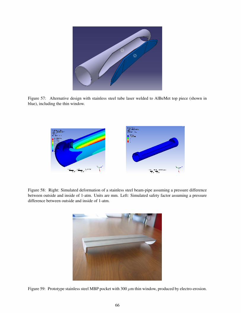
Figure 57: Alternative design with stainless steel tube laser welded to AlBeMet top piece (shown inblue), including the thin window.

Figure 58: Right: Simulated deformation of a stainless steel beam-pipe assuming a pressure differencebetween outside and inside of 1-atm. Units are mm. Left: Simulated safety factor assuming a pressuredifference between outside and inside of 1-atm.

Figure 59: Prototype stainless steel MBP pocket with 300 µm thin window, produced by electro-erosion.

66

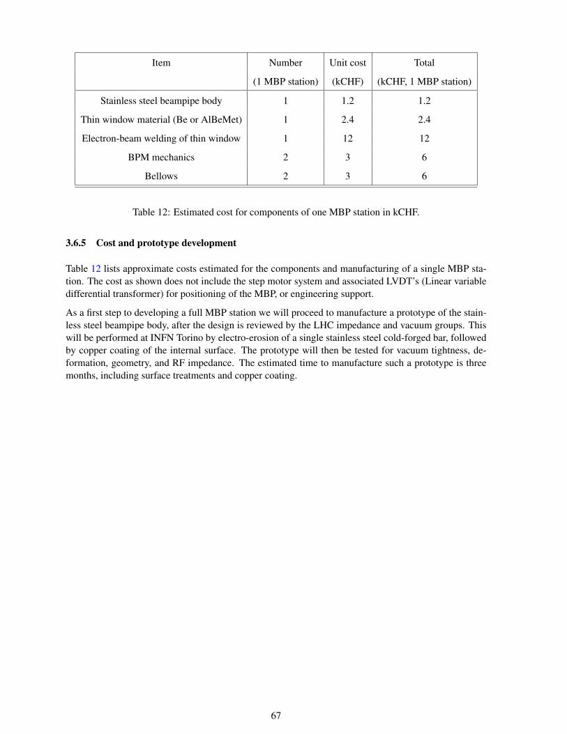
Item Number Unit cost Total

(1 MBP station) (kCHF) (kCHF, 1 MBP station)

Stainless steel beampipe body 1 1.2 1.2

Thin window material (Be or AlBeMet) 1 2.4 2.4

Electron-beam welding of thin window 1 12 12

BPM mechanics 2 3 6

Bellows 2 3 6

Table 12: Estimated cost for components of one MBP station in kCHF.

3.6.5 Cost and prototype development

Table 12 lists approximate costs estimated for the components and manufacturing of a single MBP sta-tion. The cost as shown does not include the step motor system and associated LVDT’s (Linear variabledifferential transformer) for positioning of the MBP, or engineering support.

As a first step to developing a full MBP station we will proceed to manufacture a prototype of the stain-less steel beampipe body, after the design is reviewed by the LHC impedance and vacuum groups. Thiswill be performed at INFN Torino by electro-erosion of a single stainless steel cold-forged bar, followedby copper coating of the internal surface. The prototype will then be tested for vacuum tightness, de-formation, geometry, and RF impedance. The estimated time to manufacture such a prototype is threemonths, including surface treatments and copper coating.

67

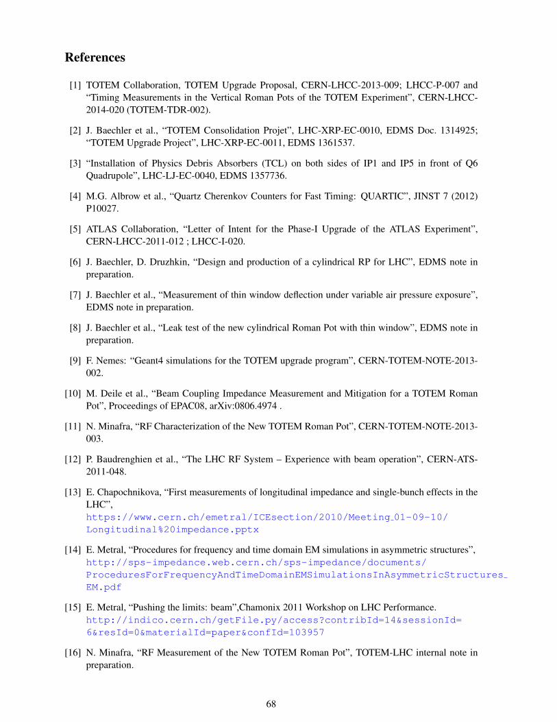
References

[1] TOTEM Collaboration, TOTEM Upgrade Proposal, CERN-LHCC-2013-009; LHCC-P-007 and“Timing Measurements in the Vertical Roman Pots of the TOTEM Experiment”, CERN-LHCC-2014-020 (TOTEM-TDR-002).

[2] J. Baechler et al., “TOTEM Consolidation Projet”, LHC-XRP-EC-0010, EDMS Doc. 1314925;“TOTEM Upgrade Project”, LHC-XRP-EC-0011, EDMS 1361537.

[3] “Installation of Physics Debris Absorbers (TCL) on both sides of IP1 and IP5 in front of Q6Quadrupole”, LHC-LJ-EC-0040, EDMS 1357736.

[4] M.G. Albrow et al., “Quartz Cherenkov Counters for Fast Timing: QUARTIC”, JINST 7 (2012)P10027.

[5] ATLAS Collaboration, “Letter of Intent for the Phase-I Upgrade of the ATLAS Experiment”,CERN-LHCC-2011-012 ; LHCC-I-020.

[6] J. Baechler, D. Druzhkin, “Design and production of a cylindrical RP for LHC”, EDMS note inpreparation.

[7] J. Baechler et al., “Measurement of thin window deflection under variable air pressure exposure”,EDMS note in preparation.

[8] J. Baechler et al., “Leak test of the new cylindrical Roman Pot with thin window”, EDMS note inpreparation.

[9] F. Nemes: “Geant4 simulations for the TOTEM upgrade program”, CERN-TOTEM-NOTE-2013-002.

[10] M. Deile et al., “Beam Coupling Impedance Measurement and Mitigation for a TOTEM RomanPot”, Proceedings of EPAC08, arXiv:0806.4974 .

[11] N. Minafra, “RF Characterization of the New TOTEM Roman Pot”, CERN-TOTEM-NOTE-2013-003.

[12] P. Baudrenghien et al., “The LHC RF System – Experience with beam operation”, CERN-ATS-2011-048.

[13] E. Chapochnikova, “First measurements of longitudinal impedance and single-bunch effects in theLHC”,https://www.cern.ch/emetral/ICEsection/2010/Meeting 01-09-10/Longitudinal%20impedance.pptx

[14] E. Metral, “Procedures for frequency and time domain EM simulations in asymmetric structures”,http://sps-impedance.web.cern.ch/sps-impedance/documents/ProceduresForFrequencyAndTimeDomainEMSimulationsInAsymmetricStructuresEM.pdf

[15] E. Metral, “Pushing the limits: beam”,Chamonix 2011 Workshop on LHC Performance.http://indico.cern.ch/getFile.py/access?contribId=14&sessionId=6&resId=0&materialId=paper&confId=103957

[16] N. Minafra, “RF Measurement of the New TOTEM Roman Pot”, TOTEM-LHC internal note inpreparation.

68

https://www.cern.ch/emetral/ICEsection/2010/Meeting_01-09-10/Longitudinal%20impedance.pptx

https://www.cern.ch/emetral/ICEsection/2010/Meeting_01-09-10/Longitudinal%20impedance.pptx

http://sps-impedance.web.cern.ch/sps-impedance/documents/ProceduresForFrequencyAndTimeDomainEMSimulationsInAsymmetricStructures_EM.pdf



http://indico.cern.ch/getFile.py/access?contribId=14&sessionId=6&resId=0&materialId=paper&confId=103957

http://indico.cern.ch/getFile.py/access?contribId=14&sessionId=6&resId=0&materialId=paper&confId=103957

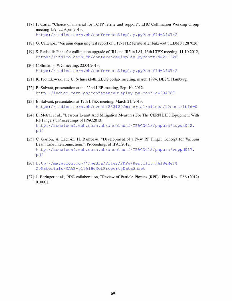
[17] F. Carra, “Choice of material for TCTP ferrite and support”, LHC Collimation Working Groupmeeting 159, 22 April 2013.https://indico.cern.ch/conferenceDisplay.py?confId=246742

[18] G. Cattenoz, “Vacuum degassing test report of TT2-111R ferrite after bake-out”, EDMS 1287626.

[19] S. Redaelli: Plans for collimation upgrade of IR1 and IR5 in LS1, 13th LTEX meeting, 11.10.2012,https://indico.cern.ch/conferenceDisplay.py?confId=211226

[20] Collimation WG meeting, 22.04.2013,https://indico.cern.ch/conferenceDisplay.py?confId=246742

[21] K. Piotrzkowski and U. Schneekloth, ZEUS collab. meeting, march 1994, DESY, Hamburg.

[22] B. Salvant, presentation at the 22nd LEB meeting, Sep. 10, 2012.http://indico.cern.ch/conferenceDisplay.py?confId=204787

[23] B. Salvant, presentation at 17th LTEX meeting, March 21, 2013.https://indico.cern.ch/event/233129/material/slides/1?contribId=0

[24] E. Metral et al., ”Lessons Learnt And Mitigation Measures For The CERN LHC Equipment WithRF Fingers”, Proceedings of IPAC2013.http://accelconf.web.cern.ch/accelconf/IPAC2013/papers/tupwa042.pdf

[25] C. Garion, A. Lacroix, H. Rambeau, ”Development of a New RF Finger Concept for VacuumBeam Line Interconnections”, Proceedings of IPAC2012.http://accelconf.web.cern.ch/accelconf/IPAC2012/papers/weppd017.pdf

[26] http://materion.com/∼/media/Files/PDFs/Beryllium/AlBeMet%20Materials/MAAB-017AlBeMetPropertyDataSheet

[27] J. Beringer et al., PDG collaboration, ”Review of Particle Physics (RPP)” Phys.Rev. D86 (2012)010001.

69

https://indico.cern.ch/conferenceDisplay.py?confId=246742



http://indico.cern.ch/conferenceDisplay.py?confId=204787

https://indico.cern.ch/event/233129/material/slides/1?contribId=0

http://accelconf.web.cern.ch/accelconf/IPAC2013/papers/tupwa042.pdf

http://accelconf.web.cern.ch/accelconf/IPAC2013/papers/tupwa042.pdf

http://accelconf.web.cern.ch/accelconf/IPAC2012/papers/weppd017.pdf

http://accelconf.web.cern.ch/accelconf/IPAC2012/papers/weppd017.pdf

http://materion.com/~/media/Files/PDFs/Beryllium/AlBeMet%20Materials/MAAB-017AlBeMetPropertyDataSheet

http://materion.com/~/media/Files/PDFs/Beryllium/AlBeMet%20Materials/MAAB-017AlBeMetPropertyDataSheet

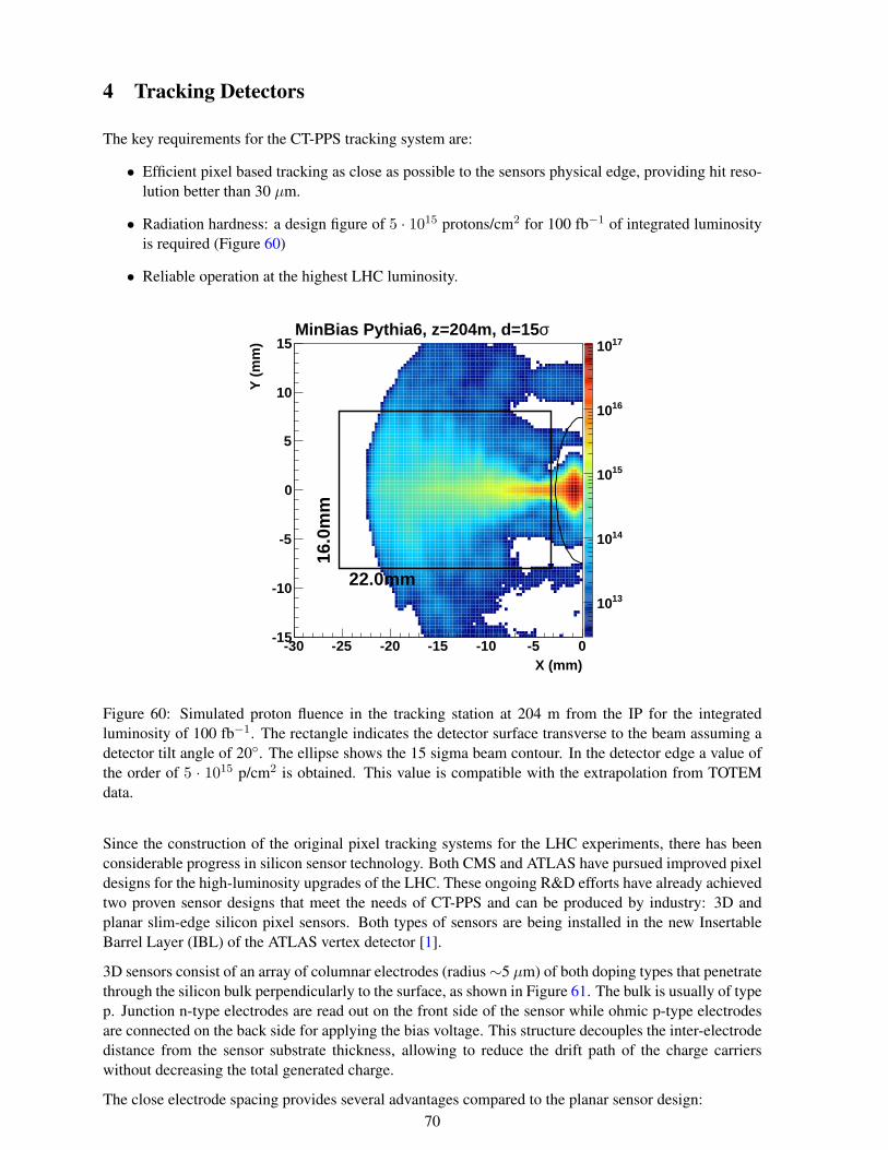
4 Tracking Detectors

The key requirements for the CT-PPS tracking system are:

• Efficient pixel based tracking as close as possible to the sensors physical edge, providing hit reso-lution better than 30 µm.

• Radiation hardness: a design figure of 5 · 1015 protons/cm2 for 100 fb−1 of integrated luminosityis required (Figure 60)

• Reliable operation at the highest LHC luminosity.

X (mm)-30 -25 -20 -15 -10 -5 0

Y (

mm

)

-15

-10

-5

0

5

10

15

1310

1410

1510

1610

1710σMinBias Pythia6, z=204m, d=15

22.0mm

16.0

mm

Figure 60: Simulated proton fluence in the tracking station at 204 m from the IP for the integratedluminosity of 100 fb−1. The rectangle indicates the detector surface transverse to the beam assuming adetector tilt angle of 20. The ellipse shows the 15 sigma beam contour. In the detector edge a value ofthe order of 5 · 1015 p/cm2 is obtained. This value is compatible with the extrapolation from TOTEMdata.

Since the construction of the original pixel tracking systems for the LHC experiments, there has beenconsiderable progress in silicon sensor technology. Both CMS and ATLAS have pursued improved pixeldesigns for the high-luminosity upgrades of the LHC. These ongoing R&D efforts have already achievedtwo proven sensor designs that meet the needs of CT-PPS and can be produced by industry: 3D andplanar slim-edge silicon pixel sensors. Both types of sensors are being installed in the new InsertableBarrel Layer (IBL) of the ATLAS vertex detector [1].

3D sensors consist of an array of columnar electrodes (radius∼5 µm) of both doping types that penetratethrough the silicon bulk perpendicularly to the surface, as shown in Figure 61. The bulk is usually of typep. Junction n-type electrodes are read out on the front side of the sensor while ohmic p-type electrodesare connected on the back side for applying the bias voltage. This structure decouples the inter-electrodedistance from the sensor substrate thickness, allowing to reduce the drift path of the charge carrierswithout decreasing the total generated charge.

The close electrode spacing provides several advantages compared to the planar sensor design:70

Figure 61: Sketch of a 3D sensor.

• low full depletion voltage (∼10 V),

• fast charge collection time,

• reduced charge-trapping probability and therefore high radiation hardness.

As a result, 3D detectors are emerging as one of the most promising technologies for the innermost layersof tracking devices for the foreseen upgrades of the LHC. A very interesting feature of 3D technologyis the possibility of realizing the so-called “active edge” [4], i.e. a deep trench all around the sensor thatreduces the dead region to a few microns from the physical edge of the device, compared to the hundredsof µm for standard planar detectors.

As a backup solution, we have identified a second sensor concept, a slim-edge planar design produced byCIS (tested by ATLAS) and SINTEF (tested by CMS), based on a more mature fabrication process. Wehave designed the CT-PPS sensor readout and packaging to accept either sensors as a drop-in replace-ment.

The chosen configuration for the tracking system consists of two detector stations in each arm, for a totalof four detector stations. These are the horizontal RPs located at ∼210 m. Each station will contain onestack of silicon tracking detectors. Each stack will consist of six planes, where each plane contains a1.6×2.4 cm2 pixel sensor read out by six PSI46dig readout chips ROCs [2]. Each ROC reads 52×80pixels with dimensions 150×100 µm2. Given the small area of the detector, covered by a small numberof individual sensors, we have chosen a number of planes that provide confortable redundancy makingthe system resilient to possible failures. The design of the front-end electronics and of the DAQ is basedon that developed for the Phase 1 upgrade of the CMS silicon pixel detectors [3].

The resolution of the x-coordinate is determined by the sharing of charge in the pixel clusters, whichdepends on the detector tilt angle in the x-z plane. While this parameter is not yet defined, test beamresults with similar sensors indicate that for an angle of 20 degrees the two-pixel clusters have resolutionof the order of 10 µm. Since there is no tilt in the y-z plane, the resolution of the y-coordinate is of theorder of 30 µm.

4.1 Silicon sensors

4.1.1 Baseline solution: 3D silicon sensors

The baseline CT-PPS tracking system is based on 3D pixel sensors, produced either by FBK (Trento,Italy) or CNM (Barcelona, Spain), which we think provide the best performance in terms of activeregion and radiation hardness. These companies have already produced 200 µm slim-edge 3D sensorsfor the IBL project with satisfactory yield. However, for CT-PPS we would like to pursue the option witha 100 µm, or better, slim-edge design, where the active region of the sensor is as close as 100 µm to the

71

edge. Since such slim edges have not yet been produced, we mitigated our schedule risk by designing theCT-PPS tracking system to allow rapid installation, or replacement, of the unit during a LHC technicalstop.

The three-dimensional (3D) architecture for radiation-hard silicon sensors was first proposed by Parker,Kenney and Segal in 1997 [5]. The first 3D devices with fully passing-through electrodes were producedby the Stanford Nano-fabrication Facility (Stanford, USA) [6] and the fabrication process was furtherdeveloped at SINTEF (Oslo, Norway) [7] for larger-scale production. This fabrication process is single-sided, with the electrodes all initially formed (drilled) on the same side. It allows the fabrication of activeedges but it requires a support wafer, which is difficult to remove. To avoid this problem, two other3D producers, FBK (Trento, Italy) and CNM (Barcelona, Spain), independently developed a differenttechnique without a support wafer [8, 9]. A double-sided fabrication technology is used, with junctionelectrodes etched from the front side and ohmic electrodes etched from the back side. These two vendors(FBK and CNM) have produced 3D sensors for the ATLAS IBL project, either with fully passing-throughor with partially passing-through electrodes, respectively [10], and with a dead region of 200 µm fromthe sensor’s edge (slim edge).

The particular structure of 3D sensors has a few drawbacks also: the fabrication process is more com-plicated and requires more steps with respect to the production of planar silicon detectors; the shortelectrode distance and the extension inside the bulk increase the pixel capacitance and, consequently, thenoise induced on the readout electronics. Moreover, the response is not completely uniform because ofthe electrodes, which are less efficient or completely inefficient regions, depending on the fabricationprocess. Nevertheless, the fact that 3D sensors passed the requirements imposed by the stringent IBLenvironment [11] is an indication that these drawbacks can be overcome. The ATLAS 3D Collaborationmeasured the efficiency of these detectors in several test beams and found it to be well above 99% [10].Because of the electrode geometry, 3D devices exhibit some loss of tracking efficiency for normal inci-dent tracks but recover full efficiency with tilted tracks, or equivalently by tilting the detectors. Moreover,only minor degradation was observed after irradiation [12].

CMS-compatible sensors have been fabricated by SINTEF, FBK and CNM. Three different electrodeconfigurations were manufactured up to now:

• single n-type electrode (1E),

• two n-type electrodes (2E), and

• four n-type electrodes (4E) per pixel cell.

The distance between n-type and p-type electrodes is of great importance since it affects parameterssuch as capacitance and noise, depletion voltage, charge collection, and radiation hardness. The inter-electrode distances in the 1E, 2E, and 4E configurations are 90, 62.5, and 45 µm, respectively. Sensorthicknesses varied between 200 and 230 µm.

Testing of these devices has been carried out together with the CMS pixel upgrade group, which isalso exploring this novel technology. Several CNM and FBK sensors with standard guard rings or slimedges, and with different electrode configurations were characterized in the laboratory [13] and testedat Fermilab with a proton beam of 120 GeV. Data were taken for various values of depletion voltages,read-out electronics thresholds, temperatures and angles with respect to the beam. Some of these deviceswere irradiated at Los Alamos National Laboratory (USA) with 800 MeV protons at fluences up to1015 neq/cm2 and re-tested [14]. Results showed the best performance for the 2E configuration. For allthe above measurements 3D sensors were read out with the PSI46 analog chip [15] presently used in theCMS pixel tracking detectors.

Recently (May 2014), in a test beam at Fermilab, seven un-irradiated FBK 1E 3D sensors, processed inthe framework of the ATLAS IBL production [16], with 200 µm slim edges [17], have been tested cou-pled to the new PSI46dig ROC, developed for the Phase 1 upgrade of the CMS pixel tracking detectors.

72

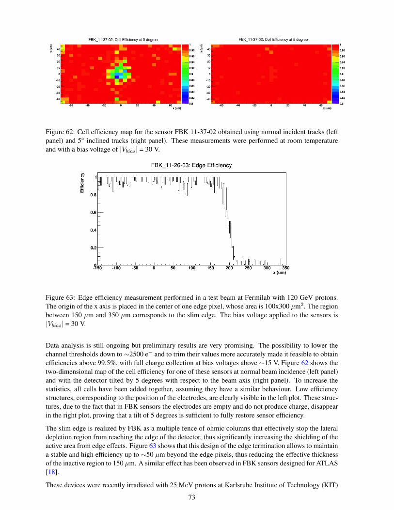
Figure 62: Cell efficiency map for the sensor FBK 11-37-02 obtained using normal incident tracks (leftpanel) and 5 inclined tracks (right panel). These measurements were performed at room temperatureand with a bias voltage of |Vbias| = 30 V.

Figure 63: Edge efficiency measurement performed in a test beam at Fermilab with 120 GeV protons.The origin of the x axis is placed in the center of one edge pixel, whose area is 100x300 µm2. The regionbetween 150 µm and 350 µm corresponds to the slim edge. The bias voltage applied to the sensors is|Vbias| = 30 V.

Data analysis is still ongoing but preliminary results are very promising. The possibility to lower thechannel thresholds down to ∼2500 e− and to trim their values more accurately made it feasible to obtainefficiencies above 99.5%, with full charge collection at bias voltages above ∼15 V. Figure 62 shows thetwo-dimensional map of the cell efficiency for one of these sensors at normal beam incidence (left panel)and with the detector tilted by 5 degrees with respect to the beam axis (right panel). To increase thestatistics, all cells have been added together, assuming they have a similar behaviour. Low efficiencystructures, corresponding to the position of the electrodes, are clearly visible in the left plot. These struc-tures, due to the fact that in FBK sensors the electrodes are empty and do not produce charge, disappearin the right plot, proving that a tilt of 5 degrees is sufficient to fully restore sensor efficiency.

The slim edge is realized by FBK as a multiple fence of ohmic columns that effectively stop the lateraldepletion region from reaching the edge of the detector, thus significantly increasing the shielding of theactive area from edge effects. Figure 63 shows that this design of the edge termination allows to maintaina stable and high efficiency up to ∼50 µm beyond the edge pixels, thus reducing the effective thicknessof the inactive region to 150 µm. A similar effect has been observed in FBK sensors designed for ATLAS[18].

These devices were recently irradiated with 25 MeV protons at Karlsruhe Institute of Technology (KIT)

73

Figure 64: Schematic of the active edge as implemented by VTT for planar sensors.

to 4 different fluences (1·1015 neq/cm2, 3·1015 neq/cm2, 6·1015 neq/cm2 and 1·1016 neq/cm2) and arecurrently being characterized in laboratory. The level of the leakage current measured at −10C isacceptable (∼80 µA for sensors irradiated to 1·1015 neq/cm2). A significant increase of the breakdownvoltage (|VBD| ∼35 V before irradiation) has been observed: the devices irradiated at the lower fluencereach a maximum operating voltage of |Vbias| ∼ 80 V, while the ones at the larger fluence exceed 120 V.These values of breakdown voltage should be sufficiently high to allow to operate the sensors at theoptimal bias also after irradiation.A test beam at Fermilab is foreseen for the second half of August 2014 to perform further studies on thebehaviour of irradiated detectors.

4.1.2 Alternative solutions: slim-edge planar sensors

In the past years a large effort went into studying strip and pixel planar sensors with slim edges, as theyallow for a simplified tracker geometry with respect of traditional wide-edge sensors [19, 20] and theycan instrument larger areas than what is possible to achieve with 3D slim-edge sensors.

The key factor determining the inactive edge extension are the defects introduced by detector dicingwith diamond saws, which originate increased leakage currents and decreased breakdown voltages if thedepletion region approaches the physical edge of the sensor. Therefore, the first approach to slim-edgesensors has been to improve the quality of the lateral cut, using laser dicing in combination with chemicaletching. This technique, however, did not manage to obtain the results that were hoped for.

A second strategy relies on thin sensors: as the lateral field extends for a fraction of the sensors thickness,thin sensors are well suited to obtain slim edges. If a detector is 100 µm thick, the inactive edge is roughlyof the same extension.

A completely different approach has been obtained by the introduction of active edges, proposed bythe Stanford Nanofabrication Facility (SNF) for 3D detector technology [4] and later applied also toplanar sensors [21]. In this design, the problems connected with the surface defects at the edge of thesensor are avoided by making the edge an active component in the definition of the electric field, asshown in Figure 64: the boron implant does not stop at the backplane, but continues along the detectoredges, reaching the frontplane. Using this technique, the ATLAS Planar Pixel Sensor Collaboration hasmanufactured several prototypes with 50 and 100 µm slim edge or active edge.

An interesting alternative to the active-edge approach is based on a special treatment of the sensor edgevia the sequence of three steps: scribing, cleaving and passivation [22]. Wafer scribing and cleavingare used to minimize the number of defects with respect to a standard dicing saw, whereas edge surfacepassivation aims at allowing for a bias voltage gradient along the sidewall surface, pratically turning theedge into a large resistor. This technique has the advantage that it can be used in post-production toobtain slim-edge sensors from finished wide-edge sensors.

74

With these techniques, slim- and active-edge planar sensors are reaching the same performance as 3Dsensors, and represent viable fall back solutions.

4.2 The readout system

The readout of the pixel detector is largely based on components developed in the framework of thePixel Upgrade Phase 1 readout project. This readout chain has been proven to work efficiently. Mostcomponents are currently at an advanced test stage and/or in final production. In this section, an overviewof the readout system of the pixel detector is given shortly with special emphasis on CT-PPS specificpoints. Extensive documentation of each component can be obtained elsewhere [3].

The complete readout chain of one detector package is shown in Figure 65. By convention a detectorpackage is a set of six modules, one for each sensor present in a RP. There are in total four detectorpackages. The specific CT-PPS elements in the readout system are the six RPix Modules (Roman PotPIXel Modules) and the RPix Portcard. The low voltage system and high voltage system are part of thelow voltage and high voltage system of TOTEM, already in place. The backend DAQ electronics, to beinstalled in the service cavern, is being actively developed by CMS as part of the Pixel Upgrade Phase 1project.

Figure 65: Detector readout and control strings. All components up to PP1 are in the LHC tunnel, whileFEDs and FECs are in the service cavern.

Each RPix Module consists of a flexible hybrid circuit hosting: a silicon sensor, six ROCs “bump-bonded” to the silicon sensor, and one Token Bit Manager (TBM) chip. The ROC is responsible forcharge collection, charge discrimination and data sparsification. Two slightly different versions of thechip, named V2.1 and V2.1b, are suitable: which version to use is currently under evaluation.

The TBM is responsible for reading out the six ROCs in the module (it can manage up to 16) using atoken ring protocol and serialising the data over a single output line. The TBM versions suitable for

75

this application, named TBM08a and TBM08b, manage two token bit ring protocols at the same time,multiplexing the two data streams on the same output line before encoding the data stream using a 4B/5BNRZI schema. The net result is an uplink data stream running at 400 Mb/s. Dispatching these high speedsignals on the flexible hybrid without degrading them is one of the major design requirements of theRPix Module, together with the need to deliver the high voltage to the sensor safely.

The RPix Portcard accomplishes a variety of tasks. The board receives the output data from six RPixmodules and retransmits them on six optical fibres towards DAQ modules, using a POH7 opto-electricalconverter mezzanine card [23]. This board also receives fast configuration commands from the Pixel FECvia optical fibres, translates these signals using detector optical receivers (DOH) and dispatches them tothe modules. These functionality are similar to those of the Forward Pixel project portcard developed byFermilab. Moreover the RPix Portcard integrates other components such as the radiation sensors, part ofthe TOTEM DCS radiation monitoring system, and the CMS Tracker Optical Control Link componentswhich are capable of receiving and decoding the commands sent from the Tracker FEC. Finally, thenewly developed DC/DC converters [24], developed by CMS, are installed on the board, in order togenerate the different voltages needed by the portcard itself and by the attached modules.

For the backend DAQ system, the plan is to use the new uTCA crates and boards developed for the PixelUpgrade Phase 1 project. A fallback solution, using VME electronics, is available in case the baselinesolution could suffer long delays.

It should be noted that the tracking front-end based on the CMS pixel readout chip PSI46dig chip doesnot have trigger outputs and therefore can not be integrated in the L1 Trigger.

4.3 The detector assembly

The mechanical structure of the detector is designed so as to ensure a positioning accuracy comparableto the resolution of the detector and at the same time provide a proper thermal conductance for detectorcooling. The material budget of the mechanical structure is not an issue, except for the area below thesensors, since most of the support is outside of the tracks path. Stiffness and thermal properties are morerelevant. Moreover a desirable feature is the integration with the present cooling system.

The sensor planes are not mounted perpendicular to the beam direction: they are rotated by 18.5 degreesaround the vertical axis. This angle is enough to remove the geometrical inefficiency, due to presence ofthe columnar electrodes in the 3D sensors, and guarantees optimal resolution in the horizontal directionthanks to charge sharing between nearby pixels.

An exploded view of one module is shown in Figure 66. Each module consists of several different parts.The support plate, consisting of two layers of different materials, can be seen at the bottom. The first,1.25 mm thick, layer is made of CE7, a controlled expansion material composed of 70% Si and 30% Al.The second, 0.7 mm thick, layer is made of Thermal Pyrolithic Graphite (TPG), a low density materialconsisting of stacked graphite sheets and featuring an extremely high thermal conductivity on the sheetsplane.

A long kapton flexible hybrid circuit is glued on top of the TPG layer, as well as the silicon detector,“bump-bonded” to six readout chips. Wire bonds provide electrical contacts between detector pads andhybrid electric lines. The flexible circuit hosts the TBM and provides connection, at the other end, to thereadout board.

An exploded view of one detector package is shown in Figure 67. Pairs of modules are screwed faceto face to two aluminium support bars, each one machined in a single piece to ensure the best thermalcontact. These bars are in tight contact with the cooling pipes. The detector assembly is modular.Mechanics is arranged in such a way that when the modular pieces are brought together they enclose thecooling pipes and the detector package is complete. In order to maximise heat exchange, each TPG is in

76

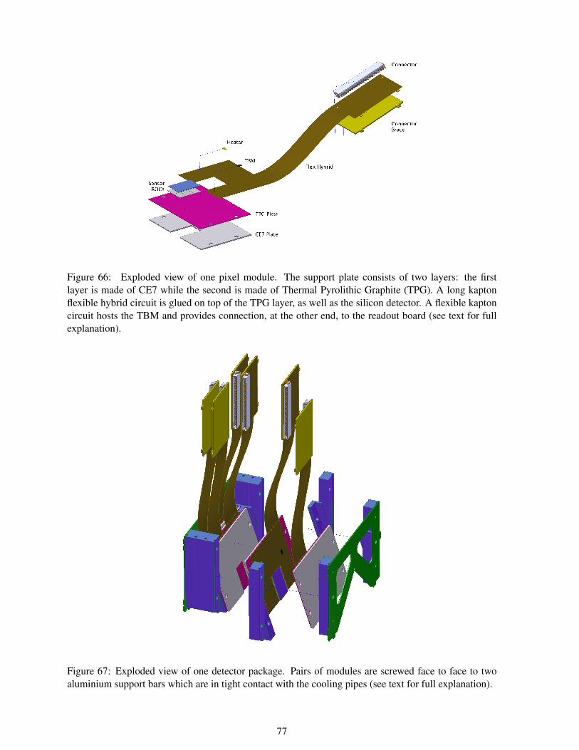
Figure 66: Exploded view of one pixel module. The support plate consists of two layers: the firstlayer is made of CE7 while the second is made of Thermal Pyrolithic Graphite (TPG). A long kaptonflexible hybrid circuit is glued on top of the TPG layer, as well as the silicon detector. A flexible kaptoncircuit hosts the TBM and provides connection, at the other end, to the readout board (see text for fullexplanation).

Figure 67: Exploded view of one detector package. Pairs of modules are screwed face to face to twoaluminium support bars which are in tight contact with the cooling pipes (see text for full explanation).

77

Figure 68: Overview of the RP inner volume. Detectors, coloured in blue, are hosted in the rectangularbox at the bottom of the picture. The cooling lines are coloured in red. The RP readout board is visiblein the right most picture. It is glued on the feed-through of the flange; only the connectors are visible,most of it extension is above the flange.

direct contact with the ROCs and the aluminium supports.

The readout board (see Figure 68) will be attached on the feedthrough of the flange between normalenvironment and secondary vacuum. Only the connectors will protrude into the secondary vacuum inorder to connect to the detector package. Enough space exists on top of the flange to host the rest of theboard.

A thermal prototype of one detector package will be assembled in order to test the conceptual design,the choice of the materials and the fluid-dynamical parameters of the cooling system. The ROCs willbe replaced with heaters with equivalent power density. The prototype will be fixed to a vacuum cham-ber flange and inserted in an experimental vacuum chamber. All the connections of the pressure andtemperature sensors will be read out through a vacuum feed-through.

4.4 The cooling system

The existing cooling system [25] is suitable to host the pixel detectors inside the pot. The requirementsimposed by the pixel detector (< 10W per package, ∼ −20 0C) are very similar to those imposed by thesilicon microstrip detector (< 20W per package, ∼ −10 0C). The main difference is the region wheremost of the heat is produced.

The system is designed to remove a thermal load from sensors, electronics and RF coupling up to∼ 50 Wper pot. In the case of the Roman Pot equipped with the RF cylindrical collar shield, the power released

78

Figure 69: Temperature distribution measured on test points on the silicon micro-strip detectors hybridsfor a heating power of 2 W and 3 W (open and solid markers respectively), compared with the evaporatortemperature.

in the pot, due to residual RF coupling with the beam, is expected to be 10 W when the pot approachesthe beam to 1 mm.

Because of the high radiation environment of the LHC tunnel, the main part of the refrigeration systemis installed in the underground service area USC55 at IP5, a protected and always accessible place. An“fluorocarbon evaporative” cooling [26] strategy has been adopted since it can transport fluid at ambienttemperature over long distances (from USC55 near IP5 to the RP stations at 210 m and 220 m) withoutheat losses. The fluid is supplied in liquid phase and at high pressure at the RP circuit inlet. Thethrottling of the fluid is done in the pot and is based on metal capillary tubes. An isenthalpic expansionprocess through capillaries decreases its pressure and tunes the temperature to the design evaporationvalue of −30 0C. The C3F8 fluorocarbon dielectric fluid has been selected because it is non-flammable,non-conductive and radiation resistant.

Inside the RP the cooling fluid flows through thin-walled copper-nickel pipes of 2.5 mm outer diame-ter. Two independent pipe evaporators supply fluid to the right and left side of the detector package.The evaporators, mechanically coupled to the detector package, are decoupled from the rest of the cool-ing system at the inputs and outputs by bellows. They are shaped in a double-S configuration and aresqueezed in between the frame structure which foresees precisely machined grooves for this purpose.The evaporators are fed by capillary tubes that provide the throttling of the fluid. The coolant in gasphase is exhausted via larger diameter pipes. Both the capillaries and the exhausting pipes enter andleave the pot through two vacuum feed-throughs.

For the current frame structure, supporting 10 planes of micro-strip detectors, the measurements showthat for an heating power of 2 W per plane the temperature spread on a single hybrid card is within 3 0C,and the maximum temperature difference between detectors is less than 10 0C (Figure 69). We expect toget similar or better results for the new six plane frame structure designed for the pixel detectors.

79

References

[1] ATLAS Insertable B-Layer Technical Design Report, ATLAS IBL Collaboration, CERN-LHCC-2010-013, ATLAS-TDR-19, 15 September 2010 (2010).

[2] H.Chr. Kastli, “Frontend electronics development for the CMS pixel detector upgrade”, Nucl. Instr.and Meth. A 731 (2013) 88.

[3] CMS Technical Design Report for the Pixel Detector Upgrade, CMS Collaboration, CERN-LHCC-2012-016; CMS-TDR-11, 7 September 2012 (2012).

[4] C.J. Kenney et al., “Results From 3-D Silicon Sensors With Wall Electrodes: Near-Cell-Edge Sen-sitivity Measurements as a Preview of Active-Edge Sensors”, IEEE Trans. Nucl. Sci. 48 (2001)2405.

[5] S.I. Parker et al., “3D - A proposed new architecture for solid-state radiation detectors”, Nucl. Instr.and Meth. A 395 (1997) 328.

[6] C.J. Kenney et al., “Silicon Detectors with 3-D Electrode Arrays: Fabrication and Initial Test Re-sults”, IEEE Trans. Nucl. Sci. 46 (1999) 1224.

[7] T.E. Hansen et al., “First fabrication of full 3D-detectors at SINTEF”, JINST 4 (2009) P03010.

[8] A. Zoboli et al., “Double-Sided, Double-Type-Column 3-D Detectors: Design, Fabrication, andTechnology Evaluation”, IEEE Trans. Nucl. Sci. 55 (2008) 2775.

[9] G. Pellegrini et al., “First double-sided 3-D detectors fabricated at CNM-IMB”, Nucl. Instr. andMeth. A 592 (2008) 38.

[10] The ATLAS IBL Collaboration, “Prototype ATLAS IBL modules using the FE-I4A front-end read-out chip”, JINST 7 (2012) P11010.

[11] C. Da Via et al., “3D active edge silicon sensors: Device processing, yield and QA for the ATLAS-IBL production”, Nucl. Instr. and Meth. A 699 (2013) 18.

[12] A. Micelli et al., “3D-FBK pixel sensors: Recent beam tests results with irradiated devices”, Nucl.Instr. and Meth. A 650 (2011) 150.

[13] E. Alagoz et al., “Simulation and laboratory test results of 3D CMS pixel detectors for HL-LHC”,JINST 7 (2012) P08023.

[14] M. Obertino et al., “Performance of CMS 3D silicon pixel detectors before and after irradiation”,Nucl. Instr. and Meth. A 730 (2013) 33;M. Bubna et al., “Testbeam and laboratory test results of irradiated 3D CMS pixel detectors”, Nucl.Instr. and Meth. A 732 (2013) 52;A. Krzywda et al., “Pre- and post-irradiation performance of FBK 3D silicon pixel detectors forCMS”, Nucl. Instr. and Meth. A 763 (2014) 404.

[15] H.Chr. Kastli et al., “Design and performance of the CMS pixel detector readout chip”, Nucl. Instr.and Meth. A 565 (2006) 188.

[16] C. Da Via et al., “3D silicon sensors: Design, large area production and quality assurance for theATLAS IBL pixel detector upgrade”, Nucl. Instr. and Meth. A 694 (2012) 321.

[17] M. Povoli et al., “Slim edges in double-sided silicon 3D detectors”, JINST 7 (2012) C01015.

[18] J. Lange, “3D silicon pixel detectors for the ATLAS Forward Physics experiment”, 9th TrentoWorkshop on Advanced Silicon Radiation Detectors (2014).

80

[19] http://pos.sissa.it/archive/conferences/198/042/Vertex2013 042.pdf.

[20] https://indico.cern.ch/event/265941/

[21] C.J. Kenney et al., “Active-edge planar radiation sensors”, Nucl. Instr. and Meth. A 565 (2006) 272.

[22] V. Fadeyev et al., “Scribe-cleave-passivate (SCP) slim edge technology for silicon sensors”, Nucl.Instr. and Meth. A 731 (2013) 260.

[23] J. Troska et al., “Prototype pixel optohybrid for the CMS phase 1 upgraded pixel detector”, JINST7 (2012) C01113.

[24] L. Feld et al., “Development of a DC-DC conversion powering scheme for the CMS Phase-1 pixelupgrade”, JINST 9 (2014) C01048.

[25] The TOTEM Collaboration, G. Anelli et al., “The TOTEM Experiment at the CERN Large HadronCollider”, JINST 3 (2008) S08007.

[26] V. Vacek et al., “Perfluorocarbons and their use in cooling systems for semiconductor particledetectors”, Fluid Phase Equil. 174 (2000) 191.

81

http://pos.sissa.it/archive/conferences/198/042/Vertex2013_042.pdf

http://pos.sissa.it/archive/conferences/198/042/Vertex2013_042.pdf

https://indico.cern.ch/event/265941/

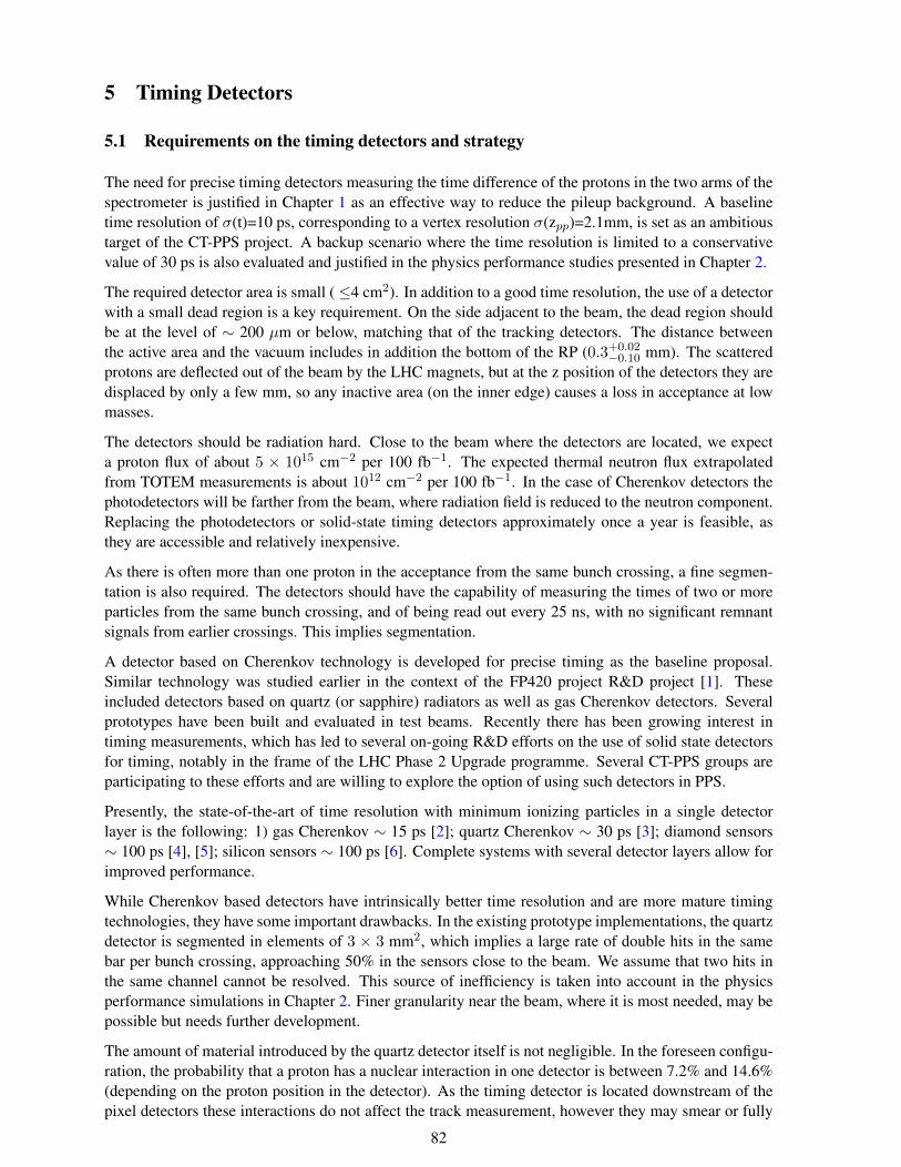
5 Timing Detectors

5.1 Requirements on the timing detectors and strategy

The need for precise timing detectors measuring the time difference of the protons in the two arms of thespectrometer is justified in Chapter 1 as an effective way to reduce the pileup background. A baselinetime resolution of σ(t)=10 ps, corresponding to a vertex resolution σ(zpp)=2.1mm, is set as an ambitioustarget of the CT-PPS project. A backup scenario where the time resolution is limited to a conservativevalue of 30 ps is also evaluated and justified in the physics performance studies presented in Chapter 2.

The required detector area is small (≤4 cm2). In addition to a good time resolution, the use of a detectorwith a small dead region is a key requirement. On the side adjacent to the beam, the dead region shouldbe at the level of ∼ 200 µm or below, matching that of the tracking detectors. The distance betweenthe active area and the vacuum includes in addition the bottom of the RP (0.3+0.02

−0.10 mm). The scatteredprotons are deflected out of the beam by the LHC magnets, but at the z position of the detectors they aredisplaced by only a few mm, so any inactive area (on the inner edge) causes a loss in acceptance at lowmasses.

The detectors should be radiation hard. Close to the beam where the detectors are located, we expecta proton flux of about 5 × 1015 cm−2 per 100 fb−1. The expected thermal neutron flux extrapolatedfrom TOTEM measurements is about 1012 cm−2 per 100 fb−1. In the case of Cherenkov detectors thephotodetectors will be farther from the beam, where radiation field is reduced to the neutron component.Replacing the photodetectors or solid-state timing detectors approximately once a year is feasible, asthey are accessible and relatively inexpensive.

As there is often more than one proton in the acceptance from the same bunch crossing, a fine segmen-tation is also required. The detectors should have the capability of measuring the times of two or moreparticles from the same bunch crossing, and of being read out every 25 ns, with no significant remnantsignals from earlier crossings. This implies segmentation.

A detector based on Cherenkov technology is developed for precise timing as the baseline proposal.Similar technology was studied earlier in the context of the FP420 project R&D project [1]. Theseincluded detectors based on quartz (or sapphire) radiators as well as gas Cherenkov detectors. Severalprototypes have been built and evaluated in test beams. Recently there has been growing interest intiming measurements, which has led to several on-going R&D efforts on the use of solid state detectorsfor timing, notably in the frame of the LHC Phase 2 Upgrade programme. Several CT-PPS groups areparticipating to these efforts and are willing to explore the option of using such detectors in PPS.

Presently, the state-of-the-art of time resolution with minimum ionizing particles in a single detectorlayer is the following: 1) gas Cherenkov ∼ 15 ps [2]; quartz Cherenkov ∼ 30 ps [3]; diamond sensors∼ 100 ps [4], [5]; silicon sensors ∼ 100 ps [6]. Complete systems with several detector layers allow forimproved performance.

While Cherenkov based detectors have intrinsically better time resolution and are more mature timingtechnologies, they have some important drawbacks. In the existing prototype implementations, the quartzdetector is segmented in elements of 3 × 3 mm2, which implies a large rate of double hits in the samebar per bunch crossing, approaching 50% in the sensors close to the beam. We assume that two hits inthe same channel cannot be resolved. This source of inefficiency is taken into account in the physicsperformance simulations in Chapter 2. Finer granularity near the beam, where it is most needed, may bepossible but needs further development.

The amount of material introduced by the quartz detector itself is not negligible. In the foreseen configu-ration, the probability that a proton has a nuclear interaction in one detector is between 7.2% and 14.6%(depending on the proton position in the detector). As the timing detector is located downstream of thepixel detectors these interactions do not affect the track measurement, however they may smear or fully

82

corrupt the time measurement introducing another source of inefficiency.

The gas Cherenkov detector is not affected by this issue, but on the other hand its granularity is onlyindirect, in the sense that a multi anode Micro Channel Plate photomultiplier (MCP-PMT) could possiblyallow to disentangle Cherenkov photons from different protons. Indeed the reconstruction of the timeof two or more protons in the detector is affected by the uncertainty in associating MCP-PMT channelinformation to individual protons. This question is investigated in Section 5.3 with GEANT simulation.The MCP-PMT devices have also a limited life time in terms of integrated charge, which requires usingthe device at reduced gain, preventing the optimal time resolution.

Solid state timing detectors have the important advantage of being very thin and allowing for fine gran-ularity. Typically solid state detectors are a few hundred microns thick making it possible to stack tenor more detectors, which to a first approximation improves the time resolution by the square root ofthe number of layers. A resolution of 30 ps per detector, possibly achieved as a result of the currentR&D effort, would allow for a timing system with the baseline 10 ps resolution. On the other hand thepossibility of defining small size pixels permits reducing the rate per channel, which improves the timemeasurement and reduces significantly the inefficiency due to double hits. Of course the detectors shouldbe able to sustain the high radiation doses involved in this application, which requires still considerabledevelopment.

Taking into account the previous considerations, we have chosen as the baseline timing detector theL-bar Quartic (Quartz Timing Cherenkov) design with 5×4 = twenty 3×3 mm2 independent channels.The SiPM photodetectors are relatively far from the beam, in a region where the neutron flux is ∼ 1012

neq/cm2 per 100 fb−1. SiPM devices that tolerate this radiation level are available, as found in theframework of the HCAL Upgrade project, however a increase of the leakage current is observed [7].The SiPMs will probably require replacement after 100 fb−1, which is feasible given the small number ofdevices involved. We will also consider the possibility of using GaInP photosensors, under developmentfor the upgrade of the CMS endcap calorimeter, given its potentially better tolerance to radiation. TwoQuartic detectors fit inside a cylindrical Roman Pot, providing a combined resolution of the order of 20ps. The Quartic baseline is presented in Section 5.2.

The relatively high fraction of nuclear interactions in the quartz bars prevents the use of more than twoQuartic detectors per spectrometer arm. In order to reduce the amount of the dense material, we explorethe possibility of complementing the Quartic measurement by using a short (∼ 10 cm) Gas CherenkovTime-of-Flight detector (GasToF) inside a second, upstream, cylindrical RP. The GasToF detector with amulti-anode MCP-PMT may be able to time individual photoelectrons to achieve multi-proton capability.Combined with the Quartic measurements, this additional detector could allow to approach the 10 ps timeresolution. While GasToF prototypes have been built and validated, there are not yet test beam resultsconfirming the multi-hit performance predicted from simulation. The possible use of GasToF in theexperiment is therefore dependent on successful test beam results with final prototypes. The GasToFoption is described in Section 5.3.

Both the Quartic and GasToF detectors have a relatively small number of channels and produce electricalpulses with similar characteristics. Therefore the proposed readout system, based on two well knownintegrated circuits (the amplifier-discriminator NINO and the High Performance time-to-digital converterHPTDC), can be used by both detectors. This solution offers a potential for possible future upgrades asnew improved versions of the HPTDC and of the NINO chips are already in the pipeline. A referenceclock system, complementary to the CMS timing system, provides time synchronization with less than1 ps jitter between the detectors in opposite arms. Sections 5.4 and 5.7 describe the Cherenkov readoutsystem and the reference timing system, respectively.

In parallel we intend to pursue the R&D on solid state options for timing, in particular diamond sensorsand silicon sensors with avalanche gain. There are still many challenges to overcome before any of theseoptions become a viable timing detector for CT-PPS. This includes the improvement of the intrinsicdetector resolution, the demonstration of resistance to radiation, and the development of suitable low

83

noise and fast electronics. Prototypes will be built and evaluated in test beams. The small area, andtherefore cost, of the timing detectors allows to foresee the replacement of the CT-PPS timing baselinewhen a better solution is available. The solid state options and respective R&D plans are described inSections 5.5 and 5.6.

5.2 The baseline Quartic detector

5.2.1 Cherenkov detectors for timing

Cherenkov light is prompt and therefore ideal for fast timing, although the amount of light is smallcompared to that in scintillator. Radiators need to be transparent, i.e. with a long absorption lengthLabs(λ), where λ is the optical wavelength, preferably into the ultraviolet, λ ≈ 200 nm, where mostphotons are generated. The number of Cherenkov photons radiated is proportional to 1− 1/n2(λ); morecompletely (for charge Q = 1, and β = 1):

d2N

dxdλ=

2παλ2

(1− 1

n2(λ)

),

where α is the fine structure constant.

The approximate rule for the number of photoelectrons in a typical detector is:

Npe ∼ 90 cm−1 · L(cm) sin2θch ∼ 50 cm−1,

which gives about 200 photoelectrons for a quartz detector of length 40 mm, to be scaled by a factor forthe acceptance of the photons.

The light is emitted along the particle’s path in a cone with half angle (Cherenkov radiation angle) θch

given by cos(θch) = 1/n(λ). We have developed fast detectors with both gas and solid radiators. Thegas Cherenkov detector, or GasToF, is described in Section 5.3. The Cherenkov light is much smallerthan in a solid radiator but is very collimated. It is detected with a MCP-PMT, and by timing individualphotoelectrons one can measure the time of more than one proton from the same bunch crossing.

Among solid radiators, fused silica, SiO2, or quartz (ultraviolet grade, UVT) is commonly used, and it ischosen as our baseline material. As n(λ) ∼ 1.48, there is much more light per cm than in a gas, but sinceθch ∼ 48, the light does not arrive as promptly, and fine segmentation, in our case with quartz bars, islimited. The refractive index of quartz varies from 1.455 at λ = 700 nm to 1.475 at λ = 350 nm. Thecorresponding Cherenkov angles are 46.6 and 47.3. Over this wavelength range the optical absorptionlength of quartz is > 110 cm. The density of quartz is 2.20 g·cm−3, the radiation length is 12.3 cm andthe interaction length λI = 44.5 cm.

We have developed detectors [8] with quartz bars of 3× 3 mm2 cross section in the form of an “L”, calledL-bar Quartic (Quartz TIming Cherenkov), the light being detected with SiPMs. This configurationallows segmentation in both x and y. The photodetectors are located at ∼ 8 cm from the beam in thehorizontal plane and can be partially shielded to reduce their radiation dose.

5.2.2 Quartic design for Roman pots, with L-bar geometry

In the Quartic design there is an array of 3×3 mm2 “radiator bars”, R, parallel to the beam. TheCherenkov angle is the complement of the critical angle for Total Internal Reflection (TIR) on the barsides, and as the proton paths are almost exactly parallel to the bars all the Cherenkov light is internallyreflected to the back end of the radiator, as shown schematically in Figure 70. Most (about 2/3) of thelight is transmitted to the SiPM along the light-guide (LG) bar , also with total internal reflection. The

84

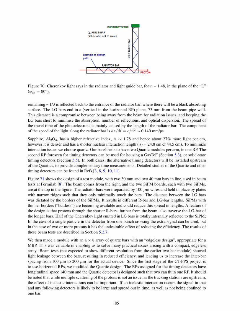
Figure 70: Cherenkov light rays in the radiator and light guide bar, for n = 1.48, in the plane of the “L”(φch = 90).

remaining∼1/3 is reflected back to the entrance of the radiator bar, where there will be a black absorbingsurface. The LG bars end in a (vertical in the horizontal RP) plane, 73 mm from the beam pipe wall.This distance is a compromise between being away from the beam for radiation issues, and keeping theLG bars short to minimise the absorption, number of reflections, and optical dispersion. The spread ofthe travel time of the photoelectrons is mainly caused by the length of the radiator bar. The componentof the speed of the light along the radiator bar is dz/dt = c/n2 ∼ 0.140 mm/ps.

Sapphire, Al2O3, has a higher refractive index, n ∼ 1.78 and hence about 27% more light per cm,however it is denser and has a shorter nuclear interaction length (λI = 24.8 cm cf 44.5 cm). To minimizeinteraction issues we choose quartz. Our baseline is to have two Quartic modules per arm, in one RP. Thesecond RP foreseen for timing detectors can be used for housing a GasToF (Section 5.3), or solid-statetiming detectors (Section 5.5). In both cases, the alternative timing detectors will be installed upstreamof the Quartics, to provide complementary time measurements. Detailed studies of the Quartic and othertiming detectors can be found in Refs.[3, 8, 9, 10, 11].

Figure 71 shows the design of a test module, with two 30 mm and two 40 mm bars in line, used in beamtests at Fermilab [8]. The beam comes from the right, and the two SiPM boards, each with two SiPMs,are at the top in the figure. The radiator bars were separated by 100 µm wires and held in place by plateswith narrow ridges such that they only minimally touch the bars. The distance between the LG barswas dictated by the borders of the SiPMs. It results in different R-bar and LG-bar lengths. SiPMs withthinner borders (“buttless”) are becoming available and could reduce this spread in lengths. A feature ofthe design is that protons through the shorter R-bars, farther from the beam, also traverse the LG-bar ofthe longer bars. Half of the Cherenkov light emitted in LG bars is totally internally reflected to the SiPM;In the case of a single particle in the detector from one bunch crossing the extra signal can be used, butin the case of two or more protons it has the undesirable effect of reducing the efficiency. The results ofthese beam tests are described in Section 5.2.7.

We then made a module with an 4 × 5 array of quartz bars with an “edgeless design”, appropriate for aMBP. This was valuable in enabling us to solve many practical issues arising with a compact, edgelessarray. Beam tests (not expected to show different resolution from the earlier two-bar module) showedlight leakage between the bars, resulting in reduced efficiency, and leading us to increase the inter-barspacing from 100 µm to 200 µm for the actual device. Since the first stage of the CT-PPS project isto use horizontal RPs, we modified the Quartic design. The RPs assigned for the timing detectors havelongitudinal space 140 mm and the Quartic detector is designed such that two can fit in one RP. It shouldbe noted that while multiple scattering of the protons is not an issue, as the tracking stations are upstream,the effect of inelastic interactions can be important. If an inelastic interaction occurs the signal in thatand any following detectors is likely to be large and spread out in time, as well as not being confined toone bar.

85

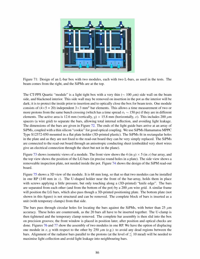
Figure 71: Design of an L-bar box with two modules, each with two L-bars, as used in the tests. Thebeam comes from the right, and the SiPMs are at the top.

The CT-PPS Quartic “module” is a light tight box with a very thin (∼ 100 µm) side wall on the beamside, and blackened interior. This side wall may be removed on insertion in the pot as the interior will bedark; it is to protect the inside prior to insertion and to optically close the box for beam tests. One moduleconsists of (4×5 = 20) independent 3×3 mm2 bar elements. This allows a time measurement of two ormore protons from the same bunch crossing (which has a time spread σt ∼ 150 ps) if they are in differentelements. The active area is 12.6 mm (vertically, y) × 15.8 mm (horizontally, x). This includes 200 µmspacers (a wire grid) to separate the bars, allowing total internal reflection, and avoiding light leakage.The dimensions of the bars are given in Figure 72. The ends of the light guide bars arrive at an array ofSiPMs, coupled with a thin silicon “cookie” for good optical coupling. We use SiPMs Hamamatsu MPPCType S12572-050 mounted in a flat plate holder (3D-printed plastic). The SiPMs fit in rectangular holesin the plate and as they are not fixed to the read-out board they can be very simply replaced. The SiPMsare connected to the read-out board through an anisotropic conducting sheet (embedded very short wiresgive an electrical connection through the sheet but not in the plane).

Figure 73 shows isometric views of a module. The front view shows the 4 (in y)× 5 (in x) bar array, andthe top view shows the position of the LG bars (in precise round holes in a plate). The side view shows aremoveable inspection plate, not needed inside the pot. Figure 74 shows the design of the SiPM read-outboard.

Figure 75 shows a 3D view of the module. It is 68 mm long, so that so that two modules can be installedin one RP (140 mm in z). The U-shaped holder near the front of the bar-array, holds them in placewith screws applying a little pressure, but only touching along a (3D-printed) “knife edge”. The barsare separated from each other (and from the bottom of the pot) by a 200 µm wire grid. A similar framewill position the LG bars, which also pass though a 3D-printed positioning plate. The bottom plate (notshown in this figure) is not structural and can be removed. The complete block of bars is inserted as aunit (with temporary clamps) from that side.

The bars pass through circular holes for locating the bars against the SiPMs, with better than 25 µmaccuracy. These holes are countersunk, as the 20 bars all have to be inserted together. The U-clamp isthen tightened and the temporary clamp removed. The complete bar assembly is then slid into the boxon precision grooves; the front window is placed in position later, after position and optical checks aredone. Figures 76 and 77 show the assembly of two modules in one RP. We have the option of displacingone module in x, y with respect to the other by 250 µm (e.g.) to avoid any dead regions between thebars. Alignment of the radiator bars parallel to the protons (at the level of . 10 mrad) will be needed tomaximise light collection and avoid light leakage into neighbouring bars.

86

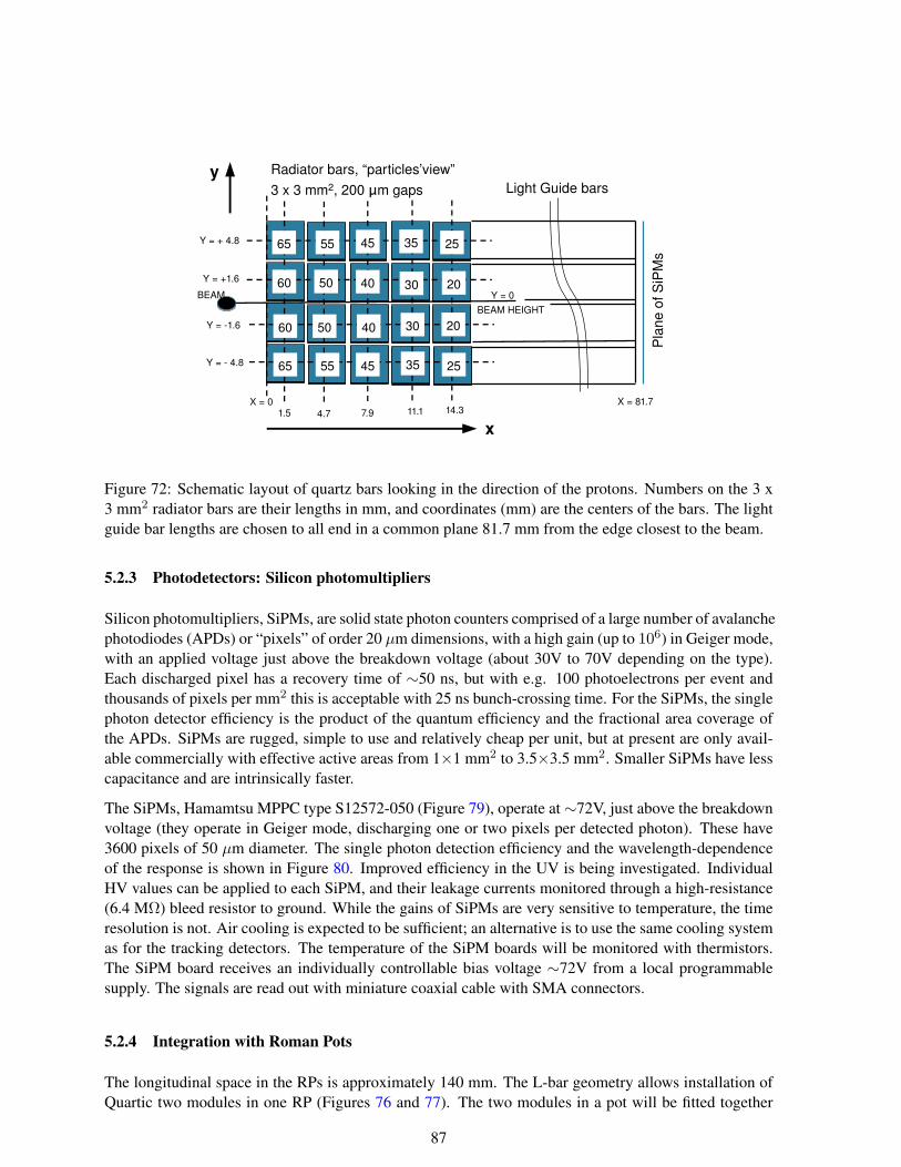
Y = 0BEAM HEIGHT

Y = +1.6

Y = 1.6

Y = 4.8

Y = + 4.8

BEAM

1.5 4.7 7.9 11.1 14.3

60

60

65

65

50

50

55

55

45

45

40

40

35

35

30

30

25

25

20

20

Radiator bars, “particles’view”3 x 3 mm2, 200 m gapsμ

X = 81.7X = 0

Light Guide bars

Plan

e of

SiP

Ms

y

x

Figure 72: Schematic layout of quartz bars looking in the direction of the protons. Numbers on the 3 x3 mm2 radiator bars are their lengths in mm, and coordinates (mm) are the centers of the bars. The lightguide bar lengths are chosen to all end in a common plane 81.7 mm from the edge closest to the beam.

5.2.3 Photodetectors: Silicon photomultipliers

Silicon photomultipliers, SiPMs, are solid state photon counters comprised of a large number of avalanchephotodiodes (APDs) or “pixels” of order 20 µm dimensions, with a high gain (up to 106) in Geiger mode,with an applied voltage just above the breakdown voltage (about 30V to 70V depending on the type).Each discharged pixel has a recovery time of ∼50 ns, but with e.g. 100 photoelectrons per event andthousands of pixels per mm2 this is acceptable with 25 ns bunch-crossing time. For the SiPMs, the singlephoton detector efficiency is the product of the quantum efficiency and the fractional area coverage ofthe APDs. SiPMs are rugged, simple to use and relatively cheap per unit, but at present are only avail-able commercially with effective active areas from 1×1 mm2 to 3.5×3.5 mm2. Smaller SiPMs have lesscapacitance and are intrinsically faster.

The SiPMs, Hamamtsu MPPC type S12572-050 (Figure 79), operate at∼72V, just above the breakdownvoltage (they operate in Geiger mode, discharging one or two pixels per detected photon). These have3600 pixels of 50 µm diameter. The single photon detection efficiency and the wavelength-dependenceof the response is shown in Figure 80. Improved efficiency in the UV is being investigated. IndividualHV values can be applied to each SiPM, and their leakage currents monitored through a high-resistance(6.4 MΩ) bleed resistor to ground. While the gains of SiPMs are very sensitive to temperature, the timeresolution is not. Air cooling is expected to be sufficient; an alternative is to use the same cooling systemas for the tracking detectors. The temperature of the SiPM boards will be monitored with thermistors.The SiPM board receives an individually controllable bias voltage ∼72V from a local programmablesupply. The signals are read out with miniature coaxial cable with SMA connectors.

5.2.4 Integration with Roman Pots

The longitudinal space in the RPs is approximately 140 mm. The L-bar geometry allows installation ofQuartic two modules in one RP (Figures 76 and 77). The two modules in a pot will be fitted together

87

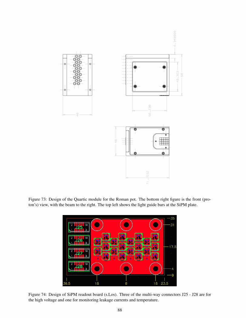
Figure 73: Design of the Quartic module for the Roman pot. The bottom right figure is the front (pro-ton’s) view, with the beam to the right. The top left shows the light guide bars at the SiPM plate.

Figure 74: Design of SiPM readout board (s.Los). Three of the multi-way connectors J25 - J28 are forthe high voltage and one for monitoring leakage currents and temperature.

88

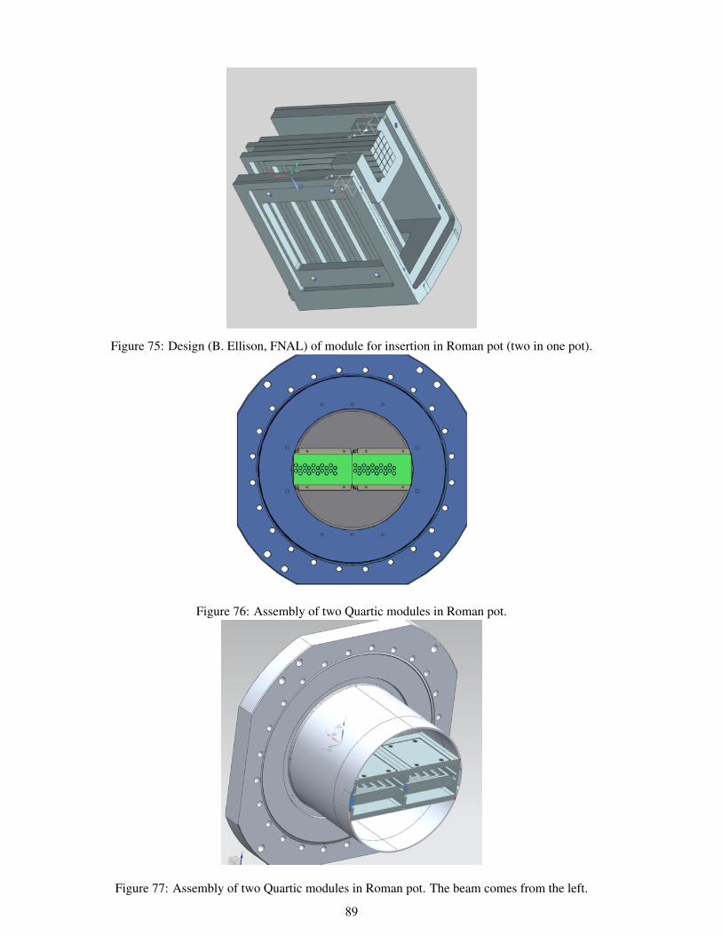
Figure 75: Design (B. Ellison, FNAL) of module for insertion in Roman pot (two in one pot).

Figure 76: Assembly of two Quartic modules in Roman pot.

Figure 77: Assembly of two Quartic modules in Roman pot. The beam comes from the left.

89

Figure 78: “Particle eye view” of bar array in pot. This is a modified design (D.Druzhkin) reducing thematerial close to the beam.

precisely using dowel pins.

Figures 73 and 75 show the design of the module for insertion into the horizontal RP. A slightly modifiedversion (Figure 78) reduces the material close to the beam. The protons enter through a thin window(nominally 100 µm aluminium, but it has no mechanical purpose, it is for absorption of reflected lightand light exclusion). The array of radiator bars is clamped on the three sides away from the beam with aplastic U-clamp, touching each bar only along a fine line. For assembly of the bar array a 4-sided clampis placed temporarily around the front of the array. The SiPM plate and read-out board are preciselypositioned by dowels with respect to the L-bar positioning plate.

5.2.5 Monitoring, alignment, and in situ calibration

The rates in each bar are monitored both online and offline. The rates are expected to be up-downsymmetric about the beam height (as can also be determined from the tracker), column-by-column. Thisgives a measure of the centre of the beam in y, assuming the backgrounds are relatively small. For agiven row in y the rates will fall with x with two components: protons from collisions and beam halobackground. The former will be compared with predicted t-distributions, and it is valuable to measurethe latter. When the RPs are inserted at the beginning of stores the rates will be carefully monitored, e.g.partially withdrawing in the event of an abnormal increase.

Initial relative alignment of the Quartic bars and tracker will be achieved by matching the individual baredges in x and y with the track distributions.

A pair of light-emitting diodes will be mounted inside the module in such a way that some light iscaptured in each bar. This will be pulsed when there is no beam as a control of all the SiPMs and theirreadout.

Occupancy of the bars will be monitored in real time, as functions of the instantaneous luminosity andbackground conditions. Geometrical matching between the bar array and the trackers will also be mea-sured; the 200 µm gaps between the bars can also provide a check.

A calibration of the absolute time difference between the protons, ∆tpp, can be derived by matchingzpp = zX using real events of the type p+ p→ p+X + p, where X is a set of particles measured in thecentral detector. After kinematic matching of X to the protons (four-momentum conservation) the 2Dplot of zpp vs zX will show a ridge which calibrates both zpp = 0 as well as checking the time scale.

While the time difference between the “left” and “right” protons, tL − tR, gives zpp, the time sum, or(tL + tR)/2 (minus a constant), would provide another, orthogonal, variable for pileup rejection if the

90

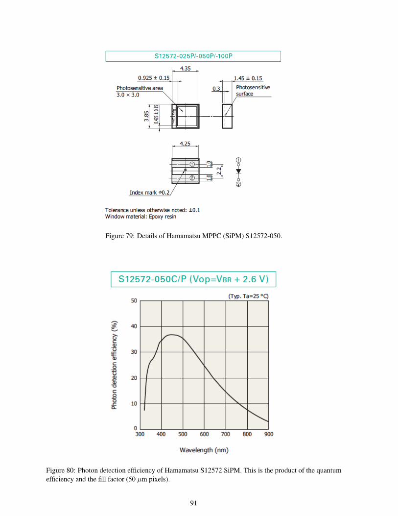
Figure 79: Details of Hamamatsu MPPC (SiPM) S12572-050.

Figure 80: Photon detection efficiency of Hamamatsu S12572 SiPM. This is the product of the quantumefficiency and the fill factor (50 µm pixels).

91

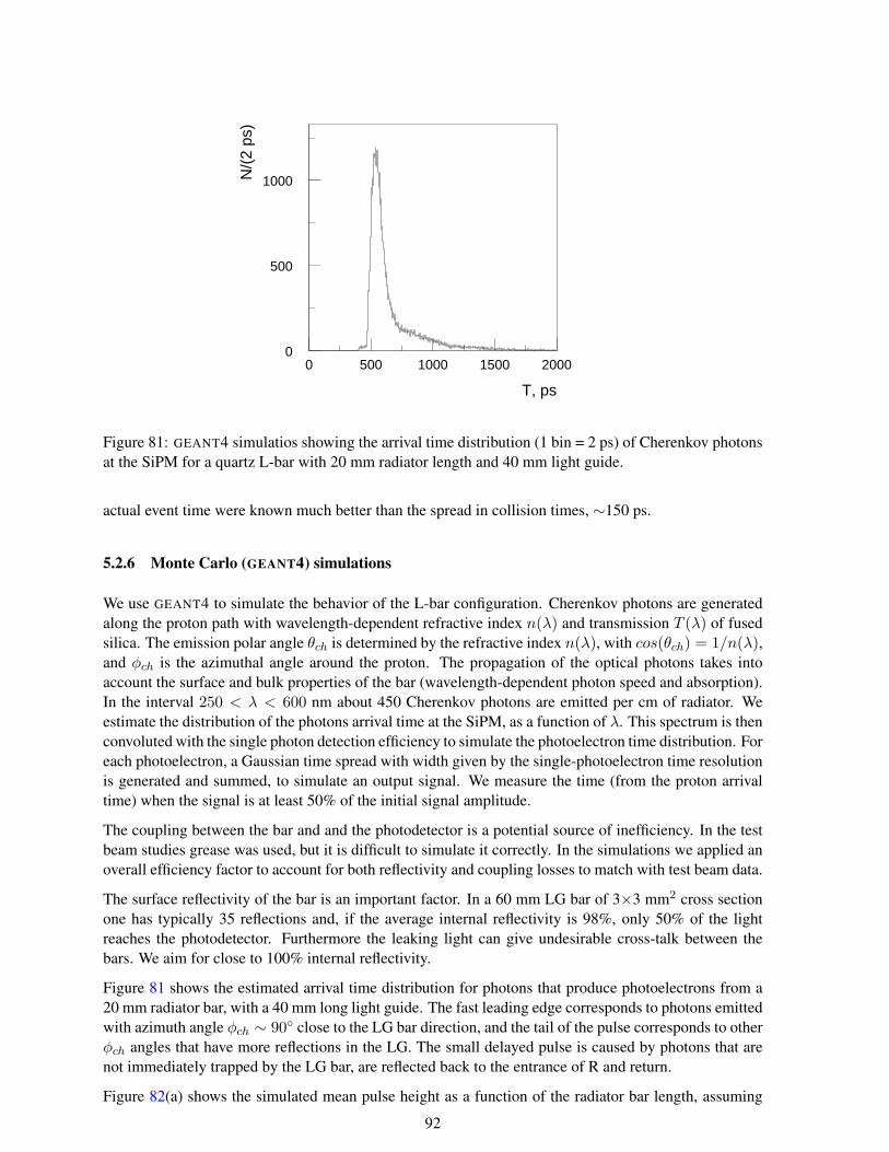
0

500

1000

0 500 1000 1500 2000

T, ps

N/(

2 ps

)

Figure 81: GEANT4 simulatios showing the arrival time distribution (1 bin = 2 ps) of Cherenkov photonsat the SiPM for a quartz L-bar with 20 mm radiator length and 40 mm light guide.

actual event time were known much better than the spread in collision times, ∼150 ps.

5.2.6 Monte Carlo (GEANT4) simulations

We use GEANT4 to simulate the behavior of the L-bar configuration. Cherenkov photons are generatedalong the proton path with wavelength-dependent refractive index n(λ) and transmission T (λ) of fusedsilica. The emission polar angle θch is determined by the refractive index n(λ), with cos(θch) = 1/n(λ),and φch is the azimuthal angle around the proton. The propagation of the optical photons takes intoaccount the surface and bulk properties of the bar (wavelength-dependent photon speed and absorption).In the interval 250 < λ < 600 nm about 450 Cherenkov photons are emitted per cm of radiator. Weestimate the distribution of the photons arrival time at the SiPM, as a function of λ. This spectrum is thenconvoluted with the single photon detection efficiency to simulate the photoelectron time distribution. Foreach photoelectron, a Gaussian time spread with width given by the single-photoelectron time resolutionis generated and summed, to simulate an output signal. We measure the time (from the proton arrivaltime) when the signal is at least 50% of the initial signal amplitude.

The coupling between the bar and and the photodetector is a potential source of inefficiency. In the testbeam studies grease was used, but it is difficult to simulate it correctly. In the simulations we applied anoverall efficiency factor to account for both reflectivity and coupling losses to match with test beam data.

The surface reflectivity of the bar is an important factor. In a 60 mm LG bar of 3×3 mm2 cross sectionone has typically 35 reflections and, if the average internal reflectivity is 98%, only 50% of the lightreaches the photodetector. Furthermore the leaking light can give undesirable cross-talk between thebars. We aim for close to 100% internal reflectivity.

Figure 81 shows the estimated arrival time distribution for photons that produce photoelectrons from a20 mm radiator bar, with a 40 mm long light guide. The fast leading edge corresponds to photons emittedwith azimuth angle φch ∼ 90 close to the LG bar direction, and the tail of the pulse corresponds to otherφch angles that have more reflections in the LG. The small delayed pulse is caused by photons that arenot immediately trapped by the LG bar, are reflected back to the entrance of R and return.

Figure 82(a) shows the simulated mean pulse height as a function of the radiator bar length, assuming

92

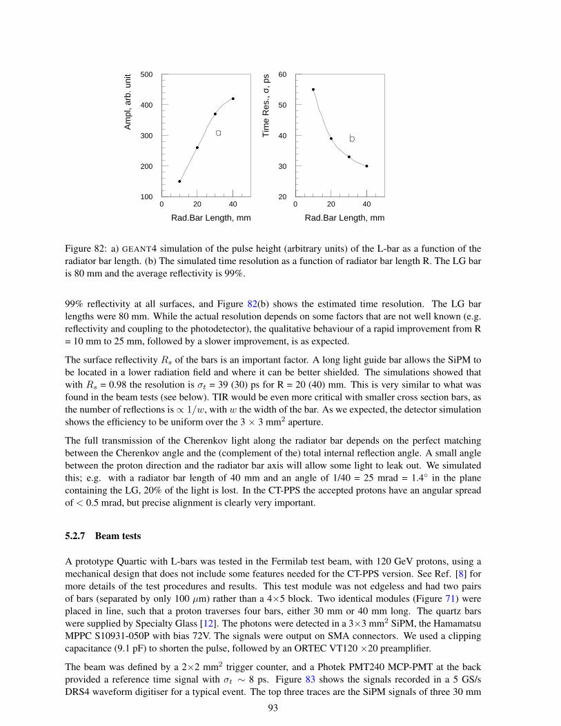
100

200

300

400

500

0 20 40

Rad.Bar Length, mm

Am

pl, a

rb. u

nit

20

30

40

50

60

0 20 40

Rad.Bar Length, mm

Tim

e R

es.,

σ, p

s

Figure 82: a) GEANT4 simulation of the pulse height (arbitrary units) of the L-bar as a function of theradiator bar length. (b) The simulated time resolution as a function of radiator bar length R. The LG baris 80 mm and the average reflectivity is 99%.

99% reflectivity at all surfaces, and Figure 82(b) shows the estimated time resolution. The LG barlengths were 80 mm. While the actual resolution depends on some factors that are not well known (e.g.reflectivity and coupling to the photodetector), the qualitative behaviour of a rapid improvement from R= 10 mm to 25 mm, followed by a slower improvement, is as expected.

The surface reflectivity Rs of the bars is an important factor. A long light guide bar allows the SiPM tobe located in a lower radiation field and where it can be better shielded. The simulations showed thatwith Rs = 0.98 the resolution is σt = 39 (30) ps for R = 20 (40) mm. This is very similar to what wasfound in the beam tests (see below). TIR would be even more critical with smaller cross section bars, asthe number of reflections is ∝ 1/w, with w the width of the bar. As we expected, the detector simulationshows the efficiency to be uniform over the 3 × 3 mm2 aperture.

The full transmission of the Cherenkov light along the radiator bar depends on the perfect matchingbetween the Cherenkov angle and the (complement of the) total internal reflection angle. A small anglebetween the proton direction and the radiator bar axis will allow some light to leak out. We simulatedthis; e.g. with a radiator bar length of 40 mm and an angle of 1/40 = 25 mrad = 1.4 in the planecontaining the LG, 20% of the light is lost. In the CT-PPS the accepted protons have an angular spreadof < 0.5 mrad, but precise alignment is clearly very important.

5.2.7 Beam tests

A prototype Quartic with L-bars was tested in the Fermilab test beam, with 120 GeV protons, using amechanical design that does not include some features needed for the CT-PPS version. See Ref. [8] formore details of the test procedures and results. This test module was not edgeless and had two pairsof bars (separated by only 100 µm) rather than a 4×5 block. Two identical modules (Figure 71) wereplaced in line, such that a proton traverses four bars, either 30 mm or 40 mm long. The quartz barswere supplied by Specialty Glass [12]. The photons were detected in a 3×3 mm2 SiPM, the HamamatsuMPPC S10931-050P with bias 72V. The signals were output on SMA connectors. We used a clippingcapacitance (9.1 pF) to shorten the pulse, followed by an ORTEC VT120 ×20 preamplifier.

The beam was defined by a 2×2 mm2 trigger counter, and a Photek PMT240 MCP-PMT at the backprovided a reference time signal with σt ∼ 8 ps. Figure 83 shows the signals recorded in a 5 GS/sDRS4 waveform digitiser for a typical event. The top three traces are the SiPM signals of three 30 mm

93

Figure 83: Waveforms in the DRS-4 of one proton through three L-bars and the PMT240 (bottom trace).The time scale is 2 ns/div and the vertical scale 20 mV/div for the top three traces (SiPM’s) and 50mV/div for the bottom trace (reference PMT240).

Figure 84: Pulse height distribution in a 40 mm radiator bar. The overflow is due to interactions.

Cherenkov bars, 20 mV/div, 2 ns/div (200 ps per sample), joined by straight-line segments, and thebottom trace (50 mV/div) is the PMT240 reference signal. Typical pulse heights are about 80 mV withan 800 ps risetime. Figure 84 shows the pulse-height distribution for one bar, consistent with Npe ∼ 50.The entries in the overflow bin are due to interactions, upstream or in the bar. Good timing measurementswere obtained by a linear fit to the two points before and after the 50% of pulse maximum amplitude,finding the time at which that line crossed the 50% level, and then applying a time-slewing correction.More complete waveform fits were found to be not significantly better.

From the spread in signal amplitudes we estimated that the number of photoelectrons isNpe ∼ 80−100.Figure 85 shows, after applying pulse height-slewing corrections, the time difference between one barand the reference time signal, with a time resolution of σ = 35.3 ps. After unfolding the electronics andreference time resolutions, the time resolution of the 30 mm bars was ∼ 33 ps. Alternatively, withoutusing the PMT240 reference time but comparing the different bar times we found σt = 31 ps. We plan tohave two modules in-line in one pot, which are expected to give a time resolution of 21 ps.

After these corrections, the time differences between the four short bars and the reference PMT240 signalhad widths, from Gaussian fits, σt = 35 - 40 ps, with 〈σt〉 = 37.5 ps. Figure 85 shows one example, withσ(∆t) = 34.9 ps, showing no background or inefficiency. The single-photon time resolution of the SiPM

94

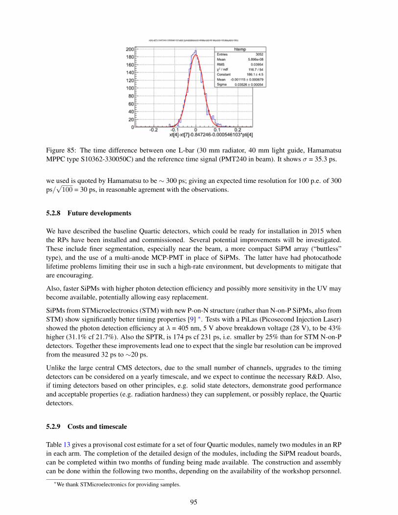
Figure 85: The time difference between one L-bar (30 mm radiator, 40 mm light guide, HamamatsuMPPC type S10362-330050C) and the reference time signal (PMT240 in beam). It shows σ = 35.3 ps.

we used is quoted by Hamamatsu to be ∼ 300 ps; giving an expected time resolution for 100 p.e. of 300ps/√

100 = 30 ps, in reasonable agrement with the observations.

5.2.8 Future developments

We have described the baseline Quartic detectors, which could be ready for installation in 2015 whenthe RPs have been installed and commissioned. Several potential improvements will be investigated.These include finer segmentation, especially near the beam, a more compact SiPM array (“buttless”type), and the use of a multi-anode MCP-PMT in place of SiPMs. The latter have had photocathodelifetime problems limiting their use in such a high-rate environment, but developments to mitigate thatare encouraging.

Also, faster SiPMs with higher photon detection efficiency and possibly more sensitivity in the UV maybecome available, potentially allowing easy replacement.

SiPMs from STMicroelectronics (STM) with new P-on-N structure (rather than N-on-P SiPMs, also fromSTM) show significantly better timing properties [9] ∗. Tests with a PiLas (Picosecond Injection Laser)showed the photon detection efficiency at λ = 405 nm, 5 V above breakdown voltage (28 V), to be 43%higher (31.1% cf 21.7%). Also the SPTR, is 174 ps cf 231 ps, i.e. smaller by 25% than for STM N-on-Pdetectors. Together these improvements lead one to expect that the single bar resolution can be improvedfrom the measured 32 ps to ∼20 ps.

Unlike the large central CMS detectors, due to the small number of channels, upgrades to the timingdetectors can be considered on a yearly timescale, and we expect to continue the necessary R&D. Also,if timing detectors based on other principles, e.g. solid state detectors, demonstrate good performanceand acceptable properties (e.g. radiation hardness) they can supplement, or possibly replace, the Quarticdetectors.

5.2.9 Costs and timescale

Table 13 gives a provisonal cost estimate for a set of four Quartic modules, namely two modules in an RPin each arm. The completion of the detailed design of the modules, including the SiPM readout boards,can be completed within two months of funding being made available. The construction and assemblycan be done within the following two months, depending on the availability of the workshop personnel.

∗We thank STMicroelectronics for providing samples.

95

Item unit Number Unit price Total Comment

(US$) (US K$)

Quartz bars bar 20×4 = 80 350 28 Specialty Glass

MPPC/SiPMs (20)/module 80 80 6.4 e.g. Hamamatsu

Other components module 4 250 1.0

Total modules 35.4

Low voltage Station 2 600 1.2

Current monitor Central 1 2500 2.5

Temp. Monitor station 2 1000 2.0

Cables (CERN)

Shipping <1

Board design person-weeks 3 4K 12 Fermi design office

Mechanical design person-weeks 3 4 K 12 Fermi design office

Assembly person weeks 4 4 K 16 Fermi workshops

Table 13: Provisional costs for a pair of Quartic modules, each of 20 bars, in each arm, not includingDAQ. Design and Assembly costs reduce by ∼ ×0.5 if done outside Fermilab.

The timescale for making the quartz bars is about 8 weeks from receipt of order. The bar assembly canbe installed last in the module. If funds are provided very soon, it should be possible to deliver the fourmodules to CERN by the end of 2014.

5.2.10 Summary of Quartic detectors

The L-bar Quartic design satisfies the requirements of edgelessness (within about 100 µm), sufficientradiation hardness, ability to measure several protons within a bunch crossing (time spread σ = 150ps) if in separate bars, and to be active every 25 ns (the bunch separation). We plan to construct andinstall a pair of L-bar Quartic modules, with SiPM photodetectors, in a RP on each arm, and use themin 2015 to assess their performance in realistic conditions, as well as for physics in the low pileup runs.The modules will be constructed at Fermilab and the signals from the SiPM board sent to a local DAQ(which will be the responsibity of the Lisbon Group).

Further development will continue to improve their time resolution and possibly the spatial segmentation.Therefore R&D will continue, and improved versions could be ready for installation at the end of 2015.

5.3 Gas Cherenkov detector

GasToF is a gas Cherenkov detector with direct detection of the very forward light cone, without useof internal reflections. It is intrinsically very fast, providing excellent time resolution, even with singlephotons. Since in its standard configuration the Cherenkov light is simply reflected by a thin, flat 45

mirror onto a photocathode of a Micro Channel Plate photomultiplier (MCP-PMT), its optics is trivialthanks to the small chromatic dispersion and the very small Cherenkov angle in gases. This also makes it

96

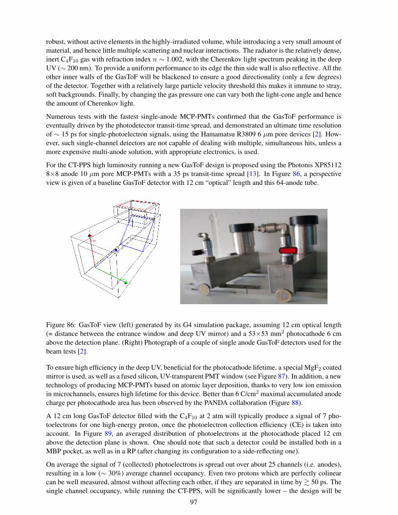
robust, without active elements in the highly-irradiated volume, while introducing a very small amount ofmaterial, and hence little multiple scattering and nuclear interactions. The radiator is the relatively dense,inert C4F10 gas with refraction index n ∼ 1.002, with the Cherenkov light spectrum peaking in the deepUV (∼ 200 nm). To provide a uniform performance to its edge the thin side wall is also reflective. All theother inner walls of the GasToF will be blackened to ensure a good directionality (only a few degrees)of the detector. Together with a relatively large particle velocity threshold this makes it immune to stray,soft backgrounds. Finally, by changing the gas pressure one can vary both the light-cone angle and hencethe amount of Cherenkov light.

Numerous tests with the fastest single-anode MCP-PMTs confirmed that the GasToF performance iseventually driven by the photodetector transit-time spread, and demonstrated an ultimate time resolutionof ∼ 15 ps for single-photoelectron signals, using the Hamamatsu R3809 6 µm pore devices [2]. How-ever, such single-channel detectors are not capable of dealing with multiple, simultaneous hits, unless amore expensive multi-anode solution, with appropriate electronics, is used.

For the CT-PPS high luminosity running a new GasToF design is proposed using the Photonis XP851128×8 anode 10 µm pore MCP-PMTs with a 35 ps transit-time spread [13]. In Figure 86, a perspectiveview is given of a baseline GasToF detector with 12 cm “optical” length and this 64-anode tube.

Figure 86: GasToF view (left) generated by its G4 simulation package, assuming 12 cm optical length(= distance between the entrance window and deep UV mirror) and a 53×53 mm2 photocathode 6 cmabove the detection plane. (Right) Photograph of a couple of single anode GasToF detectors used for thebeam tests [2].

To ensure high efficiency in the deep UV, beneficial for the photocathode lifetime, a special MgF2 coatedmirror is used, as well as a fused silicon, UV-transparent PMT window (see Figure 87). In addition, a newtechnology of producing MCP-PMTs based on atomic layer deposition, thanks to very low ion emissionin microchannels, ensures high lifetime for this device. Better than 6 C/cm2 maximal accumulated anodecharge per photocathode area has been observed by the PANDA collaboration (Figure 88).

A 12 cm long GasToF detector filled with the C4F10 at 2 atm will typically produce a signal of 7 pho-toelectrons for one high-energy proton, once the photoelectron collection efficiency (CE) is taken intoaccount. In Figure 89, an averaged distribution of photoelectrons at the photocathode placed 12 cmabove the detection plane is shown. One should note that such a detector could be installed both in aMBP pocket, as well as in a RP (after changing its configuration to a side-reflecting one).

On average the signal of 7 (collected) photoelectrons is spread out over about 25 channels (i.e. anodes),resulting in a low (∼ 30%) average channel occupancy. Even two protons which are perfectly colinearcan be well measured, almost without affecting each other, if they are separated in time by & 50 ps. Thesingle channel occupancy, while running the CT-PPS, will be significantly lower – the design will be

97

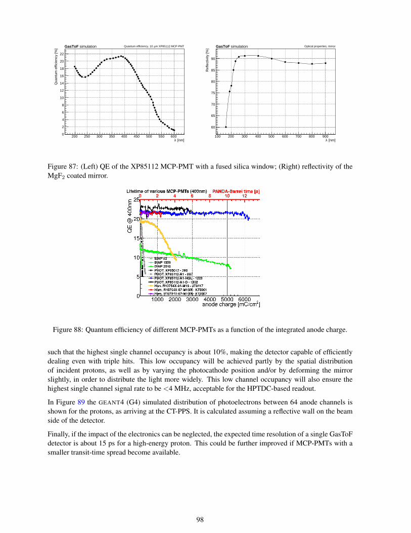
[nm]λ200 250 300 350 400 450 500 550 600

Qua

ntum

effi

cien

cy [%

]

0

2

4

6

8

10

12

14

16

18

20

22

GasToF simulation m XP85112 MCP-PMTµQuantum efficiency, 10

[nm]λ100 200 300 400 500 600 700 800 900

Ref

lect

ivity

[%]

60

65

70

75

80

85

90

GasToF simulation Optical properties, mirror

Figure 87: (Left) QE of the XP85112 MCP-PMT with a fused silica window; (Right) reflectivity of theMgF2 coated mirror.

Figure 88: Quantum efficiency of different MCP-PMTs as a function of the integrated anode charge.

such that the highest single channel occupancy is about 10%, making the detector capable of efficientlydealing even with triple hits. This low occupancy will be achieved partly by the spatial distributionof incident protons, as well as by varying the photocathode position and/or by deforming the mirrorslightly, in order to distribute the light more widely. This low channel occupancy will also ensure thehighest single channel signal rate to be <4 MHz, acceptable for the HPTDC-based readout.

In Figure 89 the GEANT4 (G4) simulated distribution of photoelectrons between 64 anode channels isshown for the protons, as arriving at the CT-PPS. It is calculated assuming a reflective wall on the beamside of the detector.

Finally, if the impact of the electronics can be neglected, the expected time resolution of a single GasToFdetector is about 15 ps for a high-energy proton. This could be further improved if MCP-PMTs with asmaller transit-time spread become available.

98

y [cm]-2 -1 0 1 2

z [c

m]

-2

-1

0

1

2

0

0.001

0.002

0.003

0.004

0.005

0.006

0.007

0.008

0.009

GasToF simulation = 6.5 TeVp

12 cm horiz.+vert. opt. length, 2 atm, photoelec., E

y [cm]-3 -2 -1 0 1 2 3

z [c

m]

-3

-2

-1

0

1

2

3

0

0.2

0.4

0.6

0.8

1

1.2

1.4GasToF simulation = 6.5 TeV

p12 cm horiz.+vert. opt. length, 2 atm, photoelec., E

Figure 89: Example of the GasToF performance for a 12 cm detector with the gas at 2 atm, and assumingcentral, on-axis 6.5 TeV protons.The G4 distributions of photoelectrons (without CE) at a photocathodedisplaced by 12 cm, where the right plot give the average number photoelectrons ’per anode’.

y [cm]-3 -2 -1 0 1 2 3

z [c

m]

-3

-2

-1

0

1

2

3

0

0.2

0.4

0.6

0.8

1

1.2

1.4

1.6

1.8

GasToF simulation = 6.5 TeVp

12 cm horiz.+vert. opt. length, 2 atm, photoelec., E

Figure 90: Example of the GasToF performance for a 12+12 cm detector (with the gas at 2 atm) forprotons reaching the PPS. The G4 distribution of photoelectrons among the MCP-PMT 64 channels forminimum bias protons tracked trough the LHC beam line, assuming µ = 50 - each bin represents anaverage number of photoelectrons (without CE) per beam collision.

99

5.4 Readout System of the Cherenkov Detectors

5.4.1 Requirements

The task of the readout system is to provide time and amplitude measurements of the pulses generatedby the photosensors associated to the Cherenkov detectors, and to transmit the digitized data to the dataacquisition system. Given the similar characteristics of the Quartic and Gastof detectors, the readoutsystem is expected to be suitable for both detectors.

The Cherenkov timing detectors are composed of a number of modules installed in one or more RP (orMBP). The readout system follows the same modularity, and is composed of independent units (readoutmodule) interfacing to the CT-PPS DAQ/Trigger system. Each readout module has 64 channels suitablefor use with the baseline Quartic module (20 channels), but also with possible Quartic modules with finergranularity and with the Gastof 8× 8 anode MCP-PMT.

Each electronic channel must be able to handle very fast pulses (rise time ∼ 1 ns) from silicon photo-multipliers or micro-channel plates. The photon yield of the Cherenkov signals per channel range from1 photon in the case of Gastof MCP to about 100 photons in the case of Quartic. The SiPM gain is of theorder of 106 while the MCP-PMT will be operated at about 10 times lower gain to limit the total chargecollected (see Section 5.3). Therefore the dynamic range of the input signals is in the range of 20 fC to20 pC.

The timing precision of the readout system is required to be 20 ps, which, combined with a similarprecision of the Quartic detector, would yield 30 ps precision per module, and global precision (twomodules) of about 20 ps. When associated to one Gastof detector, assuming 7 photoelectrons per protonand a precision of 30 ps per MCP-PMT channel, we may estimate that the readout system would providea measurement with 15 ps precision.

The readout system is also required to provide the measurement of the input pulse amplitude. Whilethis measurement is not directly used in the reconstruction of the collision vertex, the knowledge of theamplitude is mandatory for detector calibration, time corrections (e.g. “time-walk”) and pulse pile-uprejection.

The readout system is required to have double hit resolution better than 25 ns, suitable for operation with25 ns bunch separation without loss of efficiency, and to sustain a maximum rate of 6 MHz per channel,corresponding to a maximum channel occupancy of 20% at 25 ns LHC beam operation, averaged overall channels. While the average occupancy of the Quartic channels (3 × 3 mm2 quartz bars) is 20% foraverage pile-up of 50 events, the highly non-uniform occupancy of the detector (the occupancy of theinnermost channels reach 70%) induces a significant readout inefficiency for a number of pile-up eventslarger than 25. To sustain twice this value, as foreseen in Run2, a fine-granularity Quartic version willbe required. In the case of the Gastof detector, a channel occupancy smaller than 20% is expected (seeSection 5.3).

The readout system is required to provide on-detector L1 trigger matching, allowing extraction of thedetector data in a time window around the L1 time, local event building and data transmission to theDAQ system. The data rate of a readout module, assuming readout of 10 channels after zero suppression,3 bunch crossings time window, 32 bit event data per channel, and 100 kHz L1 rate, is estimated to be100 Mb/s.

The timing detector readout system is expected to provide hit information and time measurement at thebunch crossing rate to be used by the trigger system. By combining the information from the two PPSarms, the L1 can estimate the z-vertex coordinate, allowing to select events in the tails of the z-vertexdistribution where the pileup density is smaller. This capability would provide a reduction of the L1 rateof high cross-section processes so that it fits within the L1 rate constraints, selecting at the same time theevents less affected by pileup. The trigger requirement implies the use of a low latency TDC delivering

100

Figure 91: Time resolution of laser pulses as a function of the number of photo-electrons measured withMPPC and the NINO-HPTDC electronics chain.

conversion data at the bunch crossing rate.

In order to achieve the desired time resolution, the front-end timing electronics must be located in theRPs or a nearby region (1-2 m distance). This raises issues of radiation tolerance since the radiationlevels in the RPs, in the region 200 m from IP, are expected to be 100 Gray and 1012 neq/cm2 for100 fb−1 of integrated luminosity. Together with machine experts, we have explored the feasibility ofdigging a hole in the tunnel floor concrete below the timing RPs, which would provide a substantialreduction of the radiation exposure. While this possibility is technically feasible, the proposal could notbe accommodated in the present LHC LS1 schedule but would be possible if necessary in the wintertechnical stop 2015-16.

5.4.2 System design

The main guideline in the design of the timing detector readout system was to reuse well known compo-nents with adequate performance, allowing to streamline the design and implementation of the systemso that it may be possible to evaluate the timing detectors in the LHC beam in 2015.

We have therefore decided to base our system on the amplifier-discriminator NINO and the time-to-digital converter HPTDC. Both chips have been developed by CERN’s microelectronics group for theLHC experiments. The HPTDC chip is used in the CMS muon system, while the NINO and HPTDCchips are associated in the time-of-flight detector of the ALICE experiment. These chips are now widelyused in many applications, including PET Time-of-Flight.

The EndoTOFPET-US collaboration † has studied the time resolution of the NINO-HPTDC readoutchain, using laser pulses detected by 3 × 3 mm2 SiPMs (Hamamatsu MPPC) with SPAD size of 50µm[14]. The measured time resolution as a function of the number of photo-electrons is shown in Figure 91.For 100 photoelectrons a resolution better than 20 ps is achieved.

The NINO amplifier-discriminator is implemented in a 8 channel ASIC. A newer version with 32 chan-nels developed by an external group is also suitable. The time binning and number of channels of theHPTDC ASIC is configurable. In our case we use the HPTDC high-resolution mode, which provides 8channels with 25 ps time binning. The timing readout system is designed to be integrated in the com-mon CT-PPS DAQ and Control system, based on the CMS Pixel FED and FEC boards. The FED board

†This project have been funded by the European Union 7th Framework Program (FP7/ 2007-2013) under Grant AgreementNo. 256984 (EndoTOFPET-US)

101

Detector

Bias V

Monit. Laser

T, I slow control

NINO Ampli

Discrim

Ref timing

Power

LVDS

HPTDC + Trigger/

DAQ Interface

FEC optical link (clk, L1A, BC0)

FED optical link

Trigger optical link

Control

Power

Figure 92: Diagram of the timing readout system.

provides input to 400 Mb/s optical links transmitting detector data, builds event packages and transmitsthem to the central DAQ. The FEC board transmits fast controls (LHC clock, L1 and fast signals) to thedetector, as well as front-end configuration data. We plan to use the same components used in the Pixeldetector to implement the on-detector interface to the FED and FEC board, namely the transmission andreception optical hybrids and the CCU control chips.

Physically, the timing readout system is implemented in two electronics boards (see Figure 92): 1) thefrontend board, housing 8 NINO chips and installed in the RP, which receives the SiPM signals transmitsthe LVDS output on the feed-through connector; 2) the digital board, which receives the LVDS output ofthe discriminators and houses 8 HPTDC chips. The digital board integrates a radiation resistant FPGAto serve as readout controller of the HPTDC chips, and provides on-board connectors to the opto-hybridmezzanines (PoH and DoH). If required, the digital board could be installed a few meters away of theRPs in a radiation protected place.

5.4.3 Amplifier-discriminator NINO

NINO is an 8-channel amplifier and discriminator implemented in CMOS 250 nm. Each channel is afully differential ultra fast (≤ 1 ns peaking time) preamplifier-discriminator with a minimum detectionthreshold that can be adjusted from 10 to 100 fC for input current pulses in the ns range. The architectureis presented into Figure 93. An input stage permits a fast current to voltage conversion and presentslow input impedance (which can be adjusted from 30 to 100 Ohm). Voltage gain amplification is thenprovided with four cascaded identical high bandwidth differential pair amplifiers. Saturation of the signalpermits to have voltage pulse information at the output of the circuit (the pulse width thus varies as afunction of the total input charge). A further block permits to set a threshold for the differential amplifiersand to perform compensation of eventual offset.

The NINO circuit integrates two additional blocks that can be set active or passive from outside thecircuit: a hysteresis circuit and a stretcher. The hysteresis circuit is a feedback loop placed betweenthe outputs of the 4th and 2nd differential stages. It permits to have discrimination levels different forrising and falling edges of the comparator. The stretcher is a circuit placed between the 4th differentialstage and the driver. It permits to stretch the output pulse width, so that by default the minimum pulsewidth is about 13 ns. This permits to use the NINO circuit together with the HPTDC chip, which canperform timing measurements every ∼10 ns only. The stretcher permits to measure both the leading andthe trailing edges. The power consumption per channel is 32 mW and 36.6 mW for Rin = 50 Ohm andfor Rin = 30 Ohm, respectively.

The NINO chip allows the readout of SiPM or MCP-PMT photosensors and therefore is suitable both forthe Quartic and Gastof detectors. The double pulse resolution is better than 10 ns, compatible with the

102

Figure 93: Block diagram of a NINO channel.

Figure 94: Summary of main parameters of the NINO chip.

LHC bunch separation of 25 ns. The pulse width of the NINO discriminator output is equal to the time-over-threshold, and therefore is a function of the input pulse amplitude. The intrinsic time resolution ofthe NINO chip was measured to be below 10 ps rms (see Figure 95). Other characteristics of the ASICare summarized in Figure 94.

The technology used in the NINO chip (IBM CMOS 0.25µm) is radiation-damage tolerant. The chip isexpected to sustain up to 1014 neq/cm2 without problems. The total dose may impact the sub-thresholdleakage current. Radiation tests are foreseen to quantify this effect. NINO chips are available eitherpackaged or as naked chips.

5.4.4 Time-to-digital converter HPTDC

The HPTDC was developed in the Micro-electronics group at CERN for the LHC experiments. TheHPTDC architecture is shown in Figure 96. The time base for the TDC measurements is a Delay LockedLoop (DLL) with 32 delay elements and a clock synchronous counter, both driven by the same clockreference. The clock reference can be taken directly from the clock input of the TDC chip or can comefrom an on-chip PLL. The Phase Locked Loop (PLL) can perform clock multiplication to increase timeresolution or can be used as a filter to remove jitter on the input clock.

A hit measurement is performed by storing the state of the DLL and the coarse counter when a hit(leading and/or trailing edge) is detected. Each channel can buffer 4 measurements until they are writteninto a 256-word-deep level 1 buffer shared by a group of 8 channels. The individual channel buffers workas small derandomizer buffers before the merging of hit measurements into the L1 buffer. Measurements

103

Figure 95: Measurement of the time jitter (in seconds) of the NINO chip for different values of inputpulse charge and threshold.

stored in the level 1 buffer can be passed directly to a common 256-word-deep read-out FIFO, or a triggermatching function can select events related to a trigger.

The trigger information, consisting of a trigger time tag and an event id, can be stored temporarily in a16 word deep trigger FIFO. A time window of programmable size is available for the trigger matchingto accommodate the time spread of hits related to the same event. Accepted data can be read out in adirect parallel format or serialized at a programmable frequency. The HPTDC chips can be configured towork with 8 input channels in High Resolution mode. In this mode the time binning is 25 ps. The timeresolution after time calibration correction is expected to be ∼ 20 ps.

The HPTDC provides the option of dual time measurement, in which the time tags of both the raisingand falling edges of the input pulses are determined. As the HPTDC double pulse resolution is 10 ns, thismode can be used with NINO pulses, which have a minimum width of 13 ns. The dual time measurementallows to quantify the time-over-threshold, providing therefore a measurement of the amplitude of thedetector pulses. In our timing readout system the HPTDC will be used with a clock of 80 MHz. At 80MHz, taking into account the need for dual time measurements, the maximum input rate per channel is5 MHz.

The HPTDC is implemented in standard 250 nm CMOS technology that is not guaranteed to be fullyradiation hard. However, given the well understood characteristics of this technology under radiation, theHPTDC chip will most likely work correctly up to total dose levels above 30Krad, with a slight increasein power consumption. The chip is also not guaranteed to be insensitive to Single Event Upsets (SEU)but all internal memories and state machines are self checking, thus enabling the TDC itself to identifya malfunction. In the frame of the CMS DT electronics development, HPTDC chips were tested up to5 × 1010 60 MeV protons/cm2, which is one order of magnitude below the expected radiation level inour application. Radiation tests are foreseen to measure SEU rate as a function of particle fluence.

104

Figure 96: Architecture of HPTDC.

105

5.5 Diamond detectors

We are investigating solid state detectors with high segmentation to reduce the channel occupancy. Thesimulations show that the probability to have a double hit in a Quartic channel, especially in the 3 × 3mm2 bars close to the beam, can reach up to ∼ 50%. The idea to limit this bias is to use a differenttechnology that can host smaller size pixels. Such detectors can also be thin and light, allowing a largenumber N in series thus gaining resolution by 1/

√N . A stack can be placed upstream of the QUARTICs

or may eventually replace them.

We can reduce the pixel size until the inefficiency reaches a reasonable level, but this brings to a largeincrease in the channel number, which would require special ASICs not yet available on the market. Thenecessity to have a better timing detector in a reasonable period requires a different approach. The mainidea is that the track density of diffractive protons in the horizontal plane is not uniform, and neither isthe main overlapping background.

To reduce the channel number we need a pixel surface that is inversely proportional to the track density.This choice results in pixel surfaces at the edge close to the beam that are of the order of 1.5 mm2.Silicon detector pixels have a time response that changes enormously from the center to the edge if thepixel surface is large (∼1 mm2), that brings to search for alternative technologies.

The natural choice is to use diamond detectors for several reasons: the diamond detector pixel size doesnot affect the signal response dramatically; the pixels pad shape is given by just the metallization pattern;and we can have pixels of different size on the same diamond crystal. On the other hand the chargereleased from a diamond sensor is small in absolute numbers (∼6000e). A low noise amplifier is neededto keep the S/N ratio large enough. The main noise source is the input impedance of the amplifier,since the diamond resistivity is enormous. The second requirement calls for an R&D phase to optimisethe amplifier parameters. Current amplifiers have a low noise suppression, while charge integratingamplifiers with optimum filtering have rise times of the order of 1 ns.

The small mass and thickness (∼500 µm) of a diamond detector allows the construction of a telescopewith up to 9 planes to be hosted in the cylindrical pots. The redundancy of planes allows a robustreduction of the overall time resolution. The minimal number of non-uniform pixels needed for a goodefficiency at high luminosity is around 16. With such a small number of channels we can think ofdeveloping discrete component amplifiers. In our current R&D we are testing various configurations withdiscrete-component RF amplifiers to find the optimum design. Each plane is a layer with dimensions of15× 20 mm2 of diamond sensors with increasing pitch from the beam edge to the periphery.

The readout board will host the sensors plus the preamplifier hybrids on the outside. On the sameboard, single threshold discriminators will detect the edge of the signal for each pixel. The time walkof single threshold discriminators, due to charge fluctuations, can be corrected if we measure the timeover threshold for each signal. The NINO [15] chip has this capability and the output signal length isproportional to the time over threshold of the input analog signal. The maximum rate that this device canafford is around 30 MHz. That means that the mean rate for each pixel has to be less than 10 MHz. For apileup with µ=50 the worst case for one pixel is a rate of approximately 5 MHz. The readout board willsend out 16 LVDS signals each one giving the pixel information of time of arrival on the leading edgeand the charge released on the signal length. Up to nine readout boards can be packed to form a timingtelescope (stack), and inserted into a timing RP. Many measurements of a “time-track” allows continuousmonitoring of the efficiency and time resolution of each layer, and in some events one may improve theoverall time resolution by rejecting an “outlier” with bad χ2 to the fitted time-track.

The cooling system of the apparatus will be active on the metallic layers of the board itself withoutspecial piping on the sensors side. The TDC board will be placed on a concrete hole in the ground belowthe RP structure. This location has a reasonable radiation level that allows the use of FPGA. Studiesdone on ion and neutron beams on Altera Cyclone FPGA show that even in the surrounding area of the

106

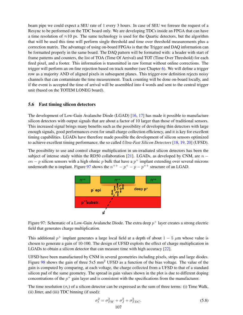
beam pipe we could expect a SEU rate of 1 every 3 hours. In case of SEU we foresee the request of aResync to be performed on the TDC board only. We are developing TDCs inside an FPGA that can havea time resolution of ≈10 ps. The same technology is used for the Quartic detectors, but the algorithmthat will be used this time will perform single threshold and time over threshold measurements plus acorrection matrix. The advantage of using on-board FPGAs is that the Trigger and DAQ information canbe formatted properly in the same board. The DAQ pattern will be formatted with: a header with start offrame patterns and counters, the list of TOA (Time Of Arrival) and TOT (Time Over Threshold) for eachfired pixel, and a footer. This information is transmitted in raw format without online corrections. Thetrigger will perform an on-line rejection based on track number (see Chapter 6). We will define a triggerrow as a majority AND of aligned pixels in subsequent planes. This trigger-row definition rejects noisychannels that can contaminate the time measurement. Track counting will be done on-board locally, andif the event is accepted the time of arrival will be assembled into 4 words and sent to the central triggerunit (based on the TOTEM LONEG board).

5.6 Fast timing silicon detectors

The development of Low-Gain Avalanche Diode (LGAD) [16, 17] has made it possible to manufacturesilicon detectors with output signals that are about a factor of 10 larger than those of traditional sensors.This increased signal brings many benefits such as the possibility of developing thin detectors with largeenough signals, good performances even for small charge collection efficiency, and it is key for excellenttiming capabilities. LGADs have therefore made possible the development of silicon sensors optimizedto achieve excellent timing performance, the so called Ultra-Fast Silicon Detectors [18, 19, 20] (UFSD).

The possibility to use and control charge multiplication in un-irradiated silicon detectors has been thesubject of intense study within the RD50 collaboration [21]. LGADs, as developed by CNM, are n −on − p silicon sensors with a high ohmic p bulk that have a p+ implant extending over several micronsunderneath the n-implant. Figure 97 shows the n++ − p+ − p− p++ structure of an LGAD.

Figure 97: Schematic of a Low-Gain Avalanche Diode. The extra deep p+ layer creates a strong electricfield that generates charge multiplication.

This additional p+ implant generates a large local field at a depth of about 1 − 5 µm whose value ischosen to generate a gain of 10-100. The design of UFSD exploits the effect of charge multiplication inLGADs to obtain a silicon detector that can measure time with high accuracy [22].

UFSD have been manufactured by CNM in several geometries including pixels, strips and large diodes.Figure 98 shows the gain of three 5x5 mm2 UFSD as a function of the bias voltage. The value of thegain is computed by comparing, at each voltage, the charge collected from a UFSD to that of a standardsilicon pad of the same geometry. The spread in gain values shown in the plot is due to different dopingconcentrations of the p+ gain layer and is consistent with the specifications from the manufacturer.

The time resolution (σt) of a silicon detector can be expressed as the sum of three terms: (i) Time Walk,(ii) Jitter, and (iii) TDC binning (if used):

σ2t = σ2

TW + σ2J + σ2

TDC . (5.8)

107

Figure 98: Value of the gain for three 5x5 mm2 UFSD as a function of the bias voltage. The value of thegain is computed by comparing, at each voltage, the charge collected from a UFSD to that of a standardsilicon pad of the same geometry.

The TDC binning introduces a fixed uncertainty equal to σTDC = TDCbin/√

12. As TDCs becomefaster and faster [23], we assume TDCbin = 20 ps and therefore this effect will not be important.

Using the explicit expressions of σTW , σJ and σTDC , Eq. ( 5.8) can be rewritten as:

σ2t = ([

Vth

S/tr]RMS)2 + (

N

S/tr)2 + (

TDCbin√12

)2, (5.9)

where

N: Noise: N ∝ CDet√tr. We assume it to be dominated by the voltage term.

S: Signal amplitude.

tr: Preamplifier rise time.

Vth: Comparator threshold.

TDCbin: TDC bin width. We assume a value of 20 ps.

To evaluate the performance of UFSD we have developed a simulation program called Weightfield2 [24].With the parametrization described in Eq.( 5.9), which is able to correctly reproduce the timing capa-bilities of state of the art silicon detectors, and the simulation program Weightfield2, which has beenvalidated using laboratory data, the timing capabilities of UFSD can be simulated.

As Eq.( 5.9) shows, time resolution is controlled, for constant noise N , by the ratio S/tr, which is therate dV/dt of the output signal of the detector: large dV/dt values are key to obtain excellent timeresolutions. Figure 99 shows, as a function of the internal gain, the simulated values of dV/dt for UFSDnormalized to that of a standard silicon sensor. The values of biasing voltage V shown in the legend aresuch that the sensors have the same electric fields. The figure shows that gain allows obtaining values ofdV/dt that are a factor of 5-10 higher than those of standard sensors.

108

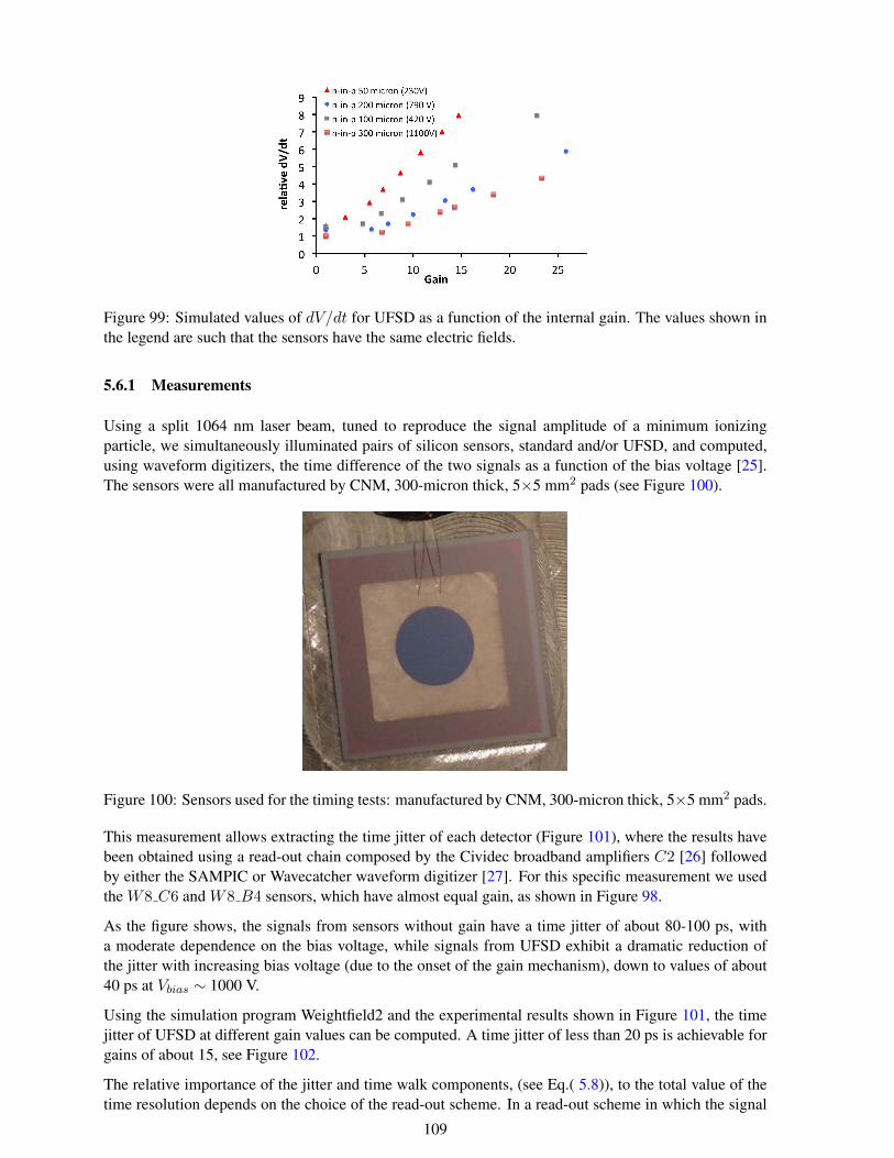
Figure 99: Simulated values of dV/dt for UFSD as a function of the internal gain. The values shown inthe legend are such that the sensors have the same electric fields.

5.6.1 Measurements

Using a split 1064 nm laser beam, tuned to reproduce the signal amplitude of a minimum ionizingparticle, we simultaneously illuminated pairs of silicon sensors, standard and/or UFSD, and computed,using waveform digitizers, the time difference of the two signals as a function of the bias voltage [25].The sensors were all manufactured by CNM, 300-micron thick, 5×5 mm2 pads (see Figure 100).

Figure 100: Sensors used for the timing tests: manufactured by CNM, 300-micron thick, 5×5 mm2 pads.

This measurement allows extracting the time jitter of each detector (Figure 101), where the results havebeen obtained using a read-out chain composed by the Cividec broadband amplifiers C2 [26] followedby either the SAMPIC or Wavecatcher waveform digitizer [27]. For this specific measurement we usedthe W8 C6 and W8 B4 sensors, which have almost equal gain, as shown in Figure 98.

As the figure shows, the signals from sensors without gain have a time jitter of about 80-100 ps, witha moderate dependence on the bias voltage, while signals from UFSD exhibit a dramatic reduction ofthe jitter with increasing bias voltage (due to the onset of the gain mechanism), down to values of about40 ps at Vbias ∼ 1000 V.

Using the simulation program Weightfield2 and the experimental results shown in Figure 101, the timejitter of UFSD at different gain values can be computed. A time jitter of less than 20 ps is achievable forgains of about 15, see Figure 102.

The relative importance of the jitter and time walk components, (see Eq.( 5.8)), to the total value of thetime resolution depends on the choice of the read-out scheme. In a read-out scheme in which the signal

109

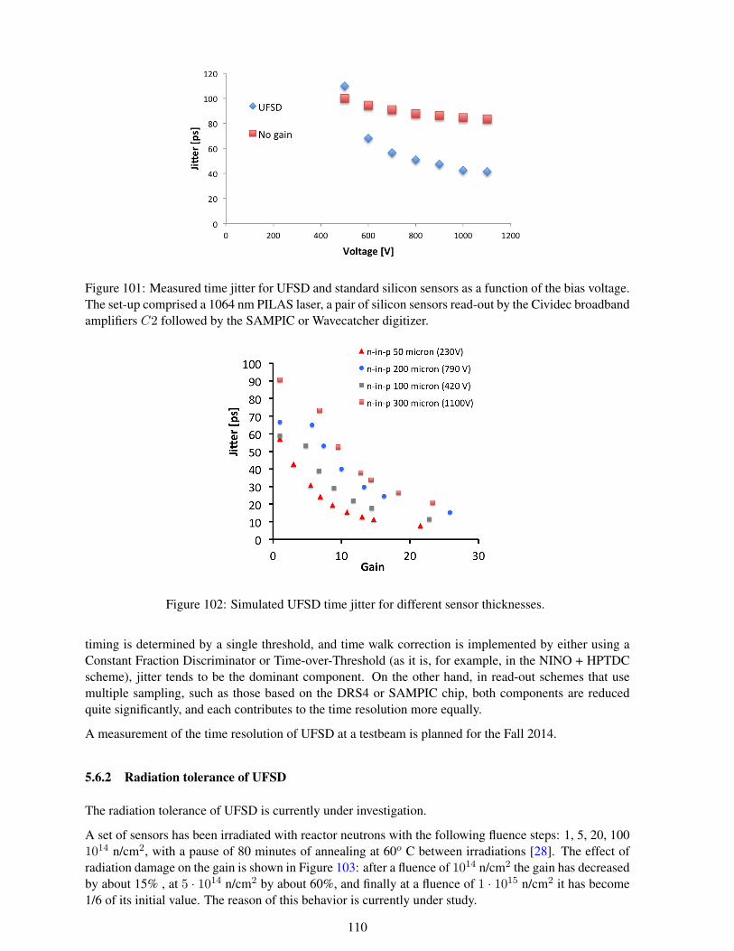
Figure 101: Measured time jitter for UFSD and standard silicon sensors as a function of the bias voltage.The set-up comprised a 1064 nm PILAS laser, a pair of silicon sensors read-out by the Cividec broadbandamplifiers C2 followed by the SAMPIC or Wavecatcher digitizer.

Figure 102: Simulated UFSD time jitter for different sensor thicknesses.

timing is determined by a single threshold, and time walk correction is implemented by either using aConstant Fraction Discriminator or Time-over-Threshold (as it is, for example, in the NINO + HPTDCscheme), jitter tends to be the dominant component. On the other hand, in read-out schemes that usemultiple sampling, such as those based on the DRS4 or SAMPIC chip, both components are reducedquite significantly, and each contributes to the time resolution more equally.

A measurement of the time resolution of UFSD at a testbeam is planned for the Fall 2014.

5.6.2 Radiation tolerance of UFSD

The radiation tolerance of UFSD is currently under investigation.

A set of sensors has been irradiated with reactor neutrons with the following fluence steps: 1, 5, 20, 1001014 n/cm2, with a pause of 80 minutes of annealing at 60o C between irradiations [28]. The effect ofradiation damage on the gain is shown in Figure 103: after a fluence of 1014 n/cm2 the gain has decreasedby about 15% , at 5 · 1014 n/cm2 by about 60%, and finally at a fluence of 1 · 1015 n/cm2 it has become1/6 of its initial value. The reason of this behavior is currently under study.

110

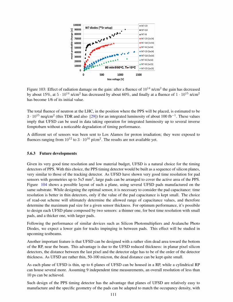
Figure 103: Effect of radiation damage on the gain: after a fluence of 1014 n/cm2 the gain has decreasedby about 15%, at 5 · 1014 n/cm2 has decreased by about 60%, and finally at a fluence of 1 · 1015 n/cm2

has become 1/6 of its initial value.

The total fluence of neutron at the LHC, in the position where the PPS will be placed, is estimated to be3 · 1015 neq/cm2 (this TDR and also [29]) for an integrated luminosity of about 100 fb−1. These valuesimply that UFSD can be used in data taking operation for integrated luminosity up to several inversefemptobarn without a noticeable degradation of timing performance.

A different set of sensors was been sent to Los Alamos for proton irradiation; they were exposed tofluences ranging from 1012 to 3 · 1016 p/cm2. The results are not available yet.

5.6.3 Future developments

Given its very good time resolution and low material budget, UFSD is a natural choice for the timingdetectors of PPS. With this choice, the PPS timing detector would be built as a sequence of silicon planes,very similar to those of the tracking detector. As UFSD have shown very good time resolution for padsensors with geometries up to 5x5 mm2, large pads can be arranged to cover the active area of the PPS.Figure 104 shows a possible layout of such a plane, using several UFSD pads manufactured on thesame substrate. While designing the optimal sensor, it is necessary to consider the pad capacitance: timeresolution is better in thin detectors, only if the value of the pad capacitance is kept small. The choiceof read-out scheme will ultimately determine the allowed range of capacitance values, and thereforedetermine the maximum pad size for a given sensor thickness. For optimum performance, it’s possibileto design each UFSD plane composed by two sensors: a thinner one, for best time resolution with smallpads, and a thicker one, with larger pads.

Following the performance of similar devices such as Silicon Photomultipliers and Avalanche PhotoDiodes, we expect a lower gain for tracks impinging in between pads. This effect will be studied inupcoming testbeams.

Another important feature is that UFSD can be designed with a rather slim dead area toward the bottomof the RP, near the beam. This advantage is due to the UFSD reduced thickness: in planar pixel silicondetectors, the distance between the last pixel and the detector edge has to be of the order of the detectorthickness. As UFSD are rather thin, 50-100 micron, the dead distance can be kept quite small.

As each plane of UFSD is thin, up to 6 planes of UFSD can be housed in a RP, while a cylindrical RPcan house several more. Assuming 9 independent time measurements, an overall resolution of less than10 ps can be achieved.

Such design of the PPS timing detector has the advantage that planes of UFSD are relatively easy tomanufacture and the specific geometry of the pads can be adapted to match the occupancy density, with

111

Figure 104: Possible layout of a single plane for the timing detector of the PPS. Each plane is composedof several UFSD pads manufactured on the same substrate. The size of each pad reflects the varyingoccupancy of the detector.

smaller pads at the center of the detector plane, near the beampipe. They have a very low material budget,and the cost for full set of planes plus spares (24 + 24) is around 40k Euros.

We are currently in the process of manufacture two additional sets of sensors: the first one will be ona 200-micron thick FZ substrate, and will use either boron and indium as dopant for the gain layer.This production, expected in the Fall of 2014, will help us consolidate the design process, compare theperformance of 300- and 200-micron thick sensors, and measure the radiation hardness of indium-dopedsensors. The second production, aimed for the Spring 2015, will use 50- and 100-micron SOI sensors,and it will have full PPS sensor geometry. As time resolution improves for reduced sensor thickness,we expect the 50- and 100-micron thick detector to achieve a significant break-through in performance,allowing us to manufacture the final UFSD sensor geometry for the PPS for the Fall 2015.

The read-out electronics for such a detector can either be derived from the configuration that was usedin the tests presented above (a broadband amplifier followed by a waveform digitizer), or can be adaptedfrom the electronics developed for diamond and silicon multi-layers detectors [30].

The aim of the group developing SAMPIC is to obtain a system able to achieve sub-10 ps timing resolu-tion, 1GHz input bandwidth, no dead time at the LHC, and data taking at 2 Gigasamples per second. Thepresent version does not match these requirements and does not have trigger capability at the cell level.An upgrade of SAMPIC with several of these features will be available by the end of 2014. The cost perchannel is estimated to be of the order of 10$.

5.6.4 3D silicon sensors

3D sensors, already considered as baseline for the PPS tracking system, can be considered promisingcandidates also for timing measurements. Thanks to their unique structure, very short drift times canbe achieved by choosing small inter-electrode spacing without reducing the substrate thickness, thuspreserving the signal amplitude. TCAD simulations show that a rise time and a collection time of 10 psand 500 ps respectively can be achieved for inter-electrode distance of 50 micron. First measurementsperformed with a non optimized readout electronics have shown that resolutions between 30 and 180 ps,

112

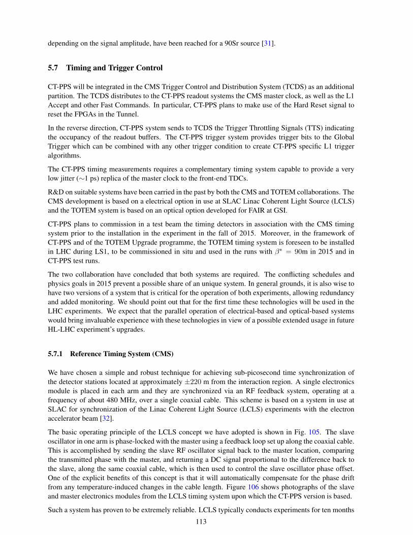
depending on the signal amplitude, have been reached for a 90Sr source [31].

5.7 Timing and Trigger Control

CT-PPS will be integrated in the CMS Trigger Control and Distribution System (TCDS) as an additionalpartition. The TCDS distributes to the CT-PPS readout systems the CMS master clock, as well as the L1Accept and other Fast Commands. In particular, CT-PPS plans to make use of the Hard Reset signal toreset the FPGAs in the Tunnel.

In the reverse direction, CT-PPS system sends to TCDS the Trigger Throttling Signals (TTS) indicatingthe occupancy of the readout buffers. The CT-PPS trigger system provides trigger bits to the GlobalTrigger which can be combined with any other trigger condition to create CT-PPS specific L1 triggeralgorithms.

The CT-PPS timing measurements requires a complementary timing system capable to provide a verylow jitter (∼1 ps) replica of the master clock to the front-end TDCs.

R&D on suitable systems have been carried in the past by both the CMS and TOTEM collaborations. TheCMS development is based on a electrical option in use at SLAC Linac Coherent Light Source (LCLS)and the TOTEM system is based on an optical option developed for FAIR at GSI.

CT-PPS plans to commission in a test beam the timing detectors in association with the CMS timingsystem prior to the installation in the experiment in the fall of 2015. Moreover, in the framework ofCT-PPS and of the TOTEM Upgrade programme, the TOTEM timing system is foreseen to be installedin LHC during LS1, to be commissioned in situ and used in the runs with β∗ = 90m in 2015 and inCT-PPS test runs.

The two collaboration have concluded that both systems are required. The conflicting schedules andphysics goals in 2015 prevent a possible share of an unique system. In general grounds, it is also wise tohave two versions of a system that is critical for the operation of both experiments, allowing redundancyand added monitoring. We should point out that for the first time these technologies will be used in theLHC experiments. We expect that the parallel operation of electrical-based and optical-based systemswould bring invaluable experience with these technologies in view of a possible extended usage in futureHL-LHC experiment’s upgrades.

5.7.1 Reference Timing System (CMS)

We have chosen a simple and robust technique for achieving sub-picosecond time synchronization ofthe detector stations located at approximately ±220 m from the interaction region. A single electronicsmodule is placed in each arm and they are synchronized via an RF feedback system, operating at afrequency of about 480 MHz, over a single coaxial cable. This scheme is based on a system in use atSLAC for synchronization of the Linac Coherent Light Source (LCLS) experiments with the electronaccelerator beam [32].

The basic operating principle of the LCLS concept we have adopted is shown in Fig. 105. The slaveoscillator in one arm is phase-locked with the master using a feedback loop set up along the coaxial cable.This is accomplished by sending the slave RF oscillator signal back to the master location, comparingthe transmitted phase with the master, and returning a DC signal proportional to the difference back tothe slave, along the same coaxial cable, which is then used to control the slave oscillator phase offset.One of the explicit benefits of this concept is that it will automatically compensate for the phase driftfrom any temperature-induced changes in the cable length. Figure 106 shows photographs of the slaveand master electronics modules from the LCLS timing system upon which the CT-PPS version is based.

Such a system has proven to be extremely reliable. LCLS typically conducts experiments for ten months

113

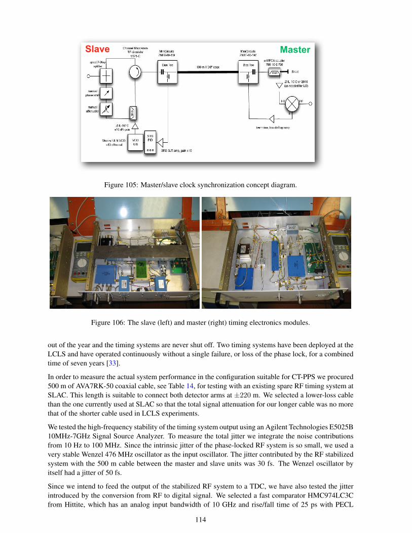
Slave Master

Figure 105: Master/slave clock synchronization concept diagram.

Figure 106: The slave (left) and master (right) timing electronics modules.

out of the year and the timing systems are never shut off. Two timing systems have been deployed at theLCLS and have operated continuously without a single failure, or loss of the phase lock, for a combinedtime of seven years [33].

In order to measure the actual system performance in the configuration suitable for CT-PPS we procured500 m of AVA7RK-50 coaxial cable, see Table 14, for testing with an existing spare RF timing system atSLAC. This length is suitable to connect both detector arms at ±220 m. We selected a lower-loss cablethan the one currently used at SLAC so that the total signal attenuation for our longer cable was no morethat of the shorter cable used in LCLS experiments.

We tested the high-frequency stability of the timing system output using an Agilent Technologies E5025B10MHz-7GHz Signal Source Analyzer. To measure the total jitter we integrate the noise contributionsfrom 10 Hz to 100 MHz. Since the intrinsic jitter of the phase-locked RF system is so small, we used avery stable Wenzel 476 MHz oscillator as the input oscillator. The jitter contributed by the RF stabilizedsystem with the 500 m cable between the master and slave units was 30 fs. The Wenzel oscillator byitself had a jitter of 50 fs.

Since we intend to feed the output of the stabilized RF system to a TDC, we have also tested the jitterintroduced by the conversion from RF to digital signal. We selected a fast comparator HMC974LC3Cfrom Hittite, which has an analog input bandwidth of 10 GHz and rise/fall time of 25 ps with PECL

114

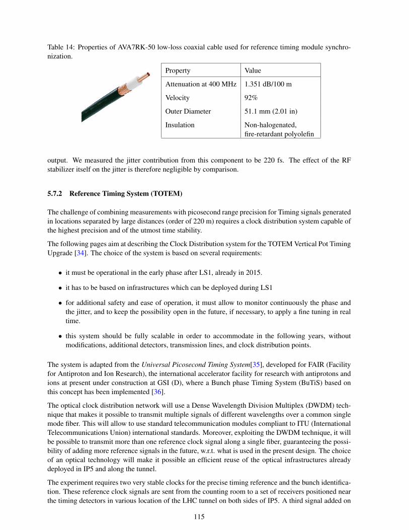
Table 14: Properties of AVA7RK-50 low-loss coaxial cable used for reference timing module synchro-nization.

Property Value

Attenuation at 400 MHz 1.351 dB/100 m

Velocity 92%

Outer Diameter 51.1 mm (2.01 in)

Insulation Non-halogenated,fire-retardant polyolefin

output. We measured the jitter contribution from this component to be 220 fs. The effect of the RFstabilizer itself on the jitter is therefore negligible by comparison.

5.7.2 Reference Timing System (TOTEM)

The challenge of combining measurements with picosecond range precision for Timing signals generatedin locations separated by large distances (order of 220 m) requires a clock distribution system capable ofthe highest precision and of the utmost time stability.

The following pages aim at describing the Clock Distribution system for the TOTEM Vertical Pot TimingUpgrade [34]. The choice of the system is based on several requirements:

• it must be operational in the early phase after LS1, already in 2015.

• it has to be based on infrastructures which can be deployed during LS1

• for additional safety and ease of operation, it must allow to monitor continuously the phase andthe jitter, and to keep the possibility open in the future, if necessary, to apply a fine tuning in realtime.

• this system should be fully scalable in order to accommodate in the following years, withoutmodifications, additional detectors, transmission lines, and clock distribution points.

The system is adapted from the Universal Picosecond Timing System[35], developed for FAIR (Facilityfor Antiproton and Ion Research), the international accelerator facility for research with antiprotons andions at present under construction at GSI (D), where a Bunch phase Timing System (BuTiS) based onthis concept has been implemented [36].

The optical clock distribution network will use a Dense Wavelength Division Multiplex (DWDM) tech-nique that makes it possible to transmit multiple signals of different wavelengths over a common singlemode fiber. This will allow to use standard telecommunication modules compliant to ITU (InternationalTelecommunications Union) international standards. Moreover, exploiting the DWDM technique, it willbe possible to transmit more than one reference clock signal along a single fiber, guaranteeing the possi-bility of adding more reference signals in the future, w.r.t. what is used in the present design. The choiceof an optical technology will make it possible an efficient reuse of the optical infrastructures alreadydeployed in IP5 and along the tunnel.

The experiment requires two very stable clocks for the precise timing reference and the bunch identifica-tion. These reference clock signals are sent from the counting room to a set of receivers positioned nearthe timing detectors in various location of the LHC tunnel on both sides of IP5. A third signal added on

115

the same optical fiber will be simply reflected back to be used to continuously measure the time delay ofeach optical transmission line: these delay measurements are necessary to correct the time informationgenerated at the detector location for fiber delay variations (thermal and mechanical instabilities). In ad-dition, this will allow an event by event monitor of the status of the clock signals, opening the possibilityof adding these informations to the data stream as well.

The system can be logically subdivided in four major blocks: the Transmission Unit, the DistributionUnit, the Measurement Unit and the Receiving Unit. One Receiving Unit must be installed very neareach RP location, the Transmission, Distribution and Measurement Units will be located in the TOTEMracks in the IP5 counting room. A block diagram of the entire system is reproduced in Figure 107.

Measurements performed with the prototype of the “BuTiS” system show that the influence of the trans-mission system on the signal jitter, is of the order of 0.4 ps [36], mainly dependent on the quality ofthe clock source signal, the noise added by the optical components and the bandwidth of the transmis-sion system itself. Using a transmission system based on this concept, the total jitter of the TOTEMclock transmission system will also be due mainly to the inherent jitter of clock sources and the end userelectronics.

Transmission Unit

The Transmission Unit optically modulates the two reference clocks in signals with different wavelengthλ1 and λ2. Via DWDM these optical signal are multiplexed into a single fiber and re-transmitted at aspecific wavelength using a 1,550 nm band laser to the Distribution Unit. The signal is amplified withan erbium-doped fiber amplifier (EDFA) to compensate the attenuation due to further splitting and themultiplexers.

A Thorlabs PRO8000‡ platform has been chosen to generate the two DWDM wavelengths on chan-nels ITU 32 and ITU 34 . This complete platform is designed to operate and control electrical andoptical modules for telecommunication testing and application developments from a broad family of in-terchangeable modular devices and can be controlled by an external computer using industrial controlprotocols. The modulation of the optical signals is performed by two military grade Mach-Zehnder mod-ulators of 20GHz bandwidth. The EDFA amplifier developed for this platform will be used. This unitcan be rack mounted and is suitable for use in the experiment control room harsh environment.

Distribution Unit

The DWDM optical signal, as generated by the Transmission Unit, needs to be split in order to be trans-mitted to the four Receiving Units. Moreover a third DWDM modulated optical signal of wavelengthλM is needed to measure the transmission delays over each fiber and is added to the other two clocksignals.

The JDSU§ Multiple Application Platform (MAP-200) has been chosen for the Distribution Unit opticalamplification. This platform is a highly configurable, scalable and industrially controlled system that canhost several optical modules with a wide range of functions.

‡Thorlabs, Inc. : www.thorlabs.com. PRO8000 platform: http://www.thorlabs.com/newgrouppage9.cfm?objectgroup id=895.

§JDS Uniphase Corporation: www.jdsu.com. Multiple Application Platform (MAP-200): http://www.jdsu.com/en-us/test-and-measurement/products/a-z-product-list/Pages/map.aspx .

116

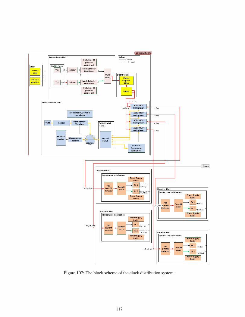
Figure 107: The block scheme of the clock distribution system.

117

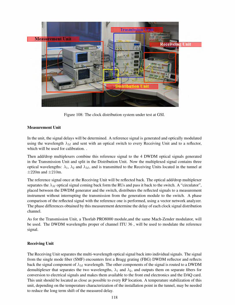
Figure 108: The clock distribution system under test at GSI.

Measurement Unit

In the unit, the signal delays will be determined. A reference signal is generated and optically modulatedusing the wavelength λM and sent with an optical switch to every Receiving Unit and to a reflector,which will be used for calibration. .

Then add/drop multiplexers combine this reference signal to the 4 DWDM optical signals generatedin the Transmission Unit and split in the Distribution Unit. Now the multiplexed signal contains threeoptical wavelengths: λ1, λ2 and λM , and is transmitted to the Receiving Units located in the tunnel at±220m and ±210m.

The reference signal once at the Receiving Unit will be reflected back. The optical add/drop multiplexerseparates the λM optical signal coming back form the RUs and pass it back to the switch. A “circulator”,placed between the DWDM generator and the switch, distributes the reflected signals to a measurementinstrument without interrupting the transmission from the generation module to the switch. A phasecomparison of the reflected signal with the reference one is performed, using a vector network analyzer.The phase differences obtained by this measurement determine the delay of each clock signal distributionchannel.

As for the Transmission Unit, a Thorlab PRO8000 module,and the same Mach-Zender modulator, willbe used. The DWDM wavelengths proper of channel ITU 36 , will be used to modulate the referencesignal.

Receiving Unit

The Receiving Unit separates the multi-wavelength optical signal back into individual signals. The signalfrom the single mode fiber (SMF) encounters first a Bragg grating (FBG) DWDM reflector and reflectsback the signal component of λM wavelength. The other components of the signal is routed to a DWDMdemultiplexer that separates the two wavelengths, λ1 and λ2, and outputs them on separate fibers forconversion to electrical signals and makes them available to the front end electronics and the DAQ card.This unit should be located as close as possible to every RP location. A temperature stabilization of thisunit, depending on the temperature characterization of the installation point in the tunnel, may be neededto reduce the long term shift of the measured delay.

118

5.8 Plans and Schedule

An important objective of the CT-PPS exploratory phase (2015-16) is to demonstrate the timing perfor-mance and the pile-up rejection capabilities of the baseline detector. We plan to carry out this activityin the fall of 2015 and beginning of 2016, after the programme of validation of RP operation at highluminosity described in 1.3.

The baseline Quartic detector modules will be evaluated in test beams in the Spring-Summer 2015, whenthe readout system will become available. GasToF prototype modules will be built and will also beevaluated in the same test beam. In parallel an extensive R&D programme on the timing solid statetechnologies will be carried including test beam activities.

The integration of the local DAQ hardware and online software in the central CMS Trigger/DAQ systemand clock distribution system (TCDS) will be tested in the CMS Electronics Integration Center in theSpring-Summer 2015.

The Quartic detector and the front-end readout system is expected to be ready for installation in thecylindrical RPs in the fall of 2015. One cylindrical RP per arm has already been installed in LS1, allowingthe installation Quartic timing detectors during a short technical stop. The installation procedure will betested beforehand in the lab using a spare cylindrical pot.

References

[1] M.G. Albrow et al., “The FP420 R&D Project: Higgs and New Physics with forward protons atLHC”, JINST 4 (2009) T10001.

[2] L. Bonnet, J. Liao and K. Piotrzkowski, “Study on GasToF: A 10 ps resolution timing detector”,NIM A762 (2014) 77.

[3] M.G.Albrow, “Fast timing detectors for leading protons at LHC: QUARTIC”, Proc. Workshop onPicosecond Photon Sensors for Physics and Medical Applications, Clermont-Ferrand, March 2014(to be published in Acta Physica Polonica).

[4] G. Chiodini, “Timing Diamond Detector for MIP”, Workshop on Picosecond Photon Sensors forPhysics and Medical Applications, Clermont-Ferrand, March 2014.

[5] M. Ciobanu et al., “In-beam diamond start detectors”, IEEE Trans. Nucl. Sci. 58 (2011) 2073.

[6] N. Cartiglia et al., “Timing capabilities of Ultra-Fast Silicon Detector”, Workshop on PicosecondPhoton Sensors for Physics and Medical Applications, Clermont-Ferrand, March 2014

[7] CMS Technical Design Report for the Phase 1 Upgrade of the Hadron Calorimeter, Technical Re-port CERN-LHCC-2012-015. CMS-TDR-010, CERN, Geneva, (Sep, 2012).

[8] M.G. Albrow et al., “Quartz Cherenkov counters for fast timing: QUARTIC”, JInst 7 P10027(2012).

[9] M. Mazzillo et al., IEEE Nucl. Sci. Symposium NI-187 p.391.

[10] A. Ronzhin et al., “Tests of timing properties of silicon photomultipliers”, NIM A616 (2010) 38.

[11] J. Va’vra et al., “Beam Test of a Time-of-Flight Detector Prototype”, NIM A606 (2009) 404.

[12] Specialty Glass Products, 2885 Terwood Rd., Willow Grove, PA 19090, USA.

[13] http://www.photonis.com/en/ism/63-planacon.html

119

http://www.photonis.com/en/ism/63-planacon.html

[14] S. Gundacker et al., “Time of flight positron emission tomography towards 100 ps resolution withL(Y)SO: an experimental and theoretical analysis”, JINST 8 (2013) P07014.

[15] F. Anghinolfi et al. “NINO: an ultra-fast and low-power front-end amplifier/discriminator ASICdesigned for the multigap resistive plate chamber”. NIM A 533 (2004) 183.

[16] P. Fernandez et al, “ Simulation of new p-type strip detectors with trench to enhance the chargemultiplication effect in the n-type electrodes”, NIM A 658 (2011) 98.

[17] G. Pellegrini et al., “Technology developments and first measurements of Low Gain AvalancheDetectors (LGAD) for High Energy Physics applications”, Hiroshima Conference, HSTD9, Hi-roshima, Japan, NIM A, in print (2014).

[18] H. F. W. Sadrozinski, “Exploring charge multiplication for fast timing with silicon sen-sors”, 20th RD50 Workshop, Bari, Italy, May 30-June 1, 2012, and references thereinhttps://indico.cern.ch/conferenceOtherViews.py?view=standard&confId=175330.

[19] H. F. W. Sadrozinski, S. Ely, V. Fadeyev, Z. Galloway, J. Ngo, C. Parker, B. Petersen and A. Seidenet al., “Ultra-fast silicon detectors,” Nucl. Instrum. Meth. A 730 (2013) 226.

[20] H. F. W. Sadrozinski et al., “Sensors for Ultra-Fast Silicon Detectors”, HSTD9, Hiroshima, Japan.NIM A, in print.

[21] RD50 collaboration,http://rd50.web.cern.ch/rd50/.

[22] N Cartiglia et al., “Performance of ultra-fast silicon detectors”, JINST 9 (2014) C02001.

[23] A. Rivetti, et al.,“Electronics for Fast Tracking Detector”, HSTD9, Hiroshima, Japan. NIM A, inprint.

[24] F. Cenna et al, “Weightfield2”, 9th Trento Workshop on Innovative Silicon Detector, Genova, 2014.available at http://personalpages.to.infn.it/∼cartigli/weightfield2

[25] R. Arcidiacono et al, “Timing properties of Ultra-Fast Silicon Detectors”, 2nd Workshopon Detectors for Forward Physics at LHC, http://indico.cern.ch/event/295567/other-view?view=standard

[26] http://www.cividec.at/.

[27] E. Delagnes, D. Breton, F. Lugiez, R. Rahmanifard, “A low power multi-channel single ramp ADCwith up to 3.2 GHz virtual clock”, IEEE Trans. Nucl. Science 54 (2007) 1735.

[28] G. Kramberger et al, “ Radiation hardness of Low Gain Amplification Diodes (LGAD)”, 9th TrentoWorkshop on Innovative Silicon Detector, Genova, 2014.

[29] M. Dyndal et al, “The tracking System of APF”, 2nd Workshop on Detectors for Forward Physicsat LHC, http://indico.cern.ch/event/295567/session/2/contribution/9/material/slides/0.pdf

[30] R. Cardarelli, “Development of Diamond and Silicon Multi-Layer Detector and related front-endelectronics, 2nd Workshop on Detectors for Forward Physics at LHC”, http://indico.cern.ch/event/295567/other-view?view=standard

[31] S. Parker et al, “Increased speed: 3D silicon sensors; fast current amplifiers”, Nucl. Science IEEETransactions, Volumes 58, Issue 2, April 2011.

[32] J. Frisch et al., “Status of the LCLS Experiment Timing System”, Proceedings of IBIC2012,Tsukuba, Japan (2012), SLAC-PUB-15254.

120

http://rd50.web.cern.ch/rd50/

http://personalpages.to.infn.it/~cartigli/weightfield2

http://indico.cern.ch/event/295567/other-view?view=standard


http://www.cividec.at/

http://indico.cern.ch/event/295567/session/2/contribution/9/material/slides/0.pdf

http://indico.cern.ch/event/295567/session/2/contribution/9/material/slides/0.pdf



[33] S. Smith SLAC, private communication, July 31, 2014.

[34] TOTEM Collaboration, “TOTEM Upgrade Proposal”, CERN-LHCC-2013-009; LHCC-P-007 and“Timing Measurements in the Vertical Roman Pots of the TOTEM Experiment”, CERN-LHCC-2014-020 (TOTEM-TDR-002).

[35] Bousonville, M. and Rausch, J., “Universal picosecond timing system for the Facility for Antiprotonand Ion Research”, Phys. Rev. ST Accel. Beams 12 (2009) 042801.http://link.aps.org/doi/10.1103/PhysRevSTAB.12.042801

[36] P. Moritz and B. Zipfel. “Recent Progress on the Technical Realization of the Bunch Phase 701Timing System BuTiS”, Conf.Proc., C110904 (2011) 418.

121

http://link.aps.org/doi/10.1103/PhysRevSTAB.12.042801

6 Trigger Strategy

The triggers used for CT-PPS physics are expected to capture the interesting final states in the kinematicalrange covered by the PPS acceptance with large efficiency (see Chapters 1 and 2). In the followingdiscussion we distinguish leptonic and hadronic final states, and we consider separately physics processeswith small and large cross-section, as the trigger strategy depends strongly on these cases.

In two-photon physics the main exclusive states are X = e+e−, µ+µ−, τ+τ− and W+W− in the highmass region (≥ 300 GeV), which is accessible to CT-PPS with both protons detected. The leptonic finalstates are captured by the full suite of CMS lepton triggers (single and double). The trigger efficiencyin these cases is expected to be very high given that the lepton thresholds are at the level of 30 GeVor below. Final states with hadronic decays of one W or one tau will be accessible using the suite oflepton+jet triggers. Again, the foreseen CMS thresholds are sufficiently low to guarantee high efficiencyin the kinematical region covered by PPS. Table 15, taken from the CMS L1 Trigger Upgrade TDR ([1]),shows the menu of main L1 Triggers at the instantaneous luminosity of 2× 1034 cm−2 s−1. In the HighLevel Trigger (HLT) the thresholds are 20-30% higher.

Trigger Rate 95% Threshold PlateauAlgorithm [kHz] [GeV] EfficiencySingle e/γ 11 57 1.0Single iso e/γ 15 31 0.9Single Mu 14 22 0.9Single iso Mu 15 19 0.82Single Tau 12 100 0.95Single iso Tau 13 83 0.7iso e/γ + e/γ 12 23 16 0.9(iso)Mu+Mu 9.4 15 10 0.8(iso)Tau+Tau 7.2 64 62 0.67iso e/γ + Mu 11 21 10 0.85(iso)Mu + e/γ 8.3 18 15 0.83iso e/γ + Tau 8.3 21 57 0.86isoMu + Tau 5.8 14 47 0.8Single Jet 5.9 205 1.0Double Jet 4.2 130 130 1.0Quad Jet 5.0 4@55 1.0Single iso e/γ + Jet 11 27 78 0.9Single Mu + Jet 9.7 18 52 0.93Single iso e/γ + Hmiss

T 12 27 110 0.9Single Mu + Hmiss

T 11 18 86 0.93HT 3.0 380 1.0Total Rate 95

Table 15: L1 trigger menu and estimated rates in Run2 (energy 14 TeV, L = 2.2×1034 cm−2 s−1, bunchspacing of 25 ns, pile-up of 50).

In case the CT-PPS detectors could be operated at a distance from the beam smaller than the baseline of15 sigma, increasing the acceptance at low masses (≥ 100-200 GeV), the lepton and lepton+jets centraltriggers would need to be combined with trigger information provided by the CT-PPS detectors. Belowwe discuss possible strategies.

The trigger requirements for the CT-PPS jet physics are more complicated because the inclusive QCDjet background is very large, even for the relatively large jet thresholds that match to the CT-PPS massacceptance. Jet rates above the allowed L1 or HLT bandwidth will require the addition of cuts on theprotons kinematics.

At HLT, we may require events with protons detected in both CT-PPS arms. While under large pileup

122

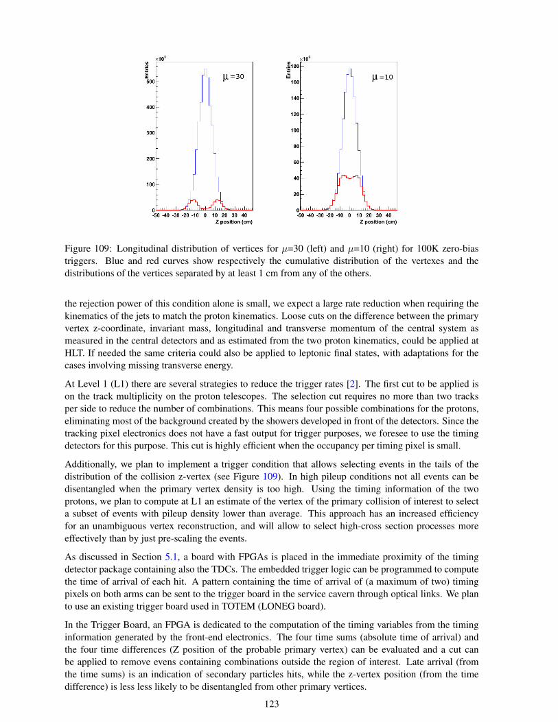
Figure 109: Longitudinal distribution of vertices for µ=30 (left) and µ=10 (right) for 100K zero-biastriggers. Blue and red curves show respectively the cumulative distribution of the vertexes and thedistributions of the vertices separated by at least 1 cm from any of the others.

the rejection power of this condition alone is small, we expect a large rate reduction when requiring thekinematics of the jets to match the proton kinematics. Loose cuts on the difference between the primaryvertex z-coordinate, invariant mass, longitudinal and transverse momentum of the central system asmeasured in the central detectors and as estimated from the two proton kinematics, could be applied atHLT. If needed the same criteria could also be applied to leptonic final states, with adaptations for thecases involving missing transverse energy.

At Level 1 (L1) there are several strategies to reduce the trigger rates [2]. The first cut to be applied ison the track multiplicity on the proton telescopes. The selection cut requires no more than two tracksper side to reduce the number of combinations. This means four possible combinations for the protons,eliminating most of the background created by the showers developed in front of the detectors. Since thetracking pixel electronics does not have a fast output for trigger purposes, we foresee to use the timingdetectors for this purpose. This cut is highly efficient when the occupancy per timing pixel is small.

Additionally, we plan to implement a trigger condition that allows selecting events in the tails of thedistribution of the collision z-vertex (see Figure 109). In high pileup conditions not all events can bedisentangled when the primary vertex density is too high. Using the timing information of the twoprotons, we plan to compute at L1 an estimate of the vertex of the primary collision of interest to selecta subset of events with pileup density lower than average. This approach has an increased efficiencyfor an unambiguous vertex reconstruction, and will allow to select high-cross section processes moreeffectively than by just pre-scaling the events.

As discussed in Section 5.1, a board with FPGAs is placed in the immediate proximity of the timingdetector package containing also the TDCs. The embedded trigger logic can be programmed to computethe time of arrival of each hit. A pattern containing the time of arrival of (a maximum of two) timingpixels on both arms can be sent to the trigger board in the service cavern through optical links. We planto use an existing trigger board used in TOTEM (LONEG board).

In the Trigger Board, an FPGA is dedicated to the computation of the timing variables from the timinginformation generated by the front-end electronics. The four time sums (absolute time of arrival) andthe four time differences (Z position of the probable primary vertex) can be evaluated and a cut canbe applied to remove evens containing combinations outside the region of interest. Late arrival (fromthe time sums) is an indication of secondary particles hits, while the z-vertex position (from the timedifference) is less less likely to be disentangled from other primary vertices.

123

In a MC study [2], based on inclusive DPE events and with pileup µ = 50, cuts on the sums anddifferences of the four proton arrival time combinations are applied in order to optimize the isolationof the primary vertex for a given time detector resolution (a resolution of 25 ps was assumed). In thisconfiguration a rate of 47 kHz (RP double arm) is achieved, with a purity of the DPE sample of 0.12 anda trigger efficiency of 9%.

The LONEG board is connected with 8 bits to the L1 trigger. Originated at 210 m from the IP, a trig-ger signal can be included within the CMS L1 latency. The algorithms foreseen for the multi-jet finalstates are a combination with different di-jet trigger algorithms with the protons. An optimization of jetthresholds has to be made in function of the machine luminosity.

In a future upgrade of the timing detectors, a L1 CT-PPS trigger based on high granularity and multi-layer detectors capable to compute the two-proton kinematics and compare it with the kinematics of thecentrally produced system would be desirable. The proposed R&D program includes the developmentof suitable integrate circuits building upon the existing TOFPET chip developed by an institute of thecollaboration [3].

References

[1] CMS Technical Design Report for the Level-1 Trigger Upgrade, Technical Report CERN-LHCC-2013-011. CMS-TDR-012, CERN, Geneva, (Aug. 2013).

[2] M. Berretti, “Performance studies of the Roman Pot timing detectors in the forward region of theIP5 at LHC”, TOTEM-NOTE 2014-001.

[3] M. Rolo et al., “TOFPET ASIC for PET applications”, JINST 8, C02050, Feb 2013.

124

7 Organization, Responsibilities and Cost

7.1 Participating Institutes

The institutes of the CMS and TOTEM Collaborations presently involved in the CT-PPS project are listedbelow.

CMS Collaboration

1. Universite Catholique de Louvain, Louvain-la-Neuve, BELGIUM

2. Universidade do Estado do Rio de Janeiro, BRAZIL

3. Centro Brasileiro de Pesquisas Fisicas, Rio de Janeiro, BRAZIL

4. IPM, Institute for Research in Fundamental Sciences, Tehran, IRAN

5. Universita di Genova and INFN Sezione di Genova, ITALY

6. Universita di Torino, Universita del Piemonte Orientale, Novara, and INFN Sezione di Torino,ITALY

7. LIP, Laboratorio de Instrumentacao e Fısica Experimental de Partıculas, Lisboa, PORTUGAL

8. Institute for High Energy Physics, Protvino, RUSSIA

9. CERN, European Organization for Nuclear Research, Geneva, SWITZERLAND

10. Fermi National Accelerator Laboratory, Batavia, Illinois, USA

11. Lawrence Livermore National Laboratory, USA

12. The University of Kansas, Kansas Lawrence, USA

13. The University of Iowa, Iowa City, USA

14. The Rockefeller University, New York, USA

TOTEM Collaboration

1. Institute of Physics of the ASCR, Prague, CZECH REPUBLIC

2. University of West Bohemia, Pilsen, CZECH REPUBLIC

3. Helsinki Institute of Physics and Department of Physics, University of Helsinki, FINLAND

4. INFN Sezione di Bari, Universita di Bari and Politecnico di Bari, ITALY

5. Universita di Siena and INFN Sezione di Pisa, ITALY

6. CERN, European Organization for Nuclear Research, Geneva, SWITZERLAND

125

Ins$tu$on(Board(Chairman:))M.#Arneodo#

(Novara/Torino)#

Technical(Coordinator(J.#Baechler#(CERN)###

Deputy:)J.#Hollar#(Louvain)#

Project(Manager(J.#Varela#(LIP)#

Deputy:#N.#Turini#(Pisa/Siena)#

Run(Coordina$on(M.#Deile#(CERN)#

N.#CarDglia#(Torino)#

Beam(Pockets(D.#Druzhkin#(NIKIET)#D.#DaIola#(Torino)#

Tracking(Detectors(A.#Solano#(Torino)#

M.#Lo#Vetere#(Genova)#

Timing(Detectors(M.#Gallinaro#(LIP)#M.#Khakzad#(IPM)#

Timing(&(Trigger(D.#Wright#(LLNL)#

N.Turini#(Pisa/Siena)#

DPG(&(Offline(L.#Mundim#(UERJ)#V.#AvaD#(CERN)#

Figure 110: CT-PPS organizational chart.

7.2 Project organization

The framework and organization of the CMS-TOTEM Precision Proton Spectrometer (CT-PPS) jointproject is defined in a Memorandum of Understanding (MoU) signed in December 2013 between CERNas the host laboratory and the CMS and TOTEM Collaborations. In this Section we highlight the mostimportant aspects.

The scope of CT-PPS includes detector construction and operation, interface to CMS central DAQ andtrigger, detector performance and offline software (Detector Performance Group - DPG). The CMS com-ponent of the joint project is viewed by CMS as a Sub-System, it will interface to the CMS coordinationareas, and will be represented in the CMS Management and Executive Boards. The TOTEM componentof the joint project is viewed by TOTEM as a Project, and as such will have an interface to TOTEMCoordination and will be represented in the TOTEM Management Board.

The CT-PPS project has an Institution Board (IB) with responsibility for the project oversight, includingthe provision of resources. Institutions in the CMS and TOTEM Collaborations can participate in the IB.The IB Chairperson is elected by the board.

Decisions about the programme, in particular the general planning of data taking, require the consen-sus of the two Collaborations through the respective managements. The procedures to be followed byRun Coordination in the day-to-day operation of CT-PPS will be defined and agreed upon by the twoCollaborations. Other decisions are normally taken by consensus, and should reflect the interests of thetwo Collaborations. Decision procedures to be applied in the cases where consensus is not possible havebeen defined.

The project has a Coordination Team which is composed by:

• Project Manager and Deputy Project Manager

• Technical Coordinator and Deputy Technical Coordinator

The members of the Coordination Team are proposed by the CMS and TOTEM managements, and areendorsed by the project IB and by the CBs of the two Collaborations. The Steering Committee (SC)is formed by the Coordination Team, the IB Chairperson and the Sub-project Coordinators. The SCis chaired by the Project Manager (PM). The Sub-project Coordinators are appointed by the PM andendorsed by the IB. The CT-PPS organizational chart is presented in Figure 110. Adequate representationof both collaborations in the coordination positions is guaranteed.

The functions of the Project Manager are the following:

126

• To lead the CT-PPS project, taking into account the project goals and the available resources.

• To lead the SC to define a set of project milestones and then steer the project to meet them, assuringthe necessary flow of resources and information throughout the project.

• To work closely with the Technical Coordinator and the Sub-project Coordinators to review tech-nical progress and to manage the planning.

• To work closely with the IB Chairperson and Institute Representatives to make sure that the neededresources are available and that the interests of the groups are properly taken into account.

• To prepare for reviews of important technical and engineering decisions.

The IB Chairperson has the following functions:

• To prepare and chair the IB meetings.

• To oversee the project resources in coordination with Institute Representatives and PM.

• To maintain and update the project Cost Book and Funding Agencies (FA) contributions.

• To elaborate and update the cost time profile and the cost sharing among FAs.

The Technical Coordinator has the following functions:

• To assure the technical coherence, integration and operating procedures of the subsystems, infras-tructure and machine interface needed to operate CT-PPS successfully.

• To oversee the installation, documentation, maintenance and upgrade of the CT-PPS experimentalequipment.

• To work with the Project Manager in the preparation of technical reviews.

• To link the CT-PPS project with CMS and TOTEM Technical Coordinators.

• To link the CT-PPS project with the CERN’s technical services and with the LHC machine.

The Steering Committee acts as a team to ensure that:

• Realistic and detailed plans are prepared.

• Adequate resources and supervision are committed to the different activity lines.

• The planning is consistent with the project milestones and budget.

• Technical specifications for parts and interfaces between parts of the system are established, welldefined, documented and followed.

7.2.1 Physics organization

The physics analysis is organized in a dedicated group open to physicists in the CMS and TOTEMCollaborations. The group has two co-conveners with mandates of two years. The group reports to theCMS and TOTEM Collaborations at the level considered appropriate by the Collaborations. Approvaland publication of results follow the rules of the current agreement on joint approvals and publications.

127

7.3 Responsibilities and resources

The construction responsibilities and interests of the institutes in the CT-PPS project are defined below.

• INFN/ Bari:

Timing detectors for the vertical pots based on solid-state detectors (Si, diamond) and the corre-sponding reference timing system; data analysis and specifically search for resonant states.

• CERN/TOTEM

RP, RP operation, Si strips, offline software, proton reconstruction, R&D for timing detectors.Timing systems.

• INFN/Genova

Electronics for the tracking system downstream of the PSI46dig chip. The group can count on thesupport of the INFN electronics workshop in Genoa.

• LLNL

The group has done R&D on the reference timing system in collaboration with Fermilab and theaccelerator division at SLAC. The group intends to work on the reference clock design, construc-tion, and commissioning.

• Fermilab

Quartic detector including photosensors, mechanics and integration in the RPs.

• Helsinki

R&D on silicon option for timing detectors (in close collaboration with the Helsinki CMS sili-con detector upgrade group). Participation in assembly and testing of solid state timing detectormodules.

• IHEP (Protvino)

Quartic (sapphire and quartz bars), Monte-Carlo simulation for Quartic, difractive processes Monte-Carlo generators, data analysis.

• Iowa

The group will work closely with Fermilab on the following subjects. Test beam measurement ofthe Quartic detector. Manufacturing of Quartz bars, mechanics and readout system. SiPM photo-detectors. Interested in the engineering of the movable pipe design, on the detector simulation, onthe TB data analysis and the TB instrumentation and data taking.

• LIP, Lisbon

Readout system for the Cherenkov Timing Detectors: the group is working in the design of thetiming readout system, will develop the timing readout hardware project, and will contribute to thetiming readout firmware/software and commissioning. R&D on integrated circuits for solid statetiming detectors. Timing detector simulations.

• Louvain

Geant4 simulation of GasToF detectors. Contribute (in collaboration with Teheran) to Geant4simulation of MBP. Design of new GasToF prototype for TB studies. Design of the new GasToFdetectors with multi-anode MCP-PMTs: short version for installation in Roman Pots and long onefor MBP; test beam data taking and analysis.

128

• Pilsen

Timing system reference clock and the development of the corresponding radiation-tolerant elec-tronics.

• Prague

Cooling for the new RP (the ’vortex’ system based on decompression of air, no moving parts).

• Rio/CBPF

Trigger studies. Offline software. Offline database.

• Rio/UERJ

The group is interested in various aspects of the project, from timing to tracking and infrastructures.Timing backend system and frontend firmware. The group has strong ties to CBPF and UNICAMP.

• Rockefeller

The group will work on physics analysis and MC development.

• Siena

Development of the clock distribution system (together with the Bari group); R&D of solid statetiming detectors (diamonds etc). The group is also interested in developing front-end electronicsfor solid state timing detectors and in the development and integration of proton trigger.

• Tehran/IPM

The group is interested in the Geant4 simulation of Gastof and the movable beam pipe; it is alsowilling to participate to test beams, MCP-PMT testing and to contribute to the readout of the timingdetectors.

• Torino/Novara

The fields of interest include: 3D sensors and front-end electronics for the tracking system, devel-opment of novel timing detectors and design/prototyping work for the movable beam pipe.

Material and manpower resources for detector development and construction are provided by the insti-tutes in the IB. Resources for infrastructure are provided from the common project and Maintenance andOperation (M& O) budgets of the two Collaborations, administered by the respective Technical Coordi-nators.

The material resources required during and beyond the exploratory phase are provided by the Collabora-tions with the following indicative partition:

• CMS: tracking detectors (pixels), timing detectors, clock distribution, trigger/DAQ, Movable Pipesand associated infrastructure.

• TOTEM: tracking detectors (silicon strips), trigger/DAQ, timing R&D, clock distribution, RomanPots and associated infrastructure

The human resources and contributions provided by the CT-PPS institutes are summarized in the Tables16 and 17. A summary of the participation of institutes in CT-PPS sub-projects is given in Table 18.

129

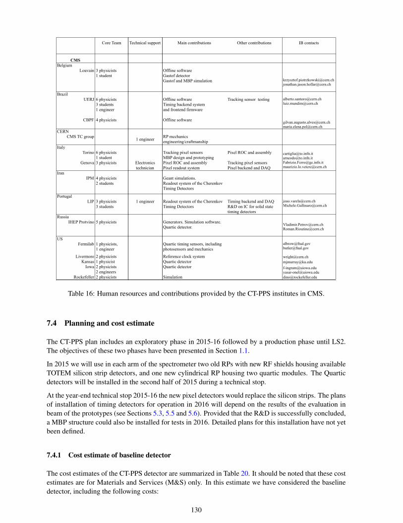
Core Team

CMSBelgium

Louvain 3 physicists 1 student

BrazilUERJ 6 physicists

3 students1 engineer

CBPF 4 physicists

CERNCMS TC group

ItalyTorino 6 physicists

1 studentGenova 3 physicists

IranIPM 4 physicists

2 students

PortugalLIP 3 physicists

3 students

RussiaIHEP Protvino 5 physicists

USFermilab 1 physicists,

1 engineer

Livermore 2 physicistsKansas 1 physicist

Iowa 2 physicists2 engineers

Rockefeller 2 physicists

Technical support

1 engineer

Electronics technician

1 engineer

Main contributions Other contributions IB contacts

Offline softwareGastof detectorGastof and MBP simulation [email protected]

[email protected]

Offline softwareTiming backend systemand frontend firmware

Tracking sensor testing [email protected]@cern.ch

Offline software [email protected]@cern.ch

RP mechanics engineering/craftmanship

Tracking pixel sensorsMBP design and prototyping

Pixel ROC and assembly [email protected]@to.infn.it

Pixel ROC and assemblyPixel readout system

Tracking pixel sensorsPixel backend and DAQ

[email protected]@cern.ch

Geant simulations.Readout system of the Cherenkov Timing Detectors

Readout system of the Cherenkov Timing Detectors

Timing backend and DAQR&D on IC for solid state timing detectors

[email protected]@cern.ch

Generators. Simulation software.Quartic detector. [email protected]

[email protected]

Quartic timing sensors, including photosensors and mechanics

[email protected]@fnal.gov

Reference clock system [email protected] detector [email protected] detector [email protected]

[email protected] [email protected]

Table 16: Human resources and contributions provided by the CT-PPS institutes in CMS.

7.4 Planning and cost estimate

The CT-PPS plan includes an exploratory phase in 2015-16 followed by a production phase until LS2.The objectives of these two phases have been presented in Section 1.1.

In 2015 we will use in each arm of the spectrometer two old RPs with new RF shields housing availableTOTEM silicon strip detectors, and one new cylindrical RP housing two quartic modules. The Quarticdetectors will be installed in the second half of 2015 during a technical stop.

At the year-end technical stop 2015-16 the new pixel detectors would replace the silicon strips. The plansof installation of timing detectors for operation in 2016 will depend on the results of the evaluation inbeam of the prototypes (see Sections 5.3, 5.5 and 5.6). Provided that the R&D is successfully concluded,a MBP structure could also be installed for tests in 2016. Detailed plans for this installation have not yetbeen defined.

7.4.1 Cost estimate of baseline detector

The cost estimates of the CT-PPS detector are summarized in Table 20. It should be noted that these costestimates are for Materials and Services (M&S) only. In this estimate we have considered the baselinedetector, including the following costs:

130

Core Team

TOTEM

CERN6 physicists, 1 engineer, 2 students

Czech RepublicPrague 2 physicists

Pilsen 3 engineers, 2 students

FinlandHelsinki 1 physicist,

2 students

Italy (INFN)Bari 4 physicists,

1 engineer, 2 students

Pisa/Siena 4 physicists, 2 engineers, 1 student

CollaborationCommonFund 2 engineers,

1 student

Technical support Main contributions Other contributions

RP Design, R&D, Interfaces to LHC, Operation, Edgeless Si Strip Tracking, Offline Software (in particular forward proton reconstruction), Physics Analysis, R&D Timing Detectors

Verification of movable beam pipe components. Timing systems.

Cooling.

Time reference, trigger and Readout Electronics.

Solid State Timing detectors. Physics Analysis.

Cabling infrastructure, Time reference (option Optical Fibers), Solid State Timing detectors, Readout and DAQ. Data analysis.

Cabling infrastructure, Time reference (option Optical Fibers), Solid State Timing detectors, Trigger electronics and firmware.

Offline Software (in particular detector simulation)

Electronics, Controls. Firmware

Table 17: Human resources and contributions provided by the CT-PPS institutes in TOTEM.

1. Final prototype or pre-production fabrication required to validate a final design or product quality,prior to production.

2. Engineering costs incurred during production at a vendor or contractor, not at a CMS and TOTEMmember Institution.

3. Production fabrication and construction costs, including quality assurance and system testing dur-ing the assembly process.

4. Transportation costs, integration and installation.

The TOTEM expenditure executed in 2013-14 on the Roman Pot project is summarized in Table 21. Itincludes:

1. The cost of the relocation to the 210m region of the 4 (out of 12) RPs used by CT-PPS trackingdetectors, as well as the cost of the new RF shielding;

2. The cost of two new cylindrical RPs for the CT-PPS timing detectors, including the movementsystem (motors and control), RP infrastructure (cables, cooling, vacuum, LV), and ferrites (fabri-cation, machining, bake out, cleaning).

131

Infrastructure RP MBPTracking sensors

Tracking readout

Timing sensors

Timing readout

Trigger & timing Offline SW

CMSBelgium

Louvain x x x

BrazilUERJ x x xCBPF x

CERNCMS TC group x x x

ItalyTorino x x x x

Genova x x xIran

IPM x x xPortugal

LIP x x x xRussia

IHEP Protvino x x

USFermilab x

Livermore xKansas

Iowa x xRockefeller x

TOTEM

CERN x x x x x x

Czech RepublicPrague x xPilsen x x

FinlandHelsinki x x

Italy (INFN)Bari x x x x

Pisa/Siena x x x xCollaboration

CommonFund x

Table 18: Summary of the participation of institutes in CT-PPS sub-projects.

These values include the costs of CERN services manpower. The manpower from the TOTEM collabo-ration having contributed to the project are not accounted for.

The TOTEM contributions to the silicon strip detectors to be used in 2015 and to the reference timingsystem are not included in the tables, neither the original cost of the four relocated RPs housing thetracking detectors.

In this chapter, all monetary values are expressed in CHF. The following conventional exchange rateshave been used to convert EUR and USD to CHF:1 USD = 1.0 CHF; 1 EUR = 1.2 CHF.

7.4.2 Objectives, plans and cost of R&D programme

Besides the construction of the baseline detectors, we propose to carry the R&D programme on MovableBeam Pipes and Timing Detectors described in Sections 3.6, 5.3, 5.5 and 5.6. In Table 19 we summarizethe physics motivations, objectives and time scale of the proposed R&D programme.

The results of the R&D programme will be evaluated in reviews to be carried out in the falls of 2015, 16and 17. These reviews will establish the basis for the decisions on the detector configuration to be usedin the following year(s).

We have estimated the cost of the development of prototypes of the new Timing Detectors and of proto-

132

types of Movable Beam Pipes (Table 22). Cost estimates of the construction of final versions of any ofthese items will be established after the evaluation of prototypes and the choice on the possible upgrades.

We have included in the Table 22 the cost of two additional cylindrical chambers, RP cylinder andferrites, integrated in present stations, to accommodate new timing detectors in 2016.

7.4.3 Expected funding and cost sharing

The global cost of the project is expected to be borne by all institutions participating in the project.Discussions with the Funding Agencies are ongoing to define the sharing of the total project cost.

133

Area

R&D(item

Phys

ics m

otiv

atio

nO

bjec

tives

Tim

e sc

ale

Tim

ing

dete

ctor

s with

tim

e re

solu

tion

of 1

0 ps

, with

m

ater

ial l

ess t

han

few

% n

ucle

ar in

tera

ctio

n, a

nd

with

hig

h gr

anul

arity

. Trig

ger s

yste

m b

ased

on

prot

on k

inem

atic

s.

Hig

h gr

anul

arity

Qua

rtic

Qua

rtic

bars

w/ 1

0 tim

es sm

alle

r cro

ss

sect

ion

allo

win

g to

redu

ce th

e do

uble

hit

indu

ced

inef

ficie

ncy

to a

neg

ligib

le le

vel.

Upg

rade

the

cent

ral 3

x3 m

m2 q

uartz

bar

s of t

he

base

line

dete

ctor

with

bar

s of ~

1mm

2 cro

ss se

ctio

n.

Stud

y of

opt

ical

wra

ppin

g an

d sm

all a

rea

SiPM

s.

R&

D c

oncl

uded

in

2015

Gastof'prototyp

esEx

celle

nt ti

me

reso

lutio

n an

d th

in m

ater

ial i

n th

e pr

oton

s pat

h. In

tend

ed fo

r use

in

asso

ciat

ion

with

hig

h gr

anul

arity

det

ecto

r ca

pabl

e to

add

mul

ti-hi

t dis

crim

inat

ion.

Bui

ld a

pro

toty

pe d

etec

tor f

or e

valu

atio

n in

test

be

am in

201

5. If

succ

essf

ul, b

uild

a se

cond

det

ecto

r fo

r ins

talla

tion

in 2

016

in b

oth

arm

s of P

PS.

R&

D c

oncl

uded

in

2015

Diam

ond'p

rototyp

es

Thin

and

fast

det

ecto

r tec

hnol

ogy.

Hig

h gr

anul

arity

requ

ired

for m

ulti-

hit

disc

rimin

atio

n. A

llow

s trig

ger s

yste

m b

ased

on

pro

ton

kine

mat

ics.

Eval

uate

pro

toty

pe d

etec

tors

and

fast

ele

ctro

nics

in

test

bea

ms.

Dem

onst

rate

resi

stan

ce to

100

fb-1.

Dem

onst

rate

hig

h ra

te c

apab

ility

.

R&

D c

oncl

uded

in

2016

/17

Timing'silicon'prototypes

Thin

and

fast

det

ecto

r tec

hnol

ogy.

Hig

h gr

anul

arity

requ

ired

for m

ulti-

hit

disc

rimin

atio

n. A

llow

s trig

ger s

yste

m b

ased

on

pro

ton

kine

mat

ics.

Eval

uate

pro

toty

pe d

etec

tors

and

fast

ele

ctro

nics

in

test

bea

ms.

Dem

onst

rate

resi

stan

ce to

100

fb-1.

Dem

onst

rate

hig

h ra

te c

apab

ility

.

R&

D c

oncl

uded

in

2016

/17

Trigger'integ

rated

'electronics

Trig

ger s

yste

m b

ased

on

prot

on k

inem

atic

s m

atch

ing

the

cent

ral s

yste

m a

llow

ing

to

redu

ce th

e ce

ntra

l trig

ger t

hres

hold

s.

Inte

grat

ed e

lect

roni

cs a

llow

ing

trigg

er b

ased

on

mm

2 gra

nula

rity

dete

ctor

.R

&D

con

clud

ed in

20

16/1

7

Beam

(pocketsMo

ving'B

eam'Pipes'prototyp

esB

eam

poc

ket w

ith lo

w R

F im

peda

nce.

Bui

ld a

MB

P pr

otot

ype

for i

nsta

llatio

n in

the

beam

du

ring

the

win

ter b

reak

of 2

015-

16.

R&

D c

oncl

uded

in

2016

/17

Timing(

detectors

Ulti

mat

e re

ject

ion

of p

ileup

bac

kgro

und

requ

ires t

ime

reso

lutio

n of

10

ps (f

acto

r 2

bette

r tha

n th

e Q

uarti

c ba

selin

e), c

ell s

ize

~1m

m2 c

lose

to th

e be

am (f

acto

r 10

smal

ler t

han

Qua

rtic

base

line)

, and

ele

ctro

nics

with

trig

ger c

apab

ilitie

s (o

verc

omin

g th

e lim

itatio

n im

pose

d by

the

trigg

erle

ss p

ixel

fron

tend

).

Table 19: Physics motivations, objectives and time scale of the proposed R&D programme.

134

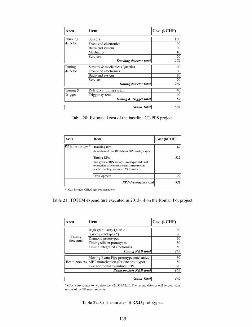
Area Item Cost (kCHF)

Sensors 150Front-end electronics 60Back-end system 30Mechanics 10Services 20

270

Sensors & mechanics (Quartic) 40Front-end electronics 60Back-end system 30Services 70

200

Reference timing system 40Trigger system 40

80

550Grand Total

Trackingdetector

Timingdetector

Timing & Trigger

Tracking detector total

Timing detector total

Timing & Trigger total

Table 20: Estimated cost of the baseline CT-PPS project.


Tracking RPs: 87Relocation of four RP stations. RP Faraday cages.

Timing RPs: 322Two cylinder RPs stations. Prototypse and final production. Movement system. Infrastructure (cables, cooling, vacuum, LV). Ferrites.

Development 29

438

*) Cost includes CERN services manpower

RP Infrastructure *)

RP Infrastructure total

Table 21: TOTEM expenditure executed in 2013-14 on the Roman Pot project.


High granularity Quartic 30Gastof prototypes *) 70Diamond prototypes 50Timing silicon prototypes 50Timing integrated electronics 50

250

Moving Beam Pipe prototype mechanics 30MBP motorization (for one prototype) 50Two additional cylindrical RPs 70

150

400

Beam pockets R&D total

Grand Total

Timing R&D total

Timing detectors

*) Cost corresponds to two detectors (2x 35 kCHF). The second detector will be built after results of the TB measurements

Beam pockets

Table 22: Cost estimates of R&D prototypes.

135

CMS-TOTEM Precision Proton Spectrometer Technical ...

Documents

Transcript of CMS-TOTEM Precision Proton Spectrometer Technical ...