Technological University Dublin Technological University Dublin

ARROW@TU Dublin ARROW@TU Dublin

Doctoral Science

2013-10

A Miniaturised Spectrometer Device for the Detection of Nitrogen A Miniaturised Spectrometer Device for the Detection of Nitrogen

Dioxide in an Urban Environment Dioxide in an Urban Environment

Brian Devine Technological University Dublin

Follow this and additional works at: https://arrow.tudublin.ie/sciendoc

Part of the Biomechanics Commons, Biotechnology Commons, and the Medical Biophysics Commons

Recommended Citation Recommended Citation Devine, B. (2013). A Miniaturised Spectrometer Device for the Detection of Nitrogen Dioxide in an Urban Environment. Doctoral Thesis. Technological University Dublin. doi:10.21427/D79594

This Theses, Ph.D is brought to you for free and open access by the Science at ARROW@TU Dublin. It has been accepted for inclusion in Doctoral by an authorized administrator of ARROW@TU Dublin. For more information, please contact arrow.admin@tudublin.ie, aisling.coyne@tudublin.ie.

This work is licensed under a Creative Commons Attribution-Noncommercial-Share Alike 4.0 License

A miniaturised spectrometer device for the

detection of Nitrogen Dioxide in an urban

environment

Brian Devine BSc.

A thesis submitted for the degree of Doctor of Philosophy to the Dublin

Institute of Technology

Supervisor

Dr. James Walsh

Biomedical and Environmental sensing laboratory

FOCAS institute

Dublin Institute of Technology

October 2013

i

Abstract

Monitoring of air pollutants, such as Nitrogen Dioxide (NO2), that are toxic or

environmentally damaging is a key metric for environmental protection agencies

worldwide. There is a constant need to develop new technologies and methodologies that

provide real-time, low cost pollution measurements over a broad range of sampling sites,

particularly in urban and industrial areas.

Typically, detection of pollutants in urban environments is performed using a

variety of techniques, many of which are expensive, require complex setups and are in

fixed locations. The novel system presented in this thesis is designed for portable, low cost

and in-situ detection of pollutants such as NO2 using Differential Optical Absorption

Spectroscopy (DOAS). The basis for the system is the new generation of miniature fibre

optic spectrometers that provide measurement specifications close to those of more

traditional high cost DOAS instruments which are used to cross calibrate the initial data.

The system can also be calibrated against other NO2 sampling techniques such as

chemiluminescence (CL) monitors. Based on laboratory calibration, the final measurement

accuracy of the system in the field was less than ± 0.5 ppb over a calibration dynamic range

of 0-50 ppb under typical daylight conditions. This level of accuracy was achieved with

repeated measurements, n=10, of custom made calibration cells containing known

concentrations of NO2.

Laboratory experiments using a controlled light source were designed to examine

the correlation between absorption and differential absorption using the NO2 calibration

cells with an algorithm based on the Beer-Lambert Law. These laboratory calibration tests

verified that differential absorption determined using the novel system can be used to

quantify NO2 concentrations both in the laboratory and in the open atmosphere of a

surrounding urban area. Field tests, using ambient sunlight as a source, were then

conducted and compared to concurrent CL measurements. Good correlations have been

confirmed between the novel-DOAS data and the established NO2 quantification methods.

Results prove that low cost spectrometer systems can be used to identify and quantify

gaseous pollutants in real-time using ambient sunlight.

ii

Declaration

I certify that this thesis which I now submit for examination for the award of PhD, is

entirely my own work and has not been taken from the work of others, save and to the

extent that such work has been cited and acknowledged within the text of my own work.

This thesis was prepared according to the regulations for postgraduate study by research of

the Dublin Institute of Technology and has not been submitted in whole or in part for

another award in any other third level institution.

The work reported on in this thesis conforms to the principles and requirements of the

DIT’s guidelines for ethics in research.

Signed______________________________ Date_________

iii

Acknowledgements

I would like to thank my friends and family for their continued support throughout this

project. I would especially like to thank Dr. James Walsh for choosing and guiding me

in my PhD. A special thanks also for Dr. Jack Treacy, Dave Byrne, Leonard Bolster, all

the researchers in the Biomedical and Environmental monitoring laboratory and the

staff and people of the FOCAS institute, DIT and the EPA.

iv

Contents

A miniaturised spectrometer device for the detection of Nitrogen Dioxide in an urban

environment........................................................................................................................ i

Abstract .............................................................................................................................. i

Declaration....................................................................................................................... ii

Acknowledgements ..........................................................................................................iii

Contents............................................................................................................................ iv

List of Figures ................................................................................................................... x

Chapter 1 Introduction ...................................................................................................... 1

1.1 Introduction 1

1.2 The Earth’s atmosphere 3

1.3 Transportation of pollution 8

1.4 Types of pollution and the health effects 9

1.5 Pollution chemistry 11

1.6 Photochemistry of NO2 in the atmosphere 12

1.7 Pollution regulations for NO2 14

1.8 Standard measurement techniques of atmospheric gases 16

1.9 Sampling and remote sensing methods for the detection of gas pollutants 20

1.9.1 Gas chromatography 20

v

1.9.2 Mass spectrometry 20

1.9.3 Particulate matter analysis 21

1.9.4 Chemiluminescence 22

1.9.5 Ultraviolet photometry 22

1.9.6 Ultraviolet fluorescence 23

1.9.7 Non-dispersive infra-red (ND-IR) spectroscopy 24

1.9.8 Differential optical absorption spectroscopy (DOAS) 24

1.10 Summary and thesis structure 26

CHAPTER 2 Differential Optical Absorption Spectroscopy ...................................... 28

2.1 Introduction 28

2.2 Light scattering effects 28

2.3 Determination of gas concentration by absorption 29

2.4 Beer-Lambert law 34

2.5 Differential absorption of NO2 40

2.6 Differential absorption coefficient α’ of NO2 43

2.7 History of differential optical absorption spectroscopy 45

2.8 Active and passive differential optical absorption spectroscopy 46

2.8.1 Active DOAS 47

2.8.2 Passive DOAS 49

2.9 Light scattering effects on the pathlength measured by DOAS instruments 50

vi

2.9.1 Atmospheric measurements with light scattering effects 52

2.9.2 Radiative transfer models, RTMs 54

2.9.3 Diurnal variation in slant column density 55

2.10 Summary 57

CHAPTER 3 Active and passive DOAS instrumentation for NO2 detection ............. 59

3.1 59

3.1Introduction 59

3.2 Current DOAS applications for NO2 detection 59

3.3 Satellite monitoring of NO2 65

3.4 Correlation spectroscopy using miniaturised spectrometers 69

3.5 DOAS software applications 70

3.6 Viewing geometry and the optical pathlength through the atmosphere 72

3.7 Meteorological and topographical influence on DOAS measurements 77

3.8 Cost analysis of commercial and mini-DOAS systems 79

3.9 Summary 80

CHAPTER 4 Materials and methods ........................................................................... 82

4.1 Introduction: Portable in-situ detection system 82

4.1.1 Instrumentation and sample requirements 82

4.2 Optical instrumentation 85

4.3 Optical alignment 89

vii

4.4 Miniaturised spectrometers and charge coupled devices 91

4.5 The back illuminated charge coupled device 95

4.6 Dark current and noise 97

4.7 Power and software requirements 99

4.8 Final setup for laboratory and field measurements 102

4.8.1 Sample preparation and measurements

102

4.8.2 Optical bench measurement procedures

103

4.8.3 Calibration

105

4.8.4 Urban measurement of NO2 with the novel-DOAS

108

4.9 Summary 111

CHAPTER 5 Comparison of chemiluminescence and DOAS for monitoring of NO2113

5.1 Introduction 113

5.2 Summary of literature for DOAS and CL comparisons 114

5.3 Dublin Institute of Technology DOAS monitor 115

5.4 Chemiluminescence instrumentation 119

5.5 Comparison of in-situ DOAS and CL 122

5.6 Experimental procedure with TCD-CL 124

viii

5.7 Analysis of the novel-DOAS with EPA-CL data 126

5.8 Summary 127

CHAPTER 6 RESULTS ............................................................................................ 129

6.1 Introduction 129

6.2 Laboratory setup and equipment tests 130

6.2.1 Initial laboratory tests

130

6.2.2 Laboratory tests

131

6.3 Laboratory tests using polypropylene bags 138

6.4 Laboratory tests with calibration cells 147

6.5 Comparison of each spectrometer for determination of differential absorption

150

6.6 Absorption and differential absorption determined using the USB4000 155

6.7 Initial measurements of the urban atmosphere to determine NO2 concentration

with the novel-DOAS 158

6.8 Calibration of the in-situ novel-DOAS instrument with calibration cells 163

6.9 Measurements of NO2 in urban environments and comparison to EPA-CL data

167

6.9.1 Correlation of novel-DOAS determined concentrations with EPA data

169

ix

6.9.2 Results of comparison of novel-DOAS with EPA chemiluminescence

175

6.9.3 Evaluation of CL and novel-DOAS data

181

6.9.4 Further analysis of the EPA and DOAS data comparisons

183

6.10 Summary 189

CHAPTER 7 Discussion and Conclusions ................................................................ 191

7.1 Project aims and background 191

7.2 Laboratory work and discussion of the results 192

7.3 Field work results 194

7.4 Summary of Conclusions 197

7.5 Future work 198

References: .................................................................................................................... 201

Appendix I Paper submitted for publication to the Atmospheric Measurement Techniques

1

Appendix II Matlab algorithm used for data analysis 1

Appendix II Conference Paper 2012 STRIVE 1

Appendix IV List of presentations & publications: 2

x

List of Figures

Figure 1.1 The vertical structure of the Earth's atmosphere, each layer is distinguished by

temperature, pressure and altitude above the Earth's surface[4] 4

Figure 1. 2 Planetary Boundary Layer (PBL): Illustration of the (a) Planetary Boundary Layer and

Urban Boundary layer (b) which has a height roughly that of the surrounding buildings.[5] 6

Figure 1. 3 Pollution monitoring zones A-D for the Republic of Ireland zone A covers Dublin city and

most of the surrounding urban area. Greater attention is given to this area because of the dense

population and activity. 18

Figure 1. 4 Annual mean NO2 concentrations at each zone 2002-2011 [17] 19

Figure 2.1. Extraterrestrial Sun spectrum (blue) and the spectrum of a 6000K blackbody radiator

(red). The features in the extraterrestrial spectrum are caused by the scattering and absorption of

the light at the surface of the Sun[7]. 30

Figure 2.2 Extraterrestrial (blue) Sun spectrum and direct (green) Sun spectrum [7] . Note the

attenuation of the spectrum especially in the infrared region 800 nm to 2500 nm 31

Figure 2.3 Solar Spectrum with Fraunhofer (FH) lines (measured with USB4000 spectrometer).

Significant FH lines between 360 nm and 400 nm, between 420 nm and 460 nm the most

significant FH line is near 435 nm. 32

Figure 2.4 (a) light transmitted from an emitter lamp to a receiver over a distance L with no absorber

(b) light attenuated (broken line) by the absorber. 35

Figure 2.5 Absorption profile of NO2 between 400 nm to 600 nm NO2 has prominent absorption

features in the visible region. This image was developed using a USB 4000 miniaturised

spectrometer. 38

Figure 2.6 Determination of the absorption using a single absorption feature at 440 nm detected by a

USB 4000 spectrometer 39

Figure 2.7 Comparison of reference (blue) and measured spectra (green). With labelled intensities of an

attenuated feature used in the determination of differential absorption D. 42

xi

Figure 2.8 Absorption Coefficients, α, data from literature sources Burrows 2000, Schneider 1987,

Vandaele, Burrows 1998, Bogumil 2003 cm2mol

-1 (x10

-19). The largest differences are between

Schneider data and the others as the data is much older and the resolution of the instrument used

was not as sophisticated as the others. [4] 44

Figure 2.9 OPSIS system emitter housing on the roof of DIT Cathal Brugha Street 48

Figure 2.10 Lower scattering altitudes of sunlight entering a DOAS receiver. Note the different

pathlength of the lower elevation angle as a result of scattering in the trace gas layer. [32] 51

Figure 2.11 Scattering altitudes of the light entering a DOAS receiver, the darker areas represent two

trace gas layers through which the light travels. The slanted path is represented by ds and the

vertical path by dz. [32] 54

Figure 2.12 Variation in slant column density for (a) NO2, (b) O3 for 20 May 2004 in Leicester in the

UK Leigh et al [58] from 4am to 10pm. The O3 has maximum column densities at night (see

text). During the day they mix with other molecules such as NO forming NO2 so their column

densities are near 0 during the day. 56

Figure 3.1 Monthly mean tropospheric column density of NO2 May 2013 obtained by GOME II

satellite[78]. The highest column densities have a red/pink colour. 69

Figure 3.2 MAX-DOAS under clear sky (a) and cloudy conditions (b). The clouds cause the light to

scatter resulting in variations in the optical pathlength of the light through the PBL and UBL

where NO2 concentrations are measured. [84] 75

Figure 3.3 Viewing geometry of the front end optics of the novel system. The determination of d,

pathlength, is found using the radius of the Earth, Re. 76

Figure 4.1 Optical fibres coupled to collimating lens aligned with each other on a bench. The bench

allows the adjustment of the emitting and receiving fibres for alignment on either side of the

polypropylene bag. 85

Figure 4.2 Transmission of light in optical fibre occurs as the light enters at the critical angle and

subsequently reflects off the cladding as it travels to the opposite end. 87

Figure 4.3 Schematic of how light rays passing through a sample are collimated by lenses and optical

fibres. 90

xii

Figure 4.4 Czerny Turner spectrometer design. The light enters at the aperture where the optical fibre

is coupled to the spectrometer. The light reflects off the opposite mirror onto the diffraction

grating, the diffracted light is then collimated by the second mirror and reflected onto the CCD

detector. 91

Figure 4.5 Structure of charge coupled device with three electrodes, a potential well is formed under

each electrode where the electronic charge is built up before conversion into an electronic signal.

93

Figure 4.6 Full frame transfer process of a CCD detector. The electronic signal builds up in the vertical

shift register and passed to the active area. From here it is transmitted to the horizontal register

followed by the amplifier. 95

Figure 4.7 A Back illuminated charge coupled device. Note thinned silicon layer where the spectral

etaloning is known to occur. 96

Figure 4.8 Raw intensity spectrum (a) of a tungsten light source used in the laboratory as a reference

measurement Io and an absorption spectrum (b) for NO2 with wavelength on the x-axes is between

300 nm and 700 nm. 101

Figure 4.9 Polypropylene bag placed in the path of a collimated light beam produced by a tungsten

source, optical fibres and collimating lenses, detected by a USB4000 detector. 104

Figure 4.10 Gas calibration cells. Each cell is 1.4 cm thick and each one is fitted with a stem for

placement in front of the detectors lens. 107

Figure 4.11 Schematic of the field apparatus of the novel-DOAS with the collimating tube and

adjustable aperture fixed to the collimating lens and fibre 110

Figure 5.1 Map of Dublin area that includes the paths of the DIT-DOAS system. Only the Cathal

Brugha street path is still available but it is nearly 2 km from Kevin Street and alignment is

difficult [105]. 116

Figure 5.2 Comparison of the data obtained from DIT-DOAS and EPA-CL instruments for 03-05-2001

118

Figure 5.3 Real-time data from the Rathmines monitoring station (25th

to 3rd

of October 2012). The NO

(green) O (blue) and SO (red) data are available from the EPA website [17] 119

xiii

Figure 5.4 CL monitor operation. Air is sampled at the inlet and the PMT measures light through NO

or NOx gases. NO2 is then found by subtraction. 120

Figure 6.1 Diagram of laboratory bench top setup as seen in chapter 4 131

Figure 6.2. Comparison of the dark current signal, a digital number, for one and 500 scans. The top

image is the dark current for 1 scan/ 10 ms and on the bottom image shows 500 scans/ 10 ms. Note

the improved signal to noise when more scans are averaged. 133

Figure 6.3 Variation in dark signal over time. The signal drops between the 7/7/11 (blue) and the

morning of the 8/7/11 (green) then rises above it (red) before rising again (cyan). The variation is

most likely due to the change in temperature of the spectrometer over time. 134

Figure 6.4 Optical setup of fibre optics with moveable stands on a rail without sample 135

Figure 6.5 Polypropylene (PP) bag sample positioned between the two collimating lenses on the optical

bench. Image is shown with the room lights on but measurements were taken in the dark to

remove a prominent peak at 435 nm produced by the room lights. 136

Figure 6.6 Hg peak detected by each spectrometer (left). The intensity on the y-axis is normalised

(right) to illustrate the resolution of each peak. The Maya2000 has broadening (404 nm to ~ 400

nm) not present in the USB spectrometers. 137

Figure 6.7 Spectral absorption data for four PP sample bags with different concentrations of NO2 and

one bag filled with air as a reference. The reference was used to determine the absorption spectra

of the four sample bags, figure 6.10. 138

Figure 6.8 Close up image of the raw intensity of an air-reference and NO2-Spectra. The red line

indicates the location of the feature used to determine D for each sample. D was also determined

for the air-reference to eliminate any error in the analysis. 140

Figure 6.9 Absorption spectra for the four different bag samples shown in figure 6.7. The absorption

feature at 440 nm was used to determine D. Each spectrum is normalised to 500 nm. 140

Figure 6.10 Absorption coefficient α (blue) for NO2 determined using a USB4000 miniaturised

spectrometer. A spectrum of the α obtained by Bogumil et al is shown for comparison[44]. 141

Figure 6.11 A and D, at 440 nm, determined from the intensity spectra in fig 6.8 and the results in fig

6.10. Note D is also shown for the air sample (zero concentration), this is only possible in the

laboratory but its illustration here helps demonstrate the effectiveness of the algorithm. 142

xiv

Figure 6.12 Comparison of 3 bags with approximately the same nominal concentration of (1900 µgm-3

)

144

Figure 6.13 Variation in A for different parts of sample bag the results show that the NO2 has a

uniform concentration throughout the bag after it is mixed. 146

Figure 6.14 Decrease in D (blue) and A (green), (440 nm) after 5 hours for one bag sample of NO2. The

correlation between D and A remains but the concentration is reduced by ~ 14% 147

Figure 6.15 Calibration cell between source (transmitting lens and fibre) and detector (receiving lens

and fibre) on the optical bench. The cells small size and stem allows precise alignment for each

test. 149

Figure 6.16 Absorption of each calibration cell using the USB4000 spectrometer Note the increase in

size of the absorption features for increasing concentration. 150

Figure 6.17 Results of A and D at 440 nm determined from USB2000 spectrometer results for each cell

sample. There is a good correlation between the two sets of results but D has larger error bars

than those for A. 151

Figure 6.18 Absorption at 440 nm for each cell using the Maya2000 (red) compared to the USB4000

(blue). The Maya2000 results shown are below the results from the USB4000 and USB2000 this is

likely caused by the BI-CCD of the Maya2000. 153

Figure 6.19 Alignment of the apparatus with a variable neutral density filter 154

Figure 6.20 Change in A (440 nm) compared to the percentage of the maximum signal (left image) as

the intensity (right image) is decreased by the NDF. The absorption (red) has a maximum

variation when the max % is below 20%. The signal to noise at this low intensity is very low at the

440 nm feature. 155

Figure 6.21 Correlation between A and D (440 nm) for each cell using the USB4000 spectrometer.

These results demonstrate the effectiveness of the algorithm and the accuracy of the technique.

DOAS data offset due to variation in chosen wavelengths. 156

Figure 6.22 Cell concentration and D (440 nm) for n=10 tests on each cell. This shows the good

repeatability of the measurements performed in the laboratory. 157

Figure 6.23 Novel-DOAS apparatus with camera stand. Close-up of collimating tube and 2m long

optical fibre with mini-spectrometer and laptop 159

xv

Figure 6.24(a) View from Cathal Brugha St. and (b) novel and commercial systems on Kevin St. roof.

Note path in (a) passes between the Spire and Central Bank. 160

Figure 6.25 Spectra of Xe lamp (red) and lamp and Sun (blue) between 430 to 500 nm obtained from

Cathal Brugha Street. 161

Figure 6.26 Solar spectrum with inset of 340 to 460 nm features recorded using the USB4000

spectrometer 162

Figure 6.27 Location of EPA monitor in Rathmines. The red circle highlights the inlet tubes for the

monitors. 163

Figure 6.28 Variation of concentration when PP bags are placed in front of the detector. The first point

on the graph represents the concentration without a bag. 164

Figure 6.29 Increasing D for 5 measurements (1) no-cell, (2) air-cell and each calibration cell (3-5)

containing NO2 with ambient sunlight as a source. The results show that the increase in

concentration from each subsequent sample results in an increase in absorption relative to the

difference in concentration. 165

Figure 6.30 Diurnal variation of D for the atmosphere (blue) and each cell over a period of 6 hours.

Note each NO2 cell has a consistently higher D than the no-cell and air-cell data. 167

Figure 6.31 Absorption of Sunlight with zenith reference measurement and α (x 2x105) determined by

Bogumil_2003. Although there are NO2 absorption features visible (at 440 nm) in the zenith

reference measurement (blue), this zenith spectrum will still contain traces of atmospheric NO2.

169

Figure 6.32 Variation of the concentration for NO2 in ppb for 26/05/11 (L~10 km) 170

Figure 6.33 Variation of D with a changing elevation angle θ. An increase in D when the USB4000 is

nearly parallel to the horizon suggests higher NO2 concentrations closer to the Earth’s surface.

171

Figure 6.34 Variation of D for different azimuthal directions the values for D range between 0.078 and

0.088. 172

Figure 6.35 Variation in concentration for zenith directed measurements. There is higher concentration

before 9am in the morning which can indicate high NO2 concentrations from chemical mixing at

twilight and morning rush hour traffic. 174

xvi

Figure 6.36 Variation in concentration for zenith directed measurements. As in figure 6.37 the data

shows a high value for concentration in the early hours of the day and slight rise in the evening.

174

Figure 6.37 Three day comparison of EPA-CL and novel-DOAS data. The estimated optical

pathlengths for the determination of the NO2 concentration for each day were L~6 km

respectively. 176

Figure 6.38 Concentrations of NO2 determined for four days. A single estimated pathlength of 6 km

was used. 177

Figure 6.39 Comparison of 3 days of DOAS and EPA-CL (L~10 km). For the all three days the NO2

concentration suggests a good correlation between the two methods. 178

Figure 6.40 Comparison of 4 days of DOAS and EPA-CL data. (Average pathlength L ~ 8 km) The 3rd

and 4th

of July are similar but small fluctuations in the DOAS data could be the result of

changeable weather conditions. 179

Figure 6.41 (a) Variation in NO2 concentration using DOAS (L~6, 20, 20, 6 km) 180

Figure 6.42 Change in NO2 concentration in ppb using two CL monitors for the weekend 29/07 to 02/08

of 2011 (90hrs=3/4days). The overall change in the data obtained by the two monitors show some

correlation which suggests that a CL monitor is capable of representing an average NO2

concentration in an urban area. 182

Figure 6.43 Data as shown in figure 6.45 but with the change in NO2 concentration determined by

DOAS (red) added. The estimated pathlengths for each day are L~ 6, 6, 10, 8 km respectively.

Heavy showers and dark cloud were also recorded for each day. 182

Figure 6.44 Comparison of in-situ DOAS (blue) and EPA-CL (red) for NO2 and data correlation 23-

25/07/11. The DOAS data is clearly not correlated well with the EPA-CL data. The slope of the

line in the scatter plot is large ~3.2 indicating a weak correlation between the two methods on

these 3 days. 184

Figure 6.45 Comparison of in-situ DOAS (blue) and EPA-CL (red) for NO2 and correlation 29/07/-

01/08/11 the slope of the line in the scatter plot is 1.3 which indicates a good correlation between

each set of data. 185

xvii

Figure 6.46 Comparison of in-situ DOAS (blue) and EPA-CL (red) for the concentration of NO2 and

correlation 28-30/09/11 the large difference on the third day (30/9/11) affects the data giving the

line on the scatter plot a slope of 5.4. 186

Figure 6.47 Comparison of the average EPA-CL and in-situ novel-DOAS data for 5 consecutive days

(L~10 km). There is a clear correlation between both sets of data obtained by the two different

methods. 187

Figure 6.48 Comparison of average CL and in-situ novel-DOAS for 4 days (L~ 6 km 10 km 10 km 6 km

respectively). Although there is some comparison in these results the variation in the estimated

pathlength determined by comparing the two sets of data suggests the results were not conclusive.

188

1

Chapter 1 Introduction

1.1 Introduction

Urban air pollution is a major worldwide concern, primarily because of the risks to

human health, which include damage to the human cardiovascular system from particulate

matter (PM) and damage to the respiratory system by chronic bronchitis, pulmonary

emphysema, lung cancer, asthma and other conditions [1]. Another major risk factor caused

by air pollutants is climate change. Green house gases, such as chlorofluorocarbons, trap

infra-red radiation in the Earth’s atmosphere causing increases in temperature. As a result

of the dangers from these pollutants, national and international regulations have been

developed for the monitoring and control of gas concentrations and emissions worldwide,

particularly in urban areas[2]. To understand the sources and monitoring of these pollutants,

we must have knowledge of the environment where the pollutants are and their interaction

with meteorological and natural conditions.

The objectives of the research presented in this thesis were to demonstrate that a

miniaturised spectrometer could be developed to measure the concentration of a gas in an

urban environment. The specific aims included developing a system that is inexpensive and

yet can be compared to current commercial and governmental monitoring systems. The

system should also be capable of determining spectroscopically the differential absorption

and hence the concentration of a gas without the need of a reference measurement.

2

The new system, identified as novel-DOAS, needs to be calibrated in the laboratory

and in the field. In the laboratory rigorous testing with custom made gas samples are used

to determine the accuracy of the analysis. Crucially, in the field, the system needs to be

comparable to the existing systems used for monitoring gas pollution by the environmental

protection authorities and the analysis of the data should be made in conjunction with data

provided by the literature and these authorities.

For this system, the focus will be on the detection of nitrogen dioxide (NO2) as it is

a common gas pollutant found in urban areas. As it is possible to detect NO2 in the visible

range of the electromagnetic spectrum and as it is also monitored continuously by the

Environmental Protection Agency (EPA) in the Republic of Ireland, it is an ideal analyte

for the development of an optical based system. It is produced by vehicle exhaust and other

forms of combustion. Chemiluminescence (CL) and differential optical absorption

spectroscopy (DOAS) monitoring systems are the standard method for detecting NO2 by

the EPA and were used for comparisons with the results obtained by the novel detection

system as it is the standard method for measuring NO2 concentrations in urban

environments. All the field measurements in this research were specific to Dublin city. It

will be shown in later chapters that CL was used for comparisons with the data collected by

the novel DOAS instrument proposed in this research as a result of the status of the larger

DIT-DOAS instrument that was already in place.

3

1.2 The Earth’s atmosphere

To simplify the structure of the Earth’s atmosphere, it is divided up into different

layers. The layers consist of complex structures divided up by their altitude and the

particular chemistry of each layer. The layers are illustrated in figure 1.1 [3].

Approximately 90% of the content of the Earth’s atmosphere is in the lower atmosphere,

see figure 1.1. The troposphere extends to approximately 10 km above the Earth’s surface

in the middle latitudes of the northern hemisphere. The layer above the troposphere, the

stratosphere, extends roughly 50 km above the surface. These two layers are separated by a

thin layer, known as the tropopause. It is in these two layers that anthropogenic pollution

enters the atmosphere. In the troposphere, the sources of the pollution derive from

industrial and domestic activities. The pollution detected in the stratosphere can result from

air traffic and the vertical transport of pollution due to chemical and physical processes.

4

Figure 1.1 The vertical structure of the Earth's atmosphere, each layer is

distinguished by temperature, pressure and altitude above the Earth's surface[4]

Close to the Earth’s surface, in the lower troposphere, there is a layer known as the

planetary boundary layer (PBL) which can reach a height of 1 km to 1.5 km [5]. Figure 1.1

shows how each layer is divided up by height and pressure. The figure also shows the

changing temperature gradient throughout the atmosphere. The pressure, temperature and

air mass in the atmosphere play a large role in the chemical reactions of gases in the

atmosphere. Temperature can affect the absorption cross section of a gas (discussed in

chapter 2) and the air mass can affect the transport of solar radiation (also in chapter 2)

through the atmosphere [6]. Major constituents of the atmosphere are listed in table 1.1.

The content of the air in the atmosphere is made up primarily of nitrogen and oxygen [1, 6].

In comparison, as much as 3% of the atmosphere can be made up of water which affects

5

humidity and the absorption of solar radiation [7]. Seen as an ideal gas, the air in the

atmosphere obeys the ideal gas law (equation 1.1), whereby the pressure and volume of an

atmosphere is directly proportional to its temperature[6].

nRTPV Equation 1.1

where p is the pressure in Pa, V is the volume in m3, and temperature T in Kelvin, though

units can vary for each. As figure 1.1 shows, there is a decrease in pressure with increasing

altitude because, as the force exerted by gravity is lower at higher altitudes, the density of

the atmosphere then decreases [1]. Other physical effects on the atmosphere include solar

radiation [7], the Earth’s temperature and the circulation of the atmosphere by wind and the

Earth’s rotation i.e. the Coriolis Effect [1].

Trace amounts of nitrous oxides (NOx) and other gases are present from gas phase

processes like the carbon and nitrogen cycles [1]. For NOx, there can be concentrations of

~1 pptv (part per trillion-volume) of NO2 and ~50 pptv of nitrogen oxide, NO. Besides the

naturally occurring trace gases, there are atmospheric constituents resulting from

anthropogenic (man-made) sources e.g. carbon monoxide, CO, and organic compounds like

Benzene.

6

Table 1.1 Substantial Constituents of the Earth’s atmosphere

Figure 1. 2 Planetary Boundary Layer (PBL): Illustration of the (a) Planetary

Boundary Layer and Urban Boundary layer (b) which has a height roughly that of the

surrounding buildings.[5]

Gas Chemical Formula Mixing Ratio volume (%)

Nitrogen N2 78.08

Oxygen O2 29.05

Argon Ar 0.93

Carbon Dioxide CO2 0.037

Water Vapour H2O 0.00001-3

Hydrogen H2 0.00005

Nitrous Oxide N2O 0.00003

7

As stated in section 1.1, the PBL is approximately 1km to 1.5km in height above the

Earth surface. The dimensions of the Urban boundary layer (UBL) can change depending

on the velocity of the atmosphere above the surface [8], as shown in figure 1.2. The UBL

can either resemble a large plume when the velocity is high, above 3 ms-1

, and a ‘dome’

above the urban area when velocities are less than 3 ms-1

.

In figure 1.2, the UBL that is close to the ground is where pollution levels are of

most interest [9], as the human activity responsible for the emission of pollutants is below

the 1-1.5km altitude and the major weather conditions that disperse the pollution occur

close to the ground e.g. wind, rain, humidity etc.. The height of the sampling monitors

used by environmental protection agencies is ~2 metres above ground [10] which covers

the height of human respiration and remote sensing monitors can be situated on rooftops

also within the UBL. Satellite monitoring of pollutant emissions are capable of tracking

ground column densities of pollutants but are not accurate when there is extensive cloud

cover in the line of site. The UBL can also be further divided up into the urban canopy

layer, which extends to the height of the buildings, the surface layer above this and the

mixed layer extending from the top of the surface layer to the boundary of the UBL and the

rest of the PBL [8]. The novel device developed for this research is a ground based remote

sensing system which should be capable of measuring the average NO2 concentration along

a path through the atmospheric layers close to the Earth’s surface. Therefore, knowledge of

the structure and dynamic nature of these layers is needed in the analysis of the recorded

data.

8

1.3 Transportation of pollution

For the measurements of pollutants in an urban environment, an understanding of

the atmospheric processes that transport pollutants and trace gases in the atmosphere is

needed, as the distribution of pollution is governed by whether the local atmosphere is

relatively calm or increasingly turbulent. An urban landscape can affect the transport of

pollution because of changes in building heights and the locations of pollution sources. The

scale and dimensions of street canyons are determined by the space between buildings in

the urban landscape and influence turbulence in the moving air between the buildings. The

magnitude of the turbulence in the atmosphere is then determined by the wind’s velocity

and direction [11, 12]. For traffic, the source of the pollution is dynamic and responsible for

diurnal variations in concentrations.

Thermal effects also play a role in the chemical reactions of the pollutants

particularly atmospheric inversions which are created by two weather fronts of different

temperatures meeting. These inversions can occur laterally and vertically. Inversions

mainly occur at night when the ground cools, gradually affecting the temperature at higher

altitude, and the lighter pollution rises as the cold air gets heavier. The pollution will meet

the inversion which can have the same temperature, preventing it from dispersing. This will

create higher concentration levels in one location [1]. As pollution rises it reaches a mixing

height, an altitude where a substantial amount of chemical mixing and dispersion occurs.

The height of this mixing layer will vary daily and seasonally as a result of changing

weather and topography [1]. Some pollutants are more susceptible to the photochemical

reactions, where sunlight can cause chemical reactions with pollutants such as Ozone, O3

and NO. As a result of the dynamic meteorological effects throughout the year, pollution

9

monitoring of an urban atmosphere is usually provided and correlated with the local

weather conditions.

1.4 Types of pollution and the health effects

Anthropogenic air pollution includes carbon oxides, sulphur oxides, nitrogen

oxides, ammonia, hydrocarbon compounds, oxidants and particulate matter [1]. Table 1.2

illustrates these different pollutants, the sources and dangers they present to human health

and the environment. As can be seen from the table, there are numerous sources of man-

made pollution, but not all pollutants are produced from these sources. They can be

produced from reactions with other chemicals or result from physical reactions with

sunlight, local temperature and even lightning.

10

Pollutant

Examples of

pollutants

Examples of

Sources

Risks to Human

Health

Carbon Oxides

CO,CO2

Fuel Combustion Cardio-vascular

damage

Nitrogen

Oxides, Nitric

acid

NO, NO2,

NO3, HNO2 Fuel Combustion

Respiratory cell

damage

Sulphur

Oxides,

Sulphuric acid

SO2, SO3,

H2SO4

Fossil fuels, smelting Respiratory/ irritant

Hydrogen

Compounds

NH3, HCN

Decomposition/Biom

ass burning Toxic, eye irritants

Hydro-carbons

PAH, VOC,

CH4

Gas phases of

petrochemicals

Various toxicity from

compounds

Oxides

O3

Photochemical

reactions w/ NOx,

etc.

Respiratory

Particulate

Matter

PM10, PM2.5

Burning, solid waste

disposal Respiratory visibility

Table 1.2 Typical anthropogenic pollutants: sources and the potential risks to human

health[1, 13]

Table 1.2 also shows that, for airborne pollutants, people with respiratory conditions

are the most at risk. The dangers of the pollutants include aggravation of conditions like

emphysema and asthma. Cardiovascular conditions can also be affected by compounds

capable of entering the blood stream through the lungs. The human eye is at risk from

exposure to larger particles in the atmosphere as well as some of the chemical compounds

like the hydrocarbon benzene [14, 15].

Detection methods will be described in more detail later in this chapter (section 1.9)

and subsequent chapters, but it is worth noting at this stage that several methods are

required to detect and monitor the different pollutants because of the characteristic

11

chemistry of each pollutant. For example, particulate matter may be detectable by optical

means, but for a chemical analysis of its constituents, a sampling method with chemical

analysis is more commonly used.

1.5 Pollution chemistry

Carbon oxides such as carbon monoxide and carbon dioxide are produced by the

combustion of fossil fuels and are particularly dangerous for human respiration. Carbon

Oxides are also green house gases which are responsible for the depletion of the Ozone

layer causing increases in the exposure of ultraviolet (UV) rays to humans.

Nitrogen oxides are also produced by combustion and can react with sunlight,

ozone, and hydrogen. Reactions between nitrogen and hydrogen create dangerous

chemicals such as ammonia, NH3 and the cyanide ion, CN- as well as nitric acid, HNO3.

Sulphur oxides are found in the atmosphere from combustion but also, like many other

pollutants, they are present due to natural reasons; for sulphur dioxide, SO2, volcanoes are a

large natural source. SO2 is one of three dangerous gases continuously monitored by the

environmental protection agency along with ozone, O3 and NO2, which will be examined in

more detail in the rest of this chapter and other chapters. NO2 is the dominant pollutant

used to demonstrate the effectiveness of the novel optical instrument described in this work.

Hydrogen can react with carbon and oxygen in a vast number of ways, producing a

large range of organic compounds like alcohols, aldehydes and organic acids [1], some of

which are collectively known as volatile organic compounds (VOCs) as they can easily be

vaporised. These VOCs include solvents like benzene, which can form the basic structure

behind more complex hydrocarbons known as polycyclic-aromatic-hydrocarbons (PAHs),

12

for example Benzene (C6H6) based PAHs which are in solid form under atmospheric

conditions [1].

Also of interest for pollution monitoring is particulate matter or PM. Like the others

mentioned, their presence in the air is from combustion but also from chemical reactions.

The particulates can occur by anthropogenic activities like construction where large

amounts of fine dust is produced and natural sources like plants, micro-organisms and

ocean spray [1]. PM of <20 µm are also known as aerosols, because the particles are

suspended in the atmosphere. Aerosols produced from chemical reactions include nitrate

aerosols formed from the oxidation of nitrogen oxides, as a result of this the monitoring of

these aerosol concentrations can be linked to the concentrations of nitrogen compounds e.g.

NO2 [16]. PM sampling instruments usually sample particle sizes of PM10 and PM2.5 (10

µm and 2.5 µm).

1.6 Photochemistry of NO2 in the atmosphere

As NO2 is the pollutant of interest in this work, it is looked at in more detail in the

following sections. The concentration of NO2 is affected by the concentrations of other

nitrous oxide gases, ozone and sunlight. O3 concentrations are monitored at low altitudes

for the risks they can pose to humans and there is some correlation between the O3

concentrations and NO2 concentrations because of the chemical reactions (Reactions 1.1-

3)[1].

13

NO + O3 → NO2 + O2 (Reaction 1.1)

The O2 in this reaction is a free radical molecule that has one unpaired electron and

like NO will rapidly react when exposed to other molecules in the atmosphere. NO can be

produced by photochemical reaction when light is absorbed by the molecule as in (reaction

1.2). Equation 1.2 describes the relationship between the energy needed for the reaction and

the wavelength λ. For NO2 reactions are more likely to take place at wavelengths between

UV and 420 nm because light in this region has a higher energy.

E =hc/λ Equation 1.2

NO2 absorbs light in the wavelength region of 350 nm to 500 nm, which is largely blue,

which is why it appears as a red brown colour [1].

NO2 + hν → NO + O (Reaction 1.2)

The Oxygen formed by dissociation in (reaction 1.1) will undergo further reactions to form

O3, (reaction 1.3), where M is a molecule that accepts excess energy from the reaction e.g.

N2 [16].

O + O2+M→O3+M (Reaction 1.3)

The Oxygen produced from (reaction 1.2) will react to form several photochemical

products including NOx, peroxy acetyl nitrates (PAN) and O3. The free radicals will have

low concentrations and short residence times in the atmosphere because of the high

reactivity of these molecules.

Other photochemical effects are caused by aerosols and large air molecules which

cause photons to scatter as they travel through the atmosphere. Large aerosol particles of

14

sizes ranging from 0.4 µm to 0.7 µm are largely responsible for Mie scattering where light

radiation with wavelengths of the same size is scattered. This scattering can affect visibility

as a haze. The air particles with sizes of 0.03 µm are responsible for Rayleigh scattering.

The small size of the molecules results in scattering of wavelengths of light in the visible

region and is the reason for the blue colour of the sky[1] whereas the red sky at twilight is

caused by scattering at a much longer pathlength as the Sun appears to set [16]. Another

form of scattering is Raman scattering, whereby there is an energy transfer between the

scattering molecule and the incident photons. Raman scattering can have an effect on the

solar spectrum of ambient sunlight which is used to measure pollution concentration. The

processes of scattering and absorption are described in more detail in chapter two as they

largely influence the appearance of absorption spectra of the atmosphere.

1.7 Pollution regulations for NO2

The needs to scientifically quantify the concentrations and emissions of pollutants

are outlined in the international and national regulations such as those developed by the EU

[9] and the Irish government[17]. The Irish government environmental protection agency

(EPA) is responsible for all monitoring, licensing, reporting and policy development in the

area of the natural and urban environment of the Republic of Ireland under the Protection of

the Environment Act 2003 [15]. The agency is also responsible for the enforcement of

environmental regulations. The limits for the average and annual maximum concentrations

and emissions are set by the EU. Targets are to be met by each union member within a

designated period of time and failure to meet these targets can result in penalties. The EPA

15

is responsible for the continuous monitoring of pollutants to ensure that these targets are

met.

Assessment

Hourly limit value for

the protection of

human health(NO2)

Annual limit for the

protection of human

health (NO2)

Annual critical level

for the protection of

natural

ecosystems(NOx)

Upper assessment

threshold

140 µgm-3

, not to be

exceeded more than 18

times a year

32 µgm-3

/17 ppb

24 µgm-3

/ 12.8 ppb

Lower assessment

threshold

100 µgm-3

, not to be

exceeded more than 18

times a year

26 µgm-3

/ 13.8 ppb

19.5 µgm-3

/ 10.4 ppb

Table 1.3 Article 35 Annex II of the Clean Air for Europe (CAFÉ) directive. The

thresholds for NOx and NO2 established from 01-01-2010.

The EU directives outlined for NO2 concentrations in ambient air quality assessments state

the upper and lower thresholds for concentrations that were to be met by 2010 and are as

shown in table 1.3. Annex VI of the CAFÉ [9]document describes the measurement

methods for different pollutants. The document also outlines the long term objectives for

monitoring, concentration limits for the protection of human health and the alert thresholds

e.g. NO2 - 400 µgm-3

and SO2 – 500 µgm-3

. For human health it is recommended that the

levels of NO2 should not exceed 200µgm-3

(106.4 ppb) in one hour more than 18 times

/year and 40µgm-3

for a calendar year. In contrast, the limit for benzene is 5µgm-3

in a

calendar year.

16

1.8 Standard measurement techniques of atmospheric gases

To ensure the regulations are met, the recommended measurement methods for

different pollutants can be divided up into categories where samples are extracted and

examined separately, in-situ monitoring and remote sensing techniques. Each technique can

involve instruments that are based on the same scientific method e.g. infra-red spectroscopy

for separate examination and remote sensing. But the method chosen can be related to the

chemical analyte being measured, instrument cost, location, accuracy and specifics of the

measurement. The specifics of the measurement refer to measurements where sample

examination is more accurately performed with a specific procedure such as sample

extraction for further analysis as in the measurement of particulate matter or remote sensing

when a large area needs to be monitored.

European Standard methods for different pollutants are listed below in table 1.4.

The measurement techniques include sampling and remote sensing methods. The sampling

methods include gas chromatography, mass spectrometry, chemiluminescence (CL) and

UV photometry. The remote sensing techniques which are predominantly spectroscopic

techniques include UV fluorescence, Fourier transform infra-red spectroscopy (FTIR) and

DOAS. There are other techniques such as DIAL (Differential Absorption Light Detection

And Ranging) and atomic absorption spectroscopy (table 1.2) that can be used for sample

analysis but the methods listed in table 1.4 are designated as the standards by the European

Union [9]. DOAS is not considered the primary standard for NO2 measurement but it is

popular as it can simultaneously measure several analytes accurately over a large

geographical area[13].

17

Pollutant Compound Principles of reference method

SO2 UV Fluorescence

NOx Chemiluminescence/Differential Optical Absorption Spectroscopy

CO Non-dispersive Infrared (IR) Spectroscopy

O3 UV Photometry

Benzene PM10 with fluorescence/gas chromatography/mass spectrometry

PM2.5, PM10 PM reference sampler

Other Heavy Metals (Ni, Cd) PM10 mass spectrometry

Table 1.4 Pollutant Compounds and the standard methods employed to monitor

concentrations of each one. [18]

The EPA in Ireland monitors several pollutant gases including CO, SO2, O3 and NOx gases.

The concentration levels of these gases are monitored by UV-photometry (tropospheric

ozone), UV-fluorescence (SO2), non-dispersive IR (CO) and CL (NOx) [9] (see chapter 1).

For monitoring, the country is divided up into four geographic zones, see figure 5.1, with

Dublin and Cork cities representing zones A and B, and zones C and D representing 21

large towns and the rest of the country respectively [19].

18

Figure 1. 3 Pollution monitoring zones A-D for the Republic of Ireland zone A covers

Dublin city and most of the surrounding urban area. Greater attention is given to this

area because of the dense population and activity.

Annual concentrations of pollutants are published by the EPA and are available on

the EPA website (www.epa.ie/air/quality/data/rm/gas/) where they are frequently updated.

Figure 1.3 [20] shows the annual NO2 results from individual zones from 2002 to 2011. As

would be expected, the concentrations are much greater in the Dublin city zone, followed

by Cork in zone B, because of larger traffic congestion and the concentration of population

and industry compared to zones C and D.

19

Figure 1. 4 Annual mean NO2 concentrations at each zone 2002-2011 [17]

To monitor NO2, CL detectors are located in several locations, in Dublin, including

Dun Laoghaire and Rathmines on the outskirts of the city centre and Coleraine St. and

Winetavern St. in the city centre itself. The higher concentrations of NO2 in Dublin city

make it ideal for calibration of the novel system within the Republic of Ireland. Figure 1.4

shows how the data is presented daily by the EPA and past data is also available from the

EPA website, both of which make it possible to compare measurements taken with the

novel system to determine if the data shows any correlation.

20

1.9 Sampling and remote sensing methods for the detection of

gas pollutants

In the following examples, the methods employed for detecting pollution by

environmental agencies are described with particular attention given to methods used to

measure concentrations using samples and remote sensing. Some detail is given into the

methods employed to detect NO2, specifically CL and DOAS, but these will be examined

in more detail in the remaining chapters. Chapter 5 will describe how these two methods

can be used to determine how well the results of each are correlated.

1.9.1 Gas chromatography

This technique involves the separation of the gas sample for identification[21]. It

requires the concentrations of the compounds constituents being proportional to each other

when separated by a mobile gaseous phase and a stationary phase. The output is usually

combined with mass spectrometry. The method is complex but is very sensitive and can be

used for a variety of compounds e.g. SO2 and organic compounds.

1.9.2 Mass spectrometry

Mass spectrometry involves the separation of a sample into its mass-charge ratio.

The sample is ionized and the separation is performed using an electromagnetic field

21

through which the ionized beam is directed. The electromagnetic field is produced by a

magnet which splits the beam into different masses that are detected separately and

identified when each ion signal is processed into a mass spectrum. The mass charge ratio is

described in Equation 1.3.

aBEQ

M/)*( Equation 1.3

The mass-charge ratio M/Q (kg/C) is proportional to the electric field (V/m) and the

magnetic field (T) vector product, E and v*B respectively, and is inversely proportional to

the acceleration (m/s2),a, of the beam. Mass spectrometry is a powerfully sensitive

technique for the identification of a sample. It is performed in the laboratory to determine

particulate matter constituents, organic molecules and heavy metals. It is often performed

with gas chromatography, GC-MS[22].

1.9.3 Particulate matter analysis

Particulate matter (PM) is monitored using a Tapered Element Oscillating

Microbalance or TEOM[23], in which a sample is extracted through an inlet and filtered.

The filter is weighed before and after extraction and the PM is identified by gravimetric

means i.e. the weight difference before and after extraction. The concentration is the total

PM divided by the air volume. The different size particulate matter PM2.5 and PM10 can be

monitored separately with PM10 monitors used for the detection of large molecules such as

organic molecule as well as heavy metals like Lead and Nickel. The methods used to

22

identify the extracted samples may vary from a combined technique such as gas

chromatography mass spectrometry (GCMS) to spectroscopic analysis.

1.9.4 Chemiluminescence

Measurements using CL are made using an air sample extracted through an inlet

which then reacts with a molybdenum catalytic converter[24]. Light is passed through the

gas and the intensity is measured by a photomultiplier tube (PMT). The concentrations of

NOx and NO are determined separately and the NO2 concentration is then found by the

subtraction of these two. CL detectors have very good sensitivity but are usually used for

NOx measurements only. They are the standard method used by the Irish EPA for nitrogen

oxides, a further analysis and more detailed description of CL operation is given in chapter

5.

1.9.5 Ultraviolet photometry

Ozone can be measured with several different techniques including CL [13], DOAS

and UV-photometry. UV-Photometry involves the detection of monochromatic light in the

UV range passing through a sample and received by a detector. Photometry and

spectroscopy involve the measurement of light. Spectroscopy specifically measures the

wavelength/frequency of light from absorption and scattering processes caused by its

interaction with molecules. Photometry measures the light intensity from chemical and

electrochemical reactions such as the measurement of flames intensity when the sample is

combusted. The analysis is performed using the Beer-Lambert law (see chapter 2) which

23

determines the concentration by comparing the amount of light absorbed with the total light

emitted taking into account the length of the cell. The exact mathematical description will

be explained in more detail in the next chapter as it is used for DOAS. The gas temperature,

pressure are usually recorded simultaneously [25]. Measurements of O3 by the EPA record

the concentrations in µgm-3

but O3 measurements are also performed using remote sensing

methods where Dobson units (molecules cm-3

) are used [26].

1.9.6 Ultraviolet fluorescence

UV fluorescence is used in the detection of sulphur dioxide[21]. The method is

based on the principle of fluorescence, whereby light of high energy (UV) is absorbed and

after undergoing electronic and vibrational transitions (chapter 2) at high energy levels it

emits light of longer wavelengths (visible) as it returns to lower energy levels. The emitted

radiation is then detected and used to determine sample concentration. In practice, a light

from a single source can be absorbed and the emitted light, consisting of several

wavelengths, can be directed through an emission monochromator before reaching the

detector. In practice, it is ideal for the detection of species with small molecular cross

sections such as free radicals[6]. For pollution monitoring, it is the standard method for the

detection of sulphur dioxide.

24

1.9.7 Non-dispersive infra-red (ND-IR) spectroscopy

Carbon Monoxide can be detected in the longer wavelengths of the infra-red region

of the electromagnetic spectrum. For ND-IR spectroscopy, a broadband IR beam is emitted

by a heated coil. The beam passes through a glass filter wheel and is split into two beams.

One beam passes through a measure cell of nitrogen gas and the other passes through a

reference cell with a mixture of CO and N2. The sample cell with the CO folds the light

beam giving it an effective absorption path length of up to 16 m [27]. Upon exiting the

sample cell, the beam travels through a band-pass filter cell which narrows the beam to

wavelengths where the CO would have absorbed the most. A detector then receives the

beams from the measure and sample cells and converts the light signals into voltages which

represent the different intensities. Software is used to represent the intensity as a spectrum

where different features can be identified at different wavelengths or frequencies. The

differences in the two intensities at wavelengths where CO is known to absorb light are

used to determine the CO concentration.

1.9.8 Differential optical absorption spectroscopy (DOAS)

Like ND-IR, DOAS is primarily a spectroscopic technique[13]. The operation of the

instrument is based on the principle of light received by a detector being absorbed at

specific wavelengths. These wavelengths can then be used to identify the components of

the medium through which the light has passed. The amount of light absorbed is

determined by the ratio of the intensity of the emitted light without any absorber present to

25

the intensity of the light received after it has passed through the absorber. For differential

absorption, the original light intensity before absorption is not known, so a differential

absorption is determined mathematically using the attenuated features in the raw intensity

spectrum. If the path distance the light takes through the absorber and the wavelengths of

the attenuated features in the measured spectrum are known, the concentration of the

absorber can be determined. The DOAS technique, described in more detail in chapter 2,

involves the detection of a broadband light beam from a source or emitter by a receiver.

The receiver converts the light into an electrical signal. The broadband signal is then

analysed mathematically by the systems software. The commercial systems determine

concentrations of several gases including SO2, NO2, O3[28] and volatile organic

compounds (VOCs).

It is worth mentioning other optical methods used to determine the concentrations

of gases in the atmosphere, such as LIDAR (LIght Detection And Ranging), photoacoustic

spectroscopy and cavity enhanced absorption spectroscopy. These techniques are effective

and accurate but do require light sources that are stable and coherent. The photoacoustic

and cavity enhanced methods in particular are performed with collected samples rather than

by remote sensing [29], [30, 31]. Individual wavelengths of the signal can also be analysed

separately to determine the concentration of one analyte.

The DOAS method can also be applied in numerous ways for the remote sensing of

pollutant concentrations where no fixed source is used [32]. In these setups, the pathlength

is not always known, so the data is measured as a column density e.g. m2/kg. DOAS is the

main method used for this research and is described in further detail in the next two

chapters. The novel-DOAS device proposed in this research will be designed and

26

constructed to measure NO2 using relatively inexpensive equipment and a specially

designed algorithm for calculating the differential absorption.

1.10 Summary and thesis structure

The detection of pollution in the atmosphere has become vital in the last 100 yrs as

it has been identified as a danger to human health, the environment and the atmosphere. Of

particular danger to human health is pollution in the lower troposphere, especially the urban

boundary layer because of its proximity to dense urban structures and constant commercial,

domestic and industrial activity. The consequences of increased anthropogenic pollution in

the lower atmosphere include increasing respiratory, pulmonary and cellular damage to

humans.

As well as the chemicals released into the atmosphere, there are several chemical

and photochemical reactions that produce dangerous molecules e.g. NO reaction with water

producing nitric acid which can fall as acid rain under specific meteorological conditions.

Regulations to monitor pollution are outlined by the European Union and the Irish

Government and the monitoring is performed by the Environmental Protection Agency.

Several techniques are employed in the detection of pollutants depending on the type of

molecules, size of particulate matter and specific wavelength absorption.

In this thesis, the monitoring of pollutant NO2 by a novel-DOAS system will be

examined. Particular attention will be given to the differences between Passive and Active

DOAS. As the portable novel-DOAS system being described is designed to use ambient

sunlight (Passive system) the difficulties and advantages this approach will be described in

27

detail. The history and development of DOAS will be described in chapter 2, as well as the

mathematical derivation of the Beer-Lambert law and the effects of light scattering on the

atmospheric measurement.

Chapter 3 describes current commercially available DOAS instrumentation as well

as descriptions of the software applications, viewing geometry, meteorological aspects and

the comparative instruments used in Passive DOAS. Chapter 4 describes the equipment and

rigorous setups employed for the laboratory and atmospheric measurements that were

performed. Chapter 5 pays particular attention to how Passive DOAS compares to CL, the

standard technique for NO2 monitoring employed by the EPA. The methods used to

compare the portable system to the local CL system are also described.

The results of the laboratory and field measurements in chapter 6 demonstrate the

effectiveness of the determination of the differential absorption by analysis of the

atmospheric spectra. The laboratory results will show how well the differential absorption

compares to absorption determined with a reference measurement and the field data will

illustrate how the system can be calibrated outside the lab and how comparisons of CL data

recorded by the EPA can be achieved.

28

CHAPTER 2 Differential Optical Absorption Spectroscopy

2.1 Introduction

In this chapter, closer attention is given to differential optical absorption

spectroscopy (DOAS). A description is given of how the concentration of an analyte such

as NO2 is measured using the absorbed light along a fixed pathlength. The mathematical

determination of gas concentration is performed in DOAS by the Beer-Lambert Law which

requires a constant known as the absorption coefficient.

The absorption coefficient for NO2 can be known for a range of wavelengths but,

for the analysis method used in this thesis, a single value for a range of wavelengths is

required and a description is provided here on how that value is obtained.

An analysis is also provided of the theory behind the two forms of DOAS

measurements that can be achieved with and without a fixed light source and a known

pathlength.

2.2 Light scattering effects

Measuring a gas using absorption spectroscopy requires an understanding of the

physical processes that affect electromagnetic radiation, light, as it travels through an

analyte. The interaction of light with the atmosphere is typically described as extinction

29

processes. Extinction can occur in three different ways, from elastic scattering of the light,

inelastic scattering and absorption [12]. Elastic scattering occurs when a photon collides

with a molecule in the atmosphere and is scattered away from it. The energy of this

scattered photon is equal to the energy of the incident photon before the interaction. There

are two types of elastic scattering: Rayleigh scattering where the scattering particles are of a

relatively small size compared to the wavelength of light, for example molecules of N2 and

O2. Larger particles such as those found in particulate matter (PM) cause the type of elastic

scattering known as Mie scattering.

Inelastic scattering is caused by a photon colliding with a molecule where a fraction

of its energy is lost as it is transferred to the molecule. The molecule may also transfer a

portion of its energy to the photon. Raman scattering is inelastic scattering where the

scattering particle is smaller than the wavelengths of the incident and scattered light.

Raman scattering can be explained in quantum mechanical terms as occurring as rotational

when the angular momentum, J, of the particle is affected by the interaction and vibrational

when its harmonic oscillation is affected[6]. The vibrational Raman scattering is the weaker

of the two forms of Raman scattering.

2.3 Determination of gas concentration by absorption

Joseph von Fraunhofer was the first to observe dark absorption lines in solar spectra

using spectroscopic gratings[33]. These lines where later identified as the absorption of

light at different wavelengths in the Sun’s atmosphere. Figure 2.1 shows the spectrum of a

6000 K black body radiator (red) compared to the extraterrestrial solar spectrum (blue) and

30

figures 2.2 shows the difference between the extraterrestrial solar spectrum (blue) and a

direct spectrum (green). These images are from a DIT Matlab file developed from data

found in the Simple Solar Spectral Model for Irradiance [7].

Direct solar radiation occurs when the sunlight is perpendicular to the Earth’s

surface. Indirect, diffuse solar radiation is sunlight scattered by clouds, PM and water

vapour. Indirect scattering is responsible for daylight, even on overcast days, but the path

the light travels through the atmosphere can vary depending on the atmospheric conditions

[34].

Figure 2.1. Extraterrestrial Sun spectrum (blue) and the spectrum of a 6000K

blackbody radiator (red). The features in the extraterrestrial spectrum are caused by

the scattering and absorption of the light at the surface of the Sun[7].

31

Figure 2.2 Extraterrestrial (blue) Sun spectrum and direct (green) Sun spectrum [7] .

Note the attenuation of the spectrum especially in the infrared region 800 nm to 2500

nm

As figures 2.1 and 2.2 show, Fraunhofer features are abundant throughout the solar

spectrum and must be taken into account when a measurement of atmospheric pollutants is

determined using wavelength dependent variables. Figure 2.3 shows dominant Fraunhofer

lines between 340 nm and 460 nm. The letters N, L, K, H, e and G are the alphabetical

labels of the Fraunhofer lines used represent the elements iron, Fe (letters N, L and e),

calcium, Ca, (K) and nickel, Ni which cause absorption at each wavelength [35]. Figure 2.3

shows both the alphabetical designation and the chemical symbol for significant lines

between 340 nm and 460 nm.

32

Figure 2.3 Solar Spectrum with Fraunhofer (FH) lines (measured with USB4000

spectrometer). Significant FH lines between 360 nm and 400 nm, between 420 nm and

460 nm the most significant FH line is near 435 nm.

An effect of Fraunhofer lines is the “Ring” effect which is most likely caused by

rotational Raman scattering, whereby the angular momentum of the molecules in the

atmosphere are affected by collisions which can cause changes in the wavelengths of

Fraunhofer lines depending on the molecules with which the incident light interacts [36-

38]. The effect can also be described as a “filling in” of the Fraunhofer features in direct

sunlight more than those in indirect sunlight and can be seen as the features appear deeper

or more skewed than features with little influence from the Ring effect. The effect can be

33

approximated using a spectrum which is the reciprocal of a reference direct sun spectrum

taken at noon or as a fraction, as in equation 2.1.

elasticinelasticring III / Equation 2.1

The Ring effect is of concern when spectral analysis is made of a broad spectral

range, but can be minimised when only a few wavelengths are used for the analysis, as

absorption features can be chosen that have no or negligible interference from Fraunhofer

lines but are still known to show absorption features of atmospheric gas under

investigation.

The absorption of a photon by a molecule differs from the scattering effects as the

number of photons changes after the collision. An absorber such as NO2 will absorb colours

in the visible range of wavelengths, except the longer wavelengths which is why it has a

brown reddish colour. The energy is mathematically related to the wavelength of the

incident and emitted light by equation 2.2 (equation 1.2 chapter1).

E=hc/ Equation 2.2

where the speed of light, (italic c), in ms-1

is equal to the product of the lights wavelength,

(λ), in nm and the frequency (f), in Hz.

c=f Equation 2.3

The intensity of incident light on a medium where light is absorbed can be attenuated by

the medium at certain wavelengths that can be used to identify the absorber.

34

2.4 Beer-Lambert law

The transmission of light through an absorbing medium is proportional to the ratio

of the intensity of light before it passes through the medium to the light after it is absorbed,

see equation 2.4. Where ε is the molar absorptivity (m2/mol) and N (cm

-3) is the number

density of the specific absorber under investigation.

NLIIT 01010 /loglog Equation 2.4

Log10T is also commonly referred to as the Optical Density. Alternatively, the Lambert-

Beer law is commonly expressed as.

lnT = -L Equation 2.5

where is the absorption co-efficient of the material, in units of cm-1

. can also be

expressed in terms of the number density of absorbing species per unit volume, N (cm-3

) as

= σN, where is the absorption cross section per species, in units of cm-2

. Relating

equations 2.4 and 2.5, c=log10e = Nlog10e. Thus [39].

lnT = -NLlog10e Equation 2.6

According to Beer’s law, the absorber concentration is directly proportional to the

absorption which is also proportional to the ratio of the incident light and the transmitted

light at wavelengths λ[13]. In equation 2.7, Io (λ) represents the light incident on the

absorber and I (λ) the attenuated light, the fraction of Io/I is directly proportional to c.

35

NI

Io

)(

)(

Equation 2.7

J.H. Lambert showed that the fraction of transmitted light and light collected is also

proportional to the thickness of the absorber[6], or more specifically, the path taken by the

light through the absorber as shown in equation 2.8. Figure 2.4 illustrates the light

transmitted from an emitter (lamp) to receiving optics and detector with no absorber (a),

and the light transmitted through an absorber in (b). The light attenuated by the absorber in

(b) is illustrated by the broken line.

Figure 2.4 (a) light transmitted from an emitter lamp to a receiver over a distance L

with no absorber (b) light attenuated (broken line) by the absorber.

LI

Io

)(

)(

Equation 2.8

The absorption of the light (A) by the absorber is determined mathematically as the

natural logarithm of the fraction of light emitted Io (λ) to the light absorbed I (λ) because

36

the attenuation of the beam of light by the absorber over the pathlength L is decreased

exponentially.

))(

)(ln()(

0

I

IA Equation 2.9

Taken together equations 2.7 to 2.8 show that the total absorption is directly proportional to

the product of concentration of the absorber and the pathlength traversed by emitted light

towards the receiver, equation 2.10.

NLI

IoA )

)(

)(ln()(

Equation 2.10

To determine the concentration of a gas absorber for more than one wavelength,

over pathlength L, the nature of the absorbing medium and the characteristic absorption

cross section, σ() at specific wavelengths, needs to be known. For measurements of gas

pollution, the absorption cross section represents the characteristic absorption profile of the

gas. It is used to identify the dominant wavelengths or frequencies at which light is

absorbed by the pollutant. Equation 2.11 shows the Beer-Lambert Law with the absorption

cross section, σ(), which has units of cm2 molecule

-1. The concentrations of gaseous

pollution are measured by the environmental protection agency (EPA) in gravimetric units

i.e. µg m-3

, the absorption cross section should be converted to m2 µg

-1, with σ(λ) replaced

by the absorption coefficient α(), as seen in equation 2.12. The absorption A(), σ(λ) and

α(λ) are all wavelength dependent.

cLI

IoA )(')

)(

)(ln()(

Equation 2.11

37

Rewriting 2.11 with the absorption coefficient α(λ):

LI

IoA )()

)(

)(ln()(

Equation 2.12

To convert the units from cm2 molecule

-1 for σ(λ) to m

2 µg

-1 for the coefficient

α(λ), the conversion factor, a numerical value of 1.3 x 1012

is used. For example typical

values for an absorbing NO2 feature at 435 nm - 440 nm are σ’ =2.6 x 10-19

cm2 molecule

-1

which converts to 3.4 x 10-7

m2 µg

-1, see section 2.6.

For NO2, the dominant absorbing wavelengths in the UV-visible range extend from

350 nm to 600 nm. Within this range of the absorption spectrum of NO2, the transitions

between states are electronic in nature but are enriched by vibrational and rotational

substructure[40]. Figure 2.5 shows the typical profile of NO2 determined using an Ocean

Optics miniaturised spectrometer. The accuracy of the measurement depends on the

resolution of the instrument’s detector. The absorption is calculated by the instrument

software using equation 2.6 for the wavelength range 200 nm to 1100 nm.

38

Figure 2.5 Absorption profile of NO2 between 400 nm to 600 nm NO2 has prominent

absorption features in the visible region. This image was developed using a USB 4000

miniaturised spectrometer.

The absorption coefficients of NO2 for each of its absorption features can be

determined from the literature, and several examples are available such as Schneider

(1987), Burrows (1998), Vandaele (1998) and Bogumil (2003) [4, 41-44]. Each of these

examples may have different instrument resolutions [45] depending on the technique used

to determine α. Therefore, a value for the absorption coefficient should be measured in the

laboratory using a sample with known concentration, c, over a fixed pathlength. L. The

absorption calculated from a single feature is modified to equation 2.13, where α (λ)

represents the absorption coefficient determined for the same three wavelengths.

39

LI

IoA )(')

)(

)(ln()(

Equation 2.13

To determine the concentration from a single absorption feature, A(λ) is

determined from three intensities that correspond to three wavelengths on the absorption

feature. The three points are the peak (P1) and either side of the base of the feature (B1 and

B2) at ~440 nm illustrated in figure 2.6.

Figure 2.6 Determination of the absorption using a single absorption feature at 440

nm detected by a USB 4000 spectrometer

)()()(

13

12

2121

BBBPA Equation 2.14

The wavelengths λ1 to λ3 in equation 2.14 represent the wavelengths of the

absorption feature in fig. 2.6. These are 437 nm, 439.5 nm and 443 nm. In the laboratory,

the light measured where no absorber is present, Io(λ), is known as the reference

λ1 λ2 λ3

40

measurement. This can be measured by ensuring that there is none of the absorber under

investigation in the light’s path.

2.5 Differential absorption of NO2

Absorption spectroscopy is an established method for identifying and quantifying

various analytes which involves comparing a reference spectrum to spectra of different

absorbers. However, under conditions where the absorber cannot be removed, e.g.

atmospheric measurements in which background concentrations are always present, then a

reference measurement is not possible. To overcome this, several methods of determining a

mathematical reference Io’(λ) have been developed as described in the following section.

As described in section 2.3, absorption spectra are commonly found by dividing a

broadband reference spectrum measured with no absorber present, Io(λ), divided by a

spectrum measured with an absorber, I(λ), or absorbers, according to equations 2.7 to 2.11.

To determine the absorption without reference spectra requires a mathematical analysis of

the measured spectra that contains attenuated features caused by the absorbing substances.

This approach can be used for liquids and solids but the description here is focussed on

spectroscopy of NO2 gas.

To determine what is known as the differential absorption, the prominent absorption

features of NO2 need to be identified. These features are used to locate the attenuated

features of NO2 in raw intensity spectra of a gas sample in the laboratory. The features can

41

be identified using typical absorption coefficient spectra from the literature [4, 41-44]. As

stated in section 2.4, the prominent features for NO2 are between 350 nm and 600 nm, as

shown in figure 2.5.

The same features are then identified in the raw intensity spectrum obtained from

the receiver optics after light has passed through the NO2 gas sample, as shown in figure

2.4 (b). The chosen features should be free from interference by any other absorbers and

instrumentation effects on the measured spectrum. The effects of these can be filtered out in

the analysis of the spectrum if the other absorbers are known and the instrumentation

effects are understood.

The measured spectrum can be analysed for a broad range of wavelengths using a

polynomial fit to the spectrum. This essentially acts as a mathematically constructed Io. The

differential absorption can also be determined using one of the features in the spectrum

similar to the determination of absorption using one feature described in figure 2.6 and

equation 2.14. The differences between each spectral analysis are described in section 3.5

of chapter 3, with the advantages and disadvantages shown in table 3.5.

Figure 2.7 shows how the features in the raw spectrum appear compared to a

reference spectrum. The blue line represents the reference spectrum taken with no NO2

between a light source and detector. This is labelled in the figure as True Io(λ). Using the

three intensities I1, I2 and I3, the mathematical Io’(λ) can be obtained and from this the

differential absorption D, equation 2.15 [13]. Io’ (λ) is calculated using intensities 1 to 3:

)()()('

13

121331

IIIIIo Equation 2.15

42

Figure 2.7 Comparison of reference (blue) and measured spectra (green). With

labelled intensities of an attenuated feature used in the determination of differential

absorption D.

As in equation 2.16, the wavelengths represent the corresponding intensities I1 to I3.

The differential absorption D(λ) is then found from equations 2.15 to 2.17 [13].

2)( II Equation 2.16

The Beer-Lambert Law, derived for the determination of differential absorption with each

term for the mathematically determined Io(λ) and the absorption coefficient α’(λ), is

shown in equation 2.17.

cLI

IoD )(')

)(

)('ln()(

Equation 2.17

43

2.6 Differential absorption coefficient α’ of NO2

The Beer-Lambert law in equation 2.17, states that the absorption is directly

proportional to the product of concentration of a gas and the fixed path length over which

the measurement takes place. The spectrum of α is proportional to the absorption spectra of

the gas being measured so each value of α corresponds to the same absorption feature at the

same wavelength related by the Beer-Lambert law.

The Differential Absorption is determined using more than one wavelength,

as shown in figure 2.7. So the wavelength dependent (λ) is replaced with the differential

form of ’. Using the characteristic spectra of (λ) shown in figure 2.4 [26, 46] and choosing

a feature within 400 nm to 500 nm then with equation 2.18, a value for differential

absorption cross section ’ can be calculated:

)()()('

13

12

1331

Equation 2.18

Figure 2.8 shows the characteristic absorption cross section (coefficient) spectra (in

gravimetric units m2µg

-1) for NO2 compiled by the five different studies from 1987 up to

2003 referenced in Section 2.4. It shows prominent features between 430 nm and 440 nm.

The significant features with data-tips indicating each wavelength peak and trough are

displayed. The constant α’ can be used to determine the mass concentration in μgm-3

.

44

Figure 2.8 Absorption Coefficients, α, data from literature sources Burrows 2000,

Schneider 1987, Vandaele, Burrows 1998, Bogumil 2003 cm2mol

-1 (x10

-19). The largest

differences are between Schneider data and the others as the data is much older and

the resolution of the instrument used was not as sophisticated as the others. [4]

Converting from concentrations in cn (molec.cm-3

) to cm (μgm-3

) (see section 1.5) is

sometimes necessary when comparing data described in the DOAS literature and can be

done using the conversion formula (Equation 2.19).

193 )1010(

A

nmN

MNN Equation 2.19

45

M=Molar mass e.g. NO2 = 46 gmol-1

, NA=Avogadro’s number 6.02 x 1023

molecules, unit

scale conversion (i.e. mg to µg and mol/L to µg/m-3

) = (103x10

9)-1

.

It may be necessary to convert from ppb to µg/m-3

, which is performed by

multiplying the ppb concentration by 0.532. If ’(λ) and I () can be calculated for a

concentration over a known pathlength L, then a method for measuring a gas without a

known reference is possible. This method using equations 2.15 to 2.18 forms the basis of

the algorithm designed for this research.

2.7 History of differential optical absorption spectroscopy

DOAS has been in use as a technique for monitoring gaseous pollution since the

1970s [46], although earlier spectroscopic methods to measure light absorption to

determine ozone distribution had been developed as early as 1925 by Dobson et al [26]

based on observations of the ozone absorption lines in the atmosphere by John William

Strutt [6]. These early techniques relied on two wavelengths and the Beer-Lambert law to

determine the height of the ozone layer in the atmosphere. Advances in spectroscopic

techniques and technology led to greater accuracy in atmospheric measurements whereby

several wavelengths could be used with broadband artificial light sources and long term

measurements could be taken of several pollutants in urban areas.

The technology developed in the 1970s by Noxon (1975), Perner (1979) and others

involved using several wavelengths to determine concentrations of ozone and nitrogen

dioxide in the atmosphere. Platt and Perner [47] developed DOAS with an artificial light

46

source over a long path of up to 10 km for conditions with high visibility. For a path of 3.9

km they were able to detect NO2 at 5 ppb or 10 µg m-3

.

Over the last thirty years, DOAS has been developed further with advances in

spectrometer sensors such as charge coupled devices and photodiode arrays [48] as

detectors and light emitting diodes as emitters [49]. These developments have been largely

focussed on scientific studies of the atmosphere and volcanic emissions, but there has also

been a focus on urban pollution [5]. The DOAS method has also been used as the basis for

remote sensing devices such as balloon measurements and satellite measurements [50, 51].

It is worth comparing the various ways in which DOAS can be applied. Section 2.8

explains the two main approaches to DOAS, active and passive. Section 2.9 explains some

of the theory behind light scattering measurements in the atmosphere and the more recent

methods employed using DOAS and how they relate to the method developed for this

research will be covered in chapter 3.

2.8 Active and passive differential optical absorption

spectroscopy

There are various methods for detecting pollution concentration using DOAS.

Among these techniques are those that use a fixed artificial light source with a known

pathlength and those that use natural light where the pathlength may vary.

47

What follows is an explanation of these types of measurements and the various

forms the results can take. As our system is also being developed to detect NO2, particular

attention is given to how well they are suited for measurements of its concentration in the

atmosphere. It is worth noting that this research aims to ultimately measure concentration

of NO2 pollution, although some of the methods described here produce results as a product

of c and L known as column density. Measurements have been performed using the

developing system to examine some of these methods and how they could be used to reach

the objectives of this research. The most common forms are illustrated in Table 2.1 [50].

Method Light Source

1. Commercial DOAS Xenon Lamp

2. Direct Sunlight DOAS Sunlight

3. Solar Zenith measurement

Vertical measurement of Troposphere and

Stratosphere

4. MAX-DOAS Ambient Solar Light

5. Satellite Sun, Moon and light reflected off the Earth’s surface

Table 2.1 Various DOAS methods and the light sources employed

2.8.1 Active DOAS

In table 2.1, method 1 relates to the commercial methods developed by companies

such as OPSIS in Sweden which use a high power xenon lamp to emit a focussed beam of

light along a fixed path. The xenon lamp has a broad spectrum from below 300 nm to 1100

nm. This source is suitable for the detection of a variety of analytes including NO2, SO2, O3

and organic molecules like Benzene. The light from the lamp is directed towards a receiver

48

or retro-reflecting mirror using a collimating mirror positioned ~ 74 cm from the lamp, as

shown in figure 2.9. The lamp and mirror are enclosed in a stainless steel tube to protect

them from bad weather conditions.

Figure 2.9 OPSIS system emitter housing on the roof of DIT Cathal Brugha Street

The receiver is enclosed in another tube with a collimating mirror to receive the

beam and direct it onto an optical fibre. The other end of the fibre is connected to an

analyser and transmits the received light onto a diffraction grating. The grating divides the

light up into its constituent wavelengths much like a prism and this light is reflected onto a

PMT that converts the received light into an electrical signal. The intensity of the signal is

measured and used to form a spectrum of the light received by the PMT. This spectrum is

analysed using a fitted 5th

degree polynomial across the range of wavelengths measured

which acts as a substitute value for Io. The pollutants being analysed are identified by the

49

operator so that the software can then determine the average concentration of each pollutant

over the fixed pathlength, L. The software already will contain a database of the absorption

coefficients for each analyte. In chapter 3, section 3.2 the applications of active DOAS and

its disadvantages are described.

2.8.2 Passive DOAS

The methods 2-5 in table 2.1 use ambient or direct sunlight to determine gas

concentration. Platt describes the methods using ambient light as Passive DOAS as opposed

to those using artificial sources as Active DOAS [6]. These Passive methods have been

primarily used for scientific research and the instrumentation used is also described in more

detail in chapter 3. One factor that these methods have in common is the problems of

determining accurate concentrations with a varying pathlength.

Column density is one way in which the need for determining a path length is

avoided by calculating instead the product of the concentration, c, and the path length, L.

The columns used then are either the Vertical Column Density (VCD), seen in equation

(2.19) where the instrument is directed toward the zenith, or the Slant Column Density

(SCD) as in equation (2.18). As column density is the product of c and L its units are

usually given in modified D.U. molecule cm-2

(mass equivalent: m2µg

-1).

The Vertical and Slant column densities are related by the Air Mass Factor or AMF

as described in (2.20). This is a quantity used to describe the thickness of the atmosphere.

The magnitude of the AMF has been shown to be dependent on aerosol concentration and

altitude. It can be determined with accurate measurements of Oxygen molecules different

altitudes.

50

VCD

SCDAMF Equation 2.20

Comparing the terms SCD and VCD to the two forms of the Beer-Lambert law described in

equations (2.13) and (2.17), we can see mathematically how the forms of ambient light

measurement techniques in table 2.1 and the results obtained are related.

)log(I

Io

SCD Equation 2.21

cLVCD Equation 2.22

The AMF can be determined geometrically from the Solar Zenith Angle (SZA) the angle

between the Sun and the Zenith of the ground based instrument [6].

)cos(

1

szaAMF Equation 2.23

2.9 Light scattering effects on the pathlength measured by

DOAS instruments

Scattering of sunlight occurs as it travels through each layer of the atmosphere.

DOAS measurements with sunlight can be achieved in three different ways: Direct

sunlight, zenith scattered light (ZSL) and off-axis measurements. Direct sun measurements

require the detector to be aligned directly with the Sun throughout the day. This can be

difficult to do, as the instrument would need to be capable of tracking the Sun as it moves

across the sky. But the AMF in this approach is inversely proportional to the elevation

51

angle of the detector (equation 2.20). ZSL and off-axis measurements measure indirect as

wells as direct sunlight. A disadvantage of using indirect sun measurements is that the light

passing through the atmosphere can be scattered in directions where the path taken is less

than the path taken were no scattering occurs. Because of this the value for the column

density is lower than actual column density. This is illustrated in figure 2.10, where the

pathlength taken by the light received by the detector at elevation angle α1 is shorter than

that received by the detector at elevation angle α2.

Figure 2.10 Lower scattering altitudes of sunlight entering a DOAS receiver. Note the

different pathlength of the lower elevation angle as a result of scattering in the trace

gas layer. [32]

Zenith scattered light (ZSL) measurements involve directing the detector

perpendicular with the horizon. These measurements are predominantly used for

stratospheric measurements of the atmosphere [46, 52] where the column densities were

determined by the thickness of the atmospheric layers, air mass and viewing geometries at

52

different elevation angles and solar zenith angles (SZA). The SZA is the angle between the

zenith of the detector and the Sun.

Off-axis measurements are conducted by recording spectra at angles between the

zenith and the horizon. The zenith measurement will contain data of the troposphere and

stratosphere and the horizontal measurement will predominantly be the troposphere, so a

differential slant column density can be determined by subtracting the zenith SCD from the

horizontal SCD. This is assuming that the zenith measurement only contains a fraction of

the tropospheric content. A more sophisticated version of off-axis measurement is the

Multi-Axis Differential Optical Absorption Spectroscopy or MAX-DOAS. These

measurements are made using several detectors positioned to monitor several elevation

angles between the horizon and the zenith [32]. The modern miniaturised spectrometers are

ideal for this concurrent measurement [48].

2.9.1 Atmospheric measurements with light scattering effects

Taking into account the scattering by different sized particles allows the terms for Rayleigh,

εR, and Mie, εm, scattering to be included in the Beer-Lambert equation 2.24 as follows:

mRcLI

Io

)(

)(

)(ln

Equation 2.24

53

The εR and εm terms represent broadband scattering as opposed to the narrowband

absorption features of gases such as NO2 . Therefore they can be ignored when using the

calculation on an individual feature.

The scattering in the atmosphere is described by Honniger et al [32] as occurring in

trace gas layers in the stratosphere (figure 2.11 top) and close to the Earth’s surface where

there is greater air density(figure 2.11 bottom). In each scenario shown in figure 2.11, the

path taken by the light through the trace gas layers, ds, is longer than the thickness of the

layers, dz, and the column densities of each are related by the AMF. The Albedo, which is

the reflection of sunlight off the surface back into the atmosphere, can increase the amount

of scattering and as a result will increase the pathlength through which the light received by

a detector travels.

54

Figure 2.11 Scattering altitudes of the light entering a DOAS receiver, the darker

areas represent two trace gas layers through which the light travels. The slanted path

is represented by ds and the vertical path by dz. [32]

2.9.2 Radiative transfer models, RTMs

To make accurate studies of the atmosphere using ambient sunlight, as in zenith

scattered and off-axis measurements, the light received by the detector can be modelled as

it passes through the atmosphere. The models can use two types of scattering that occur

which are single-scattering [53] and multiple-scattering [54] of the light depending on the

55

atmospheric conditions. Some of these models can be complex and involve sophisticated

mathematical techniques; various models used include SCIATRAN (Bremen-Germany ,

single and multiple scattering) [55] and TRACY (Heidelberg-Germany, single and multiple

scattering) [48, 55] and MCARaTS (Monte-Carlo Radiative Transfer Model (RTM),

Iwabuchi [56] 2006). An intercomparison of RTMs by Hendrik et al (2005) [55, 57] shows

that there is very little difference between the single and multiple scattering models for NO2

compared to BrO, most likely due to the wavelengths used to determine the slant column

densities (352 nm for BrO and 422 nm for NO2). Hendrik et al. also show that there is an

increase in NO2 concentration at high solar zenith angles i.e. when the Sun has dropped

below the horizon.

2.9.3 Diurnal variation in slant column density

Figure 2.12 shows the variation of the differential slant column densities determined

by variation in slant column density for NO2, O3 for 20 May 2004 by Leigh et al [58]. The

darker blue line in each of the graphs represents the zenith and the light blue, green and

yellow represent 150, 10

0 and 5

0 detector elevation angles. The differences between the

zenith and lower elevation angles show the how the stratospheric SCDs can contrast with

the tropospheric SCDs. For example, the O3 measurements (b) show no significant

differences between the stratospheric and tropospheric variation at the beginning and end of

the day. The increases and decreases for O3 are primarily due to the changing solar zenith

angle at sunrise and sunset. The NO2 in (2.12 a) displays a high SCD (molecules/cm2) in

the morning and again in the evening for each elevation angle. This is most likely due to

56

photochemical effects, as the sunlight is parallel to the Earth’s surface during twilight. The

strong peaks between 8am and 12pm are likely caused by higher traffic congestion which

would also play a part in the late evening increases. The dark blue colour represents the

zenith measurement and the light blue, green and orange represent the elevation angles 150,

100 and 5

0 respectively.

Figure 2.12 Variation in slant column density for (a) NO2, (b) O3 for 20 May 2004 in

Leicester in the UK Leigh et al [58] from 4am to 10pm. The O3 has maximum

column densities at night (see text). During the day they mix with other molecules

such as NO forming NO2 so their column densities are near 0 during the day.

(a) NO2 (b) O3

57

2.10 Summary

To develop a method to detect NO2 concentrations in the atmosphere using ambient

sunlight, the processes governing the transmission and absorption of the electromagnetic

radiation in the atmosphere need to be understood. It has been shown that the major

scattering effects on sunlight in the atmosphere are the elastic scattering (Rayleigh and

Mie) and the inelastic scattering (Raman).

Rayleigh and Mie scattering are the result of photons colliding with small molecules

and PM in the atmosphere. The energy of the scattered photons is the same after scattering.

Inelastic Raman scattering occurs when a fraction of the photon energy is lost or transferred

to a molecule, which is smaller than the incident light’s wavelength, in the atmosphere.

Light can also be absorbed in the atmosphere when incident photon energy is changed by

molecules after a collision. The solar spectrum measured from the ground can be used to

monitor scattering and absorption. However the spectrum will also contain features of

Fraunhofer lines that are caused by sunlight absorbed by elements in the outer layer of the

Sun.

The amount of light absorbed by gas pollutants like NO2 in the atmosphere is

determined using the Beer-Lambert law (equation 2.8). The absorption coefficient α(λ)’ is

used to determine the magnitude of the gas concentration using the Beer-Lambert law. The

profile of the absorption coefficient spectrum is also the characteristic absorption profile i.e.

the characteristic absorption wavelengths of the gas, NO2. To determine a value for

absorption a reference measurement is required with no absorber present. However, in the

58

Earth’s atmosphere there is always some trace amount of pollutant gases due to chemical

mixing in the atmosphere.

DOAS has been proven to be a successful alternative when the reference

measurement cannot be found, equation 2.14. The technique involves the calculation of a

mathematical value Io’ from the observed spectrum which will show attenuated features

caused by absorbers. The differential absorption is determined using equations 2.12 to 2.14.

For NO2 the wavelengths in the near-uv to visible region of the e/m spectrum are 350 nm to

580 nm (see figure 2.5), with dominant features between 400 nm and 450 nm. The

differential absorption coefficient at 400 nm to 500 nm is used for this region is (λ)’ = 2.6

x 10-19

cm2/molec. ( 3.4 x 10

-7 m

2µg

-1 in gravimetric units)[13].

It has also been shown that DOAS can be employed as either an active or passive

approach. The active version uses artificial light sources positioned a fixed distance from

receiving optics, sensor and datalogger. The passive system uses ambient light to

determine concentrations or column densities of gas pollution. The novel-DOAS system

developed in this research is being developed as a passive DOAS system to measure NO2

concentrations but can also be adapted to use artificial light sources for low light level

measurements. One major difficulty in measuring ambient sunlight for DOAS is the

scattering effects on the pathlength travelled by sunlight through different layers of the

atmosphere. Several attempts have been made in the last few decades to explain the

scattering effects on absorbers using radiative transfer models and carefully selected

reference measurements. Chapter 3 will describe in further detail the latest technologies

used to monitor NO2 in the atmosphere and the various ways that passive DOAS techniques

can be employed.

59

CHAPTER 3 Active and passive DOAS instrumentation for NO2

detection

3.1

3.1Introduction

The developments in the past few decades of inexpensive DOAS methods have

made it possible to develop a portable novel-DOAS system that is adaptable and

comparable to established monitoring techniques. Current miniaturised spectrometers are

low cost and allow a variety of optical arrangements for gas monitoring in the laboratory

and outside in urban environments. Section 3.2, 3.3 and 3.4 outline the different DOAS

applications and developments that have occurred in recent decades and the satellite and

correlation spectrometry (COSPEC) methods that use optical absorption spectroscopy[6].

Sections 3.4 to 3.7 will describe the specific issues that are required in the development of

an inexpensive portable novel-DOAS system with flexibility in application.

3.2 Current DOAS applications for NO2 detection

DOAS has been developed for commercial and scientific applications since the

method was first used to monitor atmospheric gases [26]. The commercial applications of

60

DOAS have been primarily for urban traffic and industrial monitoring. Table 3.1 lists the

disadvantages for a commercial DOAS operation.

System requirement Disadvantage

Location

High building roof tops

Fixed positions

Requires locations for receiving and emitting components

Power supply Permanent mains supply needed for PC and spectrometer

Mains supply also required when receiver is motor operated

Calibration Calibration performed by industry professional

Calibration cells needed for each analyte

Maintenance Instrumentation needs to be operated by trained professionals

Replacements of lamps and software packages are expensive

Concurrent data systems DOAS systems usually operate with a datalogger, controller unit,

wind speed monitor and light level monitor.

Table 3.1 System requirements and disadvantages of commercial DOAS

instrumentation

The instrumentation for these systems has been primarily based on active DOAS i.e.

with artificial light sources over a fixed pathlength, as seen table 3.1 [28, 59]. There are

also more recent commercial passive DOAS systems, table 3.5, such as the Hoffmann

Messtechnik GmbH [60] mini-MAX DOAS. Other remote sensing methods are similar to

passive DOAS, like COSPEC and the recent flyweight correlation spectrometry FLYSPEC

which uses miniaturised spectrometers and there are other applications in which DOAS is

used other than ground based monitoring such as satellite and high altitude balloon

measurements, see table 3.4.

61

Single /Double path 1970s-present

Multiple Path 1980s-present

Multiple reflection cells Late 1980s-present

Multiple path tomography (2D-3D) 1990s-present

Table 3.2 Active DOAS developments from the 1970s to the present

Commercial active DOAS systems such as OPSIS AB (Sweden) and SANOA

(France) are capable of monitoring such gases as SO2, O3, and NO2 and volatile organic

molecules like formaldehyde (CH2O) and Benzene (C6H6). The detection limits for various

compounds using the SANOA instruments are listed in table 3.3[61].

Compound Chemical Formula Detection Limit, ppb

Sulphur Dioxide SO2 0.2

Nitrogen Dioxide NO2 0.6

Ozone O3 0.6

Benzene C6H6 0.9

Formaldehyde CH2O 1.1

Nitrous Oxide HNO2 0.9

Nitric Oxide NO 1.5

Table 3.3 Typical detection limits for the SANOA commercial DOAS system

To put this into perspective the annual average for NO2 between 2002 and 2011in

Ireland was no greater than 25 ppb and no less than 2.5 ppb [17]. Although the active

62

systems are very accurate, they also have significant disadvantages for long term

applications, both economic and instrumental. In section 3.8, a cost analysis of the different

methods described is provided. The sources of the instrumental disadvantages of large

commercial DOAS include the choice of location, power supply, calibration, maintenance

and concurrent data systems.

These systems require elevated locations, usually roof tops above the average

building height in an urban location. The receiving optics is connected by an optical cable

to a spectrometer located inside the building which is in turn connected to a PC used for

analysis. The PC and spectrometer are powered by the mains power supply. The PC is used

to specify the gases to be monitored and the pathlengths under investigation. The OPSIS

software also allows the user to troubleshoot to determine causes of malfunctions [28]. But

the software and physical components are expensive to replace and space and access are

needed for operation. The rooftop locations may also have health and safety issues

depending on their specific locations.

The passive DOAS methods have been used in various ways to monitor gas

densities and concentrations using ambient light. Tables 3.4 and 3.5 summarize some of the

various applications that have been studied. The different compounds O3, BrO, SO2 and

NO2 can be used to illustrate the development of passive DOAS applications. O3 has a well

known absorption profile and Bromine monoxide (BrO) [62, 63] has been shown to reduce

stratospheric ozone levels and has been detected in the stratosphere by DOAS since 1989.

SO2 is present at high concentrations in volcano emissions as well as being in urban areas

and can be very harmful to human health at high concentrations. Several variations of the

DOAS technique have been employed to monitor SO2 emission and notable results and

advances in DOAS have been developed from volcano measurements [64]. NO2 has been

63

monitored since the 1970s e.g. Kroon, Noxon, etc., using DOAS techniques. Like SO2, it is

a harmful pollutant affecting respiration. As it absorbs light in the uv-visible region of the

spectrum, 350 nm to 460 nm, it can be detected using ambient sunlight and a range of

available light sources. NO2 is also a secondary pollutant because it can form NO and O3 in

the presence of sunlight. The O3 can then react with NO to form NO2 in the photolysis

cycle (as seen in chapter 1) and has been measured spectroscopically using ambient light

since 1926 by Dobson [26].

Direct

Sunlight

Dobson O3 (1930s)

Moonlight, aircraft (1980s – present)

Balloon(O3, NO2, SO2 ) (1990s-present)

Zenith

Scattered Brewer (O3, NO2) (1980s-present)

Off-Axis (1980-1990)

Satellite (1990s-present) GOME, SCIAMACHY etc.

MAX-DOAS (1990s-present) pollution, stratosphere, volcanoes, commercial use

Imaging 2000s-present NO2, SO2, volcanoes

Table 3.4 Passive DOAS development from 1930 to the present

64

No. Application of MAX-DOAS, off-axis DOAS Source and location

1. Trace gas profiles Von Freideburg, Wagner et al

2002, Heidelberg [54]

2. Comparison of NO2 and commercial DOAS Morales, Walsh, 2005 Dublin

city[5]

3. Tropospheric NO2

Honniger, Platt 2002, various

locations arctic boundary layer,

Heidelberg[32]

4. Aircraft mounted off-axis DOAS Petritoli, 2002, Argentina[65]

5. Volcanic emissions of BrO Bobrowski, et al 2003, Soufrière

Hills volcano (Montserrat)[66]

6. Pollution transport Melamed, Mexico City 2009[67,

68]

7. Sun-illuminated targets to detect various trace gases Frins et al, Heidelberg, 2006[68]

8. NO2 observations from research vessel Takashima 2011 Western Pacific

and Indian ocean[69]

9.

Intercomparison of MAX-DOAS and zenith sky for

NO2 and O4 using 22 variations of DOAS

measurement

Roscoe et al 2010 Lopik the

Netherlands[48]

Table 3.5 Summary of some of the various applications of passive DOAS which

illustrate the versatility of method

To detect these trace gases, several DOAS approaches have focussed on the vertical

profile of gases such as O3 and NO2. The development of inexpensive, robust miniaturised

spectrometers has meant that significant advances have been made in applying the DOAS

method to atmospheric monitoring. With charge coupled device (CCD) sensors that provide

65

spectral resolution that is suitable for the identification of the common trace gases, ground

based measurements using zenith viewing DOAS, off-axis and multi-axis measurements

have been combined with results from DOAS instruments on aircraft [65], balloons [6] and

satellites [70]. Studies have been performed of the effects of light scattering by clouds [71],

light reflection off buildings [72] and comparisons with other ground based instruments

[73]. Overall these studies have proven passive DOAS applications to be incredibly

versatile and flexible in application for scientific studies. It has the advantage that it can be

developed for specific purposes e.g. volcanic observations and marine atmosphere

observations. For commercial application of MAX-DOAS, there has been relatively little

achieved in applying these methods [60]. The disadvantages of the passive DOAS methods

can depend on the specific application, the analytes examined and the section of

atmosphere under observation. The passive approach can be affected by meteorological

conditions which cause scattering of light traversing the atmosphere (section 3.6) and

interfering species are difficult to identify when analysing the complex spectrum of direct

and indirect sunlight, see table 3.7.

3.3 Satellite monitoring of NO2

A major application of passive DOAS has been its use in satellite instruments for

several international missions. Table 3.6 summarizes the different missions responsible for

the detection of NO2 although there are other satellite platforms for other atmospheric gases

and pollutants [50, 70, 74, 75]. Not all the satellites in table 3.6 are currently operational

but future missions will include NO2 monitoring instruments.

66

Instrument Platform Year Orbit

ATMOS-atmospheric trace

molecule spectroscopy ATLAS 1992-1994 Inclined

GOME-global ozone

monitoring ESA, ERS-2 Present

Polar, sun

synchronous

GOME-II METOP1-3 06-10/11 Polar, sun

synchronous

GOMOS-global ozone

monitoring by occultation

of stars

ENVISAT 2002 to 2012 Polar, sun

synchronous

ODUS-ozone dynamic UV

spectrograph GCOM-A1 Japan 2005 Inclined

OMI-ozone monitoring

instrument NASA-EOS 2004

Polar, sun

synchronous

OSIRIS-optical

spectrograph and IR

imaging system

ODIN-Sweden 2001-present Polar, sun

synchronous

POAM II-III polar ozone

aerosol measurement SPOT-3, SPOT-4

1993-1996,

1998-present

Polar, sun

synchronous

SAGE I-III stratospheric

aerosol gas experiment

I-NASA atmospheric

explorer

II-Earth radiation

budget satellite

III-Meteor 3M

international space

station

I-1979-1981,

II-1984-

present, III-

2001-present

Inclined

SCIAMACHY-scanning

imaging absorption

spectrometer for

atmospheric cartography

ESA –ENVISAT 2001-2012 Polar, sun

synchronous

Table 3.6 Satellite Monitoring instruments for NO2 and O3 [6]

DOAS is an ideal method for monitoring the atmosphere remotely by satellite when

ambient sunlight is the primary available light source. Satellite orbits for scientific

monitoring of the atmosphere are described as Low Earth Orbits (LEO). The satellites are

positioned approximately 100 km above the Earth’s surface at an angle of 960. The angle

position is to maintain a Sun synchronous orbit where the satellite passes the same location

67

at the equator on every orbit at the same local solar time. This ensures that the same shadow

positions are observed each season. The orbits travel from pole to pole taking over 90 mins

to traverse the complete each time.

The satellite observations are made either by nadir or limb or in the case of the

SCIAMACHY measurements were made for both. The nadir viewing is taken when the

satellite instrument is looking directly down over the Earth and the limb viewing is a

measurement through the atmosphere of the Earth’s surface. The spatial resolution of the

satellite’s view is determined by the length and width of the track it monitors. For example,

the OMI has a spatial resolution of 13 km along its track and 24 km across the track (nadir).

The GOME-II has a spatial resolution of 40 km (along) and 80 km (across track) with a

complete global coverage of 1.5 days. The SCIAMACHY had a spatial resolution of 30 km

by 60 km and a coverage of 6 days because it alternated (discontinued in 2012) between

limb and nadir views[76]. During orbit, the ENVISAT satellite carrying the SCIAMACHY

payload would view the Sun directly. This is the occultation mode were the data recorded is

as a reference with the data collected from nadir and limb viewing. The occultation viewing

will also be made of the Moon in the southern hemisphere [77]. As these measurements use

scattered sunlight as a source for DOAS measurements, the pathlength is impossible to

determine so the data is represented as a column density, i.e. molecule/cm2. The

SCIAMACHY instrument was capable of gathering data on a range of molecules e.g. O3,

NOx and CO2 as well as aerosols and cloud density. The broadband wavelength range

observed by SCIAMACHY was between 214 nm to 1773 nm with narrow bands 1934 nm

to 2044 nm and 2259 nm to 2386 nm.

68

The image in figure 3.1 shows the monthly mean tropospheric NO2 column density

taken by the GOME II which has the same orbit as the ENVISAT (SCIAMACHY). The

NO2 data is recorded in units of 1015

molecules/cm2 for May 2013. The blue and light blue

over Ireland indicates a low column density average for NO2 with higher densities other

regions e.g. northern Italy and northern Germany. The highest pollution regions of the

planet are invariably close to major cities.

The satellite pictures are constructed by creating an image using numerous sensors

designed to measure a broad spectral range. Narrow band ranges are also used to create the

spectral and radiometric detail in the images. Each pixel is directly proportional in size to

the area on the Earth’s surface being observed. It is crucial for the satellite sensors to have

reasonably high resolution to create as detailed an image as possible. They should also have

a high signal to noise ratio [42].

69

Figure 3.1 Monthly mean tropospheric column density of NO2 May 2013 obtained by

GOME II satellite[78]. The highest column densities have a red/pink colour.

The accuracy of satellite data as a remote sensing technique for monitoring the

Earth’s atmosphere relies significantly on clear skies and exact positioning of the satellite.

The satellites in table 3.4 are in polar orbits and are used to monitor the entire Earth surface

so a real time continuous update of NO2 above countries with large cloud cover like the

Republic of Ireland is not possible. The lifetime of the instrument depends on the

equipment used which is expensive and is based on tightly controlled timetables by the

relevant space agencies.

3.4 Correlation spectroscopy using miniaturised spectrometers

COSPEC [79] was developed in the 1970’s in Canada to monitor industrial smoke

stacks. In figure 3.2, the apparatus for a correlation spectrometer is shown. The instrument

operates by taking measurements and comparing them in real time to samples that rotate

within the path measured by the detector. This allows the instrument to continuously assess

the accuracy of each measurement and correct for any interference such as cloud cover

reducing the light level. COSPEC has been successfully applied to the monitoring of

volcanoes in the last few decades. The early systems used for this application, however,

were vehicle mounted. Because of the conditions and locations of some volcanoes,

miniaturised spectrometers have been used instead. These spectrometers have also made it

70

possible to reduce the size of the COSPEC apparatus leading to a smaller portable device

known as a FLYSPEC [79].

3.5 DOAS software applications

Analysis of recorded spectra by software has led to different approaches.

The OPSIS and SANOA commercial systems use their own platforms recently based on the

windows operating system. Early versions of the OPSIS software were DOS based with

input parameters required for the path length and which analytes where to be monitored.

The OPSIS software (EmVision) records a spectrum of the received light from a Xe lamp

source which is fitted to a pre-recorded lamp spectrum in the system memory. The

measured spectrum is divided by the lamp spectrum and a raw spectrum is left with an

absorption spectrum with broadband and differential features as described in chapter 2. A

5th

degree polynomial is fitted to this spectrum and divided into the absorption spectrum.

The result represents the differential spectrum from which the pollutant concentration is

calculated. The DOS operating system could record a spectrum every 60 seconds but could

operate slower to match EPA standard methods (every 5 minutes).

Current passive DOAS systems use various software applications such as DOASIS

to analyse measured spectra. The software records the spectrum of light received by a

miniaturised spectrometer and allows the user to perform several mathematical functions to

determine the SCD of the analyte.

DOASIS is capable of keeping a Fraunhofer spectrum and reference spectra on file

for whole spectrum analysis. The WinDOAS [80] system is a Belgian spectral analysis

71

program that operates similarly to DOASIS. In recent years, WinDOAS has been updated

to QDOAS [48], which is a multi-platform derivative of WinDOAS. Both programs

perform the analysis of atmospheric spectra using sophisticated software analysis including

such techniques as wavelength calibration, convolution and other various cross section

analyses to eliminate small wavelength variations caused by the Ring effect (section 2.3)

and changing solar zenith angles. Instrumental effects such as offset and dark current are

also accounted for in the analysis.

The output of these analytical approaches to MAX-DOAS is the vertical column

density, with the AMF determined using RTMs which determine the AMF using the known

profiles of absorbers such as O4. An intercomparison of RTMs performed by Hendrik et al

(2005) showed that, although there were large differences between RTMs for aerosols

(large oxygen molecules) there was little differences when the ground albedo (reflection

from ground surface) and relative azimuthal (direction measured by the detector) was used

to determine the AMF.

An alternative simplified method to these software packages can be achieved using

other software such as Matlab-2007a, further detail in chapter 4 and Appendix II, which is

used to analyse narrowband features only. As in the early methods to determine ozone

concentration and density developed by Dobson (1931) and Gőtz (1926), an “Umkehr”

method [81], using the variation between the intensity of more than one wavelength, can be

used. Once the coefficient α profile is known and the instrumental dark and offset can be

accounted for, the unique absorption features can be identified and, using the equations in

chapter 2 (equations 2.12 to 2.15), the differential absorption can be computed. Table 3.7

outlines the advantages and disadvantages between the different methods. The polynomial

smoothing and cubic spline methods are very accurate and allow the user to calculate

72

concentrations of absorbers along a broad wavelength region. But their results can be

affected by interfering species and variations in the attenuation features of the raw intensity

spectrum by Fraunhofer lines and the Ring effect. The single feature approach is focussed

on the analysis of the attenuation at a minimum of three wavelengths. To minimise any

possible errors in the single feature approach, the detector must have a high signal to noise

and good resolution for the identification of attenuated intensities.

Method Advantages Disadvantages

Single feature analysis Simple and quick S/N: worse by subtraction of

two measured values

Polynomial Smoothing Polynomial derivation,

degree of polynomial

Loss of measured points,

end of spectrum, problems

with sharp peaks

Cubic Spline Entire Spectrum, good

linear

Large influence from chosen

parameters

Table 3.7 Advantages and disadvantages of spectral analysis methods using one or

more attenuation features in the raw intensity spectra

3.6 Viewing geometry and the optical pathlength through the

atmosphere

Determination of the pathlength in passive DOAS within the troposphere relies on

several factors, including an estimation of the height of the urban pollution layer (UBL, see

chapter 1) above the ground, atmospheric conditions and local topography[82]. The MAX-

DOAS technique uses a detector directed at varying elevation angles. For this, the

73

pathlength depends on the elevation angle of the detector and the photon path length

through the troposphere. Figure 3.2 illustrates how direct sunlight without scattering (a)

where the light received by the detector travels through the lower atmosphere once,

whereas in (b) there is multiple scattering so the light has passed through the lower

atmosphere several times. RTMs [57] have been developed to determine paths of light for

multiple and single scattering, e.g. SCIATRAN etc., see section 3.3.

When the detector is directed parallel to the horizon, the path length is much greater

than when pointing at the zenith [82]. The mathematical approach used in MAX-DOAS is

described in equations 3.1 and 3.2 and is covered in detail in Platt, S., Differential Optical

Absorption Spectroscopy: Principles and Applications. 2008: Wiley in several chapters[6].

)cos/()sin/( szaSCDSCDSCD strattrop Equation 3.1

)cos/)1(sin/( szaVCDSCD Equation 3.2

In equation 3.1, SCDtrop represents the slant column density through the troposphere

and SCDstrat represents the slant column density through the stratosphere, thus showing that

the light measured along the horizon is made of two components, the density of the gas in

the stratosphere and in the troposphere. Angle θ represents the elevation angle of the

instrument and SZA is the solar zenith angle of the Sun. The AMF (equation 2.17) can be

estimated if the pathlength is determined using the relatively well known vertical profiles of

oxygen molecules [6, 52]. Because of the scattering and various viewing directions used in

74

MAX-DOAS (figure 3.2) measurements the SCD is usually converted into VCD the

vertical column density.

The lower atmosphere, the urban boundary layer, is where the greatest

concentration of pollution responsible for damage to human health is located. Therefore,

NO2 measurements may only be needed within the urban boundary layer where

concentrations are significantly higher than in the stratosphere [32]. Measurements of NO2

across the horizon would be comparable to commercial long path DOAS measurements,

which could be used as an accurate reference method to determine the accuracy of a much

simpler setup. Techniques have also been developed involving the reflection of sunlight by

buildings and optically similar targets known as ToTaL DOAS [72, 83] where the total

SCD is the sum of the SCD through the atmosphere and the SCD between the building and

the detector. Mathematically this is similar to equation 3.1.

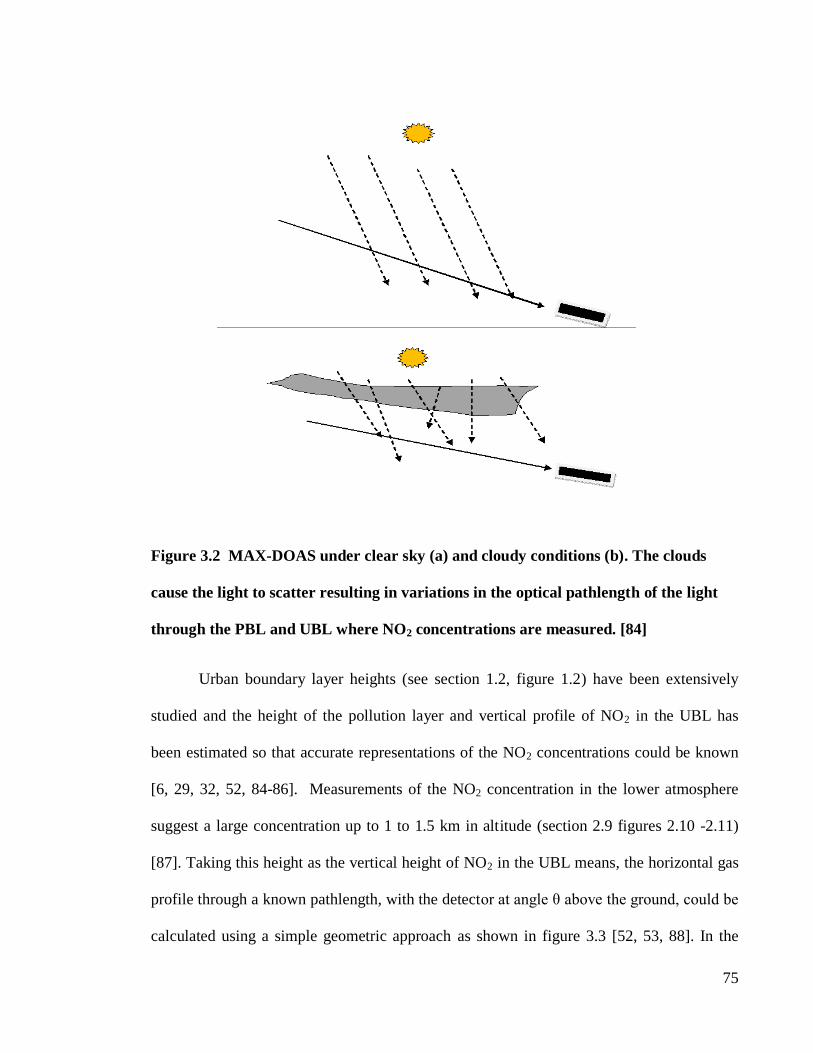
75

Figure 3.2 MAX-DOAS under clear sky (a) and cloudy conditions (b). The clouds

cause the light to scatter resulting in variations in the optical pathlength of the light

through the PBL and UBL where NO2 concentrations are measured. [84]

Urban boundary layer heights (see section 1.2, figure 1.2) have been extensively

studied and the height of the pollution layer and vertical profile of NO2 in the UBL has

been estimated so that accurate representations of the NO2 concentrations could be known

[6, 29, 32, 52, 84-86]. Measurements of the NO2 concentration in the lower atmosphere

suggest a large concentration up to 1 to 1.5 km in altitude (section 2.9 figures 2.10 -2.11)

[87]. Taking this height as the vertical height of NO2 in the UBL means, the horizontal gas

profile through a known pathlength, with the detector at angle θ above the ground, could be

calculated using a simple geometric approach as shown in figure 3.3 [52, 53, 88]. In the

76

diagram, in figure 3.3, h is the height above the ground of the observer and an approximate

value for d is calculated distance observable through the Earth’s atmosphere at that height.

Figure 3.3 Viewing geometry of the front end optics of the novel system. The

determination of d, pathlength, is found using the radius of the Earth, Re.

hRhd e22 Equation 3.3

where, h is the height of the observer and d the pathlength observed. Re is the radius of the

Earth ~ 6371 km. The angle, between Re and distance d is a right angle, so for a height of

10 m (0.01 km) from the ground, d ~ 11.29 km. The measurements made using this

approach could then be compared to established methods such as long path DOAS, UV

absorption measurements and CL and even satellite data [5, 89, 90]. Hao-yi et al [88] show

that the Differential Absorption D can be approximated if the angle between the observed

columns through the atmosphere is equal to the solar zenith angle then the value for D is:

d

Re

Re

Height (h) of

detector from the

ground h

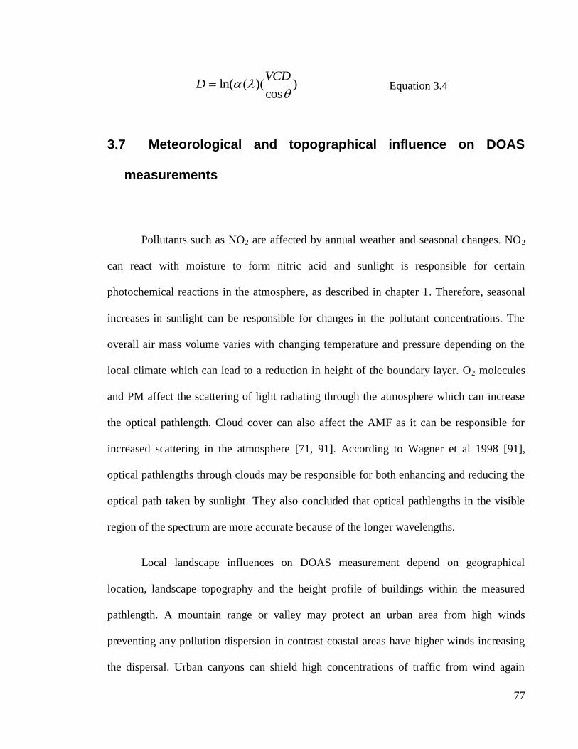
77

)cos

)((ln(

VCD

D Equation 3.4

3.7 Meteorological and topographical influence on DOAS

measurements

Pollutants such as NO2 are affected by annual weather and seasonal changes. NO2

can react with moisture to form nitric acid and sunlight is responsible for certain

photochemical reactions in the atmosphere, as described in chapter 1. Therefore, seasonal

increases in sunlight can be responsible for changes in the pollutant concentrations. The

overall air mass volume varies with changing temperature and pressure depending on the

local climate which can lead to a reduction in height of the boundary layer. O2 molecules

and PM affect the scattering of light radiating through the atmosphere which can increase

the optical pathlength. Cloud cover can also affect the AMF as it can be responsible for

increased scattering in the atmosphere [71, 91]. According to Wagner et al 1998 [91],

optical pathlengths through clouds may be responsible for both enhancing and reducing the

optical path taken by sunlight. They also concluded that optical pathlengths in the visible

region of the spectrum are more accurate because of the longer wavelengths.

Local landscape influences on DOAS measurement depend on geographical

location, landscape topography and the height profile of buildings within the measured

pathlength. A mountain range or valley may protect an urban area from high winds

preventing any pollution dispersion in contrast coastal areas have higher winds increasing

the dispersal. Urban canyons can shield high concentrations of traffic from wind again

78

reducing dispersion the high temperatures associated with urban areas can also reduce the

dispersion of pollution by wind [92].

As this project involves the development of a portable measurement system to

determine NO2 concentration in an urban environment, specifically Dublin city, a brief

description of the weather conditions expected there is now given. The city is situated along

Ireland’s east coast with the River Liffey running through its centre. There is a low

mountain range located to the south and the remaining landscape to the west and north of

the city is low lying, where agricultural activity is the main source of industry. The city is

approximately 115 km2 in area. The diurnal variation of wind speed in Ireland is

considerable. The variation is more pronounced in the summer months than in winter [93].

This is caused by the land surface heating early in the day, which increases the mixing of

the faster-moving air at higher altitude than with the air near the surface. The strong winds

are responsible for the pollutant gases like NO2, mixing in the atmosphere and the

transportation of the gases throughout the country [11]. In the average day, specifically the

late afternoon and evening, the surface heat of the land diminishes which causes the wind

speed to decrease during the night. This effect is more noticeable during the summer

months. Variation in the wind direction in Ireland is mostly westerly and southerly from the

Atlantic, but there may be northerly and easterly winds at other times of year. The average

maximum temperatures in Ireland range from only 180

Celsius in the summer to 80 in the

winter with on average less than 10 days of frost on the coastal areas. This variable weather

in Dublin and Ireland [93], with a moderate climate, show that the transport of pollution is

dominated by wind direction from the west, off the Atlantic, and with the variable

temperature there is good atmospheric mixing of gas pollutants. The weather conditions

79

and the resultant effects on pollutant mixing in the lower atmosphere justify the need for

constant monitoring of pollution concentrations.

The strong winds which cause the transportation of the pollution in urban areas (section

1.5) validate the need for a portable, inexpensive spectroscopic system to record local gas

concentrations.

3.8 Cost analysis of commercial and mini-DOAS systems

A comparison of the expense of commercial DOAS and the passive DOAS systems

shows considerable differences between the two. However the larger expense required for

commercial systems would be worthwhile if accurate measurements of a complete diurnal

variation of more than one analyte were required. Larger Commercial DOAS expense is not

just from the cost of the system itself but also from the fixed light sources or retro-reflectors

and installation of the spectrometer and the receiver/transceiver. All light sources and the

spectrometer will require mains power supply. The Xenon lamps used in DOAS typically

have a lifetime of 2000 hours and can cost up to €500. Calibration of commercial DOAS

will also require considerable expense as a specially designed calibration cell is used to

meet the dimensions of the overall system. Overall the system can range in value from a

basic package of €50,000 up to €200,000 including calibration gases and lamps[94].

In contrast, the passive DOAS miniaturised spectrometers are relatively

inexpensive and can range from €2000 to €5000 and optical fibres and lenses can be

purchased for less than a few hundred euro. Software packages for DOAS spectral analysis

can also be performed with existing software that may already be available e.g. Matlab,

80

Simulink and LabView. Alternative inexpensive light sources can possibly be employed for

nightly measurements of NO2 or other analytes. Light emitting diodes are ideal as they are

inexpensive, can be powered independently of the mains output and are relatively

inexpensive compared to other sources.

3.9 Summary

Current Active and Passive instrumentation show how DOAS can be applied to the

measurement of NO2, in particular, the various applications of Passive DOAS used to

measure both tropospheric and stratospheric NO2. Satellite data collected by NASA and the

ESA provides additional data on the vertical column density of NO2 and other analytes

which have been shown to correlate with ground based instruments. Another application of

optical absorption spectroscopy is COSPEC and the flyweight system FLYSPEC which is

similar to DOAS but has been predominantly used for volcanic measurements.

The development of the Passive novel-DOAS instrumentation requires software for

data analysis of measured spectra, which can be very sophisticated, however, using a

simplified approach to the determination of D, means that commonly available software

such as Matlab can be used. The viewing geometry of the instrument is crucial to

determination of NO2 concentration in either the stratosphere or the troposphere.

Meteorological conditions and light scattering by particles in the air can affect the

pathlength of the received light but comparative methods such as CL or Active Long Path

DOAS could provide data for correlation.

81

The passive novel-DOAS system for the measurement of NO2 in the lower

atmosphere close to the surface would provide results that would be of benefit to scientific

research and air quality monitoring. The instruments can be devised using inexpensive

hardware and commonly used software applications. Data retrieved could be compared to

existing methods to determine correlation and an estimation of the optical pathlength being

used. Cost effective light sources such as LEDs may also be utilized for night or low light

level measurements increasing the flexibility of an inexpensive instrument.

82

CHAPTER 4 Materials and methods

4.1 Introduction: Portable in-situ detection system

Typical DOAS systems described in the previous chapters are divided up between

the large setup of commercial systems and scientific DOAS apparatus designed for long

term atmospheric or volcanic research. The instrument described in this chapter was

developed from rigorous optical bench tests, laboratory tests of gas samples, light sources

and optical alignment. An algorithm shown in Appendix II, was designed using Matlab

software to analyse the spectrum of light passing through a gas sample determining the

absorption and differential absorption and tests were repeated to compare these results.

Ultimately the instrument will be unique in its ease of use and portability, thus allowing

greater flexibility for future applications and greatly reduced cost for NO2 detection.

4.1.1 Instrumentation and sample requirements

The choice of detector for DOAS applications can vary as the technique is capable

of detecting analytes across a broad wavelength range. As the work described here focuses

on the detection of nitrogen dioxide the wavelength range is determined by the NO2

absorption cross section as described in literature (Schneider [41], Vandaele [43], Burrows

[75], Bogumil [44]). There are significant absorption features for NO2 in the range 400 nm

83

to 500 nm, particularly at 435 nm and 440 nm, so a detector operating in the visible range

would be ideal. This makes it suitable for laboratory experiments as readily available

visible light sources can be used to test the samples.

The optical alignment of the detector should be adjustable to measure different parts

of the sample if necessary. This is easily achieved in the laboratory. The following are

features of the proposed system. The detector required to analyse the spectral range where

absorption is known to take place must have low power needs, portability and have a

suitable spectral range and optical resolution for the detection of NO2. One of the most

common spectrometers used in Multi-Axis-DOAS is the USB miniaturised fibre optic

spectrometers produced by Ocean Optics [95], several of which have been used in DOAS

measurements from the earlier S2000 to the later HR4000 spectrometers (Ocean Optics,

Dooly(HR2000) [96], Fitzpatrick(S2000) [97], Chen(HR4000) [98]). The work here

describes tests performed with three spectrometers specifically the USB2000, USB4000

and the Maya2000 models available from Ocean Optics. Initially, the optical alignment of

each of the spectrometers was tested with an optical fibre and collimating lens attached and

then the setup was adjusted for different samples and a field apparatus was developed.

The first samples used in the laboratory tests in this research were gas filled

polypropylene (PP) bags. Each bag was filled with air with known amounts of nitric oxide

injected. This mixes with the air to form nitrogen dioxide at predetermined concentrations.

The experimental procedure used a tungsten halogen lamp as a broadband light source

fixed with an optical fibre and a collimating lens to produce a collimated beam through the

sample. The lenses are coupled to the fibres and each sample is placed between the emitting

and receiving lenses. Figure 4.1 shows a schematic of the bench top setup for the bags and

84

the fibres which are attached to stands which can be adjusted to improve the alignment of

the light through the sample. A rail was also used to manoeuvre the setup with each bag

sample.

To improve the accuracy and precision of the novel-DOAS system, custom

designed calibration cells were eventually used as samples with known concentrations that

were a suitable size to be placed in front of the receiving optics, as shown in figure 4.1.

Initially, baseline tests were performed on the receiving optics including a determination of

the field of view (FOV) of the collimating lens when attached to an optical fibre [95]. The

alignment of the receiving setup is collimated with a beam from the emitter. The lens is

also compared to a diffuser (also known as a cosine corrector [95]) which has a field of

view of 1800. The spectral range of the lens and optical fibre, when coupled to each

spectrometer, were also examined with a broadband light source. Finally, the affect of an

adjustable aperture and collimating cylinder attached to the lens were used to control the

amount of light entering the optical system to avoid saturation and control the viewing

direction. An examination was made throughout of the spectral analysis algorithm to

confirm the absorption profile of NO2 was analysed as accurately as possible.

85

Figure 4.1 Optical fibres coupled to collimating lens aligned with each other on a

bench. The bench allows the adjustment of the emitting and receiving fibres for

alignment on either side of the polypropylene bag.

4.2 Optical instrumentation

The optical components of the detector need to be capable of detecting a large

sample volume that will provide enough information to determine the average

concentration of the analyte. For DOAS, the commercial optical system can detect the light

emitted by a xenon lamp over a path of up to 2 km or, if retro-reflectors are used, up to 10

km. The optical system of the OPSIS commercial system, as described in chapter 3, uses

mirrors of 100 mm in diameter for the emitting and receiving optics, with beam divergence

of ~4 mrad. The system developed for this research requires a smaller optical setup but will

86

still need to detect a large cross section of the light path being monitored. The area viewed

by the receiving optics is known as the FOV. For the active DOAS systems, the optics are

designed so that the FOV is compatible with the path lengths that are possible using the

artificial light sources. For the passive systems, the FOV needs to be maximised for

measurements of the layers of the atmosphere under investigation.

The laboratory measurements were designed to detect NO2 concentrations through

both PP bags and calibration cells. The light source could be fitted with an optical fibre and

lens for a clearly visible beam of light to pass through the sample or without the fibre and

lens for a broad beam illumination of the sample (seen in figure 4.1). As stated, the optical

elements will determine the alignment and focal length of the system. The receiving optics

needs to be able to detect the light with minimal adjustments and, for the laboratory

specifically, the setup needed to be stable for repeat measurements. The FOV could be

determined by using the same receiving optics attached to a source and measurements then

made of the divergence of a focussed beam through the lens and focal length. Overall, the

optics chosen must be capable of viewing the samples or atmosphere adequately and detect

light in the same wavelength range where the DOAS calculation will be performed.

The optical characteristics of the collimating lens are determined by the size and

manufacturing material, usually silica for transmission of UV and visible light, such as the

BK-7. Made from a Boro-Silicate, crown glass can be more suitable for visible

measurements. The lenses are designed with a thread to fit onto the ferrule connecting them

to Ocean Optics fibres. The focal length is determined from Equation 4.1, where f is the

focal length, typically in cm or mm, and u and v represent the object distance between the

lens and object and the image distance between the lens and a focussed image.

87

uf

11

v

1 Equation 4.1

The divergence of the beam from the lens is related to the diameter and the focal

length. The 74-UV Ocean Optics lens has a diameter of 5 mm and a focal length of 10 mm

and an estimated acceptance angle of 250. The divergence of the 74-UV is ~26.5

0 and thus

it has a half-angle divergence of 13.250.

The optical fibres use the principle of total internal reflection to transmit light from

one end of the fibre to the other. Figure 4.2 shows the transmission of light in the fibre. The

fibre is composed of the central core and the outer cladding layer. The light entering the

core of the fibre is internally reflected at a critical angle and subsequently reflected off the

cladding lining the inside of the fibre. The fibre f-number, f/#, is related to the size of the

entrance aperture where an aperture with f/# of f/2 is larger than f/4 for a narrower aperture

(equation 4.2).

Figure 4.2 Transmission of light in optical fibre occurs as the light enters at the

critical angle and subsequently reflects off the cladding as it travels to the opposite

end.

nf

nc

nc

88

The square root of the Numerical Aperture (N.A.) of an optical fibre is related its

gathering power and is calculated from Equations (4.3 , 4.4) [99].

f/# = f/Diameter Equation 4.2

Equation 4.2 is used to calculate the f/# using the focal length of a lens and the diameter of

the lens. For optical fibres the f/# equation 4.3 is used.

ANf ./# Equation 4.3

The numerical aperture can also be calculated from the refractive indices of the fibre core

and cladding (4.5). For the novel system to have an effective field of view, N.A. must be

close to the effective N.A. of the rest of the instruments optical configuration. In equation

4.4 θ represents the acceptance angle of the fibre optic, the half-angle divergence of the lens

should then be close to the same magnitude of this angle for an ideal field of view.

sin.. nAN Equation 4.4

)(.. 22

cf nnAN Equation 4.5

The numerical aperture of the fibres used in this research was 0.22 with core diameters of

600 µm. The acceptance angle of the fibre is then ~ 120 almost equal that of the half-angle

divergence of the lens.

89

4.3 Optical alignment

The optical throughput of the overall receiving system consists of the collimated

light from a transmitting optical setup entering the lens of the receiving optics. For the

system being described here, the entrance optics consists of a collimating lens connected to

a fibre by standard Ocean Optics SMA905 connector. The light propagates through the

fibre and into the spectrometer, as shown in figure 4.3, the shaded area indicated by the box

and red lines represents the optical fibre ferrule and frame of the lens. The combination of

the entrance slit of the spectrometer, the mirrors, which direct the light onto a grating and

towards the CCD detector, the size and alignment of the grating and size of the detector

determine the amount of light exposed to the detector elements. The complete optical

arrangement of the entrance optics determines the signal developed measured by the

spectrometer. The relationship of each optical element in the whole optical system can be

determined as the product of all the optical components from the size of the entrance

aperture to the area of the CCD detector inside the spectrometer.

90

Figure 4.3 Schematic of how light rays passing through a sample are collimated by

lenses and optical fibres.

As discussed in chapter 2, modern DOAS measurement devices use a variety of

detectors, from the PMT of the larger commercial systems to the photodiode array and

charge coupled devices of smaller detectors. PMTs detect light which is converted to an

electrical signal by the photoelectric effect. They are able to detect very low light levels,

which are directed at several electrodes increasing the signal, making them ideal for the

detection of the xenon lamp source over the long light paths used in active DOAS systems.

Photodiode arrays are, as the name suggests, arrays of light sensitive semiconductor devices

used for the detection of specific light wavelengths or a range of wavelengths. These can be

designed to detect specific wavelengths associated with a chosen analyte.

Collimating

lenses

Sample

Optical fibre and

attached ferrule

(shaded)

Collimated

rays

91

4.4 Miniaturised spectrometers and charge coupled devices

The typical miniaturised spectrometer used in modern DOAS applications is the

type manufactured by Ocean Optics and Acton. The Ocean Optics spectrometers use a

Czerny-Turner design, see figure 4.3.

Figure 4.4 Czerny Turner spectrometer design. The light enters at the aperture where

the optical fibre is coupled to the spectrometer. The light reflects off the opposite

mirror onto the diffraction grating, the diffracted light is then collimated by the

second mirror and reflected onto the CCD detector.

The main components of this design are shown in figure 4.3. They include the

entrance slit, diffraction grating and charge coupled device (CCD) detector. The entrance

slit is chosen for the best optical resolution for the spectrometer that is used. The diffraction

grating will have a chosen spectral range depending on the material and blaze angle and the

Entrance slit

Mirrors

Diffraction Grating

Charge coupled

device (CCD)

detector

92

dispersion, lines/nm, is determined from this range divided by the number of detector

elements. The optical resolution is the product of the dispersion and the pixel. For example,

the resolution of a USB4000 with 3648 detector elements and a slit width of 25 microns

and optical resolution of ~1.34 nm will have a pixel resolution of ~7.5 pixels. Alternatively,

the USB2000 spectrometer has 2048 detector elements and is also a front illuminated

spectrometer; the differences between front illuminated and back illuminated spectrometers

are outlined in detail in this section and section 4.5. The resolution provides more detail in

each recorded spectrum making it possible to identify the attenuated features of each

spectrum which is caused by gas absorption. But the USB4000’s greater resolution allows

for a greater accuracy in the determination of differential absorption (D) as the absorption

and attenuated features are more readily identifiable.

Diffraction gratings can be either transmission gratings or reflection gratings.

Transmission gratings consist of slits for light to pass through or a transparent material with

grooves etched into one side. The reflection gratings have ruled grooves into the reflecting

surface. The density of these grooves determines the dispersion and therefore the spectral

resolution. Modern diffraction gratings for spectroscopy use reflection gratings with blazed

[99] rulings that have sharp edges to reduce the amount of light wasted in their operation,

making them ideal for applications like the one described in this research.

The ideal detector used in the miniaturised optical fibre detector is the Charge

Coupled Device semiconductor detector. Charge coupled devices (CCDs) are sensor

devices developed by GE Smith and WS Boyle for Bell laboratories in the 1970s.

Originally designed for image sensing, they have numerous applications including

commercial applications like memory and cameras. The principle of operation behind the

93

charge coupled device involves light illuminating the surface of a solid state material (e.g. a

metal oxide) and then the excited charge is transferred through the semiconductor in a

discrete form to an adjacent area where the charge is stored [100]. The metal oxide layer is

known as a potential well which forms when the electronic charge is applied to the device.

CCDs in miniaturised spectrometers can have a lens close to the surface of the detector to

maximise the light sensing of the detector.

Figure 4.5 Structure of charge coupled device with three electrodes, a potential well is

formed under each electrode where the electronic charge is built up before conversion

into an electronic signal.

The potential wells transfer the accumulated charge through the

semiconductor layer. As indicated in figure 4.4, the potential well is formed beneath the

middle electrode when a positive voltage is applied while the others electrodes have a zero

applied voltage. The difference in the electrodes creates a potential barrier confining any

charge carrying electrons. By adjusting the potential in sequence, the charge is sequentially

Sem

iconduct

or

e.g.

Si

Gate Electrodes

Metal O

xid

e

94

transferred through the semiconductor material to the output. The 3 electrodes (figure 4.4)

form a pixel which can be grouped in sets and when a series of these pixels are formed they

create what is known as a vertical and horizontal register. The CCD is operating as a charge

transfer device throughout this process. The vertical register consists of a photosensitive

column, e.g. 64-128 or more pixels that transfer the charge to the horizontal register. The

charge is then transported to an amplifier and converted to a voltage see figure 4.5.

Although there are a few different ways that the transfer process is used, the most

common for spectroscopy is the Full Frame Transfer (FFT) process. Frame transfer in

CCDs uses two vertical shift registers, a photosensitive and a storage section as well as the

horizontal register and the output section. Once the charge builds up in the potential well, it

is transferred to the vertical photosensitive section which converts light into electronic

charge. The frame transfer is processed in this vertical register, and then transferred to the

horizontal register and from there to the output. All parts of the device except for the

photosensitive section are protected from light by an opaque material. FFT CCDs are

designed without the storage area so the collected light is transferred directly from the

photosensitive section to the horizontal register as shown in figure 4.5.

95

Figure 4.6 Full frame transfer process of a CCD detector. The electronic signal builds

up in the vertical shift register and passed to the active area. From here it is

transmitted to the horizontal register followed by the amplifier.

4.5 The back illuminated charge coupled device

The structure of CCDs can also vary according to how the light passes through the

semiconductor. Back illuminated CCDs (BI-CCD) for spectroscopy e.g. Maya2000 are

ideal for low light levels and are responsive in the UV region of the spectrum. The principle

of operation compared to the front illuminated CCD (FI-CCD) is, as the name suggests, the

illumination of the back of the CCD array. This means the light enters the detector through

the silicon before reaching the electrodes. No light is lost by reflection or absorption as in

Horizontal Register

Ver

tica

l S

hif

t R

egis

ter A

ctive A

rea

Amplifier

96

the FI-CCD, so the BI-CCD has a much higher quantum efficiency [101]. BI-CCD

detectors are usually thinned to reduce the distance the light travels. However, the layers of

Silicon the light passes through create optical cavities that result in Fabry-Perot etalon

features in the viewed spectrum especially in the near-IR [102]. The structural differences

are shown in figure 4.6. The etaloning is in spectral and the spatial features.

Figure 4.7 A Back illuminated charge coupled device. Note thinned silicon layer where

the spectral etaloning is known to occur.

The spectral etaloning causes the intensity to vary in magnitude with wavelength.

This occurs because when the light reaches the poly-silicon electrode layer there is a

change in refractive index, reflecting light back into the CCD. For some wavelengths the

light will be reflected back several times. This effect enhances the quantum efficiency of

the CCD because more light is turned into signal but it reduces the amplitude of the signal

due to absorption and reflection. In spatial etaloning there is also a variation in intensity

amplitude with the thickness of the CCD especially if the thickness of the silicon is not

consistent.

As well as spectral and spatial etaloning, there can be spectroscopic etaloning where

the wavelength of the light changes across the BI-CCD. Most of these effects in BI-CCDs

97

occur in the longer wavelengths of the near infra-red region. Spectroscopic binning can

counter these effects where the vertical and horizontal shift registers sum their pixels before

moving to the next stage. This action along the two columns will average out the

interference patterns created by the features in the Near IR. Anti-reflective coatings can

also be used to optimize these longer wavelengths. The vertical line binning operation can

also reduce the signal readout time. The disadvantages of the etaloning in the recorded

spectrum of the Maya2000 are illustrated in the results chapter 6. Ultimately, of the three

spectrometers, the USB4000 was chosen because of its optical characteristics and how well

the absorption spectrum of NO2 compares to NO2 spectra from the literature.

4.6 Dark current and noise

The types of noise encountered when using CCD spectrometers are caused by both

electronic and physical effects. The dark current is the observable signal present when no

light is being received by the spectrometer. It is a thermal effect occurring in the different

regions of the CCD. Within the dark current, both the signal received with no light and the

noise in the system is present. This noise in the signal is dependent on the integration times

being used which can be reduced by varying the integration time without losing any

information when taking measurements. To reduce the effects of thermal noise, it is

important that the spectrometer CCD should not be allowed to overheat. This can be

difficult for long term measurements but there are several ways to counter this, such as

cooling with a combined Peltier element and heat sink or with a D.C. fan. If the sunlight

being acquired for atmospheric measurements is changing quickly, and/or if the wind speed

98

is high and cloud cover is rapidly changing, then low integration times are needed. The

signal-noise ratio, S/N, of the detector is the total signal divided by the noise. The number

of scans made by the detector can be used to improve the S/N, which increases as 1/√n,

where n is the sum of spectra added [101, 103].

Readout noise is a type of noise created in the output stage of the CCD. The metal

oxide semiconductor field effect transistor (MOSFET) amplifiers produce an electrical

noise that determines the lower limit of detection of the detector. The Dynamic Range, DR,

of a CCD detector is dependent on readout noise by equation 4.5.

Dynamic Range = full well capacity/readout noise Equation 4.5

Other forms of noise affecting the system operation include:

Fixed pattern noise caused by the variation in the response of neighbouring pixels.

Shot noise affected by the statistical changes in the number of photons incident on

the detector.

Dark Shot noise when the dark current is affected by shot noise. Reducing the dark

current will lower the effects of dark shot noise.

The overall noise of the system can be reduced by keeping the detector at a low temperature

and using an integration time that yields information about the analyte but is not heavily

laden with noise effects. Typical noise and dynamic ranges for the miniaturised

spectrometers used in this work are described in table 4.1 below.

99

Parameter USB2000 USB4000 Maya2000

CCD Model Front Illuminated-

CCD

Front Illuminated-

CCD

Back Illuminated-

CCD

No. of pixels 2048 3648 2048 x 14

Readout (dark) noise 2.5 50 13

S/N ratio 250:1 300:1 350:1

Quantum Efficiency % ~40-50 ~40-50 ~90

Spectral Range 650nm 650nm ~935nm

Dispersion nm/pixel 0.32 0.18 0.45

Table 4.1 Characteristics of the three miniaturised spectrometers used in the

development of the novel DOAS device

4.7 Power and software requirements

The basic power requirements for a portable DOAS system will come from the

supply of the computer used to record and control the spectrometer measurements.

Miniaturised spectrometers like the Ocean Optics models use low power from 250mA to

500mA at 5 Volts with a D.C. supply. The system described here uses a laptop connected to

the spectrometer by USB cable which powers the spectrometers. The laptop can operate on

its own in-built battery or from a mains supply when recharging. The battery lifetime for

any laptop can vary and may decrease over time, but if operating well can last up to 7 hours

in newer models. As the software needed to run the spectrometer can be added easily to the

laptop operating system, any laptop can be used. So for long term measurements, when a

mains power supply is not readily available, more than one laptop could be used.

The requirements for the software used to collect spectra for DOAS analysis are that

it should be capable of representing the data as raw intensity, absorption and it should be

100

possible to save the data in a common format e.g. text files. The primary software used with

Ocean Optics spectrometers is SpectraSuite. This software allows the user to control the

integration time and the number of scans for each. SpectraSuite also allows the user to save

the data in several ways including text files and can present the data in raw intensity,

transmission, irradiance and absorption. Figure 4.8 shows a screen shot of typical data of

gas samples measured using the USB4000 spectrometer [95], the data is presented in

intensity versus wavelength in a) and absorption versus wavelength in b). The units for the

intensity and absorption spectra are a digital number on the y-axis and wavelength in

nanometres for the x-axis the wavelength range shown is between 300 nm and 700nm.

a)

101

b)

Figure 4.8 Raw intensity spectrum (a) of a tungsten light source used in the laboratory

as a reference measurement Io and an absorption spectrum (b) for NO2 with

wavelength on the x-axes is between 300 nm and 700 nm.

The absorption spectrum shown in 4.7 (b) is calculated for NO2 using a visible light source

with a peak wavelength between 500 nm and 600 nm. The spectrum of the lamp in 4.7 (a)

is low between 400 nm and 300nm. The effect of this low signal produces a noisy signal in

the absorption spectrum, 4.7 (b) in this range. However, the NO2 features are identifiable

between 400 nm and 600 nm with significant peaks between 435 nm and 500 nm.

For measurements over several days, the software allows the user to control

measurements taken for designated times which are saved in one folder. Dark subtraction

can be done either with SpectraSuite or during the data analysis with Matlab or other

102

software. A dark current file should be saved often for continuous analysis. Other

SpectraSuite functions include stray light correction and spectra overlay for comparing

different results. Data can also be reformatted if necessary using the SpectraSuite menu to

convert files to text etc.

4.8 Final setup for laboratory and field measurements

In chapter 6 the results of measurements taken with the miniaturised spectrometers

used for this research are described. The results will show that the USB4000 was chosen for

the final setup of the novel-DOAS because of the accuracy of the results with the

calibration cells.

The experimental setup used to test the spectrometers for this research consisted of

adjustable stands attached to an optical bench (see figure 4.1). For tests of path changes

between the source and detector, a metre long rail was used. The stands are attached to

either the bench or rail and adjusted to improve the optical alignment and counter any

saturation of the signal or refraction by the sample material and NO2 gas. The primary light

source used in the laboratory is a tungsten lamp with a broad profile and initial tests were

done with the USB2000 spectrometer.

4.8.1 Sample preparation and measurements

The procedure is developed with PP bag samples that are filled with air and small

amounts of NO added to create a concentration of NO2 that will be used to determine if the

detector can identify the characteristic profile of the gas in air. Several tests are performed

103

with the bags and the USB2000 to develop a comparison of absorption (A) and differential

absorption (D). To improve the accuracy of the measurements, the USB4000 and

Maya2000 are later used. Ultimately, the USB4000 spectrometer was chosen because of

improved resolution. The signal to noise ratio and the results of tests performed on the

calibration cells are described in more detail in chapter 6.

For the PP bags, the pathlengths are taken to be the width of the sample. The bag

widths are between 18cm and 20cm, approximately the thickness when the bag is fully

inflated. Preparation of the NO2 bag samples involved pumping air into the bags until they

are half full then injecting millilitres of NO into each bag which would then be filled with

more air. Usually three samples are prepared and a bag filled solely with air is used as a

reference sample.

Eventually, the calibration cells took the place of the bags because of the accurate

concentrations and the suitable size compared to the optical setup. The final optical setup

consisted of a spectrometer with a 1 metre or 2 metre optical fibre, collimating lens,

collimating tube and adjustable aperture. The whole apparatus was fitted to a camera stand

with a rotational platform for measurements of various azimuthal and elevation angles.

4.8.2 Optical bench measurement procedures

The procedure for testing each sample involved placing the reference sample (air

sample) into the path of the detector with the light from the source directed at the receiving

optics. The integration time and sampling average are chosen and the appropriate settings

104

made. A dark current measurement is recorded while the lens is covered this will later be

subtracted from each recorded intensity spectrum. The raw intensity spectra are then

recorded as a reference spectrum and saved. The reference sample is then removed and the

NO2 samples are placed in the path. A spectrum is recorded for each and then the procedure

was repeated 5-10 times. For measurements of A, an absorption spectrum is recorded after

each NO2 sample is measured. Once the data was collected it is examined in a Matlab file

which used a purpose built algorithm to determine the dark subtraction, mean and standard

deviation, D and A for each sample. More than one dark spectrum is taken for all

measurements, as the dark current could vary while the spectrometer is in use. Figure 4.8

shows a bag filled with air placed in the optical bench apparatus. The concentration of NO2

in the bags is calculated with a known path length and α’ which is determined from the

literature and this concentration could be compared to the expected concentration value.

Figure 4.9 Polypropylene bag placed in the path of a collimated light beam produced

by a tungsten source, optical fibres and collimating lenses, detected by a USB4000

detector.

105

The bags are also tested for their stability over time with absorption measured over

periods of time of a few minutes after preparation, hourly and once a day for one week.

These tests are used to determine if the actual concentration is above or below the expected

results and by how much the concentration changes for periods of time. It is expected that

the concentration immediately after mixing would be low for a half hour. When the NO is

converted to NO2, the concentration should have some stability for a minimum of a couple

of hours until the gas chemically reacts with light or begins to form a deposition layer on

the bag itself. The rate of reaction for each bag is monitored with particular attention to

low concentrations in case they drop below the limits of detection before accurate

examination of the sample could be performed. Once filled, different paths through each

bag are tested to compare if each pathlength had the same concentration this would confirm

that the concentration is uniform throughout the bag.

Initial tests of the bags show large differences between the expected concentrations

and the measured results. Tests were conducted on diluted bags with a CL instrument to

determine if the results which required lower concentrations were independent of the

instrument and a result of the bag material (polypropylene) or the filling procedure.

4.8.3 Calibration

The calibration cells were chosen as an alternative to the PP bags because of the

stability of the cells and their use for similar methods like COSPEC [79] described in

chapter 3. The calibration cells were manufactured by Resonance Ltd [104]. Each cell has a

quartz body with a short stem, a diameter of 22 mm and a thickness of 14.5 mm. The cells

106

are ideal for testing with the new system (section 6.4) because the size of each cell means it

is possible for placement in front of the system optics in a way that is not as cumbersome as

the PP bags. Four cells were purchased with concentrations equivalent to typical

atmospheric concentrations for NO2. Table 2 shows the differences in concentration for 1

metre and 10 km for each cell. Tests performed with the calibration cells include accurate

determination of each cell NO2 concentration and tests of the NO2 concentration stability

over time with exposure to a light source. The cells are expected to have a stable

concentration of up to two years, according to the manufacturer. The absorption of light in

the 430nm – 445nm range is measured and recorded and the mean and standard deviation

was determined. In chapter 6 it is shown that the known concentration of the cells allowed

for an assessment of the three miniaturised spectrometers and showed that the USB4000

spectrometer (section 6.6) yielded the most accurate results, justifying its use in the field

measurements described in chapter 6, section 6.9.

Cell concentration.

Equivalent for 1m path length 10km path length Concentration error %

1 Atmospheric air 0 ppb 0

2 5ppm-m 0.5ppb ±10

3 20ppm-m 2ppb ±10

4 50ppm-m 5ppb ±10

Table 4.2 Concentrations of calibration cells for 1m in the laboratory (in ppm) and a

10km pathlength (in ppb) equivalent to those that can be measured in the atmosphere

107

The mean values of A(λ) for each cell are compared to the mean values for D(λ)

with standard deviation for 10 measurements of each cell. The cells, shown in figure 4.9,

have a fixed concentration so the spectrum of α could be determined with a fixed path

length. The differential α(λ)’ can be found from significant features in the wavelength

range mentioned above. This coefficient α(λ)’ would be more instrument specific than the

values taken from the literature. For example, the instrument resolution between the results

of Solomon [52], which were taken in 1987, would be very different to those of Bogumil

(2003) [44] and the USB4000, but α(λ)’ should still be within a small margin of error of the

literature values.

Figure 4.10 Gas calibration cells. Each cell is 1.4 cm thick and each one is fitted with a

stem for placement in front of the detectors lens.

The cells are also tested for changes in light intensity using neutral density filters

(NDF). It was expected that D(λ) would be independent of the light intensity except at very

low light levels close to the limit of detection (LOD) where the signal to noise is low.

108

4.8.4 Urban measurement of NO2 with the novel-DOAS

To test the effectiveness of the novel instrument for measurements of the urban

atmosphere, several tests were developed to determine the instruments ability to profile the

UBL NO2 variation and the vertical variation (see sections 6.8 and 6.9). These

measurements are also used to determine the differences between clear and cloudy days and

for comparisons with existing methods to determine the approximate LOD of the

USB4000. The spectra of sunlight are examined in detail to identify the ideal

wavelengths for analysis, specifically, wavelengths where there was minimal interference

from Fraunhofer lines and therefore the Ring effect [37]. The chosen range would also have

low interferences from other species and still be a significant feature for the identification

of NO2 and determination of its wavelength. For the determination of D(λ), equation 2.14,

the feature at 439 nm – 441 nm was chosen, as it had only small interference from

Fraunhofer features unlike the feature at 435 nm.

Measurement of NO2 in the atmosphere above Dublin city required a clear view of a

path above the city. For measurements conducted over several days, only one elevation

angle is needed so the main requirements included an unblocked view of a large area of the

city preferably with an EPA-CL [24] monitor within the path. The benefits of the CL

monitor will be explained in more detail in the next chapter. The main objective of

measurements using solar light is to determine a profile of the diurnal variation of NO2 in

the atmosphere and compare the results to similar measurements in the literature, available

commercial DOAS systems as well as CL data. The measurements are expected to show

that the gas concentration will vary throughout the day with high concentrations occurring

109

at sunrise and sunset due to rush hour traffic and the photochemical reactions of NOx gases

with ozone when the Sun is at its highest solar zenith angles.

To measure concentrations that are comparable to the EPA standard requirements

for NO2, most of the measurements are setup for low elevation angles. The path length is

approximated from typical viewing geometries found from the literature and by making

comparable measurements with the CL data made available by the EPA. The USB4000

was set to measure automatically for several days with frequent dark currents recorded. In

the analysis, the dark current is subtracted and the readings recorded at low light levels and

during the night are ignored. Measurements are recorded every 10 to 15 minutes, the data

then can be presented as the half-hourly or hourly change throughout daylight hours. The

daily mean can also be determined from the data analysis.

For measurements of more than one elevation angle, the ideal locations are roof tops

of city buildings. For this research DIT buildings are the primary locations [105].

Measurements of the different elevation angles should provide data on the vertical profile

of NO in the atmosphere from the troposphere to the lower stratosphere. The integration

time of the USB4000 was set at 10ms for 100 to 500 scans averaging over 1 second to 5

seconds. The measurement of each elevation was conducted in a way to reduce the amount

of time between each measurement, as the NO2 concentration will vary with wind velocity

and the light scattering in the atmosphere can affect the length of the path length. An

adjustable rotation stage was attached to the field apparatus to ensure that the

measurements of each angle can be controlled. The rotation stage is graded with 3600

angles with 900 aligned to the zenith position. Figure 4.11 shows the front-end optics of the

field apparatus. For azimuthal angles the stand is adjusted so that the stage can show the

110

azimuthal changes. Where more than one azimuthal angle is needed, a clear view of

multiple paths is ideal. Measurements of the different azimuthal directions can be

conducted to compare any changes in concentration in different areas of the city at any one

time. These measurements were all taken at the lowest elevation angles. A more detailed

examination of elevation and azimuth can be done with multiple spectrometers

simultaneously.

Figure 4.11 Schematic of the field apparatus of the novel-DOAS with the collimating

tube and adjustable aperture fixed to the collimating lens and fibre

The calibration cells were placed in front of the USB4000 to see the effect made

when a known concentration is placed in the path, the air sample is used as a reference for

any additional effects caused by the quartz cell. If the increase in the value of D, for the

known attenuation feature where NO2 is known to absorb sunlight, corresponds to the

111

increase in concentration of each cell, then it can be assumed that the system is capable of

detecting increases in NO2 using ambient sunlight. If there is a noticeable effect when the

smallest concentration is placed in the path then the LOD of the system can be determined

and a calibration procedure developed.

Several measurements were taken comparing the light being received by the

USB4000 under different meteorological conditions. Direct measurements are taken to

compare direct sunlight spectra with the measurements of indirect light and a value of D

was calculated from each.

Different geographical locations were compared, but these cannot be done

simultaneously because of the distances involved, the number of instruments and the

meteorological conditions. Landscape comparisons can be performed with the USB4000

directed at nearby mountains and towards the sea and at urban areas to determine if any

notable changes in D could be detected.

4.9 Summary

As described in chapter 3, modern miniaturised spectrometers can be used to record

spectra with enough detail to accurately make a determination of the D at specific

wavelengths. A system consisting of a USB spectrometer with a lens, optical fibre and

collimating cylinder attached to a portable stand is ideal for measurements of different

locations without difficult installation at each location. Power usage can be kept to a

minimum and more than one system can be used to monitor a larger area if necessary. To

determine the LOD of the instrument laboratory tests were performed, tests were conducted

112

to explore the possibility of determining the correlation between absorption measurements

and differential absorption. To perform the laboratory experiments, a broad band tungsten

light sources are used to simulate the broad solar spectrum. Samples of NO2 prepared in PP

bags are used but for more accuracy quartz calibration cells are more ideal. The individual

features in a specific spectral range are where light is attenuated by the gas these are used to

determine the differential absorption and the absorption.

Atmospheric NO2 measurements are done with the novel setup. A survey of

different azimuthal directions and elevation angles are also performed. The vertical profile

of the lower atmosphere can be determined if the O3 and aerosol profile are known however

the possibility of making an estimate of the profile using the cheaper portable system is

examined. Data was collected during daylight hours for several weeks and compared to

other methods mainly CL. s

Chapter 5 will describe in further detail the comparison and correlation between

Passive DOAS and CL measurements. Along with a summary of the literature on DOAS

and CL comparisons, a description is given of the tests performed using the portable novel-

DOAS instrument and what the results of these tests were expected to reveal.

113

CHAPTER 5 Comparison of chemiluminescence and DOAS for

monitoring of NO2

5.1 Introduction

In order to calibrate the novel-DOAS system, it was first required that CL and

DOAS can be demonstrated to produce correlated results. The following chapter explores

the distribution of the monitoring stations employed by the EPA in Ireland and how CL is

used throughout Dublin city to monitor the concentration of NO2. Initially the results of CL

data and an old DOAS instrument used by DIT (section 5.3) are compared, and

comparisons in DOAS literature where both methods were used to make concurrent

measurements are reviewed. As described in chapters 2 and 3 of this thesis, determination

of the pathlength, L through which the scattered light travels can be the source of

substantial error in the calculation of the NO2 concentration using DOAS. In chapter 3,

section 3.6, the pathlength, assuming the detector is ~10 m off the ground is approximately

10 km. With this value, the concentration of a pollutant in the local atmosphere can be

estimated from the calculated values for differential absorption, D. However, the effects of

scattering light, described in chapters 2 and 3 illustrate how difficult it is to rely on fixed

values for the pathlength. Therefore, a comparison of the novel-DOAS system with a

known accurate method like CL will improve the estimates for L and the effectiveness of

the novel system to measure the concentration of NO2 in the atmosphere.

114

A detailed description of the CL instrumentation and its operation is given and of

how the results of a CL device, used by the EPA in Dublin, were compared to the novel -

OAS system being developed for this research.

5.2 Summary of literature for DOAS and CL comparisons

A comparison of UV absorption, CL and a multi-path DOAS system was made by

Williams et al (2006) in three locations in the U.S.A., Nashville Tennessee, Houston Texas

and the north east coast of the U.S., the gulf of Maine [89]. The study describes

measurements made to assess the correlation of the UV absorption data to the other

methods. The results showed that there was a good correlation between the UV system and

the CL system with some discrepancies at night and early in the morning. However,

comparisons of the Multi-path DOAS and the UV system showed very good correlation

with a variation of ±7%.The data was compared for the period between 10am and 6pm in

the evening.

Good correlations between CL and DOAS were also observed by Leigh et al.

(2006)[106]. An in-situ CL system was compared to a concurrent-multi-axis DOAS

(CMAX-DOAS) set up in Leicester (UK). The CMAX-DOAS measurements appear to be

recorded between 5am and 9pm and the weekly variations, including lower concentrations

on Sundays, are shared by the CL results.

More recent comparisons made by Chan et al. (2011) [49], Dunlea et al. [107]

comparing Tunable IR Laser Diode Absorption Spectroscopy (TDLAS) to DOAS and CL.

115

Other comparisons include those conducted by Vlemmix et al. [108], which were done with

the regional Lotos-Euros air-quality model in the Netherlands.

5.3 Dublin Institute of Technology DOAS monitor

Research has been conducted by the Dublin Institute of Technology (DIT), which

had an operating OPSIS-DOAS system with the receiver located on the roof of the Kevin

Street building as well as several emitters located in different locations around Dublin city

[5, 105, 109, 110]. Figure 5.1 shows the locations of the receiver and the 5 paths between

the receivers and the emitters.

The emitters where fixed in position on the roofs of current and former DIT

buildings and local government buildings. Due to the increased construction around the city

in the last two decades and change in ownership and use of these buildings, not all the

emitters were available for use in this project.

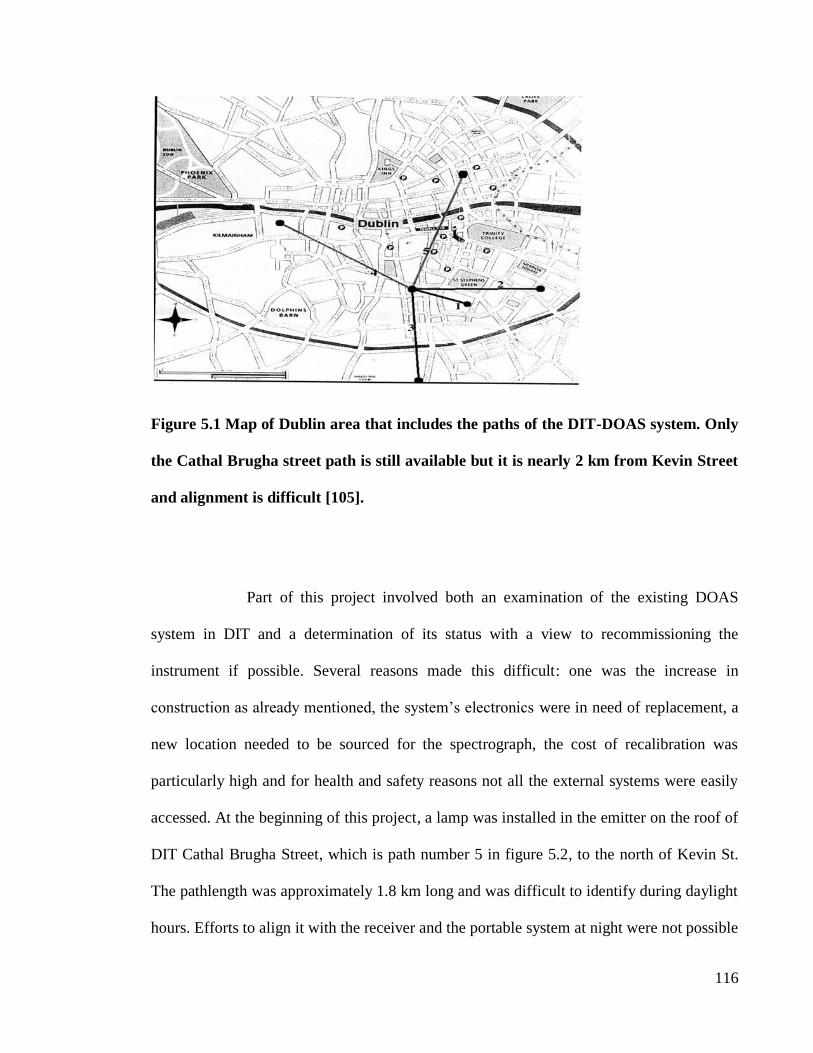
116

Figure 5.1 Map of Dublin area that includes the paths of the DIT-DOAS system. Only

the Cathal Brugha street path is still available but it is nearly 2 km from Kevin Street

and alignment is difficult [105].

Part of this project involved both an examination of the existing DOAS

system in DIT and a determination of its status with a view to recommissioning the

instrument if possible. Several reasons made this difficult: one was the increase in

construction as already mentioned, the system’s electronics were in need of replacement, a

new location needed to be sourced for the spectrograph, the cost of recalibration was

particularly high and for health and safety reasons not all the external systems were easily

accessed. At the beginning of this project, a lamp was installed in the emitter on the roof of

DIT Cathal Brugha Street, which is path number 5 in figure 5.2, to the north of Kevin St.

The pathlength was approximately 1.8 km long and was difficult to identify during daylight

hours. Efforts to align it with the receiver and the portable system at night were not possible

117

as the low power of the 150W lamp over that distance made it too difficult to detect.

According to OPSIS, any calibration of the OPSIS system is best done with a pathlength of

300 m to 1 km. It was also determined that the software of the system needed to be

extensively updated and the spectrometer would most likely require replacement

components[28].

Older data saved electronically on the DIT DOAS system did show correlation

between DOAS concentrations and Dublin based EPA CL devices, however, as shown in

figure 5.4. The graph shows how the diurnal variation of the results taken by the EPA

showed a very similar trend to the results of the DOAS. The DOAS concentrations appear

higher overall, which may be due to the DOAS results representing measurements of the

average concentration over a distance of 600 m to 1 km. It was decided that a comparison

of the portable system and the local EPA data could be used to determine the accuracy of

the new device for measurements of the local atmosphere.

118

Figure 5.2 Comparison of the data obtained from DIT-DOAS and EPA-CL

instruments for 03-05-2001

Figure 5.3 shows the CL data presented by the EPA for the Rathmines site on

Wynnefield Road. The data shows the variation in concentration for 6 days in October 2012

for O3, SO2 and NO2. It is worth noting the lower SO2 concentration in comparison to the

other two gases and how the NO2 and O3 levels vary with an apparent inverse relationship,

most likely due to the photochemical reactions described in chapter 1. The few days

presented in figure 5.3 are for the October bank holiday weekend. The data shows the day

and night variation of all three of the gases, with the daily variation appearing between the

dates marked on the horizontal x-axis. There is some reduction in the NO2 concentration

during the daylight hours and much higher concentrations during early morning and

evening. The low concentration on Sunday the 28/10/12 is due to lower traffic congestion

and the increased photolysis of the NO2 gas. It can be compared to the higher

concentrations on the Friday 26/10/12 where the NO2 reaches 50 µgm3. This is most likely

119

driven by the typical traffic congestion at the end of a working week at the beginning of the

bank holiday.

Figure 5.3 Real-time data from the Rathmines monitoring station (25th

to 3rd

of

October 2012). The NO (green) O (blue) and SO (red) data are available from the

EPA website [17]

5.4 Chemiluminescence instrumentation

As previously stated in chapter 1, the European Union regulations advise [9] that the

standard method for the monitoring of NO2 can be done by CL. CL [10] is a point sampling

technique which takes a sample of the atmosphere through an intake tube and then the

concentration of NOx, NO and NO2 are determined using a molybdenum catalytic converter

and PMT detector. Figure 5.4 illustrates the process the NOx gas takes inside the CL

120

instrument. Alternatively the DOAS method of measuring pollution is a remote sensing

method that can be setup to measure many pollution concentrations over long paths in a

typical urban environment. The two methods are worth comparing (section 5.5) as they

each have their advantages and disadvantages and have previously been shown to

complement each other [49, 89, 106, 107].

Figure 5.4 CL monitor operation. Air is sampled at the inlet and the PMT measures

light through NO or NOx gases. NO2 is then found by subtraction.

The process of CL occurs when the samples are extracted from the atmosphere in a

gas phase. In this state, they undergo chemical reactions that emit light. The reactants

transfer energy during the reaction and undergo electronic transition up to higher energy

121

levels. When the excited electrons return to lower states they release energy in the form of

photons.

The CL monitoring instrument operates by sampling the local atmosphere through a

narrow inlet tube. The nitric oxide (NO) in the air sample reacts in a cell with ozone

produced by the instrument (Reaction 5.1). The following reactions describe the order that

the NO and O3 gases are introduced to each other (Reaction 5.1 – 5.3) and their products as

well as the reaction of NO2 with the molybdenum (Mo) converter.

2

*

23 ONOONO (Reaction 5.1)

hNONO 2

*

2 (Reaction 5.2)

32 33 OMNOMNO oo (Reaction 5.3)

Single molecules of NO2 and oxygen are produced, with the NO2* molecule

retaining excess energy that is emitted as infra-red light (Reaction 5.2). The light emitted is

in the wavelength range 600 nm to 3000 nm with a maximum (IR) peak at 1200 nm and is

detected by the PMT. The sample is then directed through the Mo converter at a

temperature of 315 0C (Reaction 5.3), which chemically separates more NO from the

sample. This is then passed through the same reaction cell and the emitted light is measured

again by the PMT, see figure 5.6. This second measurement represents the amount of NOx

gas in the sample as the amount of photons released should be directly proportional to the

NO concentration. Finally, the NO2 concentration is determined by subtracting the NO

concentration from the NOx concentration [10, 24, 27].

122

5.5 Comparison of in-situ DOAS and CL

As has already been shown, there is good correlation between DOAS and CL,

(figure 5.4, and results described in the DOAS literature). Because of this and the lack of

availability of a local DOAS system, comparisons were made of CL and the novel optical

system to determine NO2 concentrations and the optical system’s LOD. For this research,

some comparison was made between the results obtained by the novel DOAS system and a

CL instrument used for another research project conducted by Trinity College Dublin.

Extensive comparisons were also made between the DOAS system and the EPA monitoring

station in Rathmines, an area in South Dublin.

The CL monitor was a Teledyne API 200A chemiluminescence analyser[24]. These

systems are designed to monitor nitric oxide, NO2 and NO concentrations. The API 200A

monitor is 18 cm by 43 cm by 60 cm in size with inlet tubing and external vacuum pump

connections. It is powered by a mains supply or a portable generator. The API 200A

instrument has a range from 50 ppb to 20,000 ppb (20ppm), and a inlet tube flow rate of

500cm3/min so approximately half a litre is extracted from the atmosphere each minute and

it has an operating temperature of 5 to 40 0C. Its central processor has several functions that

allow the operator some selectivity this is possible with the ‘multi-tasking software’.

Calibration was performed with a standard gas of known concentration held in an external

cylinder.

123

Overall, the CL systems are reliable and accurate but they are a fixed system

requiring mains access and protection against the weather and theft. CL is very accurate

and is comparable to other measurements made by CL within Ireland and the rest of the

EU. It is less susceptible to interference by other trace gas species as the measurement is

specifically designed for NOx/NO and NO2. But this also means that other instruments need

to be employed for the identification of other species which is not the case with the DOAS

method, which can determine concentrations using the spectral data obtained for a broad

wavelength range.

It is also worth noting that CL is a point sampling method that may be influenced by

unusually strong sources nearby and does not represent average concentrations over a large

area. As the results will show, tests were performed on the portable DOAS system to

demonstrate how it could be used as an inexpensive, portable, flexible instrument that can

measure average concentrations over a path length and can be compared with other

established methods such as CL. A DOAS device could also determine the necessity or

even suitability of a monitoring site for longer term measurements by a larger, expensive,

permanent DOAS system or CL monitor. The CL instrumentation, commercial DOAS and

novel-DOAS instrumentation and limits of detection are summarised in table 5.1.

124

Chemiluminescence Commercial DOAS Proposed System

Intake tube Average conc. along fixed

path

Average conc. along

an open path

Series of reactions PMT, CCD CCD

50ppb → 20,000ppb L=500m 1ppb L=500m ~10ppb

NO, NOx, NO2 NO2, SO2, O, Benzene, PM NO2

Table 5.1 Comparisons of the CL measurement limits with commercial DOAS system

and the proposed novel-DOAS instrumentation

5.6 Experimental procedure with TCD-CL

The experimental procedure of measurements of the atmosphere using the novel-

DOAS and the CL monitor involve comparing results to assess the ability of the DOAS

system to make concurrent measurements with a known method. Results are obtained

simultaneously with the DOAS instrument and the Trinity and EPA systems when they are

situated in the line of sight of the novel-DOAS device. The results are examined using an

approximation of the pathlength measured by the DOAS method and the data provided by

the Trinity system and the EPA.

125

Figure 5.5 CL monitor setup for field research with PM monitor (yellow case) and

vacuum pump for extracting the air into the sample cell inlet (figure 5.6)

As the DOAS method employed in this project uses ambient sunlight and needs a

clear line of sight without obstruction from nearby buildings, trees etc. the results are

recorded for daylight hours from both the roof top of DIT Kevin St. and the second floor of

the FOCAS (Facility for Optical Characterisation and Spectroscopy) building which is part

of the DIT Kevin St. campus.

The measurements carried out with the TCD CL monitor, as can be seen in figure

5.5, were designed to compare PM and NOx concentrations in three different locations on

the Kevin St. campus: 1) the roof of the Kevin St. building, 2) the front of the building at

ground level and 3) inside a laboratory on the top floor of the same building. The TCD CL

system was first placed on the highest part of the Kevin St. building with a PM monitor

attached and then moved to the ground. The system required a mains power supply for the

pump and needed to be protected against rain and theft which is an example of how the CL

126

instrumentation is not easily relocated compared to the optical system which only requires

an accessible location. DOAS measurements from the north facing balcony of the FOCAS

building with the CL monitor in the path of the optical instruments line of sight.

5.7 Analysis of the novel-DOAS with EPA-CL data

Comparisons of the DOAS device measurements and an EPA CL monitor were

conducted with a significant set of data taken during the summer of 2011. The CL monitor

is located on Wynnefield Road in Rathmines south of Dublin City Centre and the DOAS

device was set up (in 2011) at the DIT FOCAS building. Spectra were recorded by the

DOAS device for 24 hour period, and these were later analysed using the specially

designed DOAS algorithm described in the previous chapter. The night time, early morning

and early evening measurements were discarded because of no or very low light levels. The

spectral data was examined for variation in the trends of the D and then the average NO2

concentrations were determined based on weather conditions and the typical concentrations

recorded by the EPA CL monitor in Rathmines. The two sets of data were then compared

for evidence of how the variation in concentration trends determined by each instrument

showed any correlation.

The results are expected to have a good correlation between the trends of NO2

concentrations determined by both instruments and also show that any substantial

variations in the DOAS results data which are most likely related to the meteorological

conditions, large variations in the local NO2 profile and variations between the different

127

instruments used. The results gained, if successful, will lead to methods for calibrating the

new instrument and further development of the device and its software.

5.8 Summary

The EPA monitors several pollutants including NOx gases with a variety of

sophisticated instruments. Annual concentrations of pollutants are typically higher in

Dublin city and the greater Dublin area due to the higher population and traffic congestion

levels. The Dublin Institute of Technology set up an OPSIS-DOAS system in the 1990’s in

various locations around Dublin City. Since then the system has been out of service, needs

to be calibrated and several components need replacing. The emitter sites are no longer

available due to the increased level of construction during the late 90’s and early 21st

century.

NOx gases are typically monitored by the EPA using CL measurements the

literature describes how comparisons have been made showing good correlation between

this in-situ sampling instrument and different DOAS techniques. To test the ability of the

novel optical system described in this research comparisons were made between it and two

CL systems. Results are expected to show good correlation with any variation being the

result of the methods employed and weather conditions. Although there are differences

between CL and DOAS, particularly the novel portable USB spectrometer system described

in this research, they could ultimately be used as comparative systems if it can be shown

that the results obtained by both are complimentary. Chapter 6 presents the results of the

128

laboratory measurements and measurements taken using the ambient solar light. The results

of the correlation of the novel-DOAS setup and CL are also presented and examined.

129

CHAPTER 6 RESULTS

6.1 Introduction

In this chapter, an examination of the experimental data obtained from the

measurement of NO2 concentrations by the novel-DOAS is described. Particular attention is

given to how the results in the laboratory influenced the use of the DOAS instrument

outside the laboratory. Initially testing was performed in the laboratory using three different

spectrometers. Each one was tested with a view towards determining the one most suitable

and the data acquisition parameters needed to accurately determine NO2 concentration.

The laboratory results were obtained with NO2 samples of different concentrations.

Analysis was also made of the spectra taken from the local atmosphere. The results were

analysed to determine NO2 concentration using the attenuated features and a calculation of

D. The atmospheric results were compared to established methods specifically CL used by

the EPA. As described in the previous chapters, there are differences in the measurement

using CL, which is a point sampling method, and the DOAS system, where open path

remote sensing is employed. Therefore, it is accepted that the data from each method may

not correlate exactly due to the different physics of each method. However, it is expected

that, for clear bright days, there will be an acceptable correlation for each of the daily

averages taken by each instrument. Some of the results were also compared to simultaneous

measurements made by a CL monitor provided by Trinity College Dublin.

130

The results were used to determine how the portable optical system described here

is suited for local measurements of an atmospheric pollutant using the DOAS method and if

it is an ideal method for the determination of any local pollutant concentration with results

that may justify closer monitoring by permanent in situ systems. Analysis of the quality of

the results will inform the design and operation of the instrument and how the system will

be used to determine NO2 concentration levels in a practical situation. The results will also

inform the nature of what future work could be done to further develop the system beyond

the research described in this thesis.

6.2 Laboratory setup and equipment tests

6.2.1 Initial laboratory tests

The initial measurements were of concentrations of the analyte gas, NO2, in PP

bags. The spectra were analysed using a specifically written algorithm in Matlab software,

as described in chapter 4 section 4.7. The absorption spectrum for each sample was

determined using a reference bag filled with air and a measurement of a bag sample

containing a mixture of air and concentrations of NO2. The wavelength range between 430

nm and 437 nm, which was identified as containing NO2 absorption features, was initially

used to determine the absorption (A) and the differential absorption (D) values. The

variations in concentration of the bags were closely examined for stability over time and

how the sample concentration may have varied throughout the bags. Specially designed

calibration cells were eventually used to replace the bags because of the more stable

131

concentrations of NO2 (section 6.4). Further tests were also done using light emitting

diodes as a spectrometer source to determine the changing intensity of the LED over

increasing distance and the identification of NO2 absorption features from the obtained

narrow spectra. The results from these tests may inform future applications of the new

system described in this research.

6.2.2 Laboratory tests

As described in chapter 4 section 4.8, the laboratory apparatus consisted of a

miniature spectrometer and a tungsten lamp, each coupled to optical fibres and collimating

lenses. Figure 6.1 shows how each sample was placed on the optical bench to ensure a

collimated beam was used that passed through each sample with little adjustment of the

apparatus.

Figure 6.1 Diagram of laboratory bench top setup as seen in chapter 4

132

In chapter 4, the three different miniaturised spectrometers manufactured by Ocean

Optics are described in detail. The USB2000 was used first, followed by the Maya2000 and

then the USB4000. The USB4000 was used for calibration and field tests but the laboratory

results are shown to compare the data acquisition and response of each spectrometer. For

each spectroscopic measurement of a sample, the dark current spectrum was recorded. The

signal to noise (S/N) of the spectrometer is proportional to the √n, where n is the number of

scans for each integration time. For example, in figure 6.2, the dark current for averages of

1 scan and 500 scans with a 10 ms integration time is compared for the USB4000.

Averaging 1 scan for 10 ms with a typical S/N of 300 for the USB4000 and a maximum

signal of 60,000 counts produces noise of magnitude ~200 counts. Averaging over 500

scans for the same integration time and signal changes the magnitude of the noise to ~9.2

counts, resulting in a higher S/N of ~6500, increasing the S/N ratio by a factor of 21.6. In

figure 6.2 the y-axes indicate the intensity of each dark current recorded. The intensity has

no units but is represented by a digital number denoted by dn, this also represents the

number of counts.

133

Figure 6.2. Comparison of the dark current signal, a digital number, for one and 500

scans. The top image is the dark current for 1 scan/ 10 ms and on the bottom image

shows 500 scans/ 10 ms. Note the improved signal to noise when more scans are

averaged.

In figure 6.3, the four different dark current signals illustrate how the intensity of

each one increases over time when the spectrometer was in use for long periods. This was

typically caused by the spectrometer heating up the longer it is kept operating. In general,

the spectrometer was turned on and initially left operating for 20-30 minutes for the dark

current to reach a stable intensity. For the field measurements, the spectrometer needed to

be operating for long periods of time so the variation in dark current was corrected for by

averaging numerous dark spectra, but in the laboratory, as the testing was usually

conducted within a few hours, there was less variation in the dark current.

134

Figure 6.3 Variation in dark signal over time. The signal drops between the 7/7/11

(blue) and the morning of the 8/7/11 (green) then rises above it (red) before rising

again (cyan). The variation is most likely due to the change in temperature of the

spectrometer over time.

The experimental setup of the laboratory tests (see Ch. 4, section 4.8) included a

600 µm optical fibre which was used to maximise the light received by the spectrometer

and was coupled to a 5 mm diameter collimating lens receiving light in the visible and near

UV region of the e/m spectrum. The lens was aimed at an opposing uv/vis emitting lens.

Both lenses could be fixed in position on a rail on the optical bench, see figure 6.4. The

stands supporting the optical fibres and lenses were also adjustable to direct the collimated

beam through the sample bag so that a maximum signal was obtained by the receiving

optics without saturation.

135

Figure 6.4 Optical setup of fibre optics with moveable stands on a rail without sample

The transmitting lens could be also connected to an optical fibre with a narrower

diameter to reduce saturation. This transmitting optical fibre was connected to the tungsten

halogen lamp which provided a broad band light source for the laboratory measurements. In

figure 6.5, the setup is shown with the PP sample bag between the two lenses, in this image

the emitting and receiving lenses are attached to permanent stands on the optical bench.

Care was taken to keep the sample fixed between each stand to maintain the stability of the

collimated beam so that the beam did not become misaligned when the sample was

changed.

Adjustable stands can be fixed to the rail or moved to

align beam through the

sample

136

Figure 6.5 Polypropylene (PP) bag sample positioned between the two collimating

lenses on the optical bench. Image is shown with the room lights on but measurements

were taken in the dark to remove a prominent peak at 435 nm produced by the room

lights.

Figure 6.6 shows the light passing through the bag sample. The room lights were

turned off for each sample test because of an emission peak in the room’s fluorescent lights

at 435 nm.

To measure the absorption (A) and calculate the differential absorption (D), the

choice of wavelengths is critical. An Ocean Optics calibration, mercury-argon lamp was

used to measure the intensity of light received by the three miniaturised spectrometers and

to examine their spectral response for the narrow wavelength range where NO2 is known to

absorb. These measurements were used to determine how well each spectrometer was

suited to determine the concentration of NO2 using the algorithm described in chapter 2.

USB spectrometer

with optical fibre

Tungsten-Halogen

Lamp

PP bag filled with

Air

137

Figure 6.6 shows the normalised intensity peaks (right hand side) for each spectrometer

found using the calibration lamp. The peak shown was at 404 nm which is close to the

spectral range where the prominent absorption features of NO2 are found. The results

illustrate the differences in the intensity profile detected by the USB4000 and the other two

spectrometers. The USB2000 has a resolution of 2048 pixels/nm compared to the

Maya2000 (2080 pixels/nm) and the USB4000 (3648 pixels/nm).

Figure 6.6 Hg peak detected by each spectrometer (left). The intensity on the y-axis is

normalised (right) to illustrate the resolution of each peak. The Maya2000 has

broadening (404 nm to ~ 400 nm) not present in the USB spectrometers.

The tungsten-halogen lamp is a broadband emission source used in the laboratory

experiments had a central peak at 650 nm (see figure 6.7), unlike the calibration lamp

which has numerous narrow peaks between 253 nm and 922 nm. The intensity of the source

138

is low between 400 nm and 500 nm but still proved adequate for the identification of NO2

features when in absorption mode.

6.3 Laboratory tests using polypropylene bags

Figure 6.7 Spectral absorption data for four PP sample bags with different

concentrations of NO2 and one bag filled with air as a reference. The reference was

used to determine the absorption spectra of the four sample bags, figure 6.10.

The first experiments were used to determine the correlation between the absorption

of the light through each sample, then using the raw intensity measurements, the

differential absorption for each of the samples. The first step performed to determine the

absorption (A) of each bag involved recording the spectrum of an air-reference. The air-

reference was then replaced firstly by the lowest concentration sample and then the other

samples increasing in NO2 concentration. Figure 6.8 shows how the reference spectrum and

the increasing gas spectra compare in the intensity mode of the spectrometer note the NO2

139

sample’s intensity is lower than the reference. This is caused by the broad attenuation of the

signal caused by the refraction through the denser gas sample. The effects of the broadband

attenuation can be seen in figures 6.9 and 6.10 but only the narrow band features are of

interest as they represent the absorption of the light by the NO2 gas. The absorption

spectrum for each sample is calculated using the Beer-Lambert law with the Matlab

algorithm outlined in appendix II, where the wavelengths of the chosen feature are isolated

and the related intensities are used to determine D (λ). In figure 6.8, a closer look is taken at

how the air-reference and the higher NO2 concentration (purple) in figure 6.7 compare. Any

attenuation of the signal by the NO2 at certain wavelengths is difficult to determine so the

laboratory spectra were all carefully examined in the Scope mode of the SpectraSuite

software first. Figure 6.9 shows the absorption spectra for 4 of the different concentrations

with the NO2 features clearly visible between 400 nm and 550 nm, where the dominant

NO2 absorption features are known to be present (see figure 6.9). Only four of the NO2

spectra in figure 6.7 are used to develop the absorption spectra in figure 6.10 as two of the

absorption spectra closely overlapped.

140

Figure 6.8 Close up image of the raw intensity of an air-reference and NO2-Spectra.

The red line indicates the location of the feature used to determine D for each sample.

D was also determined for the air-reference to eliminate any error in the analysis.

Figure 6.9 Absorption spectra for the four different bag samples shown in figure 6.7.

The absorption feature at 440 nm was used to determine D. Each spectrum is

normalised to 500 nm.

141

From each absorption spectrum, the concentration of each bag could be determined

using the Beer-Lambert law (chapter 2). The concentrations were in the scale of 10-9

kg/m3

but are presented here in figure 6.11, as µg/m3 as they are the typical units used by the

EPA. The absorption coefficient, α, determined using the USB4000 is shown in figure 6.10

alongside the absorption coefficient determined by Bogumil (2003, T=294 K). The units in

the Bogumil data have been converted from cm2molec

-1 to m

2μg

-1.The spectra in figure

6.10 illustrate how well the two compare, even though the resolution of the instruments

used are different. Bogumil et al. describe a double spectrometer with a 1024 pixel CCD

and a resolution of 0.44 nm for 394 nm to 670 nm. In comparison, the USB4000 has a

resolution of 0.18 nm and a 3648 pixel CCD.

Figure 6.10 Absorption coefficient α (blue) for NO2 determined using a USB4000

miniaturised spectrometer. A spectrum of the α obtained by Bogumil et al is shown

for comparison[44].

142

The differential absorption (D) was determined for each individual spectrum using

the wavelengths where the intensity was attenuated by the NO2. The value of D from the

air-reference sample was also calculated, and then compared to the value of D for each

sample, to ensure that the air sample did not contain any NO2,

In figure 6.11, the value of D for the air-reference sample is negative, as there is

variation in the intensities of the chosen wavelengths. The values for A and D calculated

for the higher concentration where determined using the two spectra shown in figure 6.8.

The slope of the line in all the A versus D data can vary due to the choice of wavelengths

and variation in noise. As a result some of the results show A with a higher slope, figure

6.11 and others where D has the higher values/slope, figure 6.14.

Figure 6.11 A and D, at 440 nm, determined from the intensity spectra in fig 6.8 and

the results in fig 6.10. Note D is also shown for the air sample (zero concentration),

this is only possible in the laboratory but its illustration here helps demonstrate the

effectiveness of the algorithm.

143

The errorbars in figure 6.11 represent the standard deviation of the five bags tested.

The measurements of each bag were taken within a two hour period, to reduce the

magnitude of the error in each measurement. The results show a good correlation between

D and A for each bag, but the concentration levels was much lower than those that were

expected.

At first, the lower concentration was believed to be due to an error in the

measurement, but comparison with laboratory CL measurements on diluted samples

showed the bag concentration to be consistently lower than predicted. Table 6.1 shows the

CL results on four PP bags filled with 2.5 ppm of NO2. The measured concentration was

approximately a third of what was expected.

Expected concentration,

ppm

Measured Concentration,

ppm (after 2 hrs)

Percentage difference, %

2.5 0.79 32

2.5 0.65 26

2.5 0.815 32.6

2.5 0.841 33.64

Table 6.1 Comparison of the expected NO2 concentration and the measured

concentration using a CL instrument in the laboratory

In figure 6.12, the results of tests on three bags which were filled from 17 L gas

bottles containing NO, with the same concentration are shown. Each bag was tested five

times each and the standard deviation error for each one is presented. These results show

that the differences were substantial enough to be concerned about the estimated

144

concentrations in the bags making it difficult to accurately determine the absorption

coefficient using the laboratory setup.

Figure 6.12 Comparison of 3 bags with approximately the same nominal

concentration of (1900 µgm-3

)

An old gas bottle of NO was compared to a new lecture bottle that was being used

for the DOAS experiments. This was to determine if the bottle was releasing enough NO

and if the filling procedure was different for two different bags when the same

concentration was added. The result of these experiments showed that the bag filled using

the old bottle, when checked by CL after two hours, had a concentration of 0.841 ppm and

the bag filled by the new bottle was 0.815 ppm. These results are close enough statistically,

allowing for an error in the determination of c, that the bag contents appeared to be filled

with almost exactly the same amount from two different bottles.

0

500

1000

1500

2000

2500

3000

1 2 3

Co

nce

ntr

ati

on

ug/m

^3

3 Bags of the same concentration

145

There was a 2 hour mixing time after the bag was filled to allow the NO to fully mix

with the air in each bag. Figures 6.13 and 6.14 illustrate the differences in a bag’s

absorption for different parts of the bag (using the USB2000 spectrometer) and the change

in A and D over time for one bag respectively. In figure 6.14, the absorption is the same

throughout the bag, which shows that there is a uniform distribution of NO2 in the sample.

Therefore, the positioning of the bag in the laboratory setup is not a factor in the lower

concentrations determined by the analysis. In 6.14 the concentration is seen to be reduced

by ~14% after five hours. Because of this, new samples needed to be prepared after every

two days.

The mixing of the NO and air to produce NO2 reaches a maximum after

approximately 2 hours, so all the measurements performed with the bags were taken within

this time frame. After 2 hours, the NO2 concentration appears to decrease as the gas

converts back to NO. Some of the gas also appears to form a deposit on the side of the bags

and the NO2 also breaks down when exposed to light, as described in chapter 1 (section

1.6).

The PP bag samples were eventually determined to be unsuitable for accurate

calibration of the instrument, because of the unstable gas formation and the gradual

decrease in concentrations. Another major disadvantage of the bag samples was that the

high concentrations were not comparable to typical atmospheric NO2 concentrations.

However, the tests with the bags showed that determination of NO2 concentration was

possible and that the values for D correlated with the corresponding values for A essentially

proving the principle of the laboratory tests.

146

Figure 6.13 Variation in A for different parts of sample bag the results show that the

NO2 has a uniform concentration throughout the bag after it is mixed.

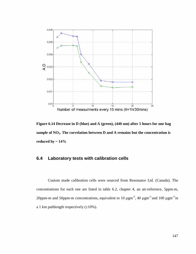
147

Figure 6.14 Decrease in D (blue) and A (green), (440 nm) after 5 hours for one bag

sample of NO2. The correlation between D and A remains but the concentration is

reduced by ~ 14%

6.4 Laboratory tests with calibration cells

Custom made calibration cells were sourced from Resonance Ltd. (Canada). The

concentrations for each one are listed in table 6.2, chapter 4, an air-reference, 5ppm-m,

20ppm-m and 50ppm-m concentrations, equivalent to 10 µgm-3

, 40 µgm-3

and 100 µgm-3

in

a 1 km pathlength respectively (±10%).

148

Cell concentration.

Equivalent for 1m path length

10km path length Concentration error %

1 Atmospheric air 0 ppb 0

2 5ppm-m 0.5ppb ±10

3 20ppm-m 2ppb ±10

4 50ppm-m 5ppb ±10

Table 6.2 (reproduced table 4.2) Concentrations of calibration cells for 1m in the

laboratory (in ppm) and a 10km pathlength (in ppb) equivalent to those that can be

measured in the atmosphere

The bench top setup was rearranged to accommodate the cells. This included an adjustable

clamp to lightly hold each one by its stem for each measurement. Figure 6.15 shows the

new setup with the lenses and optical fibres aligned on either side.

149

Figure 6.15 Calibration cell between source (transmitting lens and fibre) and detector

(receiving lens and fibre) on the optical bench. The cells small size and stem allows

precise alignment for each test.

The atmospheric air cell was used as a reference to determine the absorption of each

NO2 cell sample and this data was examined for correlation with the differential absorption

for the other cells. The cell absorption results made it possible to accurately determine the

concentration and the results were within a small percentage of the concentrations specified

by the supplier. Figure 6.16 illustrates the absorption of each cell. The spectra data are

normalised by subtraction to zero absorption at 499 nm where there are no absorption

features. Note, the absorption features of NO2 are visibly present in the measurement of the

cell with the lowest concentration 5 ppm in 1 m.

Receiving

lens and

fibre

Transmitting

lens and fibre Calibration cell

150

Figure 6.16 Absorption of each calibration cell using the USB4000 spectrometer Note

the increase in size of the absorption features for increasing concentration.

This lowest concentration is equivalent to 1 µgm-3

in 1 km which provides an

excellent example of what the LOD of the novel instrument is, these results were

determined using the USB4000 spectrometer.

6.5 Comparison of each spectrometer for determination of

differential absorption

Comparisons of each spectrometer are possible with the calibration cells because

the concentrations are known. The USB2000 Ocean Optics spectrometer was used for the

first set of laboratory tests. Figure 6.17 illustrates the result of tests on the three cells. The

151

results show a good correlation between A and D with each cell. Calculations using these A

values to determine the concentrations resulted in values close to the concentrations

provided by the manufacturer. It was found that the correlation of A and D could be

affected by the wavelengths chosen in the analysis and the spectrometer being used for the

tests. The air-reference sample cell was used to determine D without NO2 and the result

suggest a low value for absorption but this appears to be within the margin of error for each

measurement.

Figure 6.17 Results of A and D at 440 nm determined from USB2000 spectrometer

results for each cell sample. There is a good correlation between the two sets of results

but D has larger error bars than those for A.

The Maya spectrometer was initially chosen because it had much better low

light level results than the USB2000, which would make it ideal for twilight measurements

in the field, but the concentration results were always below what was predicted, as shown

in figure 6.18. The results of the concentrations determined using both the Maya2000 and

the USB4000 are shown in table 6.3. The expected values for each cell are also shown for

152

comparison. There was also an offset in the measurement of the wavelengths of each peak

of the calibration lamp. This was likely an effect of the etalon features described in chapter

4 that are caused by the Maya’s Back Illuminated CCD structure. This offset could be

corrected in the analysis once the magnitude of the wavelength difference was found using

the calibration lamp. The results show how much lower the Maya2000 concentrations were

compared to the expected results and the USB4000. The results for the absorption

determined using the USB4000 were also slightly less than those predicted, so the

experiment was repeated for 10 sample tests (figures 6.22 to 6.23) and compared to D for

each test.

USB4000, µgm-3

Maya2000, µgm-3

Expected results, µgm-3

0 0 0

2.75 x 105

1.75 x 105 6.5 x 10

5

2.2 x 106 4 x 10

5 2.6 x 10

6

4.75 x 106 1.22 x 10

5 6.5 x 10

6

Table 6.3 Results of cell tests for the USB4000 and the Maya2000

153

Figure 6.18 Absorption at 440 nm for each cell using the Maya2000 (red) compared to

the USB4000 (blue). The Maya2000 results shown are below the results from the

USB4000 and USB2000 this is likely caused by the BI-CCD of the Maya2000.

The USB4000 was ultimately chosen to perform the field measurements

because of its larger resolution. The Maya2000 spectrometer made it easier to identify the

attenuation features but greater accuracy was obtained with the USB spectrometers. The

LOD of the USB4000 was examined using the cells by determining A(λ) and D(λ) at low

light. To test this, an experiment was designed to measure the intensity (digital number, dn)

of light passing through the reference cell and one NO2 cell with a variable NDF (figure

6.19), decreasing the percentage of the intensity in fixed steps.

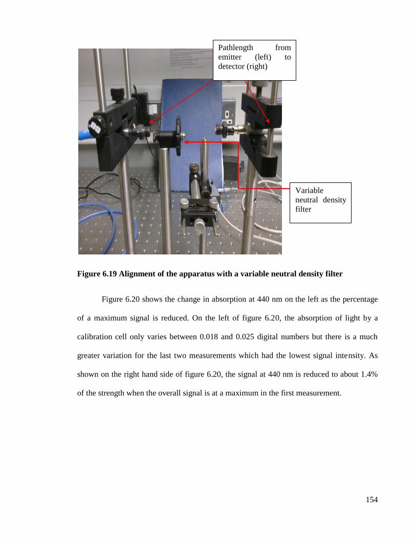
154

Figure 6.19 Alignment of the apparatus with a variable neutral density filter

Figure 6.20 shows the change in absorption at 440 nm on the left as the percentage

of a maximum signal is reduced. On the left of figure 6.20, the absorption of light by a

calibration cell only varies between 0.018 and 0.025 digital numbers but there is a much

greater variation for the last two measurements which had the lowest signal intensity. As

shown on the right hand side of figure 6.20, the signal at 440 nm is reduced to about 1.4%

of the strength when the overall signal is at a maximum in the first measurement.

Variable

neutral density

filter

Pathlength from

emitter (left) to

detector (right)

155

Figure 6.20 Change in A (440 nm) compared to the percentage of the maximum signal

(left image) as the intensity (right image) is decreased by the NDF. The absorption

(red) has a maximum variation when the max % is below 20%. The signal to noise at

this low intensity is very low at the 440 nm feature.

6.6 Absorption and differential absorption determined using the

USB4000

The absorption of each cell at the same wavelength (440 nm) was compared to the

differential absorption for the USB4000 and produced a good correlation between the two,

(figure 6.21). The cell concentration could be determined with greater accuracy, as the

manufacturer provides concentration values within a 10% error so the scale of the A(λ) and

D(λ) values can be predicted. In figure 6.21, the absorption and DOAS are compared for

156

each cell. The results of both methods show an excellent correlation which demonstrates

the accuracy of the Matlab algorithm developed for the analysis. The value for D at 0 ppb-

km represents the error in the DOAS calculation applied to a reference measurement with

no NO2 present. The values for D are offset by 0.0015 to account for variations in the

chosen wavelengths. The accuracy of the results is improved by increasing the number of

measurements. In figure 6.21, the errorbars represent the standard deviation of n=10

measurements on each sample. The absorption without NO2 is taken as 0 ppb-km and the

lowest concentration is 5 ppb in one kilometre which is equivalent to 5 ppm in one metre.

Table 6.4 shows the results of the concentrations calculated from the experimental results

compared to the expected results for the concentrations prepared by the manufacturer of the

cells. The percentage difference for each result is within the 10% error claimed by the

manufacturer.

Figure 6.21 Correlation between A and D (440 nm) for each cell using the USB4000

spectrometer. These results demonstrate the effectiveness of the algorithm and the

accuracy of the technique. DOAS data offset due to variation in chosen wavelengths.

157

USB4000, µgm-3

Percentage

difference between

the two as a %

Expected results, µgm-3

0 0 0

6.75 x 105

3.7 6.5 x 105

2.845 x 106 8.6 2.6 x 10

6

6.425 x 106 1.2 6.5 x 10

6

Table 6.4 Results of cell tests in µgm-3

for the USB4000 (N=10), the percentage

differences are within the 10% parameter claimed by the manufacturer

Analysis of the results of D using the calibration cells is shown in figure 6.22 with a

fitted line that shows how linear the data was. The slope of the line is 4.6x10-4

and the R2

value for the mean is 0.9913 which indicates a strong correlation between the mean of each

measurement of each cell when tested 10 times.

Figure 6.22 Cell concentration and D (440 nm) for n=10 tests on each cell. This shows

the good repeatability of the measurements performed in the laboratory.

158

6.7 Initial measurements of the urban atmosphere to determine

NO2 concentration with the novel-DOAS

The apparatus used to monitor the atmospheric NO2 concentrations was designed to

measure a collimated beam of light using the small uv/vis lens attached to a collimating

tube with an adjustable aperture to manually control the light entering the system, (see

chapter 4 figure 4.10), as too much light directly received by the spectrometer would

saturate the signal. The collimated design was necessary to ensure that the light was

received from a single collimated beam and not from a wide beam that may include

numerous reflections, and interfering sources. Figure 6.25 shows the design of the novel

instrument that was attached to a rotational stage (below the collimating tube). The stage

was then fixed to an adjustable camera stand which was ideal for ensuring the instrument

stayed portable and controllable. The receiving optics can be directed to 1800 in the vertical

plane and 3600 azimuthal. The setup shown in figure 6.25 is light, easy to use and portable.

Attachments to increase the weight can easily be added in high winds and the whole system

has a footprint of two square meters.

159

Figure 6.23 Novel-DOAS apparatus with camera stand. Close-up of collimating tube

and 2m long optical fibre with mini-spectrometer and laptop

Initial tests of the spectrometer outside the laboratory were conducted in

conjunction with the commercial DOAS apparatus on the roof of Kevin St. DIT. Figure

6.26(b) shows the smaller aperture fixed to the top of the commercial system’s receiver

with the aim of detecting the light emitted from the Cathal Brugha St. DIT source located

1.8 km to 2 km (see figure 6.26(a)) away, north of Kevin St. The emitter on the roof of

Cathal Brugha St. was difficult to view from Kevin St. even with binoculars because of the

Spire monument on O’Connell St., constructed after the emitter and detector were installed.

160

Figure 6.24(a) View from Cathal Brugha St. and (b) novel and commercial systems on

Kevin St. roof. Note path in (a) passes between the Spire and Central Bank.

The spectrum of the Xenon lamp used by the OPSIS system, detected by a USB

2000 spectrometer, is shown in figure 6.27. The figure shows samples of two spectra over

the 430 nm to 500 nm wavelength range. In commercial DOAS applications, the lamp and

solar spectrum (blue) are divided by the lamp spectrum (red) and the result is a total

absorption spectrum used to determine the NO2 concentrations. As can be seen in the

image, the spectrum of the 150 Watt lamp contains several distinctive peaks. However, at

(a) The Path from the emitter

to Kevin St. lay between the

Spire and Central Bank

(b) Collimated system

attached to top of DOAS

receiver

161

460 nm, the small peak in the lamp spectrum (red) is difficult to observe in the lamp and

solar spectrum (blue). For the Active DOAS analysis, this spectrum is divided into the

measured spectrum of the light beam projected between the lamp and the spectrometer. For

passive DOAS, only the solar spectrum is needed. An example of a solar spectrum recorded

by the USB4000 is shown in figure 6.28, with an inset of wavelengths 340 to 460 nm.

Because the Cathal Brugha Street lamp had to traverse a pathlength of

approximately 2 km to Kevin Street, the beam could not be detected by the USB

spectrometer. Attempts were also made to detect the Xe lamp at night and low light levels

and with varying integration times, but these were also unsuccessful.

Figure 6.25 Spectra of Xe lamp (red) and lamp and Sun (blue) between 430 to 500 nm

obtained from Cathal Brugha Street.

Peak in lamp spectrum (red) is no longer visible when lamp

spectrum is measured outside

(blue)

162

Figure 6.26 Solar spectrum with inset of 340 to 460 nm features recorded using the

USB4000 spectrometer

Recommissioning the commercial system to measure NO2 over a fixed pathlength

proved to be beyond the capability of the project funding. The system required new

software, calibration and possibly new components. The location of the monitor was not

ideal and removing it would also involve the relocation of the datalogger and controller

unit. An EPA CL monitor was used as an alternative system for comparisons of the NO2

measurements made by the portable instrumentation, see chapter 5 for more detail. The

nearest EPA monitor to Kevin Street was on Wynnefield Rd. in Rathmines, south of Dublin

city centre. Figure 6.29 shows the monitoring site at Wynnefield Rd. at the top of an old

public toilet building.

163

Figure 6.27 Location of EPA monitor in Rathmines. The red circle highlights the inlet

tubes for the monitors.

6.8 Calibration of the in-situ novel-DOAS instrument with

calibration cells

Early tests to calibrate the system involved placing bags containing different

concentrations in front of the instrument which proved to be difficult largely due to the

refraction of the light in each bag and the size of the bags compared to the instrument. The

results of this test are shown in figure 6.30. The value for the concentration is larger with

the NO2-bags than with the no bag measurement, but there was very little difference

between the bag containing only air and those with NO2.

164

Figure 6.28 Variation of concentration when PP bags are placed in front of the

detector. The first point on the graph represents the concentration without a bag.

The calibration cells were also used to test the accuracy of the algorithm used, to

calculate D and the concentration of NO2. Each calibration cell was placed in front of the

aperture. It was expected that the value determined for D would increase as the cells with

higher concentration were placed into the pathlength. The first cell has atmospheric air

content, and could possibly show some variation compared to a D recorded without a cell

present, but this measurement eliminates any error caused by light scattering in the cell.

The variation expected would most likely be due to reflections from the quartz structure of

the cell. The order of the cells in front of the collimator was 5 ppm-m, 20 ppm-m and 50

165

ppm-m. Figure 6.31 shows the results of this test and the change in D value for each

atmosphere+cell measurement. On the x-axis, the numbers 1-5 represent the atmosphere,

atmospheric cell and each cell concentration of NO2 respectively. The results were recorded

five times each to gain an average and standard deviation this would account for any subtle

variations in the pathlength due to light scattering etc. The results confirm the aim of the

research that the wavelengths and the NO2 absorption feature at 440 nm can accurately

identify changes in the NO2 concentration within the instruments optical pathlength for an

average integration time of 5 s.

Figure 6.29 Increasing D for 5 measurements (1) no-cell, (2) air-cell and each

calibration cell (3-5) containing NO2 with ambient sunlight as a source. The results

show that the increase in concentration from each subsequent sample results in an

increase in absorption relative to the difference in concentration.

166

If the value for D in figure 6.31 for the Sun-no cell and atmospheric–air cell are

taken as 0 the increase of approximately 0.003 for the next sample represents the 5 ppm/m

cell. The next sample (20 ppm/m) should be 4 times greater at ~0.012 and the last cell (50

ppm/m) 10 times greater at ~0.03. The results show that the actual absorption increases is

as much as ~0.011 and ~0.025 respectively, indicating that the increase in D can be

attributed to the increasing sample concentrations place in front of the detector.

Figure 6.32 illustrates how D varies throughout the day when each cell is placed in

front of the collimator. The broken blue line represents the changing atmosphere without a

cell present, so the variation should represent atmospheric NO2, and the broken red line

represents the atmospheric air cell. There is very little difference between the two as in

figure 6.31 which suggests that the cell itself has very little effect on the DOAS calculation.

In figure 6.32, seven measurements were taken using each cell every hour between 11am

and 5pm. The green line in figure 6.32 represents the 5 ppm-m concentration, which is

equivalent to 10 µgm-3

/1km which is near the values of the atmospheric air measurements.

This implies that this cell concentration provides a relatively low increase to the

atmospheric NO2. The red and black lines indicate the changing D for the 20 ppm-m and 50

ppm-m cells which are equivalent to concentrations of 40 µgm-3

and 100 µgm-3

in 1 km

respectively. The measurements were taken during daylight hours 11 am to 5 pm, the

overall variation for each cell clearly shows that the DOAS method can detect variations of

NO2 throughout the day under clear sky conditions. Although the results for the low

concentration cell also demonstrate that very small variations in the atmospheric NO2 may

be difficult to distinguish using the DOAS method on overcast days.

167

Figure 6.30 Diurnal variation of D for the atmosphere (blue) and each cell over a

period of 6 hours. Note each NO2 cell has a consistently higher D than the no-cell and

air-cell data.

6.9 Measurements of NO2 in urban environments and

comparison to EPA-CL data

Initial attempts using the novel-DOAS setup were made from the roof top of the

DIT-FOCAS building. Concentrations of NO2 recorded by the EPA were then obtained at

the end of the summer in 2010. Further data was collected using the USB4000 for the

summer of 2011 and compared to the corresponding EPA data for the same dates and times.

As the EPA data is recorded using a CL instrument, discrepancies between the two sets of

data obtained are expected but it is hoped that an average discernible concentration for NO2

may be found for a reasonable comparison of the two technologies (see section 5.3). The

168

factors affecting a good comparison include the measurement approach of each method, the

CL monitor is placed in-situ, with the inlet tube located ~ 2 metres above the ground,

whereas the DOAS instrument records spectra from the roof of the FOCAS building or

from the second floor laboratory. The zenith measurements were taken from the streets near

the CL monitor’s location. Meteorological conditions can also affect the novel-DOAS

measurements as cloudy days cause more scattering of the Sunlight as it passes through the

atmosphere, which causes large variations in the optical pathlength [70, 111]. As explained

in chapter 5 the transportation of NO2 gas in the atmosphere can result in a more dynamic

NO2 variation than that expected from NO2 photolysis and traffic congestion levels

[111](section 5.5).

The DOAS data could be recorded automatically for several days. However, only

the daylight hours were used for analysis and comparison as the signal at low light levels

was too low to perform the DOAS calculation on without errors. The earliest results

showed large variations in the D when 435 nm was used as the central wavelength for the

DOAS calculations. This feature was close to a prominent Fraunhofer feature, so the

smaller feature near 440 nm was used instead.

Each spectrum was dark subtracted and normalised for analysis. Figure 6.33 shows

a comparison between the absorption determined using a horizontal measurement and a

zenith reference (blue) and spectrum of the absorption cross section determined by Bogumil

(green, 2003) corrected by 2 x 1017

. The determination of the absorption using this method

was used by Morales and Walsh (with an S2000 spectrometer) in their paper, which was the

foundation behind this work[5].

169

Figure 6.31 Absorption of Sunlight with zenith reference measurement and α (x

2x105) determined by Bogumil_2003. Although there are NO2 absorption features

visible (at 440 nm) in the zenith reference measurement (blue), this zenith spectrum

will still contain traces of atmospheric NO2.

6.9.1 Correlation of novel-DOAS determined concentrations with EPA

data

The concentration of the DOAS measurements were determined by estimation of

the pathlength (L~ 10 km) based on the estimates of the height of the pollution boundary

layer and the viewing geometry of the spectrometer and collimator. Additional estimates

were made from the similarities between D to the pattern of the EPA data. The diurnal

variation of NO2 in most of the field results is comparable to the SCD variation described in

section 2.9.3. Overall the results show some correlation between the two sets of data for

170

clear bright days. However there is data shown here where the correlation was weak most

likely due to topographical and meteorological variations in the local atmosphere, but it is

possible to make comparisons as shown in figure 5.4. In figure 6.34, the rise in NO2

concentration at the beginning of the day and later (after 4 pm) is characteristic of the

diurnal variation of NO2 due to rush hour traffic congestion. In the example of the results

comparing the DOAS measurement and EPA data shown, the concentrations are still

relatively low with the maximum concentration determined by the EPA being slightly

higher than 4 ppb, which is equivalent to ~7.52 µgm-3

.

Figure 6.32 Variation of the concentration for NO2 in ppb for 26/05/11 (L~10 km)

Initial measurements of the D of scattered sunlight at 435 nm and 440 nm were

performed using the USB2000 spectrometer with a 600 µm fibre-optic. The concentration

of NO2 was then determined from the results and estimates of the pathlength based on the

viewing geometry, see chapter 3. Measurements were made to determine the variation of D

171

for different elevation angles of the front end optics. Figure 6.35 illustrates the variation of

D with changing angle θ. The angle 00 represents the zenith view and 90

0 the horizon. The

gradual increase in D suggests more absorption of the sunlight in the lower troposphere

compared to the upper troposphere and lower stratosphere.

Figure 6.33 Variation of D with a changing elevation angle θ. An increase in D when

the USB4000 is nearly parallel to the horizon suggests higher NO2 concentrations

closer to the Earth’s surface.

This is representative of the higher concentrations of pollutants such as NO2

produced by human activity. To determine the variation of D in different directions the

instrument optics were directed at the available paths in the north, south, east and west

azimuthal directions. These measurements were taken from the roof of the DIT/FOCAS

institute where most of the East view was blocked by the top floor structure and the view

172

directly north was the rear of the DIT Kevin Street building. However, the results in figure

6.36 show that the variation of D for each azimuth was less than 0.02 when each

measurement was taken within a few minutes of each other. It would be expected that

larger variation between each direction would exist, depending on the sources of NO2 in

each direction and on days with higher winds which will affect the lateral transport of the

NO2. The highest concentrations would be expected for the north-east direction towards the

city centre and dockland area, especially during times of day when traffic congestion is

high [11].

Figure 6.34 Variation of D for different azimuthal directions the values for D range

between 0.078 and 0.088.

Measurements were also obtained of the optical pathlength south of the DIT-

FOCAS building on Camden Row. The data was analysed for a variation in D that

compared well with results in the literature [17] and the results obtained for the CL

instrument located within the pathlength. The NO2 feature at 440 nm was used to perform

173

the analysis with the differential absorption cross section (λ)’ = 2.6 x 10-19

cm2/molec.

(3.4 x 10-7

m2µg

-1). The pathlength was again estimated as 10 km and the results were

compared to the data provided by the EPA. The measurements were recorded for full days

between 9 am and 6 pm, weekends from Fridays to Mondays or for several week days. Any

data recorded at night or at twilight were eliminated because there was no sunlight or there

was not enough sunlight to determine an accurate D i.e. the signal was at the limits of

detection (LOD).

Directing the collimator towards the zenith in theory measures the lower

troposphere and some of the stratosphere. The variation of NO2 concentration in the

stratosphere typically has a pattern where the concentration is high in the morning and

evening. The reasons for this variation include the increase in tropospheric concentrations

at this time due to traffic congestion and the reduction in photolytic reactions during

twilight hours when there is less direct sunlight on the Earth’s surface. Some of the results

from these tests are shown in figures 6.37 and 6.38.

174

Figure 6.35 Variation in concentration for zenith directed measurements. There is

higher concentration before 9am in the morning which can indicate high NO2

concentrations from chemical mixing at twilight and morning rush hour traffic.

Figure 6.36 Variation in concentration for zenith directed measurements. As in figure

6.37 the data shows a high value for concentration in the early hours of the day and

slight rise in the evening.

175

6.9.2 Results of comparison of novel-DOAS with EPA

chemiluminescence

As described in chapter 5, section 5.5 there have been successful attempts

comparing in-situ DOAS results to CL measurements. To test the effectiveness of the

measurements made by the proposed novel-DOAS instrument the results obtained from the

analysis were compared to results obtained using CL monitors. In figure 6.39, the blue data

represents the concentration determined using the DOAS method and the red is the

variation of NO2 in Rathmines determined by an EPA CL instrument. The concentrations

determined using DOAS were calculated using estimates of the average pathlength on the

three days 02-04 June 2011. A pathlength of 6 km was estimated for each day. There is

some correlation in the pattern of the data but the DOAS data shows less variation as can be

seen in the peak in NO2 recorded by the EPA in the late afternoon of June 3rd

. This could be

explained by the fact that the DOAS data represents the average NO2 over a path of ~6 km

unlike the CL data which can be influenced by local sources such as nearby traffic

congestion. In the case of the Rathmines location, the traffic sources include a local school,

and the car park in the adjacent apartment block. There is a rise in the NO2 in both sets of

data in the latter half of the each day most likely due to increased congestion.

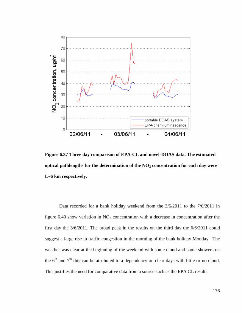
176

Figure 6.37 Three day comparison of EPA-CL and novel-DOAS data. The estimated

optical pathlengths for the determination of the NO2 concentration for each day were

L~6 km respectively.

Data recorded for a bank holiday weekend from the 3/6/2011 to the 7/6/2011 in

figure 6.40 show variation in NO2 concentration with a decrease in concentration after the

first day the 3/6/2011. The broad peak in the results on the third day the 6/6/2011 could

suggest a large rise in traffic congestion in the morning of the bank holiday Monday. The

weather was clear at the beginning of the weekend with some cloud and some showers on

the 6th

and 7th

this can be attributed to a dependency on clear days with little or no cloud.

This justifies the need for comparative data from a source such as the EPA CL results.

177

Figure 6.38 Concentrations of NO2 determined for four days. A single estimated

pathlength of 6 km was used.

As shown in figure 6.39, there can be some correlation between the DOAS method

and local CL data for the overall NO2 concentration throughout the day. But any

correlations in the smaller variations of the data are harder to distinguish because of the

spatial conditions and the variations in the optical pathlength due to light scattering effects.

Figure 6.41 shows similarities between the DOAS and the EPA CL when the average

pathlength is taken as ~ 10 km for each day.

178

Figure 6.39 Comparison of 3 days of DOAS and EPA-CL (L~10 km). For the all three

days the NO2 concentration suggests a good correlation between the two methods.

However, in figure 6.42 the pathlength is estimated to be between 6 km and 10 km

for the weekend of the 1st to the 4

th of July in 2011. The data shown was collected between

8am and 8pm for mostly clear days with light winds. Shorter pathlengths were estimated

for the 1st and 4

th of July which may have been due to an increase in cloud cover and light

showers [93]. The concentrations for the 3/7/2011 show a rise in the afternoon and a large

decrease in NO2 for most of the 4/7/2011 for both methods. The smaller features in the

novel system data could be caused by the actual fluctuations of NO2. But other influences

could be responsible such as the light scattering in the field of view, which could affect the

179

length of L, and the length of time the spectrometer is used e.g. temperature effects on the

dark current. The LOD of the system determined in the laboratory show that the analysis is

capable of identifying concentrations of 10 µgm-3

in 1 km with signal > 20% of the

maximum intensity. But these LOD can vary substantially on cloudy days when the

intensity signal is lower and influenced by electronic noise (figure 6.20).

Figure 6.40 Comparison of 4 days of DOAS and EPA-CL data. (Average pathlength L

~ 8 km) The 3rd

and 4th

of July are similar but small fluctuations in the DOAS data

could be the result of changeable weather conditions.

Comparing the DOAS data for days with very dynamic meteorological conditions

(see sections 1.3 and 2.9.3) demonstrates the effects of light scattering in the atmosphere

and pollution transport have on the DOAS data and NO2 concentrations. The results in

180

figure 6.43(a) show greater differences in NO2 concentration between four different days.

Comparison of the DOAS method and the CL results of the 9th and 10

th of July 2011

requires a large 20 km pathlength estimation. Displayed in 6.43(b) is the comparison of the

novel DOAS system and EPA CL results. A possible reason for the larger pathlength

estimated for the 9th

and 10th

is the changeable meteorological conditions over these few

days. Comparing the weather of the 10th

(L~20 km) and the 11th

(L~6 km) shows that the

10th

had 6 hours of sunshine recorded by Met Eireann whereas the 11th had 8 hours. On the

Monday the 11th

it was mostly dry, with only light breezes, whereas the 10th

was a wet day

with northwesterly winds. The Friday and Monday results are much higher this could be

attributed to traffic emissions caused by increased congestion on weekdays.

Figure 6.41 (a) Variation in NO2 concentration using DOAS (L~6, 20, 20, 6 km)

(b) Comparison of the same data with EPA-CL results

(b) (a)

181

6.9.3 Evaluation of CL and novel-DOAS data

In figure 6.44, the change in NO2 (ppb) recorded by two CL monitors, the EPA

monitor in Rathmines and the Trinity College Dublin Monitor on the roof of DIT Kevin

Street are shown. The change in NO2 recorded by the two CL monitors in different

locations still has a very noticeable correlation. However, the weather on these days was

very changeable, see table 6.5, which would have had more of an effect on the TCD CL

monitor, as it was in a more exposed location and well above the ground. Still, the

correlation between the data obtained from each monitor is enough to demonstrate that

measurements of the average NO2 by remote sensing along a fixed path should provide

comparable results between novel-DOAS and the CL sampling if the atmospheric NO2

concentration was stable. However as figure 6.45 illustrates, the variation of NO2

concentration determined with the DOAS analysis compares poorly with the two CL

monitors, this is attributed to the very dynamic meteorological conditions which can make

remote sensing of NO2 concentration by DOAS very difficult. The pathlengths used for

each day to make the comparison shown are 6, 6, 10 and 8 km respectively, i.e. an average

pathlength of ~7.5 km.

Date Wind Direction Sunshine (national) Weather

29th July NE 5 hours Morning heavy Rain

30th July SE 3 hours Mostly Cloudy

31st

July SW 1 hour Heavy rain, dry evening

1st August Variable 4 hours Cloudy

Table 6.5 Weather for the weekend of 29th

of July to 1st of August 2011

182

Figure 6.42 Change in NO2 concentration in ppb using two CL monitors for the

weekend 29/07 to 02/08 of 2011 (90hrs=3/4days). The overall change in the data

obtained by the two monitors show some correlation which suggests that a CL

monitor is capable of representing an average NO2 concentration in an urban area.

Figure 6.43 Data as shown in figure 6.45 but with the change in NO2 concentration

determined by DOAS (red) added. The estimated pathlengths for each day are L~ 6, 6,

10, 8 km respectively. Heavy showers and dark cloud were also recorded for each

day.

0

5

10

15

20

25

0 20 40 60 80 100

NO

2 p

pb

5pm_29/07 to 9am_02/08 2011

EPA- TCD- Novel DOAS sytem-

183

6.9.4 Further analysis of the EPA and DOAS data comparisons

Figures 6.43 and 6.45 showed how the DOAS data can vary in very different ways

when compared to EPA data. Comparisons of the correlation of these results and others are

shown in figures 6.46 to 6.48. In Figure 6.46, the concentration comparison is shown on the

left and the correlation using a scatter plot on the right. The scatter plot indicates that there

is a slight correlation between the two sets of data but the concentration determined by

DOAS analysis is offset compared to the EPA data, the slope of the line through the plot is

very large at 3.2. The calculated regression constant (R2) for this data gives a good value of

0.539. Figure 6.47 illustrates the data in the same way for the August bank holiday

weekend in 2011. The DOAS data here compares very well with the EPA data with the

slope of line in the scatter plot at 1.3. An R2 value of 0.708 indicates a very good

correlation between each set of data for these four days. In figure 6.49 the slope of the

scatter plot is 4.8 offset largely by the large difference between the EPA and DOAS data

for the 30 of September 2011. The R2 value is very low at 0.094 which indicates an

extremely poor correlation between the DOAS and the CL data. All the DOAS results for

figure 6.48 were calculated with a 10 km pathlength.

184

Figure 6.44 Comparison of in-situ DOAS (blue) and EPA-CL (red) for NO2 and data

correlation 23-25/07/11. The DOAS data is clearly not correlated well with the EPA-

CL data. The slope of the line in the scatter plot is large ~3.2 indicating a weak

correlation between the two methods on these 3 days.

185

Figure 6.45 Comparison of in-situ DOAS (blue) and EPA-CL (red) for NO2 and

correlation 29/07/-01/08/11 the slope of the line in the scatter plot is 1.3 which

indicates a good correlation between each set of data.

186

Figure 6.46 Comparison of in-situ DOAS (blue) and EPA-CL (red) for the

concentration of NO2 and correlation 28-30/09/11 the large difference on the third day

(30/9/11) affects the data giving the line on the scatter plot a slope of 5.4.

187

By comparing the averages of CL and the in-situ novel-DOAS for different days, a

more effective illustration of how the results compare is seen. The larger changes in NO2

concentration demonstrate a much better comparison with each other and the smaller

changes have less influence. Figures 6.49 and 6.50 show that the change in average

concentration for 5 days in September 2011 with an estimated path of 10 km. In figure 6.49

the novel-DOAS data displays the variation in concentration of NO2 in µgm-3

for an

estimated pathlength of 10 km correlates almost exactly with the corresponding EPA data.

This illustrates the effectiveness of the novel-DOAS system in the evaluation of the NO2 in

a local urban atmosphere.

Figure 6.47 Comparison of the average EPA-CL and in-situ novel-DOAS data for 5

consecutive days (L~10 km). There is a clear correlation between both sets of data

obtained by the two different methods.

In figure 6.50, the correlation illustrates less accuracy between the two methods.

The average estimated pathlength for the four days was ~8 km ± 2 km. However, looking at

188

the individual data for each day, figure 6.51 shows that the pattern of the data for the 3rd

and 4th

of July are very similar even with the variation in the estimation of L. These results

are clearly less conclusive than those in figure 6.49. The results make it plain that clear

days provide better correlation between the in-situ novel-DOAS and the EPA-CL because

of the variable pathlength caused by light scattering in the atmosphere by clouds and

variations in the local traffic congestion.

Figure 6.48 Comparison of average CL and in-situ novel-DOAS for 4 days (L~ 6 km

10 km 10 km 6 km respectively). Although there is some comparison in these results

the variation in the estimated pathlength determined by comparing the two sets of

data suggests the results were not conclusive.

189

6.10 Summary

Initial tests were designed to develop the Matlab algorithm and optical arrangement

used to measure NO2 concentrations for samples prepared in the laboratory. Polypropylene

bags were filled with NO and reacted with air already in the bag to form NO2.

Tests results show that an increase in concentration in different bags could be

detected and the D compares with the A. Three different Ocean Optics, miniaturised

spectrometers were used the USB2000, Maya2000 and the USB4000. Ultimately the

USB4000 was chosen for further tests as it had a better resolution and signal to noise

(~22.3 for 500 scans/10 ms) than the others and proved to be the most accurate in

determination of NO2 concentration with lab samples.

The PP bag NO2 concentrations were consistently lower than the expected so

calibration cells with known concentrations were sourced. Comparison of the concentration

calculated from D and A, using the cells were successfully within the 10% error set by the

manufacturer.

Measurements with the USB4000 were performed for several days with the results

showing good correlations particularly for clear days with little changeable weather. The

average results for each method were also compared. The portable system was tested with

the calibration cells and Sunlight illumination by placing the cells in front of the instrument

to determine if there is a change in the calculated novel-DOAS data and each cell was

measured throughout one day and compared to the D variation without a cell. This was to

190

identify any variation due to the cell and if the cell in front of the instrument affected

measurement without the cells.

Tests were performed outside the laboratory using one of the spectrometers and

front end optics constructed to measure different elevation angles and azimuthal directions.

Initial attempts with the OPSIS DOAS system in DIT could not be achieved because of the

state of the OPSIS apparatus and the distance between Kevin St. DIT and Cathal Brugha St.

DIT. An alternative method involved comparing the portable, novel-DOAS instrumentation

to EPA CL. The results obtained show that comparisons can be made between the two

methods but spatial, meteorological differences can affect the strength of any correlation. It

is worth noting that each system the proposed novel-DOAS system and the CL monitor are

designed to meet different accuracy and are expected to vary in their respective locations

and function.

191

CHAPTER 7 Discussion and Conclusions

7.1 Project aims and background

The aim of this research was to develop a novel system for the detection of gaseous

pollutants in an urban environment. The principle of operation of the system was based on

the differential optical absorption spectroscopy (DOAS) method. The novel system

developed in this research is inexpensive, capable of in-situ measurements, is user friendly

and is also capable of comparable measurements with other pollutant detection methods.

The remote sensing technique known as DOAS is based on the principle where

attenuated features in the spectral profile of a broadband source e.g. a tungsten lamp or

Sunlight can be used to determine reference intensity, I0, used to calculate the absorption in

the Beer-Lambert law, see equation 2.10. The DOAS technique uses a variation of the

Beer-Lambert law to determine a differential absorption that is equivalent to absorption

with a reference value denoted by Io’. This value is found mathematically using equation

2.14. With this approach it is possible to determine the concentration of the NO2 gas. Two

forms of the DOAS approach are described in detail in chapter 3 the active and passive

methods using an artificial light source and naturally occurring sunlight respectively.

The active method has been successfully employed in commercial applications

where it records the changes in concentrations for a variety of gases including organic

compounds (VOC), ozone (O3), sulphur dioxide(SO2) as well as NO2 although it is

192

expensive, requires mains power, in some scenarios more than one source, and fixed

constructed locations.

The passive methods on the other hand utilize a variety of approaches including

satellite measurements, plume measurements from smoke stacks and volcano SO2

concentrations with large DOAS devices and miniaturised spectrometers. One of the

objectives of this research is to demonstrate that, with both knowledge of the lower layers

of the atmosphere and concurrent measurements by other instruments, it is possible to

measure NO2 concentrations comparable to local EPA chemiluminescence data using the

novel-DOAS.

7.2 Laboratory work and discussion of the results

To test the validity of the use of a miniaturised spectrometer to measure NO2

concentrations, tests were designed and developed in the laboratory on an optical bench to

determine the correlation of absorption, (A), determined with a reference sample and

differential absorption, (D), where no reference is needed. Along with the spectrometer an

optical fibre coupled to a collimating lens were employed to measure the light passing

through each sample. Using an algorithm developed the mathematical value for Io’ and

hence D were calculated along with a value of A for each sample. The differential

absorption and absorption were plotted against each other and the correlation between the

two was excellent.

Three different miniaturised spectrometers were used; USB2000, Maya2000 with a

back illuminated CCD and a USB4000. Ultimately the USB4000 was chosen which has an

193

optical resolution of ~1.5 nm and dispersion of ~0.18 nm/pixel. Initially PP bags were used

as sample containers but it was discovered the concentrations were below the levels

expected. From the results of measurements on the bags, the concentrations were

approximately 33% of the expected concentrations. These samples were eventually

replaced by custom made calibration cells sources from Resonance Ltd. The results using

the bags showed that there was a good correlation between A and D but the calibration cells

proved to be more accurate with both the correlation of the two values and the

concentrations determined by the algorithm. These cells are more expensive than the bags

but are far less expensive than the commercial DOAS calibration samples. Their small size

also makes them ideal for alignment with the front end optics of the field measurement

configuration i.e. the adjustable aperture and collimating tube, see figures 4.10 and 6.25.

Other tests were performed on the optical bench including a determination of the

differential absorption coefficient, α’, (equation 2.14) for the spectral resolution for the

spectrometer and comparing them to the values described in the literature. A value of 3.4 x

10-7

m2

µg-1

was determined, as the gravimetric equivalent to the absorption cross section

’as an accurate value for the NO2 molecule and is similar to values described in the

literature [4], seen in figure 6.10.

The LOD in the laboratory were also tested for using the smallest concentration

sample which was also comparable to 5 ppm in 1 m (equivalent to 1 µgm-3

in 10 km). A

comparison of a decreasing raw intensity signal was compared to the value of D and A,

determined while the amount of light received was decreased using a variable NDF. The

results of this test showed that D could still be determined with some accuracy even at low

light levels showing that the D was independent of the light intensity level.

194

7.3 Field work results

The final configuration of the novel system consisted of an adjustable aperture

attached to a collimating tube which is coupled to the lens and optical fibre. The fibre is

connected to a USB4000 miniaturised spectrometer which is connected via a USB cable to

a Toshiba laptop. The analysis of the data recorded by the laptop is performed using the

Matlab and SpectraSuite software. The key components are described in table 7.1.

Signal to noise of the USB4000 system, 300:1, was minimised by subtracting the

dark signal from each measurement, see specifications table 7.1. By keeping the signal at a

maximum the effects of electronic noise is reduced. This can be achieved by ensuring the

front end optics is receiving as much light as possible. The integration time for the field

measurements was 500 scans for 10 ms which averaged the signal over 5 seconds and

increases the signal to noise ratio by a factor of ~22. This provides sufficient detector

sensitivity during the day and matches the rate the ambient sunlight changes compared to

commercial DOAS systems which average 30,000 scans over 5 minutes [105].

195

Large scale

dimensions

Stand

height

Collimating tube Aperture maximum Laptop

type

Min: 54

cm

Max: 140

cm

Length: 80 cm

Diameter: 23 mm

23 mm Dell

E6400

Optical

components

Optical

fibre

Length Numerical aperture Diameter

Ocean

Optics

2 m 0.22 600 µm

Lens Focal

length

Optical Range Diameter

Ocean

Optics 10 mm uv/vis

5 mm

Optical

spectrometer

USB4000

CCD S/N No. of pixels Resolution Range

Front

Illuminated

300:1 (increases

√n, n = no. scans)

e.g. 500scans/10

ms √500 → S/N:

~6700

3648 ~1.5 nm

650 nm

(effective

between

200 nm and

1100 nm)

Gas Species

NO2 Limits Of

Detection

Absorption

(visible

range)

Differential

absorption

coefficient α'

Differential

absorption

cross-section σ'

1 µgm-3

/10 km

400 nm -500

nm 3.4x10

-7m

2µg

-1 2.5x10-19

cm2molec

-1

Calibration

Materials

Type Reference Minimum conc. Middle

conc.

Maximum

conc.

Calibration

cells

(Source:

Resonance

Ltd.)

Atmospheric

air

5 ppm-m

(10 µgm-3

–

1 km)

20 ppm-m

(40 µgm-3

–

1 km)

50 ppm-m

(100 µgm-

3–1 km)

Table 7.1 Description of the key components of the final setup of the DOAS device

with the USB4000 spectrometer and calibration cells specifications

196

Zenith measurements using the USB4000 showed that D changes very little in the

middle of the day. It can be high at the beginning and the end of the day, as seen in figures

6.36 and 6.37, most likely due to increased traffic levels as described in the literature

sources. Changing the elevation angle between the zenith and the horizon also reveals a

much higher concentration closer to the horizon. This is expected because of the greater

concentrations of NO2 in the lower atmosphere[6].

Measurements of the atmosphere with the front end optics directed towards the

horizon were conducted from the FOCAS building on Camden Row. Some of these results

are shown in figures 6.41 to 6.42, which illustrate how the concentration varies throughout

the day. Initially attempts were made to compare data obtained from the DIT/DOAS system

described in chapter 5 using methods similar to those described by Dr. Alberto Morales and

Dr. James Walsh in 2005 [5]. It was found, however, that the current DIT system requires

an expensive recalibration and the once available paths are either obstructed by new

buildings or are too long (~ 2 km) to perform an accurate calibration. Ultimately, the results

determined by the novel DOAS system were compared to local CL data provided by the

EPA. These results were compared with the EPA measurements if a reasonable pathlength

of ~10 km is chosen. By comparing the results of the EPA monitor in Rathmines to another

CL monitor placed on the roof of Kevin St. across from FOCAS (figure 6.44 and 6.45), it

was demonstrated that there was a good comparison between the two even though these

sampling monitors were separated by over 1 km. This demonstrates that the results of these

instruments throughout the city are a good representation of the overall average NO2

concentration and therefore it should be possible to gather comparable results with a novel

197

DOAS system which measures the average concentration along a fixed path. Further

comparisons were also made between past EPA data [20].

Further analysis of the correlation of EPA data and the DOAS system demonstrated

that the correlation was much better on clear sunny days. This was most likely due to the

scattering of light long the measured pathlength on cloudy days where the scattered light

can travel through the same part of the atmosphere more than once affecting the

determination of the average NO2. Analysis of the daily average for July and September

2011 (figures 6.49 and 6.50) illustrate how well the EPA data and the novel-DOAS system

can correlate with an approximate pathlength of 10 km.

7.4 Summary of Conclusions

The novel system is constructed from components less expensive (€500) than the

commercial DOAS (€130,000) and CL monitors (€50,000). Overall, the system consisting

of the USB4000 setup costs approximately €3,500 with the front end optics and the four

calibration cells described in chapter 4.

The algorithm developed in Matlab, shown in Appendix II, shows how effective the

absorption data correlates to differential absorption. The value obtained for α’ is the same

as the values given in the literature obtained by other methods.

The portability of the novel system made it possible to record spectra from the roof

tops of the DIT buildings and on the locations in Rathmines. The system can be calibrated

in the laboratory with the cells containing different concentrations of NO2. Calibration can

also be achieved in the field by placing the cells in front of the instrument and calculating

the increases in D for each cell and comparing the results to the D of the open atmosphere.

198

This approach is similar to the methods applied in the COSPEC DOAS application

described in chapter 3. Table 7.2 summarises the conclusions that can be drawn from the

overall research and results.

Laboratory results Field results with novel-DOAS

Excellent correlation between

absorbance (A) and differential

absorption (D) with custom made cells

containing concentrations of NO2

Strong correlation between DOAS

and EPA-CL measurements on clear

days

Absorption coefficient α’ comparable to

values determined from literature

sources

Weak correlation on cloudy days most

likely due to light scattering in the

optical path

Limits of detection ~ 5ppm-m ≡ 1

µgm-3

-10km

Strong correlation of DOAS and

EPA-CL for daily averages

S/N ~22 Portable and adaptable setup

Table 7.2 Comparison of the laboratory and field results obtained with the novel-

DOAS instrument

The results show the effectiveness and accuracy of the measurements in the

laboratory and how the data recorded on clear days in the field is comparable to concurrent

EPA data obtained using CL the existing standard monitoring technique outlined in

European Union policy. The data analysis also compares well with results described in the

literature which was studied in the extensive literature survey conducted at the beginning of

the research.

7.5 Future work

199

The current system could be further developed by developing the algorithm to

include radiative transfer equations to improve the estimation of the L being measured.

Concurrent measurements with local commercial DOAS instruments would be ideal for

correlation as the methodical approach is similar. However correlation with data obtained

from CL monitors could be developed as well as with satellite data to develop a local

profile of the NO2 concentrations in different azimuthal directions and within the UBL of

the troposphere. Further development of the software could also make the system more user

friendly for various operators.

Detection of other pollutants could also be achieved, particularly O3 and SO2 which

are also constantly monitored by the EPA. O3 in particular contributes to the aerosol

measurement data used to determine the AMF and can therefore be useful in the

determination of the vertical height of NO2 concentrations. The results show that cloudy

days have an effect on L by scattering the light passing through the lower atmosphere as a

result meteorological data gathered simultaneously with the DOAS data would add to the

understanding of the pollutant profile.

Alternative designs to the setup could be achieved by the development of a weather

protected casing for the system and an artificial light source like LEDs that would allow

measurements to be undertaken when the light levels are low and during the night. A

modest amount of work has already been achieved with LEDs in this research and in the

literature. In figure 7.1 spectra are shown of the profiles between 300 nm and 600 nm of the

Sun, an LED and the Xenon lamp that could be used for the detection of NO2 in the

laboratory or in the field. However, to be useful for DOAS measurements in the field, the

ideal LED would need to be detectable over a distance of at least 300 m (OPSIS AB), the

200

LED. The commercial DOAS mirror for example produces a very bright, collimated beam,

but does have a disadvantage of size setup of a certain length because of its relatively long

focal length. The CCD miniaturised spectrometers could also be replaced by photodiode

arrays designed to measure the light intensity at specific wavelengths could maximise the

effectiveness of measurements of individual absorption features.

Figure 7.2 Profiles the Light Emitting Diode (green), the Sun (blue) and a Xenon

lamp (black) in the UV/Vis range.

The versatility and variety of applications of the novel-DOAS method shows that it

can be adapted and developed in numerous ways for many applications including the

monitoring of industrial sites, monitoring areas of concentrated traffic congestion and

scientific applications.

201

References:

1. Godish, T., Air Quality. 2004: Lewis Publishers. 460.

2. Association, S.M.H. The vertical structure of the atmosphere. cited 2012;

Available from: http://smha.btck.co.uk/OriginoftheAtmosphere/VerticalStructure.

3. Vandaele 1998, S., Bogumil 2003, Burrows 1998. cited; Available from:

http://www.atmosphere.mpg.de/enid/.../Spectra/Catalogue_Spectra_5p4.html.

4. Morales, J.A. and J.E. Walsh, Detection of atmospheric nitrogen dioxide using a

miniaturised fibre-optic spectroscopy system and the ambient sunlight.

Spectrochimica Acta Part A: Molecular and Biomolecular Spectroscopy, 2005.

61(9): p. 2073-2079.

5. Platt, S., Differential Optical Absorption Spectroscopy: Principles and

Applications. 2008: Wiley.

6. Bird, R.E. and C. Riordan, Simple Solar Spectral Model for Direct and Diffuse

Irradiance on Horizontal and Tilted Planes at the Earth's Surface for Cloudless

Atmospheres. Journal of Climate and Applied Meteorology, 1986. 25(1): p. 87-97.

7. Fisher, B., J. Kukkonen, and M. Schatzmann, Meteorology applied to urban air

pollution problems: COST 715. International Journal of Environment and Pollution,

2003. 16(1-2): p. 560-570.

8. Union, E., Clean Air for Europe (CAFE) Directive. 21st of May 2008

9. API, T. Technical Manual Teledyne Model 200E Nitrogen Oxide Analyser.

Volume,

10. Donnelly, A., B. Misstear, and B. Broderick, Application of nonparametric

regression methods to study the relationship between NO2 concentrations and local

wind direction and speed at background sites. Science of The Total Environment,

2011. 409(6): p. 1134-1144.

11. Driscoll, S.O., On imaging air pollutants in an urban street canyon using

tomographic-DOAS, in Applied Physics and Instrumentation. 2008, Cork Institute

of Technology.

12. Platt, U., Air monitoring by spectroscopic techniques. 1994: Wiley-Interscience.

13. Brauer, M.E.A., air pollution from traffic and the development of respiratory

infections and asthmatic and allergic symptoms in children. American journal

respiratory and critical care medicine, 2002. 166: p. 1092-1098.

202

14. Agency, I.E.P. What we monitor. present cited; Available from:

http://www.epa.ie/whatwedo/monitoring/air/monitor/.

15. Brimblecombe, P., Air composition and chemistry. 2nd ed. Cambridge

environmental chemistry series 6. 1986.

16. Commission, E. Implementation of ambient air quality legislation. 1999 [cited

2012 07-11-2012]; Understanding impact of individual pollutants]. Available from:

http://ec.europa.eu/environment/air/quality/legislation/assessment.htm.

17. Bertram TH, C.R., et al, Consistency of ozone and nitrogen oxides standards at

tropospherically relevant mixing ratios. J Air Waste Manag Assoc, 2005. 55(10): p.

1473-9.

18. Dobson, G.M.B. and D.N. Harrison, Measurements of the amount of ozone in the

earth's atmosphere and its relation to other geophysical conditions. Proceedings of

the Royal Society of London. Series A, 1926. 110(756): p. 660-693.

19. Instrumentation, T.A.P. Instructional Manual: MODEL 300 CARBON MONOXIDE

ANALYZER. Volume, 111

20. Hönninger, G., C. von Friedeburg, and U. Platt, Multi axis differential optical

absorption spectroscopy (MAX-DOAS). Atmos. Chem. Phys., 2004. 4(1): p. 231-

254.

21. Hecht Eugene, Z.A., Optics. 4th ed. 2002, USA and Canada: Addison-Wesley. 565.

22. Boeker, E., van Grondelle, Environmental Physics. 1996: Wiley and Sons. 448.

23. University, W. Identifying elements in the Sun using spectral lines. 2000 2002

[cited; Data description adapted from Learning astronomy by doing astronomy Ana

Larson]. Available from:

http://www.astro.washington.edu/courses/labs/clearinghouse/labs/Solarspec2/sunsp

ec.html.

24. De Beek, R., et al., The Ring effect in the cloudy atmosphere. Geophysical research

letters, 2001. 28(4): p. 721-724.

25. Wagner, T., Correction of the Ring effect and Io effect for DOAS observations of

scattered sunlight.

26. Chance, K.V. and R.J.D. Spurr, Ring effect studies: Rayleigh scattering, including

molecular parameters for rotational Raman scattering, and the Fraunhofer

spectrum. Applied Optics, 1997. 36(21): p. 5224-5230.

27. Schneider, W., Moorgat, G.K., et al, Absorption cross sections of NO2 in the UV

and visible region (200 - 700 nm)at 298 K. Photochem. Photobiol., 1987(40): p.

195-217.

203

28. Bovensmann, H., et al., SCIAMACHY: Mission Objectives and Measurement

Modes. Journal of the Atmospheric Sciences, 1999. 56(2): p. 127-150.

29. Vandaele, A.C., Hermans, C., et al Measurements of the NO2 absorption cross

section from 42000 cm-1

to 10000 cm-1

(238-1000 nm) at 220K and 294K. Journal of

Quantitative Spectroscopy and Radiative Transfer, 1998. 59: p. 171-184.

30. Bogumil, K., Orphal, J., et al Measurements of molecular absorption spectra with

the SCIAMACHY pre-flight model: Instrument characterisation and reference data

for atmospheric remote sensing in the 230-2380 nm region J. Photochem. Photobiol

A: photochemistry, 2003. 157: p. 167-184.

31. Orphal, J., A critical review of the absorption cross-sections of O3 and NO2 in the

ultraviolet and visible. Journal of Photochemistry and Photobiology A: Chemistry,

2003. 157(2–3): p. 185-209.

32. Noxon, J.F., Nitrogen Dioxide in the Stratosphere and Troposphere Measured by

Ground-Based Absorption Spectroscopy. Science, 1975. 189(4202): p. 547-549.

33. Platt, U., D. Perner, and H.W. Pätz, Simultaneous Measurement of Atmospheric

CH2O, O3, and NO2 by Differential Optical Absorption. J. Geophys. Res., 1979.

84(C10): p. 6329-6335.

34. Roscoe, H.K., et al., Intercomparison of slant column measurements of NO2 and O4

by MAX-DOAS and zenith-sky UV and visible spectrometers. Atmos. Meas. Tech.

Discuss., 2010. 3(4): p. 3383-3423.

35. Chan, K.L., et al., NO2 measurements in Hong Kong using LED based long path

differential optical absorption spectroscopy. Atmos. Meas. Tech., 2012. 5(5): p.

901-912.

36. DOAS, U.o.B.I. IUP-Bremen DOAS group. [cited 2008; Summary of DOAS

materials and research conducted by IUP-Bremen, specifically satellite projects].

Available from: http://www.iup.uni-bremen.de/doas/index.html.

37. Van Roozendael, M., et al., Intercomparison of BrO measurements from ERS-2

GOME, ground-based and balloon platforms. Advances in Space Research, 2002.

29(11): p. 1661-1666.

38. Solomon, S., A.L. Schmeltekopf, and R.W. Sanders, On the Interpretation of Zenith

Sky Absorption Measurements. J. Geophys. Res., 1987. 92(D7): p. 8311-8319.

39. Zuo, H., et al., Equiangular method: a technique of multiaxis DOAS. J. Opt. Soc.

Am. B, 2009. 26(8): p. 1656-1662.

40. von Friedeburg, C., et al., Derivation of tropospheric NO3 profiles using off-axis

differential optical absorption spectroscopy measurements during sunrise and

comparison with simulations. J. Geophys. Res., 2002. 107(D13): p. 4168.

204

41. Hendrick, F., et al., Intercomparison exercise between different radiative transfer

models used for the interpretation of ground-based zenith-sky and multi-axis DOAS

observations. Atmos. Chem. Phys., 2006. 6(1): p. 93-108.

42. Iwabuchi, H., Efficient Monte Carlo methods for radiative transfer modelling

Journal of atmospheric sciences, 2006.

43. Wagner, T., et al., Comparison of box-air-mass-factors and radiances for Multiple-

Axis Differential Optical Absorption Spectroscopy (MAX-DOAS) geometries

calculated from different UV/visible radiative transfer models. Atmos. Chem. Phys.,

2007. 7(7): p. 1809-1833.

44. Leigh, R.J., et al., Concurrent multiaxis differential optical absorption spectroscopy

system for the measurement of tropospheric nitrogen dioxide. Appl. Opt., 2006.

45(28): p. 7504-7518.

45. AB, O., AR500 Opto-Analyser. 1993, Furulund, Sweden: Opsis-AB.

46. Obinsk, P.T. Commercial DOAS system. cited; Available from:

eridan.mega.ru/adr.htm.

47. GmbH, H.M. Products. cited; Available from: http://www.hmm.de/.

48. S.A., E. Multi-Gas long path air quality monitoring system. [cited 2012;

Commercial DOAS system France]. Available from:

http://www.environnement.it/public/articoli/53/Files/Sanoa_Scheda_tecnica_uk.pdf.

49. EPA, I., Air Quality in Ireland 2011 key indicators of ambient air quality. 2011,

EPA 2012: Ireland.

50. Aliwell, S.R., et al., Analysis for BrO in zenith-sky spectra: An intercomparison

exercise for analysis improvement. J. Geophys. Res., 2002. 107(D14): p. 4199.

51. Eisinger, M., et al., DOAS Zenith Sky Observations: 1. BrO Measurements over

Bremen (53 N) 1993–1994. Journal of atmospheric chemistry, 1997. 26(1): p. 93-

108.

52. Galle, B., et al., A miniaturised ultraviolet spectrometer for remote sensing of SO2

fluxes: a new tool for volcano surveillance. Journal of Volcanology and Geothermal

Research, 2003. 119(1–4): p. 241-254.

53. Petritoli, A., et al., Off-axis measurements of atmospheric trace gases by use of an

airborne ultraviolet-visible spectrometer. Applied optics, 2002. 41(27): p. 5593-

5599.

54. Bobrowski, N., Honniger, G., Galle, B., Platt, U., Detection of BrO in a volcanic

plume. Nature, 2002. 423(6937): p. 3.

205

55. Melamed, M.L., et al., Detection of pollution transport events southeast of Mexico

City using ground-based visible spectroscopy measurements of nitrogen dioxide.

Atmos. Chem. Phys., 2009. 9(14): p. 4827-4840.

56. Frins, E., et al., Tomographic multiaxis-differential optical absorption spectroscopy

observations of Sun-illuminated targets: a technique providing well-defined

absorption paths in the boundary layer. Appl. Opt., 2006. 45(24): p. 6227-6240.

57. Takashima, H., et al., NO2 observations over the western Pacific and Indian Ocean

by MAX-DOAS on Kaiyo, a Japanese research vessel. Atmos. Meas. Tech.

Discuss., 2011. 4(5): p. 6069-6095.

58. Kramer, L.J., et al., Comparison of OMI and ground-based in situ and MAX-DOAS

measurements of tropospheric nitrogen dioxide in an urban area. J. Geophys. Res.,

2008. 113(D16): p. D16S39.

59. Pfeilsticker, K., et al., Optical path modifications due to tropospheric clouds:

Implications for zenith sky measurements of stratospheric gases. J. Geophys. Res.,

1998. 103(D19): p. 25323-25335.

60. Frins, E., et al., Tomographic MAX-DOAS observations of sun illuminated targets:

a new technique providing well defined absorption paths in the boundary layer.

2006.

61. Vlemmix, T., et al, Potential and limitations of the MAX-DOAS method to retrieve

the vertical distribution of tropospheric nitrogen dioxide. Atmospheric

Measurement techniques discussions, 2011. 4: p. 4013-4072.

62. Richter, A. and J.P. Burrows, Tropospheric NO2 from GOME measurements.

Advances in Space Research, 2002. 29(11): p. 1673-1683.

63. Burrows, J., Dehn, A., et al, Atmospheric remote-sensing reference data from

GOME: part I. Temperature-dependent absorption cross-sections of NO2 in the

231-794 nm range. Journal Quant. Spectroscopic radiation transfer 1998. 60: p.

1025-1031.

64. Streets, D.G., T. Canty, and e. al, Emissions estimation from satellite retrievals: A

review of current capability. Atmospheric Environment, 2013.

65. Boeker, E., van Grondelle, Environmental Physics. 2011: Wiley and Sons. 448.

66. TEMIS. Total and Tropospheric NO2 columns from GOME II. 2013 cited;

Available from:

http://www.temis.nl/airpollution/no2col/no2monthgome2_v2.php?Year=2013&Mo

nth=05.

67. Elias, T., et al., Comparison of COSPEC and two miniature ultraviolet spectrometer

systems for SO&lt;sub&gt;2&lt;/sub&gt; measurements using scattered sunlight.

Bulletin of Volcanology, 2006. 68(4): p. 313-322.

206

68. Aeronomy, B.I.o.S. WinDOAS. 2012 cited 2011; Available from: http://uv-

vis.aeronomie.be/software/WinDOAS/.

69. F. Gotz, A.R.M., G. Dobson, The vertical distribution of Ozone in the Atmosphere.

Proceedings of the Royal Society Series A 1934. 145(855): p. 416-466.

70. Andersen, A.H. and A.C. Kak, Simultaneous Algebraic Reconstruction Technique

(SART): A superior implementation of the ART algorithm. Ultrasonic Imaging,

1984. 6(1): p. 81-94.

71. Louban, I., et al, Measurement of SO2 and NO2 applying ToTaL-DOAS from

remote site. Journal of Optics A: Pure adn Applied Optics, 2008. 10(10).

72. Sinreich, R., et al., Multi axis differential optical absorption spectroscopy (MAX-

DOAS) of gas and aerosol distributions. Faraday discussions, 2005. 130: p. 153-64;

discussion 241-64, 519-24.

73. Sinreich, R., et al., Parameterising radiative transfer to convert MAX-DOAS dSCDs

into near-surface box-averaged mixing ratios. Atmospheric Measurement

Techniques, 2013. 6(6): p. 1521-1532.

74. Cohn, A., Angevine, W.M., Boundary layer height and entrainment zone thickness

measured by lidars and wind-profiling radars. American meteorological society,

2000. 39(8): p. 1233-1247.

75. Halla, J.D., et al., Determination of tropospheric vertical columns of NO2 and

aerosol optical properties in a rural setting using MAX-DOAS. Atmos. Chem.

Phys., 2011. 11(23): p. 12475-12498.

76. Sinreich, R., et al., Parameterising radiative transfer to convert MAX-DOAS dSCDs

into near-surface box-averaged mixing ratios. Atmospheric Measurement

Techniques, 2013. 6(6): p. 1521-1532.

77. Hao-yi, Z., et al., Retrieval of the vertical column density of the atmospheric

pollution gases by using the scattered solar radiation. Journal of Quantitative

Spectroscopy and Radiative Transfer, 2008. 109(15): p. 2628-2634.

78. Williams, E.J., et al., Comparison of Ultraviolet Absorption, Chemiluminescence,

and DOAS Instruments for Ambient Ozone Monitoring. Environmental Science &

Technology, 2006. 40(18): p. 5755-5762.

79. Lamsal, L.N., et al., Ground-level nitrogen dioxide concentrations inferred from the

satellite-borne Ozone Monitoring Instrument. Journal of Geophysical Research,

2008. 113(D16): p. D16308.

80. Wagner, T., et al., Cloudy sky optical paths as derived from differential optical

absorption spectroscopy observations. Journal of Geophysical Research:

Atmospheres, 1998. 103(D19): p. 25307-25321.

207

81. Hertel*, O. and M. Evan Goodsite, Chapter 1 Urban Air Pollution Climates

throughout the World, in Air Quality in Urban Environments. 2009, The Royal

Society of Chemistry. p. 1-22.

82. Online, M.E.T.I.M.S. Climate of Ireland. 2013 cited; Available from:

http://www.met.ie/climate-ireland/climate-of-ireland.asp.

83. Murphy, J.G., S. O'Driscoll, and N.J. Smith, Multipath DOAS for tomographic

measurements. 2003: p. 875-885.

84. Optics, O. Ocean Optics devices. cited; Available from:

http://www.oceanoptics.com.

85. Dooly, G., et al., Low Concentration Monitoring of Exhaust Gases Using a UV-

Based Optical Sensor. Sensors Journal, IEEE, 2007. 7(5): p. 685-691.

86. Fitzpatrick, C., O’Donoghue, C., Lewis, E., A novel multi-point UV optical fibre

sensor based on cladding luminescence. Measurement science and technology,

2003. 14: p. 1477-1483.

87. Chen, D., et al., Tropospheric NO2 column densities deduced from zenith-sky DOAS

measurements in Shanghai, China, and their application to satellite validation.

Atmos. Chem. Phys., 2009. 9(11): p. 3641-3662.

88. Hecht Eugene, Z.A., Optics. 7th ed. 1982, USA and Canada: Addison-Wesley. 565.

89. Hamamatsu. S10420 CCD. cited; Available from:

http://sales.hamamatsu.com/assets/pdf/parts_S/s10420-6_etc_kmpd1102e02.pdf.

90. O'Malley, M.J. and E. O'Mongain, Charge-coupled devices: frame adding as an

alternative to long integration times and cooling. Optical Engineering, 1992. 31(3):

p. 522-526.

91. Scientific, R. Spectroscopic etaloning in back illuminated CCDs. cited 2012;

Summary of Spectroscopic etaloning in BI-CCDs]. Available from:

http://www.roperscientific.de/etaloning.html.

92. Walsh, J.E., et al., Fibre-optic micro-spectrometers for biomedical sensing.

Transactions of the Institute of Measurement and Control, 2000. 22(5): p. 355-369.

93. Ltd, R. Calibration Cells. cited; Available from:

http://www.resonance.on.ca/calibration_cells.htm.

94. instruments, T. Instruction Manual Model 200A Chemiluminescent analyzer.

Volume, 225

95. Morales, J.A., J. Treacy, and S. Coffey, Urban ozone measurements using

differential optical absorption spectroscopy. Analytical and Bioanalytical

Chemistry, 2004. 379(1): p. 51-55.

208

96. Ireland, E.P.A., Air Quality Annual Report 2011, Environment, Editor. 2011:

Ireland.

97. Council, D.C., Air Quality monitoring and noise control Dublin Regional air

quality management plan 2009-2012, D.C. Council, Editor. 2009-2012.

98. Leigh, R.J., et al., Spatially resolved measurements of nitrogen dioxide in an urban

environment using concurrent multi-axis differential optical absorption

spectroscopy. Atmos. Chem. Phys., 2007. 7(18): p. 4751-4762.

99. Dunlea, E.J., et al., Evaluation of nitrogen dioxide chemiluminescence monitors in a

polluted urban environment. Atmos. Chem. Phys., 2007. 7(10): p. 2691-2704.

100. Vlemmix, T,.et.al., MAX-DOAS tropospheric nitrogen dioxide column

measurements compared with the Lotos-Euros air quality model. Atmos. Chem.

Phys., 2011/10/26. 11(10): p. 49.

101. Van Houcke, E., Garland, Wendy and Treacy Jack. Measurement of SO2 in Dublin

City by Differential Optical Absorption Spectroscopy. Facility for Optical

Characterisation and Spectroscopy (FOCAS), Dublin Institute of Technology.

102. Rooney, J., Garland, Wendy and Treacy, Jack. Formaldehyde in urban air. Facility

for Optical Characterisation and Spectroscopy (FOCAS), Dublin Institute of

Technology.

103. Kambe, Y., et al., Monitoring of atmospheric nitrogen dioxide by long-path pulsed

differential optical absorption spectroscopy using two different light paths. Journal

of Environmental Monitoring, 2012. 14(3): p. 944-950.

1

Appendix I Paper submitted for publication to the Atmospheric

Measurement Techniques

Title: A portable spectroscopic detection system for pollution monitoring in an urban

environment.

Brian Devine1 and. James E. Walsh

2

1Optical Sensors and Metrology Laboratory,

FOCAS,

Dublin Institute of Technology,

Camden Row, Dublin 8

2On leave from School of Physics,

College of Sciences and Health

Dublin Institute of Technology

Kevin Street, Dublin 8

Ireland

Currently

Director of Pre-University Studies,

MAHSA University College,

Jalan Universiti Campus,

Jalan Elmo, off Jalan Universiti,

59100 Kuala Lumpur, Malaysia

2

Abstract

Monitoring of air pollutants such as Nitrogen Dioxide (NO2) that are toxic or environmentally

damaging is a key metric for environmental protection agencies worldwide. There is a constant need to

develop new technologies and methodologies that provide real-time, low cost pollution measurements over a

broad range of sampling sites, particularly in urban and industrial areas.

Typically detection of pollutants in urban environments is performed using a variety of techniques

many of which are expensive, require complex setups and are in fixed locations. The novel system presented

here is designed for portable, low cost and in-situ detection of pollutants such as NO2 using Differential

Optical Absorption Spectroscopy (DOAS). The basis for the system is the new generation of miniature fibre

optic spectrometers that provide measurement specifications close to that of more traditional high cost DOAS

instruments which are used to cross calibrate the initial data. The system can also be calibrated against other

NO2 sampling techniques such as chemiluminescence (CL) monitors. Based on laboratory calibration the

final measurement accuracy of the system in the field was less than ± 0.5 ppb over a calibration dynamic

range of 0-50 ppb under typical daylight conditions. This level of accuracy was achieved with repeated

measurements, n=10, of custom made calibration cells containing known concentrations of NO2.

Laboratory experiments using a controlled light source were designed to examine the correlation

between absorption and differential absorption using the calibration cells and a specifically developed

algorithm based on the Beer-Lambert Law. These laboratory calibration tests verified that differential

absorption determined using the novel system can be used to quantify NO2 concentrations both in the

laboratory and in the open atmosphere of a surrounding urban area. Field tests, using ambient sunlight as a

source, were then conducted and compared to concurrent CL measurements. Good correlations have been

confirmed between the novel systems data and the established NO2 quantification methods.

Results prove that low cost fibre optic spectrometer systems can be used to identify and quantify

gaseous pollutants in real-time using ambient sunlight and additional experiments using the new generation of

high intensity light emitting diodes (LED) indicate that future systems can also be based around low cost LED

arrays.

3

1. Introduction

1.1 Air pollution

Modern transport and industrial activities have resulted in the need to monitor gas pollutants

produced in urban environments[21]. Several modern scientific methods have been utilised to accurately

assess concentration levels, among these methods are those that directly sample gases and remote sensing of

the average gas concentration[6]. The work presented here describes the development of a novel optical

sensing system for monitoring gas pollution, based on differential optical absorption spectroscopy (DOAS)

that is portable, inexpensive and will have reduced complexity compared to existing similar systems.

Monitoring the distribution and concentration of pollutants requires an understanding of the

atmosphere, the types of pollutants, and the different methods of detection employed in their quantification.

The atmosphere can be divided into different layers which are characterised by their changes in altitude,

temperature and pressure. The natural composition of the atmosphere is primarily Nitrogen (78%), Oxygen

(21%) and other gases e.g. Argon, CO2, and Water[1, 6]. Natural sources such as volcanoes and plant

decomposition as well as human activities contribute a broad range of gaseous pollutants to the atmosphere

including nitrogen dioxide, sulphur dioxide, formaldehyde and particulate matter[6]. In the urban environment

the primary source of these gasses is man-made and the distribution of pollution concentration throughout an

urban environment and it’s immediate atmosphere is primarily determined by factors such as the location of

the emission sources, time of day and local weather conditions[34].

The optical system described here can technically quantify a broad range of polluting gases in the

atmosphere but has been developed using nitrogen dioxide (NO2) as the primary target test analyte due to its

importance as a primary toxic pollutant and high spectral absorption coefficient at key/convenient visible

wavelengths[5]. Nitrogen dioxide is a reddish brown gas and is present in the atmosphere, typically in the 0-

100 ppb range, as a product of the naturally occurring nitrogen cycle and due to anthropogenic sources

notably combustion[1, 6]. It’s presence in the atmosphere is related to photochemical smog, acid rain and

lower visibility[16] it is also partly responsible for the chemical formation of nitric oxide from photochemical

reactions and the destruction of ozone by oxidation[16]. The standard set limits for the concentration of NO2

in the atmosphere are usually determined by a country’s respective Environmental Protection Agency (EPA),

with EU regulations[9] allowing a mean annual concentration of 40 μg m-3

at 200C, which is roughly 21 ppb.

4

In addition a maximum of 200 μg m-3

may not be exceeded more than 18 times a year as short term spikes in

NO2 will have public health implications[9].

The effect of NO2 on human health includes respiratory complications and airway restrictions. Long-

term exposure can increase the risk of these respiratory issues[112]. NO2 has a lifetime in the atmosphere of

~2 days[6, 113] and known sources of NO2 include the Nitrogen cycle in local eco-systems, industrial

facilities and combustion engines. It is therefore essential that levels of toxic atmospheric gas such as NO2 are

accurately and frequently monitored in populated areas to ensure annual EPA standards are met and to

provide alarm level detection when concentration spikes occur. NO2 levels are also correlated with daily

traffic congestion and industrial activity and can therefore be used as a monitor of urban pollution events by

the EPA.

The accurate detection and monitoring of NO2 concentrations and emissions in the atmosphere are

achieved by a broad range of techniques that include direct sampling of the local atmosphere followed by

chemical analysis in the field or laboratory. Direct sampling followed by optical analysis in a sampling

chamber can be performed by using laser-induced fluorescence[114] or chemiluminescence (CL) and remote

sensing by optical methods such as Differential Optical Absorption Spectroscopy (DOAS)[13]. NO2 levels in

Dublin are monitored by the Irish EPA, according to the EU standards, using a CL technique. A Teledyne

NOx Analyzer, model 200E (Teledyne Advanced Pollution Instrumentation, Cal. U.S.) is an example of the

standard CL device used, it samples the atmosphere through an inlet approximately 2 metres above ground

making it comparable to NOx inhaled by humans[10]. The extracted sample typically contains nitric oxide,

NO, and nitrogen oxides, NOx that are detected by a photomultiplier tube after the sample chemically reacts

with a molybdenum catalytic converter the concentration of NO2 is found by subtraction[10]. Other forms of

NOx detection by CL may vary for different instruments. The method employed for this research is based

solely on DOAS, which is a type of spectroscopy that can use a broad spectrum to detect several pollutants.

This paper describes the design construction and testing of a novel, low cost DOAS system based around a

fibre optic spectrometer system that overcomes many of the problems of the existing standard methods.

5

1.2 Atmospheric absorption spectroscopy

The absorption of electromagnetic radiation as a function of wavelength is a result of the

interaction of the radiation with absorbing molecules in the path of the radiation. The chemical identity of an

absorbing molecule can be determined from the unique spectral fingerprint it produces at specific

wavelengths in the spectrum of incident radiation. Most absorption spectroscopy techniques require a

reference spectrum of the test medium and the illuminating light source with no absorbing analyte present. If

the reference spectrum is denoted by I0() and the measurement spectrum with absorbing analyte present

denoted by I(), the sample absorption (A) is defined as:

A() = log(I0 ()/I ()) (1)

The Beer-Lambert Law then relates A(l) to key analyte metrics as follows:

A(l) = α()cL (2)

Where L is the optical path-length (m), c is the analyte concentration (kg.m-3

) and is α is the analyte specific

absorption coefficient (m2kg

-1) which is determined from the absorption cross section[5], σ, in cm

2molecule

-1.

6

Figure 1 Absorption coefficient as a function of wavelength for NO2 with spectral features of specific

interest to this research highlighted [41, 43, 75].

For a known path-length analyte concentration is therefore directly related to specific absorption features in

the absorption spectrum whose spectral fingerprint is contained in the specific absorption coefficient curve

shown in fig. 1[41, 43, 75].

1.3 Differential optical absorption spectroscopy

In certain environmental monitoring situations, such as Tropospheric NO2 quantification, it is very

difficult to make a representative measurement of the reference intensity, I0, as it requires a measurement

virtually the same atmospheric path-length with no target analyte present. The DOAS method, developed in

the 1970’s by Noxon[46] and Platt[47], overcomes this by determining a differential absorption (D) at the

selected target analyte fingerprint wavelengths in the measured spectrum. The principle behind the DOAS

algorithm for the NO2 spectral feature near 440 nm is shown in fig. 2, with the related calculations for

determining the differential absorption, D, given equations. 3 to 5. The reference value used in the calculation

of I0’(l) is related to the mean of the non absorbing regions either side of the analyte absorbing wavelength at

I2(l), and the final values of D should be equivalent to absorption, A(l), values calculated using the reference

Io curve if available.

7

Figure 2 Comparison of reference (blue) and measured spectra (green) with labelled intensities of an

attenuated feature used in the determination of D.

I0’= I1+ ((I2-I1) (λ2- λ1/ λ3- λ1)) (3)

I = I2 (4)

D = log (I0’/I) (5)

D () = α’ () cL (6)

The absorption coefficient α is wavelength dependent so a differential α’ is approximated to be ~ 3.4

x 10-7

m2μg

-1 for wavelength range of 350nm-500nm, see eq. (6). The concentration of the NO2 is given in

units of μgm-3

as specified by EU regulations alternatively the units can be in volumetric ratio ppm or ppb.

DOAS systems can be used to determine profiles of gases such as NO2 and BrO in the local

atmosphere using Multi-Axis DOAS or MAX-DOAS[32]. The MAX-DOAS measurements are more versatile

than the commercial DOAS as miniaturised spectrometers are used and no artificial light source is required

they are also comparable to other detection methods such as satellite measurements. However MAX-DOAS

8

may only provide data for column densities in molecules/m2 and the cost and mobility of the instruments is

limited when more than one detector is used for simultaneous measurements of different elevation angles.

One miniaturised portable spectrometer was used the USB4000 available from Ocean

Optics[95]. The detection of NO2 in the lower atmosphere above Dublin city involved the calculation of D

from the recorded spectra with an algorithm designed in Matlab and a rigorously designed and tested optical

set up. This system is demonstrated here to be portable, inexpensive and adaptable to a variety of applications

e.g. traffic monitoring, location study, area surveys and continuous monitoring using ambient solar light and

light emitting diodes.

2 Experimental: The novel detection system

The device will ideally will be portable and more affordable than the larger commercial DOAS

system. The design will include optical components that maximise the light from various artificial and natural

sources it will use a lens and collimating tube connected to the micro-spectrometer via an optical fibre. The

following are proposed features of the system:

1. A narrow Field Of View, FOV. The FOV is the 3-Dimensional fraction of the area of the atmosphere

viewed by the sytsems front end optics. The detector used for this research required a FOV with a

comparable pathlength to a larger commercial DOAS system. The FOV should be parallel as too much

divergence of the field can affect the volume being measured.

2. An adjustable aperture fixed to the collimating tube for a parallel FOV and to allow the measurement

of a dark signal, which is subtracted to remove dark current and electronic noise, as the detected signal

varies over time. The length of the collimating tube will also determine the field of view and the

overall size of the detector.

3. A lens and fibre to detect enough light for a maximum signal. The sizes and spectral range of the lens

and fibre must be compatible with the chosen wavelength range being investigated and the range of the

spectrometer. These optical components will also need to detect light of the same wavelength emitted

by broadband artificial sources.

4. A micro-spectrometer with a spectral resolution determined by the CCD detector and the width of the

entrance slit. A bandwidth that allows the user to examine the detected signal for features that can be

9

used for the DOAS calculation eqns. 3-5. The spectrometer will need a wavelength range where

features of NO2 are present (350 nm to 550 nm). The spectrometer needs to have a signal to noise ratio

and limits of detection comparable to larger DOAS system. The detection of real time spectra also

requires the system to have a fast processing speed determined by a combination of the spectrometer

and the laptop it’s connected to.

The novel system has been developed so that it is comparable to the methods used by typical DOAS

techniques. Its novel design will make it less accurate however, ’The design characteristics therefore have to

be a compromise between flexibility and maximising the signal to noise’, J.E. Walsh et al[103].. The

USB4000 uses a Toshiba TCD1304AP CCD linear array also with a 25µm slit 3648 pixels and S/N of 300:1.

The range of detection for the USB4000 is approximately 200nm-850nm and a FWHM of 1.5nm. The

USB4000 with the optical fibre and front end optics arrives at a much lower cost than that of a larger

commercial system.

2.1 Laboratory tests

The laboratory tests involved custom made quartz cells manufactured by Resonance Ltd[104], the

cells were filled with known concentrations of NO2 and one cell contained atmospheric air making it ideal as

a reference. Each cell could be placed within a collimated beam of light, produced by a tungsten lamp the

light is collimated by optical fibres and lenses directing the light beam through the sample. The receiving lens

and fibre are coupled to the spectrometer. The complete apparatus is shown in fig. 3. The advantages of the

calibration cells included the known concentrations provided by the manufacturer and the comparable

concentrations to the expected NO2 in equivalent pathlengths through the atmosphere. They are small, high

quality quartz cells with a two year shelf life that have a diameter of 22mm and a thickness of 14.3mm with a

stem. They are ideal for placing in front of the collimating lens and the adjustable aperture of the front end

optics used in the field. From the experimental data the results obtained were used to determine the limits of

detection and signal to noise (S/N) of the measurements. The spectrometer collected the light with a 5mm

collimating lens and a 600µm diameter optical fibre. Integration times of 10ms for 100 scans and 500 scans

10

were used for the laboratory testing, the integration time of averages 5 scans per second. With these

integration times the S/N increases by ~22.3.

A reference sample was used with other samples containing different concentrations of NO2. Both A

and D were determined from the measured spectra of these samples and the results compared. The spectral

region for NO2 absorption is between 330nm and 500nm with prominent features at 435nm and 441nm, the

detection limits for NO2 in the atmosphere are 0.2ppb for a 5km path length at 200C [6]. The features at

435nm although suitable for the laboratory tests were too close to a prominent Fraunhofer line in the solar

spectrum however the 441nm feature proved adequate. Early testing showed a good correlation between D

determined for each sample without the reference and A were results were calculated with the reference

sample which are shown in fig. 5. The Ocean Optics USB4000 spectrometer operates with SpectraSuite

software which controls the integration time and number of scans as well as displaying the spectra. D and A

were calculated using the purposely written Matlab algorithm.

Figure 3 Calibration cell between source and detector (Main picture) on the optical bench. The cells

small size and stem allows precise alignment for each test (inset)

USB4000

spectrometer

NO2 cell sample

11

The limit of detection of the technique was determined using the cells and showed that the

cell with the lowest concentration 5ppm-m or 6.7 x 105µgm

-3 for 1.4cm cell was close to the minimum

detectable limit of the system, this was equivalent to 0.94µgm-3

in a 10km path as described in table 1 section

3.1.

2.2 Field Tests

Measurements taken with the spectrometer were of the atmosphere directly overhead i.e. the zenith

direction and across the Dublin skyline at elevation angles ranging from 00 parallel to the ground to 30

0 (fig.

4). Measurements made from the FOCAS institute laboratory were of the sky above the south of Dublin city.

For when the weather was not suitable to place the detector outside so the collimating tube and the aperture

were adjusted to eliminate any reflections and light from within the room.

The recorded spectra were used to determine the differential absorption (D) of 438nm to 443nm to

determine a value for D in eq. (5). Approximate pathlengths determined from the literature were10 km [5, 69]

for the horizontal and 1km for zenith measurements of the planetary boundary layer. These were used to

calculate the concentrations see figs. 5-7.

Measurements with the calibration cells involved placing the cells in front of the adjustable aperture

at the end of the 100mm collimating tube starting with the atmospheric air sample. The expected results

should show an increase in D for each cell except the air sample and the differences in magnitude between the

increases should correspond to the differences in concentration between the cells, see fig. 10. For example the

50ppm-m cell would not show an increase less than that expected by the 5ppm-m cell when each one was

placed in front of the detector.

12

Figure 4: Novel-DOAS apparatus with camera stand, collimating tube, adjustable aperture (close up in

inset) and 2m long optical fibre with (Maya2000) mini-spectrometer and laptop

3. Results and Discussion:

3.1.1 Laboratory Results

The cells concentrations including the reference cell filled with atmospheric air and three cells with

different concentrations of NO2 are shown in table 1.

Cell concentration. Equivalent for

1 metre path length.

1km

Production Error %

1 Atmospheric Air 0ppb 0

2 5ppm-m 5ppb ±10

3 20ppm-m 20ppb ±10

4 50ppm-m 50ppb ±10

Table 1: Concentrations of Calibration Cells over 1m and equivalent over 1km

The results in fig. 5 were obtained when each cell was tested 10 times and the results plotted with

errors because of the low concentration of the 5ppm-m cell it was ideal for an approximate determination of

the limits of detection of the system. The concentrations in fig. 5 are shown in ppb-km to illustrate the scale of

the cell concentration in relation to a commercial DOAS pathlength. The small size and stem of the cells

13

made it possible to place them in a lens holder in front of the detector for atmospheric measurements in the

field.

Figure 5: Correlation between A and D for each calibration cell using the USB4000 spectrometer.

These results demonstrate the effectiveness of the algorithm and the accuracy of the technique.

Figure 6 Cell concentration and D for n=10 tests on each cell. This shows the good repeatability of the

measurements performed in the laboratory.

14

The values for A and D were determined using the path through the cell and the differential

absorption coefficient α’ was calculated to be ~3.4e-7 m2µg

-1. The result of the tests in the laboratory with the

tungsten-halogen lamp show there is a very good correlation between A and D (fig. 5). For each of the cells

the measured concentration fell within the manufacturer’s error of 10%. Therefore limits of detection showed

that the system was capable of detecting concentrations of close to 0.5ppb in a 10km path, in fig. 6 the

accuracy of the laboratory tests performed on each cell is determined using a regression line with R2 value of

0.9913.

3.1.2 Detection of NO2 in the atmosphere

Figure 7 Increasing D for 5 measurements (1) no-cell, (2) air-cell and each calibration cell (3-5)

containing NO2 with ambient sunlight as a source.

Measurements of the atmosphere with the custom made cells placed in front of the detector

throughout any day (fig. 7) show that the increase in NO2 concentration to the path being measured is

detectable by the DOAS method and the relative differences between the increases in concentration are

comparable to the differences between the cells (fig. 5) once the outside concentration without the cells is

subtracted. This is ideal for calibrating the system when measuring the local atmosphere.

15

Measurements of the atmosphere above DIT buildings were performed from the FOCAS building

and from the roof of Kevin Street DIT. Fig.8 shows typical data taken for four consecutive days using the

DOAS method with results compared with measurements made by a CL monitor placed in the path of the

novel system. These results are inconclusive as the weather was cloudy and wet and not ideal for

measurements of ambient sunlight. Clouds cause scattering effects which can vary the optical path of the light

being measured[71]. However there is some correlation for an estimated pathlength of 5 km.

Figure 8 Four day comparison of EPA-CL and DOAS data. The estimated optical pathlengths for the

determination of the NO2 concentration for each day were l~5 km respectively.

Further comparisons of the DOAS method and CL reveal differences in data with sharp changes in

the atmospheric NO2 measured by CL. Fig. 9 illustrates how the data from each method compares. These

results were obtained on a clearer day, although there are differences between CL and the DOAS techniques

particularly that the CL is a point sampling technique which can be affected by local traffic congestion and

the DOAS results are subject to variations in the optical pathlength by meteorological and topographical

variations. A scatter plot of the data for late July 2011, (fig. 10), reveals that some correlation exists and by

fitting a line to the data the slope is 1.3 which suggests the variation in NO2 determined by CL and the novel

DOAS are comparable between the two sets of recorded data for concentrations ranging between 5 µgm-3

and

25 µgm-3

. A correlation factor (R2) obtained was very good at 0.708. The larger differences are likely due to

16

the differences in the types of measurement i.e. point sampling and remote sensing and the differences in the

levels accuracy of each method.

Figure 9 Comparison of in-situ DOAS and EPA for the concentration of NO2 and correlation 30/07/11

to 01/08/11

Figure 10 Scatter plot of the same data presented in fig. 8 with slope 1.3 and a correlation factor of R2 =

0.708.

17

4. Conclusions

4.1 Summary of the results

To test the validity of the use of a miniaturised spectrometer to measure NO2 concentrations, tests

were designed and developed in the laboratory on an optical bench to determine the correlation of absorption,

(A), determined with a reference sample and the differential absorption, (D), were no reference is needed.

Using an algorithm developed the mathematical value for Io’ and hence D were calculated along with a value

of A for each sample the results show that the correlation between the two was excellent. A value of 3.4 x 10-

7 m

2 µg

-1 was determined for the absorption coefficient, α’. This was found to be an accurate value for the α’

for NO2 similar to values described in the literature [41]. The limits of detection were determined in the

laboratory using the smallest concentration sample which was also comparable to 5 ppm in 1 m (equivalent to

1 µgm-3

in 10 km).

The final configuration of the novel system consisted of an adjustable aperture attached to a

collimating tube which is coupled to the lens and optical fibre. The fibre is connected to a USB4000

miniaturised spectrometer which is connected via a USB cable to a Toshiba laptop. The analysis of the data

recorded by the laptop is performed using the Matlab and SpectraSuite software. The integration time

for the field measurements 500 scans/10 ms which averaged the signal over 5 seconds increases the signal to

noise ratio by a factor of ~22.

The results can be compared with the EPA measurements if a reasonable pathlength of ~10 km is

chosen. Further analysis of the correlation of EPA data and the DOAS system demonstrated that the

correlation was much better on clear sunny days. Figure 10 illustrates how well the EPA data and the DOAS

system can correlate with an approximate pathlength of 10 km.

The novel system is constructed from relatively inexpensive components far less expensive than the

commercial DOAS and CL monitors. The portability of the novel system made it possible to record spectra

from the roof tops of the DIT buildings and on the locations in Rathmines. The system can be calibrated in the

18

laboratory with the cells containing different concentrations of NO2. Calibration can also be achieved in the

field by placing the cells in front of the instrument and calculating the increases in D for each cell and

comparing the results to the D of the open atmosphere. The results show that the effectiveness and accuracy

of the measurements on clear days in the field is comparable to concurrent EPA data obtained using CL the

existing standard monitoring technique outlined in European Union policy.

4.2 Future Work

Concurrent measurements with local CL monitors could be taken with satellite data to develop a

local profile of the NO2 concentrations in different azimuthal directions and within the troposphere. Further

development of the software could make the system more user friendly for various operators. Cheap

alternative light sources would make the system more versatile allowing measurements to be taken at night

and under various meteorological conditions.

Detection of other pollutants could also be achieved particularly O3 and SO2 which are also

constantly monitored by the EPA. O3 in particular contributes to the aerosol measurement data used to

determine the AMF and can therefore be useful in the determination of the vertical height of NO2

concentrations.

Acknowledgements

EPA STRIVE Research Program Grant

1

References:

1. Godish, T., Air Quality. 2004: Lewis Publishers. 460.

2. E.U., Clean Air for Europe (CAFE) Directive. 21st of May 2008 European Union.

3. Association, S.M.H. The vertical structure of the atmosphere. [cited 2012;

Available from: http://smha.btck.co.uk/OriginoftheAtmosphere/VerticalStructure.

4. Vandaele 1998, S., Bogumil 2003, Burrows 1998. [cited; Available from:

http://www.atmosphere.mpg.de/enid/.../Spectra/Catalogue_Spectra_5p4.html.

5. Morales, J.A. and J.E. Walsh, Detection of atmospheric nitrogen dioxide using a

miniaturised fibre-optic spectroscopy system and the ambient sunlight.

Spectrochimica Acta Part A: Molecular and Biomolecular Spectroscopy, 2005.

61(9): p. 2073-2079.

6. Platt, S., Differential Optical Absorption Spectroscopy: Principles and

Applications. 2008: Wiley.

7. Bird, R.E. and C. Riordan, Simple Solar Spectral Model for Direct and Diffuse

Irradiance on Horizontal and Tilted Planes at the Earth's Surface for Cloudless

Atmospheres. Journal of Climate and Applied Meteorology, 1986. 25(1): p. 87-97.

8. Fisher, B., J. Kukkonen, and M. Schatzmann, Meteorology applied to urban air

pollution problems: COST 715. International Journal of Environment and Pollution,

2003. 16(1-2): p. 560-570.

9. Union, E., Clean Air for Europe (CAFE) Directive. 21st of May 2008

10. API, T. Technical Manual Teledyne Model 200E Nitrogen Oxide Analyser.

Volume,

11. Donnelly, A., B. Misstear, and B. Broderick, Application of nonparametric

regression methods to study the relationship between NO2 concentrations and local

wind direction and speed at background sites. Science of The Total Environment,

2011. 409(6): p. 1134-1144.

12. Driscoll, S.O., On imaging air pollutants in an urban street canyon using

tomographic-DOAS, in Applied Physics and Instrumentation. 2008, Cork Institute

of Technology.

13. Platt, U., Air monitoring by spectroscopic techniques. 1994: Wiley-Interscience.

14. Brauer, M.E.A.e.a., Air pollution from traffic and the development of respiratory

infections and asthmatic and allergic symptoms in children. American journal

respiratory and critical care medicine, 2002. 166: p. 1092-1098.

15. Agency, I.E.P. What we monitor. present [cited; Available from:

http://www.epa.ie/whatwedo/monitoring/air/monitor/.

16. Brimblecombe, P., Air composition and chemistry. 2nd ed. Cambridge

environmental chemistry series 6. 1986.

17. EPA, I., Air Quality in Ireland 2011 key indicators of ambient air quality. 2011,

EPA 2012: Ireland.

18. Commission, E. Implementation of ambient air quality legislation. 1999 [cited

2012 07-11-2012]; Understanding impact of individual pollutants]. Available from:

http://ec.europa.eu/environment/air/quality/legislation/assessment.htm.

2

19. Ireland, E.P.A., Air Quality Annual Report 2011, Environment, Editor. 2011:

Ireland.

20. Council, D.C., Air Quality monitoring and noise control Dublin Regional air

quality management plan 2009-2012, D.C. Council, Editor. 2009-2012.

21. Holloway, A., Wayne, R, Atmospheric Chemistry, ed. R. publishing. 2010: RSC.

22. Harrison, R.M., Hester, R.E., Hertel, Ole, Air Quality in urban environments. 2009:

Royal Society of Chemistry.

23. Wayne, R.P., Chemistry of the Atmosphere. 2000: Oxford University Press Inc.

24. instruments, T. Instruction Manual Model 200A Chemiluminescent analyzer.

Volume, 225

25. Bertram TH, C.R., et al, Consistency of ozone and nitrogen oxides standards at

tropospherically relevant mixing ratios. J Air Waste Manag Assoc, 2005. 55(10): p.

1473-9.

26. Dobson, G.M.B. and D.N. Harrison, Measurements of the amount of ozone in the

earth's atmosphere and its relation to other geophysical conditions. Proceedings of

the Royal Society of London. Series A, 1926. 110(756): p. 660-693.

27. Instrumentation, T.A.P. Instructional Manual: MODEL 300 CARBON MONOXIDE

ANALYZER. Volume, 111

28. AB, O., AR500 Opto-Analyser. 1993, Furulund, Sweden: Opsis-AB.

29. Cohn, A., Angevine, W.M., Boundary layer height and etrainment zone thickness

measured by lidars and wind-profiling radars. Amercian meteorological society,

2000. 39(8): p. 1233-1247.

30. Harren, F.J.M., et al., Photoacoustic spectroscopy in trace gas monitoring.

Encyclopedia of Analytical Chemistry, 2000.

31. Courtillot, I., et al., Sub-ppb NO2 detection by optical feedback cavity-enhanced

absorption spectroscopy with a blue diode laser. Applied Physics B, 2006. 85(2-3):

p. 407-412.

32. Hönninger, G., C. von Friedeburg, and U. Platt, Multi axis differential optical

absorption spectroscopy (MAX-DOAS). Atmos. Chem. Phys., 2004. 4(1): p. 231-

254.

33. Hecht Eugene, Z.A., Optics. 4th ed. 2002, USA and Canada: Addison-Wesley. 565.

34. Boeker, E., van Grondelle, Environmental Physics. 1996: Wiley and Sons. 448.

35. University, W. Identifying elements in the Sun using spectral lines. 2000 2002

[cited; Data description adapted from Learning astronomy by doing astronomy Ana

Larson]. Available from:

http://www.astro.washington.edu/courses/labs/clearinghouse/labs/Solarspec2/sunsp

ec.html.

36. De Beek, R., et al., The Ring effect in the cloudy atmosphere. Geophysical research

letters, 2001. 28(4): p. 721-724.

37. Wagner, T., Correction of the Ring effect and Io effect for DOAS observations of

scattered sunlight.

38. Chance, K.V. and R.J.D. Spurr, Ring effect studies: Rayleigh scattering, including

molecular parameters for rotational Raman scattering, and the Fraunhofer

spectrum. Applied Optics, 1997. 36(21): p. 5224-5230.

39. Francis Rouessac, A.R., Chemical Analysis, modern instrumental methods and

techniques 2000: John Wiley & sons.

3

40. E Haller, H.K., L.S. Cederbaum, The visible absorption spectrum of NO2: A three-

mode nuclear dynamics investigation Journal of Molecular spectroscopy, 1985.

111(2): p. 377-397.

41. Schneider, W., Moorgat, G.K., et al, Absorption cross sections of NO2 in teh UV

and visible region (200 - 700 nm)at 298 K. Photochem. Photobiol., 1987(40): p.

195-217.

42. Bovensmann, H., et al., SCIAMACHY: Mission Objectives and Measurement

Modes. Journal of the Atmospheric Sciences, 1999. 56(2): p. 127-150.

43. Vandaele, A.C., Hermans, C., et al Measurements of the NO2 absorption cross

section from 42000 cm-1

to 10000 cm-1

(238-1000 nm) at 220K and 294K. Journal of

Quantitative Spectroscopy and Radiative Transfer, 1998. 59: p. 171-184.

44. Bogumil, K., Orphal, J., et al Measurements of molecular absorption spectra with

the SCIAMACHY pre-flight model: Instrument characterisation and reference data

for atmospheric remote sensing in the 230-2380 nm region J. Photochem. Photobiol

A: photochemistry and photobiology, 2003. 157: p. 167-184.

45. Orphal, J., A critical review of the absorption cross-sections of O3 and NO2 in the

ultraviolet and visible. Journal of Photochemistry and Photobiology A: Chemistry,

2003. 157(2–3): p. 185-209.

46. Noxon, J.F., Nitrogen Dioxide in the Stratosphere and Troposphere Measured by

Ground-Based Absorption Spectroscopy. Science, 1975. 189(4202): p. 547-549.

47. Platt, U., D. Perner, and H.W. Pätz, Simultaneous Measurement of Atmospheric

CH2O, O3, and NO2 by Differential Optical Absorption. J. Geophys. Res., 1979.

84(C10): p. 6329-6335.

48. Roscoe, H.K., et al., Intercomparison of slant column measurements of NO2 and O4

by MAX-DOAS and zenith-sky UV and visible spectrometers. Atmos. Meas. Tech.

Discuss., 2010. 3(4): p. 3383-3423.

49. Chan, K.L., et al., NO2 measurements in Hong Kong using LED based long path

differential optical absorption spectroscopy. Atmos. Meas. Tech., 2012. 5(5): p.

901-912.

50. DOAS, U.o.B.I. IUP-Bremen DOAS group. [cited 2008; Summary of DOAS

materials and research conducted by IUP-Bremen, specifically satellite projects].

Available from: http://www.iup.uni-bremen.de/doas/index.html.

51. Van Roozendael, M., et al., Intercomparison of BrO measurements from ERS-2

GOME, ground-based and balloon platforms. Advances in Space Research, 2002.

29(11): p. 1661-1666.

52. Solomon, S., A.L. Schmeltekopf, and R.W. Sanders, On the Interpretation of Zenith

Sky Absorption Measurements. J. Geophys. Res., 1987. 92(D7): p. 8311-8319.

53. Zuo, H., et al., Equiangular method: a technique of multiaxis DOAS. J. Opt. Soc.

Am. B, 2009. 26(8): p. 1656-1662.

54. von Friedeburg, C., et al., Derivation of tropospheric NO3 profiles using off-axis

differential optical absorption spectroscopy measurements during sunrise and

comparison with simulations. J. Geophys. Res., 2002. 107(D13): p. 4168.

55. Hendrick, F., et al., Intercomparison exercise between different radiative transfer

models used for the interpretation of ground-based zenith-sky and multi-axis DOAS

observations. Atmos. Chem. Phys., 2006. 6(1): p. 93-108.

56. Iwabuchi, H., Efficient Monte Carlo methods for radiative transfer modelling

Journal of atmospheric sciences, 2006.

4

57. Wagner, T., et al., Comparison of box-air-mass-factors and radiances for Multiple-

Axis Differential Optical Absorption Spectroscopy (MAX-DOAS) geometries

calculated from different UV/visible radiative transfer models. Atmos. Chem. Phys.,

2007. 7(7): p. 1809-1833.

58. Leigh, R.J., et al., Concurrent multiaxis differential optical absorption spectroscopy

system for the measurement of tropospheric nitrogen dioxide. Appl. Opt., 2006.

45(28): p. 7504-7518.

59. Obinsk, P.T. Commercial DOAS system. [cited; Available from:

eridan.mega.ru/adr.htm.

60. GmbH, H.M. Products. [cited; Available from: http://www.hmm.de/.

61. S.A., E. Multi-Gas long path air quality monitoring system. [cited 2012;

Commerical DOAS system France]. Available from:

http://www.environnement.it/public/articoli/53/Files/Sanoa_Scheda_tecnica_uk.pdf.

62. Aliwell, S.R., et al., Analysis for BrO in zenith-sky spectra: An intercomparison

exercise for analysis improvement. J. Geophys. Res., 2002. 107(D14): p. 4199.

63. Eisinger, M., et al., DOAS Zenith Sky Observations: 1. BrO Measurements over

Bremen (53 N) 1993–1994. Journal of atmospheric chemistry, 1997. 26(1): p. 93-

108.

64. Galle, B., et al., A miniaturised ultraviolet spectrometer for remote sensing of SO2

fluxes: a new tool for volcano surveillance. Journal of Volcanology and Geothermal

Research, 2003. 119(1–4): p. 241-254.

65. Petritoli, A., et al., Off-axis measurements of atmospheric trace gases by use of an

airborne ultraviolet-visible spectrometer. Applied optics, 2002. 41(27): p. 5593-

5599.

66. Bobrowski, N., Honniger, G., Galle, B., Platt, U., Detection of BrO in a volcanic

plume. Nature, 2002. 423(6937): p. 3.

67. Melamed, M.L., et al., Detection of pollution transport events southeast of Mexico

City using ground-based visible spectroscopy measurements of nitrogen dioxide.

Atmos. Chem. Phys., 2009. 9(14): p. 4827-4840.

68. Frins, E., et al., Tomographic multiaxis-differential optical absorption spectroscopy

observations of Sun-illuminated targets: a technique providing well-defined

absorption paths in the boundary layer. Appl. Opt., 2006. 45(24): p. 6227-6240.

69. Takashima, H., et al., NO2 observations over the western Pacific and Indian Ocean

by MAX-DOAS on Kaiyo, a Japanese research vessel. Atmos. Meas. Tech.

Discuss., 2011. 4(5): p. 6069-6095.

70. Kramer, L.J., et al., Comparison of OMI and ground-based in situ and MAX-DOAS

measurements of tropospheric nitrogen dioxide in an urban area. J. Geophys. Res.,

2008. 113(D16): p. D16S39.

71. Pfeilsticker, K., et al., Optical path modifications due to tropospheric clouds:

Implications for zenith sky measurements of stratospheric gases. J. Geophys. Res.,

1998. 103(D19): p. 25323-25335.

72. Frins, E., et al., Tomographic MAX-DOAS observations of sun illuminated targets:

a new technique providing well defined absorption paths in the boundary layer.

2006.

73. Vlemmix, T.E.A., et al, Potential and limitations of the MAX-DOAS method to

retrieve the vertical distribution of tropospheric nitrogen dioxide. Atmospheric

Measurement techniques discussions, 2011. 4: p. 4013-4072.

5

74. Richter, A. and J.P. Burrows, Tropospheric NO2 from GOME measurements.

Advances in Space Research, 2002. 29(11): p. 1673-1683.

75. Burrows, J., Dehn, A., et al, Atmospheric remote-sensing reference data from

GOME: part I. Temperature-dependent absorption cross-sections of NO2 in the

231-794 nm range. Journal Quant. Spectroscopic radiation transfer 1998. 60: p.

1025-1031.

76. Streets, D.G., T. Canty, and e. al, Emissions estimation from satellite retrievals: A

review of current capability. Atmospheric Environment, 2013.

77. Boeker, E., van Grondelle, Environmental Physics. 2011: Wiley and Sons. 448.

78. TEMIS. Total and Tropospheric NO2 columns from GOME II. 2013 [cited;

Available from:

http://www.temis.nl/airpollution/no2col/no2monthgome2_v2.php?Year=2013&Mo

nth=05.

79. Elias, T., et al., Comparison of COSPEC and two miniature ultraviolet spectrometer

systems for SO&lt;sub&gt;2&lt;/sub&gt; measurements using scattered sunlight.

Bulletin of Volcanology, 2006. 68(4): p. 313-322.

80. Aeronomy, B.I.o.S. WinDOAS. 2012 [cited 2011; Available from: http://uv-

vis.aeronomie.be/software/WinDOAS/.

81. F. Gotz, A.R.M., G. Dobson, The vertical distribution of Ozone in the Atmosphere.

Proceedings of the Royal Society Series A 1934. 145(855): p. 416-466.

82. Andersen, A.H. and A.C. Kak, Simultaneous Algebraic Reconstruction Technique

(SART): A superior implementation of the ART algorithm. Ultrasonic Imaging,

1984. 6(1): p. 81-94.

83. Louban, I., et al, Measurement of SO2 and NO2 applying ToTaL-DOAS from

remote site. Journal of Optics A: Pure adn Applied Optics, 2008. 10(10).

84. Sinreich, R., et al., Multi axis differential optical absorption spectroscopy (MAX-

DOAS) of gas and aerosol distributions. Faraday discussions, 2005. 130: p. 153-64;

discussion 241-64, 519-24.

85. Sinreich, R., et al., Parameterising radiative transfer to convert MAX-DOAS dSCDs

into near-surface box-averaged mixing ratios. Atmospheric Measurement

Techniques, 2013. 6(6): p. 1521-1532.

86. Halla, J.D., et al., Determination of tropospheric vertical columns of NO2 and

aerosol optical properties in a rural setting using MAX-DOAS. Atmos. Chem.

Phys., 2011. 11(23): p. 12475-12498.

87. Sinreich, R., et al., Parameterizing radiative transfer to convert MAX-DOAS dSCDs

into near-surface box-averaged mixing ratios. Atmospheric Measurement

Techniques. 6(6): p. 1521-1532.

88. Hao-yi, Z., et al., Retrieval of the vertical column density of the atmospheric

pollution gases by using the scattered solar radiation. Journal of Quantitative

Spectroscopy and Radiative Transfer, 2008. 109(15): p. 2628-2634.

89. Williams, E.J., et al., Comparison of Ultraviolet Absorbance, Chemiluminescence,

and DOAS Instruments for Ambient Ozone Monitoring. Environmental Science &

Technology, 2006. 40(18): p. 5755-5762.

90. Lamsal, L.N., et al., Ground-level nitrogen dioxide concentrations inferred from the

satellite-borne Ozone Monitoring Instrument. Journal of Geophysical Research,

2008. 113(D16): p. D16308.

6

91. Wagner, T., et al., Cloudy sky optical paths as derived from differential optical

absorption spectroscopy observations. Journal of Geophysical Research:

Atmospheres, 1998. 103(D19): p. 25307-25321.

92. Hertel*, O. and M. Evan Goodsite, Chapter 1 Urban Air Pollution Climates

throughout the World, in Air Quality in Urban Environments. 2009, The Royal

Society of Chemistry. p. 1-22.

93. Online, M.E.T.I.M.S. Climate of Ireland. 2013 [cited; Available from:

http://www.met.ie/climate-ireland/climate-of-ireland.asp.

94. Murphy, J.G., S. O'Driscoll, and N.J. Smith, Multipath DOAS for tomographic

measurements. 2003: p. 875-885.

95. Optics, O. Ocean Optics devices. [cited; Available from:

http://www.oceanoptics.com.

96. Dooly, G., et al., Low Concentration Monitoring of Exhaust Gases Using a UV-

Based Optical Sensor. Sensors Journal, IEEE, 2007. 7(5): p. 685-691.

97. Fitzpatrick, C., O'Donoghue, C., Lewis, E., A novel multi-point UV optical fibre

sensor based on cladding luminescence. Measurement science and technology,

2003. 14: p. 1477-1483.

98. Chen, D., et al., Tropospheric NO2 column densities deduced from zenith-sky DOAS

measurements in Shanghai, China, and their application to satellite validation.

Atmos. Chem. Phys., 2009. 9(11): p. 3641-3662.

99. Hecht Eugene, Z.A., Optics. 7th ed. 1982, USA and Canada: Addison-Wesley. 565.

100. Hamamatsu. S10420 CCD. [cited; Available from:

http://sales.hamamatsu.com/assets/pdf/parts_S/s10420-006_etc_kmpd1102e02.pdf.

101. O'Malley, M.J. and E. O'Mongain, Charge-coupled devices: frame adding as an

alternative to long integration times and cooling. Optical Engineering, 1992. 31(3):

p. 522-526.

102. Scientific, R. Spectroscopic etaloning in back illuminated CCDs. [cited 2012;

Summary of Spectroscopic etaloning in BI-CCDs]. Available from:

http://www.roperscientific.de/etaloning.html.

103. Walsh, J.E., et al., Fibre-optic micro-spectrometers for biomedical sensing.

Transactions of the Institute of Measurement and Control, 2000. 22(5): p. 355-369.

104. Ltd, R. Calibration Cells. [cited; Available from:

http://www.resonance.on.ca/calibration_cells.htm.

105. Morales, J.A., J. Treacy, and S. Coffey, Urban ozone measurements using

differential optical absorption spectroscopy. Analytical and Bioanalytical

Chemistry, 2004. 379(1): p. 51-55.

106. Leigh, R.J., et al., Spatially resolved measurements of nitrogen dioxide in an urban

environment using concurrent multi-axis differential optical absorption

spectroscopy. Atmos. Chem. Phys., 2007. 7(18): p. 4751-4762.

107. Dunlea, E.J., et al., Evaluation of nitrogen dioxide chemiluminescence monitors in a

polluted urban environment. Atmos. Chem. Phys., 2007. 7(10): p. 2691-2704.

108. Vlemmix, T.E.A.e.a., MAX-DOAS tropospheric nitrogen dioxide column

measurements compared with the Lotos-Euros air quality model. Atmos. Chem.

Phys., 2011/10/26. 11(10): p. 49.

109. Van Houcke, E., Garland, Wendy and Treacy Jack. Measurement of SO2 in Dublin

City by Differential Optical Absorption Spectroscopy. Facility for Optical

Characterisation and Spectroscopy (FOCAS), Dublin Institute of Technology.

7

110. Rooney, J., Garland, Wendy and Treacy, Jack. Formaldehyde in urban air. Facility

for Optical Characterisation and Spectroscopy (FOCAS), Dublin Institute of

Technology.

111. Kambe, Y., et al., Monitoring of atmospheric nitrogen dioxide by long-path pulsed

differential optical absorption spectroscopy using two different light paths. Journal

of Environmental Monitoring, 2012. 14(3): p. 944-950.

112. EPA, U.S. Air nitrogen oxides health. [cited; Available from:

http://www.epa.gov/air/nitrogenoxides/health.html.

113. Velders, G.J.M., et al., Global tropospheric NO2 column distributions: Comparing

three-dimensional model calculations with GOME measurements. J. Geophys. Res.,

2001. 106(D12): p. 12643-12660.

114. Miyazaki, K., et al., Development of atmospheric NO analyzer by using a laser-

induced fluorescence NO2 detector. Atmospheric Environment, 2008. 42(33): p.

7812-7820.

1

Appendix II Matlab algorithm used for data analysis

% DOAS and EPA-CL data analysis %load drk3.txt load drk1.txt wv=drk1(:,1); drk1=drk1(:,2); drk=(drk1+drk2+drk3)./3; load scope00.txt scope00=scope00(:,2);

nmspec=471;

%loads scope10 to scope540 text files for i=10:nmspec;

eval(['load scope',num2str(i),'.txt']); i; end %assigns scope files 0-9 to 'array' for i=1:9;

eval(['array(:,',num2str(i),')=scope0',num2str(i),'(:,2);']); end %assigns scope files 10-540 to 'array' for i=10:nmspec;

eval(['array(:,',num2str(i),')=scope',num2str(i),'(:,2);']); i; end

wvnrm=20:40; for i=1:nmspec;

eval(['arrayd(:,',num2str(i),')=array(:,',num2str(i),')-( (drk1) .*

(mean(array(wvnrm,',num2str(i),') ) )./mean(drk1(wvnrm)) );']); i; end

%DOAS calculation b1=1129; %438 nm p1=1137; %440 nm b2=1149; %442 nm

dwv=(wv(p1)-wv(b1))/(wv(b2)-wv(b1));

for i=1:nmspec;

eval(['DOAS(:,',num2str(i),')=log( ( arrayd(b1,',num2str(i),')+(

(arrayd(b2,',num2str(i),')-arrayd(b1,',num2str(i),')

).*dwv))./arrayd(p1,',num2str(i),'));']); i;

2

end

%hours

t01=[2 8 14 20 26 32 38 44 50 56]; %Differential absorption

d01=[DOAS(2) DOAS(8) DOAS(14) AS(38) DOAS(44) DOAS(50) DOAS(56)]; %EPA-CL data n01=[30 40]; %pathlength of 10 km

plot(t01,d01./(3.4e-7*10e3),'b-') grid on ylabel('NO_2, ug/m^3') xlabel('Between 6am - 8pm') legend('DOAS','EPA-CL') set(gca,'xticklabel',[]) scatter([d01./(3.4e-7*5e3)],[n01]) grid on d=[d01 d03 d04]; n=[n01 n03 n04]; xlabel('DOAS ug/m^3') ylabel('EPA-CL ug/m^3')

grid on

1

Appendix II Conference Paper 2012 STRIVE

2

Appendix IV List of presentations & publications:

7th

Annual STRIVE EPA researchers seminar

Oral presentation

12th

- 13th

November 2009 Gresham Hotel, Dublin

8th

Annual STRIVE EPA researchers seminar

Poster presentation

11th

- 12th

November 2010 National Convention Centre, Dublin

ESAI: 21st Irish Environmental Researchers Colloquium

Poster presentation

6h - 8

h April 2011 University College Cork, Cork

9h Annual STRIVE EPA researchers seminar

Oral presentation

17h - 18

h November 2011 Gresham Hotel, Dublin

Rosse Medal – Institute of Physics researchers seminar

Poster presentation

30th

March 2012 Royal College of Surgeons

2012 Strive Research Conference

Poster presentation

28th

June 2012 Trinity College

Research Paper: Atmospheric Measurement Techniques (September

2013)