Master of Science ThesisStockholm, Sweden 2010

TRITA-ICT-EX-2010:216

M A H Y A R M O D A R E S I

System and Method for PassiveRadiative RFID Tag Positioning inRealtime for both Elevation and

Azimuth Directions

KTH In fo rmat ion and

Commun ica t i on Techno logy

System and Method for PassiveRadiative RFID Tag Positioning inRealtime for both Elevation and

Azimuth Directions

Author: Mahyar ModaresiEmail: Author’s Last Name@kth.se

School of Information and Communication TechnologyThe Royal Institute of technology(KTH)

StockholmSweden

Supervisor: Mark T. SmithExaminer: Mark T. Smith

September 2, 2010

Abstract

In this thesis, design and realization of a system which enables precisepositioning of RFID tags in both azimuth and elevation angles is explained.The positioning is based on measuring the phase difference between four Yagiantennas placed in two arrays. One array is placed in the azimuth plane andthe other array is perpendicular to the first array in the elevation plane. Thephase difference of the signals received from the antennas in the azimuth arrayis used to find the position of RFID tag in the horizontal direction. For theposition in the vertical direction, the phase difference of the signals receivedfrom the antennas in the elevation plane is used. After that the position oftag in horizontal and vertical directions is used to control the mouse cursorin the horizontal and vertical directions on the computer screen. In this wayby attaching one RFID tag to a plastic rod, a wireless pen is implementedwhich enables drawing in the air by using a program like Paint in Windows.Simulated results show that the resolution of the tag positioning in the systemis in the order of 3mm in a distance equal to 0.5 meter in front of the array withfew number of averaging over the received phase data. Using the system inpractice reveals that it is easily possible to write and draw with this RFID pen.In addition it is argued how the system is totally immune to any counterfeitattempt for faked drawings by randomly changing the transmitting antennain the array. This will make the system a novel option for human identityverification.

This thesis is dedicated to my wife, Hajar.

I

Contents

1 Introduction 11.1 Different methods for UHF passive RFID tag positioning . . . 2

1.1.1 Time of arrival method . . . . . . . . . . . . . . . . . . 21.1.2 Multicarrier phase measurement . . . . . . . . . . . . . 21.1.3 Phase comparison mono-pulse system . . . . . . . . . . 31.1.4 Amplitude comparison mono-pulse system . . . . . . . 4

2 Array configuration and antenna design 52.1 Radiation characteristics of the antenna elements in the array 52.2 Fabrication of the Microstrip-fed Yagi

antenna element . . . . . . . . . . . . . . . . . . . . . . . . . . 52.3 Azimuth and elevation one-dimensional

arrays . . . . . . . . . . . . . . . . . . . . . . . . . . . . . . . 82.3.1 Symmetry in the antenna feeds in the array . . . . . . 8

2.4 Fabricated two dimensional array . . . . . . . . . . . . . . . . 92.5 Practical considerations in the antenna

array . . . . . . . . . . . . . . . . . . . . . . . . . . . . . . . . 10

3 Studying the measurement results, how to get from phase datato the actual location 143.1 Geometry of the array . . . . . . . . . . . . . . . . . . . . . . 143.2 Measurement considerations . . . . . . . . . . . . . . . . . . . 163.3 Measurement results for the received phase in the antenna ele-

ments . . . . . . . . . . . . . . . . . . . . . . . . . . . . . . . 173.4 Finding the position of the tag in the azimuth plane . . . . . . 203.5 Finding the position of tags in the elevation plane . . . . . . . 233.6 Finding tag position in both elevation and azimuth planes . . 243.7 Phase ambiguity region . . . . . . . . . . . . . . . . . . . . . . 25

4 Studying the resolution of the positioning 274.1 The variance of the phase difference data . . . . . . . . . . . . 274.2 Probability of error for resolution of adjacent points . . . . . . 284.3 Calculating the number of data points for averaging to reduce

probability of error . . . . . . . . . . . . . . . . . . . . . . . . 29

II

5 Specifications of the RFID pen system and a sample result fordrawing 315.1 A simpler method to find the intersection of the hyperbolic func-

tions and the cardboard plane . . . . . . . . . . . . . . . . . . 325.2 Software of the system . . . . . . . . . . . . . . . . . . . . . . 33

5.2.1 Initializing the reader . . . . . . . . . . . . . . . . . . . 335.2.2 Receiving and analyzing the phase data to refresh the

cursor position . . . . . . . . . . . . . . . . . . . . . . 365.3 Introducing a security model for human identity verification

using RFID tags . . . . . . . . . . . . . . . . . . . . . . . . . 36

6 Conclusion, future work and applications 38

Appendices 53

III

List of Figures

1.1 Phase difference between antennas in a phase mono-pulse system 4

2.1 Microstrip Yagi antenna at 900MHz . . . . . . . . . . . . . . . 62.2 Microstrip Yagi antenna at 900MHz with exact dimensions . . 72.3 Yagi antennas in the array with symmetrical feed configuration 82.4 Phase symmetry in the array with symmetrical feed configuration 92.5 Phase non-symmetry in the array with non-symmetrical feed

configuration . . . . . . . . . . . . . . . . . . . . . . . . . . . 102.6 Photo of two Yagi antennas in the array. (Bottom view and top

view) . . . . . . . . . . . . . . . . . . . . . . . . . . . . . . . . 112.7 Two dimensional array(back view) . . . . . . . . . . . . . . . . 122.8 Two dimensional array(front view) . . . . . . . . . . . . . . . 12

3.1 The measurement setup for tag positioning showing the at-tached tag to the cardboard . . . . . . . . . . . . . . . . . . . 15

3.2 The coordinate system used to study the system . . . . . . . . 163.3 The measurement setup for tag positioning . . . . . . . . . . . 183.4 Mounting the array on a holder . . . . . . . . . . . . . . . . . 193.5 Hyperbolic functions in xy plane for different phase differences

between two antennas . . . . . . . . . . . . . . . . . . . . . . 233.6 Hyperbolic functions in xz plane for different phase differences

between two antennas . . . . . . . . . . . . . . . . . . . . . . 25

4.1 A sample measured probability distribution function for phasedifference data . . . . . . . . . . . . . . . . . . . . . . . . . . . 28

4.2 Normal distribution for the phase difference at two adjacent points 29

5.1 Photo of the tag attached to a plastic rod as the RFID pen . . 325.2 Sample writing with the system . . . . . . . . . . . . . . . . . 335.3 The exact y coordinate of the tag position versus phase differ-

ence between antenna one and two based on solving the hyper-bolic equation . . . . . . . . . . . . . . . . . . . . . . . . . . 35

IV

List of Tables

3.1 Average values for the phase measurement results by movingtag in the azimuth direction . . . . . . . . . . . . . . . . . . . 21

3.2 Average values for the phase measurement results by movingtag in the elevation direction . . . . . . . . . . . . . . . . . . . 22

3.3 Calculated y coordinate tag position versus actual position inthe xy plane . . . . . . . . . . . . . . . . . . . . . . . . . . . . 24

3.4 Calculated z coordinate of tag position versus actual positionin the xz plane . . . . . . . . . . . . . . . . . . . . . . . . . . 26

5.1 The exact position of the tag on the cardboard based on solvingthe hyperbolic equation . . . . . . . . . . . . . . . . . . . . . . 34

V

Chapter 1

Introduction

RFID(radio frequency identification) is one of the most widely used identitymanagement systems. In the RFID systems, each tag has a unique identifi-cation number. This unique ID is reported back to the RFID reader throughsome specified protocols when tags are illuminated by electromagnetic fieldsoriginating from the RFID reader. Therefore, RFID tags can be used to labeldifferent objects which are to be identified by the system.

RFID systems are divided into two main categories, depending on thefrequency of the signals between the reader and tags. In the inductive RFIDsystems, the frequency of operation is low and the electric and magnetic fieldsare varying in-phase in the region between tags and RFID antennas. On theother hand, in the radiative RFID systems, the frequency of operation is highand the distances between tags and antennas are large with respect to thewavelength of the electromagnetic waves [1].

In the radiative RFID systems electromagnetic fields are not changing in-phase in the region but their phase varies in different points in the space. Thisproperty will be used later in this thesis for positioning of RFID tags. Anotherpossibility in the radiative RFID systems is to use directional antennas. Thispossibility can also bring another way for tag positioning based on the receivedsignal strength indication (RSSI) as it will be explained later.

Although the main idea behind RFID is to introduce a method for identitymanagement, finding the location of tags is another interesting piece of infor-mation that can be used in different applications. Finding the location of tagsor tag positioning is the primary goal of this thesis. The UHF radiative RFIDsystem is used with passive tags and the positioning is done in both azimuthand elevation directions in an indoor office environment.

In the following parts, a short description of different methods for passiveRFID tag positioning is explained. The method used in this work is based onthe phase comparison of the received signals from different antenna elementsin a two-dimensional array. The antenna array design is explained afterwardsand the geometry of the problem which explains how to get the position ofthe tag from the phase data is explained later. The thesis continues with themeasurement results for the resolution of tag positioning and the specification

1

of the RFID pen system. At the end, some of the applications of the developedsystem are presented together with some proposals for the future work.

1.1 Different methods for UHF passive RFID

tag positioning

There are several approaches to find the position of RFID tags [2].

1.1.1 Time of arrival method

One approach, which is traditionally used in Radar systems, is based on findingthe distance between the tag (or the radar target) to the antenna by sendinga signal in the time-domain. In these systems, some kind of pulse is usuallytransmitted by the system and the distance from the target to the antenna iscalculated based on the time delay between the transmitted pulse and the re-ceived pulse after the reflection from the target. This method usually requiresaccurate timing resolution in the system. For the distance between the tar-get and transmitting antenna equal to 3m, time resolution should be around10ns [2].

1.1.2 Multicarrier phase measurement

Another approach for RFID tag positioning is comparing the phase of thereceived signal from the tag with a reference signal inside the reader. The phasedata are reported in some of the new readers, like Sirit INfinity 510 model,which can be used to calculate the distance of the tag from the reader. Thisreader model which also reports the RSSI is used in this thesis and is referredto as the ”reader” in this thesis. Equation (1.1) shows the relation between thephase difference (between the received signal and the reference signal insidethe reader) and the distance of the tag to the reader. Equations (1.1) to (1.5)are taken from reference [2].

d =λ

2(θ

2π+ n) (1.1)

λ =c

f(1.2)

In equation (1.1), n is a positive integer number indicating that the distanceof the tag to the antenna can vary by multiples of half-wavelength withoutchanging the phase. This introduces an ambiguity in determining tag distanceto the reader. In other words, changing the tag distance to the reader byinteger multiples of λ/2 corresponds to changing the phase value from zero to2π. The integer multiple in equation (1.1) is unknown and depends on thetotal electrical length from the tag to the reference signal inside the reader.

2

For Sirit INfinity 510 reader which is used in this thesis, there is an additional180 degrees phase ambiguity [3] which will be discussed later.

One way to clarify the phase ambiguity in equation (1.1) is to do the mea-surements in two different frequencies as explained under multicarrier phasemeasurement in chapter 5 of reference [2]. In this case, the phase data arerelated to the frequencies and distance as in (1.3) and (1.4).

θ1 = 2π(2df1c

− n) (1.3)

θ2 = 2π(2df2c

− n) (1.4)

Subtracting equations (1.3) and (1.4) will remove the phase ambiguity asshown in (1.5).

d =c

4π.θ2 − θ1f2 − f1

(1.5)

Having the distance from tag to reader, the position of the tags can be ob-tained in two dimensions by having two separated terminals and finding theintersection of the circles that corresponds to the distance of tag from eachterminal.

It is important to note the limitation of equation (1.5) on the maximumdistance that can be measured using this equation. Since the maximum valuefor θ in equation (1.5) is 2π, the maximum distance that can be measureddepends on the difference between f1 and f2. For 1MHz difference between f1and f2, the maximum distance of tag to antenna is equal to 150m as explainedin [2].

1.1.3 Phase comparison mono-pulse system

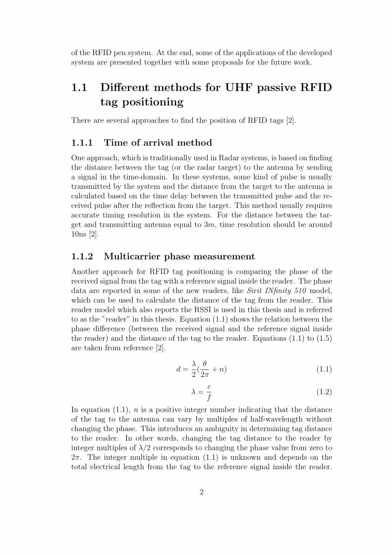
The method used in this thesis for tag positioning is based on the phase dif-ference between two antenna elements. This method leads to precise valuesfor tag positioning as shown later. Equation (1.6) which is derived from equa-tion (1.1) shows the relation between phase difference between two antennas(∆θ) and the difference in the distance of the tag to the phase center of eachantenna (∆d). This relationship is shown in Figure 1.1.

∆d =λ

2.∆θ

2π(1.6)

The phase ambiguity in equation (1.1) is removed in equation (1.6) as longas it is certain that the tag is placed in the non-ambiguity phase region. Thisnon-ambiguity phase region is derived for the geometry of the array in the nextsections. It is also shown how to use the hyperbolic functions, ∆d = const.,to find the tag position.

It is important to emphasize here that equations (1.1) to (1.6) are fora mono-static system in which one port is used for both transmission and

3

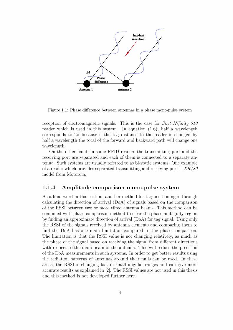
Figure 1.1: Phase difference between antennas in a phase mono-pulse system

reception of electromagnetic signals. This is the case for Sirit INfinity 510reader which is used in this system. In equation (1.6), half a wavelengthcorresponds to 2π because if the tag distance to the reader is changed byhalf a wavelength the total of the forward and backward path will change onewavelength.

On the other hand, in some RFID readers the transmitting port and thereceiving port are separated and each of them is connected to a separate an-tenna. Such systems are usually referred to as bi-static systems. One exampleof a reader which provides separated transmitting and receiving port is XR480model from Motorola.

1.1.4 Amplitude comparison mono-pulse system

As a final word in this section, another method for tag positioning is throughcalculating the direction of arrival (DoA) of signals based on the comparisonof the RSSI between two or more tilted antenna beams. This method can becombined with phase comparison method to clear the phase ambiguity regionby finding an approximate direction of arrival (DoA) for tag signal. Using onlythe RSSI of the signals received by antenna elements and comparing them tofind the DoA has one main limitation compared to the phase comparison.The limitation is that the RSSI value is not changing relatively, as much asthe phase of the signal based on receiving the signal from different directionswith respect to the main beam of the antenna. This will reduce the precisionof the DoA measurements in such systems. In order to get better results usingthe radiation patterns of antennas around their nulls can be used. In theseareas, the RSSI is changing fast in small angular ranges and can give moreaccurate results as explained in [2]. The RSSI values are not used in this thesisand this method is not developed further here.

4

Chapter 2

Array configuration andantenna design

The antenna elements used in the array are microstrip-fed Yagi-Uda antennas.Design procedure for the antenna is similar to what is explained in [4].

2.1 Radiation characteristics of the antenna

elements in the array

The simulation of the antenna with the method explained in [4] gives thedirectivity equal to 5dBi, front to back lobe ratio equal to 10dB and 3dBbeam-width in the E-plane equal to 70 degrees at 900MHz. The antennais linearly polarized with the electric field parallel to the feed dipole and thedirector. The direction of the main beam of the antenna is from dipole towardthe director. The phase center of the antenna is located in the center of thefeed dipole.

2.2 Fabrication of the Microstrip-fed Yagi

antenna element

Figure 2.1 shows the antenna which consists of a microstrip feed line connectedto a ”J” shaped balun [5], a feed dipole and one director. The Microstrip-fedYagi antenna shown in Figure 2.1 is working at a frequency range around900MHz which covers the standard UHF RFID frequency range. The shortline near the 1cm label in the figure shows the scaling factor of the figure. Itshould be noted that the ”J” shaped balun in Figure 2.1 is placed on one sideof the substrate and the ground plane and the feed dipole which is made byextending the ground plane and the director are placed on the other side ofthe substrate. In Figure 2.1 the observer is looking through the substrate.

Figure 2.2 shows the dimensions of the designed antenna. In this figure,L1 = 12.8cm, L2 = 6.1cm, L3 = 10cm, L4 = 5.5cm, L5 = 3.2cm and L6 =

5

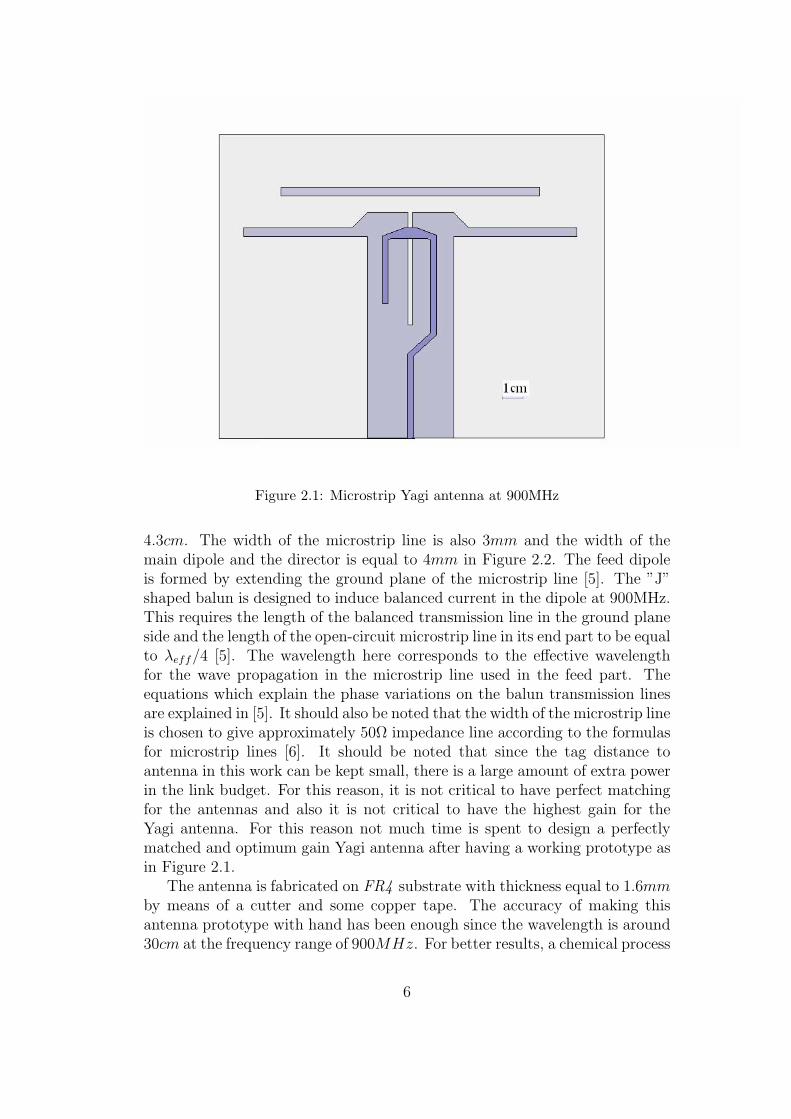
Figure 2.1: Microstrip Yagi antenna at 900MHz

4.3cm. The width of the microstrip line is also 3mm and the width of themain dipole and the director is equal to 4mm in Figure 2.2. The feed dipoleis formed by extending the ground plane of the microstrip line [5]. The ”J”shaped balun is designed to induce balanced current in the dipole at 900MHz.This requires the length of the balanced transmission line in the ground planeside and the length of the open-circuit microstrip line in its end part to be equalto λeff/4 [5]. The wavelength here corresponds to the effective wavelengthfor the wave propagation in the microstrip line used in the feed part. Theequations which explain the phase variations on the balun transmission linesare explained in [5]. It should also be noted that the width of the microstrip lineis chosen to give approximately 50Ω impedance line according to the formulasfor microstrip lines [6]. It should be noted that since the tag distance toantenna in this work can be kept small, there is a large amount of extra powerin the link budget. For this reason, it is not critical to have perfect matchingfor the antennas and also it is not critical to have the highest gain for theYagi antenna. For this reason not much time is spent to design a perfectlymatched and optimum gain Yagi antenna after having a working prototype asin Figure 2.1.

The antenna is fabricated on FR4 substrate with thickness equal to 1.6mmby means of a cutter and some copper tape. The accuracy of making thisantenna prototype with hand has been enough since the wavelength is around30cm at the frequency range of 900MHz. For better results, a chemical process

6

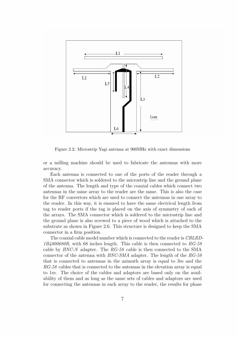
Figure 2.2: Microstrip Yagi antenna at 900MHz with exact dimensions

or a milling machine should be used to fabricate the antennas with moreaccuracy.

Each antenna is connected to one of the ports of the reader through aSMA connector which is soldered to the microstrip line and the ground planeof the antenna. The length and type of the coaxial cables which connect twoantennas in the same array to the reader are the same. This is also the casefor the RF convertors which are used to connect the antennas in one array tothe reader. In this way, it is ensured to have the same electrical length fromtag to reader ports if the tag is placed on the axis of symmetry of each ofthe arrays. The SMA connector which is soldered to the microstrip line andthe ground plane is also screwed to a piece of wood which is attached to thesubstrate as shown in Figure 2.6. This structure is designed to keep the SMAconnector in a firm position.

The coaxial cable model number which is connected to the reader is CBLRD-1B4000680R, with 68 inches length. This cable is then connected to RG-58cable by BNC-N adapter. The RG-58 cable is then connected to the SMAconnector of the antenna with BNC-SMA adapter. The length of the RG-58that is connected to antennas in the azimuth array is equal to 3m and theRG-58 cables that is connected to the antennas in the elevation array is equalto 1m. The choice of the cables and adaptors are based only on the avail-ability of them and as long as the same sets of cables and adaptors are usedfor connecting the antennas in each array to the reader, the results for phase

7

difference in each array remains unchanged.

2.3 Azimuth and elevation one-dimensional

arrays

In the fabricated arrays for azimuth and elevation, two of the Yagi antennas inFigure 2.1 are placed beside each other as shown in Figure 2.3. The distancebetween the phase centers of two antennas is equal to 24.3cm. This specialdistance has been the minimum possible distance between antennas due tothe mechanical constraints in fabricating the array mount with the woodenstructure. The distance is kept minimum to increase the phase clarity regionas will be explained later. Since the dipole elements in two antennas are placedalong each other where they have a null in their radiation pattern, the mutualimpedance between two antennas will become small. This is an importantissue in phase measurement as the phase should only be related to the pathlength from tag to the antenna and should not be affected from the inducedcurrent on the other antennas in the array.

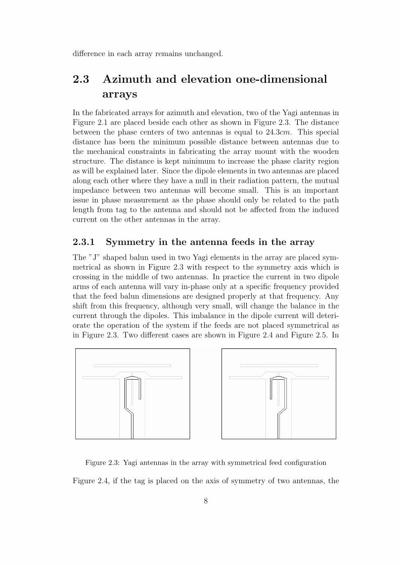
2.3.1 Symmetry in the antenna feeds in the array

The ”J” shaped balun used in two Yagi elements in the array are placed sym-metrical as shown in Figure 2.3 with respect to the symmetry axis which iscrossing in the middle of two antennas. In practice the current in two dipolearms of each antenna will vary in-phase only at a specific frequency providedthat the feed balun dimensions are designed properly at that frequency. Anyshift from this frequency, although very small, will change the balance in thecurrent through the dipoles. This imbalance in the dipole current will deteri-orate the operation of the system if the feeds are not placed symmetrical asin Figure 2.3. Two different cases are shown in Figure 2.4 and Figure 2.5. In

Figure 2.3: Yagi antennas in the array with symmetrical feed configuration

Figure 2.4, if the tag is placed on the axis of symmetry of two antennas, the

8

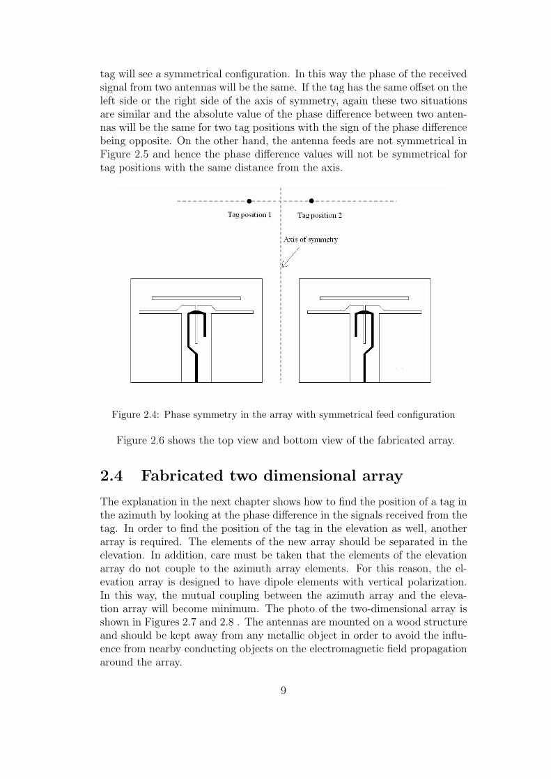
tag will see a symmetrical configuration. In this way the phase of the receivedsignal from two antennas will be the same. If the tag has the same offset on theleft side or the right side of the axis of symmetry, again these two situationsare similar and the absolute value of the phase difference between two anten-nas will be the same for two tag positions with the sign of the phase differencebeing opposite. On the other hand, the antenna feeds are not symmetrical inFigure 2.5 and hence the phase difference values will not be symmetrical fortag positions with the same distance from the axis.

Figure 2.4: Phase symmetry in the array with symmetrical feed configuration

Figure 2.6 shows the top view and bottom view of the fabricated array.

2.4 Fabricated two dimensional array

The explanation in the next chapter shows how to find the position of a tag inthe azimuth by looking at the phase difference in the signals received from thetag. In order to find the position of the tag in the elevation as well, anotherarray is required. The elements of the new array should be separated in theelevation. In addition, care must be taken that the elements of the elevationarray do not couple to the azimuth array elements. For this reason, the el-evation array is designed to have dipole elements with vertical polarization.In this way, the mutual coupling between the azimuth array and the eleva-tion array will become minimum. The photo of the two-dimensional array isshown in Figures 2.7 and 2.8 . The antennas are mounted on a wood structureand should be kept away from any metallic object in order to avoid the influ-ence from nearby conducting objects on the electromagnetic field propagationaround the array.

9

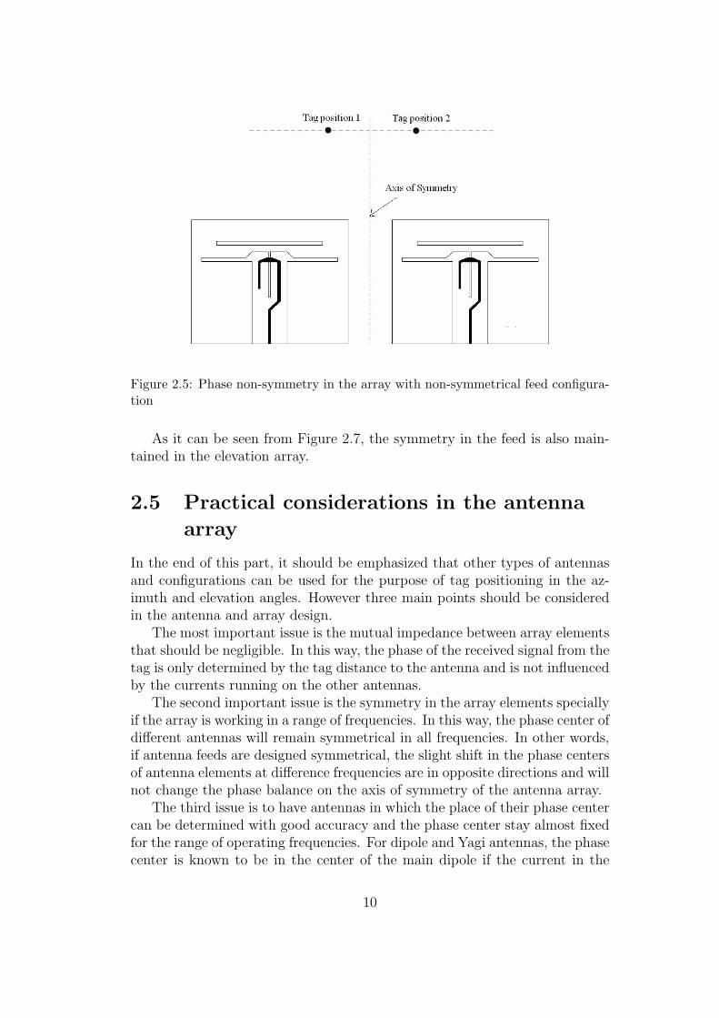
Figure 2.5: Phase non-symmetry in the array with non-symmetrical feed configura-tion

As it can be seen from Figure 2.7, the symmetry in the feed is also main-tained in the elevation array.

2.5 Practical considerations in the antenna

array

In the end of this part, it should be emphasized that other types of antennasand configurations can be used for the purpose of tag positioning in the az-imuth and elevation angles. However three main points should be consideredin the antenna and array design.

The most important issue is the mutual impedance between array elementsthat should be negligible. In this way, the phase of the received signal from thetag is only determined by the tag distance to the antenna and is not influencedby the currents running on the other antennas.

The second important issue is the symmetry in the array elements speciallyif the array is working in a range of frequencies. In this way, the phase center ofdifferent antennas will remain symmetrical in all frequencies. In other words,if antenna feeds are designed symmetrical, the slight shift in the phase centersof antenna elements at difference frequencies are in opposite directions and willnot change the phase balance on the axis of symmetry of the antenna array.

The third issue is to have antennas in which the place of their phase centercan be determined with good accuracy and the phase center stay almost fixedfor the range of operating frequencies. For dipole and Yagi antennas, the phasecenter is known to be in the center of the main dipole if the current in the

10

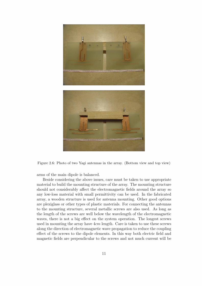
Figure 2.6: Photo of two Yagi antennas in the array. (Bottom view and top view)

arms of the main dipole is balanced.Beside considering the above issues, care must be taken to use appropriate

material to build the mounting structure of the array. The mounting structureshould not considerably affect the electromagnetic fields around the array soany low-loss material with small permittivity can be used. In the fabricatedarray, a wooden structure is used for antenna mounting. Other good optionsare plexiglass or other types of plastic materials. For connecting the antennasto the mounting structure, several metallic screws are also used. As long asthe length of the screws are well below the wavelength of the electromagneticwaves, there is not a big effect on the system operation. The longest screwsused in mounting the array have 4cm length. Care is taken to use these screwsalong the direction of electromagnetic wave propagation to reduce the couplingeffect of the screws to the dipole elements. In this way both electric field andmagnetic fields are perpendicular to the screws and not much current will be

11

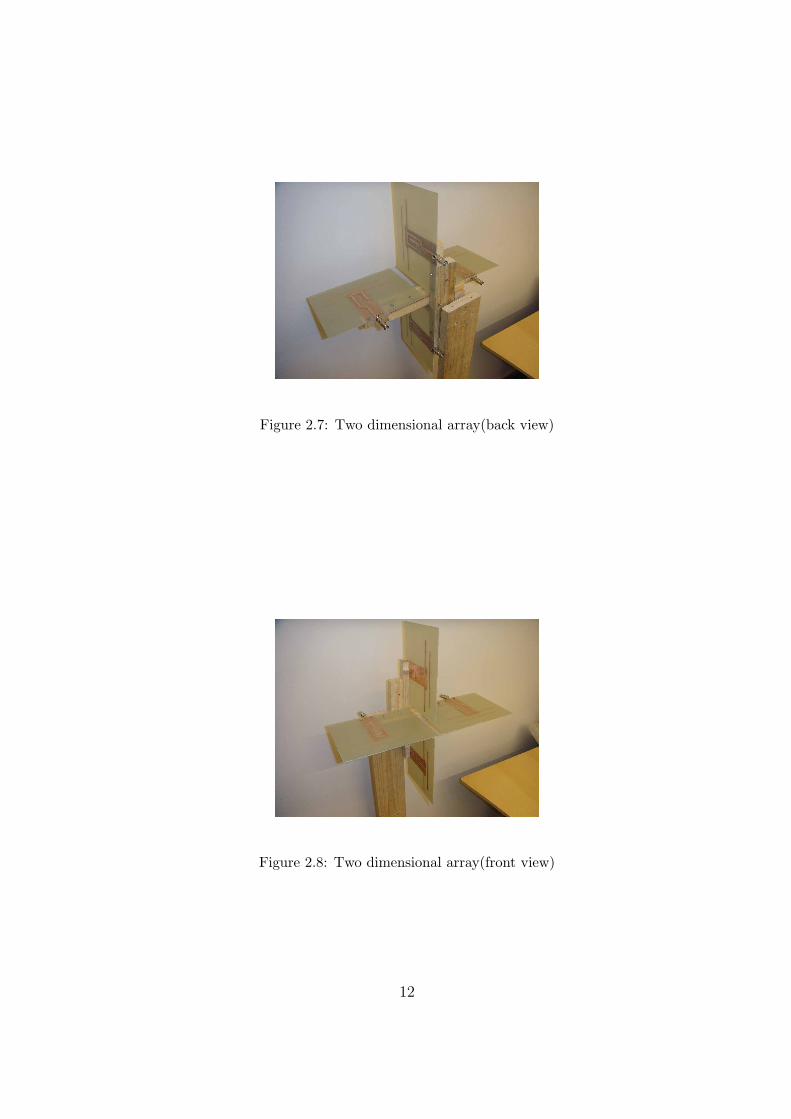
Figure 2.7: Two dimensional array(back view)

Figure 2.8: Two dimensional array(front view)

12

induced on them.

13

Chapter 3

Studying the measurementresults, how to get from phasedata to the actual location

In this part, the geometry of the array explained in the last part is studied inorder to get the actual position of the tag from measurement results for thephase difference between array elements. The measurement results are thencompared with the theory for validation. The phase measurements are doneat the frequency F = 869.525MHz. The RFID reader model which is used inthis thesis is Sirit INfinity 510 and the tag model number is AD-223.

3.1 Geometry of the array

Figure 3.1 shows the measurement setup and tag placement for the results inthis part. A cardboard is placed in front of the array with a tag attached to itsback as shown in Figure 3.1. In the measurements in this part, two antennasin the azimuth array are connected to port one and port two of the reader.The tag is attached to one side of the cardboard with some paper tapes with45 degrees slope with respect to the horizontal line as is shown in Figure 3.3.

Considering the tag facing to the antenna array, the antenna on the rightside of the tag is named antenna one and is connected to port one of the reader.The antenna on the left side of the tag is named antenna two and is connectedto the port two of the reader. The upper antenna in the elevation array isnamed antenna three and is connected to port three of the reader. The lowerantenna in the elevation array is named antenna four and is connected to portfour of the reader. The cable length and RF convertors used in connectingantenna one and antenna two to the reader are the same as given before. Thisis also the case for the cables and convertors connecting antenna three andantenna four to the reader.

The coordinate system used in studying the system is shown in Figure 3.2.The tag is placed on the other side of the cardboard and can not be seen in

14

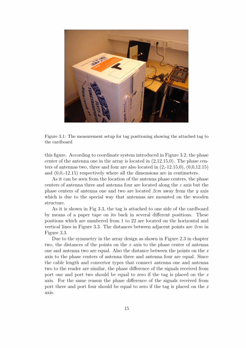
Figure 3.1: The measurement setup for tag positioning showing the attached tag tothe cardboard

this figure. According to coordinate system introduced in Figure 3.2, the phasecenter of the antenna one in the array is located in (2,12.15,0). The phase cen-ters of antennas two, three and four are also located in (2,-12.15,0), (0,0,12.15)and (0,0,-12.15) respectively where all the dimensions are in centimeters.

As it can be seen from the location of the antenna phase centers, the phasecenters of antenna three and antenna four are located along the z axis but thephase centers of antenna one and two are located 2cm away from the y axiswhich is due to the special way that antennas are mounted on the woodenstructure.

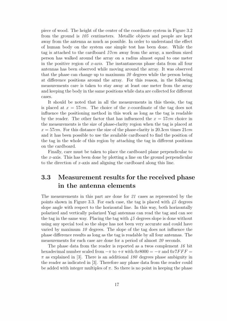
As it is shown in Fig 3.3, the tag is attached to one side of the cardboardby means of a paper tape on its back in several different positions. Thesepositions which are numbered from 1 to 22 are located on the horizontal andvertical lines in Figure 3.3. The distances between adjacent points are 2cm inFigure 3.3.

Due to the symmetry in the array design as shown in Figure 2.3 in chaptertwo, the distances of the points on the x axis to the phase center of antennaone and antenna two are equal. Also the distance between the points on the xaxis to the phase centers of antenna three and antenna four are equal. Sincethe cable length and convertor types that connect antenna one and antennatwo to the reader are similar, the phase difference of the signals received fromport one and port two should be equal to zero if the tag is placed on the xaxis. For the same reason the phase difference of the signals received fromport three and port four should be equal to zero if the tag is placed on the xaxis.

15

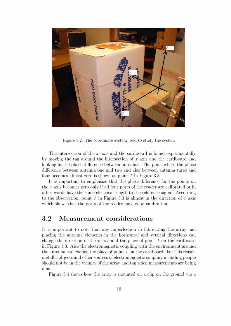
Figure 3.2: The coordinate system used to study the system

The intersection of the x axis and the cardboard is found experimentallyby moving the tag around the intersection of x axis and the cardboard andlooking at the phase difference between antennas. The point where the phasedifference between antenna one and two and also between antenna three andfour becomes almost zero is shown as point 1 in Figure 3.3.

It is important to emphasize that the phase difference for the points onthe x axis becomes zero only if all four ports of the reader are calibrated or inother words have the same electrical length to the reference signal. Accordingto the observation, point 1 in Figure 3.3 is almost in the direction of x axiswhich shows that the ports of the reader have good calibration.

3.2 Measurement considerations

It is important to note that any imperfection in fabricating the array andplacing the antenna elements in the horizontal and vertical directions canchange the direction of the x axis and the place of point 1 on the cardboardin Figure 3.3. Also the electromagnetic coupling with the environment aroundthe antenna can change the place of point 1 on the cardboard. For this reasonmetallic objects and other sources of electromagnetic coupling including peopleshould not be in the vicinity of the array and tag when measurements are beingdone.

Figure 3.4 shows how the array is mounted on a clip on the ground via a

16

piece of wood. The height of the center of the coordinate system in Figure 3.2from the ground is 105 centimeters. Metallic objects and people are keptaway from the antenna as much as possible. In order to understand the effectof human body on the system one simple test has been done. While thetag is attached to the cardboard 57cm away from the array, a medium sizedperson has walked around the array on a radius almost equal to one meterin the positive region of x-axis. The instantaneous phase data from all fourantennas has been observed while moving around the array. It was observedthat the phase can change up to maximum 20 degrees while the person beingat difference positions around the array. For this reason, in the followingmeasurements care is taken to stay away at least one meter from the arrayand keeping the body in the same positions while data are collected for differentcases.

It should be noted that in all the measurements in this thesis, the tagis placed at x = 57cm. The choice of the x -coordinate of the tag does notinfluence the positioning method in this work as long as the tag is readableby the reader. The other factor that has influenced the x = 57cm choice inthe measurements is the size of phase-clarity region when the tag is placed atx = 57cm. For this distance the size of the phase-clarity is 20.3cm times 21cmand it has been possible to use the available cardboard to find the position ofthe tag in the whole of this region by attaching the tag in different positionson the cardboard.

Finally, care must be taken to place the cardboard plane perpendicular tothe x -axis. This has been done by plotting a line on the ground perpendicularto the direction of x -axis and aligning the cardboard along this line.

3.3 Measurement results for the received phase

in the antenna elements

The measurements in this part are done for 21 cases as represented by thepoints shown in Figure 3.3. For each case, the tag is placed with 45 degreesslope angle with respect to the horizontal line. In this way, both horizontallypolarized and vertically polarized Yagi antennas can read the tag and can seethe tag in the same way. Placing the tag with 45 degrees slope is done withoutusing any special tool so the slope has not been very accurate and could havevaried by maximum 10 degrees. The slope of the tag does not influence thephase difference results as long as the tag is readable by all four antennas. Themeasurements for each case are done for a period of almost 20 seconds.

The phase data from the reader is reported as a twos complement 16 bithexadecimal number scaled from −π to +π with 0x8000 = −π and 0x7FFF =π as explained in [3]. There is an additional 180 degrees phase ambiguity inthe reader as indicated in [3]. Therefore any phase data from the reader couldbe added with integer multiples of π. So there is no point in keeping the phase

17

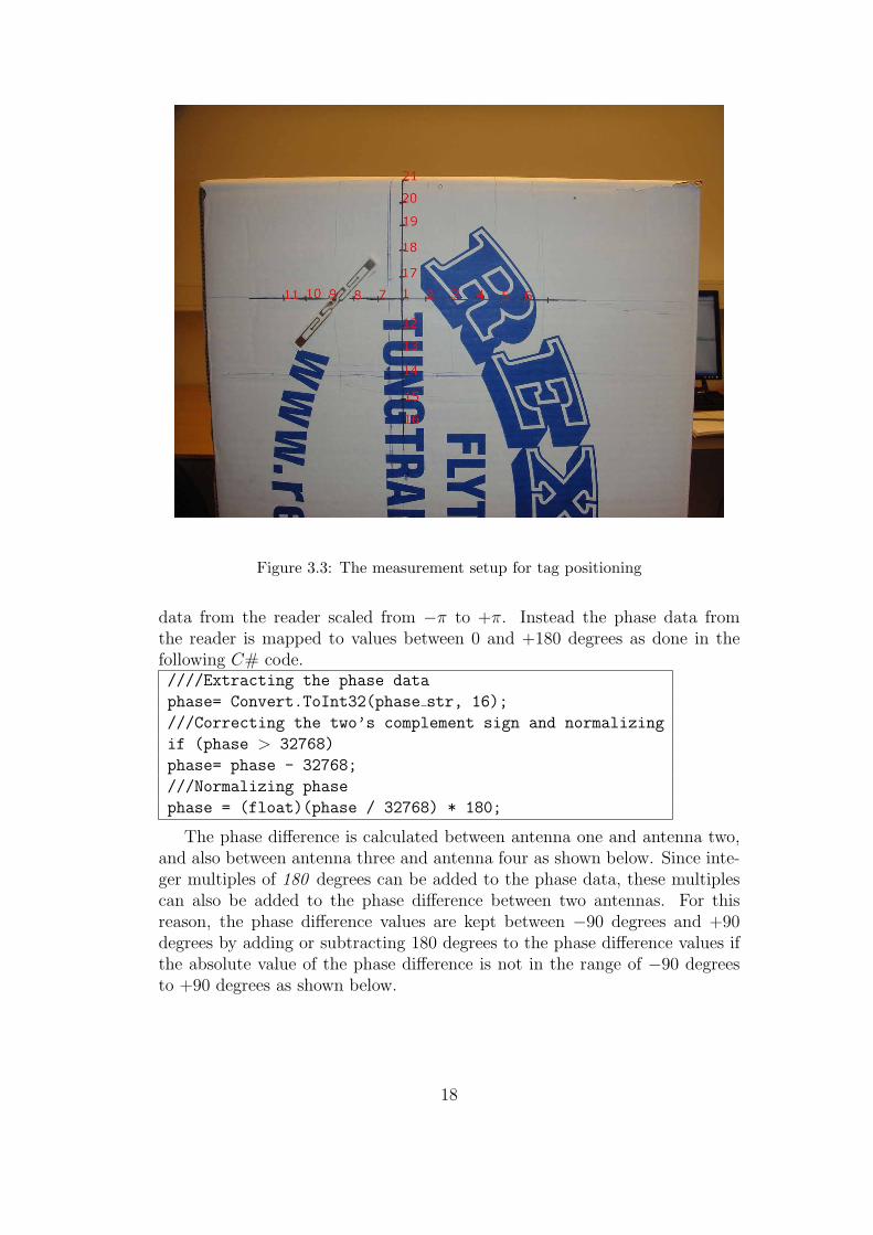
Figure 3.3: The measurement setup for tag positioning

data from the reader scaled from −π to +π. Instead the phase data fromthe reader is mapped to values between 0 and +180 degrees as done in thefollowing C# code.////Extracting the phase data

phase= Convert.ToInt32(phase str, 16);

///Correcting the two’s complement sign and normalizing

if (phase > 32768)

phase= phase - 32768;

///Normalizing phase

phase = (float)(phase / 32768) * 180;

The phase difference is calculated between antenna one and antenna two,and also between antenna three and antenna four as shown below. Since inte-ger multiples of 180 degrees can be added to the phase data, these multiplescan also be added to the phase difference between two antennas. For thisreason, the phase difference values are kept between −90 degrees and +90degrees by adding or subtracting 180 degrees to the phase difference values ifthe absolute value of the phase difference is not in the range of −90 degreesto +90 degrees as shown below.

18

Figure 3.4: Mounting the array on a holder

//Calculating phase difference

phasediff12 = phase2- phase1;

phasediff34 = phase3- phase4;

//Scaling the phase difference between -90 and +90

if (Math.Abs(phasediff12 > 90))

phasediff12=phasediff12-180*Math.Sign(phasediff12);

if (Math.Abs(phasediff34 > 90))

phasediff34=phasediff34-180*Math.Sign(phasediff34);

The results of the measurements are shown in Table 3.1 and Table 3.2.The phase data are reported in degrees and the RSSI values are reportedin ddBm(deci dBm). The data in Table 3.1 and Table 3.2 are the averagevalues over the measurements in each case. The data for Phase1, Phase2 andPhasediff12 are calculated as explained in the above codes. The last columnshows the number of data points that is used for averaging to get the phasedifference data in each case.

The data in Table 3.1 are for study cases 1 to 11 as represented by thepoints shown in Figure 3.3. As it can be seen in Figure 3.3, for the cases 1to 11, the tag is moved on the horizontal axis or in the azimuth direction.The upper part of Table 3.1 shows the phase data from antenna one and

19

antenna two. As it can be seen, the phase difference between antenna oneand two is varying in the upper part of the table based on the tag positionon the horizontal axis. On the other hand, in the bottom part of the table,the phase data from antenna three and four are given which shows the phasedifference between antenna three and four stays around zero with maximum21.0263 degrees variation. This is expected since the path length from tag tothe phase center of antenna three and antenna four remains the same whilemoving the tag on the horizontal line.

The data in Table 3.2 are for the study cases 12 to 21 in which the tag ismoved on the vertical axis as shown in Figure 3.3. In Table 3.2, the upper partgives the phase data from antenna three and four which shows the variation ofphase difference between antenna three and antenna four based on the positionof the tag on the vertical axis. On the other hand, the bottom part in Table 3.2shows that the phase difference between antenna one and two remains aroundzero with maximum 20.4655 degrees variation. The reason is that the pathlength from the tag to the phase centers of antenna one and two remainsunchanged here while moving the tag on the vertical axis.

It is also important to state that the antenna beamwidth and directionalityhas not any effect on the phase values. Antenna directionality and beamwidthchanges the values of RSSI based on the position of the tag which is not studiedin this thesis. However, in Table 3.1 and Table 3.2, the values of the measuredRSSI are also given for each case so the reader has some idea about the rangeof the values.

3.4 Finding the position of the tag in the az-

imuth plane

Using the phase difference in Table 3.1, the position of tag can be calculatedfrom equation (3.1) where d1 and d2 are the distance of the tag to the phasecenters of antennas one and two. The phase of the received signal from antennaone and two is shown by θ1 and θ2. The phase center of the antenna one islocated in (a,b,0)=(2,12.15,0) and the phase center of antenna two is locatedat (a,-b,0)=(2,-12.15,0).

Since in the measurement in Table 3.1 the tag is located in the azimuthplane, or placed in the xy plane as shown in Figure 3.2, the distance of tag toantenna three and four remains constant. So the data should show ∆θ34 ≈ 0as can be seen from the second part of Table 3.1. For the tag distance to thephase centers of antenna one and two:

∆d21 = d2 − d1 =λ

2.∆θ212π

(3.1)

d2 =√(x− a)2 + (y + b)2 (3.2)

d1 =√

(x− a)2 + (y − b)2 (3.3)

20

Case Phase1 Phase2 Phasediff12 RSSI1 RSSI2 Data No.11 146.9753 45.6709 78.6300 -583.2430 -565.9129 165510 129.1889 45.1021 -83.9239 -571.6596 -568.9729 18849 116.1819 54.5808 -61.5432 -564.4327 -570.8389 15058 101.2098 62.8099 -38.3518 -562.8316 -589.3338 18797 91.6251 70.9694 -20.4327 -555.8514 -592.1325 11301 91.8678 89.3033 -2.5081 -536.1991 -584.9370 11142 88.7042 99.5106 10.8995 -528.7101 -587.7921 12443 78.6248 113.9923 35.5162 -530.6091 -605.0395 12404 75.4080 125.5567 50.1416 -529.5556 -619.6325 12445 75.2601 146.0122 70.7566 -525.9114 -629.0615 12436 79.4728 72.8249 -79.3681 -521.9817 -637.8873 1504

Case Phase3 Phase4 Phasediff34 RSSI3 RSSI4 Data No.11 9.3287 171.8671 15.1266 -485.0527 -516.8946 165410 170.9252 155.5424 15.3077 -493.7277 -532.5586 20659 170.2756 149.3746 21.0263 -500.2804 -530.0578 16448 161.3149 146.6076 14.7154 -493.8572 -515.4363 16527 144.9448 141.0185 3.9322 -509.1523 -523.2540 12411 141.6534 142.2750 -0.6451 -525.0044 -537.1069 10782 141.7179 148.0773 -6.5765 -530.8777 -533.7665 11253 141.9164 145.6325 -3.9952 -511.4802 -517.2086 15044 146.1787 148.7251 -3.6961 -502.8997 -511.3236 14985 148.8661 156.4788 -7.5856 -499.9898 -512.5937 15056 165.5385 168.3817 -2.6611 -496.7818 -508.1669 1487

Table 3.1: Average values for the phase measurement results by moving tag in theazimuth direction

Now using equations (3.2) and (3.3) in (3.1) gives√(x− a)2 + (y + b)2 −

√(x− a)2 + (y − b)2 = ∆d21 (3.4)

Which can be written as

x = ±√

(2by

∆d21− ∆d21

2)2 − (y − b)2 + a (3.5)

Since the tag is located in the positive part of x axis, the positive sign behindthe root square in (3.5) should be chosen. In theory, it is not possible to findout if the tag is located in the positive part or the negative part of the x -axisbased on the values of the phase difference between antennas. However inpractice due to the directionality of the antennas used in the array towardthe positive x -axis, only the tags which are placed in front of the array in thepositive x -axis direction can be read.

Now using the values in Table 3.1 for phasediff12 in (3.1), equation (3.5)is plotted for each case in Figure 3.5. According to equation (3.1), when

21

Case Phase3 Phase4 Phasediff34 RSSI3 RSSI4 Data No.21 140.8853 53.3294 85.0342 -493.4949 -574.8873 165920 144.7081 27.2950 -63.7564 -503.0229 -571.2524 225519 143.0855 16.5725 -54.1326 -516.6076 -564.7540 188218 142.8394 168.7603 -25.9639 -499.9788 -548.7108 150217 148.3863 150.8365 -2.4348 -520.7661 -538.5698 22281 141.6534 142.2750 -0.6451 -525.0044 -537.1069 107812 143.2832 129.1550 14.1203 -525.9868 -521.5381 166313 155.0148 116.3421 38.7616 -513.6508 -505.6413 166714 158.4788 104.6829 53.7964 -526.6537 -504.3982 166615 168.0533 98.4211 69.6346 -538.1274 -501.5146 165416 170.0022 90.1350 79.9668 -538.4085 -501.8748 1644

Case Phase1 Phase2 Phasediff12 RSSI1 RSSI2 Data No.21 101.6778 119.1811 17.4837 -551.0212 -630.9714 165920 101.1066 103.0028 1.7993 -530.4624 -605.6626 198519 98.7216 93.8427 -4.4465 -524.5161 -595.2533 188318 89.3472 82.9210 -6.3489 -534.8514 -603.4473 150817 96.6231 82.7794 -13.9521 -525.1133 -585.0337 22611 91.8678 89.3033 -2.5081 -536.1991 -584.9370 111412 93.5606 85.1495 -8.2647 -533.2233 -575.2621 150313 97.1449 88.8310 -8.3148 -540.8170 -580.3580 150314 104.3945 91.3440 -13.1405 -537.4619 -571.8023 150015 112.1464 99.0015 -13.2402 -527.0805 -559.2870 150616 120.8474 100.5205 -20.4655 -523.2182 -562.7357 1874

Table 3.2: Average values for the phase measurement results by moving tag in theelevation direction

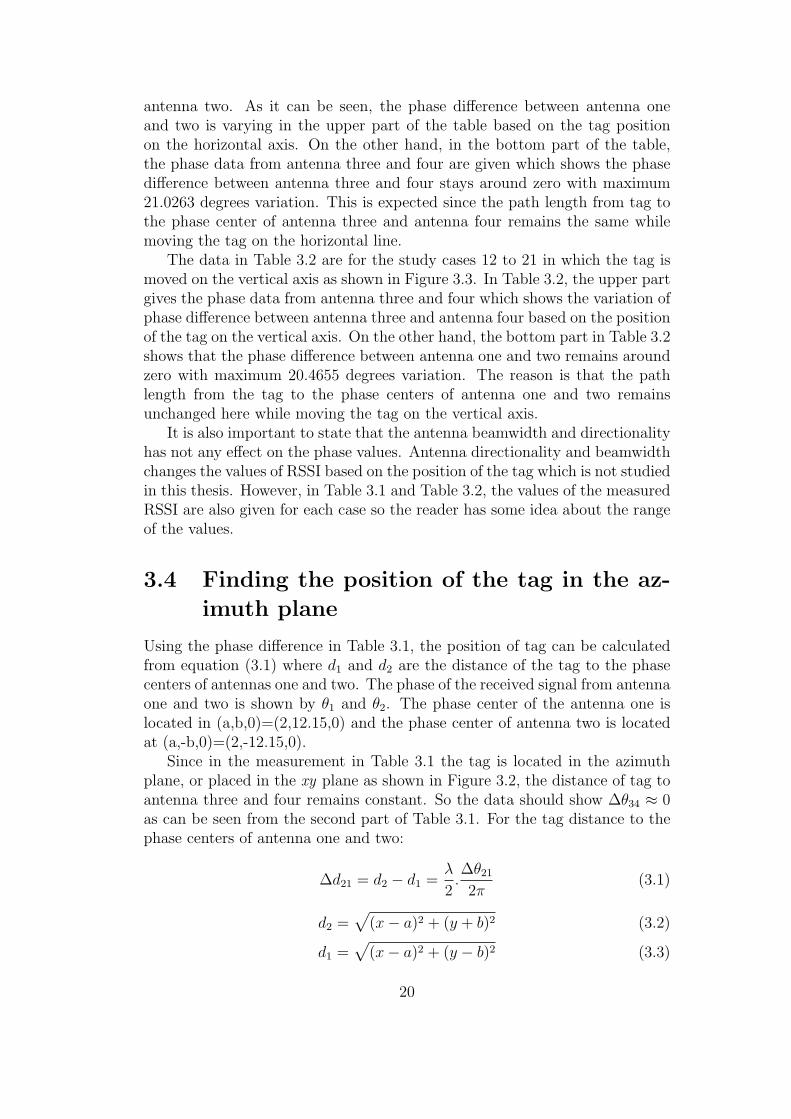
∆d21 > 0 the tag has to be in the positive part of y axis. For this reason,for each case in Figure 3.5, the positive or negative values for variable y arechosen to plot equation (3.5) based on the sign of ∆d21. Table 3.3 shows they coordinate of the position of the tag on the cardboard. The positions arederived from Figure 3.5 by finding the intersection of the hyperbolic functionin (3.5) for each case and the straight line of x=57cm. Phase ambiguity borderin Figure 3.5 is outside the hyperbolic functions on the border with thickerplot line. The intersection of these two functions with the straight line whichis representing the cardboard are located at y = ±10.15cm.

If the tag position is near the phase ambiguity border, there is a highprobability that the position of the tag be calculated in the wrong direction.This can be seen in case 11 and case 6 in Table 3.3.

22

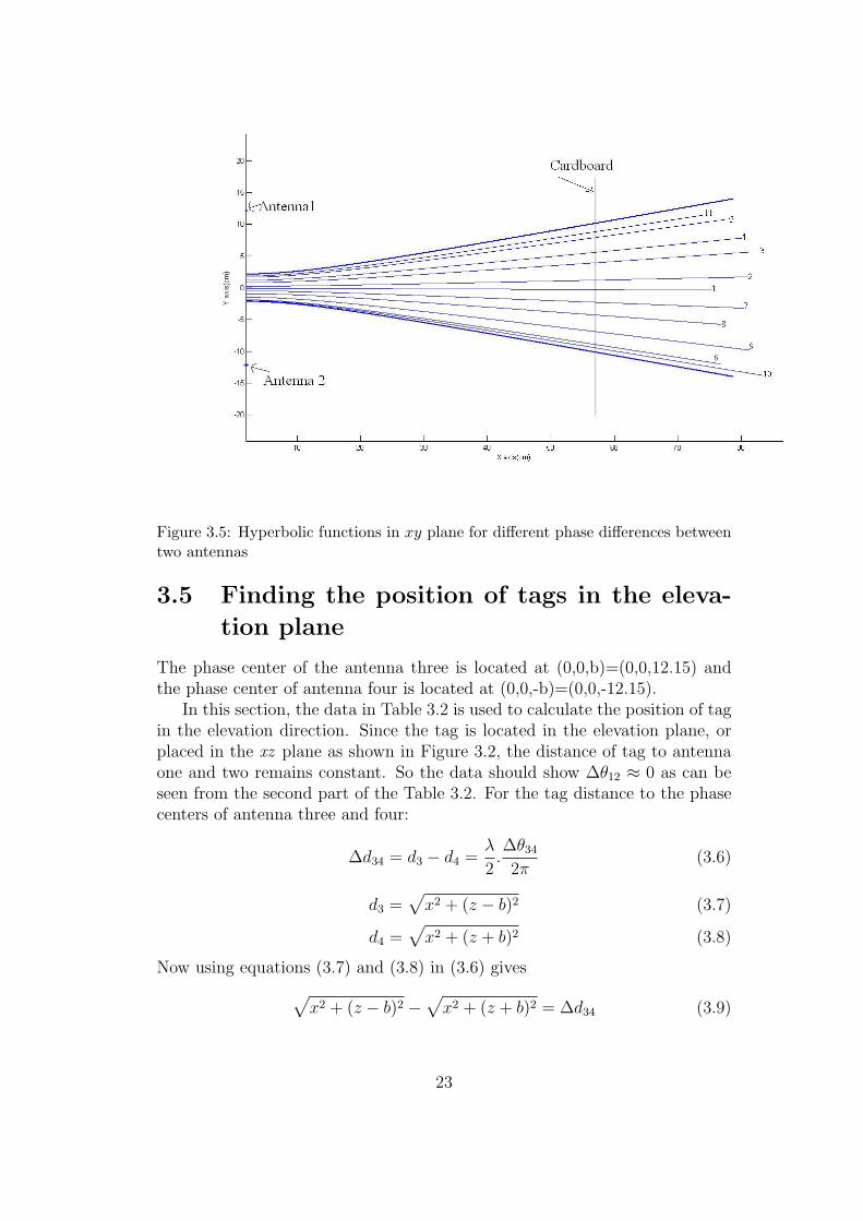
Figure 3.5: Hyperbolic functions in xy plane for different phase differences betweentwo antennas

3.5 Finding the position of tags in the eleva-

tion plane

The phase center of the antenna three is located at (0,0,b)=(0,0,12.15) andthe phase center of antenna four is located at (0,0,-b)=(0,0,-12.15).

In this section, the data in Table 3.2 is used to calculate the position of tagin the elevation direction. Since the tag is located in the elevation plane, orplaced in the xz plane as shown in Figure 3.2, the distance of tag to antennaone and two remains constant. So the data should show ∆θ12 ≈ 0 as can beseen from the second part of the Table 3.2. For the tag distance to the phasecenters of antenna three and four:

∆d34 = d3 − d4 =λ

2.∆θ342π

(3.6)

d3 =√

x2 + (z − b)2 (3.7)

d4 =√

x2 + (z + b)2 (3.8)

Now using equations (3.7) and (3.8) in (3.6) gives√x2 + (z − b)2 −

√x2 + (z + b)2 = ∆d34 (3.9)

23

Case study Phasediff12 Actual position(cm) Calculated position(cm)11 78.6300 -10 8.8310 -83.9239 -8 -9.449 -61.5432 -6 -6.888 -38.3518 -4 -4.277 -20.4327 -2 -2.271 -2.5081 0 -0.282 10.8995 2 1.213 35.5162 4 3.954 50.1416 6 5.595 70.7566 8 7.936 -79.3681 10 -8.92

Table 3.3: Calculated y coordinate tag position versus actual position in the xyplane

Which can be written as

x = ±√(−2bz

∆d34− ∆d34

2)2 − (z + b)2 (3.10)

Since the tag is located in the positive part of x axis, the positive sign behindthe root square in (3.10) is chosen.

Now using the values in Table 3.2 for phasediff34 in (3.6), equation (3.10)is plotted for each case in Figure 3.6. According to equation (3.6) , when∆d34 > 0 the tag has to be in the negative part of z axis. For this reasonfor each case in Figure 3.6, the positive or negative values for variable z arechosen to plot equation (3.10) based on the sign of ∆d34. Table 3.4 shows thez coordinate of the position of the tag on the cardboard. The positions arederived from Figure 3.6 by finding the intersection of the hyperbolic functionin (3.10) for each case and the straight line of x=57cm in the elevation plane.The phase ambiguity region is derived to be z = ±10.5cm.

Again, it can be seen that if the tag position is near the phase ambiguityborder, there is a high probability that the position of the tag be calculatedin the wrong direction. This can be seen in case 21 in Table 3.4.

3.6 Finding tag position in both elevation and

azimuth planes

For finding the tag position in both elevation and azimuth planes, equa-tions (3.1) and (3.6) should be solved simultaneously having in mind thatthe tag is placed on the cardboard or the plane with x = 57cm. The followingequations show the tag distance to the phase centers of antenna elements inthe array.

d1 =√(x− a)2 + (y − b)2 + z2 (3.11)

24

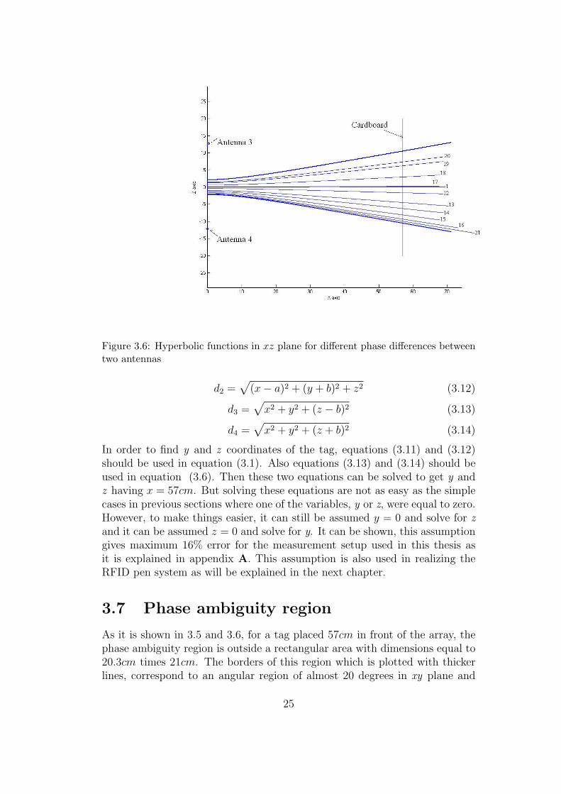
Figure 3.6: Hyperbolic functions in xz plane for different phase differences betweentwo antennas

d2 =√(x− a)2 + (y + b)2 + z2 (3.12)

d3 =√

x2 + y2 + (z − b)2 (3.13)

d4 =√x2 + y2 + (z + b)2 (3.14)

In order to find y and z coordinates of the tag, equations (3.11) and (3.12)should be used in equation (3.1). Also equations (3.13) and (3.14) should beused in equation (3.6). Then these two equations can be solved to get y andz having x = 57cm. But solving these equations are not as easy as the simplecases in previous sections where one of the variables, y or z, were equal to zero.However, to make things easier, it can still be assumed y = 0 and solve for zand it can be assumed z = 0 and solve for y. It can be shown, this assumptiongives maximum 16% error for the measurement setup used in this thesis asit is explained in appendix A. This assumption is also used in realizing theRFID pen system as will be explained in the next chapter.

3.7 Phase ambiguity region

As it is shown in 3.5 and 3.6, for a tag placed 57cm in front of the array, thephase ambiguity region is outside a rectangular area with dimensions equal to20.3cm times 21cm. The borders of this region which is plotted with thickerlines, correspond to an angular region of almost 20 degrees in xy plane and

25

Case study Phasediff34 Actual position(cm) Calculated position(cm)21 85.0342 10 -9.920 -63.7564 8 7.3819 -54.1326 6 6.2518 -25.9639 4 2.9917 -2.4348 2 0.281 -0.6451 0 0.0712 14.1203 -2 -1.6213 38.7616 -4 -4.4614 53.7964 -6 -6.2115 69.6346 -8 -8.0716 79.9668 -10 -9.3

Table 3.4: Calculated z coordinate of tag position versus actual position in the xzplane

xz plane as can be seen in Figure 3.5 and 3.6. Inside the region is the placewhere positioning can be done without ambiguity. This area is referred to asphase clarity area in this thesis.

For comparison, the phase clarity region for a phase mono-pulse systemis 180 degrees if the distance between the phase centers of two antennas ishalf a wavelength. There are three reasons for the smaller angular region withphase clarity in the measurements in this work, compared to the classic phasemono-pulse system.

The first reason is using the same antenna for transmitting and receivingelectromagnetic waves in our system. Also there is an additional 180 degreesphase ambiguity in the reader, as it is mentioned in [3], which will decreasethe region with phase clarity. Finally, the distance between antennas in thearray is equal to 24.3cm and is larger than λ/2(17.25cm) at the measurementfrequency(869.525MHz). Decreasing the distance between antennas to λ/2will increase the mutual impedance which will impair the system operation.The estimate on the amount of impairment of the system when decreasingantenna spacing should be based on a numerical analysis to get the mutualimpedance variation between antenna elements by varying the antenna spac-ing.

As a final word in this section, it should be noted that if the tag distanceto the array is increased, the phase clarity region will increase in a linear waywhile the hyperbolic functions as shown in Figure 3.5 and Figure 3.6 remainunchanged.

26

Chapter 4

Studying the resolution of thepositioning

The measurements in this work are done in an office environment. As discussedearlier, a simple test showed that if a person is moving around a circle, 1 meteraway from the array, the received phase from a tag attached almost 0.5 meteraway from the array can change up to 20 degrees. The reason for the change inthe phase of the received signal is that the presence of human body changes theelectromagnetic fields which are interacting between the tag and the antennaarray. However if the human body is not very close to the system, the changein the phase is small. For this reason, during the measurements, the metallicobjects and people are kept at least 1 meter away from the array. In thischapter the distribution of the phase data is studied first and after that atheoretical study is done for determining the resolution of positioning in themeasurements.

4.1 The variance of the phase difference data

Although the surrounding objects and people can shift the phase data from thetag, this shift in the phase will stay fixed as long as the environment aroundthe antenna does not change. For this reason, it is tried to keep the bodygesture of the experimenter fixed while measurements were going on for eachcase. This effect is specially important to study the variance of the phase datafor each case.

Figure 4.1 shows a sample distribution for the phase difference measure-ments between antenna three and antenna four which corresponds to case 15in Table 3.2. The number of data points in this distribution is 1654 which arecollected in the duration of around 30 seconds. If there were no movementsaround the antenna array, the distribution would be Gaussian. Any deviationfrom Gaussian distribution is attributed to large-scale changes in the environ-ment which has mainly been due to the changes in the body gesture of theexperimenter during the measurements. For this reason, it is not possible to

27

get a reliable value for the variance of the phase measurements data based onthe data that is collected. However, looking at several data sets at a fixed bodygesture the variance of the phase difference data is measured to be around one.This means that the standard deviation for the phase difference data is around1 degree which is an inherent characteristic of the RFID reader used in themeasurements.

One way to exclude the effect of the experimenter body on the phase datais to perform the test inside an anechoic chamber. In this way the experi-menter can stay outside the chamber and control the start and stop time ofthe measurement from outside the chamber.

Figure 4.1: A sample measured probability distribution function for phase differencedata

4.2 Probability of error for resolution of adja-

cent points

A theoretical study is performed in this section to find the resolution of posi-tioning, assuming the Gaussian distribution for the phase data.

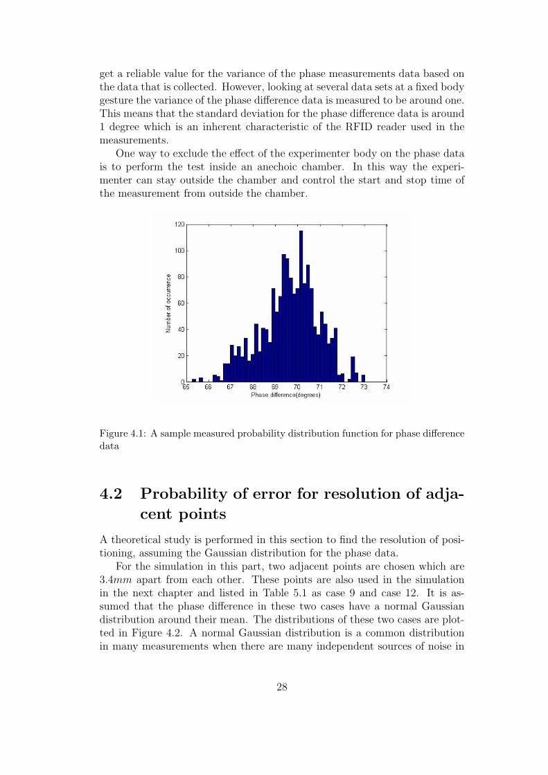
For the simulation in this part, two adjacent points are chosen which are3.4mm apart from each other. These points are also used in the simulationin the next chapter and listed in Table 5.1 as case 9 and case 12. It is as-sumed that the phase difference in these two cases have a normal Gaussiandistribution around their mean. The distributions of these two cases are plot-ted in Figure 4.2. A normal Gaussian distribution is a common distributionin many measurements when there are many independent sources of noise in

28

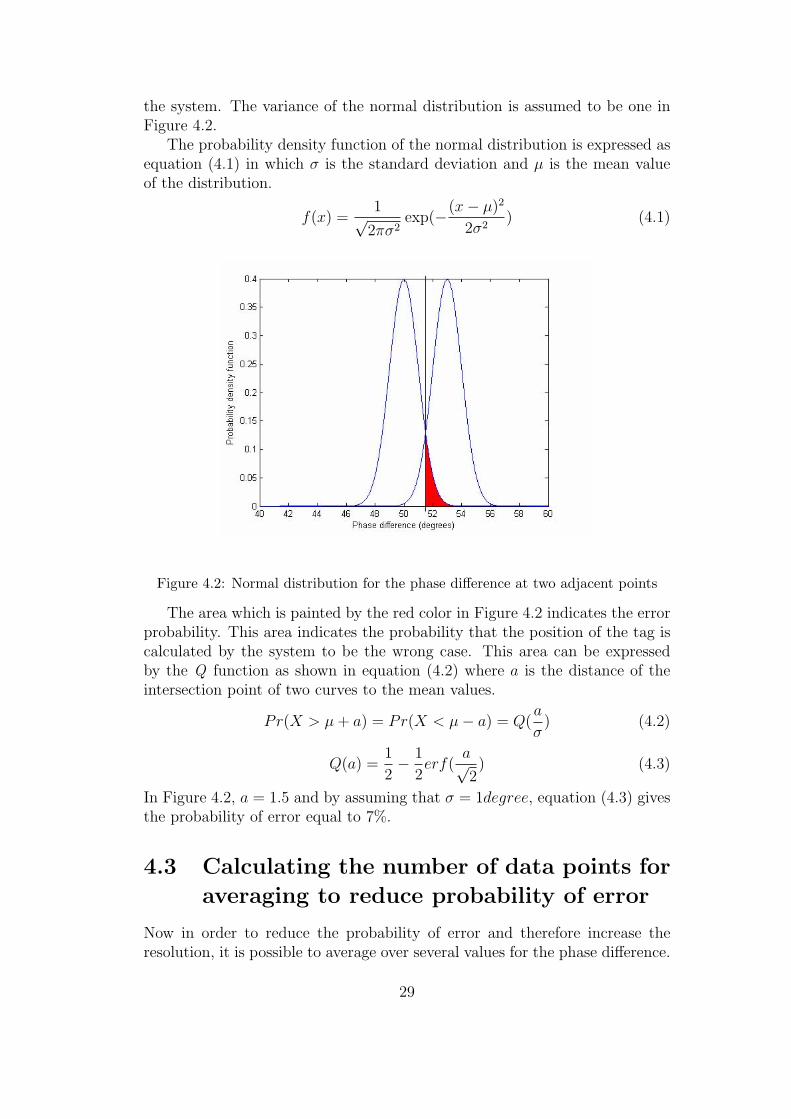
the system. The variance of the normal distribution is assumed to be one inFigure 4.2.

The probability density function of the normal distribution is expressed asequation (4.1) in which σ is the standard deviation and µ is the mean valueof the distribution.

f(x) =1√2πσ2

exp(−(x− µ)2

2σ2) (4.1)

Figure 4.2: Normal distribution for the phase difference at two adjacent points

The area which is painted by the red color in Figure 4.2 indicates the errorprobability. This area indicates the probability that the position of the tag iscalculated by the system to be the wrong case. This area can be expressedby the Q function as shown in equation (4.2) where a is the distance of theintersection point of two curves to the mean values.

Pr(X > µ+ a) = Pr(X < µ− a) = Q(a

σ) (4.2)

Q(a) =1

2− 1

2erf(

a√2) (4.3)

In Figure 4.2, a = 1.5 and by assuming that σ = 1degree, equation (4.3) givesthe probability of error equal to 7%.

4.3 Calculating the number of data points for

averaging to reduce probability of error

Now in order to reduce the probability of error and therefore increase theresolution, it is possible to average over several values for the phase difference.

29

According to the theory of normal random variables, if averaging is done over Nnormal distributed values with the standard deviation equal to σ, the result isagain a normal distributed random variable with the standard deviation givenby:

σaverage =σ√N

(4.4)

Now in order to have true resolution equal to 3 degrees between case 9 and12 (or 3.4mm as can be seen from Table 5.1) for 99% of the times, averagingshould be used over the data. The number of data points which are neededfor averaging can be calculated from equations (4.2) and (4.4).

According to these equations, the Q-table for 1% error probability givesN = 5.3 . So the number of data points for averaging should then be takenN = 6 as the first largest integer. So according to the calculations above,by averaging over 6 values for the phase difference between antenna one andantenna two, the position of the tag can be estimated correctly with the reso-lution of 3.4mm for 99% of the times.

30

Chapter 5

Specifications of the RFID pensystem and a sample result fordrawing

In this chapter, the specifications of a system which controls the mouse cursoron the computer screen by moving an RFID tag in the air is described. The tagis attached to a plastic rod, as shown in Figure 5.1, to keep the tag away fromthe body. This will decrease the coupling effect of the body on the phase ofthe signals received by the antenna array. Also it is recommended for the userto stay at least 1 meter away from the array while using the system. In thedeveloped system, the tag position in both azimuth and elevation directionsare calculated and mapped to the cursor position in real time. By using thesystem in practice, one can control the cursor easily and the precision of thecursor is enough to easily open or close windows and do all the usual tasksof a mouse. However the mouse click operation is not implemented in thesystem yet although some ideas are presented in the future work section toimplement this feature by detecting special tag movement. For demonstratingthe operation of the system, the first sentence that is written with the systemis shown in Figure 5.2. The file is created by moving the tag in the air andusing the Paint program in Windows. The mouse click is performed wheneverneeded with an ordinary mouse connected to the host computer.

As it was explained in previous chapters, moving the tag in front of thearray will change the phase difference in the signals received by four antennasin the array. This phase difference can then be used to find the location ofthe tag in both azimuth and elevation directions by solving some hyperbolicequations. However as it is explained in this section, it is possible to directlytransform the phase difference data to tag location with a linear transforationif the tag distance to the antenna array is not too small.

In the next section a theoretical study is done to show how the positionrelates to the linear increase in the phase difference between antennas.

31

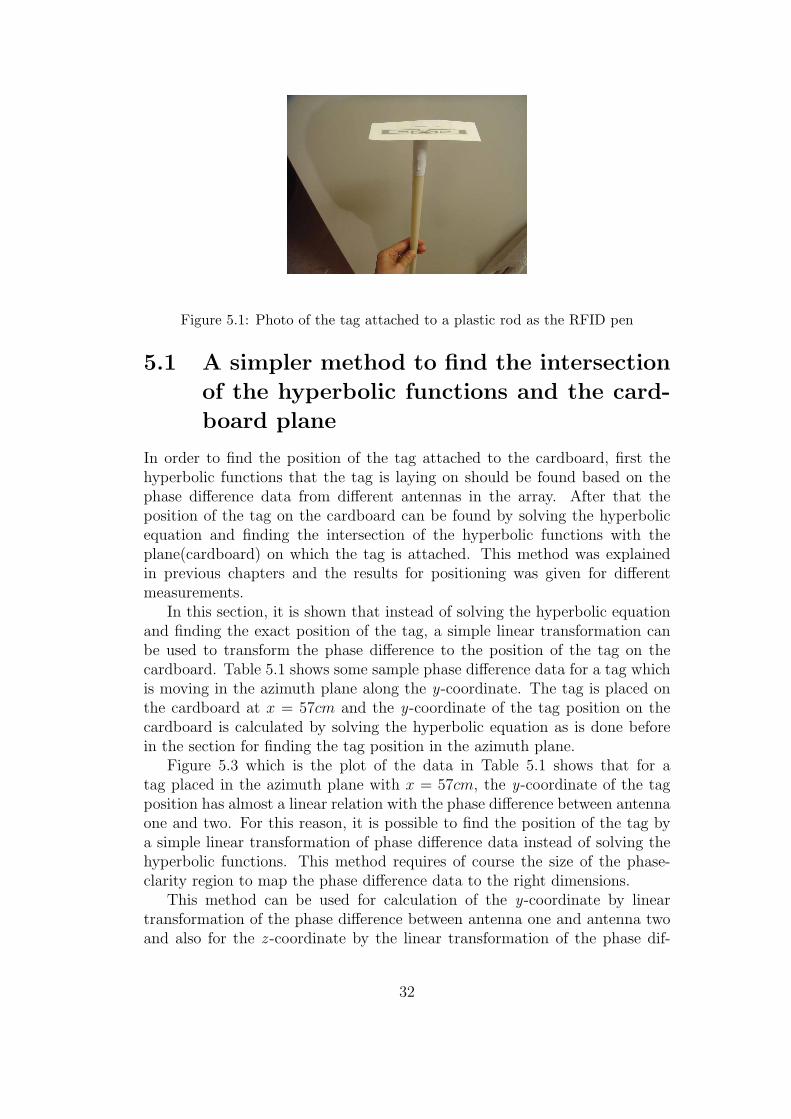
Figure 5.1: Photo of the tag attached to a plastic rod as the RFID pen

5.1 A simpler method to find the intersection

of the hyperbolic functions and the card-

board plane

In order to find the position of the tag attached to the cardboard, first thehyperbolic functions that the tag is laying on should be found based on thephase difference data from different antennas in the array. After that theposition of the tag on the cardboard can be found by solving the hyperbolicequation and finding the intersection of the hyperbolic functions with theplane(cardboard) on which the tag is attached. This method was explainedin previous chapters and the results for positioning was given for differentmeasurements.

In this section, it is shown that instead of solving the hyperbolic equationand finding the exact position of the tag, a simple linear transformation canbe used to transform the phase difference to the position of the tag on thecardboard. Table 5.1 shows some sample phase difference data for a tag whichis moving in the azimuth plane along the y-coordinate. The tag is placed onthe cardboard at x = 57cm and the y-coordinate of the tag position on thecardboard is calculated by solving the hyperbolic equation as is done beforein the section for finding the tag position in the azimuth plane.

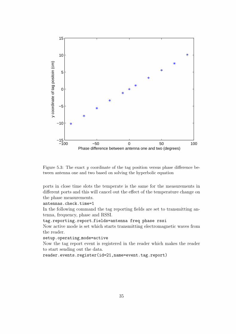
Figure 5.3 which is the plot of the data in Table 5.1 shows that for atag placed in the azimuth plane with x = 57cm, the y-coordinate of the tagposition has almost a linear relation with the phase difference between antennaone and two. For this reason, it is possible to find the position of the tag bya simple linear transformation of phase difference data instead of solving thehyperbolic functions. This method requires of course the size of the phase-clarity region to map the phase difference data to the right dimensions.

This method can be used for calculation of the y-coordinate by lineartransformation of the phase difference between antenna one and antenna twoand also for the z -coordinate by the linear transformation of the phase dif-

32

Figure 5.2: Sample writing with the system

ference between antenna three and antenna four. The approximation methodexplained in this section is used to map the position of the tag to the cursorposition as will be explained in the software of the system in the next section.

5.2 Software of the system

In this section, the software of the system which controls the cursor positionon the computer screen based on the position of RFID tag in the azimuth andelevation planes is explained. The same program was also used for collectingdata that were presented in the last chapters.

The system consists of a host computer which is receiving data from theRFID reader through Ethernet port. A software is written to receive the phasedata from the reader and process the data to control the cursor. The sourcecode of the software is attached in appendix B. The main steps in the codeis explained below. First, the reader needs to be initialized before starting toreceive data.

5.2.1 Initializing the reader

The first step in the software is opening the internet connection using the IPaddress of the reader. The IP address of the reader should be assigned beforestarting the program. The command port runs on 50007 which is used to send

33

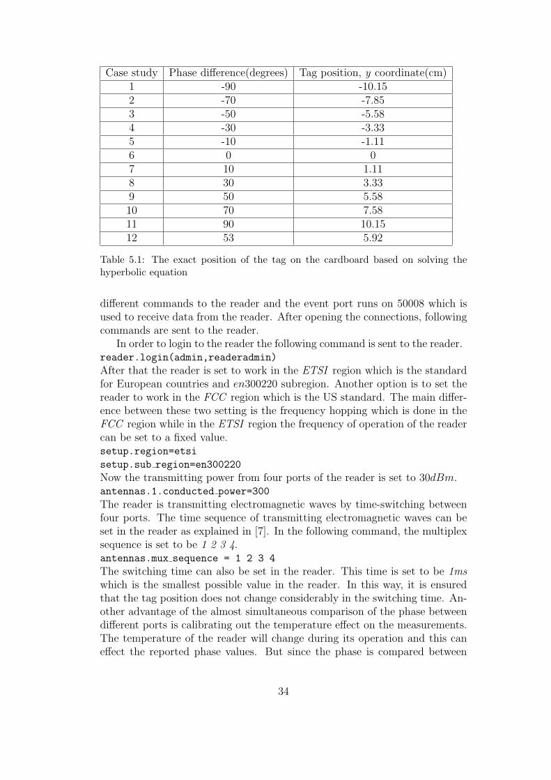
Case study Phase difference(degrees) Tag position, y coordinate(cm)1 -90 -10.152 -70 -7.853 -50 -5.584 -30 -3.335 -10 -1.116 0 07 10 1.118 30 3.339 50 5.5810 70 7.5811 90 10.1512 53 5.92

Table 5.1: The exact position of the tag on the cardboard based on solving thehyperbolic equation

different commands to the reader and the event port runs on 50008 which isused to receive data from the reader. After opening the connections, followingcommands are sent to the reader.

In order to login to the reader the following command is sent to the reader.reader.login(admin,readeradmin)

After that the reader is set to work in the ETSI region which is the standardfor European countries and en300220 subregion. Another option is to set thereader to work in the FCC region which is the US standard. The main differ-ence between these two setting is the frequency hopping which is done in theFCC region while in the ETSI region the frequency of operation of the readercan be set to a fixed value.setup.region=etsi

setup.sub region=en300220

Now the transmitting power from four ports of the reader is set to 30dBm.antennas.1.conducted power=300

The reader is transmitting electromagnetic waves by time-switching betweenfour ports. The time sequence of transmitting electromagnetic waves can beset in the reader as explained in [7]. In the following command, the multiplexsequence is set to be 1 2 3 4.antennas.mux sequence = 1 2 3 4

The switching time can also be set in the reader. This time is set to be 1mswhich is the smallest possible value in the reader. In this way, it is ensuredthat the tag position does not change considerably in the switching time. An-other advantage of the almost simultaneous comparison of the phase betweendifferent ports is calibrating out the temperature effect on the measurements.The temperature of the reader will change during its operation and this caneffect the reported phase values. But since the phase is compared between

34

−100 −50 0 50 100−15

−10

−5

0

5

10

15

Phase difference between antenna one and two (degrees)

y co

ordi

nate

of t

ag p

osito

in (

cm)

Figure 5.3: The exact y coordinate of the tag position versus phase difference be-tween antenna one and two based on solving the hyperbolic equation

ports in close time slots the temperate is the same for the measurements indifferent ports and this will cancel out the effect of the temperature change onthe phase measurements.antennas.check.time=1

In the following command the tag reporting fields are set to transmitting an-tenna, frequency, phase and RSSI.tag.reporting.report fields=antenna freq phase rssi

Now active mode is set which starts transmitting electromagnetic waves fromthe reader.setup.operating mode=active

Now the tag report event is registered in the reader which makes the readerto start sending out the data.reader.events.register(id=21,name=event.tag.report)

35

5.2.2 Receiving and analyzing the phase data to refreshthe cursor position

After registering the tag report event, the program starts to read data fromthe reader. In each iteration 12 data lines are read from the reader. Thismeans that 3 phase data is received for the signal in each port. These phasedata are extracted from the received data from the reader and converted tovalues between 0 and 180 degrees as explained in the previous chapters. Thenthe average value for the phase data is used to calculate the phase differencebetween antenna one and antenna two and also between antenna three andantenna four. After that the phase difference data are scaled between −90degrees and 90 degrees as explained before.

After calculating the average phase difference value in each iteration, theposition of the cursor is calculated using a linear transformation as shownbelow. The aim of this experiment is to control the cursor position on thecomputer screen based on the tag position in y and z directions in the space.The phase difference between antenna one and antenna two gives the positionof the tag in the y direction which will be mapped to the horizontal positionof the cursor while the phase difference between antenna three and antennafour gives tag position in the z direction which will be mapped to the verti-cal position of the cursor. The following commands will transform the phasedifference data to integer numbers which represent the cursor position in thehorizontal and vertical direction.int x position = Convert.ToInt32(Math.Floor((avg phase12 diff + 90)

* 7.6));

int y position = Convert.ToInt32(Math.Floor((avg phase34 diff + 90)

* 5.9));

Then the cursor position is refreshed in every iteration using the followingcommand.Cursor.Position = new Point(x position, y position);

The refresh rate for the mouse cursor or the execution time for each iteration inthe program is measured to be almost 75ms using 3 values for averaging overthe phase data from the reader. This execution time is mainly determined bythe speed of the receiving data from the reader. Having 75ms for the refreshtime ensures that the cursor position is following the tag position almost inrealtime which is shown to be enough for writing with RFID pen by movingthe tag in the air as demonstrated in Figure 5.2.

5.3 Introducing a security model for human

identity verification using RFID tags

There are mainly two counterfeit attacks that can be done in RFID systems asare addressed in [8]. The first attack is RFID IC cloning in which a counterfeitIC can be built to have the same ID of the tag which is to be counterfeited.

36

A solution to this problem is to fabricate PUF-based RFID IC which are notclonable due to the randomness in the manufacturing process as explainedin [8]. The other counterfeit attack is replay attack where an unauthorizeduser listen to the communication between the tag and the reader and producethe same response to the reader as a real tag. These counterfeit systemscan send back any tag ID to the reader and there is not any possible wayfor the reader to distinguish the real tag with the counterfeit attempt. Thiscan lead to identity theft problem in systems where RFID tags are used forhuman identity verification. It is however possible to use encryption in datacommunication between tags and the reader to overcome the replay attackbut a secure encryption will require lots of computational power and hence apower source which is not available in passive tags.

In this section, it is shown how the realtime RFID positioning system de-veloped in this thesis can overcome the replay attack. The reason for immunityof this system against replay attack is that it is technically impossible to builda counterfeit system to send the tag ID to the reader and at the same time beable to control the cursor on the screen when placed in front of the antennaarray of the system. The security of the system is based on the fact thatthe cursor control is done through receiving phase data from four antennasin different time slots. For a counterfeit system to be able to fake a tag IDand control the cursor movement at the same time, it has to send back an RFsignal with appropriate phase to all four antennas at all time slots while thetransmitting sequence by which the reader is switching in time between fourantennas is unknown to the counterfeit system. It is not technically possibleto determine which antenna is transmitting the signal in a short time slot andthen transmit a counterfeit signal with the right phase to the right antennain the same time slot. This means that it is only the movement of the actualRFID tag that can control the cursor position on the computer screen.

The security model can be summarized in this way. After recognizing theidentity of the person based on the ”nonclonable” PUF-based tag ID, thesystem can ask the person to verify his or her identity by clicking on somebuttons on the computer screen. This should be done by moving the cursoron the screen through the tag movement in the air. In this way the presenceof a real tag with the specific ID can be verified by the system.

37

Chapter 6

Conclusion, future work andapplications

In conclusion, the calculation of the tag position based on the phase mea-surements are in good agreement with the actual position of the tag in bothazimuth and elevation directions. Any disagreement between actual positionand calculation is attributed to coupling of nearby objects to electromagneticwaves around the array or the disagreement can be due to the error in thetag placement. As a future work, the system can be used for tag positioningin frequency hopping systems. In this region, the frequency of transmittingsignal is varied randomly and the phase difference data should be calculatedbetween similar frequencies. Then a method should be investigated to usethe phase difference data in different frequencies for finding the tag position.There are several recommendations for improving the operation of system:

1. Some RF absorbing materials can be placed around the array to absorbthe radiation of electromagnetic waves in the unwanted directions. Inthis way the effect of electromagnetic coupling of nearby objects on thephase data will be reduced.

2. Algorithms or methods can be investigated and implemented which canreduce or compensate the effect of the environment on the accuracy ofpositioning.

3. A two dimensional tag like a dual dipole tag can be used instead of dipoletag used in this thesis. In this way, the tag does not need to have someslope in order to be read by four antennas in the array.

4. Some special movement of tag can be defined as mouse click action inthe RFID pen system.

5. A hysteresis method can be applied to the cursor position on the bordersof the screen which corresponds to the borders of the phase ambiguityregion. The problem in these area is multiple cursor jumps to other side

38

of the screen which can be reduced by adding a hysteresis region forcursor position.

Here is a list of some possible applications with some more ideas aboutother possible systems based on the system that is developed in this thesis:

1. The system proposed for human identity confirmation is a reliable andsecure method for human identification. The system can be used for se-cure transactions including but not limited to accessing to secure bank-ing systems, access to the entrance of buildings and opening gates intransportation systems.

2. The secure transactions explained in 1 can be reflected automatically tosocial networks as online status provided that the user is willing to sharehis or her activities on these networks.

3. The drawing of the signature of each person using the RFID pen systemcan be stored in a data base as a transaction confirmation wheneverneeded.

4. The RFID reader can be attached to the array as a hand-held device, tosearch for tags by turning the array to different directions and lookingat the realtime phase difference data on a screen.

5. The antenna array can mechanically track a tag by placing the array ontop of a stepper motor. This system can also be used to scan an area tofind the position of all the tags in the area.

6. The antenna array can electronically scan the beams and find the loca-tion of tags in a large area.

7. The position of the tag can be determined in three dimensions by addingtwo more antennas. 3-D tag positioning system can be used to draw threedimensional objects, or can be used as a new human to computer inter-face having many applications like picking up objects in virtual stores.

8. The tag positioning system can be used as a game console by attachingtags to special gloves or other holders which can be used in differentgames.

9. The RFID pen system can be used as a pen to draw and write in thelectures and presentations.

10. By using two separated systems and triangulation method the positionof tags can be calculated in a reference system. For clarification, thehyperbolic functions discussed in the thesis turn to straight lines whichshow the direction of arrival of tag signal for different phase differencedata.

39

11. A combination of phase mono-pulse and amplitude mono-pulse systemcan be used to clear the phase ambiguity region for tags.

12. Two or more tags can simultaneously control different cursors on a com-puter screen. This can be done by moving each tag in a different phaseclarity region. In this way tags will not collide and will not couple toeach other. The system is specially interesting for game console in gameswith more than one player.

40

Bibliography

[1] D. M. Dobkin, The RF in RFID, Passive UHF RFID in Practice. Oxford:Elsevier Inc., 2008, pp. 42-54.

[2] A. Bensky, Wireless Positioning Technologies and Applications. Norwood,MA: Artech House, 2008, pp. 27-32

[3] ”Application Note for Tag Phase Reporting Technology,” [On-line]. Available: http://www.sirit.com/Tech Support Downloads/Sirit Application Note Tag Phase Reporting.pdf. [Accessed: Dec. 1,2009].

[4] M. Modaresi, ”Design and Fabrication of a High-gain Microstrip-fed Yagi-Uda antenna,” M.Sc. thesis, KTH University, Stockholm, Sweden, 2005.

[5] B. J. Edward and D. F. Rees, ”Microstrip fed printed dipole with an inte-gral balun,” U.S. Patent 4825220, April 25, 1989.

[6] E. Hammerstad and Ø. Jensen, Accurate Models for Microstrip Computer-Aided Design, Symposium on Microwave Theory and Techniques, pp. 407-409, June 1980.

[7] ”INfinity 510 Protocol Reference Guide,” [Online]. Available:http://www.sirit.com/Tech Support Downloads/INfinity 510 Prot Ref Gd v3.0.pdf.[Accessed: Dec. 1, 2009].

[8] S. Devadas, E. Suh, S. Paral, R. Sowell, T. Ziola, and V. Khandelwal,Design and implementation of PUF-based ”unclonable” RFID ICs for anti-counterfeiting and security applications, IEEE International Conference onRFID (Frequency Identification), IEEE RFID 2008, pp. 58-64, April 2008.

41

APPENDIX A

As it is explained before, in order to find y and z coordinates of the tag, equa-tions (3.11) and (3.12) should be used in equation (3.1). Also equations (3.13)and (3.14) should be used in equation (3.6). Then these two equations can besolved to get y and z having x = 57cm. However, in order to find the y value,it can be assumed that z = 0.

In this appendix, it is shown this assumption will introduce a relativeeffective error on the phase difference data which is maximum 16% percent forthe measurement setup used in this thesis.

In order to show this, it is assumed that the tag is placed at point A and thedistances of the tag to antenna one and antenna two are d1 and d2 respectively.

In order to find the y-coordinate of the tag, it is assumed that z = 0. Theprojection of point A on the xy plane is named A′ and the distances of point A′

to antenna one and antenna two are named d′1 and d′2. The following equationrelates these values:d′1

2 − d′22 = d1

2 − d22 which can be rewritten as:

∆d′ = d1+d2d′1+d′2

∆d

The relative error in ∆d∆d′

is directly related to the relative error in ∆Θ∆Θ′ .

The maximum value for d1+d2d′1+d′2

occurs on the borders of phase clarity region.

For the dimensions in the measurement setup in this thesis the maximum errorcan occur if the position of points A and A′ are A = (57, 10.15, 10.5) andA′ = (57, 10.15, 0). The phase center of antenna one is located at (2, 12.15, 0)and the phase center of antenna two is located at (2,−12.15, 0) where alldimensions are in centimeters. These values give, d1 = 63.5cm, d2 = 87.8cm,d′1 = 53cm and d′2 = 77.3cm. So the maximum error in the relative phasedifference introduced with the above assumption is equal to:

Error = |1− d1+d2d′1+d′2

| = 16%

The error in the relative phase difference will also directly translate to theerror in the tag positioning based on the explanations in previous chapters.

42

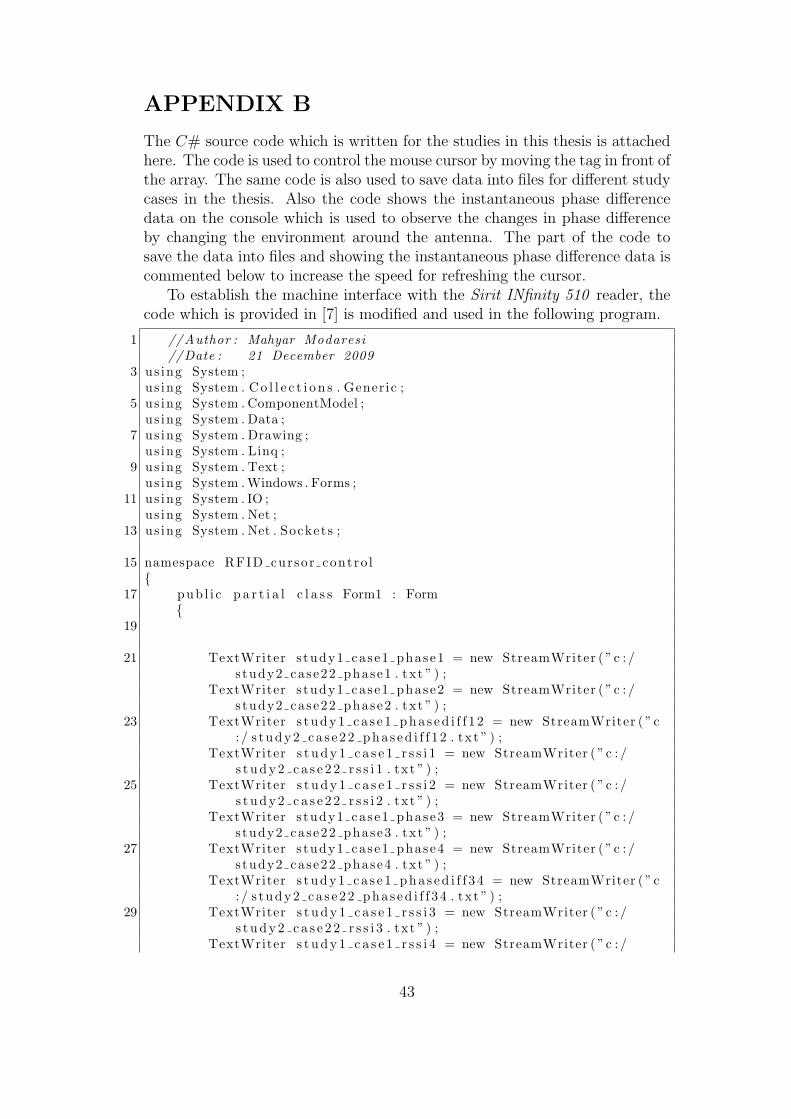
APPENDIX B

The C# source code which is written for the studies in this thesis is attachedhere. The code is used to control the mouse cursor by moving the tag in front ofthe array. The same code is also used to save data into files for different studycases in the thesis. Also the code shows the instantaneous phase differencedata on the console which is used to observe the changes in phase differenceby changing the environment around the antenna. The part of the code tosave the data into files and showing the instantaneous phase difference data iscommented below to increase the speed for refreshing the cursor.

To establish the machine interface with the Sirit INfinity 510 reader, thecode which is provided in [7] is modified and used in the following program.

1 //Author : Mahyar Modaresi//Date : 21 December 2009

3 us ing System ;us ing System . Co l l e c t i o n s . Generic ;

5 us ing System . ComponentModel ;us ing System . Data ;

7 us ing System . Drawing ;us ing System . Linq ;

9 us ing System . Text ;us ing System .Windows . Forms ;

11 us ing System . IO ;us ing System . Net ;

13 us ing System . Net . Sockets ;

15 namespace RFID cursor contro l

17 pub l i c p a r t i a l c l a s s Form1 : Form

19

21 TextWriter s tudy1 case1 phase1 = new StreamWriter ( ”c : /s tudy2 case22 phase1 . txt ” ) ;

TextWriter s tudy1 case1 phase2 = new StreamWriter ( ”c : /s tudy2 case22 phase2 . txt ” ) ;

23 TextWriter s t udy1 ca s e 1 pha s ed i f f 1 2 = new StreamWriter ( ”c: / s tudy2 ca s e 22 pha s ed i f f 1 2 . txt ” ) ;

TextWriter s t udy 1 c a s e 1 r s s i 1 = new StreamWriter ( ”c : /s t udy2 c a s e 2 2 r s s i 1 . txt ” ) ;

25 TextWriter s t udy 1 c a s e 1 r s s i 2 = new StreamWriter ( ”c : /s t udy2 c a s e 2 2 r s s i 2 . txt ” ) ;

TextWriter s tudy1 case1 phase3 = new StreamWriter ( ”c : /s tudy2 case22 phase3 . txt ” ) ;

27 TextWriter s tudy1 case1 phase4 = new StreamWriter ( ”c : /s tudy2 case22 phase4 . txt ” ) ;

TextWriter s t udy1 ca s e 1 pha s ed i f f 3 4 = new StreamWriter ( ”c: / s tudy2 ca s e 22 pha s ed i f f 3 4 . txt ” ) ;

29 TextWriter s t udy 1 c a s e 1 r s s i 3 = new StreamWriter ( ”c : /s t udy2 c a s e 2 2 r s s i 3 . txt ” ) ;

TextWriter s t udy 1 c a s e 1 r s s i 4 = new StreamWriter ( ”c : /

43

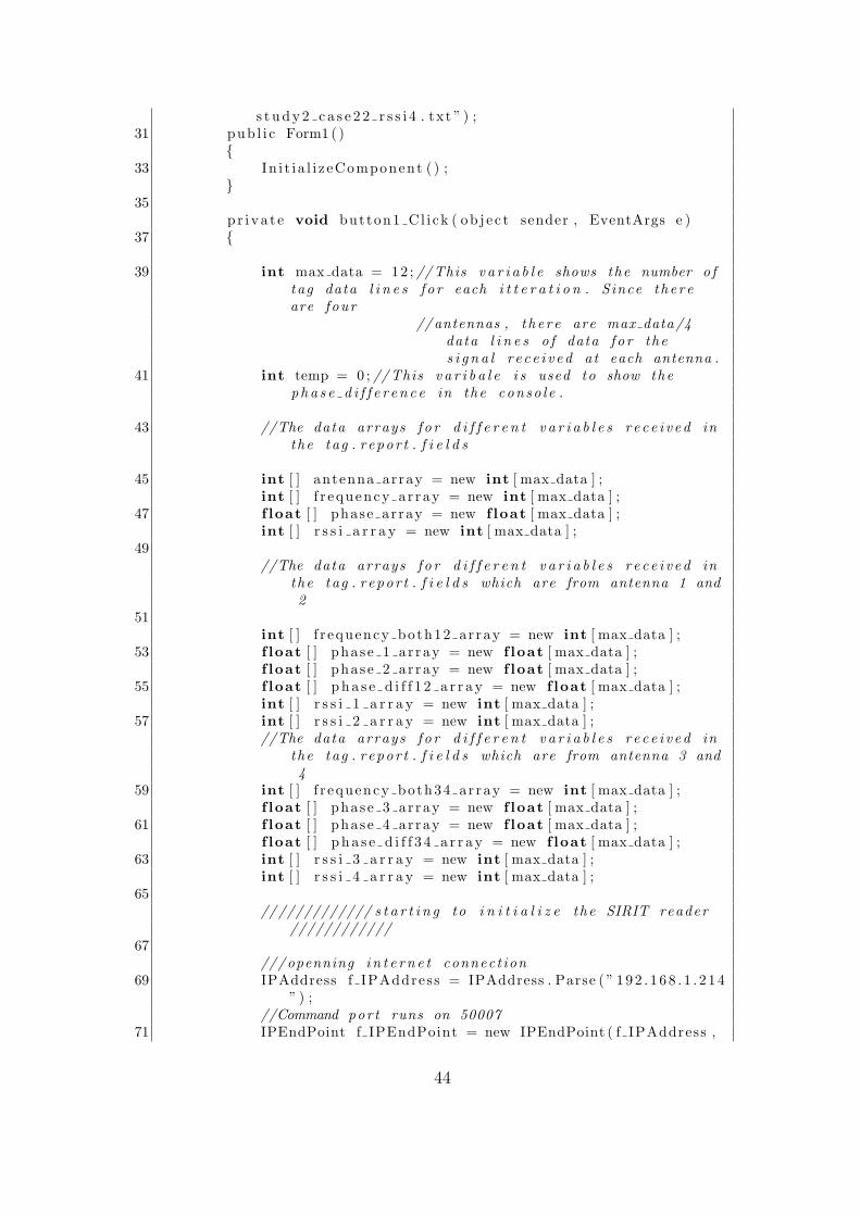
s t udy2 c a s e 2 2 r s s i 4 . txt ” ) ;31 pub l i c Form1 ( )

33 In i t i a l i z eComponent ( ) ;

35

p r i va t e void button1 Cl i ck ( ob j e c t sender , EventArgs e )37

39 int max data = 12 ; //This v a r i a b l e shows the number o ftag data l i n e s f o r each i t t e r a t i o n . Since the r eare four

//antennas , t h e r e are max data/4data l i n e s o f data f o r thes i g n a l r e c e i v ed at each antenna .

41 int temp = 0 ; //This v a r i b a l e i s used to show thep ha s e d i f f e r e n c e in the conso l e .

43 //The data arrays f o r d i f f e r e n t v a r i a b l e s r e c e i v ed inthe tag . r epor t . f i e l d s

45 int [ ] antenna array = new int [ max data ] ;int [ ] f r equency ar ray = new int [ max data ] ;

47 f loat [ ] phase array = new f loat [ max data ] ;int [ ] r s s i a r r a y = new int [ max data ] ;

49//The data arrays f o r d i f f e r e n t v a r i a b l e s r e c e i v ed in

the tag . r epor t . f i e l d s which are from antenna 1 and2

51int [ ] f r equency both12 ar ray = new int [ max data ] ;

53 f loat [ ] phase 1 ar ray = new f loat [ max data ] ;f loat [ ] phase 2 ar ray = new f loat [ max data ] ;

55 f loat [ ] p h a s e d i f f 1 2 a r r a y = new f loat [ max data ] ;int [ ] r s s i 1 a r r a y = new int [ max data ] ;

57 int [ ] r s s i 2 a r r a y = new int [ max data ] ;//The data arrays f o r d i f f e r e n t v a r i a b l e s r e c e i v ed in

the tag . r epor t . f i e l d s which are from antenna 3 and4

59 int [ ] f r equency both34 ar ray = new int [ max data ] ;f loat [ ] phase 3 ar ray = new f loat [ max data ] ;

61 f loat [ ] phase 4 ar ray = new f loat [ max data ] ;f loat [ ] p h a s e d i f f 3 4 a r r a y = new f loat [ max data ] ;

63 int [ ] r s s i 3 a r r a y = new int [ max data ] ;int [ ] r s s i 4 a r r a y = new int [ max data ] ;

65///////////// s t a r t i n g to i n i t i a l i z e the SIRIT reader

////////////67

///openning i n t e r n e t connect ion69 IPAddress f IPAddress = IPAddress . Parse ( ” 192 . 168 . 1 . 2 14

” ) ;//Command por t runs on 50007

71 IPEndPoint f IPEndPoint = new IPEndPoint ( f IPAddress ,

44

Int32 . Parse ( ”50007” ) ) ;Socket m Cl ientsocket = new Socket ( f IPEndPoint .

AddressFamily , SocketType . Stream , ProtocolType . Tcp) ;

73 m Cl ientsocket . Connect ( f IPEndPoint ) ;// event por t runs on 50008

75 IPEndPoint f IPEndPoint2 = new IPEndPoint ( f IPAddress ,Int32 . Parse ( ”50008” ) ) ;

Socket m Cl ientsocket2 = new Socket ( f IPEndPoint2 .AddressFamily , SocketType . Stream , ProtocolType . Tcp) ;

77 m Cl ientsocket2 . Connect ( f IPEndPoint2 ) ;NetworkStream socketStream ;

79 //Create Reader and Writer o b j e c t s to perform h igherl e v e l c a l l s .

socketStream = new NetworkStream ( m Cl ientsocket ) ;81 StreamReader streamReader = new StreamReader (

socketStream ) ;StreamWriter streamWriter = new StreamWriter (

socketStream ) ;83 streamWriter . AutoFlush = true ; // enab l e automatic

f l u s h i n g

85 //Send commands to the reader and r e c e i v e response// l o g i n to the reader

87 streamWriter . WriteLine ( ” reader . l o g i n ( admin , readeradmin) \ r \n” ) ;

s t r i n g responseValue = streamReader . ReadLine ( ) ;89 responseValue = streamReader . ReadLine ( ) ;

91 // s e t t i n g the reader to work in the ETSI reg ionstreamWriter . WriteLine ( ” setup . r eg i on=e t s i \ r \n” ) ;

93 responseValue = streamReader . ReadLine ( ) ;responseValue = streamReader . ReadLine ( ) ;

95 streamWriter . WriteLine ( ” setup . sub reg i on=en300220\ r \n”) ;

responseValue = streamReader . ReadLine ( ) ;97 responseValue = streamReader . ReadLine ( ) ;

99 // s e t t i n g the power f o r antennas 1 2 3 4 to be 30dBmstreamWriter . WriteLine ( ” antennas . 1 . conducted power

=300\ r \n” ) ;101 responseValue = streamReader . ReadLine ( ) ;

responseValue = streamReader . ReadLine ( ) ;103 streamWriter . WriteLine ( ” antennas . 2 . conducted power

=300\ r \n” ) ;responseValue = streamReader . ReadLine ( ) ;

105 responseValue = streamReader . ReadLine ( ) ;streamWriter . WriteLine ( ” antennas . 3 . conducted power

=300\ r \n” ) ;107 responseValue = streamReader . ReadLine ( ) ;

responseValue = streamReader . ReadLine ( ) ;109 streamWriter . WriteLine ( ” antennas . 4 . conducted power

=300\ r \n” ) ;

45

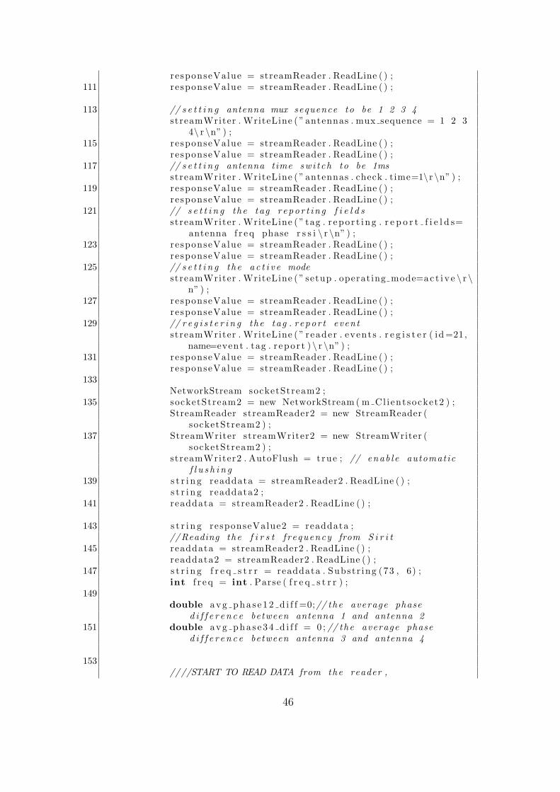
responseValue = streamReader . ReadLine ( ) ;111 responseValue = streamReader . ReadLine ( ) ;

113 // s e t t i n g antenna mux sequence to be 1 2 3 4streamWriter . WriteLine ( ” antennas . mux sequence = 1 2 3

4\ r \n” ) ;115 responseValue = streamReader . ReadLine ( ) ;

responseValue = streamReader . ReadLine ( ) ;117 // s e t t i n g antenna time sw i t ch to be 1ms

streamWriter . WriteLine ( ” antennas . check . time=1\r \n” ) ;119 responseValue = streamReader . ReadLine ( ) ;

responseValue = streamReader . ReadLine ( ) ;121 // s e t t i n g the tag r epo r t i n g f i e l d s

streamWriter . WriteLine ( ” tag . r epo r t i ng . r e p o r t f i e l d s=antenna f r e q phase r s s i \ r \n” ) ;

123 responseValue = streamReader . ReadLine ( ) ;responseValue = streamReader . ReadLine ( ) ;

125 // s e t t i n g the a c t i v e modestreamWriter . WriteLine ( ” setup . operat ing mode=ac t i v e \ r \

n” ) ;127 responseValue = streamReader . ReadLine ( ) ;

responseValue = streamReader . ReadLine ( ) ;129 // r e g i s t e r i n g the tag . r epor t event

streamWriter . WriteLine ( ” reader . events . r e g i s t e r ( id=21,name=event . tag . r epor t ) \ r \n” ) ;

131 responseValue = streamReader . ReadLine ( ) ;responseValue = streamReader . ReadLine ( ) ;

133NetworkStream socketStream2 ;

135 socketStream2 = new NetworkStream ( m Cl ientsocket2 ) ;StreamReader streamReader2 = new StreamReader (

socketStream2 ) ;137 StreamWriter streamWriter2 = new StreamWriter (

socketStream2 ) ;streamWriter2 . AutoFlush = true ; // enab l e automatic

f l u s h i n g139 s t r i n g readdata = streamReader2 . ReadLine ( ) ;

s t r i n g readdata2 ;141 readdata = streamReader2 . ReadLine ( ) ;

143 s t r i n g responseValue2 = readdata ;//Reading the f i r s t f requency from S i r i t

145 readdata = streamReader2 . ReadLine ( ) ;readdata2 = streamReader2 . ReadLine ( ) ;

147 s t r i n g f r e q s t r r = readdata . Substr ing (73 , 6) ;int f r e q = int . Parse ( f r e q s t r r ) ;

149double avg pha s e 12 d i f f =0;// the average phase

d i f f e r e n c e between antenna 1 and antenna 2151 double avg pha s e 34 d i f f = 0 ; // the average phase

d i f f e r e n c e between antenna 3 and antenna 4

153////START TO READ DATA from the reader ,

46

155 /// c a l c u l a t e the average phase d i f f e r e n c e betweenantennas 1 and 2 and antennas 3 and 4/

///and r e f r e s h i n g the mouse cursor acco rd ing l y .157 while ( t rue )

159 int i =0;

int j = 0 ;161

int count = 0 ;163 responseValue2 = ”” ;

//Reading max data l i n e s o f data from the reader165 while ( count < max data − 1)

167

readdata = streamReader2 . ReadLine ( ) ;169 readdata2 = streamReader2 . ReadLine ( ) ;

171 responseValue2 += readdata + Convert . ToChar(13) ;

count++;173

175 s t r i n g da t a s t r i n g = responseValue2 ;

177 s t r i n g a = ” event . tag . r epor t t a g i d=0xAD8A18001C585D9412000091 , antenna=” ; // s i n g l etag on the pen

179 da t a s t r i n g = da t a s t r i n g . Replace ( a , ” tag1 ” ) ;

181 int num array = 0 ; //number o f data in the array

183 //////////EXTRACT INFORMATION FROM da t a s t r i n g tod i f f e r e n t arrays /////////////////////////

for ( j = 0 ; j < max data ; j++)185

i f ( d a t a s t r i n g == ”” )187 break ;

189 int index = da t a s t r i n g . IndexOf ( ” tag ” , 0 ,d a t a s t r i n g . Length , StringComparison .Ordinal ) ;

191 s t r i n g antenna s t r = da t a s t r i n g . Subst r ing (index + 4 , 1) ;

193 i f ( ( antenna s t r == ”1” ) | | ( antenna s t r == ”2” ) | | ( antenna s t r == ”3” ) | | ( antenna s t r== ”4” ) )

195 num array++;

antenna array [ num array ] = int . Parse (antenna s t r ) ;

197

47

else199 break ;

///Now e x t r a c t i n g the f requency201 ///

s t r i n g f r e q s t r = da t a s t r i n g . Subst r ing ( index+ 17 , 6) ;

203 i f ( f r e q s t r == ”869525” )

205 f r equency ar ray [ num array ] = int . Parse( f r e q s t r ) ;

207

else break ;209

////Now e x t r a c t i n g the phase211 s t r i n g pha s e s t r = da t a s t r i n g . Substr ing ( index

+ 33 , 4) ;i f ( pha s e s t r . Length == 4)

213 phase array [ num array ] = Convert .

ToInt32 ( phase s t r , 16) ;215

217 else break ;

219 ///Now co r r e c t i n g the two ’ s complement s i gnand normal i z ing

i f ( phase array [ num array ] > 32768)221 phase array [ num array ] = phase array [

num array ] − 32768 ;

223 // normal i z ing phase

225 phase array [ num array ] = ( f loat ) (phase array [ num array ] / 32768) ∗ 180 ;

227 ////Now e x t r a c t i n g the r s s is t r i n g r s s i s t r = da t a s t r i n g . Subst r ing ( index

+ 45 , 3) ;229

i f ( d a t a s t r i n g . Subst r ing ( index + 44 , 1) == ”−” )

231 r s s i a r r a y [ num array ] = −int . Parse (

r s s i s t r ) ;233

else break ;235 ///Discarding the f i r s t l i n e o f d a t a s t r i n g

a f t e r e x t r a c t i n g the data from the f i r s tl i n e

da t a s t r i n g = da t a s t r i n g . Subst r ing ( index +49 , d a t a s t r i n g . Length − index − 49) ;

237

48

239 //////////////////Now working on the arrays o fdata to f i l l t he data in new arrays f o rd i f f e r e n t antenna data ///////////////

241 int index2 = 0 ;for ( i = 0 ; i < max data ; i++)

243 for ( j = 0 ; j < max data ; j++)

245 i f ( ( ( antenna array [ i ] == 1) && (

antenna array [ j ] == 2) ) && (f r equency ar ray [ i ] == f r equency ar ray [j ] ) )

247 phase 1 ar ray [ index2 ] = phase array [ i

] ;249 phase 2 ar ray [ index2 ] = phase array [ j

] ;f r equency both12 ar ray [ index2 ] =

f r equency ar ray [ i ] ;251 r s s i 1 a r r a y [ index2 ] = r s s i a r r a y [ i ] ;

r s s i 2 a r r a y [ index2 ] = r s s i a r r a y [ j ] ;253 index2 = index2 + 1 ;

255 antenna array [ i ] = 0 ;antenna array [ j ] = 0 ;

257

259 i f ( ( ( antenna array [ i ] == 2) && (antenna array [ j ] == 1) ) && (f r equency ar ray [ i ] == f r equency ar ray [j ] ) )

261 phase 2 ar ray [ index2 ] = phase array [ i

] ;phase 1 ar ray [ index2 ] = phase array [ j

] ;263 f r equency both12 ar ray [ index2 ] =

f r equency ar ray [ i ] ;r s s i 2 a r r a y [ index2 ] = r s s i a r r a y [ i ] ;

265 r s s i 1 a r r a y [ index2 ] = r s s i a r r a y [ j ] ;index2 = index2 + 1 ;

267 antenna array [ i ] = 0 ;antenna array [ j ] = 0 ;

269

271 i f ( ( ( antenna array [ i ] == 3) && (antenna array [ j ] == 4) ) && (f r equency ar ray [ i ] == f r equency ar ray [j ] ) )

273 phase 3 ar ray [ index2 ] = phase array [ i

] ;phase 4 ar ray [ index2 ] = phase array [ j

49

] ;275 f r equency both34 ar ray [ index2 ] =

f r equency ar ray [ i ] ;r s s i 3 a r r a y [ index2 ] = r s s i a r r a y [ i ] ;

277 r s s i 4 a r r a y [ index2 ] = r s s i a r r a y [ j ] ;index2 = index2 + 1 ;

279antenna array [ i ] = 0 ;

281 antenna array [ j ] = 0 ;

283 i f ( ( ( antenna array [ i ] == 4) && (

antenna array [ j ] == 3) ) && (f r equency ar ray [ i ] == f r equency ar ray [j ] ) )

285

287 phase 4 ar ray [ index2 ] = phase array [ i] ;

phase 3 ar ray [ index2 ] = phase array [ j] ;

289 f r equency both34 ar ray [ index2 ] =f r equency ar ray [ i ] ;

r s s i 4 a r r a y [ index2 ] = r s s i a r r a y [ i ] ;291 r s s i 3 a r r a y [ index2 ] = r s s i a r r a y [ j ] ;

index2 = index2 + 1 ;293 antenna array [ i ] = 0 ;

antenna array [ j ] = 0 ;295

297

299

//Now Ca l cu l a t i n g the phase d i f f e r e n c e array301

for ( i = 0 ; i < max data ; i++)303

pha s e d i f f 1 2 a r r a y [ i ] = phase 2 ar ray [ i ] −phase 1 ar ray [ i ] ;

305pha s e d i f f 3 4 a r r a y [ i ] = phase 3 ar ray [ i ] −

phase 4 ar ray [ i ] ;307

309 //Now s c a l i n g the phase between −90 and +90

311 for ( i = 0 ; i < max data ; i++)

313 i f ( (Math . Abs ( pha s e d i f f 1 2 a r r a y [ i ] ) > 90) )

315 pha s e d i f f 1 2 a r r a y [ i ] = pha s e d i f f 1 2 a r r a y[ i ] − 180 ∗ Math . Sign (pha s e d i f f 1 2 a r r a y [ i ] ) ;

50

317

319

321 for ( i = 0 ; i < max data ; i++)

323 i f ( (Math . Abs ( pha s e d i f f 3 4 a r r a y [ i ] ) > 90) )

325 pha s e d i f f 3 4 a r r a y [ i ] = pha s e d i f f 3 4 a r r a y[ i ] − 180 ∗ Math . Sign (pha s e d i f f 3 4 a r r a y [ i ] ) ;

327

329

331 // Ca l cu l a t i n g the average in the phase d i f f e r e n c ein the array

333 int phase count12 = 0 ;double sum phase12 d i f f= 0 ;

335 int phase count34 = 0 ;double sum phase34 d i f f = 0 ;

337for ( i = 0 ; i < max data ; i++)

339 i f ( pha s e d i f f 1 2 a r r a y [ i ] != 0)

341

343 sum phase12 d i f f = sum phase12 d i f f +pha s e d i f f 1 2 a r r a y [ i ] ;

345 phase count12++;//////// Saving i n t e r e s t i n g data in t o f i l e s

347

349 // s tudy1 case1 phase1 . WriteLine (phase 1 array [ i ] ) ;

// s tudy1 case1 phase2 . WriteLine (phase 2 array [ i ] ) ;

351 // s t u d y1 ca s e 1 pha s e d i f f 1 2 . WriteLine (p ha s e d i f f 1 2 a r r a y [ i ] ) ;

// s t u d y 1 c a s e 1 r s s i 1 . WriteLine (r s s i 1 a r r a y [ i ] ) ;

353 // s t u d y 1 c a s e 1 r s s i 2 . WriteLine (r s s i 2 a r r a y [ i ] ) ;

355

357i f ( pha s e d i f f 3 4 a r r a y [ i ] != 0)

359 sum phase34 d i f f= sum phase34 d i f f+

pha s e d i f f 3 4 a r r a y [ i ] ;

51

361phase count34++;

363 //////// Saving i n t e r e s t i n g data in t o f i l e s

365 // s tudy1 case1 phase3 . WriteLine (phase 3 array [ i ] ) ;

// s tudy1 case1 phase4 . WriteLine (phase 4 array [ i ] ) ;

367 // s t u d y1 ca s e 1 pha s e d i f f 3 4 . WriteLine (p ha s e d i f f 3 4 a r r a y [ i ] ) ;

// s t u d y 1 c a s e 1 r s s i 3 . WriteLine (r s s i 3 a r r a y [ i ] ) ;

369 // s t u d y 1 c a s e 1 r s s i 4 . WriteLine (r s s i 4 a r r a y [ i ] ) ;

371

373

375/// c a l c u l a t i n g the average phase d i f f e r e n c e

377i f ( ( ! ( phase count12== 0) ) && ( ! ( phase count34 ==

0) ) )379

avg pha s e 12 d i f f = sum phase12 d i f f /phase count12 ;

381 avg pha s e 34 d i f f = sum phase34 d i f f /phase count34 ;

383

//Now c a l c u l a t i n g the p o s i t i o n o f cursor from thephase d i f f e r e n c e data

385

387 int x po s i t i o n = Convert . ToInt32 (Math . Floor ( (avg pha s e 12 d i f f + 90) ∗ 7 . 6 ) ) ;

int y po s i t i o n = Convert . ToInt32 (Math . Floor ( (avg pha s e 34 d i f f + 90) ∗ 5 . 9 ) ) ;

389Cursor . Po s i t i on = new Point ( x po s i t i on , y p o s i t i o n

) ;391 //Showing the va lue f o r phase d i f f e r e n c e between

antenna 1 and 2 in the conso l e//temp++;

393// i f ( temp == 20)

395 ////Console . Write ( a v g p h a s e 1 2 d i f f ) ;

397 //Console . Write (” ”) ;//Console . WriteLine ( a v g p h a s e 3 4 d i f f ) ;

399//temp = 0;

401 //

52

403 // f o r wh i l e ( t rue )

405p r i va t e void Form1 Load ( ob j e c t sender , EventArgs e )

407

409

411 p r i va t e void Form1 FormClosed ( ob j e c t sender ,FormClosedEventArgs e )

413

s tudy1 case1 phase1 . Close ( ) ;415 s tudy1 case1 phase2 . Close ( ) ;

s t udy1 ca s e 1 pha s ed i f f 1 2 . Close ( ) ;417 s t udy1 c a s e 1 r s s i 1 . Close ( ) ;

s t udy 1 c a s e 1 r s s i 2 . Close ( ) ;419

s tudy1 case1 phase3 . Close ( ) ;421 s tudy1 case1 phase4 . Close ( ) ;

s t udy1 ca s e 1 pha s ed i f f 3 4 . Close ( ) ;423 s t udy1 c a s e 1 r s s i 3 . Close ( ) ;

s t udy 1 c a s e 1 r s s i 4 . Close ( ) ;425

427

53

www.kth.se

TRITA-ICT-EX-2010:216