
RFID TAG LOCALIZATION WITH VIRTUAL MULTI-ANTENNA ...
159
ALMA MATER STUDIORUM - UNIVERSIT ` A DI BOLOGNA CAMPUS DI CESENA SCUOLA DI INGEGNERIA E ARCHITETTURA Corso di Laurea Magistrale in Ingegneria Elettronica e delle Telecomunicazioni per l’Energia TITOLO DELLA TESI RFID TAG LOCALIZATION WITH VIRTUAL MULTI-ANTENNA SYSTEMS Tesi in Sistemi di Telecomunicazioni LM Relatore: Chiar.mo Prof. Ing. DAVIDE DARDARI Correlatori: Dott. Ing. NICOL ´ O DECARLI Prof. Ing. ANDREA GIORGETTI Presentata da: FEDERICO BERTI SESSIONE III ANNO ACCADEMICO 2014-2015
-
Upload
khangminh22 -
Category
Documents
-
view
0 -
download
0
Transcript of RFID TAG LOCALIZATION WITH VIRTUAL MULTI-ANTENNA ...
ALMA MATER STUDIORUM - UNIVERSITA DI BOLOGNACAMPUS DI CESENA
SCUOLA DI INGEGNERIA E ARCHITETTURA
Corso di Laurea Magistrale in Ingegneria Elettronica e delleTelecomunicazioni per l’Energia
TITOLO DELLA TESI
RFID TAG LOCALIZATION WITHVIRTUAL MULTI-ANTENNA
SYSTEMSTesi in
Sistemi di Telecomunicazioni LM
Relatore:Chiar.mo Prof. Ing.DAVIDE DARDARI
Correlatori:
Dott. Ing.NICOLO DECARLI
Prof. Ing.ANDREA GIORGETTI
Presentata da:FEDERICO BERTI
SESSIONE III
ANNO ACCADEMICO 2014-2015

Keywords
RFID
Localization
Phase
Multi-antenna
Tag


Alla mia famiglia...


List of Acronyms
3D three dimensional
AOA angle-of-arrival
CW continuous wave
DOA direction-of-arrival
GPS Global Positioning System
IoT Internet of Things
LLRP Low Level Reader Protocol
LOS line-of-sight
NLOS non-line-of-sight
PDOA phase-difference-of-arrival
RFID radio frequency identification
RMSE root mean square error
RSS received signal strength
RV random variable
RX receiver
SNR signal-to-noise ratio
TDOA time-difference-of-arrival
vii

TOA time-of-arrival
TX transmitter
UWB ultra-wide band
WSN wireless sensor networks
viii
Contents
Abstract 1
Introduction 3
1 Localization Methods 7
1.1 Classic Indoor Localization Methods . . . . . . . . . . . . . . 7
1.1.1 Distance Estimation-Based Methods . . . . . . . . . . 8
1.1.2 Scene Analysis-Based Methods . . . . . . . . . . . . . 11
1.1.3 Proximity-Based Methods . . . . . . . . . . . . . . . . 11
1.1.4 Performance Metrics . . . . . . . . . . . . . . . . . . . 11
1.2 RFID Tag . . . . . . . . . . . . . . . . . . . . . . . . . . . . . 12
1.3 RFID Localization Schemes . . . . . . . . . . . . . . . . . . . 13
1.3.1 Distance Estimation . . . . . . . . . . . . . . . . . . . 14
1.3.2 Scene Analysis . . . . . . . . . . . . . . . . . . . . . . 15
1.3.3 Constrain-Based Approach . . . . . . . . . . . . . . . . 17
1.4 RFID-Based Technology . . . . . . . . . . . . . . . . . . . . . 17
1.5 RFID Phase-Based Spatial Identification . . . . . . . . . . . . 19
1.5.1 Time Domain Phase-Difference-of-Arrival (TD-PDOA) 21
1.5.2 Frequency Domain Phase-Difference-of-Arrival
(FD-PDOA) . . . . . . . . . . . . . . . . . . . . . . . . 21
1.5.3 Spatial Domain Phase-Difference-of-Arrival (SD-PDOA) 21
1.5.4 Synthetic Aperture Radar and Holographic Localization 22
1.6 RFID-UWB technology . . . . . . . . . . . . . . . . . . . . . . 23
2 Localization Algorithms using Virtual Arrays 25
2.1 Virtual Array . . . . . . . . . . . . . . . . . . . . . . . . . . . 25
2.2 Problem Definition . . . . . . . . . . . . . . . . . . . . . . . . 26
ix
2.3 Maximum Likelihood Estimator . . . . . . . . . . . . . . . . . 27
2.3.1 ML Estimator with Constant Amplitudes . . . . . . . . 28
2.3.2 ML Estimator with Variable Amplitudes . . . . . . . . 29
2.4 Holographic Localization Method . . . . . . . . . . . . . . . . 31
3 Simulation Results 33
3.1 Monodimensional Algorithm . . . . . . . . . . . . . . . . . . . 33
3.1.1 Uniformly Spaced Measure Positions . . . . . . . . . . 34
3.1.2 Random Measure Points . . . . . . . . . . . . . . . . . 38
3.1.3 Reader Position with Noise . . . . . . . . . . . . . . . 39
3.1.4 Relative Position Localization . . . . . . . . . . . . . . 43
3.1.5 Not Central Tag Position . . . . . . . . . . . . . . . . . 46
3.1.6 Signal-to-Noise Ratio Simulation . . . . . . . . . . . . 46
3.1.7 Comparison with ML Criterion . . . . . . . . . . . . . 48
4 Measurement Setup 51
4.1 Hardware and Software . . . . . . . . . . . . . . . . . . . . . . 51
4.1.1 Reader . . . . . . . . . . . . . . . . . . . . . . . . . . . 51
4.1.2 EPC Radio-Frequency Identity Protocols Class-1 Generation-
2 UHF RFID . . . . . . . . . . . . . . . . . . . . . . . 52
4.1.3 LLRP-Low Level Reader Protocol . . . . . . . . . . . . 55
4.1.4 FOSSTRACK LLRP Commander . . . . . . . . . . . . 56
4.1.5 RFID Tag . . . . . . . . . . . . . . . . . . . . . . . . . 64
4.2 Antenna Test . . . . . . . . . . . . . . . . . . . . . . . . . . . 64
5 Measurement Results 73
5.1 Linear trajectory . . . . . . . . . . . . . . . . . . . . . . . . . 73
5.1.1 1D-Localization Results . . . . . . . . . . . . . . . . . 74
5.1.2 2D-Localization Results . . . . . . . . . . . . . . . . . 95
5.2 Angular trajectory . . . . . . . . . . . . . . . . . . . . . . . . 98
6 Conclusions 111
A 1D-Localization Results 113
Acknowledgments 131
x

Bibliography 147
xi

xii

Abstract
In questa tesi si sono valutate le prestazioni di un sistema di localizzazione
multi-antenna di tag radio frequency identification (RFID) passivi in ambi-
ente indoor. Il sistema, composto da un reader in movimento che percorre
una traiettoria nota, ha come obiettivo localizzare il tag attraverso misure
di fase; piu precisamente la differenza di fase tra il segnale di interrogazione,
emesso dal reader, e il segnale ricevuto riflesso dal tag che e correlato alla
distanza tra di essi.
Dopo avere eseguito una ricerca sullo stato dell’arte di queste tecniche e
aver derivato il criterio maximum likelihood (ML) del sistema si e proceduto
a valutarne le prestazioni e come eventuali fattori agissero sul risultato di
localizzazione attraverso simulazioni Matlab.
Come ultimo passo si e proceduto a effettuare una campagna di misure,
testando il sistema in un ambiente reale. Si sono confrontati i risultati di
localizzazione di tutti gli algoritmi proposti quando il reader si muove su una
traiettoria rettilinea e su una traiettoria angolare, cercando di capire come
migliorare i risultati.
1

2
Introduction
In recent years the importance of localizing and tracking objects and people
has grown considerably. Also the birth of the Internet of Things (IoT) and
its expansion, where every object can communicate to each other, caused the
need of interconnect many devices. In this context the information about
their locations could be important.
Simultaneously the technological progress of RFID systems has brought
an enormous diffusion of this technology. Originally they were created for
the purpose of automatically identifying and automatic storage of informa-
tion relevant to objects, animals or people. This technology thanks to its
simplicity, low cost and small dimensions, has found use in many environ-
ments like logistic, airport baggage management, inventory process, security
and access control. A RFID system is composed at least of two devices: a
reader that makes interrogations to the tag and the tag which answers with
its ID by modulating the interrogation. The reader can measures only the
received signal strength (RSS) level of the signal and the phase difference
between the interrogation and the response of the tag.
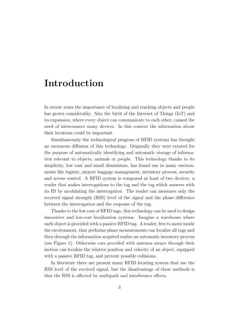
Thanks to the low cost of RFID tags, this technology can be used to design
innovative and low-cost localization systems. Imagine a warehouse where
each object is provided with a passive RFID tag. A reader, free to move inside
the environment, that performs phase measurements can localize all tags and
then through the information acquired realize an automatic inventory process
(see Figure 1). Otherwise cars provided with antenna arrays through their
motion can localize the relative position and velocity of an object, equipped
with a passive RFID tag, and prevent possible collisions.
In literature there are present many RFID locating system that use the
RSS level of the received signal, but the disadvantage of these methods is
that the RSS is affected by multipath and interference effects.
3
Figure 1: Example of localization in a warehouse environment using a moving
reader.
The objective of this thesis is to evaluate the performance and how im-
prove it of a RFID localization system formed by a reader, moving in a known
trajectory, that performs phase measurements.
This work is organized as follows:
- Chapter 1: describes the principal indoor localization techniques and
the architecture of RFID-based technologies. Also the principal RFID
phase-based spatial identification methods are introduced.
- Chapter 2: contains a mathematical analysis in order to derive the ML
criterion of the system and describes the algorithms proposed.
- Chapter 3: this chapter collects the simulation results of our system ob-
tained through Matlab simulators in order to discover the performance
and the features of the locating system implemented.
- Chapter 4: shows the measurement setup adopted and the principal
standard protocols that are used in RFID technologies.
- Chapter 5: describes the measurement campaign carried out in a real
indoor environment and compares the localization result of the different
algorithms investigation, trying to minimize the root mean square error
(RMSE).
- Chapter 6: reports the conclusions of the work.
4

This thesis has been carried out within the European project XCYCLE.
Its objective is to reduce accidents and fatalities of cyclists in urban traffic
and improve its comfort. XCYCLE has an objective of developing user-
friendly, technology-based systems to make cycling safer in traffic [1].
RFID localization technologies could be used in this contest, for example,
to localize cyclists at junctions and prevent possible collisions.
XCYCLE consortium is composed by: Alma Mater Studiorum-University
of Bologna, ITS-University of Leeds, Volvo Group, DLR Germany, University
of Groningen, VTI, Imtech, Kite Solutions and Jenoptik.
5

6
Chapter 1
Localization Methods
1.1 Classic Indoor Localization Methods
The localization methods are processes that perform physical measurements,
like distances or angles, in order to find the exact position of a mobile de-
vice [2]. A locating system is composed at least by: mobile devices or target
that are moving in an area; base stations at known positions and data process-
ing subsystems. Propagation in indoor environment is affected by many prob-
lems like multipath, diffraction, reflection, non-line-of-sight (NLOS) path and
absorption [4]. There are several localization methods in literature [5]. The
methods can be divided into three classes: distance-based estimation, scene
analysis based and proximity-based [6].
Distance estimation methods can be divided into:
• Received Signal Strength (RSS);
• Time-of-Arrival (TOA);
• Time-Difference-of-Arrival (TDOA);
• Received Signal Phase (RSP);
• Angle of Arrival (AOA);
Scene analysis methods can be divided into:
• k-Nearest-Neighbor (kNN);
• Probabilistic Approaches.
7
CHAPTER 1. LOCALIZATION METHODS
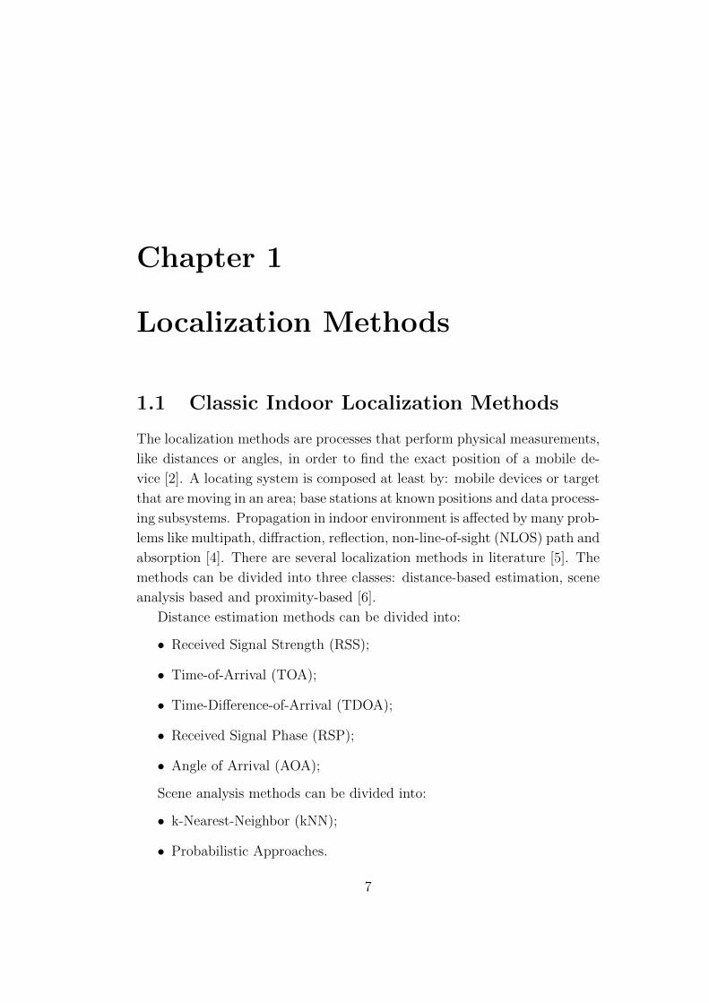
Figure 1.1: RFID-based localization system [3].
1.1.1 Distance Estimation-Based Methods
These algorithms use a triangulation or lateration approach to estimate the
mobile device location. They convert physical measurements of the system,
like propagation time or received power, in equivalent distance values.
• RSS-Received Signal Strength Method: Technique based on the
measure of the power of the signal received at the reader/base station.
The distance measurement can be obtained knowing the path-loss of the
radio channel. The attenuation of the signal is function of the distance
between the transmitter and the receiver. Therefore, the device with
unknown position is placed on a circumference with radius equal to
the distance estimated. Having at least three base stations or readers
doing the RSS measure it is possible estimate the position of the device
resolving a triangulation problem. This method is very sensitive to
shadowing and multipath effects; they can cause a large distance error
that determines a wrong localization.
• TOA-Time of Arrival Method: Technique based on the measure of
the signal propagation time between base stations and the mobile device
with unknown position. The distance measurement can be obtained
from the time measurement knowing the propagation speed of the sig-
nal. Therefore, the device with unknown position should be placed on
a circumference with radius equal to the distance estimated. Having
8
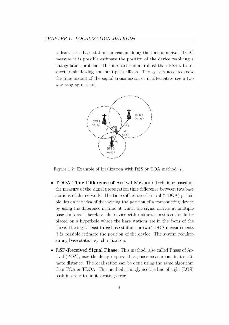
CHAPTER 1. LOCALIZATION METHODS
at least three base stations or readers doing the time-of-arrival (TOA)
measure it is possible estimate the position of the device resolving a
triangulation problem. This method is more robust than RSS with re-
spect to shadowing and multipath effects. The system need to know
the time instant of the signal transmission or in alternative use a two
way ranging method.
Figure 1.2: Example of localization with RSS or TOA method [7].
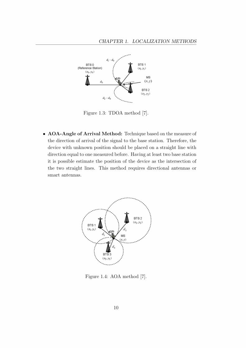
• TDOA-Time Difference of Arrival Method: Technique based on
the measure of the signal propagation time difference between two base
stations of the network. The time-difference-of-arrival (TDOA) princi-
ple lies on the idea of discovering the position of a transmitting device
by using the difference in time at which the signal arrives at multiple
base stations. Therefore, the device with unknown position should be
placed on a hyperbole where the base stations are in the focus of the
curve. Having at least three base stations or two TDOA measurements
it is possible estimate the position of the device. The system requires
strong base station synchronization.
• RSP-Received Signal Phase: This method, also called Phase of Ar-
rival (POA), uses the delay, expressed as phase measurements, to esti-
mate distance. The localization can be done using the same algorithm
than TOA or TDOA. This method strongly needs a line-of-sight (LOS)
path in order to limit locating error.
9
CHAPTER 1. LOCALIZATION METHODS
Figure 1.3: TDOA method [7].
• AOA-Angle of Arrival Method: Technique based on the measure of
the direction of arrival of the signal to the base station. Therefore, the
device with unknown position should be placed on a straight line with
direction equal to one measured before. Having at least two base station
it is possible estimate the position of the device as the intersection of
the two straight lines. This method requires directional antennas or
smart antennas.
Figure 1.4: AOA method [7].
10
CHAPTER 1. LOCALIZATION METHODS
1.1.2 Scene Analysis-Based Methods
Scene analysis approaches have a first step for collecting the fingerprint of
the environment. First of all the ambient is divided into several subareas,
then at each zone a value obtained through preliminary measurements is
assigned, so a database of the area is built. In the second step of the method
the target performs a measure and compares its value with the database
values in order to find the subarea of membership. Generally, RSS-based
fingerprinting is used. The two main techniques are: k-Nearest-Neighbour
(kNN) and probabilistic method.
• k-Nearest-Neighbour (kNN): It consists in a first time measuring
RSS at known location in order to make a database called radio map.
Then a mobile device can perform RSS measurements to find the k
closest matches in the signal space previously built. Finally, a root
mean square algorithm is applied in order to find the estimated location
of the device.
• Probabilistic Approach: This method assumes that there are n
possible locations and one observed strength vector during the sec-
ond phase according to Bayes formula. The location with the highest
probability is chosen.
1.1.3 Proximity-Based Methods
This approach relies on dense deployment of antenna. When the target enters
in the radio range of a single antenna, its position is assumed as the same of
this receiver. If more than one antenna detect the target, the mobile device
is collocated in the position of the receiver with the strongest signal. The
accuracy of this method is equal of the size of the cells.
1.1.4 Performance Metrics
Different applications or technologies may have different requirements on
localization system. There are different performance metric to evaluate in
order to reach a performance objective.
Performance metrics for indoor wireless location systems are [3, 8]:
11
CHAPTER 1. LOCALIZATION METHODS
• Accuracy: In general this parameter evaluates the localization error,
that is the distance between the real position of the target and the
estimated position. This is the most important parameter in these
systems; higher is the accuracy, better is the system but often there is
a trade off between this parameter and other performance metrics.
• Precision: This parameter is an indicator of how uniformly the sys-
tem works. Accuracy only evaluates the mean of the distance error.
Precision parameter represents the robustness of the localization tech-
nique i.e., the variations on its performance over many tentative. Many
scientific papers indicate precision as geometric dilution of precision
(GDOP) or location error standard deviation.
• Complexity: It depends from hardware, software and data processing.
• Scalability: The scalability represents how the system can work cor-
rectly in a different environment keeping the same performance.
• Latency: It is an important performance metric to evaluate a local-
ization system. Latency is defined as the time required by the system
to generate the new estimated position when the target moves to a new
location. In real time system it is very important to have a low latency.
• Robustness: A high robustness ensures that a system could work in
complicated environments where there is incomplete information, some
signals are not available, a wireless sensor network with disabled nodes
or high presence of multipath or interference effects.
• Cost: Cost is another performance metric to evaluate when a localiza-
tion system is designed. Costs include money, time, energy, space and
weight.
1.2 RFID Tag
RFID tags, also called transponders or labels, are simple devices formed by
an antenna and an integrated circuit. There are three different type of RFID
tags:
12
CHAPTER 1. LOCALIZATION METHODS
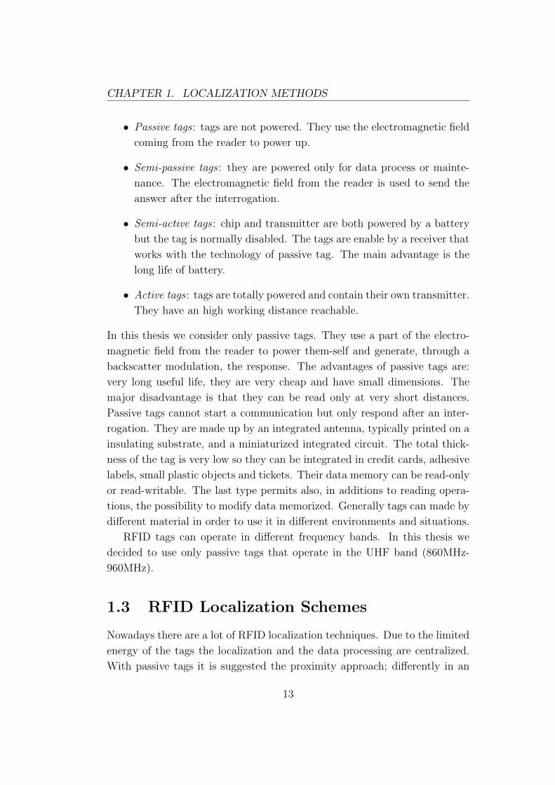
• Passive tags : tags are not powered. They use the electromagnetic field
coming from the reader to power up.
• Semi-passive tags : they are powered only for data process or mainte-
nance. The electromagnetic field from the reader is used to send the
answer after the interrogation.
• Semi-active tags : chip and transmitter are both powered by a battery
but the tag is normally disabled. The tags are enable by a receiver that
works with the technology of passive tag. The main advantage is the
long life of battery.
• Active tags : tags are totally powered and contain their own transmitter.
They have an high working distance reachable.
In this thesis we consider only passive tags. They use a part of the electro-
magnetic field from the reader to power them-self and generate, through a
backscatter modulation, the response. The advantages of passive tags are:
very long useful life, they are very cheap and have small dimensions. The
major disadvantage is that they can be read only at very short distances.
Passive tags cannot start a communication but only respond after an inter-
rogation. They are made up by an integrated antenna, typically printed on a
insulating substrate, and a miniaturized integrated circuit. The total thick-
ness of the tag is very low so they can be integrated in credit cards, adhesive
labels, small plastic objects and tickets. Their data memory can be read-only
or read-writable. The last type permits also, in additions to reading opera-
tions, the possibility to modify data memorized. Generally tags can made by
different material in order to use it in different environments and situations.
RFID tags can operate in different frequency bands. In this thesis we
decided to use only passive tags that operate in the UHF band (860MHz-
960MHz).
1.3 RFID Localization Schemes
Nowadays there are a lot of RFID localization techniques. Due to the limited
energy of the tags the localization and the data processing are centralized.
With passive tags it is suggested the proximity approach; differently in an
13
CHAPTER 1. LOCALIZATION METHODS
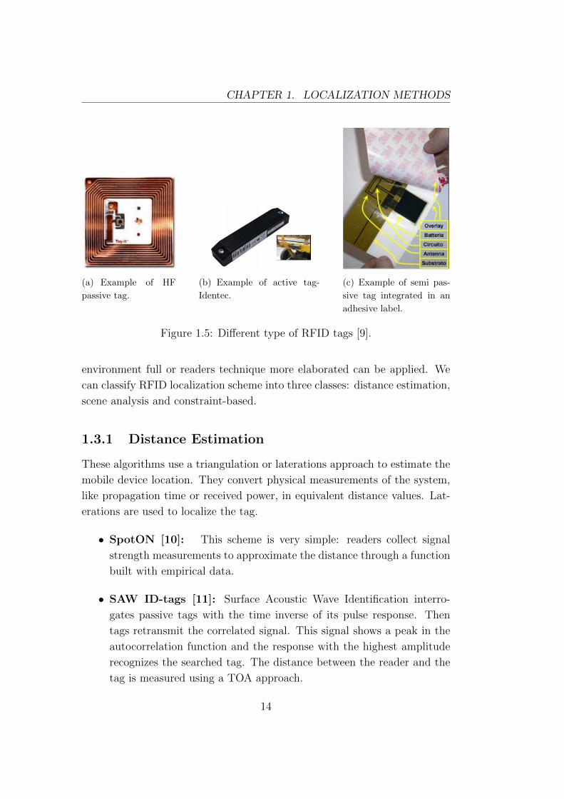
(a) Example of HF
passive tag.
(b) Example of active tag-
Identec.
(c) Example of semi pas-
sive tag integrated in an
adhesive label.
Figure 1.5: Different type of RFID tags [9].
environment full or readers technique more elaborated can be applied. We
can classify RFID localization scheme into three classes: distance estimation,
scene analysis and constraint-based.
1.3.1 Distance Estimation
These algorithms use a triangulation or laterations approach to estimate the
mobile device location. They convert physical measurements of the system,
like propagation time or received power, in equivalent distance values. Lat-
erations are used to localize the tag.
• SpotON [10]: This scheme is very simple: readers collect signal
strength measurements to approximate the distance through a function
built with empirical data.
• SAW ID-tags [11]: Surface Acoustic Wave Identification interro-
gates passive tags with the time inverse of its pulse response. Then
tags retransmit the correlated signal. This signal shows a peak in the
autocorrelation function and the response with the highest amplitude
recognizes the searched tag. The distance between the reader and the
tag is measured using a TOA approach.
14
CHAPTER 1. LOCALIZATION METHODS
• LPM [12]: Local Position Measurement (LPM) readers are synchro-
nized thanks to a reference tag (RT) positioned in fixed location. This
method is based on the TDOA approach. Selective active tags after
an interrogation responds at the time tMT . The time difference tdiff of
the signals between reader Ri and tag can be calculate as:
ctdiff (Ri) = c(tMT − tRT ) + ‖MT −Ri‖ − ‖RT −Ri‖ (1.1)
where c is the speed of light andMT indicates the measurement transpon-
der.
• RSP [13]: Two readers at fixed locations calculate the phase difference
of a moving tag. When they collect a lot of measures the estimation
can be done through a least square fitting technique. With two pairs
of readers it is possible a triangulation to find the tag position and its
direction. It is an example of direction-of-arrival (DOA) method.
1.3.2 Scene Analysis
The principal RFID localization scheme belonging to scene analysis category
found on scientific papers are the following.
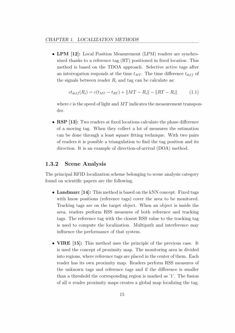
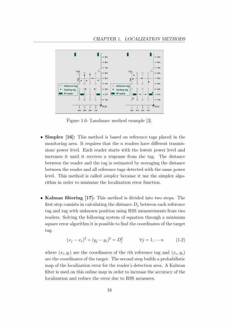
• Landmarc [14]: This method is based on the kNN concept. Fixed tags
with know positions (reference tags) cover the area to be monitored.
Tracking tags are on the target object. When an object is inside the
area, readers perform RSS measures of both reference and tracking
tags. The reference tag with the closest RSS value to the tracking tag
is used to compute the localization. Multipath and interference may
influence the performance of that system.
• VIRE [15]: This method uses the principle of the previous case. It
is used the concept of proximity map. The monitoring area in divided
into regions, where reference tags are placed in the center of them. Each
reader has its own proximity map. Readers perform RSS measures of
the unknown tags and reference tags and if the difference is smaller
than a threshold the corresponding region is marked as ’1’. The fusion
of all n reader proximity maps creates a global map localizing the tag.
15
CHAPTER 1. LOCALIZATION METHODS
Figure 1.6: Landmarc method example [3].
• Simplex [16]: This method is based on reference tags placed in the
monitoring area. It requires that the n readers have different trasmis-
sione power level. Each reader starts with the lowest power level and
increases it until it receives a response from the tag. The distance
between the reader and the tag is estimated by averaging the distance
between the reader and all reference tags detected with the same power
level. This method is called simplex because it use the simplex algo-
rithm in order to minimize the localization error function.
• Kalman filtering [17]: This method is divided into two steps. The
first step consists in calculating the distance Dj between each reference
tag and tag with unknown position using RSS measurements from two
readers. Solving the following system of equation through a minimum
square error algorithm it is possible to find the coordinates of the target
tag.
(xj − xe)2 + (yj − ye)2 = D2j ∀j = 1, · · ·n (1.2)
where (xi, yi) are the coordinates of the ith reference tag and (xe, ye)
are the coordinates of the target. The second step builds a probabilistic
map of the localization error for the reader’s detection area. A Kalman
filter is used on this online map in order to increase the accuracy of the
localization and reduce the error due to RSS measures.
16
CHAPTER 1. LOCALIZATION METHODS
1.3.3 Constrain-Based Approach
The main method that belongs to this category is 3-D Constraints [18]. It is
based on connectivity information and it defines that if a reader can detect
a tag then the distance between them is inferior of the reader’s read range.
The area is discretized into points in order to delimit the detection area of
the readers.
1.4 RFID-Based Technology
Another way to classify RFID systems is depending on their technologies.
It can be classified into four categories: tag based, reader based, transceiver
free and hybrid technologies [3].
• Tag-based technologies
Tag-based technologies require that the target object carry a tag, for
example an active tag that periodically transmits beacon messages. An
example of this technology is LANDMARC system [14]. It use reference
tag in known positions and RSS measurements in order to find or track
a target carrying an active tag. It is very simple to implement but it
suffers of multipath and interference effect.
• Reader-based technologies
In this technologies classical roles of readers and tags are reversed: tags
are placed at known and fixed position and a reader is attached to a ob-
ject or is carried by an user [19]. The position of the user is determined
using tag IDs or RSS value read by the reader. This method is also
called as reverse RFID. It permits to remove the dependence on the
infrastructure of networked readers, very useful in many applications
concerning tracking people in dangerous situations like natural disaster
where the preexisting infrastructure can be damaged.
Active or passive tags can be used with this technology.
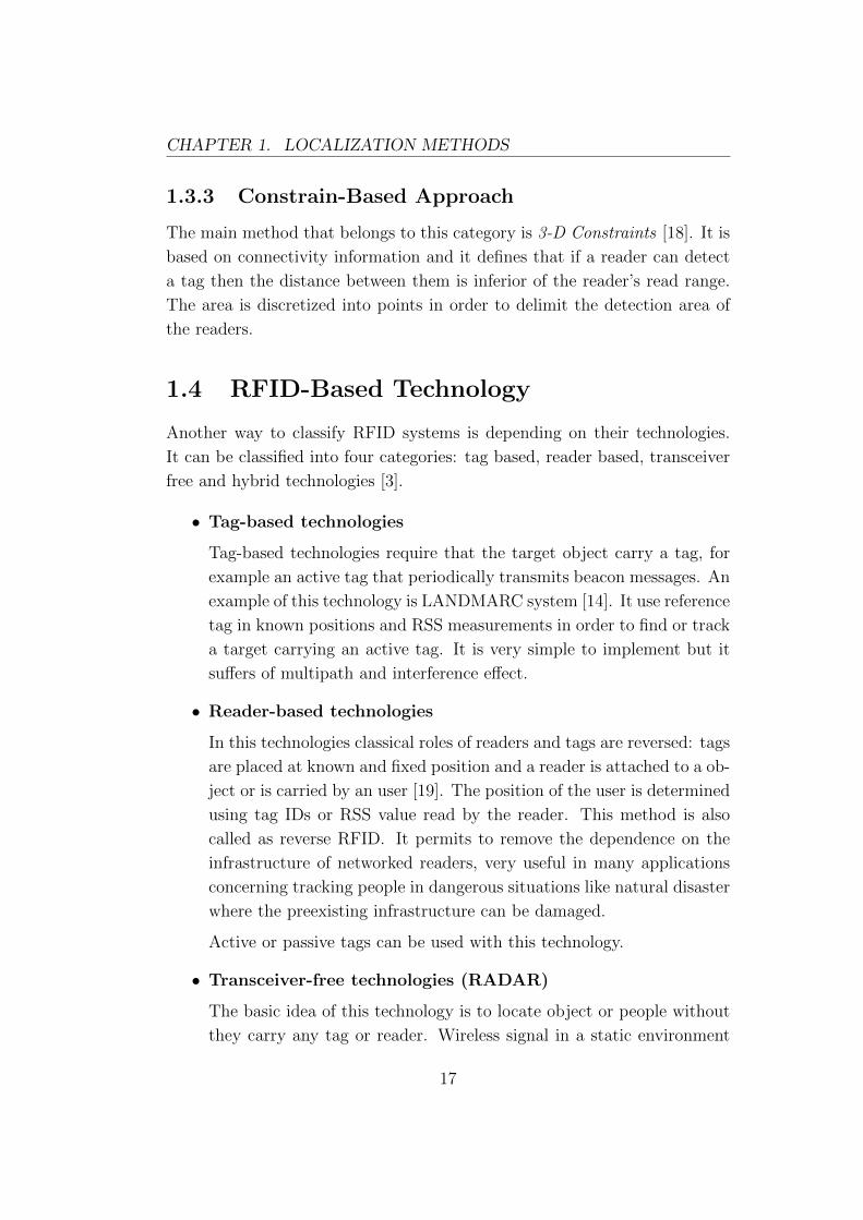
• Transceiver-free technologies (RADAR)
The basic idea of this technology is to locate object or people without
they carry any tag or reader. Wireless signal in a static environment
17
CHAPTER 1. LOCALIZATION METHODS
Figure 1.7: Transceiver-free technologies example [3].
are quite stable. When an object are moving in a monitored area it
cause changes on the signal.
A simple implementation of this technology is the following [20]: an
area is covered with an array of tags and few readers are placed on
the ground. Readers periodically read the RSS value of tags. These
values are stable in a static environment. When an object is moving
in the area it causes changes in the RSS values of nearby tags. This
information it used to track and localize the object. See Figure 1.7.
This algorithm requires a training step where for an amount of time the
system collects RSS values of tags. The main advantage of transceiver-
free technologies is that the target does not carry a device but the
localization and tracking of multiple object are very hard.
• Hybrid technologies
Hybrid technologies try to join advantages of different technologies.
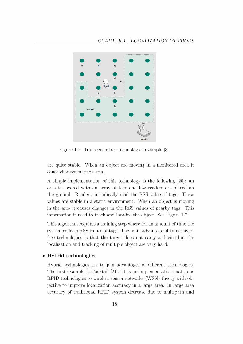
The first example is Cocktail [21]. It is an implementation that joins
RFID technologies to wireless sensor networks (WSN) theory with ob-
jective to improve localization accuracy in a large area. In large area
accuracy of traditional RFID system decrease due to multipath and
18
CHAPTER 1. LOCALIZATION METHODS
Figure 1.8: Cocktail architecture example [3].
interference effects. Cocktail employs a sparse WSN network to cover
the area using reference tags and sensor nodes. Sensor nodes have a
sparse grid deployment respect to tags grid because they are expensive.
When a target is moving in the area it causes changes in RSS values
of some sensor link, called influential links. Influential links tend to be
clustered around the object [22].
The a LANDMARC [14] approach or Support Vector Regression (SVR)
[23] is applied.
Cocktail improve the localization accuracy respect to previous tech-
nologies. However tracking multiple objects is very hard if they are
very close to each other.
The second example is a technology that joins RFID to inertial navi-
gation system (INS) using inertial and non-inertial sensors.
In a hybrid Reverse-RFID/INS system the target carry a reader and a
portable inertial navigation sensor. When the object is out of range of
a tag, the INS is used to track the trajectory. As soon as the object
enter in the read range of a tag, it know coordinates are used to correct
the trajectory estimated. This technology have good results only if the
time spend using the inertial sensor are small.
1.5 RFID Phase-Based Spatial Identification
The previously seen locating system mainly use the RSS indicator or TDOA
measurements. Using UHF RFID tags, RSS measurements could be very
19
CHAPTER 1. LOCALIZATION METHODS
unreliable due to multipath and interference effects or reliable only in a short
distance. Moreover RFID tags and readers cannot operate in short impulse
mode as required by a TOA approach because they are a very short range
narrowband technology.
Thanks to modern RFID readers that perform fully coherent detection
and recover the phase of the tag signal, tag phase information could be used
to determine the position and the velocity of the moving tag. This application
is also called as spatial identification [24].
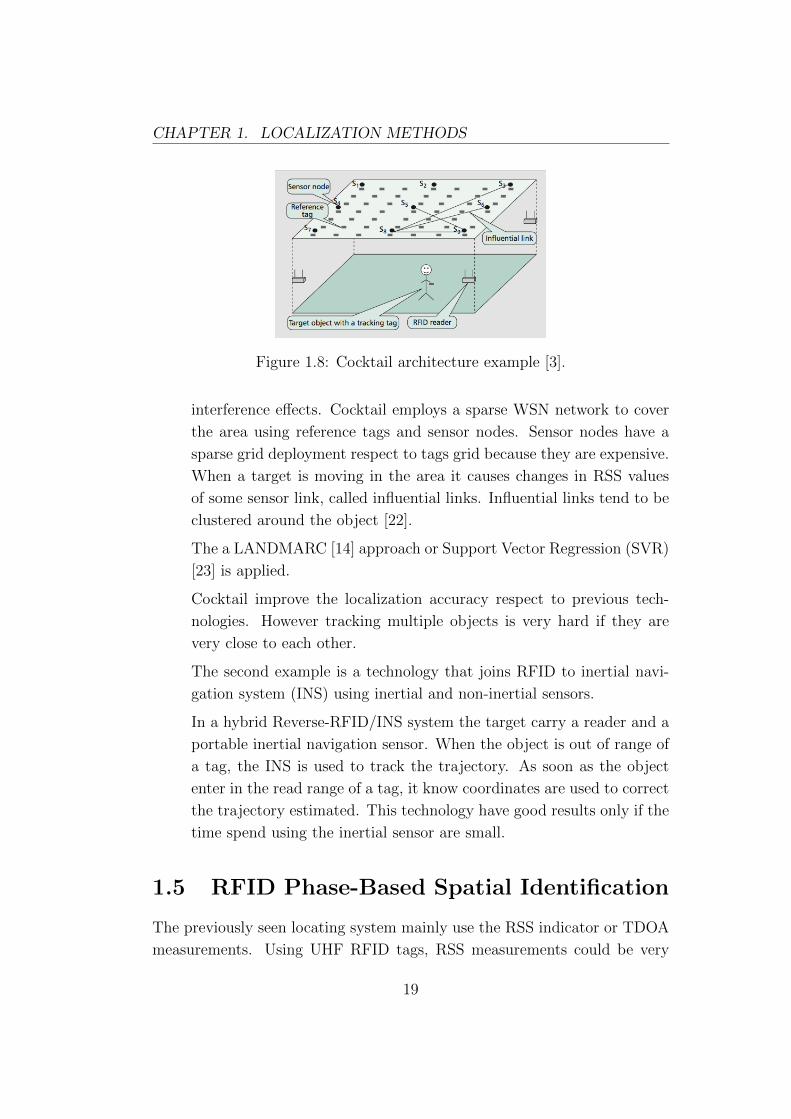
Tag phase information depends from the propagation channel. Using a
phase-difference-of-arrival (PDOA) approach it is possible erase some addi-
tive factors, like the phase introduced by cables or by the hardware, that
affect the phase read by the reader.
Figure 1.9: Phase identification schematic [24] .
The phase of the signal received by the reader is:
ϕd = ϕ+ ϕ0 + ϕBS (1.3)
where ϕ is the phase due to the electromagnetic propagation, ϕ0 is the phase
deriving from cables and other system components and ϕBS is the backscatter
phase from the tag.
ϕ = −22πf
cd (1.4)
where c is the propagation velocity, f is the frequency of the signal and d is
the distance between reader antenna and the tag.
20
CHAPTER 1. LOCALIZATION METHODS
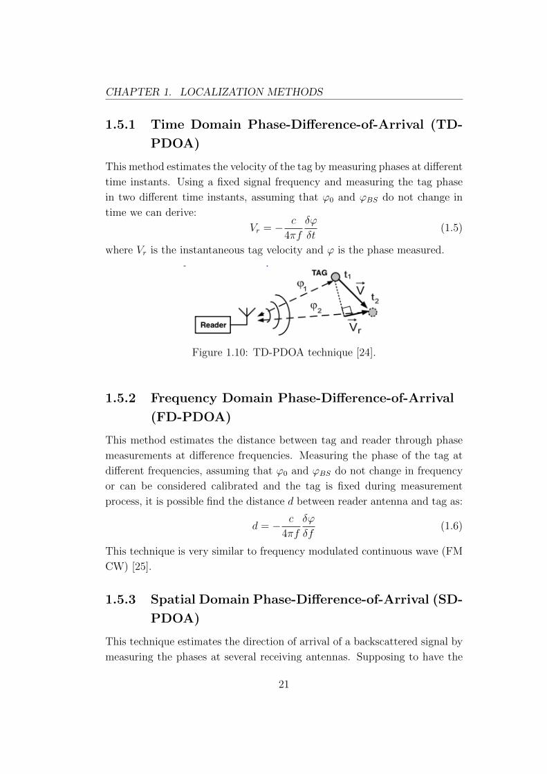
1.5.1 Time Domain Phase-Difference-of-Arrival (TD-
PDOA)
This method estimates the velocity of the tag by measuring phases at different
time instants. Using a fixed signal frequency and measuring the tag phase
in two different time instants, assuming that ϕ0 and ϕBS do not change in
time we can derive:
Vr = − c
4πf
δϕ
δt(1.5)
where Vr is the instantaneous tag velocity and ϕ is the phase measured.
Figure 1.10: TD-PDOA technique [24].
1.5.2 Frequency Domain Phase-Difference-of-Arrival
(FD-PDOA)
This method estimates the distance between tag and reader through phase
measurements at difference frequencies. Measuring the phase of the tag at
different frequencies, assuming that ϕ0 and ϕBS do not change in frequency
or can be considered calibrated and the tag is fixed during measurement
process, it is possible find the distance d between reader antenna and tag as:
d = − c
4πf
δϕ
δf(1.6)
This technique is very similar to frequency modulated continuous wave (FM
CW) [25].
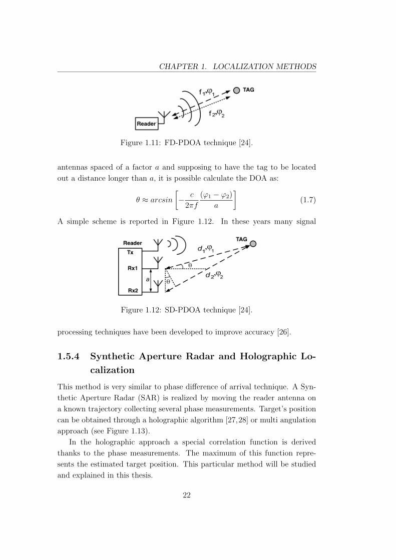
1.5.3 Spatial Domain Phase-Difference-of-Arrival (SD-
PDOA)
This technique estimates the direction of arrival of a backscattered signal by
measuring the phases at several receiving antennas. Supposing to have the
21
CHAPTER 1. LOCALIZATION METHODS
Figure 1.11: FD-PDOA technique [24].
antennas spaced of a factor a and supposing to have the tag to be located
out a distance longer than a, it is possible calculate the DOA as:
θ ≈ arcsin
[− c
2πf
(ϕ1 − ϕ2)
a
](1.7)
A simple scheme is reported in Figure 1.12. In these years many signal
Figure 1.12: SD-PDOA technique [24].
processing techniques have been developed to improve accuracy [26].
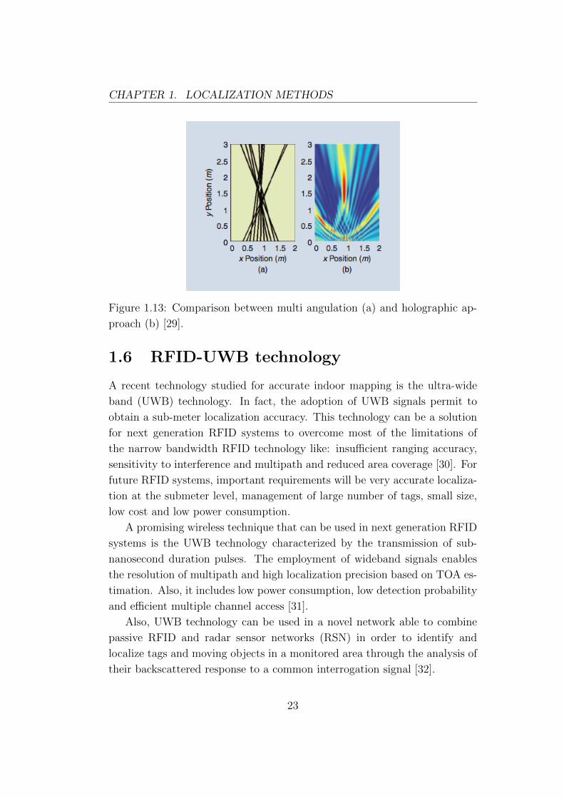
1.5.4 Synthetic Aperture Radar and Holographic Lo-
calization
This method is very similar to phase difference of arrival technique. A Syn-
thetic Aperture Radar (SAR) is realized by moving the reader antenna on
a known trajectory collecting several phase measurements. Target’s position
can be obtained through a holographic algorithm [27,28] or multi angulation
approach (see Figure 1.13).
In the holographic approach a special correlation function is derived
thanks to the phase measurements. The maximum of this function repre-
sents the estimated target position. This particular method will be studied
and explained in this thesis.
22
CHAPTER 1. LOCALIZATION METHODS
Figure 1.13: Comparison between multi angulation (a) and holographic ap-
proach (b) [29].
1.6 RFID-UWB technology
A recent technology studied for accurate indoor mapping is the ultra-wide
band (UWB) technology. In fact, the adoption of UWB signals permit to
obtain a sub-meter localization accuracy. This technology can be a solution
for next generation RFID systems to overcome most of the limitations of
the narrow bandwidth RFID technology like: insufficient ranging accuracy,
sensitivity to interference and multipath and reduced area coverage [30]. For
future RFID systems, important requirements will be very accurate localiza-
tion at the submeter level, management of large number of tags, small size,
low cost and low power consumption.
A promising wireless technique that can be used in next generation RFID
systems is the UWB technology characterized by the transmission of sub-
nanosecond duration pulses. The employment of wideband signals enables
the resolution of multipath and high localization precision based on TOA es-
timation. Also, it includes low power consumption, low detection probability
and efficient multiple channel access [31].
Also, UWB technology can be used in a novel network able to combine
passive RFID and radar sensor networks (RSN) in order to identify and
localize tags and moving objects in a monitored area through the analysis of
their backscattered response to a common interrogation signal [32].
23

CHAPTER 1. LOCALIZATION METHODS
24
Chapter 2
Localization Algorithms using
Virtual Arrays
2.1 Virtual Array
Our system is composed by a moving reader equipped with a single UHF
antenna. It moves on a known trajectory performing phase measurements
of the signal received from the tag with unknown position. Supposing that
the tag is in a fixed location during the motion of the reader and supposing
to know the exact positions of the reader when the measures was taken,
it is possible to combine and process measurements taken at different time
instants corresponding to different antenna positions as if they were obtained
from an antenna with multiple spatially distributed elements.
This technique is called virtual antenna array and it creates an equiva-
lent virtual antenna with large aperture, able to discriminates directions of
arrivals of different signals.
The objective of this thesis is evaluating the effectiveness of a virtual
array solution where the motion of the reader is used to create an antenna
with large aperture.
Figure 2.1 shows an example of localization setup using virtual antenna
array.
25
CHAPTER 2. LOCALIZATION ALGORITHMS USING VIRTUALARRAYS
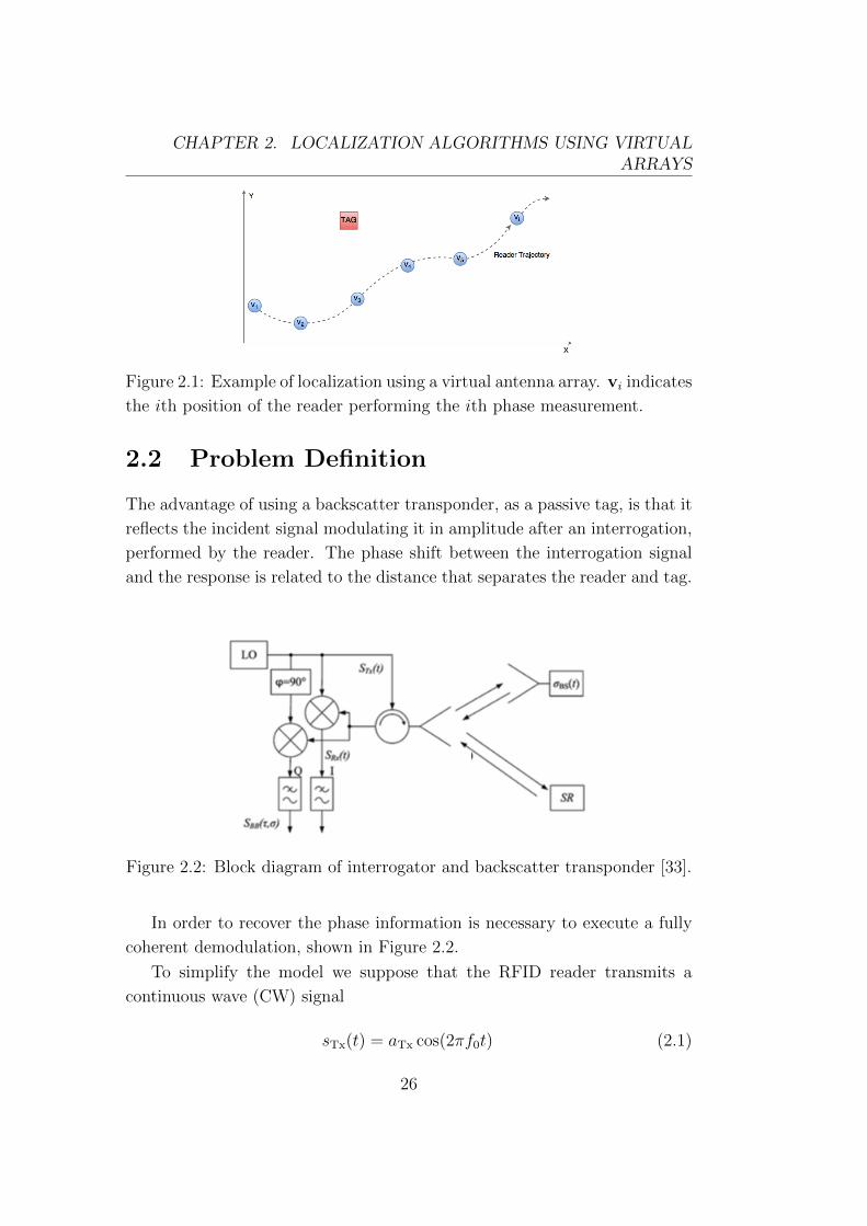
Figure 2.1: Example of localization using a virtual antenna array. vi indicates
the ith position of the reader performing the ith phase measurement.
2.2 Problem Definition
The advantage of using a backscatter transponder, as a passive tag, is that it
reflects the incident signal modulating it in amplitude after an interrogation,
performed by the reader. The phase shift between the interrogation signal
and the response is related to the distance that separates the reader and tag.
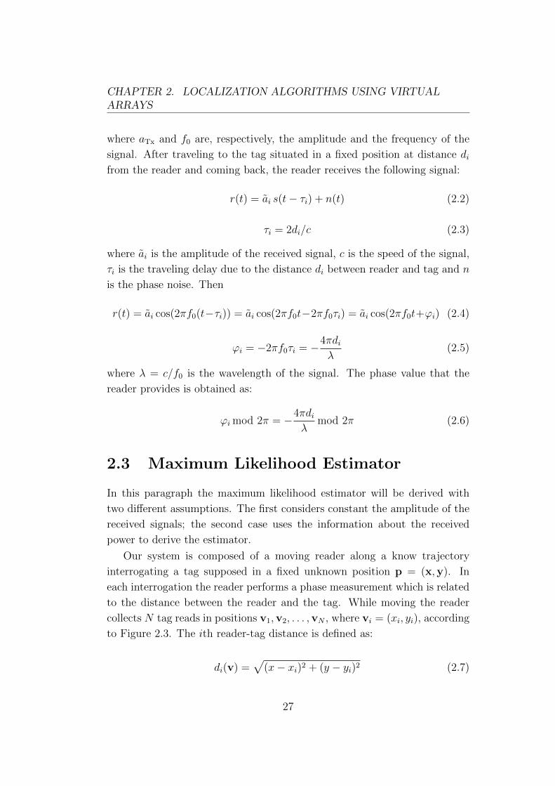
Figure 2.2: Block diagram of interrogator and backscatter transponder [33].
In order to recover the phase information is necessary to execute a fully
coherent demodulation, shown in Figure 2.2.
To simplify the model we suppose that the RFID reader transmits a
continuous wave (CW) signal
sTx(t) = aTx cos(2πf0t) (2.1)
26
CHAPTER 2. LOCALIZATION ALGORITHMS USING VIRTUALARRAYS
where aTx and f0 are, respectively, the amplitude and the frequency of the
signal. After traveling to the tag situated in a fixed position at distance difrom the reader and coming back, the reader receives the following signal:
r(t) = ai s(t− τi) + n(t) (2.2)
τi = 2di/c (2.3)
where ai is the amplitude of the received signal, c is the speed of the signal,
τi is the traveling delay due to the distance di between reader and tag and n
is the phase noise. Then
r(t) = ai cos(2πf0(t−τi)) = ai cos(2πf0t−2πf0τi) = ai cos(2πf0t+ϕi) (2.4)
ϕi = −2πf0τi = −4πdiλ
(2.5)
where λ = c/f0 is the wavelength of the signal. The phase value that the
reader provides is obtained as:
ϕi mod 2π = −4πdiλ
mod 2π (2.6)
2.3 Maximum Likelihood Estimator
In this paragraph the maximum likelihood estimator will be derived with
two different assumptions. The first considers constant the amplitude of the
received signals; the second case uses the information about the received
power to derive the estimator.
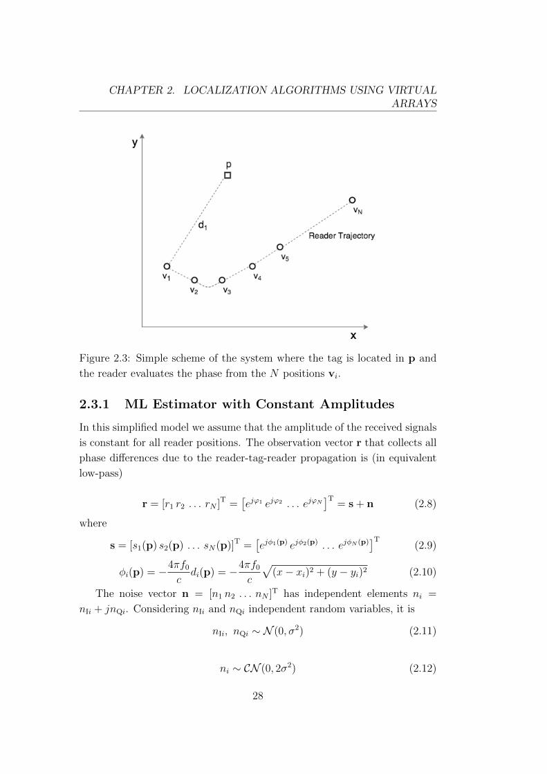
Our system is composed of a moving reader along a know trajectory
interrogating a tag supposed in a fixed unknown position p = (x,y). In
each interrogation the reader performs a phase measurement which is related
to the distance between the reader and the tag. While moving the reader
collects N tag reads in positions v1,v2, . . . ,vN , where vi = (xi, yi), according
to Figure 2.3. The ith reader-tag distance is defined as:
di(v) =√
(x− xi)2 + (y − yi)2 (2.7)
27
CHAPTER 2. LOCALIZATION ALGORITHMS USING VIRTUALARRAYS
Figure 2.3: Simple scheme of the system where the tag is located in p and
the reader evaluates the phase from the N positions vi.
2.3.1 ML Estimator with Constant Amplitudes
In this simplified model we assume that the amplitude of the received signals
is constant for all reader positions. The observation vector r that collects all
phase differences due to the reader-tag-reader propagation is (in equivalent
low-pass)
r = [r1 r2 . . . rN ]T =[ejϕ1 ejϕ2 . . . ejϕN
]T= s + n (2.8)
where
s = [s1(p) s2(p) . . . sN(p)]T =[ejφ1(p) ejφ2(p) . . . ejφN (p)
]T(2.9)
φi(p) = −4πf0c
di(p) = −4πf0c
√(x− xi)2 + (y − yi)2 (2.10)
The noise vector n = [n1 n2 . . . nN ]T has independent elements ni =
nIi + jnQi. Considering nIi and nQi independent random variables, it is
nIi, nQi ∼ N (0, σ2) (2.11)
ni ∼ CN (0, 2σ2) (2.12)
28
CHAPTER 2. LOCALIZATION ALGORITHMS USING VIRTUALARRAYS
which is a circular Gaussian random variable.
The likelihood function of the ith observation given p is
f(ri|p) =1√
2πσ2exp
{−|ri − si(p)|2
2σ2
}(2.13)
so then
f(r|p) =N∏i=1
f(ri|p) =1(√
2πσ2)N N∏
i=1
exp
{−|ri − si(p)|2
2σ2
}
=1(√
2πσ2)N exp
{− 1
2σ2
N∑i=1
|ri − si(p)|2}. (2.14)
Then, the maximum likelihood estimate p of the tag position p is
p = argmaxp
ln f(r|p) =
= argmaxp
{−
N∑i=1
|ri − si(p)|2}
=
= argmaxp
−N∑i=1
|ri|2︸ ︷︷ ︸N
−N∑i=1
|si(p)|2︸ ︷︷ ︸N
+2N∑i=1
<{ris∗i (p)}
= argmax
p
N∑i=1
<{ej(ϕi−φi(p))
}= argmax
p
N∑i=1
cos(ϕi − φi(p)) . (2.15)
Note that, according to (2.15), all the N phase measurements have the same
weight in the formula. This derives from the assumption that we considered
received signals with constant amplitude, so it is equivalent to consider the
same signal-to-noise ratio (SNR) for all the N phase measurements.
2.3.2 ML Estimator with Variable Amplitudes
In this second case we consider a model more similar to the reality. Here
each phase value measured is related to the received power at the position
from witch it was taken. So the model of the system shown in 2.8 changes
into:
29
CHAPTER 2. LOCALIZATION ALGORITHMS USING VIRTUALARRAYS
r = [r1 r2 . . . rN ]T =[a1e
jϕ1 a2ejϕ2 . . . aNe
jϕN]T
= s + n (2.16)
where
s = [s1(p, a1) s2(p, a2) . . . sN(p, aN)]T =[a1e
jφ1(p) a2ejφ2(p) . . . aNe
jφN (p)]T
(2.17)
The amplitude value ai related to the i-th reader positions is considered
as deterministic unknown parameter, not correlated to the tag position p
because the RSS is not a good position-related parameter. The amplitude
ai represents the square root of the received power reported by the reader in
the ith measurement.
The likelihood function of the ith observation given p and ai in this model
can be written as:
f(ri|p, ai) =1√
2πσ2exp
{−|ri − si(p, ai)|
2
2σ2
}
=1√
2πσ2exp
{−|ri|
2 + |si(p, ai)|2 − 2<{ris∗i (p, ai)}2σ2
}=
1√2πσ2
exp
{− a
2i + a2i − 2aiai cos(ϕi − φi(p))
2σ2
}. (2.18)
It is possible to determine the likelihood function independent of ai using
an estimate ai of ai into (2.18), which becomes
f(ri|p) = f(ri|p, ai = ai) . (2.19)
Using the maximum likelihood (ML) criterion the estimated ai is
ai = argmaxai
ln f(r|p, ai) = argmaxai
{−a2i + 2aiai cos (ϕi − φi(p))} . (2.20)
According to
ai = ai :∂
∂aif(ri|p, ai) = 0 (2.21)
we obtaine
30
CHAPTER 2. LOCALIZATION ALGORITHMS USING VIRTUALARRAYS
ai = ai cos (ϕi − φi(p)) (2.22)
and the likelihood function of the ith observation becomes
f(ri|p) =1√
2πσ2exp
{− a
2i − a2i cos2(ϕi − φi(p))
2σ2
}. (2.23)
Finally, the maximum likelihood estimate p of the tag position p is
p = argmaxp
ln f(r|p) = argmaxp
N∑i=1
a2i cos2(ϕi − φi(p)) . (2.24)
where a2i is the received power of the signal given by the reader. In this maxi-
mum likelihood estimator the phase values received with a higher power have
a greater impact on the function and on the position estimation. Comparing
(2.24) to (2.15) we note that in (2.24) more reliable phase measurements
(higher a2i ) have a higher weight in the localization process with respect to
(2.15).
2.4 Holographic Localization Method
In literature another algorithm is present, called holographic localization
method [33]. The principle is the same as previous approach i.e., the relation-
ship between phase values, antenna position and target position is unique if
a sufficient number of measurements was taken. This means that a set of N
phase measurements and a known reader trajectory identify only one possible
tag position.
According to this method the algorithm makes K hypothesis, where K �N , representing K different possible tag’s position. For each hypothesis
with coordinates (xi,yi) it calculates the distance between it and the position
where the reader takes the phase measures (xm, ym). Through the value of
the distance it derives the phase vector containing the phase values that
can be read in the N measurement positions of the reader if it will be the
correct coordinates of the tag. For each hypothesis phase vector the algorithm
31
CHAPTER 2. LOCALIZATION ALGORITHMS USING VIRTUALARRAYS
computes a sort of correlation with the phase measurements vector by:
P (p) =
∣∣∣∣ N∑m=1
amej(
4πdm,iλc
−ϕm)∣∣∣∣= ∣∣∣∣ N∑
m=1
amej(−φm−ϕm)
∣∣∣∣ (2.25)
where P (p) is the correlation function, dm,i is the distance between the cur-
rent hypothesis and the antenna position m, am is the amplitude measured
at the antenna position m, λc is the carrier wavelength and ϕm is the phase
measured at the antenna position m. The hypothesis that maximizes the
function (2.25) is the detected position of the tag.
This method is very similar to approaches that calculate the AOA from
phase difference of arrival from different positions and calculate the triangu-
lation to find the tag position [34]. This formula is not the rigorous maximum
likelihood estimator, but at high SNR where the phase estimation errors are
small, holographic localization performance should be very similar to ML
derived in (2.24). In fact,
p = argmaxp
∣∣∣∣∣N∑m=1
amej(−φm(p)−ϕm)
∣∣∣∣∣ =
= argmaxp
√√√√( N∑m=1
am cos(−φm(p)− ϕm)
)2
+
(N∑m=1
am sin(−φm(p)− ϕm)
)2
= argmaxp
am
√√√√( N∑m=1
cos(−φm(p)− ϕm)
)2
+
(N∑m=1
sin(−φm(p)− ϕm)
)2
(2.26)
At high SNR, sin(−φm(p)− ϕm) ≈ 0 so
p ≈ argmaxp
(am(cos(−φm(p)− ϕm))2
)(2.27)
where am is the power received at the m-th antenna positions, ϕm is the
phase measured at the m-th antenna positions and φm(p) is the theoretical
phase.
32

Chapter 3
Simulation Results
In this chapter the performance of the localization system are reported through
Matlab simulations.
The algorithm used in the simulations is explained in Sec. 2.4.
3.1 Monodimensional Algorithm
For simulating this system in Matlab we made a series of assumptions in
order to decrease the computational complexity and understand how several
features of the environment and the technology can impact the performance.
The assumptions are:
• the tag is fix in a position with coordinates p = (x, y);
• the reader is moving along a linear trajectory with constant speed;
• the distance between the tag and the reader’s trajectory (y) is known,
so it transforms the problem in monodimensional localization where
the only unknown variable is the longitudinal coordinate (x).
These hypotheses permit to have a faster simulation and a lower complexity
than the 2D case [33]. The complexity becomes:
Ncalculation ∼ KNantennas (3.1)
where K is the number of hypothesis along the x-coordinate and Nantennas
are the number of phase measures that the reader took. In the following
33
CHAPTER 3. SIMULATION RESULTS
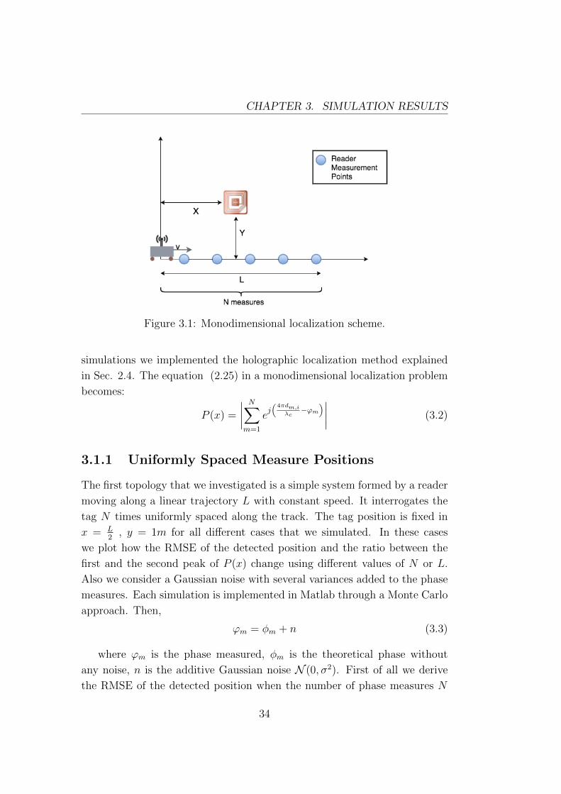
Figure 3.1: Monodimensional localization scheme.
simulations we implemented the holographic localization method explained
in Sec. 2.4. The equation (2.25) in a monodimensional localization problem
becomes:
P (x) =
∣∣∣∣ N∑m=1
ej(
4πdm,iλc
−ϕm)∣∣∣∣ (3.2)
3.1.1 Uniformly Spaced Measure Positions
The first topology that we investigated is a simple system formed by a reader
moving along a linear trajectory L with constant speed. It interrogates the
tag N times uniformly spaced along the track. The tag position is fixed in
x = L2
, y = 1m for all different cases that we simulated. In these cases
we plot how the RMSE of the detected position and the ratio between the
first and the second peak of P (x) change using different values of N or L.
Also we consider a Gaussian noise with several variances added to the phase
measures. Each simulation is implemented in Matlab through a Monte Carlo
approach. Then,
ϕm = φm + n (3.3)
where ϕm is the phase measured, φm is the theoretical phase without
any noise, n is the additive Gaussian noise N (0, σ2). First of all we derive
the RMSE of the detected position when the number of phase measures N
34
CHAPTER 3. SIMULATION RESULTS
1 2 3 4 5 6 7 8 9 100
0.5
1
1.5
2
2.5
3
3.5
4
4.5
5
N
RM
SE
[m
]
σ =0.032
σ =0.1
σ =0.32
σ =0.707
σ =1
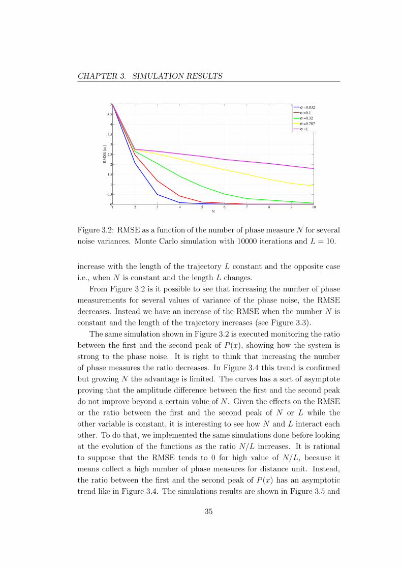
Figure 3.2: RMSE as a function of the number of phase measure N for several
noise variances. Monte Carlo simulation with 10000 iterations and L = 10.
increase with the length of the trajectory L constant and the opposite case
i.e., when N is constant and the length L changes.
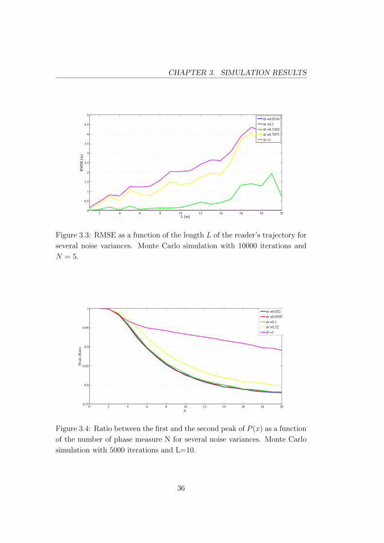
From Figure 3.2 is it possible to see that increasing the number of phase
measurements for several values of variance of the phase noise, the RMSE
decreases. Instead we have an increase of the RMSE when the number N is
constant and the length of the trajectory increases (see Figure 3.3).
The same simulation shown in Figure 3.2 is executed monitoring the ratio
between the first and the second peak of P (x), showing how the system is
strong to the phase noise. It is right to think that increasing the number
of phase measures the ratio decreases. In Figure 3.4 this trend is confirmed
but growing N the advantage is limited. The curves has a sort of asymptote
proving that the amplitude difference between the first and the second peak
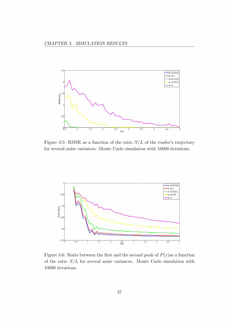
do not improve beyond a certain value of N . Given the effects on the RMSE
or the ratio between the first and the second peak of N or L while the
other variable is constant, it is interesting to see how N and L interact each
other. To do that, we implemented the same simulations done before looking
at the evolution of the functions as the ratio N/L increases. It is rational
to suppose that the RMSE tends to 0 for high value of N/L, because it
means collect a high number of phase measures for distance unit. Instead,
the ratio between the first and the second peak of P (x) has an asymptotic
trend like in Figure 3.4. The simulations results are shown in Figure 3.5 and
35
CHAPTER 3. SIMULATION RESULTS
2 4 6 8 10 12 14 16 18 200
0.5
1
1.5
2
2.5
3
3.5
4
4.5
5
L [m]
RM
SE
[m
]
σ =0.0316
σ =0.1
σ =0.3162
σ =0.7071
σ =1
Figure 3.3: RMSE as a function of the length L of the reader’s trajectory for
several noise variances. Monte Carlo simulation with 10000 iterations and
N = 5.
0 2 4 6 8 10 12 14 16 18 200.75
0.8
0.85
0.9
0.95
1
N
Peaks R
ati
o
σ =0.032
σ =0.0707
σ =0.1
σ =0.32
σ =1
Figure 3.4: Ratio between the first and the second peak of P (x) as a function
of the number of phase measure N for several noise variances. Monte Carlo
simulation with 5000 iterations and L=10.
36
CHAPTER 3. SIMULATION RESULTS
0.5 1 1.5 2 2.5 3 3.5 4 4.5 50
0.5
1
1.5
2
2.5
N/L
RM
SE
[m
]
σ =0.0316
σ =0.1
σ =0.3162
σ =0.7071
σ =1
Figure 3.5: RMSE as a function of the ratio N/L of the reader’s trajectory
for several noise variances. Monte Carlo simulation with 10000 iterations.
0 0.5 1 1.5 2 2.5 3 3.5 4 4.5 50.75
0.8
0.85
0.9
0.95
1
N/L
Peaks R
ati
o
σ =0.03162
σ =0.1
σ =0.3162
σ =0.707
σ =1
Figure 3.6: Ratio between the first and the second peak of P (x)as a function
of the ratio N/L for several noise variances. Monte Carlo simulation with
10000 iterations.
37
CHAPTER 3. SIMULATION RESULTS
0 0.1 0.2 0.3 0.4 0.5 0.6 0.7 0.8 0.9 10
0.2
0.4
0.6
0.8
1
1.2
1.4
1.6
σ2
RM
SE
[m
]
N/L=4/4
N/L=6/6
N/L=10/10
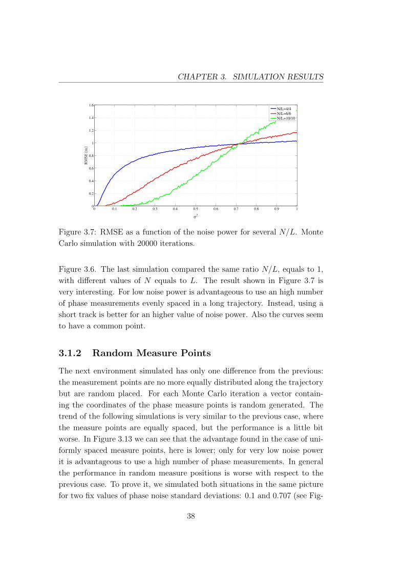
Figure 3.7: RMSE as a function of the noise power for several N/L. Monte
Carlo simulation with 20000 iterations.
Figure 3.6. The last simulation compared the same ratio N/L, equals to 1,
with different values of N equals to L. The result shown in Figure 3.7 is
very interesting. For low noise power is advantageous to use an high number
of phase measurements evenly spaced in a long trajectory. Instead, using a
short track is better for an higher value of noise power. Also the curves seem
to have a common point.
3.1.2 Random Measure Points
The next environment simulated has only one difference from the previous:
the measurement points are no more equally distributed along the trajectory
but are random placed. For each Monte Carlo iteration a vector contain-
ing the coordinates of the phase measure points is random generated. The
trend of the following simulations is very similar to the previous case, where
the measure points are equally spaced, but the performance is a little bit
worse. In Figure 3.13 we can see that the advantage found in the case of uni-
formly spaced measure points, here is lower; only for very low noise power
it is advantageous to use a high number of phase measurements. In general
the performance in random measure positions is worse with respect to the
previous case. To prove it, we simulated both situations in the same picture
for two fix values of phase noise standard deviations: 0.1 and 0.707 (see Fig-
38
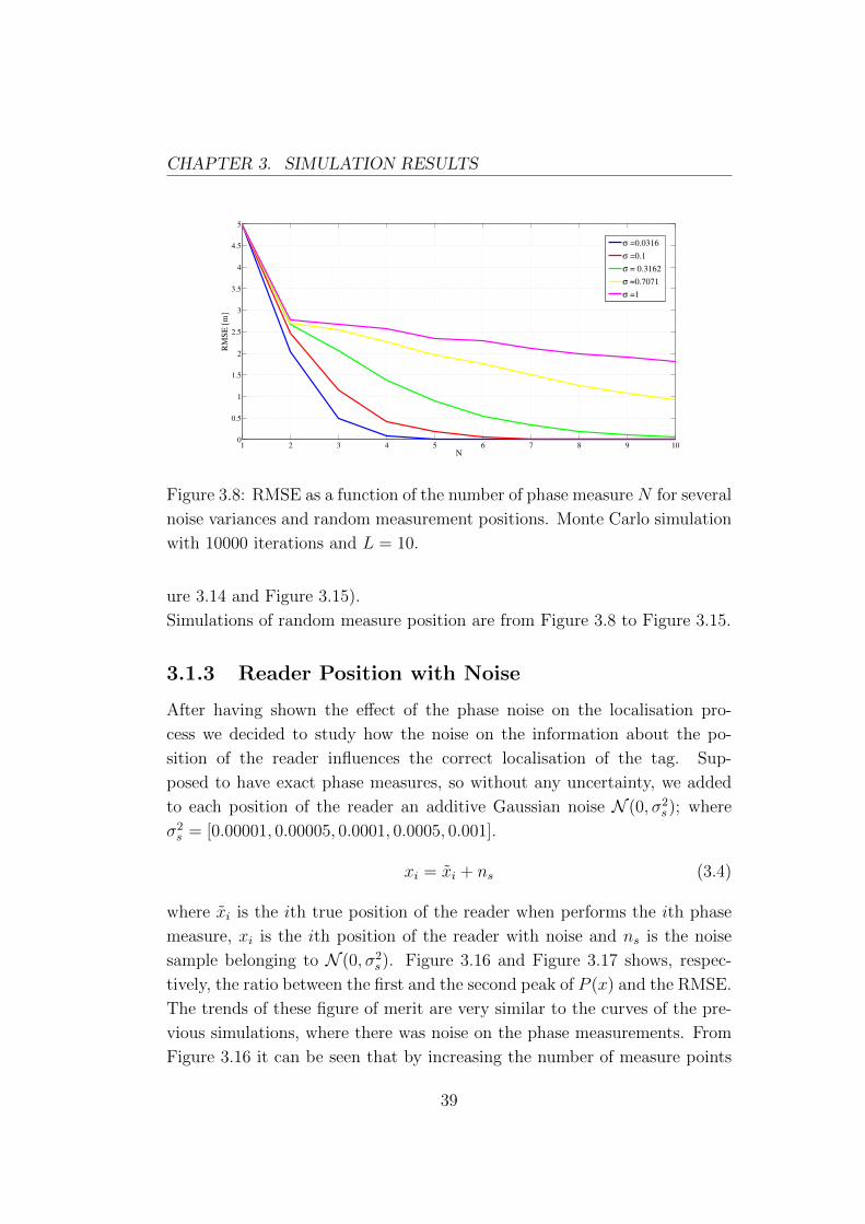
CHAPTER 3. SIMULATION RESULTS
1 2 3 4 5 6 7 8 9 100
0.5
1
1.5
2
2.5
3
3.5
4
4.5
5
N
RM
SE
[m
]
σ =0.0316
σ =0.1
σ = 0.3162
σ =0.7071
σ =1
Figure 3.8: RMSE as a function of the number of phase measure N for several
noise variances and random measurement positions. Monte Carlo simulation
with 10000 iterations and L = 10.
ure 3.14 and Figure 3.15).
Simulations of random measure position are from Figure 3.8 to Figure 3.15.
3.1.3 Reader Position with Noise
After having shown the effect of the phase noise on the localisation pro-
cess we decided to study how the noise on the information about the po-
sition of the reader influences the correct localisation of the tag. Sup-
posed to have exact phase measures, so without any uncertainty, we added
to each position of the reader an additive Gaussian noise N (0, σ2s); where
σ2s = [0.00001, 0.00005, 0.0001, 0.0005, 0.001].
xi = xi + ns (3.4)
where xi is the ith true position of the reader when performs the ith phase
measure, xi is the ith position of the reader with noise and ns is the noise
sample belonging to N (0, σ2s). Figure 3.16 and Figure 3.17 shows, respec-
tively, the ratio between the first and the second peak of P (x) and the RMSE.
The trends of these figure of merit are very similar to the curves of the pre-
vious simulations, where there was noise on the phase measurements. From
Figure 3.16 it can be seen that by increasing the number of measure points
39
CHAPTER 3. SIMULATION RESULTS
0 2 4 6 8 10 12 14 16 18 200
10
20
30
40
50
60
70
80
L [m]
RM
SE
[m
]
σ =0.03162
σ =0.1
σ =0.3162
σ =0.707
σ =1
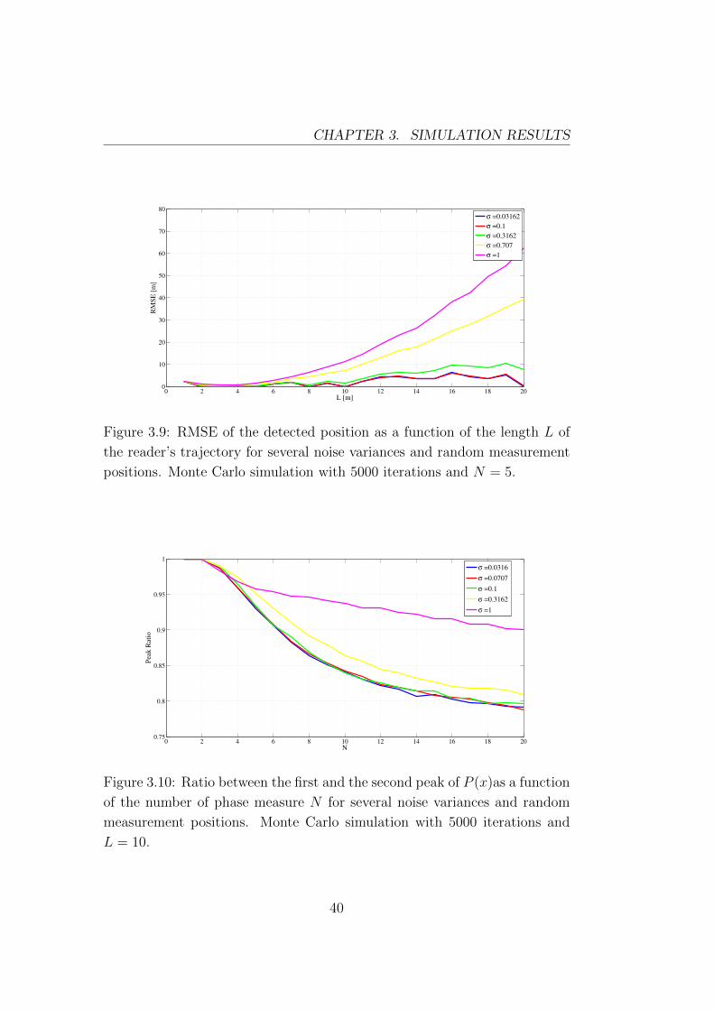
Figure 3.9: RMSE of the detected position as a function of the length L of
the reader’s trajectory for several noise variances and random measurement
positions. Monte Carlo simulation with 5000 iterations and N = 5.
0 2 4 6 8 10 12 14 16 18 200.75
0.8
0.85
0.9
0.95
1
N
Peak R
ati
o
σ =0.0316
σ =0.0707
σ =0.1
σ =0.3162
σ =1
Figure 3.10: Ratio between the first and the second peak of P (x)as a function
of the number of phase measure N for several noise variances and random
measurement positions. Monte Carlo simulation with 5000 iterations and
L = 10.
40
CHAPTER 3. SIMULATION RESULTS
0.5 1 1.5 2 2.5 3 3.5 4 4.5 50
0.5
1
1.5
2
2.5
N/L
RM
SE
[m
]
σ =0.0316
σ =0.1
σ = 0.3162
σ =0.7071
σ =1
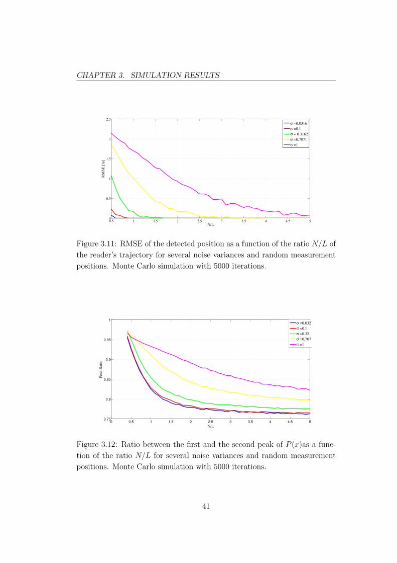
Figure 3.11: RMSE of the detected position as a function of the ratio N/L of
the reader’s trajectory for several noise variances and random measurement
positions. Monte Carlo simulation with 5000 iterations.
0 0.5 1 1.5 2 2.5 3 3.5 4 4.5 50.75
0.8
0.85
0.9
0.95
1
N/L
Peak R
ati
o
σ =0.032
σ =0.1
σ =0.32
σ =0.707
σ =1
Figure 3.12: Ratio between the first and the second peak of P (x)as a func-
tion of the ratio N/L for several noise variances and random measurement
positions. Monte Carlo simulation with 5000 iterations.
41
CHAPTER 3. SIMULATION RESULTS
0 0.1 0.2 0.3 0.4 0.5 0.6 0.7 0.8 0.9 10
0.2
0.4
0.6
0.8
1
1.2
1.4
1.6
1.8
2
σ2
RM
SE
[m
]
N/L=4/4
N/L=6/6
N/L=10/10
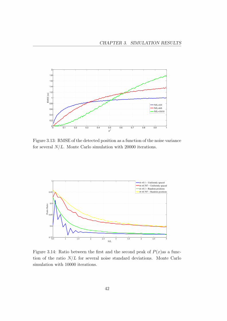
Figure 3.13: RMSE of the detected position as a function of the noise variance
for several N/L. Monte Carlo simulation with 20000 iterations.
0.5 1 1.5 2 2.5 3 3.5 4 4.5 50.75
0.8
0.85
0.9
0.95
1
N/L
Pea
ks
Rat
io
σ =0.1 − Uniformly spaced
σ =0.707 − Uniformly spaced
σ =0.1 − Random positions
σ =0.707 − Random positions
Figure 3.14: Ratio between the first and the second peak of P (x)as a func-
tion of the ratio N/L for several noise standard deviations. Monte Carlo
simulation with 10000 iterations.
42
CHAPTER 3. SIMULATION RESULTS
0.5 1 1.5 2 2.5 3 3.5 4 4.5 50
0.2
0.4
0.6
0.8
1
1.2
1.4
1.6
1.8
2
N/L
RM
SE
[m
]
σ =0.1 − Uniformly spaced
σ =0.707 − Uniformly spaced
σ =0.1 − Random positions
σ =0.707 − Random positions
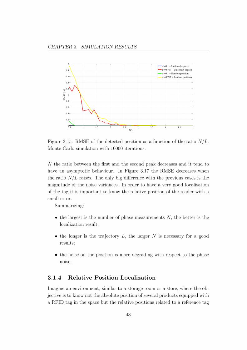
Figure 3.15: RMSE of the detected position as a function of the ratio N/L.
Monte Carlo simulation with 10000 iterations.
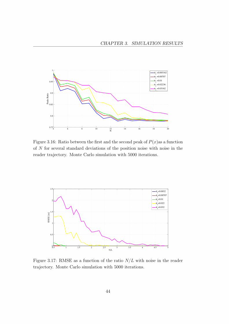
N the ratio between the first and the second peak decreases and it tend to
have an asymptotic behaviour. In Figure 3.17 the RMSE decreases when
the ratio N/L raises. The only big difference with the previous cases is the
magnitude of the noise variances. In order to have a very good localisation
of the tag it is important to know the relative position of the reader with a
small error.
Summarizing:
• the largest is the number of phase measurements N , the better is the
localization result;
• the longer is the trajectory L, the larger N is necessary for a good
results;
• the noise on the position is more degrading with respect to the phase
noise.
3.1.4 Relative Position Localization
Imagine an environment, similar to a storage room or a store, where the ob-
jective is to know not the absolute position of several products equipped with
a RFID tag in the space but the relative positions related to a reference tag
43
CHAPTER 3. SIMULATION RESULTS
4 6 8 10 12 14 16 18 200.75
0.8
0.85
0.9
0.95
1
N
Peaks R
ati
o
σs =0.003162
σs =0.00707
σs =0.01
σs =0.02236
σs =0.03162
Figure 3.16: Ratio between the first and the second peak of P (x)as a function
of N for several standard deviations of the position noise with noise in the
reader trajectory. Monte Carlo simulation with 5000 iterations.
0.5 1 1.5 2 2.5 3 3.5 4 4.5 50
0.5
1
1.5
2
2.5
N/L
RM
SE
[m
]
σs=0.0032
σs=0.00707
σs=0.01
σs=0.022
σs=0.032
Figure 3.17: RMSE as a function of the ratio N/L with noise in the reader
trajectory. Monte Carlo simulation with 5000 iterations.
44
CHAPTER 3. SIMULATION RESULTS
with known location. This tag can be positioned on a shelving or in other
place. It has been found that, if the reader position errors are independent,
locating the reference tag and the tag with unknown position separately, us-
ing the algorithm explained before, and then derive the unknown tag position
through the error on the first device is not useful. Supposing that the mov-
ing reader is equipped with high precision odometers or something similar,
it is correct to think that the position error between consecutive locations
is negligible for a small trajectory. Only on the starting point of the track
a significant error is present. In the simulation program we added the same
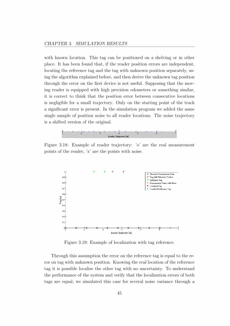
single sample of position noise to all reader locations. The noise trajectory
is a shifted version of the original.
Figure 3.18: Example of reader trajectory: ’o’ are the real measurement
points of the reader, ’x’ are the points with noise.
Figure 3.19: Example of localization with tag reference.
Through this assumption the error on the reference tag is equal to the er-
ror on tag with unknown position. Knowing the real location of the reference
tag it is possible localize the other tag with no uncertainty. To understand
the performance of the system and verify that the localization errors of both
tags are equal, we simulated this case for several noise variance through a
45
CHAPTER 3. SIMULATION RESULTS
Monte Carlo simulation where we counted the number of times that localiza-
tion errors were different each other. The result is an empty histogram for all
variance used. This means, under the assumption done before, that always
the error on the localized position of the reference tag is equal to the error of
the other device with unknown position; so the latter can be localized with
precision.
3.1.5 Not Central Tag Position
In previous simulations a strong assumption was that the x-coordinate of the
tag was positioned in the middle of the trajectory. The geometry of the sys-
tem influences the locating process result, so we decided to investigate about
the impact of the relative tag position with respect to the reader trajectory.
To do that we implemented a simulation where the tag is located in a fixed
position and the linear trajectory, with length fixed to L, is moved adding
an offset factor, called ∆. When ∆ is equal to 0 means that the trajectory
is centered with respect to the tag i.e., reader measurement positions are
between −L2
and L2. Adding or subtracting a ∆ factor to all reader measure
positions means move the reader trajectory on the right or on the left with
respect to the tag location. For each value of ∆ factor we calculated the
RMSE using the same position noise samples.
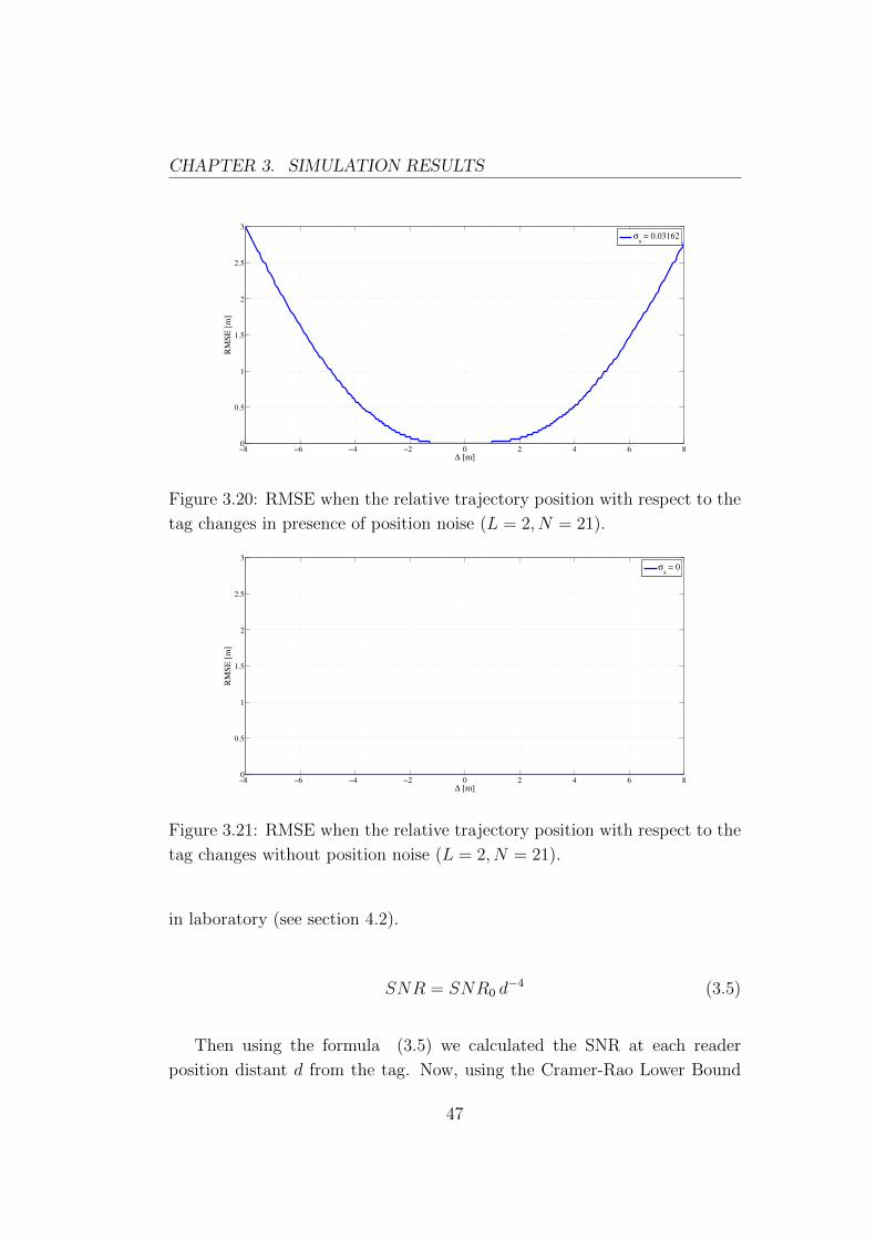
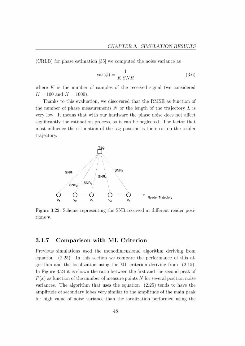
Looking at Figure 3.20, it is possible see that the RMSE modifies its value
as the ∆ factor changes. In particular the RMSE has zero value when the
trajectory is opposite to the tag position and it increases when the trajectory
moves from it. Figure 3.21 shows the same simulation but without position
noise; in this situation the position of the trajectory with respect to the tag
does not influence the localization process result.
3.1.6 Signal-to-Noise Ratio Simulation
The previous simulations considered the phase noise independently to the
SNR at the considered reader position. In the following simulation we decided
to test the algorithm generating the noise samples with variance according
to the effective reader position.
First of all we have extrapolated experimentally the signal to noise ratio
at the distance of 1 meter (SNR0) using the real hardware setup available
46
CHAPTER 3. SIMULATION RESULTS
−8 −6 −4 −2 0 2 4 6 80
0.5
1
1.5
2
2.5
3
∆ [m]
RM
SE
[m
]
σs = 0.03162
Figure 3.20: RMSE when the relative trajectory position with respect to the
tag changes in presence of position noise (L = 2, N = 21).
−8 −6 −4 −2 0 2 4 6 80
0.5
1
1.5
2
2.5
3
∆ [m]
RM
SE
[m
]
σs = 0
Figure 3.21: RMSE when the relative trajectory position with respect to the
tag changes without position noise (L = 2, N = 21).
in laboratory (see section 4.2).
SNR = SNR0 d−4 (3.5)
Then using the formula (3.5) we calculated the SNR at each reader
position distant d from the tag. Now, using the Cramer-Rao Lower Bound
47
CHAPTER 3. SIMULATION RESULTS
(CRLB) for phase estimation [35] we computed the noise variance as
var(ϕ) =1
K SNR(3.6)
where K is the number of samples of the received signal (we considered
K = 100 and K = 1000).
Thanks to this evaluation, we discovered that the RMSE as function of
the number of phase measurements N or the length of the trajectory L is
very low. It means that with our hardware the phase noise does not affect
significantly the estimation process, so it can be neglected. The factor that
most influence the estimation of the tag position is the error on the reader
trajectory.
Figure 3.22: Scheme representing the SNR received at different reader posi-
tions v.
3.1.7 Comparison with ML Criterion
Previous simulations used the monodimensional algorithm deriving from
equation (2.25). In this section we compare the performance of this al-
gorithm and the localization using the ML criterion deriving from (2.15).
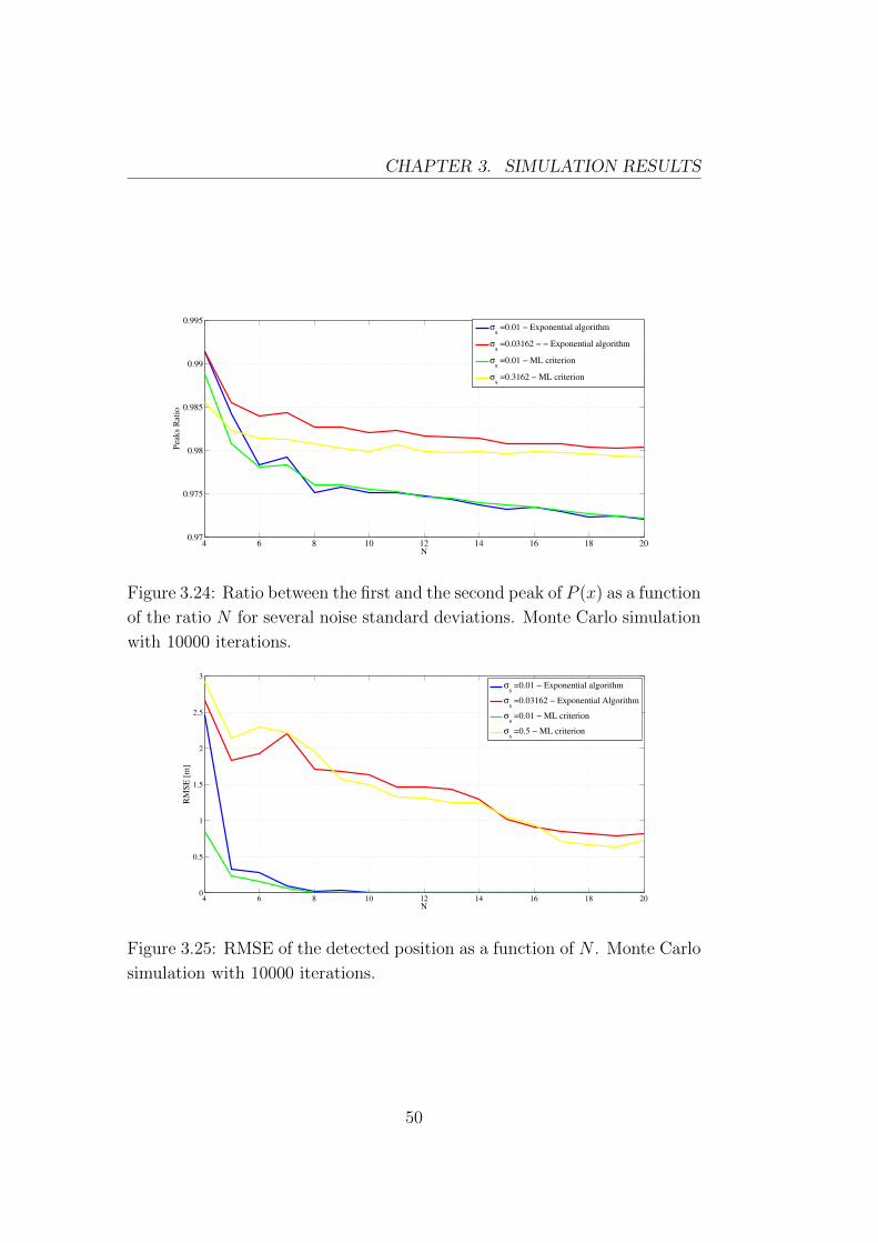
In Figure 3.24 it is shown the ratio between the first and the second peak of
P (x) as function of the number of measure points N for several position noise
variances. The algorithm that uses the equation (2.25) tends to have the
amplitude of secondary lobes very similar to the amplitude of the main peak
for high value of noise variance than the localization performed using the
48
CHAPTER 3. SIMULATION RESULTS
ML criterion. Amplitude of secondary lobes comparable to the main peak
can create an ambiguity problem i.e., a secondary lobe can be choosen as
estimated position generating a high estimation error. A sharper main peak
indicates an estimation with a high accuracy. Using a smaller noise variance
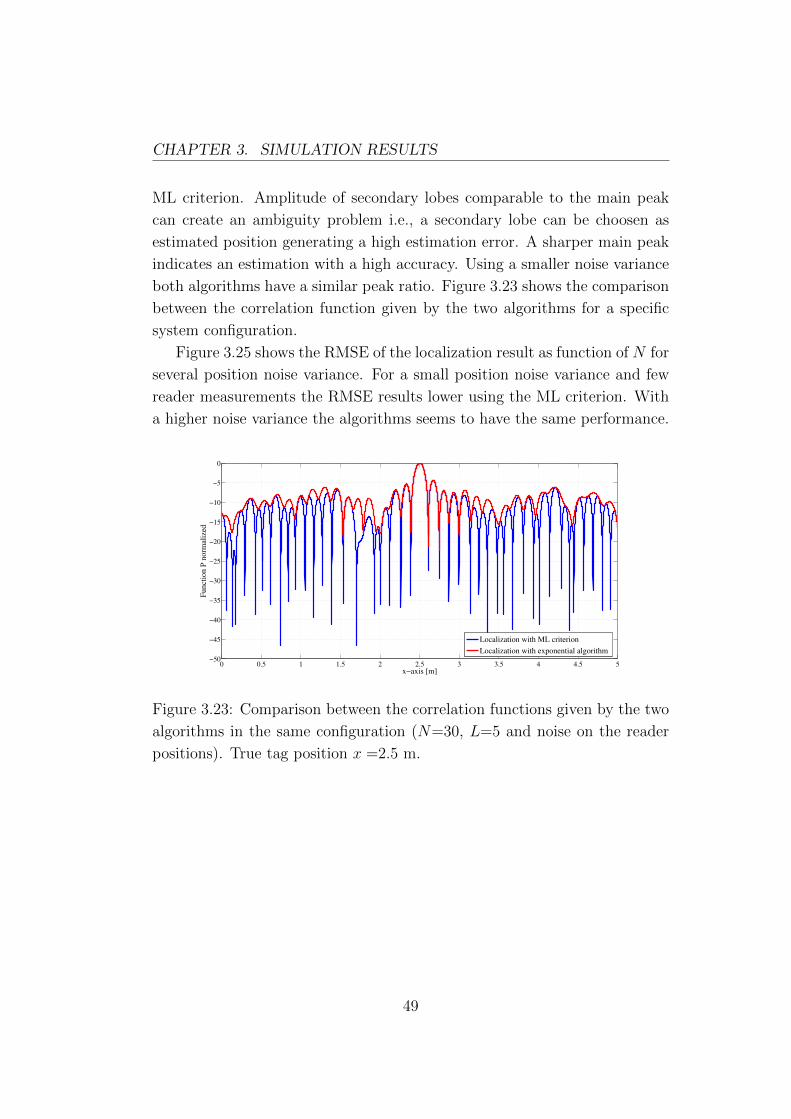
both algorithms have a similar peak ratio. Figure 3.23 shows the comparison
between the correlation function given by the two algorithms for a specific
system configuration.
Figure 3.25 shows the RMSE of the localization result as function of N for
several position noise variance. For a small position noise variance and few
reader measurements the RMSE results lower using the ML criterion. With
a higher noise variance the algorithms seems to have the same performance.
0 0.5 1 1.5 2 2.5 3 3.5 4 4.5 5−50
−45
−40
−35
−30
−25
−20
−15
−10
−5
0
x−axis [m]
Funct
ion P
norm
aliz
ed
Localization with ML criterion
Localization with exponential algorithm
Figure 3.23: Comparison between the correlation functions given by the two
algorithms in the same configuration (N=30, L=5 and noise on the reader
positions). True tag position x =2.5 m.
49
CHAPTER 3. SIMULATION RESULTS
4 6 8 10 12 14 16 18 200.97
0.975
0.98
0.985
0.99
0.995
N
Pea
ks
Rat
io
σs =0.01 − Exponential algorithm
σs =0.03162 − − Exponential algorithm
σs =0.01 − ML criterion
σs =0.3162 − ML criterion
Figure 3.24: Ratio between the first and the second peak of P (x) as a function
of the ratio N for several noise standard deviations. Monte Carlo simulation
with 10000 iterations.
4 6 8 10 12 14 16 18 200
0.5
1
1.5
2
2.5
3
N
RM
SE
[m
]
σs =0.01 − Exponential algorithm
σs =0.03162 − Exponential Algorithm
σs =0.01 − ML criterion
σs =0.5 − ML criterion
Figure 3.25: RMSE of the detected position as a function of N . Monte Carlo
simulation with 10000 iterations.
50
Chapter 4
Measurement Setup
4.1 Hardware and Software
4.1.1 Reader
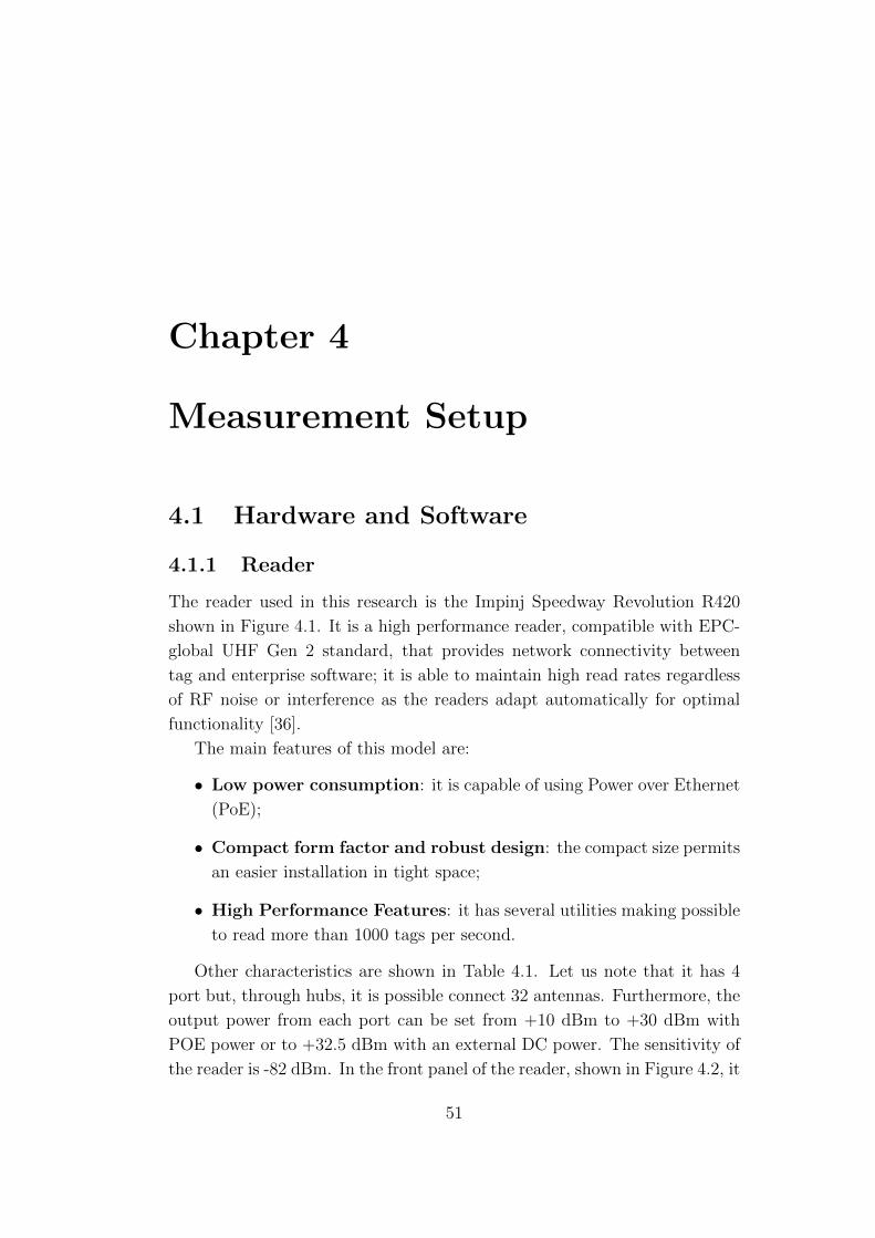
The reader used in this research is the Impinj Speedway Revolution R420
shown in Figure 4.1. It is a high performance reader, compatible with EPC-
global UHF Gen 2 standard, that provides network connectivity between
tag and enterprise software; it is able to maintain high read rates regardless
of RF noise or interference as the readers adapt automatically for optimal
functionality [36].
The main features of this model are:
• Low power consumption: it is capable of using Power over Ethernet
(PoE);
• Compact form factor and robust design: the compact size permits
an easier installation in tight space;
• High Performance Features: it has several utilities making possible
to read more than 1000 tags per second.
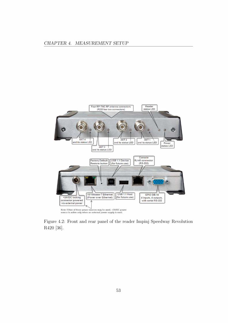
Other characteristics are shown in Table 4.1. Let us note that it has 4
port but, through hubs, it is possible connect 32 antennas. Furthermore, the
output power from each port can be set from +10 dBm to +30 dBm with
POE power or to +32.5 dBm with an external DC power. The sensitivity of
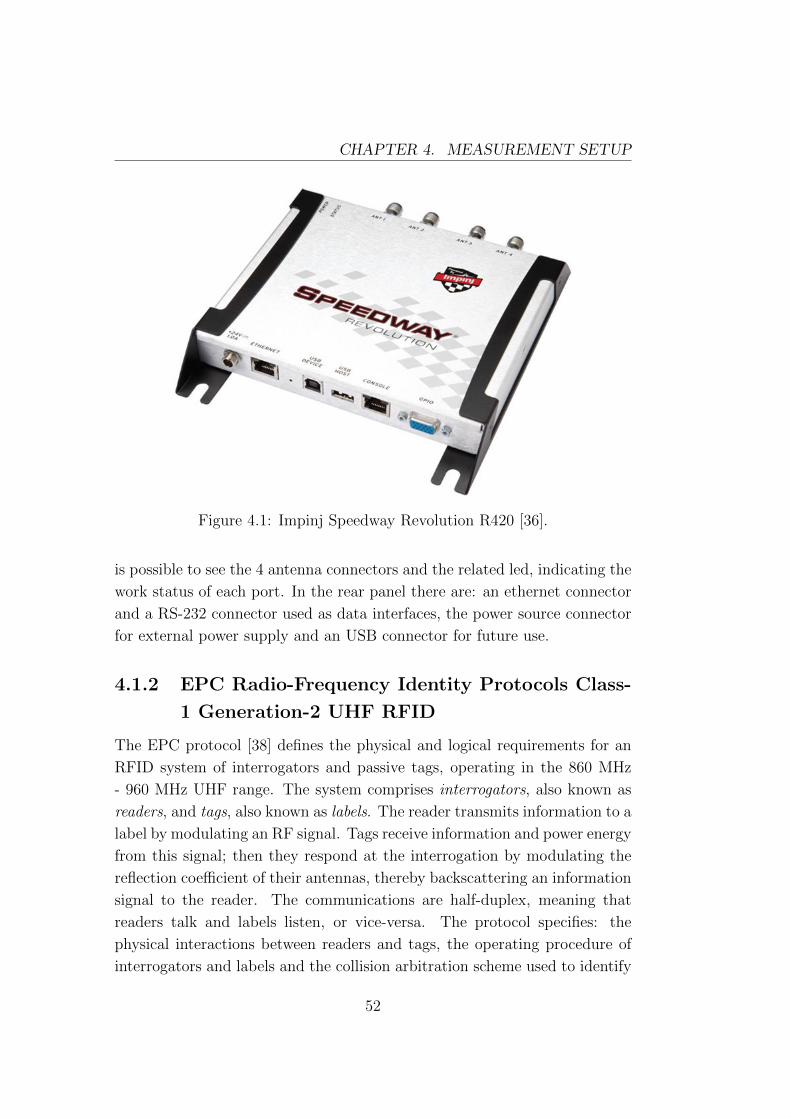
the reader is -82 dBm. In the front panel of the reader, shown in Figure 4.2, it
51
CHAPTER 4. MEASUREMENT SETUP
Figure 4.1: Impinj Speedway Revolution R420 [36].
is possible to see the 4 antenna connectors and the related led, indicating the
work status of each port. In the rear panel there are: an ethernet connector
and a RS-232 connector used as data interfaces, the power source connector
for external power supply and an USB connector for future use.
4.1.2 EPC Radio-Frequency Identity Protocols Class-
1 Generation-2 UHF RFID
The EPC protocol [38] defines the physical and logical requirements for an
RFID system of interrogators and passive tags, operating in the 860 MHz
- 960 MHz UHF range. The system comprises interrogators, also known as
readers, and tags, also known as labels. The reader transmits information to a
label by modulating an RF signal. Tags receive information and power energy
from this signal; then they respond at the interrogation by modulating the
reflection coefficient of their antennas, thereby backscattering an information
signal to the reader. The communications are half-duplex, meaning that
readers talk and labels listen, or vice-versa. The protocol specifies: the
physical interactions between readers and tags, the operating procedure of
interrogators and labels and the collision arbitration scheme used to identify
52
CHAPTER 4. MEASUREMENT SETUP
Figure 4.2: Front and rear panel of the reader Impinj Speedway Revolution
R420 [36].
53
CHAPTER 4. MEASUREMENT SETUP
Table 4.1: Main features of Impinj Speedway Revolution R420 [37].
Product Details Speedway R420
Air Interface Protocol GS1/EPCglobal UHF Gen2 (ISO 18000-6C) or RAIN RFID
Antenna Ports 4 expandable to 32 antennas with Speedway Antenna Hub
Supported Regions or
Geographies
FCC (TWYIPJREV), Canada (6324A-IPJREV), Australia,
Brazil (Anatel), China (CMIT 2010DJ4065),
EU (CE Mark, ETSI EN408 208 v1.4.1), Hong Kong,
India, Japan (920MHz band), Korea (UQC-R420),
Malaysia, New Zealand (Z233), Singapore,
South Africa (ICASA), Taiwan (CCAF10LP1290T5),
Thailand, Uruguay, UAE, Vietnam
Transmit Power+10.0 to +31.5 dBm (PoE) (EU1 limited to +30 dBm),
+10.0 to +32.5 dBm(Listed/Certified power supply)
Max Receive Sensitivity -84 dBm
Min Return Loss 10 dB
Application Interfaces
Low Level Reader Protocol (LLRP): C, C++, Java,
and C# libraries,
OctaneSDK: Java or C#,
On-reader Applications via Octane ETK: C, C++
Network Connectivity
10/100BASE-T auto-negotiate
802.1x with PEAP/TLS and MD5 support,
WPA for Wifi and Ethernet,
3rd party Wifi adapters supported via USB interface.
Speedway Connect:
HID (keyboard) emulation,
TCP Socket, Serial/RS-232, HTTP POST
Power Sources
Power over Ethernet (PoE) IEEE 802.3af,
Listed/Certified power supply
rated minimum 2.5A
Operating Temperature -20 C to +50 C
Dimensions & Weight 7.5 in H x 6.9 in W x 1.2 in D (19 x 17.5 x 3 cm)
54
CHAPTER 4. MEASUREMENT SETUP
a specific tag in a environment full of different label.
The commands described in the protocol are divided into:
• Mandatory commands: Conforming tags and readers shall support
all mandatory commands;
• Optional commands: Conforming tags or interrogators may or may
not support optional commands;
• Proprietary commands: Proprietary commands may be enabled in
conformance with this specification, but are not specified herein and
shall be capable of being permanently disabled. Proprietary commands
are intended for manufacturing purposes and shall not be used in field-
deployed RFID systems;
• Custom commands: Custom commands may be enabled in confor-
mance with this specification, but are not specified herein.
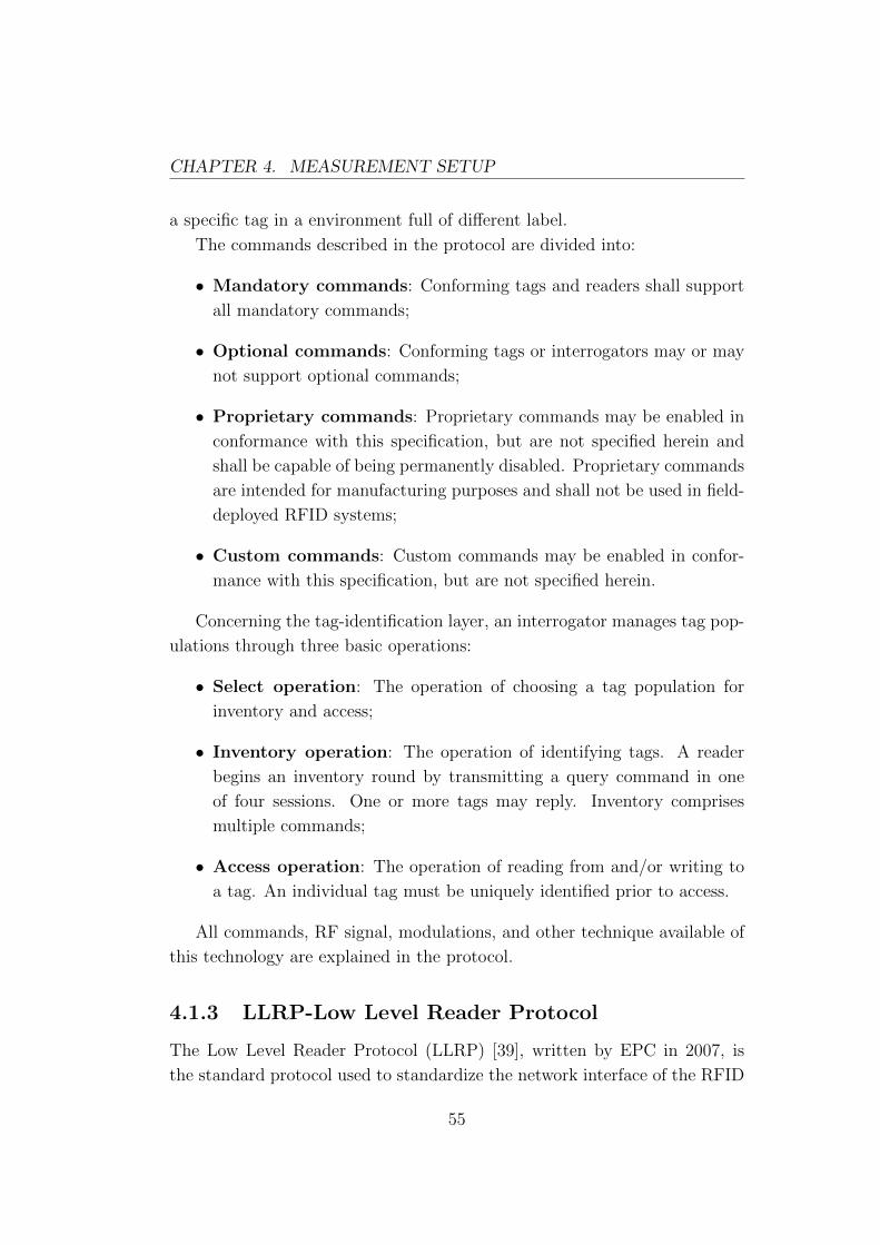
Concerning the tag-identification layer, an interrogator manages tag pop-
ulations through three basic operations:
• Select operation: The operation of choosing a tag population for
inventory and access;
• Inventory operation: The operation of identifying tags. A reader
begins an inventory round by transmitting a query command in one
of four sessions. One or more tags may reply. Inventory comprises
multiple commands;
• Access operation: The operation of reading from and/or writing to
a tag. An individual tag must be uniquely identified prior to access.
All commands, RF signal, modulations, and other technique available of
this technology are explained in the protocol.
4.1.3 LLRP-Low Level Reader Protocol
The Low Level Reader Protocol (LLRP) [39], written by EPC in 2007, is
the standard protocol used to standardize the network interface of the RFID
55
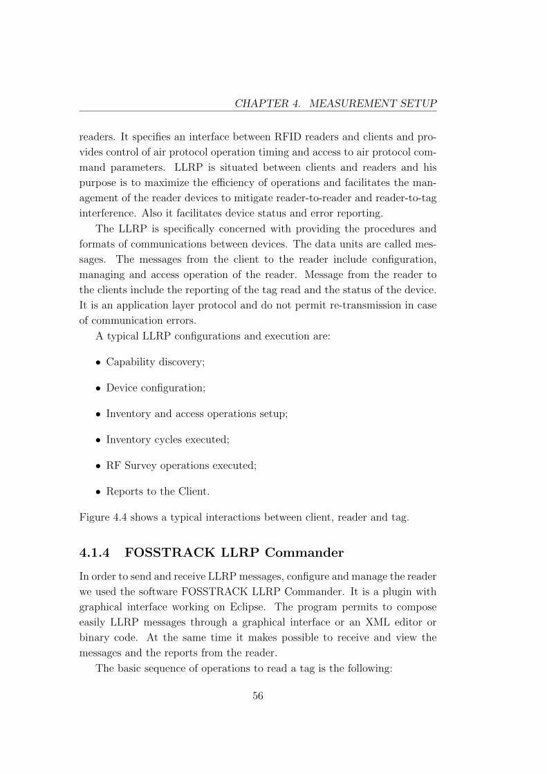
CHAPTER 4. MEASUREMENT SETUP
readers. It specifies an interface between RFID readers and clients and pro-
vides control of air protocol operation timing and access to air protocol com-
mand parameters. LLRP is situated between clients and readers and his
purpose is to maximize the efficiency of operations and facilitates the man-
agement of the reader devices to mitigate reader-to-reader and reader-to-tag
interference. Also it facilitates device status and error reporting.
The LLRP is specifically concerned with providing the procedures and
formats of communications between devices. The data units are called mes-
sages. The messages from the client to the reader include configuration,
managing and access operation of the reader. Message from the reader to
the clients include the reporting of the tag read and the status of the device.
It is an application layer protocol and do not permit re-transmission in case
of communication errors.
A typical LLRP configurations and execution are:
• Capability discovery;
• Device configuration;
• Inventory and access operations setup;
• Inventory cycles executed;
• RF Survey operations executed;
• Reports to the Client.
Figure 4.4 shows a typical interactions between client, reader and tag.
4.1.4 FOSSTRACK LLRP Commander
In order to send and receive LLRP messages, configure and manage the reader
we used the software FOSSTRACK LLRP Commander. It is a plugin with
graphical interface working on Eclipse. The program permits to compose
easily LLRP messages through a graphical interface or an XML editor or
binary code. At the same time it makes possible to receive and view the
messages and the reports from the reader.
The basic sequence of operations to read a tag is the following:
56
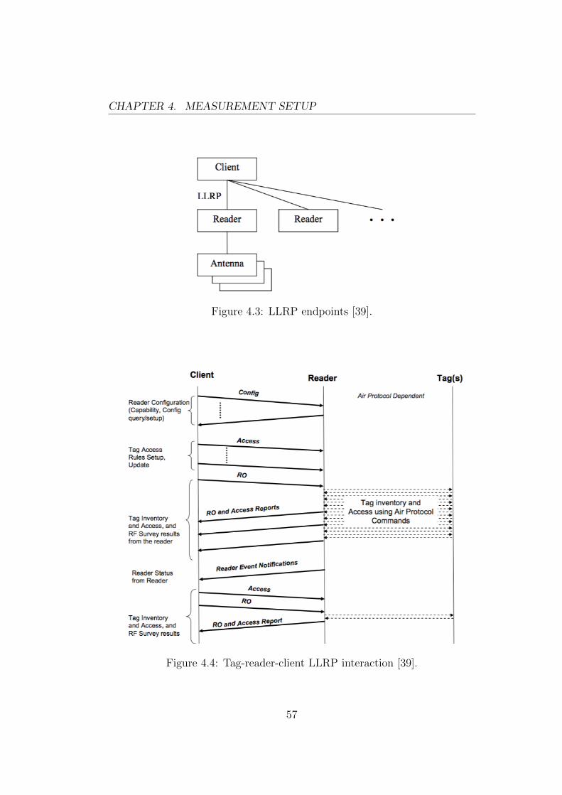
CHAPTER 4. MEASUREMENT SETUP
Figure 4.3: LLRP endpoints [39].
Figure 4.4: Tag-reader-client LLRP interaction [39].
57
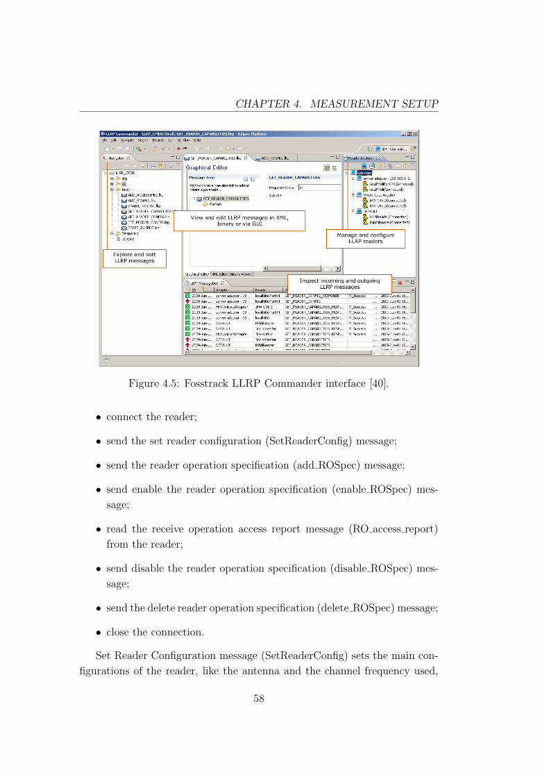
CHAPTER 4. MEASUREMENT SETUP
Figure 4.5: Fosstrack LLRP Commander interface [40].
• connect the reader;
• send the set reader configuration (SetReaderConfig) message;
• send the reader operation specification (add ROSpec) message;
• send enable the reader operation specification (enable ROSpec) mes-
sage;
• read the receive operation access report message (RO access report)
from the reader;
• send disable the reader operation specification (disable ROSpec) mes-
sage;
• send the delete reader operation specification (delete ROSpec) message;
• close the connection.
Set Reader Configuration message (SetReaderConfig) sets the main con-
figurations of the reader, like the antenna and the channel frequency used,
58
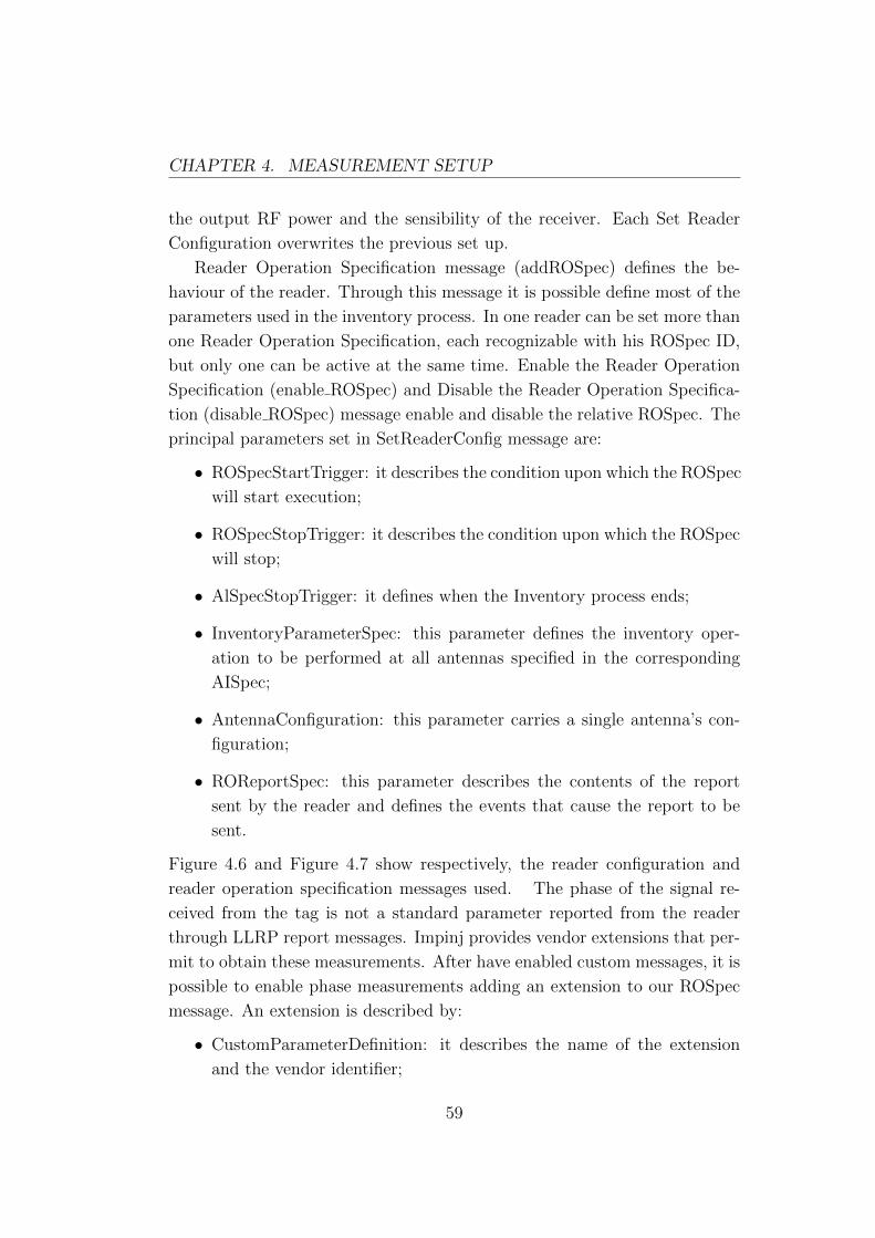
CHAPTER 4. MEASUREMENT SETUP
the output RF power and the sensibility of the receiver. Each Set Reader
Configuration overwrites the previous set up.
Reader Operation Specification message (addROSpec) defines the be-
haviour of the reader. Through this message it is possible define most of the
parameters used in the inventory process. In one reader can be set more than
one Reader Operation Specification, each recognizable with his ROSpec ID,
but only one can be active at the same time. Enable the Reader Operation
Specification (enable ROSpec) and Disable the Reader Operation Specifica-
tion (disable ROSpec) message enable and disable the relative ROSpec. The
principal parameters set in SetReaderConfig message are:
• ROSpecStartTrigger: it describes the condition upon which the ROSpec
will start execution;
• ROSpecStopTrigger: it describes the condition upon which the ROSpec
will stop;
• AlSpecStopTrigger: it defines when the Inventory process ends;
• InventoryParameterSpec: this parameter defines the inventory oper-
ation to be performed at all antennas specified in the corresponding
AISpec;
• AntennaConfiguration: this parameter carries a single antenna’s con-
figuration;
• ROReportSpec: this parameter describes the contents of the report
sent by the reader and defines the events that cause the report to be
sent.
Figure 4.6 and Figure 4.7 show respectively, the reader configuration and
reader operation specification messages used. The phase of the signal re-
ceived from the tag is not a standard parameter reported from the reader
through LLRP report messages. Impinj provides vendor extensions that per-
mit to obtain these measurements. After have enabled custom messages, it is
possible to enable phase measurements adding an extension to our ROSpec
message. An extension is described by:
• CustomParameterDefinition: it describes the name of the extension
and the vendor identifier;
59

CHAPTER 4. MEASUREMENT SETUP
Figure 4.6: Set Reader Configuration message used.
60
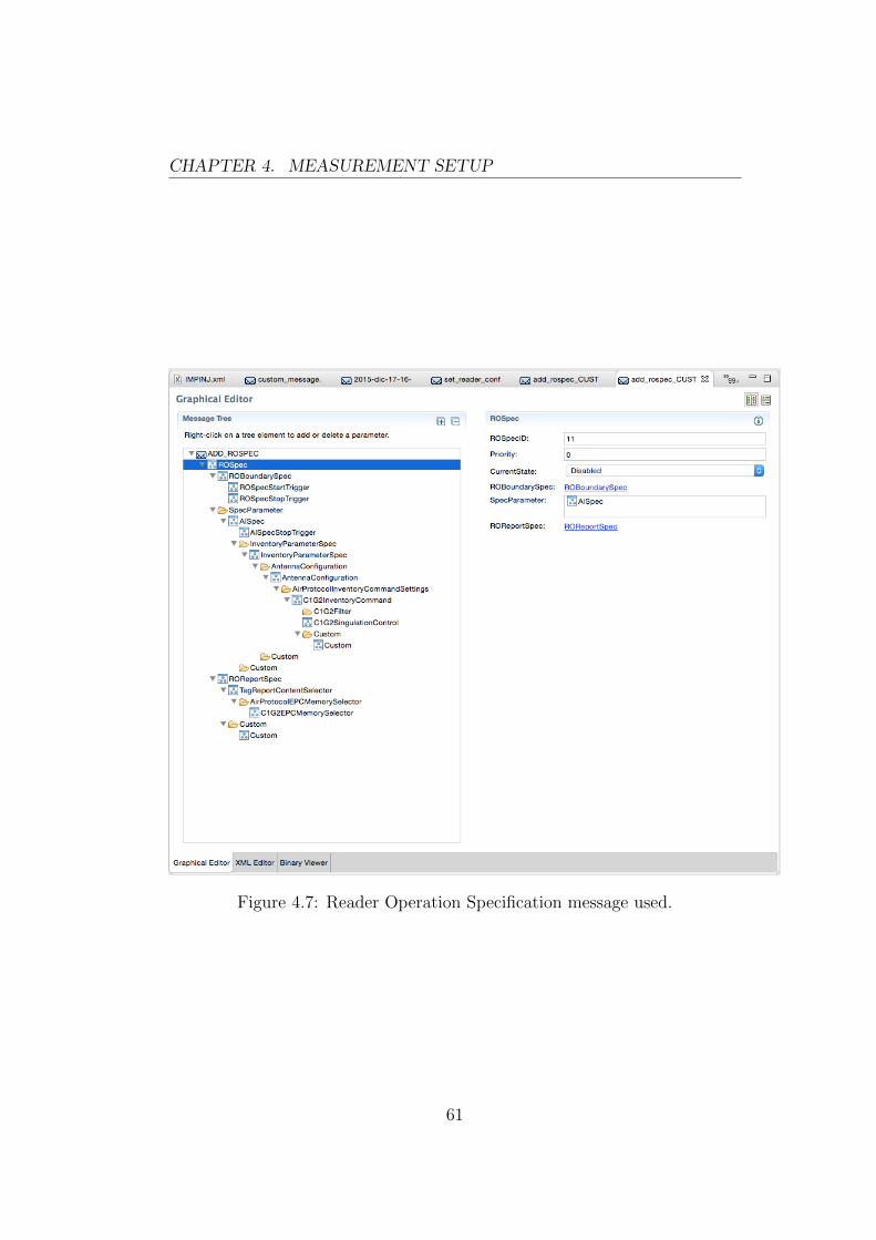
CHAPTER 4. MEASUREMENT SETUP
Figure 4.7: Reader Operation Specification message used.
61
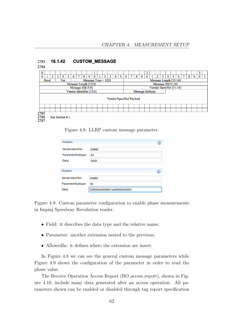
CHAPTER 4. MEASUREMENT SETUP
Figure 4.8: LLRP custom message parameter.
Figure 4.9: Custom parameter configuration to enable phase measurements
in Impinj Speedway Revolution reader.
• Field: it describes the data type and the relative name;
• Parameter: another extension nested to the previous;
• AllowedIn: it defines where the extension are insert.
In Figure 4.8 we can see the general custom message parameters while
Figure 4.9 shows the configuration of the parameter in order to read the
phase value.
The Receive Operation Access Report (RO access report), shown in Fig-
ure 4.10, include many data generated after an access operation. All pa-
rameters shown can be enabled or disabled through tag report specification
62
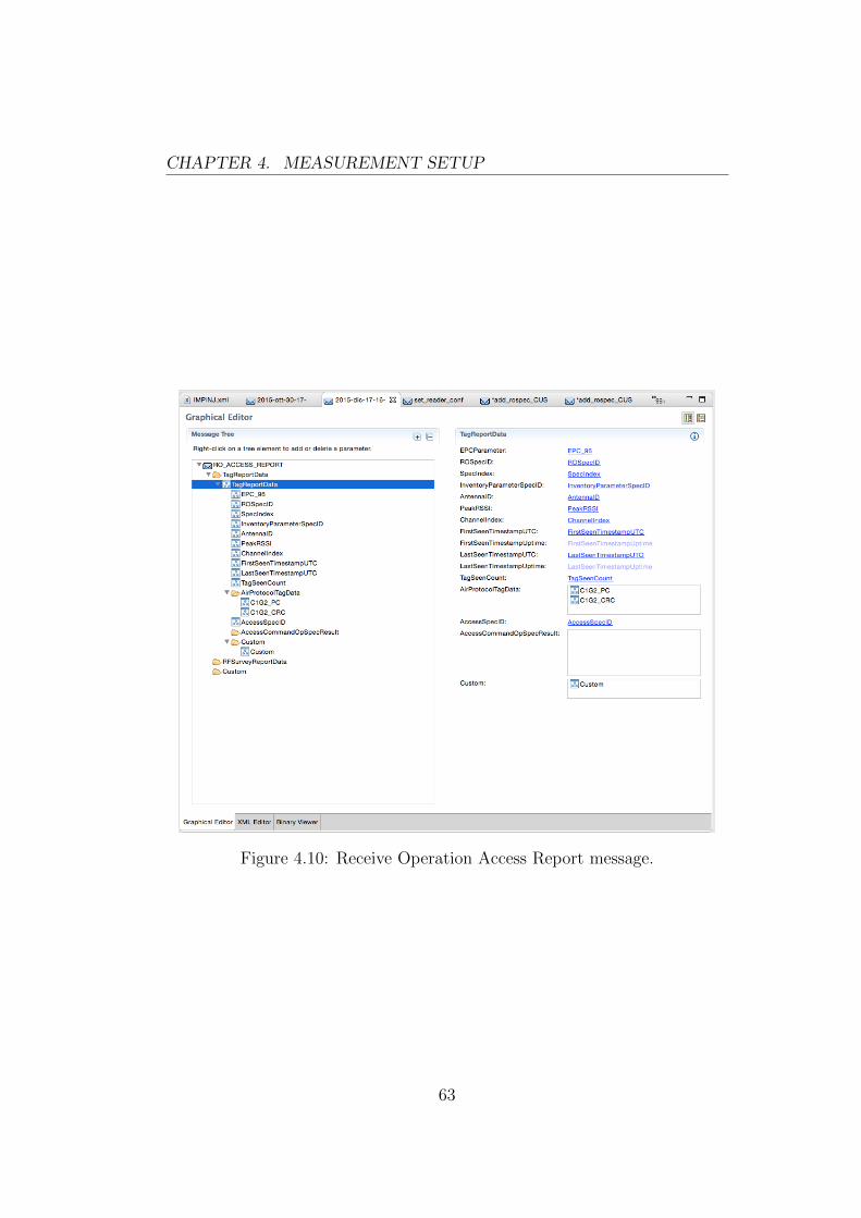
CHAPTER 4. MEASUREMENT SETUP
Figure 4.10: Receive Operation Access Report message.
63
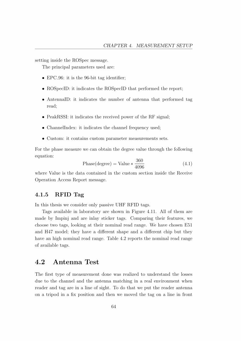
CHAPTER 4. MEASUREMENT SETUP
setting inside the ROSpec message.
The principal parameters used are:
• EPC 96: it is the 96-bit tag identifier;
• ROSpecID: it indicates the ROSpecID that performed the report;
• AntennaID: it indicates the number of antenna that performed tag
read;
• PeakRSSI: it indicates the received power of the RF signal;
• ChannelIndex: it indicates the channel frequency used;
• Custom: it contains custom parameter measurements sets.
For the phase measure we can obtain the degree value through the following
equation:
Phase(degree) = Value ∗ 360
4096(4.1)
where Value is the data contained in the custom section inside the Receive
Operation Access Report message.
4.1.5 RFID Tag
In this thesis we consider only passive UHF RFID tags.
Tags available in laboratory are shown in Figure 4.11. All of them are
made by Impinj and are inlay sticker tags. Comparing their features, we
choose two tags, looking at their nominal read range. We have chosen E51
and H47 model; they have a different shape and a different chip but they
have an high nominal read range. Table 4.2 reports the nominal read range
of available tags.
4.2 Antenna Test
The first type of measurement done was realized to understand the losses
due to the channel and the antenna matching in a real environment when
reader and tag are in a line of sight. To do that we put the reader antenna
on a tripod in a fix position and then we moved the tag on a line in front
64
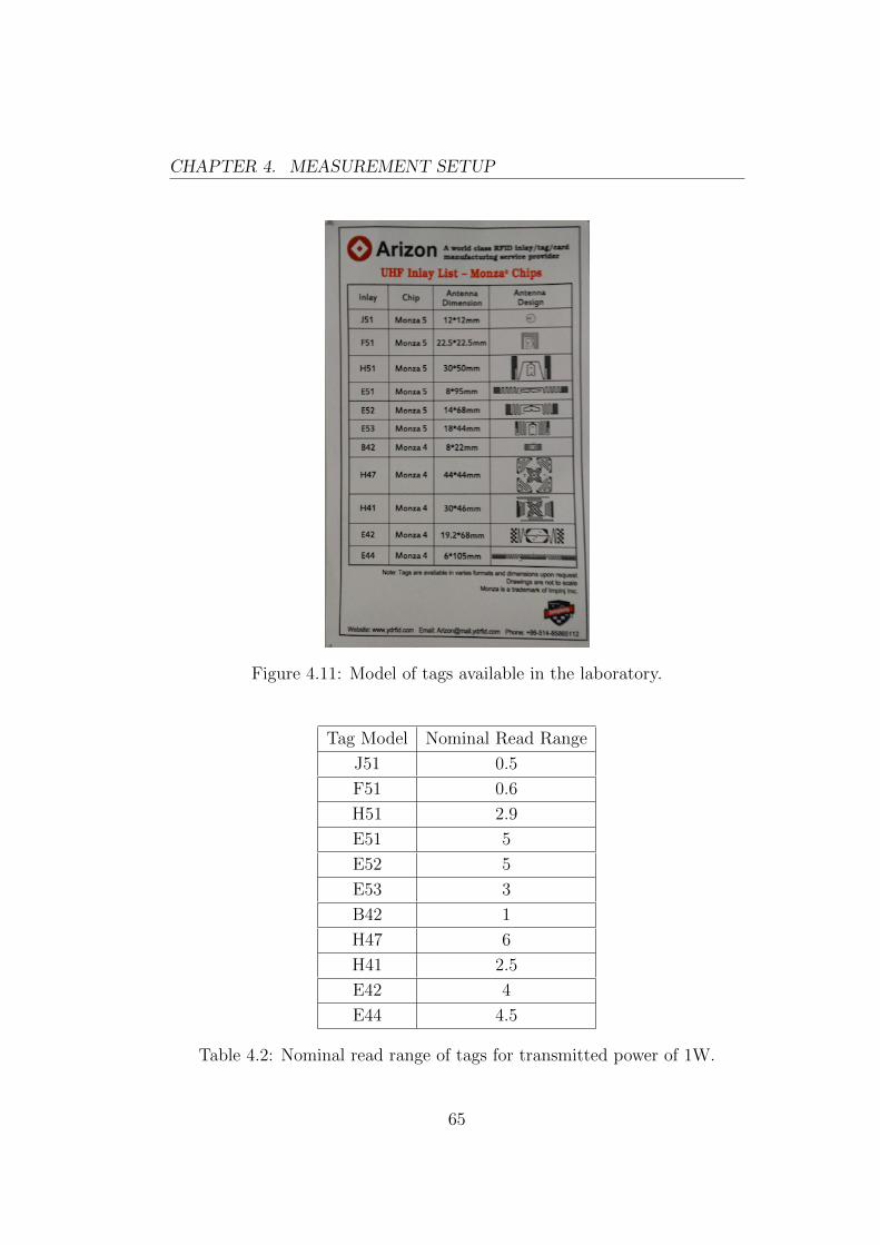
CHAPTER 4. MEASUREMENT SETUP
Figure 4.11: Model of tags available in the laboratory.
Tag Model Nominal Read Range
J51 0.5
F51 0.6
H51 2.9
E51 5
E52 5
E53 3
B42 1
H47 6
H41 2.5
E42 4
E44 4.5
Table 4.2: Nominal read range of tags for transmitted power of 1W.
65
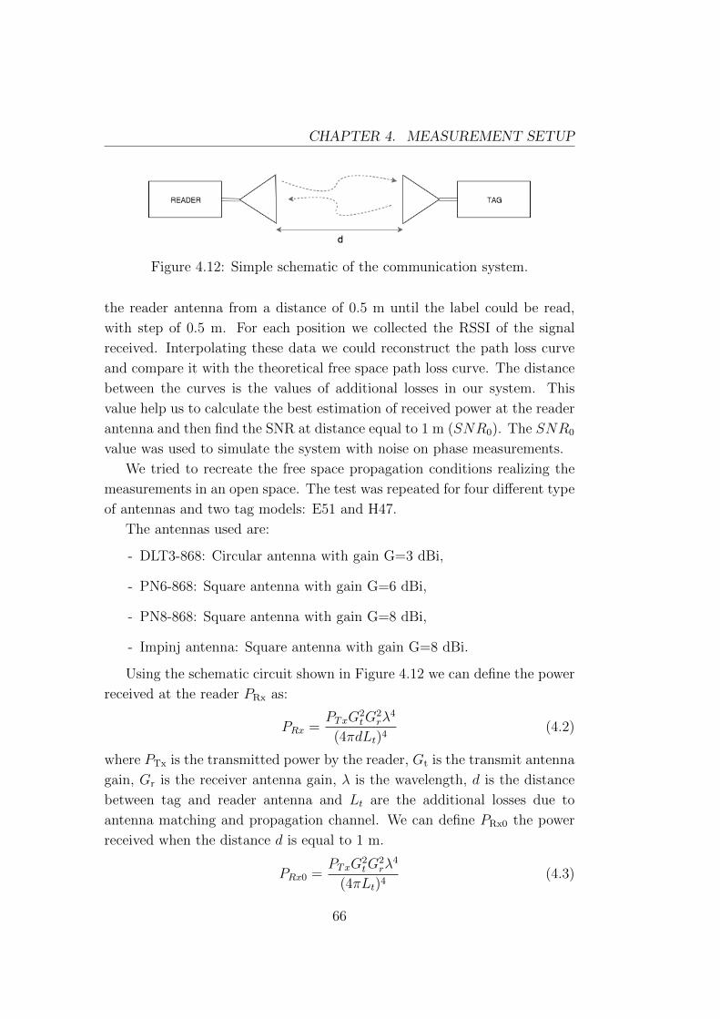
CHAPTER 4. MEASUREMENT SETUP
Figure 4.12: Simple schematic of the communication system.
the reader antenna from a distance of 0.5 m until the label could be read,
with step of 0.5 m. For each position we collected the RSSI of the signal
received. Interpolating these data we could reconstruct the path loss curve
and compare it with the theoretical free space path loss curve. The distance
between the curves is the values of additional losses in our system. This
value help us to calculate the best estimation of received power at the reader
antenna and then find the SNR at distance equal to 1 m (SNR0). The SNR0
value was used to simulate the system with noise on phase measurements.
We tried to recreate the free space propagation conditions realizing the
measurements in an open space. The test was repeated for four different type
of antennas and two tag models: E51 and H47.
The antennas used are:
- DLT3-868: Circular antenna with gain G=3 dBi,
- PN6-868: Square antenna with gain G=6 dBi,
- PN8-868: Square antenna with gain G=8 dBi,
- Impinj antenna: Square antenna with gain G=8 dBi.
Using the schematic circuit shown in Figure 4.12 we can define the power
received at the reader PRx as:
PRx =PTxG
2tG
2rλ
4
(4πdLt)4(4.2)
where PTx is the transmitted power by the reader, Gt is the transmit antenna
gain, Gr is the receiver antenna gain, λ is the wavelength, d is the distance
between tag and reader antenna and Lt are the additional losses due to
antenna matching and propagation channel. We can define PRx0 the power
received when the distance d is equal to 1 m.
PRx0 =PTxG
2tG
2rλ
4
(4πLt)4(4.3)
66
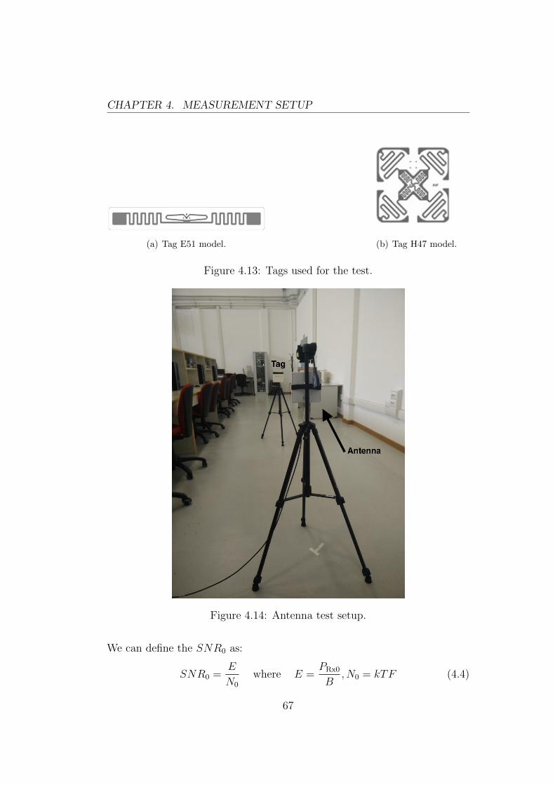
CHAPTER 4. MEASUREMENT SETUP
(a) Tag E51 model. (b) Tag H47 model.
Figure 4.13: Tags used for the test.
Figure 4.14: Antenna test setup.
We can define the SNR0 as:
SNR0 =E
N0
where E =PRx0
B,N0 = kTF (4.4)
67
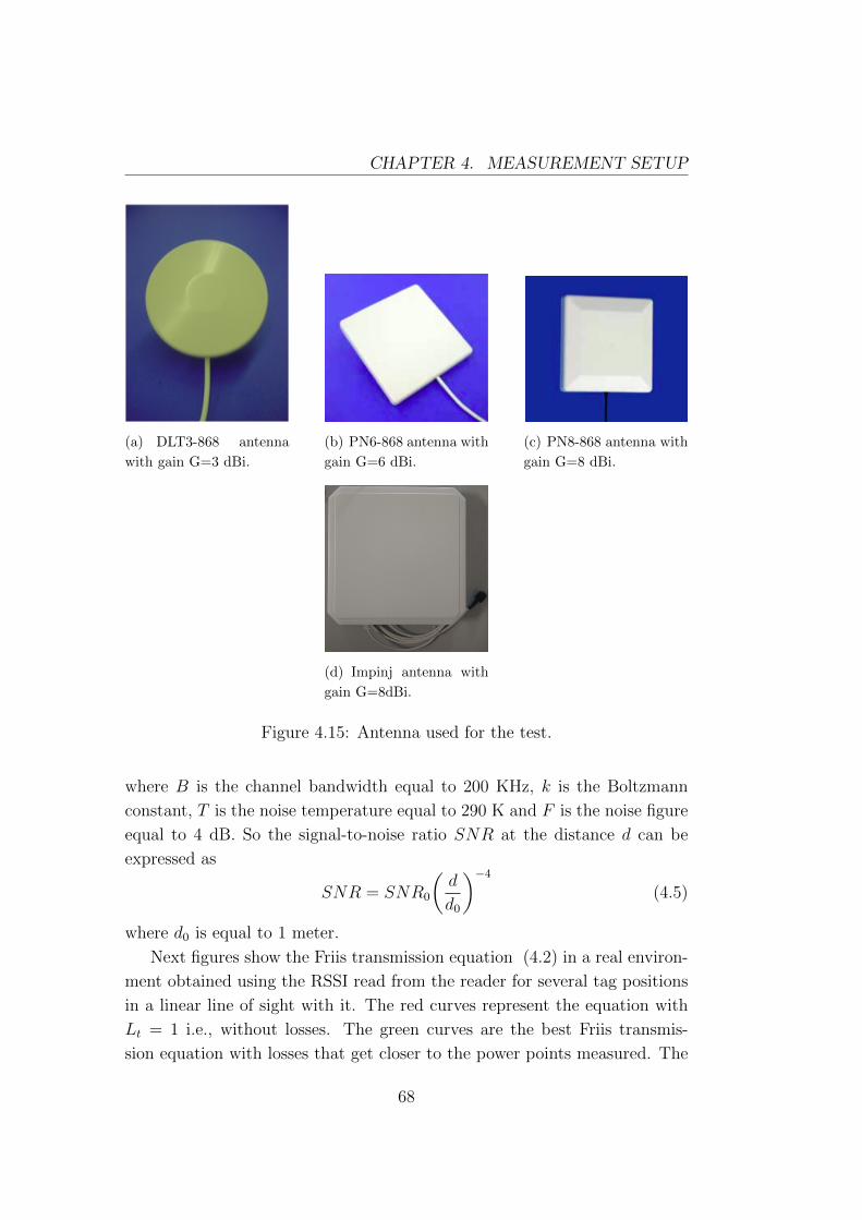
CHAPTER 4. MEASUREMENT SETUP
(a) DLT3-868 antenna
with gain G=3 dBi.
(b) PN6-868 antenna with
gain G=6 dBi.
(c) PN8-868 antenna with
gain G=8 dBi.
(d) Impinj antenna with
gain G=8dBi.
Figure 4.15: Antenna used for the test.
where B is the channel bandwidth equal to 200 KHz, k is the Boltzmann
constant, T is the noise temperature equal to 290 K and F is the noise figure
equal to 4 dB. So the signal-to-noise ratio SNR at the distance d can be
expressed as
SNR = SNR0
(d
d0
)−4
(4.5)
where d0 is equal to 1 meter.
Next figures show the Friis transmission equation (4.2) in a real environ-
ment obtained using the RSSI read from the reader for several tag positions
in a linear line of sight with it. The red curves represent the equation with
Lt = 1 i.e., without losses. The green curves are the best Friis transmis-
sion equation with losses that get closer to the power points measured. The
68
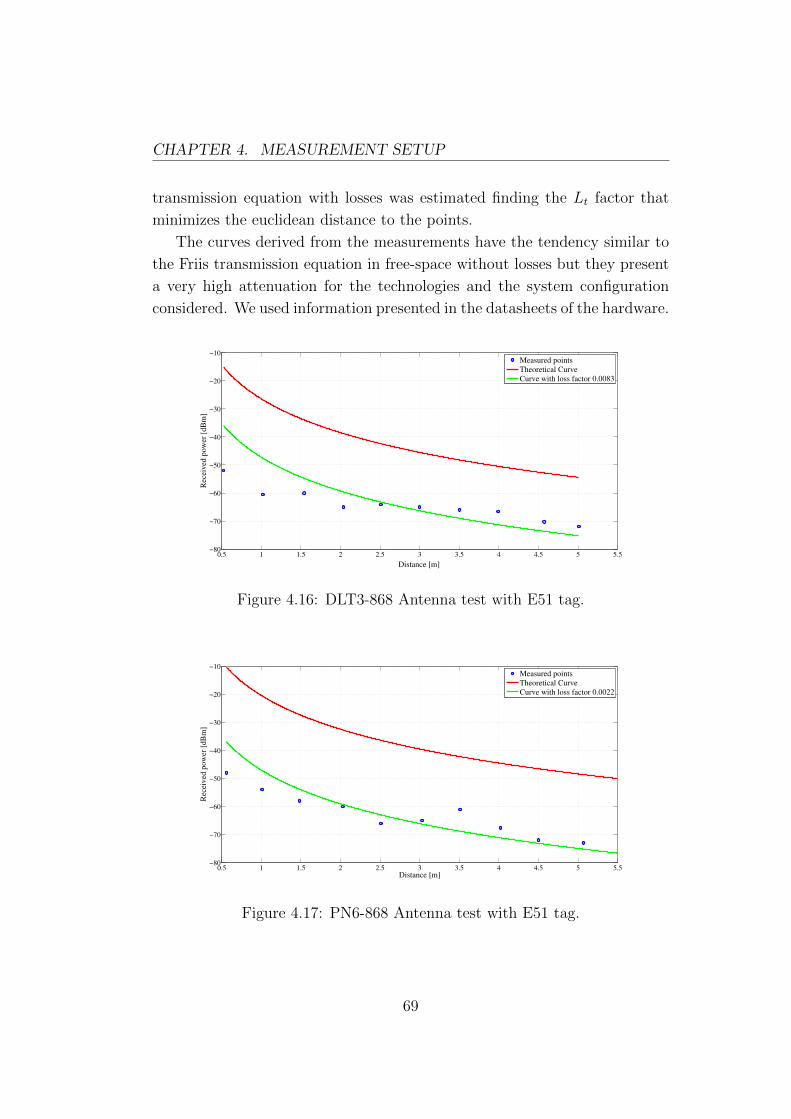
CHAPTER 4. MEASUREMENT SETUP
transmission equation with losses was estimated finding the Lt factor that
minimizes the euclidean distance to the points.
The curves derived from the measurements have the tendency similar to
the Friis transmission equation in free-space without losses but they present
a very high attenuation for the technologies and the system configuration
considered. We used information presented in the datasheets of the hardware.
0.5 1 1.5 2 2.5 3 3.5 4 4.5 5 5.5−80
−70
−60
−50
−40
−30
−20
−10
Distance [m]
Rec
eived
pow
er [
dB
m]
Measured points
Theoretical Curve
Curve with loss factor 0.0083
Figure 4.16: DLT3-868 Antenna test with E51 tag.
0.5 1 1.5 2 2.5 3 3.5 4 4.5 5 5.5−80
−70
−60
−50
−40
−30
−20
−10
Distance [m]
Rec
eived
pow
er [
dB
m]
Measured points
Theoretical Curve
Curve with loss factor 0.0022
Figure 4.17: PN6-868 Antenna test with E51 tag.
69
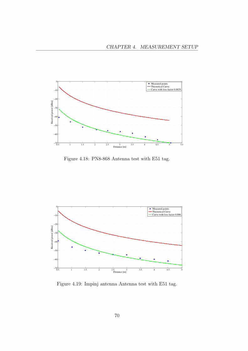
CHAPTER 4. MEASUREMENT SETUP
0.5 1 1.5 2 2.5 3 3.5 4 4.5 5 5.5−70
−60
−50
−40
−30
−20
−10
0
Distance [m]
Rec
eived
pow
er [
dB
m]
Measured points
Theoretical Curve
Curve with loss factor 0.0029
Figure 4.18: PN8-868 Antenna test with E51 tag.
0.5 1 1.5 2 2.5 3 3.5 4 4.5 5−70
−60
−50
−40
−30
−20
−10
0
Distance [m]
Rec
eived
pow
er [
dB
m]
Measured points
Theoretical Curve
Curve with loss factor 0.006
Figure 4.19: Impinj antenna Antenna test with E51 tag.
70
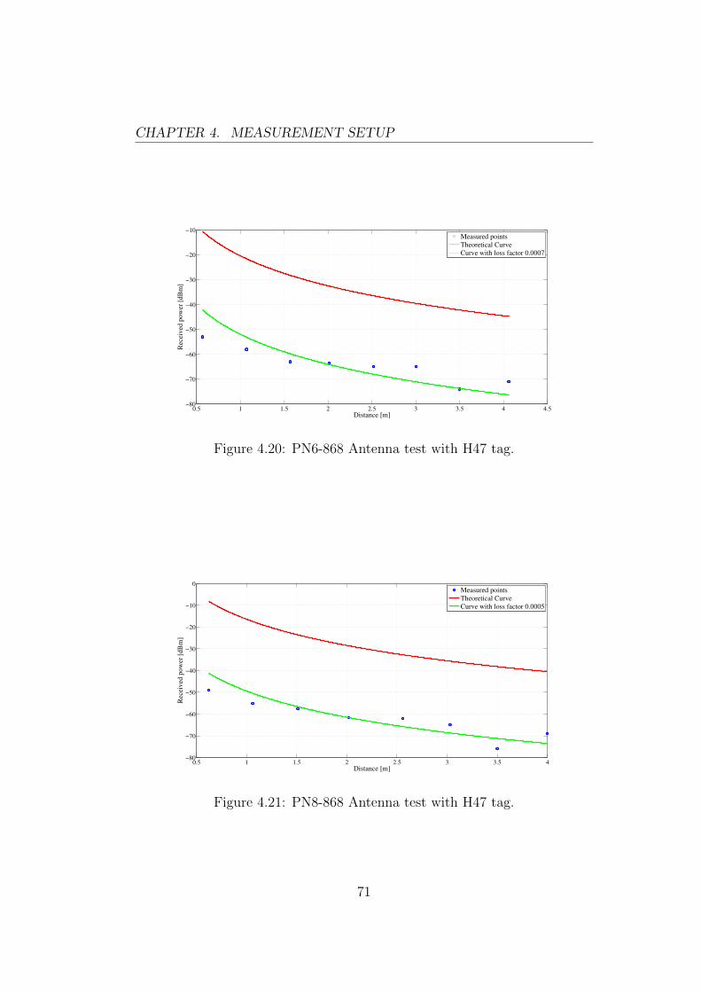
CHAPTER 4. MEASUREMENT SETUP
0.5 1 1.5 2 2.5 3 3.5 4 4.5−80
−70
−60
−50
−40
−30
−20
−10
Distance [m]
Rec
eived
pow
er [
dB
m]
Measured points
Theoretical Curve
Curve with loss factor 0.0007
Figure 4.20: PN6-868 Antenna test with H47 tag.
0.5 1 1.5 2 2.5 3 3.5 4−80
−70
−60
−50
−40
−30
−20
−10
0
Distance [m]
Rec
eived
pow
er [
dB
m]
Measured points
Theoretical Curve
Curve with loss factor 0.0005
Figure 4.21: PN8-868 Antenna test with H47 tag.
71
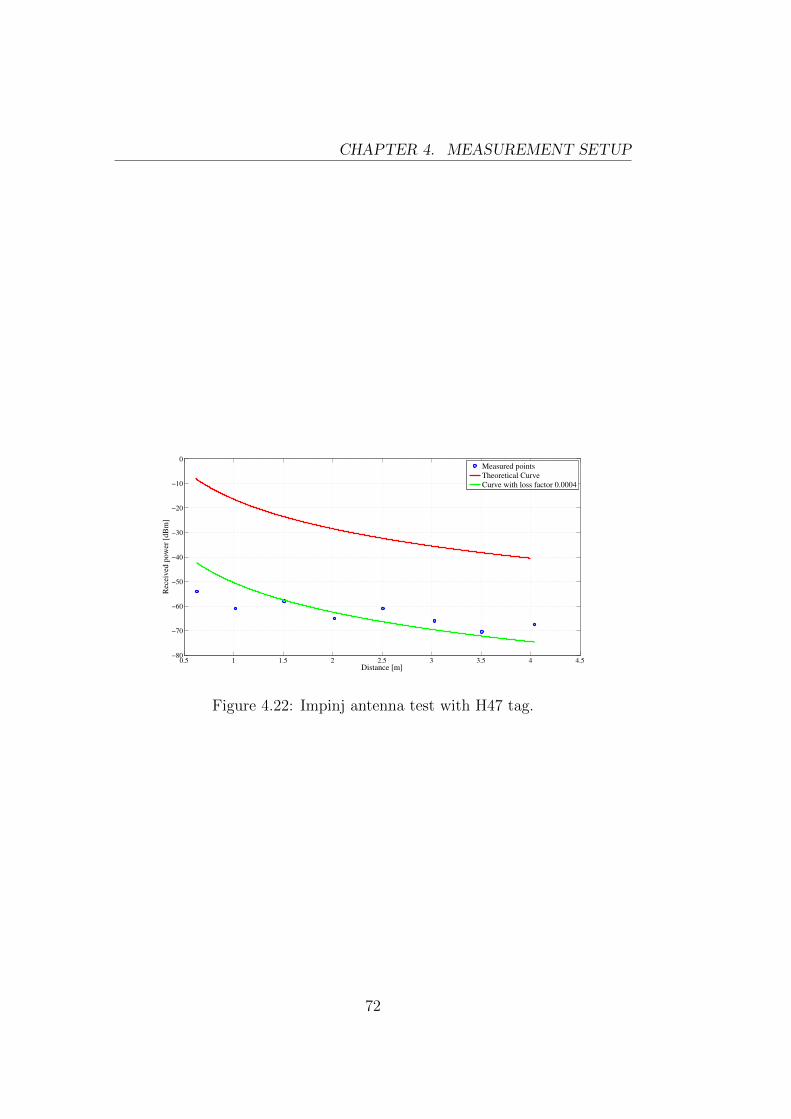
CHAPTER 4. MEASUREMENT SETUP
0.5 1 1.5 2 2.5 3 3.5 4 4.5−80
−70
−60
−50
−40
−30
−20
−10
0
Distance [m]
Rec
eived
pow
er [
dB
m]
Measured points
Theoretical Curve
Curve with loss factor 0.0004
Figure 4.22: Impinj antenna test with H47 tag.
72
Chapter 5
Measurement Results
5.1 Linear trajectory
After the simulative approach we decided to test the algorithm in a real
environment. The first test concerned the lateral relative movements of the
reader with respect to the tag. Our questions were: how long the tag can be
read while the reader is moving laterally with respect to it? Using the phase
measurements, can the tag be located correctly? Which algorithm does have
the best performance?
For an easier procedure of measurement we placed the reader antenna
fixed in the position of 4.65 m and moved the tag back and forth in a linear
trajectory in front of the reader. This situation is equal of the corresponding
used in simulations, where the tag was fixed and the reader in movement,
because what it is important is the relative motion among them. Tag was
moved with step of 0.1 m. For each position the phase and the RSS values
was taken as the mean of ten different measures. The test was repeated
for three different tag-reader frontal distances, 1 m, 2 m, 3 m and for two
antennas: PN6-868 model with 6 dBi gain and PN8-868 model with 8 dBi
gain.
The procedure can be summarized as:
1. Put the reader antenna in the fix point with coordinate 4.65 m;
2. Put the tag in front of the reader antenna at the desired distance;
73
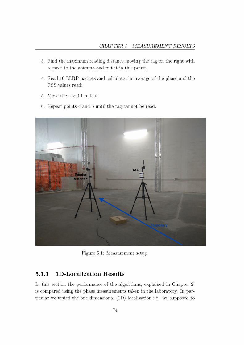
CHAPTER 5. MEASUREMENT RESULTS
3. Find the maximum reading distance moving the tag on the right with
respect to the antenna and put it in this point;
4. Read 10 LLRP packets and calculate the average of the phase and the
RSS values read;
5. Move the tag 0.1 m left.
6. Repeat points 4 and 5 until the tag cannot be read.
Figure 5.1: Measurement setup.
5.1.1 1D-Localization Results
In this section the performance of the algorithms, explained in Chapter 2.
is compared using the phase measurements taken in the laboratory. In par-
ticular we tested the one dimensional (1D) localization i.e., we supposed to
74
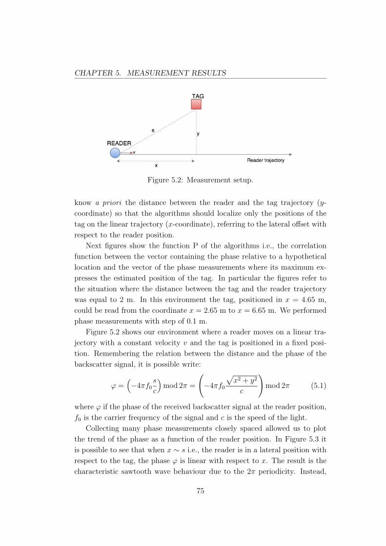
CHAPTER 5. MEASUREMENT RESULTS
Figure 5.2: Measurement setup.
know a priori the distance between the reader and the tag trajectory (y-
coordinate) so that the algorithms should localize only the positions of the
tag on the linear trajectory (x-coordinate), referring to the lateral offset with
respect to the reader position.
Next figures show the function P of the algorithms i.e., the correlation
function between the vector containing the phase relative to a hypothetical
location and the vector of the phase measurements where its maximum ex-
presses the estimated position of the tag. In particular the figures refer to
the situation where the distance between the tag and the reader trajectory
was equal to 2 m. In this environment the tag, positioned in x = 4.65 m,
could be read from the coordinate x = 2.65 m to x = 6.65 m. We performed
phase measurements with step of 0.1 m.
Figure 5.2 shows our environment where a reader moves on a linear tra-
jectory with a constant velocity v and the tag is positioned in a fixed posi-
tion. Remembering the relation between the distance and the phase of the
backscatter signal, it is possible write:
ϕ =(−4πf0
s
c
)mod 2π =
(−4πf0
√x2 + y2
c
)mod 2π (5.1)
where ϕ if the phase of the received backscatter signal at the reader position,
f0 is the carrier frequency of the signal and c is the speed of the light.
Collecting many phase measurements closely spaced allowed us to plot
the trend of the phase as a function of the reader position. In Figure 5.3 it
is possible to see that when x ∼ s i.e., the reader is in a lateral position with
respect to the tag, the phase ϕ is linear with respect to x. The result is the
characteristic sawtooth wave behaviour due to the 2π periodicity. Instead,
75
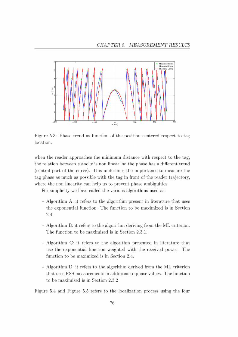
CHAPTER 5. MEASUREMENT RESULTS
−300 −200 −100 0 100 200 3000
1
2
3
4
5
6
7
x [cm]
ϕ[rad]
Measured Points
Measured Curve
Theorical Curve
Figure 5.3: Phase trend as function of the position centered respect to tag
location.
when the reader approaches the minimum distance with respect to the tag,
the relation between s and x is non linear, so the phase has a different trend
(central part of the curve). This underlines the importance to measure the
tag phase as much as possible with the tag in front of the reader trajectory,
where the non linearity can help us to prevent phase ambiguities.
For simplicity we have called the various algorithms used as:
- Algorithm A: it refers to the algorithm present in literature that uses
the exponential function. The function to be maximized is in Section
2.4.
- Algorithm B: it refers to the algorithm deriving from the ML criterion.
The function to be maximized is in Section 2.3.1.
- Algorithm C: it refers to the algorithm presented in literature that
use the exponential function weighted with the received power. The
function to be maximized is in Section 2.4.
- Algorithm D: it refers to the algorithm derived from the ML criterion
that uses RSS measurements in additions to phase values. The function
to be maximized is in Section 2.3.2
Figure 5.4 and Figure 5.5 refers to the localization process using the four
76
CHAPTER 5. MEASUREMENT RESULTS
algorithms propose. Specifically, they show the functions whose maximum
indicates the tag position.
From Figure 5.6 to Figure 5.15 the localization is performed considering
the different algorithms using a portion of the total trajectory. We have
chosen only few central phase measurements (5, 7, 9 or 11 values) in order
to use values that belong to the non linear zone of the characteristic phase
trend; so the phase ambiguities could be limited. In general, decreasing the
number of phase measures N and consequently the length L of the trajectory
produces smoother correlation functions where the maximum location is more
ambiguous. This effect is amplified in the algorithms presented in literature,
that use the exponential function. Usually the algorithm B presents a sharper
principal peak than the other methods.
Figure 5.16 and Figure 5.18 show the localization of the tag using phase
measurements spaced respectively 0.2 meters and 0.3 meters along overall
trajectory.
In general, in all configurations, the algorithm D leads to a wrong local-
ization. The resultant correlation function is almost flat and presents a peak
not in the tag position. This behavior could be explained with the low reli-
ability and the randomness of the RSS values. In the 1D localization when
the distance between the reader trajectory and the tag is equal to 3 meters,
the function is still flat but it leads to a correct localization (see Appendix
A).
RSS values work better in the algorithm C where the function to be
maximized is exponential.
Table 5.1 and Table 5.2 present the results and the RMSE of the localiza-
tion for different configurations. N indicates the number of phase measures
used and L is the equivalent length of the trajectory. Looking at the table,
it is possible to see that the algorithm B, using the ML criterion, has for all
the configurations a performance equal or better than that of the algorithm
A. Only in the configuration with N = 5 and L = 0.8 m it presents a wrong
localization due to a secondary peak that grews decreasing the number of
phase values.
Another test done concerned the choice of the best phase values. In order
to use only the more reliable measurements, we implemented a threshold
model where a phase value was used in the algorithm only if its received
77
CHAPTER 5. MEASUREMENT RESULTS
power level satisfied a determined threshold. Table 5.3 and Table 5.4 show
the results of this analysis. A received phase value is used in the localization
process only if the corresponding RSS is included between the maximum
RSS along the trajectory and the latter less the threshold. The threshold
was not set in a unique manner, but relative to the maximum signal power
along the trajectory. Decreasing the threshold level less phase values are
used in the algorithms. Looking at the tables we notice that the localization
results with a threshold equal to 10-12 dB generally is equal or better than
the localization with all phase values measured. A threshold equal to 2 dB
causes a high RMSE because few phase measurements are collected.
The last experiment done in the 1D localization localization scenario con-
siders, a Monte Carlo simulations. Using one of the configurations seen be-
fore, in particular N = 7 and L = 0.6 m, Gaussian noise was added to the
reader position in order to discover the performance of the algorithms when
the information about the position is not precise. The test was repeated for
several noise variances. The results, shown in Table 5.5 and Table 5.6, reveal
that the noise on the reader position does not degrade significantly the local-
ization estimation provided that its standard deviation is lower than 0.032
m. Increasing the noise variance the resulting RMSE raises considerably.
78
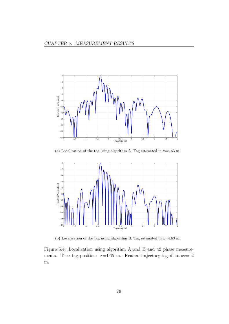
CHAPTER 5. MEASUREMENT RESULTS
3 3.5 4 4.5 5 5.5 6 6.5 7 7.5 8−20
−18
−16
−14
−12
−10
−8
−6
−4
−2
0
Trajectory [m]
Funct
ion P
norm
aliz
ed
(a) Localization of the tag using algorithm A. Tag estimated in x=4.63 m.
3 3.5 4 4.5 5 5.5 6 6.5 7 7.5 8−20
−18
−16
−14
−12
−10
−8
−6
−4
−2
0
Trajectory [m]
Funct
ion P
norm
aliz
ed
(b) Localization of the tag using algorithm B. Tag estimated in x=4.63 m.
Figure 5.4: Localization using algorithm A and B and 42 phase measure-
ments. True tag position: x=4.65 m. Reader trajectory-tag distance= 2
m.
79
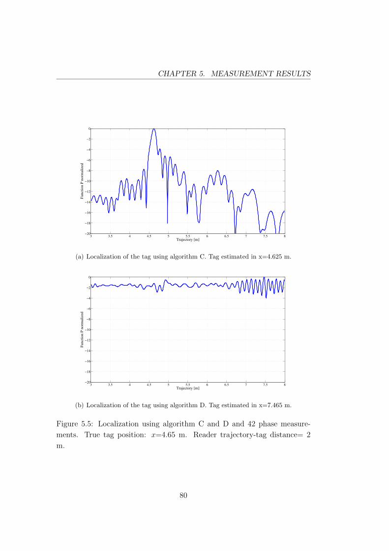
CHAPTER 5. MEASUREMENT RESULTS
3 3.5 4 4.5 5 5.5 6 6.5 7 7.5 8−20
−18
−16
−14
−12
−10
−8
−6
−4
−2
0
Trajectory [m]
Funct
ion P
norm
aliz
ed
(a) Localization of the tag using algorithm C. Tag estimated in x=4.625 m.
3 3.5 4 4.5 5 5.5 6 6.5 7 7.5 8−20
−18
−16
−14
−12
−10
−8
−6
−4
−2
0
Trajectory [m]
Funct
ion P
norm
aliz
ed
(b) Localization of the tag using algorithm D. Tag estimated in x=7.465 m.
Figure 5.5: Localization using algorithm C and D and 42 phase measure-
ments. True tag position: x=4.65 m. Reader trajectory-tag distance= 2
m.
80
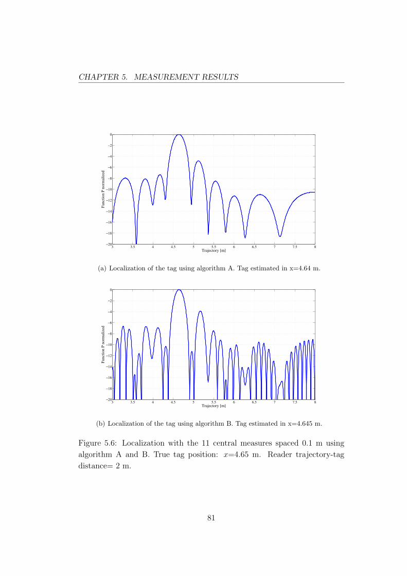
CHAPTER 5. MEASUREMENT RESULTS
3 3.5 4 4.5 5 5.5 6 6.5 7 7.5 8−20
−18
−16
−14
−12
−10
−8
−6
−4
−2
0
Trajectory [m]
Funct
ion P
norm
aliz
ed
(a) Localization of the tag using algorithm A. Tag estimated in x=4.64 m.
3 3.5 4 4.5 5 5.5 6 6.5 7 7.5 8−20
−18
−16
−14
−12
−10
−8
−6
−4
−2
0
Trajectory [m]
Funct
ion P
norm
aliz
ed
(b) Localization of the tag using algorithm B. Tag estimated in x=4.645 m.
Figure 5.6: Localization with the 11 central measures spaced 0.1 m using
algorithm A and B. True tag position: x=4.65 m. Reader trajectory-tag
distance= 2 m.
81
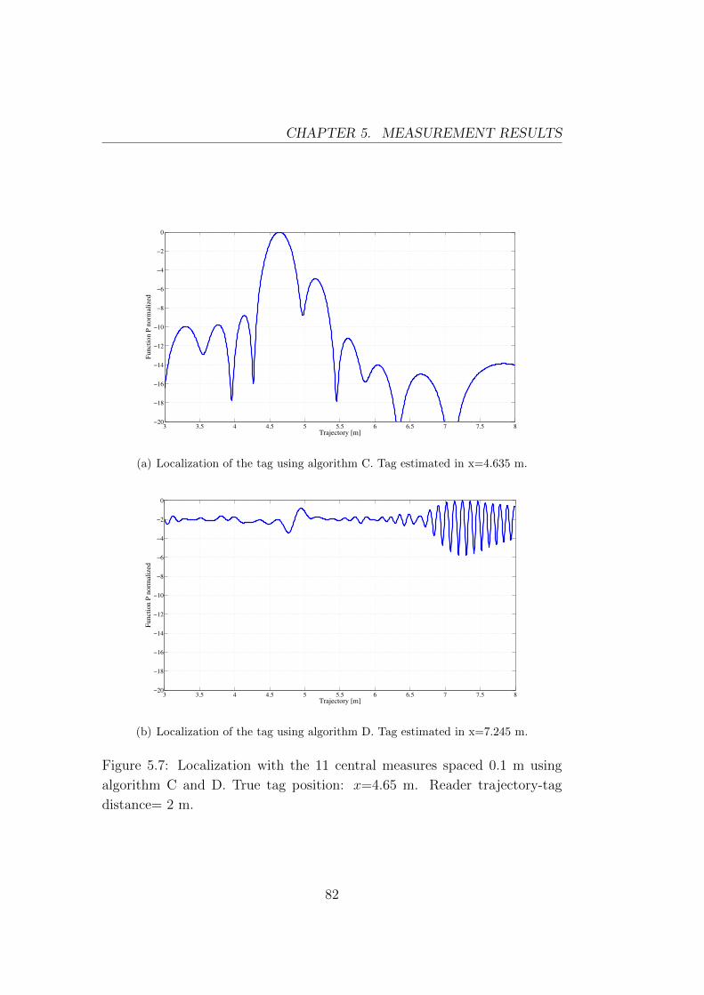
CHAPTER 5. MEASUREMENT RESULTS
3 3.5 4 4.5 5 5.5 6 6.5 7 7.5 8−20
−18
−16
−14
−12
−10
−8
−6
−4
−2
0
Trajectory [m]
Funct
ion P
norm
aliz
ed
(a) Localization of the tag using algorithm C. Tag estimated in x=4.635 m.
3 3.5 4 4.5 5 5.5 6 6.5 7 7.5 8−20
−18
−16
−14
−12
−10
−8
−6
−4
−2
0
Trajectory [m]
Funct
ion P
norm
aliz
ed
(b) Localization of the tag using algorithm D. Tag estimated in x=7.245 m.
Figure 5.7: Localization with the 11 central measures spaced 0.1 m using
algorithm C and D. True tag position: x=4.65 m. Reader trajectory-tag
distance= 2 m.
82
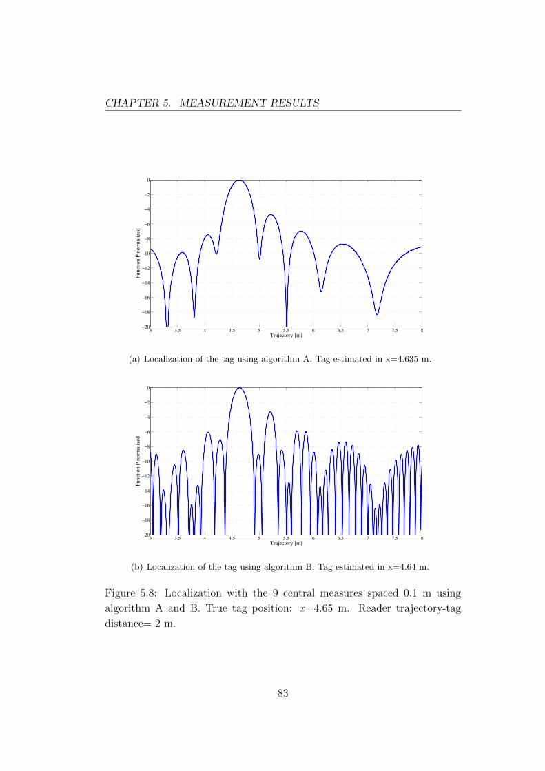
CHAPTER 5. MEASUREMENT RESULTS
3 3.5 4 4.5 5 5.5 6 6.5 7 7.5 8−20
−18
−16
−14
−12
−10
−8
−6
−4
−2
0
Trajectory [m]
Funct
ion P
norm
aliz
ed
(a) Localization of the tag using algorithm A. Tag estimated in x=4.635 m.
3 3.5 4 4.5 5 5.5 6 6.5 7 7.5 8−20
−18
−16
−14
−12
−10
−8
−6
−4
−2
0
Trajectory [m]
Funct
ion P
norm
aliz
ed
(b) Localization of the tag using algorithm B. Tag estimated in x=4.64 m.
Figure 5.8: Localization with the 9 central measures spaced 0.1 m using
algorithm A and B. True tag position: x=4.65 m. Reader trajectory-tag
distance= 2 m.
83
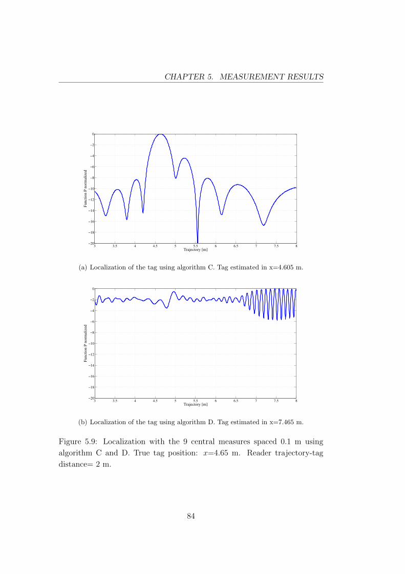
CHAPTER 5. MEASUREMENT RESULTS
3 3.5 4 4.5 5 5.5 6 6.5 7 7.5 8−20
−18
−16
−14
−12
−10
−8
−6
−4
−2
0
Trajectory [m]
Funct
ion P
norm
aliz
ed
(a) Localization of the tag using algorithm C. Tag estimated in x=4.605 m.
3 3.5 4 4.5 5 5.5 6 6.5 7 7.5 8−20
−18
−16
−14
−12
−10
−8
−6
−4
−2
0
Trajectory [m]
Funct
ion P
norm
aliz
ed
(b) Localization of the tag using algorithm D. Tag estimated in x=7.465 m.
Figure 5.9: Localization with the 9 central measures spaced 0.1 m using
algorithm C and D. True tag position: x=4.65 m. Reader trajectory-tag
distance= 2 m.
84
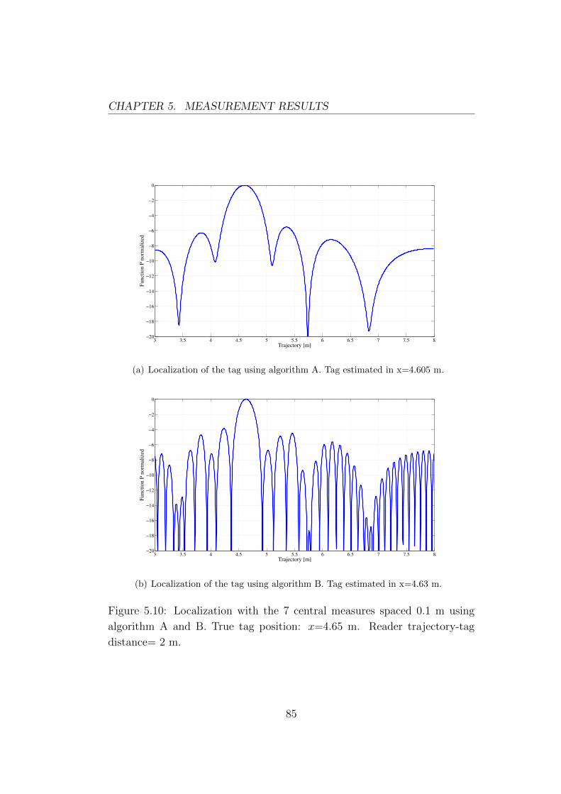
CHAPTER 5. MEASUREMENT RESULTS
3 3.5 4 4.5 5 5.5 6 6.5 7 7.5 8−20
−18
−16
−14
−12
−10
−8
−6
−4
−2
0
Trajectory [m]
Funct
ion P
norm
aliz
ed
(a) Localization of the tag using algorithm A. Tag estimated in x=4.605 m.
3 3.5 4 4.5 5 5.5 6 6.5 7 7.5 8−20
−18
−16
−14
−12
−10
−8
−6
−4
−2
0
Trajectory [m]
Funct
ion P
norm
aliz
ed
(b) Localization of the tag using algorithm B. Tag estimated in x=4.63 m.
Figure 5.10: Localization with the 7 central measures spaced 0.1 m using
algorithm A and B. True tag position: x=4.65 m. Reader trajectory-tag
distance= 2 m.
85
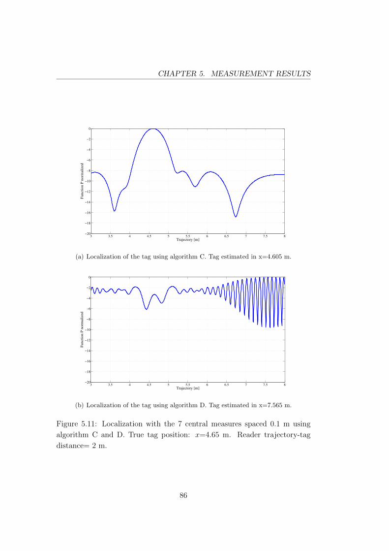
CHAPTER 5. MEASUREMENT RESULTS
3 3.5 4 4.5 5 5.5 6 6.5 7 7.5 8−20
−18
−16
−14
−12
−10
−8
−6
−4
−2
0
Trajectory [m]
Funct
ion P
norm
aliz
ed
(a) Localization of the tag using algorithm C. Tag estimated in x=4.605 m.
3 3.5 4 4.5 5 5.5 6 6.5 7 7.5 8−20
−18
−16
−14
−12
−10
−8
−6
−4
−2
0
Trajectory [m]
Funct
ion P
norm
aliz
ed
(b) Localization of the tag using algorithm D. Tag estimated in x=7.565 m.
Figure 5.11: Localization with the 7 central measures spaced 0.1 m using
algorithm C and D. True tag position: x=4.65 m. Reader trajectory-tag
distance= 2 m.
86
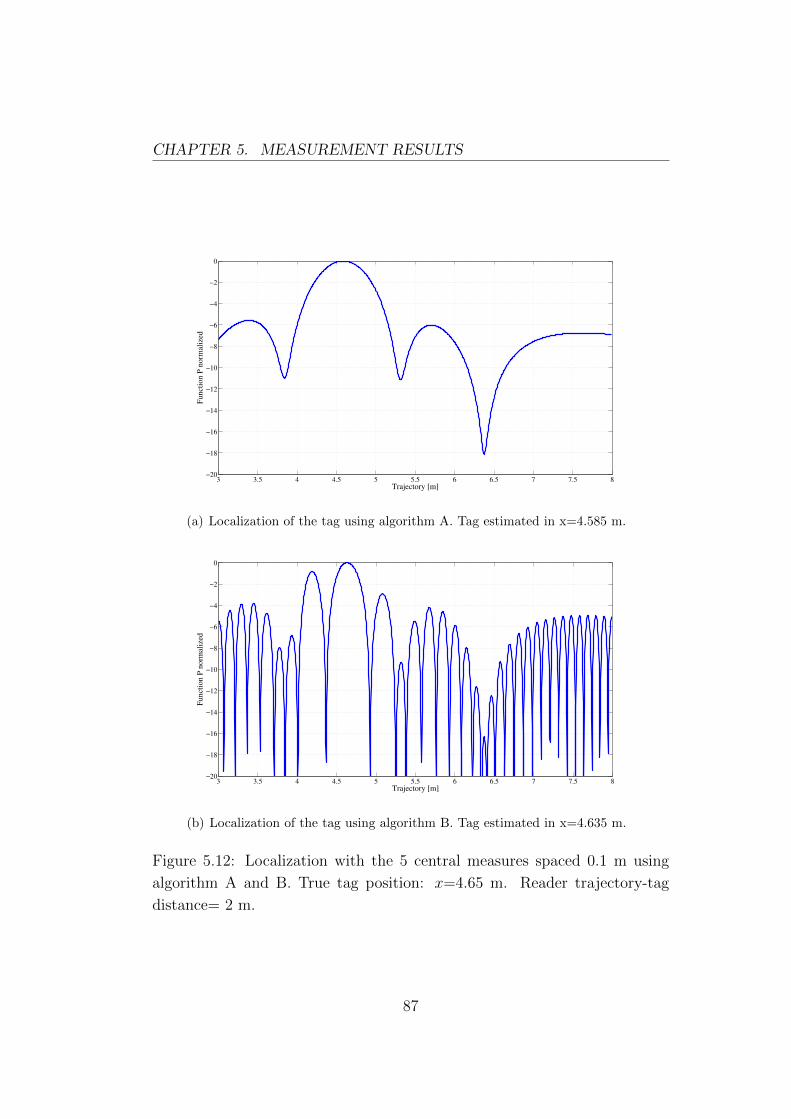
CHAPTER 5. MEASUREMENT RESULTS
3 3.5 4 4.5 5 5.5 6 6.5 7 7.5 8−20
−18
−16
−14
−12
−10
−8
−6
−4
−2
0
Trajectory [m]
Funct
ion P
norm
aliz
ed
(a) Localization of the tag using algorithm A. Tag estimated in x=4.585 m.
3 3.5 4 4.5 5 5.5 6 6.5 7 7.5 8−20
−18
−16
−14
−12
−10
−8
−6
−4
−2
0
Trajectory [m]
Funct
ion P
norm
aliz
ed
(b) Localization of the tag using algorithm B. Tag estimated in x=4.635 m.
Figure 5.12: Localization with the 5 central measures spaced 0.1 m using
algorithm A and B. True tag position: x=4.65 m. Reader trajectory-tag
distance= 2 m.
87
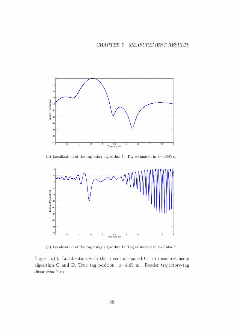
CHAPTER 5. MEASUREMENT RESULTS
3 3.5 4 4.5 5 5.5 6 6.5 7 7.5 8−20
−18
−16
−14
−12
−10
−8
−6
−4
−2
0
Trajectory [m]
Funct
ion P
norm
aliz
ed
(a) Localization of the tag using algorithm C. Tag estimated in x=4.585 m.
3 3.5 4 4.5 5 5.5 6 6.5 7 7.5 8−20
−18
−16
−14
−12
−10
−8
−6
−4
−2
0
Trajectory [m]
Funct
ion P
norm
aliz
ed
(b) Localization of the tag using algorithm D. Tag estimated in x=7.565 m.
Figure 5.13: Localization with the 5 central spaced 0.1 m measures using
algorithm C and D. True tag position: x=4.65 m. Reader trajectory-tag
distance= 2 m.
88
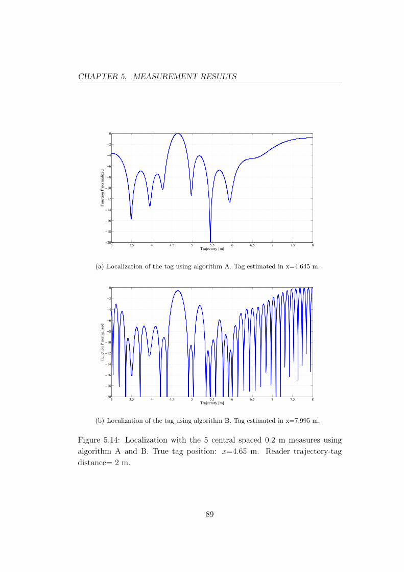
CHAPTER 5. MEASUREMENT RESULTS
3 3.5 4 4.5 5 5.5 6 6.5 7 7.5 8−20
−18
−16
−14
−12
−10
−8
−6
−4
−2
0
Trajectory [m]
Funct
ion P
norm
aliz
ed
(a) Localization of the tag using algorithm A. Tag estimated in x=4.645 m.
3 3.5 4 4.5 5 5.5 6 6.5 7 7.5 8−20
−18
−16
−14
−12
−10
−8
−6
−4
−2
0
Trajectory [m]
Funct
ion P
norm
aliz
ed
(b) Localization of the tag using algorithm B. Tag estimated in x=7.995 m.
Figure 5.14: Localization with the 5 central spaced 0.2 m measures using
algorithm A and B. True tag position: x=4.65 m. Reader trajectory-tag
distance= 2 m.
89
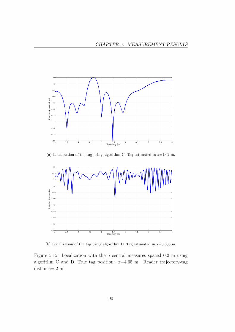
CHAPTER 5. MEASUREMENT RESULTS
3 3.5 4 4.5 5 5.5 6 6.5 7 7.5 8−20
−18
−16
−14
−12
−10
−8
−6
−4
−2
0
Trajectory [m]
Funct
ion P
norm
aliz
ed
(a) Localization of the tag using algorithm C. Tag estimated in x=4.62 m.
3 3.5 4 4.5 5 5.5 6 6.5 7 7.5 8−20
−18
−16
−14
−12
−10
−8
−6
−4
−2
0
Trajectory [m]
Funct
ion P
norm
aliz
ed
(b) Localization of the tag using algorithm D. Tag estimated in x=3.635 m.
Figure 5.15: Localization with the 5 central measures spaced 0.2 m using
algorithm C and D. True tag position: x=4.65 m. Reader trajectory-tag
distance= 2 m.
90
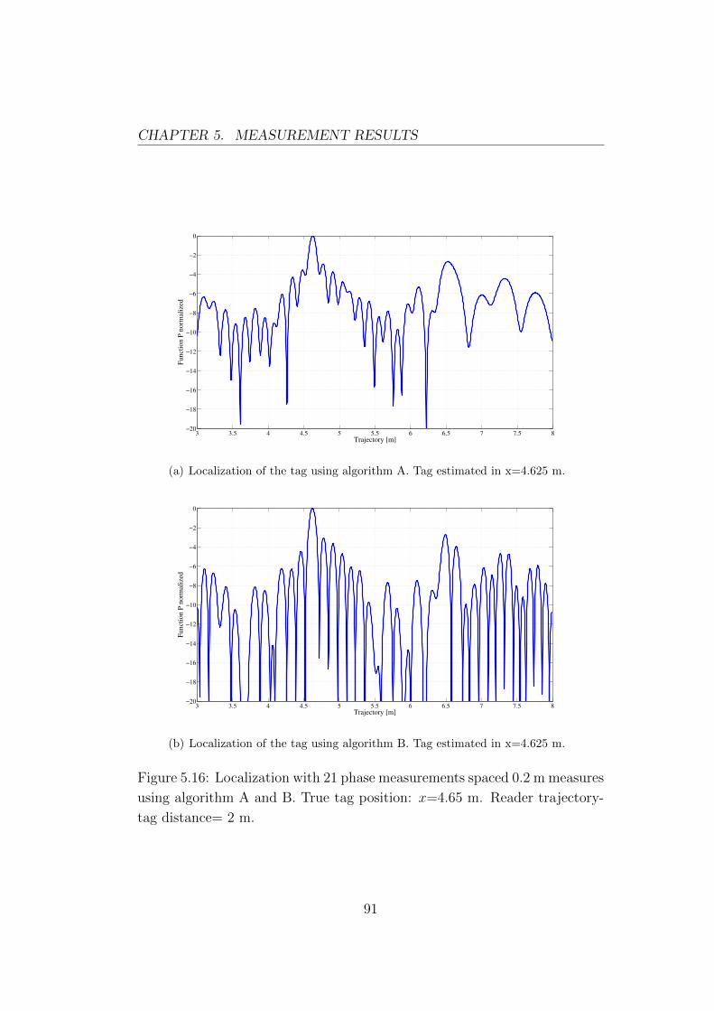
CHAPTER 5. MEASUREMENT RESULTS
3 3.5 4 4.5 5 5.5 6 6.5 7 7.5 8−20
−18
−16
−14
−12
−10
−8
−6
−4
−2
0
Trajectory [m]
Funct
ion P
norm
aliz
ed
(a) Localization of the tag using algorithm A. Tag estimated in x=4.625 m.
3 3.5 4 4.5 5 5.5 6 6.5 7 7.5 8−20
−18
−16
−14
−12
−10
−8
−6
−4
−2
0
Trajectory [m]
Funct
ion P
norm
aliz
ed
(b) Localization of the tag using algorithm B. Tag estimated in x=4.625 m.
Figure 5.16: Localization with 21 phase measurements spaced 0.2 m measures
using algorithm A and B. True tag position: x=4.65 m. Reader trajectory-
tag distance= 2 m.
91
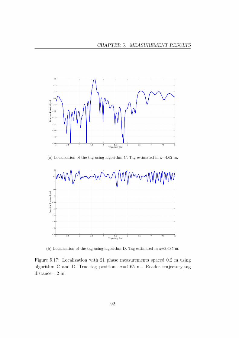
CHAPTER 5. MEASUREMENT RESULTS
3 3.5 4 4.5 5 5.5 6 6.5 7 7.5 8−20
−18
−16
−14
−12
−10
−8
−6
−4
−2
0
Trajectory [m]
Funct
ion P
norm
aliz
ed
(a) Localization of the tag using algorithm C. Tag estimated in x=4.62 m.
3 3.5 4 4.5 5 5.5 6 6.5 7 7.5 8−20
−18
−16
−14
−12
−10
−8
−6
−4
−2
0
Trajectory [m]
Funct
ion P
norm
aliz
ed
(b) Localization of the tag using algorithm D. Tag estimated in x=3.635 m.
Figure 5.17: Localization with 21 phase measurements spaced 0.2 m using
algorithm C and D. True tag position: x=4.65 m. Reader trajectory-tag
distance= 2 m.
92
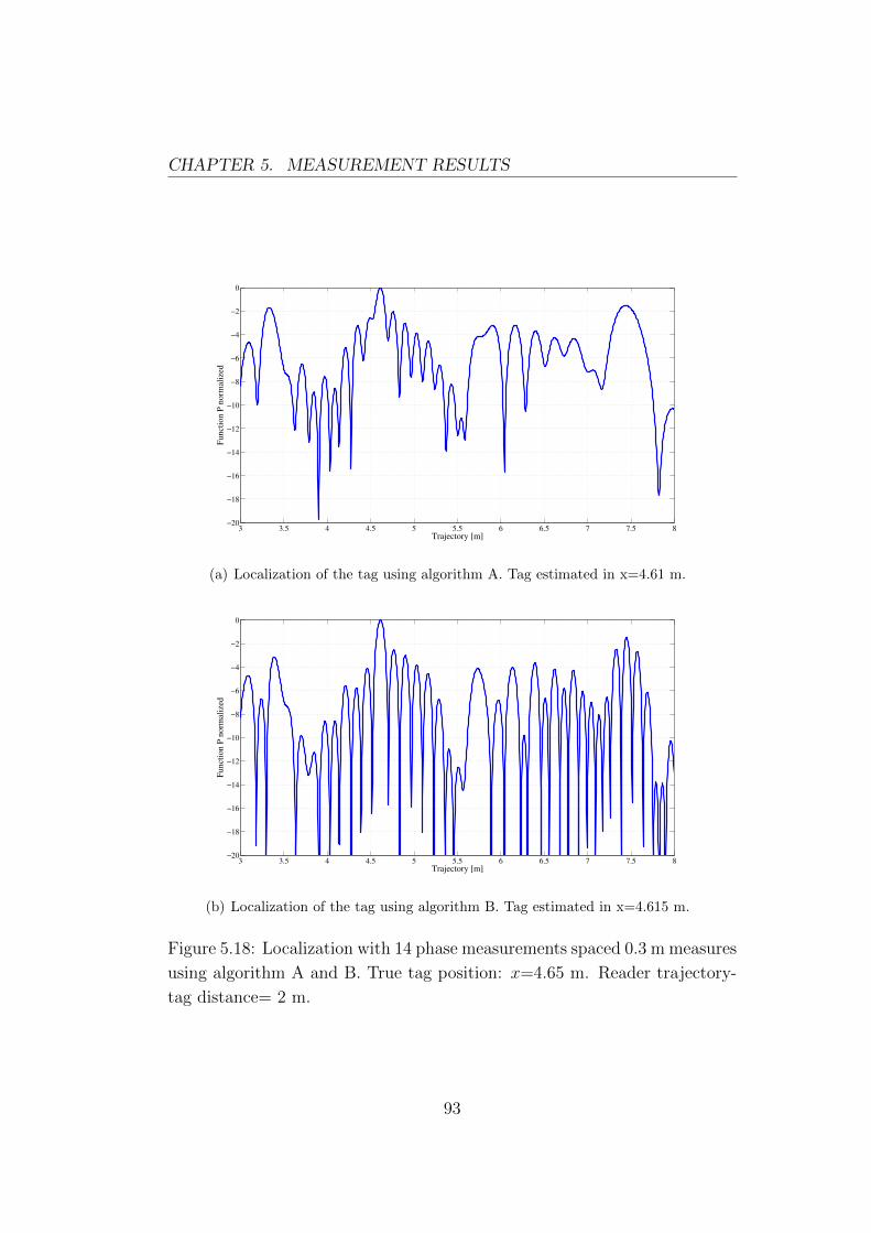
CHAPTER 5. MEASUREMENT RESULTS
3 3.5 4 4.5 5 5.5 6 6.5 7 7.5 8−20
−18
−16
−14
−12
−10
−8
−6
−4
−2
0
Trajectory [m]
Funct
ion P
norm
aliz
ed
(a) Localization of the tag using algorithm A. Tag estimated in x=4.61 m.
3 3.5 4 4.5 5 5.5 6 6.5 7 7.5 8−20
−18
−16
−14
−12
−10
−8
−6
−4
−2
0
Trajectory [m]
Funct
ion P
norm
aliz
ed
(b) Localization of the tag using algorithm B. Tag estimated in x=4.615 m.
Figure 5.18: Localization with 14 phase measurements spaced 0.3 m measures
using algorithm A and B. True tag position: x=4.65 m. Reader trajectory-
tag distance= 2 m.
93
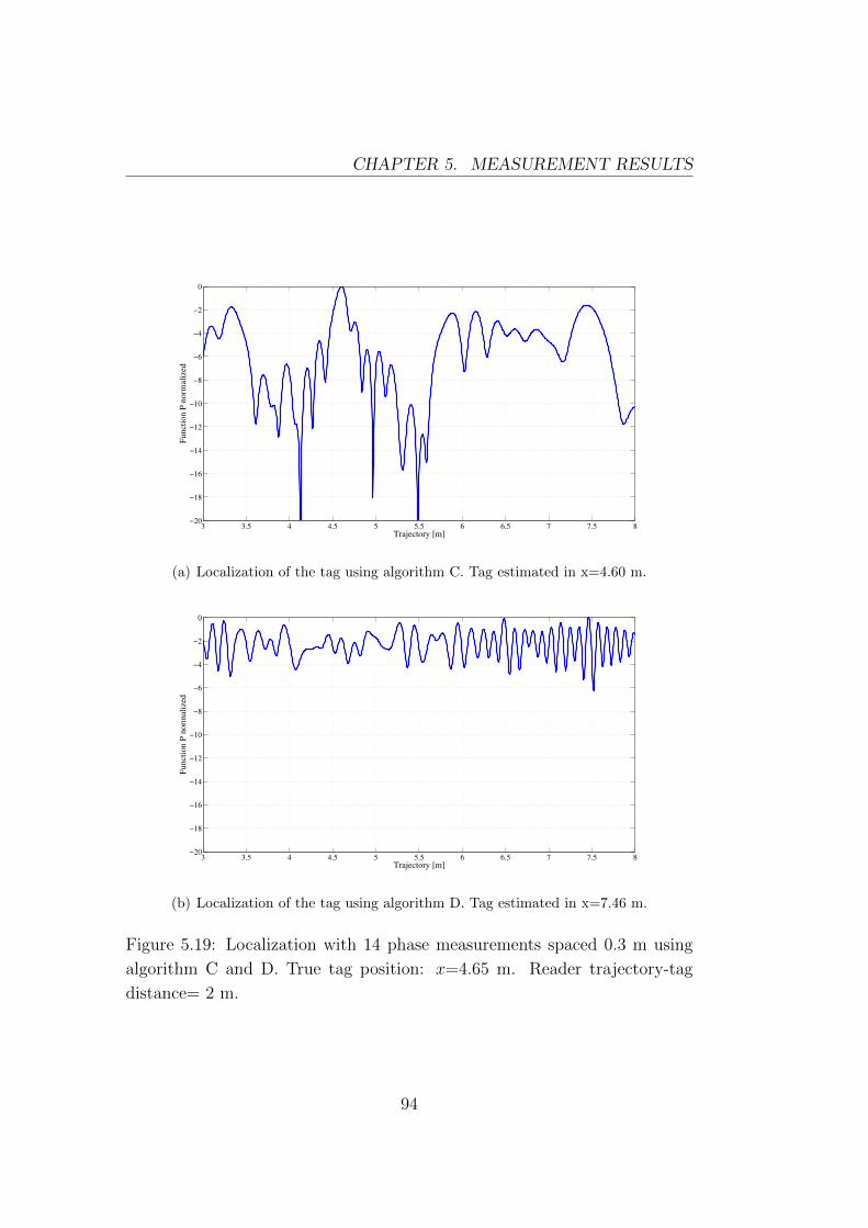
CHAPTER 5. MEASUREMENT RESULTS
3 3.5 4 4.5 5 5.5 6 6.5 7 7.5 8−20
−18
−16
−14
−12
−10
−8
−6
−4
−2
0
Trajectory [m]
Funct
ion P
norm
aliz
ed
(a) Localization of the tag using algorithm C. Tag estimated in x=4.60 m.
3 3.5 4 4.5 5 5.5 6 6.5 7 7.5 8−20
−18
−16
−14
−12
−10
−8
−6
−4
−2
0
Trajectory [m]
Funct
ion P
norm
aliz
ed
(b) Localization of the tag using algorithm D. Tag estimated in x=7.46 m.
Figure 5.19: Localization with 14 phase measurements spaced 0.3 m using
algorithm C and D. True tag position: x=4.65 m. Reader trajectory-tag
distance= 2 m.
94
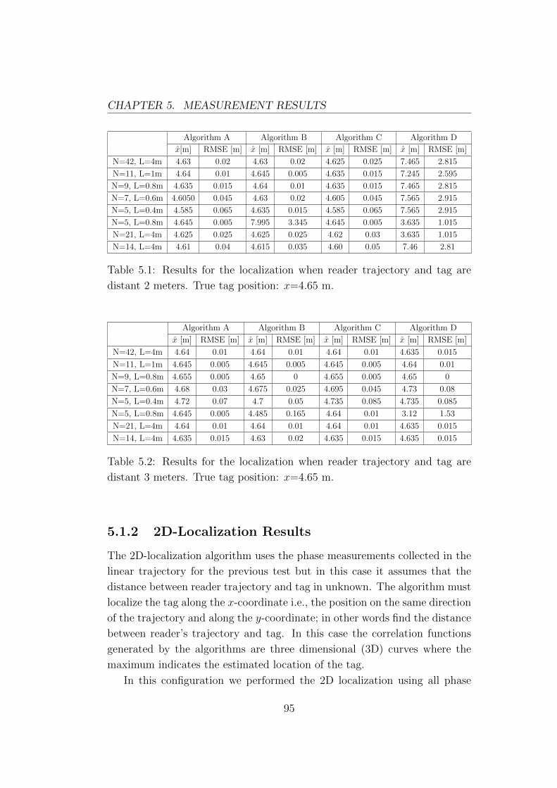
CHAPTER 5. MEASUREMENT RESULTS
Algorithm A Algorithm B Algorithm C Algorithm D
x[m] RMSE [m] x [m] RMSE [m] x [m] RMSE [m] x [m] RMSE [m]
N=42, L=4m 4.63 0.02 4.63 0.02 4.625 0.025 7.465 2.815
N=11, L=1m 4.64 0.01 4.645 0.005 4.635 0.015 7.245 2.595
N=9, L=0.8m 4.635 0.015 4.64 0.01 4.635 0.015 7.465 2.815
N=7, L=0.6m 4.6050 0.045 4.63 0.02 4.605 0.045 7.565 2.915
N=5, L=0.4m 4.585 0.065 4.635 0.015 4.585 0.065 7.565 2.915
N=5, L=0.8m 4.645 0.005 7.995 3.345 4.645 0.005 3.635 1.015
N=21, L=4m 4.625 0.025 4.625 0.025 4.62 0.03 3.635 1.015
N=14, L=4m 4.61 0.04 4.615 0.035 4.60 0.05 7.46 2.81
Table 5.1: Results for the localization when reader trajectory and tag are
distant 2 meters. True tag position: x=4.65 m.
Algorithm A Algorithm B Algorithm C Algorithm D
x [m] RMSE [m] x [m] RMSE [m] x [m] RMSE [m] x [m] RMSE [m]
N=42, L=4m 4.64 0.01 4.64 0.01 4.64 0.01 4.635 0.015
N=11, L=1m 4.645 0.005 4.645 0.005 4.645 0.005 4.64 0.01
N=9, L=0.8m 4.655 0.005 4.65 0 4.655 0.005 4.65 0
N=7, L=0.6m 4.68 0.03 4.675 0.025 4.695 0.045 4.73 0.08
N=5, L=0.4m 4.72 0.07 4.7 0.05 4.735 0.085 4.735 0.085
N=5, L=0.8m 4.645 0.005 4.485 0.165 4.64 0.01 3.12 1.53
N=21, L=4m 4.64 0.01 4.64 0.01 4.64 0.01 4.635 0.015
N=14, L=4m 4.635 0.015 4.63 0.02 4.635 0.015 4.635 0.015
Table 5.2: Results for the localization when reader trajectory and tag are
distant 3 meters. True tag position: x=4.65 m.
5.1.2 2D-Localization Results
The 2D-localization algorithm uses the phase measurements collected in the
linear trajectory for the previous test but in this case it assumes that the
distance between reader trajectory and tag in unknown. The algorithm must
localize the tag along the x-coordinate i.e., the position on the same direction
of the trajectory and along the y-coordinate; in other words find the distance
between reader’s trajectory and tag. In this case the correlation functions
generated by the algorithms are three dimensional (3D) curves where the
maximum indicates the estimated location of the tag.
In this configuration we performed the 2D localization using all phase
95
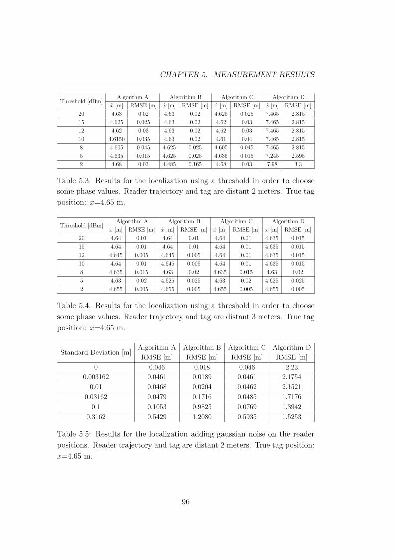
CHAPTER 5. MEASUREMENT RESULTS
Threshold [dBm]Algorithm A Algorithm B Algorithm C Algorithm D
x [m] RMSE [m] x [m] RMSE [m] x [m] RMSE [m] x [m] RMSE [m]
20 4.63 0.02 4.63 0.02 4.625 0.025 7.465 2.815
15 4.625 0.025 4.63 0.02 4.62 0.03 7.465 2.815
12 4.62 0.03 4.63 0.02 4.62 0.03 7.465 2.815
10 4.6150 0.035 4.63 0.02 4.61 0.04 7.465 2.815
8 4.605 0.045 4.625 0.025 4.605 0.045 7.465 2.815
5 4.635 0.015 4.625 0.025 4.635 0.015 7.245 2.595
2 4.68 0.03 4.485 0.165 4.68 0.03 7.98 3.3
Table 5.3: Results for the localization using a threshold in order to choose
some phase values. Reader trajectory and tag are distant 2 meters. True tag
position: x=4.65 m.
Threshold [dBm]Algorithm A Algorithm B Algorithm C Algorithm D
x [m] RMSE [m] x [m] RMSE [m] x [m] RMSE [m] x [m] RMSE [m]
20 4.64 0.01 4.64 0.01 4.64 0.01 4.635 0.015
15 4.64 0.01 4.64 0.01 4.64 0.01 4.635 0.015
12 4.645 0.005 4.645 0.005 4.64 0.01 4.635 0.015
10 4.64 0.01 4.645 0.005 4.64 0.01 4.635 0.015
8 4.635 0.015 4.63 0.02 4.635 0.015 4.63 0.02
5 4.63 0.02 4.625 0.025 4.63 0.02 4.625 0.025
2 4.655 0.005 4.655 0.005 4.655 0.005 4.655 0.005
Table 5.4: Results for the localization using a threshold in order to choose
some phase values. Reader trajectory and tag are distant 3 meters. True tag
position: x=4.65 m.
Standard Deviation [m]Algorithm A Algorithm B Algorithm C Algorithm D
RMSE [m] RMSE [m] RMSE [m] RMSE [m]
0 0.046 0.018 0.046 2.23
0.003162 0.0461 0.0189 0.0461 2.1754
0.01 0.0468 0.0204 0.0462 2.1521
0.03162 0.0479 0.1716 0.0485 1.7176
0.1 0.1053 0.9825 0.0769 1.3942
0.3162 0.5429 1.2080 0.5935 1.5253
Table 5.5: Results for the localization adding gaussian noise on the reader
positions. Reader trajectory and tag are distant 2 meters. True tag position:
x=4.65 m.
96
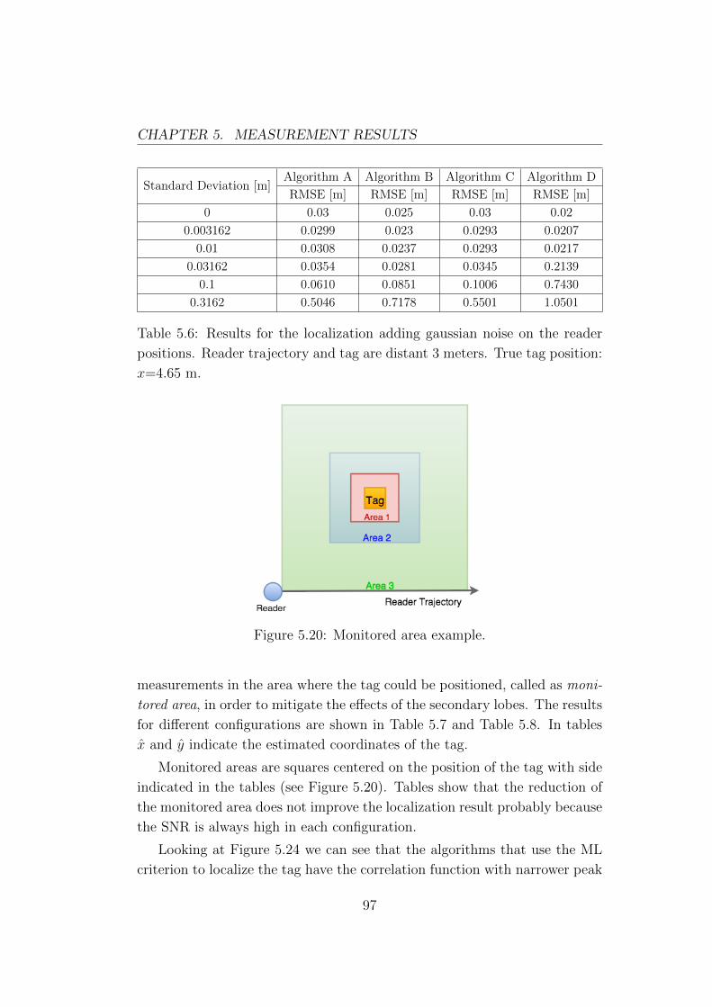
CHAPTER 5. MEASUREMENT RESULTS
Standard Deviation [m]Algorithm A Algorithm B Algorithm C Algorithm D
RMSE [m] RMSE [m] RMSE [m] RMSE [m]
0 0.03 0.025 0.03 0.02
0.003162 0.0299 0.023 0.0293 0.0207
0.01 0.0308 0.0237 0.0293 0.0217
0.03162 0.0354 0.0281 0.0345 0.2139
0.1 0.0610 0.0851 0.1006 0.7430
0.3162 0.5046 0.7178 0.5501 1.0501
Table 5.6: Results for the localization adding gaussian noise on the reader
positions. Reader trajectory and tag are distant 3 meters. True tag position:
x=4.65 m.
Figure 5.20: Monitored area example.
measurements in the area where the tag could be positioned, called as moni-
tored area, in order to mitigate the effects of the secondary lobes. The results
for different configurations are shown in Table 5.7 and Table 5.8. In tables
x and y indicate the estimated coordinates of the tag.
Monitored areas are squares centered on the position of the tag with side
indicated in the tables (see Figure 5.20). Tables show that the reduction of
the monitored area does not improve the localization result probably because
the SNR is always high in each configuration.
Looking at Figure 5.24 we can see that the algorithms that use the ML
criterion to localize the tag have the correlation function with narrower peak
97
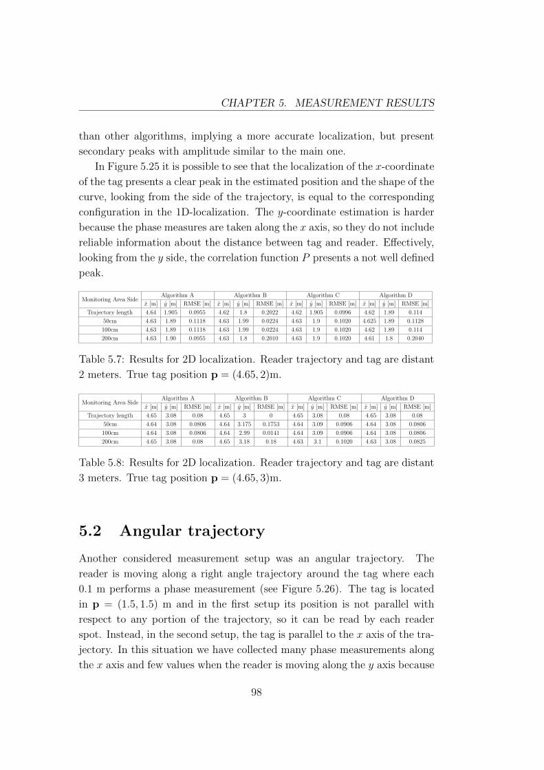
CHAPTER 5. MEASUREMENT RESULTS
than other algorithms, implying a more accurate localization, but present
secondary peaks with amplitude similar to the main one.
In Figure 5.25 it is possible to see that the localization of the x-coordinate
of the tag presents a clear peak in the estimated position and the shape of the
curve, looking from the side of the trajectory, is equal to the corresponding
configuration in the 1D-localization. The y-coordinate estimation is harder
because the phase measures are taken along the x axis, so they do not include
reliable information about the distance between tag and reader. Effectively,
looking from the y side, the correlation function P presents a not well defined
peak.
Monitoring Area SideAlgorithm A Algorithm B Algorithm C Algorithm D
x [m] y [m] RMSE [m] x [m] y [m] RMSE [m] x [m] y [m] RMSE [m] x [m] y [m] RMSE [m]
Trajectory length 4.64 1.905 0.0955 4.62 1.8 0.2022 4.62 1.905 0.0996 4.62 1.89 0.114
50cm 4.63 1.89 0.1118 4.63 1.99 0.0224 4.63 1.9 0.1020 4.625 1.89 0.1128
100cm 4.63 1.89 0.1118 4.63 1.99 0.0224 4.63 1.9 0.1020 4.62 1.89 0.114
200cm 4.63 1.90 0.0955 4.63 1.8 0.2010 4.63 1.9 0.1020 4.61 1.8 0.2040
Table 5.7: Results for 2D localization. Reader trajectory and tag are distant
2 meters. True tag position p = (4.65, 2)m.
Monitoring Area SideAlgorithm A Algorithm B Algorithm C Algorithm D
x [m] y [m] RMSE [m] x [m] y [m] RMSE [m] x [m] y [m] RMSE [m] x [m] y [m] RMSE [m]
Trajectory length 4.65 3.08 0.08 4.65 3 0 4.65 3.08 0.08 4.65 3.08 0.08
50cm 4.64 3.08 0.0806 4.64 3.175 0.1753 4.64 3.09 0.0906 4.64 3.08 0.0806
100cm 4.64 3.08 0.0806 4.64 2.99 0.0141 4.64 3.09 0.0906 4.64 3.08 0.0806
200cm 4.65 3.08 0.08 4.65 3.18 0.18 4.63 3.1 0.1020 4.63 3.08 0.0825
Table 5.8: Results for 2D localization. Reader trajectory and tag are distant
3 meters. True tag position p = (4.65, 3)m.
5.2 Angular trajectory
Another considered measurement setup was an angular trajectory. The
reader is moving along a right angle trajectory around the tag where each
0.1 m performs a phase measurement (see Figure 5.26). The tag is located
in p = (1.5, 1.5) m and in the first setup its position is not parallel with
respect to any portion of the trajectory, so it can be read by each reader
spot. Instead, in the second setup, the tag is parallel to the x axis of the tra-
jectory. In this situation we have collected many phase measurements along
the x axis and few values when the reader is moving along the y axis because
98
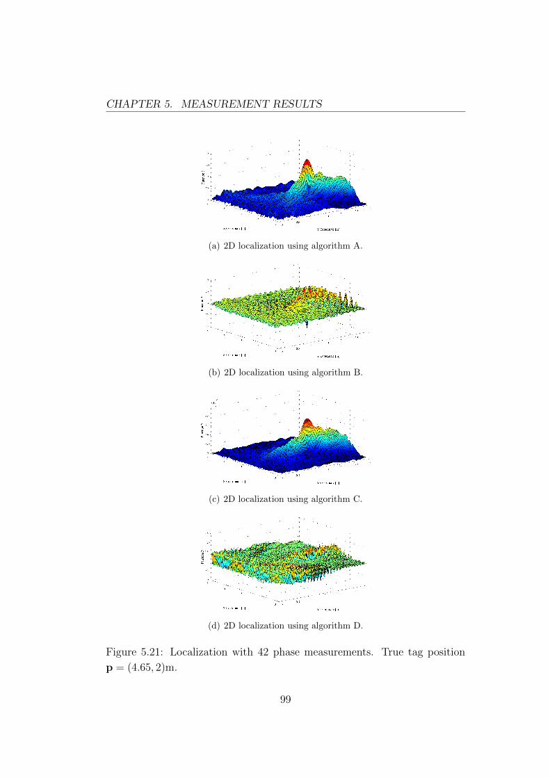
CHAPTER 5. MEASUREMENT RESULTS
(a) 2D localization using algorithm A.
(b) 2D localization using algorithm B.
(c) 2D localization using algorithm C.
(d) 2D localization using algorithm D.
Figure 5.21: Localization with 42 phase measurements. True tag position
p = (4.65, 2)m.
99
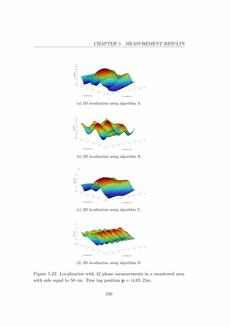
CHAPTER 5. MEASUREMENT RESULTS
1.71.8
1.92
2.12.2
2.32.4
4.4
4.5
4.6
4.7
4.8
4.90
5
10
15
20
25
30
35
40
Y Coordinate [m]X Coordinate [m]
Fu
ncti
on
P
(a) 2D localization using algorithm A.
1.71.8
1.92
2.12.2
2.32.4
4.4
4.5
4.6
4.7
4.8
4.9−40
−30
−20
−10
0
10
20
30
40
Y Coordinate [m]X Coordinate [m]
Fun
cti
on
P
(b) 2D localization using algorithm B.
1.71.8
1.92
2.12.2
2.32.4
4.4
4.5
4.6
4.7
4.8
4.90
0.2
0.4
0.6
0.8
1
x 10−3
Y Coordinate [m]X Coordinate [m]
Fun
cti
on P
(c) 2D localization using algorithm C.
1.71.8
1.92
2.12.2
2.32.4
4.4
4.5
4.6
4.7
4.8
4.90
0.5
1
1.5
2
2.5
Y Coordinate [m]X Coordinate [m]
Fu
ncti
on
P
(d) 2D localization using algorithm D.
Figure 5.22: Localization with 42 phase measurements in a monitored area
with side equal to 50 cm. True tag position p = (4.65, 2)m.
100
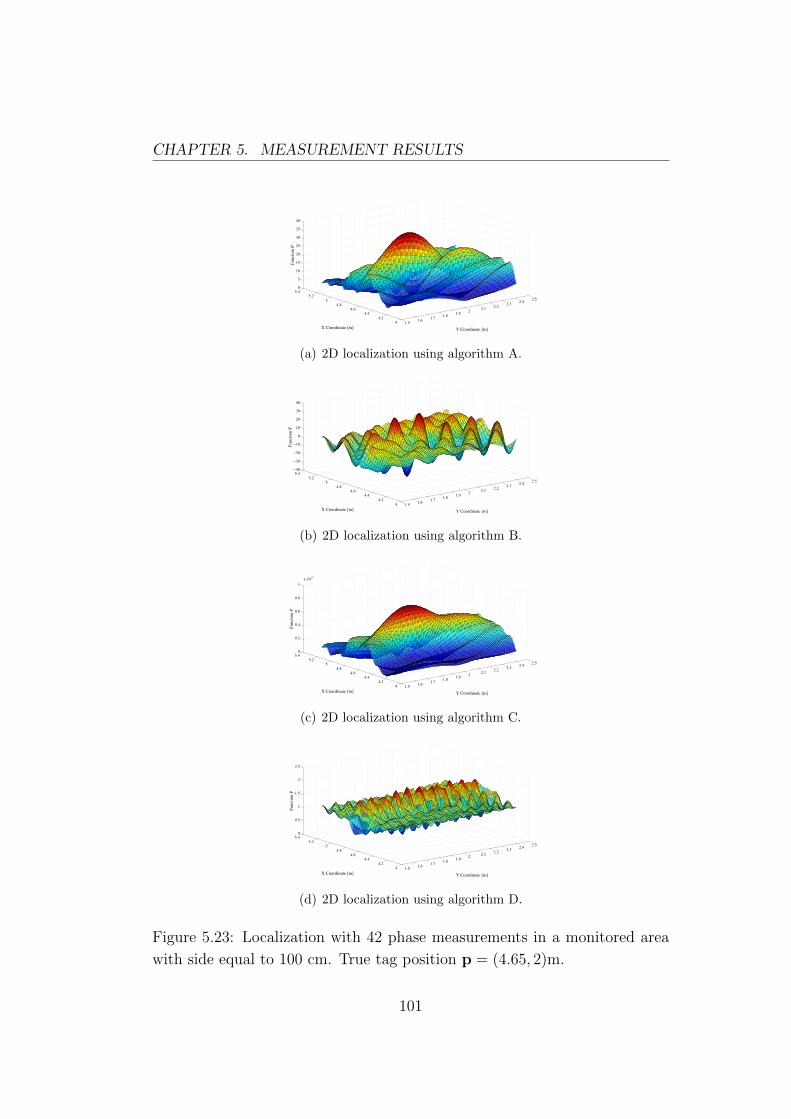
CHAPTER 5. MEASUREMENT RESULTS
1.51.6
1.71.8
1.92
2.12.2
2.32.4
2.5
4
4.2
4.4
4.6
4.8
5
5.2
5.40
5
10
15
20
25
30
35
40
Y Coordinate [m]X Coordinate [m]
Fu
ncti
on
P
(a) 2D localization using algorithm A.
1.51.6
1.71.8
1.92
2.12.2
2.32.4
2.5
4
4.2
4.4
4.6
4.8
5
5.2
5.4−40
−30
−20
−10
0
10
20
30
40
Y Coordinate [m]X Coordinate [m]
Fun
cti
on
P
(b) 2D localization using algorithm B.
1.51.6
1.71.8
1.92
2.12.2
2.32.4
2.5
4
4.2
4.4
4.6
4.8
5
5.2
5.40
0.2
0.4
0.6
0.8
1
x 10−3
Y Coordinate [m]X Coordinate [m]
Fun
cti
on P
(c) 2D localization using algorithm C.
1.51.6
1.71.8
1.92
2.12.2
2.32.4
2.5
4
4.2
4.4
4.6
4.8
5
5.2
5.40
0.5
1
1.5
2
2.5
Y Coordinate [m]X Coordinate [m]
Fu
ncti
on
P
(d) 2D localization using algorithm D.
Figure 5.23: Localization with 42 phase measurements in a monitored area
with side equal to 100 cm. True tag position p = (4.65, 2)m.
101
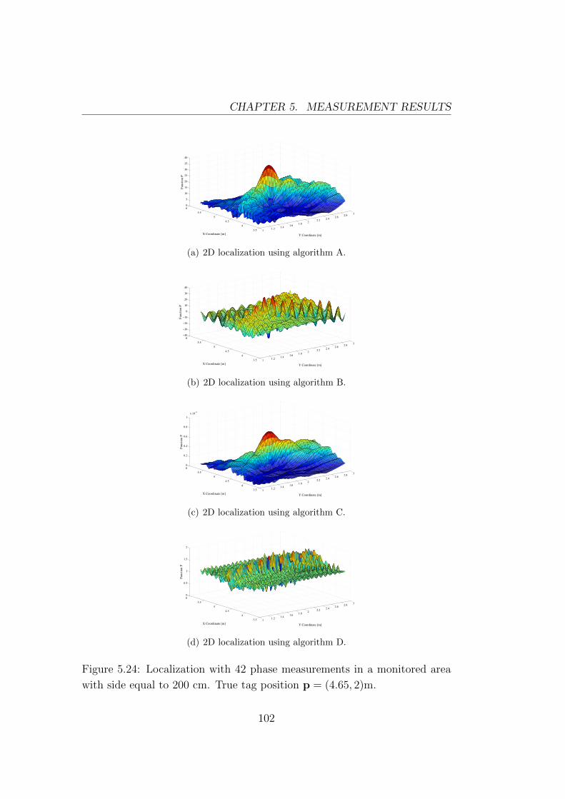
CHAPTER 5. MEASUREMENT RESULTS
11.2
1.41.6
1.82
2.22.4
2.62.8
3
3.5
4
4.5
5
5.5
60
5
10
15
20
25
30
35
40
Y Coordinate [m]X Coordinate [m]
Fu
ncti
on
P
(a) 2D localization using algorithm A.
11.2
1.41.6
1.82
2.22.4
2.62.8
3
3.5
4
4.5
5
5.5
6−40
−30
−20
−10
0
10
20
30
40
Y Coordinate [m]X Coordinate [m]
Fun
cti
on
P
(b) 2D localization using algorithm B.
11.2
1.41.6
1.82
2.22.4
2.62.8
3
3.5
4
4.5
5
5.5
60
0.2
0.4
0.6
0.8
1
x 10−3
Y Coordinate [m]X Coordinate [m]
Fun
cti
on P
(c) 2D localization using algorithm C.
11.2
1.41.6
1.82
2.22.4
2.62.8
3
3.5
4
4.5
5
5.5
60
0.5
1
1.5
2
Y Coordinate [m]X Coordinate [m]
Fu
ncti
on
P
(d) 2D localization using algorithm D.
Figure 5.24: Localization with 42 phase measurements in a monitored area
with side equal to 200 cm. True tag position p = (4.65, 2)m.
102
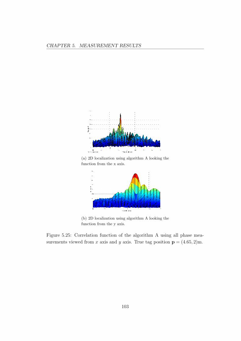
CHAPTER 5. MEASUREMENT RESULTS
(a) 2D localization using algorithm A looking the
function from the x axis.
(b) 2D localization using algorithm A looking the
function from the y axis.
Figure 5.25: Correlation function of the algorithm A using all phase mea-
surements viewed from x axis and y axis. True tag position p = (4.65, 2)m.
103
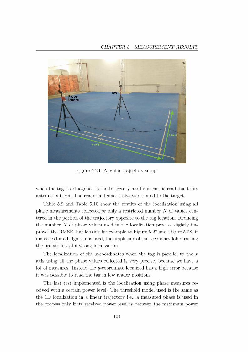
CHAPTER 5. MEASUREMENT RESULTS
Figure 5.26: Angular trajectory setup.
when the tag is orthogonal to the trajectory hardly it can be read due to its
antenna pattern. The reader antenna is always oriented to the target.
Table 5.9 and Table 5.10 show the results of the localization using all
phase measurements collected or only a restricted number N of values cen-
tered in the portion of the trajectory opposite to the tag location. Reducing
the number N of phase values used in the localization process slightly im-
proves the RMSE, but looking for example at Figure 5.27 and Figure 5.28, it
increases for all algorithms used, the amplitude of the secondary lobes raising
the probability of a wrong localization.
The localization of the x-coordinates when the tag is parallel to the x
axis using all the phase values collected is very precise, because we have a
lot of measures. Instead the y-coordinate localized has a high error because
it was possible to read the tag in few reader positions.
The last test implemented is the localization using phase measures re-
ceived with a certain power level. The threshold model used is the same as
the 1D localization in a linear trajectory i.e., a measured phase is used in
the process only if its received power level is between the maximum power
104
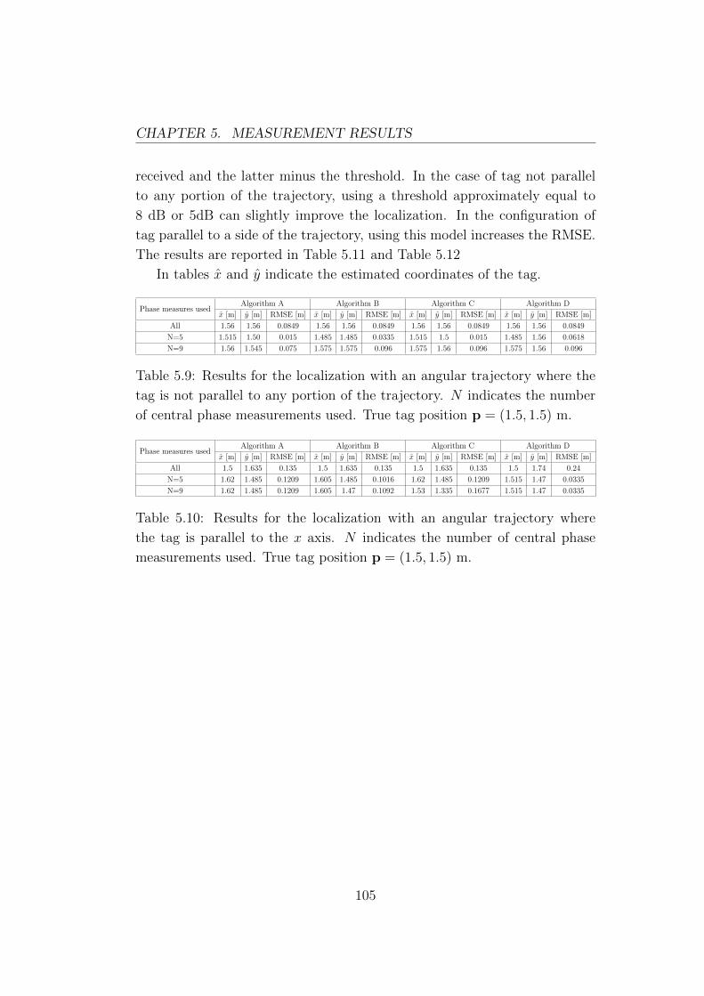
CHAPTER 5. MEASUREMENT RESULTS
received and the latter minus the threshold. In the case of tag not parallel
to any portion of the trajectory, using a threshold approximately equal to
8 dB or 5dB can slightly improve the localization. In the configuration of
tag parallel to a side of the trajectory, using this model increases the RMSE.
The results are reported in Table 5.11 and Table 5.12
In tables x and y indicate the estimated coordinates of the tag.
Phase measures usedAlgorithm A Algorithm B Algorithm C Algorithm D
x [m] y [m] RMSE [m] x [m] y [m] RMSE [m] x [m] y [m] RMSE [m] x [m] y [m] RMSE [m]
All 1.56 1.56 0.0849 1.56 1.56 0.0849 1.56 1.56 0.0849 1.56 1.56 0.0849
N=5 1.515 1.50 0.015 1.485 1.485 0.0335 1.515 1.5 0.015 1.485 1.56 0.0618
N=9 1.56 1.545 0.075 1.575 1.575 0.096 1.575 1.56 0.096 1.575 1.56 0.096
Table 5.9: Results for the localization with an angular trajectory where the
tag is not parallel to any portion of the trajectory. N indicates the number
of central phase measurements used. True tag position p = (1.5, 1.5) m.
Phase measures usedAlgorithm A Algorithm B Algorithm C Algorithm D
x [m] y [m] RMSE [m] x [m] y [m] RMSE [m] x [m] y [m] RMSE [m] x [m] y [m] RMSE [m]
All 1.5 1.635 0.135 1.5 1.635 0.135 1.5 1.635 0.135 1.5 1.74 0.24
N=5 1.62 1.485 0.1209 1.605 1.485 0.1016 1.62 1.485 0.1209 1.515 1.47 0.0335
N=9 1.62 1.485 0.1209 1.605 1.47 0.1092 1.53 1.335 0.1677 1.515 1.47 0.0335
Table 5.10: Results for the localization with an angular trajectory where
the tag is parallel to the x axis. N indicates the number of central phase
measurements used. True tag position p = (1.5, 1.5) m.
105
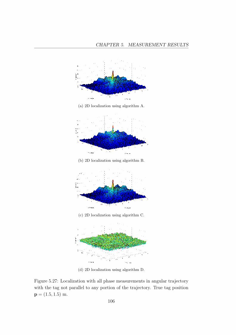
CHAPTER 5. MEASUREMENT RESULTS
(a) 2D localization using algorithm A.
(b) 2D localization using algorithm B.
(c) 2D localization using algorithm C.
(d) 2D localization using algorithm D.
Figure 5.27: Localization with all phase measurements in angular trajectory
with the tag not parallel to any portion of the trajectory. True tag position
p = (1.5, 1.5) m.
106
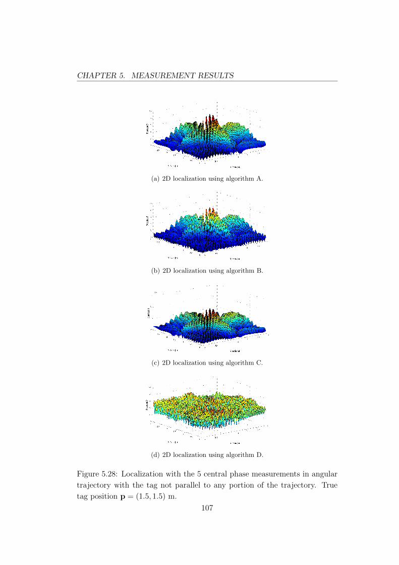
CHAPTER 5. MEASUREMENT RESULTS
(a) 2D localization using algorithm A.
(b) 2D localization using algorithm B.
(c) 2D localization using algorithm C.
(d) 2D localization using algorithm D.
Figure 5.28: Localization with the 5 central phase measurements in angular
trajectory with the tag not parallel to any portion of the trajectory. True
tag position p = (1.5, 1.5) m.
107
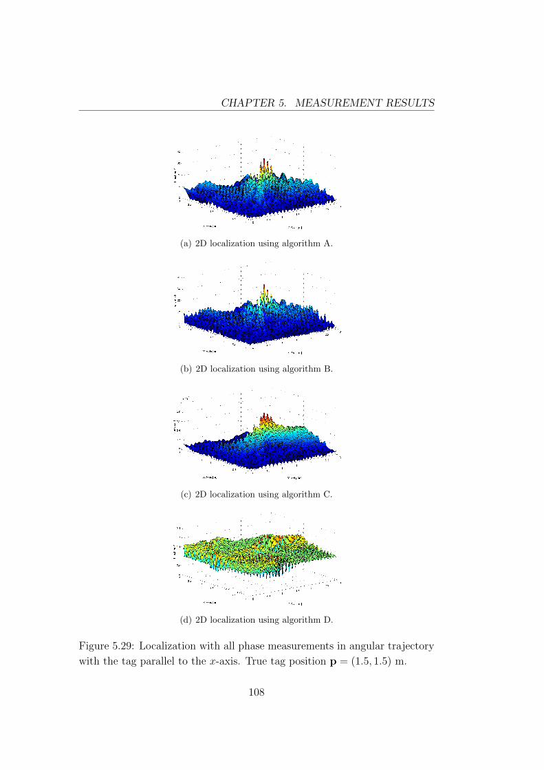
CHAPTER 5. MEASUREMENT RESULTS
(a) 2D localization using algorithm A.
(b) 2D localization using algorithm B.
(c) 2D localization using algorithm C.
(d) 2D localization using algorithm D.
Figure 5.29: Localization with all phase measurements in angular trajectory
with the tag parallel to the x-axis. True tag position p = (1.5, 1.5) m.
108
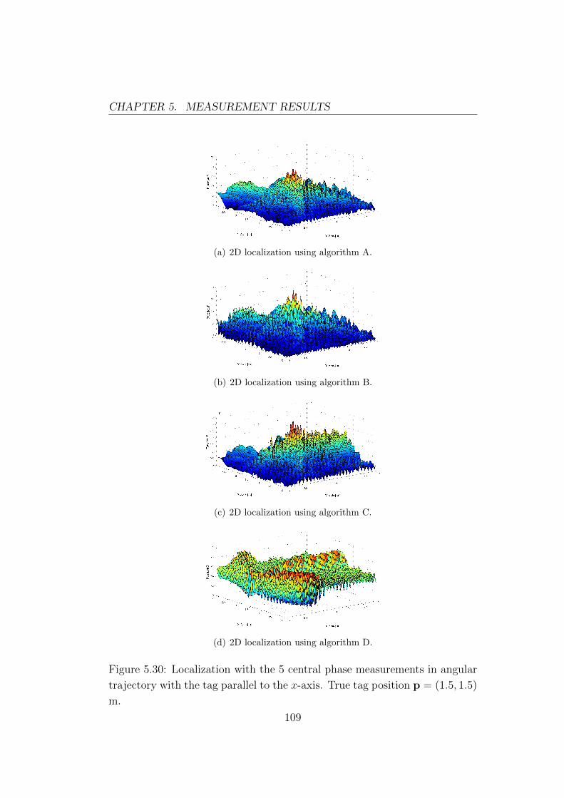
CHAPTER 5. MEASUREMENT RESULTS
(a) 2D localization using algorithm A.
(b) 2D localization using algorithm B.
(c) 2D localization using algorithm C.
(d) 2D localization using algorithm D.
Figure 5.30: Localization with the 5 central phase measurements in angular
trajectory with the tag parallel to the x-axis. True tag position p = (1.5, 1.5)
m.
109
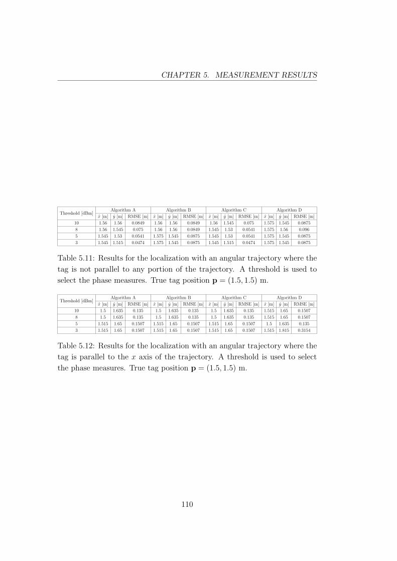
CHAPTER 5. MEASUREMENT RESULTS
Threshold [dBm]Algorithm A Algorithm B Algorithm C Algorithm D
x [m] y [m] RMSE [m] x [m] y [m] RMSE [m] x [m] y [m] RMSE [m] x [m] y [m] RMSE [m]
10 1.56 1.56 0.0849 1.56 1.56 0.0849 1.56 1.545 0.075 1.575 1.545 0.0875
8 1.56 1.545 0.075 1.56 1.56 0.0849 1.545 1.53 0.0541 1.575 1.56 0.096
5 1.545 1.53 0.0541 1.575 1.545 0.0875 1.545 1.53 0.0541 1.575 1.545 0.0875
3 1.545 1.515 0.0474 1.575 1.545 0.0875 1.545 1.515 0.0474 1.575 1.545 0.0875
Table 5.11: Results for the localization with an angular trajectory where the
tag is not parallel to any portion of the trajectory. A threshold is used to
select the phase measures. True tag position p = (1.5, 1.5) m.
Threshold [dBm]Algorithm A Algorithm B Algorithm C Algorithm D
x [m] y [m] RMSE [m] x [m] y [m] RMSE [m] x [m] y [m] RMSE [m] x [m] y [m] RMSE [m]
10 1.5 1.635 0.135 1.5 1.635 0.135 1.5 1.635 0.135 1.515 1.65 0.1507
8 1.5 1.635 0.135 1.5 1.635 0.135 1.5 1.635 0.135 1.515 1.65 0.1507
5 1.515 1.65 0.1507 1.515 1.65 0.1507 1.515 1.65 0.1507 1.5 1.635 0.135
3 1.515 1.65 0.1507 1.515 1.65 0.1507 1.515 1.65 0.1507 1.515 1.815 0.3154
Table 5.12: Results for the localization with an angular trajectory where the
tag is parallel to the x axis of the trajectory. A threshold is used to select
the phase measures. True tag position p = (1.5, 1.5) m.
110
Chapter 6
Conclusions
In this thesis the performance of RFID tag localization with virtual multi-
antenna systems were evaluated. First, the principal RFID phase-based local-
ization techniques present in literature were studied. Then, the ML estimator
for the considered problem was derived.
A Matlab simulator was built in order to evaluate the behavior of the
system and understand the parameters that influence the performance. We
discovered that a reader position not perfectly known can drastically affect
the RMSE of the estimated target location.
Successively, we carried out a measurement campaign in a real indoor
scenario moving the reader on a linear trajectory and on an angular trajec-
tory. Starting from the measurements taken in the two different configura-
tions we applied the algorithms proposed in order to see their differences.
We noticed that there is not a big difference in terms of localization error
between the algorithm derived from the ML criterion and the holographic
localization method proposed in literature. The first presents a correlation
function with a sharper main peak while the second has a smoother function.
This means that the ML criterion has a higher accuracy. This method also
presents secondary lobes with amplitude higher than the holographic local-
ization method. This increases the possibility of a wrong localization due
to ambiguity problems, which leads to outliers generated by high secondary
lobes.
Moreover, we discovered that the information about the RSS of the single
phase measures used in the localization process does not always improve the
performance.
111

CHAPTER 6. CONCLUSIONS
The resultant accuracy of the algorithms is on average equal to few cen-
timeters; in the worst cases seen the RMSE of the localization is always less
than 0.2 m.
Future developments of this work could consider the testing of the algo-
rithms using a real time automatic system in an environment with many tags
that can collect many phase measurements and accurate odometers to mea-
sure the distance between consecutive reader positions. Another research
aspect to be addressed could consider efficient methods for estimating the
relative distance of unknown tags with respect to reference tags present in
the environment.
112
Appendix A
1D-Localization Results
This appendix shows the results obtained with 1D-localization when reader
trajectory and tag distance is equal to 3 meter.
113
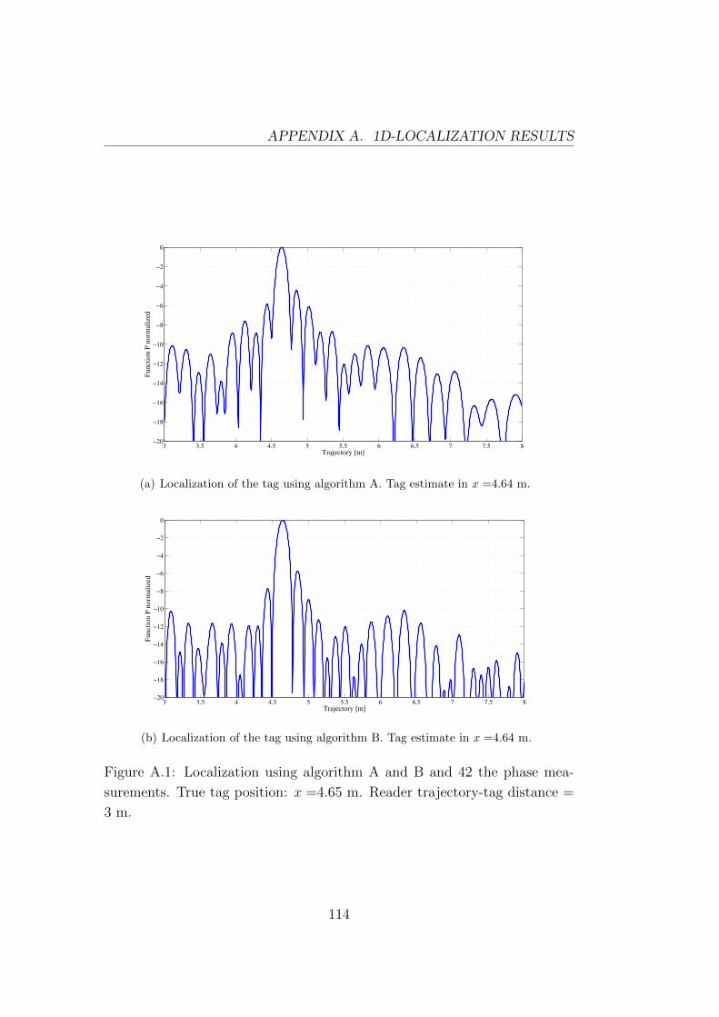
APPENDIX A. 1D-LOCALIZATION RESULTS
3 3.5 4 4.5 5 5.5 6 6.5 7 7.5 8−20
−18
−16
−14
−12
−10
−8
−6
−4
−2
0
Trajectory [m]
Funct
ion P
norm
aliz
ed
(a) Localization of the tag using algorithm A. Tag estimate in x =4.64 m.
3 3.5 4 4.5 5 5.5 6 6.5 7 7.5 8−20
−18
−16
−14
−12
−10
−8
−6
−4
−2
0
Trajectory [m]
Funct
ion P
norm
aliz
ed
(b) Localization of the tag using algorithm B. Tag estimate in x =4.64 m.
Figure A.1: Localization using algorithm A and B and 42 the phase mea-
surements. True tag position: x =4.65 m. Reader trajectory-tag distance =
3 m.
114
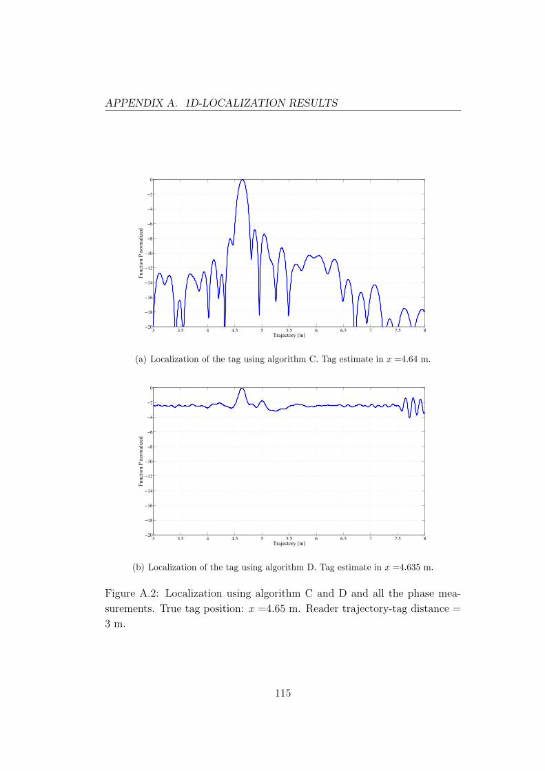
APPENDIX A. 1D-LOCALIZATION RESULTS
3 3.5 4 4.5 5 5.5 6 6.5 7 7.5 8−20
−18
−16
−14
−12
−10
−8
−6
−4
−2
0
Trajectory [m]
Funct
ion P
norm
aliz
ed
(a) Localization of the tag using algorithm C. Tag estimate in x =4.64 m.
3 3.5 4 4.5 5 5.5 6 6.5 7 7.5 8−20
−18
−16
−14
−12
−10
−8
−6
−4
−2
0
Trajectory [m]
Funct
ion P
norm
aliz
ed
(b) Localization of the tag using algorithm D. Tag estimate in x =4.635 m.
Figure A.2: Localization using algorithm C and D and all the phase mea-
surements. True tag position: x =4.65 m. Reader trajectory-tag distance =
3 m.
115
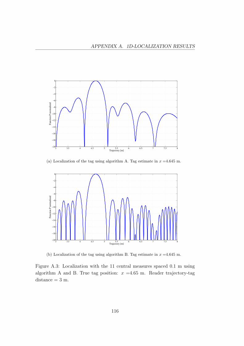
APPENDIX A. 1D-LOCALIZATION RESULTS
3 3.5 4 4.5 5 5.5 6 6.5 7 7.5 8−20
−18
−16
−14
−12
−10
−8
−6
−4
−2
0
Trajectory [m]
Funct
ion P
norm
aliz
ed
(a) Localization of the tag using algorithm A. Tag estimate in x =4.645 m.
3 3.5 4 4.5 5 5.5 6 6.5 7 7.5 8−20
−18
−16
−14
−12
−10
−8
−6
−4
−2
0
Trajectory [m]
Funct
ion P
norm
aliz
ed
(b) Localization of the tag using algorithm B. Tag estimate in x =4.645 m.
Figure A.3: Localization with the 11 central measures spaced 0.1 m using
algorithm A and B. True tag position: x =4.65 m. Reader trajectory-tag
distance = 3 m.
116
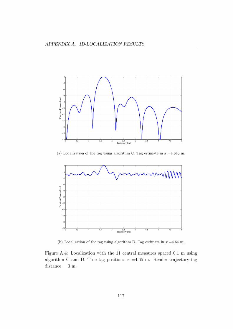
APPENDIX A. 1D-LOCALIZATION RESULTS
3 3.5 4 4.5 5 5.5 6 6.5 7 7.5 8−20
−18
−16
−14
−12
−10
−8
−6
−4
−2
0
Trajectory [m]
Funct
ion P
norm
aliz
ed
(a) Localization of the tag using algorithm C. Tag estimate in x =4.645 m.
3 3.5 4 4.5 5 5.5 6 6.5 7 7.5 8−20
−18
−16
−14
−12
−10
−8
−6
−4
−2
0
Trajectory [m]
Funct
ion P
norm
aliz
ed
(b) Localization of the tag using algorithm D. Tag estimate in x =4.64 m.
Figure A.4: Localization with the 11 central measures spaced 0.1 m using
algorithm C and D. True tag position: x =4.65 m. Reader trajectory-tag
distance = 3 m.
117
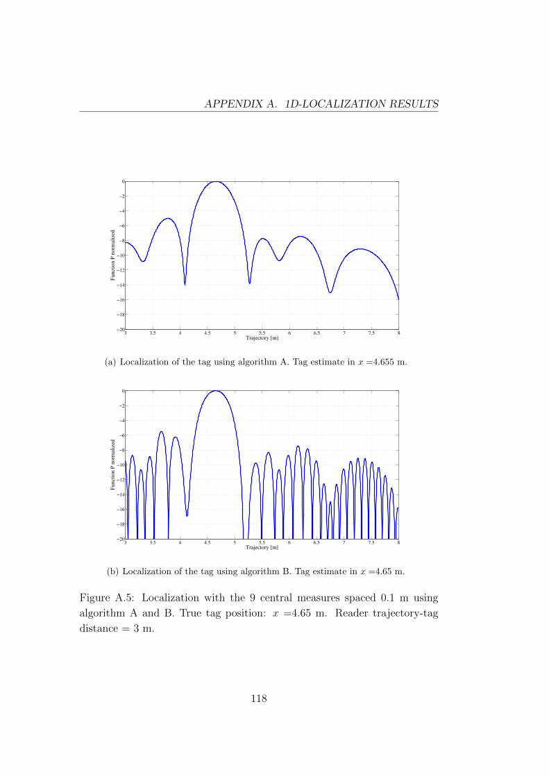
APPENDIX A. 1D-LOCALIZATION RESULTS
3 3.5 4 4.5 5 5.5 6 6.5 7 7.5 8−20
−18
−16
−14
−12
−10
−8
−6
−4
−2
0
Trajectory [m]
Funct
ion P
norm
aliz
ed
(a) Localization of the tag using algorithm A. Tag estimate in x =4.655 m.
3 3.5 4 4.5 5 5.5 6 6.5 7 7.5 8−20
−18
−16
−14
−12
−10
−8
−6
−4
−2
0
Trajectory [m]
Funct
ion P
norm
aliz
ed
(b) Localization of the tag using algorithm B. Tag estimate in x =4.65 m.
Figure A.5: Localization with the 9 central measures spaced 0.1 m using
algorithm A and B. True tag position: x =4.65 m. Reader trajectory-tag
distance = 3 m.
118
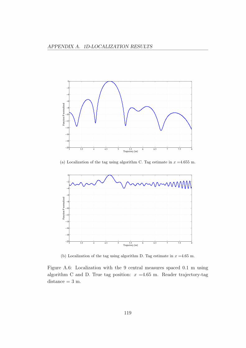
APPENDIX A. 1D-LOCALIZATION RESULTS
3 3.5 4 4.5 5 5.5 6 6.5 7 7.5 8−20
−18
−16
−14
−12
−10
−8
−6
−4
−2
0
Trajectory [m]
Funct
ion P
norm
aliz
ed
(a) Localization of the tag using algorithm C. Tag estimate in x =4.655 m.
3 3.5 4 4.5 5 5.5 6 6.5 7 7.5 8−20
−18
−16
−14
−12
−10
−8
−6
−4
−2
0
Trajectory [m]
Funct
ion P
norm
aliz
ed
(b) Localization of the tag using algorithm D. Tag estimate in x =4.65 m.
Figure A.6: Localization with the 9 central measures spaced 0.1 m using
algorithm C and D. True tag position: x =4.65 m. Reader trajectory-tag
distance = 3 m.
119
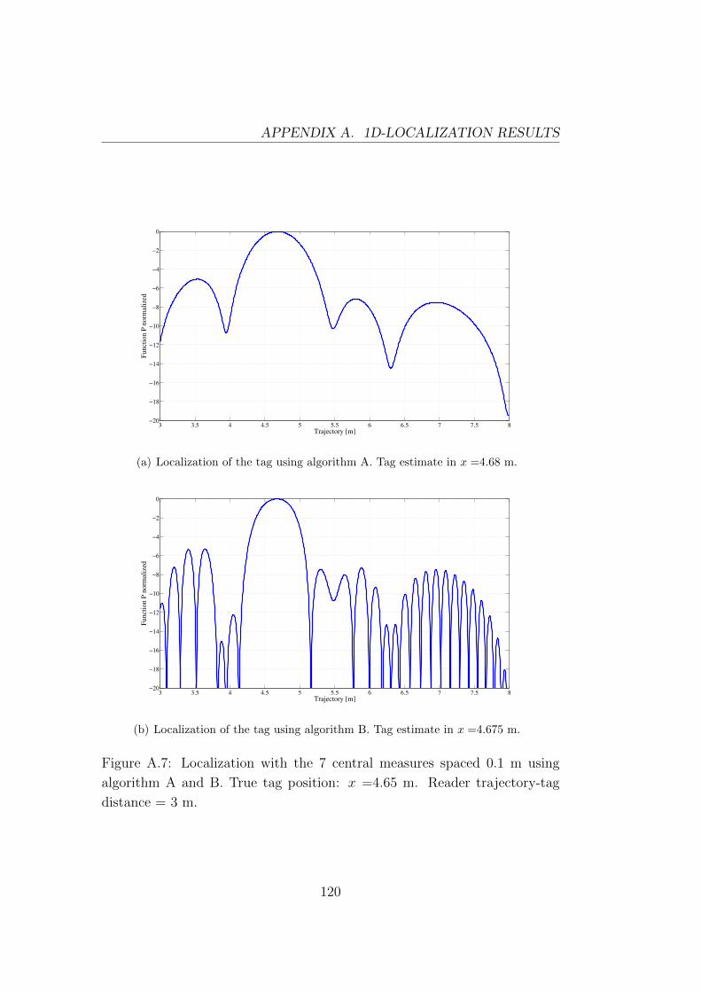
APPENDIX A. 1D-LOCALIZATION RESULTS
3 3.5 4 4.5 5 5.5 6 6.5 7 7.5 8−20
−18
−16
−14
−12
−10
−8
−6
−4
−2
0
Trajectory [m]
Funct
ion P
norm
aliz
ed
(a) Localization of the tag using algorithm A. Tag estimate in x =4.68 m.
3 3.5 4 4.5 5 5.5 6 6.5 7 7.5 8−20
−18
−16
−14
−12
−10
−8
−6
−4
−2
0
Trajectory [m]
Funct
ion P
norm
aliz
ed
(b) Localization of the tag using algorithm B. Tag estimate in x =4.675 m.
Figure A.7: Localization with the 7 central measures spaced 0.1 m using
algorithm A and B. True tag position: x =4.65 m. Reader trajectory-tag
distance = 3 m.
120
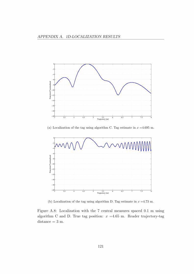
APPENDIX A. 1D-LOCALIZATION RESULTS
3 3.5 4 4.5 5 5.5 6 6.5 7 7.5 8−20
−18
−16
−14
−12
−10
−8
−6
−4
−2
0
Trajectory [m]
Funct
ion P
norm
aliz
ed
(a) Localization of the tag using algorithm C. Tag estimate in x =4.695 m.
3 3.5 4 4.5 5 5.5 6 6.5 7 7.5 8−20
−18
−16
−14
−12
−10
−8
−6
−4
−2
0
Trajectory [m]
Funct
ion P
norm
aliz
ed
(b) Localization of the tag using algorithm D. Tag estimate in x =4.73 m.
Figure A.8: Localization with the 7 central measures spaced 0.1 m using
algorithm C and D. True tag position: x =4.65 m. Reader trajectory-tag
distance = 3 m.
121
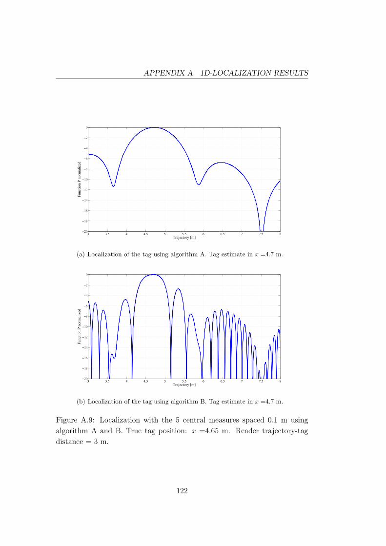
APPENDIX A. 1D-LOCALIZATION RESULTS
3 3.5 4 4.5 5 5.5 6 6.5 7 7.5 8−20
−18
−16
−14
−12
−10
−8
−6
−4
−2
0
Trajectory [m]
Funct
ion P
norm
aliz
ed
(a) Localization of the tag using algorithm A. Tag estimate in x =4.7 m.
3 3.5 4 4.5 5 5.5 6 6.5 7 7.5 8−20
−18
−16
−14
−12
−10
−8
−6
−4
−2
0
Trajectory [m]
Funct
ion P
norm
aliz
ed
(b) Localization of the tag using algorithm B. Tag estimate in x =4.7 m.
Figure A.9: Localization with the 5 central measures spaced 0.1 m using
algorithm A and B. True tag position: x =4.65 m. Reader trajectory-tag
distance = 3 m.
122
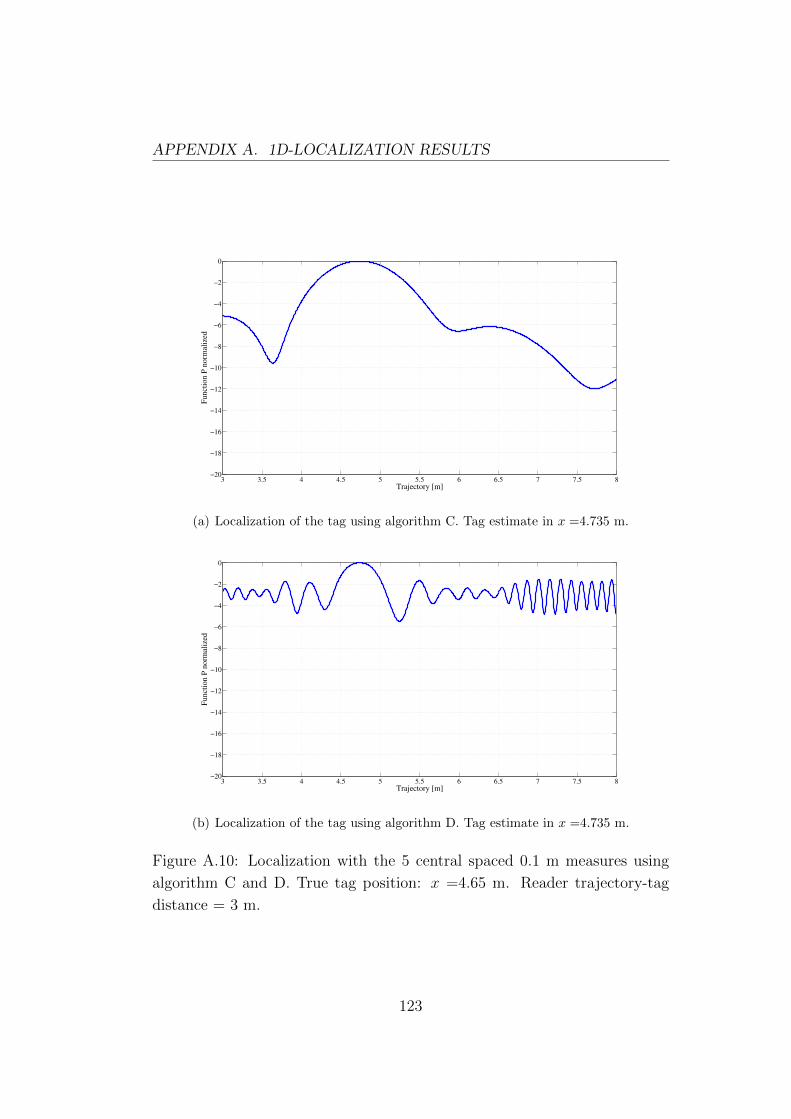
APPENDIX A. 1D-LOCALIZATION RESULTS
3 3.5 4 4.5 5 5.5 6 6.5 7 7.5 8−20
−18
−16
−14
−12
−10
−8
−6
−4
−2
0
Trajectory [m]
Funct
ion P
norm
aliz
ed
(a) Localization of the tag using algorithm C. Tag estimate in x =4.735 m.
3 3.5 4 4.5 5 5.5 6 6.5 7 7.5 8−20
−18
−16
−14
−12
−10
−8
−6
−4
−2
0
Trajectory [m]
Funct
ion P
norm
aliz
ed
(b) Localization of the tag using algorithm D. Tag estimate in x =4.735 m.
Figure A.10: Localization with the 5 central spaced 0.1 m measures using
algorithm C and D. True tag position: x =4.65 m. Reader trajectory-tag
distance = 3 m.
123
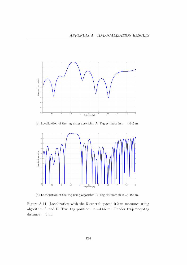
APPENDIX A. 1D-LOCALIZATION RESULTS
3 3.5 4 4.5 5 5.5 6 6.5 7 7.5 8−20
−18
−16
−14
−12
−10
−8
−6
−4
−2
0
Trajectory [m]
Funct
ion P
norm
aliz
ed
(a) Localization of the tag using algorithm A. Tag estimate in x =4.645 m.
3 3.5 4 4.5 5 5.5 6 6.5 7 7.5 8−20
−18
−16
−14
−12
−10
−8
−6
−4
−2
0
Trajectory [m]
Funct
ion P
norm
aliz
ed
(b) Localization of the tag using algorithm B. Tag estimate in x =4.485 m.
Figure A.11: Localization with the 5 central spaced 0.2 m measures using
algorithm A and B. True tag position: x =4.65 m. Reader trajectory-tag
distance = 3 m.
124
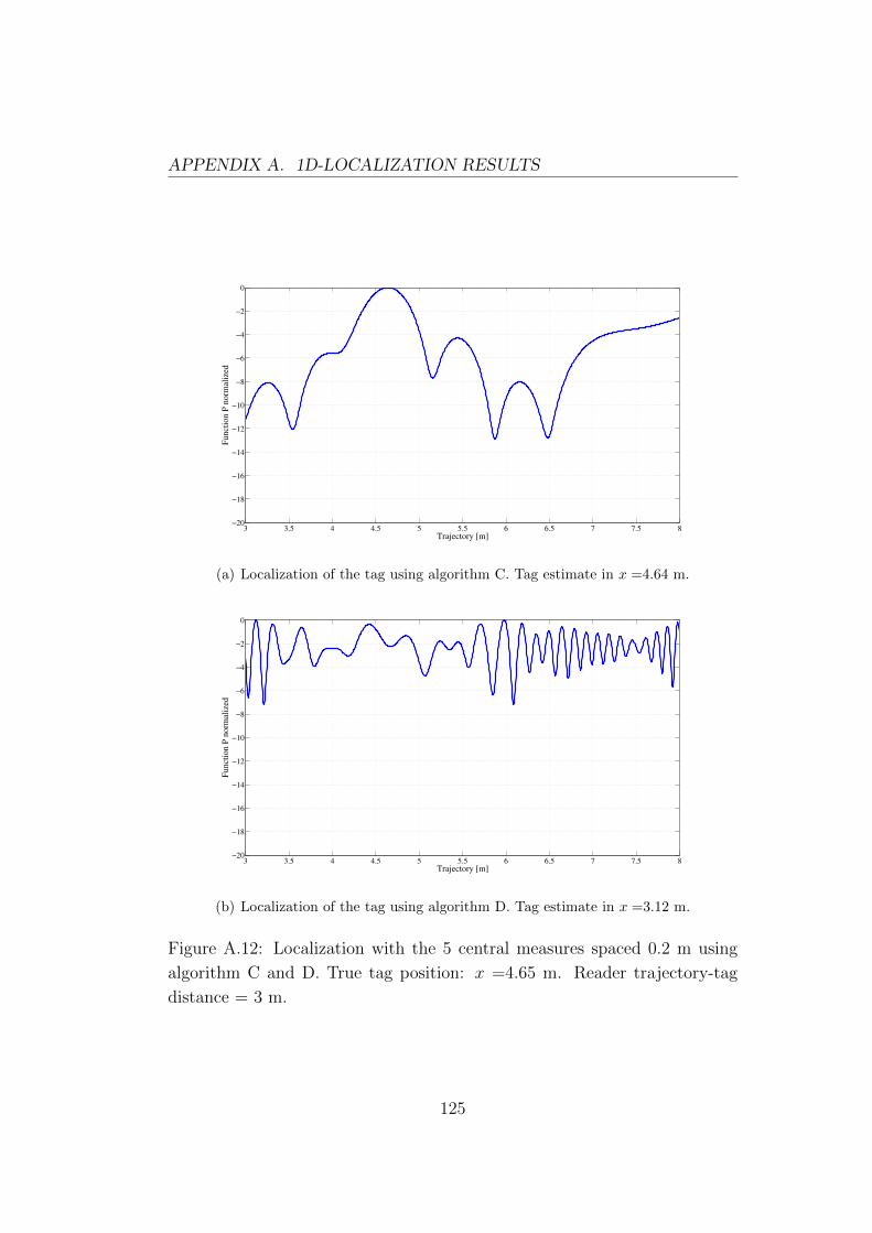
APPENDIX A. 1D-LOCALIZATION RESULTS
3 3.5 4 4.5 5 5.5 6 6.5 7 7.5 8−20
−18
−16
−14
−12
−10
−8
−6
−4
−2
0
Trajectory [m]
Funct
ion P
norm
aliz
ed
(a) Localization of the tag using algorithm C. Tag estimate in x =4.64 m.
3 3.5 4 4.5 5 5.5 6 6.5 7 7.5 8−20
−18
−16
−14
−12
−10
−8
−6
−4
−2
0
Trajectory [m]
Funct
ion P
norm
aliz
ed
(b) Localization of the tag using algorithm D. Tag estimate in x =3.12 m.
Figure A.12: Localization with the 5 central measures spaced 0.2 m using
algorithm C and D. True tag position: x =4.65 m. Reader trajectory-tag
distance = 3 m.
125
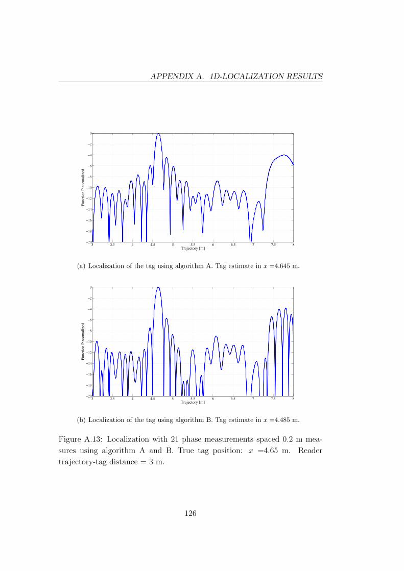
APPENDIX A. 1D-LOCALIZATION RESULTS
3 3.5 4 4.5 5 5.5 6 6.5 7 7.5 8−20
−18
−16
−14
−12
−10
−8
−6
−4
−2
0
Trajectory [m]
Funct
ion P
norm
aliz
ed
(a) Localization of the tag using algorithm A. Tag estimate in x =4.645 m.
3 3.5 4 4.5 5 5.5 6 6.5 7 7.5 8−20
−18
−16
−14
−12
−10
−8
−6
−4
−2
0
Trajectory [m]
Funct
ion P
norm
aliz
ed
(b) Localization of the tag using algorithm B. Tag estimate in x =4.485 m.
Figure A.13: Localization with 21 phase measurements spaced 0.2 m mea-
sures using algorithm A and B. True tag position: x =4.65 m. Reader
trajectory-tag distance = 3 m.
126
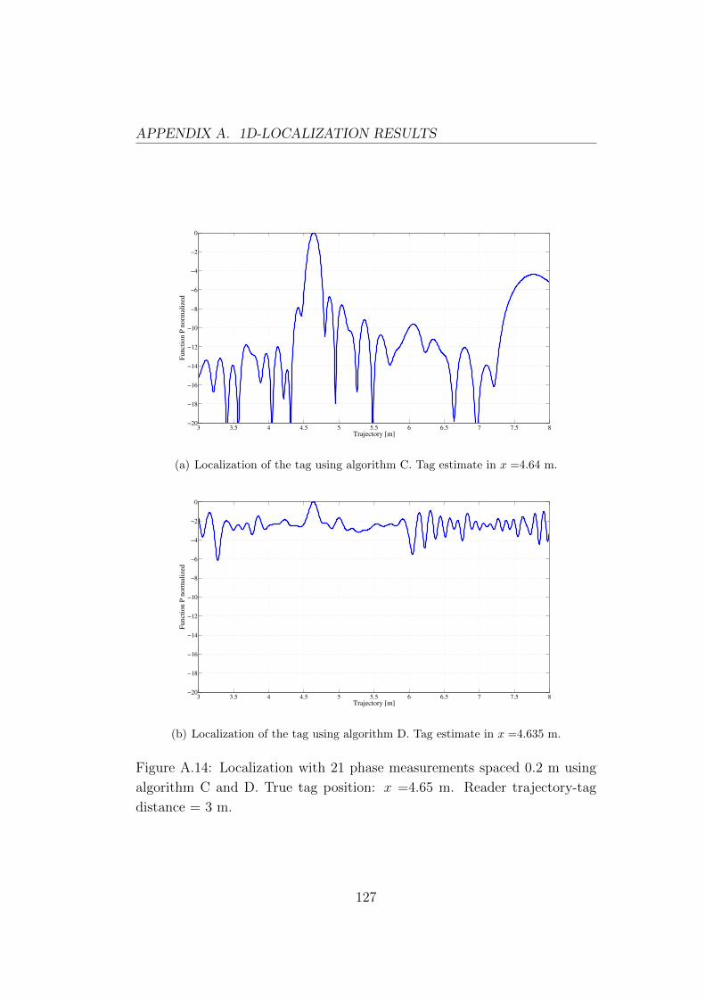
APPENDIX A. 1D-LOCALIZATION RESULTS
3 3.5 4 4.5 5 5.5 6 6.5 7 7.5 8−20
−18
−16
−14
−12
−10
−8
−6
−4
−2
0
Trajectory [m]
Funct
ion P
norm
aliz
ed
(a) Localization of the tag using algorithm C. Tag estimate in x =4.64 m.
3 3.5 4 4.5 5 5.5 6 6.5 7 7.5 8−20
−18
−16
−14
−12
−10
−8
−6
−4
−2
0
Trajectory [m]
Funct
ion P
norm
aliz
ed
(b) Localization of the tag using algorithm D. Tag estimate in x =4.635 m.
Figure A.14: Localization with 21 phase measurements spaced 0.2 m using
algorithm C and D. True tag position: x =4.65 m. Reader trajectory-tag
distance = 3 m.
127
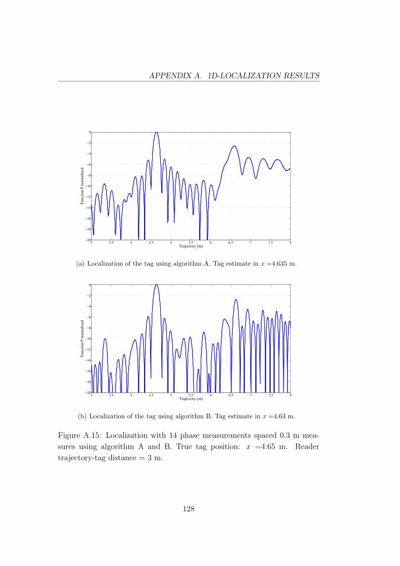
APPENDIX A. 1D-LOCALIZATION RESULTS
3 3.5 4 4.5 5 5.5 6 6.5 7 7.5 8−20
−18
−16
−14
−12
−10
−8
−6
−4
−2
0
Trajectory [m]
Funct
ion P
norm
aliz
ed
(a) Localization of the tag using algorithm A. Tag estimate in x =4.635 m.
3 3.5 4 4.5 5 5.5 6 6.5 7 7.5 8−20
−18
−16
−14
−12
−10
−8
−6
−4
−2
0
Trajectory [m]
Funct
ion P
norm
aliz
ed
(b) Localization of the tag using algorithm B. Tag estimate in x =4.63 m.
Figure A.15: Localization with 14 phase measurements spaced 0.3 m mea-
sures using algorithm A and B. True tag position: x =4.65 m. Reader
trajectory-tag distance = 3 m.
128
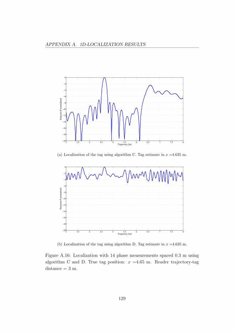
APPENDIX A. 1D-LOCALIZATION RESULTS
3 3.5 4 4.5 5 5.5 6 6.5 7 7.5 8−20
−18
−16
−14
−12
−10
−8
−6
−4
−2
0
Trajectory [m]
Funct
ion P
norm
aliz
ed
(a) Localization of the tag using algorithm C. Tag estimate in x =4.635 m.
3 3.5 4 4.5 5 5.5 6 6.5 7 7.5 8−20
−18
−16
−14
−12
−10
−8
−6
−4
−2
0
Trajectory [m]
Funct
ion P
norm
aliz
ed
(b) Localization of the tag using algorithm D. Tag estimate in x =4.635 m.
Figure A.16: Localization with 14 phase measurements spaced 0.3 m using
algorithm C and D. True tag position: x =4.65 m. Reader trajectory-tag
distance = 3 m.
129

APPENDIX A. 1D-LOCALIZATION RESULTS
130

Acknowledgments
Prima di tutti vorrei ringraziare il Prof. Davide Dardari e il Dott. Nicolo De-
carli per avermi dato la possibilita di lavorare a questo interessante progetto,
per avermi aiutato e dato preziosi consigli durante tutto questo periodo di
tesi.
Vorrei ringraziare tutta la mia famiglia per avermi supportato e soppor-
tato durante questi ultimi anni, per avermi dato la possibilita di studiare
serenamente e per non avermi mai fatto mancare nulla.
Infine un caloroso ringraziamento va agli amici di sempre, a tutti i com-
pagni di corso che mi hanno accompagnato durante questo percorso e a tutte
le persone incontrate durante questi ultimi 5 anni.
131

132
List of Tables
4.1 Main features of Impinj Speedway Revolution R420 [37]. . . . 54
4.2 Nominal read range of tags for transmitted power of 1W. . . . 65
5.1 Results for the localization when reader trajectory and tag are
distant 2 meters. True tag position: x=4.65 m. . . . . . . . . 95
5.2 Results for the localization when reader trajectory and tag are
distant 3 meters. True tag position: x=4.65 m. . . . . . . . . 95
5.3 Results for the localization using a threshold in order to choose
some phase values. Reader trajectory and tag are distant 2
meters. True tag position: x=4.65 m. . . . . . . . . . . . . . . 96
5.4 Results for the localization using a threshold in order to choose
some phase values. Reader trajectory and tag are distant 3
meters. True tag position: x=4.65 m. . . . . . . . . . . . . . . 96
5.5 Results for the localization adding gaussian noise on the reader
positions. Reader trajectory and tag are distant 2 meters.
True tag position: x=4.65 m. . . . . . . . . . . . . . . . . . . 96
5.6 Results for the localization adding gaussian noise on the reader
positions. Reader trajectory and tag are distant 3 meters.
True tag position: x=4.65 m. . . . . . . . . . . . . . . . . . . 97
5.7 Results for 2D localization. Reader trajectory and tag are
distant 2 meters. True tag position p = (4.65, 2)m. . . . . . . 98
5.8 Results for 2D localization. Reader trajectory and tag are
distant 3 meters. True tag position p = (4.65, 3)m. . . . . . . 98
5.9 Results for the localization with an angular trajectory where
the tag is not parallel to any portion of the trajectory. N in-
dicates the number of central phase measurements used. True
tag position p = (1.5, 1.5) m. . . . . . . . . . . . . . . . . . . . 105
133

LIST OF TABLES
5.10 Results for the localization with an angular trajectory where
the tag is parallel to the x axis. N indicates the number
of central phase measurements used. True tag position p =
(1.5, 1.5) m. . . . . . . . . . . . . . . . . . . . . . . . . . . . . 105
5.11 Results for the localization with an angular trajectory where
the tag is not parallel to any portion of the trajectory. A
threshold is used to select the phase measures. True tag posi-
tion p = (1.5, 1.5) m. . . . . . . . . . . . . . . . . . . . . . . . 110
5.12 Results for the localization with an angular trajectory where
the tag is parallel to the x axis of the trajectory. A threshold
is used to select the phase measures. True tag position p =
(1.5, 1.5) m. . . . . . . . . . . . . . . . . . . . . . . . . . . . . 110
134
List of Figures
1 Example of localization in a warehouse environment using a
moving reader. . . . . . . . . . . . . . . . . . . . . . . . . . . 4
1.1 RFID-based localization system [3]. . . . . . . . . . . . . . . . 8
1.2 Example of localization with RSS or TOA method [7]. . . . . 9
1.3 TDOA method [7]. . . . . . . . . . . . . . . . . . . . . . . . . 10
1.4 AOA method [7]. . . . . . . . . . . . . . . . . . . . . . . . . . 10
1.5 Different type of RFID tags [9]. . . . . . . . . . . . . . . . . . 14
1.6 Landmarc method example [3]. . . . . . . . . . . . . . . . . . 16
1.7 Transceiver-free technologies example [3]. . . . . . . . . . . . . 18
1.8 Cocktail architecture example [3]. . . . . . . . . . . . . . . . . 19
1.9 Phase identification schematic [24] . . . . . . . . . . . . . . . . 20
1.10 TD-PDOA technique [24]. . . . . . . . . . . . . . . . . . . . . 21
1.11 FD-PDOA technique [24]. . . . . . . . . . . . . . . . . . . . . 22
1.12 SD-PDOA technique [24]. . . . . . . . . . . . . . . . . . . . . 22
1.13 Comparison between multi angulation (a) and holographic ap-
proach (b) [29]. . . . . . . . . . . . . . . . . . . . . . . . . . . 23
2.1 Example of localization using a virtual antenna array. vi in-
dicates the ith position of the reader performing the ith phase
measurement. . . . . . . . . . . . . . . . . . . . . . . . . . . . 26
2.2 Block diagram of interrogator and backscatter transponder [33]. 26
2.3 Simple scheme of the system where the tag is located in p and
the reader evaluates the phase from the N positions vi. . . . . 28
3.1 Monodimensional localization scheme. . . . . . . . . . . . . . . 34
135

LIST OF FIGURES
3.2 RMSE as a function of the number of phase measure N for
several noise variances. Monte Carlo simulation with 10000
iterations and L = 10. . . . . . . . . . . . . . . . . . . . . . . 35
3.3 RMSE as a function of the length L of the reader’s trajectory
for several noise variances. Monte Carlo simulation with 10000
iterations and N = 5. . . . . . . . . . . . . . . . . . . . . . . . 36
3.4 Ratio between the first and the second peak of P (x) as a func-
tion of the number of phase measure N for several noise vari-
ances. Monte Carlo simulation with 5000 iterations and L=10. 36
3.5 RMSE as a function of the ratio N/L of the reader’s trajectory
for several noise variances. Monte Carlo simulation with 10000
iterations. . . . . . . . . . . . . . . . . . . . . . . . . . . . . . 37
3.6 Ratio between the first and the second peak of P (x)as a func-
tion of the ratio N/L for several noise variances. Monte Carlo
simulation with 10000 iterations. . . . . . . . . . . . . . . . . 37
3.7 RMSE as a function of the noise power for several N/L. Monte
Carlo simulation with 20000 iterations. . . . . . . . . . . . . . 38
3.8 RMSE as a function of the number of phase measure N for
several noise variances and random measurement positions.
Monte Carlo simulation with 10000 iterations and L = 10. . . 39
3.9 RMSE of the detected position as a function of the length L of
the reader’s trajectory for several noise variances and random
measurement positions. Monte Carlo simulation with 5000
iterations and N = 5. . . . . . . . . . . . . . . . . . . . . . . . 40
3.10 Ratio between the first and the second peak of P (x)as a func-
tion of the number of phase measure N for several noise vari-
ances and random measurement positions. Monte Carlo sim-
ulation with 5000 iterations and L = 10. . . . . . . . . . . . . 40
3.11 RMSE of the detected position as a function of the ratio N/L
of the reader’s trajectory for several noise variances and ran-
dom measurement positions. Monte Carlo simulation with
5000 iterations. . . . . . . . . . . . . . . . . . . . . . . . . . . 41
136

LIST OF FIGURES
3.12 Ratio between the first and the second peak of P (x)as a func-
tion of the ratio N/L for several noise variances and random
measurement positions. Monte Carlo simulation with 5000
iterations. . . . . . . . . . . . . . . . . . . . . . . . . . . . . . 41
3.13 RMSE of the detected position as a function of the noise vari-
ance for several N/L. Monte Carlo simulation with 20000
iterations. . . . . . . . . . . . . . . . . . . . . . . . . . . . . . 42
3.14 Ratio between the first and the second peak of P (x)as a func-
tion of the ratio N/L for several noise standard deviations.
Monte Carlo simulation with 10000 iterations. . . . . . . . . . 42
3.15 RMSE of the detected position as a function of the ratio N/L.
Monte Carlo simulation with 10000 iterations. . . . . . . . . . 43
3.16 Ratio between the first and the second peak of P (x)as a func-
tion of N for several standard deviations of the position noise
with noise in the reader trajectory. Monte Carlo simulation
with 5000 iterations. . . . . . . . . . . . . . . . . . . . . . . . 44
3.17 RMSE as a function of the ratio N/L with noise in the reader
trajectory. Monte Carlo simulation with 5000 iterations. . . . 44
3.18 Example of reader trajectory: ’o’ are the real measurement
points of the reader, ’x’ are the points with noise. . . . . . . . 45
3.19 Example of localization with tag reference. . . . . . . . . . . . 45
3.20 RMSE when the relative trajectory position with respect to
the tag changes in presence of position noise (L = 2, N = 21). 47
3.21 RMSE when the relative trajectory position with respect to
the tag changes without position noise (L = 2, N = 21). . . . . 47
3.22 Scheme representing the SNR received at different reader po-
sitions v. . . . . . . . . . . . . . . . . . . . . . . . . . . . . . . 48
3.23 Comparison between the correlation functions given by the
two algorithms in the same configuration (N=30, L=5 and
noise on the reader positions). True tag position x =2.5 m. . . 49
3.24 Ratio between the first and the second peak of P (x) as a
function of the ratio N for several noise standard deviations.
Monte Carlo simulation with 10000 iterations. . . . . . . . . . 50
3.25 RMSE of the detected position as a function of N . Monte
Carlo simulation with 10000 iterations. . . . . . . . . . . . . . 50
137
LIST OF FIGURES
4.1 Impinj Speedway Revolution R420 [36]. . . . . . . . . . . . . . 52
4.2 Front and rear panel of the reader Impinj Speedway Revolu-
tion R420 [36]. . . . . . . . . . . . . . . . . . . . . . . . . . . 53
4.3 LLRP endpoints [39]. . . . . . . . . . . . . . . . . . . . . . . . 57
4.4 Tag-reader-client LLRP interaction [39]. . . . . . . . . . . . . 57
4.5 Fosstrack LLRP Commander interface [40]. . . . . . . . . . . . 58
4.6 Set Reader Configuration message used. . . . . . . . . . . . . 60
4.7 Reader Operation Specification message used. . . . . . . . . . 61
4.8 LLRP custom message parameter. . . . . . . . . . . . . . . . . 62
4.9 Custom parameter configuration to enable phase measurements
in Impinj Speedway Revolution reader. . . . . . . . . . . . . . 62
4.10 Receive Operation Access Report message. . . . . . . . . . . . 63
4.11 Model of tags available in the laboratory. . . . . . . . . . . . . 65
4.12 Simple schematic of the communication system. . . . . . . . . 66
4.13 Tags used for the test. . . . . . . . . . . . . . . . . . . . . . . 67
4.14 Antenna test setup. . . . . . . . . . . . . . . . . . . . . . . . . 67
4.15 Antenna used for the test. . . . . . . . . . . . . . . . . . . . . 68
4.16 DLT3-868 Antenna test with E51 tag. . . . . . . . . . . . . . . 69
4.17 PN6-868 Antenna test with E51 tag. . . . . . . . . . . . . . . 69
4.18 PN8-868 Antenna test with E51 tag. . . . . . . . . . . . . . . 70
4.19 Impinj antenna Antenna test with E51 tag. . . . . . . . . . . . 70
4.20 PN6-868 Antenna test with H47 tag. . . . . . . . . . . . . . . 71
4.21 PN8-868 Antenna test with H47 tag. . . . . . . . . . . . . . . 71
4.22 Impinj antenna test with H47 tag. . . . . . . . . . . . . . . . . 72
5.1 Measurement setup. . . . . . . . . . . . . . . . . . . . . . . . . 74
5.2 Measurement setup. . . . . . . . . . . . . . . . . . . . . . . . . 75
5.3 Phase trend as function of the position centered respect to tag
location. . . . . . . . . . . . . . . . . . . . . . . . . . . . . . . 76
5.4 Localization using algorithm A and B and 42 phase measure-
ments. True tag position: x=4.65 m. Reader trajectory-tag
distance= 2 m. . . . . . . . . . . . . . . . . . . . . . . . . . . 79
5.5 Localization using algorithm C and D and 42 phase measure-
ments. True tag position: x=4.65 m. Reader trajectory-tag
distance= 2 m. . . . . . . . . . . . . . . . . . . . . . . . . . . 80
138
LIST OF FIGURES
5.6 Localization with the 11 central measures spaced 0.1 m using
algorithm A and B. True tag position: x=4.65 m. Reader
trajectory-tag distance= 2 m. . . . . . . . . . . . . . . . . . . 81
5.7 Localization with the 11 central measures spaced 0.1 m using
algorithm C and D. True tag position: x=4.65 m. Reader
trajectory-tag distance= 2 m. . . . . . . . . . . . . . . . . . . 82
5.8 Localization with the 9 central measures spaced 0.1 m using
algorithm A and B. True tag position: x=4.65 m. Reader
trajectory-tag distance= 2 m. . . . . . . . . . . . . . . . . . . 83
5.9 Localization with the 9 central measures spaced 0.1 m using
algorithm C and D. True tag position: x=4.65 m. Reader
trajectory-tag distance= 2 m. . . . . . . . . . . . . . . . . . . 84
5.10 Localization with the 7 central measures spaced 0.1 m using
algorithm A and B. True tag position: x=4.65 m. Reader
trajectory-tag distance= 2 m. . . . . . . . . . . . . . . . . . . 85
5.11 Localization with the 7 central measures spaced 0.1 m using
algorithm C and D. True tag position: x=4.65 m. Reader
trajectory-tag distance= 2 m. . . . . . . . . . . . . . . . . . . 86
5.12 Localization with the 5 central measures spaced 0.1 m using
algorithm A and B. True tag position: x=4.65 m. Reader
trajectory-tag distance= 2 m. . . . . . . . . . . . . . . . . . . 87
5.13 Localization with the 5 central spaced 0.1 m measures using
algorithm C and D. True tag position: x=4.65 m. Reader
trajectory-tag distance= 2 m. . . . . . . . . . . . . . . . . . . 88
5.14 Localization with the 5 central spaced 0.2 m measures using
algorithm A and B. True tag position: x=4.65 m. Reader
trajectory-tag distance= 2 m. . . . . . . . . . . . . . . . . . . 89
5.15 Localization with the 5 central measures spaced 0.2 m using
algorithm C and D. True tag position: x=4.65 m. Reader
trajectory-tag distance= 2 m. . . . . . . . . . . . . . . . . . . 90
5.16 Localization with 21 phase measurements spaced 0.2 m mea-
sures using algorithm A and B. True tag position: x=4.65 m.
Reader trajectory-tag distance= 2 m. . . . . . . . . . . . . . . 91
139

LIST OF FIGURES
5.17 Localization with 21 phase measurements spaced 0.2 m using
algorithm C and D. True tag position: x=4.65 m. Reader
trajectory-tag distance= 2 m. . . . . . . . . . . . . . . . . . . 92
5.18 Localization with 14 phase measurements spaced 0.3 m mea-
sures using algorithm A and B. True tag position: x=4.65 m.
Reader trajectory-tag distance= 2 m. . . . . . . . . . . . . . . 93
5.19 Localization with 14 phase measurements spaced 0.3 m using
algorithm C and D. True tag position: x=4.65 m. Reader
trajectory-tag distance= 2 m. . . . . . . . . . . . . . . . . . . 94
5.20 Monitored area example. . . . . . . . . . . . . . . . . . . . . . 97
5.21 Localization with 42 phase measurements. True tag position
p = (4.65, 2)m. . . . . . . . . . . . . . . . . . . . . . . . . . . 99
5.22 Localization with 42 phase measurements in a monitored area
with side equal to 50 cm. True tag position p = (4.65, 2)m. . . 100
5.23 Localization with 42 phase measurements in a monitored area
with side equal to 100 cm. True tag position p = (4.65, 2)m. . 101
5.24 Localization with 42 phase measurements in a monitored area
with side equal to 200 cm. True tag position p = (4.65, 2)m. . 102
5.25 Correlation function of the algorithm A using all phase mea-
surements viewed from x axis and y axis. True tag position
p = (4.65, 2)m. . . . . . . . . . . . . . . . . . . . . . . . . . . 103
5.26 Angular trajectory setup. . . . . . . . . . . . . . . . . . . . . . 104
5.27 Localization with all phase measurements in angular trajec-
tory with the tag not parallel to any portion of the trajectory.
True tag position p = (1.5, 1.5) m. . . . . . . . . . . . . . . . . 106
5.28 Localization with the 5 central phase measurements in angu-
lar trajectory with the tag not parallel to any portion of the
trajectory. True tag position p = (1.5, 1.5) m. . . . . . . . . . 107
5.29 Localization with all phase measurements in angular trajec-
tory with the tag parallel to the x-axis. True tag position
p = (1.5, 1.5) m. . . . . . . . . . . . . . . . . . . . . . . . . . . 108
5.30 Localization with the 5 central phase measurements in angular
trajectory with the tag parallel to the x-axis. True tag position
p = (1.5, 1.5) m. . . . . . . . . . . . . . . . . . . . . . . . . . . 109
140

LIST OF FIGURES
A.1 Localization using algorithm A and B and 42 the phase mea-
surements. True tag position: x =4.65 m. Reader trajectory-
tag distance = 3 m. . . . . . . . . . . . . . . . . . . . . . . . . 114
A.2 Localization using algorithm C and D and all the phase mea-
surements. True tag position: x =4.65 m. Reader trajectory-
tag distance = 3 m. . . . . . . . . . . . . . . . . . . . . . . . . 115
A.3 Localization with the 11 central measures spaced 0.1 m using
algorithm A and B. True tag position: x =4.65 m. Reader
trajectory-tag distance = 3 m. . . . . . . . . . . . . . . . . . . 116
A.4 Localization with the 11 central measures spaced 0.1 m using
algorithm C and D. True tag position: x =4.65 m. Reader
trajectory-tag distance = 3 m. . . . . . . . . . . . . . . . . . . 117
A.5 Localization with the 9 central measures spaced 0.1 m using
algorithm A and B. True tag position: x =4.65 m. Reader
trajectory-tag distance = 3 m. . . . . . . . . . . . . . . . . . . 118
A.6 Localization with the 9 central measures spaced 0.1 m using
algorithm C and D. True tag position: x =4.65 m. Reader
trajectory-tag distance = 3 m. . . . . . . . . . . . . . . . . . . 119
A.7 Localization with the 7 central measures spaced 0.1 m using
algorithm A and B. True tag position: x =4.65 m. Reader
trajectory-tag distance = 3 m. . . . . . . . . . . . . . . . . . . 120
A.8 Localization with the 7 central measures spaced 0.1 m using
algorithm C and D. True tag position: x =4.65 m. Reader
trajectory-tag distance = 3 m. . . . . . . . . . . . . . . . . . . 121
A.9 Localization with the 5 central measures spaced 0.1 m using
algorithm A and B. True tag position: x =4.65 m. Reader
trajectory-tag distance = 3 m. . . . . . . . . . . . . . . . . . . 122
A.10 Localization with the 5 central spaced 0.1 m measures using
algorithm C and D. True tag position: x =4.65 m. Reader
trajectory-tag distance = 3 m. . . . . . . . . . . . . . . . . . . 123
A.11 Localization with the 5 central spaced 0.2 m measures using
algorithm A and B. True tag position: x =4.65 m. Reader
trajectory-tag distance = 3 m. . . . . . . . . . . . . . . . . . . 124
141
LIST OF FIGURES
A.12 Localization with the 5 central measures spaced 0.2 m using
algorithm C and D. True tag position: x =4.65 m. Reader
trajectory-tag distance = 3 m. . . . . . . . . . . . . . . . . . . 125
A.13 Localization with 21 phase measurements spaced 0.2 m mea-
sures using algorithm A and B. True tag position: x =4.65 m.
Reader trajectory-tag distance = 3 m. . . . . . . . . . . . . . 126
A.14 Localization with 21 phase measurements spaced 0.2 m using
algorithm C and D. True tag position: x =4.65 m. Reader
trajectory-tag distance = 3 m. . . . . . . . . . . . . . . . . . . 127
A.15 Localization with 14 phase measurements spaced 0.3 m mea-
sures using algorithm A and B. True tag position: x =4.65 m.
Reader trajectory-tag distance = 3 m. . . . . . . . . . . . . . 128
A.16 Localization with 14 phase measurements spaced 0.3 m using
algorithm C and D. True tag position: x =4.65 m. Reader
trajectory-tag distance = 3 m. . . . . . . . . . . . . . . . . . . 129
142
Bibliography
[1] “http://www.xcycle-h2020.eu/home/index.”
[2] D. Dardari, E. Falletti, and M. Luise, Satellite and terrestrial radio
positioning techniques: a signal processing perspective. Academic Press,
2012.
[3] L. M. Ni, D. Zhang, and M. R. Souryal, “RFID-based localization and
tracking technologies,” Wireless Communications, IEEE, vol. 18, no. 2,
pp. 45–51, 2011.
[4] T. S. Rappaport et al., Wireless communications: principles and prac-
tice. prentice hall PTR New Jersey, 1996, vol. 2.
[5] D. Dardari, P. Closas, and P. M. Djuric, “Indoor tracking: Theory,
methods, and technologies,” Vehicular Technology, IEEE Transactions
on, vol. 64, no. 4, pp. 1263–1278, 2015.
[6] M. Bouet and A. L. Dos Santos, “RFID tags: Positioning principles
and localization techniques,” in Wireless Days, 2008. WD’08. 1st IFIP.
IEEE, 2008, pp. 1–5.
[7] S. Knedlik, “http://www.zess.uni-siegen.de/home/das-
zess/forschung/navigation.html.”
[8] H. Liu, H. Darabi, P. Banerjee, and J. Liu, “Survey of wireless indoor
positioning techniques and systems,” Systems, Man, and Cybernetics,
Part C: Applications and Reviews, IEEE Transactions on, vol. 37, no. 6,
pp. 1067–1080, 2007.
[9] G. R. Paolo Talone, RFID Fondamenti di una tecnologia silenziosamente
pervasiva. Fondazione Ugo Bordoni, 2008.
143
BIBLIOGRAPHY
[10] J. Hightower, R. Want, and G. Borriello, “Spoton: An indoor 3D lo-
cation sensing technology based on RF signal strength,” UW CSE 00-
02-02, University of Washington, Department of Computer Science and
Engineering, Seattle, WA, vol. 1, 2000.
[11] T. F. Bechteler and H. Yenigun, “2-D localization and identification
based on SAW ID-tags at 2.5 ghz,” Microwave Theory and Techniques,
IEEE Transactions on, vol. 51, no. 5, pp. 1584–1590, 2003.
[12] A. Stelzer, K. Pourvoyeur, and A. Fischer, “Concept and application
of LPM-a novel 3-D local position measurement system,” Microwave
Theory and Techniques, IEEE Transactions on, vol. 52, no. 12, pp. 2664–
2669, 2004.
[13] Y. Zhang, M. G. Amin, and S. Kaushik, “Localization and tracking of
passive RFID tags based on direction estimation,” International Journal
of Antennas and Propagation, vol. 2007, 2007.
[14] L. M. Ni, Y. Liu, Y. C. Lau, and A. P. Patil, “Landmarc: indoor location
sensing using active RFID,” Wireless networks, vol. 10, no. 6, pp. 701–
710, 2004.
[15] Y. Zhao, Y. Liu, and L. M. Ni, “VIRE: Active RFID-based localization
using virtual reference elimination,” in Parallel Processing, 2007. ICPP
2007. International Conference on. IEEE, 2007, pp. 56–56.
[16] C. Wang, H. Wu, and N.-F. Tzeng, “RFID-based 3-D positioning
schemes,” in INFOCOM 2007. 26th IEEE International Conference on
Computer Communications. IEEE. IEEE, 2007, pp. 1235–1243.
[17] A. Bekkali, H. Sanson, and M. Matsumoto, “RFID indoor positioning
based on probabilistic RFID map and kalman filtering,” in Wireless and
Mobile Computing, Networking and Communications, 2007. WiMOB
2007. Third IEEE International Conference on. IEEE, 2007, pp. 21–
21.
[18] M. Bouet and G. Pujolle, “A range-free 3D localization method for RFID
tags based on virtual landmarks,” in Personal, Indoor and Mobile Radio
144
BIBLIOGRAPHY
Communications, 2008. PIMRC 2008. IEEE 19th International Sympo-
sium on. IEEE, 2008, pp. 1–5.
[19] L. E. Miller, Indoor navigation for first responders: a feasibility study.
Citeseer, 2006.
[20] Y. Liu, Y. Zhao, L. Chen, J. Pei, and J. Han, “Mining frequent trajec-
tory patterns for activity monitoring using radio frequency tag arrays,”
Parallel and Distributed Systems, IEEE Transactions on, vol. 23, no. 11,
pp. 2138–2149, 2012.
[21] D. Zhang, Y. Yang, D. Cheng, S. Liu, and L. M. Ni, “Cocktail: an
RF-based hybrid approach for indoor localization,” in Communications
(ICC), 2010 IEEE International Conference on. IEEE, 2010, pp. 1–5.
[22] D. Zhang, J. Ma, Q. Chen, and L. M. Ni, “An RF-based system for track-
ing transceiver-free objects,” in Pervasive Computing and Communica-
tions, 2007. PerCom’07. Fifth Annual IEEE International Conference
on. IEEE, 2007, pp. 135–144.
[23] A. J. Smola and B. Scholkopf, “A tutorial on support vector regression,”
Statistics and computing, vol. 14, no. 3, pp. 199–222, 2004.
[24] P. V. Nikitin, R. Martinez, S. Ramamurthy, H. Leland, G. Spiess, and
K. Rao, “Phase based spatial identification of UHF RFID tags,” in
RFID, 2010 IEEE International Conference on. IEEE, 2010, pp. 102–
109.
[25] M. Vossiek, A. Urban, S. Max, and P. Gulden, “Inverse synthetic
aperture secondary radar concept for precise wireless positioning,” Mi-
crowave Theory and Techniques, IEEE Transactions on, vol. 55, no. 11,
pp. 2447–2453, 2007.
[26] J. Fuhl, J.-P. Rossi, and E. Bonek, “High-resolution 3D direction-of-
arrival determination for urban mobile radio,” Antennas and Propaga-
tion, IEEE Transactions on, vol. 45, no. 4, pp. 672–682, 1997.
[27] R. Miesen, F. Kirsch, and M. Vossiek, “Holographic localization of pas-
sive uhf rfid transponders,” in RFID (RFID), 2011 IEEE International
Conference on. IEEE, 2011, pp. 32–37.
145
BIBLIOGRAPHY
[28] A. Costanzo, D. Masotti, T. Ussmueller, and R. Weigel, “Tag, you’re it:
Ranging and finding via rfid technology,” Microwave Magazine, IEEE,
vol. 14, no. 5, pp. 36–46, 2013.
[29] R. Miesen, R. Ebelt, F. Kirsch, T. Schafer, G. Li, H. Wang, and
M. Vossiek, “Where is the tag?” Microwave Magazine, IEEE, vol. 12,
no. 7, pp. S49–S63, 2011.
[30] D. Dardari, R. D. Errico, C. Roblin, A. Sibille, and M. Z. Win, “Ultra-
wide bandwidth rfid: The next generation?” Proceedings of the IEEE,
vol. 98, no. 9, pp. 1570–1582, 2010.
[31] F. Guidi, N. Decarli, S. Bartoletti, A. Conti, and D. Dardari, “Detection
of multiple tags based on impulsive backscattered signals,” Communi-
cations, IEEE Transactions on, vol. 62, no. 11, pp. 3918–3930, 2014.
[32] N. Decarli, F. Guidi, and D. Dardari, “A novel joint rfid and radar sen-
sor network for passive localization: design and performance bounds,”
Selected Topics in Signal Processing, IEEE Journal of, vol. 8, no. 1, pp.
80–95, 2014.
[33] R. Miesen, F. Kirsch, and M. Vossiek, “UHF RFID localization based
on synthetic apertures,” Automation Science and Engineering, IEEE
Transactions on, vol. 10, no. 3, pp. 807–815, 2013.
[34] C. Hekimian-Williams, B. Grant, X. Liu, Z. Zhang, and P. Kumar,
“Accurate localization of RFID tags using phase difference,” in RFID,
2010 IEEE International Conference on. IEEE, 2010, pp. 89–96.
[35] D. Dardari, “Notes of the course of telecommunication systems LM.”
[36] Impinj, “Impinj speedway revolution user guide.”
[37] ——, “Impinj speedway readers product brief.”
[38] EPC Radio-Frequency Identity Protocols Class-1 Generation-2 UHF
RFID Protocol for Communications at 860 MHz 960 MHz Version
1.2.0, EPC Global Inc Std., 2008.
146

BIBLIOGRAPHY
[39] Low Level Reader Protocol (LLRP), Version 1.0, EPC Global Inc Std.,
2007.
[40] http://fosstrak.github.io/llrp/, “Fosstrak llrp commander documenta-
tions.”
147