
Chapter 7 : Antenna Synthesis
37
1 Chapter 7 : Antenna Synthesis • Continuous sources vs. Discrete sources • Schelkunoff polynomial method • Fourier transform method • Woodward-Lawson method • Triangular, cosine and cosine-squared amplitude distributions
-
Upload
khangminh22 -
Category
Documents
-
view
5 -
download
0
Transcript of Chapter 7 : Antenna Synthesis
1
Chapter 7 : Antenna Synthesis
• Continuous sources vs. Discrete sources
• Schelkunoff polynomial method
• Fourier transform method
• Woodward-Lawson method
• Triangular, cosine and cosine-squared
amplitude distributions
2
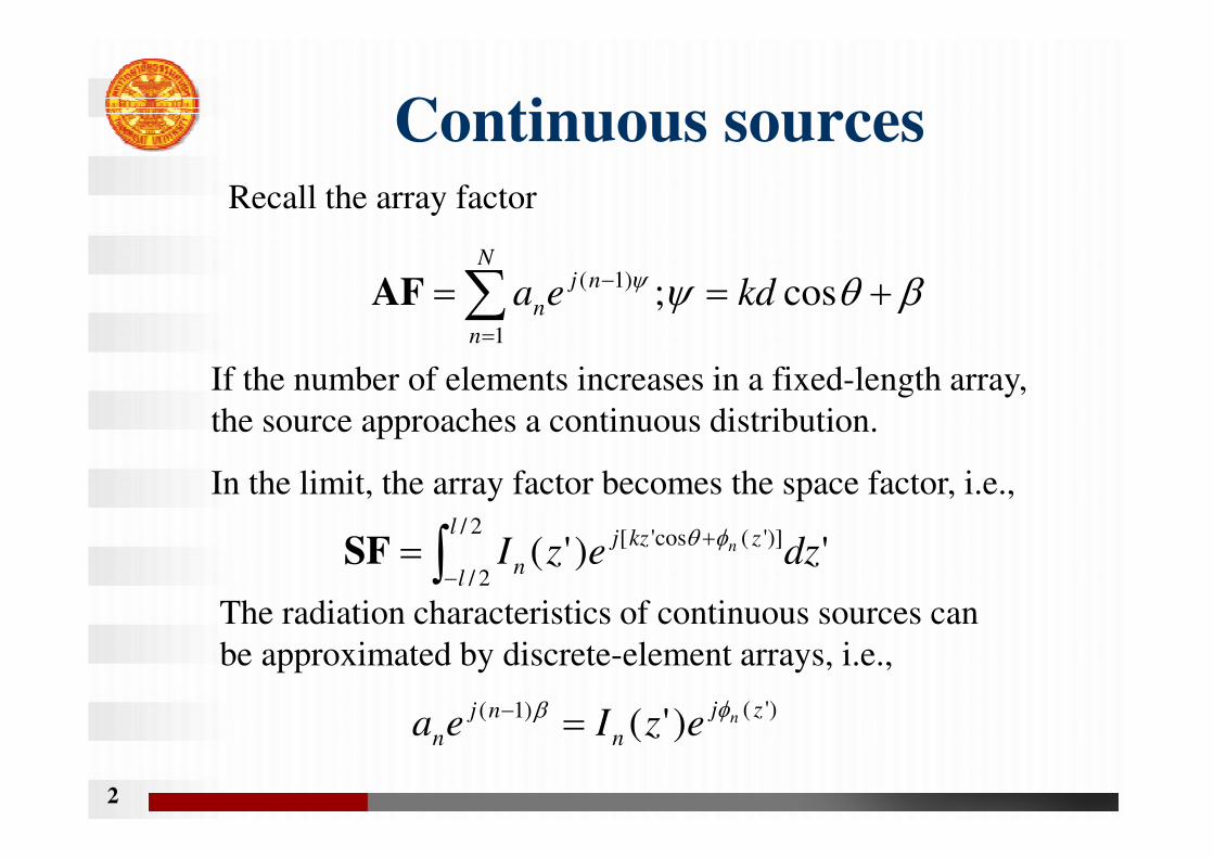
Continuous sourcesRecall the array factor
If the number of elements increases in a fixed-length array,
the source approaches a continuous distribution.
In the limit, the array factor becomes the space factor, i.e.,
N
n
nj
n kdea1
)1( cos; AF
)'()1( )'(zj
n
nj
nnezIea
The radiation characteristics of continuous sources can
be approximated by discrete-element arrays, i.e.,
2/
2/
)]'(cos'[')'(
l
l
zkzj
n dzezI nSF

3
Schelkunoff polynomial
method
)cos( kdjjeejyxz
The array factor for an N-element, equally spaced, non-
uniform amplitude, and progressive phase excitation is given
by
Let
N
n
nj
n kdea1
)1( cos; AF
N
n
N
N
n
n zazaaza1
1
21
1LAF
which is a polynomial of degree (N-1).

4
Schelkunoff polynomial
method (2)
1|||| zezzj
Thus
Note that
)())(( 121 NN zzzzzza LAF
cos2
cos dkd
z is on a unit circle.
where z1,z2,…,zN-1 are the roots. The magnitude then
becomes
|||||||||| 121 NN zzzzzza LAF
Schelkunoff polynomial
method (3)
5
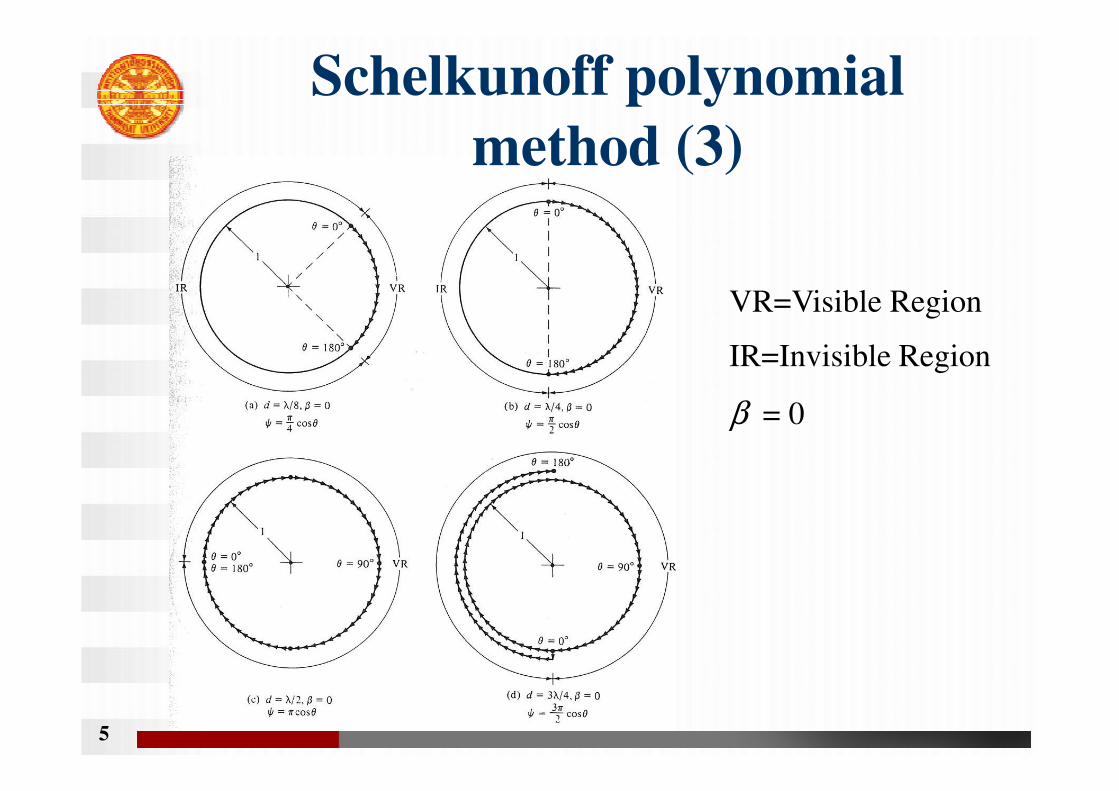
VR=Visible Region
IR=Invisible Region
β = 0

Schelkunoff polynomial
method (4)
6
VR=Visible Region
IR=Invisible Region
β = π/4

Schelkunoff polynomial
method (5)
7

Schelkunoff polynomial
method : Example
8
Design a linear array with a spacing between the elements
of d=λ/4 such that it has zeros at θ=0,π/2,π. Determine the
number of elements, their excitation, and plot the derived
pattern.

Schelkunoff polynomial
method : Example pattern
9
0 20 40 60 80 100 120 140 160 180−50
−45
−40
−35
−30
−25
−20
−15
−10
−5
0
θ [Degree]
|(A
F) n
| [d
B]
4−element array factor

Fourier Transform Method
10
The normalized space factor for a continuous line-source
distribution of length l can be given by
k
kkk
dzezIdzezI
zz
l
l
zjl
l
zkkj z
1
2/
2/
'2/
2/
)')cos(
coscos
')'(')'()(SF
where kz is the excitation phase constant of the source. If
I(z’)=I0/l,
k
kkl
k
kkl
Iz
z
cos2
cos2
sin
)( 0SF

Fourier Transform Method (2)
11
Since the current distribution extends only over -l/2≤z’≤ l/2,
')'()()( '
dzezIzj SFSF
The approximate source distribution Ia (z’) is given by
dedezI
zjzj '' )(2
1)(
2
1)'( SFSF
The current distribution can then be given by
elsewhere0
2/'2/)(2
1)'(
)'(
'lzldezI
zI
zj
a
SF
2/
2/
' ')'()()(l
l
zj
aaa dzezI SFSFThus
Fourier Transform Method : Example 7.2
12
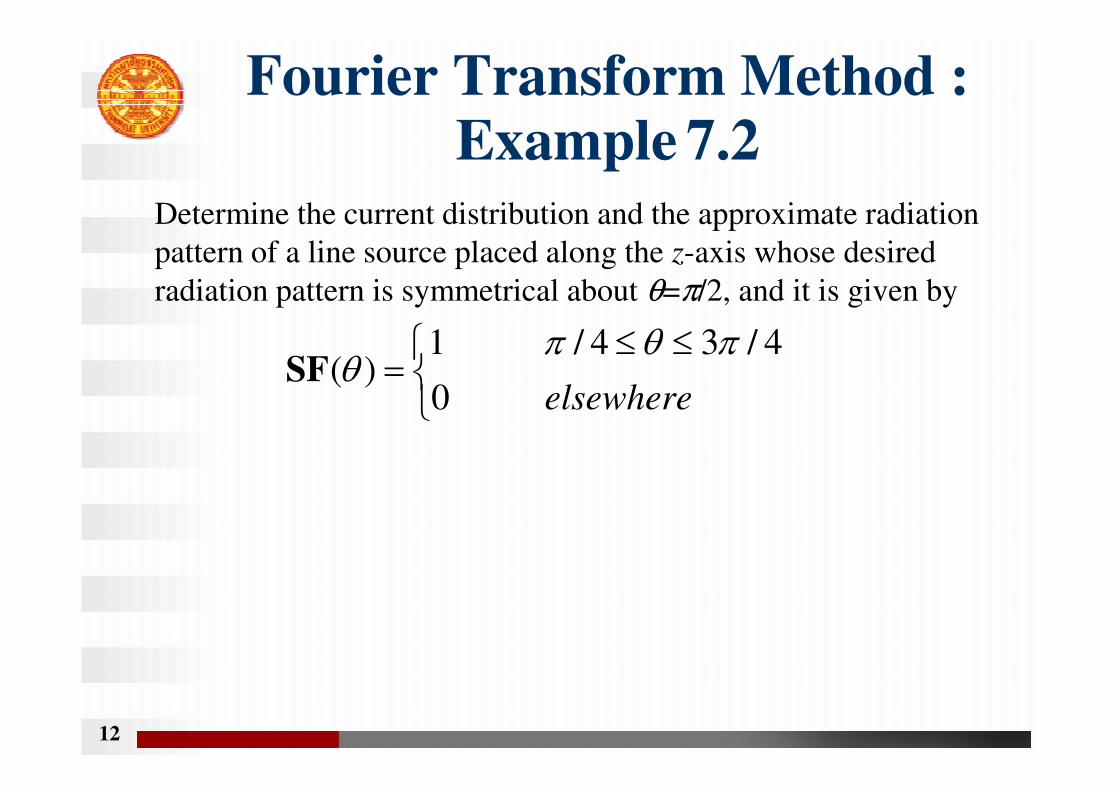
Determine the current distribution and the approximate radiation
pattern of a line source placed along the z-axis whose desired
radiation pattern is symmetrical about θ=π/2, and it is given by
elsewhere0
4/34/1)(
SF
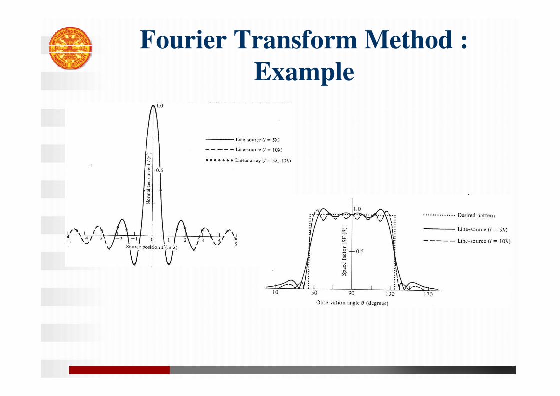
Fourier Transform Method :
Example
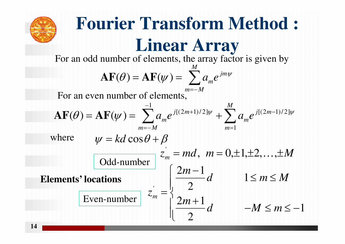
Fourier Transform Method :
Linear Array
14
For an odd number of elements, the array factor is given by
M
Mm
jm
mea )()( AFAF
where
For an even number of elements,
1
2
12
12
12
'
mMdm
Mmdm
zm
Mmmdzm ,,2,1,0,'K
Elements’ locations
M
m
mj
m
Mm
mj
m eaea1
]2/)12[(1
]2/)12[()()( AFAF
coskd
Even-number
Odd-number

Fourier Transform Method :
Linear Array (2)
15
For an odd number of elements, the excitation coefficients can
be obtained by
MmM
dedeT
ajmjm
T
Tm
)(2
1)(
1 2/
2/AFAF
where
For an even number of elements,
coskd
Mmde
mMde
amj
mj
m
1)(2
1
1)(2
1
]2/)12[(
]2/)12[(
AF
AF

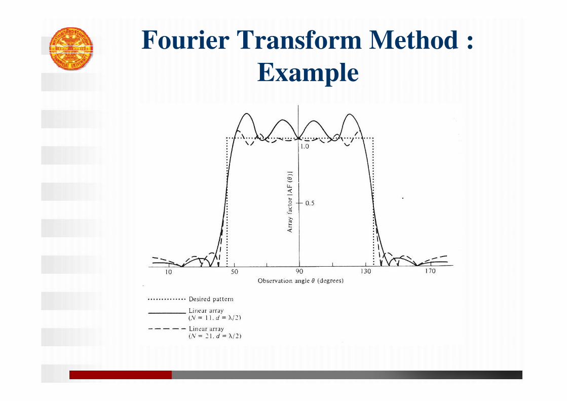
Fourier Transform Method :
Example
16
Same as Example 7.2 with d = λ/2; non-zero only
2/cos2/ kd
4/34/
thus
therefore
2
2sin
2
1
2
1 2/
2/
m
m
deajm
m
0101.00588.0
010.00518.02170.0
0455.00895.03582.0
0496.00578.00.1
73
1062
951
840
aa
aaa
aaa
aaa
Result
Fourier Transform Method :
Example

Quiz
A 5-element uniform linear array with a
spacing of λλλλ between elements is designed
to scan at θθθθ=ππππ/3. Assume that the array is
aligned along the z-axis.
a) Find the array factor
b) Find the angle of the grating lobe.
c) Find the condition such that there exists no
grating lobe.

Quiz solution
0 20 40 60 80 100 120 140 160 1800
0.1
0.2
0.3
0.4
0.5
0.6
0.7
0.8
0.9
1
θ [Degree]
|(A
F) n
| [d
B]
5−element array factor
d=λ
d=5λ/8
d=λ/2
Woodward-Lawson Method• Sampling the desired pattern at various discrete
locations.
• Use composing function of the forms:
as the field of each pattern sample
• The synthesized pattern is represented by a finite
sum of composing functions.
• The total excitation is a sum of space harmonics.
mmmmmm NNbb sin/)sin(or /)sin(
Woodward-Lawson Method:
Line-source
2/'2/)'(cos'
lzlel
bzi mjkzm
m
M
Mm
jkz
mmeb
lzI
cos'1)'(
number) odd 12(for ,,2,1,0
number)even 2(for ,,2,1 where
MMm
MMm
K
K
m
m
mm kl
kl
bs
coscos2
coscos2
sin
)(
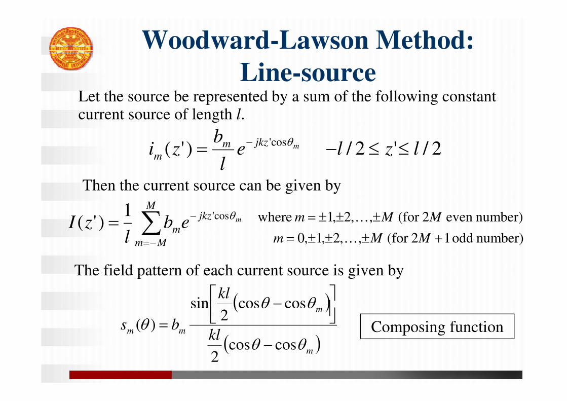
Let the source be represented by a sum of the following constant current source of length l.
Then the current source can be given by
The field pattern of each current source is given by
Composing function

Woodward-Lawson Method:
Line-source (2)
dmmb )(SF
lkz lz
2' '||
For an odd number samples, the total pattern becomes
bm can be obtained from the value at the sample points θm, i.e.,
In order to satisfy the periodicity of 2π and faithfully reconstruct the desired pattern,
M
Mmm
m
m kl
kl
b
coscos2
coscos2
sin
)(SF

Woodward-Lawson Method:
Line-source (3)
samples oddfor ,2,1,0,cos K
ml
mmm
Thus the location of each sample is given by
Therefore, M should be the closest integer to M=l/λ.
sampleseven for
,2,1,2
12
2
12
,2,1,2
12
2
12
cos
K
K
ml
mm
ml
mm
m

Woodward-Lawson Method:
Example
5,,2,1,0),2.0(cos)(cos 11 Kmmmm
Same as Example 7.2; for l = 5λ.Since l = 5λ, M = 5 and ∆ = 0.2.
m θθθθm bmm θθθθm bm
0 90 1
1 78.46 1 -1 101.54 1
2 66.42 1 -2 113.58 1
3 53.13 1 -3 126.87 1
4 36.87 0 -4 143.13 0
5 0 0 -5 180 0
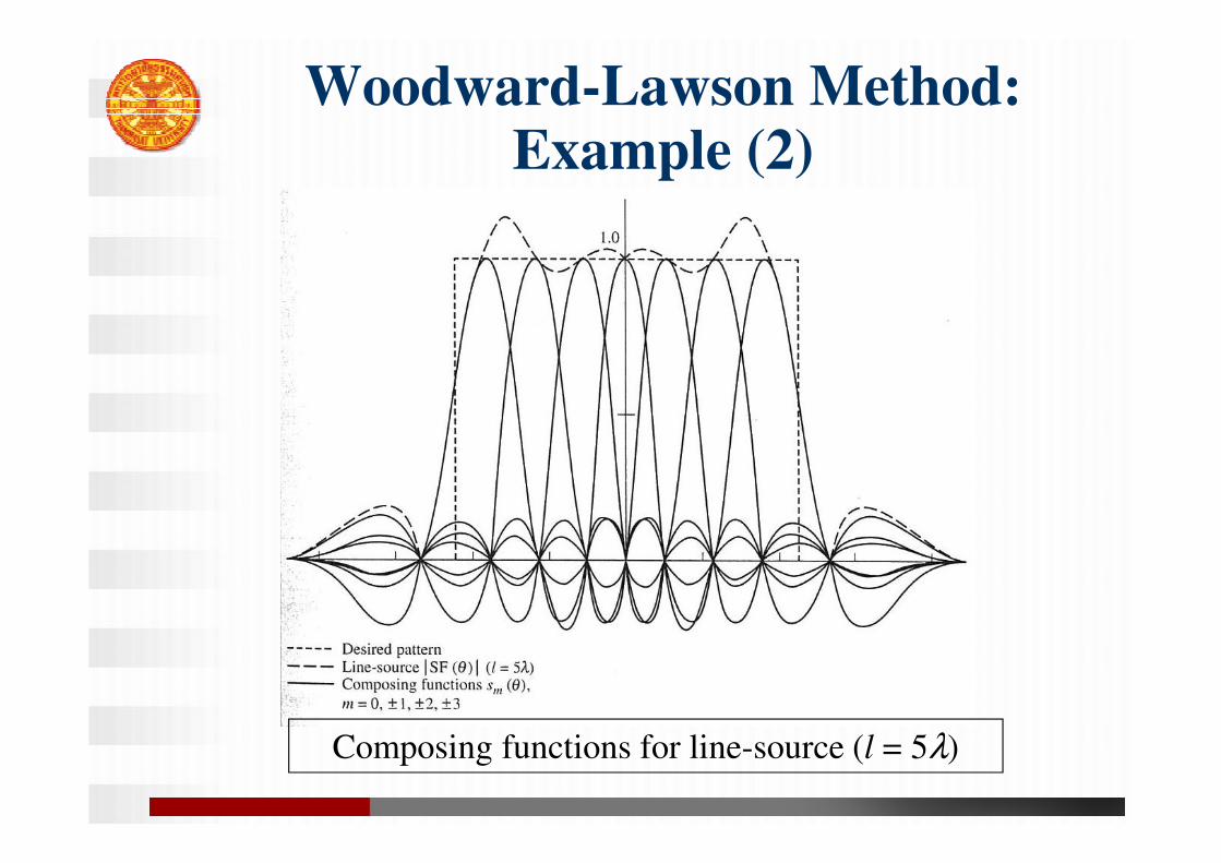
Woodward-Lawson Method: Example (2)
Composing functions for line-source (l = 5λ)
Woodward-Lawson Method:
Linear array
m
m
mm kdN
kdN
bf
coscos2
sin
coscos2
sin
)(
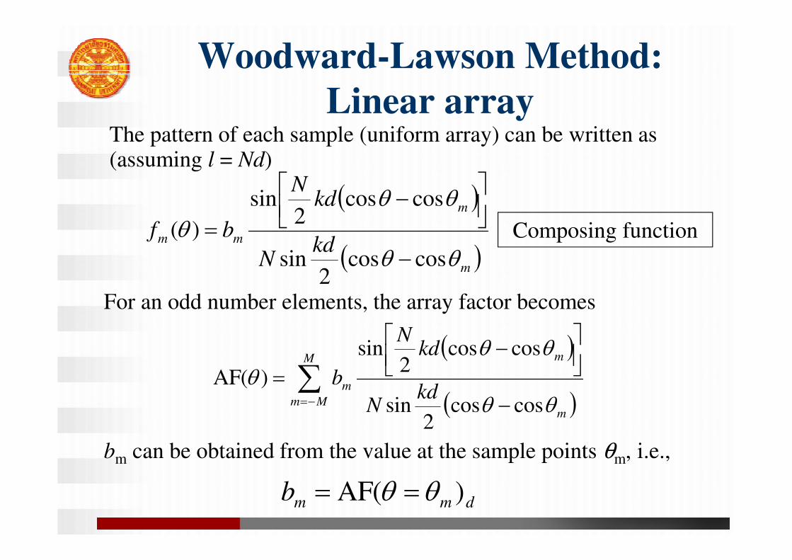
The pattern of each sample (uniform array) can be written as (assuming l = Nd)
Composing function
M
Mmm
m
m kdN
kdN
b
coscos2
sin
coscos2
sin
)(AF
dmmb )(AF
For an odd number elements, the array factor becomes
bm can be obtained from the value at the sample points θm, i.e.,
Woodward-Lawson Method:
Linear array (2)
sampleseven for
,2,1,2
12
2
12
,2,1,2
12
2
12
cos
K
K
mNd
mm
mNd
mm
m
samples oddfor ,2,1,0,cos K
mNd
mmm
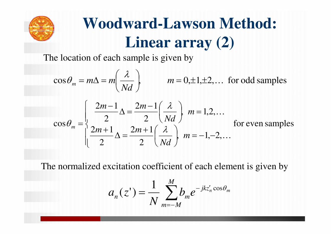
The location of each sample is given by
The normalized excitation coefficient of each element is given by
M
Mm
zjk
mnmneb
Nza
cos1)'(

Woodward-Lawson Method:
Example
Element number
n
Position
z’n
Coefficient
an
±1 ±0.25λλλλ 0.5696
±2 ± 0.75λλλλ -0.0345
±3 ± 1.25λλλλ -0.1001
±4 ± 1.75λλλλ 0.1108
±5 ± 2.25λλλλ -0.0460
Same as Example 7.2; for N=10 and d = λ/2.
The coefficients can be found to be
To obtain the normalized amplitude pattern of unity at θ=π/2,
the array factor has been divided by 4998.0na

Woodward-Lawson Method:
Example
0 20 40 60 80 100 120 140 160 1800
0.2
0.4
0.6
0.8
1
1.2
1.4
θ [Degree]
No
rma
lize
d m
ag
nitu
de
Line−source
Linear Array (N=10,d=λ/2)
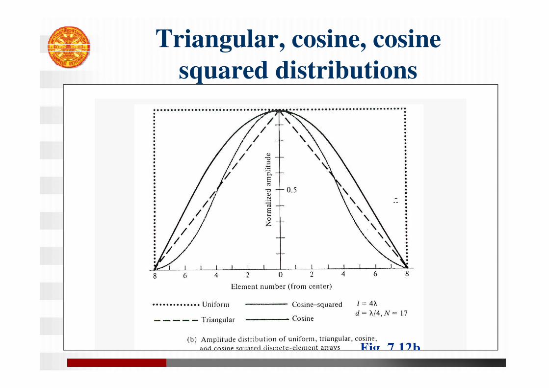
Triangular, cosine, cosine
squared distributions

32
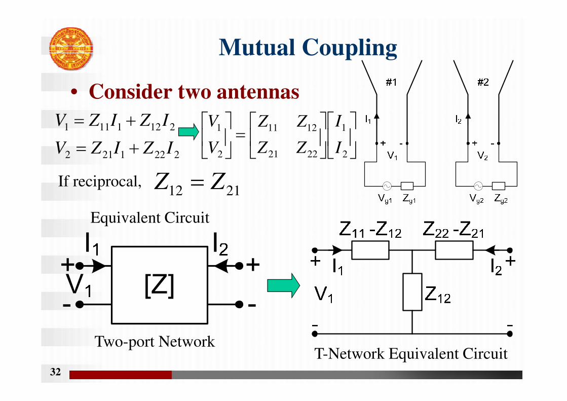
Mutual Coupling
• Consider two antennas
2221212
2121111
IZIZV
IZIZV
2
1
2221
1211
2
1
I
I
ZZ
ZZ
V
V
2112 ZZ If reciprocal,
Equivalent Circuit
Two-port NetworkT-Network Equivalent Circuit

Mutual Coupling: 2 antennas
01
111
2
I
I
VZ
02
112
1
I
I
VZ
01
221
2
I
I
VZ
02
222
1
I
I
VZ
impedancepoint driving
active
21
ddZ
1
21211
1
11
I
IZZ
I
VZ d
2112 ZZ
for reciprocal networks
:, 2211 ZZ
Input impedance
2
12122
2
22
I
IZZ
I
VZ d
2
12
1
21 on depends ;on depends :Note
I
IZ
I
IZ dd

Mutual Coupling: 2 antennas (2)
• As I1 and I2 change, the driving point impedance changes.
• In a uniform array, the phase of I1 and I2
is changed to scan the beam.
• As the beam is scanned, the driving port impedance in each antenna changes.
• In general, Z11,Z12=Z21,Z22 can be calculated using numerical techniques.
• For some special cases, they can be calculated analytically.
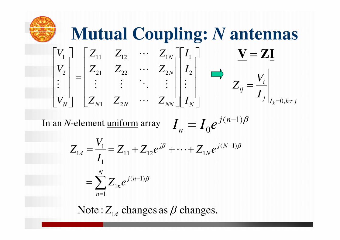
Mutual Coupling: N antennas
NNNNN
N
N
N I
I
I
ZZZ
ZZZ
ZZZ
V
V
V
M
L
MOMM
L
L
M
2
1
21
22221
11211
2
1 IZV
jkIj
iij
k
I
VZ
,0
In an N-element uniform array )1(
0
nj
n eII
N
n
nj
n
Nj
N
j
d
eZ
eZeZZI
VZ
1
)1(
1
)1(
11211
1
11
L
changes. as changes :Note 1 dZ
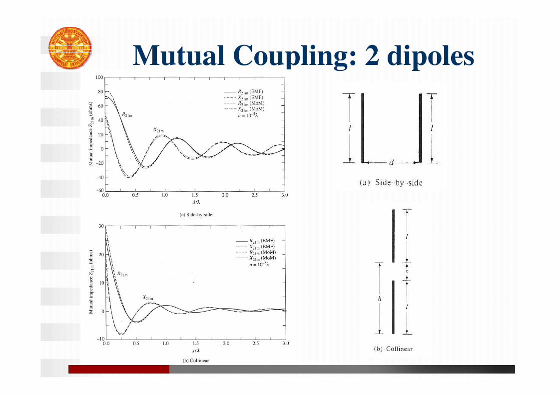
Mutual Coupling: 2 dipoles
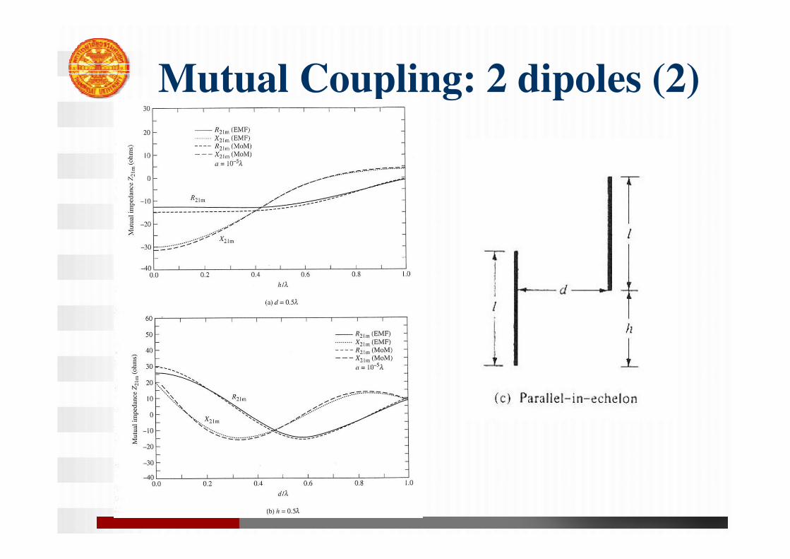
Mutual Coupling: 2 dipoles (2)


![Patch Antenna[1]](https://static.fdokumen.com/doc/165x107/63158e4cc32ab5e46f0d5c89/patch-antenna1.jpg)