Fog Forecast Using WRF Model Output for Solar ... - MDPI

energies

Article

Fog Forecast Using WRF Model Output for SolarEnergy Applications

Saverio Teodosio Nilo 1,* , Domenico Cimini 1,2 , Francesco Di Paola 1 ,Donatello Gallucci 1 , Sabrina Gentile 1,2 , Edoardo Geraldi 1 , Salvatore Larosa 1 ,Elisabetta Ricciardelli 1, Ermann Ripepi 1 , Mariassunta Viggiano 1 and Filomena Romano 1

1 Institute of Methodologies for Environmental Analysis, National Research Council (IMAA-CNR),85100 Potenza, Italy; [email protected] (D.C.); [email protected] (F.D.P.);[email protected] (D.G.); [email protected] (S.G.); [email protected] (E.G.);[email protected] (S.L.); [email protected] (E.R.); [email protected] (E.R.);[email protected] (M.V.); [email protected] (F.R.)

2 Center of Excellence Telesensing of Environment and Model Prediction of Severe Events (CETEMPS),University of L’Aquila, 67100 L’Aquila, Italy

* Correspondence: [email protected]; Tel.: +39-0971-427295

Received: 28 October 2020; Accepted: 20 November 2020; Published: 23 November 2020 ��

Abstract: The occurrence of fog often causes errors in the prediction of the incident solar radiationand the power produced by photovoltaic cells. An accurate fog forecast would benefit solar energyproducers and grid operators, who could take coordinated actions to reduce the impact of discontinuity,the main drawback of renewable energy sources. Considering that information on discontinuity iscrucial to optimize power production estimation and plant management efficiency, in this work, a fogforecast method based on the output of the Weather Research and Forecasting (WRF) numerical modelis presented. The areal extension and temporal duration of a fog event are not easy to predict. In fact,there are many physical processes and boundary conditions that cause fog development, such as thesynoptic situation, air stability, wind speed, season, aerosol load, orographic influence, humidity andtemperature. These make fog formation a complex and rather localized event. Thus, the results of afog forecast method based on the output variables of the high spatial resolution WRF model stronglydepend on the specific site under investigation. In this work, the thresholds are site-specificallydesigned so that the implemented method can be generalized to other sites after a preliminarymeteorological and climatological study. The proposed method is able to predict fog in the 6–30 hinterval after the model run start time; it has been evaluated against METeorological AerodromeReport data relative to seven selected sites, obtaining an average accuracy of 0.96, probability ofdetection of 0.83, probability of false detection equal to 0.03 and probability of false alarm of 0.18.The output of the proposed fog forecast method can activate (or not) a specific fog postprocessinglayer designed to correct the global horizontal irradiance forecasted by the WRF model in order tooptimize the forecast of the irradiance reaching the photovoltaic panels surface.

Keywords: fog forecast; numerical weather prediction; WRF; solar energy; power production forecast

1. Introduction

Fog is defined as consisting of tiny droplets of water or ice crystals with a diameter between~5–30 µm suspended in the immediate vicinity of the Earth’s surface, able to decrease the horizontalvisibility down to less than 1 km [1]. Fog is a microscale phenomenon as it is directly influenced bylocal surface forcing and weather conditions, with a time scale of hours or less [2]. Fog has severalimplications on the atmosphere and the environment, leading to numerous direct and indirect effects

Energies 2020, 13, 6140; doi:10.3390/en13226140 www.mdpi.com/journal/energies

http://www.mdpi.com/journal/energies

http://www.mdpi.com

https://orcid.org/0000-0003-2630-8727

https://orcid.org/0000-0002-5962-223X

https://orcid.org/0000-0001-9892-0582

https://orcid.org/0000-0002-6814-193X

https://orcid.org/0000-0002-3892-970X

https://orcid.org/0000-0003-3949-512X

https://orcid.org/0000-0003-2588-6082

https://orcid.org/0000-0002-6304-4655

https://orcid.org/0000-0003-2462-3619

https://orcid.org/0000-0002-0544-073X

http://dx.doi.org/10.3390/en13226140

http://www.mdpi.com/journal/energies

https://www.mdpi.com/1996-1073/13/22/6140?type=check_update&version=2

Energies 2020, 13, 6140 2 of 28

on life and human activities, particularly in meteorology, climatology, transports, energy, agriculture,economy and ecology [3–6]. The main consequence of fog is visibility reduction that can lead tofinancial damages, severe accidents and loss of lives [7–9]. Thus, fog prediction has always beenan extremely important activity for land, sea and air transport sectors [10]. Moreover, the presenceof fog tends to alter the radiative budget of the Earth–atmosphere system, hence it is important inmeteorology because it can perturb the local temperature and humidity [11]. It impacts air qualitybecause it develops when thermal inversions persist; in this situation, air pollutants are trapped in theboundary layer and not scattered in the atmosphere, especially in urban and industrialized areas [12].Fog also scatters solar radiation, decreasing the power produced by photovoltaic panels. Fog scattering,in fact, reduces to zero the direct component of incoming solar radiation, which represents the maincontribution to the electric power produced by photovoltaic panels [13,14]. Thus, fog forecast isuseful to correct solar irradiance prediction and, accordingly, the power produced by solar systems.This certainly represents one of the frontiers of meteorology applied to renewable energy. In this sense,the fog forecast assumes a value that economically impacts the supply of solar energy on the marketbecause the evaluation of the goodness of the forecast is related to an economic index, i.e., the lowestpossible imbalance between the expected energy offered on the trading market and the measuredfinal balance. Early attempts in forecasting fog are found in [15], where a method for predicting fogduring night based on observations at 8:00 p.m. was presented. Cooling of moist air by radiative fluxdivergence, vertical mixing of heat and moisture, vegetation, horizontal and vertical wind, heat andmoisture transport in soil, advection and topographic effect are all listed in [16] as important processesto consider in the fog formation, whilst longwave radiative cooling at fog top, gravitational dropletsettling, fog microphysics and shortwave radiation are important processes driving fog duration.

In general, there are two broad categories of fog forecast: numerical (using computer simulations)and observational (diagnosing the likelihood of a future event based on current observations).An approach to implement fog forecast is to use statistics to define threshold values for key variablesinvolved in the fog formation and to verify its predictability using observations and NWP modeloutputs. Among the statistical methods, different data mining, machine learning and multivariatetechniques have been developed [17–19]. In [20], the proposed statistical method assigns a likelihood offog occurrence from 0 to 1 based on comparing observations of key variables to predefined thresholds.

Another methodology is based on NWP fog simulation in terms of liquid water content or otherthermodynamic quantities and processes (horizontal pressure gradient, advection, diffusion, etc.).These models are able to simulate radiation fog when configured with sophisticated options andhigh horizontal and vertical resolutions and can be implemented for fog forecast in one dimension(1D) similarly to other works [19,21–27]. The main limitation of these 1D methods is their poorrepresentation of the large-scale situation. Thus, three-dimensional (3D) mesoscale models such as theFifth-Generation NCAR/Penn State Mesoscale Model (MM5) and the Weather Research and Forecasting(WRF) model are also used [8,19,28–31]. Fog forecast with NWP models is still a challenge, with limitedsuccess in terms of accuracy and precision. This is mainly due to the intrinsically complex nature ofthe fog phenomenon and to the limited availability of observational and computational resources.

Some empirical methods, instead, are mainly based on thermal and hygrometric gradients betweensoil and medium-low troposphere [32–38]. However, these indices need to be adapted on the basis ofthe historical series and the local conditions, in order to include small scale factors like local advectivetransport, radiation, turbulent mixing, orography and to produce a multiapproach scheme for fogforecast [34,39].

The implementation of a new fog forecast method represents the main objective of this work.Fog forecast is a rather complex task because of the extreme variability of the conditions that lead toits development, the relatively low knowledge about atmospheric phenomena and the coexistenceand interaction of processes characterized by different time and spatial scales. Furthermore, fog isa local forced event that can rapidly grow or dissipate in conditions not uniquely defined. This isthe main aspect we focus on in this research: the characterization of site-specific meteorological

Energies 2020, 13, 6140 3 of 28

conditions that promote fog formation. The method to predict fog has been implemented usingthe output of a numerical weather prediction model. The selected domain is the Italian peninsula.In this territory, the Po Valley, the Apennines and Alpine valleys are often affected by fog duringautumn and winter, especially in the morning hours, when a high-pressure stable condition andthermal inversion near the ground are present [2,40]. This kind of fog event has the highest impacton photovoltaic power production [13]. Solar energy is produced by converting the incoming solarradiation reaching the photovoltaic panel surfaces. Solar radiation enters the atmosphere and undergoesphysical and photochemical interactions which determine a partial or total extinction. In particular,the atmospheric attenuation is due to the combined effects of backscattering and absorption by cloudsand aerosol, the backscattering due to the air molecules and the absorption by the gases according tothe Bouguer–Lambert–Beer law [14]. In absorption, a fraction of the energy that propagates through alayer of air is absorbed by the atmospheric constituents and can be re-emitted at a different wavelength.In addition to absorption, a fraction of the radiant energy that passes through the atmosphere isscattered. The scattering is mainly due to the impact with air molecules, dust and liquid water dropletswhich causes a portion of radiation to be reflected back in all directions (back scattering) or sent tothe Earth in a diffuse form (forward scattering) [9]. Among the different types of clouds, we areinterested in the specific effects of fog on the solar irradiance and, consequently, on photovoltaic powerproduction. Fog affects solar radiation through Mie scattering and redistributing incident radiationin different directions according to the particle size. This means that in the fog condition, the diffusecomponent can account almost for all the incoming solar radiation. Hence, fog dramatically impactsthe solar power production forecast when clear sky conditions are expected but a fog event occurs [13].This happens especially in the first hours of daylight until solar heating triggers the fog dissolutionprocess. The WRF model running at IMAA-CNR forecasts the global horizontal irradiance (GHI)and its direct and diffuse components. In particular, given the wide availability of measurements,we decided to focus on the GHI. Our idea is to adjust the WRF GHI output in those cases where theWRF model did not foresee fog while our multitest-based method for fog forecasting (MBFog) didit by activating a fog postprocessing layer. The fog postprocessing layer is designed to apply a fogattenuation transmittance coefficient to the GHI WRF outputs in order to optimize the forecast of theirradiance reaching the Earth’s surface. This transmittance is obtained using a parameterization ofthe fog extinction coefficient [41] and is a function of the solar elevation angle. In Section 2, the useddataset and the implemented methodology are introduced. Section 3 reports the main results and theirdiscussion, while Section 4 reports the conclusions of the study.

2. Materials and Methods

First, we introduce the METeorological Aerodrome Report, the surface SYNOPtic observations andthe European Centre for Medium-Range Weather Forecasts reanalysis dataset. Successively, the specificconfiguration of the WRF NWP model used for the development of the fog forecast methodologyis described.

2.1. METAR and SYNOP Dataset

METeorological Aerodrome Reports (METAR) data are collected in aeronautical weather stations.Data collection can be regular or special. Regular measurements are done at fixed temporal rate(10, 20, 30 or 60 min) while special measurements are taken when a significant variation of the weatherbetween two regular reports occurs. For the fog presence verification purpose, we focus on the visibilityMETAR data. The Italian METAR network features both fully and partially automated stations [42].This means that some METAR stations are supervised by an observer who manually reports therelevant information when necessary. Although the METAR can contain the specification about thedirection in which the visibility measurements have been acquired, in our study, we considered only360◦ visibility data, with no indication on direction. Since vertical visibility is not always available,it was not considered in this study. Daylight hourly METAR reports are used as the source of

Energies 2020, 13, 6140 4 of 28

predictand—i.e., the presence of fog. Fog is detected based on two conditions: (i) reported hourlyvisibility is less than 1 km (according to WMO fog definition) and (ii) the label “FG” alone (indicating fogcondition) is reported in the METAR present weather field. In this way, the reduction of visibility hasbeen attributed uniquely to the presence of fog and not to other weather conditions such as intenserain, thunderstorm, sand, or ash.

Moreover, METAR wind speeds recorded during the period 2011–2017 (in case fog condition wasreported) were used in this study to define thresholds. METAR visibility data were used twofold:(i) for the climatological featuring of the main meteorological variables involved in the fog forecastingalgorithm, and (ii) for the evaluation of the implemented method. To evaluate the proposed method,an independent METAR dataset was collected, covering a different time interval (January to April 2018)and relative to seven sites in Italy selected based on fog occurrences.

SYNOP bulletins are produced based on the same METAR measurements, but at higher signalresolution. SYNOP values of surface and dew point temperature, recorded with one tenth of degreeresolution, were collected for the period 2011–2017 (in the case fog condition was reported) and used inthis work to define thresholds. The SYNOP bulletins are issued worldwide at least on a six-hour basis;in Italy, the release frequency is three hours. We have therefore performed a temporal interpolation ofthese measurements to obtain the hourly frequency required in our study. METAR reports and SYNOPbulletins used in this work are property of the Italian Air Force Meteorological Service. Data wereprovided under the Educational/Research license.

2.2. ECMWF ERA5 HRES Reanalysis

The European Centre for Medium-Range Weather Forecasts (ECMWF) ERA5 HRES dataset [43]provides several meteorological variables at one-hour time resolution. It is a global climate reanalysisdataset with 0.25 by 0.25 degrees spatial resolution, covering the period 1950 to present. The reanalysis isa numerical description of the atmospheric conditions obtained combining models with a comprehensiveset of observations.

ERA5 HRES is produced using 4D-Var data assimilation in CY41R2 Version of the ECMWF’sIntegrated Forecast System (IFS) model, with 137 hybrid sigma/pressure vertical levels, with the toplevel at 0.01 hPa. Atmospheric data are available for these levels and they are also interpolated to37 pressure, 16 potential temperature and 1 potential vorticity level(s). Among the hundreds of ERA5HRES variables we have selected the ones closely related to fog: relative humidity, temperature anddew point at 2 m and wind speed at 10 m.

2.3. WRF Numerical Weather Prediction Model

The Solar Version [44] of the WRF numerical weather prediction model is currently operativeat the Institute of Methodologies for Environmental Analysis of the National Research Council ofItaly (IMAA-CNR). WRF is a limited area model developed by the National Center for AtmosphericResearch (NCAR). WRF-Solar Version has been released from the Version 3.6 [45] and is designed to beused in the field of solar energy, thanks to the addition of specific tools. The main features of the WRFmodel are briefly described below.

The WRF is a nonhydrostatic NWP that solves and integrates the atmospheric dynamics equations;these are formulated using the terrain following vertical coordinate eta [45]. The numerical schemeused to integrate the low frequency modes (meteorological phenomena) is the third order Runge–Kuttamethod, while the forward/backward one is used for the high-frequency modes (acoustic andgravitational waves). As far as physics is concerned, WRF contains several options for eachparameterized category, allowing them to be selected and combined according to the objectiveof the work. The parametrized physical categories are microphysics, convection, planetary boundarylayer (PBL), surface model and radiation. Microphysics explicitly resolves the precipitation, vapor andcloud processes. The convective scheme reproduces vertical flows, and it is used only on low spatialresolution domains (>3–5 km) where convective eddies cannot be explicitly resolved. The PBL schemes

Energies 2020, 13, 6140 5 of 28

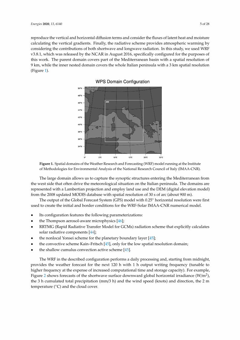
reproduce the vertical and horizontal diffusion terms and consider the fluxes of latent heat and moisturecalculating the vertical gradients. Finally, the radiative scheme provides atmospheric warming byconsidering the contributions of both shortwave and longwave radiation. In this study, we used WRFv3.8.1, which was released by the NCAR in August 2016, specifically configured for the purposes ofthis work. The parent domain covers part of the Mediterranean basin with a spatial resolution of9 km, while the inner nested domain covers the whole Italian peninsula with a 3 km spatial resolution(Figure 1).

Energies 2020, 13, x FOR PEER REVIEW 5 of 30

we used WRF v3.8.1, which was released by the NCAR in August 2016, specifically configured for the purposes of this work. The parent domain covers part of the Mediterranean basin with a spatial resolution of 9 km, while the inner nested domain covers the whole Italian peninsula with a 3 km spatial resolution (Figure 1).

Figure 1. Spatial domains of the Weather Research and Forecasting (WRF) model running at the In-stitute of Methodologies for Environmental Analysis of the National Research Council of Italy (IMAA-CNR).

The large domain allows us to capture the synoptic structures entering the Mediterranean from the west side that often drive the meteorological situation on the Italian peninsula. The domains are represented with a Lambertian projection and employ land use and the DEM (digital elevation model) from the 2008 updated MODIS database with spatial resolution of 30 s of arc (about 900 m).

The output of the Global Forecast System (GFS) model with 0.25° horizontal resolution were first used to create the initial and border conditions for the WRF-Solar IMAA-CNR numerical model.

Its configuration features the following parameterizations:

• the Thompson aerosol-aware microphysics [46]; • RRTMG (Rapid Radiative Transfer Model for GCMs) radiation scheme that explicitly calculates

solar radiative components [44]; • the nonlocal Yonsei scheme for the planetary boundary layer [45]; • the convective scheme Kain–Fritsch [45], only for the low spatial resolution domain; • the shallow cumulus convection active scheme [45].

The WRF in the described configuration performs a daily processing and, starting from mid-night, provides the weather forecast for the next 120 h with 1 h output writing frequency (tunable to higher frequency at the expense of increased computational time and storage capacity). For example, Figure 2 shows forecasts of the shortwave surface downward global horizontal irradiance (W/m2), the 3 h cumulated total precipitation (mm/3 h) and the wind speed (knots) and direction, the 2 m temperature (°C) and the cloud cover.

Figure 1. Spatial domains of the Weather Research and Forecasting (WRF) model running at the Instituteof Methodologies for Environmental Analysis of the National Research Council of Italy (IMAA-CNR).

The large domain allows us to capture the synoptic structures entering the Mediterranean fromthe west side that often drive the meteorological situation on the Italian peninsula. The domains arerepresented with a Lambertian projection and employ land use and the DEM (digital elevation model)from the 2008 updated MODIS database with spatial resolution of 30 s of arc (about 900 m).

The output of the Global Forecast System (GFS) model with 0.25◦ horizontal resolution were firstused to create the initial and border conditions for the WRF-Solar IMAA-CNR numerical model.

• Its configuration features the following parameterizations:• the Thompson aerosol-aware microphysics [46];• RRTMG (Rapid Radiative Transfer Model for GCMs) radiation scheme that explicitly calculates

solar radiative components [44];• the nonlocal Yonsei scheme for the planetary boundary layer [45];• the convective scheme Kain–Fritsch [45], only for the low spatial resolution domain;• the shallow cumulus convection active scheme [45].

The WRF in the described configuration performs a daily processing and, starting from midnight,provides the weather forecast for the next 120 h with 1 h output writing frequency (tunable tohigher frequency at the expense of increased computational time and storage capacity). For example,Figure 2 shows forecasts of the shortwave surface downward global horizontal irradiance (W/m2),the 3 h cumulated total precipitation (mm/3 h) and the wind speed (knots) and direction, the 2 mtemperature (◦C) and the cloud cover.

Energies 2020, 13, 6140 6 of 28Energies 2020, 13, x FOR PEER REVIEW 6 of 30

(a) (b)

(c) (d)

Figure 2. Example of IMAA-CNR WRF products. Run of 04/09/18 at 00:00 UTC, forecast valid at 14:00 UTC on 04 September 18. Variables forecasted: (a) global horizontal irradiance (W/m2), (b) 3 h cumu-lated total precipitation (mm/3 h) plus wind speed (knots) and direction, (c) surface temperature (°C), (d) cloud cover.

2.4. The MBFog Multitest Approach

In this study, a multitest-based method for fog forecasting (MBFog) is proposed. It was preferred to the single diagnostic approach because of limits that the latter shows in fog prediction [9,33]. Mul-titest-based approaches use two or more variables depending on the desired fog characterization. In particular, in [33], three tests were used to deal with different fog types: liquid water content (LWC), cloud base/top and surface relative humidity (RH)—wind rules. Since LWC is related to the horizon-tal visibility according to Kunkel equation [41], the LWC rule assumes fog condition, i.e., visibility of 1 km or less, when LWC is larger than 0.015 g/kg. Cloud base/top rule uses the nominal vertical features of fog (base of 50 m or less, top of 400 m or less) to identify a fog event. Finally, RH-wind rule identifies fog when two meteorological situations occur: a 2 m relative humidity of 90% or more and a 10 m wind speed of 2 m/s or less. In [39], the authors demonstrated that cloud base/top rule is good for a large-scale fog event like marine fog or coastal fog; for this reason, the RH-wind rule and a two-level approach using the temperature gradient rule were considered, in order to forecast shal-low ground fog. The proposed method is a diagnostic forecast methodology based on the combina-tion of different threshold tests applied to WRF model variables outputs, as shown in Figure 3. The main variables involved in the fog process, such as temperature, humidity, wind and dew point, are considered for threshold tests. The MBFog method is a combination of the tests implemented in [34,39] with the fog stability index [38,47] test. The fog stability index (FSI) is obtained according to the following formula:

Figure 2. Example of IMAA-CNR WRF products. Run of 04/09/18 at 00:00 UTC, forecast valid at 14:00UTC on 04 September 18. Variables forecasted: (a) global horizontal irradiance (W/m2), (b) 3 h cumulatedtotal precipitation (mm/3 h) plus wind speed (knots) and direction, (c) surface temperature (◦C),(d) cloud cover.

2.4. The MBFog Multitest Approach

In this study, a multitest-based method for fog forecasting (MBFog) is proposed. It was preferredto the single diagnostic approach because of limits that the latter shows in fog prediction [9,33].Multitest-based approaches use two or more variables depending on the desired fog characterization.In particular, in [33], three tests were used to deal with different fog types: liquid water content (LWC),cloud base/top and surface relative humidity (RH)—wind rules. Since LWC is related to the horizontalvisibility according to Kunkel equation [41], the LWC rule assumes fog condition, i.e., visibility of 1 kmor less, when LWC is larger than 0.015 g/kg. Cloud base/top rule uses the nominal vertical features offog (base of 50 m or less, top of 400 m or less) to identify a fog event. Finally, RH-wind rule identifiesfog when two meteorological situations occur: a 2 m relative humidity of 90% or more and a 10 mwind speed of 2 m/s or less. In [39], the authors demonstrated that cloud base/top rule is good for alarge-scale fog event like marine fog or coastal fog; for this reason, the RH-wind rule and a two-levelapproach using the temperature gradient rule were considered, in order to forecast shallow groundfog. The proposed method is a diagnostic forecast methodology based on the combination of differentthreshold tests applied to WRF model variables outputs, as shown in Figure 3. The main variablesinvolved in the fog process, such as temperature, humidity, wind and dew point, are considered for

Energies 2020, 13, 6140 7 of 28

threshold tests. The MBFog method is a combination of the tests implemented in [34,39] with the fogstability index [38,47] test. The fog stability index (FSI) is obtained according to the following formula:

FSI = 2(Ts − Td) + 2(Ts − T850) + WS850 (1)

where:

• Ts is the surface temperature [K],• Td is the surface dew point temperature [K],• T850 is the temperature at 850 hPa [K],• WS850 is the wind at 850 hPa [m/s].


= 2 − + 2 − + (1)

where:

• is the surface temperature [K], • is the surface dew point temperature [K], • is the temperature at 850 hPa [K], • and • is the wind at 850 hPa [m/s].

Figure 3. Block diagram of the multitest-based method for forecasting fog (MBFog) using WRF out-put. Thresholds are fixed after site-specific climatological study (test #2, #3, #4), statistical study (test #1) or literature review (test #5).

The first term, − , is the dew point depression and provides information regarding the avail-ability of moisture content in the surface proximity. The second term, − , is the stability term and gives an estimation of the atmosphere steadiness. The FSI index can assume continue values between 0 and 100, an appropriate threshold identifies FSI values related to fog condition.

To summarize, the MBFog approach presented here considers the following criteria to derive the fog forecast:

• test #1—FSI_test: fog stability index under a threshold (FSI_thresh); • test #2—RH_test: surface relative humidity over a threshold (RH_thresh); • test #3—Tdepr_test: difference between surface temperature and surface dew point under a

threshold (Tdepr_thresh); • test #4—WS_test: wind speed at 10 m between two thresholds (WS_min_thresh and

WS_max_thresh); • test #5—RHDiff_test: relative humidity difference between the first two vertical levels under a

threshold (RHDiff_thresh).

The last rule tends to identify the cases featuring negative relative humidity gradient between two layers next to the surface as “no fog”. The main meteorological variables involved in fog onset

Figure 3. Block diagram of the multitest-based method for forecasting fog (MBFog) using WRF output.Thresholds are fixed after site-specific climatological study (test #2, #3, #4), statistical study (test #1) orliterature review (test #5).

The first term, Ts − Td, is the dew point depression and provides information regarding theavailability of moisture content in the surface proximity. The second term, Ts − T850, is the stabilityterm and gives an estimation of the atmosphere steadiness. The FSI index can assume continue valuesbetween 0 and 100, an appropriate threshold identifies FSI values related to fog condition.

To summarize, the MBFog approach presented here considers the following criteria to derive thefog forecast:

• test #1—FSI_test: fog stability index under a threshold (FSI_thresh);• test #2—RH_test: surface relative humidity over a threshold (RH_thresh);• test #3—Tdepr_test: difference between surface temperature and surface dew point under a

threshold (Tdepr_thresh);• test #4—WS_test: wind speed at 10 m between two thresholds (WS_min_thresh and

WS_max_thresh);• test #5—RHDiff_test: relative humidity difference between the first two vertical levels under a

threshold (RHDiff_thresh).

Energies 2020, 13, 6140 8 of 28

The last rule tends to identify the cases featuring negative relative humidity gradient betweentwo layers next to the surface as “no fog”. The main meteorological variables involved in fogonset are temperature, relative humidity, dew point and wind speed. These quantities are derivedfrom the output of a WRF operational chain implemented at IMAA-CNR to provide forecasts of allsolar irradiance variables at high temporal and horizontal resolution for the benefit of solar energyindustry [48]. The evaluation has been carried out against measurements from seven METAR sites inthe Italian peninsula. The decision to focus on specific points of the area of interest followed by thelocalized nature of fog and its low probability of occurrence. This does not suggest general conditionsto be valid into the whole domain. However, the method can be exported to other locations for whichmeteorological historical data are available. The METAR sites are listed in Table 1 and their location isshown in Figure 4.

Table 1. List of sites used for WRF outputs performance evaluation and relative number of samplesused for validation.

Longitude (◦) Latitude (◦) IATA Code City Samples

8.72396 E 45.63 N LIMC Milano Malpensa 3219.2626 E 45.46143 N LIML Milano Linate 318

11.29694 E 44.53083 N LIPE Bologna 32111.6125 E 44.81556 N LIPF Ferrara 220

10.87228 E 45.38749 N LIPX Verona Villafranca 31012.35194 E 45.50528 N LIPZ Venezia 31312.72778 E 43.51694 N LIVF Frontone 86


are temperature, relative humidity, dew point and wind speed. These quantities are derived from the output of a WRF operational chain implemented at IMAA-CNR to provide forecasts of all solar irra-diance variables at high temporal and horizontal resolution for the benefit of solar energy industry [48]. The evaluation has been carried out against measurements from seven METAR sites in the Ital-ian peninsula. The decision to focus on specific points of the area of interest followed by the localized nature of fog and its low probability of occurrence. This does not suggest general conditions to be valid into the whole domain. However, the method can be exported to other locations for which meteorological historical data are available. The METAR sites are listed in Table 1 and their location is shown in Figure 4.

Table 1. List of sites used for WRF outputs performance evaluation and relative number of samples used for validation.

Longitude (°) Latitude (°) IATA Code City Samples 8.72396 E 45.63 N LIMC Milano Malpensa 321 9.2626 E 45.46143 N LIML Milano Linate 318

11.29694 E 44.53083 N LIPE Bologna 321 11.6125 E 44.81556 N LIPF Ferrara 220 10.87228 E 45.38749 N LIPX Verona Villafranca 310 12.35194 E 45.50528 N LIPZ Venezia 313 12.72778 E 43.51694 N LIVF Frontone 86

Figure 4. Map position of the seven sites selected for fog forecast.

The sites have been chosen for their relative high frequency of fog occurrence during the selected period. In particular, data collected between January and April 2018 relative to the first 30 h of the daily WRF run have been used for the evaluation: since the initial 6 h spin up time is discarded [49] and the WRF run starts at midnight each day, the first 30 h correspond to the forecast until the fol-lowing day at noon. The number of samples for each METAR site are reported in Table 1 and refers to 35 WRF model runs for a total of 325 hourly data for the whole Italian peninsula. We evaluate the WRF outputs when clear sky conditions are identified, so to eliminate perturbations that could de-grade the forecast. Considering this, a total of 73 samples are used for WRF output evaluation. Fore-casts refer to different times during daylight.

Figure 4. Map position of the seven sites selected for fog forecast.

The sites have been chosen for their relative high frequency of fog occurrence during the selectedperiod. In particular, data collected between January and April 2018 relative to the first 30 h of the dailyWRF run have been used for the evaluation: since the initial 6 h spin up time is discarded [49] and theWRF run starts at midnight each day, the first 30 h correspond to the forecast until the following dayat noon. The number of samples for each METAR site are reported in Table 1 and refers to 35 WRFmodel runs for a total of 325 hourly data for the whole Italian peninsula. We evaluate the WRF outputswhen clear sky conditions are identified, so to eliminate perturbations that could degrade the forecast.Considering this, a total of 73 samples are used for WRF output evaluation. Forecasts refer to differenttimes during daylight.

Energies 2020, 13, 6140 9 of 28

2.4.1. Evaluation of the IMAA-CNR WRF Variables Outputs

The statistical analysis to evaluate WRF outputs of meteorological variables is based on thecalculation of bias (BIAS), mean absolute error (MAE), normalized root-mean-square error (nRMSE),correlation coefficient (R), fractional bias (FB) and fraction of predictions within a factor of two ofobservations (FAC2). The statistics description and related formulas can be found in [50] and isreported in Appendix A. WRF outputs have been evaluated against METAR, SYNOP and ECMWFERA5 datasets.

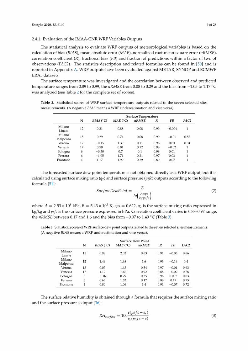
The surface temperature was investigated and the correlation between observed and predictedtemperature ranges from 0.89 to 0.99, the nRMSE from 0.08 to 0.29 and the bias from −1.05 to 1.17 ◦Cwas analyzed (see Table 2 for the complete set of scores).

Table 2. Statistical scores of WRF surface temperature outputs related to the seven selected sitesmeasurements. (A negative BIAS means a WRF underestimation and vice versa).

Surface TemperatureN BIAS (◦C) MAE (◦C) nRMSE R FB FAC2

MilanoLinate 12 0.21 0.88 0.08 0.99 −0.004 1

MilanoMalpensa 15 0.29 0.74 0.08 0.99 −0.01 0.87

Verona 17 −0.15 1.39 0.11 0.98 0.03 0.94Venezia 17 0.58 0.81 0.12 0.98 −0.02 1Bologna 6 −0.30 0.7 0.1 0.98 0.01 1Ferrara 6 −1.05 1.71 0.21 0.97 0.03 1

Frontone 4 1.17 1.99 0.29 0.89 0.07 1

The forecasted surface dew point temperature is not obtained directly as a WRF output, but it iscalculated using surface mixing ratio (q2) and surface pressure (psfc) outputs according to the followingformula [51]:

Sur f aceDewPoint =B

ln(

A∗epsq2∗ps f c

) (2)

where A = 2.53 × 108 kPa, B = 5.43 × 103 K, eps = 0.622, q2 is the surface mixing ratio expressed inkg/kg and psfc is the surface pressure expressed in hPa. Correlation coefficient varies in 0.88–0.97 range,the nRMSE between 0.17 and 1.6 and the bias from −0.07 to 1.49 ◦C (Table 3).

Table 3. Statistical scores of WRF surface dew point outputs related to the seven selected sites measurements.(A negative BIAS means a WRF underestimation and vice versa).

Surface Dew PointN BIAS (◦C) MAE (◦C) nRMSE R FB FAC2

MilanoLinate 15 0.98 2.03 0.63 0.91 −0.06 0.66

MilanoMalpensa 12 1.49 1.68 1.6 0.93 −0.19 0.4

Verona 13 0.07 1.43 0.54 0.97 −0.01 0.93Venezia 17 1.12 1.46 0.92 0.88 −0.09 0.78Bologna 6 −0.07 0.79 0.35 0.96 0.007 0.83Ferrara 6 0.63 1.62 0.17 0.88 0.17 0.75

Frontone 4 0.80 1.06 1.4 0.91 −0.07 0.72

The surface relative humidity is obtained through a formula that requires the surface mixing ratioand the surface pressure as input [36]:

RHsur f ace = 100e(ps f c− es)

es(ps f c− e)(3)

Energies 2020, 13, 6140 10 of 28

where:

• es = e0 ∗ exp(e1

t−ct−e2

),

• e = q2∗ps f ceps+q2

,

• e0 = 6.112 hPa,• e1 = 17.67,• e2 = 29.65,• eps = 0.622• c = 273.15,• q2 is the surface mixing ratio• ps f c is the surface pressure in hPa.

Concerning the surface relative humidity, the forecasts are substantially in agreement with themeasurements: Ferrara and Frontone sites are slightly underestimated whilst the remaining sites areoverestimated (Table 4).

Table 4. Statistical scores of WRF surface relative humidity outputs of the seven selected sites (a negativeBIAS means a WRF underestimation and vice versa).

Surface Relative HumidityN BIAS (%) MAE (%) nRMSE R FB FAC2

MilanoLinate 12 3.87 9.16 0.21 0.86 −0.01 1

MilanoMalpensa 15 3.28 4.63 0.09 0.98 −0.01 1

Verona 13 3.11 7.87 0.46 0.91 0.001 1Venezia 17 3.22 8.03 0.16 0.79 −0.01 1Bologna 6 0.36 1.14 0.02 0.99 −0.001 1Ferrara 6 6.5 6.5 0.13 0.92 0.02 1

Frontone 4 3.61 8.55 0.10 0.89 0.01 1

The WRF model wind output is provided as Eastward (U) and Northward (V) components in theArakawa C staggered grid [44] in which the U component refers to the center of the left grid face andthe V to the lower grid faces. These components are relative to the model grid and not to the Earthcoordinates. METAR data report wind speed and direction; hence, before comparison, U and V windvectors have been converted in wind speed. With regards to wind speed, performances are worse thanother variables, however reasonable if accounting for a systematic estimation error for all the selectedsites (Table 5).

Table 5. Statistical scores of WRF wind speed at 10 m outputs of the seven selected sites. (a negativeBIAS means a WRF underestimation and vice versa).

Wind Speed at 10 mN BIAS (m/s) MAE (m/s) nRMSE R FB FAC2

MilanoLinate 12 −0.13 0.93 1.15 0.26 0.17 0.67

MilanoMalpensa 15 −1.12 1.67 0.82 0.45 0.10 0.67

Verona 13 −0.42 1.14 0.62 0.63 0.05 0.69Venezia 17 0.39 1.16 0.72 0.70 0.18 0.41Bologna 6 −0.44 0.93 0.48 0.29 0.05 0.66Ferrara 6 1.73 1.81 1.19 0.38 −0.16 0.67

Frontone 4 −0.19 1.25 1.04 0.64 0.04 0.72

Overall, the IMAA-CNR WRF model shows good performances for the selected sites; differencesbetween observed and forecast values are accounted when tuning the thresholds of the MBFog method.

Energies 2020, 13, 6140 11 of 28

2.4.2. Definition of the Thresholds

Site-specific climatological and statistical analysis were carried out for each of the seven selectedsites in order to derive appropriate thresholds. In particular, we performed a climatologicalcharacterization of surface temperature, surface relative humidity, 10 m wind speed and surfacedew point during reported fog events, based on the historical series of METAR and SYNOP bulletinsin the period January 2011–December 2017. Threshold values are computed via a statistical methodaimed at maximizing the accuracy on the training dataset (climatological METAR and SYNOPdataset 2011–2017). Starting from this, we derived a corresponding analytical model given by:Threshold = MEAN ± STD + sign (BIAS)*MAE/2. This expression is only intended to provide aposteriori analytical reference for thresholds, explaining their order of magnitude in terms of threecontributions related to the climatological dataset (i.e., MEAN and STD) and the NWP method(i.e., MAE) used. Thus, in this expression, RH_thresh and WS_min_thresh are set to the averageminus the standard deviation values while TDepr_thresh and WS_max_thresh to the average plusthe standard deviation values. These thresholds should be adapted considering the BIAS and theMAE of the WRF outputs presented above (see Section 2.4.1). All of them should be increased orreduced (depending on the BIAS sign) by a quantity equal to the half of the MAE. Regarding therelative humidity difference between the first two vertical levels (RHDiff) and the fog stability index,historical series are not available. Thus, in the case of RHDiff, we selected a threshold available andvalidated in literature, equal to −4.5% [39], while for the FSI we selected a subset of WRF outputs toderive an appropriate threshold. To this aim, we use the maximization criteria based on the area underROC (receiving operating characteristic) curve and Youden’s index [52]. Youden’s index expresses theperformances of a dichotomous diagnostic test (see Appendix B). We calculated this index using fixedvalues for relative humidity, surface temperature, surface dew point and wind speed thresholds butvarying the FSI threshold value between its minimum and maximum value (0 and 100, assumed to bethe highest and lowest probability of fog occurrence, respectively). The appropriate FSI_thresh waschosen as the FSI value corresponding to the maximum Youden’s index. This permitted us to obtainthe maximum area under ROC curve (AROC).

3. Results and Discussion

In this section, we report results of the site by site analysis. This is conducted to customize the fogforecasting method to the specific environment, in terms of values assumed by the variables of interestin the presence of fog and the relative derived thresholds.

3.1. Milano Linate (45.46143 N, 9.2626 E, 103 m a.s.l.)

Milano Linate is situated in the Po Valley and is characterized by a relative high probability of fogformation. This is confirmed by METAR and SYNOP 2011–2017 observations: during the whole period,fog has been reported in 5311 of 122075 measurements (4.33% of total observations number) distributedunequally in all seasons: 51.16% in autumn, 46.96% in winter, 1.73% in spring and 0.15% in summer.Values and selected thresholds are reported in Table 6, while Figure 5 shows the related histograms ofmeasurements. It should be noted that METAR ambient and dew point temperatures are roundedtowards the nearest integer, causing unrealistic gaps when T is close to Td and consequently in fogcases. This limitation has an impact also in relative humidity values that are obtained from the ambientand dew point temperatures [36]. Therefore, we used SYNOP data for the ambient temperature,dew point temperature and relative humidity climatological analysis in all the evaluated sites.

According to Youden’s index, FSI_thresh equals 28, obtaining the ROC curve in Figure 5d,with AROC = 0.72. By applying these thresholds to the IMAA-CNR WRF variables outputs, the MBFogmethod has been evaluated against METAR, achieving the following performances: POD = 0.70,FAR = 0.12 and Accuracy = 0.94.

Energies 2020, 13, 6140 12 of 28

Table 6. Mean, standard deviation and thresholds selected for relative humidity, surface temperature/dewpoint depression and wind speed measured in fog condition and FSI threshold calculated usingYouden’s index for Milano Linate.

Mean Standard Deviation Threshold

RH 99.30% 3.40% Min: 98%Diff_T_TDEW 0.10 ◦C 0.21 ◦C Max: 1.2 ◦C

WS10 1.43 m/s 0.75 m/s Min: 0 m/sMax: 1.3 m/s

FSI - - 28


Table 6. Mean, standard deviation and thresholds selected for relative humidity, surface tempera-ture/dew point depression and wind speed measured in fog condition and FSI threshold calculated using Youden’s index for Milano Linate.

Mean Standard Deviation Threshold RH 99.30% 3.40% Min: 98%

Diff_T_TDEW 0.10 °C 0.21 °C Max: 1.2 °C

WS10 1.43 m/s 0.75 m/s Min: 0 m/s

Max: 1.3 m/s FSI - - 28

(a) (b)

(c) (d)

Figure 5. Histograms of the measurements of (a) relative humidity, (b) surface temperature/dew point difference, (c) wind speed in fog condition at Milano Linate in the period January 2011–December 2017 and (d) receiving operating characteristic (ROC) curve with FSI_thresh = 28.

According to Youden’s index, FSI_thresh equals 28, obtaining the ROC curve in Figure 5d, with AROC = 0.72. By applying these thresholds to the IMAA-CNR WRF variables outputs, the MBFog method has been evaluated against METAR, achieving the following performances: POD = 0.70, FAR = 0.12 and Accuracy = 0.94.

Figure 5. Histograms of the measurements of (a) relative humidity, (b) surface temperature/dew pointdifference, (c) wind speed in fog condition at Milano Linate in the period January 2011–December 2017and (d) receiving operating characteristic (ROC) curve with FSI_thresh = 28.

3.2. Milano Malpensa (45.62 N, 8.7231 E, 211 m a.s.l.)

The METAR 2011–2017 observations at Milano Malpensa reported fog in 2797 out of 121987cases (2.29% of total observations) occurring in autumn (42.97%), winter (56.67%), spring (0.25%) andsummer (0.15%), respectively. The mean and the standard deviation of the surface relative humidity(RH), the difference between surface temperature and surface dew point (Diff_T_TDEW) and the windspeed at 10 m (WS10) have also been calculated. Values and adapted thresholds are reported in Table 7while Figure 6 shows the related histogram of measurements.

Energies 2020, 13, 6140 13 of 28

Table 7. Mean, standard deviation and thresholds selected for relative humidity, surface temperature/dewpoint depression and wind speed measured in fog condition and fog stability index (FSI) thresholdcalculated using Youden’s index for Milano Malpensa.




FSI - - 26


3.2. Milano Malpensa (45.62 N, 8.7231 E, 211 m a.s.l.)

The METAR 2011–2017 observations at Milano Malpensa reported fog in 2797 out of 121987 cases (2.29% of total observations) occurring in autumn (42.97%), winter (56.67%), spring (0.25%) and summer (0.15%), respectively. The mean and the standard deviation of the surface relative humidity (RH), the difference between surface temperature and surface dew point (Diff_T_TDEW) and the wind speed at 10 m (WS10) have also been calculated. Values and adapted thresholds are reported in Table 7 while Figure 6 shows the related histogram of measurements.

Table 7. Mean, standard deviation and thresholds selected for relative humidity, surface tempera-ture/dew point depression and wind speed measured in fog condition and fog stability index (FSI) threshold calculated using Youden’s index for Milano Malpensa.



WS10 1.07 m/s 0.68 m/s Min: 0 m/s

Max: 1.3 m/s FSI - - 26

(a) (b)

(c) (d)

Figure 6. Histograms of the measurements of (a) relative humidity, (b) surface temperature/dew point difference, (c) wind speed in fog condition at Milano Malpensa in the period January 2011–December 2017 and (d) ROC curve with FSI_thresh = 26.

Figure 6. Histograms of the measurements of (a) relative humidity, (b) surface temperature/dew pointdifference, (c) wind speed in fog condition at Milano Malpensa in the period January 2011–December 2017and (d) ROC curve with FSI_thresh = 26.

According to Youden’s index, FSI_thresh equals 26, obtaining the ROC curve in Figure 6d,with AROC = 0.71. By applying these thresholds to the IMAA-CNR WRF variables outputs, the MBFogmethodology has been evaluated against METAR, achieving the following performances: POD = 0.88,FAR = 0.30 and Accuracy = 0.97.

3.3. Verona (45.3875 N, 10.8723 E, 68 m a.s.l.)

Verona is situated in the Po Valley next to Lake Garda. Its location is favorable for fog, and thenear water basin represents a further source. Indeed, METAR during years 2011–2017 reports fog in5.25% of measurements (6447 out of 118790). Among these, 50.58% are in winter, 46.01% in autumn,

Energies 2020, 13, 6140 14 of 28

3.12% in spring and 0.29% in summer. Histograms and values for this site are reported in Figure 7 andTable 4.


According to Youden’s index, FSI_thresh equals 26, obtaining the ROC curve in Figure 6d, with AROC = 0.71. By applying these thresholds to the IMAA-CNR WRF variables outputs, the MBFog methodology has been evaluated against METAR, achieving the following performances: POD = 0.88, FAR = 0.30 and Accuracy = 0.97.

3.3. Verona (45.3875 N, 10.8723 E, 68 m a.s.l.)

Verona is situated in the Po Valley next to Lake Garda. Its location is favorable for fog, and the near water basin represents a further source. Indeed, METAR during years 2011–2017 reports fog in 5.25% of measurements (6447 out of 118790). Among these, 50.58% are in winter, 46.01% in autumn, 3.12% in spring and 0.29% in summer. Histograms and values for this site are reported in Figure 7 and Table 4.

(a) (b)

(c) (d)

Figure 7. Histograms of the measurements of (a) relative humidity, (b) surface temperature/dew point difference, (c) wind speed in fog condition at Verona in the period January 2011–December 2017 and (d) ROC curve with FSI_thresh = 26.

In Figure 7, it is shown that the ROC curve obtained with an FSI threshold of 26 underlies an AROC of 0.72. With the thresholds reported in Table 8, MBFog forecast method achieves the follow-ing performances: POD = 0.80, FAR = 0.14 and Accuracy = 0.96.

Figure 7. Histograms of the measurements of (a) relative humidity, (b) surface temperature/dew pointdifference, (c) wind speed in fog condition at Verona in the period January 2011–December 2017 and(d) ROC curve with FSI_thresh = 26.

In Figure 7, it is shown that the ROC curve obtained with an FSI threshold of 26 underlies anAROC of 0.72. With the thresholds reported in Table 8, MBFog forecast method achieves the followingperformances: POD = 0.80, FAR = 0.14 and Accuracy = 0.96.

Table 8. Mean, standard deviation and thresholds selected for relative humidity, surface temperature/dewpoint depression and wind speed measured in fog condition and FSI threshold calculated using Youden’sindex for Verona.




FSI - - 26

3.4. Venezia (45.5053 N, 12.3519 E, 68 m a.s.l.)

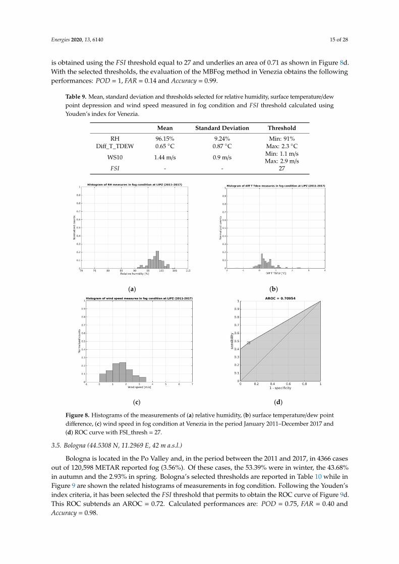
The METAR 2011–2017 reports indicate the presence of fog in 4477 out of 120,877 cases (3.65% ofthe total observations). Of these, the 50.70% are in winter, 43.36% in autumn, 4.89% in spring and2.14% in summer. Table 9 and Figure 8 report values and histograms for Venezia. The ROC curve

Energies 2020, 13, 6140 15 of 28

is obtained using the FSI threshold equal to 27 and underlies an area of 0.71 as shown in Figure 8d.With the selected thresholds, the evaluation of the MBFog method in Venezia obtains the followingperformances: POD = 1, FAR = 0.14 and Accuracy = 0.99.

Table 9. Mean, standard deviation and thresholds selected for relative humidity, surface temperature/dewpoint depression and wind speed measured in fog condition and FSI threshold calculated usingYouden’s index for Venezia.



WS10 1.44 m/s 0.9 m/s Min: 1.1 m/sMax: 2.9 m/s

FSI - - 27


Table 8. Mean, standard deviation and thresholds selected for relative humidity, surface tempera-ture/dew point depression and wind speed measured in fog condition and FSI threshold calculated using Youden’s index for Verona.



WS10 1.01 m/s 0.84 m/s Min: 0 m/s

Max: 1.3 m/s FSI - - 26

3.4. Venezia (45.5053 N, 12.3519 E, 68 m a.s.l.)

The METAR 2011–2017 reports indicate the presence of fog in 4477 out of 120,877 cases (3.65% of the total observations). Of these, the 50.70% are in winter, 43.36% in autumn, 4.89% in spring and 2.14% in summer. Table 9 and Figure 8 report values and histograms for Venezia. The ROC curve is obtained using the FSI threshold equal to 27 and underlies an area of 0.71 as shown in Figure 8d. With the selected thresholds, the evaluation of the MBFog method in Venezia obtains the following performances: POD = 1, FAR = 0.14 and Accuracy = 0.99.

Table 9. Mean, standard deviation and thresholds selected for relative humidity, surface tempera-ture/dew point depression and wind speed measured in fog condition and FSI threshold calculated using Youden’s index for Venezia.



WS10 1.44 m/s 0.9 m/s Min: 1.1 m/s Max: 2.9 m/s

FSI - - 27

(a) (b)


(c) (d)

Figure 8. Histograms of the measurements of (a) relative humidity, (b) surface temperature/dew point difference, (c) wind speed in fog condition at Venezia in the period January 2011–December 2017 and (d) ROC curve with FSI_thresh = 27.

3.5. Bologna (44.5308 N, 11.2969 E, 42 m a.s.l.)

Bologna is located in the Po Valley and, in the period between the 2011 and 2017, in 4366 cases out of 120,598 METAR reported fog (3.56%). Of these cases, the 53.39% were in winter, the 43.68% in autumn and the 2.93% in spring. Bologna’s selected thresholds are reported in Table 10 while in Fig-ure 9 are shown the related histograms of measurements in fog condition. Following the Youden’s index criteria, it has been selected the FSI threshold that permits to obtain the ROC curve of Figure 9d. This ROC subtends an AROC = 0.72. Calculated performances are: POD = 0.75, FAR = 0.40 and Accuracy = 0.98.

Table 10. Mean, standard deviation and thresholds selected for relative humidity, surface tempera-ture/dew point depression and wind speed measured in fog condition and FSI threshold calculated using Youden’s index for Bologna.




FSI - - 24

(a) (b)

Figure 8. Histograms of the measurements of (a) relative humidity, (b) surface temperature/dew pointdifference, (c) wind speed in fog condition at Venezia in the period January 2011–December 2017 and(d) ROC curve with FSI_thresh = 27.

3.5. Bologna (44.5308 N, 11.2969 E, 42 m a.s.l.)

Bologna is located in the Po Valley and, in the period between the 2011 and 2017, in 4366 casesout of 120,598 METAR reported fog (3.56%). Of these cases, the 53.39% were in winter, the 43.68%in autumn and the 2.93% in spring. Bologna’s selected thresholds are reported in Table 10 while inFigure 9 are shown the related histograms of measurements in fog condition. Following the Youden’sindex criteria, it has been selected the FSI threshold that permits to obtain the ROC curve of Figure 9d.This ROC subtends an AROC = 0.72. Calculated performances are: POD = 0.75, FAR = 0.40 andAccuracy = 0.98.

Energies 2020, 13, 6140 16 of 28

Table 10. Mean, standard deviation and thresholds selected for relative humidity, surface temperature/dewpoint depression and wind speed measured in fog condition and FSI threshold calculated using Youden’sindex for Bologna.




FSI - - 24


(c) (d)

Figure 8. Histograms of the measurements of (a) relative humidity, (b) surface temperature/dew point difference, (c) wind speed in fog condition at Venezia in the period January 2011–December 2017 and (d) ROC curve with FSI_thresh = 27.

3.5. Bologna (44.5308 N, 11.2969 E, 42 m a.s.l.)

Bologna is located in the Po Valley and, in the period between the 2011 and 2017, in 4366 cases out of 120,598 METAR reported fog (3.56%). Of these cases, the 53.39% were in winter, the 43.68% in autumn and the 2.93% in spring. Bologna’s selected thresholds are reported in Table 10 while in Fig-ure 9 are shown the related histograms of measurements in fog condition. Following the Youden’s index criteria, it has been selected the FSI threshold that permits to obtain the ROC curve of Figure 9d. This ROC subtends an AROC = 0.72. Calculated performances are: POD = 0.75, FAR = 0.40 and Accuracy = 0.98.

Table 10. Mean, standard deviation and thresholds selected for relative humidity, surface tempera-ture/dew point depression and wind speed measured in fog condition and FSI threshold calculated using Youden’s index for Bologna.




FSI - - 24

(a) (b)


(c) (d)

Figure 9. Histograms of the measurements of (a) relative humidity, (b) surface temperature/dew point difference, (c) wind speed in fog condition at Bologna in the period January 2011–December 2017 and (d) ROC curve obtained with FSI_thresh = 24.

3.6. Ferrara (44.8156 N, 11.6125 E, 10 m a.s.l.)

Ferrara, situated in the middle of Po Valley, is characterized by high frequency of fog occurrence, as reported in 2565 out of 32866 cases, i.e., 7.84% (the 41.92% during winter, the 53.7% in autumn, the 3.64% during spring and the 0.74% during summer) in the METAR 2011–2017 observations. Histo-grams and selected values for this site are reported in Figure 10 and Table 11.

(a) (b)

(c) (d)

Figure 10. Histograms of the measurements of (a) relative humidity, (b) surface temperature/dew point difference, (c) wind speed in fog condition at Ferrara in the period January 2011–December 2017 and (d) ROC curve obtained with FSI_thresh = 25.

Figure 9. Histograms of the measurements of (a) relative humidity, (b) surface temperature/dew pointdifference, (c) wind speed in fog condition at Bologna in the period January 2011–December 2017 and(d) ROC curve obtained with FSI_thresh = 24.

3.6. Ferrara (44.8156 N, 11.6125 E, 10 m a.s.l.)

Ferrara, situated in the middle of Po Valley, is characterized by high frequency of fog occurrence,as reported in 2565 out of 32866 cases, i.e., 7.84% (the 41.92% during winter, the 53.7% in autumn,the 3.64% during spring and the 0.74% during summer) in the METAR 2011–2017 observations.Histograms and selected values for this site are reported in Figure 10 and Table 11.

In Figure 10d, the ROC curve is shown, obtained with FSI threshold equal to 25 with an AROC of0.74. Applying the thresholds reported in Table 12, the MBFog method achieves for Ferrara POD = 0.65,FAR = 0.08 and Accuracy = 0.90.

Energies 2020, 13, 6140 17 of 28


(c) (d)

Figure 9. Histograms of the measurements of (a) relative humidity, (b) surface temperature/dew point difference, (c) wind speed in fog condition at Bologna in the period January 2011–December 2017 and (d) ROC curve obtained with FSI_thresh = 24.

3.6. Ferrara (44.8156 N, 11.6125 E, 10 m a.s.l.)

Ferrara, situated in the middle of Po Valley, is characterized by high frequency of fog occurrence, as reported in 2565 out of 32866 cases, i.e., 7.84% (the 41.92% during winter, the 53.7% in autumn, the 3.64% during spring and the 0.74% during summer) in the METAR 2011–2017 observations. Histo-grams and selected values for this site are reported in Figure 10 and Table 11.

(a) (b)

(c) (d)

Figure 10. Histograms of the measurements of (a) relative humidity, (b) surface temperature/dew point difference, (c) wind speed in fog condition at Ferrara in the period January 2011–December 2017 and (d) ROC curve obtained with FSI_thresh = 25.

Figure 10. Histograms of the measurements of (a) relative humidity, (b) surface temperature/dew pointdifference, (c) wind speed in fog condition at Ferrara in the period January 2011–December 2017 and(d) ROC curve obtained with FSI_thresh = 25.

Table 11. Mean, standard deviation and thresholds selected for relative humidity, surface temperature/dewpoint depression and wind speed measured in fog condition and FSI threshold calculated using Youden’sindex for Ferrara.


RH 92.98% 4.75% Min: 91%Diff_T_TDEW 1.07 ◦C 0.75 ◦C Max: 1 ◦C


FSI - - 25

Table 12. Mean, standard deviation and thresholds selected for relative humidity, surface temperature/dewpoint depression and wind speed measured in fog condition and FSI threshold calculated using Youden’sindex for Frontone.




FSI - - 32

3.7. Frontone (43.5169 N, 12.7277 E, 574 m a.s.l.)

Frontone is located in the Apennines, in a small valley favorable to the development of radiationfog mainly during autumn and winter seasons. METAR 2011–2017 reported it in 2906 out of 60,125 cases(the 4.71%) distributed during the different seasons in this way: 39.82% in winter, 41.38% in autumn,14.96% in spring and 3.84% in summer.

Energies 2020, 13, 6140 18 of 28

Values and selected thresholds for this site are reported in Table 12, while in Figure 11 there areshown the related histogram of measurements in fog condition. With these thresholds, we obtainedPOD = 1, FAR = 0.08 and Accuracy = 0.97.


Table 11. Mean, standard deviation and thresholds selected for relative humidity, surface tempera-ture/dew point depression and wind speed measured in fog condition and FSI threshold calculated using Youden’s index for Ferrara.


Diff_T_TDEW 1.07 °C 0.75 °C Max: 1 °C


FSI - - 25

In Figure 10d, the ROC curve is shown, obtained with FSI threshold equal to 25 with an AROC of 0.74. Applying the thresholds reported in Table 12, the MBFog method achieves for Ferrara POD = 0.65, FAR = 0.08 and Accuracy = 0.90.

3.7. Frontone (43.5169 N, 12.7277 E, 574 m a.s.l.)

Frontone is located in the Apennines, in a small valley favorable to the development of radiation fog mainly during autumn and winter seasons. METAR 2011–2017 reported it in 2906 out of 60,125 cases (the 4.71%) distributed during the different seasons in this way: 39.82% in winter, 41.38% in autumn, 14.96% in spring and 3.84% in summer.

Values and selected thresholds for this site are reported in Table 12, while in Figure 11 there are shown the related histogram of measurements in fog condition. With these thresholds, we obtained POD = 1, FAR = 0.08 and Accuracy = 0.97.

(a) (b)

(c) (d)

Figure 11. Histograms of the measurements of (a) relative humidity, (b) surface temperature/dew point difference, (c) wind speed in fog condition at Frontone in the period January 2011–December 2017 and (d) ROC curve obtained with FSI_thresh = 32.

Figure 11. Histograms of the measurements of (a) relative humidity, (b) surface temperature/dew pointdifference, (c) wind speed in fog condition at Frontone in the period January 2011–December 2017 and(d) ROC curve obtained with FSI_thresh = 32.

For the Frontone site, the ROC curve was obtained using an FSI threshold equal to 32 and underliesan area of 0.81 (see Figure 11d).

3.8. Discussion of MBFog Evaluation Results

MBFog performances were evaluated with respect to the following methods:

(a) Fog Stability Index under a fixed threshold (31), as reported in [38] (i.e., FSI test);(b) RH larger than a fixed threshold (90%) and Wind Speed smaller than a fixed threshold (2 ms−1),

as reported in [34] (i.e., RH/Wind test);(c) Visibility obtained from Liquid Water Content (LWC) using Kunkel’s law [41] less than a fixed

threshold (1 km), as reported in [37,41] (i.e., Visibility test).

Note that all variables used in these comparisons (surface temperature, surface dew pointtemperature, wind speed at 10 m, temperature at 850 hPa, wind speed at 850 hPa and surface mixingratio) are obtained from the same IMAA-CNR WRF runs used in MBFog performance evaluation,i.e., daytime hourly outputs of 35 runs selected in the period January–April 2018. In this framework,(see the Appendix C for all statistical scores), MBFog results in better performances with respect to theother methods mentioned above. This is mainly attributed to the fact that the thresholds are specificallytuned for each site. The evaluation has been carried out against METAR data on seven sites chosen fortheir frequent fog occurrence in the period January–April 2018.

Table 13 contains the overall statistical scores for all the sites. Appendix B explains the definitionsof the considered statistical indexes (see [50] for more details).

Energies 2020, 13, 6140 19 of 28

Table 13. Overall statistic performances of multitest fog forecast method for the selected sites.

Milano Linate Milano Malpensa Verona Venezia Bologna Ferrara Frontone

tp 14 7 12 11 3 22 12tn 119 109 104 122 127 104 16fp 2 3 2 2 2 2 1fn 6 1 3 0 1 12 0

n_total 141 120 121 136 133 140 29Accuracy 0.94 0.97 0.96 0.99 0.98 0.90 0.97

BIAS 0.80 1.25 0.93 1.17 1.25 0.71 1.08POD 0.70 0.88 0.80 1 0.75 0.65 1FAR 0.12 0.30 0.14 0.14 0.40 0.08 0.08

POFD 0.02 0.03 0.02 0.02 0.02 0.02 0.06SR 0.88 0.70 0.86 0.86 0.60 0.92 0.92TS 0.64 0.64 0.71 0.86 0.50 0.61 0.92

ETS 0.59 0.61 0.67 0.84 0.49 0.54 0.87HKD 0.68 0.85 0.78 0.98 0.73 0.63 0.94HSS 0.75 0.76 0.80 0.91 0.66 0.70 0.93

ORSS 0.99 0.99 0.99 1 0.99 0.98 1

In the evaluated sites, MBFog forecast method is able to predict fog in the 6–30 h after the WRFstart time with an average accuracy of 0.96, an average probability of detection of 0.83 and an averagefalse alarm ratio of 0.18. The average success ratio is 0.82; this means that the 82% of the fog forecastedhave been actually observed. The goodness of the MBFog method has been evaluated with respect tothe random chance by means of the odds ratio skill score obtaining average value of 0.994 (1 being theperfect score). MBFog suffers from a relatively high false alarm ratio (average value of 0.18); this meansthat the algorithm can produce a false underestimation of the irradiance reaching the photovoltaicpanels when fog is expected while it does not occur.

Considering similar fog forecasting methods, in [40], an accuracy of 0.95 has been reported. In [34],the implemented multivariable-based diagnostic method scored an ETS = 0.334, while the single-rulemethodology (LWC rule) scored an ETS = 0.063. Comparison against these methods [34,39] revealsthat MBFog is aligned in terms of performances (average accuracy 0.96, average ETS = 0.409); however,it also reveals that this class of fog forecast methods experiences similar limitations, e.g., they predictfog formation fairly well, but they do not predict its duration as well.

3.9. First Results of the Application of the Fog Postprocessing Layer to the IMAA-CNR WRF Irradiance Forecast

In this subsection, we present a first evaluation of the application of the fog postprocessing layerto the WRF global horizontal irradiance forecast.

First of all, we selected those case in which IMAA-CNR WRF did not predicted fog while it occurs,after that we calculated statistical scores for 4 METAR site we have available the measured GHI valuesin the period between January and April 2018: Milano Linate, Milano Malpensa, Bologna e Ferrara.WRF GHI scores have been calculated in both the cases in which fog postprocessing layer is appliedor not. In all the considered cases, we had an improvement of the statistical scores when using fogpostprocessing layer, as reported in Table 14 below.

Table 14. Comparison of GHI WRF output performances with or without the application of fogpostprocessing layer (ppl).

Milano Linate Milano Malpensa Bologna FerraraNo fog ppl With fog ppl No fog ppl With fog ppl No fog ppl With fog ppl No fog ppl With fog ppl

n_total 23 23 15 15 14 14 41 41BIAS (W·m−2) 89.44 23.49 80.98 49.42 88.62 26.02 82.73 17.60MAE (W·m−2) 89.96 31.11 80.98 49.42 88.62 27.12 102.12 44.03

RMSE (W·m−2) 122.68 39.97 118.58 76.4 125.47 36.36 139.28 59.89R 0.83 0.96 0.80 0.86 0.79 0.98 0.63 0.80

FB −0.15 −0.05 −0.25 −0.20 −0.14 −0.05 −0.14 −0.04nMSE 0.45 0.06 1.22 0.63 0.46 0.05 0.70 0.19FAC2 0.52 0.78 0.13 0.27 0.36 0.93 0.56 0.73

Energies 2020, 13, 6140 20 of 28

4. Conclusions

This work presents a multitest method to forecast the presence of fog using the output data ofa numerical weather prediction model, namely WRF. The fog forecast method is based on severalthreshold tests applied to the main meteorological variables involved in fog processes obtained fromthe WRF NWP model at spatial resolution of 3 km and temporal resolution of 1 h over the Italianpeninsula. The implemented method combines several deterministic tests in which meteorologicalvariables involved in the fog process and the fog stability index (FSI) are evaluated with respect toempirical site-specific thresholds. The evaluation has been carried out against METAR data on sevensites chosen for their frequent fog occurrence in the period January–April 2018.

The MBFog method tends to maximize the accuracy and the probability of detection and atthe same time to minimize the probability of false detection and the probability of false alarm withrespect to single-test methods for the evaluated dataset. The strength of this method is its capabilityto adapt the thresholds to the specific site under investigation. This means that, if meteorologicaltime series are available, the method can be adapted for other sites after a preliminary meteorologicaland climatological analysis. The output of the proposed fog forecast method can activate or not aspecific fog postprocessing layer designed to correct the global horizontal irradiance forecasted by theWRF model in order to optimize the forecast of the irradiance reaching the PV panels surface. We canconclude that the proposed MBFog method is useful to forecast fog occurrence, and thus it can be usedto improve the forecast of PV power production.

Author Contributions: Conceptualization, D.C., D.G. and F.R.; data curation, F.D.P., S.L., E.R. (Elisabetta Ricciardelli)and E.R. (Ermann Ripepi); formal analysis, S.T.N., D.C., D.G., S.G. and E.R. (Elisabetta Ricciardelli);funding acquisition, E.G.; investigation, E.R. (Elisabetta Ricciardelli); Methodology, S.T.N.; project administration,E.G. and F.R.; resources, S.G., E.R. (Ermann Ripepi) and M.V.; software, S.T.N. and F.D.P.; supervision, F.R.;validation, D.C., D.G. and F.R.; visualization, S.T.N.; writing—original draft, S.T.N.; writing—review and editing,D.C., F.D.P., D.G., S.G., E.G., S.L., E.R. (Elisabetta Ricciardelli), E.R. (Ermann Ripepi), M.V. and F.R. All authorshave read and agreed to the published version of the manuscript.

Funding: This work was financed by the Italian Ministry of Economic Development (MISE) in the framework ofthe SolarCloud project, contract No. B01/0771/04/X24.

Acknowledgments: We acknowledge the Italian Air Force Meteorological Service for the kind cooperation inproviding us METAR reports and SYNOP bulletins used in this work. We are also grateful to Claudia Faccaniand Gianluca Tisselli from the Italian air navigation service provider (ENAV) for their valuable support in thedefinition of the measurement dataset.

Conflicts of Interest: The authors declare no conflict of interest. The founding sponsors had no role in the designof the study; in the collection, analyses, or interpretation of data; in the writing of the manuscript and in thedecision to publish the results.

List of Abbreviations

AROC Area under Receiving Operating CharacteristicDEM Digital Elevation ModelDiff_T_TDEW Surface temperature/dew point depression (◦C)ECMWF European Centre for Medium-Range Weather ForecastsERA5 HRES Fifth generation ECMWF atmospheric ReAnalysis High RESolutionFSI Fog Stability Index (-)GHI Global Horizontal Irradiance (W·m−2)GFS Global Forecast SystemLWC Liquid Water Content (g·kg−1)MBFog Multitest-Based method for Fog forecastingMETAR METeorological Aerodrome ReportMODIS MODerate resolution Imaging SpectroradiometerMM5 Fifth-Generation NCAR/Penn State Mesoscale Model

Energies 2020, 13, 6140 21 of 28

NCAR National Center for Atmospheric ResearchNWP Numerical Weather Predictionpsfc Surface pressure (hPa)q2 Surface mixing ration (kg·kg−1)RH Relative Humidity (%)ROC Receiving Operating CharacteristicSYNOP Surface SYNOPtic observationsT850 Temperature at 850 hPa (K)Td Surface dew point temperature (K)Ts Surface temperature (K)WMO World Meteorological OrganizationWRF Weather Research and ForecastWS10 Wind speed at 10 m (m·s−1)WS850 Wind speed at 850 hPa (m·s−1)

Appendix A. Standard Verification Methods for Continuous Variables Forecasts

In this appendix we describe the statistical indexes used for the validation of the WRF outputs forecasts: bias,mean absolute error (MAE), normalized root-mean-square error (nRMSE), correlation coefficient (R), fractional bias(FB), normalized mean square error (nMSE), fraction of predictions within a factor of two of observations (FAC2).

• Bias

Bias is defined as the sum of the difference between forecasted (F) and observed (O) values divided by thetotal number of samples.

BIAS =1N

N∑i=1

Fi −Oi (A1)

Bias gives an indication of the forecast average error but does not measure the correspondence betweenforecasts and observations. Bias can assume values between −∞ and +∞, perfect score means a bias equal to zero.

• Mean Absolute Error

Mean Absolute Error (MAE) is the ratio between the sum of the absolute value of the difference betweenforecasts (F) and observations (O) and the total number of samples.

MAE =1N

N∑i=1

|Fi −Oi| (A2)

It is used to address the average magnitude of the forecast errors but does not indicate the direction of them.It can be a value between zero and +∞with perfect score zero.

• Normalized Root-Mean-Square Error

Normalized Root-Mean-Square Error (nRMSE) is calculated according to the following formula:

nRMSE =

√1N

∑Ni=1(Fi −Oi)

2

1N

∑Ni=1 Oi

(A3)

It measures average error weighted according to the square of the error and is normalized by the meanobservation value. In particular this index is influenced mainly by large errors encouraging conservative forecasts.It can assume values between 0 and 1 with perfect score 0.

• Correlation coefficient

Correlation coefficient is calculated using the following equation:

R =

∑Ni=1

(F− F

)(O− O

)√∑(

F− F)2

√∑(O− O

)2(A4)

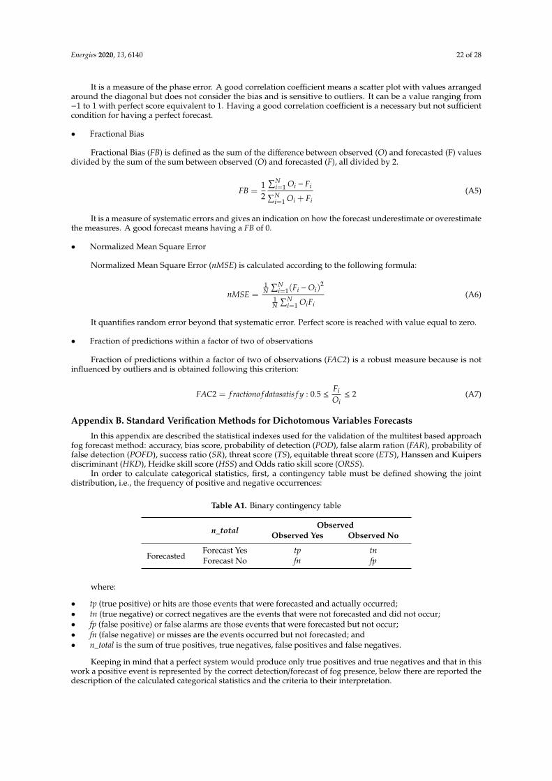
Energies 2020, 13, 6140 22 of 28

It is a measure of the phase error. A good correlation coefficient means a scatter plot with values arrangedaround the diagonal but does not consider the bias and is sensitive to outliers. It can be a value ranging from−1 to 1 with perfect score equivalent to 1. Having a good correlation coefficient is a necessary but not sufficientcondition for having a perfect forecast.

• Fractional Bias

Fractional Bias (FB) is defined as the sum of the difference between observed (O) and forecasted (F) valuesdivided by the sum of the sum between observed (O) and forecasted (F), all divided by 2.

FB =12

∑Ni=1 Oi − Fi∑Ni=1 Oi + Fi

(A5)

It is a measure of systematic errors and gives an indication on how the forecast underestimate or overestimatethe measures. A good forecast means having a FB of 0.

• Normalized Mean Square Error

Normalized Mean Square Error (nMSE) is calculated according to the following formula:

nMSE =1N

∑Ni=1(Fi −Oi)

2

1N

∑Ni=1 OiFi

(A6)

It quantifies random error beyond that systematic error. Perfect score is reached with value equal to zero.

• Fraction of predictions within a factor of two of observations

Fraction of predictions within a factor of two of observations (FAC2) is a robust measure because is notinfluenced by outliers and is obtained following this criterion:

FAC2 = f ractiono f datasatis f y : 0.5 ≤FiOi≤ 2 (A7)

Appendix B. Standard Verification Methods for Dichotomous Variables Forecasts

In this appendix are described the statistical indexes used for the validation of the multitest based approachfog forecast method: accuracy, bias score, probability of detection (POD), false alarm ration (FAR), probability offalse detection (POFD), success ratio (SR), threat score (TS), equitable threat score (ETS), Hanssen and Kuipersdiscriminant (HKD), Heidke skill score (HSS) and Odds ratio skill score (ORSS).

In order to calculate categorical statistics, first, a contingency table must be defined showing the jointdistribution, i.e., the frequency of positive and negative occurrences:

Table A1. Binary contingency table

n_totalObserved

Observed Yes Observed No

ForecastedForecast Yes tp tnForecast No fn fp

where:

• tp (true positive) or hits are those events that were forecasted and actually occurred;• tn (true negative) or correct negatives are the events that were not forecasted and did not occur;• fp (false positive) or false alarms are those events that were forecasted but not occur;• fn (false negative) or misses are the events occurred but not forecasted; and• n_total is the sum of true positives, true negatives, false positives and false negatives.

Keeping in mind that a perfect system would produce only true positives and true negatives and that in thiswork a positive event is represented by the correct detection/forecast of fog presence, below there are reported thedescription of the calculated categorical statistics and the criteria to their interpretation.

Energies 2020, 13, 6140 23 of 28

• Accuracy

Accuracy, or fraction correct, is the ratio between the sum of hits and correct negatives and the n_total. It canassume values ranging from 0 to 1 (best value). Accuracy gives the fraction of the overall correct forecasts.

Accuracy =tp + tnntotal

(A8)

• Bias score

Bias score, also called frequency bias, measures the ratio of the frequency of forecasts to the frequency ofobservations. Can assume values over zero (perfect score is 1). If BIAS < 1 the system has a tendency of underforecast, the opposite if BIAS > 1.

BIAS =tp + f ptp + f n

(A9)

• Probability of detection (POD)

Probability of detection (or true positive rate or sensitivity) returns the frequency of observed event correctlyforecasted. Values ranges from 0 to 1 with 1 perfect score. POD is sensitive to hits but not consider false alarms.

POD =tp

tp + f n(A10)

• True negative rate (Specificity)

True negative rate (or specificity) is the ratio of the true negative by the sum of all negative observed events. It isuseful in the determination of ROC (Receiving Operating Characteristic) curve and to calculate the Youden’s index.

speci f icity =tn

tn + f p(A11)

• False alarm ratio (FAR)

False alarm ratio gives an indication on the fraction of positive predicted events actually not occurred. It canassume values between 0 to 1 with 0 perfect score. It is sensitive to false alarms but not to misses.

FAR =f p

tp + f p(A12)

• Probability of false detection (POFD)

Probability of false detection (or false alarm rate) is the fraction correct negatives event not forecasted. Valuesranges from 0 to 1. POFD should be 0 in a perfect system.

POFD =f p

f p + tn(A13)

• Success ratio (SR)

Success ratio measures the fraction of hits among all the positive forecasts (sum of hits and false alarms). SR isequal to 1 − FAR. Value range is between 0 and 1, with 1 best performance indicator.

SR =tp

tp + f p(A14)

• Threat score (TS)

Threat score (or critical success index-CSI-) is the measurement of the fraction of observed and forecastedevents that were correctly predicted. Thus, it differs from the accuracy because it does not consider true negatives.It is sensitive to hits, A TS of 0 indicates that the system has no skill while 1 that system is perfect.

TS =tp

tp + f n + f p(A15)

Energies 2020, 13, 6140 24 of 28

• Equitable threat score (ETS)

Equitable threat score (or Gilbert skill score-GSS-) gives information on how well the positive forecastscorrespond to the positive observations adjusted for hits associated with random chance. It is sensitive to hits anddoes not distinguish the source of forecast error because it penalizes both misses and false alarms. It assumesvalues ranging from −1/3 to 1 with 0 and 1 respectively the worst and the best values.

ETS =tp− tprnd

tp + f n + f p + tprnd(A16)

where

tprnd =(tp + f n)(tp + f p)

ntotal(A17)

• Hansen and Kuipers discriminant (HKD)

Hansen and Kuipers discriminant (also called true skill statistic-TSS-or Peirce’s skill score-PSS-) measures ifand how well the system is able to separate positive from negative forecasts. It can be seen also as the differencebetween POD and POFD and interpreted as the sum of accuracy for events and accuracy for no events minus one.It ranges from −1 to 1, 0 indicates no skills and 1 the perfect score.

HKD =tp

tp + f n−

f pf p + tn

= POD− POFD (A18)

• Heidke skill score (HSS)

Heidke skill score (or Cohen’s k) is defined as the fraction of correct forecasts after the elimination of thoseforecasts which would be correct due purely to random chance. It ranges from −1 to 1, where 0 indicates no skillsand 1 the perfect score

HSS =(tp + tn) − expectedcorrectrandom

ntotal − expectedcorrectrandom(A19)

withexpectedcorrectrandom =

1N[(tp + f n)(tp + f p) + (tn + f n)(tn + f p)] (A20)

• Odds ratio skill score (ORSS)

Odds ratio skill score, i.e., Yule’s, quantifies the improvement of the forecast over the random chance. Valuesrange is from −1 to 1. Zero is the worst while 1 is the best value.

ORSS =(tp ∗ tn) − ( f n ∗ f p)(tp ∗ tn) + ( f n ∗ f p)

(A21)

• Youden’s index (YI)

Youden’s index is defined as the difference between true positive rate and false alarm rate.

YI = sensitivity + speci f icity− 1 (A22)

This index is used to find appropriate cut-off in a categorical forecast. In particular maximum value ofYouden’s index allow to select the value that maximize the area under ROC. YI values can range from 0 to 1 with1 perfect score.

• Receiving Operating Characteristic (ROC) curve

In the theory of decision, ROC curves are graphical schemes for a binary classifier in which are reportedthe false positive rate on the x-axis and the true positive rate on the y-axis. Best ROC curve has an area underROC (AROC) of 1, in particular, AROC values around 0.5 means probability of low accurate forecasts and valuetowards 1 probability of high accurate forecasts.

Appendix C. MBFog Statistical Evaluation with Respect to Other Fog Forecast Methods

In this appendix we report MBFog performances with respect to the following alternative methods availablein the open literature:

(a) FSI test: Fog Stability Index under a fixed threshold (31), as reported in [38];

Energies 2020, 13, 6140 25 of 28

(b) RH/Wind test: RH larger than a fixed threshold (90%) and Wind Speed smaller than a fixed threshold(2 ms−1), as reported in [34];

(c) Visibility test: Visibility obtained from Liquid Water Content (LWC) using Kunkel’s law [41] less than a fixedthreshold (1 km), as reported in [37,41].

It is important to remark that all variables used in these comparisons (surface temperature, surface dewpoint temperature, wind speed at 10 m, temperature at 850 hPa, wind speed at 850 hPa, surface mixing ratio)are obtained from the same IMAA-CNR WRF runs used in MBFog performance evaluation, i.e., daytime hourlyoutputs of 35 runs selected in the period January–April 2018.

In the following tables all the statistical performances for each of the selected sites are reported. Overall,based on the IMAA-CNR WRF runs outputs, we can conclude that MBFog improves the performance comparedto the other considered methods.

Table A2. Performances of several fog prediction methods for Milano Linate site

LIML (Milano Linate)

tp tn fp fn n_total Accuracy BIAS POD FAR POFD SR TS ETS HKD HSS ORSS

(a) 16 100 1 4 141 0.82 1.85 0.8 0.57 0.17 0.43 0.39 0.30 0.63 0.46 0.9(b) 2 121 0 18 141 0.88 0.1 0.1 0 0 1 0.1 0.09 0.1 0.16 1(c) 4 120 1 16 141 0.88 0.25 0.2 0.2 0.01 0.8 0.19 0.16 0.19 0.28 0.93

MBFog 14 119 2 6 141 0.94 0.8 0.7 0.12 0.02 0.88 0.64 0.6 0.68 0.75 0.99

Table A3. Performances of several fog prediction methods for Milano Malpensa site

LIMC (Milano Malpensa)


(a) 7 92 20 1 120 0.82 3.37 0.87 0.74 0.18 0.26 0.25 0.20 0.70 0.33 0.94(b) 0 111 1 8 120 0.92 0.12 0 1 0.09 0 0 −0.07 −0.01 −0.01 −1(c) 3 111 1 5 120 0.95 0.5 0.37 0.25 0.01 0.75 0.33 0.31 0.37 0.48 0.97

MBFog 7 109 3 1 120 0.97 1.25 0.88 0.3 0.03 0.7 0.64 0.61 0.85 0.76 0.99

Table A4. Performances of several fog prediction methods for Verona site

LIPX (Verona)


(a) 10 99 7 5 121 0.9 1.13 0.67 0.41 0.07 0.59 0.45 0.4 0.6 0.57 0.93(b) 1 106 0 14 121 0.88 0.07 0.07 0 0 1 0.07 0.06 0.07 0.11 1(c) 2 105 1 13 121 0.88 0.2 0.13 0.33 0.01 0.67 0.12 0.10 0.12 0.19 0.88

MBFog 12 104 2 3 121 0.96 0.93 0.8 0.14 0.02 0.86 0.71 0.67 0.78 0.8 0.99

Table A5. Performances of several fog prediction methods for Venezia site

LIPZ (Venezia)


(a) 12 110 1 0 136 0.9 2.17 1 0.54 0.11 0.46 0.46 0.41 0.89 0.58 1(b) 3 124 0 9 136 0.93 0.25 0.25 0 0 1 0.25 0.23 0.25 0.38 1(c) 7 121 3 5 136 0.94 0.83 0.58 0.3 0.02 0.7 0.47 0.43 0.56 0.6 0.97

MBFog 11 122 2 0 136 0.99 1.17 1 0.14 0.02 0.86 0.86 0.84 0.98 0.91 1

Table A6. Performances of several fog prediction methods for Bologna site

LIPE (Bologna)


(a) 3 108 21 1 133 0.83 6 0.75 0.87 0.16 0.12 0.12 0.09 0.59 0.17 0.88(b) 1 129 0 3 133 0.98 0.25 0.25 0 0 1 0.25 0.24 0.25 0.39 1(c) 1 119 10 3 133 0.9 2.75 0.25 0.91 0.08 0.09 0.07 0.05 0.17 0.09 0.6

MBFog 3 127 2 1 133 0.98 1.25 0.75 0.4 0.02 0.6 0.5 0.49 0.73 0.66 0.99

Energies 2020, 13, 6140 26 of 28

Table A7. Performances of several fog prediction methods for Ferrara site

LIPF (Ferrara)


(a) 29 84 22 5 140 0.81 1.5 0.85 0.43 0.21 0.57 0.52 0.38 0.65 0.55 0.91(b) 3 105 1 31 140 0.77 0.12 0.09 0.25 0.01 0.75 0.09 0.06 0.08 0.11 0.82(c) 12 104 2 22 140 0.83 0.41 0.35 0.14 0.02 0.86 0.33 0.26 0.33 0.42 0.93

MBFog 22 104 2 12 140 0.9 0.71 0.65 0.08 0.02 0.92 0.61 0.54 0.63 0.7 0.98

Table A8. Performances of several fog prediction methods for Frontone site

LIVF (Frontone)


(a) 2 17 0 10 29 0.66 0.17 0.17 0 0 1 0.17 0.1 0.17 0.19 1(b) 0 16 0 12 29 0.55 0.08 0 1 0.06 0 0 −0.03 −0.06 −0.07 −1(c) 7 15 2 5 29 0.76 0.75 0.58 0.22 0.12 0.78 0.5 0.32 0.47 0.48 0.83

MBFog 12 16 1 0 29 0.97 1.08 1 0.08 0.06 0.92 0.92 0.87 0.94 0.93 1

References

1. American Meteorological Society Fog. AMS Glossary. Available online: http://glossary.ametsoc.org/wiki/Fog(accessed on 12 December 2019).

2. Mariani, L. Fog in the Po Valley: Some meteo-climatic aspects. Ital. J. Agrometeorol. 2009, 3, 35–44.3. Dam, D.A.; Hoang, X.C.; Nguyen, T.K.O. Photochemical smog introduction and episode selection for the

ground-level ozone in Hanoi, Vietnam. VNU J. Sci. Eatrh Environ. Sci. 2008, 24, 169–175.4. Dawson, T.E. Fog in the California redwood forest: Ecosystem inputs and use by plants. Oecologia 1998, 117,

476–485. [CrossRef] [PubMed]5. Klemm, O.; Schemenauer, R.S.; Lummerich, A.; Cereceda, P.; Marzol, V.; Corell, D.; van Heerden, J.;

Reinhard, D.; Gherezghiher, T.; Olivier, J.; et al. Fog as a Fresh-Water Resource: Overview and Perspectives.AMBIO 2012, 41, 221–234. [CrossRef] [PubMed]

6. Wrzesinsky, T.; Klemm, O. Summertime fog chemistry at a mountainous site in central Europe. Atmos. Environ.2000, 34, 1487–1496. [CrossRef]

7. Croft, P.J.; Darbe, D.L.; Garmon, J.F. Forecasting significant fog in southern Alabama. Natl. Weather Dig. 1995,176, 10–16.

8. Pagowski, M.; Gultepe, I.; King, P. Analysis and Modeling of an Extremely Dense Fog Event in SouthernOntario. J. Appl. Meteorol. 2004, 43, 3–16. [CrossRef]

9. Gultepe, I.; Pearson, G.; Milbrandt, J.A.; Hansen, B.; Platnick, S.; Taylor, P.; Gordon, M.; Oakley, J.P.; Cober, S.G.The Fog Remote Sensing and Modeling Field Project. Bull. Am. Meteorol. Soc. 2009, 90, 341–360. [CrossRef]

10. Bang, C.-H.; Lee, J.-W.; Hong, S.-Y. Predictability Experiments of Fog and Visibility in Local Airports overKorea using the WRF Model. J. Korean Soc. Atmos. Environ. 2008, 24, 92–101.

11. Pérez-Díaz, J.L.; Ivanov, O.; Peshev, Z.; Álvarez-Valenzuela, M.A.; Valiente-Blanco, I.; Evgenieva, T.;Dreischuh, T.; Gueorguiev, O.; Todorov, P.V.; Vaseashta, A. Fogs: Physical Basis, Characteristic Properties,and Impacts on the Environment and Human Health. Water 2017, 9, 807. [CrossRef]

12. David, N.; Alpert, P.; Messer, H. The potential of commercial microwave networks to monitor densefog-feasibility study. J. Geophys. Res. Atmos. 2013, 118, 750–761. [CrossRef]

13. Nilo, S.; Romano, F.; Cermak, J.; Cimini, D.; Ricciardelli, E.; Cersosimo, A.; Di Paola, F.; Gallucci, D.; Gentile, S.;Geraldi, E.; et al. Fog Detection Based on Meteosat Second Generation-Spinning Enhanced Visible andInfraRed Imager High Resolution Visible Channel. Remote Sens. 2018, 10, 541. [CrossRef]

14. Köhler, C.; Steiner, A.; Saint-Drenan, Y.-M.; Ernst, D.; Bergmann-Dick, A.; Zirkelbach, M.; Ben Bouallègue, Z.;Metzinger, I.; Ritter, B. Critical weather situations for renewable energies—Part B: Low stratus risk for solarpower. Renew. Energy 2017, 101, 794–803. [CrossRef]

15. Taylor, G.I. The formation of fog and mist. Q. J. R. Meteorol. Soc. 1917, 43, 241–268. [CrossRef]16. Duynkerke, P.G. Radiation Fog: A Comparison of Model Simulation with Detailed Observations. Mon. Weather Rev.

1990, 119, 324–341. [CrossRef]

http://glossary.ametsoc.org/wiki/Fog

http://dx.doi.org/10.1007/s004420050683

http://www.ncbi.nlm.nih.gov/pubmed/28307672

http://dx.doi.org/10.1007/s13280-012-0247-8

http://www.ncbi.nlm.nih.gov/pubmed/22328161

http://dx.doi.org/10.1016/S1352-2310(99)00348-9

http://dx.doi.org/10.1175/1520-0450(2004)043<0003:AAMOAE>2.0.CO;2

http://dx.doi.org/10.1175/2008BAMS2354.1

http://dx.doi.org/10.3390/w9100807

http://dx.doi.org/10.1002/2013JD020346

http://dx.doi.org/10.3390/rs10040541

http://dx.doi.org/10.1016/j.renene.2016.09.002

http://dx.doi.org/10.1002/qj.49704318302

http://dx.doi.org/10.1175/1520-0493(1991)119<0324:RFACOM>2.0.CO;2

Energies 2020, 13, 6140 27 of 28

17. Cornejo-Bueno, L.; Casanova-Mateo, C.; Sanz-Justo, J.; Cerro-Prada, E.; Salcedo-Sanz, S. Efficient Predictionof Low-Visibility Events at Airports Using Machine-Learning Regression. Bound.-Layer Meteorol. 2017, 165,349–370. [CrossRef]

18. Stolaki, S.N.; Kazadzis, S.A.; Foris, D.V.; Karacostas, T.S. Fog characteristics at the airport of Thessaloniki,Greece. Nat. Hazards Earth Syst. Sci. 2009, 9, 1541–1549. [CrossRef]

19. Román-Cascón, C.; Steeneveld, G.J.; Yagüe, C.; Sastre, M.; Arrillaga, J.A.; Maqueda, G. Forecasting radiationfog at climatologically contrasting sites: Evaluation of statistical methods and WRF. Q. J. R. Meteorol. Soc.2016, 142, 1048–1063. [CrossRef]

20. Menut, L.; Mailler, S.; Dupont, J.-C.; Haeffelin, M.; Elias, T. Predictability of the Meteorological ConditionsFavourable to Radiative Fog Formation During the 2011 ParisFog Campaign. Bound.-Layer Meteorol. 2014,150, 277–297. [CrossRef]

21. Zdunkowski, W.G.; Nielsen, B.C. A preliminary prediction analysis of radiation fog. Pure Appl. Geophys.1969, 75, 278–299. [CrossRef]

22. Brown, R.; Roach, W.T. The physics of radiation fog: II—A numerical study. Q. J. R. Meteorol. Soc. 1976, 102,335–354. [CrossRef]

23. Brown, R. A numerical study of radiation fog with an explicit formulation of the microphysics. Q. J. R.Meteorol. Soc. 1980, 106, 781–802. [CrossRef]

24. Bergot, T.; Guedalia, D. Numerical Forecasting of Radiation Fog. Part I: Numerical Model and SensitivityTests. Mon. Weather Rev. 1994, 122, 1218–1230. [CrossRef]

25. Duynkerke, P.G. Turbulence, Radiation and fog in Dutch Stable Boundary Layers. Bound.-Layer Meteorol.1999, 90, 447–477. [CrossRef]

26. Clark, P.A.; Hopwood, W.P. One-dimensional site-specific forecasting of radiation fog. Part I: Model formulationand idealised sensitivity studies. Meteorol. Appl. 2001, 8, 279–286. [CrossRef]

27. Holtslag, A.A.M.; De Bruijn, E.I.F.; Pan, H.-L. A High Resolution Air Mass Transformation Model forShort-Range Weather Forecasting. Mon. Weather Rev. 1990, 118, 1561–1575. [CrossRef]

28. Ballard, S.P.; Golding, B.W.; Smith, R.N.B. Mesoscale Model Experimental Forecasts of the Haar of NortheastScotland. Mon. Weather Rev. 1990, 119, 2107–2123. [CrossRef]

29. Rao, G.V.; O’Sullivan, J. A Review of some Recent Radiation Fog Prediction Studies and the Results ofIntegrating a Simple Numerical Model to Predict Radiation Fog over Brunei. In Air Quality; Rao, G.V.,Raman, S., Singh, M.P., Eds.; Pageoph Topical Volumes; Birkhäuser: Basel, Switzerland, 2003; pp. 239–250.ISBN 978-3-0348-7970-5.

30. Fu, G.; Guo, J.; Xie, S.-P.; Duan, Y.; Zhang, M. Analysis and high-resolution modeling of a dense sea fogevent over the Yellow Sea. Atmos. Res. 2006, 81, 293–303. [CrossRef]

31. van der Velde, I.R.; Steeneveld, G.J.; Wichers Schreur, B.G.J.; Holtslag, A.A.M. Modeling and Forecasting theOnset and Duration of Severe Radiation Fog under Frost Conditions. Mon. Weather Rev. 2010, 138, 4237–4253.[CrossRef]

32. Belo-Pereira, M.; Santos, J.A. A persistent wintertime fog episode at Lisbon airport (Portugal): Performance ofECMWF and AROME models. Meteorol. Appl. 2016, 23, 353–370. [CrossRef]

33. Zhou, B.; Du, J.; Gultepe, I.; Dimego, G. Forecast of Low Visibility and Fog from NCEP: Current Status andEfforts. Pure Appl. Geophys. 2012, 169, 895–909. [CrossRef]

34. Zhou, B.; Du, J. Fog Prediction from a Multimodel Mesoscale Ensemble Prediction System. Weather Forecast.2010, 25, 303–322. [CrossRef]

35. Dejmal, K.; Repal, V. Forecasting the Formation of Radiation Fog. Available online: https://paper/Forecasting-the-formation-of-radiation-fog-Dejmal-Repal/2190b4918825347e8644118cf1c92f1af01b2309 (accessed on12 December 2019).

36. Lawrence, M.G. The Relationship between Relative Humidity and the Dewpoint Temperature in Moist Air:A Simple Conversion and Applications. Bull. Am. Meteorol. Soc. 2005, 86, 225–234. [CrossRef]

37. Wantuch, F. Visibility and Fog Forecasting Based on Decision Tree Method. Hung. Meteorol. Serv. 2001, 105,29–38.

38. Song, Y.; Yum, S.S. Development and Verification of the Fog Stability Index for Incheon International Airportbased on the Measured Fog Characteristics. Atmosphere 2013, 23, 443–452. [CrossRef]

39. Payra, S.; Mohan, M. Multirule Based Diagnostic Approach for the Fog Predictions Using WRF Modelling Tool.Available online: https://www.hindawi.com/journals/amete/2014/456065/ (accessed on 12 December 2019).

http://dx.doi.org/10.1007/s10546-017-0276-8

http://dx.doi.org/10.5194/nhess-9-1541-2009

http://dx.doi.org/10.1002/qj.2708

http://dx.doi.org/10.1007/s10546-013-9875-1

http://dx.doi.org/10.1007/BF00875062

http://dx.doi.org/10.1002/qj.49710243205

http://dx.doi.org/10.1002/qj.49710645010

http://dx.doi.org/10.1175/1520-0493(1994)122<1218:NFORFP>2.0.CO;2

http://dx.doi.org/10.1023/A:1026441904734

http://dx.doi.org/10.1017/S1350482701003036

http://dx.doi.org/10.1175/1520-0493(1990)118<1561:AHRAMT>2.0.CO;2

http://dx.doi.org/10.1175/1520-0493(1991)119<2107:MMEFOT>2.0.CO;2

http://dx.doi.org/10.1016/j.atmosres.2006.01.005

http://dx.doi.org/10.1175/2010MWR3427.1

http://dx.doi.org/10.1002/met.1560

http://dx.doi.org/10.1007/s00024-011-0327-x

http://dx.doi.org/10.1175/2009WAF2222289.1

https://paper/Forecasting-the-formation-of-radiation-fog-Dejmal-Repal/2190b4918825347e8644118cf1c92f1af01b2309

https://paper/Forecasting-the-formation-of-radiation-fog-Dejmal-Repal/2190b4918825347e8644118cf1c92f1af01b2309

http://dx.doi.org/10.1175/BAMS-86-2-225

http://dx.doi.org/10.14191/Atmos.2013.23.4.443

https://www.hindawi.com/journals/amete/2014/456065/

Energies 2020, 13, 6140 28 of 28

40. Fuzzi, S.; Facchini, M.C.; Orsi, G.; Lind, J.A.; Wobrock, W.; Kessel, M.; Maser, R.; Jaeschke, W.; Enderle, K.H.;Arends, B.G.; et al. The Po Valley Fog Experiment 1989. Tellus B 1992, 44, 448–468. [CrossRef]

41. Kunkel, B.A. Parameterization of Droplet Terminal Velocity and Extinction Coefficient in Fog Models. J. Clim.Appl. Meteorol. 1984, 23, 34–41. [CrossRef]

42. US Department of Commerce. N. ASOS. Available online: https://www.weather.gov/asos/ (accessed on12 December 2019).

43. Guillory, A. ERA5. Available online: https://www.ecmwf.int/en/forecasts/datasets/reanalysis-datasets/era5(accessed on 12 December 2019).

44. Jimenez, P.A.; Hacker, J.P.; Dudhia, J.; Haupt, S.E.; Ruiz-Arias, J.A.; Gueymard, C.A.; Thompson, G.;Eidhammer, T.; Deng, A. WRF-Solar: Description and Clear-Sky Assessment of an Augmented NWP Modelfor Solar Power Prediction. Bull. Am. Meteorol. Soc. 2015, 97, 1249–1264. [CrossRef]

45. Skamarock, C.; Klemp, B.; Dudhia, J.; Gill, O.; Barker, D.; Duda, G.; Huang, X.; Wang, W.; Powers, G.A Description of the Advanced Research WRF Version 3; NCAR: Boulder, CO, USA, 2008.

46. Thompson, G.; Eidhammer, T. A Study of Aerosol Impacts on Clouds and Precipitation Development in aLarge Winter Cyclone. J. Atmos. Sci. 2014, 71, 3636–3658. [CrossRef]

47. Arun, S.H.; Chaurasia, S.; Misra, A.; Kumar, R. Fog Stability Index: A novel technique for fog/low cloudsdetection using multi-satellites data over the Indo-Gangetic plains during winter season. Int. J. Remote Sens.2018, 39, 8200–8218. [CrossRef]

48. Gentile, S.; Di Paola, F.; Cimini, D.; Gallucci, D.; Geraldi, E.; Larosa, S.; Nilo, S.T.; Ricciardelli, E.; Ripepi, E.;Viggiano, M.; et al. 3D-VAR Data Assimilation of SEVIRI Radiances for the Prediction of Solar Irradiance inItaly Using WRF Solar Mesoscale Model—Preliminary Results. Remote Sens. 2020, 12, 920. [CrossRef]

49. Luna, T.; Castanheira, J.M.; Rocha, A. Assessment of WRF-ARW Forecasts Using Warm Initializations.In Proceedings of the “Simpósio de Meteorologia e Geofísica da APMG”, Ericeira, Portugal, 18–20 March 2013.

50. WWRP/WGNE Joint Working Group on Forecast Verification Research. Available online: https://www.cawcr.gov.au/projects/verification/ (accessed on 13 December 2019).

51. Yau, M.K.; Rogers, R.R. Water Vapor and its Thermodynamic Effects. In A Short Course in Cloud Physics;Elsevier: Amsterdam, The Netherlands, 1996; pp. 12–19; ISBN 978-0-08-057094-5.

52. Kallner, A. Formulas. In Laboratory Statistics, 2nd ed.; Kallner, A., Ed.; Elsevier: Amsterdam, The Netherlands,2018; pp. 1–140; ISBN 978-0-12-814348-3.

Publisher’s Note: MDPI stays neutral with regard to jurisdictional claims in published maps and institutionalaffiliations.

© 2020 by the authors. Licensee MDPI, Basel, Switzerland. This article is an open accessarticle distributed under the terms and conditions of the Creative Commons Attribution(CC BY) license (http://creativecommons.org/licenses/by/4.0/).

http://dx.doi.org/10.3402/tellusb.v44i5.15561

http://dx.doi.org/10.1175/1520-0450(1984)023<0034:PODTVA>2.0.CO;2

https://www.weather.gov/asos/

https://www.ecmwf.int/en/forecasts/datasets/reanalysis-datasets/era5

http://dx.doi.org/10.1175/BAMS-D-14-00279.1

http://dx.doi.org/10.1175/JAS-D-13-0305.1

http://dx.doi.org/10.1080/01431161.2018.1483085

http://dx.doi.org/10.3390/rs12060920

https://www.cawcr.gov.au/projects/verification/

https://www.cawcr.gov.au/projects/verification/

http://creativecommons.org/

http://creativecommons.org/licenses/by/4.0/.

Fog Forecast Using WRF Model Output for Solar ... - MDPI

Documents

Transcript of Fog Forecast Using WRF Model Output for Solar ... - MDPI