BARRA v1.0: Kilometre-scale downscaling of an Australian ...

1

BARRA v1.0: Kilometre-scale downscaling of an Australian regional

atmospheric reanalysis over four midlatitude domains

Chun-Hsu Su1, Nathan Eizenberg2, Dörte Jakob1, Paul Fox-Hughes3, Peter Steinle1, Christopher J.

White4,5, Charmaine Franklin1

1Bureau of Meteorology, Docklands, Victoria 3008, Australia 5 2Department of Earth Sciences, The University of Melbourne, Parkville, Victoria 3010, Australia 3Bureau of Meteorology, Hobart, Tasmania 7000, Australia 4Department of Civil and Environmental Engineering, University of Strathclyde, Glasgow, Scotland, UK 5School of Engineering, University of Tasmania, Hobart, Australia

10

Correspondence to: Chun-Hsu Su ([email protected])

Abstract. The development of convection-permitting models (CPMs) in numerical weather prediction has facilitated the

creation of km-scale (1-4 km) regional reanalysis and climate projections. The Bureau of Meteorology Atmospheric high-

resolution Regional Reanalysis for Australia (BARRA) also aims to realise the benefits of these high-resolution models over

Australian sub-regions for applications such as fire danger research, by nesting them in BARRA’s 12 km regional reanalysis 15

(BARRA-R). Four mid-latitude sub-regions are centred on Perth in Western Australia, Adelaide in South Australia, Sydney

in New South Wales (NSW), and Tasmania. The resulting 29-year 1.5 km downscaled reanalyses (BARRA-C) are assessed

for their added skill over BARRA-R and global reanalyses for near-surface parameters (temperature, wind and precipitation)

at observation locations and against independent 5 km gridded analyses. BARRA-C demonstrates better agreement with

point observations for temperature and wind, particularly in topographically complex regions and coastal regions. BARRA-C 20

also improves upon BARRA-R in terms of intensity and timing of precipitation during the thunderstorm seasons in NSW,

and spatial patterns of sub-daily rain fields during storm events. However, as a hindcast-only system, BARRA-C largely

inherits the domain-averaged biases and temporal variations of biases from BARRA-R. Further, BARRA-C reflects known

issues of CPMs: overestimation of heavy rain rates and rain cells, and underestimation of light rain occurrence.

1 Introduction 25

At horizontal kilometre-scales (1-4 km), convection-permitting models (CPMs) have provided a step-change in weather

forecasting capabilities, particularly for forecasting rainfall and cloud cover (e.g., Lopez et al., 2009; Mailhot et al., 2010;

Brousseau et al., 2016; Clark et al., 2016) and over local regions with complex terrain or land-sea boundaries (Calmet et al.,

2018). Similarly, CPMs have provided new insights in regional climate projections (e.g., Argüeso et al., 2014; Prein et al.,

2015; Kendon et al., 2017; 2019) over global models and major efforts are underway toward refining the horizontal 30

resolution of climate models to km-scale (Schär et al., 2020). Extreme weather events such as thunderstorms, damaging

https://doi.org/10.5194/gmd-2020-366Preprint. Discussion started: 15 December 2020c© Author(s) 2020. CC BY 4.0 License.

2

winds, and hailstorms, are better represented in higher resolution models (Walsh et al., 2016). General practice is that grid

spacings less than about four km are required to explicitly model small convective cloud processes, replacing

parameterizations of moist convection. This avoids several issues seen in parameterized convection schemes used in models

with a grid spacing greater than 10 km (Lean et al., 2008) and the “grey zone” issues in mesoscale (4-10 km) scale models 35

(Gerard et al., 2009). A common assumption of traditional convective parameterization is that cloud fields adjust so much

more rapidly than the processes forcing it that this adjustment can be modelled as instantaneous. Such schemes thus have no

“memory” of the meteorological flow, leading to unrealistic model behaviours including premature convective initiation,

misrepresented diurnal cycle of precipitation, over-estimation of drizzle occurrence, under-estimation of extreme rainfall

(Lean et al., 2008; Clark et al., 2016), fewer identifiable mesoscale convective systems with less structure (Done et al., 40

2004), and rainfall coastal locking where precipitation generated over the sea does not penetrate inland (Bureau of

Meteorology, 2018). When the parameterization scheme is used at a finer resolution than 10 km, it also tends to produce

intermittent on-off behaviour of deep convection (Gerard et al., 2009).

By contrast, CPMs can represent deep convection and mesoscale convective organization explicitly on the model

grid. Explicit representation of convection improves the physical nature of precipitation persisting across orographic or land-45

sea boundaries by the advection of clouds/precipitation. Better representation of topography leads to improved wind

circulation patterns and resulting vertical velocities (e.g., Fosser et al., 2015). Improved modelling of the interactions

between storm cells and their organisations should improve the estimation of damaging winds. Many studies have found a

better diurnal cycle of tropical convection over land, cloud vertical structure, and coupling between moisture convection and

convergence in CPMs (Stein et al., 2015; Leutwyler et al., 2017). A finer grid resolution can improve the flow and wind 50

simulation over the recirculation zone behind the escarpment of a hill and higher vertical grid resolution improves simulation

on the lee side of hills (Ma and Liu, 2017).

These benefits from using CPMs are however yet to be fully realized in atmospheric reanalyses. Atmospheric

reanalyses combine prior knowledge of physical processes captured in the models with observations from a diverse range of

instruments, to form spatially complete representations of the historical atmospheric conditions. They are therefore 55

invaluable for revisiting the local processes, climate signals or events that were not fully observed, for applications such as

climate monitoring and change assessments (Kendon et al., 2017; 2019), renewable energy assessment (e.g., Frank et al.,

2020), and hazard management (e.g., Vitolo et al., 2019). Global-scale reanalyses have advanced in quality and quantity

during the past three decades with improvements to models, data assimilation methods, number of observations and

ensemble methods (Kalnay et al., 1996; Ebita et al., 2011; Gelaro et al., 2017; Dee et al., 2011), and with increasing spatial 60

resolutions. The latest addition, ERA5 (Hersbach et al., 2020), has a horizontal spacing of 31 km. Users of reanalyses have

called for development towards finer spatial and temporal scales, below 10 km horizontal spacing and sub-daily time

intervals (Gregow et al., 2016). Higher-resolution reanalysis is needed in localized climate monitoring where local-scale

mechanisms influenced by complex topography, coastlines and convective processes are responsible for local climate

features and feedbacks. 65


3

Departing markedly from the global reanalyses are the regional reanalyses that use limited area models at higher

horizontal resolutions over sub-regions such as North America (Mesinger et al., 2006), the Arctic polar region (Bromwich et

al., 2016), Europe (Borsche et al., 2015 and references therein), India (Mahmood et al., 2018) and Australia (Su et al., 2019).

These reanalyses use grid lengths in the order of 10 km to improve the representation of sub-daily variability and near-

surface weather. These are generally produced with global atmosphere model configurations that include convection 70

parameterizations (e.g., Su et al., 2019). Recently, Wahl et al. (2017) overcame this with a 7-year 2 km reanalysis over

Germany with assimilation of conventional observations and radar-derived rain rates and demonstrated improved

spatiotemporal variability and intensity frequency of precipitation. Such a direction in the development of the reanalyses,

combined with the higher resolution regional projections, can offer a more accurate picture of changes in regional

meteorology and extreme weather in the changing climate. 75

Dynamical downscaling is frequently used to estimate the dynamic variables at scales finer than coarser-resolution

climate or weather models. This approach is undertaken at the Bureau of Meteorology (Bureau) in Australia to produce km-

scale weather forecasts and/or ensemble forecasts over major cities and a 1.5 km forecast-only model has been used since

2017 for added value over the Bureau’s lower resolution global system. This goal is also pursued in the Bureau of

Meteorology Atmospheric high-resolution Regional Reanalysis for Australia (BARRA; Jakob et al., 2017) project. Within 80

this context, this paper is a companion paper to Su et al. (2019) where an Australian regional 12 km reanalysis system

(BARRA-R) was presented. Here we describe dynamical downscaling of BARRA-R using the UK Met Office (UKMO)

Unified Model (UM) at a 1.5 km horizontal grid length over four mid-latitude sub-regions of Australia (Figure 1) over 29

years from January 1990 to February 2019. These regions are chosen in partnership with state fire and emergency

management agencies, because of the important advantages dynamically downscaled reanalyses can provide for local-scale 85

planning and management to reduce future risks due to extreme weather events such as bushfires. The four downscaling

models, collectively referred to as BARRA-C, yield gridded products that include a variety of 10 minutes to hourly surface

parameters describing weather and land-surface conditions and hourly upper-air parameters covering the troposphere and

stratosphere with a 40 km model top on 70 model levels and 37 pressure levels.

This paper describes the model and the experimental design in Sect. 2, and Sect. 3 provides the first assessment of 90

the downscaled reanalysis with focus on screen-level temperature, 10 m wind and precipitation. Comparisons with the

BARRA-R and global reanalyses are also made to illustrate the added value of BARRA-C. Our findings are further

discussed in Sect. 4, with an overall summary in Sect. 5.

2 BARRA-C

The development of BARRA is based on the Bureau’s operational deterministic NWP forecasting over the Australian region 95

using the Australian Community Climate and Earth-System Simulator systems ACCESS-R and ACCESS-C (Puri et al.,

2013). The operational version at the time (Australian Parallel Suite 2) of ACCESS-R is the national 12 km 6-hourly


4

analysis/assimilation and 3-day forecasting system (Bureau of Meteorology, 2016). It has provided the initial and boundary

conditions to initialize and constrain ACCESS-C over 6 smaller domains centred at the Australian cities up till 2020 (Bureau

of Meteorology, 2018). The APS2 ACCESS-C dynamically downscales ACCESS-R to provide 6 hourly, 1.5-day forecasts at 100

1.5 km horizontal resolution. The relation between BARRA-R and BARRA-C mirrors this, but is implemented with shorter

forecast (or hindcast) range, a newer version of the meteorological forecast model and science configuration (Section 2.1). In

particular, BARRA-R is nested in ERA-Interim reanalysis (Dee et al., 2011) and includes 4 assimilation cycles per day (Su

et al., 2019), and BARRA-C is a hindcast-only system. While BARRA-C refers to the collection of the four sub-domain

models, we use BARRA-AD, BARRA-PH, BARRA-SY and BARRA-TA to denote individual domains centred at Adelaide 105

(South Australia, AD), Perth (Western Australia, PH), Sydney (New South Wales, SY), and Tasmania (TA) (Figure 1).

The PH and AD domains are similar in terms of climate, with arid deserts north of their domains, and temperate dry

hot or warm summers near coasts, and arid steppe climate in-between (Peel et al., 2007). SY has a temperate climate with

warm to hot summer and lacks a dry season, while TA differs with cooler summer. Cool-season (C3) perennial grass is the

dominant vegetation over the southwestern region of PH and near-coast region of AD, and broadleaf trees are widespread in 110

the SY and TA domains (Figure S1 in the Supplement). There are several large ephemeral salt lakes (e.g., Lake Torrens,

Lake Gairdner) in the AD domain, and these are modelled as land points with bare soil. It is only SY that has a distinct

thunderstorm season during November-March. Thunderstorms are far less frequent in the other three domains due to lower

incidence of warm, humid air masses favourable for storm development and stable conditions during the potentially

favourable warmer months owing to subtropical high-pressure belt over or near these areas (Kuleshov et al., 2002). The SY 115

and TA domains are topographically complex, with the Great Dividing Range extending north to south through the SY

domain and landscape of plateaus and low mountain ranges in the TA domain.

2.1 Forecast model

The UM (Davies et al., 2005; version 10.6) is the grid-point atmospheric model used in BARRA and ACCESS. It uses a

non-hydrostatic, fully compressible, deep atmosphere formulation and its dynamical core (Even Newer Dynamics for 120

General atmospheric modelling of the environment, ENDGame) solves the equations of motion using mass-conserving,

semi-implicit, semi-Lagrangian (SL), time integration methods (Wood et al., 2014). The prognostic variables are three-

dimensional wind components, virtual dry potential temperature and Exner pressure, dry density, and mixing ratios of moist

quantities. The model in BARRA-C is run with a 60-second time step, and is discretized horizontally on a regular Gaussian

0.0135° × 0.0135° (about 1.5 km at the equator) grid with Arakawa-C staggering (Arakawa and Lamb, 1977), and vertically 125

with the Charney–Phillips staggered 70-level grid (Charney and Phillips, 1953). Here the vertical levels follow model

orography at the surface and relax to surfaces of uniform radial height after 50 model levels in the upper atmosphere with the

model top height of 40 km.

Table 1 summarizes the differences between BARRA-C, BARRA-R, and the first UM Regional Atmosphere and

Land (RAL) configuration of Bush et al. (2020). In particular, BARRA-R is based on Global Atmosphere (GA6) 130


5

configuration of Walters et al. (2017), while BARRA-C is based on the UK Met Office operational suite OS36, which

preceded the release of RAL1. The physical parameterization schemes common to BARRA-C and BARRA-R include a

variant of Wilson and Ballard (1999) for mixed-phase cloud microphysics, the large-scale cloud scheme of Smith (1990),

and the radiation scheme of Edwards and Slingo (1996), all of which have been improved since publication. The UM uses a

convection parameterization scheme based on Gregory and Rowntree (1990), which is not used in BARRA-C. At the grid 135

length of 1.5 km, the horizontal grid length approaches the depth of the boundary layer (Hanley et al., 2015) and as such it is

no longer appropriate to use the 1D boundary layer parameterization that restricts mixing to the vertical. BARRA-C

therefore uses a blended boundary layer parameterisation (Boutle et al. 2014) where the scheme transitions from the 1D

vertical turbulence scheme of Lock et al. (2000) to a 3D subgrid turbulence scheme based on Smagorinsky (1963) as a

function of the grid length to the turbulent length scale. The mixing length of 300 m, which can be tuned to control the 140

smoothness of the fields and the number of small cells, is taken from the operational systems.

The cloud scheme uses a profile of critical relative humidity values (RHcrit), above which a grid box contains some

cloud if the relative humidity is exceeded. Based on the assumption that there should be less subgrid variability in humidity

in smaller grid boxes, BARRA-C uses higher RHcrit values that BARRA-R in the lowest few layers, decreasing smoothly

above to 0.8. 145

Without the convection parameterization scheme, BARRA-C relies on the model dynamics to represent convective

motions. While convection remains unresolved in 1.5 km models, removal of the cumulus parameterization has shown to

result in more realistic behaviour (Clark et al., 2016). In particular, the model can explicitly capture processes with

convective-like characteristics, which can subsequently drive scales that the model can properly resolve. BARRA-C also

reduces the appearance of unrealistically strong vertical velocities and “grid-point storms” seen in BARRA-R due to the 150

inability of convective parameterization to stabilize the air column (Su et al., 2019). Nevertheless, convection can remain

under-resolved, leading to cases of too-early small, shallow showers or none at all. The mid-latitude version of RAL1

therefore includes stochastic perturbations of temperature and moisture and relative weak turbulent mixing, to encourage the

model fields to be less uniform and help convection to initiate. It is of note that the stochastic perturbations of moisture are

absent in BARRA-C. 155

Another distinguishing feature of BARRA-C is the handling of mass conservation during the advection of moisture

prognostic variables. BARRA-C and RAL1 use the zero-lateral flux scheme of Zerroukat and Shipway (2017) for moisture

conservation at the model’s lateral boundaries, avoiding spurious extreme precipitation caused by the SL treatment of

moisture variables near partially-resolved convection.

BARRA uses the land surface scheme of Best et al. (2011), implemented in the Joint UK Land Environment and 160

Simulator (JULES). It describes a 3 m four-layer soil column, with sub-surface temperature updated using a heat diffusion

equation, the vertical moisture flux is estimated using the Richard's equation and Darcy's law. The soil hydraulics is

computed using van Genuchten equation. It uses a nine-tile approach to represent subgrid-scale heterogeneity in land cover,

with the surface of each land point subdivided into five vegetation types (broadleaf trees, needle-leaved trees, temperate


6

cool-season (C3) grass, tropical warm-season (C4) grass, and shrubs) and four non-vegetated surface types (urban, inland 165

water, bare soil, and land ice). In particular, the urban surfaces are represented only by a single urban tile, where street

canyons and roofs are not distinguished.

The characteristics of the lower boundary, climatological fields, and natural and anthropogenic emissions are

specified using static ancillary fields. These are created as per Bush et al. (2020; Table A1), with the exceptions of ancillaries

for the land–sea mask, canopy tree heights, and land usage. The land–sea mask is created from the 1 km resolution 170

International Geosphere–Biosphere Programme (IGBP) land cover data (Loveland et al., 2000) for SY and TA, and from

Shuttle Radar Topography Mission (SRTM) orography data for AD and PH. The canopy tree heights are derived from

satellite light detection and ranging (lidar; Simard et al., 2011; Dharssi et al., 2015). The land usage ancillary, created from

IGBP, is modified for AD and PH to match the water fractions in the Water Observations from Space (WOfS, Mueller et al.,

2016). Aerosol absorption and scattering in the radiation scheme assume climatological aerosol properties. A climatological 175

ozone field is also prescribed.

2.2 Initial and boundary conditions

The production of BARRA-C is highly parallelized, owing to the fact that its model hindcast is re-initialized with 6-hourly

initial conditions at the synoptic hours t0 = 00:00, 06:00, 12:00, and 18:00 UTC created by downscaling from BARRA-R

(Figure S2 in the Supplement). These fields are taken from the centre of BARRA-R’s 6-hour analysis windows. A two-180

component reconfiguration approach is taken, in which BARRA-R winds, moisture and temperature are downscaled

separately with different resolution topography sets, to remove model instability over high topography. BARRA-C is further

constrained by BARRA-R at the lateral boundaries without nudging, based on the prescription described in Bush et al.

(2020) and a boundary rim width of 0.34°. The boundary conditions force the development of the larger-scale features within

the BARRA-C domains. These setups follow the Bureau’s NWP system, and ensure that the benefits of analysis in BARRA-185

R is inherited by BARRA-C, where BARRA-C is treated as a physical interpolator of BARRA-R.

The JULES soil moisture and temperature are prescribed by BARRA-R. Consistent with BARRA-R, daily sea

surface temperature and sea ice 0.05 x 0.05° analysis from reprocessed (1985–2007; Roberts-Jones et al., 2012) and near-

real-time Operational Sea Surface Temperature and Ice Analysis (OSTIA; Donlon et al., 2012) are used as lower boundaries

over the water after being interpolated to the UM grid. The NRT data are used from January 2007. 190

Each hindcast in BARRA-C is a 9-hour simulation, where the model data during the first 3-hour period is discarded

as the fine detail is only partially established due to model spin-up from the coarse-resolution initial conditions. In other

words, the hindcast fields between t0+4h and t0+9h form the BARRA-C data sets. Such a hindcast length is considered short,

and is chosen to meet computational constraints and regular reinitialization is needed for running the model for such an

extended period. One clear limitation of our setup is that model spin up artefacts are expected to be still present, particularly 195

for convective clouds and rain.


7

3 Assessment

Our assessment focuses on near-surface variables and precipitation as the aim of BARRA-C is to capture small-scale local

weather phenomena that is most apparent near the surface. BARRA-C hindcasts are evaluated against point-scale station

observations for screen-level temperature, 10 m wind speed and precipitation. They are also compared with gridded daily 200

analyses of these observations for temperature and precipitation. Added skills in BARRA-C are illustrated by comparing

against BARRA-R, ERA-Interim and MERRA2 hindcasts, and against ERA5 hindcasts for precipitation, and ERA5 hourly

analysis for the other variables. Lastly, a scale-selective evaluation of extreme storms is conducted using radar observations

available over the SY domain.

3.1 Point evaluation of screen temperature, 10 m wind speed, surface pressure 205

The t0+6h model hindcasts of screen-level temperature, 10 m wind speed, and surface pressure are evaluated against land

observations during the 2010-2012 period, following the approach of Su et al. (2019). These observations have no direct

relation to BARRA-C, since there is no analysis in BARRA-C and they are not used in the associated BARRA-R cycle t0.

These fields are interpolated from the model levels using surface similarity theory (Walters et al., 2017). Our benchmarks

include BARRA-R and ERA-Interim t0+6h hindcasts, the MERRA2 hourly time-averaged hindcast fields (M2T1NXSLV), 210

and the ERA5 hourly analysis. The models are interpolated to be coincident with the observed locations and times. As the

observations are irregularly distributed in time, all observations within a t0+5h to t0+7h time window for t0 = 00 and 12 UTC

are considered. Root mean square difference (RMSD), Pearson’s linear correlation, additive bias, and variance bias are

calculated at each station between observed (do) and model (dm) data, with bias = mean(dm) - mean(do) and the variance bias

as Mbias = var(dm)/var(do)-1, to capture differences in the dispersion, where var(*) computes the variance in time. This 215

assessment does not serve to inform the true quality of the various reanalyses at their native resolutions; it indicates whether

the models contain finer-scale information captured by point measurements. Based on Di Luca et al., (2016), we distinguish

three distinct regions with characteristics of complex topography (stations with an elevation higher than 500 m – topo), land-

sea contrasts (stations that are within 1.5⁰ of the coast – coast), or a relatively smooth terrain (stations far from the coast –

flat) (Figure S3 in the Supplement). 220

The comparisons of scores across all BARRA-C domains are shown in Figure 2. For temperature, the BARRA (i.e.,

BARRA-R and BARRA-C) and ERA5 show better agreement with the station data than the other coarser reanalyses for most

metrics. For instance, BARRA-C shows lower RMSD than ERA-Interim at 80% of stations. BARRA shows greater contrast

from the global reanalyses than between them. ERA5 shows warm (additive) bias, while the BARRA appears cooler. ERA-

Interim and ERA5 generally show less variability in temperature than observations (Mbias < 0) while the other models tends 225

to have more similar temperature variability with observations. This is related to the cold bias in ERA during high

temperature (shown in the next section). On average, BARRA scores lower RMSD than ERA5 at elevated stations (e.g.,

Snowy Mountains in SY) and smaller Mbias at near-coast stations. Similarly, BARRA-C shows more visible improvements


8

to BARRA-R at stations near coasts or over complex topography in terms of RMSD, correlation and Mbias (Figure S3 in the

Supplement). Consequently, BARRA-TA scores higher than BARRA-R on average. BARRA-C shows higher RMSD in the 230

flat regions than in the other regions, unlike the other reanalyses. The degradation is small, within 0.6 K in terms of RMSD,

and for AD, this is related to over-dispersion (MBias > 1).

For 10 m wind speed, BARRA-C, BARRA-R and ERA5 similarly exhibit lower RMSD and higher correlation with

the station data than the other global reanalyses, and the differences between these three models are not pronounced.

BARRA’s largest enhancement to ERA-Interim is found at elevated stations and near coasts, benefitting Tasmania 235

specifically. Contrasting BARRA-R, BARRA-C tends to show lower RMSD at these stations (Figure S3, Supplement), and

where we observe higher RMSD in BARRA-C, the difference is within 1 m/s. The wind estimated by all the models tends to

be under-dispersed (MBias < 1), relating to positive (negative) bias during low (high) wind conditions. Such a model under-

dispersion is more striking in the TA and SY domains than in the other domains, and over coastal regions.

For the surface pressure, the higher resolution models including ERA5 show markedly lower RMSD near coasts. 240

There is very good agreement between ERA5 and the observations. Some improvements to BARRA-R from BARRA-C are

mainly in correlation and Mbias and over coastal regions and mountains.

3.2 Comparison with gridded analysis of daily maximum and minimum screen temperature

The reanalyses are compared against a gridded daily 0.05° × 0.05° analysis of observed maximum and minimum screen

temperature from the Australian Water Availability Project (AWAP; Jones et al., 2009) in Figure 3. BARRA outperforms the 245

driving model ERA-Interim in reducing the cold (warm) bias during summer DJF (winter JJA), particularly over the SY and

TA domains. BARRA avoids the bias in ERA over the salt lakes in SA, by modelling them as land points. BARRA-C shows

smaller extent of summer cold bias in daily maximum temperature over the Great Dividing Range than BARRA-R and

ERA5, but shares similar bias with BARRA-R elsewhere. The warm bias in daily minimum temperature in winter is also

similar between BARRA-C and BARRA-R. BARRA-C has largely inherited the biases from BARRA-R, but with small 250

local-scale differences. Despite such similarities in summer bias, when comparing the number of hot days exceeding 35 oC

(308.15 K) in Figure 3(c), there are more hot days in BARRA-C than in BARRA-R over inland Australia. By contrast, the

summer cold temperature bias in both ERA reanalyses is also reflected by fewer hot days, and vice versa for MERRA2.

Figure 4 examines the inter-seasonal and inter-annual variations in temperature bias with respect to AWAP. They

are similar between BARRA-C and BARRA-R. The inter-seasonal range of bias in BARRA is around 2 K, which is similar 255

to ERA-Interim and MERRA2 but larger than ERA5. For AD and PH, the daily maximum temperature is positively biased

during summer months (DJF) and is negatively biased during winter (JJA). The negative bias in daily maximum temperature

is smallest during summer for SY and TA, and is largest during winter for SY. For daily minimum temperature, these are

reversed, e.g., the associated positive bias peaks during winter for AD, PH and SY, and the negative bias is maximum during

summer for AD and PH. 260


9

The inter-annual variability and trend of the bias do exist in BARRA. For daily maximum temperature bias, there is

a cooling trend in AD and PH, and a warming trend in TA. These trends can also be seen in ERA5 and MERRA2. For daily

minimum temperature bias, trends in BARRA are less apparent than in ERA5 and MERRA2. Here we also observe in TA

that BARRA shows a small warming trend.

The distributions of daily maximum summer temperature from the reanalyses can differ significantly locally, and 265

Figure 5 illustrates this for four AWAP grid cells near the four state capital cities. The closest model grid cells are selected,

and due to differences in spatial resolution, not all models treat these cells as land points, and even as a land point, they are

treated with different land cover fractions. Here, we find that BARRA-C simulates different extremes from BARRA-R for

all locations but Sydney. BARRA-C tends to simulate higher temperature extremes, and in Adelaide and Tasmania, show

better agreement with AWAP than BARRA-R and the ERA reanalyses. BARRA has too many too warm days in Perth, 270

which is also observed in Australia’s western seaboard in Figure 3(c).

3.3 Comparison with raingauges over Sydney

Hourly modelled precipitation from BARRA and ERA5 are compared against observations from 27 raingauges within 1⁰

radius around Sydney during the warmer months (NDJF) in 2008-2013 in Figure 6. During these months, convection 275

processes dominate and can produce a distinct diurnal distribution in thunderstorm activity, with the greatest frequency of

severe thunderstorms occurring in November and December (Griffiths, et al., 1993). BARRA-R and ERA5 both

underestimate the frequency of heavy rain rate > 8 mm/h, with a lesser extent for BARRA-R. By contrast, BARRA-C

underestimates the frequency of light rain rate and overestimates heavy rates. BARRA and ERA5 also distribute rainfall

differently over a day. BARRA-C shows a bimodal distribution similar to the observations, albeit showing too much rain 280

leading up to the 06 UTC peak and too little rain during the daily minimum around 18 UTC. The more pronounced diurnal

cycle in precipitation is consistent with the over and under-estimation of different rain rates. BARRA-R shows less diurnal

variation in rainfall with too much rain distributed during 00-06 UTC, whereas ERA5 shows a pronounced early timing bias.

3.4 Comparison with daily rainfall analysis

Figure 7(a) compares the modelled precipitation against daily raingauge analysis from AWAP, including MERRA2’s hourly 285

time-averaged precipitation (PRECTOTCORR) product (M2T1NXFLX). BARRA-C shows a wet bias over the Great

Dividing Range and the southeast area of the AD domain, but improves the dry bias in BARRA-R and ERA reanalyses over

the eastern and western seaboards, and the Fleurieu and Yorke Peninsulas of South Australia. BARRA-C also shows dry

biases on the western borders of the AD and SY domains possibly due to inconsistencies with the zero-lateral moisture mass

flux boundary condition (Sect. 2.1). A striking difference between BARRA and the global reanalyses is over western 290

Tasmania where the latter displays a dry bias.


10

Next in Figure 7(b), BARRA-R, ERA5 and ERA-Interim show too few heavy rain days (> 10 mm/day) over the

coastlines, SA peninsula, and western Tasmania. BARRA-C improves on this, but generally simulates more heavy rain days

than other reanalyses, and too few moderate-light rain days (<10 mm/day, not shown) in all domains. BARRA-R and

MERRA2 generally show too many light rain days, and ERA reanalyses show too many light rain days in SY and eastern 295

Tasmania, and too few in AD, PH, and western Tasmania.

The inter-seasonal and inter-annual variations in precipitation bias with respect to AWAP are plotted in Figure 8.

As with temperature (Figure 4), they are similar between the BARRA-R and BARRA-C, although the latter shows a larger

range in all but TA domains. In particular, the wet bias is generally observed during the wet season (JJA for AD, DJF for

PH), wetter months (JJA for TA) or thunderstorm season (DJF for SY), and the dry bias generally occurs during the dry 300

season or drier months (e.g., SON for AD, PH and TA). This is consistent with the tendency of BARRA-C to overestimate

heavy rain rates and underestimate light rain occurrence. Some of the inter-annual variations in the bias are clearly common

amongst BARRA and the global reanalyses; examples are in AD and PH where the various models are drier during the

Millennium drought (1996-2009). BARRA can also show different trends. For instance, there is a wetting trend post-2009

for BARRA in AD, but this is opposite for the other models. In SY, BARRA also displays a wetting trend, while ERA trends 305

drier.

It should however be noted that, as is often found for gridded interpolated data, AWAP tends to underestimate the

intensity of extreme rainfall events, and overestimate the frequency and intensity of low rainfall events (King et al., 2013).

The errors are larger at high elevations (SY and TA) where gauges are fewer, and when there is frozen precipitation, and/or

topography is exposed to prevailing winds (Chubb et al., 2016). 310

3.5 Storms over Sydney

The point gauge-based assessment in Sect. 3.3 is harsher to higher resolution grids due to the compound error of space and

time near-misses increasing as the grid cells shrink. Therefore, we compare the simulated rain fields from BARRA-SY with

the Bureau’s radar nowcasting rainfall product (Rainfields2; Seed et al., 2007) using fractions skill scores (FSS) to allow

assessment at different spatial scales, following the approach described in Roberts and Lean (2007), Jermey and Renshaw 315

(2016) and Acharya et al. (2020). The FSS provides an evaluation of the rainfall skill as a function of spatial resolution. The

radar product, blended with the gauge observations using conditional merging (Sinclair and Pegram, 2005), is available from

2014-onwards on a mosaic grid consisting of the domains of multiple radars. Following Acharya et al. (2020), the largest 36

storm events during 2014-2016 are selected based on domain-averaged daily precipitation.

FSS is categorised as a ‘neighbourhood verification’ metric (Ebert, 2009) in which fractional coverages of grid cells 320

close to observation are valued equally. The FSS tallies the relative number of ‘hits’ between the model and the observation

at different spatial scales and different rain thresholds. An FSS of 1 represents a perfect forecast where the number of cells

with precipitation above a threshold within a neighbourhood is identical between the model and observation grids for all

possible neighbourhoods. Here, BARRA hourly rain rates are regridded to the radar grid of 1.5 km, and the accumulated rain


11

amounts over moving 6-hour windows are analysed. From the 36 multi-day storm event set, 1323 different 6-hour events are 325

produced using a moving window. FSS is computed for each 6-hour event for each model and then the scores are aggregated

to give an average for all events. Given that inherent bias between the observation and both of the models exist due to their

representativity differences and also to focus on the spatial accuracy of the models, we use percentile-based thresholds

computed across all the storm events. This ensures that the model and observed rain fields have an identical fraction of rain

events for each threshold value. Figure 9 illustrates the striking differences between the BARRA-R and BARRA-SY for five 330

events in 2014. BARRA-SY can show more realistic organisation in the 1.5 km model as a consequence of the convective

rain being modelled explicitly and can produce higher rainfall. The event on 7 December 2014 in Figure 9(v) illustrates a

case where BARRA-R shows excessive grid-point precipitation over the mountains, which are absent in observation and

BARRA-SY. At the same time, BARRA-SY can show too many cells (Figure 9(ii)), which can produce streaks of light

rainfall (Figure 9(iv)). 335

The FSS results in Figure 10 shows that BARRA-SY is more skilful over all scales than BARRA-R for all threshold

levels. FSSuniform is the FSS of a forecast field with a uniform fractional coverage equal to the fraction of points observed

with any rain (>0.2mm/hr). Scores greater than FSSuniform is considered skilful. For the lowest threshold (56%, i.e. 4 mm in

the observed radar values), the uniform score (FSSuniform) is reached at scales of 0.3⁰ (BARRA-SY), and 0.65⁰ (BARRA-R).

At the highest threshold (99.9%, 64 mm), the uniform score is reached at scales of 2.4⁰ and 3.35⁰, respectively. The contrast 340

between the two BARRA FSS is therefore greater at the higher precipitation thresholds. FSS is also generally lower as the

area of rain being sampled become more localized and is more challenging to be reproduced in the models.

4 Discussion

The dynamical downscaling of BARRA’s 12 km reanalysis, BARRA-R, with the BARRA-C 1.5 km models has been shown

to provide additional information about local near-surface meteorological conditions. BARRA-C provides better 345

representative point-scale estimates of screen temperature, 10 m wind speed and surface pressure at some areas with

complex topography or near coastlines, and mainly inherits the skills of BARRA-R over other areas. The degradation from

BARRA-R is slight, within (RMSD) 0.6 K for temperature and 1 m/s for wind speed.

BARRA-C also shows a 2 m wind speed bias that is positive (negative) bias during light (strong) wind conditions,

similar to BARRA-R. Many factors such as boundary layer mixing, form drag for subgrid orography and surface properties 350

can influence wind estimation over land. The representation of the stable boundary layer remains challenging due to the

multiplicity of physical processes (including turbulence, radiation, land surface coupling and heterogeneity, turbulent

orographic form drag) involved and their complex interactions, such that models typically suffer biases in 2 m temperature

and wind speed under such conditions (Steeneveld, 2014 and reference therein).

BARRA-C also inherits the domain-averaged biases in daily maximum and minimum temperature from BARRA-R. It 355

reduces some bias over the Great Dividing Range but simulates more hot days particularly over inland Australia. The bias


12

varies between the four domains, with AD and PH showing a change of sign in bias between summer and winter months,

while SY and TA show persisting negative (positive) bias for daily maximum (minimum) temperatures. Such similarities

between the domains may be related to their similarities in terms of climate and land cover. Bush et al. (2020) discussed that

changes in land use mapping to improve the amount of vegetation cover, scalar roughness length for grass tiles, and albedo 360

of vegetated tiles are important to improve the diurnal biases in pre-RAL1 configurations. These could benefit the biases

seen over vegetated areas, particularly for daily minimum temperature in SY and TA.

The reduced dry bias of higher rain rates seen in the coarser scale models during the thunderstorm seasons in SY is

alleviated by BARRA-C. The underestimation of the peak rain rates in BARRA-R and ERA5 was expected from the lack of

convection organisation due to the use of a cumulus parameterisation, whereas BARRA-C evidently shows more realistic 365

organization. However, the latter also exhibits too much heavy rain and not enough light rain, likely due to the under

resolved convection and the model’s inability to resolve detrainment from convective updrafts. This is consistent with the

findings reported in other studies; Lean et al. (2008) and Hanley et al. (2016) found that 1 km grid length UM simulations

tend to produce cells that were too intense, too far apart and with not enough light rain. The latter also noted insufficient

small storms in both shower cases and large storm cases, and too many large cells in shower cases. 370

The short hindcast length in BARRA-C (Sect. 2.2) poses a further limitation. The rainfall excess could result from

model spin-up, as extra CAPE builds up during the early timesteps when there is insufficient convection, which is then

released (Lean et al., 2008). Champion and Hodges (2014) have also noted that modelled precipitation intensities are most

accurate when the model is initialised 12 hours before the rain maxima. The moisture conserving zero-lateral mass flux

boundary conditions in BARRA-C exacerbate this issue. Moisture variables are not advected across boundaries and instead 375

allowed to develop via physical processes in the model. These processes take some time to spin-up in each hindcast leading

to near-boundary downstream moisture bias, for example, the western boundary of the annual rainfall maps of AD and SY

domains (Figure 7(a)). These issues of precipitation with short hindcasts can be improved with an assimilation system that

will allow high resolution features to propagate from one hindcast cycle to the next (Dixon et al., 2008). In spite of these

limitations, we find that BARRA-C provides a more representative rainfall climatology for heavy rain days near the coastal 380

or mountainous regions, and as well as sub-daily rain spatial patterns.

BARRA-C simulates peaks in the diurnal distribution of precipitation better than BARRA-R and ERA5. However, we

also find that precipitation may be initiated too early and grow too rapidly. This is contrary to the expectation for all models

to initiate too late since subgrid-scale initial plumes cannot be represented. The early initiation bias in BARRA-R is due to

the CAPE-based trigger mechanism of the convection scheme (Lean et al., 2008). In the case of the km-scale UM, the 385

reasons are likely several. Hanley et al. (2015) partly attributed timing bias in convection initiation, which is too early in

shower cases and too late in the larger storm cases, to unresolved convection at the km-scale grid length. Other reasons may

be that stochastic perturbations (Sect. 2.1) or model response to the pre-convective profile is too strong, or the profile has

inadequate convective inhibition (CIN). The various aspects (intensity, size and timing) of simulated cells have shown to


13

improve with adjustments to the mixing length used in the subgrid turbulence scheme, but not all aspects improve 390

simultaneously (Hanley et al., 2015).

There are trends and/or inter-annual variability of bias in BARRA against analyses of temperature and precipitation

observations, and some of these trends are also apparent in the global reanalyses. BARRA-C largely mirrors the variability in

BARRA-R, and its magnitude is of the order similar or less than the global reanalyses. Spurious trends or artificial shifts in

reanalyses could result from abrupt changes to the amount of satellite data assimilated at the start and end of satellite 395

missions and the various observational data archives. In BARRA-R, corrections were also made to the observation screening

and thinning rules mid-production (Su et al., 2019). It is however outside of the scope of this work to assess the impacts of

various observational changes.

BARRA-C shows better agreement with the pattern and the relative distribution of radar-derived rainfall during storms

over Sydney, owing to the use of explicit convection (Sect 2.1) and a higher resolution model and this is consistent with 400

earlier studies with UM (e.g., Lean et al., 2008). Comparisons of FSS from the same events including ERA5 show that the

low resolution leads to significant representation errors and lower FSS than BARRA-R despite both parametrising

convection (Figure S4, the Supplement). While BARRA-C still shows considerable bias compared to both rain gauges and

radar observations, BARRA-C adds value to BARRA-R and ERA by providing more realistic and accurate spatial

representations of rainfall during storms at various spatial scales and percentile thresholds. 405

5 Conclusions

The recent development of CPMs in NWP has facilitated the creation of km-scale regional reanalysis and climate

projections. BARRA is the first regional reanalysis that focuses on the Australasian region, which has been developed with

significant co-investment from state-level emergency service agencies across Australia. BARRA-C is the critical component

of the project that provides these agencies with the means for developing a deeper understanding of past extreme weather at 410

local scales, especially in areas that were not adequately served by observation networks (e.g., Figure S3, the Supplement).

The four mid-latitude domains of BARRA-C are designed to address these needs, and BARRA-R is needed to establish a

driving model for BARRA-C that is of higher resolution than ERA-Interim, and to utilise more of the Australian local

observations (Su et al., 2019). Completed in June 2019, the 29-year BARRA-R reanalysis (1990 to February 2019) and its

downscaled counterparts BARRA-C form a collection of high-resolution gridded meteorological datasets with 12 and 1.5 km 415

horizontal grid lengths and 10 minutes to hourly time resolution, produced using systems closely related to the Bureau’s

present (as of October 2020) regional NWP systems. The hybrid model-level and pressure-level grids from BARRA-C are

also available to drive/force sub-km weather or non-weather models.

This paper describes the experimental configuration of BARRA-C and provides a preliminary assessment to

illustrate its skills over BARRA-R and the global reanalyses at their subgrid scales. As expected from a hindcast-only 420

system, it inherits the domain-averaged biases from BARRA-R. However, there exists added skill at the local-scale for


14

temperature and wind, particularly in topographically complex regions in SY and TA, and coastal regions in all domains. As

expected, the contrasts in skills and biases are most apparent between BARRA and the coarser-scale reanalyses (ERA-

Interim, MERRA2). The BARRA-R and BARRA-C produce more distinctive precipitation estimates for intensity, sub-daily

timing and hourly spatial patterns that are characteristics of their physical schemes. BARRA-C also provides different spatial 425

distribution of precipitation over complex terrains and more skilful representations of sub-daily rainfall fields. The latter

suggests that BARRA-C is more suited for studies of extreme rainfall events, albeit high rainfall bias exists. More

importantly, BARRA-R and BARRA-C can be used conjunctively to improve individual estimates of temperature and

precipitation. Some of their biases, including for 10 m wind, could also be addressed via post-processing using multi-variate

regression models or quantile matching methods such as those of Glahn and Lowry (1972), and Cattoën et al. (2020). Users 430

of BARRA are strongly encouraged to undertake a local evaluation to ascertain the skills of BARRA-C for their regions and

parameters of interest.

BARRA lays some of the important groundwork for future reanalysis-related activities and developing national

climate risk services at the Bureau. Some of the issues identified in this work are being actively researched by collaborating

national meteorological centres and academic institutions, within the “Regional Atmosphere” configuration development 435

framework (Bush et al., 2020). Future reanalyses will also benefit from the recent advances in Bureau’s NWP, whereby an

assimilation system (Rennie et al., 2020) and ensemble are introduced in its upcoming km-scale models, to allow

propagation of high-resolution information between hindcast cycles and estimation of uncertainties.

Code availability

All code, including the UM (version 10.6) and JULES (version 4.7), used to produced BARRA-C is version-controlled under 440

the Met Office Science Repository Service. UM is available for use under license,

http://www.metoffice.gov.uk/research/modelling-systems/unified-model. JULES is available under licence free of charge,

http://jules-lsm.github.io/access_req/JULES_access.html. The infrastructure for building and running UM-JULES

simulations uses the Rose suite engine (https://metomi.github.io/rose/doc/html/index.html) and scheduling using the Cylc

work flow engine (https://cylc.github.io/, Oliver et al., 2019). Both Rose and Cylc are available as part of version 3 of the 445

GNU General Public License. The BARRA-C Rose/Cylc suite, with an identifier u-ak499, is version-controlled under the

Met Office Science Repository Service and contains the UM-JULES science namelist and simulation configurations. Output

from the model simulations was converted from UM fieldsfile format to netCDF4 format using Iris

(https://scitools.org.uk/iris/docs/latest/).

450

Data availability

The BARRA datasets for the period of January 1990 to February 2019 are available for academic use. Readers are referred to

http://www.bom.gov.au/research/projects/reanalysis (last access: 31 August 2020; Bureau of Meteorology, 2020) for


15

information on available parameters, access and licensing. The BARRA-R datasets used to initialise and constrain BARRA-

C at the boundaries and the BARRA-C ancillary files can be requested by contacting the authors directly and are subjected to 455

the same licensing conditions.

Author contributions

PS, DJ, PFH and CJW conceived and/or designed BARRA. NE, CHS and PS developed the BARRA-C system with inputs

from CF. NE performed the production, and CHS and NE the evaluation. CHS and NE prepared the paper with contributions

from all co-authors. 460

Acknowledgments

Funding for this work was provided by emergency service agencies (New South Wales Rural Fire Service, Western Australia

Department of Fire and Emergency Services, South Australia Country Fire Service, South Australia Department of

Environment, Water and National Resources) and research institutions (Antarctic Climate and Ecosystems Cooperative

Research Centre (ACE CRC) and the University of Tasmania). Funding from Tasmania is supported by the Tasmanian 465

Government and the Australian Government, provided under the Tasmanian Bushfire Mitigation Grants Program.

BARRA-C is set up with assistance from the UKMO colleagues (Stuart Webster) and many colleagues at the

Bureau of Meteorology (Greg Kociuba, Gary Dietachmayer, Hongyan Zhu, Yimin Ma, Ilia Bermous, Robin Bowen), the

Commonwealth Scientific and Industrial Research Organisation (CSIRO; Martin Dix), and National Computational

Infrastructure (NCI; Dale Roberts, Grant Ward). The FSS analysis with the Rainfields2 product is undertaken with assistance 470

from Susan Rennie, Kevin Cheong, and Alan Seed (Bureau of Meteorology), and Suwash Acharya (University of

Melbourne). We also thank Mitchell Black and Vinodkumar for their feedback on drafts of the paper. The BARRA project

was undertaken with the assistance of resources and services from NCI, which is supported by the Australian Government.

This study uses the ERA-Interim and ERA5 data provided through the ARC Centre of Excellence for Climate System

Science (Paola Petrelli) at NCI. 475

ERA-Interim can be retrieved from the ECMWF at https://www.ecmwf.int/en/forecasts/datasets/archive-

datasets/reanalysis-datasets/era-interim. ERA5 can be retrieved from Copernicus Climate Data Store, at

https://cds.climate.copernicus.eu/. The AWAP data can be requested from http://www.bom.gov.au/climate (last access: 31

August 2020). The Rainfields2 radar product is retrieved from the Rainfields Archiving System provided by the Bureau of

Meteorology. 480


16

References

Acharya, S. C., Nathan, R., Wang, Q. J., Su, C.-H., and Eizenberg, N.: Ability of an Australian reanalysis dataset to

characterise sub-daily precipitation, Hydrol. Earth Syst. Sci., 24, 2951–2962, doi:10.5194/hess-24-2951-2020, 2020.

Arakawa, A. and Lamb, V. R.: Computational design of the basic dynamical processes of the UCLA general circulation

model, Methods of Comp. Phys.: Adv. Res. Appl., 17, 173–265, doi:10.1016/B978-0-12-460817-7.50009-4, 1977. 485

Argüeso, D., Evans, J.P., Fita, L., and Bormann, K. J.: Temperature response to future urbanization and climate change.

Clim Dyn 42, 2183–2199. doi:10.1007/s00382-013-1789-6, 2014.

Bermejo, R., and Staniforth, A.: The conversion of semi-Lagrangian advection schemes to quasi-monotone schemes. Mon.

Wea. Rev., 120, 2622–2632, doi: 10.1175/1520-0493(1992)120<2622:TCOSLA>2.0.CO;2, 1992.

Best, M. J., Pryor, M., Clark, D. B., Rooney, G. G., Essery, R. L. H., Ménard, C. B., Edwards, J. M., Hendry, M. A., Porson, 490

A., Gedney, N., Mercado, L. M., Sitch, S., Blyth, E., Boucher, O., Cox, P. M., Grimmond, C. S. B., and Harding, R. J.: The

Joint UK Land Environment Simulator (JULES), model description – Part 1: Energy and water fluxes, Geosci. Model Dev.,

4, 677–699, doi:10.5194/gmd-4-677-2011, 2011.

Borsche, M., Kaiser-Weiss, A. K., Unden, P., and Kaspar, F.: Methodologies to characterize uncertainties in regional

reanalyses, Adv. Sci. Res., 12, 207–218, doi:10.5194/asr-12-207-2015, 2015. 495

Boutle, I. A., Abel, S. J., Hill, P. G., and Morcrette, C. J.: Spatial variability of liquid cloud and rain: observations and

microphysical effects, Q. J. R. Meteorol. Soc., 140, 583–594, doi:doi.org/10.1002/qj.2140, 2014a.

Boutle, I. A., Eyre, J. E. J., and Lock, A. P.: Seamless stratocumulus simulation across the turbulent gray zone, Mon.

Weather Rev., 142, 1655–1668, doi:10.1175/MWR-D-13-00229.1, 2014b.

Bromwich, D. H., A. B. Wilson, L. Bai, G. W. K. Moore, and P. Bauer: A comparison of the regional Arctic System 500

Reanalysis and the global ERA-Interim Reanalysis for the Arctic. Q. J. R. Meteorol. Soc., 142, 644-658, doi:

10.1002/qj.2527, 2016.

Brousseau, P., Seity, Y., Ricard, D., and Léger, J.: Improvement of the forecast of convective activity from the AROME-

France system. Q.J.R. Meteorol. Soc., 142: 2231-2243. doi:10.1002/qj.2822, 2016.

Bureau of Meteorology: APS2 upgrade of the ACCESS-R numerical weather prediction system, NOC Operations Bulletin 505

Number 107, http://www.bom.gov.au/australia/charts/bulletins/apob107-external.pdf (last access: 31 August 2020), 2016.

Bureau of Meteorology: APS2 upgrade of the ACCESS-C numerical weather prediction system, NOC Operations Bulletin

Number 114, http://www.bom.gov.au/australia/charts/bulletins/BNOC_Operations_Bulletin_114.pdf (last access: 31 August

2020), 2018.


17

Bureau of Meteorology: Atmospheric high-resolution regional reanalysis for Australia, available at: 510

http://www.bom.gov.au/research/projects/reanalysis, last access: 1 May 2020.

Bush, M., Allen, T., Bain, C., Boutle, I., Edwards, J., Finnenkoetter, A., Franklin, C., Hanley, K., Lean, H., Lock, A.,

Manners, J., Mittermaier, M., Morcrette, C., North, R., Petch, J., Short, C., Vosper, S., Walters, D., Webster, S., Weeks, M.,

Wilkinson, J., Wood, N., and Zerroukat, M.: The first Met Office Unified Model–JULES Regional Atmosphere and Land

configuration, RAL1, Geosci. Model Dev., 13, 1999–2029, https://doi.org/10.5194/gmd-13-1999-2020, 2020. 515

Calmet, I., Mestayer, P. G., van Eijk, A. M. J., and Herlédant, O.: A coastal day summer breeze study, Part 2: High-

resolution numerical simulation of sea-breeze local influences. Boundary-Layer Meteorol. 167, 27–51, doi:10.1007/s10546-

017-0319-1, 2018.

Cattoën, C., D. E. Robertson, J. C. Bennett, Q. J. Wang, and T. K. Carey-Smith: Calibrating Hourly Precipitation Forecasts

with Daily Observations. J. Hydrometeor., 21, 1655–1673, doi:10.1175/JHM-D-19-0246.1, 2020. 520

Champion, A. J., and Hodges, K.: Importance of resolution and model configuration when downscaling extreme

precipitation, Tellus A, 66. 23993. doi: doi:10.3402/tellusa.v66.23993, 2014.

Charney, J. G. and Phillips, N. A.: Numerical integration of the quasi-geostrophic equations for barotropic and simple

baroclinic flows, J. Meteorol., 10, 71–99, doi:10.1175/1520-0469(1953)010<0071:NIOTQG>2.0.CO;2, 1953.

Chubb, T., Manton, M., Siems, S., & Peace, A. D.: Evaluation of the AWAP daily precipitation spatial analysis with an 525

independent gauge network in the Snowy Mountains. Journal of Southern Hemisphere Earth Systems Science, 66(1), 55-67,

doi:10.22499/3.6601.006, 2016.

Clark, P., Roberts, N., Lean, H., Ballard, S.P. and Charlton‐Perez, C.: Convection‐permitting models: a step‐change in

rainfall forecasting. Met. Apps, 23, 165-181, doi:10.1002/met.1538, 2016.

Davies, T., Cullen, M. J. P., Malcolm, A. J., Mawson, M. H., Staniforth, A., White, A. A., and Wood, N.: A new dynamical 530

core for the Met Office’s global and regional modelling of the atmosphere, Q. J. Roy. Meteorol. Soc., 131, 1759–1782,

doi:10.1256/qj.04.101, 2005.

Dee, D. P., Uppala, S. M., Simmons, A. J., Berrisford, P., Poli, P., Kobayashi, S., Andrae, U., Balmaseda, M. A., Balsamo,

G., Bauer, P., Bechtold, P., Beljaars, A. C. M., van de Berg, L., Bidlot, J., Bormann, N., Delsol. C., Dragani, R., Fuentes, M.,

Geer, A. J., Haimberger, L., Healy, S. B., Hersbach, H., Holm, E. V., Isaksen, L., Kallberg, P., Kohler, M., Matricardi, M., 535

McNally, A. P., Monge-Sanz, B. M., Morcrette, J. J., Park, B. K., Peubey, C., de Rosnay, P., Tavolato, C., Thepaut, J. N.,

and Vitart, F.: The Era-Interim reanalysis: Configuration and performance of the data assimilation system, Q. J. Roy.

Meteorol. Soc., 137, 553–597, doi:10.1002/qj.828, 2011.


18

Dharssi, I., Steinle, P., and Fernon, J.: Improved numerical weather predictions by using optimised urban model parameter

values and satellite derived tree heights, in: MODSIM2015, 21st International Congress on Modelling and Simulation, edited 540

by: Weber, T., McPhee, M. J., and Anderssen, R. S., Modelling and Simulation Society of Australia and New Zealand,

December 2015, 1161–1167, ISBN: 978-0-9872143-5-5, available at:

https://www.mssanz.org.au/modsim2015/M4/dharssi.pdf (last access: 31 August 2020), 2015.

Di Luca, A., Argüeso, D., Evans, J. P., de Elía, R., and Laprise, R.: Quantifying the overall added value of dynamical

downscaling and the contribution from different spatial scales, J. Geophys. Res. Atmos., 121, 1575– 1590, 545

doi:10.1002/2015JD024009, 2016.

Dixon, M., Z. Li, H. Lean, N. Roberts, and S. Ballard: Impact of data assimilation on forecasting convection over the United

Kingdom using a high resolution version of the Met Office Unified Model. Mon. Wea. Rev., 137, 1562–1584,

doi:10.1175/2008MWR2561.1, 2009.

Done, J., Davis, C.A. and Weisman, M.: The next generation of NWP: explicit forecasts of convection using the weather 550

research and forecasting (WRF) model. Atmos. Sci. Lett., 5, 110-117. doi:10.1002/asl.72, 2004.

Donlon, C. J., Martin, M., Stark, J. D., Roberts-Jones, J., Fiedler, E., and Wimmer, W.: The Operational Sea Surface

Temperature and Sea Ice analysis (OSTIA) system, Remote Sens. Environ., 116, 140–158, doi:10.1016/j.rse.2010.10.017,

2012.

Ebert, E. E.: Neighborhood verification: A strategy for rewarding close forecasts. Weather and Forecasting, 24(6), 1498–555

1510. doi:10.1175/2009WAF2222251.1, 2009.

Ebita, A., Kobayashi, S., Ota, Y., Moriya, M., Kumabe, R., Onogi, K., Harada, Y., Yasui, S., Miyaoka, K., Takahashi, K.,

Kamahori, H., Kobayashi, C., Endo, H., Soma, M., Oikawa, Y., and Ishimizu, T.: The Japanese 55-year reanalysis JRA-55:

An interim report, SOLA, 7, 149–152, doi:10.2151/sola.2011-038, 2011.

Edwards, J. M. and Slingo, A.: Studies with a flexible new radiation code. I: Choosing a configuration for a largescale 560

model, Q. J. Roy. Meteorol. Soc., 122, 689–719, doi:10.1002/qj.49712253107, 1996.

Fosser, G., Khodayar, S., and Berg, P: Benefit of convection permitting climate model simulations in the representation of

convective precipitation. Clim. Dyn. 44, 45–60, doi:10.1007/s00382-014-2242-1, 2015.

Frank, C. W., Pospichal, B., Wahl, S., Keller, J. D., Hence, A., and Crewell, S.: The added value of high resolution regional

reanalyses for wind power applications, Renewable Energy, 148, 1094-1109, doi: 10.1016/j.renene.2019.09.138, 2020. 565

Gelaro, R., McCarty, W., Suárez, M. J., Todling, R., Molod, A., Takacs, L., Randles, C. A., Darmenov, A., Bosilovich, M.

G., Reichle, R., Wargan, K., Coy, L., Cullather, R., Draper, C., Akella, S., Buchard, V., Conaty, A., da Silva, A. M., Gu, W.,

Kim, G., Koster, R., Lucchesi, R., Merkova, D., Nielsen, J. E., Partyka, G., Pawson, S., Putman, W., Rienecker, M.,


19

Schubert, S. D., Sienkiewicz, M., and Zhao, B.: The Modern-Era Retrospective Analysis for Research and Applications,

Version 2 (MERRA-2), J. Climate, 30, 5419–5454, doi:10.1175/JCLI-D-16-0758.1, 2017. 570

Gerard, L., J. Piriou, R. Brožková, J. Geleyn, and D. Banciu, 2009: Cloud and precipitation parameterization in a meso-

gamma-scale operational weather prediction model. Mon. Wea. Rev., 137, 3960–3977, doi:10.1175/2009MWR2750.1, 2009.

Glahn, H. R. and Lowry, D. A.: The use of model output statistics (MOS) in objective weather forecasting, J. Appl. Meteor.,

11, 1203–1211, doi:10.1175/1520-0450(1972)011<1203:TUOMOS>2.0.CO;2, 1972.

Gregory, D. and Rowntree, P. R.: A mass flux convection scheme with representation of cloud ensemble characteristics and 575

stability-dependent closure, Mon. Weather Rev., 118, 1483–1506, https://doi.org/10.1175/1520-

0493(1990)118<1483:AMFCSW>2.0.CO;2, 1990.

Gregow, H., K. Jylhä, H.M. Mäkelä, J. Aalto, T. Manninen, P. Karlsson, A.K. Kaiser-Weiss, F. Kaspar, P. Poli, D.G. Tan, A.

Obregon, and Z. Su.: Worldwide survey of awareness and needs concerning reanalyses and respondents views on climate

services. Bull. Amer. Meteor. Soc., 97, 1461–1473, doi:10.1175/BAMS-D-14-00271.1, 2016. 580

Griffiths, D. J., Colquhoun, J. R., Batt, K. L., and Casinader, T. R.: Severe thunderstorms in New South Wales: Climatology

and means of assessing the impact of climate change. Climatic Change 25, 369–388. doi:10.1007/BF01098382, 1993.

Halliwell, C.:. Subgrid turbulence scheme, Unified Model Documentation Paper 28. Met Office: Exeter, UK, 2007.

Hanley, K.E., Plant, R.S., Stein, T.H.M., Hogan, R.J., Nicol, J.C., Lean, H.W., Halliwell, C. and Clark, P.A.: Mixing‐length

controls on high‐resolution simulations of convective storms. Q. J. R. Meteorol. Soc., 141: 272-284. doi:10.1002/qj.2356, 585

2015.

Hersbach, H, Bell, B, Berrisford, P, et al.: The ERA5 global reanalysis. Q. J. R. Meteorol. Soc., 146: 1999– 2049,

doi:10.1002/qj.3803, 2020.

Jakob, D., Su, C.-H., Eizenberg, N., Kociuba, G., Steinle, P., Fox-Hughes, P., and Bettio, L.: An atmospheric high-resolution

regional reanalysis for Australia, B. Aus. Meteorol. Oceanog. Soc., 30, 16–23, 2017. 590

Jermey, P. M. and Renshaw, R. J.: Precipitation representation over a two‐year period in regional reanalysis. Q. J. R.

Meteorol. Soc., 142: 1300-1310. doi:10.1002/qj.2733, 2016.

Jones, D. A., Wang, W., and Fawcett, R.: High-quality spatial climate data-sets for Australia, Aust. Meteorol. Oceanogr. J.,

58, 233–248, 2009.

Kalnay, E., Kanamitsu, M., Kistler, R., Collins, W., Deaven, D., Gandin, L., Iredell, M., Saha, S., White, G., Woollen, J., 595

Zhu, Y., Chelliah, M., Ebisuzaki, W., Higgins, W., Janowiak, J., Mo, K. C., Ropelewski, C., Wang, J., Leetmaa,A.,

Reynolds, R., Jenne, R., and Joseph, D.: The NCEP/NCAR 40-Year Reanalysis Project, B. Am. Meteorol. Soc., 77, 437–

472, doi:10.1175/1520-0477(1996)077%3C0437:TNYRP%3E2.0.CO;2, 1996.


20

Kendon, E. J., Ban, N., Roberts, N. M., Fowler, H. J., Roberts, M. J., Chan, S. C., Evans, J. P., Fosser, G., and Wilkinson, J.

M.: Do convection-permitting regional climate models improve projections of future precipitation change? Bull. Amer. 600

Meteor. Soc., 98, 79–93, doi:10.1175/BAMS-D-15-0004.1, 2017.

Kendon, E.J., Stratton, R.A., Tucker, S., Marsham, J. H., Berthou, S., Rowell, D. P., and Senior, C. A.: Enhanced future

changes in wet and dry extremes over Africa at convection-permitting scale. Nat Commun. 10, 1794, doi:10.1038/s41467-

019-09776-9, 2019.

King, A.D., Alexander, L.V. and Donat, M.G.: The efficacy of using gridded data to examine extreme rainfall 605

characteristics: a case study for Australia. Int. J. Climatol., 33: 2376-2387, doi:10.1002/joc.3588, 2013.

Kuleshov, Y., de Hoedt, G., Wright, W., and Brewster, A.: Thunderstorm distribution and frequency in Australia, Aust. Met.

Mag., 51, 145-154, 2002.

Louis, J.-F.: A parametric model of vertical eddy fluxes in the atmosphere. Boundary-Layer Meteor., 17, 187–202, 1979.

Lean, H. W., Clark, P. A., Dixon, M., Roberts, N. M., Fitch, A., Forbes, R., Halliwell, C.: Characteristics of high-resolution 610

versions of the Met Office Unified Model for forecasting convection over the United Kingdom. Mon. Weather Rev. 136:

3408–3424, doi: 10.1175/2008MWR2332.1, 2008.

Leutwyler, D., Lüthi, D., Ban, N., Fuhrer, O., and Schär, C.: Evaluation of the convection‐resolving climate modeling

approach on continental scales, J. Geophys. Res. Atmos., 122, 5237– 5258, doi:10.1002/2016JD026013, 2017.

Lock, A. P., Brown, A. R., Bush, M. R., Martin, G. M., and Smith, R. N. B.: A new boundary layer mixing scheme. Part I: 615

Scheme description and single-column model tests, Mon. Weather Rev., 128, 3187–3199, doi:10.1175/1520-

0493(2000)128<3187:ANBLMS>2.0.CO;2, 2000.

Lock, A., Edwards, J., and Boutle, I.: The parametrization of boundary layer processes, Unified Model Documentation Paper

024, vn10.6, 2016.

Lopez, M. A., D. L. Hartmann, P. N. Blossey, R. Wood, C. S. Bretherton, and T. L. Kubar: A test of the simulation of 620

tropical convective cloudiness by a cloud-resolving model. J. Climate, 22, 2834–2849, doi:10.1175/2008JCLI2272.1, 2009.

Louis, J.-F.: A parametric model of vertical eddy fluxes in the atmosphere, Bound.-Layer Meteor., 17, 187–202,

doi:10.1007/BF00117978, 1979.

Loveland, T. R., Reed, B. C., Brown, J. F., Ohlen, D. O., Zhu, Z., Yang, L., and Merchant, J. W.: Development of a global

land cover characteristics database and IGBP DISCover from 1 km AVHRR data, Int. J. Remote Sens., 21, 1303–1330, 625

doi:10.1080/014311600210191, 2000.


21

Ma, Y., and Liu, H.: Large-eddy simulations of atmospheric flows over complex terrain using the immersed-boundary

method in the Weather Research and Forecasting model. Boundary-Layer Meteorol. 165, 421–445, doi:10.1007/s10546-017-

0283-9, 2017.

Mahmood, S, Davie, J, Jermey, P, Renshaw, R., George, J. P., Rajagopal, E. N., and Rani, S. I.: Indian monsoon data 630

assimilation and analysis regional reanalysis: Configuration and performance. Atmos. Sci. Lett. 19:e808.

doi:10.1002/asl.808, 2018.

Mailhot, J., Bélair, S., Charron, M., Doyle, C., Joe, P., Abrahamowicz, M., Bernier, N. B., Denis, B., Erfani, A., Frenette, R.,

Giguére, A., Issac, G. A., McLennan, N., McTaggart-Cowan, R., Milbrandt, J., and Tong, L.: Environment Canada's

experimental numerical weather prediction systems for the Vancouver 2010 Winter Olympic and Paralympic Games. Bull. 635

Amer. Meteor. Soc., 91, 1073–1086, doi:10.1175/2010BAMS2913.1, 2010.

Mesinger, F., DiMego, G., Kalnay, E., Mitchell, K., Shafran, P. C., Ebisuzaki, W., Jovi´c, D., Woollen, J., Rogers, E.,

Berbery, E. H., Ek, M. B., Fan, Y., Grumbine, R., Higgins, W., Li, H., Lin, Y., Manikin, G., Parrish, D., and Shi, W.: North

American Regional Reanalysis, B. Am. Meteorol. Soc., 87, 343–360, doi:10.1175/BAMS-87-3-343, 2006.

Mueller, N., Lewis, A., Roberts, D., Ring, S., Melrose, R., Sixsmith, J., Lymburner, L., McIntyre, A., Tan, P., Curnow, S., 640

and Ip, A.: Water observations from space: Mapping surface water from 25 years of Landsat imagery across Australia, Rem.

Sens. Env., 174, 341-352, doi: 10.1016/j.rse.2015.11.003, 2016.

Oliver, H., Shin, M., Matthews, D., Sanders, O., Bartholomew, S., Clark, A., Fitzpatrick, B., van Haren, R., Hut, R., and

Drost, N.: Workflow automation for cycling systems, Comp. in Sci. & Eng., 21(4), 7-21, doi:10.1109/MCSE.2019.2906593,

2019. 645

Peel, M. C., Finlayson, B. L., and McMahon, T. A.: Updated world map of the Köppen-Geiger climate classification,

Hydrol. Earth Syst. Sci., 11, 1633–1644, doi:10.5194/hess-11-1633-2007, 2007.

Prein, A. F., Langhans, W., Fosser, G., Ferrone, A., Ban, N., Goergen, K., Keller, M., Tölle, M., Gutjahr, O., Feser, F.,

Brisson, E., Kollet, S., Schmidli, J., Van Lipzig, N. P. M, and Leung, R.: A review on regional convection‐permitting climate

modeling: Demonstrations, prospects, and challenges, Rev. Geophys., 53, 323–361. doi:10.1002/2014RG000475, 2015. 650

Puri, K., Dietachmayer, G., Steinle, P., Dix, M., Rikus, L., Logan,L., Naughton, M., Tingwell, C., Xiao, Y., Barras, V.,

Bermous, I., Bowen, R., Deschamps, L., Franklin, C., Fraser, J., Glowacki, T., Harris, B., Lee, J., Le, T., Roff, G., Sulaiman,

A., Sims, H., Sun, X., Sun, Z., Zhu, H., Chattopadhyay, M. and Engel, C.: Implementation of the initial ACCESS numerical

weather prediction system, Aust. Meteorol. Oceanogr. J., 63, 265–284, 2013.

Rennie, S., L. Rikus, N. Eizenberg, P. Steinle, and M. Krysta: Impact of Doppler radar wind observations on Australian 655

high-resolution numerical weather prediction. Wea. Forecasting, 35, 309–324, doi:10.1175/WAF-D-19-0100.1, 2020.


22

Roberts-Jones, J., Fiedler, E. K., and Martin, M. J.: Daily, global, high-resolution SST and sea ice reanalysis for 1985–2007

Using the OSTIA system, J. Climate, 25, 6215–6232, doi:10.1175/JCLI-D-11-00648.1, 2012.

Roberts, N. M., and Lean, H. W.: Scale-selective verification of rainfall accumulations from high-resolution forecasts of

convective events, Mon. Weath. Rev., 136, 78-97, doi:10.1175/2007MWR2123.1, 2007. 660

Schär, C., Fuhrer, O., Arteaga, A., Ban, N., Charpilloz, C., Di Girolamo, S., Hentgen, L., Hoefler, T., Lapillonne, X.,

Leutwyler, D., Osterried, K., Panosetti, D., Rüdisühli, S., Schlemmer, L., Schulthess, T. C., Sprenger, M., Ubbiali, S., and

Wernli, H.: Kilometer-scale climate models: Prospects and challenges. Bull. Amer. Meteor. Soc., 101, E567–E587,

doi:10.1175/BAMS-D-18-0167.1, 2020.

Seed, A., Duthie, E., and Chumchean, S.: Rainfields: The Australian Bureau of Meteorology system for quantitative 665

precipitation estimation. Proceedings of the 33rd AMS Conference on Radar Meteorology, Cairns, Australia, 2007.

Simard, M., Pinto, N., Fisher, J. B., and Baccini, A.: Mapping forest canopy height globally with spaceborne lidar, J.

Geophys. Res.-Biogeosci., 116, G04021, https://doi.org/10.1029/2011JG001708, 2011.

Sinclair, S. and Pegram, G.: Combining radar and rain gauge rainfall estimates using conditional merging, Atmos. Sci. Lett.,

6, 19–22, doi:10.1002/asl.85, 2005. 670

Smagorinsky, J.: General circulation experiments with the primitive equations. I: The basic experiment. Mon. Weather Rev.

91: 99–164, 1963.

Smith, R. N. B.: A scheme for predicting layer cloud and their water content in a general circulation model, Q. J. R.

Meteorol. Soc., 116, 435–460, doi:10.1002/qj.49711649210, 1990.

Steeneveld, G.-J.: Current challenges in understanding and forecasting stable boundary layers over land and ice, Front. 675

Environ. Sci., 2, doi: 10.3389/fenvs.2014.00041, 2014.

Stein, T. H. M., R. J. Hogan, P. A. Clark, C. E. Halliwell, K. E. Hanley, H. W. Lean, J. C. Nicol, and R. S. Plant: The

DYMECS Project: A statistical approach for the evaluation of convective storms in high-resolution NWP models. Bull.

Amer. Meteor. Soc., 96, 939–951, doi:10.1175/BAMS-D-13-00279.1, 2015.

Su, C.-H., Eizenberg, N., Steinle, P., Jakob, D., Fox-Hughes, P., White, C. J., Rennie, S., Franklin, C., Dharssi, I., and Zhu, 680

H.: BARRA v1.0: the Bureau of Meteorology Atmospheric high-resolution Regional Reanalysis for Australia, Geosci.

Model Dev., 12, 2049–2068, doi:10.5194/gmd-12-2049-2019, 2019.

Vitolo, C., Napoli, C. D., Giuseppe, F. D., Cloke, H. L., and Pappenberger, F.: Mapping combined wildfire and heat stress

hazards to improve evidence-based decision making, Environment International, 127, 21-34,

doi:10.1016/j.envint.2019.03.008, 2019. 685


23

Wahl, S., Bollmeyer, C., Crewell, S., Figura, C., Friederichs, P., Hense, A., Keller, J. D., and Ohlwein, C., A novel

convective-scale regional reanalysis COSMO-REA2: Improving the representation of precipitation, Meteorologische

Zeitschrift, 26(4), 345-361, doi:10.1127/metz/2017/0824, 2017.

Walsh, K. J. E, White, C. J., McInnes, K. L, Holmes, J., Schuster, S., Richter, H., Evans, J. P., Di Luca, A. and Warren,

R.A., Natural hazards in Australia: storms, wind and hail, Climatic Change, 139, 55-67, doi:10.1007/s10584-016-1737-7, 690

2016.

Walters, D., Boutle, I., Brooks, M., Melvin, T., Stratton, R., Vosper, S., Wells, H., Williams, K., Wood, N., Allen, T.,

Bushell, A., Copsey, D., Earnshaw, P., Edwards, J., Gross, M., Hardiman, S., Harris, C., Heming, J., Klingaman, N., Levine,

R., Manners, J., Martin, G., Milton, S., Mittermaier, M., Morcrette, C., Riddick, T., Roberts, M., Sanchez, C., Selwood, P.,

Stirling, A., Smith, C., Suri, D., Tennant, W., Vidale, P. L., Wilkinson, J., Willett, M., Woolnough, S., and Xavier, P.: The 695

Met Office Unified Model Global Atmosphere 6.0/6.1 and JULES Global Land 6.0/6.1 configurations, Geosci. Model Dev.,

10, 1487–1520, https://doi.org/10.5194/gmd-10-1487-2017, 2017.

Walters, D., Baran, A. J., Boutle, I., Brooks, M., Earnshaw, P., Edwards, J., Furtado, K., Hill, P., Lock, A., Manners, J.,

Morcrette, C., Mulcahy, J., Sanchez, C., Smith, C., Stratton, R., Tennant, W., Tomassini, L., Van Weverberg, K., Vosper, S.,

Willett, M., Browse, J., Bushell, A., Carslaw, K., Dalvi, M., Essery, R., Gedney, N., Hardiman, S., Johnson, B., Johnson, C., 700

Jones, A., Jones, C., Mann, G., Milton, S., Rumbold, H., Sellar, A., Ujiie, M., Whitall, M., Williams, K., and Zerroukat, M.:

The Met Office Unified Model Global Atmosphere 7.0/7.1 and JULES Global Land 7.0 configurations, Geosci. Model Dev.,

12, 1909–1963, https://doi.org/10.5194/gmd-12-1909-2019, 2019.

Wilkinson, J.M. and Jorge Bornemann, F.: A lightning forecast for the London 2012 Olympics opening ceremony. Weather,

69, 16-19. doi:10.1002/wea.2176, 2014. 705

Wilson, D. R. and Ballard, S. P.: A microphysically based precipitation scheme for the UK Meteorological Office Unified

Model, Q. J. Roy. Meteorol. Soc., 125, 1607–1636, doi:10.1002/qj.49712555707, 1999.

Wood, N., Staniforth, A., White, A., Allen, T., Diamantakis, M., Gross, M., Melvin, T., Smith, C., Vosper, S., Zerroukat, M.,

and Thuburn, J.: An inherently mass-conserving semi-implicit semi-Lagrangian discretization of the deep-atmosphere global

nonhydrostatic equations, Q. J. Roy. Meteorol. Soc., 140, 1505–1520, doi:10.1002/qj.2235, 2014. 710

Zerroukat, M. and Shipway, B. J.: ZLF (Zero Lateral Flux): a simple mass conservation method for semi‐Lagrangian‐based

limited‐area models. Q.J.R. Meteorol. Soc, 143, 2578-2584, doi:10.1002/qj.3108, 2017.

715


24

Figure 1: Domains of BARRA-C, (left to right) BARRA-PH (over Perth), BARRA-AD (Adelaide), BARRA-TA (Tasmania), and 720 BARRA-SY (Sydney), showing the modelled orography. Red dots indicate the state capital cities.


25

Figure 2: Box plots showing the distribution of evaluation scores of various models for (a) screen-level temperature, (b) 10 m wind

speed, and (c) surface pressure across the four BARRA-C domains. Three regions are analysed separately: coastal (‘coast’),

complex topography (‘topo’), and flat, and the models distinguished by colours. The scores are calculated on model hindcasts valid 725 between 05-07 UTC, and 17-19 UTC against observations during 2010–2012.


26

Figure 3: Mean difference in (a) summer (DJF) daily maximum temperature, (b) winter (JJA) daily minimum temperature and (c)

number of days with temperature exceeding 35 ⁰C, in various models during 1990-2018, with respect to AWAP. The models are 730 regridded onto the AWAP grid with the nearest-neighbour interpolation.


27

Figure 4: Monthly mean difference in daily maximum temperature averaged over various BARRA-C domains, with respect to

AWAP. Black curves are shaded around the 1990-2018 means. Note that the y-axes are different. 735


28

Figure 5: Frequency distributions of daily maximum temperature at four AWAP grid points near the major cities in each

domains, namely Adelaide (34.92⁰S, 138.62⁰E), Perth (31.92⁰S,115.97⁰E), Sydney (33.86⁰S,151.20⁰E) and Hobart

(42.83⁰S,147.50⁰E), identified in Figure 1.

740


29

Figure 6: Distribution of (a) hourly rain rate (mm/h) and (b) rain over 24 hours in UTC, over Sydney during November to

February of 2006-2018.


30

Figure 7: Mean difference in (a) annual precipitation and (b) annual count of wet days with depth ≥ 10 mm. The models are 745 regridded onto the AWAP grid with the nearest-neighbour interpolation.


31

Figure 8: Mean difference in seasonal precipitation totals over various BARRA-C domains, with respect to AWAP. Black curves 750 are shaded around the 1990-2018 means. Note that the y-axes are different.


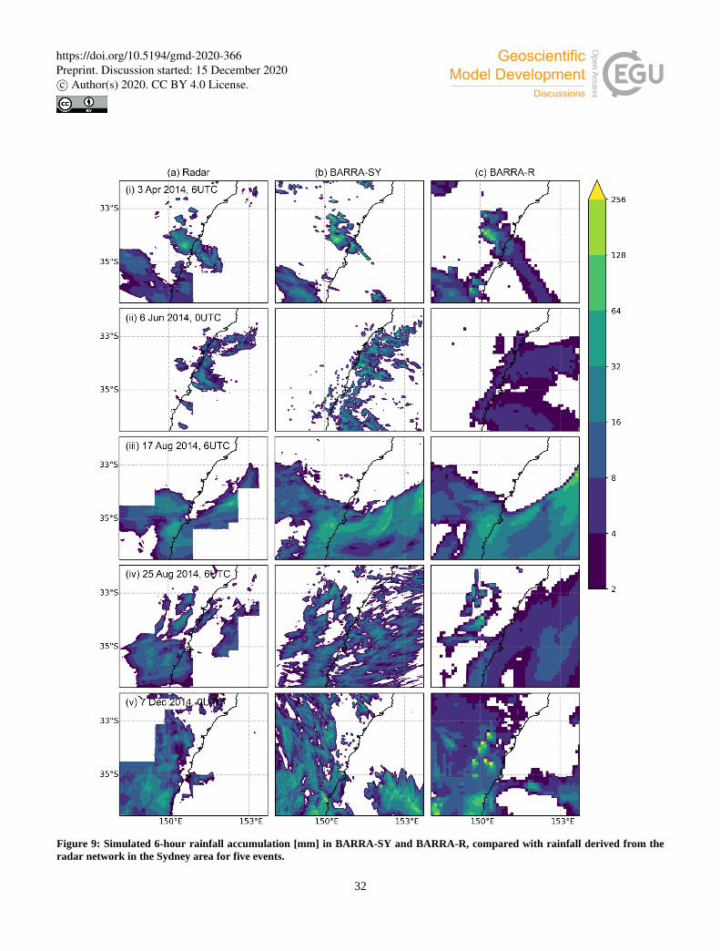
32

Figure 9: Simulated 6-hour rainfall accumulation [mm] in BARRA-SY and BARRA-R, compared with rainfall derived from the

radar network in the Sydney area for five events.


33

755

Figure 10: Aggregated FSS across 1323 6-hour storm events as a function of neighbourhood distance (degrees) for 6h rainfall

above three percentile thresholds (distinguished by colours, percentile values, and observed amount in mm). The solid curves

indicate the score for BARRA-SY, dotted curves for BARRA-R, and the dashed horizontal lines the uniform score (FSSuniform) for

each threshold as specified by Roberts and Lean (2007). All 1323 6-hour events have at observations matching the 59th and 92nd

threshold values, however only 97% of BARRA-SY events matched the 99.9th threshold and only 81% of BARRA-R events. 760

765


34

Table 1: Major differences between BARRA-C, BARRA-R and RAL1-M models. The configurations for BARRA-R are described 770 in Su et al. (2019) and Walters et al. (2017), and those for RAL1-M in Bush et al. (2020).

Aspects BARRA-R BARRA-C RAL1-M

Nesting setup Nested in 6-hourly ERA-

Interim boundary conditions

Nested in hourly BARRA-R

boundary conditions

NA

Horizontal grid length in

radial resolution

0.11⁰ 0.0135⁰ 0.0135 to 0.04⁰

Vertical model level set 70 levels, with 50 levels

below 18 km, and 20 levels

above this, fixed model lid of

80 km above the sea level.

70 levels, with 61 levels below 18 km, 9 levels above this,

fixed model lid of 40 km above sea level

Model timestep 300 seconds 60 seconds 60-100 seconds, depending

on the model resolution

UM model version 10.2 10.6 ≥ 10.6

JULES model version 3.0 4.7 ≥ 4.8

Data assimilation 6-hourly 4D variational

analysis

None NA

Moisture variable SL

advection schemes

Quasi-monotone (Bermejo and Staniforth, 1992) Posteriori monotonicity filter

(PMF)

Convective

parameterization scheme

Mass-flux convection

scheme of Gregory and

Rowntree (1990)

None

Gaseous absorption

(radiation) scheme

GA6 (Walters et al., 2017) GA7 (Walters et al., 2019)

Include spectral land-

surface albedo

No Yes

Canopy radiation back-

scatter scheme

Isotropic Anisotropic

Cloud microphysics

scheme

Single moment scheme

based on Wilson and Ballard

(1999)

Wilson and Ballard (1999), with prognostic graupel

(Wilkinson and Bornemann, 2014) and improved warm rain

scheme (Boutle et al., 2014a)

Boundary layer scheme 1D vertical turbulent mixing

scheme of Lock et al. (2000)

Blended boundary layer parameterisation (Boutle et al.,

2014b)

Land surface and

hydrology

GA6 (Walters et al., 2017), PDM subgrid-scale heterogeneity,

JULES urban parameters are optimized for Australia (Dharssi

et al., 2015)

GA7 (Walters et al., 2019)

where TOPMODEL is used

BL stochastic

perturbations

None Perturbation to temperature Perturbation to temperature

and moisture

BL stability functions For stable BL, the “sharp”

function of Lock et al. (2016)

is used over the sea, and over

land is a blended

combination of the Louis

(1979) and the “sharpest”

function, for heights below

200 m. The convective BL

stability functions are based

on UKMO Large-Eddy

model simulations.

The “sharpest” function for stable BL everywhere. The

convective BL stability functions are based on UKMO Large-

Eddy model simulations.

Critical relative humidity

profile

0.92 in the lowest layer, with

a gradual decrease to 0.8 at

model level 17 (~2100 km).

0.96 in the lowest layer, and decrease to 0.8 at model level 15

(~850 km).


BARRA v1.0: Kilometre-scale downscaling of an Australian ...

Documents

Transcript of BARRA v1.0: Kilometre-scale downscaling of an Australian ...