EFTCAMB/EFTCosmoMC: Numerical Notes v1.0

Bin Hu1, Marco Raveri2,3, Noemi Frusciante2,3, Alessandra Silvestri2,3,41 Institute Lorentz, Leiden University, PO Box 9506, Leiden 2300 RA, The Netherlands

2 SISSA - International School for Advanced Studies, Via Bonomea 265, 34136, Trieste, Italy3 INFN, Sezione di Trieste, Via Valerio 2, I-34127 Trieste, Italy

4 INAF-Osservatorio Astronomico di Trieste, Via G.B. Tiepolo 11, I-34131 Trieste, Italy

EFTCAMB/EFTCosmoMC are publicly available patches to the CAMB/CosmoMC codes imple-menting the effective field theory approach to single scalar field dark energy and modified gravitymodels. With the present numerical notes we provide a guide to the technical details of the code.Moreover we reproduce, as they appear in the code, the complete set of the modified equations andthe expressions for all the other relevant quantities used to construct these patches. We submitthese notes to the arXiv to grant full and permanent access to this material which provides veryuseful guidance to the numerical implementation of the EFT framework. We will update this set ofnotes when relevant modifications to the EFTCAMB/EFTCosmoMC codes will be released.The present version is based on EFTCAMB/EFTCosmoMC May14.

PACS numbers: 98.80

Contents

I. Introduction 1

II. The structure of the code 3

III. The structure of the modification 3A. Structure of the EFTCAMB modification 4B. Structure of the EFTCosmoMC modification 5

IV. Implementation of the modified equations 6A. Background 6B. Linear Perturbations in EFT: code notation 7C. Initial Conditions 11

V. Pure EFT models 11

VI. Mapping EFT models 12A. Designer f(R) 12

References 14

I. INTRODUCTION

In the quest to address one of the most pressing problems of modern cosmology, i.e. cosmic acceleration, an effectivefield theory approach has been recently proposed [1, 2]. The virtue of this approach relies in the model-independentdescription of this phenomenon as well as in the possibility to cast into the EFT language most of the single fieldDE/MG gravity models of cosmological interest [1–4]. The EFT action is written in unitary gauge and Jordanframe and it contains all the operators invariant under time-dependent spatial diffeomorphisms, ordered in power ofperturbations and derivatives. These operators enter in the action with a time dependent function in front of them,to which we will refer to as EFT functions. The DE/MG models encoded in this formalism have one extra scalard.o.f. and a well defined Jordan frame; in unitary gauge the scalar field is hidden in the metric. In order to studythe dynamics of scalar perturbations, it is better to make its dynamics manifest via the Stuckelberg technique, i.e.restoring the time diffeomorphism invariance through an infinitesimal time coordinate transformation. Then a new

arX

iv:1

405.

3590

v1 [

astr

o-ph

.IM

] 1

4 M

ay 2

014

2

scalar field π appears in the action, the so called Stuckelberg field.The EFT action in conformal time reads

S =

∫d4x√−gm2

0

2[1 + Ω(τ + π)]R+ Λ(τ + π)− c(τ + π)a2

[δg00 − 2

π

a2+ 2Hπ

(δg00 − 1

a2− 2

π

a2

)+ 2πδg00

+2g0i∂iπ −π2

a2+ gij∂iπ∂jπ −

(2H2 + H

) π2

a2+ ...

]+M4

2 (τ + π)

2a4

(δg00 − 2

π

a2− 2Hπa2

+ ...

)2

−M31 (τ + π)

2a2

(δg00 − 2

π

a2− 2Hπa2

+ ...

)(δKµ

µ + 3Haπ +∇2π

a2+ ...

)

−M22 (τ + π)

2

(δKµ

µ + 3Haπ +∇2π

a2+ ...

)2

−M23 (τ + π)

2

(δKi

j +Haπδij +

1

a2∇i∇jπ + ...

)(δKj

i +Haπδji +

1

a2∇j∇iπ + ...

)

+M2(τ + π)

2a2

(δg00 − 2

π

a2− 2Ha2π + ...

) (δR(3) + 4

Ha∇2π + ...

)+m2

2(τ + π) (gµν + nµnν) ∂µ(a2g00 − 2π − 2Hπ + ...

)∂ν(a2g00 − 2π − 2Hπ + ...

)+ ...

+ Sm[gµν , χi],

(1)

where m20 is the Planck mass, overdots represent derivatives with respect to conformal time and ∇ indicates three

dimensional spatial derivatives. Ω,Λ,c are the only three EFT functions describing the background dynamics, hencethe name background functions. While the dynamics of linear scalar perturbations is described by the second orderEFT functions, M2, M1, M2, M3, M ,m2, in combination with the background ones. We parametrize the conformalcoupling to gravity via the function 1 + Ω instead of Ω [1, 2] for reasons of numerical accuracy. Finally, Sm is theaction for all matter fields, χi. The EFT approach relies on the assumption of the validity of the weak equivalenceprinciple which ensures the existence of a metric universally coupled to matter fields and therefore of a well definedJordan frame.

In [5, 6], we introduced EFTCAMB which is a patch of the publicly available Einstein-Boltzmann solver,CAMB [7, 8]. The code implements the EFT approach, allowing to study the linear cosmological perturbations in amodel-independent framework via the pure EFT procedure, although it ensures to investigate the dynamics of linearperturbations of specific single scalar field DE/MG models via the mapping EFT procedure, once the matching isworked out. EFTCAMB evolves the full perturbation equations on all linear scales without relying on any quasistatic approximation. Moreover it checks the stability conditions of perturbations in the dark sector in order toensure that the underlying gravitational theory is acceptable. Finally, it enables to choose the expansion historyamong ΛCDM, wCDM and CPL backgrounds, allowing phantom-divide crossings. To interface EFTCAMB withcosmological observations we equipped it with a modified version of CosmoMC [9], what we dub EFTCosmoMC [6].EFTCosmoMC allows to practically perform tests of gravity and get constraints on the parameter space usingcosmological data sets. The stability conditions implemented in EFTCAMB translate into EFTCosmoMC as viabilitypriors to impose on parameters describing the dark sector. The first release of the code includes data such as Planck,WP, BAO and Planck lensing. The EFTCAMB/EFTCosmoMC package is now publicly available for downloadat http://www.lorentz.leidenuniv.nl/~hu/codes/.

Throughout this Numerical Notes we will always use the following conventions:

• The overdot represents derivation with respect to conformal time τ while the prime represents derivation withrespect to the scale factor a, unless otherwise specified.

• In what follows we define a new dimensionless Stuckelberg field: π, i.e. the π-field in the action (1) multipliedby H0 and divided by a. For the rest of the notes we will suppress the tilde to simplify the equations so π iswritten as π, if there is no confusion.

• We redefine all the second order EFT functions to make them dimensionless and to facilitate their inclusion in

3

the code:

α41 =

M42

m20H

20

, α32 =

M31

m20H0

, α23 =

M22

m20

,

α24 =

M23

m20

, α25 =

M2

m20

, α26 =

m22

m20

. (2)

• We define all the EFT functions Ω, c, Λ and the α-functions as function of the scale factor a .

II. THE STRUCTURE OF THE CODE

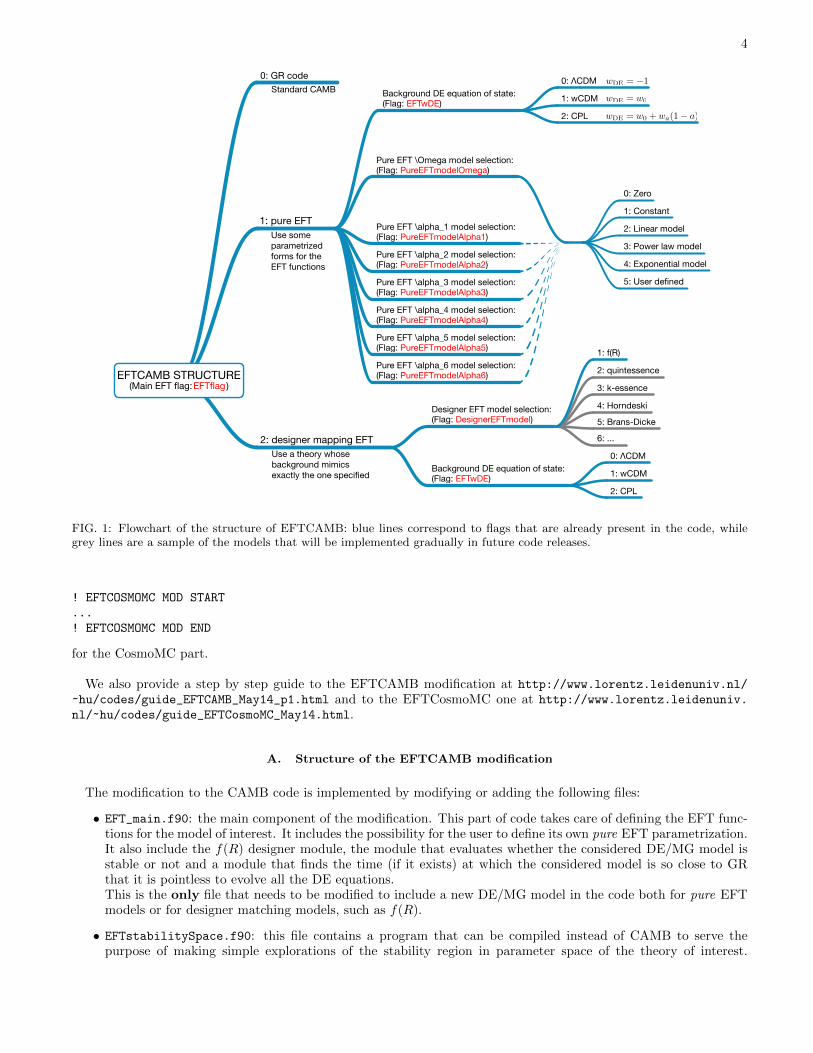
The structure of the EFTCAMB code is illustrated in the flowchart of Figure 1. There is a number associated toeach model selection flag; such number is reported in Figure 1 and it controls the behaviour of the code. The maincode flag is EFTflag which is the starting point after which all the other sub-flags can be chosen according to the userinterests.

• The number EFTflag = 0 corresponds to the standard CAMB code. Every EFT modification to the code isautomatically excluded by this choice.

• The number EFTflag = 1 corresponds to pure EFT models. The user needs then to select a model for thebackground expansion history via the EFTwDE flag. The built-in models for the dark energy equation of stateare: ΛCDM, wCDM and CPL, corresponding respectively to EFTwDE = 0, 1, 2.The ΛCDM model is then fully specified, while for the other two models the user needs to insert a particularvalue for w0 and w0, wa according to the background expansion history that one wants to investigate.The implementation details of the dark energy equations of state can be found in Section IV A. Finally, tofully specify the pure EFT model, one has to fix the EFT functions behaviour as functions of the scale factora. The corresponding flags for the model selection are: PureEFTmodelOmega for the model selection of the EFTfunction Ω(a) and PureEFTmodelAlphai, with i = 1, .., 6 for the αi(a) EFT functions. Some built-in models arealready present in the code and can be selected with the corresponding number, see Flowchart 1. The detailsabout these models can be found in Section V. After setting these flags the user has to define the values of theEFT model parameters for the chosen model. Every other value of parameter and flag which do not concernthe chosen model is automatically ignored.

• The number EFTflag = 2 corresponds to the mapping EFT procedure. Also in this case the EFTwDE flag controlsthe background expansion history which works as in the previous case.For the mapping case the user can investigate a particular DE/MG model once the matching with the EFTfunctions is provided and the background evolution has been implemented in the EFT code.The model selection flag for the mapping EFT procedure is DesignerEFTmodel. The first code release has onebuilt-in model, namely designer f(R) theories which corresponds to DesignerEFTmodel = 1. The implementa-tion details of such model are presented in Section VI A.Models corresponding to the grey lines in the flowchart 1 are some of the models that can be cast into the EFTformalism and that will be gradually implemented in future code releases.

III. THE STRUCTURE OF THE MODIFICATION

In order to implement the EFT formalism in the CAMB and CosmoMC codes we had to modify several files. Welist them in this section to help the user keep track of what the EFT code is doing and how.To further help the user in understanding our part of code and/or applying the EFT modification to an alreadymodified version of CAMB/CosmoMC we enclosed every modification that we made inside the following commentedcode lines:

! EFTCAMB MOD START...! EFTCAMB MOD END

for the CAMB part and:

4

FIG. 1: Flowchart of the structure of EFTCAMB: blue lines correspond to flags that are already present in the code, whilegrey lines are a sample of the models that will be implemented gradually in future code releases.

! EFTCOSMOMC MOD START...! EFTCOSMOMC MOD END

for the CosmoMC part.

We also provide a step by step guide to the EFTCAMB modification at http://www.lorentz.leidenuniv.nl/

~hu/codes/guide_EFTCAMB_May14_p1.html and to the EFTCosmoMC one at http://www.lorentz.leidenuniv.nl/~hu/codes/guide_EFTCosmoMC_May14.html.

A. Structure of the EFTCAMB modification

The modification to the CAMB code is implemented by modifying or adding the following files:

• EFT_main.f90: the main component of the modification. This part of code takes care of defining the EFT func-tions for the model of interest. It includes the possibility for the user to define its own pure EFT parametrization.It also include the f(R) designer module, the module that evaluates whether the considered DE/MG model isstable or not and a module that finds the time (if it exists) at which the considered model is so close to GRthat it is pointless to evolve all the DE equations.This is the only file that needs to be modified to include a new DE/MG model in the code both for pure EFTmodels or for designer matching models, such as f(R).

• EFTstabilitySpace.f90: this file contains a program that can be compiled instead of CAMB to serve thepurpose of making simple explorations of the stability region in parameter space of the theory of interest.

5

This proves extremely helpful to understand and visualise the shape of the parameter space of a theory beforeexploring it with CosmoMC. For a direct application of this see Figure (1) in [6].

• equations_EFT.f90: this is a modified version of the standard CAMB equations file. It contains all theequations that the code needs to solve to get the full behaviour of perturbations in DE/MG models. Theseequations are reported in Section IV and being written in terms of the EFT functions there is no need for theuser to modify this file to include new DE/MG models in CAMB.

• cmbmain.f90: it includes modification of the standard CAMB file to run the designer code, the stability checkand the return to GR detection just after EFTCAMB is launched. It also contains an optional code that willprint the behaviour of perturbations in the DE/MG model that is considered. The latter part of code is notcontrolled by the parameter file so the user has to search for it in the code and manually activate it. It is alsopossible to use it at debug purposes.

• inidriver.F90: it contains a small modification of the CAMB file to read EFT parameters from the params.inifile.

• modules.f90: it is a modified version of the standard CAMB file to include EFT parameters within the standardcosmological parameters.

• params.ini: this file allows to choose the input values for the EFT model parameters and the model selectionflags.

• Makefile_main: it is a modified version of the standard file to compile the code using all the relevant EFT files.Inside here there is the option to compile the EFTstabilitySpace program.

B. Structure of the EFTCosmoMC modification

To interface CosmoMC with EFTCAMB we had to modify the following files:

• params_CMB_EFT.ini: to specify the EFT model parameters that are sampled in the MCMC run and theirpriors.

• common_batch1_EFT.ini: to read cosmological parameters from params_CMB_EFT.ini.

• EFT_params.ini: to let the user choose the model via the selection flags.

• params_CMB.paramnames: to add the names of the EFT model parameters.

• calclike.f90: to perform the stability check on the considered model for the specific choice of cosmologicalparameters that are being considered by the MCMC sampler and reject them if the theory is found to beunstable.

• CMB_Cls_simple.f90: to pass the EFT model parameters and the values of the model selection flags to EFT-CAMB.

• cmbtypes.f90: to add the EFT model parameters into the set of CosmoMC parameters and store the values ofthe model selection flags in cmbtypes.

• driver.F90: to read the values of the model selection flags from the parameters files.

• Makefile: to compile the whole program with the EFTCAMB/EFTCosmoMC files.

• params_CMB.f90: to increase the number of CosmoMC parameters and associate the EFT parameter name tothe one in the parameters files.

• settings.f90: to increase the number of theory parameters.

As of now the EFTCosmoMC May14 code does not enforce automatically the compatibility between the modelselection flags and the parameters that are included in the MCMC run. This means that the user has to do thefollowing to properly launch a run:

• At first the proper values for the EFT model selection flags have to be chosen in the file EFT_params.iniaccording to the scheme in Figure 1.

6

• Then the user has to modify params_CMB_EFT.ini to select the parameters to include in the run, their centervalues and priors.In order to exclude unwanted EFT parameters from the run, their start width and propose width have tobe set to zero while for the parameters related to the previously selected model these two have to be chosendifferent from zero.Since EFTCAMB enforces viability priors it is then sufficient that the standard CosmoMC priors are set to avalue that reasonably includes the stable region in parameter space.We then suggest to set the center of a parameter relatively far from its GR limit as the parameter space of agiven model might be not well behaved in the vicinity of that point.

• After these two steps the run can be launched in the standard way.

IV. IMPLEMENTATION OF THE MODIFIED EQUATIONS

The implementation of the background in the code is described at length in [5]. Here we shall review some of themore technical aspects and reproduce the equations in the form in which they enter the code.

A. Background

Given the high degree of freedom already at the level of background, and since the focus will be on the dynamicsof linear perturbations, it is common to adopt a designer approach as described in [1, 2]. First of all one writes thebackground equations as follows:

H2 =8πG

3a2(ρm + ρDE) ,

H = −4πG

3a2 (ρm + ρDE + 3Pm + 3PDE) = −H

2

2− 8πGa2Ptot

2,

H = 8πGa2ρmH(

1

6+ wm +

3

2w2m

)+ 8πGa2ρDEH

(1

6+ wDE +

3

2w2

DE −1

2aw′DE

), (3)

where the prime stands for derivative w.r.t. the scale factor a, ρm, Pm are the energy density and pressure of matter(e.g. dark matter, radiation and massless neutrinos) and ρDE, PDE encode the contributions from the extra scalarfield into the form of an energy density and pressure of dark energy. One has the following continuity equations, andcorresponding solutions:

ρm + 3H (ρm + Pm) = 0 , ρm =3H2

0

8πGΩ0m a−3(1+wm) ,

ρDE + 3HρDE [1 + wDE(a)] = 0 , ρDE =3H2

0

8πGΩ0

DE exp

[− 3

∫ a

1

(1 + wDE(a))

ada

], (4)

where Ω0m,DE is the energy density parameter today, respectively of matter sector and dark energy, and H0 is the

present time Hubble parameter.With this setup, a background is fixed via the specification of wDE. We consider three different models in the code:

- The ΛCDM expansion history: wDE = −1 and ρDE = m20Λ;

- The wCDM model: wDE = const 6= −1 and ρDE = 3m20H

20 Ω0

DEa−3(1+wDE);

- The CPL parametrization [10, 11]: wDE(a) = w0 + wa(1− a) and

ρDE = 3m20H

20 Ω0

DEa−3(1+w0+wa) exp (−3wa(1− a)) ,

where w0 and wa are constant and indicate, respectively, the value and the derivative of wDE today.

One can then determine c,Λ in terms of the expansion history and Ω(a); namely, combining eq. (3) and eq. (4) withthe EFT background eqs. (12,13) in [5] one has:

ca2

m20

=(H2 − H

)(Ω +

aΩ′

2

)− a2H2

2Ω′′ +

1

2

a2ρDE

m20

(1 + wDE) , [Mpc−2] (5)

7

Λa2

m20

=− Ω(

2H+H2)− aΩ′

(2H2 + H

)− a2H2Ω′′ + wDE

a2ρDE

m20

, [Mpc−2] (6)

ca2

m20

=H2

(−3 (1 + wDE)

2+ aw′DE

) ρDEa2

m20

− Ω(H − 4HH+ 2H3

)+aΩ′

2

(−H+HH+H3

)+

1

2a2HΩ′′

(H2 − 3H

)− 1

2a3H3Ω′′′ , [Mpc−3] (7)

Λa2

m20

=− 2Ω(H − HH −H3

)− a2Ω′′H

(2H2 + 3H

)− a3H3Ω′′′

− aΩ′(

4HH+ H)

+ρDEa

2

m20

H[aw′DE − 3wDE(1 + wDE)

]. [Mpc−3] (8)

As discussed in the Sections V and VI, depending on whether one wants to implement a pure or mapping EFTmodel, the choice for Ω changes. After fixing the expansion history, in the former case one selects an ansatz for Ω(a),while in the latter case one determines via the matching the Ω(a) corresponding to the chosen model. In this caseone has to separately solve the background equations for the given model, which might be done with a model-specificdesigner approach. In fact, this is the methodology we adopt for f(R) models (see Section VI A).

Finally, for the purposes of the code, it is useful to compute the following EFT dark fluid components that can bederived from eq. (10) of [5]:

ρQa2

m20

=2ca2

m20

− Λa2

m20

− 3aH2Ω′ , [Mpc−2] (9)

PQa2

m20

=Λa2

m20

+ a2H2Ω′′ + aHΩ′ + 2aH2Ω′ , [Mpc−2] (10)

ρQa2

m20

=− 3H(ρQa

2

m20

+PQa

2

m20

)+ 3aH3Ω′ , [Mpc−3] (11)

PQa2

m20

=Λa2

m20

+ a3H3Ω′′′ + 3a2HHΩ′′ + aΩ′H+ 3aHHΩ′ + 2a2H3Ω′′ − 2aH3Ω′ . [Mpc−3] (12)

B. Linear Perturbations in EFT: code notation

In this section we write the relevant equations that EFTCAMB uses [12]. We write them in a compact notationthat almost preserves the form of the standard equations simplifying both the comparison with the GR limit and theimplementation in the code.The dynamical equations that EFTCAMB evolves can be written1 as:

A(τ) π +B(τ) π + C(τ)π + k2D(τ)π +H0E(τ) = 0 , (13)

kη =1

1 + Ω

a2(ρm + Pm)

m20

vm2

+k2

3H0F (τ) , (14)

while constraint equations take the form:

σ =1

X(τ)

[ZU(τ) +

1

1 + Ω

3

2k2

a2(ρm + Pm)

m20

vm +F (τ)

H0

], (15)

σ =1

X(τ)

[−2H [1 + V (τ)]σ + kη − 1

k

a2P

m20

Π

1 + Ω+N(τ)

H0

], (16)

σ =1

X(τ)

[−2 (1 + V )

(Hσ +Hσ

)− 2HσV + kη +

1

k

aHΩ′

(1 + Ω)2

a2P

m20

Π− 1

k(1 + Ω)

d

dτ

(a2P

m20

Π

)− Xσ +

N

H0

], (17)

1 Notice that working in the Jordan frame ensures that the energy-momentum conservation equations are not changed with respect totheir GR form. For this reason the evolution equations for density and velocity are not reported here.

8

Z =1

G(τ)

[kη

H+

1

2H(1 + Ω)k

a2δρmm2

0

+L(τ)

kH0

], (18)

Z =1

U(τ)

[−2H [1 + Y (τ)]Z + kη − 1

1 + Ω

3

2k

a2δPmm2

0

− 3

2k(1 + Ω)

M(τ)

H0

],

=1

U(τ)

[−2HZ

(1 + Y − G

2

)− 1

2(1 + Ω)k

a2δρmm2

0

− 3

2(1 + Ω)k

a2δPmm2

0

− HLH0k

− 3

2(1 + Ω)k

M

H0

], (19)

where 2kZ ≡ h and 2kσ∗ ≡ h+6η are the standard CAMB variables. In these expressions we wrote the same prefactor,X, in (15) and (16), and U , in (15) and (19), but we have to stress that they might be different if other second orderEFT operators are considered. In addition the last expression (19) has two forms: the first is the standard one whilethe second one is used when the CAMB code uses the RSA approximation.At last, to compute the observable spectra we had to define two auxiliary quantities:

EFTISW = σ + kη =1

X

[− 2 [1 + V ]

(Hσ +Hσ

)− 2HσV +

(1 +X)

2(1 + Ω)

a2(ρm + Pm)

m20

vm

+1

k

aHΩ′

(1 + Ω)2

a2P

m20

Π− 1

k(1 + Ω)

d

dτ

(a2P

m20

Π

)+

(1 +X)k2

3H0F − Xσ +

N

H0

], (20)

EFTLensing = σ + kη =1

X

[−2H (1 + V )σ + (1 +X)kη − 1

k(1 + Ω)

a2P

m20

Π +N(τ)

H0

]. (21)

The coefficients for the π field equation, once a complete de-mixing is achieved, can not be divided into contributionsdue to one operator at a time so we write here their full form:

A =ca2

m20

+ 2a2H20α

41 +

3

2a2

(HΩ′ +H0α

32

)22(1 + Ω) + α2

3 + α24

+ 4a2α26k

2 , (22)

B =ca2

m20

+ 4Hca2

m20

+ 8a2HH0

(α4

1 + aα31α′1

)+ 4a2k2H

(3α2

6 + aα6α′6

)+ ak2 α2

4 + 2α25

2(1 + Ω)− 2α24

(HΩ′ +H0α

32

)− a HΩ′ +H0α

32

4(1 + Ω) + 6α23 + 2α2

4

[− 3

a2(ρq + PQ)

m20

− 3aH2Ω′

(4 +

HH2

+ aΩ′′

Ω′

)− 3aHH0

(4α3

2 + 3aα22α′2

)−(9α2

3 − 3α24

) (H − H2

)+ k2

(3α2

3 − α24 + 4α2

5

) ]+

1

1 + Ω + 2α25

(aHΩ′ + 2H

(α2

5 + 2α5α′5

)− (1 + Ω)

aHΩ′ + aH0α32

2(1 + Ω) + 3α23 + α2

4

)·

·[−a

2c

m20

+3

2aH2Ω′ − 2a2H0α

41 − 4α2

6k2 +

3

2aHH0α

32

], (23)

C = +H ca2

m20

+(

6H2 − 2H) ca2

m20

+3

2aHΩ′

(H − 2H3

)+ 6H2H2

0α41a

2 + 2a2HH20α

41 + 8a3H2H2

0α31α′1

+3

2

(H − H2

)2 (α2

4 + 3α23

)+

9

2HH0a

(H − H2

) (α3

2 + aα22α′2

)+a

2H0α

32

(3H − 12HH+ 6H3

)− a HΩ′ +H0α

32

4(1 + Ω) + 6α23 + 2α2

4

[− 3

a2PQm2

0

− 3H(a2ρQm2

0

+a2PQm2

0

)− 3aH3

(aΩ′′ + 6Ω′ + 2

HH2

Ω′

)+ 3

(H − 2HH

) (α2

4 + 3α23

)+ 6H

(H − H2

) (3α2

3 + 3aα3α′3 + α2

4 + aα4α′4

)− 3aH0

(3H2α3

2 + Hα32 + 3aH2α2

2α′2

)]+

1

1 + Ω + 2α25

(aHΩ′ + 2H

(α2

5 + 2aα5α′5

)− (1 + Ω)

aHΩ′ + aH0α32

2(1 + Ω) + 3α23 + α2

4

)·

·[− 1

2

a2ρQm2

0

−Ha2c

m20

+3

2aHΩ′

(3H2 − H

)− 2a2HH2

0α41 −

3

2aH0α

32

(H − 2H2

)− 3H

(H − H2

)(3

2α2

3 + α24

)],

9

D =ca2

m20

− 1

2aHH0

(α3

2 + 3aα22α′2

)+(H2 − H

) (3α2

3 + α24

)+ 4a2

(Hα2

6 + 2H2α26 + aH2α6α

′6

)+ 2

(Hα2

5 + 2aH2α5α′5

)− a HΩ′ +H0α

32

4(1 + Ω) + 6α23 + 2α2

4

[− 2aHΩ′ + 4Hα2

5 − 2H(3α2

3 + 3aα3α′3 + α2

4 + aα4α′4

) ]+

1

1 + Ω + 2α25

(aHΩ′ + 2H

(α2

5 + 2aα5α′5

)− (1 + Ω)

aHΩ′ + aH0α32

2(1 + Ω) + 3α23 + α2

4

)·

·[

1

2aHΩ′ − 2Hα2

5 +1

2aH0α

32 +

3

2Hα2

3 −Hα24 − 4Hα2

6

]+

α24 + 2α2

5

2(1 + Ω)− 2α24

[a2 (ρQ + PQ)

m20

+ aH2Ω′ − α24

(H − H2

)+ aHH0α

32 + 3α2

3

(H2 − H

)]+ k2

[α2

3

2+α2

4

2+

α24 + 2α2

5

2(1 + Ω)− 2α24

(α2

3 + α24

) ],

E =

ca2

m20

− 3

2aH2Ω′ − 1

2aHH0

(2α3

2 + 3aα22α′2

)+

1

2α2

3

(k2 − 3H+H2

)+

1

2α2

4

(k2 − H+H2

)− a HΩ′ +H0α

32

4(1 + Ω) + 6α23 + 2α2

4

[− 2H (aΩ′ + 2(1 + Ω))− 2H

(3α2

3 + 3aα3α′3 + α2

4 + aα4α′4

) ]+

1

1 + Ω + 2α25

(aHΩ′ + 2H

(α2

5 + 2aα5α′5

)− (1 + Ω)

aHΩ′ + aH0α32

2(1 + Ω) + 3α23 + α2

4

)·

·[H(

1 + Ω +aΩ′

2

)+

1

2aH0α

32 +

3

2Hα2

3 +Hα24

]+

α24 + 2α2

5

2(1 + Ω)− 2α24

k2(α2

4 + α23

)kZ

+ 3aHΩ′ +H0α

32

4(1 + Ω) + 6α23 + 2α2

4

(a2δPm

m20

)+

α24 + 2α2

5

2(1 + Ω)− 2α24

k

(a2 (ρ+ P ) vm

m20

)− 1

2

1

1 + Ω + 2α25

(aHΩ′ + 2H

(α2

5 + 2aα5α′5

)− (1 + Ω)

aHΩ′ + aH0α32

2(1 + Ω) + 3α23 + α2

4

)(a2δρm

m20

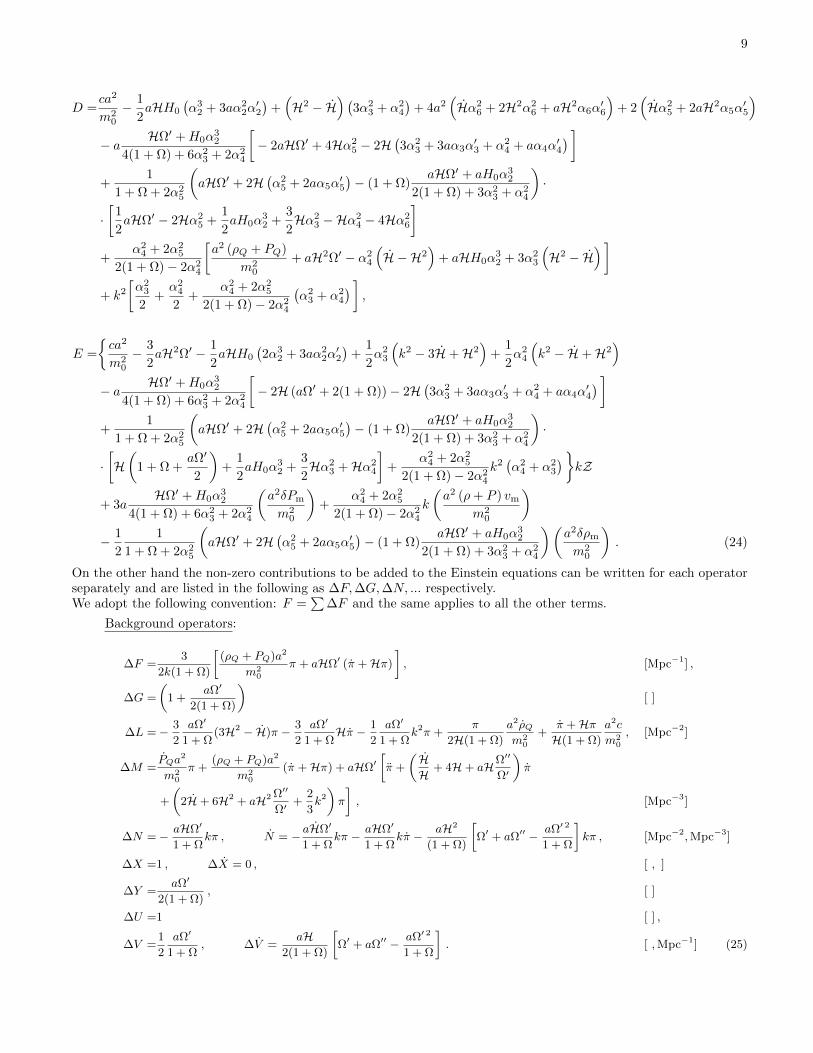
). (24)

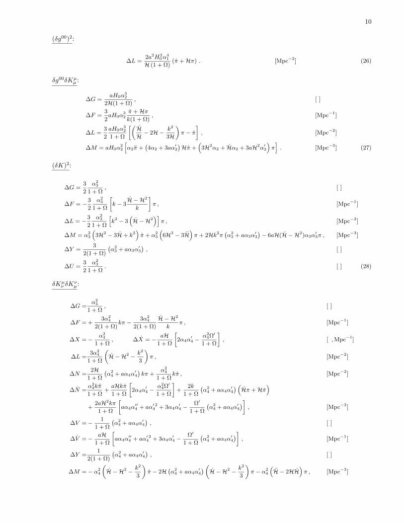
On the other hand the non-zero contributions to be added to the Einstein equations can be written for each operatorseparately and are listed in the following as ∆F,∆G,∆N, ... respectively.We adopt the following convention: F =

∑∆F and the same applies to all the other terms.

Background operators:

∆F =3

2k(1 + Ω)

[(ρQ + PQ)a2

m20

π + aHΩ′ (π +Hπ)

], [Mpc−1] ,

∆G =

(1 +

aΩ′

2(1 + Ω)

)[ ]

∆L =− 3

2

aΩ′

1 + Ω(3H2 − H)π − 3

2

aΩ′

1 + ΩHπ − 1

2

aΩ′

1 + Ωk2π +

π

2H(1 + Ω)

a2ρQm2

0

+π +HπH(1 + Ω)

a2c

m20

, [Mpc−2]

∆M =PQa

2

m20

π +(ρQ + PQ)a2

m20

(π +Hπ) + aHΩ′[π +

(HH + 4H+ aHΩ′′

Ω′

)π

+

(2H+ 6H2 + aH2 Ω′′

Ω′+

2

3k2)π

], [Mpc−3]

∆N =− aHΩ′

1 + Ωkπ , N = −aHΩ′

1 + Ωkπ − aHΩ′

1 + Ωkπ − aH2

(1 + Ω)

[Ω′ + aΩ′′ − aΩ′ 2

1 + Ω

]kπ , [Mpc−2,Mpc−3]

∆X =1 , ∆X = 0 , [ , ]

∆Y =aΩ′

2(1 + Ω), [ ]

∆U =1 [ ] ,

∆V =1

2

aΩ′

1 + Ω, ∆V =

aH2(1 + Ω)

[Ω′ + aΩ′′ − aΩ′ 2

1 + Ω

]. [ ,Mpc−1] (25)

10

(δg00)2:

∆L =2a2H2

0α41

H (1 + Ω)(π +Hπ) . [Mpc−2] (26)

δg00δKµµ :

∆G =aH0α

32

2H(1 + Ω), [ ]

∆F =3

2aH0α

32π +Hπk(1 + Ω)

, [Mpc−1]

∆L =3

2

aH0α32

1 + Ω

[(HH − 2H− k2

3H

)π − π

], [Mpc−2]

∆M = aH0α22

[α2π +

(4α2 + 3aα′2

)Hπ +

(3H2α2 + Hα2 + 3aH2α′2

)π]. [Mpc−3] (27)

(δK)2:

∆G =3

2

α23

1 + Ω, [ ]

∆F = −3

2

α23

1 + Ω

[k − 3

H − H2

k

]π , [Mpc−1]

∆L = −3

2

α23

1 + Ω

[k2 − 3

(H − H2

)]π , [Mpc−2]

∆M = α23

(3H2 − 3H+ k2

)π + α2

3

(6H3 − 3H

)π + 2Hk2π

(α23 + aα3α

′3

)− 6aH(H − H2)α3α

′3π , [Mpc−3]

∆Y =3

2(1 + Ω)

(α23 + aα3α

′3

), [ ]

∆U =3

2

α23

1 + Ω. [ ] (28)

δKµν δK

νµ:

∆G =α24

1 + Ω, [ ]

∆F = +3α2

4

2(1 + Ω)kπ − 3α2

4

2(1 + Ω)

H − H2

kπ , [Mpc−1]

∆X =− α24

1 + Ω, ∆X = − aH

1 + Ω

[2α4α

′4 −

α24Ω′

1 + Ω

], [ ,Mpc−1]

∆L =3α2

4

1 + Ω

(H − H2 − k2

3

)π , [Mpc−2]

∆N =2H

1 + Ω

(α24 + aα4α

′4

)kπ +

α24

1 + Ωkπ , [Mpc−2]

∆N =α24kπ

1 + Ω+aHkπ1 + Ω

[2α4α

′4 −

α24Ω′

1 + Ω

]+

2k

1 + Ω

(α24 + aα4α

′4

) (Hπ +Hπ

)+

2aH2kπ

1 + Ω

[aα4α

′′4 + aα′ 24 + 3α4α

′4 −

Ω′

1 + Ω

(α24 + aα4α

′4

)], [Mpc−3]

∆V =− 1

1 + Ω

(α24 + aα4α

′4

), [ ]

∆V =− aH1 + Ω

[aα4α

′′4 + aα′ 24 + 3α4α

′4 −

Ω′

1 + Ω

(α24 + aα4α

′4

)], [Mpc−1]

∆Y =1

2(1 + Ω)

(α24 + aα4α

′4

), [ ]

∆M =− α24

(H − H2 − k2

3

)π − 2H

(α24 + aα4α

′4

)(H − H2 − k2

3

)π − α2

4

(H − 2HH

)π , [Mpc−3]

11

∆U =α24

2(1 + Ω). [ ] (29)

δg00δR(3):

∆M = −4α25k

2

3(π +Hπ) , [Mpc−3]

∆N =2α2

5k

1 + Ω(π +Hπ) , [Mpc−2]

∆N =2α2

5k

1 + Ω

(π +Hπ + Hπ

)+

2akH1 + Ω

(π +Hπ)

[2α5α

′5 −

α25Ω′

1 + Ω

]. [Mpc−3] (30)

(gµν + nµnν)∂µδg00∂νδg

00:

∆L =4α2

6k2

H(1 + Ω)(π +Hπ) . [Mpc−2] (31)

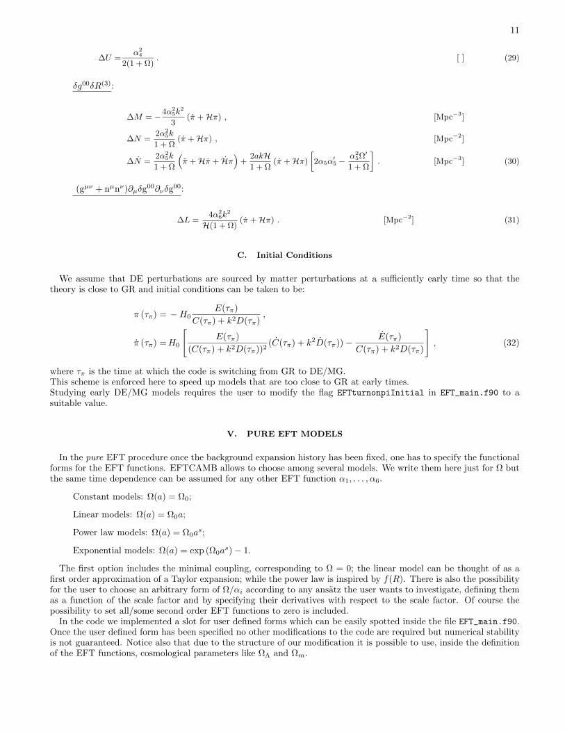
C. Initial Conditions

We assume that DE perturbations are sourced by matter perturbations at a sufficiently early time so that thetheory is close to GR and initial conditions can be taken to be:

π (τπ) = −H0E(τπ)

C(τπ) + k2D(τπ),

π (τπ) =H0

[E(τπ)

(C(τπ) + k2D(τπ))2(C(τπ) + k2D(τπ))− E(τπ)

C(τπ) + k2D(τπ)

], (32)

where τπ is the time at which the code is switching from GR to DE/MG.This scheme is enforced here to speed up models that are too close to GR at early times.Studying early DE/MG models requires the user to modify the flag EFTturnonpiInitial in EFT_main.f90 to asuitable value.

V. PURE EFT MODELS

In the pure EFT procedure once the background expansion history has been fixed, one has to specify the functionalforms for the EFT functions. EFTCAMB allows to choose among several models. We write them here just for Ω butthe same time dependence can be assumed for any other EFT function α1, . . . , α6.

Constant models: Ω(a) = Ω0;

Linear models: Ω(a) = Ω0a;

Power law models: Ω(a) = Ω0as;

Exponential models: Ω(a) = exp (Ω0as)− 1.

The first option includes the minimal coupling, corresponding to Ω = 0; the linear model can be thought of as afirst order approximation of a Taylor expansion; while the power law is inspired by f(R). There is also the possibilityfor the user to choose an arbitrary form of Ω/αi according to any ansatz the user wants to investigate, defining themas a function of the scale factor and by specifying their derivatives with respect to the scale factor. Of course thepossibility to set all/some second order EFT functions to zero is included.

In the code we implemented a slot for user defined forms which can be easily spotted inside the file EFT_main.f90.Once the user defined form has been specified no other modifications to the code are required but numerical stabilityis not guaranteed. Notice also that due to the structure of our modification it is possible to use, inside the definitionof the EFT functions, cosmological parameters like ΩΛ and Ωm.

12

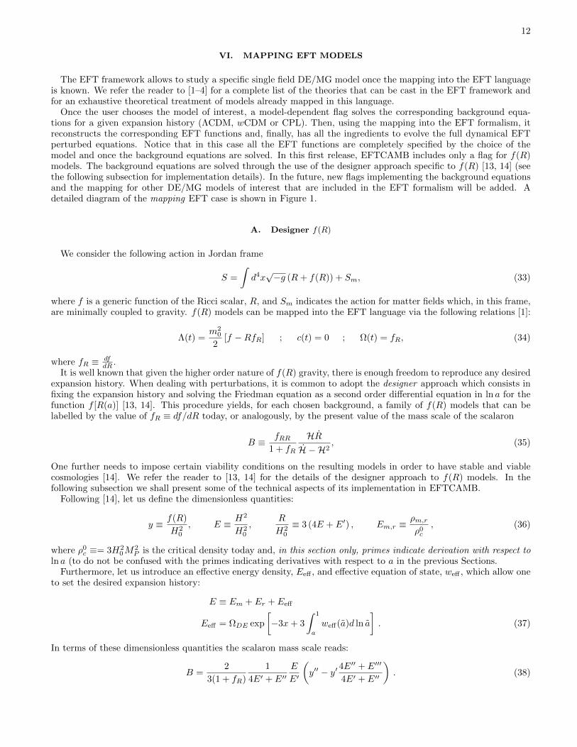
VI. MAPPING EFT MODELS

The EFT framework allows to study a specific single field DE/MG model once the mapping into the EFT languageis known. We refer the reader to [1–4] for a complete list of the theories that can be cast in the EFT framework andfor an exhaustive theoretical treatment of models already mapped in this language.

Once the user chooses the model of interest, a model-dependent flag solves the corresponding background equa-tions for a given expansion history (ΛCDM, wCDM or CPL). Then, using the mapping into the EFT formalism, itreconstructs the corresponding EFT functions and, finally, has all the ingredients to evolve the full dynamical EFTperturbed equations. Notice that in this case all the EFT functions are completely specified by the choice of themodel and once the background equations are solved. In this first release, EFTCAMB includes only a flag for f(R)models. The background equations are solved through the use of the designer approach specific to f(R) [13, 14] (seethe following subsection for implementation details). In the future, new flags implementing the background equationsand the mapping for other DE/MG models of interest that are included in the EFT formalism will be added. Adetailed diagram of the mapping EFT case is shown in Figure 1.

A. Designer f(R)

We consider the following action in Jordan frame

S =

∫d4x√−g (R+ f(R)) + Sm, (33)

where f is a generic function of the Ricci scalar, R, and Sm indicates the action for matter fields which, in this frame,are minimally coupled to gravity. f(R) models can be mapped into the EFT language via the following relations [1]:

Λ(t) =m2

0

2[f −RfR] ; c(t) = 0 ; Ω(t) = fR, (34)

where fR ≡ dfdR .

It is well known that given the higher order nature of f(R) gravity, there is enough freedom to reproduce any desiredexpansion history. When dealing with perturbations, it is common to adopt the designer approach which consists infixing the expansion history and solving the Friedman equation as a second order differential equation in ln a for thefunction f [R(a)] [13, 14]. This procedure yields, for each chosen background, a family of f(R) models that can belabelled by the value of fR ≡ df/dR today, or analogously, by the present value of the mass scale of the scalaron

B ≡ fRR1 + fR

HRH − H2

, (35)

One further needs to impose certain viability conditions on the resulting models in order to have stable and viablecosmologies [14]. We refer the reader to [13, 14] for the details of the designer approach to f(R) models. In thefollowing subsection we shall present some of the technical aspects of its implementation in EFTCAMB.

Following [14], let us define the dimensionless quantities:

y ≡ f(R)

H20

, E ≡ H2

H20

,R

H20

≡ 3 (4E + E′) , Em,r ≡ρm,rρ0c

, (36)

where ρ0c ≡= 3H2

0M2P is the critical density today and, in this section only, primes indicate derivation with respect to

ln a (to do not be confused with the primes indicating derivatives with respect to a in the previous Sections.Furthermore, let us introduce an effective energy density, Eeff , and effective equation of state, weff , which allow one

to set the desired expansion history:

E ≡ Em + Er + Eeff

Eeff = ΩDE exp

[−3x+ 3

∫ 1

a

weff(a)d ln a

]. (37)

In terms of these dimensionless quantities the scalaron mass scale reads:

B =2

3(1 + fR)

1

4E′ + E′′E

E′

(y′′ − y′ 4E

′′ + E′′′

4E′ + E′′

). (38)

13

In EFTCAMB we consider three different background evolutions, namely:

ΛCDM ⇒ Eeff = ΩΛ , weff = −1 ;

wCDM ⇒ Eeff = ΩΛ exp (−3x(1 + w0)) , weff = w0 ;

CPL ⇒ Eeff = ΩΛ exp (−3x(1 + w0)− 3wa (x+ 1− ex)) , weff = w0 + wa(1− a) , (39)

where we have introduced the variable x ≡ ln a.The designer approach will then consist in choosing one of the three expansion histories in (39) and solving the

following equation for y(x)

y′′ −(

1 +E′

2E+R′′

R′

)y′ +

R′

6H20E

y = − R′

H20E

Eeff , (40)

with appropriate boundary conditions that allow us to select the growing mode, as described in [14]. The outcomewill be a family of models labelled by the present day value, B0, of (38). In order to implement eq. (40) in the codewe need to define the following quantities:

g(x) =(1 + w0)x+ wa (x+ 1− ex) ,

g′(x) =(1 + w0) + wa (1− ex) ,

g′′(x) =− wa ex ,g(3)(x) =g′′(x) , (41)

which allow us to rewrite E(x) and its derivatives as follows:

E′ =− 3Ωme−3x − 4Ωre

−4x − 3ΩΛe−3g(x)g′(x) ,

E′′ =9Ωme−3x + 16Ωre

−4x − 3ΩΛe−3g(x)

(g′′(x)− 3g′(x)2

),

E′′′ =− 27Ωme−3x − 64Ωre

−4x − 3ΩΛe−3g(x)

(g(3)(x)− 9g′(x)g′′(x) + 9g′(x)3

). (42)

Once we have solved the background according to the above procedure, there remains only to map the solution intothe EFT language. To this extent we have:

Ω(a) ≡ fR(a) =y′

3(4E′ + E′′). (43)

For the code purposes we need also the derivatives of this function with respect to a, and it turns useful to input theiranalytical expressions directly in the code, rather than having the code evaluate them numerically. We have:

dΩ

da=e−x (−E′′(6Eeff + y) + E′ (y′ − 4(6Eeff + y)) + 2Ey′)

6E (E′′ + 4E′),

d2Ω

da2=e−2x (E′ (E′ (24Eeff − y′ + 4y)− 6E (8E′eff + y′)) + E′′ (E′(6Eeff + y)− 12EE′eff))

12E2 (E′′ + 4E′),

d3Ω

da3=

e−3x

24E3 (E′′ + 4E′)

[2E(E′′ 2(6Eeff + y) + 4E′ 2 (18E′eff + 6Eeff + 2y′ + y) + E′E′′ (18E′eff + 30Eeff − y′ + 5y)

),

+ 12E2 (E′′ (−2E′′eff + 4E′eff − y′) + E′ (−8E′′eff + 16E′eff + y′)) + 3E′ 2 (E′ (y′ − 4(6Eeff + y))− E′′(6Eeff + y))

].

(44)

At this point, having H(a) and Ω(a) at hand, one can go back to the general treatment of the background in theEFT formalism (setting wDE = weff), and use the designer EFT described in Section IV A to determine c and Λ.However, for a matter of numerical accuracy, it is better to determine these functions via the mapping too. We have:

ca2

m20

=0,ca2

m20

= 0 ,

Λa2

m20

=a2H20

2[y − 3fR (4E + E′)] ,

Λa2

m20

= −3

2H2

0H[a3 dΩ

da(4E + E′)

]. (45)

14

[1] G. Gubitosi, F. Piazza and F. Vernizzi, JCAP 1302, 032 (2013), [arXiv:1210.0201 [hep-th]].

[2] J. K. Bloomfield, E. E. Flanagan, M. Park and S. Watson, JCAP 1308, 010 (2013), [arXiv:1211.7054 [astro-ph.CO]].[3] J. Gleyzes, D. Langlois, F. Piazza and F. Vernizzi, JCAP 1308, 025 (2013), [arXiv:1304.4840 [hep-th]].[4] J. Bloomfield, arXiv:1304.6712 [astro-ph.CO].[5] B. Hu, M. Raveri, N. Frusciante and A. Silvestri, arXiv:1312.5742 [astro-ph.CO].[6] M. Raveri, B. Hu, N. Frusciante and A. Silvestri, arXiv:1405.1022 [astro-ph.CO].[7] http://camb.info .[8] A. Lewis, A. Challinor and A. Lasenby, Astrophys. J. 538, 473 (2000), [astro-ph/9911177].[9] A. Lewis and S. Bridle, Phys. Rev. D 66, 103511 (2002) [astro-ph/0205436].

[10] M. Chevallier and D. Polarski, Int. J. Mod. Phys. D 10, 213 (2001), [gr-qc/0009008].[11] E. V. Linder, Phys. Rev. Lett. 90, 091301 (2003), [astro-ph/0208512].[12] C. -P. Ma and E. Bertschinger, Astrophys. J. 455, 7 (1995) [astro-ph/9506072].[13] Y. -S. Song, W. Hu and I. Sawicki, Phys. Rev. D 75, 044004 (2007), [astro-ph/0610532].[14] L. Pogosian and A. Silvestri, Phys. Rev. D 77, 023503 (2008), [Erratum-ibid. D 81, 049901 (2010)],

[arXiv:0709.0296[astro-ph]].