water

Article

Evaluation of Streamflow under Climate Change in theZambezi River Basin of Southern Africa

George Z. Ndhlovu * and Yali E. Woyessa

�����������������

Citation: Ndhlovu, G.Z.; Woyessa,

Y.E. Evaluation of Streamflow under

Climate Change in the Zambezi River

Basin of Southern Africa. Water 2021,

13, 3114. https://doi.org/10.3390/

w13213114

Academic Editor: Glen R. Walker

Received: 6 October 2021

Accepted: 31 October 2021

Published: 4 November 2021

Publisher’s Note: MDPI stays neutral

with regard to jurisdictional claims in

published maps and institutional affil-

iations.

Copyright: © 2021 by the authors.

Licensee MDPI, Basel, Switzerland.

This article is an open access article

distributed under the terms and

conditions of the Creative Commons

Attribution (CC BY) license (https://

creativecommons.org/licenses/by/

4.0/).

Department of Civil Engineering, Central University of Technology, Bloemfontein 9300, South Africa;ywoyessa@cut.ac.za* Correspondence: gndhlovu@cut.ac.za; Tel.: +27-515-073-072

Abstract: The Zambezi River basin is the fourth largest basin in Africa and the largest in southernAfrica, comprising 5% of the total area of the continent. The basin is extremely vulnerable to climatechange effects due to its highly variable climate. The purpose of this study was to evaluate theimpact of climate change on streamflow in one of the sub-basins, the Kabombo basin. The multi-global climate model projections were used as input to the Soil Water Assessment Tool (SWAT)hydrological model for simulation of streamflow under RCP 4.5 and RCP 8.5 climate scenarios. Themodel predicted an annual streamflow increase of 85% and 6% for high uncertainty and strongconsensus, respectively, under RCP 8.5. The model predicted a slightly reduced annual streamflowof less than 3% under RCP 4.5. The majority of simulations indicated that intra-annual and inter-annual streamflow variability will increase in the future for RCP 8.5 while it will reduce for theRCP 4.5 scenario. The predicted high and moderate rise in streamflow for RCP 8.5 suggests the needfor adaptation plans and mitigation strategies. In contrast, the streamflow predicted for RCP 4.5indicates that there may be a need to review the current management strategies of the water resourcesin the basin.

Keywords: catchment hydrology; global climate model; high uncertainty; streamflow simulation;strong consensus

1. Introduction

Climate change effects have now exacerbated the variable climate of Southern Africa.The changing climate has continued to alter the hydrology of the region to an extent whereall water dependent sectors such as energy, agriculture, mining, municipal water supply,and tourism are affected. The current status of climate change impacts on hydrology callsfor evaluation to enhance effective planning. The Zambezi River basin (ZRB) comprises13 sub-basins, one of which is the Kabompo basin. The evaluation of the potential impactof climate change on future streamflow regime for Kabompo River basin is a prerequisitefor water resources planning [1]. The basin has inadequate and inaccurate information ontemporal and spatial variability of streamflow, especially regarding water availability, qual-ity and maintenance of environmental flows [2]. The most common and widely used toolsfor understanding the historical climate conditions and projecting possible future climatechanges under different emission scenarios are global circulation models (GCMs) [3]. TheGCMs are described as mathematical representations of physical, biological and chemicalfundamentals of the climate system [4].

The GCMs are used for representative concentration pathways (RCP), defined as aset of scenarios that have been adopted by climate researchers to provide possible futurescenarios for the evaluation of the atmospheric composition [5,6]. Scenarios are detaileddescriptions of how the future is likely to unfold in different social, economic, technological,environmental, greenhouse gas emission and climate settings [5]. There are four RCP thathave been developed as climate scenarios, and these are RCP 2.6 as the lowest range, RCP4.5 and RCP 6.0 as the middle range, and RCP 8.5 as the highest range [6,7]. Generating

Water 2021, 13, 3114. https://doi.org/10.3390/w13213114 https://www.mdpi.com/journal/water

Water 2021, 13, 3114 2 of 20

future climate scenarios using GCMs for local and regions of interests does not producerealistic results due to coarse spatial resolution, and will require downscaling to regionalor local scales [5]. Downscaling is achieved through dynamic and statistical methodsbased on spatial and temporal climate projections. Several studies have shown that bothdynamic and statistical downscaling techniques have similar characteristics [3]. Statisticaldownscaling is based on observed relationships between the current climate and futureclimate for a specific GCM. The result can be used to validate the results of the regionalclimate models (RCM) [3].

Prediction of future hydrology and water resources is based on downscaled GCMprojections, which are used as input data in hydrological models to simulate hydrologicalvariables, such as observed streamflow through calibration [2,8]. The complexity of rivercatchments with dynamic systems requires the development of a better understandingof how these systems will be altered with a changing climate [9]. Streamflow predictioncan be achieved through the use of hydrological ensemble systems [10,11]. Assessments ofimpact of climate change on hydrology and water resources come with many uncertaintieswhich can be attributed to emission scenarios, climate models, hydrological models, anddownscaling methods [11,12]. Many times, uncertainties associated with climate modelsare larger than those of hydrological models or downscaling methods [13,14]. Uncertaintywith hydrological prediction using GCM projections is better addressed with an ensemblesystem than a deterministic approach [15].

Several climate change impact studies have used the GCM ensembles to assess futurestreamflow. For instance, five GCMs were used in ZRB to analyse streamflow and foundthat part of the basin will experience decreasing percentage changes while some partswill have increasing percentage changes [16]. A large GCM ensemble data applied in theZambezi River basin found that a series of potential impacts are more severe under RCP8.5 than under RCP 2.6 or 4.5, indicating that Greenhouse Gas (GHG) mitigation mayminimize uncertainties about the future climate scenarios, thereby reducing the risks ofextreme changes as compared to the unconstrained emissions under RCP 8.5 [17]. GCMensemble data were applied in Lake Victoria basin, Kenya and found that the range ofchange in mean annual rainfall of 2.4–23.2% corresponded to a change in streamflow ofabout 6–115% [18]. GCM projections were applied in the Upper Zambezi River basinfor analysis of catchment water balance components and it was concluded that therewould be considerable precipitation increase leading to high runoff under RCP 8.5 andinsignificant change under RCP 4.5 in some parts of the basin [19]. Three GCMs were usedto analyse flood frequency in Kafue River basin within the ZRB based on simulated dailystreamflow and it was concluded that in general, flood events increased during the B1scenario (RCP 4.5) for 2021–2050 [20]. However, none of the studies had so far analysed indetail the streamflow variability on a high resolution for the Kabompo River basin undervarious time scales and climate change scenarios.

The objective of this study was to evaluate the impact of climate change on streamflowbased on multi GCM projections with a view to minimize uncertainty. Six statisticallydownscaled and bias-corrected GCM projections under historical, RCP 4.5 and 8.5 cli-mate scenarios were used as input to a calibrated Soil Water Assessment Tool (SWAT)hydrological model for the simulation of six-member ensemble streamflow. The simulatedstreamflow ensembles are based on the historical period 1975–2005, which was consideredas the baseline, while RCP 4.5 and RCP 8.5 focused on 2020–2050. Land use and land coverwere kept constant during SWAT simulations for RCP 4.5 and RCP 8.5, with climate changebeing the only factor influencing streamflow variability. The basin has insignificant changesin land/use land cover in the recent past due to limited development in the area. The largestland use/land cover has been wooded savannahs covering about 95% of the basin area. Itis part of the rural area of the ZRB with huge potential for socio-economic development.

The results revealed two possible future scenarios for the Kabompo River basin basedon high uncertainty and strong consensus. The high uncertainty scenario predicts highstreamflow in the basin while strong consensus predicts slightly less streamflow than

Water 2021, 13, 3114 3 of 20

even the baseflow. Temperatures are also predicted to increase under both scenarios,which may lead to higher potential evapotranspiration. The study is considered a noveltyin the detailed analysis of streamflow under high resolution for high uncertainty andstrong consensus. The generated new knowledge for streamflow variability under variousscenarios could be useful for future water resources planning for the basin and contributetowards water resources management strategies and a review of policies.

2. Material and Methods2.1. Study Area

The Zambezi River basin (ZRB) has an area of 1,320,000 km2, making it the fourthlargest river basin in Africa and the largest transboundary river in southern Africa that isshared by eight countries. This study focused on the Kabompo River basin (KRB), one ofthe sub basins, located in the Northwestern country of Zambia (Figure 1). The KRB formspart of the upper ZRB with an area of 72,087 km2 that is predominantly wooded savannahsas land use/land cover. Figure 1 shows the study area in Africa and the ZRB.

Water 2021, 13, x FOR PEER REVIEW 3 of 22

The results revealed two possible future scenarios for the Kabompo River basin based on high uncertainty and strong consensus. The high uncertainty scenario predicts high streamflow in the basin while strong consensus predicts slightly less streamflow than even the baseflow. Temperatures are also predicted to increase under both scenarios, which may lead to higher potential evapotranspiration. The study is considered a novelty in the detailed analysis of streamflow under high resolution for high uncertainty and strong consensus. The generated new knowledge for streamflow variability under various scenarios could be useful for future water resources planning for the basin and contribute towards water resources management strategies and a review of policies.

2. Material and Methods 2.1. Study Area

The Zambezi River basin (ZRB) has an area of 1,320,000 km2, making it the fourth largest river basin in Africa and the largest transboundary river in southern Africa that is shared by eight countries. This study focused on the Kabompo River basin (KRB), one of the sub basins, located in the Northwestern country of Zambia (Figure 1). The KRB forms part of the upper ZRB with an area of 72,087 km2 that is predominantly wooded savannahs as land use/land cover. Figure 1 shows the study area in Africa and the ZRB.

(a)

Water 2021, 13, x FOR PEER REVIEW 4 of 22

(b)

Figure 1. (a) Location of Study area in Africa. (b) The study area in the Zambezi River Basin [21]

The KRB has a humid and subtropical climate. This basin records average yearly rainfall of 1200 mm, yearly average runoff of 100 mm, and high river flows of 240 m3/s [22], making a significant contribution to surface water and groundwater resources in the entire Upper ZRB. According to previous studies [22,23], the runoff coefficient is very low in the ZRB and is usually less than 10% of the Mean Annual Precipitation (MAP) on aver-age. The coldest month is July with mean monthly temperatures of less than 13 °C, while October is the hottest month with a mean daily temperature of 29 °C. The potential evap-otranspiration (PET) is estimated to be about 1300 mm [23]. The KRB has not been spared from global warming, as the decadal mean temperature rose in most of the ZRB ranges from 0.21 °C to 0.33 °C between 1960 and 2006 [24]. The basin has a high potential for rain-fed and irrigated agriculture productivity and important potential sites for hydroelectric power generation such as Chikata falls in the Kabompo district, the Kabompo gorge (un-der construction), Nyamwezi Falls, and Muzhila Falls in the Mwinilunga district. The ba-sin is also a home of an ecosystem with the West Lunga National Park, and economical centre of the country with large mines such as the Lumwana mine, (one of the largest mines in Africa), the Kalumbila mine and the Zabesha mine. The estimated population based on a 2010 census of the basin is 700,000 people with high poverty levels who rely on water resources for their livelihood. In view of the hydrological and social economic factors mentioned above, the KRB was identified to be strategic and hence chosen as a case study to demonstrate the impact of climate change on hydrology.

Figure 1. (a) Location of Study area in Africa. (b) The study area in the Zambezi River Basin [21].

Water 2021, 13, 3114 4 of 20

The KRB has a humid and subtropical climate. This basin records average yearlyrainfall of 1200 mm, yearly average runoff of 100 mm, and high river flows of 240 m3/s [22],making a significant contribution to surface water and groundwater resources in the entireUpper ZRB. According to previous studies [22,23], the runoff coefficient is very low in theZRB and is usually less than 10% of the Mean Annual Precipitation (MAP) on average. Thecoldest month is July with mean monthly temperatures of less than 13 ◦C, while October isthe hottest month with a mean daily temperature of 29 ◦C. The potential evapotranspiration(PET) is estimated to be about 1300 mm [23]. The KRB has not been spared from globalwarming, as the decadal mean temperature rose in most of the ZRB ranges from 0.21 ◦C to0.33 ◦C between 1960 and 2006 [24]. The basin has a high potential for rain-fed and irrigatedagriculture productivity and important potential sites for hydroelectric power generationsuch as Chikata falls in the Kabompo district, the Kabompo gorge (under construction),Nyamwezi Falls, and Muzhila Falls in the Mwinilunga district. The basin is also a home ofan ecosystem with the West Lunga National Park, and economical centre of the countrywith large mines such as the Lumwana mine, (one of the largest mines in Africa), theKalumbila mine and the Zabesha mine. The estimated population based on a 2010 censusof the basin is 700,000 people with high poverty levels who rely on water resources fortheir livelihood. In view of the hydrological and social economic factors mentioned above,the KRB was identified to be strategic and hence chosen as a case study to demonstrate theimpact of climate change on hydrology.

2.2. Modelling Approach

The modelling approach was adopted in the study where the SWAT calibratinghydrological model was forced with six GCM projections in simulation of streamflow. Thesix GCMs from Coupled Model Intercomparison Project Phase 5 (CMIP5) were statisticallydownscaled and used for climate change modelling. Figure 2 shows the flow diagram ofthe modelling approach.

Water 2021, 13, x FOR PEER REVIEW 5 of 22

2.2. Modelling Approach The modelling approach was adopted in the study where the SWAT calibrating hy-

drological model was forced with six GCM projections in simulation of streamflow. The six GCMs from Coupled Model Intercomparison Project Phase 5 (CMIP5) were statisti-cally downscaled and used for climate change modelling. Figure 2 shows the flow dia-gram of the modelling approach.

Figure 2. Modelling Approach.

2.3. Model Selection The Soil and Water Assessment Tool (SWAT) is a conceptual, continuous and distrib-

uted hydrologic model, which divides the basin into hydrological response units (HRU) based on the slope, soil characteristics and land use [25]. This model was selected for hy-drological modelling because of its capability to do long-term simulations and wide ap-plication in climate change impact studies [26]. It is extensively used at a local, regional and global scale to simulate surface runoff, interception storage, groundwater flows, tile drainage, percolation and water quality [27]. The model is activity based and established to evaluate the impacts of management choices on water resources and nonpoint source pollution in river basins [28]. The SWAT model has shown to be applicable for hydrolog-ical modelling under various climatic and environmental conditions [29].

Modelling Approach

SWAT Modelling

Land use, soils, rainfall DEM, flows

Calibrating SWAT model

Climate Change modelling

CMIP5 (IPCC) Six GCMs

Statistical Downscaling Resolution 25 × 25 km

Simulations

Output i.e., Six Streamflows based on GCMs & climate scenarios

Prec, Temp, radiation, wind Speed & humidity

Hydrological Modelling

Figure 2. Modelling Approach.

Water 2021, 13, 3114 5 of 20

2.3. Model Selection

The Soil and Water Assessment Tool (SWAT) is a conceptual, continuous and dis-tributed hydrologic model, which divides the basin into hydrological response units (HRU)based on the slope, soil characteristics and land use [25]. This model was selected forhydrological modelling because of its capability to do long-term simulations and wideapplication in climate change impact studies [26]. It is extensively used at a local, regionaland global scale to simulate surface runoff, interception storage, groundwater flows, tiledrainage, percolation and water quality [27]. The model is activity based and establishedto evaluate the impacts of management choices on water resources and nonpoint sourcepollution in river basins [28]. The SWAT model has shown to be applicable for hydrologicalmodelling under various climatic and environmental conditions [29].

2.4. Climate Data

Daily climatic data such as precipitation, maximum and minimum air temperature,relative humidity, solar radiation, and wind speed are required to use the SWAT modelfor simulation of water balance components [30]. When measured climate data are notavailable or missing, SWAT simulates daily weather data to fill the missing data [31]. Theanalysis was based on future climate scenarios from six statistically downscaled and bias-corrected GCMs, namely, Access1-0, CNRM-CM, IPSL-CM5A-LR, MIROC, MPI-ESM-MRand MRI-CGCM3-MR, under the RCP 4.5 and RCP 8.5 emission scenarios for the periodof 2020 to 2050 [11]. These GCMs were obtained from the NASA Earth Exchange (NEX)Global Daily Downscaled Projections (NEX-GDDP). The NEX-GDDP dataset has a highspatial resolution of 0.25◦ (approximately on 25 km × 25 km) and has been downscaledusing global climate scenarios generated by GCM runs conducted through the CoupledModel Intercomparison Project Phase 5 (CMIP5) [32].

2.5. Criteria for Selecting GCM

In this paper, six GCMs, were considered for the development of multi-model ensem-bles for precipitation and temperature. The available literature has shown that there isno standardised procedure for the selection of the appropriate number of GCM for themulti-model ensemble and most of the studies considered the first three to ten GCM rankedaccording to descending order of their performance for the multi-model ensemble [33].Several studies recommend that one GCM is not sufficient to evaluate uncertainties affect-ing the future projected climate. In view of this, an ensemble of GCM is a requirement inclimate change impact studies [33]. The CMIP5 GCM runs were generated to support theFifth Assessment Report of the Intergovernmental Panel on Climate Change (IPCC AR5).The selection of the GCM was based on a set of global, high resolution, bias-correctedclimate change projections that could be used to assess climate change impacts on processesthat are sensitive to finer-scale climate gradients and the influence of local topography onclimate conditions [34].

2.6. SWAT Model Set-Up

The input data for the SWAT model included landuse/land cover obtained fromUSGS, the earth explorer, soil data obtained from FAO Africa, rainfall and temperaturedata obtained from Zambia Meteorological Department, Lusaka Zambia and DEM (with30m resolution) obtained from SRTM, and the USGS earth explorer. The set-up of theSWAT model was further subjected to performance evaluation using four performanceindices that are normally used to assess the model performance. The indices include: NashSutcliff (NS), coefficient of determination R2, the 95% of predictive uncertainty (95PPU)known as the P-factor and the band representing observed data including its error. The R2

and NS is a probability degree for the SWAT model (rainfall runoff model) in the SUFI-2technique between the simulated and observed stream flow. The P-factor was appliedto measure the uncertainties associated with the SWAT model. The P-factor and R-factorare interrelated such that a larger P-factor can only be obtained at the expense of a higher

Water 2021, 13, 3114 6 of 20

R-factor [35]. Properties of error in average basin precipitation and simulated runoff isdescribed using three evaluation metrics, namely Mean Relative Error (MRE), CenteredRelative Root-Mean-Square Error (CRMSE), and Correlation Coefficient (CC). MRE is anerror metric measuring the systematic error component with values greater or smaller thanzero indicating over- or underestimation, respectively [36]. Monthly model performancesare further evaluated using the ratio of the root mean square error to the standard deviationof observed data, and the percent bias (PBIAS). Bias ratio is the average of the ratio of thepredicted value to the actual value. The bias ratio of a real unbiased distribution will beone (1) [37].

The calibrating SWAT model was driven by all six downscaled and bias-correctedclimate projections to simulate future streamflow for the basin [38]. The model inputs ofdaily climatic data for the baseline and future climate scenarios included precipitation,maximum and minimum temperature, solar radiation, relative humidity and wind speed.The first three-year period was used as a model warm-up period and, therefore, simulationswere run from 2023 to 2050, while the baseline period covered 1978 to 2005. The calibratedSWAT model used inputs from six GCM projections under the baseline, RCP 4.5 and RCP8.5 climate scenarios and simulated monthly streamflow (m3/s). Streamflow in the SWATmodel was obtained by summation of surface runoff, interflow and base flow [2]. Thesimulated streamflow was then used as an ensemble for quantification and analysis basedon monthly, seasonal and annual time scales. In addition, the study focused on lower timeresolution rather than on daily simulations, because the GCM’s reliability decreases athigher frequency temporal scales [39].

2.7. Assessment of Climate Change Impact

Many methods have been developed to assess the impact of climate change on globalor regional scale. The most commonly used method is the change factor methodology(CFM), which is also called delta change factor method [39]. Although CFM is commonlyused to assess the future climate scenarios, there are no properly described procedures thatexist in the literature that can be employed to identify the most appropriate methodologyfor different applications [39].

The mathematical formulation procedure was used as CFM, which can be additive ormultiplicative. The additive CFM is determined by finding the change of a GCM variableresulting from a recent climate simulation and a future climate scenario based on theidentical GCM grid position. The calculated change (delta change) is then added to themeasured data to find the simulated future time series.

The additive change factors involve estimation of averages for baseline and futurescenarios using Equations (1) and (2), respectively [16,39].

GCMb =Nb

∑i=1

GCMbiNb

(1)

GCM f =

N f

∑i=1

GCM f i

N f(2)

whereGCM f i and GCMbi are values from future and baseline scenarios, respectively, for

a temporal domain; and GCM f and GCMb are mean values of the future and baselineclimate, respectively.

In order to calculate the additive change factor, Equation (3) is used.

CFadd = GCM f − GCMb (3)

The above equations were applied in this paper to determine the changes that are dueto climate change.

Water 2021, 13, 3114 7 of 20

2.8. Coefficient of Variation

Intra-annual and inter-annual variability of streamflow at the KRB outlet was analysedwith the coefficient of variation (CV) for each GCM to determine the distribution of thestreamflow around the mean.

3. Results and Discussion3.1. SWAT Model Calibration, Validation and Uncertainty Analysis

The SWAT model was calibrated and validated with observed streamflow for theperiods of 1982–1997 and 1998–2005, respectively. The goodness of fit was assessed withthe Nash-Sutcliff (NS) method [40] The statistics obtained after calibration showed NashSutcliff (NS) of 0.73, and coefficient of determination (R2) of 0.73. Further statistics obtainedafter validation showed NS of 0.64, and R2 of 0.70, The results indicate that all efficiencyparameters are good since they exceed 0.6 [24,28,41]. KRB was delineated with 255 HRUs,102 sub-basins and a total area of 72,087 km2 using SWAT model. During the calibration andvalidation processes, the model was further analyzed for uncertainty using the sequentialuncertainty fitting algorithm (SUFI-2) [42]. The 95% of predictive uncertainty (95PPU) waswell-bracketed during the calibration period of 1982 to 1997, with a P-factor of 0.75 andan R-factor of 0.75, while during the validation period of 1998 to 2005, the values changedto 0.73 and 0.55, respectively. The P-factor of 0.75 obtained during calibration and 0.73during validation indicate that most of the observed and simulated data are bracketed with95PPU. The slight decrease in P-factor from 0.75 to 0.73 during validation indicates thelevel of uncertainties in input variables, such as rainfall. Further statistics, including RSR,and PBIAS, were used to evaluate the monthly model performances. During calibration,RSR was found to be 0.52 and PBIAS -2.2 while validation RSR slightly increased to 0.60and PBIAS increased to 9.4.

The model was analyzed successfully used aforementioned statistics with a goodnessof fit to real data measured, and therefore the objective function was reached. After theSWAT model calibration and validation were completed, six bias-corrected and statisticallydownscaled baseline and future climate projections, derived from the GCMs, were used asinputs to the SWAT model [34].

3.2. SWAT SimulationHigh Uncertainty and Strong Consensus

The SWAT simulated results, based on the six GCM projections, showed considerablevariations in monthly streamflow under RCP 8.5, RCP 4.5, and baseline climate scenarios.The SWAT streamflow simulation for ensemble GCM under RCP 8.5 showed much higherflows when using Access1-0 than the remaining five GCMs, giving a consensus of 83%based on five GCMs out of six (5/6). Therefore, results under RCP 8.5 have been separatedas two cases of five GCM with strong consensus and six GCMs (including Access1-0) withhigh uncertainty, while the remaining results for baseline and RCP 4.5 are presented as thesame six-member ensemble.

The RCP4.5 is a middle pathway scenario that corresponds to guidelines of lowergreenhouse gas emission by the international community. The RCP 8.5 is a high emissionscenario, which indicates high impact on climate change. RCP 4.5 and RCP 8.5 togetherprovide a good overview of possible impacts. The streamflow increased by about 80%under RCP 8.5 with high uncertainty, while for the strong consensus case, it increasedby 12%, because this is the unrestricted emission scenario. Predictions of streamfloware generally high under Access1-0 for RCP 8.5 and only moderately increased for theremaining GCM (strong consensus) such that the calculated average flows are generallyhigher than the baseline ensemble mean streamflow. The predicted streamflow indicatesan extreme weather event in the basin, which experiences the highest rainfall in the regionculminating in periodic floods.

The streamflow results for RCP 8.5 showed uncertainty in magnitude, which wasobserved by other researchers who stated that there is uncertainty in magnitude and

Water 2021, 13, 3114 8 of 20

direction of change in the Zambezi River basin response to future GCM projections [43,44].It was pointed out that GCM runs performed under RCP 8.5 result in more uncertainty thanunder RCP 4.5 because of climate distribution [17]. Although Access1-0, under RCP 8.5,showed a higher uncertainty, the simulation results for baseline and RCP 4.5 scenarios werewithin the same range with all other GCM. Differences exist only for RCP 8.5 due to thesensitivity of the unrestricted GHG emissions policy. However, the selected model satisfiedthe GCM selection criteria and may therefore not be considered as simply producingstreamflow results that could be regarded as outliers.

Many earlier studies recommend that previous performance evaluation is one of themost appropriate methodologies since the GCMs that are finest in simulating the baselineclimatic scenarios are most likely to predict the future climate [33,45]. Therefore, the highstreamflow simulated for RCP 8.5 is a direct response to high precipitation input for KRB,and Access1-0 was therefore considered to have a unique ability in simulations [1]. Theresults for Access1-0 under RCP 8.5 were therefore presented as a case for high uncertainty.

Meanwhile, the ensemble GCM simulations under the RCP 4.5 scenario were withinthe similar range with minor differences. The baseline GCM simulations and their en-semble were found with similar patterns and within the same range with ensemble GCMsimulations under RCP 4.5. However, the magnitude and regime of the ensemble SWATsimulated streamflow under the RCP 4.5 scenario does not significantly differ from theensemble baseline streamflow, suggesting that there may be insignificant variations inhydrological variables, such as water yield, surface runoff, groundwater flow and interflow.This result for RCP 4.5 is similar to previous studies that suggest that streamflow in theZRB is likely to remain within the ranges of historically observed variability [45]. Theresults for the RCP 4.5 scenario may also be comparable to a previous study on medianchange in rainfall that projected to be close to no change in the ZRB for both RCP 4.5 andRCP 8.5 climate scenarios [17]. Further previous studies in the ZRB generally predictedrising temperatures and precipitation decrease and that season may become shorter andmore variable, predicting more extended drought periods and more severe floods [43]. Theresults under RCP 4.5 also agree with previous climate change impact studies that usedfive GCM (CGCM3.1, CSIRO3.0, ECHAM5, CCSM3.0 and HACDM3), and concluded thatthe ZRB will have increased temperatures and decreased precipitation leading to reducedstreamflow according to a special report on emission scenario A1B (SRES A1B) [18].

The findings in this paper show an average temperature rise of 1.6 ◦C under RCP8.5 and 1.3 ◦C under RCP 4.5 for the same time period. The average temperature for thebaseline scenario was used as reference for the estimation of the temperature change. Thetemperature rise of 1.6 ◦C is significant as it comes with huge effects on evapotranspirationand is likely to lead to general dryness in some areas of the basin. The result confirms thefindings of the previous studies which predicted that the mean monthly potential evapo-transpiration would increase in the future [3,44]. Despite the increase in temperature, thepatterns across the basin remain similar to the baseline climate for the winter season in June,July and August (JJA) and summer season in September, October and November (SON).

3.3. Annual Streamflow Analysis

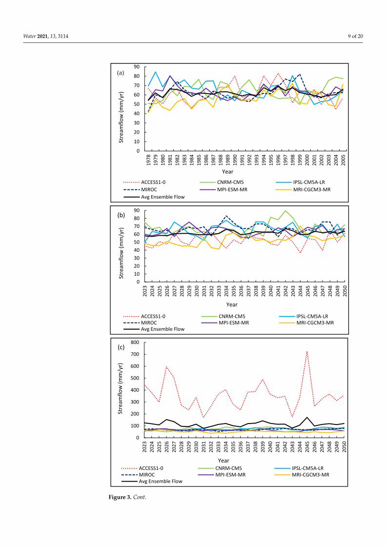
The different GCM projections were used as input for simulation of future streamflowby SWAT model for the baseline, RCP 4.5 and RCP 8.5 climate scenarios to show variationsand patterns. The results under RCP 8.5 were separated for strong consensus and highuncertainty to demonstrate future possibilities for the ZRB. The simulated results includethe calculated averages as shown in Figure 3a–d to highlight variations about the meanand patterns.

Water 2021, 13, 3114 9 of 20Water 2021, 13, x FOR PEER REVIEW 10 of 22

0

10

20

30

40

50

60

70

80

90

1978

1979

1980

1981

1982

1983

1984

1985

1986

1987

1988

1989

1990

1991

1992

1993

1994

1995

1996

1997

1998

1999

2000

2001

2002

2003

2004

2005

Stre

amflo

w (m

m/y

r)

Year

ACCESS1-0 CNRM-CM5 IPSL-CM5A-LRMIROC MPI-ESM-MR MRI-CGCM3-MRAvg Ensemble Flow

(a)

0102030405060708090

2023

2024

2025

2026

2027

2028

2029

2030

2031

2032

2033

2034

2035

2036

2037

2038

2039

2040

2041

2042

2043

2044

2045

2046

2047

2048

2049

2050

Stre

amflo

w (m

m/y

r)

Year

ACCESS1-0 CNRM-CM5 IPSL-CM5A-LRMIROC MPI-ESM-MR MRI-CGCM3-MRAvg Ensemble Flow

(b)

0

100

200

300

400

500

600

700

800

2023

2024

2025

2026

2027

2028

2029

2030

2031

2032

2033

2034

2035

2036

2037

2038

2039

2040

2041

2042

2043

2044

2045

2046

2047

2048

2049

2050

Stre

amflo

w (m

m/y

r)

YearACCESS1-0 CNRM-CM5 IPSL-CM5A-LRMIROC MPI-ESM-MR MRI-CGCM3-MRAvg Ensemble Flow

(c)

Figure 3. Cont.

Water 2021, 13, 3114 10 of 20Water 2021, 13, x FOR PEER REVIEW 11 of 22

Figure 3. (a) Baseline ensemble streamflow with the average; (b) RCP 4.5 ensemble streamflow with the average; (c) RCP 8.5 ensemble streamflow based on high uncertainty with the average; and (d) RCP 8.5 ensemble streamflow based on strong consensus with the average.

The streamflows based on the GCM baseline, the RCP 4.5 and RCP 8.5 strong con-sensus scenario in Figure 3a,b,d show similar patterns in the annual streamflow simula-tions that are in the same range of magnitude between 30 and 90 mm/year across the basin. Figure 3c indicates that the GCM ensemble was significantly different as the streamflow simulation based on Access1-0 is higher and in the range of 168–725 mm/year across the basin with a different pattern. The differences in simulations for RCP 8.5 may demonstrate uncertainty in non-perfectly calibrated model and GCMs that have various model charac-teristics [1].

3.4. Monthly Streamflow Analysis Figure 4a indicates the monthly streamflow, based on Access1–0 for the RCP 8.5 sce-

nario that has a high uncertainty, with the highest magnitude of 1696 m3/s compared to the baseline and RCP 4.5. The highest simulated streamflow occurs in January while, in February and March, the flow begins to recede until August, when it becomes similar to the base flow. The lowest flow of 204 m3/s is experienced in September and October. Thereafter, the flow begins to rise gently up to November, where there is a sharp rise due to rainfall events starting towards the end of September.

0

10

20

30

40

50

60

70

80

90

2023

2024

2025

2026

2027

2028

2029

2030

2031

2032

2033

2034

2035

2036

2037

2038

2039

2040

2041

2042

2043

2044

2045

2046

2047

2048

2049

2050

Stre

amflo

w (m

m/y

r)

YearCNRM-CM5 IPSL-CM5A-LR MIROCMPI-ESM-MR MRI-CGCM3-MR Avg Ensemble Flow

(d)

Figure 3. (a) Baseline ensemble streamflow with the average; (b) RCP 4.5 ensemble streamflow withthe average; (c) RCP 8.5 ensemble streamflow based on high uncertainty with the average; and(d) RCP 8.5 ensemble streamflow based on strong consensus with the average.

The streamflows based on the GCM baseline, the RCP 4.5 and RCP 8.5 strong consen-sus scenario in Figure 3a,b,d show similar patterns in the annual streamflow simulationsthat are in the same range of magnitude between 30 and 90 mm/year across the basin.Figure 3c indicates that the GCM ensemble was significantly different as the streamflowsimulation based on Access1-0 is higher and in the range of 168–725 mm/year across thebasin with a different pattern. The differences in simulations for RCP 8.5 may demon-strate uncertainty in non-perfectly calibrated model and GCMs that have various modelcharacteristics [1].

3.4. Monthly Streamflow Analysis

Figure 4a indicates the monthly streamflow, based on Access1–0 for the RCP 8.5scenario that has a high uncertainty, with the highest magnitude of 1696 m3/s comparedto the baseline and RCP 4.5. The highest simulated streamflow occurs in January while,in February and March, the flow begins to recede until August, when it becomes similarto the base flow. The lowest flow of 204 m3/s is experienced in September and October.Thereafter, the flow begins to rise gently up to November, where there is a sharp rise dueto rainfall events starting towards the end of September.

The peak baseline streamflow is 224 m3/s occurring in March while peak streamflowfor the RCP 4.5 scenario in the same month is 187 m3/s. The baseline streamflow isslightly higher than that of the RCP 4.5 throughout the year, predicting a decrease in flowmagnitude under RCP 4.5. The lowest flow for both baseline and RCP 4.5 is 73 m3/s inNovember. Figure 4a under RCP 8.5 (high uncertainty) shows a shift in the peak flowoccurrence when compared to the other three scenarios. The peak flow for RCP 8.5 inFigure 4a is predicted to be in January, while the baseline, RCP 4.5 and RCP 8.5 (Figure 4a’)scenarios have a corresponding peak flow in March. There is also a sharp rise in flowpredicted for the RCP 8.5 scenario for the period between November and January, whichmay be triggered by a high rainfall input at the beginning of October. Figure 4a’ indicatesthe monthly streamflow based on Access1-0 under RCP 4.5 and a baseline that has strongconsensus and shows similar pattern as all other GCM streamflows.

Water 2021, 13, 3114 11 of 20Water 2021, 13, x FOR PEER REVIEW 12 of 22

Figure 4. Streamflow simulations based on individual global climate models: (a) ACCESS1-0 (high uncertainty); (a′) AC-CESS1-0 (strong consensus); (b) CNRM-CM; (c) IPSL-CM5A-LR; (d) MIROC; (e) MPI-ESM-MR; (f) MRI-CGCM3-MR; and (g) average streamflow for GCM Ensemble.

0200400600800

10001200140016001800

Jan

Feb

Mar Ap

rM

ay Jun

Jul

Aug

Sep

Oct

Nov

DecStre

amflo

w (m

3/s)

Month Streamflow - BaselineStreamflow - RCP 4.5Streamflow - RCP 8.5

(a)

0

50

100

150

200

250

Jan

Feb

Mar Ap

rM

ay Jun

Jul

Aug

Sep

Oct

Nov

DecSt

ream

flow

(m3 /s

)

MonthStreamflow - BaselineStreamflow - RCP 4.5

(a')

050

100150200250300

Jan

Feb

Mar Ap

rM

ay Jun

Jul

Aug

Sep

Oct

Nov

DecSt

ream

flow

(m3 /s

)

MonthStreamflow - BaselineStreamflow - RCP 4.5Streamflow - RCP 8.5

(b)

050

100150200250300

Jan

Feb

Mar Ap

rM

ay Jun

Jul

Aug

Sep

Oct

Nov

DecSt

ream

flow

(m3 /s

)

MonthStreamflow - BaselineStreamflow - RCP 4.5Streamflow - RCP 8.5

(c)

050

100150200250300

Jan

Feb

Mar Apr

May Jun

Jul

Aug

Sep

Oct

Nov

DecSt

ream

flow

(m3 /s

)

MonthStreamflow - BaselineStreamflow - RCP 4.5Streamflow - RCP 8.5

(d)

050

100150200250300

Jan

Feb

Mar Ap

rM

ay Jun

Jul

Aug

Sep

Oct

Nov

DecSt

ream

flow

(m3 /s

)

MonthStreamflow - BaselineStreamflow - RCP 4.5Streamflow - RCP 8.5

(e)

050

100150200250

Jan

Feb

Mar Apr

May Jun

Jul

Aug

Sep

Oct

Nov

Dec

Stre

amflo

w (m

3 /s)

MonthStreamflow - BaselineStreamflow - RCP 4.5Streamflow - RCP 8.5

(f)

050

100150200250

Jan

Feb

Mar Ap

rM

ay Jun

Jul

Aug

Sep

Oct

Nov

DecStre

amflo

w(m

3 /s)

MonthAvg streamflow - BaselineAvg streamflow - RCP 4.5Avg streamflow - RCP 8.5

Figure 4. Streamflow simulations based on individual global climate models: (a) ACCESS1-0 (high uncertainty);(a′) ACCESS1-0 (strong consensus); (b) CNRM-CM; (c) IPSL-CM5A-LR; (d) MIROC; (e) MPI-ESM-MR; (f) MRI-CGCM3-MR;and (g) average streamflow for GCM Ensemble.

Water 2021, 13, 3114 12 of 20

Figure 4c shows the prediction of streamflow based on IPSL-CM5A-LR for the RCP4.5 and RCP 8.5 scenarios. The streamflow simulations have nearly the same flow regime,with some differences between January and April. The streamflow for RCP 8.5 is higherthan the ones for both RCP 4.5 and the baseline, which are almost comparable to oneanother throughout the year. Figure 4d shows the prediction of streamflow based onMIROC5 under the RCP 4.5 and RCP 8.5 scenarios compared to the baseline period. Thethree streamflow simulations have nearly the same magnitude and flow regime with somedifferences between January and April. The streamflow for RCP 8.5 is slightly higher thanfor RCP 4.5, which is also higher than the baseline streamflow between January and April.

Figure 4e shows no variation in the streamflow simulated for the baseline period, theRCP 4.5 and RCP 8.5 scenarios and therefore predicts no changes in streamflow for thenear future. Figure 4f shows the streamflow for RCP 4.5 and RCP 8.5 will be considerablyless between January to April, while slightly less for the rest of the months when comparedto the baseline.

Figure 4g shows the average streamflow for ensemble GCM based on baseline, RCP4.5 and RCP 8.5 with strong consensus. The streamflow simulation based on the GCMshows that the future magnitude of streamflow will reduce slightly between the months ofMay and December, while considerable reductions will occur between January and April.

Overall, Figure 4 shows most of the streamflow simulations, based on five GCM,predict slight increases in streamflow, while streamflow simulations based on Access1-0(Figure 4a) predict a considerable increase, and streamflow simulations based on MRI-CGCM3-MR predict slightly less streamflow. The streamflow simulations in Figure 4aare within the same range while streamflow simulations in Figure 4a have an enormousincrease when compared to other GCMs. Further analysis was therefore performed tocalculate monthly streamflow ensemble means based on the six GCM in Figure 5 for thebaseline as well as the RCP 4.5 and RCP 8.5 climate scenarios as it improves the outcome ofsimulations [46].

Water 2021, 13, x FOR PEER REVIEW 14 of 22

Figure 5. Monthly mean streamflow ensembles under (a) high uncertainty and (b) strong consensus.

The ensemble mean streamflow for RCP 8.5 indicates a sharp rise from November to January, while for RCP 4.5, there is a moderate rise from November to January. The pre-dictions from the ensemble mean streamflow indicate an increased magnitude of stream-flow for RCP 8.5, which may culminate into flooding of most parts of the basin depending on topography, whereas RCP 4.5 generally indicate a slightly lower streamflow when compared to the baseline flow. In order to determine the actual increase or decrease of the ensemble mean streamflow in Figure 6, the change factor methodology (CFM) [39] was applied.

Figure 6. Ensemble mean streamflow changes (a) under high uncertainty; and (b) strong consensus.

Figure 6a shows the highest streamflow of 270 m3/s for RCP 8.5, which is much higher than the ensemble means of that of RCP 4.5. The highest increase in streamflow occurs in January, while the lowest increase occurs in September and October. Prediction of the flow regime shows that peak flow occurs in January and recedes gently until September before beginning to rise again in November. Figure 6b shows the highest increase in streamflow of 25 m3/s for RCP 8.5 to be moderately higher than the streamflow for RCP 4.5.

3.5. Seasonal Flow Analysis The KRB experiences four seasons, namely December, January and February (DJF)

representing the typical rainy season (spring); March, April and May (MAM) indicating

0

50

100

150

200

250

Jan

Feb

Mar Ap

rM

ay Jun Jul

Aug

Sep

Oct

Nov

DecSt

ream

flow

(m3/

s)

MonthAvg streamflow - BaselineAvg streamflow - RCP 4.5Avg streamflow - RCP 8.5

(b)

Figure 5. Monthly mean streamflow ensembles under (a) high uncertainty and (b) strong consensus.

The mean streamflow ensembles shown in Figure 5a,b indicate that the baseline andRCP 4.5 streamflows will have insignificant variations in magnitude and flow regimealthough the stream flows for RCP 4.5 will be slightly less than baseline streamflow.Meanwhile, the mean streamflow for RCP 8.5 with high uncertainty will be much higher inmagnitude than the two ensemble mean streamflows with a wide variation in flow regime.The RCP 8.5 with strong consensus on Figure 5b shows a moderate increase in monthlystreamflow and with a similar pattern with Baseline and RCP 4.5 streamflow ensembles.The simulated flows are within the range of the other GCMs.

The ensemble mean streamflow for RCP 8.5 indicates a sharp rise from November toJanuary, while for RCP 4.5, there is a moderate rise from November to January. The predic-tions from the ensemble mean streamflow indicate an increased magnitude of streamflow

Water 2021, 13, 3114 13 of 20

for RCP 8.5, which may culminate into flooding of most parts of the basin dependingon topography, whereas RCP 4.5 generally indicate a slightly lower streamflow whencompared to the baseline flow. In order to determine the actual increase or decrease ofthe ensemble mean streamflow in Figure 6, the change factor methodology (CFM) [39]was applied.

Water 2021, 13, x FOR PEER REVIEW 14 of 22

Figure 5. Monthly mean streamflow ensembles under (a) high uncertainty and (b) strong consensus.

The ensemble mean streamflow for RCP 8.5 indicates a sharp rise from November to January, while for RCP 4.5, there is a moderate rise from November to January. The pre-dictions from the ensemble mean streamflow indicate an increased magnitude of stream-flow for RCP 8.5, which may culminate into flooding of most parts of the basin depending on topography, whereas RCP 4.5 generally indicate a slightly lower streamflow when compared to the baseline flow. In order to determine the actual increase or decrease of the ensemble mean streamflow in Figure 6, the change factor methodology (CFM) [39] was applied.

Figure 6. Ensemble mean streamflow changes (a) under high uncertainty; and (b) strong consensus.

0

50

100

150

200

250

Jan

Feb

Mar Ap

rM

ay Jun Jul

Aug

Sep

Oct

Nov

DecSt

ream

flow

(m3/

s)

MonthAvg streamflow - BaselineAvg streamflow - RCP 4.5Avg streamflow - RCP 8.5

(b)

Figure 6. Ensemble mean streamflow changes (a) under high uncertainty; and (b) strong consensus.

Figure 6a shows the highest streamflow of 270 m3/s for RCP 8.5, which is much higherthan the ensemble means of that of RCP 4.5. The highest increase in streamflow occurs inJanuary, while the lowest increase occurs in September and October. Prediction of the flowregime shows that peak flow occurs in January and recedes gently until September beforebeginning to rise again in November. Figure 6b shows the highest increase in streamflowof 25 m3/s for RCP 8.5 to be moderately higher than the streamflow for RCP 4.5.

3.5. Seasonal Flow Analysis

The KRB experiences four seasons, namely December, January and February (DJF)representing the typical rainy season (spring); March, April and May (MAM) indicatingthe autumn season; June, July and August (JJA) representing the winter season; and finally,September, October and November (SON) representing summer.

Streamflow varies depending on the season. DJF and MAM are known as wet sea-sons, while JJA and SON are known as dry seasons. Future streamflow from the GCMensemble means were analyzed based on the aforementioned seasons and monthly futurestreamflows. The CFM was applied to monthly streamflow and aggregated to seasonalstreamflow. Figure 7 shows the seasonal comparisons between baseline, RCP 4.5 and RCP8.5 stream flows under high uncertainty and strong consensus with corresponding changesper season.

Water 2021, 13, 3114 14 of 20

Water 2021, 13, x FOR PEER REVIEW 15 of 22

Figure 6a shows the highest streamflow of 270 m3/s for RCP 8.5, which is much higher than the ensemble means of that of RCP 4.5. The highest increase in streamflow occurs in January, while the lowest increase occurs in September and October. Prediction of the flow regime shows that peak flow occurs in January and recedes gently until September before beginning to rise again in November. Figure 6b shows the highest increase in streamflow of 25 m3/s for RCP 8.5 to be moderately higher than the streamflow for RCP 4.5.

3.5. Seasonal Flow Analysis The KRB experiences four seasons, namely December, January and February (DJF)

representing the typical rainy season (spring); March, April and May (MAM) indicating the autumn season; June, July and August (JJA) representing the winter season; and fi-nally, September, October and November (SON) representing summer.

Streamflow varies depending on the season. DJF and MAM are known as wet sea-sons, while JJA and SON are known as dry seasons. Future streamflow from the GCM ensemble means were analyzed based on the aforementioned seasons and monthly future streamflows. The CFM was applied to monthly streamflow and aggregated to seasonal streamflow. Figure 7 shows the seasonal comparisons between baseline, RCP 4.5 and RCP 8.5 stream flows under high uncertainty and strong consensus with corresponding changes per season.

Figure 7. Comparisons of change in seasonal streamflow for (a) high uncertainty; and (b) strong consensus.

The seasonal streamflow in Figure 7 indicates that for RCP 4.5, streamflow will be reduced by −0.6% in DJF, −0.7% in MAM, -1% in JJA and -2% in SON in both scenarios. The seasonal streamflow will be slightly less than the historical flow because all seasons have been predicted with an increasing negative magnitude, with highest occurrence in SON at 2% reduction.

However, the seasonal streamflow for RCP 8.5 is apparently high for all seasons in contrast to the baseline and RCP 4.5 stream flows. The highest seasonal streamflow change in Figure 7a is predicted to be 134% for DJF, which is followed by 87% for MAM, 44% for JJA and 34% for SON. This implies that DJF and MAM may experience severe floods, whereas JJA and SON represent the dry season where the streamflow does not signifi-cantly differ from the baseline flow. Predictions in Figure 7b show that seasonal stream-flow will increase in DJF by 10%, MAM by 5%, JJA by 2% and SON by 5%. All percentage calculations are based on baseline data.

The results show consistency with previous studies which predicted that, under the RCP 8.5 scenario for the period 2020–2050, most part of the ZRB is likely to experience dryness, apart from areas in the north (close to Malawi and Northern Zambia), which will

-5

15

35

55

75

95

115

135

DJF MAM JJA SON

Stre

amflo

w ch

ange

%

SeasonRCP 8.5 Seasonal streamflow changeRCP 4.5 Seasonal streamflow change

(a)

-2

0

2

4

6

8

10

DJF MAM JJA SON

Stre

amflo

w C

hang

e (%

)

SeasonRCP 8.5 Seasonal streamflow changeRCP 4.5 Seasonal streamflow change

Figure 7. Comparisons of change in seasonal streamflow for (a) high uncertainty; and (b) strong consensus.

The seasonal streamflow in Figure 7 indicates that for RCP 4.5, streamflow will bereduced by −0.6% in DJF, −0.7% in MAM, −1% in JJA and −2% in SON in both scenarios.The seasonal streamflow will be slightly less than the historical flow because all seasonshave been predicted with an increasing negative magnitude, with highest occurrence inSON at 2% reduction.

However, the seasonal streamflow for RCP 8.5 is apparently high for all seasons incontrast to the baseline and RCP 4.5 stream flows. The highest seasonal streamflow changein Figure 7a is predicted to be 134% for DJF, which is followed by 87% for MAM, 44% for JJAand 34% for SON. This implies that DJF and MAM may experience severe floods, whereasJJA and SON represent the dry season where the streamflow does not significantly differfrom the baseline flow. Predictions in Figure 7b show that seasonal streamflow will increasein DJF by 10%, MAM by 5%, JJA by 2% and SON by 5%. All percentage calculations arebased on baseline data.

The results show consistency with previous studies which predicted that, under theRCP 8.5 scenario for the period 2020–2050, most part of the ZRB is likely to experiencedryness, apart from areas in the north (close to Malawi and Northern Zambia), which willbe wetter and therefore leading to high streamflow [15,17]. As the KRB is located in theNorth-western part of Zambia, the results agree with the findings on the rise of extremeevents in most ZRB riparian states that included Malawi, Zambia and Mozambique [47].Others previous studies predicted a significant increase in rainfall events over SouthernAfrica (including Angola, Namibia, Mozambique, Malawi and Zambia), which will lead tomore streamflow [48,49].

3.6. Intra-Annual Flow Analysis

Concerning the monthly streamflow simulation for six GCM, the intra-annual variabil-ity showed a uniform pattern of streamflow indicating significant correlation efficiency. Thestreamflow simulation in Figure 8 shows monthly streamflow variability for six GCM basedon RCP 8.5 and with significant differences between high uncertainty and strong consensus.

The simulated streamflow in Figure 8a shows that monthly streamflow for Access1.0 ismuch higher than the majority, suggesting uncertainty and confirming that different GCMrespond differently to model formulations for dynamics, physics (i.e., parameterizations)and external forcing. Figure 8b shows that the simulations from the GCM are similarand give a uniform pattern throughout the period of projection. The simulated monthlyflows were aggregated to ensemble mean annual flows in Figure 9 to analyze the annualvariability for the three climate scenarios.

Water 2021, 13, 3114 15 of 20

Water 2021, 13, x FOR PEER REVIEW 16 of 22

be wetter and therefore leading to high streamflow [15,17]. As the KRB is located in the North-western part of Zambia, the results agree with the findings on the rise of extreme events in most ZRB riparian states that included Malawi, Zambia and Mozambique [47]. Others previous studies predicted a significant increase in rainfall events over Southern Africa (including Angola, Namibia, Mozambique, Malawi and Zambia), which will lead to more streamflow [48,49].

3.6. Intra-Annual Flow Analysis Concerning the monthly streamflow simulation for six GCM, the intra-annual varia-

bility showed a uniform pattern of streamflow indicating significant correlation efficiency. The streamflow simulation in Figure 8 shows monthly streamflow variability for six GCM based on RCP 8.5 and with significant differences between high uncertainty and strong consensus.

Figure 8. Monthly streamflow for RCP 8.5 for (a) high uncertainty; and (b) strong consensus. Figure 8. Monthly streamflow for RCP 8.5 for (a) high uncertainty; and (b) strong consensus.

The ensemble mean annual flows in Figure 9a are predicted to be high for RCP 8.5with high uncertainty compared to the ensemble mean for both RCP 4.5 and baseline.Figure 9a shows that annual flows for RCP 4.5 and baseline have insignificant differences inmagnitude and regime. The ensemble mean annual streamflow for RCP 4.5 in Figure 9a,bpredicts a slight reduction when compared to the baseline streamflow. This result isconsistent with the previous study which predicted that on average the annual rainfallin the ZRB (about 960 mm) will decrease across the ZRB, which is expected to reducerunoff [16], while others predicted from the baseline runoff data that it will decrease by2050s [44]. Researchers predicted that ZRB would result in a decline in water runoff withconsequent reductions in streamflow under RCP 4.5 by 2100 [49].

Water 2021, 13, 3114 16 of 20

Water 2021, 13, x FOR PEER REVIEW 17 of 22

The simulated streamflow in Figure 8a shows that monthly streamflow for Access1.0 is much higher than the majority, suggesting uncertainty and confirming that different GCM respond differently to model formulations for dynamics, physics (i.e., parameteri-zations) and external forcing. Figure 8b shows that the simulations from the GCM are similar and give a uniform pattern throughout the period of projection. The simulated monthly flows were aggregated to ensemble mean annual flows in Figure 9 to analyze the annual variability for the three climate scenarios.

Figure 9. Ensemble mean annual flows for (a) high uncertainty; and (b) strong consensus.

The ensemble mean annual flows in Figure 9a are predicted to be high for RCP 8.5 with high uncertainty compared to the ensemble mean for both RCP 4.5 and baseline. Figure 9a shows that annual flows for RCP 4.5 and baseline have insignificant differences

Figure 9. Ensemble mean annual flows for (a) high uncertainty; and (b) strong consensus.

3.7. Intra-Annual and Inter-Annual Streamflow Variability

Flow regime analysis has always been critical in the environmental sciences to en-hance the understanding of streamflow variability [50]. Intra-annual variability of baseline,RCP 4.5 and RCP 8.5 stream flows were determined for each GCM to assess the distri-bution around the mean, which was calculated as Coefficient of Variation (CV). Table 1indicates the estimated CV for various stream flows for different climate scenarios. Allthe CVs for the RCP 4.5 scenario are lower than that of the baseline scenario. Therefore,

Water 2021, 13, 3114 17 of 20

most simulations indicate that intra-annual and inter-annual streamflow variabilities willdecrease for RCP 4.5 in the future.

Table 1. Estimated coefficient of variation (CV).

GCM. Access CNRMCM5

IPSLCM5A

LRMIROC MPI-ESM-MR MRI-CGCM3-MR Highest

CVMean

CVLowest

CV

Baseline scenarioIntra-annual CV 0.410 0.413 0.404 0.387 0.386 0.396 0.413 0.399 0.386Inter-annual CV 0.160 0.139 0.140 0.128 0.096 0.153 0.160 0.136 0.096

RCP 4.5 ScenarioIntra-annual CV 0.399 0.401 0.419 0.406 0.384 0.371 0.419 0.397 0.371Inter-annual CV 0.141 0.121 0.119 0.087 0.079 0.125 0.141 0.112 0.079

RCP 8.5 ScenarioIntra-annual CV 0.998 0.427 0.434 0.419 0.407 0.375 0.998 0.510 0.375Inter-annual CV 0.334 0.158 0.118 0.101 0.116 0.142 0.334 0.161 0.101

Most of the CVs for the RCP 8.5 scenario (except those for MRI-CGCM3-MR) arehigher than the CVs for the baseline scenario. The annual streamflow increase is ratherhigh and has, therefore, been assessed by investigating the intra-annual and inter-annualvariability of streamflow, which was high for RCP 8.5.

Table 1 shows that the averaged intra-annual variability for RCP 8.5 for high uncer-tainty is 0.510, which is higher than 0.399 of the six estimates of the intra-annual variabilityfor the baseline. Similarly, the averaged inter-annual variability for RCP 8.5 for high un-certainty is 0.161, which is also higher than 0.136 of the six estimates of the inter-annualvariability for the baseline. In the same way, most of the CV for the RCP 8.5 scenario(except those for MRI-CGCM3-MR) are higher than the CV for the baseline scenario. Mostsimulations indicate that intra-annual and inter-annual streamflow variability will increasein the future for RCP 8.5 by a considerable margin.

The results revealed a huge uncertainty of the future for the KRB. The KRB is facedwith two scenarios based on RCP 8.5 which is the unrestricted policy for high uncertaintyand strong consensus with implications for floods and drought, respectively. The overviewof results analysed under high uncertainty show that climate change may result in floodsin the basin. The KRB baseline period shows years of floods and drought that have beenreported in the past. The predicted potential floods are expected to be more severe thanthe historical floods. This may lead to more severe damage to infrastructure, food crops,ecosystems, and possibly loss of lives if adequate adaptation and mitigation strategiesare not put in place. Water quality is also likely to be altered and more low-lying areasare expected to be inundated. The predicted high temperatures in the basin may haveimplications of high evapotranspiration from vegetation and high evaporation from surfacewater bodies. This scenario requires strengthening of flood early warning systems to helpin adaptation and mitigation.

The climate change scenario under strong consensus shows a status quo where stream-flow is likely to remain the same. However, the basin water resources may be more stresseddue to the increased water demand and possible rise in evapotranspiration. The scenarioof drought will culminate into high aridity and drying up of some rivers and streams, aswell as boreholes, leading to water shortages in some communities that largely dependon groundwater points. Agriculture productivity may be negatively affected and lead tofood insecurity. Water levels in reservoirs may drastically be reduced affecting hydropowergeneration capacity and therefore subsequently affecting the ecosystem, some miningactivities, water supply, and small-scale industries in KRB.

3.8. Main Limitations of the Study

The GCM, Access1-0 under RCP 8.5 had simulated higher magnitudes of streamflowcompared to the other five GCMs, indicating uncertainties, and a conclusion was madebased on strong consensus and high uncertainty. The streamflow results for RCP 8.5

Water 2021, 13, 3114 18 of 20

showed uncertainty in magnitude, which was also observed by other researchers whostated that there is uncertainty in magnitude and direction of change in the Zambezi Riverbasin response to future GCM projections [43,44]. It was pointed out that GCM runsperformed under RCP 8.5 result in more uncertainty than under RCP 4.5 because of climatedistribution [17]. The simulation of Access1-0 under RCP 8.5 was considered to be a uniquemodel skill (1).

4. Conclusions

The detailed analysis of streamflow under high resolution for strong consensus andhigh uncertainty is considered a novelty. The generated new knowledge for streamflowvariability under various scenarios could be useful for future water resources planning andcontribute to the preparation of realistic adaptation measures for the basin.

The projected changes in temperature show an increasing trend with minor uncertain-ties, while showing considerable uncertainties in precipitation. The basin for the RCP 8.5scenario shows significant changes in streamflow based on high uncertainty and strongconsensus among the ensemble streamflow simulations and strong consensus where thefive GCM streamflow have good agreement. There are also significant increases in seasonalstream flows that range between 34% and 134% as analyzed from the ensemble mean ofRCP 8.5 under high uncertainty, while the seasonal increases under the strong consensusrange between 2% and 10%

The basin for the RCP 4.5 scenario will be subjected to insignificant changes in monthly,seasonal and annual flow regimes and magnitudes. The predictions suggest that themagnitude and temporal streamflow will be slightly less than the baseline magnitude. TheRCP 4.5 future climate scenario predicts a negligible reduction in streamflow for the basinwhether simulated as individual GCM or ensemble mean.

The predicted high stream flows for RCP 8.5 under high uncertainty and moderaterise in stream flow under strong consensus suggest the need for adaptation plans andmitigation strategies. In contrast, the stream flows predicted for RCP 4.5 will requirethe review of current management strategies of water resources in the basin, consideringthe ever-increasing water demand and other impacts, such as on water quality. Mostsimulations indicate that intra-annual and inter-annual streamflow variability will decreasein the future for RCP 4.5, while increasing for RCP 8.5 for both cases (high uncertainty andstrong consensus) by a considerable margin.

Temperature was predicted with a robust change signal, while precipitation was veryvariable with huge uncertainties, especially for the RCP 8.5 scenario. The future studiesneed to focus on RCP 4.5 and RCP 8.5 for the period 2050–2090 to assess any possibleclimate change impacts, such as temperature change on streamflow, that would arise fromthe corresponding scenarios. It is also recommended to analyse the effects of landuse/landcover changes on water resources and to increase the number of GCM projections tofind a better consensus and possible uncertainty for analysis of future hydrology andwater resources.

Author Contributions: Conceptualization, G.Z.N. and Y.E.W.; methodology, G.Z.N. and Y.E.W.;software, G.Z.N.; validation, G.Z.N. and Y.E.W.; formal analysis, G.Z.N. and Y.E.W.; investigation,G.Z.N. and Y.E.W.; data curation, G.Z.N.; writing—original draft preparation, G.Z.N.; writing—review and editing, Y.E.W.; visualization, G.Z.N. All authors have read and agreed to the publishedversion of the manuscript.

Funding: This research received no external funding.

Institutional Review Board Statement: Not applicable.

Informed Consent Statement: Not applicable.

Data Availability Statement: Available upon a request from corresponding author.

Acknowledgments: We sincerely thank Central University of Technology, Free State, for the support.

Water 2021, 13, 3114 19 of 20

Conflicts of Interest: The authors declare no conflict of interest.

References1. Lutz, A.F.; ter Maat, H.W.; Biemans, H.; Shrestha, A.B.; Wester, P.; Immerzeel, W.W. Selecting representative climate models for

climate change impact studies: An advanced envelope-based selection approach. Int. J. Clim. 2016, 36, 3988–4005. [CrossRef]2. Chien, H.; Yeh, P.J.-F.; Knouft, J.H. Modeling the potential impacts of climate change on streamflow in agricultural watersheds of

the Midwestern United States. J. Hydrol. 2013, 491, 73–88. [CrossRef]3. Kusangaya, S.; Warburton, M.L.; van Garderen, E.A.; Jewitt, G. Impacts of climate change on water resources in southern Africa:

A review. Phys. Chem. Earth Parts A/B/C 2014, 67–69, 47–54. [CrossRef]4. Goosse, H.; Barriat, P.Y.; Lefebvre, W.; Loutre, M.F.; Zunz, V. Modelling the Climate System. In Introduction to Climate Dynamics

and Climate Modeling; Universite Catholique de Louvain: Louvain, Belgium, 2010; Chapter 3; pp. 59–86. ISBN 9781107445833.Available online: http://www.climate.be/textbook (accessed on 4 February 2021).

5. Moss, R.H.; Edmonds, J.A.; Hibbard, K.A.; Manning, M.R.; Rose, S.K.; van Vuuren, D.P.; Carter, T.R.; Emori, S.; Kainuma, M.;Kram, T.; et al. The next generation of scenarios for climate change research and assessment. Nat. Cell Biol. 2010, 463, 747–756.[CrossRef] [PubMed]

6. Meinshausen, M.; Smith, S.J.; Calvin, K.; Daniel, J.S.; Kainuma, M.L.T.; Lamarque, J.F.; Matsumoto, K.; Montzka, S.A.; Raper,S.C.B.; Riahi, K.; et al. The RCP greenhouse gas concentrations and their extensions from 1765 to 2300. Clim. Chang. 2011, 109,213–241. [CrossRef]

7. Van Vuuren, D.P.; Edmonds, J.; Kainuma, M.; Riahi, K.; Thomson, A.; Hibbard, K.; Hurtt, G.C.; Kram, T.; Krey, V.;Lamarque, J.-F.; et al. The representative concentration pathways: An overview. Clim. Chang. 2011, 109, 5–31. [CrossRef]

8. Musie, M.; Sen, S.; Srivastava, P. Application of CORDEX-AFRICA and NEX-GDDP datasets for hydrologic projections underclimate change in Lake Ziway sub-basin, Ethiopia. J. Hydrol. Reg. Stud. 2020, 31, 100721. [CrossRef]

9. Murthy, C. Climate Change and Catchment Hydrology. Irish Climate Analysis and Research Unit (ICARUS); Department of Geography,National University of Ireland: Maynooth, Ireland, 2012. Available online: http://mural.maynoothuniversity.ie/4890/1/CM_Climate_Change.pdf (accessed on 10 January 2020).

10. Fan, F.M.; Collischonn, W.; Meller, A.; Botelho, L.C.M. Ensemble streamflow forecasting experiments in a tropical basin: The SãoFrancisco river case study. J. Hydrol. 2014, 519, 2906–2919. [CrossRef]

11. Saddique, N.; Usman, M.; Bernhofer, C. Simulating the Impact of Climate Change on the Hydrological Regimes of a SparselyGauged Mountainous Basin, Northern Pakistan. Water 2019, 11, 2141. [CrossRef]

12. Gosling, S.N.; Taylor, R.G.; Arnell, N.W.; Todd, M.C. A comparative analysis of projected impacts of climate change on riverrunoff from global and catchment-scale hydrological models. Hydrol. Earth Syst. Sci. 2011, 15, 279–294. [CrossRef]

13. Lespinas, F.; Ludwig, W.; Heussner, S. Hydrological and climatic uncertainties associated with modeling the impact of climatechange on water resources of small Mediterranean coastal rivers. J. Hydrol. 2014, 511, 403–422. [CrossRef]

14. Li, Z.; Jin, J. Evaluating climate change impacts on streamflow variability based on a multisite multivariate GCM downscalingmethod in the Jing River of China. Hydrol. Earth Syst. Sci. 2017, 21, 5531–5546. [CrossRef]

15. Gautam, S.; Costello, C.; Baffaut, C.; Thompson, A.; Svoma, B.M.; Phung, Q.A.; Sadler, E.J. Assessing Long-Term HydrologicalImpact of Climate Change Using an Ensemble Approach and Comparison with Global Gridded Model-A Case Study onGoodwater Creek Experimental Watershed. Water 2018, 10, 564. [CrossRef]

16. Hamududu, B.H. Impacts of Climate Change on Water Resources and Hydropower Systems in Central and Southern Africa; NorwegianUniversity of Science and Technology: Trondheim, Norway, 2012.

17. Fant, C.; Gebretsadik, Y.; McCluskey, A.; Strzepek, K. An uncertainty approach to assessment of climate change impacts on theZambezi River Basin. Clim. Chang. 2015, 130, 35–48. [CrossRef]

18. Githui, F.; Gitau, W.; Mutua, F.; Bauwens, W. Climate change impact on SWAT simulated streamflow in western Kenya. Int. J.Clim. 2009, 29, 1823–1834. [CrossRef]

19. Ndhlovu, G.; Woyessa, Y. Modelling impact of climate change on catchment water balance, Kabompo River in Zambezi RiverBasin. J. Hydrol. Reg. Stud. 2019, 27, 100650. [CrossRef]

20. Ngongondo, C.; Li, L.; Gong, L.; Xu, C.-Y.; Alemaw, B.F. Flood frequency under changing climate in the upper Kafue River basin,southern Africa: A large scale hydrological model application. Stoch. Environ. Res. Risk Assess. 2013, 27, 1883–1898. [CrossRef]

21. Ndhlovu, G.; Woyessa, Y. Use of gridded climate data for hydrological modelling in the Zambezi River Basin, Southern Africa. J.Hydrol. 2021, 602, 126749. [CrossRef]

22. World Bank. The Zambezi River Basin—A Multi-Sector Investment Opportunity Analysis; The World Bank: Washington, DC, USA,2010. Available online: http://documents.worldbank.org/curated/en/724861468009989838/Summary-report (accessed on12 October 2018).

23. Kapangaziwiri, E.; Mokoena, M.P.; Kahinda, J.M.; Hughes, D.A. An Evaluation for Use in South Africa. WRC Report; ECOMAG;Water Research Commission: Gezina, South Africa, 2013; pp. 1–59.

24. Young, T.; Tucker, T.; Galloway, M.; Manyike, P. Climate Change and Health in SADC. (September). 2010. Available online:http://www.sead.co.za/downloads/climate-change-2010.pdf (accessed on 12 December 2019).

25. Moriasi, D.N.; Arnold, J.G.; Van Liew, M.W.; Bingner, R.L.; Harmel, R.D.; Veith, T.L. Model Evaluation Guidelines for SystematicQuantification of Accuracy in Watershed Simulations. Trans. Am. Soc. Agric. Biol. Eng. 2007, 50, 885–900. [CrossRef]

Water 2021, 13, 3114 20 of 20

26. Gassman, P.W.; Reyes, M.R.; Green, C.H.; Arnold, J.G. The Soil and Water Assessment Tool: Historical Development, Applications,and Future Research Directions. Trans. ASAE 2007, 50, 1211–1250. [CrossRef]

27. Neitsch, S.L.; Arnold, J.G.; Kiniry, J.R.; Williams, J.R. Soil and Water Assessment Tool User’s Manual Version 2005. In Proceedingsof the Diffuse Pollution Conference, Dublin, Ireland, 26 June–1 July 2005.

28. Arnold, J.G.; Moriasi, D.N.; Gassman, P.W.; Abbaspour, K.C.; White, M.J.; Srinivasan, R.; Santhi, C.; Harmel, R.D.; van Griensven,A.; Van Liew, M.W.; et al. SWAT: Model Use, Calibration, and Validation. Trans. ASABE 2012, 55, 1491–1508. [CrossRef]

29. Winchell, M.; Srinivasan, R.; Di Luzio, M.; Arnold, J.G. Arcswat Interface for SWAT2012: User’s Guide. Blackland Research Center,Texas AgriLife Research, College Station, pp. 1–464. Available online: https://www.scirp.org/(S(351jmbntvnsjt1aadkposzje))/reference/ReferencesPapers.aspx?ReferenceID=1935534 (accessed on 12 September 2021).

30. Waichler, S.R.; Wigmosta, M.S. Waichler, S.R.; Wigmosta, M.S. Development of hourly meteorological values from daily data andsignificance to hydrological modeling at HJ Andrews Experimental Forest. J. Exp. Forest. J. Hydromet 2003, 4, 251–263. [CrossRef]

31. Mehan, S.; Guo, T.; Gitau, M.W.; Flanagan, D.C. Comparative Study of Different Stochastic Weather Generators for Long-TermClimate Data Simulation. Climate 2017, 5, 26. [CrossRef]

32. Taylor, K.E.; Stouffer, R.J.; Meehl, G.A. An Overview of CMIP5 and the Experiment Design. Bull. Am. Meteorol. Soc. 2012, 93,485–498. [CrossRef]

33. Khan, N.; Shahid, S.; Ahmed, K.; Ismail, T.; Nawaz, N.; Son, M. Performance Assessment of General Circulation Model inSimulating Daily Precipitation and Temperature Using Multiple Gridded Datasets. Water 2018, 10, 1793. [CrossRef]

34. NASA. NASA Earth Exchange Global Daily Downscaled Projections (NEX-GDDP) 1, 2015. Intent of This Document and POC.2020. Available online: https://www.nccs.nasa.gov/services/data-collections/land-based-products/nex-gddp (accessed on5 April 2020).

35. Abbaspour, K.C.; Rouholahnejad, E.; Vaghefi, S.; Srinivasan, R.; Yang, H.; Kløve, B. A continental-scale hydrology and waterquality model for Europe: Calibration and uncertainty of a high-resolution large-scale SWAT model. J. Hydrol. 2015, 524, 733–752.[CrossRef]

36. Mei, Y.; Nikolopoulos, E.I.; Anagnostou, E.N.; Borga, M. Evaluating Satellite Precipitation Error Propagation in Runoff Simulationsof Mountainous Basins. J. Hydrometeorol. 2016, 17, 1407–1423. [CrossRef]

37. Khan, R.S.; Bhuiyan, M.A.E. Artificial Intelligence-Based Techniques for Rainfall Estimation Integrating Multisource PrecipitationDatasets. Atmosphere 2021, 12, 1239. [CrossRef]

38. Krysanova, V.; Donnelly, C.; Gelfan, A.; Gerten, D.; Arheimer, B.; Hattermann, F.; Kundzewicz, Z.W. How the performance ofhydrological models relates to credibility of projections under climate change. Hydrol. Sci. J. 2018, 63, 696–720. [CrossRef]

39. Anandhi, A.; Frei, A.; Pierson, D.C.; Schneiderman, E.M.; Zion, M.S.; Lounsbury, D.; Matonse, A.H. Examination of change factormethodologies for climate change impact assessment. Water Resour. Res. 2011, 47, 1–10. [CrossRef]

40. Nash, J.; Sutcliffe, J. River flow forecasting through conceptual models part I—A discussion of principles. J. Hydrol. 1970, 10,282–290. [CrossRef]

41. Tan, M.L.; Gassman, P.W.; Cracknell, A.P. Assessment of Three Long-Term Gridded Climate Products for Hydro-ClimaticSimulations in Tropical River Basins. Water 2017, 9, 229. [CrossRef]

42. Narsimlu, B.; Gosain, A.K.; Chahar, B.R.; Singh, S.K.; Srivastava, P.K. SWAT Model Calibration and Uncertainty Analysis forStreamflow Prediction in the Kunwari River Basin, India, Using Sequential Uncertainty Fitting. Environ. Process 2015, 2, 79–95.[CrossRef]

43. Banze, F.; Guo, J.; Xiaotao, S. Variability and trends of rainfall, precipitation and discharges over zambezi river basin, southernafrica: Review. Int. J. Hydrol. 2018, 2, 1. [CrossRef]

44. Tirivarombo, S. Hydrological Impacts of Climate Change in The Zambezi River Basin. Int. J. Sci. Res. Innov. Technol. 2017, 4,60–75.

45. Hidalgo, H.G.; Das, T.; Dettinger, M.D.; Cayan, D.R.; Pierce, D.W.; Barnett, T.P.; Bala, G.; Mirin, A.A.; Wood, A.; Bonfils, C.; et al.Detection and Attribution of Streamflow Timing Changes to Climate Change in the Western United States. J. Clim. 2009, 22,3838–3855. [CrossRef]

46. Garcia, R.A.; Burgess, N.D.; Cabeza, M.; Rahbek, C.; Araújo, M.B. Exploring consensus in 21st century projections of climaticallysuitable areas for African vertebrates. Glob. Chang. Biol. 2012, 18, 1253–1269. [CrossRef]

47. Tadross, M.; Suarez, P.; Lotsch, A.; Hachigonta, S.; Mdoka, M.; Unganai, L.; Muchinda, M. Changes in grow-ing-season rainfallcharacteristics and downscaled scenarios of change over southern Africa: Implications for growing maize. In IPCC RegionalExpert Meeting on Regional Impacts, Adaptation, Vulnerability, and Mitigation; IPCC: Nadi, Fiji, 2015; pp. 193–204. Available online:https://www.researchgate.net/publication/266465938 (accessed on 7 March 2021).

48. Usman, M.; Reason, C. Dry spell frequencies and their variability over southern Africa. Clim. Res. 2004, 26, 199–211. [CrossRef]49. Maure, G.A.; Pinto, I.; Ndebele-Murisa, M.R.; Muthige, M.; Lennard, C.; Nikulin, G.; Dosio, A.; Meque, A.O. The southern African

climate under 1.5 ◦C and 2 ◦C of global warming as simulated by CORDEX regional climate models. Environ. Res. Lett. 2018, 13,065002. [CrossRef]

50. Berhanu, B.; Seleshi, Y.; Demisse, S.S.; Melesse, A.M. Flow Regime Classification and Hydrological Characterization: A CaseStudy of Ethiopian Rivers. Water 2015, 7, 3149–3165. [CrossRef]