PUBLISHED VERSION

Westra, Seth Pieter; Sharma, Ashish; Brown, Casey; Lall, Upmanu Multivariate streamflow forecasting using independent component analysis Water Resources Research, 2008; 44:W02437

Copyright 2008 by the American Geophysical Union

http://hdl.handle.net/2440/72513

PERMISSIONS

http://www.agu.org/pubs/authors/usage_permissions.shtml

AGU allows authors to deposit their journal articles if the version is the final published citable version of record, the AGU copyright statement is clearly visible on the posting, and the posting is made 6 months after official publication by the AGU.

date ‘rights url’ accessed:15 August 2012

Multivariate streamflow forecasting using independent

component analysis

Seth Westra,1,3 Ashish Sharma,1 Casey Brown,2 and Upmanu Lall2

Received 10 April 2007; revised 26 September 2007; accepted 9 November 2007; published 27 February 2008.

[1] Seasonal forecasting of streamflow provides many benefits to society, by improvingour ability to plan and adapt to changing water supplies. A common approach todeveloping these forecasts is to use statistical methods that link a set of predictorsrepresenting climate state as it relates to historical streamflow, and then using this model toproject streamflow one or more seasons in advance based on current or a projected climatestate. We present an approach for forecasting multivariate time series using independentcomponent analysis (ICA) to transform the multivariate data to a set of univariate timeseries that are mutually independent, thereby allowing for the much broader class ofunivariate models to provide seasonal forecasts for each transformed series. Uncertainty isincorporated by bootstrapping the error component of each univariate model so that theprobability distribution of the errors is maintained. Although all analyses are performedon univariate time series, the spatial dependence of the streamflow is captured byapplying the inverse ICA transform to the predicted univariate series. We demonstrate thetechnique on a multivariate streamflow data set in Colombia, South America, bycomparing the results to a range of other commonly used forecasting methods. The resultsshow that the ICA-based technique is significantly better at representing spatialdependence, while not resulting in any loss of ability in capturing temporal dependence.As such, the ICA-based technique would be expected to yield considerable advantageswhen used in a probabilistic setting to manage large reservoir systems with multipleinflows or data collection points.

Citation: Westra, S., A. Sharma, C. Brown, and U. Lall (2008), Multivariate streamflow forecasting using independent component

analysis, Water Resour. Res., 44, W02437, doi:10.1029/2007WR006104.

1. Introduction

[2] Providing seasonal forecasts of rainfall and/or stream-flow is an important challenge in hydrology, with potentialbenefits in reservoir management, operation of irrigationnetworks, and flood control, among others. These forecastscan be particularly pertinent for regions that experiencesignificant inter-annual variability that result from theEl Nino Southern Oscillation (ENSO) phenomenon [Chiewand McMahon, 2002; Sharma, 2000a], as it is often possibleto use knowledge of ENSO and related oceanic patterns toprovide estimates of future rainfall and/or streamflow thatoutperform the climatological means. Although societalbenefits of these forecasts can be difficult to quantify,several studies have been published recently showing sig-nificant economic gains through the application of suchforecasts to hydropower generation [e.g., Hamlet et al.,2002; Yao and Georgakakos, 2001].[3] These forecasts are commonly classified as either

statistical or dynamical, with an excellent review provided

by Goddard et al. [2001]. The present paper concerns itselfwith the field of statistical forecasts, which involves identi-fying mathematical relationships between a set of predictorssuch as global sea surface temperatures (SSTs), and thevariables one wishes to predict (predictands), which for waterresources applications typically includes rainfall and/orstreamflow at a catchment or regional scale. To be consideredsuccessful, these forecasts generally are expected at mini-mum to outperform the climatological mean, as well aspredictions obtained by adopting a simple persistence modelthat assumes recent climate anomalies will continue into thefollowing season [Huang et al., 1996].[4] A review of a large number of statistical forecast

models around the world [Goddard et al., 2001] suggeststhat most of the predictability from these models is relatedto variability in the tropical Pacific, and in particular inrelation to the ENSO phenomenon [for example, seeBarnston, 1994; Casey, 1998; Chiew and McMahon,2002; Filho and Lall, 2003]. Thus it has become commonto use indices of ENSO as the basis of the statistical model.Popular forms of such models include either parametric[e.g., McBride and Nicholls, 1983; Singhrattna et al., 2005;Woolddridge et al., 1999] or non-parametric [e.g., Sharma,2000b; Singhrattna et al., 2005] regression models, condi-tional probabilitymodels (by defining a given year as ElNino,La Nina or neutral, and estimating the conditional probabilitydensity function of the predictand according to this classifi-

1School of Civil and Environmental Engineering, The University of NewSouth Wales, Sydney, NSW, Australia.

2Department of Earth and Environmental Engineering, ColumbiaUniversity, New York, New York, USA.

3Now at Sinclair Knight Merz, NSW, Australia.

Copyright 2008 by the American Geophysical Union.0043-1397/08/2007WR006104$09.00

W02437

WATER RESOURCES RESEARCH, VOL. 44, W02437, doi:10.1029/2007WR006104, 2008ClickHere

for

FullArticle

1 of 11

cation; see Mason and Goddard, 2001; by defining a givenyear as El Nino, La Nina or neutral, and estimating theconditional probability density function of the predictandaccording to this classification; see Ropelewski and Halpert,1996), andmodels that incorporate both ENSOstate aswell asa recent trend component [Stone et al., 1996].[5] In numerous instances, one may wish to consider

climate features which are not adequately described by oneof the ENSO indices as potential predictors to a statisticalmodel [e.g., Verdon et al., 2004]. These additional featuresmay be described by other indices, such as the NorthAtlantic Oscillation [NAO; Hurrell, 1995; Hurrell andVan Loon, 1997] or the Indian Ocean Dipole [IOD; Ashoket al., 2003; IOD; Saji et al., 1999; Saji and Yamagata,2003], however these indices represent climatological phe-nomena which are themselves often highly correlated withENSO. An alternative to the index-based approach makesuses information contained in the large multivariate datasets such as global sea surface temperatures (SSTs), whichhas been shown to enhance the quality of forecasts innumerous instances [e.g., Drosdowsky and Chambers,2001; Nicholls, 1989].[6] As these global data fields are usually quite large, and

contain significant spatial correlation, some form of dimen-sion reduction is required prior to incorporation into astatistical model. In simple cases, this might involve appli-cation of principal components analysis (PCA) to themultivariate predictor data set to extract individual ‘modes’of variability that are mutually uncorrelated and successivelyexplain the maximum amount of remaining variance in thedata [Barnston and Ropelewski, 1992]. This is frequentlyfollowed by applying a rotation to the PCA solution toenhance interpretability of the climate ‘modes’, with Varimax[Richman, 1986] and Independent Component Analysis[ICA; Aires et al., 2000] being two popular choices. It is thenusually a straightforward exercise to find a parametric ornonparametric statistical model to relate the predictors andpredictand as the basis for generating the forecasts.[7] This situation is more complicated when the predic-

tand is also multivariate, such as when the aim is to forecastrainfall or streamflow in a large reservoir system wherethere are gauging stations at multiple sites. Arguably themost commonly used statistical technique for these data setsis canonical correlation analysis [CCA; Barnett andPreisendorfer, 1987; Barnston, 1994; Barnston andRopelewski, 1992; Hwang et al., 2001; Nicholls, 1989;Shabbar and Barnston, 1996; CCA; Storch and Zwiers,2001]. The basic approach of CCA is to develop a linearrelationship between a multivariate predictor set and a mul-tivariate predictand set such that the sum of squared errors isminimized. This is achieved by performing an eigen-analysison the cross-correlation matrix constructed by computingcorrelation coefficients between the predictor and predictand,such that the correlation explained between these data sets ismaximized, while at the same time ensuring successivecanonical variates are mutually uncorrelated.[8] CCA is a very powerful multivariate method that has

been used to develop numerous forecasts of considerableskill. One limitation, however, is that the model linking thepredictor and predictand data sets is constrained to be linear,which may not reflect accurately the true relationshipbetween these two data sets. Furthermore, by focusing on

correlation statistics, CCA may ignore higher-order depen-dencies, which may reduce the performance of the approachin certain hydrological applications [seeWestra et al., 2007].[9] This paper extends the work of Westra et al. [2007] to

forecast multivariate streamflow time series in a catchmentlocated in Colombia, South America. The approach com-mences by using ICA to transform the predictand data to aset of univariate components which are as independent fromeach other as possible. This allows the development of amodel that is univariate in the predictand and multivariate inthe predictors, where in this case the predictors are derivedby applying PCA to the SST data set for dimensionreduction followed by an ICA rotation. For simplicity wethen use a linear model to link the ICs of the predictor dataset to individual ICs of the predictand data set, althoughnon-linear or non-parametric extensions are also possible.Finally, we apply the inverse ICA rotation to the estimatedpredictand ICs, such that the spatial dependence structure ismaintained.[10] This method is expected to yield a number of

advantages compared with other multivariate methods. Forexample, although the selection of predictors does not relyon information contained within the predictand data set, asis the case with CCA, it can be argued that the additionalflexibility gained by allowing rotations of the SST data setto enhance interpretability may increase the robustness ofthe ensuing model, as well as potentially assisting inunderstanding the drivers of climate within a particularregion. Furthermore, the proposed approach incorporatesgreater flexibility both in terms of selecting the predictordata set (e.g., using PCA, Varimax or ICA), as well asdefining the relationship between predictor and predictand,which for the purposes of this research is represented by alinear model but can be easily extended to a range of non-linear or non-parametric models. Finally, considering inde-pendence in the predictand data set should ensure that thespatial dependence is better maintained compared to corre-lation-based methods.[11] The remainder of the paper is as follows. The

background to ICA is presented in section 2. This isfollowed by an overview of the streamflow and sea surfacetemperature data sets used in the analysis in section 3. Theforecasting methodology is then presented in section 4,followed by the results in section 5. Finally, the conclusionsfrom this study are presented in section 6.

2. Independent Component Analysis

[12] Independent Component Analysis (ICA) is a recentlydeveloped mathematical technique which is used to separatemixtures of signals by maximizing the independence of theextracted components [Comon, 1994; Herault and Jutten,1986]. The primary motivation for ICA traditionally hasbeen the link between finding independent representationsof multivariate data and solving the blind source separation(BSS) problem, in which one wishes to derive a set ofindependent ‘source signals’ from a set of observations,having no information about either the nature of thesesignals, or the manner in which they have been mixed[Hyvarinen, 1999; Hyvarinen et al., 2001; Lee, 1998; Oja,2004]. This has been the main justification for applying ICAto sea surface temperatures [SSTs; Aires et al., 1999; Aireset al., 2000; Aires et al., 2002; Basak et al., 2004; Ilin et al.,

2 of 11

W02437 WESTRA ET AL.: MULTIVARIATE STREAMFLOW FORECASTING W02437

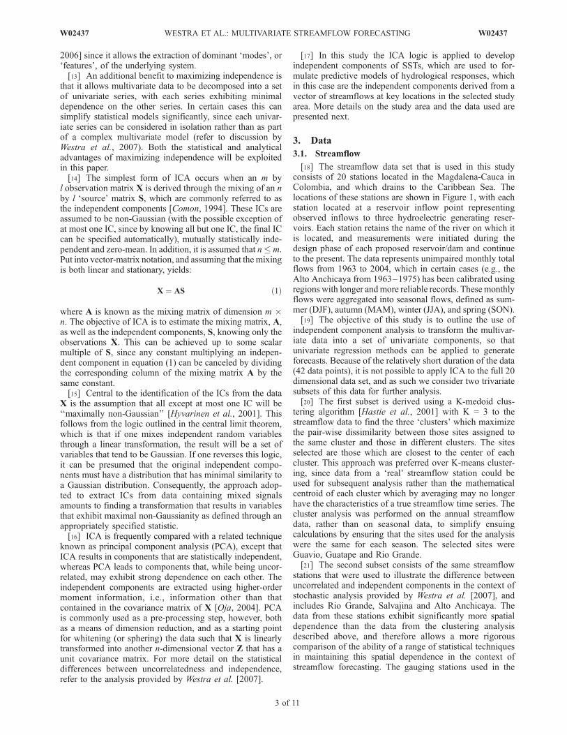
2006] since it allows the extraction of dominant ‘modes’, or‘features’, of the underlying system.[13] An additional benefit to maximizing independence is

that it allows multivariate data to be decomposed into a setof univariate series, with each series exhibiting minimaldependence on the other series. In certain cases this cansimplify statistical models significantly, since each univar-iate series can be considered in isolation rather than as partof a complex multivariate model (refer to discussion byWestra et al., 2007). Both the statistical and analyticaladvantages of maximizing independence will be exploitedin this paper.[14] The simplest form of ICA occurs when an m by

l observation matrix X is derived through the mixing of an nby l ‘source’ matrix S, which are commonly referred to asthe independent components [Comon, 1994]. These ICs areassumed to be non-Gaussian (with the possible exception ofat most one IC, since by knowing all but one IC, the final ICcan be specified automatically), mutually statistically inde-pendent and zero-mean. In addition, it is assumed that n�m.Put into vector-matrix notation, and assuming that the mixingis both linear and stationary, yields:

X ¼ AS ð1Þ

where A is known as the mixing matrix of dimension m �n. The objective of ICA is to estimate the mixing matrix, A,as well as the independent components, S, knowing only theobservations X. This can be achieved up to some scalarmultiple of S, since any constant multiplying an indepen-dent component in equation (1) can be canceled by dividingthe corresponding column of the mixing matrix A by thesame constant.[15] Central to the identification of the ICs from the data

X is the assumption that all except at most one IC will be‘‘maximally non-Gaussian’’ [Hyvarinen et al., 2001]. Thisfollows from the logic outlined in the central limit theorem,which is that if one mixes independent random variablesthrough a linear transformation, the result will be a set ofvariables that tend to be Gaussian. If one reverses this logic,it can be presumed that the original independent compo-nents must have a distribution that has minimal similarity toa Gaussian distribution. Consequently, the approach adop-ted to extract ICs from data containing mixed signalsamounts to finding a transformation that results in variablesthat exhibit maximal non-Gaussianity as defined through anappropriately specified statistic.[16] ICA is frequently compared with a related technique

known as principal component analysis (PCA), except thatICA results in components that are statistically independent,whereas PCA leads to components that, while being uncor-related, may exhibit strong dependence on each other. Theindependent components are extracted using higher-ordermoment information, i.e., information other than thatcontained in the covariance matrix of X [Oja, 2004]. PCAis commonly used as a pre-processing step, however, bothas a means of dimension reduction, and as a starting pointfor whitening (or sphering) the data such that X is linearlytransformed into another n-dimensional vector Z that has aunit covariance matrix. For more detail on the statisticaldifferences between uncorrelatedness and independence,refer to the analysis provided by Westra et al. [2007].

[17] In this study the ICA logic is applied to developindependent components of SSTs, which are used to for-mulate predictive models of hydrological responses, whichin this case are the independent components derived from avector of streamflows at key locations in the selected studyarea. More details on the study area and the data used arepresented next.

3. Data

3.1. Streamflow

[18] The streamflow data set that is used in this studyconsists of 20 stations located in the Magdalena-Cauca inColombia, and which drains to the Caribbean Sea. Thelocations of these stations are shown in Figure 1, with eachstation located at a reservoir inflow point representingobserved inflows to three hydroelectric generating reser-voirs. Each station retains the name of the river on which itis located, and measurements were initiated during thedesign phase of each proposed reservoir/dam and continueto the present. The data represents unimpaired monthly totalflows from 1963 to 2004, which in certain cases (e.g., theAlto Anchicaya from 1963–1975) has been calibrated usingregions with longer andmore reliable records. These monthlyflows were aggregated into seasonal flows, defined as sum-mer (DJF), autumn (MAM), winter (JJA), and spring (SON).[19] The objective of this study is to outline the use of

independent component analysis to transform the multivar-iate data into a set of univariate components, so thatunivariate regression methods can be applied to generateforecasts. Because of the relatively short duration of the data(42 data points), it is not possible to apply ICA to the full 20dimensional data set, and as such we consider two trivariatesubsets of this data for further analysis.[20] The first subset is derived using a K-medoid clus-

tering algorithm [Hastie et al., 2001] with K = 3 to thestreamflow data to find the three ‘clusters’ which maximizethe pair-wise dissimilarity between those sites assigned tothe same cluster and those in different clusters. The sitesselected are those which are closest to the center of eachcluster. This approach was preferred over K-means cluster-ing, since data from a ‘real’ streamflow station could beused for subsequent analysis rather than the mathematicalcentroid of each cluster which by averaging may no longerhave the characteristics of a true streamflow time series. Thecluster analysis was performed on the annual streamflowdata, rather than on seasonal data, to simplify ensuingcalculations by ensuring that the sites used for the analysiswere the same for each season. The selected sites wereGuavio, Guatape and Rio Grande.[21] The second subset consists of the same streamflow

stations that were used to illustrate the difference betweenuncorrelated and independent components in the context ofstochastic analysis provided by Westra et al. [2007], andincludes Rio Grande, Salvajina and Alto Anchicaya. Thedata from these stations exhibit significantly more spatialdependence than the data from the clustering analysisdescribed above, and therefore allows a more rigorouscomparison of the ability of a range of statistical techniquesin maintaining this spatial dependence in the context ofstreamflow forecasting. The gauging stations used in the

W02437 WESTRA ET AL.: MULTIVARIATE STREAMFLOW FORECASTING

3 of 11

W02437

analysis, including seasonal and annual mean streamflowsat each stations, are provided in Table 1.

3.2. Climate

[22] A global sea surface temperature anomaly (SSTA)data set was obtained from a reconstruction of raw SSTvalues using an optimal smoother, as described in [Kaplanet al., 1998]. On the basis of a simple correlation analysisbetween individual streamflow time series and the globaldata set (results not shown), it was found that statisticallysignificant correlations were found for certain stations andcertain seasons in all major oceans and for the full range of

latitudes. As a result, we decided not to reduce the globaldata set to a smaller geographic range. The linear trend ofabout 0.6 degrees Celsius was removed from each SSTAtime series before continuing with the analysis.[23] An index of the oceanic component of the ENSO

phenomenon, Nino 3.4, was also used in this analysis, andis defined as the seasonally averaged SSTA over the easternPacific [5�S – 5�N, 120�W – 170�W; Trenberth, 1997].Both the global SSTA data set and the Nino 3.4 index wereobtained from the International Research Institute for Cli-mate and Society (IRI) website (http://iri.columbia.edu). Ineach case, the data was aggregated to form seasonal time

Table 1. List of Gauging Stations Used in the Analysis, Together With Seasonal and Annual Mean Streamflow

(m3/s)a

Station Record DJF MAM JJA SON Annual

Guavio 1963–2004 70.2 (22.9) 201.7 (53.77) 399.5 (75.6) 192.8 (32.5) 864 (121)Guatape 1959–2004 74.4 (22.3) 97.9 (26.8) 88.9 (21.0) 130.9 (27.4) 392 (74)Rio Grande 1942–2004 78.7 (22.9) 95.8 (27.6) 100.9 (26.7) 126.6 (30.0) 402 (85)Salvajina 1947–2004 512.2 (194.6) 436.1 (126.7) 298.6 (51.1) 370.3 (115.3) 1617 (357)Alto Anchicaya 1963–2004 130.5 (29.5) 139.8 (28.6) 105.6 (26.8) 160.9 (28.4) 537 (78)

aStandard deviations are presented in parentheses.

Figure 1. Streamflow stations used in the analysis.

4 of 11

W02437 WESTRA ET AL.: MULTIVARIATE STREAMFLOW FORECASTING W02437

series. For the subsequent statistical model, concurrent datawas used throughout the analysis.

4. Methodology

4.1. Forecasting Overview

[24] The objective of this paper is to describe variousmethods to forecast seasonal streamflow for a water supplycatchment in Colombia, and demonstrate certain benefits informulating the forecasting models by considering indepen-dence in both predictor and predictand data sets. Each of theforecasting approaches will be applied to both subsets ofthree streamflow stations identified in section 3.[25] Let the trivariate streamflow data be represented by

Xq,t = {xq,1,t, xq,2,t, xq,3,t}. The subscript, q, will be usedthroughout this paper to indicate a streamflow variable,whereas the subscript, s, will be used to refer to the SSTdata set. All streamflow data has been normalized bysubtracting the seasonal mean and dividing by the standarddeviation, and as such represents seasonal anomaly data.Note that each xq,i,t represents a time series for a particularseason, with the season denoted by t. Arguably the mostsimple forecast model is to consider the previous seasonstreamflow time series (t-1) in an autoregressive order-1model, as described below:

xq;i;t ¼ bAR;txq;t�1 þ e 1ð Þi;t ð2Þ

where bAR,t represents the regression coefficient for thatseason for the autoregressive model, and i2{1, 2, 3} repre-sents individual streamflow time series, such that a separatemodel is developed for each streamflow station. The previousseason streamflow, represented by xq,t-1 is taken as theunweighted average streamflow from each of the threestations, and therefore does not contain the subscript i. Thiswas preferred over using a separate predictor (i.e., streamflowfor the previous season at the same site) for eachmodel, in theinterest of keeping the modeling structure as parsimonious aspossible, and also because of the spatial linkages the respec-tive flows have with each other.[26] The approach represented by equation 2 is equivalent

to the standard climatology plus persistence model, and asdiscussed in the Introduction of this paper, any forecastmodel should be tested against this basic model to determinewhether using exogenous variables relating to a climate statewill result in an increase in predictability. As a result, theremainder of this paper will focus on improving this basicmodel by focusing on minimizing the error component, ei,t

(1).Four such approaches will be considered, including:[27] 1) Considering an index of the ENSO phenomenon,

Nino 3.4, as the predictor, and regressing this predictoragainst the error ei,t

(1) associated with each univariate stream-flow time series individually;[28] 2) Using ICA on the SSTA data to obtain a multivar-

iate SSTA predictor field, which will be regressed againsteach univariate streamflow error time series ei,t

(1) individually;[29] 3) Applying CCA to model both multivariate pre-

dictor and multivariate predictand, by using eigen-decom-position techniques to maintain second order dependenciesin the data; and[30] 3) Applying ICA to both the multivariate predictor

and multivariate predictand, using an information-theoretic

approach to maintain second- and higher-order dependen-cies in the data.[31] Note that both the Nino 3.4 index and the SSTA data

used for the forecasts are concurrent, to simplify theanalysis. In reality, of course, the user will not have accessto concurrent information to develop future projections, andas such, this method will need to be modified to incorporatea forecasting model for SSTAs (using either statistical ordynamical means), or alternatively using a lagged relation-ship between predictor and predictand.

4.2. Approach 1 - Regression of the Nino 3.4Index Against Univariate Streamflow Residuals

[32] We present first a simple regression model that usesthe Nino 3.4 index as a measure of the oceanic componentof ENSO variability:

xq;i;t ¼ bARxq;t�1 þ bNINO34zt þ e 2ð Þi;t ð3Þ

where zt represents the seasonal Nino 3.4 index at season t,and bNINO34 represents the regression coefficient for thispredictor. This model is mathematically and computation-ally simple, and is frequently also highly interpretable, sincea statistically significant model will demonstrate a directrelationship between the hydrological variable of interest,and a known measure of exogenous climate variability. Itsmain disadvantages is that each streamflow time series ismodeled independently, and hence cannot be expected toexhibit the spatial dependence one would observe in thehistorical data. An additional disadvantage is the reliance onENSO as the only mode of variability, a strong assumptiongiven evidence of secondary effects that change streamflowpatterns around the world.

4.3. Approach 2 - Regression of Multivariate SSTAsAgainst Univariate Streamflow Residuals

[33] Our second model includes sea surface temperatureanomalies as an additional factor in predicting flows,consistent with the recommendations of [Paegle and Mo,2002]. This is done by first applying PCA to reduce thedimension of the global SSTA data set, followed byapplication of ICA to the retained components to enhancethe interpretability of each component. We considered sixcomponents in total, which is based on a compromisebetween maximizing interpretability of individual ICs whileat the same time maximizing the variance explained in theoriginal data set. This allows two predictors on average foreach of the three predictands. The ensuing model is writtenas follows:

xq;i;t ¼ bARxq;t�1 þXj

bjys;j;t þ e 3ð Þi;t ð4Þ

where ys,j,t represents estimates of the independent compo-nents, S, obtained by applying equation (1) to the SSTAdata set for season t. Here, j2{1, 2, . . ., 6} represents thesubset of predictors obtained from the set of independentcomponents from the SSTA data set, selected using aforward stepwise selection procedure with the partialt-statistic for testing whether a predictor should be included.We use a 90 percentile cut-off t value of 1.68 whichcorresponds to a correlation coefficient of 0.255. It was

W02437 WESTRA ET AL.: MULTIVARIATE STREAMFLOW FORECASTING

5 of 11

W02437

found that a large number of predictors were excluded usingthe slightly higher 95 percentile t value, which we believe ispartly due to the difficultly in demonstrating statisticalsignificance for such short data sets, particularly whenlooking beyond the first predictor, which is usually relatedto the ENSO phenomenon. It should be noted that thismodel would be expected to reflect variability due to abroader set of causes than just ENSO, but would still beconstrained in its representation of spatial dependenceacross the streamflow variables being modeled.

4.4. Approach 3 - Use of Canonical CorrelationAnalysis to Relate the Multivariate SSTAs toMultivariate Streamflow

[34] The disadvantage of the above two methods in thepresent context is that a separate model is formulated for eachof the streamflow time series, without any provision to ensurean accurate representation of the spatial dependence thatexists across the streamflow variable vector. A widely usedapproach for incorporating spatial dependence is known ascanonical correlation analysis (CCA), which is a mathemat-ical approach for identifying pairs of patterns in two multi-variate data sets, and constructing sets of transformedvariables by projecting the original data onto these patterns[Wilks, 2006]. For the purposes of this study, the predictorsand predictands are the global SST data set represented byXs,t, and the trivariate reservoir inflow data set after account-ing for persistence represented by Et

(1), respectively.[35] The following is a brief overview of CCA, based on

the discussion by Wilks [2006] but with notation adjusted tobe consistent with notation used elsewhere in this paper.[36] The aim of CCA is to transform the original (cen-

tered) multivariate data sets Xs,t and Et(1) into a set of

canonical variates, V and W, defined by:

V ¼ ATXs;t ð5Þ

W ¼ BTE1ð Þt ð6Þ

The vectors of weights, A and B, are the canonical vectors,which are obtained through an eigen-decomposition of Xs,t

and Et(1), with further details provided by Wilks [2006]. This

results in the canonical variates having the properties

Corr Vi;Wn½ ¼ rCi; i ¼ n

0; i 6¼ n

�ð7Þ

where rCi is obtained through an eigen decomposition of thejoint predictand-predictor covaiances matrices. Since the rCiallows each element of V to be related to a unique elementof W, estimation of W can be accomplished through thefollowing linear relationship:

W ¼ RC½ V ð8Þ

where

RC½ ¼

rC1 0 0

0 rC2 0

0 0 rC3

266664

377775 ð9Þ

Using W, it is possible to develop an estimate of Et(1) through

the inverse of equation (6), which completes the specificationof the CCA based forecasting procedure used in our study.

4.5. Approach 4 - Regression of MultivariateSSTAs Against Multivariate Streamflow Residuals

[37] Finally, we present an alternative approach thatfollows on from the multivariate resampling logic presentedby Westra et al. [2007], which is based on transforming themultivariate predictor and predictand into a set of univariateseries which do not exhibit dependence on each other. TheICA-based approach was compared with a PCA-basedapproach by Westra et al. [2007], and it was found thatby focusing on statistical independence rather than correla-tion, ICA better represented spatial dependence of themultivariate data.[38] A similar advantage is expected in this paper, where

CCA considers only the information contained in thecovariance matrix (second order statistics), whereas ICAprovides an additional rotation to maximize some measureof statistical dependence. The forecasting approach adoptedin this paper is presented below, and further details on thestatistical properties of ICA are given by Hyvarinen et al.[2001] and Westra et al. [2007].[39] We start by transforming the error term in equation

(2) to yield:

Yq eð Þ;t ¼ Wq eð Þ;tE1ð Þt ð10Þ

This equation is analogous to the inverse form of equation(1), where Yq(e)t represents an estimate of a set ofindependent components, Et

(1) represents the original mixedmultidimensional error matrix from equation (2) and Wrepresents an estimate of the inverse of the mixing matrix,A. Note we use bold to represent the full multivariate data,and as such the subscript i is not included.[40] Since Yq(e),t consists of a set of independent compo-

nents, it can be factorized into yq(e),i,t, with i2 {1, 2, 3},without loss of information. This allows for individualyq(e),i,t to be related to selected independent componentsof the multivariate SSTA data as was done in the previousapproach. This gives us the following model:

yq eð Þ;i;t ¼Xj

bjys;j;t þ e 4ð Þi;t ð11Þ

with each variable defined as before. Because the yq(e),i,t’sare mutually independent, it is possible to generate theforecasting model without distorting the spatial dependencestructure inherent in the original data. To achieve this,however, a modification to the forward selection processused in section 4.3 is necessary, to ensure that differentyq(e),i,t’s do not end up with the same predictor. This isachieved as follows:[41] 1) Start by sorting the yq(e),i,t’s by variance explained,

with yq(e),1,t representing the maximum variance, and yq(e),3,trepresenting the minimum variance;[42] 2) For yq(e),1,t, find the SST independent component

ys,j,t that yields the maximum correlation coefficient. If thisis higher than the 90 percentile t statistic cut-off of 1.68,retain this as a predictor of yq(e),1,t, and remove from thepool of available predictors;

6 of 11

W02437 WESTRA ET AL.: MULTIVARIATE STREAMFLOW FORECASTING W02437

[43] 3) Repeat step (2) for yq(e),2,t and yq(e),3,t, so that eachyq(e),i,t has at most one predictor;[44] 4) Repeat steps (2) and (3) to add a second predictor

for each case where the t statistic is higher than the cut-offvalue of 1.68. Each time a predictor is added to the model, itshould be removed from the pool of available predictors sothat a given predictor can not be selected twice.[45] We now have a model for each streamflow IC,

consisting of at most two predictors. Using this model, wecan estimate yq(e),i,t for all i, followed by a rotation intooriginal space using the equation:

e 1ð Þt ¼ W�1

q eð Þ;t yq eð Þ;t ð12Þ

Where W�1 represents the inverse of W.[46] The final estimates of streamflow can now be written

as:

xq;i;t ¼ bARxq;t�1 þ e1ð Þi;t ð13Þ

We now have four alternative forecasting approaches, aswell as a baseline persistence model, which we wish tocompare both in terms of forecast performance forindividual streamflow stations, and the ability to capturethe spatial dependence of the multivariate data. Thiscomparison is the subject of the following section.

5. Results

5.1. Spearman’s Correlation as a Measure ofModel Accuracy

[47] The objective of a forecast model is to make projec-tions of a given predictand forward in time. The way our

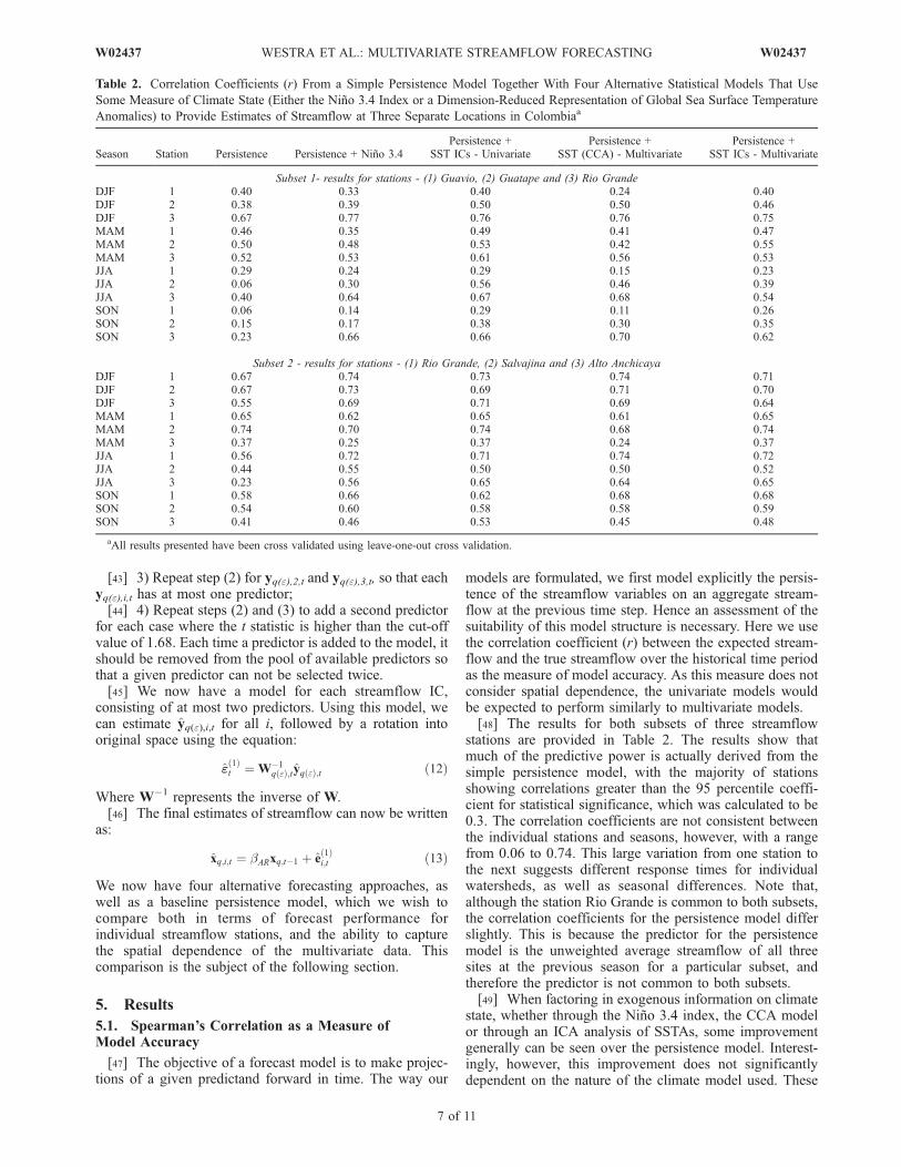
models are formulated, we first model explicitly the persis-tence of the streamflow variables on an aggregate stream-flow at the previous time step. Hence an assessment of thesuitability of this model structure is necessary. Here we usethe correlation coefficient (r) between the expected stream-flow and the true streamflow over the historical time periodas the measure of model accuracy. As this measure does notconsider spatial dependence, the univariate models wouldbe expected to perform similarly to multivariate models.[48] The results for both subsets of three streamflow

stations are provided in Table 2. The results show thatmuch of the predictive power is actually derived from thesimple persistence model, with the majority of stationsshowing correlations greater than the 95 percentile coeffi-cient for statistical significance, which was calculated to be0.3. The correlation coefficients are not consistent betweenthe individual stations and seasons, however, with a rangefrom 0.06 to 0.74. This large variation from one station tothe next suggests different response times for individualwatersheds, as well as seasonal differences. Note that,although the station Rio Grande is common to both subsets,the correlation coefficients for the persistence model differslightly. This is because the predictor for the persistencemodel is the unweighted average streamflow of all threesites at the previous season for a particular subset, andtherefore the predictor is not common to both subsets.[49] When factoring in exogenous information on climate

state, whether through the Nino 3.4 index, the CCA modelor through an ICA analysis of SSTAs, some improvementgenerally can be seen over the persistence model. Interest-ingly, however, this improvement does not significantlydependent on the nature of the climate model used. These

Table 2. Correlation Coefficients (r) From a Simple Persistence Model Together With Four Alternative Statistical Models That Use

Some Measure of Climate State (Either the Nino 3.4 Index or a Dimension-Reduced Representation of Global Sea Surface Temperature

Anomalies) to Provide Estimates of Streamflow at Three Separate Locations in Colombiaa

Season Station Persistence Persistence + Nino 3.4Persistence +

SST ICs - UnivariatePersistence +

SST (CCA) - MultivariatePersistence +

SST ICs - Multivariate

Subset 1- results for stations - (1) Guavio, (2) Guatape and (3) Rio GrandeDJF 1 0.40 0.33 0.40 0.24 0.40DJF 2 0.38 0.39 0.50 0.50 0.46DJF 3 0.67 0.77 0.76 0.76 0.75MAM 1 0.46 0.35 0.49 0.41 0.47MAM 2 0.50 0.48 0.53 0.42 0.55MAM 3 0.52 0.53 0.61 0.56 0.53JJA 1 0.29 0.24 0.29 0.15 0.23JJA 2 0.06 0.30 0.56 0.46 0.39JJA 3 0.40 0.64 0.67 0.68 0.54SON 1 0.06 0.14 0.29 0.11 0.26SON 2 0.15 0.17 0.38 0.30 0.35SON 3 0.23 0.66 0.66 0.70 0.62

Subset 2 - results for stations - (1) Rio Grande, (2) Salvajina and (3) Alto AnchicayaDJF 1 0.67 0.74 0.73 0.74 0.71DJF 2 0.67 0.73 0.69 0.71 0.70DJF 3 0.55 0.69 0.71 0.69 0.64MAM 1 0.65 0.62 0.65 0.61 0.65MAM 2 0.74 0.70 0.74 0.68 0.74MAM 3 0.37 0.25 0.37 0.24 0.37JJA 1 0.56 0.72 0.71 0.74 0.72JJA 2 0.44 0.55 0.50 0.50 0.52JJA 3 0.23 0.56 0.65 0.64 0.65SON 1 0.58 0.66 0.62 0.68 0.68SON 2 0.54 0.60 0.58 0.58 0.59SON 3 0.41 0.46 0.53 0.45 0.48

aAll results presented have been cross validated using leave-one-out cross validation.

W02437 WESTRA ET AL.: MULTIVARIATE STREAMFLOW FORECASTING

7 of 11

W02437

results suggest that the streamflow time series analyzed hereare largely persistence + ENSO driven, with little additionalinformation derived from considering other regions ofoceanic variability. Finally, it is noted that the differentparameterizations of each modeling approach wereaccounted for by using leave-one-out cross validation ingenerating all the model results.[50] To provide a visual assessment of the performance of

the multivariate ICA model, the results of this model arecompared with actual recorded winter inflows for each ofthe stations in Subset 2, and have been plotted in Figure 2.The recorded inflows are plotted as a blue line, with the bestestimates from the multivariate ICA model presented as asolid red line. The correlation coefficients between recordedand estimated inflows for Rio Grande, Salvajina and AltoAnchicaya are 0.72, 0.52, and 0.65, respectively. The 5%and 95% confidence levels are plotted as dashed red lines,and are generated through bootstrapping the error terms foreach approach and taking the 5th and 95th percentile foreach estimate.[51] The main result from this analysis is therefore that no

significant improvement can be observed for the morecomplex persistence + SSTA ICs models compared withthe more parsimonious persistence + Nino 3.4 model, so

that from a univariate forecasting perspective there is astrong case in favor of choosing the simpler model toforecast streamflow. Similarly, however, there is no evi-dence of any loss in predictive power using the multivariatepersistence + SSTA ICs model compared with the suite ofother approaches analyzed, since this model performsequally well on a temporal basis compared to the univariatemodels. As such, the key question is how ICA representsthe spatial dependence, and this is discussed further in thesection below.

5.2. Spatial Dependence

[52] The main benefit of the multivariate ICA approach isits ability to capture the spatial dependence of the multi-variate streamflow time series, and this can be explored onlyusing a multivariate dependence measure. One such mea-sure is the mean integrated squared bias (MISB), which isevaluated as follows [Scott, 1992]:

Zf � f �

dXq;t

ð14Þ

where F is the kernel density estimate [see Sharma, 2000b;Westra et al., 2007, for details] of the original multivariate

Figure 2. Time series of historical flows (blue line) and estimated flows based on multivariate ICAregression model (red solid line), for Rio Grande (top), Salvajina (middle) and Alto Anchicaya (bottom).Dotted red lines represent 5% and 95% significance levels.

8 of 11

W02437 WESTRA ET AL.: MULTIVARIATE STREAMFLOW FORECASTING W02437

data, Xq,t, which is taken to be the true density, and frepresents the kernel density estimate of the forecast data,Xq,t. The MISB is calculated using trivariate kernel densityestimates to evaluate the joint dependence structure, and theresults for each season and for each of the four models areprovided in Table 3.[53] Note that, to generate Xq,t in this case we bootstrap

the error terms in each approach to generate multipleplausible realizations of the forecasts. This enables theprovision of forecasts in a probabilistic setting, so that therange of likely outcomes can be taken into account.The results in this section are based on 5000 such proba-bilistic forecasts of the streamflow variables being modeled.[54] The results from Table 3 demonstrate that, in general,

the univariate models (i.e., the persistence-only, the persis-tence + Nino 3.4 and the univariate persistence + SST ICsmodels) tend to perform similarly to each other, and have ahigher MISB (i.e., poorer representation of spatial depen-dence) compared with the multivariate models. This differ-ence is particularly notable for the second trivariate subsetcontaining the stations Rio Grande, Salvajina and AltoAnchicaya, since the spatial correlation of the original datais greater than for the first trivariate subset. In contrast, thefirst subset, containing the stations Guavio, Guatape andRio Grande, does not exhibit a great amount of spatialdependence, largely due to the clustering algorithm used toobtain the stations since this algorithm seeks stations thatexhibit maximal within-cluster dependence while at thesame time minimizing between-cluster dependence.[55] Considering the multivariate models, it can be seen

that although the CCA-based approach results in a signif-icant improvement in the MISB score over the univariateapproaches, the best results are reserved for the multivariateICA approach, since this approach explicitly considers thefull joint dependence in the data. The average percentageimprovement in MISB score using the ICA-based approachfor subsets 1 and 2 was 14% and 22%, respectively.[56] As discussed earlier, the logic for the difference in

results between the CCA- and ICA-based forecasting mod-els is equivalent to the PCA- and ICA-based stochasticgeneration models compared byWestra et al. [2007]; that is,by considering the full dependence structure in a multivar-iate data set rather than focus on covariance or correlation-based statistics alone, it is possible to better simulate thejoint probability density of the data. In this earlier paper,rather than consider two trivariate subsets, 992 trivariate

combinations from the Colombia reservoir inflow data setwere simulated, with the results showing an average im-provement in the MISB score of 25% for the ICA-basedapproach. Although computational considerations precludesuch a detailed analysis for the present study, the results forthe two subsets considered here are consistent with theseearlier results.[57] Finally to illustrate the results from Table 3, we

consider the performance of winter streamflow for thesecond subset, with joint dependence results presented inFigure 3. Only the CCA and ICA results are considered,since these are the only models that explicitly considerspatial dependence. The point to note is the smoothening inthe multivariate results from both CCA and ICA in com-parison to the raw data, which is to be expected because ofthe use of the bootstrapping procedure. While differences inthe CCA and ICA results are not visually apparent, MISBcalculations for the two indicate an improved representationof spatial dependence in the ICA model, as illustrated inTable 3.

6. Conclusions

[58] The objective of this paper is to demonstrate thatgeneration of probabilistic multivariate seasonal streamflowforecasts using independent component analysis containssignificant advantages over a range of alternative modelsthat are commonly used. These alternative models include asimple persistence-only model, a persistence + Nino 3.4model, a univariate persistence + SST ICs model and amultivariate CCA model. The results were evaluated both interms of the ability to forecast seasonal streamflow, as wellas whether the models were able to maintain the spatialvariability that is present in the original data.[59] When examining temporal dependence, with the

exception of the persistence-only model, all other modelsperform comparably in terms of the correlation coefficientbetween true streamflow and estimated streamflow, suggest-ing that most of the variability in Colombia streamflow is aresult of ENSO-driven processes. In contrast, a dramaticimprovement can be seen between the multivariate ICAmodel compared with all the univariate models in terms ofmaintaining spatial dependence, and this improvementbecomes more pronounced as the spatial proximity orclimatological similarity between the stations is increased.

Table 3. Mean Integrated Squared Bias (MISB) Results Comparing the Multivariate (Three Dimensional) Kernel Density Estimates of

the Predicted Data Against the Three-Dimensional Kernel Density Estimates of the Original Dataa

Season Persistence Persistence + Nino 3.4Persistence +

SST ICs - UnivariatePersistence +

SST (CCA) - MultivariatePersistence +

SST ICs - Multivariate

Subset 1: Results for stations - Guavio, Guatape and Rio GrandeDJF 0.0068 0.0069 0.0069 0.0061 0.0059MAM 0.0056 0.0059 0.0058 0.0048 0.0042JJA 0.0031 0.0032 0.0030 0.0022 0.0018SON 0.0063 0.0059 0.0066 0.0037 0.0029

Subset 2: Results for stations - Rio Grande, Salvajina and Alto AnchicayaDJF 0.0700 0.0723 0.0713 0.0371 0.0299MAM 0.0140 0.0162 0.0141 0.0089 0.0058JJA 0.0097 0.0096 0.0071 0.0062 0.0051SON 0.0159 0.0178 0.0179 0.0113 0.0094

aThe MISB has been calculated for each streamflow model for four seasons, after cross-validation.

W02437 WESTRA ET AL.: MULTIVARIATE STREAMFLOW FORECASTING

9 of 11

W02437

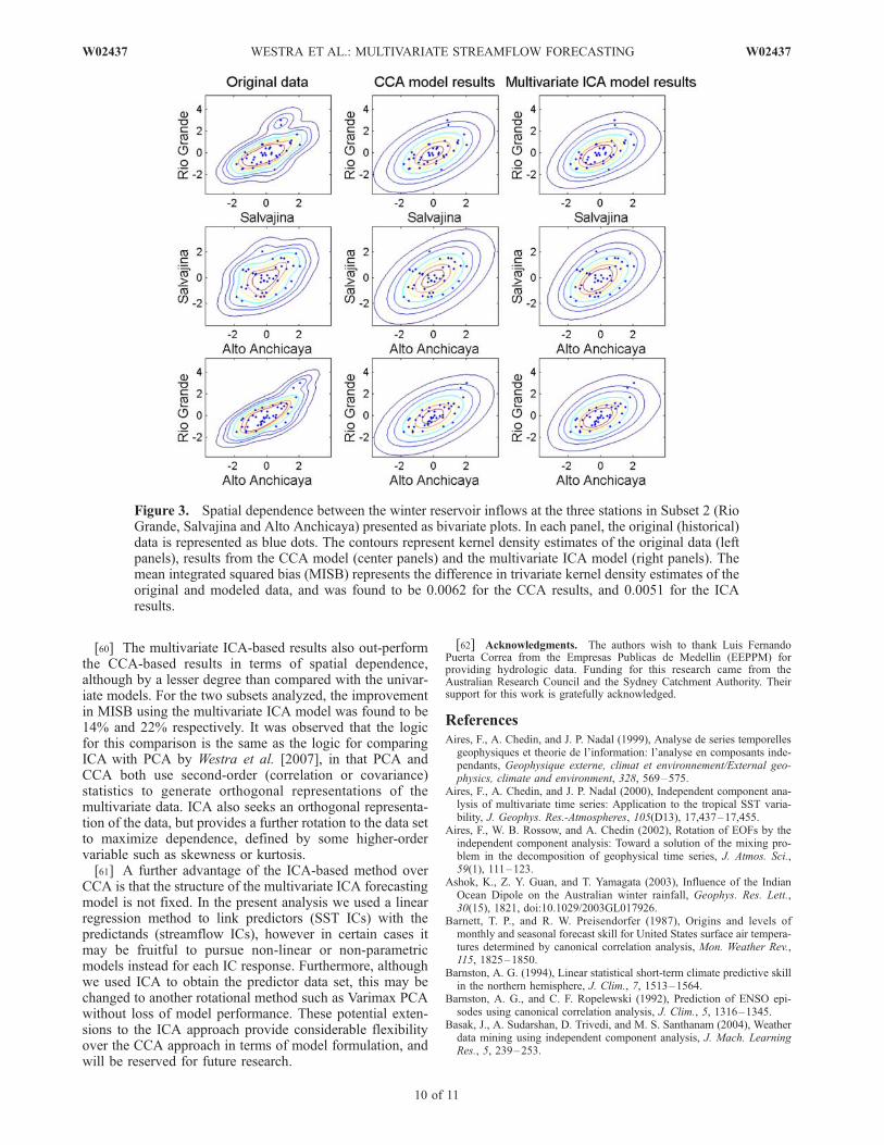
[60] The multivariate ICA-based results also out-performthe CCA-based results in terms of spatial dependence,although by a lesser degree than compared with the univar-iate models. For the two subsets analyzed, the improvementin MISB using the multivariate ICA model was found to be14% and 22% respectively. It was observed that the logicfor this comparison is the same as the logic for comparingICA with PCA by Westra et al. [2007], in that PCA andCCA both use second-order (correlation or covariance)statistics to generate orthogonal representations of themultivariate data. ICA also seeks an orthogonal representa-tion of the data, but provides a further rotation to the data setto maximize dependence, defined by some higher-ordervariable such as skewness or kurtosis.[61] A further advantage of the ICA-based method over

CCA is that the structure of the multivariate ICA forecastingmodel is not fixed. In the present analysis we used a linearregression method to link predictors (SST ICs) with thepredictands (streamflow ICs), however in certain cases itmay be fruitful to pursue non-linear or non-parametricmodels instead for each IC response. Furthermore, althoughwe used ICA to obtain the predictor data set, this may bechanged to another rotational method such as Varimax PCAwithout loss of model performance. These potential exten-sions to the ICA approach provide considerable flexibilityover the CCA approach in terms of model formulation, andwill be reserved for future research.

[62] Acknowledgments. The authors wish to thank Luis FernandoPuerta Correa from the Empresas Publicas de Medellin (EEPPM) forproviding hydrologic data. Funding for this research came from theAustralian Research Council and the Sydney Catchment Authority. Theirsupport for this work is gratefully acknowledged.

ReferencesAires, F., A. Chedin, and J. P. Nadal (1999), Analyse de series temporellesgeophysiques et theorie de l’information: l’analyse en composants inde-pendants, Geophysique externe, climat et environnement/External geo-physics, climate and environment, 328, 569–575.

Aires, F., A. Chedin, and J. P. Nadal (2000), Independent component ana-lysis of multivariate time series: Application to the tropical SST varia-bility, J. Geophys. Res.-Atmospheres, 105(D13), 17,437–17,455.

Aires, F., W. B. Rossow, and A. Chedin (2002), Rotation of EOFs by theindependent component analysis: Toward a solution of the mixing pro-blem in the decomposition of geophysical time series, J. Atmos. Sci.,59(1), 111–123.

Ashok, K., Z. Y. Guan, and T. Yamagata (2003), Influence of the IndianOcean Dipole on the Australian winter rainfall, Geophys. Res. Lett.,30(15), 1821, doi:10.1029/2003GL017926.

Barnett, T. P., and R. W. Preisendorfer (1987), Origins and levels ofmonthly and seasonal forecast skill for United States surface air tempera-tures determined by canonical correlation analysis, Mon. Weather Rev.,115, 1825–1850.

Barnston, A. G. (1994), Linear statistical short-term climate predictive skillin the northern hemisphere, J. Clim., 7, 1513–1564.

Barnston, A. G., and C. F. Ropelewski (1992), Prediction of ENSO epi-sodes using canonical correlation analysis, J. Clim., 5, 1316–1345.

Basak, J., A. Sudarshan, D. Trivedi, and M. S. Santhanam (2004), Weatherdata mining using independent component analysis, J. Mach. LearningRes., 5, 239–253.

Figure 3. Spatial dependence between the winter reservoir inflows at the three stations in Subset 2 (RioGrande, Salvajina and Alto Anchicaya) presented as bivariate plots. In each panel, the original (historical)data is represented as blue dots. The contours represent kernel density estimates of the original data (leftpanels), results from the CCA model (center panels) and the multivariate ICA model (right panels). Themean integrated squared bias (MISB) represents the difference in trivariate kernel density estimates of theoriginal and modeled data, and was found to be 0.0062 for the CCA results, and 0.0051 for the ICAresults.

10 of 11

W02437 WESTRA ET AL.: MULTIVARIATE STREAMFLOW FORECASTING W02437

Casey, T. M. (1998), Assessment of a seasonal forecast model, Aust. Me-teorol. Mag., 47, 103–111.

Chiew, F. H. S., and T. A. McMahon (2002), Modelling the impacts ofclimate change on Australian streamflow, Hydrol. Processes, 16(6),1235–1245.

Comon, P. (1994), Independent component analysis: A new concept?, Sig-nal Processing, 36, 287–314.

Drosdowsky, W., and L. E. Chambers (2001), Near-global sea surfacetemperature anomalies as predictors of Australian seasonal rainfall,J. Clim., 14, 1677–1687.

Filho, F. A. S., and U. Lall (2003), Seasonal to interannual ensemblestreamflow forecasts for Ceara, Brazil: Applications of a multivariate,semiparametric algorithm, Water Resour. Res., 39(11), 1307,doi:10.1029/2002WR001373.

Goddard, L., et al. (2001), Current approaches to seasonal-to-interannualclimate predictions, Int. J. Climatol., 21(9), 1111–1152.

Hamlet, A. F., D. Huppert, and D. P. Lettenmaier (2002), Economic valueof long-lead streamflow forecasts for Columbia river hydropower,J. Water Resour. Plann. Manage., 128, 91–101.

Hastie, T., R. Tibshirani, and J. Friedman (2001), The Elements of Statis-tical Learning: Data Mining, Inference and Prediction. Springer Seriesin Statistics, Springer, New York, 553 pp.

Herault, J., and C. Jutten (1986), Space or time adaptive signal processingby neural network models, in Neural networks for computing: AIP con-ference proceedings American Institute for physics, edited by J. S. Den-ker, New York.

Huang, J., H. M. Van Den Dool, and A. G. Barnston (1996), Long-leadseasonal temperature prediction using optimal climate normals, J. Clim.,9, 809–817.

Hurrell, J. W. (1995), Decadal trends in the North Atlantic Oscillation:Regional temperature and precipitation, Science, 269, 676–679.

Hurrell, J. W., and H. Van Loon (1997), Decadal variations in climateassociated with the NAO, Clim. Change, 36, 301–326.

Hwang, S. O., J. K. E. Schemm, A. G. Barnston, and W. T. Kwon (2001),Long-lead seasonal forecast skill in far eastern Asia using canonicalcorrelation analysis, J. Clim., 14, 3005–3016.

Hyvarinen, A. (1999), Survey on Independent Component Analysis, NeuralComput. Surv., 2, 94–128.

Hyvarinen, A., J. Karhunen, and E. Oja (2001), Independent ComponentAnalysis, John Wiley and Sons, New York, 481 pp.

Ilin, A., H. Valpola, and E. Oja (2006), Exploratory analysis of climate datausing source separation methods, Neural Networks, 19, 155–167.

Kaplan, A., et al. (1998), Analyses of global sea surface temperature 1856–1991, J. Geophys. Res. Oceans, 103(C9), 18,567–18,589.

Lee, T. W. (1998), Independent Component Analysis - Theory and Applica-tions, Kluwer Academic Publishers, Boston.

Mason, S. J., and L. Goddard (2001), Probabilistic precipitation anomaliesassociated with ENSO, Bull. Am. Meteorol. Soc., 82(4), 619–638.

McBride, J. L., and N. Nicholls (1983), Seasonal relationships betweenAustralian rainfall and the Southern Oscillation, Mon. Weather Rev.,11, 1998–2004.

Nicholls, N. (1989), Sea surface temperatures and Australian winter rain-fall, J. Clim., 2, 965–973.

Oja, E. (Ed.) (2004), Applications of Independent Component Analysis.Neural Information Processing - Lecture Notes in Computer Science,3316, Springer Berlin/Heidelberg, 1044–1051 pp.

Paegle, J. N., and K. C. Mo (2002), Linkages between summer rainfallvariability over South America and sea surface temperature anomalies,J. Clim., 15(12), 19.

Richman, M. B. (1986), Rotation of principal components, J. Climatol., 6,293–335.

Ropelewski, C. F., and M. S. Halpert (1996), Quantifying Southern Oscil-lation - Precipitation relationships, J. Clim., 9, 1043–1059.

Saji, N. H., and T. Yamagata (2003), Possible impacts of Indian OceanDipole mode events on global climate, Clim. Res., 25(2), 151–169.

Saji, N. H., B. N. Goswami, P. N. Vinayachandran, and T. Yamagata(1999), A dipole mode in the tropical Indian Ocean, Nature, 401,360–363.

Scott, D. W. (1992), Multivariate Density Estimation: Theory, Practice andVisualisation. Probability and Mathematical Statistics, John Wiley &Sons Inc., New York, 317 pp.

Shabbar, A., and A. G. Barnston (1996), Skill of seasonal climate forecastsin Canada using canonical correlation analysis, Mon. Weather Rev., 124,2370–2385.

Sharma, A. (2000a), Seasonal to interannual rainfall probabilistic forecastsfor improved water supply management: Part 1 - A strategy for systempredictor identification, J. Hydrol., 239, 232–239.

Sharma, A. (2000b), Seasonal to interannual rainfall probabilistic forecastsfor improved water supply management: Part 3 - A non-parametric prob-abilistic forecast model, J. Hydrol., 239, 249–258.

Singhrattna, N., B. Rajagopalan, M. Clark, and K. K. Kumar (2005), Sea-sonal forecasting of Thailand summer monsoon rainfall, Int. J. Climatol.,25, 649–664.

Stone, R. C., G. L. Hammer, and T. Marcussen (1996), Prediction of globalrainfall probabilities using phases of the Southern Oscillation Index,Nature, 384, 252–255.

Storch, H. v., and F. W. Zwiers (2001), Statistical Analysis in ClimateResearch, Cambridge University Press.

Trenberth, K. E. (1997), The definition of El Nino, Bull. Am. Meteorol.Soc., 78, 2,771–2,777.

Verdon, D. C., A. M. Wyatt, A. S. Kiem, and S. W. Franks (2004), Multi-decadal variability of rainfall and streamflow: Eastern Australia, WaterResour. Res., 40(10), W10201, doi:10.1029/2004WR003234.

Westra, S. P., C. Brown, U. Lall, and A. Sharma (2007), Modeling multi-variable hydrological series: Principal component analysis or indepen-dent component analysis?, Water Resour. Res., 43, W06429,doi:10.1029/2007WR005617.

Wilks, D. S. (2006), Statistical Methods in the Atmospheric Sciences. Inter-national Geophysics Series, Elsevier, Amsterdam.

Woolddridge, S. A., M. F. Hutchinson, and J. D. Kalma (1999), Interpola-tion of rainfall data from raingauges and radar using thin plate smoothingsplines, WATER99 Joint Congress. Institution of Engineers, Australia,Brisbane, Australia, pp. 263–268.

Yao, H., and A. Georgakakos (2001), Assessment of Folsom Lake responseto historical and potential future climate scenarios - 2. Reservoir manage-ment, J. Hydrol., 249, 176–196.

����������������������������C. Brown and U. Lall, Department of Earth and Environmental

Engineering, Columbia University, New York, NY 10027, USA. (caseyb@iri.columbia.edu; ula2@columbia.edu)

A. Sharma, School of Civil and Environmental Engineering, TheUniversity of New South Wales, Sydney, NSW 2052, Australia.(a.sharma@unsw.edu.au)

S. Westra, Sinclair Knight Merz, 100 Christie Street, St Leonards, NSW,Australia. (swestra@skm.com.au)

W02437 WESTRA ET AL.: MULTIVARIATE STREAMFLOW FORECASTING

11 of 11

W02437