Automatic Calibration of the SHETRAN HydrologicalModelling System Using MSCE

Rong Zhang & Celso A. G. Santos & Madalena Moreira & Paula K. M. M. Freire &

João Corte-Real

Received: 1 May 2012 /Accepted: 16 June 2013 /Published online: 26 June 2013# Springer Science+Business Media Dordrecht 2013

Abstract Automatic calibration is preferred because it provides an objective and extensivesearching in the feasible parameter space. In this study, the Modified Shuffled ComplexEvolution (MSCE) optimization algorithm is applied to automatically calibrate thephysically-based spatially-distributed hydrological model SHETRAN in the 705-km2

semi-arid Cobres basin in southern Portugal, with a spatial resolution of 2 km and a temporalresolution of 1 h. Twenty-two parameters are calibrated for the main types of land-use andsoil. Nash-Sutcliffe Efficiency (NSE) is 0.86 for calibration and 0.74 for validation for basinoutlet; NSE is respectively 0.65 and 0.82 for calibration, 0.69 and 0.63 for validation ofinternal gauging stations Albernoa and Entradas. As for storm events, NSE is 0.87 and 0.64respectively for Storms No.1 (during the calibration period) and No.4 (during the validationperiod) at basin outlet; it is 0.69 and 0.65 for Storm No.4 respectively at Albernoa and

Water Resour Manage (2013) 27:4053–4068DOI 10.1007/s11269-013-0395-z

R. Zhang (*) :M. Moreira : J. Corte-RealInstitute of Mediterranean Agrarian and Environmental Sciences (ICAAM), Group Water, Soil and Climate,University of Évora, Núcleo da Mitra, Apartado 94, 7002-774 Évora, Portugale-mail: rzhang@uevora.pt

M. Moreirae-mail: mmvmv@uevora.pt

J. Corte-Reale-mail: jmcr@uevora.pt

C. A. G. Santos : P. K. M. M. FreireDepartment of Civil and Environmental Engineering, Federal University of Paraíba,58051-900 João Pessoa, Paraíba, Brazil

C. A. G. Santose-mail: celso@ct.ufpb.br

P. K. M. M. Freiree-mail: pulkymm@gmail.com

J. Corte-RealDepartment of Aeronautics and Transports, University Lusófona of Humanities and Technologies,Research Unit in Aeronautical Sciences (UNICA), Lisbon, Portugal

Entradas. The results are satisfactory not only for basin outlet but also for internal gaugingstations.

Keywords Optimization . Physically-based spatially-distributed hydrological modelling .

SHETRAN .MSCE . Cobres basin . Internal model validation

1 Introduction

Physically-based spatially-distributed (PBSD) hydrological models are increasingly usedbecause of their capacity for evaluating the impacts of future climate and land-use changeson river basins (Bovolo et al. 2009; Bekele and Knapp 2010; Birkinshaw et al. 2011; Shi etal. 2013). One of the major difficulties of these models is the evaluation of the mostimportant parameters to represent a particular basin. Theoretically, these parameters shouldbe accessible from catchment data; however, in practice, this is not the case due tounaffordable cost, experimental constraints or scaling problem (Beven et al. 1980).Calibration is necessary for river basin planning and management studies. The calibrationof a PBSD model is complex and expensive due to the sophisticated model structure, heavycomputation requirements and large number of calibration parameters (Blasone et al. 2007).Successful manual calibration requires rigorous and purposeful parameterisation (Refsgaard1997) and well-trained modeller. It is subjective, tedious and very time-consuming, whichmakes an extensive analysis of the model calibration quite difficult. This paper thereforeproposes the use of an automatic method (based on Shuffled Complex Evolution) tocalibrate the SHETRAN model.

Ewen and Parkin (1996) proposed a “blind”model validation procedure for this model, withno calibration allowed, to quantify the uncertainty of predicted features for a particularapplication. In practice, there are various approximations in the model designs which degradethe physical bases, so that some level of adjustment in the model parameters is required.SHETRAN model is mostly calibrated manually by adjusting the principal calibration param-eters on the basis of physical reasoning (Mourato 2010; Bathurst et al. 2011; Birkinshaw et al.2011). This can be easily handled in basins with homogenous characteristics, such as elevation,slope, land-use, and soil type, and small size, but it would be much more complicated for largebasins with more heterogeneous characteristics.

Studies have shown that the Shuffled Complex Evolution (SCE-UA) algorithm, devel-oped by Duan et al. (1992), is an effective and efficient global optimization method for thecalibration of PBSD models like SWAT (Eckhardt and Arnold 2001), MIKE SHE (Madsen2003), WESP (Santos et al. 2003) and GW (Blasone et al. 2007). The SCE-UA method has agreat potential to solve the problems accompanying the automatic calibration of PBSDmodels, due to its robustness in the presence of different parameter sensitivities andparameter interdependence and its capacity for handling high-parameter dimensionality.Santos et al. (2003) introduced new evolution steps in SCE-UA, which speed up theparameter searching processes. They also demonstrated that the final results from theModified Shuffled Complex Evolution (MSCE) are independent of the initial parametervalues, which facilitates its application.

This paper aims to demonstrate the applicability and efficiency of the MSCE in calibra-tion of SHETRAN model when applied to a semi-arid middle-sized basin in an area of activedesertification processes. It is made in the context of the anti-desertification effort insouthern Portugal. The results will be used in predicting the impacts of climate and land-use changes on basin hydrology and soil erosion in areas undergoing desertification.

4054 R. Zhang et al.

2 Cobres Basin

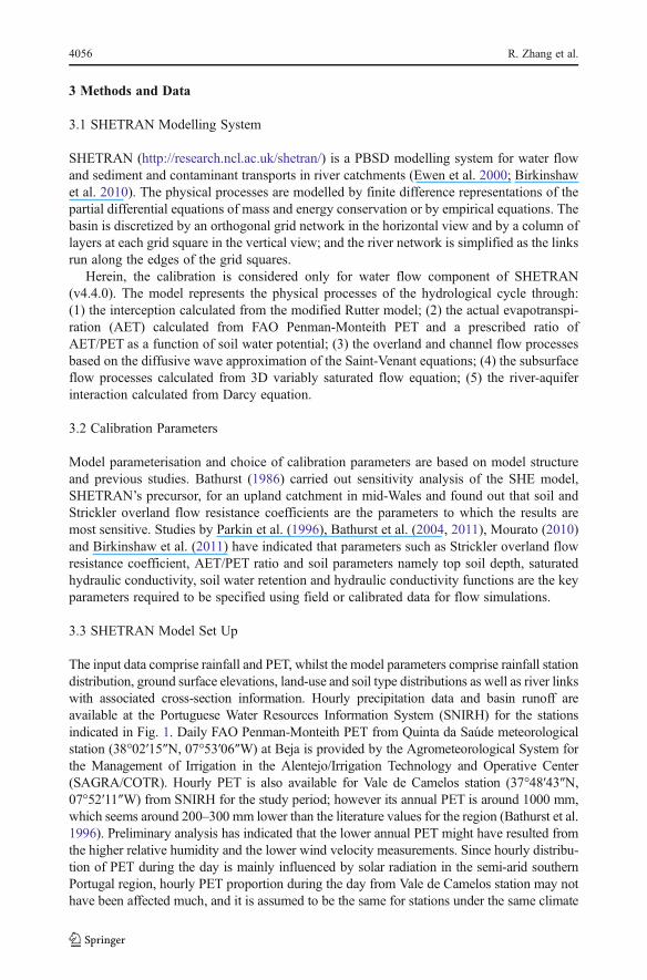
This study is carried out on the part of the Cobres river basin situated above the Monte daPonte gauging station. The basin is, semi-arid, middle-sized with area of 705 km2, located inthe Alentejo province of southern Portugal (37°28′N–37°57′N, 8°10′W–7°51′W, Fig. 1), anarea suffering from desertification (Bathurst et al. 1996). It is a region of relatively low relief,with the elevation varying from 103 to 308 m above sea level. Nine types of soil areidentified, of which the main types are red or yellow Mediterranean soil of Schist origin(Vx soil), brown Mediterranean soil of Schist or Greywacke origin (Px soil) and lithosolsfrom semi-arid and sub-humid climate of Schist or Greywacke origin (Ex soil), occupyingrespectively 20 %, 45 % and 26 % of the basin area. The soils are thin with depth varyingfrom 10 to 50 cm. Four types of land-use are identified, of which the predominant types arecrop (70 %) and agroforestry (27 %). The climate in this region is characteristicallyMediterranean and Continental, with moderate winters and hot and dry summers, high dailytemperature range, and a weak and irregular precipitation regime; mean annual precipitationof rain gauge stations in the region varies between 400 and 900 mm, with around 50 to 80rainy days per year (Ramos and Reis 2001). The mean annual potential evapotranspiration(PET) is around 1300 mm.

Fig. 1 Location map, SHETRAN grid network and channel system (heavy blue lines, representing all channellinks, and light blue lines, representing the links used to extract simulated discharges at basin outlet andinternal gauging stations) for the Cobres basin, showing the rain gauges and gauging stations (the bluetriangles at outlet, northern and central parts of the basin, are respectively Monte da Ponte, Albernoa andEntradas gauging stations). The grid squares have dimensions 2×2 km2

Automatic Calibration of the SHETRAN Hydrological Model 4055

3 Methods and Data

3.1 SHETRAN Modelling System

SHETRAN (http://research.ncl.ac.uk/shetran/) is a PBSD modelling system for water flowand sediment and contaminant transports in river catchments (Ewen et al. 2000; Birkinshawet al. 2010). The physical processes are modelled by finite difference representations of thepartial differential equations of mass and energy conservation or by empirical equations. Thebasin is discretized by an orthogonal grid network in the horizontal view and by a column oflayers at each grid square in the vertical view; and the river network is simplified as the linksrun along the edges of the grid squares.

Herein, the calibration is considered only for water flow component of SHETRAN(v4.4.0). The model represents the physical processes of the hydrological cycle through:(1) the interception calculated from the modified Rutter model; (2) the actual evapotranspi-ration (AET) calculated from FAO Penman-Monteith PET and a prescribed ratio ofAET/PET as a function of soil water potential; (3) the overland and channel flow processesbased on the diffusive wave approximation of the Saint-Venant equations; (4) the subsurfaceflow processes calculated from 3D variably saturated flow equation; (5) the river-aquiferinteraction calculated from Darcy equation.

3.2 Calibration Parameters

Model parameterisation and choice of calibration parameters are based on model structureand previous studies. Bathurst (1986) carried out sensitivity analysis of the SHE model,SHETRAN’s precursor, for an upland catchment in mid-Wales and found out that soil andStrickler overland flow resistance coefficients are the parameters to which the results aremost sensitive. Studies by Parkin et al. (1996), Bathurst et al. (2004, 2011), Mourato (2010)and Birkinshaw et al. (2011) have indicated that parameters such as Strickler overland flowresistance coefficient, AET/PET ratio and soil parameters namely top soil depth, saturatedhydraulic conductivity, soil water retention and hydraulic conductivity functions are the keyparameters required to be specified using field or calibrated data for flow simulations.

3.3 SHETRAN Model Set Up

The input data comprise rainfall and PET, whilst the model parameters comprise rainfall stationdistribution, ground surface elevations, land-use and soil type distributions as well as river linkswith associated cross-section information. Hourly precipitation data and basin runoff areavailable at the Portuguese Water Resources Information System (SNIRH) for the stationsindicated in Fig. 1. Daily FAO Penman-Monteith PET from Quinta da Saúde meteorologicalstation (38°02′15″N, 07°53′06″W) at Beja is provided by the Agrometeorological System forthe Management of Irrigation in the Alentejo/Irrigation Technology and Operative Center(SAGRA/COTR). Hourly PET is also available for Vale de Camelos station (37°48′43″N,07°52′11″W) from SNIRH for the study period; however its annual PET is around 1000 mm,which seems around 200–300 mm lower than the literature values for the region (Bathurst et al.1996). Preliminary analysis has indicated that the lower annual PET might have resulted fromthe higher relative humidity and the lower wind velocity measurements. Since hourly distribu-tion of PET during the day is mainly influenced by solar radiation in the semi-arid southernPortugal region, hourly PET proportion during the day from Vale de Camelos station may nothave been affected much, and it is assumed to be the same for stations under the same climate

4056 R. Zhang et al.

condition. Therefore, the daily PET from Beja is disaggregated into hourly intervals, accordingto the variation of the corresponding hourly PET from Vale de Camelos, to serve as input. Acomprehensive geospatial dataset is available including topographic data with a scale of1:25000 at 10 m intervals, digital maps of land-use type (Caetano et al. 2009) with a scale of1:100000 and soil type (from Institute of Hydraulics, Rural Engineering and Environment,IHERA) with a scale of 1:25000. Here, model calibration and validation are carried outrespectively from October 1st 2004 to September 30th 2006 and from October 1st 2006 toSeptember 30th 2008. The calibration excludes the first 10 months as warm-up period; thevalidation excludes the period from November 4th 2006 to November 8th 2006, due to theexistence of missing data. SHETRAN is applied to the study basin with spatial resolution of2 km grid and temporal resolution of 1 h.

To effectively reduce the number of the calibration parameters, the key parameters areconsidered for calibration of only the two main types of land-use and the three main types of soil,while those for the other types of land-use and soil maintain their baseline values. AET isdetermined by PET, crop characteristics and soil water stress conditions (Allen et al. 1998). TheAET/PET ratio is considered to be maximal at soil field capacity declining linearly with increasingsoil suction. The AET/PET ratio at soil field capacity and Strickler overland flow resistancecoefficient are to be calibrated for the main types of land-use. Anisotropy of soil physical propertiesis not considered, so vertical saturated conductivity is assumed to be the same as the lateralsaturated conductivity. The soil water retention and hydraulic conductivity functions are defined byvan Genuchten et al. (1991). The saturated hydraulic conductivity, saturated water content, residualwater content, van Genuchten n and α parameters, and top soil depth are to be calibrated for themain types of soil. Consequently, twenty-two parameters are to be calibrated by MSCE algorithm.

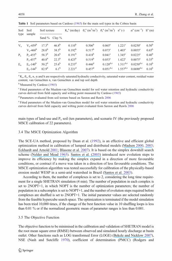
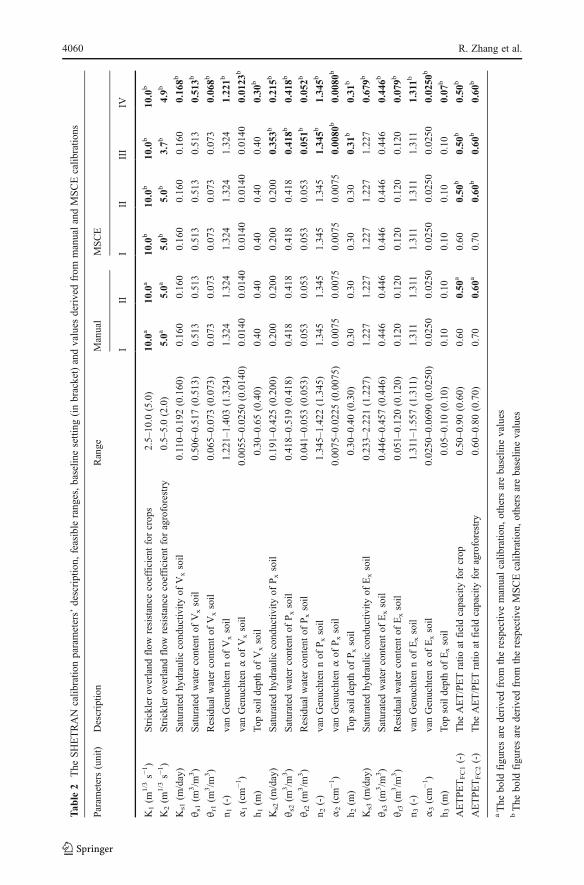
As automatic calibration does not use physical reasoning, the parameter values areconstrained within physically realistic ranges according to field measurements and literaturedata to produce results that can be justified on physical grounds. The measured and estimatedsoil parameters are shown in Table 1. The key parameters for automatic calibration of theCobres basin, with spatial resolution of 2 km grid and temporal resolution of 1 h, are finalized inTable 2, with specified ranges and baseline values based on literature (Cardoso 1965; Bathurstet al. 1996, 2002; Saxton and Rawls 2006), sensitivity analysis and personal communicationwith Dr. Birkinshaw at Newcastle University. According to Allen et al. (1998), the AET/PETratio at field capacity is considered to be in the range of [0.5, 0.9] for crop and [0.6, 0.8] foragroforestry; it is set to 0.6 for crop and 0.7 for agroforestry in baseline simulation. Ramos andSantos (2009) found that the AET/PET ratio is around 0.7 at field capacity for olive orchard insouthern Portugal, which confirmed our AET/PET ratio setting. Based on Engman (1986) andBathurst et al. (1996, 2002), the Strickler overland flow resistance coefficient is set to be in theranges of [2.5, 10] and [0.5, 5.0] m1/3/s respectively for crop and agroforestry; it is set to 5.0 and2.0 m1/3/s respectively for crop and agroforestry in baseline simulation. Based on Chow (1959),the Strickler channel flow resistance coefficient is set to 30 m1/3/s. Sensitivity analysis is carriedout on the 22 parameters in terms ofmodel outputs such as total runoff andNSE. It is shown thatthe results are most sensitive to van Genuchten α, sensitive to AET/PET ratio, Strickleroverland flow resistance coefficient, top soil depth, van Genuchten n, saturated water contentand residual water content, and not so much sensitive to saturated hydraulic conductivity.

To compare the difference of results between manual and automatic calibrations, scenario Iconsiders only calibration of Strickler overland flow resistance coefficient for the two maintypes of land-use (two parameters), scenario II considers calibration of Strickler overland flowresistance coefficient and the AET/PET ratio at field capacity for the twomain types of land-use(four parameters). The differences among MSCE calibration schemes with different parame-terizations are compared: scenarios I and II; scenario III, considering key parameters for two

Automatic Calibration of the SHETRAN Hydrological Model 4057

main types of land-use and Px soil (ten parameters), and scenario IV (the previously proposedMSCE calibration of 22 parameters).

3.4 The MSCE Optimization Algorithm

The SCE-UA method, proposed by Duan et al. (1992), is an effective and efficient globaloptimization method in calibration of lumped and distributed models (Madsen 2000, 2003;Eckhardt and Arnold 2001; Blasone et al. 2007). It is based on the simplex downhill searchscheme (Nelder and Mead 1965). Santos et al. (2003) introduced new evolution steps toimprove its efficiency by making the simplex expand in a direction of more favourableconditions, or contract if a move was taken in a direction of less favourable conditions. TheMSCE optimization algorithm was tested successfully for calibration of the physically-basederosion model WESP in a semi-arid watershed in Brazil (Santos et al. 2003).

According to them, the number of complexes is set to 2, considering the long time require-ment for a single SHETRAN simulation (4 min). The number of population in each complex isset to 2NOPT+1, in which NOPT is the number of optimization parameters; the number ofpopulation in a subcomplex is set to NOPT+1, and the number of evolution steps required beforecomplexes are shuffled is set to 2NOPT+1. The initial parameter values are selected randomlyfrom the feasible hypercube search space. The optimization is terminated if the model simulationhas been tried 10,000 times, if the change of the best function value in 10 shuffling loops is lessthan 0.01 % or if the normalized geometric mean of parameter ranges is less than 0.001.

3.5 The Objective Function

The objective function to be minimised in the calibration and validation of SHETRANmodel isthe root mean square error (RMSE) between observed and simulated hourly discharge at basinoutlet. Other functions such as LOG transformed Error (LOGE) (Bekele and Nicklow 2007),NSE (Nash and Sutcliffe 1970), coefficient of determination (PMCC) (Rodgers and

Table 1 Soil parameters based on Cardoso (1965) for the main soil types in the Cobres basin

Soiltype

Soilsample

Soil texture Ksa (m/day) θs

a (m3/m3) θra (m3/m3) na (-) αa (cm−1) ha (m)

Sand % Clay %

Vx Vx-459b 17.3b 46.8b 0.110b 0.506b 0.065c 1.221c 0.0250c 0.50b

Vx-460b 28.0b 38.5b 0.192b 0.517b 0.073c 1.403c 0.0055c 0.65b

Px Px-455b 58.3b 20.6b 0.191b 0.418b 0.041c 1.345c 0.0225c 0.40b

Px-457b 40.8b 22.3b 0.425b 0.519b 0.053c 1.422c 0.0075c 0.35b

Ex Ex-140b 50.2b 25.6b 0.233d 0.446d 0.120d,e 1.311d,e 0.0250d,e 0.10b

Ex-144b 82.9b 6.1b 2.221d 0.457d 0.051d,e 1.557d,e 0.0690d,e 0.10b

a Ks, θs, θr, n, α and h are respectively saturated hydraulic conductivity, saturated water content, residual watercontent, van Genuchten n, van Genuchten α and top soil depthbMeasured by Cardoso (1965)c Fitted parameters of the Mualem-van Genuchten model for soil water retention and hydraulic conductivitycurves derived from field capacity and wilting point measured by Cardoso (1965)d Parameters evaluated from soil texture based on Saxton and Rawls 2006e Fitted parameters of the Mualem-van Genuchten model for soil water retention and hydraulic conductivitycurves derived from field capacity and wilting point evaluated from Saxton and Rawls 2006

4058 R. Zhang et al.

Nicewander 1988) and index of agreement (IOA) (Willmott 1981) are also calculated toevaluate comprehensively the model performances. In addition, visual fitting of hydrographshas also been performed in manual calibration. RMSE emphasizes fitting of the higher or peakdischarges due to the square to the errors with values greater than 1.0 and LOGE is designed toemphasize fitting of the lower discharges by the introduction of logarithms. Both of them rangebetween 0 (perfect match) and +∞. NSE is a measure of goodness-of-fit and is independent ofthe flow magnitude. It ranges from −∞ to 1 (perfect fit). PMCC measures the variability ofobserved flow that is explained by the model. It ranges from −1 (fully negative correlation) to 1(fully positive correlation). IOA makes cross-comparisons between models or model perfor-mances and it varies between 0 and 1 (perfect fit).

4 Results and Discussion

4.1 MSCE Calibration of SHETRAN Model (Scenario IV)

Scenario IV provides the best set of parameters (Table 2). The parameter values are wellconsistent with literature data. Bathurst et al. (1996) carried out a SHETRAN simulation ofthe Cobres basin for the period from 1977 to 1985; they characterized the basin land-use ascrop (at least 90 % occupation) and the soil type as a thin, poor quality, red Mediterraneansoil overlying schists (corresponding to the Vx soil of this study) with measured saturatedhydraulic conductivity values between 0.03 and 0.4 m/day and depth of A and B horizonsbetween 13 and 33 cm thick. Their calibration indicated that the soil depth is 0.4 m, saturatedhydraulic conductivity is 0.05 m/day and Strickler overland flow resistance coefficient is6 m1/3/s. Here, we carried out hydrological simulation for the period from 2004 to 2008, andcharacterized the basin as two main types of land-use (crop and agroforestry) and three maintypes of soil (Vx, Px and Ex soil). Scenario IV determined that soil depth is 0.30 m, saturatedhydraulic conductivity is 0.168 m/day for Vx soil, which is in agreement with Bathurst et al.(1996). Strickler overland flow resistance coefficient for crop is 10 m1/3/s, which is largerthan that derived by Bathurst et al. (1996) and at the highest limit of its physically realisticrange. Experiment of scenario IV with spatial resolution of 1 km suggests a value of7.0 m1/3/s, which indicated that by using the larger spatial resolution the resulting value ofStrickler overland flow resistance coefficient may become smaller than the highest limit ofits physically realistic range. However, further studies are required to clarify this point.

The result of prescribed AET/PET ratio as a function of soil water potential can also beproperly interpreted by physical reasoning. Scenario IV suggests a value of 0.50 and 0.60respectively for crop and agroforestry at field capacity. The AET/PET ratio was assigned todecline linearly with increasing soil suction. It is 0 at wilting point. Specifically, we assumed−3.3 m as field capacity, −150.0 m as wilting point; then, the AET/PET ratios for crop andagroforestry with soil water potential of −10.0 m are respectively 0.165 and 0.198. Taking the Pxsoil as an example, the calibrated soil water retention curve indicates that soil water content at fieldcapacity, soil water potential of −10.0 m and wilting point are respectively 0.298, 0.228 and0.122 m3/m3. The available water at field capacity and soil water potential of −10.0 m arerespectively 0.176 and 0.106 m3/m3. To access the available water, plants need to exert 3.3 and10.0 m soil suction respectively at field capacity and soil water potential of −10.0 m.Consequently, the AET/PET ratio at soil water potential of −10.0 m is 0.33 times at field capacity.

Model performance of the scenario IV is shown in Table 3; annual mass balance analysisof it is shown in Table 4 for basin outlet and internal gauging stations. For basin outlet, theNSE is 0.86 for calibration and 0.74 for validation; the NSE is respectively 0.65 and 0.82 for

Automatic Calibration of the SHETRAN Hydrological Model 4059

Tab

le2

The

SHETRAN

calib

ratio

nparameters’

description,

feasible

ranges,baselin

esetting

(inbracket)andvalues

derivedfrom

manualandMSCEcalib

ratio

ns

Param

eters(unit)

Descriptio

nRange

Manual

MSCE

III

III

III

IV

K1(m

1/3s−

1)

Strickler

overland

flow

resistance

coefficientforcrop

s2.5–10

.0(5.0)

10.0

a10

.0a

10.0

b10.0

b10.0

b10.0

b

K2(m

1/3s−

1)

Strickler

overland

flow

resistance

coefficientforagroforestry

0.5–5.0(2.0)

5.0a

5.0a

5.0b

5.0b

3.7b

4.9b

Ks1(m

/day)

Saturated

hydraulic

cond

uctiv

ityof

Vxsoil

0.110–0.19

2(0.160

)0.16

00.16

00.16

00.160

0.160

0.168b

θs1(m

3/m

3)

Saturated

water

contentof

Vxsoil

0.50

6–0.51

7(0.513

)0.51

30.51

30.51

30.513

0.513

0.513b

θr1(m

3/m

3)

Residualwater

contentof

Vxsoil

0.06

5–0.07

3(0.073

)0.07

30.07

30.07

30.073

0.073

0.068b

n 1(-)

vanGenuchten

nof

Vxsoil

1.22

1–1.40

3(1.324

)1.32

41.32

41.32

41.324

1.324

1.221b

α1(cm

−1)

vanGenuchten

αof

Vxsoil

0.00

55–0.025

0(0.014

0)0.01

400.01

400.01

400.0140

0.0140

0.0123

b

h 1(m

)Top

soildepthof

Vxsoil

0.30–0.65(0.40)

0.40

0.40

0.40

0.40

0.40

0.30

b

Ks2(m

/day)

Saturated

hydraulic

cond

uctiv

ityof

Pxsoil

0.19

1–0.42

5(0.200

)0.20

00.20

00.20

00.200

0.353b

0.215b

θs2(m

3/m

3)

Saturated

water

contentof

Pxsoil

0.41

8–0.51

9(0.418

)0.41

80.41

80.41

80.418

0.418b

0.418b

θr2(m

3/m

3)

Residualwater

contentof

Pxsoil

0.04

1–0.05

3(0.053

)0.05

30.05

30.05

30.053

0.051b

0.052b

n 2(-)

vanGenuchten

nof

Pxsoil

1.34

5–1.42

2(1.345

)1.34

51.34

51.34

51.345

1.345b

1.345b

α2(cm

−1)

vanGenuchten

αof

Pxsoil

0.00

75–0.022

5(0.007

5)0.00

750.00

750.00

750.0075

0.0080

b0.0080

b

h 2(m

)Top

soildepthof

Pxsoil

0.30–0.40(0.30)

0.30

0.30

0.30

0.30

0.31

b0.31

b

Ks3(m

/day)

Saturated

hydraulic

cond

uctiv

ityof

Exsoil

0.23

3–2.22

1(1.227

)1.22

71.22

71.22

71.227

1.227

0.679b

θs3(m

3/m

3)

Saturated

water

contentof

Exsoil

0.44

6–0.45

7(0.446

)0.44

60.44

60.44

60.446

0.446

0.446b

θr3(m

3/m

3)

Residualwater

contentof

Exsoil

0.05

1–0.12

0(0.120

)0.12

00.12

00.12

00.120

0.120

0.079b

n 3(-)

vanGenuchten

nof

Exsoil

1.311–1.55

7(1.311)

1.311

1.311

1.311

1.311

1.311

1.311b

α3(cm

−1)

vanGenuchten

αof

Exsoil

0.02

50–0.069

0(0.025

0)0.02

500.02

500.02

500.0250

0.0250

0.0250

b

h 3(m

)Top

soildepthof

Exsoil

0.05–0.10(0.10)

0.10

0.10

0.10

0.10

0.10

0.07

b

AETPETFC1(-)

The

AET/PETratio

atfieldcapacity

forcrop

0.50–0.90(0.60)

0.60

0.50

a0.60

0.50

b0.50

b0.50

b

AETPETFC2(-)

The

AET/PETratio

atfieldcapacity

foragroforestry

0.60–0.80(0.70)

0.70

0.60

a0.70

0.60

b0.60

b0.60

b

aThe

bold

figuresarederivedfrom

therespectiv

emanualcalib

ratio

n,others

arebaselin

evalues

bThe

bold

figu

resarederivedfrom

therespectiv

eMSCEcalib

ratio

n,others

arebaselin

evalues

4060 R. Zhang et al.

calibration, 0.69 and 0.63 for validation of internal gauging stations Albernoa and Entradas.The simulation underestimated annual runoff at basin outlet around 11 % (year 2007) to35 % (year 2006). The graphical comparison between observed and simulated discharges atbasin outlet, displayed in Fig. 2a−b for the main runoff periods, during the calibration andvalidation phases, indicates that the model could not catch well the peak discharge for mostof the storm events.

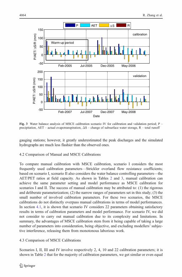
To find out what has happened, we plotted the monthly water balance components for thesimulation in Fig. 3. It is shown that, during the entire period, (1) rainfall mainly concentrated inthe period from October to May of the following year; (2) runoff mainly appeared in 4 months,namely November 2005, October 2006, November 2006 andDecember 2006. It is clear that thetwo main runoff generation periods are respectively preceded by 12 and 6 months’ drought.Therefore, the runoff underestimation may also be explained by the reduced soil infiltrationresulting from the occurrence of surface sealing and crust formation, physical processes that arenot embodied in SHETRAN model, due to the existence of forcing factors such as dry initialsoil moisture content, gentle basin slope, Px and Ex soils (loam and sandy loam) and moderaterainfall intensity. Studies conducted in this region (Silva 2006; Pires et al. 2007) have shownthat Mediterranean soils are characterized by having crust formation problems and lowinfiltration capacity. Soil sealing and crusting are recognized as common processes in cultivatedsoils of semi-arid and arid regions. Since the study basin is mainly occupied by crops, thecrusting formation problems might have been very important in this region. However, the crustformation problem is not considered in this study due to the lack of information for quantifyinghow much infiltration would be reduced by soil crust considering the nature of the rain, thesoil’s physical and chemical properties of the Cobres basin during the study period.Experiments show that the overall model performance would not be improved by arbitrarilyreducing saturated hydraulic conductivity for the whole simulation period.

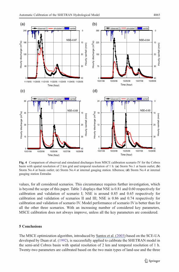
Figure 4a−d are made to get a clear impression of SHETRAN’s ability to reproduce thestorm events preceded by long period of drought. Storms No.1 and No.4 are the largest stormevents respectively during the calibration and validation periods. Figure 4a−b are respectivecomparisons of observed and simulated hydrographs for storms No.1 and No.4 at basin outlet;

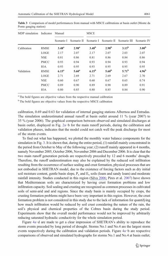
Table 3 Comparison of model performances from manual with MSCE calibrations at basin outlet (Monte daPonte gauging station)

MDP simulation Indicator Manual MSCE

Scenario I Scenario II Scenario I Scenario II Scenario III Scenario IV

Calibration RMSE 3.48a 2.98a 3.48b 2.98b 3.13b 3.00b

LOGE 2.17 2.07 2.17 2.07 2.03 2.07

NSE 0.81 0.86 0.81 0.86 0.84 0.86

PMCC 0.93 0.94 0.93 0.94 0.93 0.94

IOA 0.93 0.95 0.93 0.95 0.95 0.95

Validation RMSE 6.15a 5.60a 6.15b 5.60b 5.71b 4.96b

LOGE 2.71 2.69 2.71 2.69 2.67 2.70

NSE 0.60 0.67 0.60 0.67 0.65 0.74

PMCC 0.89 0.90 0.89 0.90 0.89 0.91

IOA 0.80 0.85 0.80 0.85 0.84 0.90

a The bold figures are objective values from the respective manual calibrationb The bold figures are objective values from the respective MSCE calibration

Automatic Calibration of the SHETRAN Hydrological Model 4061

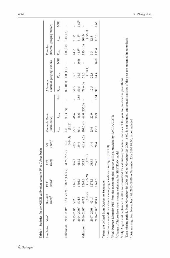
Tab

le4

StatisticsfortheMSCEcalib

ratio

nscenario

IVat

Cob

resbasin

Sim

ulation

Yeara

Rainfall

(mm)b

PET

(mm)c

AET

(mm)

ΔS

(mm)d

Mon

teda

Ponte

(Basin

outlet)

Alberno

a(Internalgaug

ingstation)

Entradas

(Internalgaugingstation)

Robs

Rsim

NSE

Robs

Rsim

NSE

Robs

Rsim

NSE

Calibratio

n2004–200

5e1.8(194.2)

358.2(1475.7)

31.9

(256

.7)

−30.1

(−64

.5)

0.0 (11.6)

0.0(1.9)

–0.0(0.1)

0.0(1.1)

–0.0(0.0)

0.0(1.4)

–

2005–200

650

2.5

1345

.838

6.3

69.5

55.1

46.6

–50

.536

.3–

44.8g

31.8g

–

2004–200

6e50

4.3

1704

.041

8.2

39.4

55.1

46.6

0.86

50.5

36.3

0.65

44.8g

31.8g

0.82

g

Validation

2006–200

7f44

7.2

(532.2)

1267

.6(1272.9)

373.2

(378

.3)

6.0(18.2)

104.5(-)

68.0

(135

.5)

–79

.6(-)

71.6 (138

.4)

–13

0.1(-)

104.0

(195.1)

–

2007–200

842

1.4

1274

.138

3.4

14.4

25.6

22.9

–12

.522

.8–

5.3

12.3

–

2006–200

8f86

8.7

2541

.775

6.6

20.4

130.1

90.9

0.74

92.1

94.4

0.69

135.4

116.3

0.63

aYears

aredefinedfrom

October

toSeptember

bBasin

meanrainfallbasedon

sixrain

gauges

indicatedin

Fig.1(SNIRH)

cFA

OPenman-M

onteith

PETfrom

themeteorologicalstationat

Beja,provided

bySAGRA/COTR

dChang

eof

Sub

surfacewater

storagecalculated

bySHETRAN

mod

eleOnlyAugustandSeptemberin

2005

areconsidered

forcalib

ratio

n,andannual

statisticsof

theyear

arepresentedin

parenthesis

fDatamissing

period,from

Novem

ber4th2006

23:00to

Novem

ber8th2006

16:00,

isnotincluded,andannual

statisticsof

theyear

arepresentedin

parenthesis

gDatamissing

,from

Nov

ember19

th20

0509

:00to

Nov

ember25

th20

0509

:00,

isno

tincluded

4062 R. Zhang et al.

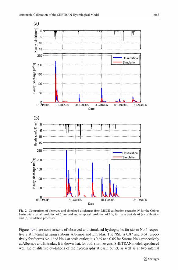
Figure 4c−d are comparisons of observed and simulated hydrographs for storm No.4 respec-tively at internal gauging stations Albernoa and Entradas. The NSE is 0.87 and 0.64 respec-tively for Storms No.1 and No.4 at basin outlet; it is 0.69 and 0.65 for Storms No.4 respectivelyat Albernoa and Entradas. It is shown that, for both storm events, SHETRANmodel reproducedwell the qualitative evolutions of the hydrographs at basin outlet, as well as at two internal

Fig. 2 Comparison of observed and simulated discharges from MSCE calibration scenario IV for the Cobresbasin with spatial resolution of 2 km grid and temporal resolution of 1 h, for main periods of (a) calibrationand (b) validation processes

Automatic Calibration of the SHETRAN Hydrological Model 4063

gauging stations; however, it greatly underestimated the peak discharges and the simulatedhydrographs are much less flashier than the observed ones.

4.2 Comparison of Manual and MSCE Calibrations

To compare manual calibration with MSCE calibration, scenario I considers the mostfrequently used calibration parameters—Strickler overland flow resistance coefficients;based on scenario I, scenario II also considers the water balance controlling parameters—theAET/PET ratios at field capacity. As shown in Tables 2 and 3, manual calibration canachieve the same parameter setting and model performance as MSCE calibration forscenarios I and II. The success of manual calibration may be attributed to: (1) the rigorousand deliberate parameterization; (2) the narrow ranges of parameters set in this study; (3) thesmall number of involved calibration parameters. For these two scenarios, the MSCEcalibrations do not distinctly overpass manual calibrations in terms of model performances.In section 4.1, it is shown that scenario IV considers 22 parameters obtaining satisfactoryresults in terms of calibration parameters and model performance. For scenario IV, we didnot consider to carry out manual calibration due to its complexity and limitations. Insummary, the advantages of MSCE calibration stem from it being capable of taking a largenumber of parameters into consideration, being objective, and excluding modellers’ subjec-tive interference, releasing them from monotonous laborious work.

4.3 Comparison of MSCE Calibrations

Scenarios I, II, III and IV involve respectively 2, 4, 10 and 22 calibration parameters; it isshown in Table 2 that for the majority of calibration parameters, we get similar or even equal

Feb-2005 Jul-2005 Dec-2005 May-2006-50

0

50

100

150

P/A

ET

/ΔS

/R (

mm

)

Feb-2007 Jul-2007 Dec-2007 May-2008-50

0

50

100

150

200

Date

P/A

ET

/ΔS

/R (

mm

)

P AET S R

Warm-up period

validation

calibration

Δ

Fig. 3 Water balance analysis of MSCE calibration scenario IV for calibration and validation period; P –precipitation, AET – actual evapotranspiration, ΔS – change of subsurface water storage, R – total runoff

4064 R. Zhang et al.

values, for all considered scenarios. This circumstance requires further investigation, whichis beyond the scope of this paper. Table 3 displays that NSE is 0.81 and 0.60 respectively forcalibration and validation of scenario I; NSE is around 0.85 and 0.65 respectively forcalibration and validation of scenarios II and III; NSE is 0.86 and 0.74 respectively forcalibration and validation of scenario IV. Model performance of scenario IV is better than forall the other three scenarios. With an increasing number of considered key parameters,MSCE calibration does not always improve, unless all the key parameters are considered.

5 Conclusions

The MSCE optimization algorithm, introduced by Santos et al. (2003) based on the SCE-UAdeveloped by Duan et al. (1992), is successfully applied to calibrate the SHETRAN model inthe semi-arid Cobres basin with spatial resolution of 2 km and temporal resolution of 1 h.Twenty-two parameters are calibrated based on the two main types of land-use and the three

(a)

11/19/05 11/20/05 11/21/05 11/22/05 11/23/05 11/24/05 11/25/05

0

60

120

180

240

Time (hour)

Hourly d

ischarg

e (

m3/s

) NSE=0.87

0

10

20

30

40

Hourly r

ain

fall

(mm

)

observed Q simulated Q rainfall

(b)

10/21/06 10/23/06 10/25/06 10/27/06 10/29/060

75

150

225

300

Time (hour)

Hourly d

ischarg

e (

m3/s

) NSE=0.64

0

10

20

30

40

Hourly r

ain

fall

(mm

)

observed Q simulated Q rainfall

(c)

10/21/06 10/23/06 10/25/06 10/27/06 10/29/060

15

30

45

60

Time (hour)

Ho

urly d

isch

arg

e (

m3/s

) NSE=0.69

0

10

20

30

40

Ho

urly r

ain

fall

(mm

)

observed Q simulated Q rainfall

(d)

10/21/06 10/23/06 10/25/06 10/27/06 10/29/060

6

12

18

24

Time (hour)

Hourly d

ischarg

e (

m3/s

) NSE=0.65

0

10

20

30

40

Hourly r

ain

fall

(mm

)

observed Q simulated Q rainfall

Fig. 4 Comparison of observed and simulated discharges from MSCE calibration scenario IV for the Cobresbasin with spatial resolution of 2 km grid and temporal resolution of 1 h: (a) Storm No.1 at basin outlet; (b)Storm No.4 at basin outlet; (c) Storm No.4 at internal gauging station Albernoa; (d) Storm No.4 at internalgauging station Entradas

Automatic Calibration of the SHETRAN Hydrological Model 4065

main types of soil, and no initial parameter setting is provided. The calibrated parameters arewithin measured ranges of Cardoso (1965), well consistent with previous work of Bathurstet al. (1996) and well explained by physical reasoning. The results are very satisfactory. NSEis 0.86 for calibration and 0.74 for validation for basin outlet; NSE is respectively 0.65 and0.82 for calibration, 0.69 and 0.63 for validation of internal gauging stations Albernoa andEntradas; as for storm events, NSE is 0.87 and 0.64 respectively for Storms No.1 (during thecalibration period) and No.4 (during the validation period) at basin outlet; it is 0.69 and 0.65for Storm No.4 respectively at Albernoa and Entradas. As a confirmation to the study ofSantos et al. (2003), the MSCE optimization algorithm is able to converge to the globaloptimal values.

For SHETRAN model, manual calibration can be successful if the rigorous and deliberateparameterization has been carried out and a few parameters are involved. MSCE is recom-mended due to the following advantages: being capable of taking a large number ofparameters into consideration, being objective, excluding modellers’ subjective interferenceand releasing them to other more important activities. To get the best model performance, allkey parameters should be considered in MSCE calibration. Future studies should includeother automatic calibration techniques, such as simulated annealing (Santos et al. 2012) andconsider the influence of catchment discretization (Santos et al. 2011) especially whenapplying GIS and remote sensing techniques (Silva et al. 2012).

Acknowledgments This study was made possible by a PhD grant of Portuguese Foundation for Science andTechnology (SFRH/BD/48820/2008). The authors are grateful for the support from the ERLAND (PTDC/AAC-AMB/100520/2008) and CISA (MCT/CT-Hidro, Brazil) projects. The authors thank SNIRH andSAGRA/COTR for providing the necessary data, and the following for the great assistance and helpfuldiscussion during the preparation of this paper: Prof. Kilsby, Dr. Bathurst, Dr. Birkinshaw, Dr. O’Donnell andDr. Bovolo at Newcastle University, UK; Prof. Santos, Prof. Sampaio, Prof. Serralheiro, Prof. Shahidian, Dr.Lima, Dr. Toureiro at University of Évora and Dr. Nunes at University of Aveiro, Portugal. Finally, twoanonymous reviewers are thanked for their comments, which allowed a significant improvement of the paper.

References

Allen RG, Pereira LS, Raes D, Smith M (1998) Crop evapotranspiration: Guidelines for computing crop waterrequirements, FAO irrigation and drainage paper 56. Rome, Italy

Bathurst JC (1986) Sensitivity analysis of the Systeme Hydrologique Europeen for an upland catchment. JHydrol 87:103–123

Bathurst JC, Kilsby C, White S (1996) Modelling the impacts of climate and land-use change on basinhydrology and soil erosion in Mediterranean Europe. In: Brandt CJ, Thornes JB (eds) Mediterraneandesertification and land use. John Wiley & Sons Ltd, Chichester, pp 355–387

Bathurst JC, Sheffield J, Vicente C, White SM, Romano N (2002) Modelling large basin hydrology andsediment yield with sparse data: the Agri basin, southern Italy. In: Geeson NA, Brandt CJ, Thornes JB(eds) Mediterranean desertification: a mosaic of processes and responses. John Wiley & Sons Ltd,Chichester, pp 397–415

Bathurst JC, Ewen J, Parkin G, O’Connell PE, Cooper JD (2004) Validation of catchment models forpredicting land-use and climate change impacts. 3. Blind validation for internal and outlet responses. JHydrol 287:74–94

Bathurst JC, Birkinshaw SJ, Cisneros F, Fallas J, Iroumé A, Iturraspe R, Novillo MG, Urciuolo A, AlvaradoA, Coello C, Huber A, Miranda M, Ramirez M, Sarandón R (2011) Forest impact on floods due toextreme rainfall and snowmelt in four Latin American environments 2: model analysis. J Hydrol400:292–304

Bekele EG, Knapp HV (2010) Watershed modeling to assessing impacts of potential climate change on watersupply availability. Water Resour Manag 24:3299–3320

4066 R. Zhang et al.

Bekele EG, Nicklow JW (2007) Multi-objective automatic calibration of SWAT using NSGA-II. J Hydrol341:165–176

Beven K, Warren R, Zaoui J (1980) SHE: towards a methodology for physically-based distributed forecastingin hydrology. IAHS-AISH Publ 129:133–137

Birkinshaw SJ, James P, Ewen J (2010) Graphical user interface for rapid set-up of SHETRAN physically-based river catchment model. Environ Model Softw 25:609–610

Birkinshaw SJ, Bathurst JC, Iroumé A, Palacios H (2011) The effect of forest cover on peak flow andsediment discharge ─ an integrated field and modelling study in central-southern Chile. Hydrol Process25(8):1284–1297

Blasone RS, Madsen H, Rosbjerg D (2007) Parameter estimation in distributed hydrological modelling:comparison of global and local optimisation techniques. Nord Hydrol 38(4–5):451–476

Bovolo CI, Abele SJ, Bathurst JC, Caballero D, Ciglan M, Eftichidis G, Simo B (2009) A distributedframework for multi-risk assessment of natural hazards used to model the effects of forest fire onhydrology and sediment yield. Comput Geosci 35:924–945

Caetano M, Nunes V, Nunes A (2009) CORINE land cover 2006 for continental Portugal. Instituto GeográficoPortuguês. Technical Report

Cardoso C (1965) Solos de Portugal: sua classificação, caracterização e génese 1 – a sul do rio tejo. Lisbon, PortugalChow VT (1959) Open-channel hydraulics. International Student Edition, McGraw-HillDuan Q, Sorooshian S, Gupta V (1992) Effective and efficient global optimization for conceptual rainfall-

runoff models. Water Resour Res 28(4):1015–1031Eckhardt K, Arnold JG (2001) Automatic calibration of a distributed catchment model. J Hydrol 251:103–109Engman ET (1986) Roughness coefficients for routing surface runoff. Proc Am Soc Civ Eng, J Irrig Drain Eng

112:39–53Ewen J, Parkin G (1996) Validation of catchment models for predicting land-use and climate change impacts.

1. Method. J Hydrol 175:583–594Ewen J, Parkin G, O’Connell PE (2000) SHETRAN: distributed river basin flow and transport modeling

system. J Hydrol Eng 5:250–258Madsen H (2000) Automatic calibration of a conceptual rainfall-runoff model using multiple objectives. J

Hydrol 235:276–288Madsen H (2003) Parameter estimation in distributed hydrological catchment modelling using automatic

calibration with multiple objectives. Adv Water Resour 26:205–216Mourato S (2010) Modelação do impacte das alterações climáticas e do uso do solo nas bacias hidrográficas

do Alentejo. PhD dissertation. University of Évora, PortugalNash JE, Sutcliffe JV (1970) River flow forecasting through conceptual models part I - a discussion of

principles. J Hydrol 10:282–290Nelder JA, Mead R (1965) A simplex method for function minimization. Comput J 7:308–313Parkin G, O’Donnell G, Ewen J, Bathurst JC, O’Connell PE, Lavabre J (1996) Validation of catchment

models for predicting land-use and climate change impacts. 2. Case study for a Mediterranean catchment.J Hydrol 175:595–613

Pires RO, Reis JL, Santos FL, Castanheira NL (2007) Polyacrylamide application in center pivot irrigationsystems for erosion and runoff control. Rev Ciências Agrárias 30(1):172–178

Ramos C, Reis E (2001) As cheias no sul de Portugal em diferentes tipos de bacias hidrográficas. FinisterraXXXVI 71:61–82

Ramos AF, Santos FL (2009) Water use, transpiration, and crop coefficients for olives (cv. Cordovil), grown inorchards in southern Portugal. Biosyst Eng 102:321–333

Refsgaard JC (1997) Parameterisation, calibration and validation of distributed hydrological models. J Hydrol198:69–97

Rodgers JL, Nicewander WA (1988) Thirteen ways to look at the correlation coefficient. Am Stat 42:59–66Santos CAG, Srinivasan VS, Suzuki K, Watanabe M (2003) Application of an optimization technique to a

physically based erosion model. Hydrol Process 17(5):989–1003Santos CAG, Freire PKMM, Silva RM, Arruda PM, Mishra SK (2011) Influence of the catchment

discretization on the optimization of runoff-erosion modelling. J Urban Environ Eng 5(2):91–102Santos CAG, Freire PKMM, Arruda PM (2012) Application of a simulated annealing optimization to a

physically based erosion model. Water Sci Technol 66(10):2099–2108Saxton KE, Rawls WJ (2006) Soil water characteristic estimates by texture and organic matter for hydrologic

solutions. Soil Sci Soc Am J 70:1569–1578Shi P,MaX, HouY, LiQ, Zhang Z, Qu S, ChenC, Cai T, FangX (2013) Effects of land-use and climate change on

hydrological processes in the upstream of Huai river, China. Water Resour Manag 27:1263–1278Silva LL (2006) The effect of spray head sprinklers with different deflector plates on irrigation uniformity,

runoff and sediment yield in a Mediterranean soil. Agric Water Manag 85(3):243–252

Automatic Calibration of the SHETRAN Hydrological Model 4067

Silva RM, Montenegro SMGL, Santos CAG (2012) Integration of GIS and remote sensing for estimation ofsoil loss and prioritization of critical sub-catchments: a case study of Tapacurá catchment. Nat Hazard62(3):953–970

van Genuchten MT, Leij FJ, Yates SR (1991) The RETC code for quantifying the hydraulic functions ofunsaturated soils, report no: EPA/600/2-91/065. Robert S. Kerr Environmental Research Laboratory, U.S.Environmental Protection Agency, Ada

Willmott CJ (1981) On the validation of models. Phys Geogr 2:184–194

4068 R. Zhang et al.

All in-text references underlined in blue are linked to publications on ResearchGate, letting you access and read them immediately.