reconciling port and flag state control over cruise ship onboard ...

Under consideration for publication in J. Fluid Mech. 1
Absolute/Convective instability of a flappingflag
By SANKHA BANERJEE, AND DICK K. P. YUE†Department of Mechanical Engineering, Massachusetts Institute of Technology, Cambridge,
MA 02139, USA
(Received 3 July 2013)
The work presents the study of the nature of instability, whether absolute or convec-tive of a two-dimensional flapping filament submerged in a uniform inflow. When thestructure-to-fluid mass ratio, µ = ρsh/(ρfL) is zero, two waves equal in magnitude andopposite signs exist. We show by constructing an energy conservation law for the lin-earized equations of motion that both types of waves have initially positive energy in thesense that they both require an energy source to be sustained, after a critical value of µ isexceeded the slow waves acquire negative energy, requiring an energy sink for sustainance.With increasing µ for fixed Re = V L/ν = 1000, a flapping instability is sustained bythe coalescence between the fast (positive energy) and the slow (negative energy) wavescreating waves with zero energy which do not require neither an energy source nor a sinkto be sustained, and grow exponentially in time. For almost all values of the µ and Re,the instability was found absolute except a narrow range of µ 0.060 6 µ 6 0.075 overwhich convective instability prevailed. This unstable flapping amplitude at the instabilitythreshold is found to satisfy the linearly unstable Klein-Gordon equation.
1. Introduction
As emphasized in a recent review Shelley & Zhang (2011), the flapping of flag is consid-ered as a canonical problem for studying the instability propagation in numerous physicalsystems where the dynamics of a slender structure is coupled to an axial flow. Landahl(1962) and Benjamin (1963), started such analysis giving rise to a profusion of instabilitytypes in simple physical models. This theoretical framework, was introduced in hydrody-namics by Huerre & Monkewitz (1990), and has been fruitfully applied to fluid-structureinteractions problems. The generic case of inviscid elastic plate, further referred to as theflat-plate problem, has been extensively analyzed (Brazier-Smith & Scott (1984);Carpen-ter & Garrad (1986);Crighton et al. (1991); Lucey & Carpenter (1992); Peake (2003))and extended to membranes under tension by ?). These analyses have brought to lightmany of the fundamental features of these interactions, such as the existence of negativeenergy waves or possible violations of the usual out-going wave radiation condition.
Two different approaches are commonly used to study the instability properties of suchsystems. The first approach considers the medium to be of infinite length, in this case thewaves propagating in the medium are considered through the analysis of the local waveequation. If temporally amplified waves are identified the medium is said to be locallyunstable. Depending on the long time impulse response of the locally unstable medium,two types of instabilities may be distinguished: convective or absolute. The second ap-proach considers the same medium, but of finite length. The modes are studied, through
† Author to whom correspondence should be addressed: [email protected]

2 S. Banerjee and Dick K. P. Yue
the analysis of the same local wave equation, associated with boundary conditions. If atemporally amplified mode is found, the system is said to be globally unstable.
Comparatively little attention has been paid to the question of wave propagation in flagflapping instabilities. Several recent experiments (Zhang et al. (2000); Watanabe et al.(2002); Shelley & Zhang (2011); Eloy et al. (2007)), simulations and models (Theodorsen& Garrick (1940); Zhu & Peskin (2002); Argentina & Mahadevan (2005); Alben & Shelley(2008) and Connell & Yue (2007)) have studied how a flag flaps in a flow. The case ofmultiple flags allows for the interesting possibility of different forms of synchronizationbetween the flags as a function of the distance between the flags. At different transversedistances, phase differences of approximately zero and π between the flapping flags wereobserved in experiment by Zhang et al. (2000) and in simulations by Zhu & Peskin (2002).The phenomena of inverse hydrodynamic drafting, for which flexible bodies enjoy dragincrease when situated behind a leader in a flow can be better explained when the natureof convective/absolute instabilities is better understood in flapping flag systems.
A physical interpretation of a flapping instability implies a small hump, which occurssomewhere along the flag, accelerates the flow resulting in a pressure-drop. This createsa lift force that tends to further increase the size of the hump, if the lift force becomessufficiently strong enough to overcome the structural restoring forces, instability occurs.This interpretation is the simplest way to explain the instability, however it is desirableto obtain an interpretation in terms of the properties of the flapping waves, which consistof an elastic wave on the flag coupled with a pressure wave in the fluid. In this work,the instability mechanism is investigated under the assumption that the flag is infinitelylong. In practical applications the structure has of course always-finite extent, and it iswell known that boundary conditions can often become very important for the flappinginstability. In several practical applications, however, the structure is so long, that theflag to a first approximation can be modeled as an infinitely long structure. For such anapproximation any localized excitation will require a very long time before it reaches theends, and the flag could be thought of as infinite. An important, reason for studying the2D flag problem is because of its simplicity, it is very useful in exploring basic instabilityconcepts that are of more general interest. In fact, Eq. (2.1) is, to the authors knowledge,the simplest equation exhibiting in a nontrivial manner the important features of reactiveinstabilities, whereas at the same time its terms have a direct physical interpretation.Moreover the flapping instability considered here has important common features withother more complicated physical problems, and it is shown that the obtained physicalcriterion is of a certain class of instability problems resulting from the interaction ofpositive and negative energy waves. The goal of the present work is to systematicallydetermine for the first time whether convective or absolute nature of instabilities mayarise in a 2D flapping flag immersed in a uniform flow, as a function of several physicalparameters such as the mass ratio, the flow-induced tension, and the flow velocity. Thevariety of possible transitions is illustrated by considering the general case as well as theextreme values of the non-dimensional parameters. The theoretical analysis provides aguideline for systematic numerical study to identify the characteristic wake structure andfluid flow features in the different regimes of instability.
The work is organized as follows. Section 2 defines the problem we consider andthe relevant system parameters. The linear stability analysis is given in § 3. The ab-solute/convective character of the flapping instability is investigated analytically, andthe character of the instability is determined as a function of the basic nondimensionalparameters involved. A systematic set of FSDS2D results validating the linear stabilitypredictions, and elucidating the coupled structural and vortex behavior of the system arepresented in § 4. Concluding remarks are in § 5.

Absolute/Convective instability of a flapping flag 3
Figure 1. Depiction of the problem of the flapping two-dimensional flag of length L in uniformincoming flow V in an unbounded fluid domain. The flag is pinned at the leading edge and freeat the trailing edge.
2. Problem Statement
We consider the problem of a two-dimensional thin membrane as studied by Connell &Yue (2007), pinned on the leading edge and free on the trailing edge, excited by a uniformincompressible viscous inflow in an unbounded domain, shown in figure 1. The body issufficiently thin so that the small thickness (and its variation with length) is unimportantto the result. The structural properties of the membrane in this two-dimensional study arethe length, mass-per-length, bending rigidity, and extensional rigidity. The extensionalrigidity is considered to be very high, and is included in the nonlinear numerical modelas a means of maintaining continuity and transmitting force tangentially, as detailedin §Connell (2006).
The geometrically nonlinear equation of motion for the two-dimensional flag is
ρsh∂2x
∂t2− ∂
∂s
(T (s)
∂x
∂s
)+ EI
∂4x
∂s4= Ff , (2.1)
with s as the Lagrangian coordinate along the length, and the body position vector xfixed at the pinned leading edge. Here, ρs is the structural density, h is the flag thickness,T (s) is the tension in the body, and EI is the structural bending rigidity. Fluid couplingcomes through the forcing term defined as
Ff = [∆τ ]n, (2.2)
where n is the upward facing normal and [∆τ ] is the difference between the fluid-dynamicstress tensor at the top and bottom of the body. Elements of the stress tensor are definedby the fluid dynamics at the body surface as
τij = νρf
(∂ui∂ξj
+∂uj∂ξi
)− δijp. (2.3)
Equations (2.2) and (2.3) contain all of the physical influence of the fluid flow on theflexible structure. This includes viscous damping and boundary-layer drag, inertial addedmass effect, and the influence of separation and vortices shedding into the wake.
The fluid dynamics are obtained as the solution to the incompressible fluid momentumand mass conservation equations, the Navier-Stokes equations, written as

4 S. Banerjee and Dick K. P. Yue
∂v
∂t+ (v · ∇)v = − 1
ρf∇p+ ν∇2v, (2.4)
∇ · v = 0. (2.5)
The velocity boundary conditions complete the problem specification:
v =∂x
∂ton flag boundary (2.6)
v = V at ∞. (2.7)
It is through this inner boundary condition (2.6) that the structural influence is im-parted to the fluid, so that the flow solution is consistent with the structural motion.While dynamic continuity between the fluid and structural domains is contained in (2.1)-(2.3), kinematic continuity between the domains is contained in (2.4)-(2.7). This set ofequations governs the coupled fluid and structural motion of the system depicted infigure 1.
3. Theoretical Results: Local Stability (LSA)
3.1. The Onset of Instability
Following the work of Connell & Yue (2007), Triantafyllou (1992) and Coene (1992), wecan write the equation of motion for a 2D flag, considering z to be the displacement fromthe streamwise y axis, as:
ρsh∂2z
∂t2− ∂
∂y
(T∂z
∂y
)+ EI
∂4z
∂y4+ma
(∂
∂t+ V
∂
∂y
)2
z = 0. (3.1)
We have allowed for variation of the tension in the streamwise direction. Unlike thesoap film problem where gravity influences the tension, the present study has only thefluid forcing contributing to the tension. Assuming the fluid forcing to be that due to aBlasius laminar boundary layer, the tension can be written as:
T (y) = 1.3ρfV2LRe−1/2
(1−
√y
L
), (3.2)
where
Re =V L
ν. (3.3)
In seeking a solution to (3.1) we avoid the variable tension expression of (3.2), insteaduse the maximum value of (3.2) evaluated at y = 0 as a constant value along the length.
The equation of motion is now written with the last term can be expanded as:
ρsh∂2z
∂t2− 1.3ρfV
2LRe−1/2∂2z
∂y2+ EI
∂4z
∂y4
+ ma∂2z
∂t2+ 2maV
∂2z
∂y∂t+maV
2 ∂2z
∂y2= 0. (3.4)
The three expanded final terms represent the fluid-dynamic effects of inertial addedmass, Coriolis force, and centrifugal force, respectively (see Triantafyllou 1992).

Absolute/Convective instability of a flapping flag 5
Grouping the terms we have:
(ρsh+ma)∂2z
∂t2+ (maV
2 − 1.3ρfV2LRe−1/2)
∂2z
∂y2+ EI
∂4z
∂y4+ 2maV
∂2z
∂y∂t= 0. (3.5)
In the second term, the countering effects of the Kelvin-Helmholtz instability andthe restoring action of the drag-induced tension can be seen. The variables (y, z, t) of theequation of motion are now non dimensionalized by the length L and free stream velocityV , obtaining:
(ρsh+ma)V 2
L
∂2z
∂t2+ (maV
2 − 1.3ρfV2LRe−1/2)
1
L
∂2z
∂y2+ EI
1
L3
∂4z
∂y4
+2maVV
L
∂2z
∂y∂t= 0. (3.6)
Dividing through by V 2ρf we obtain the final form of the nondimensional equation:
(µ+ cm)∂2z
∂t2+(cm − 1.3Re−1/2
) ∂2z∂y2
+KB∂4z
∂y4+ 2cm
∂2z
∂y∂t= 0, (3.7)
where cm = ma/(ρfL).We assume a travelling-wave mode, z = Aei(ky−ωt), where k and ω are the nondi-
mensional wavenumber and frequency. The equation of motion then yields the dispersionrelation:
D(ω, k) = (µ+ cm)ω2 +(cm − 1.3Re−1/2
)k2 −KBk
4 − 2cmωk = 0. (3.8)
Solving for the frequency, we have:
ω1,2 =cmk
µ+ cm± 1
µ+ cm
√c2mk
2 − (µ+ cm)(cmk2 − 1.3Re−1/2k2 −KBk4
)(3.9)
=cmk
µ+ cm± k
µ+ cm
√−µcm + (µ+ cm)
(1.3Re−1/2 +KBk2
).
where the subscripts 1, 2 in the left-hand side of Eq. 3.10 correspond to the plusand minus signs, respectively, in the right-hand side. If for any fixed non-dimensionalparameters there exists some range of real k that yield complex ω, the system is unstable.For (3.10) this occurs when the quantity under the square root can become negative; thisbecomes possible, and unstable flapping modes are realized when the argument of theradical in (??) is negative, i.e.:
µcmµ+ cm
> 1.3Re−1/2 +KBk2. (3.10)
As expected, we see from (??) that the tension and bending rigidity are stabilizingeffects, while the centrifugal force is the destabilizing effect of the Kelvin-Helmholtzinstability. An additional stabilizing effect comes from the Coriolis force (the first termin the radical), which scales only with the added mass. As the expression in the radicalcan never become negative when µ = 0, the system cannot realize unstable flappingwithout structural mass as pointed out by Connell & Yue (2007). The fluid added massis advected with the flow velocity, and, thus, influences the system differently from thestructural mass. It is, in fact, the added mass, which brings about the flapping instability,

6 S. Banerjee and Dick K. P. Yue
but this instability cannot be realized on a massless body. The instability starts as a staticdivergence when (µcm)/(µ+ cm) = 1.3Re−1/2 +KBk
2.As the value of µ is increased above this value, a range of unstable wave numbers
develops, given by
|k| < kc = {[µcm − (µ+ cm)1.3Re−1/2]/(µ+ cm)KB}1/2 (3.11)
For k lying in this range, complex frequencies are obtained with nonzero real parts andpositive imaginary parts. The flapping instability becomes therefore oscillatory.
From potential flow solution, the added mass coefficient for an infinite waving plate isgiven by (Coene 1992):
cm =ma
ρfL=
2
k. (3.12)
The added mass is thus a function of the nondimensional wavenumber and dependenton the flapping mode. The criterion for existence of flapping in the flag can now berewritten in terms of the mode as:
µ12µk + 1
> 1.3Re−1/2 +KBk2. (3.13)
Equation (3.13) shows the stabilizing effect of decreasing mass ratio (the left-hand-sideterm decreases with decreasing µ), decreasing Reynolds number, and increasing bendingrigidity. Zhang et al. (2000) and Zhu & Peskin (2002) found that increasing the lengthis destabilizing, an adjustment which increases Re and decreases KB . These changes toRe and KB are both destabilizing, and the observed trend comes from the combinationof the effects.
Rearranging (3.13), Connell & Yue (2007) obtained the critical mass ratio:
µ =1.3Re−1/2 +KBk
2
1− 0.65Re−1/2k − 0.5KBk3, (3.14)
above which flapping will be realized. In the limiting cases (i) where the mass ratiois small compared to the added mass, they found from (3.10) the critical mass ratio toreduce to:
µ = 1.3Re−1/2 +KBk2. (3.15)
(ii) When the bending rigidity can be neglected, the existence of flapping becomes afunction of only the two parameters µ and Re, and flapping occurs above the criticalmass ratio given by:
µ = 1.3Re−1/2. (3.16)
A plot of the stability relation (3.14) is shown in figure 2, depicting the relationshipbetween the critical mass ratio µ and bending rigidity KB for the k = 2π mode atRe=100, 1000, 5000. The plot shows the increased stability with lower Reynolds numberand higher bending rigidity, with the intercepts at zero KB representing the restoringinfluence of the viscous tension.
The linear analysis performed above, can be seen more clearly by considering thechange of energy in the system caused by stable waves (see i.e ?)). The overall change of

Absolute/Convective instability of a flapping flag 7
Figure 2. Critical mass ratio for flapping as a function of bending rigidity KB forRe = 100 (——), Re = 1000 (— —), Re = 5000 (– – –), using (3.14) for the k = 2π mode.
energy is equal to the sum of the change of kinetic energy of the fluid and the flag, and thechange in potential energy due to the motion of the flag interface. For each wave numberin the stable regime, there are two physically admissible waves; we will refer to the wavewith the larger phase velocity as fast and to the wave with the smaller phase velocity asslow. By evaluating the average change of energy per unit length for each wave, ?) hasshown that, for a certain range of wave numbers, the slow waves cause a reduction in theoverall energy in the system and thus can be said to carry negative energy, whereas thefast waves always cause an increase in the overall energy of the system, and can be saidto carry positive energy. Rather than refining the linear analysis further, we continue thestudy of the absolute/convective character of the instability analytically, and the resultsare related to the direction of propagation of the positive and negative energy wavesin the system. The absolute/convective character of the instability is determined as afunction of the basic nondimensional parameters involved in the problem.
The stability analysis above does not provide further insight into the effect of µ andthe kxL in determining the stability of the system. To obtain a better understanding, weperform a wave energy analysis following Cairns (1979), rewriting (??) in terms of thecomplex wave speed C, where C = ω3D/ky = Cr + iCi.
Before the onset of instability, C±r = ω±r /ky is real, corresponding to the existence oftwo distinct wave speeds. Figure 3,(a) plots the real and imaginary roots in the kxL vs Cplane. We observe that for small kxL there are two distinct families of wave, branch FHand GA corresponding to a fast wave C+
r /V > 1 and branch FD and GB correspondingto a slow wave C−r /V < 1. At intermediate wavenumbers between F and G, the twofamilies of wave coalesce to form an unstable wave, which bifurcates at G. The systemis unstable for branch FG, with Ci/V > 0. Figure 3,(a) indicates that the flag-fluidinstability is a slowly travelling wave, with Ci/V < 0 and not static divergence, withCi/V = 0.
To understand how µ affects the energy exchange at the onset of instability, we calculate

8 S. Banerjee and Dick K. P. Yue
(a) (b)
Figure 3. (a) Nondimensional spanwise wavenumber kxL vs. nondimensional wave speed C/V ,from 3.18. Fast wave C+
r /V (——), slow wave C−r /V (− −) and Ci/V > 0 (-·-). (b) Nondimen-
sional wave energy W± = WL2/V 2 vs. mass ratio µ, from ( ??). Positive energy W+r L
2/V 2
(——), negative energy W−r L
2/V 2 (− −) and W±i L
2/V 2 > 0 (-·-). Plotted for Re = 1000,νs = 0.3, and c3m.
the total energy difference W of the flag-fluid system when the wave is present relativeto that of the unperturbed system. We calculate the average change in total energy (perunit length of chord), W3D =Wr + iWi satisfying (??):
W3D =1
2ω±3DA
2x((µ+ cm)ω±3D − cmky) =W+ +W−, (3.17)
which, upon using (??), gives
W±3D = ±ω±3DA2xP (kx, ky;µ)
1/23D (3.18)
where the sign corresponds to that taken in the roots of (??).W3D can be interpreted asthe energy extracted from the uniform fluid stream by the work done on the flag via thehydrodynamic pressure forces during the development of the wave. Figure 3,(b) plots thereal and imaginary roots of (3.18). It shows the fast waves FH and GA containing positiveenergy W+
r , implying that energy needs to be supplied to sustain them; the slow wavesFD and GB containing negative energy W−r , implying that energy needs to be removedfrom the system to sustain them; and zero energy wave FG with W+
r = W−r = 0. Thezero energy wave exists only in a conservative system (Cairns 1979), and results in theonset of instability. Figure 3,(b) shows that a zero energy wave is formed when a positiveenergy wave FH coincides with a negative energy wave FD. From (3.18), the conditionfor its existence is P = 0, which corresponds to µ = µcr. Figure 3,(b) shows for µ > µcr,there is a positive growth in Ci, corresponding to the negative energy wave providing theenergy required by the positive energy wave.
Figure 4,(a) shows that for relatively small µ, inside the limit cycle flapping regime,ωi dominates for kxL/2π = 0, i.e., 2D is the most unstable state in the 3D system.
Absolute/Convective instability of a flapping flag 9
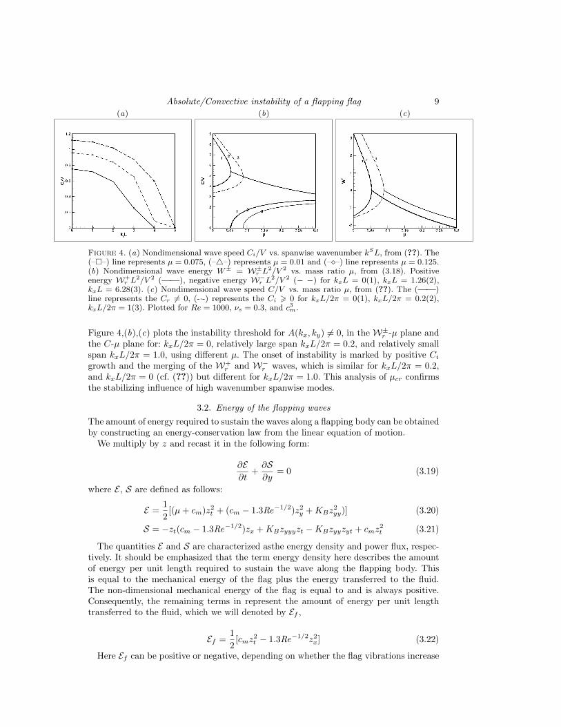
(a) (b) (c)
Figure 4. (a) Nondimensional wave speed Ci/V vs. spanwise wavenumber kSL, from (??). The(–�–) line represents µ = 0.075, (–4–) represents µ = 0.01 and (–�–) line represents µ = 0.125.(b) Nondimensional wave energy W± = W±
r L2/V 2 vs. mass ratio µ, from (3.18). Positive
energy W+r L
2/V 2 (——), negative energy W−r L
2/V 2 (− −) for kxL = 0(1), kxL = 1.26(2),kxL = 6.28(3). (c) Nondimensional wave speed C/V vs. mass ratio µ, from (??). The (——)line represents the Cr 6= 0, (-·-) represents the Ci > 0 for kxL/2π = 0(1), kxL/2π = 0.2(2),kxL/2π = 1(3). Plotted for Re = 1000, νs = 0.3, and c3m.
Figure 4,(b),(c) plots the instability threshold for A(kx, ky) 6= 0, in the W±r -µ plane andthe C-µ plane for: kxL/2π = 0, relatively large span kxL/2π = 0.2, and relatively smallspan kxL/2π = 1.0, using different µ. The onset of instability is marked by positive Ci
growth and the merging of the W+r and W−r waves, which is similar for kxL/2π = 0.2,
and kxL/2π = 0 (cf. (??)) but different for kxL/2π = 1.0. This analysis of µcr confirmsthe stabilizing influence of high wavenumber spanwise modes.
3.2. Energy of the flapping waves
The amount of energy required to sustain the waves along a flapping body can be obtainedby constructing an energy-conservation law from the linear equation of motion.
We multiply by z and recast it in the following form:
∂E∂t
+∂S∂y
= 0 (3.19)
where E , S are defined as follows:
E =1
2[(µ+ cm)z2t + (cm − 1.3Re−1/2)z2y +KBz
2yy)] (3.20)
S = −zt(cm − 1.3Re−1/2)zx +KBzyyyzt −KBzyyzyt + cmz2t (3.21)
The quantities E and S are characterized asthe energy density and power flux, respec-tively. It should be emphasized that the term energy density here describes the amountof energy per unit length required to sustain the wave along the flapping body. Thisis equal to the mechanical energy of the flag plus the energy transferred to the fluid.The non-dimensional mechanical energy of the flag is equal to and is always positive.Consequently, the remaining terms in represent the amount of energy per unit lengthtransferred to the fluid, which we will denoted by Ef ,
Ef =1
2[cmz
2t − 1.3Re−1/2z2x] (3.22)
Here Ef can be positive or negative, depending on whether the flag vibrations increase

10 S. Banerjee and Dick K. P. Yue
Figure 5. Plot of ω vs k for a stable flow [curves (a)], the onset of insta- bility [curves (b)], andan unstable flow [curves (c)]. The shaded parts of the curves correspond to waves with negativeenergy. In curves (a) the positive and negative energy waves do not coalesce, and both solutionsof (3.10) are real; in curves there is a resonance between a positive and a negative energy wavea range of complex frequencies exist, and the waves grow exponentially in time. Only the realpart of the complex ωr is shown.
or decrease the kinetic energy of the fluid. When the latter happens, the flag extractsenergy from the fluid. The power flux on the other hand is equal to minus the power perunit length produced by the internal forces, structural and hydrodynamic, during thelateral vibrations of the flag. For example, represents the power produced by the tensionforce, , the power produced by the bending shear force, and so on.
The average energy of a stable wave of amplitude a0 is given by
E =1
4a20[(µ+ cm)ω2 + (cm − 1.3Re−1/2)k2 +KBk
4)] (3.23)
=1
2a20[(µ+ cm)ω2 − cmkω] (3.24)
= ±1
2a20ωk[−µcm + (µ+ cm)
(1.3Re−1/2 +KBk
2)
]1/2, (3.25)
Thus slow waves, i.e., the waves that correspond to the minus sign in (3.25), carrynegative energy when their frequency is positive. The instability arises when positive andnegative energy waves first coalesce. This is summarized in Fig. 2, where the frequencyω is plotted as a function of the wave number k for three cases: a stable case [curves(a)], where the positive and negative energy waves do not coalesce, and both solutionsof (5) are real; the onset of instability [curves (b)] where there is a resonance betweena positive and a negative energy wave; an unstable case [curves (c)] where a range ofcomplex frequencies exists.
Ef =1
4a20[cmω
2 − 1.3Re−1/2k2] (3.26)
=1
4a20k
2[cmc2p − 1.3Re−1/2], (3.27)

Absolute/Convective instability of a flapping flag 11
(a) (b)
Figure 6. Plot of E± vs k for a stable flow [curves (a)], the onset of insta- bility [curves (b)],and an unstable flow [curves (c)]. The shaded parts of the curves correspond to waves withnegative energy. In curves (a) the positive and negative energy waves do not coalesce, and bothsolutions of (3.10) are real; in curves (b) there is a resonance between a positive and a negativeenergy wave for a range of complex frequencies exist, and the waves grow exponentially in time.Only the real part of the complex ωr is shown.
where cp = ω/k is the phase velocity of the wave. Consequently, Ef becomes negative(which means that the wave extracts energy from the fluid), when the phase velocity ofthe wave is smaller than the free stream velocity. Now, in order for E to become negative,Ef should be negative, but also its magnitude should exceed that of the mechanical(kinetic plus potential) energy of the flag.
From (4) it can be verified that when µ = 0, ω2 is negative for all k; both familiesof waves have then positive energy. It is straightforward to verify that positive values ofω2 appear only when µ exceeds the value specified by (cr). The appearance of negativeenergy waves coincides with the onset of instability. The branch ω2 has negative energyfor k in the range k2 < u ∗ −s. We note that the confirm that slow waves carry negativeenergy as first discussed formally in the study of stability of a two-dimensional flexiblesurface in parallel flow, by ?) and ?).
As we mentioned before, the energy of the waves can become negative when theyextract energy from the fluid.
In order to determine the conditions under which this energy extraction occurs, wesubstitute h = a0 cos(kx− ωt) into (10) and take the average over one wavelength. Thisgives Where c = ω/k is the phase velocity of the wave. Consequently, (Ef ) becomesnegative (which means that the wave extracts energy from the fluid), when the phase-velocity of the wave is smaller than the free stream velocity U. Now, in order for (E) tobecome negative, (Ef) should be negative, but also its magnitude should exceed that ofthe mechanical (kinetic plus potential) energy of the flag. From (4) it is straightforwardto verify that for k < u2s (which is the wave number range over which the branch ω2 hasnegative energy), both branches of the dispersion relation have phase velocities less thanRe. This implies that in this wave number range the negative and the positive energywaves both extract energy from the fluid. The difference between the two is that thelatter extracts an amount less than the mechanical energy of the flag and retains positiveenergy, whereas the former extracts an amount larger than the mechanical energy ofthe flag and acquires negative energy. Both types of waves are stable since they require

12 S. Banerjee and Dick K. P. Yue
Figure 7. Plot of ki vs kr for a stable flow [curves (a)], the onset of instability and an unstableflow. The shaded parts of the curves correspond to waves with negative energy. In curves (a)the positive and negative energy waves do not coalesce, and both solutions of (3.10) are real; incurves there is a resonance between a positive and a negative energy wave a range of complexfrequencies exist, and the waves grow exponentially in time. Only the real part of the complexωr is shown.
either an energy source or an energy sink to be sustained. Instability arises when thetwo types of waves coalesce, since then the negative energy wave provides the energyrequired by the positive energy wave. Consequently, we can anticipate that the energy ofan unstable wave should be zero. In order to verify this, we evaluate the average energyof the unstable flapping waves. Let ω be the real part and ωi the imaginary part of thecomplex frequency of an unstable-wave.
By taking the real and imaginary parts of dispersion relation we find that ω, ωi aregiven by We substitute z = a0 exp(ωit) cos(ky − ωrt), and average over one wavelength.This gives the following result for (E): By substituting it is straightforward to see that(E ) is indeed zero. Thus unstable waves do not require an energy source or an energysink to be sustained. This is due to the fact that the mechanical energy of the flagbecomes equal to the amount of energy extracted from the fluid. Before concluding thissection, we discuss the average power flux associated with the flapping waves. We startwith the stable waves. We substitute z = a0 cos(kx − ωt) into (9) and average overone wavelength to obtain Equation can also be written as Similarily, for the average-energy can be written as It then follows from that, for a stable monochromatic wave,the average energy and average power flux are related through the following expression:where cg is the group velocity The physical interpretation of is that the group velocity isthe velocity of the energy propagation, and is commonly used for the dynamic definitionof the group velocity. We consider next the average-power flux of the unstable waves. Weset into z = a0, exp(ωit) cos(kx − ωrt), average over a wavelength, and obtain or, aftersubstituting into the expressions for ωi, and ωr, we obtain The average-power flux forunstable waves is therefore non- zero, whereas the average energy is zero. Consequently,there is no physically meaningful extension of for unstable waves, and we can concludethat the quantity dω/dk looses its meaning as the velocity of energy propagation.

Absolute/Convective instability of a flapping flag 13
Figure 8. Plot of ωi vs ωr for a stable flow [curves (a)], the onset of instability and an unstableflow. The shaded parts of the curves correspond to waves with negative energy. In curves (a)the positive and negative energy waves do not coalesce, and both solutions of (3.10) are real; incurves there is a resonance between a positive and a negative energy wave a range of complexfrequencies exist, and the waves grow exponentially in time. Only the real part of the complexωr is shown.
3.3. Double Roots
The absolute/convective character of the instability is determined by locating the pinch-ing double roots of the dispersion relation. A pinching double root satisfies the followingequations:
D(ω, k) =∂D
∂k(ω, k) = 0 (3.28)
We set the derivative of the dispersion relation with respect to k equal to zero. Thisgives
∂D
∂k(ω, k) = (cm − 1.3Re−1/2)k − 2KBk
3 − cmω = 0 (3.29)
We solve (3.29) with respect to ω and obtain
ω =(cm − 1.3Re−1/2)k − 2KBk
3
cm= g(k) (3.30)
∆(k) = D(g(k), k) (3.31)
= k2{4(µ+ cm)K2Bk
4 +[3c2mKB − 4KB(µ+ cm)(cm − 1.3Re−1/2)
]k2
+ (µ+ cm)(cm − 1.3Re−1/2)2 − c2m(cm − 1.3Re−1/2)} = 0.
In order to determine the double roots of the dispersion relation, we should solveequation (3.32) with respect to k, then determine ω from (3.30), and see where the latterlies in the upper or lower half of the ω plane. As (3.32) is a fourth-order equation, it canonly be solved numerically. The criterion for absolute instability can however be foundanalytically, without actually solving Eq. (3.32), from the fact, which we will show next,
14 S. Banerjee and Dick K. P. Yue
(a) (b)
(c)
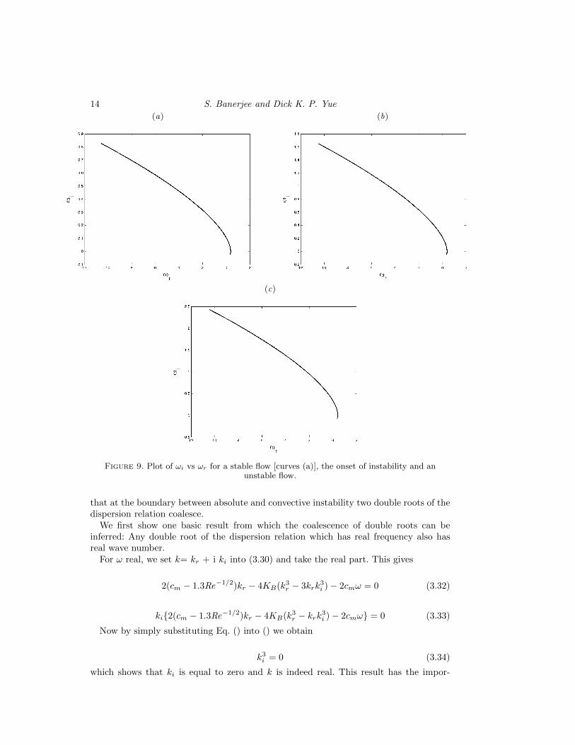
Figure 9. Plot of ωi vs ωr for a stable flow [curves (a)], the onset of instability and anunstable flow.
that at the boundary between absolute and convective instability two double roots of thedispersion relation coalesce.
We first show one basic result from which the coalescence of double roots can beinferred: Any double root of the dispersion relation which has real frequency also hasreal wave number.
For ω real, we set k= kr + i ki into (3.30) and take the real part. This gives
2(cm − 1.3Re−1/2)kr − 4KB(k3r − 3krk3i )− 2cmω = 0 (3.32)
ki{2(cm − 1.3Re−1/2)kr − 4KB(k3r − krk3i )− 2cmω} = 0 (3.33)
Now by simply substituting Eq. () into () we obtain
k3i = 0 (3.34)
which shows that ki is equal to zero and k is indeed real. This result has the impor-

Absolute/Convective instability of a flapping flag 15
tant consequence for different combinations of the parameters µ and Re which lie on theboundary between absolute and convective instability, two double roots of the dispersionrelation coalesce. This can be seen as follows: As the system is nondissipative, the coef-ficients of the dispersion relation are real, and double roots come in complex conjugatepairs. In other words if ω, k is a double root of, so is ω∗, k∗. Consider now the loci of thedouble roots as one, or both, of the parameters µ and Re are varied. When a combinationof µ and Re is approached such that the instability changes from absolute to convective,ω and its complex conjugate ω∗ approach the real axis. At the transition itself, where thefrequency is real, ω and ω∗ become equal. From this we conclude that at the transitionpoints Eq. (3.32) has two equal roots. Equivalently, this implies that at transition
d∆(k)
dk= 0. (3.35)
From (3.32), Eq. (3.40) can be written as
∂D
∂ω
dg
dk+∂D
∂k= 0. (3.36)
As ∂D/∂k, we are left with
∂D
∂ω
dg
dk= 0. (3.37)
In other words, coalescence of two double roots is equivalent with either
D =∂D
∂k=∂D
∂ω=dg
dk= 0. (3.38)
From Eq. (3.30) we have that
dg
dk= −∂
2D
∂k2/∂2D
∂ω∂k. (3.39)
Consequently, (3.38) can be written as
D =∂D
∂k=∂2D
∂k2= 0. (3.40)
3.4. Regions of Absolute and Convective Instability in the µ and Re plane
We now examine the absolute/convective character of the flapping instability. Since themedium is assumed infinitely long, a localized perturbation can either grow in time andspread in space in a way leading to exponential growing motions at any fixed location inspace, or it can grow but at the same time move away from its initial position leading todecaying motions at any fixed location in space. In the first case, the instability is calledabsolute, in the second case it is called convective.
The distinction can be quantified by looking at the Greens function of the system,i.e., the response of Eq. (3.7) to a forcing δ(x)δ(t), where δ(x) stands for the Dirac deltafunction. By taking the Fourier transform of Eq. (3.7) in x, and the Laplace transformin t, the Greens function can be expressed as a double Fourier-Laplace integral following(Bers),
G(x, t) = D(w, k) (3.41)
where k is the Fourier transform variable (wave number), ω is the Laplace transformvariable (frequency), and L, F are integration contours in the complex (w, k) planes,respectively. The long time behavior of the Greens function can be determined by locatingthe pinching double roots of the dispersion relation. Those are defined from

16 S. Banerjee and Dick K. P. Yue
D(ω0, k0) =∂D
∂k(ω0, k0) = 0, (3.42)
plus the pinching requirement that they should result from the coalescence of tworoots corresponding to a left and a right traveling wave. The pinching requirement canbe verified as follows. We consider a vertical line in the com-plex ω plane starting fromthe location of the double root ω and going upwards. We map this line into the complex kplane through the dispersion relation. The mapping will in general have several branches(for the dispersion relation considered here it has four branches). If the branches thatcoalesce at k, originate from different sides of the real axis the double root is of thepinch-point type. If the branches originate from the same side of the real axis, the doubleroot is not of the pinch-point type. In general, double roots will have complex frequenciesand wave numbers. If any pinching double root has a frequency with a positive imaginarypart, then it can be shown that
G(x, t =∞) ∼ (1/√
(t)) exp(i(k0x− ω0t)) (3.43)
The motion grows, therefore, everywherewith a growth rate equal to the imaginarypart of ω0 and the instability is absolute. Otherwise the instability is convective. Thedispersion relation is simple enough for the roots of (23) to be determined analytically.
We differentiate D(ω, k) with respect to k and set the result equal to zero; this gives
k2{4(µ+ cm)K2Bk
4 +[3c2mKB − 4KB(µ+ cm)(cm − 1.3Re−1/2)
]k2 (3.44)
+ (µ+ cm)(cm − 1.3Re−1/2)2 − c2m(cm − 1.3Re−1/2)} = 0.
where Γ is the following expression:
k2{4(µ+ cm)K2Bk
4 +[3c2mKB − 4KB(µ+ cm)(cm − 1.3Re−1/2)
]k2 (3.45)
+ (µ+ cm)(cm − 1.3Re−1/2)2 − c2m(cm − 1.3Re−1/2)} = 0.
It then follows from (25) that all four double roots also have real w. When µ =, Γ =0, and two double roots coalesce to form a third-order root, given by
k2{4(µ+ cm)K2Bk
4 +[3c2mKB − 4KB(µ+ cm)(cm − 1.3Re−1/2)
]k2 (3.46)
+ (µ+ cm)(cm − 1.3Re−1/2)2 − c2m(cm − 1.3Re−1/2)} = 0.
Finally, when µ exits the range defined in (29)) i.e., for
k2{4(µ+ cm)K2Bk
4 +[3c2mKB − 4KB(µ+ cm)(cm − 1.3Re−1/2)
]k2 (3.47)
+ (µ+ cm)(cm − 1.3Re−1/2)2 − c2m(cm − 1.3Re−1/2)} = 0.
Γ becomes complex, yielding double roots with complex k and ω.The loci of the double roots in the complex k and w planes as a function of µ are shown
in Figs. ( cr) and (cr), respectively, for µ =, Re = (only values of µ yielding instabilityare of interest). When (cr) is satisfied double roots with positive ωi exist. These doubleroots satisfy the pinching requirement (see Figs. cr and cr). Consequently, (3.10) is thecondition for absolute instability in the system. When (cr) is satisfied at the transitionfrom convective to absolute instability, the dispersion relation has a third-order root of

Absolute/Convective instability of a flapping flag 17
Figure 10. Plot of ω vs k for a stable flow [curves (a)], the onset of instability and an unstableflow. The shaded parts of the curves correspond to waves with negative energy. In curves (a)the positive and negative energy waves do not coalesce, and both solutions of (3.10) are real; incurves there is a resonance between a positive and a negative energy wave a range of complexfrequencies exist, and the waves grow exponentially in time. Only the real part of the complexωr is shown.
the pinch-point type. The presence of the third-order root in the complex k plane isdemonstrated in Fig. 7. Conditions (cr) also imply that
Equation (cr) is very useful in giving a physical interpretation of the condition forabsolute instability, as it is shown next.
3.5. Spreading of a localized perturbation
Useful insight about the evolution of the instability can be gained by examining the space-time spreading of a localized perturbation. The two ends of a localized perturbation willmove at two characteristic speeds, which we call V1, for the front end, and V2, for theback end.
The instability is then absolute or convective depending on whether V1 and V2, haveopposite signs or the same sign. The two speeds can be determined is as follows:
Consider an observer moving with speed v. The frequency of a wave with respect tothe moving observer, ω′, is given in terms of the frequency of that wave with respectto the stationary observer, ω through a Doppler shift: ω′ + kV = ω. Consequently, thedispersion relation D′(ω′, k) of the moving observer is given by
D′(ω′, k) = D(ω + kV, k). (3.48)
Now if V2 < Rec < V1, the observer moves with the perturbation and his dispersionrelation will indicate an absolute instability; otherwise it will indicate a convective insta-bility. When Rec becomes equal to either V1 or V2, D′(ω′, k) will have a double root onthe ω-real axis. From (cr) we find that D′(ω′, k) is given by
D′(ω′, k) = 0 (3.49)

18 S. Banerjee and Dick K. P. Yue
The dispersion relation of a moving observer D′(ω′, k) is very similar to that of astationary observer (5)) and has also the property that a double root with real frequencyhas real wave number (as it can be formally verified by repeating the dispersion analysis).In other words, when the observer velocity Rec is equal to either V1 or V2, where theinstability changes from absolute to convective, two double roots of the dispersion relationare coalescing. This implies then that V1 and V2, are equal to, respectively, the minimumgroup velocity of the fast waves and the maximum group velocity of the slow wavesin the stationary frame of reference. This is demonstrated in Fig. cr for an absolutelyunstable case, where the dispersion diagram for µ = and Rec =, shows that the extremaof the group velocities have indeed opposite signs. The wave numbers at which the groupvelocity has a minimum or maximum can be found from the condition
This physical interpretation of the absolute/convective character of the instability hasan interesting relation with the amplitude equation of the Kelvin-Helmholtz instability:
Using an argument from operational calculus (i.e. Weissman (1972)) we ex- pand thedispersion relation, for µ−µc, infinitesimal, around (ωc, kc,Rec), and, using Eq. (cr), weobtain
D = 0 (3.50)
where the subscript c implies that the derivative is evaluated at ω = ωc, k = kc, u = uc.The velocities V1, V2 satisfy the following relations, as can readily be verified by directsubstitution:
Now we substitute (51) and (52) into (50), and after replacing (ω − ω0) by id/dt, and(k − k0) by −id/dx, we obtain that the envelope G(x, t) of the wave exp[i(kG−mω, t)]satisfies the unstable Klein-Gordon equation.
D = 0 (3.51)
An initially localized solution of the Klein-Gordon equation (see Bers et al and Huerre)will spread only in one direction if V1V2 > 0, resulting in a convective instability, whereasthe solution will spread in both directions if V1V2 < 0, resulting in an absolute instability,consistently with the result obtained directly from the dispersion relation.
4. Numerical Results
Before we start analyzing the numerical results of the absolute/convective instabilityof a flapping flag, it will be informative to analyze the background research on it, tomotivate the key parameters we use to understand the instability propagation duringflapping.
Kaup et al. (1979) first introduced the local concept of absolutely and convectivelyunstable wave propagation was in the study of plasma instabilities. Huerre & Monkewitz(1985) introduced the following concept in hydrodynamic stability investigations. Fromthese studies we understood that a flow is absolutely unstable if disturbance waves gen-erated by a pulse-wise perturbation (i.e. Dirac delta function in space and time), containamplified upstream and downstream travelling waves, as well as remaining at the loca-tion of its generation, while amplifying in time. The flow is convectively unstable whenthe amplified disturbance waves are convected away from the location of generation suchthat after a sufficiently large time the basic flow is again undisturbed locally. Koch (1985)investigated a family of wake profiles modeled using analytic functions using the localconcept of absolute and convective instability. This was the first study that revealed thatthe wake could be divided into regions of absolute and convective instability delineated

Absolute/Convective instability of a flapping flag 19
the corresponding regions of absolute and convective instability, based on the form ofthe ray diagrams. Gaster (1968) investigated the physical meaning of the singularitiesoccurring in fluid flows, and established their relationship between complex frequenciesand wavenumbers through (dispersion relation) in their study of wake and jet profiles.The local concept of absolute and convective instability analysis can be applied to othershear flows. Huerre & Monkewitz (1985) showed that mixing layers become absolutelyunstable if the two layers propagate in opposite directions with a velocity ratio > 0.136.Following this work, Monkewitz & Sohn (1986) showed that hot jets are absolutely un-stable and Mattingly & Criminale (1972) also suggested from their study of near wakestability that the wake is absolutely unstable. Monkewitz & Nguyen (1987) found thatif the displacement thickness of the boundary layer separating from the body is verysmall, the wake can be first convectively unstable then absolutely unstable and furtherdownstream again convectively unstable for family of wake profiles.
The interesting question discussed by Monkewitz & Nguyen (1987) was whether thereexist a connection between the above-described occurrence of absolute and convectiveinstability in the near wake and the selection of the pure vortex-shedding frequencyobserved in the wake saturation state. These studies led to the classification of the wakefollowing the work of Monkewitz & Sohn (1986) and Triantafyllou et al. (1986) into:AF standing for absolutely unstable with a free boundary that has two transition pointsbetween absolute and convective instability. AB meaning absolutely unstable with a solidboundary having only one transition point, where the absolutely unstable region extendsto the solid boundary of the body. C for completely convectively unstable flow.
We use FSDS to investigate the fully-nonlinear coupled dynamics of the flag flappingproblem. Our objective is to elucidate the behavior of the overall flapping dynamics andits dependence on the relevant nondimensional parameters. Our regime of interest is inthe limit of low bending rigidity (as would be the case of a cloth flag), where the viscoustension dominates the restoring force. As noted in § ??, a finite value of bending rigiditymust be used to ensure robustness of the structural numerical model, and a very lowvalue of bending rigidity of KB = 0.0001 is used in our simulations (the results are notsensitive to variation of KB at this low value).
In addition, we maintain essential inextensibility of the structure using KS = 10.Simulations are initiated with the body straight and at an angle of attack to the flow
such that the initial nondimensional tail amplitude is A0 = 0.1. The initial flow conditionis of a steady uniform flow with a small gradient buffer zone around the body used tominimize transients. As the simulation proceeds the body is initially displaced by thefluid dynamic forcing toward alignment with the incoming flow, and it either settlesto a stable-straight configuration, or experiences sustained flapping. We identify threedistinct regimes of response (dependent on the value of the mass ratio µ): (I) fixed-point stability; (II) limit-cycle flapping; and (III) chaotic flapping. The differences in theresponse among the three regimes can be seen in figure ??, which plots the time history ofthe cross-stream displacement of the trailing edge or tail for one case from each responseregime. In regime (I) the body settles to the steady straight configuration with no cross-stream displacement of the trailing edge, while in regime (II) the response settles to aperiod-one limit-cycle oscillation of constant frequency and amplitude. In regime (III)the trailing edge displacement exhibits sustained non-periodic behavior characteristic ofchaos.
Figure (4, 11) plots the time history of the of cross-stream tail displacement at y/L =1.0 for regime 0.075 6 µ 6 0.350;
For the case of KB = 0.0001 and Re = 1000, we present in figure ?? the results from aseries of simulations through a range of mass ratios of values of µ between 0.025 and 0.3,

20 S. Banerjee and Dick K. P. Yue
(a) (b)
(c) (d)
(e) (f )

Absolute/Convective instability of a flapping flag 21
(g) (h)
(i)
Figure 11. Time history of cross-stream tail displacement at y/L = 1.0 for regime (a) µ = 0.075;(b) µ = 0.125; (c) µ = 0.150; (d) µ = 0.175; (e) µ = 0.200; (f) µ = 0.250; (g) µ = 0.300; (h)µ = 0.325; (i) µ = 0.350 with Re = 1000 and KB = 0.0001.
covering the three response regimes we mentioned. For each mass ratio value, we presentfour plots: a time history of the two-dimensional tail position for twenty nondimensionaltime units; a phase plot of the cross-stream tail displacement against the cross-streamtail velocity; vorticity contours of the flapping wake for the fully developed flow; and afrequency plot displaying the normalized power spectrum for both the cross-stream taildisplacement and the cross-stream flow velocity at a point two body lengths downstreamof the equilibrium tail position.
Figure (4, 12) plots the time history of the of cross-stream tail displacement at y/L =1.0 for regime 0.075 6 µ 6 0.350;
For the regime (I) response for the value of µ = 0.025 (figure ??a), the phase plot

22 S. Banerjee and Dick K. P. Yue
(a) (b)
(c) (d)
(e) (f )
Absolute/Convective instability of a flapping flag 23
(g) (h)
(i)
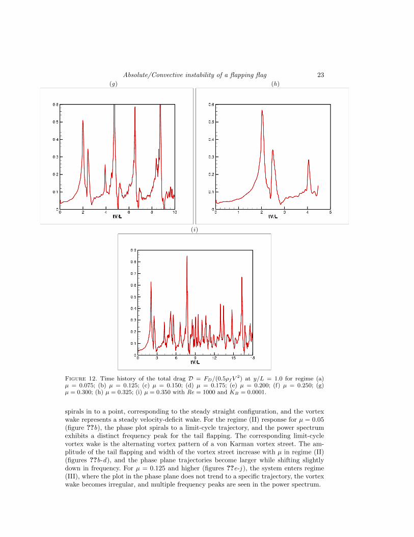
Figure 12. Time history of the total drag D = FD/(0.5ρfV2) at y/L = 1.0 for regime (a)
µ = 0.075; (b) µ = 0.125; (c) µ = 0.150; (d) µ = 0.175; (e) µ = 0.200; (f) µ = 0.250; (g)µ = 0.300; (h) µ = 0.325; (i) µ = 0.350 with Re = 1000 and KB = 0.0001.
spirals in to a point, corresponding to the steady straight configuration, and the vortexwake represents a steady velocity-deficit wake. For the regime (II) response for µ = 0.05(figure ??b), the phase plot spirals to a limit-cycle trajectory, and the power spectrumexhibits a distinct frequency peak for the tail flapping. The corresponding limit-cyclevortex wake is the alternating vortex pattern of a von Karman vortex street. The am-plitude of the tail flapping and width of the vortex street increase with µ in regime (II)(figures ??b-d), and the phase plane trajectories become larger while shifting slightlydown in frequency. For µ = 0.125 and higher (figures ??e-j ), the system enters regime(III), where the plot in the phase plane does not trend to a specific trajectory, the vortexwake becomes irregular, and multiple frequency peaks are seen in the power spectrum.

24 S. Banerjee and Dick K. P. Yue
(a) (b)
(c) (d)
(e) (f )

Absolute/Convective instability of a flapping flag 25
(g) (h)
(i)
Figure 13. Time history of the total lift L = FL/(0.5ρfV2) at y/L = 1.0 for regime (a)
µ = 0.075; (b) µ = 0.125; (c) µ = 0.150; (d) µ = 0.175; (e) µ = 0.200; (f) µ = 0.250; (g)µ = 0.300; (h) µ = 0.325; (i) µ = 0.350 with Re = 1000 and KB = 0.0001.
Figure (4, 13) plots the time history of the of cross-stream tail displacement at y/L =1.0 for regime 0.075 6 µ 6 0.350;
In the following, we discuss details of the fundamental mechanisms associated withthis flapping response and regime transition. We relate the fixed-point stability to thelinear analysis of § ?? and consider the bistable phenomenon observed in prior studies.
Figure (4, 14) plots the time history of the of cross-stream tail displacement at y/L =1.0 for regime 0.075 6 µ 6 0.350;
Figure (4, 15) plots the time history of the of cross-stream tail displacement at y/L =1.0 for regime 0.075 6 µ 6 0.350;

26 S. Banerjee and Dick K. P. Yue
(a) (b)
(c) (d)
(e) (f )

Absolute/Convective instability of a flapping flag 27
(g) (h)
(i)
Figure 14. Time history of the total power P = FP /(0.5ρfV2) at y/L = 1.0 for regime (a)
µ = 0.075; (b) µ = 0.125; (c) µ = 0.150; (d) µ = 0.175; (e) µ = 0.200; (f) µ = 0.250; (g)µ = 0.300; (h) µ = 0.325; (i) µ = 0.350 with Re = 1000 and KB = 0.0001.
Figure (4, 16) plots the time history of the of cross-stream tail displacement at y/L =1.0 for regime 0.075 6 µ 6 0.350;
We also examine the features of the two unsteady flapping regimes and the mechanicsof the transition from limit-cycle to chaotic flapping.
Figure (4, 17) plots the time history of the of cross-stream tail displacement at y/L =1.0 for regime 0.075 6 µ 6 0.350;
28 S. Banerjee and Dick K. P. Yue
(a) (b)
(c) (d)
(e) (f )

Absolute/Convective instability of a flapping flag 29
(g) (h)
(i)
Figure 15. Time history of the total enstrophy |ω2x| at y/L = 1.0 for regime (a) µ = 0.075;
(b) µ = 0.125; (c) µ = 0.150; (d) µ = 0.175; (e) µ = 0.200; (f) µ = 0.250; (g) µ = 0.300; (h)µ = 0.325; (i) µ = 0.350 with Re = 1000 and KB = 0.0001.
5. Conclusions
In the current work the absolute/convective character of the flapping instability of 2Dflag in a uniform flow was investigated. It was first shown that the instability is causedby the coalescence between positive and negative energy waves. Then range of massratios µ leading to an absolute instability was then determined. Regarding the physicalinterpretation of the occurrence of an absolute instability, the criterion as outlined byTriantafyllou & Howell (1994) and Alben (2008) that for unstable waves dω/dk does-notrepresent the group velocity. (Note that the conclusion holds for both growing/decayingwaves.) A better definition of an absolute instability is that the ends of any initially

30 S. Banerjee and Dick K. P. Yue
(a) (b)
(c) (d)
(e) (f )

Absolute/Convective instability of a flapping flag 31
(g) (h)
(i)
Figure 16. Time history of the flag energy budget (ρfV2L2); flag kinetic energy (——), flag
bending energy (—— ), flag extensional energy (—— ) at y/L = 1.0 for regime (a) µ = 0.075;(b) µ = 0.125; (c) µ = 0.150; (d) µ = 0.175; (e) µ = 0.200; (f) µ = 0.250; (g) µ = 0.300; (h)µ = 0.325; (i) µ = 0.350 with Re = 1000 and KB = 0.0001.
localized perturbation will propagate with speeds having opposite signs. In order toobtain a physical interpretation of this definition for any specific problem, one shoulddetermine and physically identify these two characteristic speeds. The main finding thepresent work is that the larger of the two speeds is equal to the minimum group velocityof the fast stable waves, and the smaller of the two speeds is equal to the maximumgroup velocity of the slow stable waves. This property has a direct consequence at theonset of absolute-instability two double roots of the dispersion relation coalesce on thereal axis, forming a third-order root. We find that the absolute/convective character ofthe instability can be inferred from the propagation characteristics of the stable waves in

32 S. Banerjee and Dick K. P. Yue
(a) (b)
(c) (d)
(e) (f )
Absolute/Convective instability of a flapping flag 33
(g) (h)
(i)
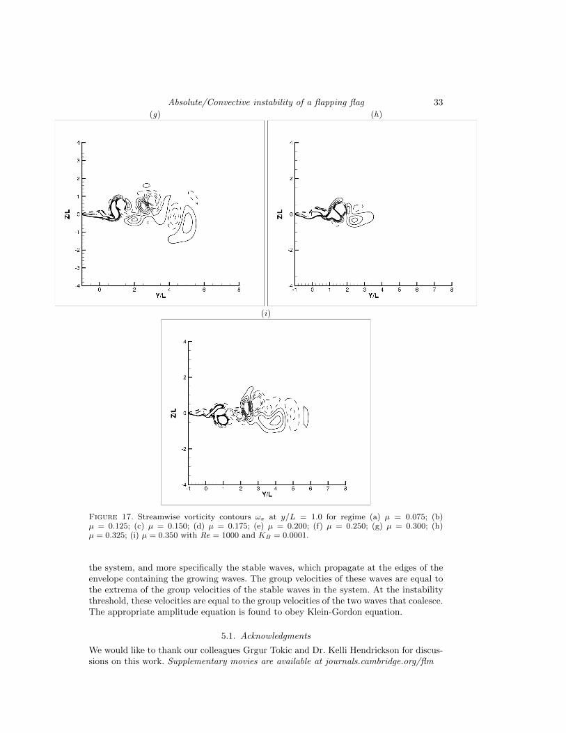
Figure 17. Streamwise vorticity contours ωx at y/L = 1.0 for regime (a) µ = 0.075; (b)µ = 0.125; (c) µ = 0.150; (d) µ = 0.175; (e) µ = 0.200; (f) µ = 0.250; (g) µ = 0.300; (h)µ = 0.325; (i) µ = 0.350 with Re = 1000 and KB = 0.0001.
the system, and more specifically the stable waves, which propagate at the edges of theenvelope containing the growing waves. The group velocities of these waves are equal tothe extrema of the group velocities of the stable waves in the system. At the instabilitythreshold, these velocities are equal to the group velocities of the two waves that coalesce.The appropriate amplitude equation is found to obey Klein-Gordon equation.
5.1. Acknowledgments
We would like to thank our colleagues Grgur Tokic and Dr. Kelli Hendrickson for discus-sions on this work. Supplementary movies are available at journals.cambridge.org/flm

34 S. Banerjee and Dick K. P. Yue
Appendix A. Solver validation
REFERENCES
Alben, S. 2008 The flapping-flag instability as a nonlinear eigenvalue problem. Physics of Fluids20 (10), 104106.
Alben, S. & Shelley, M. 2008 Flapping states of a flag in an inviscid fluid: bistability andthe transition to chaos. Physical review letters 100 (7), 74301.
Argentina, M. & Mahadevan, L. 2005 Fluid-flow-induced flutter of a flag. PNAS 102, 1829–1834.
Benjamin, T. 1963 The threefold classification of unstable disturbances in flexible surfacesbounding inviscid flows. Journal of Fluid Mechanics 16 (03), 436–450.
Brazier-Smith, P. & Scott, J. 1984 Stability of fluid flow in the presence of a compliantsurface. Wave Motion 6 (6), 547–560.
Cairns, R. A. 1979 The role of negative energy waves in some instabilities of parallel flows.J. Fluid Mech. 92, 1–14.
Carpenter, P. & Garrad, A. 1986 Hydrodynamic stability of flow over kramer-type com-pliant surfaces. pt. 2: flow-induced surface instabilities. Journal of Fluid Mechanics 170,199–232.
Coene, R. 1992 Flutter of slender bodies under axial stress. Appl. Sci. Res. 49, 175–187.Connell, B. S. H. 2006 Numerical investigation of the flow-body interaction of thin flexible
foils and ambient flow. PhD thesis, Massachusetts Institute of Technology, Cambridge, MA.Connell, B. S. H. & Yue, D. K. P. 2007 Flapping dynamics of a flag in a uniform stream.
J. Fluid Mech. 581, 33–67.Crighton, D., Oswell, J., Crighton, D. & Oswell, J. 1991 Fluid loading with mean flow. i.
response of an elastic plate to localized excitation. Philosophical Transactions of the RoyalSociety of London. Series A: Physical and Engineering Sciences 335 (1639), 557–592.
Eloy, C., Souilliez, C. & Schouveiler, L. 2007 Flutter of a rectangular plate. J. FluidsStruct. 23, 904–919.
Gaster, M. 1968 Growth of disturbances in both space and time. Physics of Fluids 11 (4),723–727.
Huerre, P. & Monkewitz, P. 1985 Absolute and convective instabilities in free shear layers.Journal of Fluid Mechanics 159, 151–68.
Huerre, P. & Monkewitz, P. 1990 Local and global instabilities in spatially developing flows.Annual Review of Fluid Mechanics 22 (1), 473–537.
Kaup, D., Reiman, A. & Bers, A. 1979 Space-time evolution of nonlinear three-wave in-teractions. i. interaction in a homogeneous medium. Reviews of Modern Physics 51 (2),275.
Koch, W. 1985 Local instability characteristics and frequency determination of self-excitedwake flows. Journal of Sound and vibration 99 (1), 53–83.
Landahl, M. 1962 On the stability of a laminar incompressible boundary layer over a flexiblesurface. Journal of Fluid Mechanics 13 (04), 609–632.
Lucey, A. & Carpenter, P. 1992 A numerical simulation of the interaction of a compliantwall and inviscid flow. Journal of Fluid Mechanics 234 (1), 121–146.
Mattingly, G. & Criminale, W. 1972 The stability of an incompressible two-dimensionalwake. J. Fluid Mech 51 (2), 233–272.
Monkewitz, P. & Nguyen, L. 1987 Absolute instability in the near-wake of two-dimensionalbluff bodies. Journal of fluids and structures 1 (2), 165–184.
Monkewitz, P. & Sohn, K. 1986 Absolute instability in hot jets and their control. In Ther-mophysical Aspects of Re-entry Flows, , vol. 1.
Peake, N. 2003 On the unsteady motion of a long fluid-loaded elastic plate with mean flow.J. Fluid Mech. 507, 335–366.
Shelley, M. J. & Zhang, J. 2011 Flapping and bending bodies interacting with fluid flows.Annu. Rev. Fluid. Mech. 43, 449–465.
Theodorsen, T. & Garrick, I. 1940 Mechanism of flutter: a theoretical and experimentalinvestigation of the flutter problem. National Advisory Committee for Aeronautics.
Absolute/Convective instability of a flapping flag 35
Triantafyllou, G., Triantafyllou, M., Chryssostomidis, C. et al. 1986 On the formationof vortex streets behind stationary cylinders. Journal of Fluid Mechanics 170, 461–77.
Triantafyllou, G. S. 1992 Physical condition for absolute instability in inviscid hydroelsticcoupling. Phys. Fluids 4, 544–552.
Triantafyllou, M. S. & Howell, C. T. 1994 Dynamic response of cables under negativetension: an ill-posed problem. J. Sound Vib. 173, 433–447.
Watanabe, Y., Suzuki, S., Sugihara, M. & Sueoka, Y. 2002 An experimental study ofpaper flutter. J. Fluids Struct. 16, 529–542.
Weissman, M. 1972 Nonlinear development of the kelvin-helmholtz instability. In Proceedings ofthe Washington State University Conference on Mathematical Topics in Stability Theory,March 29-31, 1972 , p. 13. Department of Pure and Applied Mathematics, WashingtonState University.
Zhang, J., Childress, S., Libchaber, A. & Shelley, M. 2000 Flexible filaments in a flowingsoap film as a model for one-dimensional flags in a two-dimensional wind. Nature 408,835–839.
Zhu, L. & Peskin, C. S. 2002 Simulation of flapping flexible filament in a flowing soap film bythe immersed boundary method. J. Comput. Phys. 179, 452–468.
Copyright © 2022 FDOKUMEN