MODELING MATERIALS WITH A STRETCHING THRESHOLD
49
Mathematical Models and Methods in Applied Sciences Vol. 17, No. 11 (2007) 1799–1847 c World Scientific Publishing Company MODELING MATERIALS WITH A STRETCHING THRESHOLD A. FARINA ∗ , A. FASANO and L. FUSI Universit` a degli Studi di Firenze, Dipartimento di Matematica “U. Dini”, Viale Morgagni 67/a, 50134 Firenze, Italy ∗ [email protected]fi.it K. R. RAJAGOPAL Texas A&M University, Department of Mechanical Engineering, College Station, TX 77843, USA [email protected] Received 29 November 2006 Communicated by N. Bellomo We examine the dynamics of materials characterized by the presence of a deformation threshold beyond which no deformation is possible. The class of bodies that we are interested in studying are described by an implicit constitutive relationship between the Cauchy stress and the deformation gradient. A specific one-dimensional dynamical problem is studied, showing that the mathe- matical model takes the form of a hyperbolic free boundary problem in which the free boundary conditions can be of two different types, selected according to whether the stress is continuous at the interface (separating the deformable region from the fully strained region), or whether it is discontinuous. Both situations have been analyzed. Sample numerical computations are carried out using data that are relevant to biologi- cal materials. A comparison with the problem obtained from a limiting procedure for a constitutive model with a piecewise linear elastic response is performed, showing a very interesting feature, namely that the limit does not lead to the solution of the model with a threshold. This is however not surprising as the latter exhibits dissipative behavior. Keywords : Implicit constitutive theories; free boundary problems; wave equations. AMS Subject Classification: 74A99, 35R35, 35L05 1. Introduction Classical models describing the response of continua provide explicit representa- tion for the stress in terms of kinematical variables, e.g., the stress in terms of the linearized strain as in classical linearized elasticity or the stress in terms of the symmetric part the velocity gradient as in the Navier–Stokes fluids. This is also the case of models introduced in linear viscoelasticity by Boltzmann. Noll 1799
Transcript of MODELING MATERIALS WITH A STRETCHING THRESHOLD

November 5, 2007 20:35 WSPC/103-M3AS 00248
Mathematical Models and Methods in Applied SciencesVol. 17, No. 11 (2007) 1799–1847c© World Scientific Publishing Company
MODELING MATERIALS WITH A STRETCHING THRESHOLD
A. FARINA∗, A. FASANO and L. FUSI
Universita degli Studi di Firenze,Dipartimento di Matematica “U. Dini”,
Viale Morgagni 67/a, 50134 Firenze, Italy∗[email protected]
K. R. RAJAGOPAL
Texas A&M University, Department of Mechanical Engineering,College Station, TX 77843, USA
Received 29 November 2006Communicated by N. Bellomo
We examine the dynamics of materials characterized by the presence of a deformationthreshold beyond which no deformation is possible. The class of bodies that we areinterested in studying are described by an implicit constitutive relationship between theCauchy stress and the deformation gradient.
A specific one-dimensional dynamical problem is studied, showing that the mathe-matical model takes the form of a hyperbolic free boundary problem in which the freeboundary conditions can be of two different types, selected according to whether thestress is continuous at the interface (separating the deformable region from the fullystrained region), or whether it is discontinuous. Both situations have been analyzed.Sample numerical computations are carried out using data that are relevant to biologi-cal materials.
A comparison with the problem obtained from a limiting procedure for a constitutivemodel with a piecewise linear elastic response is performed, showing a very interestingfeature, namely that the limit does not lead to the solution of the model with a threshold.This is however not surprising as the latter exhibits dissipative behavior.
Keywords: Implicit constitutive theories; free boundary problems; wave equations.
AMS Subject Classification: 74A99, 35R35, 35L05
1. Introduction
Classical models describing the response of continua provide explicit representa-tion for the stress in terms of kinematical variables, e.g., the stress in terms ofthe linearized strain as in classical linearized elasticity or the stress in terms ofthe symmetric part the velocity gradient as in the Navier–Stokes fluids. This isalso the case of models introduced in linear viscoelasticity by Boltzmann. Noll
1799

November 5, 2007 20:35 WSPC/103-M3AS 00248
1800 A. Farina et al.
(see Ref. 26) introduced the notion of a simple fluid wherein the stress is expressedas a functional of the history of the relative deformation gradient. Such simplefluids include models such as those due to Rivlin and Ericksen21 whose stress ingeneral depends not on more than just one kinematical variable, but rather on atensor (the Rivlin–Ericksen tensor). Also included in the class of simple materialsare the so-called fluids of complexity (m, n) (see Ref. 7) and generalized Newtonianfluids, the power-law fluids being a special subclass of such fluids. There is a funda-mental difference between models such as the classical linearized elastic model andthe linear viscoelastic fluid on the one hand and the Rivlin and Ericksen and thepower-law fluids on the other hand. In the case of the former set of models eitherthe stress can be expressed as a function of the relevant kinematical variables or thekinematical variables can be expressed as a function of the stress (this is also truefor ideal gas law wherein either pressure can be expressed in terms of the specificvolume or vice versa, at constant temperature). However, in the case of generalRivlin–Ericksen fluids or power-law fluids, one cannot express the kinematical vari-able as a function of the stress. In the case of nonlinear elastic solids, given thestress as a nonlinear function of the Cauchy–Green stretch tensor, Truesdell andMoon27 provide sufficient conditions whereby the relationship between the Cauchystress and the stretch can be inverted and the stretch tensor expressed as a functionof stress. Models of both kinds are subclasses of implicit models for elastic bodiesintroduced by Rajagopal.19
Another popular model that has been found to be the most useful in describ-ing the response of many real materials, especially food products, ceramics, waxycrudes, and geological fluids is the Bingham fluid that flows when a certain thresh-old value for the stress is exceeded. If by a “fluid” we mean a body incapable ofresisting a shear stress, the word “fluid” is obviously misused in this case. How-ever, whether a body is a “fluid-like” or “solid-like” is a matter of the time-scaleof observation and the length scales used for measuring the motion and hence it isreasonable to admit models such as the Bingham fluid if the time-scale and lengthscale are appropriate. Once the threshold is exceeded the fluid flows for which a con-stitutive relation is specified. The response of a Bingham fluid, within the contextof one-dimension is depicted in Fig. 1.
We notice that Fig. 1 is a graph and if instead we were to plot shear rate versusthe stress as shown in Fig. 2, we have a functional relationship between the shearrate and the shear stress.
An interesting counterpart to the Bingham fluid-like response is depicted inFig. 4. Such is the response of a spring held in parallel with an inextensibleunstretched string when the stress is expressed as a function of the strain. Onceagain we see that the stress cannot be expressed as a function of the strain whilethe strain can be expressed as a function of the stress.
Both the Bingham fluid and the example shown in Fig. 4 can be viewed aslimiting subclasses of a much more general class of implicit constitutive relations.Let us consider an incompressible fluid whose viscosity depends on the pressure

November 5, 2007 20:35 WSPC/103-M3AS 00248
Modeling Materials with a Stretching Threshold 1801
0
σ
κ
Fig. 1. Shear stress vs. shear rate.
0 σ
κ
Fig. 2. Shear rate vs. shear stress.
in the fluid and the symmetric part of the velocity gradient. In such a fluid onecannot express the stress explicitly in terms of the symmetric part of the velocitygradient (see Refs. 11 and 20). Such models for fluids are not recondite examples;the basic premise in elastohydrodynamics is precisely such an approximation (seeRef. 24). As the fluid is incompressible, the pressure is the mean normal stress andthe viscosity thus depends on the stress, thereby leading to an implicit constitutiverelation between the stress and the symmetric part of the velocity gradient. Asearly as 1889, Barus2 provided an empirical relationship for how viscosity variedwith pressure.

November 5, 2007 20:35 WSPC/103-M3AS 00248
1802 A. Farina et al.
An interesting counterpart to this problem within the context of nonlinear vis-coelastic solids is the constraint of inextensibility (or, in general three dimension, athreshold for the strain tensor) which plays the role that pressure plays in the fluidcase; the constraint could once again be incompressibility or that of inextensibility.
In this paper, we are interested in a case wherein we have a material thathas a threshold for the strain. Until this threshold is reached, the body respondslike an elastic material. In fact, the problem is akin to classical plasticity in thatthe material behaves as an elastic body until a “threshold condition” is reached.However, the similarity with plasticity ends with sharing this notion of an initialelastic response. This problem is in a sense the inverse of “plasticity” in that noflow takes place as the stress is increased beyond the threshold, while in plasticitythere is continued flow even without an increase in stress.
The motion of the “threshold surface” may be entropy producing. This is dueto the fact that the structure of the body changes from being an elastic body toone that cannot be strained further.
Prager15,16 motivated the possibility of response such as that depicted in Fig. 4within the context of the compression of elastic solids and he referred to thephenomenon, wherein after a certain threshold even large increase in stress does notproduce an increase in strain, as “locking.” Such a phenomenon presents itself inthe compression of metallic and polymeric foams and there are several theoreticalas well as experimental papers on this subject. One finds that problems that involveunilateral constraints within the theory of linearized elasticity also leads to similarresponse (see Ref. 5).
The problem studied here is different from these studies on locking as the originalwork of Prager and the subsequent papers on unilateral constraints did not allowfor dissipation and the attendant entropy production. While more recent paperson locking do discuss notions such as damage, there is no rigorous thermodynamicbasis within which such damage is discussed.
While it would be semantically incorrect to think of the material that is respond-ing in an elastic manner and that which is incapable of being strained further astwo phases of a material and the surface that separates them as a phase front, itis instructive to think of the problem to be depicted in such a manner. The “phasetransition” we are talking about is reversible. We then recognize that the movementof the boundary S is akin to the movement of the phase front and in common withsuch a situation we have entropy production (in case of non-vanishing jump of thestress across S) due to the movement of the phase front accompanying the creationof a new phase, in this case the new material that is incapable of further straining.
Tendons, ligaments, tissues are mixtures of inhomogeneous, anisotropic nonlin-early viscoelastic solids and biological fluids. However, to model them as such leadsto mathematical models for complex mixtures that are not amenable to a simpleanalysis. In view of this they are usually modeled as single constituent solid bodies.Of the models that are in vogue, the most common models are those for nonlin-ear elastic and linear viscoelastic solids (see Refs. 8, 12 and 30). In view of the

November 5, 2007 20:35 WSPC/103-M3AS 00248
Modeling Materials with a Stretching Threshold 1803
nonlinear response of most biological materials, it is more common nowadays touse constitutive equations for nonlinear elastic materials. These models are explicitconstitutive equations for the stress. However, the uniaxial extension depicted inFig. 4 has relevance to the uniaxial extension of biomaterials like tendons that arecomposed of elastin (that is spring like) and collagen (that are like strings); thoughthey are not perfectly inextensible since their elastic modulus is quite different fromthat of the elastin.
Elastic solids are usually classified as Cauchy elastic bodies or Green elasticbodies. In the former case the constitutive relation for the stress is given as a func-tion of the deformation gradient, while with regard to the latter class one assumesthe notion of a stored energy which serves as the potential for the Piola–Kirchhoffstress. Recently, it has been shown that the class of materials that have “elasticresponse” is far larger than those that can be categorized as a Cauchy elastic or aGreen elastic body (see Refs. 17 and 18). That such a large class of bodies is pos-sible is a consequence of relaxing a tacit assumption that is made prior to definingeither a Cauchy elastic or Green elastic body, namely that the stress or the storedenergy depends explicitly and only on the deformation gradient. When one givesup this assumption, one finds a much larger class of bodies.
Rajagopal and Srinivasa18 have provided a thermodynamic framework withinwhich to study models that are described by a certain class of implicit constitutiveequations (see Eq. (2.4)). While the stress in such materials cannot be derivedfrom the stored energy, such bodies have a stored energy associated with them.The stored energy however depends on both the stress and the strain. Much moregeneral classes of implicit constitutive relations involving higher time derivatives ofthe stresses and the appropriate kinematic variable are possible (see Ref. 17).
The implicit constitutive equations have been developed recently to describeelastic response are capable of exhibiting an interesting feature that makes themsuitable of describing materials like tendons, namely that of a limit to their extensi-bility. While models to describe limited chain extensibility have been proposed, therelationship between the stress and the kinematical variables are explicit and thestretch tends asymptotically to a limit, i.e., the stress needed to reach this limit isinfinite. On the other hand, implicit models predict that the limit can be reachedwith a finite stress.
There is considerable experimental evidence (see Ref. 13) that indicates thatthe uniaxial response of tendons and ligaments exhibit a pronounced “leg” andconsiderable stiffening on continued extension (see Fig. 3). In the same way asthe one-dimensional Bingham constitutive law can be recovered as a limit caseof power laws (i.e. explicit constitutive laws), one is led to look at the implicitmodel with stretching threshold as the limit of nonlinear elastic models with limitedextensibility. However, we will see that this is not the case, because of the fact thatthe implicit model does not preserve energy in general.
Before proceeding further, it is worth observing that in the one-dimensionalproblem (corresponding to the spring and the inextensible string) that was

November 5, 2007 20:35 WSPC/103-M3AS 00248
1804 A. Farina et al.
introduced, once the one-dimensional body is fully stretched (fully strained) it isnot possible to provide any further stored energy (working) due to its deformation.The body is in fact akin to a rigid body, while its potential and kinetic energy canchange, there can be no change in its energy due to the deformation. We shall seelater that this inability to supply energy has important consequences concerning thedynamics of the “threshold surface” (to be more precise a surface that delineatesthe regions that are capable and incapable of further strain and hence a “strainfront”).
Though we have discussed thus far a problem that has some relevance to thedeformation of biological materials, the three-dimensional version of the problemthat we shall study presents features in common with phenomena occurring ingeological bodies. In many such bodies, which are essentially granular in nature,when sheared, they tend to “lock” after a critical shear is reached. That is, due tothe granular particles re-arranging themselves, they get into a configuration thatdoes not allow any further shearing. Our study is however not directly related tothe deformation of geological bodies as they tend to dissipate energy even before“locking” occurs. Rather, we consider an idealized counterpart wherein before the“locking” the deformation is non-dissipative. In this sense, the problem that westudy is a melding of the one-dimensional problem that we discussed wherein thereis no dissipation until a threshold strain is achieved and the shear problem ofgranular materials wherein “locking” occurs.
We will see that the corresponding mathematical model is a free boundaryproblem for a hyperbolic equation (as expected), in which the free boundary con-ditions may be of two different types, according to whether the velocity field iscontinuous or discontinuous across the interface. The first class, corresponding toa rather artificial set of initial data, produces a subsonic motion of the interface.The natural problem, in which the system is initially at rest and the applied loadreaches and becomes larger than the threshold value, exhibits instead a supersonicinterface. Both situations have been studied, obtaining an existence and unique-ness theorem for the former case, while the latter case is studied for some specificdata, highlighting the typical behavior of the system in the supersonic regime.Numerical results are obtained using biological data for the problem of shearingmotion.
We have also compared the solution to the problem with a stretching thresholdwith the problem in which the constitutive relation for the stress in the strainis piecewise linear, with the slope associated with the second linear relationshiptending in the limit of a sequence of such responses to infinity. We find that the limitof the solution to the second problem does not reproduce the response characteristicof the material with a stretching threshold. The reason for this departure stemsfrom the entropy production due to the dissipation associated with the movingboundary that demarcates the region that has elastic response and that which isincapable of stretching. It is obvious that the body deviates intrinsically from anelastic behavior.
November 5, 2007 20:35 WSPC/103-M3AS 00248
Modeling Materials with a Stretching Threshold 1805
2. The General Model
This section is devoted to the mathematical formulation of the model. After ashort introduction of implicit constitutive models the specific one-dimensional shearproblem is presented.
2.1. Basic definitions
Let us define κR and κt the reference and actual configuration (configuration attime t), respectively, of our body. The motion is described by the mapping χ :(κR ×R) → κt ⊂ R
3, that associates to the pair (X, t) ∈ (κR ×R), representing theparticle labeled by the vector X and the time t, one and only one point x ∈ κt
x = χ(X, t).
We denote by χ−1 the inverse mapping, namely
X = χ−1(x, t).
The velocity and the acceleration of the particle X ∈ κR (at time t) are defined by
v(X, t) =∂χ(X, t)
∂ t,
a(X, t) =∂2χ(X, t)
∂ t2,
respectively. The displacement (at time t) of the particle X with respect to κR isdefined by
u(X, t) = χ(X, t) − X.
We introduce the deformation gradient at (X, t) with respect to κR as the lineartransformation
F = Gradχ(X, t),
where Grad denotes the differentiation with respect to X.We also introduce
L = FF−1 = ∇v, (2.1)
where ∇ denotes the differentiation with respect to the Eulerian coordinates x andthe superposed dot means time differentiation along the particle path.
2.2. Implicit constitutive models
A starting point for implicit constitutive equations for elastic bodies would take theform (see Ref. 17)
g(T,F) = 0, (2.2)

November 5, 2007 20:35 WSPC/103-M3AS 00248
1806 A. Farina et al.
where g is a sufficiently smooth scalar function,a T is the Cauchy stress tensor. Itfollows from frame indifference that the above implicit relationship takes the form:
f(S,E) = 0, (2.3)
where S is the symmetric Piola–Kirchhoff stress, defined throughb
S = det(F)F−1TF−T ,
and E is the Green-St. Venant strain tensor given by
E =12(FT F− I).
When f is continuously differentiable
∂f
∂SS +
∂f
∂EE = 0.
Motivated by this, let us consider the following generalization, namelyc
A(S,E) S + B(S,E) E = 0, (2.4)
where A and B are fourth-order tensors. A relation of the form (2.3), if it is suffi-ciently smooth, will lead to the relation (2.4), but (2.4) is more general in the sensethat not all equations of the form (2.4) can be integrated to obtain (2.3). In thispaper, we shall look at constitutive equations of the form (2.3). It is worth remark-ing that Truesdell25 introduced a class of response functions that is a generalizationof classical elasticity, which he called hypoelastic response. These models are alsoimplicit constitutive relations but do not belong to the class defined above (seeRefs. 3, 4 and 14 for a thermodynamic basis for hypoelastic bodies). Constitutivemodels of the form (2.4) have also been considered before (see e.g., Ref. 10) fordescribing the inelastic response of bodies.
Here we want to model a material in which strain cannot exceed a certain thresh-old. Below that threshold a constitutive law is prescribed as a one-to-one mappingbetween stress and strain, with the stress bounded. Therefore the stretching thresh-old corresponds to the maximal value of stress in the deformability range. Of coursethere will also be a breaking threshold. We suppose that the body is not stressedup to the breaking point.
During the deformation (see Refs. 8 and 30) the body is invariably modeled asa Green elastic solid with the stored energy given in terms of polynomials of theappropriate integrity basis or in terms of an exponential, with the stress being anincreasing function of the strain. The exponential model due to Fung8 allows one tocapture the large variations in the stress σ (σ having the dimension of a pressure,d
[σ] = Pa) due to a relatively small variation in the strain (see Fig. 3).
aIn general g can be also a tensorial function.bThe superscripts “−1” and “−T” stand for the inverse and inverse transpose of the tensor.cWe remark that no analogy can be found between (2.4) and the constitutive laws presented inRefs. 15 and 16.dWith the square brackets we denote the dimension.

November 5, 2007 20:35 WSPC/103-M3AS 00248
Modeling Materials with a Stretching Threshold 1807
Fig. 3. Stress vs. deformation gradient.
We may consider a limiting case of the above behavior assuming (see Fig. 4)that beyond a certain value of the strain, say εo, (or, of the stress, say τ0, [τ0] = Pa)an increase of the applied stress produces no deformation, i.e., the body has become“fully strained” (in the one-dimensional case inextensible). In fact there are severalmodels that are currently used within the context of elasticity that have limitedextensibility, however they tend asymptotically to a limit and the stress is yetexpressed as a function of the strain.
The procedure of considering a sharp threshold as a limiting case of rapidlychanging material properties is ubiquitous in several branches of physics (elastic-plastic and visco-plastic materials, phase change, porous media with no capillarity,infinitely fast chemical reaction, etc.).
Following Rajagopal,17 we consider materials whose response is portrayed inFig. 4. Such a response is possible in bodies characterized by implicit constitutiveequations in which the stress is not derivable from a potential though they have astored energy associated with them. In such bodies the elastic stored energy dependsboth on the deformation gradient F and on the Cauchy stress T. Referring to theone-dimensional case of Fig. 4, the constitutive relation is given by
g(σ, ε) =(
σ − dϕ(ε)dε
)[θ(σ) − θ(σ − τ0)] + θ(σ − τ0)(ε − ε0) = 0, (2.5)
where
θ(σ) =
0, σ < 0,
1, σ ≥ 0,
is the Heaviside function and where ϕ(ε) is a given function such that ϕ′(ε) > 0 forε > 0 and ϕ′(0) = 0.

November 5, 2007 20:35 WSPC/103-M3AS 00248
1808 A. Farina et al.
Fig. 4. Stress vs. deformation gradient. Implicit non-hyperelastic model.
We now show that the constitutive relation (2.5) can be derived from a localdissipation equation which, for isothermal processes, reads ase
T · L − ψ ≥ 0, (2.6)
where:
• T ·L is the stress power.• ψ is the “generalized” stored energy function which may depend on both ε and σ.
We first notice that assuming
ψ(σ, ε) =
ϕ(ε), 0 ≤ σ < τ0,
ψ0 = ϕ(ε0) = const., σ ≥ τ0,(2.7)
and supposing that there exists a surface S ⊂ κt, evolving in time, that separatesthe region where the body is deformable (0 ≤ σ < τ0) from the one where thebody is undeformable (σ ≥ τ0) could be one method of modeling the body. In anydomain that does not contain S, (2.6) can be rewritten as
σ ε − ψ = 0. (2.8)
Indeed, in the unstrained region ε = 0 and, from (2.7) ψ = 0, while in the deformableregion ψ = σ ε.
We now see that locally (avoiding the surface S) (2.8) can be our “constitutiverelation,” i.e., that the constitutive relation (2.5) can be derived from (2.8) and(2.7). Indeed, imposing (2.8) in any region that does not contain S, we have
0 = σ ε − ψ =(
σ − ∂ψ
∂ε
)ε −
(∂ψ
∂σ
),
eRecall that A · B =tr(AT B) = tr(BAT ) = BT · A.

November 5, 2007 20:35 WSPC/103-M3AS 00248
Modeling Materials with a Stretching Threshold 1809
which, because of (2.7), gives
σ =dϕ(ε)
dε, if 0 ≤ σ < τ0, ⇔ 0 ≤ ε < ε0, where ϕ′(ε0) = τ0,
ε = 0,⇒ ε = ε0, if σ ≥ τ0, ⇔ ε ≥ ε0,
or equivalently the implicit relation (2.5).Considering the general 3D case, let us suppose that the constitutive equation is
given by (2.2) (see again Ref. 17). As before, we assume that there exists a surfaceS ⊂ κt, that separates the “deformable region” from the “fully stretched region.” Inother words, denoting by κ
(e)t and κ
(fs)t the region in which the body is deformable
and the one in which deformation has reached the strain threshold, respectively, weassume that
κt = κ(e)t ∪ κ
(fs)t ∪ S and κ1t ∩ κ2t = ∅.
Further, we assume that (2.6) holds true, with “=” in place of “≥,” in any regionthat does not contain S, or, in other words, that dissipation may occur only due tothe movement of S. We also suppose that the “generalized” stored energy functionψ may depend on both T and F, namely
ψ = ψ(T,F).
Differentiating (2.2) along any particle path, avoiding the possible points lying on S,we get (
∂g
∂F(T,F)
)F +
(∂g
∂T(T,F)
)T = 0,
where ∂g∂T and ∂g
∂F are fourth-order tensors. Assuming that ∂g∂T is invertible we obtain
T = h(T,F) F, (2.9)
where h is a fourth-order tensor. From (2.6) we have (recall that the local rate ofdissipation vanishes everywhere inside κ
(e)t and κ
(fs)t )
T · L − ∂ψ
∂F· F − ∂ψ
∂T· T = 0,
which, by virtue of (2.9), entails
T · L − ∂ψ
∂F· F− ∂ψ
∂T· h(T,F) F = 0. (2.10)
From (2.1) F = LF, which substituted into (2.10) yields(T − ∂ψ
∂FFT − hT (T,F)
∂ψ
∂TFT
)· L = 0. (2.11)

November 5, 2007 20:35 WSPC/103-M3AS 00248
1810 A. Farina et al.
Assuming incompressibility, which implies that I · L = 0, we get
T − ∂ψ
∂FFT − hT (T,F)
∂ψ
∂TFT = −φ I, (2.12)
with φ a suitable Lagrange multiplier. When F = I we require that ψ is such that[∂ψ
∂FFT + hT (T,F)
∂ψ
∂TFT
]F=I
= −φ0 I,
consequently we may define the extra stress
Te =∂ψ
∂FFT + hT (T,F)
∂ψ
∂TFT + φ0I, (2.13)
so that Te|F=I = 0. Thus
T = −φ I + Te,
with φ = φ0 + φ. Recently, it has been shown by Rajagopal and Srinivasa18 that(2.13) is a consequence of assuming that the constraint does no work, but that ingeneral, the extra stress can depend on the Lagrange multiplier, a simple exampleof the same being an incompressible viscous fluid whose viscosity is dependent onthe pressure.
Remark 2.1. It has to be noted that, locally (besides S), assuming T · L− ψ = 0does not necessarily mean that globally (i.e., in the whole domain κt) the body doesnot dissipate energy. Indeed, as we shall see in Sec. 2.5, as the surface S moves,entropy may be produced.
2.3. Modeling the stretching threshold
We introduce a function Π which depends on the invariants of Te such that Π = 0when Te = 0. We also introduce a positive threshold Π0, such that the bodybehaves as an elastic body if |Π| < Π0 and that it cannot be deformed if |Π| ≥ Π0.The key point is, of course, the selection of Π, which has to be made on the basisof both experience and experimental results. To be specific we suppose that the“generalized” stored elastic energy per unit volume is given by
ψ =
µ
2tr(B − I), if |Π| < Π0,
ψ0, if |Π| ≥ Π0.(2.14)
where
• [ψ] = J/m3.
• ψ0 ≥ 0.• µ is a positive constant, [µ] = Pa.• B = FFT is the right Cauchy–Green tensor.

November 5, 2007 20:35 WSPC/103-M3AS 00248
Modeling Materials with a Stretching Threshold 1811
We have
∂ψ
∂F=
µF, if |Π| < Π0,
0, if |Π| ≥ Π0,(2.15)
∂ψ
∂T= 0. (2.16)
So, inside the region where |Π| ≥ Π0, (2.11) reduces to
T · L = T ·D = 0, (2.17)
where D =1/2(L + LT ). A possible solution of (2.17) is D = 0. When |Π| < Π0,(2.12) and (2.15) yield
Te = µ(B − I),
and
T = −φI + µB, with φ = µ + φ,
which is the constitutive equation for an incompressible neo-Hookean material.Generally speaking the selection of Π depends on the specific problem under
consideration (it would be different for different materials, say ligaments or tendonsor granular materials that exhibit “locking.” In fact, the three-dimensional modelhas more in common with perfectly smooth elastic granular solids that “lock” thanligaments or tendons as in the three-dimensional body the fibers have a varietyof orientations, i.e., they are anisotropic and that means the response depicted inFig. 4 will not be applicable to the three-dimensional response of such bodies). Asour aim is to merely illustrate the consequence of a threshold for the stretching, weshall make a simple choice and identify Π with ψ
Π =12tr (Te) . (2.18)
2.4. One-dimensional shear problem
Let us consider a homogeneous slab of thickness h loaded on the top surface with aknown shear stress σ, [σ] = Pa. Let x and y be the axes, respectively, parallel andorthogonal to the layers forming the material. We introduce the Lagrangian andEulerian coordinates
X = X e1 + Y e2 + Z e3,
x = xe1 + ye2 + ze3,
and consider a pure shear motionx = X + f (y, t),
y = Y,
z = Z,
⇒
x = X + f (y, t),
y = Y,
z = Z,

November 5, 2007 20:35 WSPC/103-M3AS 00248
1812 A. Farina et al.
f (y, t) being the unknown displacement. Notice that y serves as both a Lagrangianand an Eulerian coordinate.
We assume that the applied shear stress σ takes values greater than τ0 and thatthe surface S separating the region where the body is elastic from that in whichit has reached the maximum strain is, in the (y, t) plane, delineated by the curvey = s(t). So, s(t) is the location of wherein the strain has reached the thresholdvalue at time t. The latter, therefore, is not a material surface. The material isfully strained for s(t) < y ≤ h, i.e., κ
(fs)t ≡ (s, h], and deformable (elastic) for
0 ≤ y < s(t), i.e. κ(e)t ≡ [0, s).
Deformable region, 0 ≤ y < s(t).
The displacement u, written in terms of the Eulerian coordinates, is
u(x, y, z, t) = f (y, t)e1.
Thus velocity and acceleration are given by
v = v(y, t)e1 = ft (y, t) e1,
a = a(y, t)e1 = ftt(y, t)e1.
The deformation gradient and the right Cauchy–Green tensor are
F =
1 fy 0
0 1 0
0 0 1
, B =
1 + f 2y fy 0
fy 1 0
0 0 1
, (2.19)
and the total Cauchy stress tensor is
T =
−φ + µf 2y µfy 0
µfy −φ 0
0 0 −φ
. (2.20)
In particular, denoting by σ the shear stress acting on the layer located at y attime t, we have
σ(y, t) = µfy(y, t),
so that
T =
−φ +σ2
µσ 0
σ −φ 0
0 0 −φ
and Te=
σ2
µσ 0
σ 0 0
0 0 0
.

November 5, 2007 20:35 WSPC/103-M3AS 00248
Modeling Materials with a Stretching Threshold 1813
From (2.18) we have Π = σ2
2µ and we set Π0 = τ20
2µ , since σ (s, t) = τ0 on S. Hence
σ(y, t) ≤ τ0, ∀ y < s (t) , t > 0. (2.21)
We thus requiref
σ(s−, t
) ≤ τ0 ⇔ fy
(s−, t
) ≤ τ0
µ. (2.22)
In particular, recalling (2.14), the “generalized” stored elastic energy (per unitvolume) is
ψ =
µ
2f 2
y , if 0 ≤ |σ| < τ0, (deformable part),
ψ0 =τ20
2µ, if |σ| ≥ τ0, (fully stretched part).
(2.23)
Notice that (2.23) is more akin to a stress based “yield-condition” in plasticity thana strain based “yield criterion.” Concerning the dynamics, writing the equation ofmotion component-wise (and neglecting body forces) we get
ρftt = µfyy − φx, (2.24)
0 = −φy, (2.25)
0 = −φz. (2.26)
Equations (2.25) and (2.26) imply φ = φ(x, t) and Eq. (2.24) becomes
ρftt(y, t) − µfyy(y, t) = −P(t),
with
φx = P(t) =⇒ φ = P(t)x + φ0.
Since we assume that no pressure gradient is applied on the lateral sides of thebody, i.e., P(t) = 0, the equation of motion in the elastic region reduces to
ftt − c2fyy = 0, (2.27)
where
c2 =µ
ρ. (2.28)
The initial data for (2.27) aref(y, 0) = f0(y), 0 ≤ y < s0.
ft(y, 0) = f1(y), 0 ≤ y < s0.(2.29)
Finally, at the bottom surface y = 0 we assume that there is no displacement, i.e.,f(0, t) = 0.
fGiven a generic quantity q(y, t), q(s−, t), and q(s+, t) denote limy→s− q(y, t) and limy→s+ q(y, t),respectively.

November 5, 2007 20:35 WSPC/103-M3AS 00248
1814 A. Farina et al.
Fully strained region. We denote by v(s)(t) the velocity of the fully stretchedregion and by a(s)(t) its acceleration, namely
a(s)(t) =dv(s)(t)
dt, s(t) < y ≤ h.
At the interface y = s(t) we impose continuity of the displacement
f(s+, t) = f(s−, t), (2.30)
which ensures that no ruptures occur. In particular,
f(y, t) = f(s−, t) +τ0
µ(y − s), ∀ y ∈ [s, h] .
since, in the fully stretched region, the strain is uniformly equal to τ0µ . The latter
implies that
v(s)(t) = fy(s−, t)s + ft(s−, t) − τ0
µs, (2.31)
and
a(s)(t) = fyy(s−, t)s2 + 2fyt(s−, t)s + fy(s−, t)s + ftt(s−, t) − τ0
µs. (2.32)
Remark 2.2. (Kinematic jump conditions at the interface) Recalling thatσ(s−, t) = fy(s−, t)/µ (see Fig. 4). We may thus rewrite (2.31) and (2.32) in thefollowing way:
[[v]]S = −τ0 − σ(s−, t)µ
s , (2.33)
[[a]]S = −τ0 − σ(s−, t)µ
s +s
µ
dσ(s−, t)dt
+s
µσt(s−, t), (2.34)
where
[[ (·) ]]S = (·)|y=s+ − (·)|y=s− ,
denotes the jump of the quantity (·) across S.
The Cauchy stress tensor, given by
T =
T11 σ T13
σ T22 T23
T13 T23 T33
,

November 5, 2007 20:35 WSPC/103-M3AS 00248
Modeling Materials with a Stretching Threshold 1815
is independent of x and z because of the assumed form of the motion. Hence T =T(y, t) and T13 = T23 = 0, thus the equations of motion reduce to
ρa(s)(t) = σy. (2.35)
Imposing the boundary condition T(h, t)e2 = σ(t)e1 on y = h we get
σ(y, t) = ρa(s)(t) (y − h) + σ(t). (2.36)
Obviously, σ(y, t) ≥ τ0, ∀ y ≥ s(t), thus
σ(s+, t) ≥ τ0. (2.37)
Remark 2.3. (Dynamic jump conditions at the interface) Considering the entiredomain
D =(y, t) ∈ R
2 : 0 < y < h, 0 < t < T
, T > 0, (2.38)
and
S =(y, t) ∈ R
2 : y = s (t) , 0 ≤ t < T
,
the conservation of the linear momentum in D can be rewritten as
ρ vt + ρ[[v]]Sδ (S)nS · et = σy + [[σ]]Sδ (S)nS · ey , (2.39)
where
• vt and σy denote the piecewise continuous “part” of ∂σ/∂y and ∂v/∂t, i.e.,the classical derivative of σ and v in D\S (see, for instance, Ref. 28, Sec. 6).
• δ(S), denotes the Dirac delta “centered” along the curve S.• nS is the normal to S
nS =1√
1 + s2(ey − set) . (2.40)
In particular, (2.39) entails the usual jump relation for the linear momentum
ρ[[v]]S s = −[[σ]]S , (2.41)
(see also Ref. 6, Chap. 8), which can also be deduced combining the linear momen-tum balance applied to the whole system and the one applied only to the fullystretched region.
Dynamics of the interface S. We consider a domain
Ω = x0 < x < x0 + 1, z0 < z < z0 + 1, < y < h,

November 5, 2007 20:35 WSPC/103-M3AS 00248
1816 A. Farina et al.
for some x0, z0, s(t) < < h at a given time t and, in the same spirit of Ref. 29,p. 90, we apply the conservation of linear momentum thereby obtaining
d
dt
[ρv(s)(t)(h − )
]= σ − σ(, t), (2.42)
since σ(t) − σ(, t) is the resultant of all external forces (parallel to e1) acting onΩ. If after differentiation we take the limit → s(t)+ we get
ρ a(s)(t)(h − s) = σ − σ(s+, t), (2.43)
which coincides with the limit y → s+ of (2.36) and has to be coupled with theinitial condition
v(s)(0) = v(s)0 .
Moreover, we suppose that, if at t = 0 the fully strained region is present, we havethe compatibility condition
v(s)0 =
(f ′0 (s0) − τ0
µ
)s(0) + f1 (s0) . (2.44)
Remark 2.4. In deriving (2.43), we could have selected smaller than s(t), i.e.0 < < s(t), so that Ω ∩ 0 < y < s = ∅. In such a case, denoting by P the linearmomentum of Ω, namely
P (t) =∫ h
ρv(y, t)dy =∫ s
ρv(y, t)dy + ρ (h − s) v(s) (t) ,
we have
P (t) =∫ s
ρvt(y, t)dy − ρ[[v]]S s + ρ (h − s) a(s)(t).
On the other hand
P (t) = σ − σ(, t),
so, exploiting (2.27) and (2.41), we get
σ − σ(, t) = σ(s−, t
)− σ(, t) + [[σ]]S + ρa(s)(t) (h − s) ,
that is (2.43).
Concerning the stress σ(s+, t) which appears in the R.H.S. of (2.43), it can beexpressed in terms of σ(s−, t), exploiting both (2.33) and (2.41). Indeed, from them

November 5, 2007 20:35 WSPC/103-M3AS 00248
Modeling Materials with a Stretching Threshold 1817
we obtain
σ(s+, t) = σ(s−, t) +s2
c2
(τ0 − σ(s−, t)
), (2.45)
so that (2.43) reads
ρ a(s)(t)(h − s) = σ −[σ(s−, t) +
s2
c2(τ0 − σ(s−, t))
]. (2.46)
Finally, using (2.32) and recalling that σ(s−, t) = µ fy(s−, t), we derive the freeboundary condition[
(h − s)(
fy − τ0
µ
)s +
((h − s)fyy +
τ0
µ− fy
)s2
+ 2(h− s)fyts + (h − s)ftt + c2fy
]y=s−
=σ
ρ, (2.47)
which has to be coupled with the initial conditionss(0) = s0, 0 ≤ s0 ≤ h,
s2(0)c2
(τ0 − σ(s−0 , 0)) = [[σ]]S |t=0.(2.48)
The free boundary problem. We are now in the position to express the generalmodel in the deformable region as a hyperbolic free boundary problem.
ftt − c2fyy = 0,0 < y < s(t),
t > 0,
f(0, t) = 0, t > 0,
fy(s(t), t) =σ(s−, t)
µ, with σ(s−, t) ≤ τ0, t > 0,[
(h − s)(
fy − τ0
µ
)s +
((h − s)fyy +
τ0
µ− fy
)s2
+ 2(h− s)fyts + (h − s)ftt + c2fy
]y=s−
=σ
ρ, t > 0,
f(y, 0) = f0(y), 0 ≤ y ≤ s0,
ft(y, 0) = f1(y), 0 ≤ y ≤ s0,
s(0) = s0, 0 ≤ s0 ≤ h,
s2(0)c2
(τ0 − σ(s−0 , 0)) = [[σ]]S |t=0,
(2.49)
where f0(y) must be such that f ′0(y) ≤ τ0/µ, ∀ y ≤ s0.

November 5, 2007 20:35 WSPC/103-M3AS 00248
1818 A. Farina et al.
We notice that in (2.49) one condition is still missing since the system containsthe extra unknown σ(s−, t). Indeed retrieving the missing condition is an intrinsicdifficulty of this problem which makes it quite peculiar. As we shall see, it turnsout that, depending on the initial and boundary data, the problem itself selectsthe additional information which is required to close the system. This depend onwhether [[σ]]S = 0 or [[σ]]S > 0. We can now prove the following:
Proposition 2.1. Let (f, s, σ) be a solution of problem (2.49) in D given by (2.38)and σ(t) > τ0, for some t ≥ 0, then:
1. If |s| < c, then [[σ]]S = 0 (there is no jump of the stress across the interface).2. If |s| = c, then σ(s+, t) = τ0 (and thus [[σ]]S ≥ 0).3. If |s| > c, then either σ(s−, t) = τ0 = σ(s+, t) (i.e. [[σ]]S = 0) or σ(s−, t) < τ0 <
σ(s+, t).4. If [[σ]]S = 0, i.e., σ(s−, t) = σ(s+, t) = τ0, then relation (2.45) is identically
satisfied irrespectively of s.5. If [[σ]]S > 0, then [[v]]S = 0(if s = 0) and τ0 > σ(s−, t). The physical requirement
(2.37) can be fulfilled only if
|s| ≥ c,
(a jump in the stress).
Proof. Equation (2.45) may be rewritten as
σ(s+, t) − τ0 = (τ0 − σ(s−, t))(
s2
c2− 1
), (2.50)
from which all the results follow immediately.In particular, concerning point 5, [[v]]S = 0 with s = 0 is a consequence of (2.41)
and τ0 > σ(s−, t) because of (2.33).
When the stress is continuous across S, namely σ(s−, t) ≡ τ0 ≡ σ(s+, t), (2.49)3and (2.49)4 reduce to
fy(s(t), t) =τ0
µ, (2.51)
[fty(s−, t) s + c2fyy(s−, t)
](h − s) =
σ − τ0
ρ, (2.52)
respectively.On the other hand, if in the time interval considered [[σ]]S > 0 (which leads to
|s| ≥ c, as seen in Proposition 2.1) f(y, t) is essentially determined by the initialdata via d’Alembert formula (in other words, problem (2.49)1, (2.49)2, (2.49)5, and(2.49)6 can be solved autonomously) so that Eq. (2.49)3 can be used to evaluateσ(s−, t).

November 5, 2007 20:35 WSPC/103-M3AS 00248
Modeling Materials with a Stretching Threshold 1819
Remark 2.5. If we compute the time derivative of the linear momentum for thewhole layer we find that
d
dt
(∫ h
0
ρv dy
)= ρ
∫ s
0
ftt(y, t)dy + [[σ]]s + ρ (h − s) a(s)(t) = −µfy(0, t) + σ,
where (2.27), (2.39) and (2.43) have been exploited. Thus −µfy(0, t) is the reactiondue to the constraint on y = 0.
2.5. Energy considerations and dissipation
We introduce the total kinetic energy
K =∫ h
0
12ρv2dy,
and the total stored energy
Ψ =∫ h
0
ψdy,
with ψ given by (2.23), i.e.
Ψ =∫ s
0
µ
2f 2
y dy +∫ h
s
τ20
2µdy or Ψ =
∫ s
0
σ2(y, t)2µ
dy +∫ h
s
τ20
2µdy. (2.53)
The global energy balance for the system can be written as (see, for instance, Ref. 6,Chap. 7, Secs. 2 and 3.1)
d
dt(K + Ψ) = Pext − Pdiss, (2.54)
where Pext is the power exerted by external forces, namely
Pext = σ v (h, t) = σ v(s)(t),
and Pdiss denotes the global power dissipated.
Proposition 2.2. Energy is dissipated if and only if s < 0 and σ(s+, t) > τ0. Moreprecisely, the dissipated energy is given by
Pdiss =[[v]]S
2(σ(s+, t) − τ0
). (2.55)
Moreover Pdiss is necessarily non-negative and Pdiss > 0 is compatible only withs < 0 and σ(s+, t) > τ0 (in other words a regression of the fully strained regioncannot lead to dissipation and requires σ(s+, t) = τ0).

November 5, 2007 20:35 WSPC/103-M3AS 00248
1820 A. Farina et al.
Proof. Let us now evaluate explicitly K and Ψ. Considering first K, we have
dK
dt=
d
dt
(∫ s
0
12ρ v(y, t)2dy +
∫ h
s
12ρ v(s)(t)2dy
)
=∫ s
0
ρ v vtdy︸ ︷︷ ︸Rs0 vσy dy
+∫ h
s
ρv(s)a(s)dy︸ ︷︷ ︸R hs
v(s) σydy=v(s)R h
sσydy
−ρ
2[[v2]]S s
=∫ s
0
((vσ)y − vyσ )dy︸ ︷︷ ︸σ(s−,t)v(s−,t)−R
s0 vyσ dy
+ σ v(s)(t)︸ ︷︷ ︸Pext
−σ(s+, t)v(s)(t) − ρ
2[[v2]]S s ,
yielding
dK
dt= Pext −
∫ s
0
σvydy − ρ
2[[v2]]S s − [[σ v]]S . (2.56)
Next, concerning Ψ, using the second expression recorded in (2.53), we have
dΨdt
=∫ s
0
σ
µσtdy︸ ︷︷ ︸R s
0 µfy fyt dy
−(
τ20
2µ− σ(s−, t)2
2µ
)s
=∫ s
0
σvydy − 12µ
(τ20 − σ(s−, t)2
)s . (2.57)
If we now substitute (2.56) and (2.57) into (2.54) we obtain the following generalexpression for Pdiss,
Pdiss = [[σ v]]S + s
[12µ
(τ20 − σ(s−, t)2
)+
ρ
2[[v2]]S
]. (2.58)
The R.H.S. of (2.58) can be expressed in a more compact form. Indeed, from (2.41),after some algebra, we get
[[σv]]S +12ρ s[[v2]]S =
σ(s+, t) + σ(s−, t)2
[[v]]S .
Thus, the R.H.S. of (2.58) can be rewritten as
σ(s+, t) + σ(s−, t)2
[[v]]S +s
2µ
(τ20 − σ2(s−, t)
),

November 5, 2007 20:35 WSPC/103-M3AS 00248
Modeling Materials with a Stretching Threshold 1821
which, exploiting (2.45) and (2.41), reduces to
[[v]]S2
(σ(s+, t
)− τ0
).
So, formula (2.55) is proved.Concerning the second point of the proposition, we first rewrite (2.55) in a form
involving s explicitly. Using (2.41) we obtain this fairly simple expression
Pdiss =[[σ]]S2ρ s
(τ0 − σ(s+, t)
). (2.59)
So, Pdiss = 0 if and only ifg τ0 = σ(s+, t).Let us now show that Pdiss is nonnegative. Indeed, introducing the total entropy
S, the global form of the Clausius–Duhem inequality (systems at uniform constanttemperature) is
dS
dt+
Q
θ≥ 0,
with θ absolute temperature and Q total heat exchanged with the exterior. Now,in isothermal problems involving elastic solids, it is commonly assumed thath
θS = E − Ψ,
with E total internal energy. Hence
d (Sθ)dt
+ Q =dE
dt− dΨ
dt+ Q =
d (E + K)dt︸ ︷︷ ︸
Pext−Q
− d (Ψ + K)dt︸ ︷︷ ︸
Pext−Pdiss
+ Q = Pdiss,
where we have used (2.54) and the first principle of thermodynamics. We thereforeconclude
Pdiss ≥ 0. (2.60)
So, from (2.59) we have
[[σ]]S2ρ s
(τ0 − σ(s+, t)
) ≥ 0, (2.61)
that requires s < 0, since [[σ]]S(τ0 − σ(s+, t)) ≤ 0. If energy dissipation occurs thenthe fully strained region is expanding. In other words, the shrinking of the fullystretched region (i.e. s > 0) is only compatible with σ(s+, t) = τ0.
It can be easily seen that in any region that does not contain the interface S, thelocal rate of dissipation vanishes. Such a result (consistent with our constitutiveprocedure) does not apply to the global domain. This fact indicates the productionof entropy due to the motion of S.
gRecall that τ0 = σ(s+, t) does not imply, in general, [[σ]]S = 0, while [[σ]]S = 0 implies τ0 =σ(s+, t).hSuch an assumption is tantamount to requiring that the Helmholtz free energy coincides withthe total stored elastic energy Ψ.

November 5, 2007 20:35 WSPC/103-M3AS 00248
1822 A. Farina et al.
2.6. The mathematical problem
Going back to Sec. 2.4, we consider the transformation (see Ref. 9)
w(y, t) = fy(y, t), (2.62)
whose inverse is given by
f(y, t) =∫ y
0
w(ξ, t)dξ. (2.63)
Introducingi
w0(y) = f ′0(y) and w1(y) = f ′
1(y),
problem (2.49) is transformed towtt − c2wyy = 0, 0 < y < s(t), t > 0,
wy(0, t) = 0, t > 0,
w(y, 0) = w0(y), 0 ≤ y ≤ s0,
wt(y, 0) = w1(y), 0 ≤ y ≤ s0,
(2.64)
to which, according to whether [[σ]]S ≡ 0 or not, we have to add:
• [[σ]]S ≡ 0, w(s, t) =
τ0
µ, t > 0,
(h − s)[wt s + c2wy
]y=s− =
σ − τ0
ρ, t > 0,
s(0) = s0, 0 ≤ s0 ≤ h.
(2.65)
• [[σ]]S = 0,
w(s(t), t) =σ(s−, t)
µ, with σ(s−, t) ≤ τ0, t > 0,[
(h − s)(
w − τ0
µ
)s +
((h − s)wy +
τ0
µ− w
)s2
+ 2(h− s)wts + c2(h − s)wy + c2w
]y=s−
=σ
ρ, t > 0
s(0) = s0, 0 ≤ s0 ≤ h.
s2(0)c2
(τ0 − σ
(s−0 , 0
))= [[σ]]S |t=0.
(2.66)
Before studying this problem we cast it into a non-dimensional form. We rescalethe independent variables as follows:
y = hy, t =h
ct.
iRecall that (2.21) implies w0(y) ≤ τ0/µ ∀ 0 ≤ y ≤ s0.

November 5, 2007 20:35 WSPC/103-M3AS 00248
Modeling Materials with a Stretching Threshold 1823
We also definej
w(y, t
)= w
(hy,
h
ct
), w0 (y) = w0 (hy) , w1 (y) =
h
cw1 (hy) ,
and
a(s)(t)
=c2
ha(s)
(h
ct
), s(t) =
s(t)h
, s0 =s0
h.
Problem (2.64) with (2.65) or (2.66), becomeswtt − wyy = 0, 0 < y < s
(t), t > 0,
wy
(0, t
)= 0, t > 0,
w (y, 0) = w0 (y) , 0 < y < s0,
wt (y, 0) = w1 (y) , 0 < y < s0,
(2.67)
and
• [[σ]]S ≡ 0, w
(s, t
)=
τ0
µ, t > 0, ,
(1 − s )[wt
˜s + wy
]y=s− =
σ − τ0
µ, t > 0,
s(0) = s0, 0 ≤ s0 ≤ 1.
(2.68)
• [[σ]]S = 0,
w(s, t
)=
σ(s−, t
)µ
, with σ(s−, t
) ≤ τ0, t > 0,[(1 − s)
(w − τ0
µ
)˜s +
((1 − s) wy +
τ0
µ− w
)˜s2
+ 2 (1 − s) wt˜s + (1 − s) wy + w
]y=s−
=σ
µ, t > 0,
s(0) = s0, 0 ≤ s0 ≤ 1,
˜s2(0)
(τ0 − σ
(s−0 , 0
))= [[σ]]S |t=0 .
(2.69)
Here and in the sequel, to simplify the notation, we will omit the “tildas.” Wefinally remark that σ, σ, τ0, and µ keep their dimensions (i.e. Pa). The expressionsτ0µ and bσ
µ (which appear in (2.68), (2.69) and in later formulas) are dimensionless.
jNotice that w = ∂ f∂y
where f = h−1f .

November 5, 2007 20:35 WSPC/103-M3AS 00248
1824 A. Farina et al.
3. Analytical Results when [[σ]]S ≡ 0
In this section we show existence and uniqueness of a solution to problem (2.67),(2.68) when [[σ]]S ≡ 0 (i.e. σ(s−, t) = τ0). As we shall see, the corresponding situa-tion is rather artificial from a physical point of view, since very peculiar conditionsmust be imposed on the data. Besides f0, f1 ∈ C2, we consider
T < min s0, 1 − s0 . (3.1)
and we will assume the following hypotheses:
H.1 0 < s0 < 1 and the initial velocity of the fully strained part is given by (2.44).H.2 Extending the initial data w0(y) and w1(y) as even functions in [−s0, 0], there
exist two positive constants W1 and W2, such that
W1 ≤ w′0(y) − w1(y) ≤ W2, for all y ∈ [−s0, s0].
H.3 Further w0(y) and w1(y) meet the following conditions:w0(s0) =
τ0
µ,
w′0(s0) = 0,
w′0(0) = 0.
(3.2)
Notice that H.2, (3.2)2, and (3.2)3 imply W1 ≤ −w1(0) ≤ W2, W1 ≤ −w1(s0) ≤W2. In particular, the former, because f = 0 on y = 0, implies that the initialvelocity is negative in a neighborhood of y = 0.
H.4 Introducing
K(t) =σ(t) − τ0
µ, (3.3)
we assume that supt∈[0,T ] K(t)2 (1 − s0)W1
< 1,
inf t∈[0,T ] K(t)W2
> 1,
(3.4)
requiring the compatibility condition W2 < 2(1 − s0)W1.
3.1. Local qualitative analysis
Assuming for the moment that the problem defined through (2.67) and (2.68) has asolution and that −1 < s(t) < 1 for t ∈ [0, T ] (in physical terms the free boundaryvelocity is less than c), we consider the domains (see Fig. 5)
Ds, T =(y, t) ∈ R
2 : 0 < y < s(t), 0 < t < T
,
D(I)s, T = (y, t) ∈ Ds, T : 0 < y < s0 − t, 0 < t < T ,
D(II)s, T = (y, t) ∈ Ds, T : s0 − t < y < s(t), 0 < t < T ,

November 5, 2007 20:35 WSPC/103-M3AS 00248
Modeling Materials with a Stretching Threshold 1825
Fig. 5. The domains D(I)s, T and D
(II)s, T . Time T satisfies (3.1).
with T fulfilling (3.1). Of course
Ds, T = D(I)s, T ∪ D
(II)s, T .
We can give a representation formula for w in terms of the initial and bound-ary data. Indeed, exploiting the results documented in Ref. 9 the solution of thehyperbolic equation is given by the formula
w(y, t) =
12
[w0 (y − t) + w0 (y + t)] +12
∫ y+t
y−t
w1 (ξ) dξ, if (y, t) ∈ D(I)s, T ,
τ0
µ+
12
[w0 (y − t) − w0 (s (t∗) − t∗)]
+12
∫ s(t∗)−t∗
y−t
w1 (ξ) dξ, if (y, t) ∈ D(II)s, T
(3.5)
where, as mentioned, the initial data w0(y) and w1(y) have to be extended as evenfunctions in [−s0, 0] and where t∗ = t∗(y, t) is the unique solution of the implicitequation
s(t∗) + t∗ = y + t. (3.6)
In practice t∗(y, t) < t is the time at which the characteristic coming from(y, t), with slope −1, meets the free boundary. The condition |s| < 1, ∀ t ∈ [0, T ],guarantees the existence and uniqueness of t∗.
Formula (3.5) allows one to evaluate explicitly wy , wt, wyy, and wtt (see Ref. 9,Sec. 4.3), whose expressions involve s and s. Thus the regularity of w depends on

November 5, 2007 20:35 WSPC/103-M3AS 00248
1826 A. Farina et al.
Fig. 6. Intersection between the characteristic and the free boundary.
the regularity of s. In particular, if s(t) ∈ C[0, T ] with s(t) ∈ L∞(0, t) and |s| < 1,we may verify that w(y, t) ∈ C(Ds,T ), provided w0(s0) = τ0
µ .From (3.6) we have
∂t∗
∂y=
∂t∗
∂t=
1s(t∗) + 1
,
thus, on exploiting (3.5), we obtain that
wy(y, t) =
12
[w′0 (y − t) + w′
0 (y + t)]
+12
[w1 (y + t) − w1(y − t)] , if (y, t) ∈ D(I)s, T ,
12
[w′
0 (y − t) − w′0 (s (t∗) − t∗)
s(t∗) − 1s(t∗) + 1
]+
12
[w1 (s (t∗) − t∗)
s(t∗) − 1s(t∗) + 1
− w1(y − t)]
, if (y, t) ∈ D(II)s, T ,
(3.7)
wt(y, t) =
12
[w′0 (y + t) − w′
0(y − t)]
+12
[w1 (y + t) + w1(y − t)] , if (y, t) ∈ D(I)s, T ,
−12
[w′
0 (y − t) + w′0 (s (t∗) − t∗)
s(t∗) − 1s(t∗) + 1
]
+12
[w1(y − t) + w1 (s (t∗) − t∗)
s(t∗) − 1s(t∗) + 1
], if (y, t) ∈ D
(II)s, T .
(3.8)

November 5, 2007 20:35 WSPC/103-M3AS 00248
Modeling Materials with a Stretching Threshold 1827
Remark 3.1. If we evaluate the derivative of w along the characteristics
Σα : y + t = α, with 0 ≤ α ,
we obtain, by virtue of (3.7), (3.8) and assumption H.2,
d
dt(w|Σα ) = −wy (Σα) + wt (Σα)
= − (w′0(α − 2t) − w1(α − 2t)) < 0. (3.9)
Thus, recalling (3.2), the above means that w remains below τ0/µ in thedomain Ds, T .
Proposition 3.1. Let H.1–H.4 hold true. Then a time θ can be computed suchthat a unique solution (w, s, σ) to problem (2.67), (2.68) exists for t ∈ [0, θ), withthe property −1 < s < 0 (hence [[σ]]S ≡ 0).
Proof. We observe that [[v(t = 0)]]S ≡ 0 (from H.1) implies [[σ(t = 0)]]S ≡ 0because of (2.41), allowing, by means of (2.46), the computation of
a(s)(0) =K(0)1 − s0
.
On the other hand, from (2.32) we get the expression
a(s)(0) = w′0 (s0)
(1 + s2(0)
)︸ ︷︷ ︸ + 2s(0)w1 (s0) ,
=0
by (3.2)2
thus concluding that
s(0) =a(s)(0)
2w1 (s0)=
K(0)2w1 (s0) (1 − s0)
> − supt∈[0,T ] K(t)2 (1 − s0)W1
,
which by virtue of H.2 and (3.4)1 implies that any solution of problem (2.67) mustsatisfy
−1 < s(0) < 0.
At this point we try to construct a solution in some time interval (0, θ) withthe property −1 < s < 0, which, by Proposition 2.1, is characterized by [[σ]]S ≡ 0.The corresponding free boundary conditions are (2.68). Differentiating (2.68)1 weobtain wt(s, t) + swy(s, t) = 0, allowing one to eliminate wt in (2.68)2
wy (s, t)(1 − s2
)(1 − s) = K. (3.10)
Having computed wy explicitly (see (3.7) when y = s(t) ⇒ t∗ = t) we may refor-mulate (3.10) as a first-order nonlinear ODE for s(t)
s = 1 −F (s, t) ,
s(0) = s0,(3.11)

November 5, 2007 20:35 WSPC/103-M3AS 00248
1828 A. Farina et al.
with
F (s, t) =K(t)
(1 − s) [w′0(s − t) − w1(s − t)]
. (3.12)
Now we prove that the condition (3.4)2 allows to construct a solution to problem(2.67), (2.68) with the desired properties in some interval (0, θ), which can be easilyestimated. Indeed, from H.2, H.4 and (3.12) we get
s > 1 − K(t)(1 − s)W1
> 1 − 21 − s0
1 − s, (3.13)
and if we want s > −1 we may require 1−s01−s < 1, which is in turn guaranteed by
s < 0. The latter condition is equivalent to F(s, t) > 1, that is implied by (3.4)2.From (3.13) we deduce that
(1 − s) s > − [1 − s0 − (s0 − s)] , (3.14)
and require
1 − s0 − (s0 − s) > 0, i.e.s0 − s
1 − s0< 1.
The differential inequality (3.14), for s0−s1−s < 1, can be rewritten as
1 − s
1 − s0 − (s0 − s)s > −1 ⇒
(−1 +
21 − s0−s
1−s0
)s > −1
which, when integrated, gives
−
s0 − s
1 − s0− 2 ln
(1 − s0 − s
1 − s0
)> − t
1 − s0.
So, introducing ξ = s0−s1−s0
, and G(ξ) = ξ − 2 ln(1 − ξ), we have
−G (ξ) > − t
1 − s0, (3.15)
and we require:
• ξ < 1, i.e. s0−s1−s0
< 1.• ξ < s0
1−s0, since we want also s > 0.
Thus, defining
ξ0 = min
1,s0
1 − s0
,
we have to impose ξ < ξ0. Now, G(ξ) is increasing and, because of (3.15), G(ξ(t)) <t
1−s0. So, if at some time ξ attains the value ξ0 it must be later than the time θ
defined by
G (ξ0) =θ
1 − s0.
In conclusion, for t ∈ [0, θ), the Cauchy problem (3.11) has a unique solution s(t)such that −1 < s < 0 and which provides a solution to problem (2.67) and (2.68).

November 5, 2007 20:35 WSPC/103-M3AS 00248
Modeling Materials with a Stretching Threshold 1829
Remark 3.2. The above proposition provides a sufficient condition for the localexistence of a decreasing subsonic interface. Actually in Secs. 3.2 and 3.3 we willconstruct solutions in which the interface is subsonic but not decreasing (i.e., |s| < 1,but not s < 0). Naturally, in such cases some of the assumptions H.1–H.4 are not ful-filled. In all cases the condition |s| < 1 is guaranteed by K > 0 and assumption H.2.
3.2. A solution with a stationary interface
In this section we consider σ = const. > τ0. We denote by s ∈ (0, 1) the solution of(3.11) which corresponds, at least for some (small) time, to a stationary interface,namely
s(t) = s.
The interface will be stationary (in some time interval) if
w′0(y) − w1(y) = β ⇔ hf ′′
0 (y) − h
cf ′1(y) = β, ∀ y ∈ [0, s ] , (3.16)
with β positive constant and
s = 1 − K
β, (3.17)
with K given by (3.3) (of course it is necessary that 0 < Kβ−1 < 1). Indeed, atleast for t ∈ [ 0, t ], with t ≤ s, (3.16) guarantees s(t) = s.
For t ≥ s the dynamics of the system is definitely more involved. Evaluating w
by means of D’Alembert formula at time s we have
w (y, s) =τ0
µ+
∫ bs−y
−(bs−y)
w1 (ξ) dξ, ∀ y ∈ [0, s ] .
So, depending on the specific form of w1, w may exceed the threshold τ0/µ. Sucha case (i.e. w ≥ τ0/µ) corresponds to the fact that the system has became fullystrained before s. On the contrary, i.e. if w(y, t) < τ0/µ, ∀ (y, t) ∈ [0, s )× [0, s ] (thishappens if, for instance, w1 is negative), we may analyze the problem for subsequenttimes (i.e. for t ∈ [s, 2s ]). We consider problem (2.67) whose new initial data arew(y, s ), and wt(y, s ). These data reproduce the stationary interface if
wy (y, s) − wt (y, s) = β, ∀ y ∈ [−s, s ] , (3.18)
but, from (3.7) and (3.8), we derive
wy (y, s ) − wt (y, s ) = w′0 (− (s − y)) − w1 (− (s − y)) = −w′
0 (s − y) − w1 (s − y)
since w′0 is an odd function (recall that w0 and w1 have been extended as even
functions for y < 0). We thus conclude that (3.18) is fulfilled if
w′0(y) + w′
0 (s − y) = w1(y) − w1 (s − y) , ∀ y ∈ [−s, s ] , (3.19)
holds true.

November 5, 2007 20:35 WSPC/103-M3AS 00248
1830 A. Farina et al.
The extension of the stationary solution for later time is again not trivial. Wehave to once again carry out a careful analysis to ensure that w has not exceededthe threshold τ0/µ within the deformable region.
However, the stationary solution y = s cannot be maintained by the systemfor an infinite time. Indeed, exploiting (2.32) for evaluating the acceleration of thefully strained region (which is equal to the one for the deformable region evaluatedon S) we have
a(s)(t) = β > 0.
We thus deduce that the whole system becomes fully strained in a finite time.We now give an example in which the system maintains the interface stationary
until t = 2s (time at which the dynamics stops). Takingk
w0(y) =τ0
µ, (3.20)
w1(y) = −β, (3.21)
the free boundary is stationary (conditions (3.16) and (3.19) are fulfilled) and we areable to write explicitly the time-dependent solution of problem (2.67) correspondingto the stationary interface (3.17). In the time interval [0, s ], we have (see Fig. 7)
w(y, t) =
τ0
µ− βt, if (y, t) ∈ D
(I)bs, bs ,
τ0
µ− β (s − y) , if (y, t) ∈ D
(II)bs, bs ,
which is continuous across the line y + t = s and stays below the threshold τ0µ .
Fig. 7. Intersection between the characteristic and the free boundary.
kThis does not match the assumptions of proposition 3.1 which, in fact, produce solutions having−1 < s < 0. Notice also that the initial velocity is negative and the system, at least at thebeginning, is sheared in the opposite sense.

November 5, 2007 20:35 WSPC/103-M3AS 00248
Modeling Materials with a Stretching Threshold 1831
In the time interval [s, 2s ], we consider the domains
D(III) = 0 < y < s, s < t < y + s ,
D(IV ) = 0 < y < s, y + s < t < 2s ,
and the solution is
w(y, t) =
τ0
µ− β (s − y) , if (y, t) ∈ D(III),
τ0
µ− β (2s − t) , if (y, t) ∈ D(IV ) .
At t = 2s we have w(y, 2s ) = τ0µ , ∀ y ∈ [0, s ]. The system becomes fully strained
and the interface stops moving, since the velocity of the deformable region is nowpositive. Indeed
ft(y, t) =
β (t − s) , if (y, t) ∈ D(III),
βy, if (y, t) ∈ D(IV ) .
At time t = 2s the system has a kinetic energy proportional to β2 s 2 which is
instantly dissipated.Finally, it is interesting to study the non-stationary solution s(t) when s(0) = s
and the initial data (3.20), (3.21) are prescribed in the time interval [0, s0]. Problem(3.11) can be expressed as
dr
dt= −1 +
r
r,
r(0) = r0,
where
• r(t) = 1 − s(t).• r = K
β .• r0 = 1 − s0.
Looking for t(r) instead of r(t), we get the following Cauchy problemdt
dr=
r
r − r,
t (r0) = 0,
(3.22)
with r0 = Kβ−1. The solution of (3.22) is
t = r ln(
r − r0
r − r
)− (r − r0) , 0 ≤ t ≤ s0.
Again the dynamics for t ≥ s0 has to be studied to ensure that w is below thethreshold τ0/µ in the deformable region.

November 5, 2007 20:35 WSPC/103-M3AS 00248
1832 A. Farina et al.
3.3. Numerical simulations for the free boundary y = s(t)
In the numerical simulations performed we have referred to Ref. 23, taking thetypical values of tendons for ρ, µ and τ0, though, as we pointed out earlier, theproblem under consideration is artificial as far as the biomechanics of tendons andligaments are concerned. It would make more sense to use values for locking ingeological materials but such data does not seem to be available. We have selected
ρ = 103 kgm3
, c = 103 ms
, τ0 = 40 MPa, h = 1 cm. (3.23)
Two cases have been studied and both have been considered in the time inter-val [0, s0]. The first case analyzed refers to the initial conditions (3.20), (3.21). Inparticular, we have assumed
w0(y) =τ0
µ= 0.04 and w1(y) = −β = −10−3. (3.24)
The latter means
f1(y) = −102ym
s,
namely an initial velocity ranging between 0 and −1 m/s. Figure 8 presents thecurves y = s(t) for different values of the parameter σ with s0 = 0.2, that is onefifth of the thickness. The stationary free boundary, given by (3.17), depends onthe value of the applied stress. In particular, if σ = 40.8 MPa then s = 0.2 = s0
and s(t) = s, ∀ t. If the applied shear is greater than 40.8 MPa then s < s0 andthe thickness of the fully strained zone grows with time (see, for instance, the curvecorresponding to σ = 41 MPa). The opposite happens for σ < 40.8 MPa. Inequality(2.61) is not contradicted because [[σ]]S ≡ 0.
As a second example, we have considered a case in which w0 is not constant(see Fig. 9). We have selected
w0(y) =τ0
µ− A
(1 + cos
(πy
s0
)), A > 0, (3.25)
w1(y) = − (α + A) , α > 0, (3.26)
and we have set s0 = 0.4. The physical parameters are the same as in (3.23) andwe have assumed
A = 4 × 10⁻⁵, α = 1.8 × 10⁻³.
4. Analytical Results When [[σ]]S = 0
The problem that we will analyze in this section is the one in which f0(y) ≡ f1(y) ≡0 (i.e., the system is initially at rest) and the applied stress σ increases in time,i.e., σ′(t) > 0 from σ(0) = 0, and at some time t0 < 1 the load σ reaches thethreshold τ0, namely σ(t0) = τ0. We will also study the situation in which σ isbeyond the threshold from the very beginning. As we shall see the dynamics isnow characterized by a jump of σ across S, with the interface traveling faster than

November 5, 2007 20:35 WSPC/103-M3AS 00248
Modeling Materials with a Stretching Threshold 1833
0 0.1 0.2 0.3 0.4 0.5 0.6 0.7 0.8 0.9 10
0.1
0.2
0.3
0.4
0.5
0.6
0.7
0.8
0.9
1
y
t
Free boundary s(t) and characteristic lines
σ=41.4 MPa
σ=41.0 MPa
σ=40.8 MPa σ=40.55 MPa
σ=40.03 MPa
Characteristic lines
Fig. 8. The free boundary s(t) for different values of the applied shear σ. The initial data aregiven by (3.24). The abscissa is normalized to 1 cm while time to 10−5 s. Notice that the curveslabeled by σ = 40.55MPa and σ = 40.03MPa correspond to a shrinking of the fully strainedregion. This fact does not contradict (2.61) because [[σ]]S ≡ 0.
the speed of sound for the deformable medium. Of course the data do not fulfillH.1–H.4.
First of all we notice that, for 0 ≤ t ≤ t0, the dynamics is described by thefollowing problem (already written in dimensionless form)
ftt − fyy = 0, 0 < y < 1, 0 ≤ t < t0,
f(0, t) = 0, 0 ≤ t < t0,
fy (1, t) =σ(t)µ
, 0 ≤ t < t0,
f(y, 0) = 0, 0 ≤ y ≤ 1,
ft(y, 0) = 0, 0 ≤ y ≤ 1,
whose solution has the explicit expression
f(y, t) =
0, if (y, t) ∈ D(I) ∩ t < t0 ,
1µ
∫ y
1−t
σ (ξ + t − 1) dξ, if (y, t) ∈ D(II) ∩ t < t0 ,(4.1)

November 5, 2007 20:35 WSPC/103-M3AS 00248
1834 A. Farina et al.
0 0.1 0.2 0.3 0.4 0.5 0.6 0.7 0.8 0.9 10
0.2
0.4
0.6
0.8
1
1.2
1.4
y
t
Free boundary s(t) and characteristic lines
σ=42.7 MPa
σ=42.0 MPa
σ=41.55 MPa
σ=41.0 MPa
σ=40.5 MPa
σ=40.1 MPa
Characteristic line Characteristic line
Fig. 9. The free boundary s(t) for different values of the applied shear σ. The initial data aregiven by (3.25) and (3.26). The abscissa is normalized to 1 cm while time to 10−5 s.
with
D(I) = 0 < y < 1, 0 < t < 1 − y , (4.2)
D(II) = 1 − t < y < 1, 0 < t < 1 . (4.3)
At time t0 we have that
wy(y, t0) − wt(y, t0) ≡ 0.
Proposition 4.1. Let (f, σ, s) be a solution for t > t0. Then s(t) < 1 − (t − t0).
Proof. Suppose for the moment that for t ≥ t0 the curve where the stress equalsτ0 is the characteristic
Σ1+t0 : y + t = 1 + t0,
which takes the role of the interface. On the basis of (4.1), which provides the dataf(y, t0) and ft(y, t0), we can easily compute w(y, t) for t > t0 and conclude thatw(1 + t0 − t, t) = τ0/µ, implying that σ(s−, t) = τ0. Thus [[σ]]S = 0 and [[v]]S = 0.Therefore
∂f
∂t
∣∣∣∣Σ
= v(s) (t) = σ (t0) , ∀ t > t0 ⇒ a(s)(t) =dv(s)(t)
dt= 0. (4.4)

November 5, 2007 20:35 WSPC/103-M3AS 00248
Modeling Materials with a Stretching Threshold 1835
At this point (2.43) leads to a contradiction (unless σ(t) = τ0, ∀ t ≥ t0), implyingthat s cannot coincide with Σ1+t0 .
Let us assume that S is located to the right of Σ1+t0 , namely
s(t) > 1 − (t − t0) , t ≥ t0.
We thus consider the domain Dδ = 1 − (t − t0) < y < s(t), t0 < t < t0 + δ, forsome positive (and “small”) δ and the following Goursat problem
wtt − wyy = 0, (y, t) ∈ Dδ,
w|Σ =τ0
µ, t0 ≤ t < t0 + δ,
w|S =τ0
µ, t0 ≤ t < t0 + δ,
whose unique solution is w = τ0/µ, ∀ (y, t) ∈ Dδ. Hence, on recalling (2.32),
a(s)(t) = 0, ∀ t ≥ t0.
Moreover σ(s−, t) = τ0, and by virtue of Proposition 2.1, σ(s+, t) = τ0 for those t
such that s(t) > −1 (which must exist in our assumption). Thus
(1 − s) a (s) (t)︸ ︷︷ ︸ =σ(t) − τ0
µ,
= 0
which is an evident contradiction. This same argument shows that in a neighbor-hood of t = t0 there cannot be any point on Σ1+t0 in which the free boundary haspoints in common with the characteristic and proceeds into the region lying abovethe characteristic.
We conclude that s(t) < 1− (t− t0), ∀ t > t0. Further, recalling Proposition 2.1,necessarily [[σ]]S = 0 and consequently the correct model for the interface dynamicsconsists of (2.67) with the free boundary conditions (2.68).
Remark 4.1. The fact that the surface is supersonic allows to determine σ(s−, t)in term of the easily computable f(y, t0) and the unknown s(t), simply usingd’Alembert formula.
Since the general problem looks exceedingly complex, here we will only analyzethree specific cases, leaving the problem with generic data substantially open.
1. The applied load increases linearly in time
σ = mt, with m =τ0
t0t0 < 1. (4.5)
2. The load σ first increases, then keeps the value τ0 for t ≥ t0
σ =
mt, with m =τ0
t0, 0 ≤ t < t0 < 1,
τ0, t ≥ t0 .(4.6)

November 5, 2007 20:35 WSPC/103-M3AS 00248
1836 A. Farina et al.
Fig. 10. The domain D−S .
3. The applied load is constant in time, but exceeds τ0.
σ > τ0, ∀ t ≥ 0. (4.7)
Case 1. σ is given by (4.5).
We begin by defining the domain (see Fig. 10)
D−S = D(II) ∩ 0 < y < s (t) , t0 < t < 1 .
Here, by virtue of (4.1), we are able to write explicitly the solution of problem(2.49)1, (2.49)2, (2.49)5, (2.49)6, namely
f(y, t) =m
2µ(y + t − 1)2 . (4.8)
So, from (2.32) we have
a(s)(t) =m
µ(s + 1)2 +
s
µ[m (s + t − 1) − τ0] ,
and (2.49)4 can be rewritten as
(1 − s) m (s + 1)2 + s [m (s + t − 1) − τ0]= mt − [
m (s + t − 1)(1 − s2
)+ s2τ0
]. (4.9)
Looking for a solution to (4.9) of the form
s(t) = 1 − α (t − t0) , with α > 1,
November 5, 2007 20:35 WSPC/103-M3AS 00248
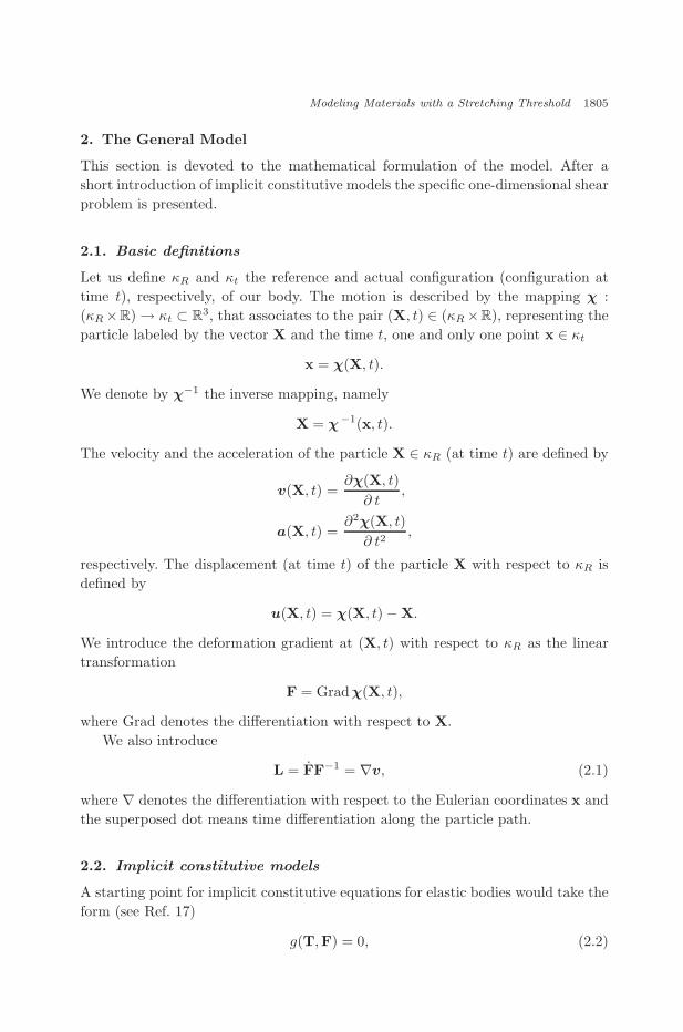
Modeling Materials with a Stretching Threshold 1837
we obtain
mα (t − t0) (1 − α)2 = mα (t − t0)(α + 1 − α2
) ⇒ α =32. (4.10)
So, for any m, the free boundary S (as long as it remains inside the domain D−S ) is
s(t) = 1 − 32
(t − t0)
and [[σ]]S grows linearly in time
[[σ]]S = mα2 (t − t0) (α − 1) ⇒ [[σ]]S =98m (t − t0) . (4.11)
Of course, the solutions can be continued but it becomes more involved.Let us now evaluate explicitly the total energy dissipated by the system. Using
first (2.36) for evaluating σ(s+, t), we get
τ0 − σ(s+, t) = −38m (t − t0) ,
and, from (2.59) and (4.11), we obtain the following expression for Pdiss (normalizedto τ2
0 /ρc)
Pdiss =(
38
)2 (t
t0− 1
)2
,
which fulfills inequality (2.60).
Case 2. σ is given by (4.6).
Applying the same technique which was employed to get (4.10) from (4.9), weobtain
mα (t − t0) (1 − α)2 = m (t − t0)[α(α + 1 − α2
)− 1], ⇒ (2α + 1) (α − 1)2 = 0,
whose solutions are α = 1 and α = −1/2 (the latter physically meaningless). Insuch a case S coincides with the characteristic Σ1+t0 , and (4.11) gives [[σ]]S = 0implying Pdiss = 0.
Case 3. σ is given by (4.7).
In such a case, t0 = 0 and f(y, t) ≡ 0 in the whole domain 0 < y < s(t), 0 < t < 1.We thus have a(s)(t) = − τ0
µ s and (2.49)4, (2.49)7, and (2.49)8 become− (1 − s) τ0 s = σ − s2τ0,
s(0) = 1,
s2(0) =σ
τ0.
(4.12)

November 5, 2007 20:35 WSPC/103-M3AS 00248
1838 A. Farina et al.
In particular, setting σ = γ2τ0, with γ2 > 1, and introducing the new dependentvariable r = 1 − s, (4.12) can be rewritten as
d
dt
(rdr
dt
)= γ2,
r(0) = 0,
r2(0) = γ2 ,
namely
r(t)r(t) − r (0) r(0)︸ ︷︷ ︸= 0
= γ2t , ⇒ d
dt(r2) = 2γ2t.
We thus have
r2(t) = γ2t2, ⇒ r(t) = γt ,
yielding s(t) = 1 − γt = 1 −√
bστ0
t, which is once again supersonic.
Concerning the dissipation (always normalized to τ20 /ρc), from (2.55) we have
Pdiss =γ
(γ2 − 1
)2
,
which corresponds to the half of the power supplied to the system.
Remark 4.2. For γ → 1 (i.e., σ → τ0) Pdiss tends to zero, in agreement withσ(s+, t) → τ0. Notice that, in this case, [[σ]]S does not vanish.
5. Comparison with a Piecewise Linear Hyperelastic Model
In this Sec. we shall see that the dynamics described in Sec. 4, case 1, cannot beretrieved as a limit case from the piecewise linear constitutive shown in Fig. 11 whenthe slope beyond the threshold tends to infinity, but as explained in the introductionthis is not surprising as the model with the moving interface is dissipative.
Let us consider the following stress–strain relation,l depending on theparameter λ
σ =
µε, 0 ≤ ε ≤ τ0
µ,
µλ2
(ε − τ0
µ
)+ τ0, ε >
τ0
µ,
with λ2 > 1, (5.1)
where ε = fy. The inverse of (5.1) is
ε =
σ
µ, 0 ≤ σ ≤ τ0,
σ − τ0
µλ2+
τ0
µ, σ > τ0.
(5.2)
lIn practice we are considering an elastic material characterized by two elastic moduli: µ if σ < τ0and µλ2 if σ > τ0.

November 5, 2007 20:35 WSPC/103-M3AS 00248
Modeling Materials with a Stretching Threshold 1839
Fig. 11. The “piecewise” linear constitutive relation.
Model (5.1) is hyperelastic, since the stress can be derived by the followingelastic energy
ψ (ε) =
µ
2ε2, 0 ≤ ε ≤ ε0,
µλ2
2(ε − ε0)
2 +µ
2(2ε ε0 − ε20
), ε > ε0,
with ε0 =τ0
µ, (5.3)
which, in terms of σ, can be rewritten as
ψ (σ) =
σ2
2µ, 0 ≤ σ ≤ τ0,
(σ − τ0)2µλ2
2
+τ0
µλ2(σ − τ0) +
τ20
2µ, σ > τ0.
(5.4)
Considering the problem treated in Sec. 4, case 1, for t ≥ t0 (i.e., after the time atwhich the applied load σ reaches the threshold τ0) the domain 0 < y < 1, t > t0has to be divided into two sub-domains, say D1 and D2, separated by a curvey = s(t), still denoted by S, such that:
• In D1 = 0 < y < s(t), t > t0 the governing equationm (written in dimensionlessform) is ftt − fyy = 0.
• In D2 = s(t) < y < 1, t > t0 the governing equation is ftt − λ2fyy = 0.
As opposed to the previous model we now have one more piece of additional infor-mation due to the presence of the elastic potential ψ, namely the energy in the
mRecall that ε = fy .

November 5, 2007 20:35 WSPC/103-M3AS 00248
1840 A. Farina et al.
system. Thus in addition to the conditions already known
kinematic : f(s−, t) = f(s+, t
), ⇒ [[v]]S = −s[[ fy]]S , (5.5)
dynamic : s[[v]]S = − 1µ
[[σ]]S , (5.6)
we may also write the energy conservation across S
s
(12[[v2]]S +
1µ
[[ψ]]S
)= − 1
µ[[σ v]]S . (5.7)
Proposition 5.1. Energy conservation implies that stress is continuous
σ(s+, t) = σ(s−, t) = τ0 ⇔ [[σ]]S ≡ 0. (5.8)
Proof. Using (5.5) and (5.6), we get from (5.7)
12[[σ]]S [[fy]]S + [[ψ]]S = σ(s+, t)[[fy]]S ,
or equivalently
[[ψ]]S =(
σ(s+, t) + σ(s−, t)2
)[[fy]]S . (5.9)
From (5.2) and (5.4)
[[fy]]S =σ(s+, t) − τ0
µλ2+
τ0 − σ(s−, t)µ
, (5.10)
[[ψ]]S =σ2(s+, t) − τ2
0
2µλ2− σ2(s−, t) − τ2
0
2µ. (5.11)
Substituting (5.10) and (5.11) into (5.9) we get
(τ0 − σ(s−, t))(σ(s+, t) − τ0)(1 − λ2) = 0. (5.12)
Thus either σ(s−, t) = τ0 or σ(s+, t) = τ0. From (5.5) and (5.6)
s2µ[[fy]]S = [[σ]]S ,
that is
s2(σ(s+, t) − τ0) + λ2s2(τ0 − σ(s−, t)) = λ2(σ(s+, t) − σ(s−, t)). (5.13)
If σ(s+, t) = τ0, then, from (5.13),
s2(τ0 − σ(s−, t)) = (τ0 − σ(s−, t)),
implying σ(s−, t) = τ0 or s2 = 1 (the latter meaning that s(t) = 1 − (t − t0), i.e.,the characteristic with slope −1). It is easy to check that s2 = 1 ⇔ σ(s−, t) = τ0.On the other hand, if σ(s−, t) = τ0 (and consequently s2 = 1), then, from (5.13)
(σ(s+, t) − τ0) = λ2(σ(s+, t) − τ0),

November 5, 2007 20:35 WSPC/103-M3AS 00248
Modeling Materials with a Stretching Threshold 1841
which yields σ(s+, t) = τ0, since λ2 > 1. Thus we conclude that in the bi-elasticmodel s(t) = 1 − (t − t0) and (5.8) follows.
Now, considering σ given by (4.5) (i.e. case 1 of Sec. 4), we have:
Domain D1. The displacement f is given by (4.8).
Domain D2. The displacement f is given by
f(y, t) = f(s−, t) +∫ y
s(t)
w (ξ, t) dξ =mt202µ
+∫ y
s(t)
w (ξ, t) dξ ,
with w solution of the Goursat problem
wtt − λ2wyy = 0, 1 − (t − t0) < y < 1, t0 < t,
w (Σ1+t0) =τ0
µ, t0 < t,
w (1, t) =1
µλ2(m t − τ0) +
τ0
µ, t0 < t,
(5.14)
i.e.
w(y, t) =τ0
µ− m
µλ2(1 − y − t + t0) ,
(recall τ0 = mt0). The analytical treatment of problem (5.14) for more general datais reported in Appendix A.
Let us now consider the limit λ → +∞, which should correspond, from thephysical point of view, to a material which cannot be strained as σ tends to τ0 (orε tends to ε0).
We first notice that (5.2) tends to the inverse of the graph reported in Fig. 4.In the limit λ → +∞ we have:
• S coincides with Σ1+t0 , so that σ(s−, t) = τ0.• In D1, f is still given by (4.8).• In D2, w(y, t) → τ0
µ and σ(y, t) = τ0 − m(1 − y − t + t0), i.e. the stress solvesσyy = 0,
σ(s+, t) = τ0,
σ (1, t) = mt .
However, in such a limit the dynamics breaks down. Indeed, [[σ]]S = 0 entails, byvirtue of (5.6), [[v]]S = 0, i.e. v(s) = mt0
µ = τ0µ . On the other hand, v(s)(t) may be
computed solving the equation of motion, that is
a(s) =σy
µ, ⇒ v(s)(t) = v(s) (0) +
m
µ(t − t0) ,
which contradicts v(s) = τ0µ .

November 5, 2007 20:35 WSPC/103-M3AS 00248
1842 A. Farina et al.
The reason why the model (5.2) fails to capture the response of our originalmodel with a threshold strain in the limit λ → +∞ lies essentially in the factthat the limit tends to preserve its hyperelastic character. Actually, recalling thenotation introduced in Sec. 2.5, it is easy to check that Eq. (5.7) entails Pdiss = 0 forany λ (consistent with the assumption of energy conservation). Indeed, normalizingthe total kinetic energy to ρc2h, its variation rate is (recall that in this case v isnot uniform for s < y < 1)
dK
dt= −1
2[[v2]]S s +
∫ s
0
vvtdy︸ ︷︷ ︸1µ
Rs0 (vσ)y−vyσ
+∫ 1
s
vvtdy︸ ︷︷ ︸1µ
R 1s
(vσ)y−vyσ
= −12[[v2]]S s − 1
µ[[σ v]]S +
1µ
v (h, t) σ︸ ︷︷ ︸Pext
− 1µ
∫ 1
0
vyσ dy,
while, for what concerns the variation rate of the total stored elastic energy (nor-malized to µh) we get
dΨdt
= − s
µ[[ψ]]S +
1µ
∫ s
0
ψtdy +1µ
∫ 1
s
ψtdy
= − s
µ[[ψ]]S +
1µ
s∫0
fy fy t dy
︸ ︷︷ ︸1µ
R s0 vyσ dy
+∫ 1
s
(λ2 (ε − ε0) + ε0
)︸ ︷︷ ︸σµ
fy t︸︷︷︸vy
dy
= − s
µ[[ψ]]S +
1µ
∫ 1
0
vyσ dy,
where (5.3) and (5.2) have been exploited. Thus, recalling (2.54), we have
Pdiss = Pext − d
dt(K + Ψ) =
12[[v2]]S s +
1µ
[[σ v]]S +s
µ[[ψ]]S = 0, because of (5.7).
In other words, model (5.2) is characterized by the absence of dissipation for any λ.The original problem, therefore, cannot be retrieved from a “piecewise” linearmodel.
Remark 5.1. The result just obtained can be extended to a more general non-linear stress–strain relationship σ = ϕλ(ε) = dψλ(ε)
dε , such that ϕλ, as λ → ∞,tends to the graph reported in Fig. 4. Indeed, by virtue of condition (5.7), anyhyperelastic model is characterized by Pdiss = 0.
If we want to construct a sequence which in the limit gives the same motion wehave studied in the previous sections, we must introduce some dissipation.
Remark 5.2. The same sequence of “bi-elastic” materials was considered in Refs. 7and 9 to approximate the original system by means of a penalization method.

November 5, 2007 20:35 WSPC/103-M3AS 00248
Modeling Materials with a Stretching Threshold 1843
Such a procedure, which clearly fails in our dynamical case for the reasons wehave explained, was successful in Refs. 7 and 9 in the context of equilibria, sincedissipation is obviously absent in that case.
6. The Uniaxial Extension Problem
Here we consider the motion of the form:x = X + f (X, t),
y = Y,
z = Z,
where (X, Y, Z) and (x, y, z) are typical points occupied by a material point in theundeformed and deformed configuration, respectively. Let h be the body length andlet us divide it into two regions:
• 0 ≤ X < s(t), corresponding to the elastic part.• s(t) ≤ X ≤ h, corresponding to the fully strained part.
In the elastic part the deformation gradient and the right Cauchy–Green tensor are
F =
fX + 1 0 0
0 1 0
0 0 1
, B =
(fX + 1)2 0 0
0 1 0
0 0 1
, (6.1)
and the stress is
T = µB.
Conservation of mass is expressed by
ρ(x, t) detF(X, t) = ρ0(X),
where ρ is density at time t > 0 and ρ0 is density at time t = 0. From (6.1) we have
ρ(x, t)[fX(X, t) + 1] = ρ0(X).
Conservation of linear momentum in the X coordinate direction yields
ρftt = µ∂
∂X
[(fX + 1)2
] ∂X
∂x,
that is
ρ0ftt = 2µ(fX + 1)fXX . (6.2)
If we make the assumption
|fX | 1 ⇒ x ≈ X,
that is we consider small deformations, then det(F) = 1 and ρ0 = ρ. With thisapproximation Eq. (6.2) becomes
ρftt = 2µfXX ,
which is equivalent to the shear problem considered before.
November 5, 2007 20:35 WSPC/103-M3AS 00248
1844 A. Farina et al.
However, in the traction problem the density may be discontinuous across theinterface introducing a substantial difference. The study of the traction problemwill be considered in a future paper.
7. Conclusions
We have formulated a mathematical model for the dynamics of materials possessinga strain threshold beyond which no deformation is allowed. More specifically wehave considered a motion of a layer of such a material which is kept fixed on oneboundary and subjected to a shear stress on the other, taking values beyond thethreshold.
This problem is suggested by the behavior of some biological tissues (e.g., ten-dons) which exhibit a sharply reduced deformability beyond some stretching thresh-old, and geological materials that exhibit the phenomenon of “locking.”
The mathematical structure of the problem is a hyperbolic free boundary prob-lem characterized by the fact that different initial and boundary data may producedifferent free boundary conditions. Accordingly, the stress (and the velocity field)may or may not exhibit a jump discontinuity on the free boundary itself. Themain physical difference between these two situations is that the discontinuous caseexhibits entropy production.
We have examined a class of problems in which the stress is continuous, empha-sizing that these situations correspond to somewhat artificial choices of the data,and we have proved a uniqueness and existence theorem for a sufficiently smalltime. In that case the interface is shown to be subsonic. Numerical computationshave been performed. We have also constructed a solution that for some time hasa stationary interface.
Problems with more natural sets of data (e.g., zero initial deformation and veloc-ity and constant or steadily increasing applied shear) have been studied, showingthat the interface is now supersonic and that the process is dissipative.
Finally we have considered a hyperelastic piecewise linear constitutive relation-ship and we have shown that the model with the strain threshold cannot be retrievedin this limit. The main physical reason being the fact that the piecewise linearhyperelastic model does not dissipate energy.
We believe that the present paper poses some interesting questions that shouldbe further investigated as the model under consideration is a good starting pointfor dealing with applications concerning biological and geological materials.
Appendix A. Problem (5.14) with Analytical Data
Let us consider problem (5.14), where in place of σ = mt we take a functionσ(t) ≥ τ0 which is analytic. We have the following:
Proposition A.1. Problem (5.14) has a unique solution, for σ(t) analyticfor t ≥ t0.

November 5, 2007 20:35 WSPC/103-M3AS 00248
Modeling Materials with a Stretching Threshold 1845
Proof. We first introduce the transformationz = 1 − y
θ = t − t0⇔
y = 1 − z
t = θ + t0
which implies that
∂
∂θ=
∂
∂t,
∂
∂z= − ∂
∂y,
∂2
∂z2=
∂2
∂y2,
and define the new dependent variable
u(z, θ) = −w (y (z, θ) , t (z, θ)) .
Problem (5.14) takes the form
uθθ − λ2uzz = 0, 0 < z < θ, 0 ≤ θ,
u (θ, θ) = −τ0
µ, 0 ≤ θ,
u (0, θ) = − 1µλ2
[σ(θ + t0) − τ0] − τ0
µ=: −η(θ), 0 ≤ θ,
(A.1)
whose characteristics are
θ ± z
λ= const.
Applying d’Alembert’s formula, we may write the solution of (A.1) as
u(z, θ) = −12
[η(θ − z
a
)+ η
(θ +
z
a
)]+
12
∫ θ+ za
θ− za
F (ξ)dξ,
where F (ξ) has to be determined imposing (5.14)2, i.e.,
−τ0
µ= −1
2[η (γθ) + η (βθ)] +
12
∫ βθ
γθ
F (ξ)dξ, (A.2)
where we set
γ = 1 − 1λ
and β = 1 +1λ
.
Differentiating (A.2) we get
η′(γθ)γ + η′(βθ)β − F (βθ)β + F (γθ)γ = 0. (A.3)
Since η is analytic (recall that σ is analytic for t ≥ t0)
η(ξ) =∞∑
k=0
ηkξk
and
η′(ξ) =∞∑
k=0
η′kξk, (A.4)

November 5, 2007 20:35 WSPC/103-M3AS 00248
1846 A. Farina et al.
where η′k = (k + 1)ηk+1, we look for a F (ξ) which is also analytic, that is
F (ξ) =∞∑
k=0
Fkξk. (A.5)
From (A.3)–(A.5)∞∑
k=0
θkFk(γk+1 − βk+1) + η′
k(βk+1 + γk+1)
= 0,
which provides the coefficients
Fk = η′k
[βk+1 + γk+1
βk+1 − γk+1
]= (k + 1) ηk+1
[βk+1 + γk+1
βk+1 − γk+1
].
Since γ < 1, β > 1 we have limk→∞ βk+1+γk+1
βk+1−γk+1 = 1, and
limk→∞
Fk+1
Fk= lim
k→∞k + 1
k
ηk+1
ηk= lim
k→∞ηk+1
ηk,
the series (A.5) has the same convergence radius as the power series of the func-tion η. So the existence is proved. Uniqueness in the class of bounded measurablefunctions follows by standard arguments.
Acknowledgment
This research was funded by the Italian MIUR Project “Problemi a FrontieraLibera.”
References
1. M. Aizenman and T. Bak, Convergence to equilibrium in a system of reacting poly-mers, Comm. Math. Phys. 65 (1979) 203–230.
2. C. Barus, Isothermals, isopiestics and isometrics relative to viscosity, Amer. J. Sci.95 (1893) 87–96.
3. B. Bernstein, Hypo-elasticity and elasticity, Arch. Rational Mech. Anal. 2 (1960)89–104.
4. B. Bernstein and K. R. Rajagopal, Thermodynamics of Hypoelasticity, accepted forpublication in ZAMP.
5. P. G. Ciarlet, Mathematical Elasticity, Vol. 1: Three Dimensional Elasticity (North-Holland, 1988).
6. J. Coirier, Mecanique des Milieux Continus (Dunod, 1997).7. J. E. Dunn and K. R. Rajagopal, Fluids of the differential type: Critical review and
thermodynamic analysis, Int. J. Eng. Sci. 33 (1995) 689–729.8. Y. C. Fung, Biomechanics: Mechanical Properties of Living Tissue (Springer-Verlag,
1993).9. L. Fusi and A. Farina, An extension of the Bingham model to the case of an elastic
core, Adv. Math. Sci. Appl. 13 (2003) 113–163.10. A. E. Green and P. M. Naghdi, Rate-type constitutive equations and elastic-plastic
materials, Int. J. Eng. Sci. 11 (1973) 725–734.

November 5, 2007 20:35 WSPC/103-M3AS 00248
Modeling Materials with a Stretching Threshold 1847
11. J. Hron, J. Malek and K. R. Rajagopal, Simple flows of fluids with pressure dependentviscosities, Proc. R. Soc. London A 457 (2001) 1603–1622.
12. J. D. Humphrey, Cardiovascular Solid Mechanics: Cells, Tissues and Organs(Springer-Verlag, 2002).
13. G. A. Johnson, G. A. Livesay, K. R. Rajagopal and S. Y. L. Woo, A single integralfinite strain (SIFS) viscoelastic model of ligaments and tendons, Adv. Bioeng. 22(1992) 245–248.
14. E. T. Olsen and B. Bernstein, A class of hypo-elastic non-elastic materials and theirthermodynamics, Arch. Rational Mech. Anal. 86 (1984) 291–303.
15. W. Prager, On ideal locking materials, Trans. Soc. Rheology 1 (1957) 169–175.16. W. Prager, Unilateral constraints in mechanics of continua, Estratto Dagli Atti Del
Simposio Lagrangiano (Accademia delle scienze di Torino, 1964), pp. 181–191.17. K. R. Rajagopal, On implicit constitutive theories, Appl. Math. 48 (2003) 279–319.18. K. R. Rajagopal, and A. R. Srinivasa, On the response of non-dissipative solids,
submitted for publication to the Proc. the Roy. Soc. Ser. A.19. K. R. Rajagopal, Elasticity of elasticity, to appear in ZAMP.20. K. R. Rajagopal, On implicit constitutive theories for fluids, J. Fluid Mech. 550
(2006) 243–249.21. R. S. Rivlin and J. L. Ericksen, Stress deformation relation for isotropic materials,
J. Rational Mech. Anal. 4 (1955) 323–425.22. I. Rubinstein and L. Rubinstein, Partial Differential Equations in Classical Mathe-
matical Physics (Cambridge University Press, 1998).23. H. U. Staubli, L. Schatzmann, P. Brunner, L. Rincon and L. P. Nolte, Mechanical
tensile properties of the quadriceps tendon and patellar ligament in young adults,Amer. J. Sports Med. 27 (1999) 27–34.
24. A. Z. Szert, Fluid Film Lubrication: Theory and Design (Cambridge University Press,1998).
25. C. Truesdell, Hypoelasticity, J. Rational Mech. Anal. 4 (1955) 83–133.26. C. Truesdell and W. Noll, The Nonlinear Field Theory of Mechanics, in Handbuch
der Physik, ed. Flugge, Vol. III/3 (Springer, 1965).27. C. Truesdell and H. Moon, Inequalities sufficient to ensure semi-inversibility of
isotropic functions, J. Elasticity 5 (1975) 183–189.28. V. S. Vladimirov, Equazioni della Fisica Matematica, Edizioni (MIR, 1987).29. L. Rubinstein, The Stefan Problem, Translations of Mathematical Monographs,
Vol. 27 (Amer. Math. Soc., 1971).30. R. N. Vaishnav and D. J. Patel, Basic Hemodynamics and Its Role in Disease Process
(MTP Press, 1980).