Materials Testing
468
Application Handbook Materials Testing
-
Upload
khangminh22 -
Category
Documents
-
view
0 -
download
0
Transcript of Materials Testing

Application Handbook
Materials Testing

Introduction
Consumer and environmental protection, healthcare, quality control and product safety are key issues being pursued rigor-ously. In order to meet the requirements of international mar-kets, standards and norms such as ISO, testing and inspection machines are applied in a vast number of industries. They help to support human health and individual well-being while pre-venting accidents and damage, enhancing comfort levels and enjoyment and providing peace of mind. Furthermore, testing machines offer data which serves to guide R&D towards improved materials and products.
This Materials Testing Application Handbook covers 112 appli-cations of 8 industries, such as automotive, aerospace, bioma-terials and medical, composites, food, metal, railroad, rubber and plastics industries. It is hands-on and solution-oriented. The applications described cover most-modern technologies, e.g. universal, fatigue and hardness testing and also high-speed video camera application.
Since 1917, Shimadzu has been manufacturing testing machines designed to meet the diverse needs of customers worldwide. To date, Shimadzu has sold tens of thousands of testing machines based on our primary product lines, includ-ing the Autograph series precision universal testers, UH series universal testing machines and Servopulser series fatigue test-ing machines. In addition, Shimadzu has marketed thousands of application-specific systems tailored to the unique needs of clients, and remains committed to providing customers with this same level of service in the future.
In addition to testing machines and equipment, Shimadzu as a worldwide leading manufacturer of analytical instrumentation systems provides high-level, sophisticated solutions in liquid and gas chromatography, mass spectrometry, TOC analysis, spectroscopy, consumables and software.
Our brand statement “Excellence in Science”, reflects our desire and intention to respond to customer requirements by offering superior, world-class technologies. With a worldwide network of subsidiaries in 76 countries and circa 10.000 employees Shimadzu guarantees personal support for each customer.
Please see also our Application Handbooks on • Liquid Chromatography• Food & Beverages• TOC• Clinical• GC/GC-MS.
www.shimadzu.eu/materials-testing-inspection

Contents
1. Automotive Industry
2. Aerospace Industry 3. Biomaterials and Medical Industry 4. Composite Industry 5. Food Industry 6. Metal Industry 7. Railroad Industry 8. Plastics and Rubber Industry 9. Others

1. Automotive Industry

1. Automotive Industry
EMOTION, SAFETY, COMFORT AND FUN
Cars are much more than just a means of transportation: although automobiles are technical products, they carry emotion, provide safety, offer comfort and generate fun. Cars are also part of cultures, and they play a role in business, private and family lives. Depending on the behavior of each single driver, cars can also be a means to endangering other road users.
The many tiers of the automotive industries provide a great deal of applications for material testing and inspection machines to make cars safer, more comfortable, efficient and environmentally responsible. The testing machines are used for engines, motors and power sources; bodies and interiors;
lithium-ion rechargeable batteries and fuel cells; suspension and other power transmission systems; electronic instrumenta-tion components and environmental conservation.
Cars may be the most complex technical mass market prod-ucts which are comprehensively tested on a worldwide scale. International testing standards apply to single components as well as to cars as a whole. Please see the applications on the following pages for an overview of the wide range of test-ing. Materials tested are metals, non-metals and composites tested with destructive (Destructive Physical Analysis DPA) or non-destructive testing (NDT) methods in order to evaluate the properties of a material, component or system.

1. Automotive Industry
C225-E033 Three-axis endurance evaluations of automobile steering mechanisms
No.i245 Evaluation of temperature-dependent strength properties of lithium-ion battery separator by piercing and tensile testing
SCA_300_002 MCT compression test for structural materials of lithium-ion batteries
SCA_300_011 Evaluation of adhesive strength and hard- ness of protective surface layer of glass substrates
SCA_300_012 Evaluation of hardness of painted surface with Shimadzu dynamic ultra micro hard- ness tester model DUH
SCA_300_019 Hardness evaluation of thin film with Shimadzu dynamic ultra micro hardness tester
SCA_300_040 Evaluation of hardness of painted surface
SCA_300_049 Seat belt test tensile test according to manufacturer’s specification
eV022 High-speed imaging of fuel injection in automotive engines
No.ei254 Compression after impact testing of composite
No.ei255 Compression testing of composite materials
No.36 Evaluating the fatigue strength of GFRP materials
No.30 Evaluating the strength of carbon fiber reinforced plastics (CFRP)
No.39 Evaluation of open-hole CFRP
No.i247 DIC analysis material testing by strain distribution visualization
No.8 Flexural testing of CFRP boards
No.16 Tensile testing of carbon fiber
No.31 Materials testing using digital image correlation
No.37 Observing the failure of open-hole CFRP samples in tensile tests
No.38 Observing the fracture of unidirectional CFRP in static tensile testing
No.ei256A Open-hole compression testing of composite material
No.ei250 Shear test of composite material (V-notched beam)
No.ei251 Shear test of composite material (V-notched rail shear)
SCA_300_037 Compression-rupture test of carbon fibers with different tensile characteristics Shimadzu micro compression testing machine MCT
SCA_300_059 Observation of fracture in CFRP tensile test E001HPV
C225-E032 Ultrasonic fatigue testing system with an average stress loading mechanism
No.i244 Tensile test for metallic materials using strain rate control and stress rate control
SCA_300_035 A hardness measurement of surface treat- ment layer on a steel sample using Shimadzu dynamic ultra micro hardness tester, model DUH
SCA_300_045 Jigs for measuring Bauschinger effect
No.2 Flexural test of plastic ISO178
No.3 Tensile tests of plastic materials at low ISO527 1
No.4 Tensile test of rubber dumb bell specimens ISO37
No.5 Tear test of crescent shaped ISO34 1
No.6 Tear tests of angle shaped rubber specimens ISO34 1
No.7 Tensile tests of films ISO527 3
No.9 Measurements of modulus of elasticity and poisson’s ratio for films ISO527
Steering mechanism unit
System Appearance
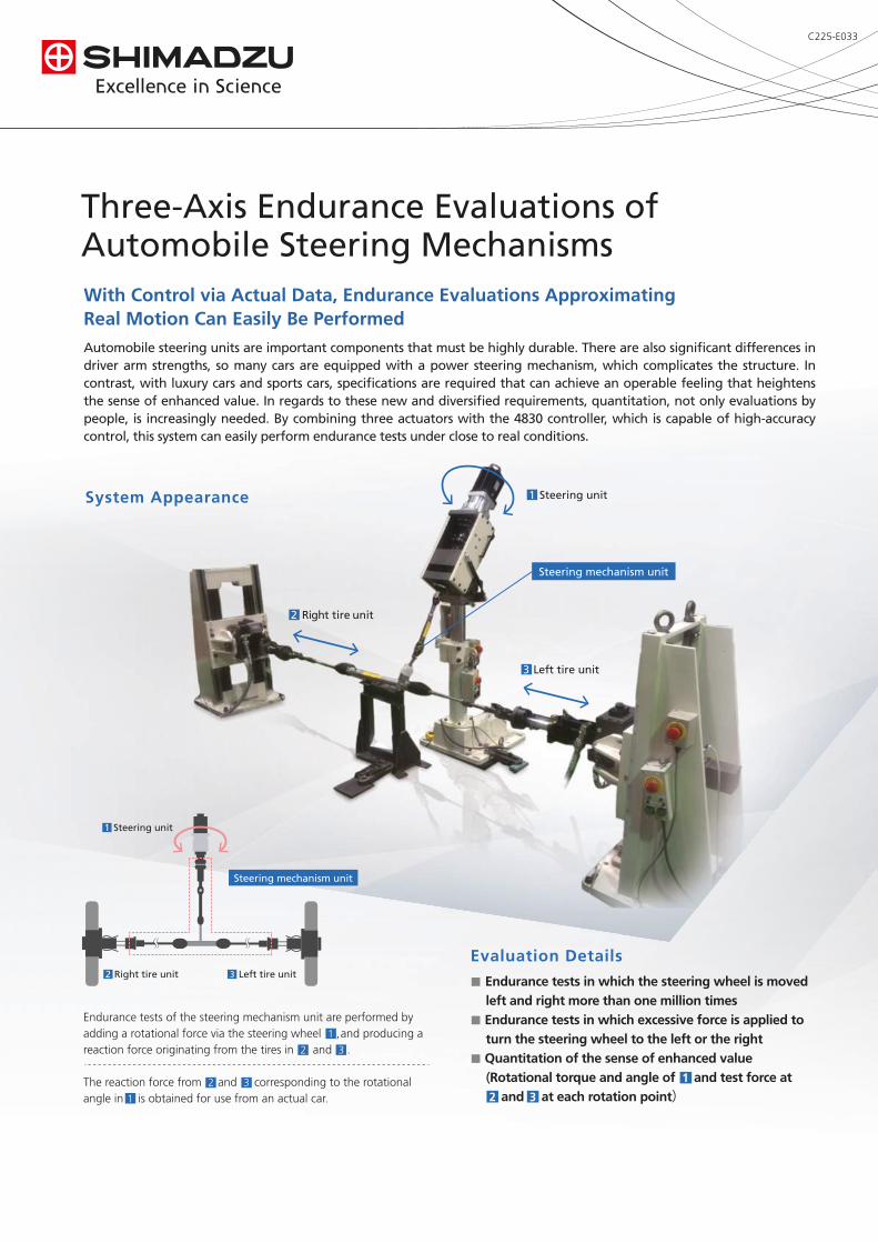
Automobile steering units are important components that must be highly durable. There are also significant differences in driver arm strengths, so many cars are equipped with a power steering mechanism, which complicates the structure. In contrast, with luxury cars and sports cars, specifications are required that can achieve an operable feeling that heightens the sense of enhanced value. In regards to these new and diversified requirements, quantitation, not only evaluations by people, is increasingly needed. By combining three actuators with the 4830 controller, which is capable of high-accuracy control, this system can easily perform endurance tests under close to real conditions.
1 Steering unit
3 Left tire unit
2 Right tire unit
Evaluation Details
■ Endurance tests in which the steering wheel is moved left and right more than one million times■ Endurance tests in which excessive force is applied to turn the steering wheel to the left or the right■ Quantitation of the sense of enhanced value (Rotational torque and angle of 1 and test force at 2 and 3 at each rotation point)
Steering mechanism unit
Three-Axis Endurance Evaluations ofAutomobile Steering MechanismsWith Control via Actual Data, Endurance Evaluations ApproximatingReal Motion Can Easily Be Performed
3 Left tire unit2 Right tire unit
1 Steering unit
Endurance tests of the steering mechanism unit are performed by adding a rotational force via the steering wheel 1 , and producing a reaction force originating from the tires in 2 and 3 .
The reaction force from 2 and 3 corresponding to the rotational angle in 1 is obtained for use from an actual car.
C225-E033

4830 Controller
Main Specifications
Left/Right Tire Units 1) Rated capacity: ±10 kN stroke ±100 mm
(static maximum load capacity ±13 kN)
2) With trunnion pin
3) Maximum speed: 500 mm/sec
(20 L/min hydraulic source, when unloaded)
Lifting Stand(For the left/right tire units)
1) Height: 300 mm to 800 mm
(electric lift, manual bolt fastening)
2) Angle: top/bottom ±10°
(can change fastened or mobile) and horizontal ±10°
Steering Unit 1) Rated capacity: ±200 Nm, Angle: ±1080 deg
2) Maximum speed: 360 deg/sec
3) Excitation frequency: 0.01 Hz to 2 Hz (±5 deg or more)
Lifting Stand(For the steering unit)
1) Height: 800 mm to 1200 mm (electric lift, manual bolt fastening)
2) Angle: top/bottom 0° to 60° (can change fastened or mobile)
Data Processing Example (PC Screen) The left window shows the data chart results when
the steering unit is turned to the left and right from
the center position, and then returns to the center.
The window on the left shows a chart of angle versus test force.
The window on the right shows a chart of time versus test force.
The blue line is the test force for the right tire unit.
The red line is the test force for the left tire unit.
© Shimadzu Corporation, 2016First Edition: August 2016

ApplicationNews
No.
LAAN-A-AG-E010
Material Testing System
Evaluation of Temperature-Dependent Strength Properties of Lithium-Ion Battery Separator by Piercing and Tensile Testingi245
Lithium-ion secondary cells, also called rechargeable batteries, (referred to here as "lithium-ion batteries") are widely used as energy sources for information terminals and consumer electronics, etc. because of their high energy density and cell voltage. Recently, their growing rate of dissemination into areas of general household applications, including hybrid and electric vehicles, is quite evident, and it appears obvious that the demand will further increase in the future. Because lithium-ion batteries can sometimes become unstable due to short-circuit, over charging and discharging, impact, etc., a variety of protection mechanisms are incorporated at the battery component level to ensure safety.Of these component parts, the lithium-ion battery separator prevents contact between the positive and negative electrodes, while at the same time playing a role as a spacer which permits the passage of lithium ions. However, it also performs the function of
preventing a rise in battery temperature due to excessive current in the event of a short circuit. Because the lithium-ion battery separator is set in place so that it comes into contact with the rough surfaces of the positive and negative terminals, high mechanical strength is required. This mechanical strength must be maintained even if there is some rise in temperature, which is common to some degree, for example, during battery charging. Therefore, we conducted piercing and tensile testing measurements of the separator to evaluate changes in strength with respect to changes in temperature. This document introduces actual examples of these tests.
Supplement) Regarding the lithium-ion battery separator, previous evaluation examples were also introduced in Application News T146 "Measurement of Separator in Lithium-Ion Battery" and i229 "Multi-Faceted Approach for Evaluating Lithium-Ion Battery Separators."
The samples consisted of separators removed from two lithium-ion batteries (cylindrical) used in small electrical devices, and we measured the changes in piercing characteristics due to changes in environmental
temperature. Fig. 1 shows an overview of the test conditions, and Table 1 presents details of the test conditions.
n Introduction
n Piercing Test
Fig. 1 Overview of Piercing Test

Table 1 Test Conditions (Piercing Test)
Table 2 Summary of Results (Piercing Test)
1) Instrument Shimadzu AG-X Precision Universal Tester
2) Load cell capacity 1 kN
3) Jigs Boil-in-bag piercing jig
4) Thermostatic chamber TCR-1W
5) Load rate 50 mm/min
6) Temperature 25 °C, 60 °C, 90 °C
7) Software TRAPEZIUMX (Single)
Temperature (°C) Maximum Force (N) Maximum Displacement (mm)
25 3.85 4.45
60 4.07 6.63
90 2.13 6.68
Fig. 2 shows the force – displacement curve, and Table 2 shows the maximum force and maximum displacement with respect to temperature.Comparing the test results at 25 °C and 60 °C, it is evident that there is not much difference in the maximum force, but the maximum displacement is greater at 60 °C. Comparing characteristic values at 60 °C and 90 °C, the decrease in maximum force is obvious at 90 °C, but the maximum displacement value is about the same. From the above, it can be assumed that at 60 °C, there is no decrease in strength of the lithium-ion battery separator, despite the apparent increase in its elongation property.
The separators used for the tensile testing were removed from commercially available lithium-ion batteries (square-shaped), so 2 types of samples (below, referred to as samples (1) and (2)) which contained PE (polyethylene) as the principle constituent were used. When conducting the tensile tests, each separator
sample (as shown in Fig. 3(a)) was fashioned into dumbbell-shaped specimens oriented in the lengthwise and widthwise directions of each separator, as shown in Fig. 3(b). The total length of all specimen was 35 mm, with the parallel section measuring 10 (L) × 2 (W) mm.
n Tensile Test
Fig. 2 Test Result (Piercing Test)
Fig. 3 Test Samples
Displacement (mm)
5.0
4.5
4.0
3.5
3.0
2.5
2.0
1.5
1.0
0.5
0.00 1 2
25 °C 60 °C
90 °C
3 4 5 6 7 8 9 10Fo
rce
(N)
Widthwise direction
Leng
thw
ise
dire
ctio
n
(a) Separator Sample (b) Dumbbell-Shaped Specimens (image)
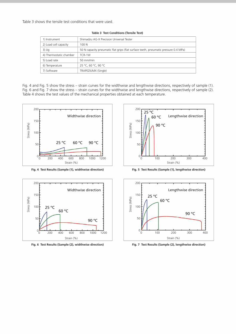
Fig. 4 and Fig. 5 show the stress – strain curves for the widthwise and lengthwise directions, respectively of sample (1). Fig. 6 and Fig. 7 show the stress – strain curves for the widthwise and lengthwise directions, respectively of sample (2). Table 4 shows the test values of the mechanical properties obtained at each temperature.
Table 3 shows the tensile test conditions that were used.
Fig. 4 Test Results (Sample (1), widthwise direction)
Strain (%)
200
150
100
50
00 200 400 600 800 1000 1200
Widthwise direction
25 ºC 60 ºC 90 ºC
Stre
ss (M
Pa)
Fig. 5 Test Results (Sample (1), lengthwise direction)
200
150
100
50
00 100 200 300 400
Strain (%)
Lengthwise direction25 ºC
60 ºC
90 ºCSt
ress
(MPa
)
Fig. 6 Test Results (Sample (2), widthwise direction)
200
150
100
50
00 200 400 600 800 1000 1200
Strain (%)
Widthwise direction
25 ºC60 ºC
90 ºC
Stre
ss (M
Pa)
Fig. 7 Test Results (Sample (2), lengthwise direction)
200
150
100
50
00 100 200 300 400
Strain (%)
Lengthwise direction
25 ºC60 ºC
90 ºC
Stre
ss (M
Pa)
Table 3 Test Conditions (Tensile Test)
1) Instrument Shimadzu AG-X Precision Universal Tester
2) Load cell capacity 100 N
3) Jig 50 N capacity pneumatic flat grips (flat surface teeth, pneumatic pressure 0.4 MPa)
4) Thermostatic chamber TCR-1W
5) Load rate 50 mm/min
6) Temperature 25 °C, 60 °C, 90 °C
7) Software TRAPEZIUMX (Single)

For Research Use Only. Not for use in diagnostic procedures.The contents of this publication are provided to you “as is” without warranty of any kind, and are subject to change without notice. Shimadzu does not assume any responsibility or liability for any damage, whether direct or indirect, relating to the use of this publication.
First Edition: January, 2012
www.shimadzu.com/an/ © Shimadzu Corporation, 2012
In each of the samples, a lower tensile strength and greater elongation was seen in the widthwise direction than in the lengthwise direction. When comparing the numbers in Table 4, the lengthwise tensile strength for sample (1) is about 5 times greater than the widthwise tensile strength of sample (1). Also, the strain at break, for sample (1) in the lengthwise direction is lower by about a factor of 15 than that of sample (1) in the widthwise direction. From the above results, it is supposed that this separator (sample (1) ) was manufactured using uniaxial drawing in the lengthwise direction. The widthwise tensile strength for sample (2) is about twice that of sample (1), and the strain at break is much lower. The tendency similar to that of sample (2) in the widthwise direction is seen with respect to sample (2) in the lengthwise direction. Therefore, due to the tendency of greater tensile strength and lower strain at break with sample (2) in the lengthwise direction, it is presumed that sample (2) was manufactured with a low biaxial drawing ratio, and that the drawing ratio in the lengthwise direction was greater than that in the widthwise direction. The data obtained regarding the mechanical properties with respect to the sample temperature are also
interesting. When comparing the sample strain at break and tensile strength at 25 °C and 60 °C, even though the strain at break value increased by a factor of 2 due to the test temperature increase to 60 °C, there was just a slight decrease in tensile strength. Similarly, when comparing the physical property measurement values at 60 °C and 90 °C, the strain at break showed the same tendency to greatly increase as when the values were compared at 25 °C and 60 °C. However, in this case, the tensile strength value shows a significant decrease. From the above, it is evident that the lithium-ion battery separators used in this test maintain excel lent mechanical strength at 60 °C, notwithstanding its elevated elongation characteristics. High-mechanical strength specifications are required for separators in order to withstand changing temperature in the cell. Here, as is clear from the results of piercing and tensile testing of lithium-ion battery separators under atmospheric temperature control, the mechanical properties of lithium-ion battery separators can be reliably evaluated using the Shimadzu Precision Universal Tester AG-X with its abundant array of accessories.
Table 4 Summary of Results of Tensile Test
25 °C 60 °C 90 °C
SampleTensile Strength
(MPa)Strain at Break
(%)Tensile Strength
(MPa)Strain at Break
(%)Tensile Strength
(MPa)Strain at Break
(%)
(1) Widthwise direction 36.9 471.4 35.4 898.8 19.3 1044.0
(1) Lengthwise direction 175.6 26.8 162.5 57.0 129.9 76.7
(2) Widthwise direction 78.2 138.5 68.8 347.6 33.8 427.9
(2) Lengthwise direction 129.5 34.1 118.3 105.3 58.7 367.2

■Introduction Since lithium-ion batteries are light and small, they are used in a wide variety of products, from mobile electronic devices such as cellular phones and notebook PCs to electric cars and hybrid cars. Their inner structural materials are subjected to external force during production processes and to pressure during use. Therefore, evaluation of strength of each structural material is important to maintain consistent quality. A strength measurement was performed on thin or minute materials among various structural materials of lithium-ion batteries. Separators are
usually evaluated by a tensile test or penetration test. A compression test is also important to evaluate them because they are compressed in some processes. Active materials of approximately 10 μm in size located near the electrode need to have a certain compression strength so they will not be destroyed during the coating process. Below are the results of compression tests performed on these materials using the MCT-211 Series Micro Compression Testing Machine.
Fig. 1 External View of the MCT-211 Series (with the Side Observation Kit Mounted)
Fig. 2 Structure of Lithium-Ion Battery
Material Testing System MCT
Compression Test for Structural Materials of Lithium-Ion Batteries by MCT
No. SCA_300_002

■Compression Test on Separator of Lithium-Ion Battery
Table 1 shows the three types of specimens used for the measurement. Table 2 shows accessories used in the test and test conditions. Fig. 3 shows the conceptual diagram of the measurement. Table 3 shows the results of the compression tests on the three types of specimens. The specimens were evaluated by a compression rate where the same test
force was applied. The results clearly show the difference among the three types. Fig. 4 is a graph indicating the test force - displacement relationship of each specimen. The inflexion point of specimen 2 is at around 10 mN (pressure of approximately 5 MPa), indicating that applying too much compression pressure causes plastic deformation to the separator.
Table 1 Specimens 1) Specimen Name Separator
2) Specimen Number 1 2 3
3) Thickness 20 μm 20 μm 10 μm
Table 2 Test Conditions 1) Upper Indenter Flat indenter (with a
diamond tip), 50 μm dia.
2) Test Mode Load-unload test 3) Test Force (mN) 50
4) Loading Rate (mN/sec)
2.2
5) Holding Time (sec) 0
6) Test Method A thin layer of liquid glue was applied to a glass plate, the separator was bonded to it, and a compression test was performed using the upper indenter. (See Fig. 2.)
Fig. 3 Conceptual Diagram of Measurement
Table 3 Test Results Specimen Name Specimen Number Maximum Force (mN) Compression Variation (μm) Compression Rate (%)
Separator 1 49.9 3.651 18.3 2 49.9 3.371 16.9 3 50.0 1.038 10.4
Note: The compression rate was calculated by the following calculation formula. Compression rate (%) = (compression volume)/(thickness) × 100 (%)
No.SCA_300_002

Fig. 4 Results of Compression Test
■Compression Test on Active Materials A compression test was performed on two types of active material particles for positive electrode of lithium-ion battery. Table 4 shows test conditions and Fig. 5 shows an image of the test (compressed part). Measurement was performed ten times for each specimen. Then, average values were selected as a representative value for each specimen. (See Table 5 and Fig. 6.) The results clearly indicate the difference
in the strength between the two active materials and lithium cobalt oxide (LiCoO2) was confirmed to have the higher strength. As shown above, the MCT-211 Series Micro Compression Testing Machine enables accurate and efficient evaluation of compression characteristics of thin or minute materials used inside lithium-ion battery.
Table 4 Test Conditions
1) Upper Indenter Flat indenter (with a diamond tip), 50 μm dia.
2) Test Mode Compression test 3) Test Force (mN) 50 4) Loading Rate
(mN/sec) 2.2
5) Holding Time (sec) 0 6) Test Method A very small amount of
each specimen was spread on the lower compression plate and a compression test was performed on each single particle. (See Fig. 5.)
Fig. 5 Conceptual Diagram of the Compressed Part
No.SCA_300_002

Table 5 Test Results Specimen Name Fracture Force (mN) Particle
Diameter (μm) Strength (MPa)
LiMn2O4 1.67 13.0 7.79 LiCoO2 16.23 13.3 72.75
Note: Fracture strength was calculated by the following calculation formula (Based on JIS R1639-5∗1). Cs = 2.48 P/πd2 Cs: Strength (MPa), P: Fracture force (N), d: Particle diameter (mm)
∗1: Test methods of properties of fi ne ceramic granules Part 5: Compressive strength of a single granule
Fig. 6 Force - Displacement Curves
No.SCA_300_002

Rapid progress of thin film developing technology has accelerated expansion of film applications. Thin film developing technologies based on vacuum evaporation, sputtering, or ion plating are featured not only in the improvement in quality of thin films, but also in adding new characteristics to a material, and are applied in various fields such as semiconductors, optical materials, and machine parts. Adhesive strength and hardness are important factors for the evaluation of the mechanical strength of thin film that is produced by the aforementioned techniques. Thin film that satisfies specifications of quality and properties may peel from its substrate board unless its adhesive strength is adequate. There may also be a problem of unimpeded wear and tear, if its hardness does not conform to specifications. The following is an introduction to an evaluation of adhesive strength and hardness of a thin film on a glass substrate with Shimadzu Scanning Scratch Tester Model SST and Shimadzu Dynamic Ultra Micro Hardness Tester Model DUH.
■ Test conditions
SST-101: (1) Stylus (needle): Diamond 100 µm (2) Swing amplitude: 60 µm (3) Scratch speed: 20 µm/s (4) Max load: 20 gf (5) Down speed of cartridge: 1 µm/s
DUH-211:
(1) Testing mode: Indenter pressing test (2) Load: 2 gf (3) Loading rate constant: 1 (0.029 gf/s) (4) Indenter: 115° triangular pyramid
■ Test piece
1) Name: Surface protective thin film of glass substrate
2) Type: 1 through 3 3) Thickness of films: approx. 1µm or all
Test piece
Peeling load (gf) 1 2 3 4
No. 1 1.3 1.4 1.3 1.33 No. 2 2.5 2.4 2.5 2.47 No. 3 7.4 7.4 7.1 7.30
Table 1: Test results of SST
Material Testing System DUH
Evaluation of Adhesive Strength and Hardness of Protective Surface Layer of Glass Substrates
No. SCA_300_011

No. SCA_300_011
■ Test results
Figure 1: Load – cartridge output curves of test piece No.1 (with SST)
Figure 2: Load – cartridge output curves of test piece No.2 (with SST)
Figure 3: Load – cartridge output curves of test piece No.3 (with SST)
Figure 4: Load – indentation depth curves of test piece No.1 (with DUH)
Figure 5: Load – indentation depth curves of test piece No.2 (with DUH)
Figure 6: Load – indentation depth curves of test piece No.3 (with DUH)

No. SCA_300_011
Figure 7: Hardness Distribution in Depth Direction
Hardness distribution was calculated by the following equation (Data analysis 2: Output data of load and indentation depth) as internal hardness distribution is not known from load-indentation depth curves.
𝐷𝐷𝐷𝐷𝐷𝐷𝐷𝐷𝑚𝑚𝑚𝑚−𝑛𝑛𝑛𝑛 =37,838 ∙ 𝑃𝑃𝑃𝑃𝑛𝑛𝑛𝑛 ∙ �1 −�𝑃𝑃𝑃𝑃𝑚𝑚𝑚𝑚𝑃𝑃𝑃𝑃𝑛𝑛𝑛𝑛
�2
(𝐷𝐷𝐷𝐷𝑛𝑛𝑛𝑛 − 𝐷𝐷𝐷𝐷𝑚𝑚𝑚𝑚)2 Where DHm-n: Hardness at indentation depth from Dm to Dn. Pm, Pn: Load (gf) Dm, Dn: Indentation depth (µm)
The result of peeling strength tests of surface protective films Nos.1-3 on glass substrates tested with Model SST-101 are shown in Table 1, from which it is known that adhesive strength estimated by the peeling load is greatest in the test piece No. 3 followed by No. 2 and No. 1, respectively. The hardness measurement's result is shown in Figs.4-6 in the form of load versus indentation depth curves. Hardness variation in depth direction is plotted in Fig.7 as well. According to this
graph, it is known that the thin film hardness in the ultra-surface of specimen No. 3 is greatest among the three, and also that hardness of all the specimens gets lower at a depth below 0.5 μm, probably because cracks (ruptures) were produced during indentation. According to the hardness distribution curves from the surface down to 0.5 μm, hardness of test piece No. 3 (high adhesive strength) increases gradually, while the hardness of No. 1 (less adhesive strength) stays virtually unchanged.

Painted surfaces are evaluated for properties such as weathering resistance, light resistance, adhesive strength, impact resistance and hardness by instrumental measurement, and for color, gloss, unevenness, rumples etc. by visual inspection. Of these, the hardness test of painted surfaces is most important in evaluating the quality of paint film. Wet paint is dried in order to transform wet paint into rigid paint film. Paint can be dried either by the natural drying method, in which the paint dries completely at room temperature, or by the forced drying method,
in which paint is dried under high temperatures of approx. 100 to 250 degrees Celsius. The surface hardness of paint films differs depending on the kind of paint and the drying method. Information for evaluating hardness near the surface of paint film can be obtained by the ultra micro area measuring technique of the Shimadzu Dynamic Ultra Micro Hardness Tester Model DUH. The following presents the results of hardness tests performed on paint films of paints for general use dried either by the natural or by the forced drying method.
Material Testing System DUH
Evaluation of Hardness of Painted Surface with Shimadzu Dynamic Ultra Micro Hardness Tester Model DUH
No. SCA_300_012

No. SCA_300_012
■ Measurement of surface hardness of paint films Testing machine
Table 1 Test Conditions
(1) Paint film of meramin resin dried by forced drying
Fig.1 Indentation depth Load Curves of
Painted Films of Meramin Resin
(2) Paint film of urethane resin dried by natural drying
Fig.2 Indentation Depth Load Curves of
Painted Films of Urethane Resin
(3) Paint film of acrylic resin dried by natural drying
Fig.3 Indentation Depth Load Curves of Paint
Films of Acrylic Resin
TEST MODE 2
CAL. MODE 1 ( 115° Triangular Pyramid Indenter )
AUTO or MANUAL AUTO F.S. DEPTH 2 & 5 µm MAX LOAD 9,81mN & 49,03 mN LOADING SPEED
1 (0,1,4632 [mN/sec]) 5 (13,3240 [mN/sec] )
TOUCH SPEED
50 ( 0,48 [mN/sec] ) 50 ( 0,048 [mN/sec] )
AFTER TIME 5 sec. PRE TIME 5 sec. LOT 5

No. SCA_300_012
■ Result of Measurements
Sample Name LOAD (mN) DH (mean) Meramin resin paint film thickness 38 µm -
forced drying 9,81 mN 14,60
Overall thickness of paint film 177 µm 49,03 mN 12,00 Urethane resin paint film thickness 48 µm -
forced drying 9,81 mN 13,00
Overall thickness of paint film 84 µm 49,03 mN 5,20 Acrylic resin paint film thickness 52 µm -
forced drying 9,81 mN 10,50
Overall thickness of paint film 110 µm 49,03 mN 4,90 Table 2 Result of Measurements
Dynamic hardness is obtained based on the load value and indentation depth during the loading process. Since dynamic hardness is calculated from the indentation depth during the loading process, it includes both plastic deformation and elastic deformation. DH: dynamic hardness F: test load mN h: dynamic indentation depth2
DH115 = 3.8584×F/h2 DHT115: Dynamic hardness obtained with the triangular pyramid indenter with 115°tip angle
When LOAD is small, DEPTH is small, allowing the hardness of paint film at the outermost surface to be measured. When LOAD is large, DEPTH is also large, allowing the hardness at the deeper portion of paint film to be measured. In tests on samples dried by natural drying and forced drying, a different trend was observed for the respective samples between the results of 9,81 mN and 49,03 mN LOADs. In other words, the difference between the data for 9,81 mN and 49,03 mN was large in case of natural drying, while significantly smaller in the case of forced drying. This indicates that forced drying creates hardness more evenly distributed throughout the depth of the paint film than natural drying. * Please be advised that data obtained before the implementation of the current Weights and Measures Law may be presented in terms of gravimetric unit.

■ Introduction Thin film production technology has made a rapid progress and a great quantity of thin films are put to practical use in various applications. The evaluation of the hardness of thin films produced by CVD and PVD and surface coating layers plays an important role in production technology. In spite of such background, this method has not yet been definitively standardized, though some technical reports on hardness evaluation based on micro hardness method have been issued. The Shimadzu Dynamic Micro Hardness Tester Model DUH, designed as a hardness evaluating machine, is also useful in the thin film market where a low electromagnetic load applying system is needed for information of material strength of a micro area on the basis of micro load measuring and controlling technique.
Fig. 1 External View of the DUH-211 series
In addition, a new method was developed for calculating dynamic hardness from the difference between two indentation depths at any two different loads, enabling calculation
of hardness distribution in the depth direction. The following presents the results of two recent measurements. ■ Relation of load and indentation depth of a-Si thin film produced by CVD DH hardness is calculated using the following equation, where D1 and D2 are depths at any two points on the chart and P1 and P2 are loads corresponding to D1 and D2 respectively.
𝐷𝐷𝐷𝐷𝐷𝐷𝐷𝐷 = 𝛼𝛼𝛼𝛼 =𝑃𝑃𝑃𝑃2
(𝐷𝐷𝐷𝐷2 − 𝐷𝐷𝐷𝐷1)2∙ �1 −�
𝑃𝑃𝑃𝑃1𝑃𝑃𝑃𝑃2�
2
The distances between D1 and D2 can be set freely. If D points are set at regular intervals, hardness distribution in depth direction is calculated.
Fig. 2 Relation of Load versus Dynamic
indentation depth of a-Si thin film
Material Testing System DUH
Hardness Evaluation of Thin Film with Shimadzu Dynamic Ultra Micro Hardness Tester (II) No. SCA_300_019

No. SCA_300_019
■ Evaluation of hardness distribution in depth direction for several kinds of thin films made by CVD Hardness variation in the depth direction is shown for each thin film. These curves are useful to determine how hardness varies according to thin film processing conditions. * Please be advised that data obtained before the implementation of the current Weights and Measures Law may be presented in terms of gravimetric unit
Fig. 3 Evaluation of Hardness distribution in depth direction for several kinds of thin films produced
by CVD

Painted surfaces are evaluated for properties such as weathering resistance, light resistance, adhesive strength, impact resistance and hardness by instrumental measurement, and for color, gloss, unevenness, rumples etc. by visual inspection. Of these, the hardness test of painted surfaces is most important in evaluating the quality of paint film. Wet paint is dried in order to transform wet paint into rigid paint film. Paint can be dried either by the natural drying method, in which the paint dries completely at room temperature, or by the forced
drying method, in which paint is dried under high temperatures of approx. 100 to 250 degrees Celsius. The surface hardness of paint films differs depending on the kind of paint and the drying method. Information for evaluating hardness near the surface of paint film can be obtained by the ultra-micro area measuring technique of the Shimadzu Dynamic Ultra Micro Hardness Tester Model DUH. The following presents the results of hardness tests performed on paint films of paints for general use dried either by the natural or by the forced drying method.
Material Testing System DUH
Evaluation of Hardness of Painted Surface No. SCA_300_040

■ Measurement of surface hardness of paint films
TEST MODE 2 CAL. MODE 1 ( 115° Triangular Pyramid Indenter ) AUTO or MANUAL AUTO F.S. DEPTH 2 & 5 µm MAX LOAD 9,81 mN & 49,03 mN LOADING SPEED 1 (0,1,4632 [mN/sec]) 5 (13,3240 [mN/sec] ) TOUCH SPEED 50 ( 0,48 [mN/sec] ) 50 ( 0,048 [mN/sec] ) AFTER TIME 5 sec. PRE TIME 5 sec. LOT 5
Table 1 Test Conditions
■ Paint film of Meramin Resin dried by forced drying
Fig. 1 Indentation depth Load Curves of Painted Films of Meramin Resin
■ Paint film of Urethane Resin dried by natural drying
Fig. 2 Indentation Depht Load Curves of Painted Films of Urethane Resin
■ Paint film of acrylic resin dried by natural drying
Fig. 3 Indentation Depth Load Curves of Paint Films of Acrylic Resin
No. SCA_300_040

Sample Name LOAD (mN) DH (mean) Meramin resin paint film thickness 38 µm - forced drying 9,81 mN 14,60 Overall thickness of paint film 177 µm 49,03 mN 12,00 Urethane resin paint film thickness 48 µm - forced drying 9,81 mN 13,00 Overall thickness of paint film 84 µm 49,03 mN 5,20 Acrylic resin paint film thickness 52 µm - forced drying 9,81 mN 10,50 Overall thickness of paint film 110 µm 49,03 mN 4,90
Table 2 Result of Measurements
Dynamic hardness is obtained based on the load value and indentation depth during the loading process. Since dynamic hardness is calculated from the indentation depth during the loading process, it includes both plastic deformation and elastic deformation.
DH: dynamic hardness
F: test load mN
h: dynamic indentation depth2
DH115 = 3.8584×F/h2
DHT115: Dynamic hardness obtained with the triangular pyramid indenter with 115°tip angle
When LOAD is small, DEPTH is small, allowing the hardness of paint film at the outermost surface to be measured. When LOAD is large, DEPTH is also large, allowing the hardness at the deeper portion of paint film to be measured. In tests on samples dried by natural drying and forced drying, a different trend was observed for the respective samples between the results of 9,81 mN and 49,03 mN LOADs. In other words, the difference between the data for 9,81 mN and 49,03 mN was large in case of natural drying, while significantly smaller in the case of forced drying. This indicates that forced drying creates hardness more evenly distributed throughout the depth of the paint film than natural drying.
* Please be advised that data obtained before the implementation of the current Weights and Measures Law may be presented in terms of gravimetric unit.
No. SCA_300_040

■ Purpose and Definition: The three point seat belt design, created by VOLVO in 1959, has saved approximately 1 000 000 lives worldwide since then. Tensile tests are a fundamental test within material science and is performed on more or less all materials. For seat belt manufacturers it´s of great importance to perform continuous quality control on the products they produce to ensure that the final product is according to specification and will withstand the forces, which occurs during an accident and again saving a life...
■ Equipment used: Testing machine: AG-100kNX with
protective doors for camera.
Load cell: 100kN,1/1000 Class 0,5 Jig: 100kN belt grips. Extensometer: TRViewX single camera
for protective doors, FOV 500 mm
Software: Trapezium-X Single / Tensile.
Environment: Room temp 21°+/-2°C, humidity ca. 50 +/-5% RHT
Test execution: 5 samples was prepared. Sample length has to be long enough to be rolled on the grips and ensure a secure gripping. In this case the total sample length was approximately 1200 mm. There must still be enough grip separation to set the gauge length...
A method is prepared according to customer request. Test type is single and tensile. Test speed is set to 20 mm/min Gauge length is 200 mm and the TRViewX was selected as extensometer because of the sample dimensions and the violent break properties. Some data points that are requested in this test are: Elongation at 980 daN, 1000 daN, 1110 daN and 1130 daN. Break elongation in %. Maximum force in daN. With the help of TrapeziumX all requested parameters are set quickly with a few clicks exactly according to the specification.
Material Testing System AG-X plus
Seat Belt test Tensile test according to manufacturer’s specification No. SCA_300_049

■ Test Results: Tensile properties are always important in most materials and is the most common test made in universal testing machines. Generally, a customer is looking for elastic, maximum and break properties.
The fact that seat belts are tested we all understand very well and like in the measurements, purpose is to find out material strength and tensile properties at different loads.
Examples of applicable standards: ASTM D6775 Test Method for Breaking Strength and Elongation of Textile Webbing, Tape and Braided Material
No. SCA_300_049

ApplicationNews
No.V22
High-Speed Video Camera
High-Speed Imaging of Fuel Injection in Automotive Engines
LAAN-A-HV-E007
n IntroductionAn important observational method. As an example, gasoline being injected from the injector and adhering to the cylinder walls is considered to be a cause of fine particles with a diameter of 2.5 micrometers or smaller (PM2.5), harmful particles contained in exhaust gas. In addition, ensuring that the gasoline is refined and homogenized during injection is important in regards to improving fuel efficiency.This article introduces images of fuel injection by an injector, and the collision of the injected spray against a wall surface, obtained using the HPV-X2 high-speed video camera.
n ResultsFig. 2 shows the test configuration. Figs. 3 to 6 show images obtained. Images were recorded in proximity to the nozzle outlet, as well as 1 mm, 2 mm, and 4 mm below the nozzle. It is evident that the fuel collected in prox imity to the nozz le d isperses as i t t rave ls downwards.The fuel injected from the nozzle ultimately collides with the cylinder wall. Fig. 7 shows how the fuel collides with the cylinder wall. Image (2) in Fig. 7 clearly shows the collision of a droplet approximately 40 µm in diameter with the wall. Among the droplets produced after the collision, a droplet as small as 10 µm in diameter could be confirmed as indicated by the arrow in image (9).
n Measurement SystemThe HPV-X2 high-speed video camera was used in this experiment. Table 1 shows the instruments used. Instead of using a real engine, the experiment was performed with an injector placed on top and a flat plate below.
Fig. 1 Structure of an Automotive Engine
High-Speed Video Camera : HPV-X2Microscope : Long Range typeLight Source : Strobe Light
Table 1 Experimental equipment
Frame Rate : 10M frame/sec (Injection) 2M frame/sec (Collision)
Table 2 Imaging Conditions
ValveSpark Plug
Injector
Cylinder
Piston

ApplicationNews
No.V22
Fig. 2 Test Configuration
HPV-X2
Overall Setup (left); Around the Nozzle (right)
Microscope Nozzle Injector
Strobe
Fig. 3 Proximity to the Nozzle Outlet (500 nsec between images)
(1) (2) (4)(3)
(5) (6) (8)(7)
Fig. 4 1 mm Below the Nozzle (500 nsec between images)
(1) (2) (4)(3)
(5) (6) (8)(7)

ApplicationNews
No.V22
Data provided by: Professor Kawahara, Okayama University
Fig. 7 Collision with the Wall (500 nsec between images)
100 µm (1) (2) (4)(3)
(5) (6) (8)(7)
(9) (10) (12)(11)
Fig. 5 2 mm Below the Nozzle (500 nsec between images)
(1) (2) (4)(3)
(5) (6) (8)(7)
Fig. 6 4 mm Below the Nozzle (500 nsec between images)
(1) (2) (4)(3)
(5) (6) (8)(7)

ApplicationNews
No.
For Research Use Only. Not for use in diagnostic procedures.The content of this publication shall not be reproduced, altered or sold for any commercial purpose without the written approval of Shimadzu. The information contained herein is provided to you "as is" without warranty of any kind including without limitation warranties as to its accuracy or completeness. Shimadzu does not assume any responsibility or liability for any damage, whether direct or indirect, relating to the use of this publication. This publication is based upon the information available to Shimadzu on or before the date of publication, and subject to change without notice.
© Shimadzu Corporation, 2015www.shimadzu.com/an/
V22
First Edition: Jul. 2015
Images of fuel injection by an injector, and the collision of the injection spray against a wall surface were taken using the HPV-X2 high-speed video camera. The speed of injection from the injector is very fast, and may reach 140 m/sec depending on the injection pressure. As a result, a recording speed of at least 10 Mfps is required to observe such a high speed phenomenon with a microscope. With the conventional model (HPV-X), clear images were not obtained due to insufficient sensitivity.
The HPV-X2 has at least six times the sensitivity of the HPV-X however, so the fine structure of the injection spray and the quality of the liquid are captured even through a microscope. The collision of the injection spray with the wall is also clearly recorded, and the size of the scattered particles can be measured using image processing software. The use of the HPV-X2 in this way can thus serve a role in the development of automobile engine injectors.
n Conclusion

ApplicationNews
No.i254
Material Testing System
Compression After Impact Testing of Composite
Material
LAAN-A-AG-E018
Introduction
Carbon fiber reinforced plastic (CFRP) has a higher specific strength and rigidity than metals, and is used in aeronaut ics and as t ronaut ics to improve fue l consumption by reducing weight. However, CFRP only exhibits these superior properties in the direction of its fibers, and is not as strong perpendicular to its fibers or between its laminate layers. When force is applied to a CFRP laminate board, there is a possibi l ity that delamination and matrix cracking will occur parallel to its fibers. Furthermore, CFRP is not particularly ductile, and is known to be susceptible to impacts. When a CFRP laminate board receives an impact load, it can result in internal matrix cracking and delamination that is not apparent on the material surface. There are many situations in which CFRP materials may sustain an impact load, such as if a tool being dropped onto a CFRP aircraft wing, or small stones hitting the a CFRP wing during landing. Consequently, tests are required for these scenarios. One of these tests is compression after impact (CAI) testing. CAI testing involves subjecting a specimen to a prescribed impact load, checking the state of damage to the specimen by a nondestruct ive method, and then performing compression testing of that specimen. This article describes CAI testing performed according to the ASTM D7137 (JIS K 7089) standard test method.
Measurements Taken Before Compression After Impact Testing
(1) Impact TestThe impact test involved dropping a 5 kg steel ball striker formed with a 16 mm diameter hemispherical point in the middle of the specimen. The specimen is fixed in place with four toggle clamps. The standard test method states that avoiding a second impact is preferred, so impact testing was performed with a mechanism that prevented second impacts. The impact energy recommended in the standard test method is 6.67 J per 1 mm of specimen thickness. For the purpose of comparison, the test was performed at four impact energies of 6.7, 5.0, 3.3, and 1.7 J per 1 mm thickness. Information on the specimen used is shown in Table 1. The test setup is shown in Fig. 1, and test conditions are shown in Table 2.
Dimensions [mm] : 100 × 150 × 4.56Lamination Method : [45/0/–45/90] ns
Material : T800, 2252S-21
Table 1 Specimen Information
Striker
SpecimenToggle clamp
Fig. 1 Impact Test Setup
Impact Energy : 30.5, 22.9, 15.2, 7.6 [J]No. of Tests : n = 4
Table 2 Impact Test Conditions
(2) Non-Destructive InspectionAfter the impact test, the delamination area and maximum delamination length that resulted inside the laminate board were measured by nondestructive analysis. An ultrasonic flaw detection device is normally used for the non-destructive inspection step of CAI testing. The standard test method states that if ultrasonic flaw detection shows damage is present across more than half the width of the specimen, edge effects cannot be ignored and lowering the impact energy should be considered. Fig. 2 shows the setup for ultrasonic flaw detection.
Fig. 2 Ultrasonic Flaw Detection

Region
No.
Percentage
Area
(%)
Absolute
Area
(mm2)
1 99.9988 3326.2400
No. Length (mm)
1 73.03
2 75.50
3 61.37
0
0
500
1000
1500
2000
2500
3000
3500
4000
4500
10 20
Impact Energy [J]
Dam
ag
e A
rea [
mm
2]
30 40
ApplicationNews
No.i254
Fig. 3 shows the specimen after an impact test with an impact energy of 30.5 J. Fig. 3 shows an indentation in the middle of the specimen, but does not show the area of damage caused by delamination. Fig. 4 shows the results of ultrasonic flaw detection at each impact energy. The white areas in Fig. 4 are regions of delamination. Brighter areas show greater delamination. Comparison with Fig. 3 shows that delamination also occurs in areas other than the indentation in the center of the spec imen, and the extent of interna l damage cannot be determined based on external damage. The re su l t s a l so show tha t the damage a rea increases as the impact energy increases.
Fig. 3 Specimen After Impact Test (30.5 J Impact Energy)
30.5 J 22.9 J
15.2 J 7.6 J
Fig. 4 Results of Ultrasonic Flaw Detection at Each
Impact Energy
The damage area and maximum damage length are calculated from the images obtained by ultrasonic f law detection. As an example, images used to calculate the damage area and maximum damage length after an impact energy of 30.5 J are shown in Fig. 5. Fig. 6 shows the relationship between damage area and impact energy, and F ig. 7 shows the relationship between maximum damage length and impact energy.
1
32
Fig. 5 Images of Damaged Area and Maximum Damage Length
Fig. 6 Relationship between Damage Area and Impact Energy
0
0
10
20
30
40
50
60
70
80
90
10 20
Impact Energy [J]Maxi
mu
m D
am
ag
e L
en
gth
[m
m]
30 40
Fig. 7 Relationship between Maximum Damage Length and
Impact Energy

Impact Energy [J]
Compression-After-
Impact Strength
[MPa]
Compressive Elastic
Modulus After
Impact [GPa]
30.5 162.9 57.2
22.9 203.3 56.4
15.2 246.4 56.0
7.6 308.6 56.3
ApplicationNews
No.i254
Measurement System for Compression After Impact Testing
Two strain gauges must be attached to the front and back of the specimen. A specimen with strain gauges attached is shown in Fig. 8. The specimen shown in Fig. 8 is compressed at up to 10 % its expected compressive strength following impact in a longi tud ina l d i rect ion, and the CAI test ing i s performed after confirming the difference between front and rear strain gauges is within 10 %. Test conditions are shown in Table 3. The test setup is shown in Fig. 9, and test equipment used is shown in Table 4.
Fig. 8 Specimen
Test Speed : 1.25 mm/minNo. of Tests : n = 4
Table 3 Test Conditions
Fig. 9 Test Setup
Testing Machine : AG-XplusLoad Cell : 250 kNTest Jig : Compression after impact test jig
Table 4 Experimental Equipment
Test Results
Examples of stress-strain curves at each impact energy are shown in Fig. 10. The compression-after-impact strength and mean compressive elastic modulus after impact are shown for each impact energy in Table 5. The standard test method states the compressive elastic modulus after impact should be calculated in the range of 0.1 % to 0.3 % strain. However, the breaking strain of one or more specimens was 0.3 % after the 30.5 J impact energy, and so for these specimens the elastic modulus was calculated from a linear region. Fig. 10 and Table 5 show the smaller the impact energy the larger the compression-after-impact strength. They also show the compressive elastic modulus after impact is almost constant regardless of impact energy.
0
0
50
100
150
200
250
300
350
0.1 0.2 0.3
Strain [%]
0.4 0.5 0.6
Str
ess
[M
Pa]
CFRP (30.5 J)
CFRP (22.9 J)
CFRP (15.2 J)
CFRP (7.6 J)
Fig. 10 Stress-Strain Curve
Table 5 Test Results (Mean)

ApplicationNews
No.
© Shimadzu Corporation, 2016
For Research Use Only. Not for use in diagnostic procedure.
This publication may contain references to products that are not available in your country. Please contact us to check the availability of these
products in your country.
The content of this publication shall not be reproduced, altered or sold for any commercial purpose without the written approval of Shimadzu.
Company names, product/service names and logos used in this publication are trademarks and trade names of Shimadzu Corporation or its
affiliates, whether or not they are used with trademark symbol “TM” or “®”. Third-party trademarks and trade names may be used in this
publication to refer to either the entities or their products/services. Shimadzu disclaims any proprietary interest in trademarks and trade names
other than its own.
The information contained herein is provided to you "as is" without warranty of any kind including without limitation warranties as to its
accuracy or completeness. Shimadzu does not assume any responsibility or liability for any damage, whether direct or indirect, relating to the
use of this publication. This publication is based upon the information available to Shimadzu on or before the date of publication, and subject
to change without notice.
www.shimadzu.com/an/
i254
First Edition: Aug. 2016
The re l a t i on sh ip be tween damage a rea and compression-after-impact strength is shown in Fig. 11, and the relationship between maximum damage length and compressive elastic modulus after impact is shown in Fig. 12. Fig. 11 and Fig. 12 show the smaller the damage area or maximum damage length, the larger the compression-after-impact strength. As a reference, the compressive strength of a specimen tested without applying any impact energy was 388 MPa.
0 1000 2000 3000
Damage Area [mm2]
Co
mp
ress
ion
-Aft
er-
Imp
act
Str
en
gth
[M
Pa]
4000 5000
0
50
100
150
200
250
300
350
400
450
Fig. 11 Relationship between Damage Area and Compression-
After-Impact Strength
0
0
50
100
150
200
250
300
350
400
450
20 40 60
Maximum Damage Length [mm]
Co
mp
ress
ion
-Aft
er-
Imp
act
Str
en
gth
[M
Pa]
80 100
Fig. 12 Relationship between Maximum Damage Length and
Compression-After-Impact Strength
Conclusion
CAI testing was performed on specimens at four different impact energies. As shown by the results, the la rger the impact energy the smal le r the compression-after-impact strength. Also, even a small amount of impact energy (in this experiment, an impact energy of 7.6 J amounted to 5 kg dropped from 0.15 m) reduced the compression-after-impact strength compared to the undamaged compressive s t rength , showing the impor tance of tes t ing scenarios for impact loading. Shimadzu's testing system was used successfully to perform CAI testing according to ASTM D7137 (JIS K 7089), and can be used for evaluation of CFRP materials.

ApplicationNews
No.i255
Material Testing System
Compression Test of Composite Material
LAAN-A-AG-E019
Introduction
Even among composite materials, carbon f iber reinforced plastic (CFRP) has a particularly high specific strength, and is used in aeroplanes and some transport aircraft to improve fuel consumption by reducing weight. Compressive strength is an extremely important parameter in the design of composite materials that is always tested. However, due to the difficulty of testing compressive strength there is a variety of test methods. A major compression test method is the combined loading compression (CLC) method found in ASTM D6641. The CLC method can be performed with a simple jig structure, untabbed strip specimens, and can be used to simultaneously evaluate strength and measure elastic modulus. We performed compression testing of CFRP according to ASTM D6641.
Measurement System
A CFRP specimen of T800S/3900 was used. Other information on the specimen is shown in Table 1. The test equipment used is shown in Table 2. Based on the CLC method in ASTM D6641, the specimen was attached to the jig shown in Fig. 1 and compressed using compression plate. Fig. 2 shows a photograph of the specimen. As shown in Fig. 2, a strain gauge was attached on the front and rear in the middle of the specimen. Outputs from the front and rear strain gauges confirmed that the specimen was aligned straight in the jig during specimen attachment. The specimen was attached using a torque wrench to fasten it in place uniformly. The test was performed with the test speed set to 1.3 mm/min.
Length : 140 mmWidth : 13 mmThickness : 3 mmLamination Method : [90/0] 4S
Table 1 Specimen Information
Testing Machine : AG-XplusLoad Cell : 50 kNTest Jig : CLC test fixture
Table 2 Experimental Equipment
Fig. 1 Test Fixture
Fig. 2 Specimen

Compressive
Strength [MPa]
Elastic Modulus
[GPa]
1st 629.9 71.4
2nd 651.4 74.3
Mean 640.7 72.9
ApplicationNews
No.
© Shimadzu Corporation, 2016
For Research Use Only. Not for use in diagnostic procedure.
This publication may contain references to products that are not available in your country. Please contact us to check the availability of these
products in your country.
The content of this publication shall not be reproduced, altered or sold for any commercial purpose without the written approval of Shimadzu.
Company names, product/service names and logos used in this publication are trademarks and trade names of Shimadzu Corporation or its
affiliates, whether or not they are used with trademark symbol “TM” or “®”. Third-party trademarks and trade names may be used in this
publication to refer to either the entities or their products/services. Shimadzu disclaims any proprietary interest in trademarks and trade names
other than its own.
The information contained herein is provided to you "as is" without warranty of any kind including without limitation warranties as to its
accuracy or completeness. Shimadzu does not assume any responsibility or liability for any damage, whether direct or indirect, relating to the
use of this publication. This publication is based upon the information available to Shimadzu on or before the date of publication, and subject
to change without notice.
www.shimadzu.com/an/
i255
First Edition: Aug. 2016
Test Results
Measurements were performed twice, and stress-strain curves are shown in Fig. 3. The strain used is the mean strain taken from the front and rear sides of the specimen. The relationship between the first strain measurement and time is shown in Fig. 4 to show the outputs obtained from the strain gauges. Fig. 4 shows the outputs from both strain gauges were almost the same up to around 40 seconds, which is evidence that the test was successful. A small amount of deviation between the strain gauges arises after around 0.5 % strain, which is caused by a small amount of specimen flexure. Table 3 shows the test results. The mean compressive strength was 640.7 MPa, and the mean elastic modulus was 72.9 GPa. Elastic modulus was calculated using the mean of the strain gauge outputs.
1st
2nd
0
0
100
200
300
400
500
600
700
0.2 0.4 0.6
Strain [%]
Str
ess
[M
Pa]
0.8 1 1.2
Fig. 3 Stress-Strain Curves (n = 2)
0.0
0.2
0.4
0.6
0.8
1.0
1.2
Str
ain
[%
]
0 20 40 60 80
Time [sec]
Strain gauge 1
Strain gauge 2
Fig. 4 Displacement-Time Curves (1st)
Table 3 Test Results
Conclusion
Using this test system, compression testing of a CFRP was successfully performed according to ASTM D6641. Because this standard test method allows the testing of untabbed strip specimens, compressive strength and elastic modulus can be determined relatively easily for CFRPs.

■
■
°
°
■
LAAN-J-SB002

■
www.shimadzu.com/an/
Shimadzu Corporation

■
■
■
× × × ×
×

×
υ εευ ε ε
■

LAANJAG0035
Material Testing & Inspection
Autograph Precision Universal Testing Machine
Evaluation of OpenHole CFRP— Static Tensile Testing, Fracture Observation,
and Internal Structure Observation —
IntroductionRecently, lightweight alternatives to conventional metal
materials are being used as structural members where mechanical reliability is required. The main reason for this trend is that lighter products reduce transport weights, which reduces fuel consumption and carbon dioxide emissions during product transport. Fiber reinforced composite materials such as carbon fiber reinforced plastics (CFRP), which consist of a resin strengthened with carbon fibers, are extremely strong and light. Because of this, they are currently a material widely used in aircraft, and are expected to be used increasingly in various types of products, including automobiles, in order to make them lighter. For the development of fiber reinforced composite materials, not just a simple evaluation of their mechanical strength, but also the observation of failure events is important. In addition, from the perspective of quality management, the necessity for evaluation of internal structure of these materials, such as the oriented state of fibers and the presence of cracks, has increased.
In this article, we describe how we use a precision universal testing machine (Autograph AG250kNXplus) and highspeed video camera (HyperVision HPVX) (Fig. 1) to evaluate the static fracture behavior of a CFRP based on a test force attenuation graph and images of material failure. We also describe our subsequent examination of the state of the specimens internally using an Xray CT system (inspeXioSMX100CT) to investigate the state of fracture inside the specimen. Information on specimens is shown in Table 1. Specimens have a hole machined into their center that is 6 mm in diameter. Fracture is known to propagate easily through composite materials from the initial damage point, and when a crack or hole is present their strength is reduced markedly. Therefore, evaluation of the strength of openhole specimens is extremely important from the perspective of the safe application of CFRP materials in aircraft, etc.
Note: The CFRP laminate board used in the actual test was created by laying up prepreg material with fibers oriented in a single direction. The [+45/0/45/+90]2s shown as the laminate structure in Table 1 refers to the laying up of 16 layers of material with fibers oriented at +45, 0, 45, and +90 in two layer sets.
Table 1: Test Specimen Information
Laminate StructureDimensionsL (mm) × W (mm) ×T (mm), hole diameter (mm)
[+45/0/45/+90]2s 150 ×36×2.9, Φ6
Fig.1: Testing Apparatus
In this test, the change in load that occurs during specimen fracture was used as the signal for the HPVX highspeed video camera to capture images. Specifically, the AGXplus precision universal testing machine was configured to create a signal when the test force on the specimen reaches half the maximum test force (referred to as Maximum test force in Fig. 3), with this signal being sent to the highspeed video camera. Static tensile testing and fracture observation were performed according to the conditions shown in Table 2. A test forcedisplacement plot for the openhole quasiisotropic CFRP(OHCFRP) is shown in Fig. 2(a). A test forcetime plot during the occurrence of material fracture is also shown in Fig. 2(b).
Static Tensile Testing (Ultra High Speed Sampling)
HyperVision HPVX highspeed video camera
Autograph AGXplus
Light source
Trigger Signal

Fig. 3: Observations of OHCFRP Fracture
Testing Machine AGXplus
Load Cell Capacity 250 kN
Jig
Upper: 250 kN nonshift wedge type grips (with trapezoidal file teeth on grip faces for composite materials)Lower: 250 kN highspeed triggercapable grips
Grip Space 100 mm
Loading Speed 1 mm/min
Test Temperature Room temperature
Software TRAPEZIUM X (Single)
Fracture Observation HPVX highspeed video camera (recording speed 600 kfps)
DIC Analysis StrainMaster (LaVision GmbH.)
Table 2: Test Conditions
Note: fps stands for frames per second. This refers to the number of frames that can be captured in 1 second.
0 20 40 60 80 100 120 140 160 180 2000
20000
40000
60000
80000
Forc
e (
N)
Time (μs)
Fig. 2 (a) Test ForceDisplacement Curve, and (b) Test ForceTime Curve (in Region of Maximum Test Force)
Maximum test force
Forc
e (N
)
Time (s)
Change in test force can be measured in detail during fracture occurrence
The interval between data points on the test force plot is approximately 3.3 s.Fo
rce
(N)
Time (s)
(a)
(b)
Fig. 2(a) can be interpreted to show the specimen fractured at the moment it reached the maximum test force, at which point the load on the specimen was suddenly released. This testing system can be used to perform highspeed sampling to measure in detail the change in test force in the region of maximum test force. The time interval between data points on the test force plot in Fig. 2(b) is 3.3 s.
Images (1) through (8) in Fig. 3 capture the behavior of the specimen during fracture around the circular hole. Image (1) shows the moment cracks occur in a surface +45 layer. In this image, the tensile load being applied is deforming the circular hole, where hole diameter in the direction of the load is approximately 1.4 times that perpendicular to the load. In image (2), the cracks that occurred around the circular hole are propagating along the surface +45 layer. In images (3) through (6), a substantial change can be observed in the external appearance of the specimen near the end of the crack propagating to the bottom right from the circular hole. This suggests not only the surface layer, but internal layers are also fracturing. Based on the images of the same area and the state of the internal layers that can be slightly observed from the edges of the circular hole in images (7) and (8), the internal fracture has quickly propagated in the 18 s period between images (3) and (8).
Fracture Observation (High Speed Imaging)

Fig. 4: Observation of OHCFRP Fracture (DIC Analysis)
Images (1) through (8) of Fig. 4 show the results of performing Digital image correlation (DIC) analysis on the fracture observation images of Fig. 3. Black signifies areas of the surface layer of the specimen under little strain, and red signifies areas under substantial strain. Looking at images (1) through (4), we can see that strain around the circular hole is focused diagonally toward the topleft (45) and toward the bottomleft (+45) from the circular hole. Images (5) through (8) show the focusing of strain diagonally toward the bottomright (45) and toward the topright (+45) from the circular hole in areas where it was not obvious in images (1) through (4). This shows an event is occurring in the surface layer of the specimen that is similar to the process of fracture often seen during tensile testing of ductile metal materials, which is crack propagation in the direction of maximum shearing stress.
Next, internal observations were performed around the circular hole using a micro focus Xray CT system to check the state of internal damage to the specimen. The SMX100CT micro focus Xray CT system (Fig. 5) is capable of capturing CT images at high magnification. The system rotates a specimen between an Xray generator and an Xray detector, uses a computer to calculate fluoroscopic images obtained from all 360 of rotation, then reconstructs a tomographic view of the specimen (Fig. 6). This system was used to perform a CT scan of the fracture area of the OHCFRP after the static tensile testing and fracture observation performed as described in the previous section, so that the cracks that occurred inside can be observed.
Fig. 5: Shimadzu inspeXio SMX100CT Micro Focus XRay CT System
Fig. 6: Illustrated Example of XRay CT System Operation
Fig. 7: Specimen After Static Tensile Testing (Specimen Used for CT Scan)
Fig. 8: Fracture Area 3D Image No. 1
Internal Structure Observation (CT)

Crosssectional images of the specimen are shown as a 3D image in the 16 layers shown in Fig. 9, we can see that most cracks in the matrix occur in the +45 layer inside the specimen, indicated by the number (1) and (3). (shown in Fig. 10 (a) and Fig. 10 (b), respectively). In this layer, the carbon fibers are all aligned together in a +45 orientation, and the multiple matrix cracks occurring in this layer are probably due to the shearing force caused in this layer by tensile loading, together with deformation of adjacent layers in the direction of the loading. For comparison, a 3D image of the 45 layer inside the specimen (Fig. 9 (2)) is shown in Fig. 10 (b). As is clear from the image, the matrix cracks that occurred in the +45 layer have not occurred in the 45 layer. This difference in fracture state has probably arisen due to different shearing forces and load directions occurring in each layer. Such detailed observation of fracture surfaces associated with multiple matrix cracks was difficult by conventional methods, since to observe fracture surfaces the specimen was processed such as by cutting and embedding in resin, which changed the characteristics of the specimen. However, by using the highresolution Xray CT system as described in this article, there is little Xray absorption difference between air and specimen, and it is possible to observe the state of complex internal damage, even for OHCFRP in which microscopic damage is normally difficult to observe by Xray.
Fig. 9: CT CrossSectional Images of the Fracture Area
Fig. 10: Fracture Area 3D Image No. 2
We would like to extend our sincere gratitude to the Japan Aerospace Exploration Agency (JAXA) for their cooperation in the execution of this experiment.
Acknowledgment
Note: The analytical and measuring instruments described may not be sold in your country or region.

ApplicationNews
No.i247
Material Testing System
Material Testing by Strain Distribution Visualization – DIC Analysis –
LAAN-A-AG-E012
Strain distribution in samples is an increasingly important component of material testing.As background to this trend, CAE (Computer Aided Engineering) is an analytical technology that is becoming widely used in the fields of science and industry due to the cost savings achieved through the reduced use of costly prototyping which is now being replaced by computerized product design simulation. A typical requirement is to conduct mechanical testing analysis of the region of a product in which strain is likely to occur, and to elucidate the correlation between the simulated analysis results and the strain distribution obtained in actual mechanical testing.DIC (Digital Image Correlation) analysis is a technique used to compare the random patterns on the surface of a test sample before and after deformation to determine the degree of deformation of the sample. The advantages of this technique include the ability to measure displacement and strain distribution from a digital image without having to bring a sensor into contact with a test sample, and without requiring a complicated optical system. For these reasons, application development for DIC analysis is expanding into a wide range of fields in which measurement using existing technologies*1 has been difficult.
n Introduction
Fig. 1 shows the testing apparatus and software used in the high-speed tensile testing of CFRP. The test conditions are shown in Table 1, and information regarding the test specimens is shown in Table 2. For this experiment, special-shaped grips for composite materials were mounted to the HITS-T10 high-speed tensile testing machine, and the test specimen was affixed to the grips.A high-speed HPV-2A video camera was mounted in front of the testing gap between the grips to collect video data of the specimen breaking, and the signal to start camera filming was a displacement signal from the high-speed tensile testing machine. The acquired video data was loaded into the StrainMaster (LaVision GmbH) DIC analysis software, and the strain distribution that occurred in the sample was analyzed.
n Test Conditions
Fig. 1 Testing Apparatus
Here we introduce examples of DIC analysis of CFRP (Carbon Fiber Reinforced Plastic) and ABS resin high-speed tensile impact testing.
*1: Up to now, material strain distribution measurement has been conducted using various methods, including the direct attachment of large numbers of strain gauges to the test material. However, this method is not applicable for micro-sized samples to which strain gauges either cannot be attached, or attachment is difficult and complicated. These disadvantages also include the difficulty in measuring certain types of substances, such as films, that are easily affected by contact-type sensors.
StrainMaster (LaVision GmbH)
HPV-2A High Speed Video Camera
Test Grips and Test SpecimenHITS-T10 High Speed Tensile Testing Machine

ApplicationNews
No.
For Research Use Only. Not for use in diagnostic procedures.The content of this publication shall not be reproduced, altered or sold for any commercial purpose without the written approval of Shimadzu. The information contained herein is provided to you "as is" without warranty of any kind including without limitation warranties as to its accuracy or completeness. Shimadzu does not assume any responsibility or liability for any damage, whether direct or indirect, relating to the use of this publication. This publication is based upon the information available to Shimadzu on or before the date of publication, and subject to change without notice.
© Shimadzu Corporation, 2012www.shimadzu.com/an/
i247
First Edition: Dce, 2012
Table 1 Test Conditions
Table 2 Samples
InstrumentationHITS-T10 high-speed tensile testing machineHPV-2A high-speed video camera
Test Force Measurement 10 kN load cellTest Speed 10 m/sGrips Special grips for composite materialsSampling 250 kHzImaging Speed 500 kfpsLight Source Strobe
DIC AnalysisStrainMaster (LaVision GmbH)With cooperation of MARUBUN CORPORATION
Samples(dimensions)
CFRP-OH*2 Laminate method [0/90]2s*3
(Hole diameter ф1 mm, W8 × t0.4 reed-shaped)ABS resin (ASTM L-shaped test specimenTotal length 60 mm, Parallel part 3.2 (W) × 3.2 (T) mm)
MarkingCFRP-OH*2 : White random patternABS resin : Black random pattern
*2: OH: Abbreviation for Open Hole. Refers to a hole that is opened in a CFRP plate.
*3: The CFRP laminate used in this experiment is prepared by laminating prepreg fibers oriented in one direction. The [0/90]2s
specified for "Laminate method" in the table represents two sets of prepreg layers stacked in the 0 ° direction and 90 ° direction.
n Test Results
In this test, the HITS-T10 high speed tensile testing machine and HPV-2A high speed video camera were synchronized to take video at the instant the sample fractured. The sample was prepared prior to the test by spraying paint onto its surface in a random pattern, and the strain distribution on the surface of the test specimen was visualized by DIC analysis based on the amount of shift of the random pattern.
(1) (2) (3)
(5)(4) (6)
Fig. 2 Results of DIC Analysis of CFRP-OH Specimen
Fig. 3 Results of DIC Analysis of ABS Resin Specimen
(1) (2) (3) (4) (5)
In Fig. 3, localized strain occurs from the edge of the parallel region of the test specimen, and as time progresses, localized strain is noticeable at the upper and lower edge of the parallel region. Thus, by combining a high-speed tensile testing machine with a high-speed video camera, in addition to DIC analysis software, it has become possible to visualize the distribution of strain generated in a test specimen.
Fig. 2 and Fig. 3 show the DIC analysis results obtained in tensile testing of CFRP-OH and ABS resin test specimens, respectively. The images were extracted in the order of a typical time course analysis (image order corresponding to the numbers shown in images), from the start of the tensile test to the point that the specimen breaks. The appearance of coloring in the images corresponds to the strain distribution in the specimen. The amount of strain that occurs in the specimen corresponds to the degree of color warmth, with areas of darker color (such as blue-black) indicating low strain, and areas of brighter color (such as red-orange) indicating a greater degree of strain. It is clear that in Fig. 2, as the load is applied to the test specimen, the strain increases in the vicinity of the open hole. Because the test specimen is a [0/90]2s laminate material, it is believed that the fibers are aligned in the tensile direction in the test specimen surface layer which was subjected to random marking.
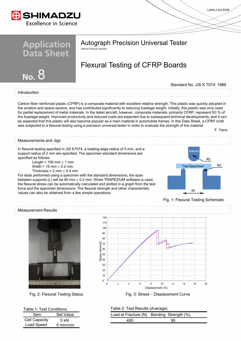
8 Flexural Testing of CFRP Boards
LAAN-J-AG-E008
Material Testing & Inspection
Standard No. JIS K 7074: 1988
Introduction
Measurement Results
Measurements and Jigs
Carbon fiber reinforced plastic (CFRP) is a composite material with excellent relative strength. This plastic was quickly adopted in the aviation and space sectors, and has contributed significantly to reducing fuselage weight. Initially, this plastic was only used for partial replacement of metal materials. In the latest aircraft, however, composite materials, primarily CFRP, represent 50 % of the fuselage weight. Improved productivity and reduced costs are expected due to subsequent technical developments, and it can be expected that this plastic will also become popular as a main material in automobile frames. In this Data Sheet, a CFRP clothwas subjected to a flexural testing using a precision universal tester in order to evaluate the strength of the material.
F. Yano
Fig. 1: Flexural Testing Schematic
支持台
Indenter
Test Specimen
D
R5
R2
80
In flexural testing specified in JIS K7074, a loading edge radius of 5 mm, and a support radius of 2 mm are specified. The specimen standard dimensions are specified as follows:
Length = 100 mm 1 mmWidth = 15 mm 0.2 mmThickness = 2 mm 0.4 mm
For tests performed using a specimen with the standard dimensions, the span between supports (L) will be 80 mm 0.2 mm. When TRAPEZIUM software is used, the flexural stress can be automatically calculated and plotted in a graph from the test force and the specimen dimensions. The flexural strength and other characteristic values can also be obtained from a few simple operations.
Fig. 2: Flexural Testing Status Fig. 3: Stress – Displacement Curve
Stre
ss (N
/mm
2)
Displacement (%)
Table 2: Test Results (Average)Load at Fracture (N) Bending Strength (%)
485 95
Table 1: Test ConditionsItem Set Value
Cell Capacity 5 kNLoad Speed 5 mm/min
Autograph Precision Universal Tester

8
First Edition: February 2013
© Shimadzu Corporation, 2013www.shimadzu.com/an/
Shimadzu Corporation
CFRP Flexural Testing System
Tester: AG-XplusLoad Cell: 5 kNTest Jig: Three-point bending test jig for plasticsSoftware: TRAPEZIUM X (Single)
AGS-X Table-Top Precision Universal Tester
A high-precision load cell is adopted. (The high-precision type is class 0.5; the standard-precision type is class 1.)Accuracy is guaranteed over a wide range, from 1/1000 to 1/1 of the load cell capacity. This supports highly reliable test evaluations.
Crosshead speed rangeTests can be performed over a wide range from 0.0005 mm/min to 1,500 mm/min.
High-speed samplingUltrafast sampling, as fast as 0.2 msec. Sudden changes in test force, such as when brittle materials fracture, can be assessed.
TRAPEZIUMX operational softwareDesigned for intuitive operation, this software offers excellent convenience and user friendliness.
Smart controllerReal-time test force and position data is readily confirmed, and the manual dial can be used for fine adjustments to jig positioning.
Optional Test DevicesA variety of tests can be conducted by switching between an abundance of jigs in the lineup.
Features
AG-Xplus Table-Top Precision Universal Tester

16
LAAN-J-AG0016
Material Testing & Inspection
Autograph Precision Universal Tester
Measurement Results
In this test, the test sample is fixed to a test specimen mounting board made from a paper, metal, or resin sheet as shown in Fig. 1, installed in the grips, and the tensile test is performed. The standard describes in detail the shape of the mounting board, the type of adhesive used to fix the carbon fiber to the mounting board, and the procedure for installing the carbon fiber (for details refer to the standard). The tests were carried out using clip type grips whose grip force could be adjusted in accordance with the strength of the sample.
Measurements and Jigs
Carbon fiber is an important industrial material, being essential in carbon fiber reinforced plastics (CFRP), having a specific gravity one-fourth that of normal steels, and a specific strength of 7 times. In this Application Data Sheet, examples of tensile testing of single carbon fibers based on the ISO standard are introduced.
T. Murakami
Introduction
Standard No. ISO11566: 1996 (JIS R 7606: 2000)
Fig. 1 Test Sample and Mounting Board (frame)
Single carbon fiber
Position for cutting mounting board Adhesive
Sample Diameter Tensile Strength Elongation at Break
Carbon fiber 6 m 7.1 GPa 2.84 %
Table 2 Test Results (average)
Fig. 2 Test Status
Tensile Testing of Carbon Fiber
Fig. 3 Test Results
Stre
ss (G
Pa)
Strain (%)
Table 1 Test Conditions
Item Set Value Test speed 1 mm/minDistance between grips 25 mm

16
First Edition: February 2013
© Shimadzu Corporation, 2013www.shimadzu.com/an/
Shimadzu Corporation
High Accuracy Displacement MeasurementA high accuracy (0.2 m) linear sensor has been adopted for measurement of displacement in the load direction. In addition, the backlash-free structure makes it possible to carry out testing with good accuracy.Displacement in the load direction of the test sample can be set accurately to a displacement display resolution of 0.02 m and a control resolution of 0.005 m.
Measurement of Micro Test ForcesA wide range of load cells from 0.5 N to 2 kN assures a precision of 1 % for measurements of testing forces of 2 mN at minimum.
Positioning Very Small Test SamplesUsing an X-Y stage (optional), very small test samples can be easily positioned.The position of the test samples can be observed using a stereo microscope.
High Rigidity FrameA high rigidity frame (45 kN/mm minimum) has been adopted to enable measurement of minute displacements.
Optional Test DevicesA variety of tests can be accommodated by switching between an abundance of jigs in the lineup.
Features
Shimadzu Autograph MST-1 Micro Strength Evaluation Testing Machine
Carbon Fiber Tensile Test System
Tester: MST-I Type HRLoad Cell: 1 N Test Jig: 1 N clip type grips (rubber-coated teeth), X-Y stage Software: TRAPEZIUM X (Single)

■
■
≈ σ τ στ


■

■
■

■
■
× × ×
■

① ②
① ② ③ ④
⑤ ⑥ ⑦ ⑧
⑨ ⑩ ⑪ ⑫

① ② ③ ④
⑤ ⑥ ⑦ ⑧
⑨ ⑩ ⑪ ⑫

■
www.shimadzu.com/an/
Shimadzu Corporation
First Edition: July, 2015

Results

(1) (2) (3) (4)
(5) (6) (7) (8)
(9) (10) (11) (12)
www.shimadzu.com/an/
Shimadzu Corporation
First Edition: July, 2015

Specimen NameOpen-Hole Compressive
Strength
1st 278.2 MPa
2nd 273.0 MPa
Mean 275.6 MPa
ApplicationNews
No.i256
Material Testing System
Open-Hole Compression Test of Composite Material
LAAN-A-AG-E020
Introduction
Carbon fiber reinforced plastic (CFRP) has gained attention due to their strength and low weight, and have quickly been adopted for use in aeronautics and astronautics. CFRP has excellent strength characteristics in terms of specific strength and high rigidity, but lose much of their strength when a cutout is made. Consequently, composite materials used in aeroplanes must be evaluated by tests that use specimens with a hole cut out of their center. We performed open-hole compression testing of a CFRP according to ASTM D6484.
Measurement System
The CFRP spec imen used was T800S/3900. As shown in Fig. 1, a hole was created in the middle of the spec imen. ASTM D6484 descr ibes tes t methods in both SI and Imperial units, where the dimensions of the j igs and specimens differ in each. We performed testing with Imperial units. Specimen information is shown in Table 1.ASTM D6484 inc ludes two load ing methods , which are described as Method A and Method B. In Method A, the specimen and test f ixture are clamped in a gripping device, and the specimen is compressed by shear force applied by the fixture and gripping device. In Method B, compression plate is present at the ends of the specimen and fixture, and are used to compress the specimen. Method B was used, as shown in Fig. 2. Table 2 shows a l ist of the equipment used and Table 3 shows the test conditions used.
Length : 30 mmWidth : 38.1 mmThickness : 3.1 mmLamination Method : [45/0/–45/92] 2S
Table 1 Specimen Information
Fig. 1 Specimen
Fig. 2 Test Setup
Testing Machine : AG-XplusLoad Cell : 50 kNTest Fixture : Open-Hole Compression Test Fixture
Table 2 Experimental Equipment
Test Speed : 2 mm/min
Table 3 Test Conditions
ResultsMeasurements were performed twice. Test results are shown in Table 4 and stress-displacement curves are shown in Fig. 3. As shown in Table 4, the mean open-hole compressive strength was 275.6 MPa.
Table 4 Test Results

0
0
20
40
6080
100
120
140
160
180
200
220240
260
280
300
0.2 0.4 0.6 0.8 1 1.2
Displacement (mm)
Str
ess
(N
/mm
2)
1.4 1.6 1.8 2 2.2 2.5
ApplicationNews
No.
© Shimadzu Corporation, 2016
For Research Use Only. Not for use in diagnostic procedure.
This publication may contain references to products that are not available in your country. Please contact us to check the availability of these
products in your country.
The content of this publication shall not be reproduced, altered or sold for any commercial purpose without the written approval of Shimadzu.
Company names, product/service names and logos used in this publication are trademarks and trade names of Shimadzu Corporation or its
affiliates, whether or not they are used with trademark symbol “TM” or “®”. Third-party trademarks and trade names may be used in this
publication to refer to either the entities or their products/services. Shimadzu disclaims any proprietary interest in trademarks and trade names
other than its own.
The information contained herein is provided to you "as is" without warranty of any kind including without limitation warranties as to its
accuracy or completeness. Shimadzu does not assume any responsibility or liability for any damage, whether direct or indirect, relating to the
use of this publication. This publication is based upon the information available to Shimadzu on or before the date of publication, and subject
to change without notice.
www.shimadzu.com/an/
i256
First Edition: Aug. 2016
Fig. 3 Stress-Displacement Curves
Results (DIC Analysis)
Using the TRViewX non-contact extensometer allows for images and video of the specimen to be collected synchronized with test result col lect ion. Also, applying a random pattern of paint to the observed specimen surface allows the images or video to be used to determine the strain distribution on the observed specimen surface during the test by DIC analysis1). Open-hole compression testing and DIC ana lys i s were per formed us ing the spec imen described in Table 5. Fig. 4 shows a photograph of the open-hole compression test system with a non-c o n t a c t e x t e n s o m e t e r. F i g . 5 s h o w s s t r a i n distributions around the open hole in the specimen that were obtained by DIC analysis. Fig. 5 shows that strain accumulates at the vertical sides of the open hole (regions (1) and (3)), strain appears along the axis of compression from those points, and the final break occurs at the vert ica l s ides of the hole. Meanwhile, almost no strain appears in the central part of the hole (region (2)) throughout the test. This strain distribution probably occurred due to a 0˚ fiber orientation on the surface of the specimen.
Length : 30 mmWidth : 38 mmThickness : 1.6 mmLamination Method : [0/90] 2S
Table 5 Specimen Information (DIC)
1) DIC analysis is an analysis method that measures strain and showsthe strain distribution in a specimen based on movement of arandom pattern of paint applied to the observed specimen surfacebefore and during testing.
Fig. 4 Experimental Setup (DIC)
①②③
1 2 3
4 5 6
Fig. 5 DIC Analysis Results
Conclusion
Using this test system, open-hole compression testing of a CFRP was successfully performed according to ASTM D6484. Using a non-contact extensometer, we were also able to capture video (images) synchronized with the test force and crosshead displacement data obtained from the testing machine. Performing DIC analysis based on this video allowed an evaluation of the strain distribution on the observed specimen surface. This testing system will be extremely useful for the development of CFRPs and products that use CFRPs.
Edition: . 2016

ApplicationNews
No.i250
Material Testing System
Shear Test of Composite Material
(V-Notched Beam)
LAAN-A-AG-E015
Introduction
Carbon fiber reinforced plastic (CFRP) do not oxidize or rust and have a higher specific strength and stiffness than existing materials. Applications of CFRP are being investigated, with a focus on applications as industrial products that require strength and durability. Compared to exist ing homogeneous materials, composite materials like CFRP are anisotropic, and display complex failure behaviors as a result of tension, compression, bending, in-plane shear, out-of-plane shear, or a combination of these stresses arising from loading in the principal-axis direction. In recent years, use of CAE analysis in industry has become widespread since it can reduce numbers of prototypes and reduce the cost of new product development. Because values for each of the stress properties stated above are needed to i n c rea se p re c i s i on when p red i c t i ng p roduc t characteristics during product design, there is a strong demand for test methods able to evaluate pure failure behaviors in CFRP.This article describes an example of V-notched beam method (Iosipescu method, ASTM D5379) that is widely used as an in-plane shear test method for composite material specimens. The test method can apply load as a pure in-plane shear stress on the evaluation area (see Fig. 1) by using a specimen cut with V-notches and supported at four asymmetrical points. Setting up the specimen and jig for this test method is relatively easy, and the test method can be used with a variety of CFRP laminate materials, including unidirectional materials, orthogonally laminated materials, and discontinuous fiber materials.
Measurement System
The equipment configuration is shown in Table 1. Information on the specimen prescribed by ASTM D5379 is shown in Fig. 1. The specimen is a [0/90]10s
orthogonally laminated material made from Toray T800S prepreg that was molded in an autoclave. A two-axis strain gauge was attached at the mid-point between the upper and lower V-notches machined into the specimen (evaluation area), and oriented to measure strain in –45˚ and +45˚ directions. Shear strain can be calculated by inserting the strain values obtained from these two strain gauges into equation (1). Shear strain is a property needed to evaluate the shear modulus. In this test, strain gauges were attached on both the front and rear of the specimen. Calculating the mean of outputs obtained from strain gauges on both sides allows for more accurate measurement of the shear strain in the specimen, and confirms whether shear strain is being applied symmetrically on the front and rear of the specimen.
. Equation (1)
: Shear strain
: Strain at +45˚
+45 +=ε –45εγγ
+45ε: Strain at –45˚–45ε
Testing Machine : AG-50kNX plusLoad Cell : 50 kNTest Jig : ASTM D 5379 jigSoftware : TRAPEZIUM X (Single)Test Speed : 2 mm/min
Table 1 Test Conditions
Fig. 2 Testing Apparatus
Fig. 3 Imaging Apparatus
Evaluationarea
90˚
19
.05
11
.43
76.2
Fig. 1 Shape of Specimen

ApplicationNews
No.i250
The testing and imaging apparatus are shown in Fig. 2 and 3. Images captured using a TRViewX (Sh imadzu D ig i ta l V ideo Ex tensometer ) were gathered simultaneous to values obtained from the strain gauge outputs and specimen stress obtained by the test ing apparatus. This made it easy to compare and evaluate images of the CFRP failure process against each specimen property values, something that was difficult to perform only with previous testing systems. Strain distribution can also be evaluated using digital image correlation (DIC, ARAMIS, GOMmbH) analysis of the images captured by TRViewX. To perform DIC analysis, paint must be sprayed on the specimen surface to create a random pattern on the front surface of the specimen.
Analytical Results
Each specimen property value obtained from this test is shown in Table 2. A photograph of the specimen after testing is shown in Fig. 4, a shear stress-normal strain curve is shown in Fig. 5 (strain values obtained from strain gauges), a shear stress-shear strain curve is shown in Fig. 6 (shear strain calculated from Equation (1)), and a shear stress-stroke curve is shown in Fig. 7. Table 2 shows that the results obta ined for each shear property were h ighly reproducible. Fig. 5 and Fig. 6 show that the same strain values were obtained from the front and rear strain gauges, and highly symmetrical shear strain was applied to the specimen.
Table 2 Test Results
SpecimenShear Modulus
[GPa]
Shear Strength
[MPa]
Test 1 4.62 136.0
Test 2 4.63 133.0
Test 3 4.50 131.0
Mean 4.58 133.0
Plastic deformationcaused by shearing
Fig. 4 Specimen After Testing
-6 -5 -4 -3 -2 -1 0 1 2 3 4 5 60
10
20
30
40
50
60
70
80
90
100
Back +45 ˚Front +45 ˚
Back –45 ˚Front –45 ˚
Shear
Str
ess
(M
Pa)
Strain (%)
Fig. 5 Shear Stress-Normal Strain Curve
0 1 2 3 4 5 6 7 8 9 100
10
20
30
40
50
60
70
80
90
100
BackFront
Sh
ear
Str
ess
(M
Pa)
Shear Strain (%)
0.0 0.5 1.0 1.5 2.0 2.5 3.0 3.5 4.0 4.5 5.0 5.5 6.00
10
20
30
40
50
60
70
80
90
100
110
120
130
140
Sh
ear
Str
ess
(M
Pa)
Stroke (mm)
Max
Fig. 6 Shear Stress-Shear Strain Curve
Fig. 7 Shear Stress-Stroke Curve
Failure of the specimen is shown in Fig. 8. Images of the shear strain distribution obtained by DIC analysis are shown in Fig. 9. The amount of strain occurring in the specimen is shown in terms of color, with low strain areas in cooler colors (black and blue) and high strain areas in warmer colors (orange and red). The images show that as the test progresses strain accumulates and is localized between the V-notches.

ApplicationNews
No.i250
① ② ③ ④ ⑤Fig. 8 Specimen e Failure Process (images show the point at which the specimen fails)
① ② ③
④ ⑤ ⑥
⑦ ⑧ ⑨
Fig. 9 Shear Strain Distribution (DIC analysis images)

ApplicationNews
No.
© Shimadzu Corporation, 2016
For Research Use Only. Not for use in diagnostic procedure.
This publication may contain references to products that are not available in your country. Please contact us to check the availability of these
products in your country.
The content of this publication shall not be reproduced, altered or sold for any commercial purpose without the written approval of Shimadzu.
Company names, product/service names and logos used in this publication are trademarks and trade names of Shimadzu Corporation or its
affiliates, whether or not they are used with trademark symbol “TM” or “®”. Third-party trademarks and trade names may be used in this
publication to refer to either the entities or their products/services. Shimadzu disclaims any proprietary interest in trademarks and trade names
other than its own.
The information contained herein is provided to you "as is" without warranty of any kind including without limitation warranties as to its
accuracy or completeness. Shimadzu does not assume any responsibility or liability for any damage, whether direct or indirect, relating to the
use of this publication. This publication is based upon the information available to Shimadzu on or before the date of publication, and subject
to change without notice.
www.shimadzu.com/an/
i250
First Edition: Aug. 2016
Conclusion
We used this test system to successfully implement the V-notched beam method (ASTM D5379). In addition to evaluating the basic properties of shear modulus and shear strength, integrating a Digital Video Extensometer into the test system enabled us to capture reference data that can be used to elucidate the mechanism of failure of CFRP, allowing strain analysis to be performed in terms of specimen failure mode and DIC analysis.

ApplicationNews
No.i251
Material Testing System
Shear Test of Composite Material
(V-Notched Rail Shear)
LAAN-A-AG-E016
Introduction
Carbon fiber reinforced plastic (CFRP) do not oxidize or rust and have a higher specific strength and stiffness than existing materials. Applications of CFRP are being investigated, with a focus on applications as industrial products that require strength and durability. Compared to exist ing homogeneous materials, composite materials like CFRP are anisotropic, and display complex failure behaviors as a result of tension, compression, bending, in-plane shear, out-of-plane shear, or a combination of these stresses arising from loading in the principal-axis direction. In recent years, use of CAE analysis in industry has become widespread since it can reduce numbers of prototypes and reduce the cost of new product development. Because values for each of the stress properties stated above are needed to i n c rea se p re c i s i on when p red i c t i ng p roduc t characteristics during product design, there is a strong demand for test methods able to evaluate pure failure behaviors in CFRP.There are various tests methods for evaluating composite materials. Of these methods, two commonly used in-plane shear test methods to test in the direction of fibers in fiber reinforced composite materials and to test textile laminated materials are the Iosipescu method (ASTM D5379) that applies an asymmetrical four-point bending load to a specimen cut with notches, and method (ISO 14129) that applies a ±45˚ tensile load on laminated materials. We used the V-notched rail shear method (ASTM D7078) that can be used to test in-plane shear. Because this method uses a large gauge area on the specimen, it can accommodate specimens without holes and CRFP laminate materials that have discontinuous fibers.
Measurement System
The equipment configuration is shown in Table 1. Information on the specimen prescribed by ASTM D7078 is shown in F ig. 1. The specimen is a [0/90]10s orthogonally laminated material made from Toray T800S prepreg that was molded in an autoclave. The specimen has a 31-mm evaluation area (see Fig. 1), and two-axis strain gauges attached at the mid-point between the V-notches (center of evaluation area) that are able to measure strain in –45˚ and +45˚ directions. Shear strain can be calculated by inserting the strain values obtained from these two strain gauges into equation (1). Shear strain is a property needed to evaluate the shear modulus.
. Equation (1)
: Shear strain
: Strain at +45˚
+45 +=ε –45εγγ
+45ε: Strain at –45˚–45ε
In this test, strain gauges were attached on both the front and rear of the specimen. Calculating the mean of outputs obtained from strain gauges on both sides allows for more accurate measurement of the shear strain in the specimen, and confirms whether shear
strain is being applied symmetrically on the front and rear of the specimen.
Testing Machine : AG-50kNX plusLoad Cell : 50 kNTest Jig : ASTM D7078 jigSoftware : TRAPEZIUM X (Single)Test Speed : 2 mm/min
Table 1 Test Conditions
Strain gauge
90˚
31
.0
56
.0
76.0
in gaugen gaugin
9090
aiStra
Evaluation area
Fig. 1 Shape of Specimen
Fig. 2 Testing Apparatus
Fig. 3 Imaging Apparatus

ApplicationNews
No.i251
The testing and imaging apparatus are shown in Fig. 2 and Fig. 3. Images captured using a TRViewX (Shimadzu Digital Video Extensometer) were gathered simultaneous to values obtained from the strain gauge outputs and specimen stress obtained by the testing apparatus. This made it easy to compare and evaluate images of the CFRP failure process against each specimen property values, something that was difficult to perform only with previous testing systems. Strain distribution can also be evaluated using digital image correlation (DIC, ARAMIS, GOMmbH) analysis of the images captured by TRViewX. To perform DIC analysis, paint must be sprayed on the specimen surface to create a random pattern on the front surface of the specimen.
Analytical Results
Each specimen property value obtained from this test is shown in Table 2. A photograph of the specimen after testing is shown in Fig. 4, a shear stress-normal strain curve is shown in Fig. 5 (strain values obtained from strain gauges), a shear stress-shear strain curve is shown in Fig. 6 (shear strain calculated from Equation (1)), and a shear stress-stroke curve is shown in Fig. 7. Table 2 shows that the results obta ined for each shear property were h ighly reproducible. Fig. 5 and Fig. 6 show that the same strain values were obtained from the front and rear strain gauges, and highly symmetrical shear strain was applied to the specimen.
Table 2 Test Results
Specimen Shear Modulus
[GPa]
Shear Strength
[MPa]
Test 1 4.63 121.72
Test 2 4.55 120.00
Test 3 4.58 120.05
Mean 4.59 120.60
Plastic deformationcaused by shearingPcc
Fig. 4 Specimen After Testing
-6 -5 -4 -3 -2 -1 0 1 2 3 4 5 6
10
20
30
40
50
60
70
80
90
100
Back +45˚Front +45˚
Back –45˚Front –45˚
Strain (%)
Sh
ear
Str
ess
(M
Pa)
0
Fig. 5 Shear Stress-Normal Strain Curve
0 1 2 3 4 5 6 7 8 9 100
10
20
30
40
50
60
70
80
90
100
BackFront
Sh
ear
Str
ess
(M
Pa)
Shear Strain (%)
Fig. 6 Shear Stress-Shear Strain Curve
0.0 0.5 1.0 1.5 2.0 2.5 3.0 3.5 4.0 4.5 5.0 5.5 6.00
10
20
30
40
50
60
70
80
90
100
110
120
130
140
Sh
ear
Str
ess
(M
Pa)
Stroke (mm)
Max
Fig. 7 Shear Stress-Stroke Curve
Failure of the specimen is shown in Fig. 8. A crack that appears c lose to the upper notch quickly propagates down toward the bottom notch during a simultaneous decrease in test force. Images of the shear strain distribution obtained by DIC analysis are shown in Fig. 9. The amount of strain occurring in the specimen is shown in terms of color, with low strain areas in cooler colors (black and blue) and high strain areas in warmer colors (orange and red). The images show that as the test progresses strain accumulates and is localized between the V-notches.

ApplicationNews
No.i251
Fig. 8 Specimen Failure Process (images show the point at which the specimen fails)
① ② ③ ④ ⑤
⑥ ⑦ ⑧ ⑨ ⑩
⑪ ⑫ ⑬ ⑭ ⑮Fig. 9 Shear Strain Distribution (DIC analysis images)

ApplicationNews
No.
© Shimadzu Corporation, 2016
For Research Use Only. Not for use in diagnostic procedure.
This publication may contain references to products that are not available in your country. Please contact us to check the availability of these
products in your country.
The content of this publication shall not be reproduced, altered or sold for any commercial purpose without the written approval of Shimadzu.
Company names, product/service names and logos used in this publication are trademarks and trade names of Shimadzu Corporation or its
affiliates, whether or not they are used with trademark symbol “TM” or “®”. Third-party trademarks and trade names may be used in this
publication to refer to either the entities or their products/services. Shimadzu disclaims any proprietary interest in trademarks and trade names
other than its own.
The information contained herein is provided to you "as is" without warranty of any kind including without limitation warranties as to its
accuracy or completeness. Shimadzu does not assume any responsibility or liability for any damage, whether direct or indirect, relating to the
use of this publication. This publication is based upon the information available to Shimadzu on or before the date of publication, and subject
to change without notice.
www.shimadzu.com/an/
i251
First Edition: Aug. 2016
Conclusion
We used this test system to successfully implement the V-notched rail shear method (ASTM D7078). In addition to evaluating the basic properties of shear modulus and shear strength, integrating a Digital Video Extensometer into the test system enabled us to capture reference data that can be used to elucidate the mechanism of failure of CFRP, allowing strain analysis to be performed in terms of specimen failure mode and DIC analysis.

■ Introduction As the result of recent progress of research and development, carbon fiber materials have been put to practical use in a wide range of implements, including space aircraft parts, sporting goods like golf club shafts and tennis rackets, structure materials that must transmit X-rays, and acoustic materials. A group of high-quality carbon fibers is further classified, according to its tensile strength, into several groups. One of these is a high-strength fiber group that features in excellent tensile strength; another is a high-elasticity fiber group characterized by high flexibility, but with a tensile strength of no more than around 2,000 MPa. As described above, data on mechanical properties are indispensable information for classifying fibers. The following is an example of tests for evaluation of physical behaviors under a compressive force applied to carbon fibers (single fibers) having different tensile strength levels with Shimadzu Micro Compression Testing Machine MCT.
■ Testing Conditions (1) Testing mode: compression test (2) Testing load: 200 gf (3) Loading rate constant: 1 (4,230 gf/sec.) (4) Calculation of strength: Compression strength is calculated by the following equation. *1
𝑆𝑆𝑆𝑆𝑆𝑆𝑆𝑆 = 2 ∙ 𝑃𝑃𝑃𝑃 ∙ 𝜋𝜋𝜋𝜋 ∙ 𝑑𝑑𝑑𝑑 ∙ 𝐿𝐿𝐿𝐿
where: ST: tensile strength (kg/mm2) P: compression strength (kgf) d: diameter of fiber (mm) L: length of fiber (mm) Note *1: from JIS A1113-1976 Method of tests for splitting tensile strength of concrete
Material Testing System MCT
Compression-Rupture Test of Carbon Fibers with Different Tensile Characteristics Shimadzu Micro Compression Testing
No. SCA_300_037
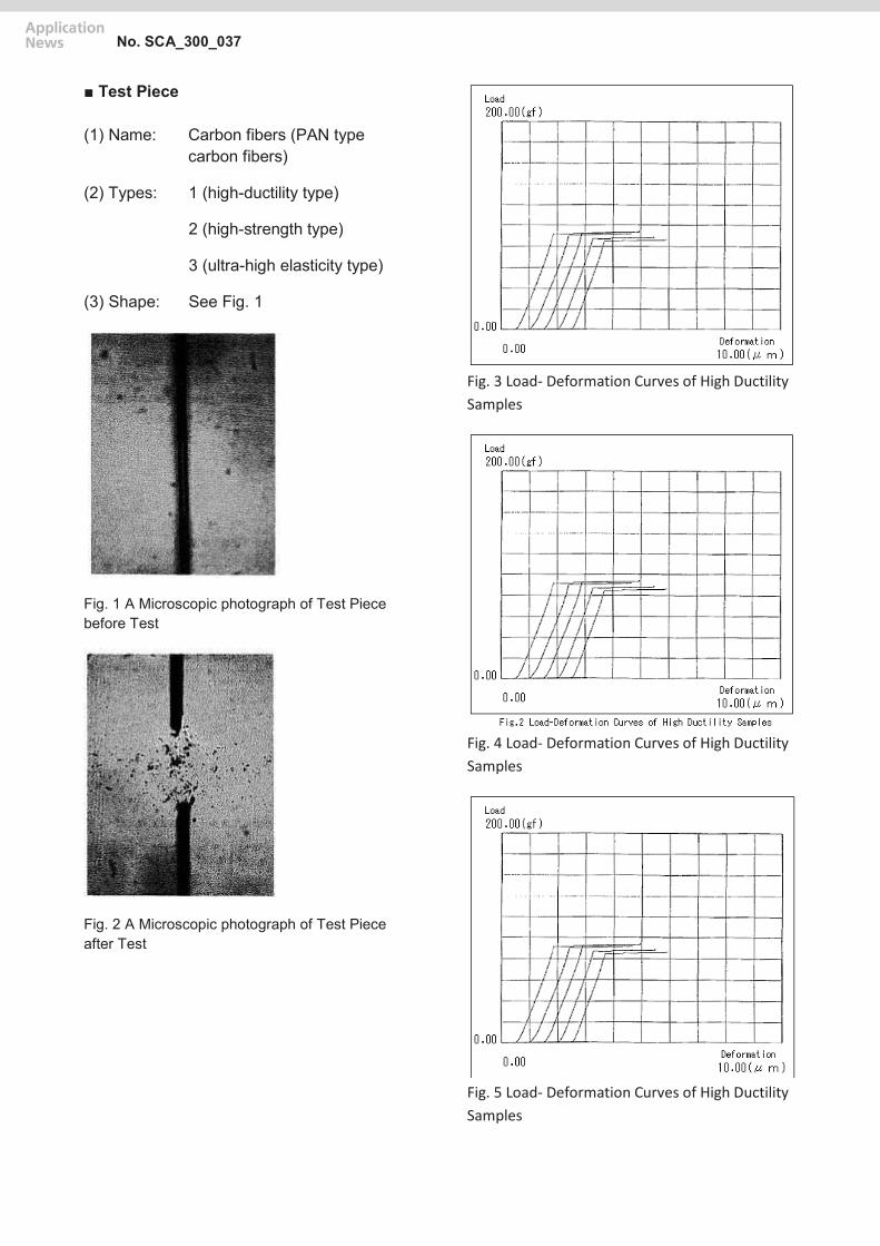
■ Test Piece (1) Name: Carbon fibers (PAN type
carbon fibers)
(2) Types: 1 (high-ductility type)
2 (high-strength type)
3 (ultra-high elasticity type)
(3) Shape: See Fig. 1
Fig. 1 A Microscopic photograph of Test Piece before Test
Fig. 2 A Microscopic photograph of Test Piece after Test
Fig. 3 Load- Deformation Curves of High Ductility Samples
Fig. 4 Load- Deformation Curves of High Ductility Samples
Fig. 5 Load- Deformation Curves of High Ductility Samples
No. SCA_300_037

Type of test piece Compression-rupture strength(kgf/mm2)
Standard deviation (kgf/mm2)
High-ductility type 149.90 3.23 High-strength type 151.09 6.34 Ultra-high elasticity type 68.87 4.37
Table 1 Results of Compression-Rupture Test of Carbon Fibers
Note: The length of the indenter diameter (50 mm) was used for the length of fiber because the test piece was extraordinarily long.
■ Test Results Table 1 shows a summary of test data, and Figs. 2-4 show the compression-rupture strength and the overlapping view of load-deformation curves for each test piece. The difference of behavior between test pieces are observable in the load-deformation curves of Figs. 2-4. The test pieces of the high-ductility type and the high-strength type have similar compression-rupture strength, while the ultra-high elasticity type has a remarkably low compression-rupture strength. (Refer to Table 1) Admitting some deviation among the test data as a result of the surface conditions of the test pieces, the test results ensure that this testing machine is useful and effective for evaluation of mechanical properties of single fibers, provided that data are processed statistically. * Please be advised that data obtained before the implementation of the current Weights and Measures Law may be presented in terms of gravimetric unit.
No. SCA_300_037

CFRP (carbon fiber reinforced plastic) has attracted attention as a high-performance composite material with high strength and rigidity, yet low in weight, and is being applied in various fields, such as for aircraft, railroad vehicles, automobiles and civil engineering. This example describes evaluating the characteristics of a flat plate specimen of CFRP material when a tensile load is applied (tensile test) and observing the fracture status. Tensile testing consisted of static testing of material strength and measuring the modulus of elasticity using a precision universal testing machine. In addition, high-rate tensile impact test was also performed. In the latter case, a high-speed video camera was used to record specimen fracture, which allowed capturing image data of the instant the CFRP material fractured. ■ Test specimen The tensile test specimen tested in this example is shown in figure 1. Included 50 mm long CFRP tabs attached to both ends of the CFRP strip with thermosetting resin adhesive. Reinforcing the grip area with tabs ensures a stable tensile test with good reproducibility.
Figure 1: CFRP test specimen
Specimen details are as follows: 1) Material: unidirectional CFRP 2) Shape: strip (with tabs on both ends) 3) Specimen dimensions: for static tensile
testing 200(L) x 12.5(W) x 1(T) mm. For recording image of impact fracture 70(L) x 6.25(W) x 0.3(T) mm
■ Static tensile test A strain gauge type extensometer was attached to the specimen and a tensile test was performed using a precision testing machine. The extensometer was removed when strain exceeded the elasticity measurement range. It is also possible to measure strain by affixing a strain gauge instead of an extensometer. Tensile test parameters are indicated below. (1) Tensile rate: 10 mm/min (2) Grip distance: 100 mm (3) Test force detection: 50 KN load cell (4) Extensometer gauge length: 50 mm (5) Elasticity calculation range: 5/10,000 to
25/10,000 strain
Figure 2: Static test results
Material Testing System AG-X
Observation of fracture in CFRP tensile test
No. SCA_300_059

The elasticity of CFRP specimen can be determined by calculating the slope of the given strain region (elasticity calculation range) in the stress-strain curve (figure 2) obtained from test results. Tensile strangth can be determined from the maximum stress in the stress-displacement curve (figure 3) before the specimen breaks.
Figure 3: Static test results
The following values were obtained from the measurement data. (1) Tensile strength: 346 GPa (2) Elasticity: 148 GPa
The post-test status of the specimen is shown in figure 4. Compared to the starting status in figure 1, it clearly shows how the fibers within the resin have failed.
Figure 4: Specimen status after static test
■ Static tensile test To verify functionality, development of composite materials involves not only static Static strength testing, but also involves the objective of ensuring active safety. Consequently, it is important to determine the shock strength and understand the process of fracture propagation. Therefore, the fracture process during tensile chock testing of a CFRP specimen was observed by combining a high-speed video camera with high-rate tensile shock test machine. Observation conditions are indicated below. Specimen tensile rate: 6 m/s
Grip distance: 30 mm
Camera lens: 105 mm macro, with 2 x teleconverter
Camera lighting: strobe
Camera trigger:
signal synchronized with tensile displacement is sent from testing machine to camera.
The setup used to record video of the test is shown in figure 5, with a high-speed video camera mounted about 450 mm in front of the specimen. Recording was activated by an external start trigger signal sent from the testing machine to the camera, which was synchronized to the tensile displacement. A strobe light synchronized to the video timing was used as lighting.
Figure 5: Setup of high-rate shock test
No. SCA_300_059

Using this test configuration, a load was applied to the CFRP specimen according to the parameters indicated above and a high-speed camera captured the instant of fracture, at 250.000 frames per second. This image data shown in figure 6. This shows 8 consecutive frames, from (1) TO (8), with an interval of 4 microseconds between each frame. This camera features highly detailed image resolution of 312
horizontal by 260 vertical pixels that is constant, regardless of the frame rate. This example shows, combining a high-speed video camera and material testing machine makes it possible to evaluate material properties and observe fracture behavior at the same time. This enables supporting a wide range of material development applications, from developing individual functionally enhanced resins to developing composite materials.
Figure 6: Images of specimen during fracture
No. SCA_300_059

C225-E032
Ultrasonic Fatigue Testing System Effective for Gigacycle Fatigue Tests
With fatigue tests of high-strength steels, it is evident that internal fracture (fish-eye fracture), which is caused by inclusions and other micro defects, occurs at 107 cycles or more, a value considered the conventional fatigue limit.An ultrasonic fatigue testing system is extremely effective when performing this sort of gigacycle fatigue test. (With a 100 Hz fatigue testing system, this would take 3 years, but if a 20 kHz ultrasonic fatigue testing system is used, testing can be completed in one week.)
Actual components are rarely used under conditions in which the average stress is zero. Despite this, the USF-2000A, a standard ultrasonic fatigue testing system, can only perform testing under zero average stress conditions.Using an ultrasonic fatigue testing system equipped with an average stress loading mechanism, gigacycle fatigue tests can be performed with average tensile stress loaded.
Ultrasonic Fatigue Testing System with an Average Stress Loading Mechanism
Stressdistribution
AG-X5kNAverage stress loading
High-rigidity booster
Horns
High-rigidity booster
5 kN load cellAverage stress measurement
Converter(Piezo actuator)
Strain GaugeSamples
DisplacementStress
System Appearance
For Gigacycle Fatigue Tests with Average Stress Loaded

© Shimadzu Corporation, 2016First Edition: August 2016
For Research Use Only. Not for use in diagnostic procedure. This publication may contain references to products that are not available in your country. Please contact us to check the availability of these products in your country.Company names, product/service names and logos used in this publication are trademarks and trade names of Shimadzu Corporation or its affiliates, whether or not they are used with trademark symbol “TM” or “®”. Third-party trademarks and trade names may be used in this publication to refer to either the entities or their products/services. Shimadzu disclaims any proprietary interest in trademarks and trade names other than its own.
The contents of this publication are provided to you “as is” without warranty of any kind, and are subject to change without notice. Shimadzu does not assume any responsibility or liability for any damage, whether direct or indirect, relating to the use of this publication.www.shimadzu.com/an/
Ultrasonic resonance systemPower supply, converter, booster (1 pair), horn (1 pair)
Personal computer(OS Windows 7) ADA/PIO interface board
SoftwareUltrasonic test control measurement software
Cooling systemAir dryer, air piping• A separate 140 L/min air source is required.
5 Strain meter unit (option)
6 AG-X plus Autograph 5 kN + 250 extension
7 Average stress loading mechanism
1
2
3
4
Main Speci�cations
1) Test Frequency: 20 kHz ± 500 Hz
• The recommended test range is 20 kHz ± 30 Hz.• The test frequency is determined by the resonance frequency of the sample.
2) Horn End Face Amplitude
Min. approx. ±10 μmMax. approx. ±50 μm
• The minimum and maximum amplitudes are the end face amplitude values at amplitude outputs of 20 % and 100 % respectively. Accordingly, the minimum and maximum amplitude values will change somewhat depending on the shape of the sample.
4) Average Stress
Max. 1.5 kN (tensile only)
3) Test Stress
Standard circular tapered sampleStress Min. 237 MPa Max. 1186 MPa• The test stress range can be changed by changing the sample shape.• The minimum and maximum values are calculated with the end face amplitude values of 10 μm and 50 μm respectively.• These are the values when the stress is within the elasticity range.
Standard Circular Tapered Sample
Surface of the Fatigued Fracture Originating from the Inclusion
Center hole can remain
Center holecan remain
Components

ApplicationNews
No.
LAAN-A-AG-E009
Material Testing System
Tensile Test for Metallic Materials Using Strain Rate Control and Stress Rate Control
i244International standards for tensile testing of metallic materials have been revised as specified in ISO 6892 and JIS Z2241, such that strain rate control, where strain is measured with an extensometer, has recently been added as a test item to the current stress rate control method, in which a load is applied to a material until its yield point is reached. As a result, it can be assumed that there will be situations where both stress rate control and strain rate control tensile testing of
metallic materials will be required.Here, we introduce examples of strain rate control and stress rate control tensile testing of metallic samples, including cold-rolled steel, austenitic stainless steel, aluminium alloy and brass, according to ISO 6892, using the Shimadzu Autograph AG-50kNX Precision Universal Tester, and the SSG50-10H strain gauge type one-touch extensometer (Fig. 1, Fig. 2).
Table 1 Test Specimens
Information on the sample specimens are shown in Table 1, and the test conditions are shown in Table 2.
n Introduction
n Specimens and Test Conditions
Fig. 1 Overview of Universal Testing System Fig. 2 Specimen and Jigs for Tensile Testing
Sample Name A B C D
Material Cold-rolled steel Stainless steel (austenitic) Aluminium alloy Brass
Sample size
Width 25 mm, thickness 1 mm, gauge length 50 mm, parallel length 60 mm(JIS Z 2241 No. 5 test specimen)
Gauge length
50 mm
Parallel length60 mm
Width 25 mm

Table 2 Test Conditions
1) Load cell capacity 50 kN
2) Jig 50 kN Non-shift wedge type grips (file teeth for flat specimen)
3) Test speed See Table 3
4) Test temperature Ambient temperature
5) Software TRAPEZIUMX (single)
Fig. 3 shows an image diagram of the test speed, and Table 3 and Table 4 show the applicable test speeds for the strain control and stress control tests, respectively.
Table 3 Test Strain Rate (based on strain rate control)
V1: Strain rate 0.00025/s (1.5 %/min)
V2: Strain rate 0.00025/s (1.5 %/min)
V3: Predicted strain rate 0.0067/s (40 %/min)
Table 4 Test Stress Rate (based on stress rate control)
V1: Stress rate 10 MPa/s
V2: Strain rate 0.00083/s (5 %/min)
V3: Predicted strain rate 0.0067/s (40 %/min)
Table 5 Test results (Average n = 3)
Sample NameElastic
Modulus (GPa)
0.2 % Proof Strength
(MPa)
Tensile Strength
(MPa)
Elongation at Break
(%)
A (cold-rolled steel) 194 185.5 341.5 43.3
B (stainless steel) 200 278.5 660.8 55.0
C (aluminum) 71 170.1 236.3 13.0
D (brass) 109 193.1 398.1 49.1
(A): Upper yield point (or its corresponding point)(B): Upper limit of strain measurement (point after proof strength point)
Note 1) Strain rate refers to the amount of increase in strain, obtained using an extensometer to measure the gauge length of a test specimen, per unit time.
Note 2) Predicted strain rate was obtained using the displacement of the testing machine crosshead at each point in time and the test specimen's parallel length. Thus, it is defined as the increase in strain of the specimen's parallel length per unit time.
Fig. 3 Image of Test Strain Rate
Strain (%)(A) (B)
Stre
ss (M
Pa)
V2
V1
V3
F ig. 4 shows a d iagram of the st ress – s t roke displacement for each sample using strain-rate control, and Table 5 shows their characteristic values. In Fig. 4, the point at which the stress becomes discontinuous, as indicated by the jump in the stress-stroke displacement curve, corresponds to the point at which the strain rate is switched.
n Test Results
Fig. 4 Test Results for Each Metallic Material (stress-stroke curve based on strain rate control)
Stroke Displacement (mm)
Stre
ss (M
Pa)
800
700
600
500
400
300
200
100
00 20 40 60 80
ABCD

Fig. 6 Test Results (stress-stroke curve based on stress rate control)
Fig. 5 (a) – (d) shows the strain rate and predicted strain rate obtained from tensile testing of the respective metallic materials using strain rate control. The red solid lines show the strain rate, the blue solid lines the predicted strain rate, and the black broken lines show the stress. In addition, the green dotted lines represent the permissible value ±20 % relative tolerance in the strain rate control (as specified in ISO 6892). As for the actual load rate, it is clear that the values are well
within the permissible strain rate control range, indicating excellent strain rate control. Regarding samples A and B, displacement is measured up to 2 % of the gauge length using an extensometer. In the case of samples C and D, the strain measured using an extensometer was only up to 0.8 %, because of the appearance of serration when strain corresponding to about 1 % was applied.
Fig. 6 shows the stress-stroke displacement curve diagram obtained from tensile testing of each of the metallic materials using stress rate control, and the characteristic values are shown in Table 6.
Fig. 5 (a) Test Results (Sample A)
0 20 40 60 80 100 120 1400
100
200
300
400
500
600
700
800Stress
10-5
10-4
10-3
10-2
10-1
100
Strain rate control region
Predicted strain rateStrain rate
Predicted strain rate control region
Stre
ss (M
Pa)
Stra
in R
ate,
Pre
dict
ed S
trai
n Ra
te (S
-1)
Time (s)
Fig. 5 (b) Test Results (Sample B)
0 20 40 60 80 100 120 140
Strain rate control region
StressPredicted strain rateStrain rate
0
100
200
300
400
500
600
700
800
10-5
10-4
10-3
10-2
10-1
100
Predicted strain rate control region
Stre
ss (M
Pa)
Stra
in R
ate,
Pre
dict
ed S
trai
n Ra
te (S
-1)
Time (s)
Fig. 5 (c) Test Results (Sample C)
0 20 40 60 80 100 120 140
Strain rate control region
StressPredicted strain rateStrain rate
0
100
200
300
400
500
600
700
800
10-5
10-4
10-3
10-2
10-1
100
Predicted strain rate control region
Stre
ss (M
Pa)
Stra
in R
ate,
Pre
dict
ed S
trai
n Ra
te (S
-1)
Time (s)
Fig. 5 (d) Test Results (Sample D)
0 20 40 60 80 100 120 140
Strain rate control region
StressPredicted strain rateStrain rate
0
100
200
300
400
500
600
700
800
10-5
10-4
10-3
10-2
10-1
100
Predicted strain rate control region
Stre
ss (M
Pa)
Stra
in R
ate,
Pre
dict
ed S
trai
n Ra
te (S
-1)
Time (s)
Stroke Displacement (mm)
Stre
ss (M
Pa)
800
700
600
500
400
300
200
100
00 20 40 60 80
ABCD

For Research Use Only. Not for use in diagnostic procedures.The contents of this publication are provided to you “as is” without warranty of any kind, and are subject to change without notice. Shimadzu does not assume any responsibility or liability for any damage, whether direct or indirect, relating to the use of this publication.
First Edition: January, 2012
www.shimadzu.com/an/ © Shimadzu Corporation, 2012
Fig. 7 (a) – (d) shows the strain rate and predicted strain rate obtained from tensile testing of the respective metallic materials using stress rate control. The pink
solid lines show the stress rate, the blue solid lines the predicted strain rate, and the black broken lines show the stress.
It is clear that at the set rates, suitably stable data could be acquired for both stress rate and predicted strain rate.The above results demonstrate that in the tensile testing of the various types of metallic materials using the Shimadzu Autograph AG-50kNX Precision Universal Tester, the strain rate control values were well within the range of the permissible values (± 20 %) specified in ISO 6892. Similarly, stable testing using stress rate control was also achieved. When using typical universal
testing machines, testing control methods other than the crosshead rate control, e.g. strain rate control and stress rate control, normally require burdensome adjustment of the control gain depending on the material being tested. However, with this instrument, strain rate control and stress rate control in tensile testing of any metallic material are easily conducted because the gain is adjusted automatically (auto-tuning feature).
Fig. 7 (a) Test Results (Sample A)
0
10
20
30
40
50
60
70Stress × 0.1Stress rate
10-5
10-4
10-3
10-2
10-1
100
Predicted strain rate
0 20 40 60 80 100 120 140
Stre
ss R
ate
(MPa
/s),
Stre
ss (M
Pa)
Pred
icte
d St
rain
Rat
e (S
-1)
Time (s)
Fig. 7 (b) Test Results (Sample B)
Stress × 0.1Stress rate
Predicted strain rate
0
10
20
30
40
50
60
70
10-5
10-4
10-3
10-2
10-1
100
0 20 40 60 80 100 120 140
Stre
ss R
ate
(MPa
/s),
Stre
ss (M
Pa)
Pred
icte
d St
rain
Rat
e (S
-1)
Time (s)
Fig. 7 (c) Test Results (Sample C)
Stress × 0.1Stress rate
Predicted strain rate
0
10
20
30
40
50
60
70
10-5
10-4
10-3
10-2
10-1
100
0 20 40 60 80 100 120 140
Stre
ss R
ate
(MPa
/s),
Stre
ss (M
Pa)
Pred
icte
d St
rain
Rat
e (S
-1)
Time (s)
Fig. 7 (d) Test Results (Sample D)
Stress × 0.1Stress rate
Predicted strain rate
0
10
20
30
40
50
60
70
10-5
10-4
10-3
10-2
10-1
100
0 20 40 60 80 100 120 140
Stre
ss R
ate
(MPa
/s),
Stre
ss (M
Pa)
Pred
icte
d St
rain
Rat
e (S
-1)
Time (s)
Table 6 Test Results (Average n = 3)
Sample NameElastic Modulus
(GPa)0.2 % Proof Strength
(MPa)Tensile Strength
(MPa)Elongation at Break
(%)
A (cold-rolled steel) 194 193.3 349.3 42.0
B (stainless steel) 205 290.7 687.0 54.8
C (aluminum) 69 177.0 233.5 12.6
D (brass) 112 196.7 405.5 48.8

Recent years have seen intensive requests for engineering materials with higher function ability and longer life, and as a result, surface treatment for such materials has become popular. Under this circumstance, hardness testers with micro load are enjoying an
increasing demand. In this regards, a test report is herein introduced on the hardness distribution measured from the sample surface toward depth direction with an interval of 2 μm, using Shimadzu Dynamic Ultra Micro Hardness Tester Model DUH.
■ Test Parameters 1) Sample: plating layer on a metal plate (See
Fig. 1) 2) Indenter: tip angle 136°, square pyramid
indenter (Vickers indenter) 3) Measuring mode: load-load-hold test (mode 1) 4) Test load: 2.0 gf 5) Loading speed: 0.029 gf/sec. 6) Load hold-time: 10 sec.
■ Test Method 1) Vickers Hardness Testing procedures, the distance between the indentation center and the sample edge shall be 2.5 time the diagonal length or more (the diagonal length is 2.6 μm or less). The test load was determined in accordance with this specification, and the tests were performed near the mid depth of the plating layer.
2) Hardness distribution measurements were performed at the location and with the depth intervals of 2 μm starting from the sample surface as shown in Fig. 2
Fig. 1
Material Testing System DUH
A hardness measurement of surface treatment layer on a steel sample using Shimadzu Dynamic Ultra Micro Hardness Tester, Model DUH No. SCA_300_035
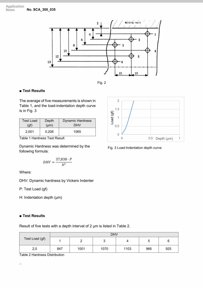
Fig. 2
■ Test Results The average of five measurements is shown in Table 1, and the load-indentation depth curve is in Fig. 3
Test Load (gf)
Depth (µm)
Dynamic Hardness DHV
2,001 0,206 1065
Table 1 Hardness Test Result
Dynamic Hardness was determined by the following formula:
𝐷𝐷𝐷𝐷𝐷𝐷𝐷𝐷𝐷𝐷𝐷𝐷 =37,838 ∙ 𝑃𝑃𝑃𝑃
ℎ2
Where:
DHV: Dynamic hardness by Vickers Indenter
P: Test Load (gf)
H: Indentation depth (µm)
Fig. 3 Load-Indentation depth curve
■ Test Results Result of five tests with a depth interval of 2 μm is listed in Table 2.
Test Load (gf) DHV
1 2 3 4 5 6
2,0 847 1001 1070 1103 966 925
Table 2 Hardness Distribution
..
0
0,5
1
1,5
2
0 0,5 1
Load
(gf)
Depth (µm)
No. SCA_300_035

■ Dynamic hardness was determined by the same formula as item 1) above. The Relation of depth and hardness is shown in Fig. 4.
Fig. 4
Fig. 4 indicates a tendency that hardness increases as depth increases, reaches the max. at mid depth of the plating layer, and decreases thereafter.
0
200
400
600
800
1000
1200
0 2 4 6 8 10 12 14
Achs
entit
el
Hardness (DHV)
No. SCA_300_035

Use Autograph to simply perform in-plane reverse loading tests on sheet metal. ■ In-Plane Reverse Loading Test It is a testing method, where a sheet metal is subjected to tensile compression tensile reverse loading and continuously measuring the stress-strain curve. It can be used to make highly accurate measurements of the Bauschinger effect or the strain dependence of the elastic modulus required for forming simulation. In-plane reverse loading is possible by gripping the specimen with a die (comb grips) movable in the testing axis direction to prevent a specimen from buckling.
■ Features Space-saving: Perform tests by attaching the jigs to Autograph. No specialized equipment required. Good operability: The jigs can be used sideways, making specimen setting easy. All operations from attachment of the jigs to testing can be performed by one person. Simple displacement measurement: Extension of the specimen can be measured using the strain gauge type extensometer. No need to attach a strain gauge to the specimen, making it possible to perform tests more efficiently. Simple operation: Any straightening pressure can be set easily using the hydraulic jack and hydraulic hand pump.
Material Testing System AG-X
Jigs for Measuring Bauschinger Effect No. SCA_300_045

■ External View of Jigs
Grip faces Upper Grip
Lower Grip SG Extensometer
Comb Grip
Hydraulic Jack
No. SCA_300_045

■ Example of Test Results True Stress-True Strain Curve Specimen: DP780 high strength steel, sheet thickness 1.4 mm
Specifications Applicable Testing Machine AG-100kN
Loading Capacity Tensile: 100 kN / Compression: 100 kN
Buckling Prevention Unit
Hydraulic Unit Hydraulic hand pump Straightening Pressure Max. 40 kN
Extensometer
Type Strain gauge type Gauge Length 50 mm
Measurement Range +50 %/-10 % Measurement Precision JIS B 7741 Class 1
Applicable Specimen
JIS 5
L200 mm x W40 mm Parallel section L60 mm x W40 mm 1–3 mm thick
JIS 5 Special Size (Wide specimen)
L200 mm x W45 mm Parallel section L60 mm x W35 mm 1–3 mm thick
Operational Temp. Range Room temperature The test data is used with kind permission from G-TEKT Corporation
No. SCA_300_045

曲げひずみ
曲げ応
力


ひずみ
応力


変位
試験
力


変位
試験
力


縦ひずみ
横ひずみ
応力


2. Aerospace Industry

Plastics
Stainless steel
Glass fiber
Titanium alloy
Ceramics
Natural andsynthetic rubber
Aluminum alloy
Carbon fiber
2. Aerospace Industry
EVEN LIGHTER INNOVATIVE MATERIALS
Materials used in aircraft can be broadly categorized into metal, non-metal and composite materials. All are light but strong, offering excellent machinability and heat resistance, and have been developed to provide the properties required for aircraft.
Metals are the major materials used in aircraft structures, of which the majority are aluminum alloys. Titanium alloys and stainless steel are also used for parts around the afterburner and for components subjected to the jet exhaust.
Since plastics are light, easy to color-mold, transparent to electromagnetic waves and also good electrical and thermal insulators, they are widely used for window glass, interior material and so on.
Apart from applications in reinforcement of glass-fiber- reinforced resins, glass materials are inserted between the aircraft outer surface and interior lining as sound and thermal insulators.
Since synthetic rubber materials offer better resistance to weather, heat, oil and chemicals than natural rubber, they are widely used in gaskets, packing, hoses, duct couplings and waterproof sheets. Natural rubber is commonly used in aircraft tires due to superior rubber elasticity, tear strength and abrasive resistance.

2. Aerospace Industry
C225-E032 Ultrasonic fatigue testing system with an average stress loading mechanism
SCA_300_001 Very high cycle fatigue (VHCF) assessment of laser additive manufactured (LAM) AlSi12 alloy
No.ei254 Compression after impact testing of composite
No.ei255 Compression testing of composite materials
No.36 Evaluating the fatigue strength of GFRP materials
No.30 Evaluating the strength of carbon fiber reinforced plastics (CFRP)
No.39 Evaluation of open-hole CFRP
No.i247 DIC analysis material testing by strain distribution visualization
No.8 Flexural testing of CFRP boards
No.16 Tensile testing of carbon fiber
No.31 Materials testing using digital image correlation
No.37 Observing the failure of open-hole CFRP samples in tensile tests
No.38 Observing the fracture of unidirectional CFRP in static tensile testing
No.ei256A Open-hole compression testing of com- posite material
No.ei250 Shear test of composite material (V-notched beam)
No.ei251 Shear test of composite material (V-notched rail shear)
SCA_300_037 Compression-rupture test of carbon fibers with different tensile characteristics Shimadzu micro compression testing machine MCT
SCA_300_059 Observation of fracture in CFRP tensile test E001HPV
C225-E032 Ultrasonic fatigue testing system with an average stress loading mechanism
No.i244 Tensile test for metallic materials using strain rate control and stress rate control
SCA_300_035 A hardness measurement of surface treatment layer on a steel sample using Shimadzu dynamic ultra micro hardness tester, model DUH
No.2 Flexural test of plastic ISO178
No.3 Tensile tests of plastic materials at low ISO527 1
No.4 Tensile test of rubber dumb bell specimens ISO37
No.5 Tear test of crescent shaped ISO34 1
No.6 Tear tests of angle shaped rubber specimens ISO34 1
No.7 Tensile tests of films ISO527 3
No.9 Measurements of modulus of elasticity and poisson’s ratio for films ISO527

C225-E032
Ultrasonic Fatigue Testing System Effective for Gigacycle Fatigue Tests
With fatigue tests of high-strength steels, it is evident that internal fracture (fish-eye fracture), which is caused by inclusions and other micro defects, occurs at 107 cycles or more, a value considered the conventional fatigue limit.An ultrasonic fatigue testing system is extremely effective when performing this sort of gigacycle fatigue test. (With a 100 Hz fatigue testing system, this would take 3 years, but if a 20 kHz ultrasonic fatigue testing system is used, testing can be completed in one week.)
Actual components are rarely used under conditions in which the average stress is zero. Despite this, the USF-2000A, a standard ultrasonic fatigue testing system, can only perform testing under zero average stress conditions.Using an ultrasonic fatigue testing system equipped with an average stress loading mechanism, gigacycle fatigue tests can be performed with average tensile stress loaded.
Ultrasonic Fatigue Testing System with an Average Stress Loading Mechanism
Stressdistribution
AG-X5kNAverage stress loading
High-rigidity booster
Horns
High-rigidity booster
5 kN load cellAverage stress measurement
Converter(Piezo actuator)
Strain GaugeSamples
DisplacementStress
System Appearance
For Gigacycle Fatigue Tests with Average Stress Loaded

© Shimadzu Corporation, 2016First Edition: August 2016
For Research Use Only. Not for use in diagnostic procedure. This publication may contain references to products that are not available in your country. Please contact us to check the availability of these products in your country.Company names, product/service names and logos used in this publication are trademarks and trade names of Shimadzu Corporation or its affiliates, whether or not they are used with trademark symbol “TM” or “®”. Third-party trademarks and trade names may be used in this publication to refer to either the entities or their products/services. Shimadzu disclaims any proprietary interest in trademarks and trade names other than its own.
The contents of this publication are provided to you “as is” without warranty of any kind, and are subject to change without notice. Shimadzu does not assume any responsibility or liability for any damage, whether direct or indirect, relating to the use of this publication.www.shimadzu.com/an/
Ultrasonic resonance systemPower supply, converter, booster (1 pair), horn (1 pair)
Personal computer(OS Windows 7) ADA/PIO interface board
SoftwareUltrasonic test control measurement software
Cooling systemAir dryer, air piping• A separate 140 L/min air source is required.
5 Strain meter unit (option)
6 AG-X plus Autograph 5 kN + 250 extension
7 Average stress loading mechanism
1
2
3
4
Main Speci�cations
1) Test Frequency: 20 kHz ± 500 Hz
• The recommended test range is 20 kHz ± 30 Hz.• The test frequency is determined by the resonance frequency of the sample.
2) Horn End Face Amplitude
Min. approx. ±10 μmMax. approx. ±50 μm
• The minimum and maximum amplitudes are the end face amplitude values at amplitude outputs of 20 % and 100 % respectively. Accordingly, the minimum and maximum amplitude values will change somewhat depending on the shape of the sample.
4) Average Stress
Max. 1.5 kN (tensile only)
3) Test Stress
Standard circular tapered sampleStress Min. 237 MPa Max. 1186 MPa• The test stress range can be changed by changing the sample shape.• The minimum and maximum values are calculated with the end face amplitude values of 10 μm and 50 μm respectively.• These are the values when the stress is within the elasticity range.
Standard Circular Tapered Sample
Surface of the Fatigued Fracture Originating from the Inclusion
Center hole can remain
Center holecan remain
Components

■ Introduction
Selective laser melting (SLM) is a laser additive manufacturing process where parts are additively manufactured using powder material with the aid of laser energy. Three-dimensional CAD model is provided as an input to the SLM machine, which scans the geometry after slicing the geometry into 2D layers. The laser energy selectively melts the powder particles at the desired location of the component to be manufactured. The unique manufacturing capability of SLM process makes it suitable for aerospace, automotive and biomedical applications. Several alloys like aluminum, titanium, steel and nickel-based alloys have been processed by SLM technique [1,2]. Although the fatigue strength diminishes for SLM processed materials in the “as-built” condition due to the process-inherent surface roughness, fatigue performance after post-processing is suitable for many applications in the aviation and medical industry [1].
Contrary to the previous assumption that the materials do not fail under fatigue if the applied stress is below the so-called fatigue limit; with the availability of the novel very high cycle fatigue (VHCF) testing techniques, it has been found that materials do fail under fatigue loading even when the stresses are below the conventional fatigue limit, suggesting the non-existence of such a limit [3,4]. Some alloys of both lattice types (bcc and fcc) show a change in crack initiation site from surface to subsurface in a region from HCF to VHCF [5].
■ Experimental methodology
The test samples of AlSi12 alloy were manufactured using a commercially available SLM system in an inert environment using argon gas. The details of the processing setup and parameters can be viewed in [1]. Quasi-static tensile tests were carried out according to ISO 6892-1:2009. Continuous load increase tests were carried out starting at low stress amplitude of 30 MPa. Stress amplitude was increased slowly at a rate of 10 MPa / 104 cycles. Load increase tests and constant amplitude testes were carried out at a frequency of 20 Hz. The results of process optimization, quasi-static properties, high cycle fatigue properties and the measurement methodology for characterization of process-induced defects are published in [2,6]. Two types of configurations are investigated in this study. For the batch I, no pre-heating of the base plate was applied; whereas samples of batch II were manufactured with a base plate heating (BPH) at 200 °C.
Very high cycle fatigue (VHCF) tests were carried out on an ultrasonic fatigue testing system at a frequency of 20 kHz. Fig. 1 shows the overview of the USF-2000 testing system by Shimadzu (http://www.shimadzu.de/usf-2000) and Fig. 2 explains the detailed principle of the test setup. Piezoelectric crystal is used in the actuator, which resonates at a fixed frequency of 20 kHz. In the ultrasonic fatigue testing system, vibrations are designed so that the longitudinal waves transmitted through the solid body resonate.
Shimadzu Ultrasonic Fatigue Testing System
Very High Cycle Fatigue (VHCF) Assessment of Laser Additive Manufactured (LAM) AlSi12 Alloy
No. SCA_300_001

Fig. 1: Overview of the ultrasonic fatigue testing system USF-2000 by Shimadzu
Fig. 2: Functional principle of specimen loading at ultrasonic fatigue testing system USF-2000
The specimen with geometry shown in Fig. 3 is clamped only at one threaded end on USF and is free at the bottom end. The specimen is designed in a way that maximum stress is experienced at the middle of the specimen and the maximum displacement occurs at the free end of the specimen. To eliminate the temperature effect due to high test frequency, the specimens were cooled with compressed air during tests and the tests were performed at a pulse-pause ratio of 50:50 i.e. the system was set to resonance for 200 ms and then stopped for the next 200 ms to cool down.
Fig. 3: Specimen geometry for ultrasonic fatigue tests
Experiments for determination of the fatigue strength at 109 cycles were performed according to stair-case method. If a specimen at ultrasonic frequency failed at less than 109 cycles, the stress amplitude is decreased by 5 MPa for the next experiment. If the specimen did not fail at 109 cycles, the stress amplitude was increased by 5 MPa in the subsequent test. Failure of the specimen is based on the change is resonance frequency. When the micro-crack leads to final fracture, the natural frequency of the system reduces than the operating frequency of the system and the test is terminated.
■ Results
Fig. 4 shows exemplary surface micrographs for the two investigated batches. The remnant porosity is viewed as only the gas porosity. A difference in the pore fraction of the samples without and with base plate heating is observed. In the samples with base plate heating, large size gas pores are absent which are very critical for fatigue performance. The reduction of large pores is attributed to the de-gassing in the manufacturing chamber due to pre-heating.
SCA_300_001

Fig. 4: Exemplary surface micrograph for sample without base plate heating (a); and with base plate heating (b)
Fig. 5 represents S-N curves for batches I and II in the region from high cycle fatigue (HCF) to very high cycle fatigue (VHCF). Experiments showed that the fatigue fracture occurs beyond high cycle fatigue region in both batches. The results of the experiments indicate that fatigue strength in very high cycle regime of samples manufactured with base plate heating is about 45% higher than fatigue strength of sample without base plate heating. Fatigue strength at one giga cycle for batches I and II is 60.5 ± 4.7 MPa and 88.7 ± 3.3 MPa, respectively. This increase in strength is attributed to elimination of the micro pores.
Fig. 5: S-N characterization for ultrasonic fatigue testing results
■ Outlook
New developments in testing machines enabled to go beyond the previously known limits of knowledge. This opens the door towards more intensive testing in the most realistic conditions. The new capabilities in testing machines shall provide researchers with powerful tools to further investigate the effect of processing parameters on the resulting functional performance in a wide range.
SCA_300_001

■ References
[1] Siddique, S.; Wycisk, E.; Frieling, G.; Emmelmann, C.; Walther, F.: Microstructural and mechanical properties of selective laser melted Al 4047. Applied Mechanics and Materials 752-753 (2015) 485–490.
[2] Siddique, S.; Imran, M.; Wycisk, E.; Emmelmann, C.; Walther, F.: Influence of process-induced microstructure and imperfections on mechanical properties of AlSi12 processed by selective laser melting. Journal of Materials Processing Technology 221 (2015) 205–213.
[3] Pyttel, B.; Schwerdt, D.; Berger, C.: Very high cycle fatigue – Is there a fatigue limit? International Journal of Fatigue 33 (2011) 49–58.
[4] Benedetti, M.; Fontanari, V., Bandini, M.: Very high cycle fatigue resistance of shot-peened high strength aluminium alloys. Experimental and Applied Mechanics 4 (2013) 203–211.
[5] Morrissey, R.J.; Nicholas, T.: Fatigue strength of Ti-6Al-4V at very long lives. International Journal of Fatigue 27 (2005) 1608–1612.
[6] Siddique, S.; Imran, M.; Rauer, M.; Kaloudis, M.; Wycisk, E.; Emmelmann, C.; Walther, F.: Computed tomography for characterization of fatigue performance of selective laser melted parts. Materials & Design 83 (2015) 661-669.
■ Contact Address
TU Dortmund University Materials Test Engineering (WPT) M.Sc. Shafaqat Siddique Baroper Str. 303 D-44227 Dortmund Tel.: +49 (0)231 755-8165 Fax: +49 (0)231 755-8029 E-Mail: [email protected] Web: www.wpt-info.de
TU Dortmund University Materials Test Engineering (WPT) Prof. Dr.-Ing. Frank Walther Baroper Str. 303 D-44227 Dortmund Tel.: +49 (0)231 755-8028 Fax: +49 (0)231 755-8029 E-Mail: [email protected] Web: www.wpt-info.de
SCA_300_001

ApplicationNews
No.i254
Material Testing System
Compression After Impact Testing of Composite
Material
LAAN-A-AG-E018
Introduction
Carbon fiber reinforced plastic (CFRP) has a higher specific strength and rigidity than metals, and is used in aeronaut ics and as t ronaut ics to improve fue l consumption by reducing weight. However, CFRP only exhibits these superior properties in the direction of its fibers, and is not as strong perpendicular to its fibers or between its laminate layers. When force is applied to a CFRP laminate board, there is a possibi l ity that delamination and matrix cracking will occur parallel to its fibers. Furthermore, CFRP is not particularly ductile, and is known to be susceptible to impacts. When a CFRP laminate board receives an impact load, it can result in internal matrix cracking and delamination that is not apparent on the material surface. There are many situations in which CFRP materials may sustain an impact load, such as if a tool being dropped onto a CFRP aircraft wing, or small stones hitting the a CFRP wing during landing. Consequently, tests are required for these scenarios. One of these tests is compression after impact (CAI) testing. CAI testing involves subjecting a specimen to a prescribed impact load, checking the state of damage to the specimen by a nondestruct ive method, and then performing compression testing of that specimen. This article describes CAI testing performed according to the ASTM D7137 (JIS K 7089) standard test method.
Measurements Taken Before Compression After Impact Testing
(1) Impact TestThe impact test involved dropping a 5 kg steel ball striker formed with a 16 mm diameter hemispherical point in the middle of the specimen. The specimen is fixed in place with four toggle clamps. The standard test method states that avoiding a second impact is preferred, so impact testing was performed with a mechanism that prevented second impacts. The impact energy recommended in the standard test method is 6.67 J per 1 mm of specimen thickness. For the purpose of comparison, the test was performed at four impact energies of 6.7, 5.0, 3.3, and 1.7 J per 1 mm thickness. Information on the specimen used is shown in Table 1. The test setup is shown in Fig. 1, and test conditions are shown in Table 2.
Dimensions [mm] : 100 × 150 × 4.56Lamination Method : [45/0/–45/90] ns
Material : T800, 2252S-21
Table 1 Specimen Information
Striker
SpecimenToggle clamp
Fig. 1 Impact Test Setup
Impact Energy : 30.5, 22.9, 15.2, 7.6 [J]No. of Tests : n = 4
Table 2 Impact Test Conditions
(2) Non-Destructive InspectionAfter the impact test, the delamination area and maximum delamination length that resulted inside the laminate board were measured by nondestructive analysis. An ultrasonic flaw detection device is normally used for the non-destructive inspection step of CAI testing. The standard test method states that if ultrasonic flaw detection shows damage is present across more than half the width of the specimen, edge effects cannot be ignored and lowering the impact energy should be considered. Fig. 2 shows the setup for ultrasonic flaw detection.
Fig. 2 Ultrasonic Flaw Detection

Region
No.
Percentage
Area
(%)
Absolute
Area
(mm2)
1 99.9988 3326.2400
No. Length (mm)
1 73.03
2 75.50
3 61.37
0
0
500
1000
1500
2000
2500
3000
3500
4000
4500
10 20
Impact Energy [J]
Dam
ag
e A
rea [
mm
2]
30 40
ApplicationNews
No.i254
Fig. 3 shows the specimen after an impact test with an impact energy of 30.5 J. Fig. 3 shows an indentation in the middle of the specimen, but does not show the area of damage caused by delamination. Fig. 4 shows the results of ultrasonic flaw detection at each impact energy. The white areas in Fig. 4 are regions of delamination. Brighter areas show greater delamination. Comparison with Fig. 3 shows that delamination also occurs in areas other than the indentation in the center of the spec imen, and the extent of interna l damage cannot be determined based on external damage. The re su l t s a l so show tha t the damage a rea increases as the impact energy increases.
Fig. 3 Specimen After Impact Test (30.5 J Impact Energy)
30.5 J 22.9 J
15.2 J 7.6 J
Fig. 4 Results of Ultrasonic Flaw Detection at Each
Impact Energy
The damage area and maximum damage length are calculated from the images obtained by ultrasonic f law detection. As an example, images used to calculate the damage area and maximum damage length after an impact energy of 30.5 J are shown in Fig. 5. Fig. 6 shows the relationship between damage area and impact energy, and F ig. 7 shows the relationship between maximum damage length and impact energy.
1
32
Fig. 5 Images of Damaged Area and Maximum Damage Length
Fig. 6 Relationship between Damage Area and Impact Energy
0
0
10
20
30
40
50
60
70
80
90
10 20
Impact Energy [J]Maxi
mu
m D
am
ag
e L
en
gth
[m
m]
30 40
Fig. 7 Relationship between Maximum Damage Length and
Impact Energy

Impact Energy [J]
Compression-After-
Impact Strength
[MPa]
Compressive Elastic
Modulus After
Impact [GPa]
30.5 162.9 57.2
22.9 203.3 56.4
15.2 246.4 56.0
7.6 308.6 56.3
ApplicationNews
No.i254
Measurement System for Compression After Impact Testing
Two strain gauges must be attached to the front and back of the specimen. A specimen with strain gauges attached is shown in Fig. 8. The specimen shown in Fig. 8 is compressed at up to 10 % its expected compressive strength following impact in a longi tud ina l d i rect ion, and the CAI test ing i s performed after confirming the difference between front and rear strain gauges is within 10 %. Test conditions are shown in Table 3. The test setup is shown in Fig. 9, and test equipment used is shown in Table 4.
Fig. 8 Specimen
Test Speed : 1.25 mm/minNo. of Tests : n = 4
Table 3 Test Conditions
Fig. 9 Test Setup
Testing Machine : AG-XplusLoad Cell : 250 kNTest Jig : Compression after impact test jig
Table 4 Experimental Equipment
Test Results
Examples of stress-strain curves at each impact energy are shown in Fig. 10. The compression-after-impact strength and mean compressive elastic modulus after impact are shown for each impact energy in Table 5. The standard test method states the compressive elastic modulus after impact should be calculated in the range of 0.1 % to 0.3 % strain. However, the breaking strain of one or more specimens was 0.3 % after the 30.5 J impact energy, and so for these specimens the elastic modulus was calculated from a linear region. Fig. 10 and Table 5 show the smaller the impact energy the larger the compression-after-impact strength. They also show the compressive elastic modulus after impact is almost constant regardless of impact energy.
0
0
50
100
150
200
250
300
350
0.1 0.2 0.3
Strain [%]
0.4 0.5 0.6
Str
ess
[M
Pa]
CFRP (30.5 J)
CFRP (22.9 J)
CFRP (15.2 J)
CFRP (7.6 J)
Fig. 10 Stress-Strain Curve
Table 5 Test Results (Mean)

ApplicationNews
No.
© Shimadzu Corporation, 2016
For Research Use Only. Not for use in diagnostic procedure.
This publication may contain references to products that are not available in your country. Please contact us to check the availability of these
products in your country.
The content of this publication shall not be reproduced, altered or sold for any commercial purpose without the written approval of Shimadzu.
Company names, product/service names and logos used in this publication are trademarks and trade names of Shimadzu Corporation or its
affiliates, whether or not they are used with trademark symbol “TM” or “®”. Third-party trademarks and trade names may be used in this
publication to refer to either the entities or their products/services. Shimadzu disclaims any proprietary interest in trademarks and trade names
other than its own.
The information contained herein is provided to you "as is" without warranty of any kind including without limitation warranties as to its
accuracy or completeness. Shimadzu does not assume any responsibility or liability for any damage, whether direct or indirect, relating to the
use of this publication. This publication is based upon the information available to Shimadzu on or before the date of publication, and subject
to change without notice.
www.shimadzu.com/an/
i254
First Edition: Aug. 2016
The re l a t i on sh ip be tween damage a rea and compression-after-impact strength is shown in Fig. 11, and the relationship between maximum damage length and compressive elastic modulus after impact is shown in Fig. 12. Fig. 11 and Fig. 12 show the smaller the damage area or maximum damage length, the larger the compression-after-impact strength. As a reference, the compressive strength of a specimen tested without applying any impact energy was 388 MPa.
0 1000 2000 3000
Damage Area [mm2]
Co
mp
ress
ion
-Aft
er-
Imp
act
Str
en
gth
[M
Pa]
4000 5000
0
50
100
150
200
250
300
350
400
450
Fig. 11 Relationship between Damage Area and Compression-
After-Impact Strength
0
0
50
100
150
200
250
300
350
400
450
20 40 60
Maximum Damage Length [mm]
Co
mp
ress
ion
-Aft
er-
Imp
act
Str
en
gth
[M
Pa]
80 100
Fig. 12 Relationship between Maximum Damage Length and
Compression-After-Impact Strength
Conclusion
CAI testing was performed on specimens at four different impact energies. As shown by the results, the la rger the impact energy the smal le r the compression-after-impact strength. Also, even a small amount of impact energy (in this experiment, an impact energy of 7.6 J amounted to 5 kg dropped from 0.15 m) reduced the compression-after-impact strength compared to the undamaged compressive s t rength , showing the impor tance of tes t ing scenarios for impact loading. Shimadzu's testing system was used successfully to perform CAI testing according to ASTM D7137 (JIS K 7089), and can be used for evaluation of CFRP materials.

ApplicationNews
No.i255
Material Testing System
Compression Test of Composite Material
LAAN-A-AG-E019
Introduction
Even among composite materials, carbon f iber reinforced plastic (CFRP) has a particularly high specific strength, and is used in aeroplanes and some transport aircraft to improve fuel consumption by reducing weight. Compressive strength is an extremely important parameter in the design of composite materials that is always tested. However, due to the difficulty of testing compressive strength there is a variety of test methods. A major compression test method is the combined loading compression (CLC) method found in ASTM D6641. The CLC method can be performed with a simple jig structure, untabbed strip specimens, and can be used to simultaneously evaluate strength and measure elastic modulus. We performed compression testing of CFRP according to ASTM D6641.
Measurement System
A CFRP specimen of T800S/3900 was used. Other information on the specimen is shown in Table 1. The test equipment used is shown in Table 2. Based on the CLC method in ASTM D6641, the specimen was attached to the jig shown in Fig. 1 and compressed using compression plate. Fig. 2 shows a photograph of the specimen. As shown in Fig. 2, a strain gauge was attached on the front and rear in the middle of the specimen. Outputs from the front and rear strain gauges confirmed that the specimen was aligned straight in the jig during specimen attachment. The specimen was attached using a torque wrench to fasten it in place uniformly. The test was performed with the test speed set to 1.3 mm/min.
Length : 140 mmWidth : 13 mmThickness : 3 mmLamination Method : [90/0] 4S
Table 1 Specimen Information
Testing Machine : AG-XplusLoad Cell : 50 kNTest Jig : CLC test fixture
Table 2 Experimental Equipment
Fig. 1 Test Fixture
Fig. 2 Specimen
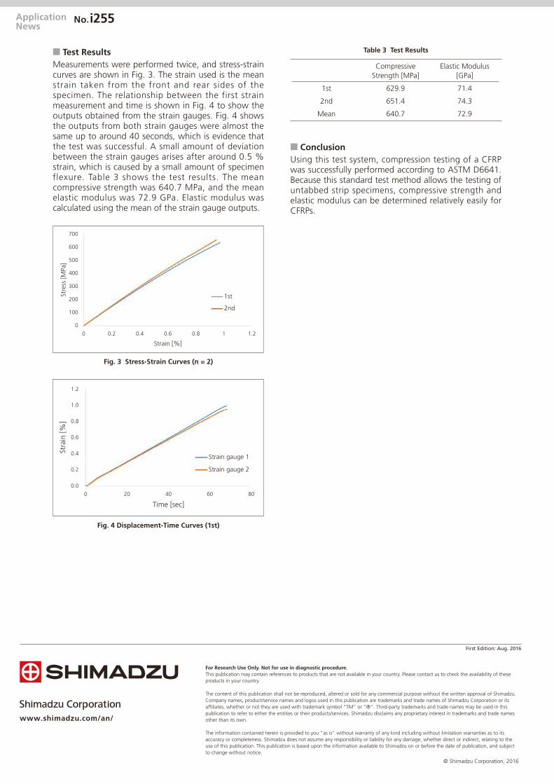
Compressive
Strength [MPa]
Elastic Modulus
[GPa]
1st 629.9 71.4
2nd 651.4 74.3
Mean 640.7 72.9
ApplicationNews
No.
© Shimadzu Corporation, 2016
For Research Use Only. Not for use in diagnostic procedure.
This publication may contain references to products that are not available in your country. Please contact us to check the availability of these
products in your country.
The content of this publication shall not be reproduced, altered or sold for any commercial purpose without the written approval of Shimadzu.
Company names, product/service names and logos used in this publication are trademarks and trade names of Shimadzu Corporation or its
affiliates, whether or not they are used with trademark symbol “TM” or “®”. Third-party trademarks and trade names may be used in this
publication to refer to either the entities or their products/services. Shimadzu disclaims any proprietary interest in trademarks and trade names
other than its own.
The information contained herein is provided to you "as is" without warranty of any kind including without limitation warranties as to its
accuracy or completeness. Shimadzu does not assume any responsibility or liability for any damage, whether direct or indirect, relating to the
use of this publication. This publication is based upon the information available to Shimadzu on or before the date of publication, and subject
to change without notice.
www.shimadzu.com/an/
i255
First Edition: Aug. 2016
Test Results
Measurements were performed twice, and stress-strain curves are shown in Fig. 3. The strain used is the mean strain taken from the front and rear sides of the specimen. The relationship between the first strain measurement and time is shown in Fig. 4 to show the outputs obtained from the strain gauges. Fig. 4 shows the outputs from both strain gauges were almost the same up to around 40 seconds, which is evidence that the test was successful. A small amount of deviation between the strain gauges arises after around 0.5 % strain, which is caused by a small amount of specimen flexure. Table 3 shows the test results. The mean compressive strength was 640.7 MPa, and the mean elastic modulus was 72.9 GPa. Elastic modulus was calculated using the mean of the strain gauge outputs.
1st
2nd
0
0
100
200
300
400
500
600
700
0.2 0.4 0.6
Strain [%]
Str
ess
[M
Pa]
0.8 1 1.2
Fig. 3 Stress-Strain Curves (n = 2)
0.0
0.2
0.4
0.6
0.8
1.0
1.2
Str
ain
[%
]
0 20 40 60 80
Time [sec]
Strain gauge 1
Strain gauge 2
Fig. 4 Displacement-Time Curves (1st)
Table 3 Test Results
Conclusion
Using this test system, compression testing of a CFRP was successfully performed according to ASTM D6641. Because this standard test method allows the testing of untabbed strip specimens, compressive strength and elastic modulus can be determined relatively easily for CFRPs.

■
■
°
°
■
LAAN-J-SB002

■
www.shimadzu.com/an/
Shimadzu Corporation

■
■
■
× × × ×
×

×
υ εευ ε ε
■

LAANJAG0035
Material Testing & Inspection
Autograph Precision Universal Testing Machine
Evaluation of OpenHole CFRP— Static Tensile Testing, Fracture Observation,
and Internal Structure Observation —
IntroductionRecently, lightweight alternatives to conventional metal
materials are being used as structural members where mechanical reliability is required. The main reason for this trend is that lighter products reduce transport weights, which reduces fuel consumption and carbon dioxide emissions during product transport. Fiber reinforced composite materials such as carbon fiber reinforced plastics (CFRP), which consist of a resin strengthened with carbon fibers, are extremely strong and light. Because of this, they are currently a material widely used in aircraft, and are expected to be used increasingly in various types of products, including automobiles, in order to make them lighter. For the development of fiber reinforced composite materials, not just a simple evaluation of their mechanical strength, but also the observation of failure events is important. In addition, from the perspective of quality management, the necessity for evaluation of internal structure of these materials, such as the oriented state of fibers and the presence of cracks, has increased.
In this article, we describe how we use a precision universal testing machine (Autograph AG250kNXplus) and highspeed video camera (HyperVision HPVX) (Fig. 1) to evaluate the static fracture behavior of a CFRP based on a test force attenuation graph and images of material failure. We also describe our subsequent examination of the state of the specimens internally using an Xray CT system (inspeXioSMX100CT) to investigate the state of fracture inside the specimen. Information on specimens is shown in Table 1. Specimens have a hole machined into their center that is 6 mm in diameter. Fracture is known to propagate easily through composite materials from the initial damage point, and when a crack or hole is present their strength is reduced markedly. Therefore, evaluation of the strength of openhole specimens is extremely important from the perspective of the safe application of CFRP materials in aircraft, etc.
Note: The CFRP laminate board used in the actual test was created by laying up prepreg material with fibers oriented in a single direction. The [+45/0/45/+90]2s shown as the laminate structure in Table 1 refers to the laying up of 16 layers of material with fibers oriented at +45, 0, 45, and +90 in two layer sets.
Table 1: Test Specimen Information
Laminate StructureDimensionsL (mm) × W (mm) ×T (mm), hole diameter (mm)
[+45/0/45/+90]2s 150 ×36×2.9, Φ6
Fig.1: Testing Apparatus
In this test, the change in load that occurs during specimen fracture was used as the signal for the HPVX highspeed video camera to capture images. Specifically, the AGXplus precision universal testing machine was configured to create a signal when the test force on the specimen reaches half the maximum test force (referred to as Maximum test force in Fig. 3), with this signal being sent to the highspeed video camera. Static tensile testing and fracture observation were performed according to the conditions shown in Table 2. A test forcedisplacement plot for the openhole quasiisotropic CFRP(OHCFRP) is shown in Fig. 2(a). A test forcetime plot during the occurrence of material fracture is also shown in Fig. 2(b).
Static Tensile Testing (Ultra High Speed Sampling)
HyperVision HPVX highspeed video camera
Autograph AGXplus
Light source
Trigger Signal

Fig. 3: Observations of OHCFRP Fracture
Testing Machine AGXplus
Load Cell Capacity 250 kN
Jig
Upper: 250 kN nonshift wedge type grips (with trapezoidal file teeth on grip faces for composite materials)Lower: 250 kN highspeed triggercapable grips
Grip Space 100 mm
Loading Speed 1 mm/min
Test Temperature Room temperature
Software TRAPEZIUM X (Single)
Fracture Observation HPVX highspeed video camera (recording speed 600 kfps)
DIC Analysis StrainMaster (LaVision GmbH.)
Table 2: Test Conditions
Note: fps stands for frames per second. This refers to the number of frames that can be captured in 1 second.
0 20 40 60 80 100 120 140 160 180 2000
20000
40000
60000
80000
Forc
e (
N)
Time (μs)
Fig. 2 (a) Test ForceDisplacement Curve, and (b) Test ForceTime Curve (in Region of Maximum Test Force)
Maximum test force
Forc
e (N
)
Time (s)
Change in test force can be measured in detail during fracture occurrence
The interval between data points on the test force plot is approximately 3.3 s.Fo
rce
(N)
Time (s)
(a)
(b)
Fig. 2(a) can be interpreted to show the specimen fractured at the moment it reached the maximum test force, at which point the load on the specimen was suddenly released. This testing system can be used to perform highspeed sampling to measure in detail the change in test force in the region of maximum test force. The time interval between data points on the test force plot in Fig. 2(b) is 3.3 s.
Images (1) through (8) in Fig. 3 capture the behavior of the specimen during fracture around the circular hole. Image (1) shows the moment cracks occur in a surface +45 layer. In this image, the tensile load being applied is deforming the circular hole, where hole diameter in the direction of the load is approximately 1.4 times that perpendicular to the load. In image (2), the cracks that occurred around the circular hole are propagating along the surface +45 layer. In images (3) through (6), a substantial change can be observed in the external appearance of the specimen near the end of the crack propagating to the bottom right from the circular hole. This suggests not only the surface layer, but internal layers are also fracturing. Based on the images of the same area and the state of the internal layers that can be slightly observed from the edges of the circular hole in images (7) and (8), the internal fracture has quickly propagated in the 18 s period between images (3) and (8).
Fracture Observation (High Speed Imaging)

Fig. 4: Observation of OHCFRP Fracture (DIC Analysis)
Images (1) through (8) of Fig. 4 show the results of performing Digital image correlation (DIC) analysis on the fracture observation images of Fig. 3. Black signifies areas of the surface layer of the specimen under little strain, and red signifies areas under substantial strain. Looking at images (1) through (4), we can see that strain around the circular hole is focused diagonally toward the topleft (45) and toward the bottomleft (+45) from the circular hole. Images (5) through (8) show the focusing of strain diagonally toward the bottomright (45) and toward the topright (+45) from the circular hole in areas where it was not obvious in images (1) through (4). This shows an event is occurring in the surface layer of the specimen that is similar to the process of fracture often seen during tensile testing of ductile metal materials, which is crack propagation in the direction of maximum shearing stress.
Next, internal observations were performed around the circular hole using a micro focus Xray CT system to check the state of internal damage to the specimen. The SMX100CT micro focus Xray CT system (Fig. 5) is capable of capturing CT images at high magnification. The system rotates a specimen between an Xray generator and an Xray detector, uses a computer to calculate fluoroscopic images obtained from all 360 of rotation, then reconstructs a tomographic view of the specimen (Fig. 6). This system was used to perform a CT scan of the fracture area of the OHCFRP after the static tensile testing and fracture observation performed as described in the previous section, so that the cracks that occurred inside can be observed.
Fig. 5: Shimadzu inspeXio SMX100CT Micro Focus XRay CT System
Fig. 6: Illustrated Example of XRay CT System Operation
Fig. 7: Specimen After Static Tensile Testing (Specimen Used for CT Scan)
Fig. 8: Fracture Area 3D Image No. 1
Internal Structure Observation (CT)

Crosssectional images of the specimen are shown as a 3D image in the 16 layers shown in Fig. 9, we can see that most cracks in the matrix occur in the +45 layer inside the specimen, indicated by the number (1) and (3). (shown in Fig. 10 (a) and Fig. 10 (b), respectively). In this layer, the carbon fibers are all aligned together in a +45 orientation, and the multiple matrix cracks occurring in this layer are probably due to the shearing force caused in this layer by tensile loading, together with deformation of adjacent layers in the direction of the loading. For comparison, a 3D image of the 45 layer inside the specimen (Fig. 9 (2)) is shown in Fig. 10 (b). As is clear from the image, the matrix cracks that occurred in the +45 layer have not occurred in the 45 layer. This difference in fracture state has probably arisen due to different shearing forces and load directions occurring in each layer. Such detailed observation of fracture surfaces associated with multiple matrix cracks was difficult by conventional methods, since to observe fracture surfaces the specimen was processed such as by cutting and embedding in resin, which changed the characteristics of the specimen. However, by using the highresolution Xray CT system as described in this article, there is little Xray absorption difference between air and specimen, and it is possible to observe the state of complex internal damage, even for OHCFRP in which microscopic damage is normally difficult to observe by Xray.
Fig. 9: CT CrossSectional Images of the Fracture Area
Fig. 10: Fracture Area 3D Image No. 2
We would like to extend our sincere gratitude to the Japan Aerospace Exploration Agency (JAXA) for their cooperation in the execution of this experiment.
Acknowledgment
Note: The analytical and measuring instruments described may not be sold in your country or region.

ApplicationNews
No.i247
Material Testing System
Material Testing by Strain Distribution Visualization – DIC Analysis –
LAAN-A-AG-E012
Strain distribution in samples is an increasingly important component of material testing.As background to this trend, CAE (Computer Aided Engineering) is an analytical technology that is becoming widely used in the fields of science and industry due to the cost savings achieved through the reduced use of costly prototyping which is now being replaced by computerized product design simulation. A typical requirement is to conduct mechanical testing analysis of the region of a product in which strain is likely to occur, and to elucidate the correlation between the simulated analysis results and the strain distribution obtained in actual mechanical testing.DIC (Digital Image Correlation) analysis is a technique used to compare the random patterns on the surface of a test sample before and after deformation to determine the degree of deformation of the sample. The advantages of this technique include the ability to measure displacement and strain distribution from a digital image without having to bring a sensor into contact with a test sample, and without requiring a complicated optical system. For these reasons, application development for DIC analysis is expanding into a wide range of fields in which measurement using existing technologies*1 has been difficult.
n Introduction
Fig. 1 shows the testing apparatus and software used in the high-speed tensile testing of CFRP. The test conditions are shown in Table 1, and information regarding the test specimens is shown in Table 2. For this experiment, special-shaped grips for composite materials were mounted to the HITS-T10 high-speed tensile testing machine, and the test specimen was affixed to the grips.A high-speed HPV-2A video camera was mounted in front of the testing gap between the grips to collect video data of the specimen breaking, and the signal to start camera filming was a displacement signal from the high-speed tensile testing machine. The acquired video data was loaded into the StrainMaster (LaVision GmbH) DIC analysis software, and the strain distribution that occurred in the sample was analyzed.
n Test Conditions
Fig. 1 Testing Apparatus
Here we introduce examples of DIC analysis of CFRP (Carbon Fiber Reinforced Plastic) and ABS resin high-speed tensile impact testing.
*1: Up to now, material strain distribution measurement has been conducted using various methods, including the direct attachment of large numbers of strain gauges to the test material. However, this method is not applicable for micro-sized samples to which strain gauges either cannot be attached, or attachment is difficult and complicated. These disadvantages also include the difficulty in measuring certain types of substances, such as films, that are easily affected by contact-type sensors.
StrainMaster (LaVision GmbH)
HPV-2A High Speed Video Camera
Test Grips and Test SpecimenHITS-T10 High Speed Tensile Testing Machine

ApplicationNews
No.
For Research Use Only. Not for use in diagnostic procedures.The content of this publication shall not be reproduced, altered or sold for any commercial purpose without the written approval of Shimadzu. The information contained herein is provided to you "as is" without warranty of any kind including without limitation warranties as to its accuracy or completeness. Shimadzu does not assume any responsibility or liability for any damage, whether direct or indirect, relating to the use of this publication. This publication is based upon the information available to Shimadzu on or before the date of publication, and subject to change without notice.
© Shimadzu Corporation, 2012www.shimadzu.com/an/
i247
First Edition: Dce, 2012
Table 1 Test Conditions
Table 2 Samples
InstrumentationHITS-T10 high-speed tensile testing machineHPV-2A high-speed video camera
Test Force Measurement 10 kN load cellTest Speed 10 m/sGrips Special grips for composite materialsSampling 250 kHzImaging Speed 500 kfpsLight Source Strobe
DIC AnalysisStrainMaster (LaVision GmbH)With cooperation of MARUBUN CORPORATION
Samples(dimensions)
CFRP-OH*2 Laminate method [0/90]2s*3
(Hole diameter ф1 mm, W8 × t0.4 reed-shaped)ABS resin (ASTM L-shaped test specimenTotal length 60 mm, Parallel part 3.2 (W) × 3.2 (T) mm)
MarkingCFRP-OH*2 : White random patternABS resin : Black random pattern
*2: OH: Abbreviation for Open Hole. Refers to a hole that is opened in a CFRP plate.
*3: The CFRP laminate used in this experiment is prepared by laminating prepreg fibers oriented in one direction. The [0/90]2s
specified for "Laminate method" in the table represents two sets of prepreg layers stacked in the 0 ° direction and 90 ° direction.
n Test Results
In this test, the HITS-T10 high speed tensile testing machine and HPV-2A high speed video camera were synchronized to take video at the instant the sample fractured. The sample was prepared prior to the test by spraying paint onto its surface in a random pattern, and the strain distribution on the surface of the test specimen was visualized by DIC analysis based on the amount of shift of the random pattern.
(1) (2) (3)
(5)(4) (6)
Fig. 2 Results of DIC Analysis of CFRP-OH Specimen
Fig. 3 Results of DIC Analysis of ABS Resin Specimen
(1) (2) (3) (4) (5)
In Fig. 3, localized strain occurs from the edge of the parallel region of the test specimen, and as time progresses, localized strain is noticeable at the upper and lower edge of the parallel region. Thus, by combining a high-speed tensile testing machine with a high-speed video camera, in addition to DIC analysis software, it has become possible to visualize the distribution of strain generated in a test specimen.
Fig. 2 and Fig. 3 show the DIC analysis results obtained in tensile testing of CFRP-OH and ABS resin test specimens, respectively. The images were extracted in the order of a typical time course analysis (image order corresponding to the numbers shown in images), from the start of the tensile test to the point that the specimen breaks. The appearance of coloring in the images corresponds to the strain distribution in the specimen. The amount of strain that occurs in the specimen corresponds to the degree of color warmth, with areas of darker color (such as blue-black) indicating low strain, and areas of brighter color (such as red-orange) indicating a greater degree of strain. It is clear that in Fig. 2, as the load is applied to the test specimen, the strain increases in the vicinity of the open hole. Because the test specimen is a [0/90]2s laminate material, it is believed that the fibers are aligned in the tensile direction in the test specimen surface layer which was subjected to random marking.

8 Flexural Testing of CFRP Boards
LAAN-J-AG-E008
Material Testing & Inspection
Standard No. JIS K 7074: 1988
Introduction
Measurement Results
Measurements and Jigs
Carbon fiber reinforced plastic (CFRP) is a composite material with excellent relative strength. This plastic was quickly adopted in the aviation and space sectors, and has contributed significantly to reducing fuselage weight. Initially, this plastic was only used for partial replacement of metal materials. In the latest aircraft, however, composite materials, primarily CFRP, represent 50 % of the fuselage weight. Improved productivity and reduced costs are expected due to subsequent technical developments, and it can be expected that this plastic will also become popular as a main material in automobile frames. In this Data Sheet, a CFRP clothwas subjected to a flexural testing using a precision universal tester in order to evaluate the strength of the material.
F. Yano
Fig. 1: Flexural Testing Schematic
支持台
Indenter
Test Specimen
D
R5
R2
80
In flexural testing specified in JIS K7074, a loading edge radius of 5 mm, and a support radius of 2 mm are specified. The specimen standard dimensions are specified as follows:
Length = 100 mm 1 mmWidth = 15 mm 0.2 mmThickness = 2 mm 0.4 mm
For tests performed using a specimen with the standard dimensions, the span between supports (L) will be 80 mm 0.2 mm. When TRAPEZIUM software is used, the flexural stress can be automatically calculated and plotted in a graph from the test force and the specimen dimensions. The flexural strength and other characteristic values can also be obtained from a few simple operations.
Fig. 2: Flexural Testing Status Fig. 3: Stress – Displacement Curve
Stre
ss (N
/mm
2)
Displacement (%)
Table 2: Test Results (Average)Load at Fracture (N) Bending Strength (%)
485 95
Table 1: Test ConditionsItem Set Value
Cell Capacity 5 kNLoad Speed 5 mm/min
Autograph Precision Universal Tester

8
First Edition: February 2013
© Shimadzu Corporation, 2013www.shimadzu.com/an/
Shimadzu Corporation
CFRP Flexural Testing System
Tester: AG-XplusLoad Cell: 5 kNTest Jig: Three-point bending test jig for plasticsSoftware: TRAPEZIUM X (Single)
AGS-X Table-Top Precision Universal Tester
A high-precision load cell is adopted. (The high-precision type is class 0.5; the standard-precision type is class 1.)Accuracy is guaranteed over a wide range, from 1/1000 to 1/1 of the load cell capacity. This supports highly reliable test evaluations.
Crosshead speed rangeTests can be performed over a wide range from 0.0005 mm/min to 1,500 mm/min.
High-speed samplingUltrafast sampling, as fast as 0.2 msec. Sudden changes in test force, such as when brittle materials fracture, can be assessed.
TRAPEZIUMX operational softwareDesigned for intuitive operation, this software offers excellent convenience and user friendliness.
Smart controllerReal-time test force and position data is readily confirmed, and the manual dial can be used for fine adjustments to jig positioning.
Optional Test DevicesA variety of tests can be conducted by switching between an abundance of jigs in the lineup.
Features
AG-Xplus Table-Top Precision Universal Tester

16
LAAN-J-AG0016
Material Testing & Inspection
Autograph Precision Universal Tester
Measurement Results
In this test, the test sample is fixed to a test specimen mounting board made from a paper, metal, or resin sheet as shown in Fig. 1, installed in the grips, and the tensile test is performed. The standard describes in detail the shape of the mounting board, the type of adhesive used to fix the carbon fiber to the mounting board, and the procedure for installing the carbon fiber (for details refer to the standard). The tests were carried out using clip type grips whose grip force could be adjusted in accordance with the strength of the sample.
Measurements and Jigs
Carbon fiber is an important industrial material, being essential in carbon fiber reinforced plastics (CFRP), having a specific gravity one-fourth that of normal steels, and a specific strength of 7 times. In this Application Data Sheet, examples of tensile testing of single carbon fibers based on the ISO standard are introduced.
T. Murakami
Introduction
Standard No. ISO11566: 1996 (JIS R 7606: 2000)
Fig. 1 Test Sample and Mounting Board (frame)
Single carbon fiber
Position for cutting mounting board Adhesive
Sample Diameter Tensile Strength Elongation at Break
Carbon fiber 6 m 7.1 GPa 2.84 %
Table 2 Test Results (average)
Fig. 2 Test Status
Tensile Testing of Carbon Fiber
Fig. 3 Test Results
Stre
ss (G
Pa)
Strain (%)
Table 1 Test Conditions
Item Set Value Test speed 1 mm/minDistance between grips 25 mm

16
First Edition: February 2013
© Shimadzu Corporation, 2013www.shimadzu.com/an/
Shimadzu Corporation
High Accuracy Displacement MeasurementA high accuracy (0.2 m) linear sensor has been adopted for measurement of displacement in the load direction. In addition, the backlash-free structure makes it possible to carry out testing with good accuracy.Displacement in the load direction of the test sample can be set accurately to a displacement display resolution of 0.02 m and a control resolution of 0.005 m.
Measurement of Micro Test ForcesA wide range of load cells from 0.5 N to 2 kN assures a precision of 1 % for measurements of testing forces of 2 mN at minimum.
Positioning Very Small Test SamplesUsing an X-Y stage (optional), very small test samples can be easily positioned.The position of the test samples can be observed using a stereo microscope.
High Rigidity FrameA high rigidity frame (45 kN/mm minimum) has been adopted to enable measurement of minute displacements.
Optional Test DevicesA variety of tests can be accommodated by switching between an abundance of jigs in the lineup.
Features
Shimadzu Autograph MST-1 Micro Strength Evaluation Testing Machine
Carbon Fiber Tensile Test System
Tester: MST-I Type HRLoad Cell: 1 N Test Jig: 1 N clip type grips (rubber-coated teeth), X-Y stage Software: TRAPEZIUM X (Single)

■
■
≈ σ τ στ


■

■
■
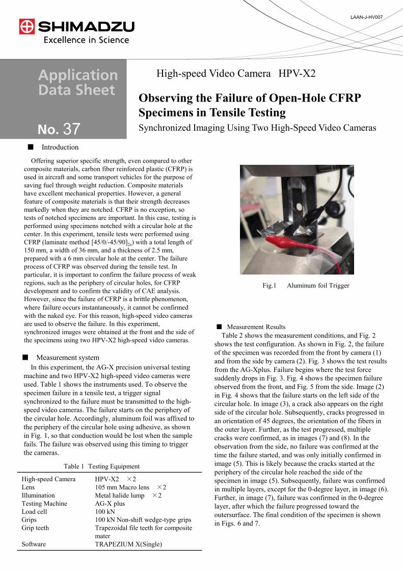
■
■
× × ×
■

① ②
① ② ③ ④
⑤ ⑥ ⑦ ⑧
⑨ ⑩ ⑪ ⑫

① ② ③ ④
⑤ ⑥ ⑦ ⑧
⑨ ⑩ ⑪ ⑫

■
www.shimadzu.com/an/
Shimadzu Corporation
First Edition: July, 2015

Results

(1) (2) (3) (4)
(5) (6) (7) (8)
(9) (10) (11) (12)
www.shimadzu.com/an/
Shimadzu Corporation
First Edition: July, 2015

Specimen NameOpen-Hole Compressive
Strength
1st 278.2 MPa
2nd 273.0 MPa
Mean 275.6 MPa
ApplicationNews
No.i256
Material Testing System
Open-Hole Compression Test of Composite Material
LAAN-A-AG-E020
Introduction
Carbon fiber reinforced plastic (CFRP) has gained attention due to their strength and low weight, and have quickly been adopted for use in aeronautics and astronautics. CFRP has excellent strength characteristics in terms of specific strength and high rigidity, but lose much of their strength when a cutout is made. Consequently, composite materials used in aeroplanes must be evaluated by tests that use specimens with a hole cut out of their center. We performed open-hole compression testing of a CFRP according to ASTM D6484.
Measurement System
The CFRP spec imen used was T800S/3900. As shown in Fig. 1, a hole was created in the middle of the spec imen. ASTM D6484 descr ibes tes t methods in both SI and Imperial units, where the dimensions of the j igs and specimens differ in each. We performed testing with Imperial units. Specimen information is shown in Table 1.ASTM D6484 inc ludes two load ing methods , which are described as Method A and Method B. In Method A, the specimen and test f ixture are clamped in a gripping device, and the specimen is compressed by shear force applied by the fixture and gripping device. In Method B, compression plate is present at the ends of the specimen and fixture, and are used to compress the specimen. Method B was used, as shown in Fig. 2. Table 2 shows a l ist of the equipment used and Table 3 shows the test conditions used.
Length : 30 mmWidth : 38.1 mmThickness : 3.1 mmLamination Method : [45/0/–45/92] 2S
Table 1 Specimen Information
Fig. 1 Specimen
Fig. 2 Test Setup
Testing Machine : AG-XplusLoad Cell : 50 kNTest Fixture : Open-Hole Compression Test Fixture
Table 2 Experimental Equipment
Test Speed : 2 mm/min
Table 3 Test Conditions
ResultsMeasurements were performed twice. Test results are shown in Table 4 and stress-displacement curves are shown in Fig. 3. As shown in Table 4, the mean open-hole compressive strength was 275.6 MPa.
Table 4 Test Results

0
0
20
40
6080
100
120
140
160
180
200
220240
260
280
300
0.2 0.4 0.6 0.8 1 1.2
Displacement (mm)
Str
ess
(N
/mm
2)
1.4 1.6 1.8 2 2.2 2.5
ApplicationNews
No.
© Shimadzu Corporation, 2016
For Research Use Only. Not for use in diagnostic procedure.
This publication may contain references to products that are not available in your country. Please contact us to check the availability of these
products in your country.
The content of this publication shall not be reproduced, altered or sold for any commercial purpose without the written approval of Shimadzu.
Company names, product/service names and logos used in this publication are trademarks and trade names of Shimadzu Corporation or its
affiliates, whether or not they are used with trademark symbol “TM” or “®”. Third-party trademarks and trade names may be used in this
publication to refer to either the entities or their products/services. Shimadzu disclaims any proprietary interest in trademarks and trade names
other than its own.
The information contained herein is provided to you "as is" without warranty of any kind including without limitation warranties as to its
accuracy or completeness. Shimadzu does not assume any responsibility or liability for any damage, whether direct or indirect, relating to the
use of this publication. This publication is based upon the information available to Shimadzu on or before the date of publication, and subject
to change without notice.
www.shimadzu.com/an/
i256
First Edition: Aug. 2016
Fig. 3 Stress-Displacement Curves
Results (DIC Analysis)
Using the TRViewX non-contact extensometer allows for images and video of the specimen to be collected synchronized with test result col lect ion. Also, applying a random pattern of paint to the observed specimen surface allows the images or video to be used to determine the strain distribution on the observed specimen surface during the test by DIC analysis1). Open-hole compression testing and DIC ana lys i s were per formed us ing the spec imen described in Table 5. Fig. 4 shows a photograph of the open-hole compression test system with a non-c o n t a c t e x t e n s o m e t e r. F i g . 5 s h o w s s t r a i n distributions around the open hole in the specimen that were obtained by DIC analysis. Fig. 5 shows that strain accumulates at the vertical sides of the open hole (regions (1) and (3)), strain appears along the axis of compression from those points, and the final break occurs at the vert ica l s ides of the hole. Meanwhile, almost no strain appears in the central part of the hole (region (2)) throughout the test. This strain distribution probably occurred due to a 0˚ fiber orientation on the surface of the specimen.
Length : 30 mmWidth : 38 mmThickness : 1.6 mmLamination Method : [0/90] 2S
Table 5 Specimen Information (DIC)
1) DIC analysis is an analysis method that measures strain and showsthe strain distribution in a specimen based on movement of arandom pattern of paint applied to the observed specimen surfacebefore and during testing.
Fig. 4 Experimental Setup (DIC)
①②③
1 2 3
4 5 6
Fig. 5 DIC Analysis Results
Conclusion
Using this test system, open-hole compression testing of a CFRP was successfully performed according to ASTM D6484. Using a non-contact extensometer, we were also able to capture video (images) synchronized with the test force and crosshead displacement data obtained from the testing machine. Performing DIC analysis based on this video allowed an evaluation of the strain distribution on the observed specimen surface. This testing system will be extremely useful for the development of CFRPs and products that use CFRPs.
Edition: . 2016

ApplicationNews
No.i250
Material Testing System
Shear Test of Composite Material
(V-Notched Beam)
LAAN-A-AG-E015
Introduction
Carbon fiber reinforced plastic (CFRP) do not oxidize or rust and have a higher specific strength and stiffness than existing materials. Applications of CFRP are being investigated, with a focus on applications as industrial products that require strength and durability. Compared to exist ing homogeneous materials, composite materials like CFRP are anisotropic, and display complex failure behaviors as a result of tension, compression, bending, in-plane shear, out-of-plane shear, or a combination of these stresses arising from loading in the principal-axis direction. In recent years, use of CAE analysis in industry has become widespread since it can reduce numbers of prototypes and reduce the cost of new product development. Because values for each of the stress properties stated above are needed to i n c rea se p re c i s i on when p red i c t i ng p roduc t characteristics during product design, there is a strong demand for test methods able to evaluate pure failure behaviors in CFRP.This article describes an example of V-notched beam method (Iosipescu method, ASTM D5379) that is widely used as an in-plane shear test method for composite material specimens. The test method can apply load as a pure in-plane shear stress on the evaluation area (see Fig. 1) by using a specimen cut with V-notches and supported at four asymmetrical points. Setting up the specimen and jig for this test method is relatively easy, and the test method can be used with a variety of CFRP laminate materials, including unidirectional materials, orthogonally laminated materials, and discontinuous fiber materials.
Measurement System
The equipment configuration is shown in Table 1. Information on the specimen prescribed by ASTM D5379 is shown in Fig. 1. The specimen is a [0/90]10s
orthogonally laminated material made from Toray T800S prepreg that was molded in an autoclave. A two-axis strain gauge was attached at the mid-point between the upper and lower V-notches machined into the specimen (evaluation area), and oriented to measure strain in –45˚ and +45˚ directions. Shear strain can be calculated by inserting the strain values obtained from these two strain gauges into equation (1). Shear strain is a property needed to evaluate the shear modulus. In this test, strain gauges were attached on both the front and rear of the specimen. Calculating the mean of outputs obtained from strain gauges on both sides allows for more accurate measurement of the shear strain in the specimen, and confirms whether shear strain is being applied symmetrically on the front and rear of the specimen.
. Equation (1)
: Shear strain
: Strain at +45˚
+45 +=ε –45εγγ
+45ε: Strain at –45˚–45ε
Testing Machine : AG-50kNX plusLoad Cell : 50 kNTest Jig : ASTM D 5379 jigSoftware : TRAPEZIUM X (Single)Test Speed : 2 mm/min
Table 1 Test Conditions
Fig. 2 Testing Apparatus
Fig. 3 Imaging Apparatus
Evaluationarea
90˚
19
.05
11
.43
76.2
Fig. 1 Shape of Specimen

ApplicationNews
No.i250
The testing and imaging apparatus are shown in Fig. 2 and 3. Images captured using a TRViewX (Sh imadzu D ig i ta l V ideo Ex tensometer ) were gathered simultaneous to values obtained from the strain gauge outputs and specimen stress obtained by the test ing apparatus. This made it easy to compare and evaluate images of the CFRP failure process against each specimen property values, something that was difficult to perform only with previous testing systems. Strain distribution can also be evaluated using digital image correlation (DIC, ARAMIS, GOMmbH) analysis of the images captured by TRViewX. To perform DIC analysis, paint must be sprayed on the specimen surface to create a random pattern on the front surface of the specimen.
Analytical Results
Each specimen property value obtained from this test is shown in Table 2. A photograph of the specimen after testing is shown in Fig. 4, a shear stress-normal strain curve is shown in Fig. 5 (strain values obtained from strain gauges), a shear stress-shear strain curve is shown in Fig. 6 (shear strain calculated from Equation (1)), and a shear stress-stroke curve is shown in Fig. 7. Table 2 shows that the results obta ined for each shear property were h ighly reproducible. Fig. 5 and Fig. 6 show that the same strain values were obtained from the front and rear strain gauges, and highly symmetrical shear strain was applied to the specimen.
Table 2 Test Results
SpecimenShear Modulus
[GPa]
Shear Strength
[MPa]
Test 1 4.62 136.0
Test 2 4.63 133.0
Test 3 4.50 131.0
Mean 4.58 133.0
Plastic deformationcaused by shearing
Fig. 4 Specimen After Testing
-6 -5 -4 -3 -2 -1 0 1 2 3 4 5 60
10
20
30
40
50
60
70
80
90
100
Back +45 ˚Front +45 ˚
Back –45 ˚Front –45 ˚
Shear
Str
ess
(M
Pa)
Strain (%)
Fig. 5 Shear Stress-Normal Strain Curve
0 1 2 3 4 5 6 7 8 9 100
10
20
30
40
50
60
70
80
90
100
BackFront
Sh
ear
Str
ess
(M
Pa)
Shear Strain (%)
0.0 0.5 1.0 1.5 2.0 2.5 3.0 3.5 4.0 4.5 5.0 5.5 6.00
10
20
30
40
50
60
70
80
90
100
110
120
130
140
Sh
ear
Str
ess
(M
Pa)
Stroke (mm)
Max
Fig. 6 Shear Stress-Shear Strain Curve
Fig. 7 Shear Stress-Stroke Curve
Failure of the specimen is shown in Fig. 8. Images of the shear strain distribution obtained by DIC analysis are shown in Fig. 9. The amount of strain occurring in the specimen is shown in terms of color, with low strain areas in cooler colors (black and blue) and high strain areas in warmer colors (orange and red). The images show that as the test progresses strain accumulates and is localized between the V-notches.
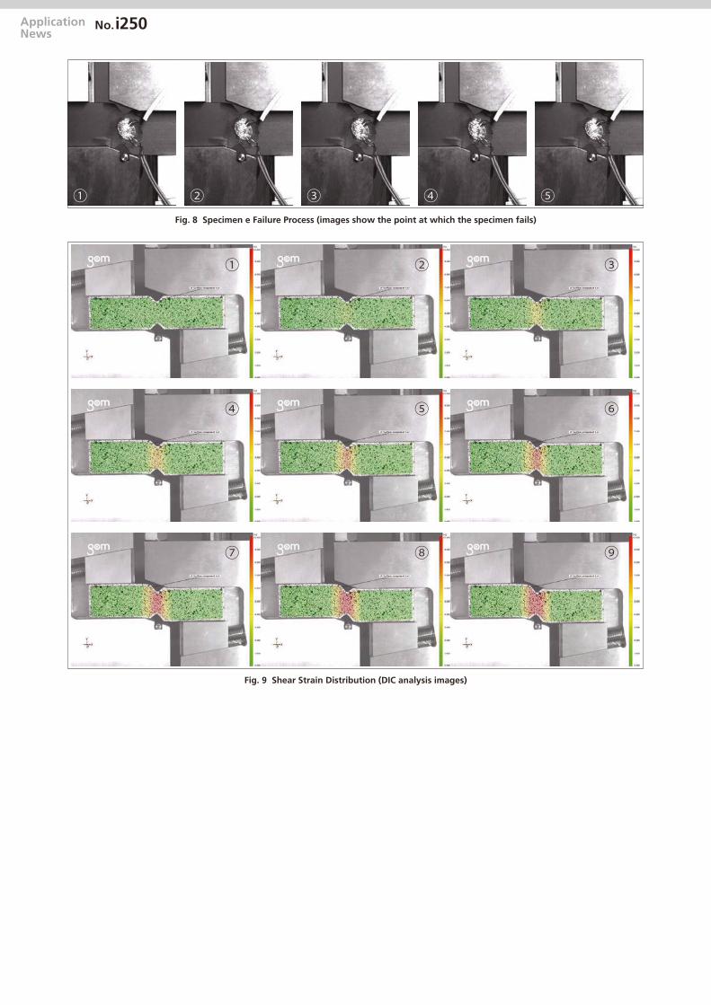
ApplicationNews
No.i250
① ② ③ ④ ⑤Fig. 8 Specimen e Failure Process (images show the point at which the specimen fails)
① ② ③
④ ⑤ ⑥
⑦ ⑧ ⑨
Fig. 9 Shear Strain Distribution (DIC analysis images)

ApplicationNews
No.
© Shimadzu Corporation, 2016
For Research Use Only. Not for use in diagnostic procedure.
This publication may contain references to products that are not available in your country. Please contact us to check the availability of these
products in your country.
The content of this publication shall not be reproduced, altered or sold for any commercial purpose without the written approval of Shimadzu.
Company names, product/service names and logos used in this publication are trademarks and trade names of Shimadzu Corporation or its
affiliates, whether or not they are used with trademark symbol “TM” or “®”. Third-party trademarks and trade names may be used in this
publication to refer to either the entities or their products/services. Shimadzu disclaims any proprietary interest in trademarks and trade names
other than its own.
The information contained herein is provided to you "as is" without warranty of any kind including without limitation warranties as to its
accuracy or completeness. Shimadzu does not assume any responsibility or liability for any damage, whether direct or indirect, relating to the
use of this publication. This publication is based upon the information available to Shimadzu on or before the date of publication, and subject
to change without notice.
www.shimadzu.com/an/
i250
First Edition: Aug. 2016
Conclusion
We used this test system to successfully implement the V-notched beam method (ASTM D5379). In addition to evaluating the basic properties of shear modulus and shear strength, integrating a Digital Video Extensometer into the test system enabled us to capture reference data that can be used to elucidate the mechanism of failure of CFRP, allowing strain analysis to be performed in terms of specimen failure mode and DIC analysis.

ApplicationNews
No.i251
Material Testing System
Shear Test of Composite Material
(V-Notched Rail Shear)
LAAN-A-AG-E016
Introduction
Carbon fiber reinforced plastic (CFRP) do not oxidize or rust and have a higher specific strength and stiffness than existing materials. Applications of CFRP are being investigated, with a focus on applications as industrial products that require strength and durability. Compared to exist ing homogeneous materials, composite materials like CFRP are anisotropic, and display complex failure behaviors as a result of tension, compression, bending, in-plane shear, out-of-plane shear, or a combination of these stresses arising from loading in the principal-axis direction. In recent years, use of CAE analysis in industry has become widespread since it can reduce numbers of prototypes and reduce the cost of new product development. Because values for each of the stress properties stated above are needed to i n c rea se p re c i s i on when p red i c t i ng p roduc t characteristics during product design, there is a strong demand for test methods able to evaluate pure failure behaviors in CFRP.There are various tests methods for evaluating composite materials. Of these methods, two commonly used in-plane shear test methods to test in the direction of fibers in fiber reinforced composite materials and to test textile laminated materials are the Iosipescu method (ASTM D5379) that applies an asymmetrical four-point bending load to a specimen cut with notches, and method (ISO 14129) that applies a ±45˚ tensile load on laminated materials. We used the V-notched rail shear method (ASTM D7078) that can be used to test in-plane shear. Because this method uses a large gauge area on the specimen, it can accommodate specimens without holes and CRFP laminate materials that have discontinuous fibers.
Measurement System
The equipment configuration is shown in Table 1. Information on the specimen prescribed by ASTM D7078 is shown in F ig. 1. The specimen is a [0/90]10s orthogonally laminated material made from Toray T800S prepreg that was molded in an autoclave. The specimen has a 31-mm evaluation area (see Fig. 1), and two-axis strain gauges attached at the mid-point between the V-notches (center of evaluation area) that are able to measure strain in –45˚ and +45˚ directions. Shear strain can be calculated by inserting the strain values obtained from these two strain gauges into equation (1). Shear strain is a property needed to evaluate the shear modulus.
. Equation (1)
: Shear strain
: Strain at +45˚
+45 +=ε –45εγγ
+45ε: Strain at –45˚–45ε
In this test, strain gauges were attached on both the front and rear of the specimen. Calculating the mean of outputs obtained from strain gauges on both sides allows for more accurate measurement of the shear strain in the specimen, and confirms whether shear
strain is being applied symmetrically on the front and rear of the specimen.
Testing Machine : AG-50kNX plusLoad Cell : 50 kNTest Jig : ASTM D7078 jigSoftware : TRAPEZIUM X (Single)Test Speed : 2 mm/min
Table 1 Test Conditions
Strain gauge
90˚
31
.0
56
.0
76.0
in gaugen gaugin
9090
aiStra
Evaluation area
Fig. 1 Shape of Specimen
Fig. 2 Testing Apparatus
Fig. 3 Imaging Apparatus

ApplicationNews
No.i251
The testing and imaging apparatus are shown in Fig. 2 and Fig. 3. Images captured using a TRViewX (Shimadzu Digital Video Extensometer) were gathered simultaneous to values obtained from the strain gauge outputs and specimen stress obtained by the testing apparatus. This made it easy to compare and evaluate images of the CFRP failure process against each specimen property values, something that was difficult to perform only with previous testing systems. Strain distribution can also be evaluated using digital image correlation (DIC, ARAMIS, GOMmbH) analysis of the images captured by TRViewX. To perform DIC analysis, paint must be sprayed on the specimen surface to create a random pattern on the front surface of the specimen.
Analytical Results
Each specimen property value obtained from this test is shown in Table 2. A photograph of the specimen after testing is shown in Fig. 4, a shear stress-normal strain curve is shown in Fig. 5 (strain values obtained from strain gauges), a shear stress-shear strain curve is shown in Fig. 6 (shear strain calculated from Equation (1)), and a shear stress-stroke curve is shown in Fig. 7. Table 2 shows that the results obta ined for each shear property were h ighly reproducible. Fig. 5 and Fig. 6 show that the same strain values were obtained from the front and rear strain gauges, and highly symmetrical shear strain was applied to the specimen.
Table 2 Test Results
Specimen Shear Modulus
[GPa]
Shear Strength
[MPa]
Test 1 4.63 121.72
Test 2 4.55 120.00
Test 3 4.58 120.05
Mean 4.59 120.60
Plastic deformationcaused by shearingPcc
Fig. 4 Specimen After Testing
-6 -5 -4 -3 -2 -1 0 1 2 3 4 5 6
10
20
30
40
50
60
70
80
90
100
Back +45˚Front +45˚
Back –45˚Front –45˚
Strain (%)
Sh
ear
Str
ess
(M
Pa)
0
Fig. 5 Shear Stress-Normal Strain Curve
0 1 2 3 4 5 6 7 8 9 100
10
20
30
40
50
60
70
80
90
100
BackFront
Sh
ear
Str
ess
(M
Pa)
Shear Strain (%)
Fig. 6 Shear Stress-Shear Strain Curve
0.0 0.5 1.0 1.5 2.0 2.5 3.0 3.5 4.0 4.5 5.0 5.5 6.00
10
20
30
40
50
60
70
80
90
100
110
120
130
140
Sh
ear
Str
ess
(M
Pa)
Stroke (mm)
Max
Fig. 7 Shear Stress-Stroke Curve
Failure of the specimen is shown in Fig. 8. A crack that appears c lose to the upper notch quickly propagates down toward the bottom notch during a simultaneous decrease in test force. Images of the shear strain distribution obtained by DIC analysis are shown in Fig. 9. The amount of strain occurring in the specimen is shown in terms of color, with low strain areas in cooler colors (black and blue) and high strain areas in warmer colors (orange and red). The images show that as the test progresses strain accumulates and is localized between the V-notches.

ApplicationNews
No.i251
Fig. 8 Specimen Failure Process (images show the point at which the specimen fails)
① ② ③ ④ ⑤
⑥ ⑦ ⑧ ⑨ ⑩
⑪ ⑫ ⑬ ⑭ ⑮Fig. 9 Shear Strain Distribution (DIC analysis images)

ApplicationNews
No.
© Shimadzu Corporation, 2016
For Research Use Only. Not for use in diagnostic procedure.
This publication may contain references to products that are not available in your country. Please contact us to check the availability of these
products in your country.
The content of this publication shall not be reproduced, altered or sold for any commercial purpose without the written approval of Shimadzu.
Company names, product/service names and logos used in this publication are trademarks and trade names of Shimadzu Corporation or its
affiliates, whether or not they are used with trademark symbol “TM” or “®”. Third-party trademarks and trade names may be used in this
publication to refer to either the entities or their products/services. Shimadzu disclaims any proprietary interest in trademarks and trade names
other than its own.
The information contained herein is provided to you "as is" without warranty of any kind including without limitation warranties as to its
accuracy or completeness. Shimadzu does not assume any responsibility or liability for any damage, whether direct or indirect, relating to the
use of this publication. This publication is based upon the information available to Shimadzu on or before the date of publication, and subject
to change without notice.
www.shimadzu.com/an/
i251
First Edition: Aug. 2016
Conclusion
We used this test system to successfully implement the V-notched rail shear method (ASTM D7078). In addition to evaluating the basic properties of shear modulus and shear strength, integrating a Digital Video Extensometer into the test system enabled us to capture reference data that can be used to elucidate the mechanism of failure of CFRP, allowing strain analysis to be performed in terms of specimen failure mode and DIC analysis.

■ Introduction As the result of recent progress of research and development, carbon fiber materials have been put to practical use in a wide range of implements, including space aircraft parts, sporting goods like golf club shafts and tennis rackets, structure materials that must transmit X-rays, and acoustic materials. A group of high-quality carbon fibers is further classified, according to its tensile strength, into several groups. One of these is a high-strength fiber group that features in excellent tensile strength; another is a high-elasticity fiber group characterized by high flexibility, but with a tensile strength of no more than around 2,000 MPa. As described above, data on mechanical properties are indispensable information for classifying fibers. The following is an example of tests for evaluation of physical behaviors under a compressive force applied to carbon fibers (single fibers) having different tensile strength levels with Shimadzu Micro Compression Testing Machine MCT.
■ Testing Conditions (1) Testing mode: compression test (2) Testing load: 200 gf (3) Loading rate constant: 1 (4,230 gf/sec.) (4) Calculation of strength: Compression strength is calculated by the following equation. *1
𝑆𝑆𝑆𝑆𝑆𝑆𝑆𝑆 = 2 ∙ 𝑃𝑃𝑃𝑃 ∙ 𝜋𝜋𝜋𝜋 ∙ 𝑑𝑑𝑑𝑑 ∙ 𝐿𝐿𝐿𝐿
where: ST: tensile strength (kg/mm2) P: compression strength (kgf) d: diameter of fiber (mm) L: length of fiber (mm) Note *1: from JIS A1113-1976 Method of tests for splitting tensile strength of concrete
Material Testing System MCT
Compression-Rupture Test of Carbon Fibers with Different Tensile Characteristics Shimadzu Micro Compression Testing
No. SCA_300_037

■ Test Piece (1) Name: Carbon fibers (PAN type
carbon fibers)
(2) Types: 1 (high-ductility type)
2 (high-strength type)
3 (ultra-high elasticity type)
(3) Shape: See Fig. 1
Fig. 1 A Microscopic photograph of Test Piece before Test
Fig. 2 A Microscopic photograph of Test Piece after Test
Fig. 3 Load- Deformation Curves of High Ductility Samples
Fig. 4 Load- Deformation Curves of High Ductility Samples
Fig. 5 Load- Deformation Curves of High Ductility Samples
No. SCA_300_037
Type of test piece Compression-rupture strength(kgf/mm2)
Standard deviation (kgf/mm2)
High-ductility type 149.90 3.23 High-strength type 151.09 6.34 Ultra-high elasticity type 68.87 4.37
Table 1 Results of Compression-Rupture Test of Carbon Fibers
Note: The length of the indenter diameter (50 mm) was used for the length of fiber because the test piece was extraordinarily long.
■ Test Results Table 1 shows a summary of test data, and Figs. 2-4 show the compression-rupture strength and the overlapping view of load-deformation curves for each test piece. The difference of behavior between test pieces are observable in the load-deformation curves of Figs. 2-4. The test pieces of the high-ductility type and the high-strength type have similar compression-rupture strength, while the ultra-high elasticity type has a remarkably low compression-rupture strength. (Refer to Table 1) Admitting some deviation among the test data as a result of the surface conditions of the test pieces, the test results ensure that this testing machine is useful and effective for evaluation of mechanical properties of single fibers, provided that data are processed statistically. * Please be advised that data obtained before the implementation of the current Weights and Measures Law may be presented in terms of gravimetric unit.
No. SCA_300_037

CFRP (carbon fiber reinforced plastic) has attracted attention as a high-performance composite material with high strength and rigidity, yet low in weight, and is being applied in various fields, such as for aircraft, railroad vehicles, automobiles and civil engineering. This example describes evaluating the characteristics of a flat plate specimen of CFRP material when a tensile load is applied (tensile test) and observing the fracture status. Tensile testing consisted of static testing of material strength and measuring the modulus of elasticity using a precision universal testing machine. In addition, high-rate tensile impact test was also performed. In the latter case, a high-speed video camera was used to record specimen fracture, which allowed capturing image data of the instant the CFRP material fractured. ■ Test specimen The tensile test specimen tested in this example is shown in figure 1. Included 50 mm long CFRP tabs attached to both ends of the CFRP strip with thermosetting resin adhesive. Reinforcing the grip area with tabs ensures a stable tensile test with good reproducibility.
Figure 1: CFRP test specimen
Specimen details are as follows: 1) Material: unidirectional CFRP 2) Shape: strip (with tabs on both ends) 3) Specimen dimensions: for static tensile
testing 200(L) x 12.5(W) x 1(T) mm. For recording image of impact fracture 70(L) x 6.25(W) x 0.3(T) mm
■ Static tensile test A strain gauge type extensometer was attached to the specimen and a tensile test was performed using a precision testing machine. The extensometer was removed when strain exceeded the elasticity measurement range. It is also possible to measure strain by affixing a strain gauge instead of an extensometer. Tensile test parameters are indicated below. (1) Tensile rate: 10 mm/min (2) Grip distance: 100 mm (3) Test force detection: 50 KN load cell (4) Extensometer gauge length: 50 mm (5) Elasticity calculation range: 5/10,000 to
25/10,000 strain
Figure 2: Static test results
Material Testing System AG-X
Observation of fracture in CFRP tensile test
No. SCA_300_059
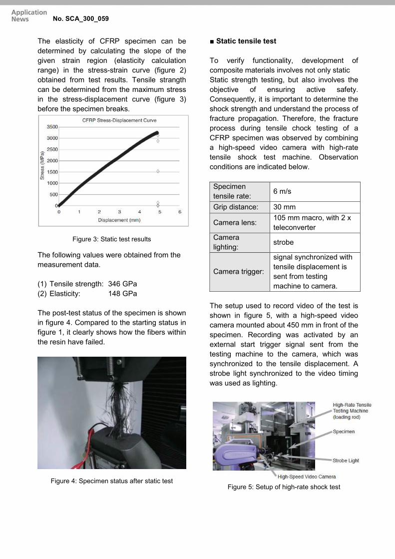
The elasticity of CFRP specimen can be determined by calculating the slope of the given strain region (elasticity calculation range) in the stress-strain curve (figure 2) obtained from test results. Tensile strangth can be determined from the maximum stress in the stress-displacement curve (figure 3) before the specimen breaks.
Figure 3: Static test results
The following values were obtained from the measurement data. (1) Tensile strength: 346 GPa (2) Elasticity: 148 GPa
The post-test status of the specimen is shown in figure 4. Compared to the starting status in figure 1, it clearly shows how the fibers within the resin have failed.
Figure 4: Specimen status after static test
■ Static tensile test To verify functionality, development of composite materials involves not only static Static strength testing, but also involves the objective of ensuring active safety. Consequently, it is important to determine the shock strength and understand the process of fracture propagation. Therefore, the fracture process during tensile chock testing of a CFRP specimen was observed by combining a high-speed video camera with high-rate tensile shock test machine. Observation conditions are indicated below. Specimen tensile rate: 6 m/s
Grip distance: 30 mm
Camera lens: 105 mm macro, with 2 x teleconverter
Camera lighting: strobe
Camera trigger:
signal synchronized with tensile displacement is sent from testing machine to camera.
The setup used to record video of the test is shown in figure 5, with a high-speed video camera mounted about 450 mm in front of the specimen. Recording was activated by an external start trigger signal sent from the testing machine to the camera, which was synchronized to the tensile displacement. A strobe light synchronized to the video timing was used as lighting.
Figure 5: Setup of high-rate shock test
No. SCA_300_059

Using this test configuration, a load was applied to the CFRP specimen according to the parameters indicated above and a high-speed camera captured the instant of fracture, at 250.000 frames per second. This image data shown in figure 6. This shows 8 consecutive frames, from (1) TO (8), with an interval of 4 microseconds between each frame. This camera features highly detailed image resolution of 312
horizontal by 260 vertical pixels that is constant, regardless of the frame rate. This example shows, combining a high-speed video camera and material testing machine makes it possible to evaluate material properties and observe fracture behavior at the same time. This enables supporting a wide range of material development applications, from developing individual functionally enhanced resins to developing composite materials.
Figure 6: Images of specimen during fracture
No. SCA_300_059

C225-E032
Ultrasonic Fatigue Testing System Effective for Gigacycle Fatigue Tests
With fatigue tests of high-strength steels, it is evident that internal fracture (fish-eye fracture), which is caused by inclusions and other micro defects, occurs at 107 cycles or more, a value considered the conventional fatigue limit.An ultrasonic fatigue testing system is extremely effective when performing this sort of gigacycle fatigue test. (With a 100 Hz fatigue testing system, this would take 3 years, but if a 20 kHz ultrasonic fatigue testing system is used, testing can be completed in one week.)
Actual components are rarely used under conditions in which the average stress is zero. Despite this, the USF-2000A, a standard ultrasonic fatigue testing system, can only perform testing under zero average stress conditions.Using an ultrasonic fatigue testing system equipped with an average stress loading mechanism, gigacycle fatigue tests can be performed with average tensile stress loaded.
Ultrasonic Fatigue Testing System with an Average Stress Loading Mechanism
Stressdistribution
AG-X5kNAverage stress loading
High-rigidity booster
Horns
High-rigidity booster
5 kN load cellAverage stress measurement
Converter(Piezo actuator)
Strain GaugeSamples
DisplacementStress
System Appearance
For Gigacycle Fatigue Tests with Average Stress Loaded

© Shimadzu Corporation, 2016First Edition: August 2016
For Research Use Only. Not for use in diagnostic procedure. This publication may contain references to products that are not available in your country. Please contact us to check the availability of these products in your country.Company names, product/service names and logos used in this publication are trademarks and trade names of Shimadzu Corporation or its affiliates, whether or not they are used with trademark symbol “TM” or “®”. Third-party trademarks and trade names may be used in this publication to refer to either the entities or their products/services. Shimadzu disclaims any proprietary interest in trademarks and trade names other than its own.
The contents of this publication are provided to you “as is” without warranty of any kind, and are subject to change without notice. Shimadzu does not assume any responsibility or liability for any damage, whether direct or indirect, relating to the use of this publication.www.shimadzu.com/an/
Ultrasonic resonance systemPower supply, converter, booster (1 pair), horn (1 pair)
Personal computer(OS Windows 7) ADA/PIO interface board
SoftwareUltrasonic test control measurement software
Cooling systemAir dryer, air piping• A separate 140 L/min air source is required.
5 Strain meter unit (option)
6 AG-X plus Autograph 5 kN + 250 extension
7 Average stress loading mechanism
1
2
3
4
Main Speci�cations
1) Test Frequency: 20 kHz ± 500 Hz
• The recommended test range is 20 kHz ± 30 Hz.• The test frequency is determined by the resonance frequency of the sample.
2) Horn End Face Amplitude
Min. approx. ±10 μmMax. approx. ±50 μm
• The minimum and maximum amplitudes are the end face amplitude values at amplitude outputs of 20 % and 100 % respectively. Accordingly, the minimum and maximum amplitude values will change somewhat depending on the shape of the sample.
4) Average Stress
Max. 1.5 kN (tensile only)
3) Test Stress
Standard circular tapered sampleStress Min. 237 MPa Max. 1186 MPa• The test stress range can be changed by changing the sample shape.• The minimum and maximum values are calculated with the end face amplitude values of 10 μm and 50 μm respectively.• These are the values when the stress is within the elasticity range.
Standard Circular Tapered Sample
Surface of the Fatigued Fracture Originating from the Inclusion
Center hole can remain
Center holecan remain
Components

ApplicationNews
No.
LAAN-A-AG-E009
Material Testing System
Tensile Test for Metallic Materials Using Strain Rate Control and Stress Rate Control
i244International standards for tensile testing of metallic materials have been revised as specified in ISO 6892 and JIS Z2241, such that strain rate control, where strain is measured with an extensometer, has recently been added as a test item to the current stress rate control method, in which a load is applied to a material until its yield point is reached. As a result, it can be assumed that there will be situations where both stress rate control and strain rate control tensile testing of
metallic materials will be required.Here, we introduce examples of strain rate control and stress rate control tensile testing of metallic samples, including cold-rolled steel, austenitic stainless steel, aluminium alloy and brass, according to ISO 6892, using the Shimadzu Autograph AG-50kNX Precision Universal Tester, and the SSG50-10H strain gauge type one-touch extensometer (Fig. 1, Fig. 2).
Table 1 Test Specimens
Information on the sample specimens are shown in Table 1, and the test conditions are shown in Table 2.
n Introduction
n Specimens and Test Conditions
Fig. 1 Overview of Universal Testing System Fig. 2 Specimen and Jigs for Tensile Testing
Sample Name A B C D
Material Cold-rolled steel Stainless steel (austenitic) Aluminium alloy Brass
Sample size
Width 25 mm, thickness 1 mm, gauge length 50 mm, parallel length 60 mm(JIS Z 2241 No. 5 test specimen)
Gauge length
50 mm
Parallel length60 mm
Width 25 mm

Table 2 Test Conditions
1) Load cell capacity 50 kN
2) Jig 50 kN Non-shift wedge type grips (file teeth for flat specimen)
3) Test speed See Table 3
4) Test temperature Ambient temperature
5) Software TRAPEZIUMX (single)
Fig. 3 shows an image diagram of the test speed, and Table 3 and Table 4 show the applicable test speeds for the strain control and stress control tests, respectively.
Table 3 Test Strain Rate (based on strain rate control)
V1: Strain rate 0.00025/s (1.5 %/min)
V2: Strain rate 0.00025/s (1.5 %/min)
V3: Predicted strain rate 0.0067/s (40 %/min)
Table 4 Test Stress Rate (based on stress rate control)
V1: Stress rate 10 MPa/s
V2: Strain rate 0.00083/s (5 %/min)
V3: Predicted strain rate 0.0067/s (40 %/min)
Table 5 Test results (Average n = 3)
Sample NameElastic
Modulus (GPa)
0.2 % Proof Strength
(MPa)
Tensile Strength
(MPa)
Elongation at Break
(%)
A (cold-rolled steel) 194 185.5 341.5 43.3
B (stainless steel) 200 278.5 660.8 55.0
C (aluminum) 71 170.1 236.3 13.0
D (brass) 109 193.1 398.1 49.1
(A): Upper yield point (or its corresponding point)(B): Upper limit of strain measurement (point after proof strength point)
Note 1) Strain rate refers to the amount of increase in strain, obtained using an extensometer to measure the gauge length of a test specimen, per unit time.
Note 2) Predicted strain rate was obtained using the displacement of the testing machine crosshead at each point in time and the test specimen's parallel length. Thus, it is defined as the increase in strain of the specimen's parallel length per unit time.
Fig. 3 Image of Test Strain Rate
Strain (%)(A) (B)
Stre
ss (M
Pa)
V2
V1
V3
F ig. 4 shows a d iagram of the st ress – s t roke displacement for each sample using strain-rate control, and Table 5 shows their characteristic values. In Fig. 4, the point at which the stress becomes discontinuous, as indicated by the jump in the stress-stroke displacement curve, corresponds to the point at which the strain rate is switched.
n Test Results
Fig. 4 Test Results for Each Metallic Material (stress-stroke curve based on strain rate control)
Stroke Displacement (mm)
Stre
ss (M
Pa)
800
700
600
500
400
300
200
100
00 20 40 60 80
ABCD

Fig. 6 Test Results (stress-stroke curve based on stress rate control)
Fig. 5 (a) – (d) shows the strain rate and predicted strain rate obtained from tensile testing of the respective metallic materials using strain rate control. The red solid lines show the strain rate, the blue solid lines the predicted strain rate, and the black broken lines show the stress. In addition, the green dotted lines represent the permissible value ±20 % relative tolerance in the strain rate control (as specified in ISO 6892). As for the actual load rate, it is clear that the values are well
within the permissible strain rate control range, indicating excellent strain rate control. Regarding samples A and B, displacement is measured up to 2 % of the gauge length using an extensometer. In the case of samples C and D, the strain measured using an extensometer was only up to 0.8 %, because of the appearance of serration when strain corresponding to about 1 % was applied.
Fig. 6 shows the stress-stroke displacement curve diagram obtained from tensile testing of each of the metallic materials using stress rate control, and the characteristic values are shown in Table 6.
Fig. 5 (a) Test Results (Sample A)
0 20 40 60 80 100 120 1400
100
200
300
400
500
600
700
800Stress
10-5
10-4
10-3
10-2
10-1
100
Strain rate control region
Predicted strain rateStrain rate
Predicted strain rate control region
Stre
ss (M
Pa)
Stra
in R
ate,
Pre
dict
ed S
trai
n Ra
te (S
-1)
Time (s)
Fig. 5 (b) Test Results (Sample B)
0 20 40 60 80 100 120 140
Strain rate control region
StressPredicted strain rateStrain rate
0
100
200
300
400
500
600
700
800
10-5
10-4
10-3
10-2
10-1
100
Predicted strain rate control region
Stre
ss (M
Pa)
Stra
in R
ate,
Pre
dict
ed S
trai
n Ra
te (S
-1)
Time (s)
Fig. 5 (c) Test Results (Sample C)
0 20 40 60 80 100 120 140
Strain rate control region
StressPredicted strain rateStrain rate
0
100
200
300
400
500
600
700
800
10-5
10-4
10-3
10-2
10-1
100
Predicted strain rate control region
Stre
ss (M
Pa)
Stra
in R
ate,
Pre
dict
ed S
trai
n Ra
te (S
-1)
Time (s)
Fig. 5 (d) Test Results (Sample D)
0 20 40 60 80 100 120 140
Strain rate control region
StressPredicted strain rateStrain rate
0
100
200
300
400
500
600
700
800
10-5
10-4
10-3
10-2
10-1
100
Predicted strain rate control region
Stre
ss (M
Pa)
Stra
in R
ate,
Pre
dict
ed S
trai
n Ra
te (S
-1)
Time (s)
Stroke Displacement (mm)
Stre
ss (M
Pa)
800
700
600
500
400
300
200
100
00 20 40 60 80
ABCD

For Research Use Only. Not for use in diagnostic procedures.The contents of this publication are provided to you “as is” without warranty of any kind, and are subject to change without notice. Shimadzu does not assume any responsibility or liability for any damage, whether direct or indirect, relating to the use of this publication.
First Edition: January, 2012
www.shimadzu.com/an/ © Shimadzu Corporation, 2012
Fig. 7 (a) – (d) shows the strain rate and predicted strain rate obtained from tensile testing of the respective metallic materials using stress rate control. The pink
solid lines show the stress rate, the blue solid lines the predicted strain rate, and the black broken lines show the stress.
It is clear that at the set rates, suitably stable data could be acquired for both stress rate and predicted strain rate.The above results demonstrate that in the tensile testing of the various types of metallic materials using the Shimadzu Autograph AG-50kNX Precision Universal Tester, the strain rate control values were well within the range of the permissible values (± 20 %) specified in ISO 6892. Similarly, stable testing using stress rate control was also achieved. When using typical universal
testing machines, testing control methods other than the crosshead rate control, e.g. strain rate control and stress rate control, normally require burdensome adjustment of the control gain depending on the material being tested. However, with this instrument, strain rate control and stress rate control in tensile testing of any metallic material are easily conducted because the gain is adjusted automatically (auto-tuning feature).
Fig. 7 (a) Test Results (Sample A)
0
10
20
30
40
50
60
70Stress × 0.1Stress rate
10-5
10-4
10-3
10-2
10-1
100
Predicted strain rate
0 20 40 60 80 100 120 140
Stre
ss R
ate
(MPa
/s),
Stre
ss (M
Pa)
Pred
icte
d St
rain
Rat
e (S
-1)
Time (s)
Fig. 7 (b) Test Results (Sample B)
Stress × 0.1Stress rate
Predicted strain rate
0
10
20
30
40
50
60
70
10-5
10-4
10-3
10-2
10-1
100
0 20 40 60 80 100 120 140
Stre
ss R
ate
(MPa
/s),
Stre
ss (M
Pa)
Pred
icte
d St
rain
Rat
e (S
-1)
Time (s)
Fig. 7 (c) Test Results (Sample C)
Stress × 0.1Stress rate
Predicted strain rate
0
10
20
30
40
50
60
70
10-5
10-4
10-3
10-2
10-1
100
0 20 40 60 80 100 120 140
Stre
ss R
ate
(MPa
/s),
Stre
ss (M
Pa)
Pred
icte
d St
rain
Rat
e (S
-1)
Time (s)
Fig. 7 (d) Test Results (Sample D)
Stress × 0.1Stress rate
Predicted strain rate
0
10
20
30
40
50
60
70
10-5
10-4
10-3
10-2
10-1
100
0 20 40 60 80 100 120 140
Stre
ss R
ate
(MPa
/s),
Stre
ss (M
Pa)
Pred
icte
d St
rain
Rat
e (S
-1)
Time (s)
Table 6 Test Results (Average n = 3)
Sample NameElastic Modulus
(GPa)0.2 % Proof Strength
(MPa)Tensile Strength
(MPa)Elongation at Break
(%)
A (cold-rolled steel) 194 193.3 349.3 42.0
B (stainless steel) 205 290.7 687.0 54.8
C (aluminum) 69 177.0 233.5 12.6
D (brass) 112 196.7 405.5 48.8

Recent years have seen intensive requests for engineering materials with higher function ability and longer life, and as a result, surface treatment for such materials has become popular. Under this circumstance, hardness testers with micro load are enjoying an
increasing demand. In this regards, a test report is herein introduced on the hardness distribution measured from the sample surface toward depth direction with an interval of 2 μm, using Shimadzu Dynamic Ultra Micro Hardness Tester Model DUH.
■ Test Parameters 1) Sample: plating layer on a metal plate (See
Fig. 1) 2) Indenter: tip angle 136°, square pyramid
indenter (Vickers indenter) 3) Measuring mode: load-load-hold test (mode 1) 4) Test load: 2.0 gf 5) Loading speed: 0.029 gf/sec. 6) Load hold-time: 10 sec.
■ Test Method 1) Vickers Hardness Testing procedures, the distance between the indentation center and the sample edge shall be 2.5 time the diagonal length or more (the diagonal length is 2.6 μm or less). The test load was determined in accordance with this specification, and the tests were performed near the mid depth of the plating layer.
2) Hardness distribution measurements were performed at the location and with the depth intervals of 2 μm starting from the sample surface as shown in Fig. 2
Fig. 1
Material Testing System DUH
A hardness measurement of surface treatment layer on a steel sample using Shimadzu Dynamic Ultra Micro Hardness Tester, Model DUH No. SCA_300_035

Fig. 2
■ Test Results The average of five measurements is shown in Table 1, and the load-indentation depth curve is in Fig. 3
Test Load (gf)
Depth (µm)
Dynamic Hardness DHV
2,001 0,206 1065
Table 1 Hardness Test Result
Dynamic Hardness was determined by the following formula:
𝐷𝐷𝐷𝐷𝐷𝐷𝐷𝐷𝐷𝐷𝐷𝐷 =37,838 ∙ 𝑃𝑃𝑃𝑃
ℎ2
Where:
DHV: Dynamic hardness by Vickers Indenter
P: Test Load (gf)
H: Indentation depth (µm)
Fig. 3 Load-Indentation depth curve
■ Test Results Result of five tests with a depth interval of 2 μm is listed in Table 2.
Test Load (gf) DHV
1 2 3 4 5 6
2,0 847 1001 1070 1103 966 925
Table 2 Hardness Distribution
..
0
0,5
1
1,5
2
0 0,5 1
Load
(gf)
Depth (µm)
No. SCA_300_035

■ Dynamic hardness was determined by the same formula as item 1) above. The Relation of depth and hardness is shown in Fig. 4.
Fig. 4
Fig. 4 indicates a tendency that hardness increases as depth increases, reaches the max. at mid depth of the plating layer, and decreases thereafter.
0
200
400
600
800
1000
1200
0 2 4 6 8 10 12 14
Achs
entit
el
Hardness (DHV)
No. SCA_300_035

曲げひずみ
曲げ応
力
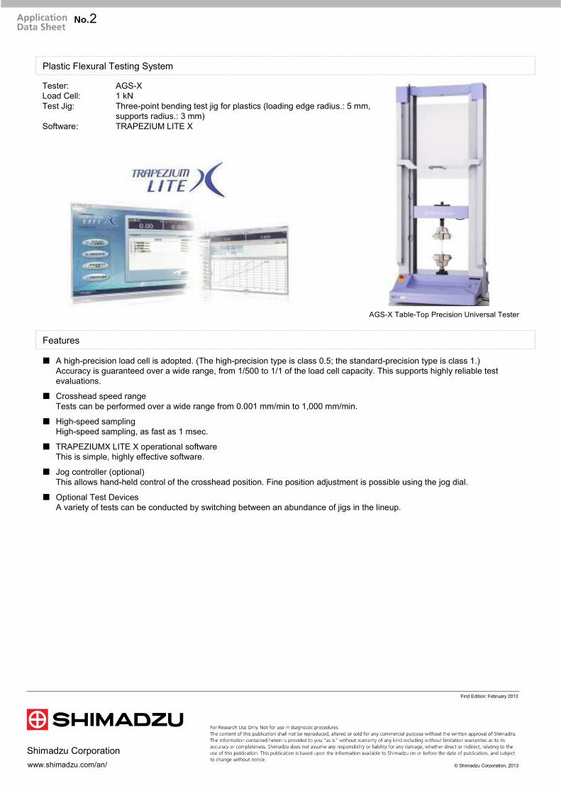

ひずみ
応力


変位
試験
力


変位
試験
力


縦ひずみ
横ひずみ
応力
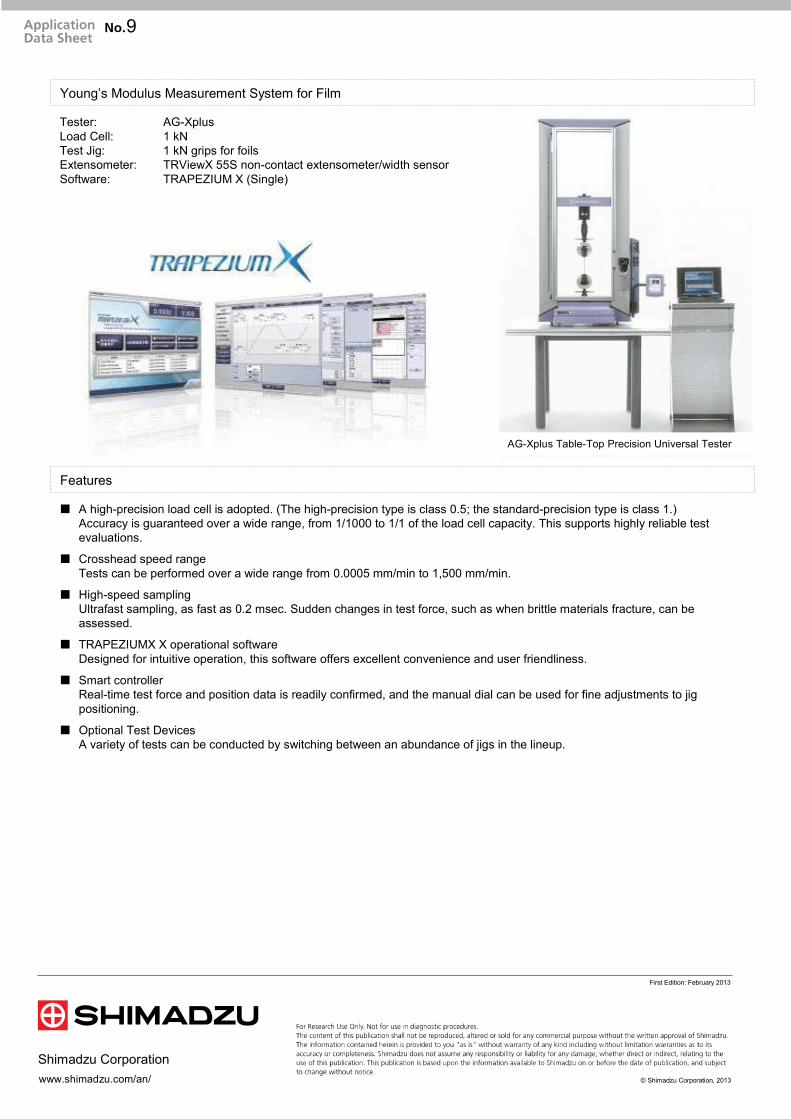

3. Biomaterials and Medical Industry

3. Biomaterials and Medical Industry
DEVELOPMENT OF ADVANCED MEDICAL TREATMENTS
World population was just two billion in 1927, but reached seven billion in 2011 and is expected to be ten billion by the end of the 21st century. At the same time, so-called advanced countries are becoming aging societies. This dramatic growth in population and life-expectancy is said to result from more sophisticated medicine, which in turn will require more advanced medical technology.
The medical equipment and biomaterials industries have expe-rienced a vast number of innovations and developments over the past decade. In addition, great strides have been made in materials and technologies; therapeutic strategies and surgical techniques have progressed dramatically. For instance, a bro-ken femur can now be replaced by an implant, and inserting small metal stents weighing just a few grams into the neuro-vascular system can prevent strokes due to plaque or arterial stenosis.
To guarantee the safety and efficacy of medical equipment and technologies in the wake of such medical breakthroughs, active efforts are being made to reinforce evaluation criteria and the regulations governing the standardization of measur-ing instruments and test methods. Medical equipment manu-facturers and research organizations around the world are conducting research and development into medical equipment based on mechanical properties evaluation and finite element analysis.
Shimadzu applies its technical expertise cultivated through physical testing, quality control and full-scale testing in mate-rials development to the fields of leading-edge medicine and biomaterials evaluation.

3. Biomaterials and Medical Industry
No.ei252 Orthodontic implant fatigue testing
SCA_300_058 Measurement of press-trough package force and tablet break force

ApplicationNews
No.i252
Material Testing System
Orthodontic Implant Fatigue Testing
LAAN-A-SB-E003
Introduction
Dental implantation normally refers to a method of treatment that involves embedding a titanium implant in the jaw bone and fitting an artificial tooth onto this implant to return the function and aesthetic appearance of the original tooth. Orthodontic implantation uses implant technology to affix artificial material into bone. Embedding artificial material into bone has advantages of orthodontic therapies that use implants, such as being able to secure a stronger anchor, increasing the range of movement of the teeth, increasing the likelihood of using therapies that do not require tooth removal, and increasing the scope of non-surgical orthodontic therapy. However, fluoride solutions used in mouthwash can have a negative effect on the durability of titanium implants. Consequently, fatigue testing of orthodontic implants must be performed in solution so its effect can be determined and more durable orthodontic implants developed. We performed fatigue testing of an orthodontic implant in pure water at 37 ˚C, and report the results.
Measurement System
The Electromagnetic Force Fatigue and Endurance Test System MMT-101NV-10 was used for testing. Testing was performed in pure water at 37 ˚C using a thermostatic water immersion test unit. Testing was performed as shown in Fig. 1, and the test equipment used is shown in Table 1.
Indenter
Cantilever bending jig
Implant
Fig. 1 Test Overview
Testing machine : MMT-101NV-10Load Cell : 100 NJig : Implant cantilever bending jigTank : Thermostatic water immersion test unit
Table 1 Experimental Equipment
Results
(1) Static testingFirst, static testing was performed to determine the loading level for fatigue testing. Test conditions are shown in Table 2, and the static test results are shown in Fig. 2. Based on static test results, the mean maximum strength was 35.4 N.
Testing Speed : 5 mm/minTest Environment : Room temperature, in airNumber of Tests : n = 5
Table 2 Test Conditions
00
5
10
15
20
25
30
35
40
1 2
Displacement [mm]3 4
Fo
rce
[N
]
Fig. 2 Results of Static Testing
(2) Fatigue testingThe loading level for fatigue testing was determined based on the static test results. The test conditions used in fatigue testing are shown in Table 3.
Max. Force : 30, 25, 20, 15, 12.5, 11, 10, 9, 8, 7Stress Ratio : 0.1Frequency : 10 HzTest Environment : 37 ˚C, in pure waterMax. Number of Repetitions : 5,000,000Number of Tests : n = 1
Table 3 Test Conditions

ApplicationNews
No.
© Shimadzu Corporation, 2016
For Research Use Only. Not for use in diagnostic procedure.
This publication may contain references to products that are not available in your country. Please contact us to check the availability of these
products in your country.
The content of this publication shall not be reproduced, altered or sold for any commercial purpose without the written approval of Shimadzu.
Company names, product/service names and logos used in this publication are trademarks and trade names of Shimadzu Corporation or its
affiliates, whether or not they are used with trademark symbol “TM” or “®”. Third-party trademarks and trade names may be used in this
publication to refer to either the entities or their products/services. Shimadzu disclaims any proprietary interest in trademarks and trade names
other than its own.
The information contained herein is provided to you "as is" without warranty of any kind including without limitation warranties as to its
accuracy or completeness. Shimadzu does not assume any responsibility or liability for any damage, whether direct or indirect, relating to the
use of this publication. This publication is based upon the information available to Shimadzu on or before the date of publication, and subject
to change without notice.
www.shimadzu.com/an/
i252
First Edition: Jul. 2016
Test results are shown in Fig. 3. Fig. 3 shows that at a maximum force 11 N the number of cycles to failure was < 10,000, and there was no particular increase in the number of cycles to failure. At test forces 10 N, the maximum force fell and the number of cycles to failure increased substantially. At a maximum force of 7 N, failure did not occur at < 5,000,000 cycles.
35
Ma
x.
Fo
rce
[N
]
30
25
20
15
10
5
0
1.E+01 1.E+02 1.E+03 1.E+04
Number of cycles
1.E+05 1.E+06 1.E+07
Fig. 3 S-N Curve
Conclusion
We performed cantilever bending fatigue testing of an orthodontic implant at 37 ˚C in pure water. The orthodontic implant we tested had a small number of cycles to failure at maximum forces 11 N ( 31 % of static strength), but this number of cycles to failure increased at forces 10 N ( 28 % of static strength). We plan to perform more fatigue testing in fluoride compound-containing mouthwash solution. This report shows that Shimadzu's test system can be used to perform cant i lever bending fat igue test ing of orthodontic implants in solution, and may be used for the development and evaluation of orthodontic implants.

Many tablets and capsules are packaged in thin metallic (aluminum etc.) and plastic materials. This type of package is referred to as a PTP (press trough package) or PTP sheet, and serves to protect the contained tablets and capsules and facilitate handling of the contents. Therefore, quality control is necessary to ensure that the package does not peel excessively, and that the tablet is not too difficult to dispense.
Figure 1: PTP packaged tablets
Figure 2: Testing machine (EZ-SX)
Here, using the Shimadzu EZ-X compact table-top universal testing machine and the TrapeziumX material testing software, we introduce an example of the adhesive strength of the PTP package, in addition to the force required to break a tablet in half. ■ Press-Dispense test for PTP packaged tablets As shown in figure 4, the test was performed by pushing the tablet out of the PTP package using an upper 10 mm spherical press jig at a test speed of 50 mm/min, and a fix platform below. In this case the result obtained was a maximum test force mean value of 24.3 N. The judgment as to whether or not the tablet is easy to push out can be obtained from the maximum test force, which is applicable to product development and quality control.
Figure 3: Results of press-dispense test
Material Testing System EZ-X
Measurement of Press-Trough Package Force and Tablet Break Force
No. SCA_300_058

Figure 4: View of testing machine during measurement
■ Peel test for PTP packages
Figure 5: Results of peel test
Figure 6: Testing machine during measurement
As shown in figure 6, using a 100N pantograph type jigs above and fixing platform below, we performed the test by peeling the aluminum foil off from the underside of the PTP package at a test speed of 50 mm/min. peeling began at about 0.3 N, and at the package edge the force was about 3 N.
■ Break test of tablets
Figure 7: Results of break force test
Figure 8: Testing machine during measurement
No. SCA_300_058

■ Summary Some tablets have a groove in the center, allowing each to be taken whole by adults or via a half dose by children. Accordingly, it must be able to be broken in half using some suitable degree of force. As a suitable method of simulating this breaking in half, that tablet was placed above the bend test jig supports (5 mm distance between supports), and measurement was conducted at a test speed of 0.5 mm/min until the tablet broke. As shown in the measurement result graph of figure 7, the force required to break the tablet in half (mean value of maximum test force) was about 24 N. By using this kind of measurement, the depth of the tablet center groove can be optimized so that the tablet is easily and accuratelly broken in half. Thus, by combining the Shimadzu EZ-X compact table-top universal testing machine with the abundant selection of test jigs, test force evaluation of drug products including the packaging material can be conducted easily.
No. SCA_300_058

4. Composite Industry

4. Composite Industry
GROWING USE OF COMPOSITE MATERIALS
Composites combine different materials to achieve greater specific strength than is available from a single material. The evaluation of fundamental mechanical properties is essential for new materials. Ongoing standardization of sample shapes and test methods is intended to improve the stability of mate-rial quality while enhancing reliability.
Fiber-reinforced plastics (FRP) are typical composite materials. Among these are glass-fiber-reinforced plastics (GFRP) which are widely used for aircraft wing fillets, fairings, control surfaces, radomes, wing tips and cabin floors. Carbon-fiber-reinforced plastics (CFRP) combine plastics with carbon fibers having high specific modulus of elasticity and specific strength; they are applied in important components such as aircraft wings and center wing boxes as well as horizontal and vertical stabilizers.
Aircraft are designed to meet the requirements indicated in the design standards. Inspection and testing of aircraft struc-ture and strength are performed at the manufacturing stage, and flight testing is conducted to confirm the performance and flying quality of the completed aircraft. Testing includes static and fatigue testing at the materials development stage, endur-ance testing of all parts and components, and impact testing to evaluate the fast fracture characteristics of the materials.
In recent years, it has become more important to observe fracture behavior. High-speed video cameras are now com-monly used to perform more sophisticated evaluations through synchronized observations of the tested material behavior and the S-S curve.

4. Composite Industry
No_ei254 Compression after impact testing of composite
No_ei255 Compression testing of composite materials
No.36 Evaluating the fatigue strength of GFRP materials
No.30 Evaluating the strength of carbon fiber reinforced plastics (CFRP)
No.39 Evaluation of open-hole CFRP
No.i247 DIC analysis material testing by strain distribution visualization
No.8 Flexural testing of CFRP boards
No.16 Tensile testing of carbon fiber
No.31 Materials testing using digital image correlation
No.37 Observing the failure of open-hole CFRP samples in tensile tests
No.38 Observing the fracture of unidirectional CFRP in static tensile testing
No.ei256A Open-hole compression testing of composite material
No.ei250 Shear test of composite material (V-notched beam)
No.ei251 Shear test of composite material (V-notched rail shear)
SCA_300_037 Compression-rupture test of carbon fibers with different tensile characteristics Shimadzu micro compression testing machine MCT
SCA_300_055 Viscosity evaluation of thermoplastic resins (GFRP)
SCA_300_056 Viscosity evaluation of thermoplastic resins (GFRP)
SCA_300_059 Observation of fracture in CFRP tensile test E001HPV

ApplicationNews
No.i254
Material Testing System
Compression After Impact Testing of Composite
Material
LAAN-A-AG-E018
Introduction
Carbon fiber reinforced plastic (CFRP) has a higher specific strength and rigidity than metals, and is used in aeronaut ics and as t ronaut ics to improve fue l consumption by reducing weight. However, CFRP only exhibits these superior properties in the direction of its fibers, and is not as strong perpendicular to its fibers or between its laminate layers. When force is applied to a CFRP laminate board, there is a possibi l ity that delamination and matrix cracking will occur parallel to its fibers. Furthermore, CFRP is not particularly ductile, and is known to be susceptible to impacts. When a CFRP laminate board receives an impact load, it can result in internal matrix cracking and delamination that is not apparent on the material surface. There are many situations in which CFRP materials may sustain an impact load, such as if a tool being dropped onto a CFRP aircraft wing, or small stones hitting the a CFRP wing during landing. Consequently, tests are required for these scenarios. One of these tests is compression after impact (CAI) testing. CAI testing involves subjecting a specimen to a prescribed impact load, checking the state of damage to the specimen by a nondestruct ive method, and then performing compression testing of that specimen. This article describes CAI testing performed according to the ASTM D7137 (JIS K 7089) standard test method.
Measurements Taken Before Compression After Impact Testing
(1) Impact TestThe impact test involved dropping a 5 kg steel ball striker formed with a 16 mm diameter hemispherical point in the middle of the specimen. The specimen is fixed in place with four toggle clamps. The standard test method states that avoiding a second impact is preferred, so impact testing was performed with a mechanism that prevented second impacts. The impact energy recommended in the standard test method is 6.67 J per 1 mm of specimen thickness. For the purpose of comparison, the test was performed at four impact energies of 6.7, 5.0, 3.3, and 1.7 J per 1 mm thickness. Information on the specimen used is shown in Table 1. The test setup is shown in Fig. 1, and test conditions are shown in Table 2.
Dimensions [mm] : 100 × 150 × 4.56Lamination Method : [45/0/–45/90] ns
Material : T800, 2252S-21
Table 1 Specimen Information
Striker
SpecimenToggle clamp
Fig. 1 Impact Test Setup
Impact Energy : 30.5, 22.9, 15.2, 7.6 [J]No. of Tests : n = 4
Table 2 Impact Test Conditions
(2) Non-Destructive InspectionAfter the impact test, the delamination area and maximum delamination length that resulted inside the laminate board were measured by nondestructive analysis. An ultrasonic flaw detection device is normally used for the non-destructive inspection step of CAI testing. The standard test method states that if ultrasonic flaw detection shows damage is present across more than half the width of the specimen, edge effects cannot be ignored and lowering the impact energy should be considered. Fig. 2 shows the setup for ultrasonic flaw detection.
Fig. 2 Ultrasonic Flaw Detection

Region
No.
Percentage
Area
(%)
Absolute
Area
(mm2)
1 99.9988 3326.2400
No. Length (mm)
1 73.03
2 75.50
3 61.37
0
0
500
1000
1500
2000
2500
3000
3500
4000
4500
10 20
Impact Energy [J]
Dam
ag
e A
rea [
mm
2]
30 40
ApplicationNews
No.i254
Fig. 3 shows the specimen after an impact test with an impact energy of 30.5 J. Fig. 3 shows an indentation in the middle of the specimen, but does not show the area of damage caused by delamination. Fig. 4 shows the results of ultrasonic flaw detection at each impact energy. The white areas in Fig. 4 are regions of delamination. Brighter areas show greater delamination. Comparison with Fig. 3 shows that delamination also occurs in areas other than the indentation in the center of the spec imen, and the extent of interna l damage cannot be determined based on external damage. The re su l t s a l so show tha t the damage a rea increases as the impact energy increases.
Fig. 3 Specimen After Impact Test (30.5 J Impact Energy)
30.5 J 22.9 J
15.2 J 7.6 J
Fig. 4 Results of Ultrasonic Flaw Detection at Each
Impact Energy
The damage area and maximum damage length are calculated from the images obtained by ultrasonic f law detection. As an example, images used to calculate the damage area and maximum damage length after an impact energy of 30.5 J are shown in Fig. 5. Fig. 6 shows the relationship between damage area and impact energy, and F ig. 7 shows the relationship between maximum damage length and impact energy.
1
32
Fig. 5 Images of Damaged Area and Maximum Damage Length
Fig. 6 Relationship between Damage Area and Impact Energy
0
0
10
20
30
40
50
60
70
80
90
10 20
Impact Energy [J]Maxi
mu
m D
am
ag
e L
en
gth
[m
m]
30 40
Fig. 7 Relationship between Maximum Damage Length and
Impact Energy

Impact Energy [J]
Compression-After-
Impact Strength
[MPa]
Compressive Elastic
Modulus After
Impact [GPa]
30.5 162.9 57.2
22.9 203.3 56.4
15.2 246.4 56.0
7.6 308.6 56.3
ApplicationNews
No.i254
Measurement System for Compression After Impact Testing
Two strain gauges must be attached to the front and back of the specimen. A specimen with strain gauges attached is shown in Fig. 8. The specimen shown in Fig. 8 is compressed at up to 10 % its expected compressive strength following impact in a longi tud ina l d i rect ion, and the CAI test ing i s performed after confirming the difference between front and rear strain gauges is within 10 %. Test conditions are shown in Table 3. The test setup is shown in Fig. 9, and test equipment used is shown in Table 4.
Fig. 8 Specimen
Test Speed : 1.25 mm/minNo. of Tests : n = 4
Table 3 Test Conditions
Fig. 9 Test Setup
Testing Machine : AG-XplusLoad Cell : 250 kNTest Jig : Compression after impact test jig
Table 4 Experimental Equipment
Test Results
Examples of stress-strain curves at each impact energy are shown in Fig. 10. The compression-after-impact strength and mean compressive elastic modulus after impact are shown for each impact energy in Table 5. The standard test method states the compressive elastic modulus after impact should be calculated in the range of 0.1 % to 0.3 % strain. However, the breaking strain of one or more specimens was 0.3 % after the 30.5 J impact energy, and so for these specimens the elastic modulus was calculated from a linear region. Fig. 10 and Table 5 show the smaller the impact energy the larger the compression-after-impact strength. They also show the compressive elastic modulus after impact is almost constant regardless of impact energy.
0
0
50
100
150
200
250
300
350
0.1 0.2 0.3
Strain [%]
0.4 0.5 0.6
Str
ess
[M
Pa]
CFRP (30.5 J)
CFRP (22.9 J)
CFRP (15.2 J)
CFRP (7.6 J)
Fig. 10 Stress-Strain Curve
Table 5 Test Results (Mean)

ApplicationNews
No.
© Shimadzu Corporation, 2016
For Research Use Only. Not for use in diagnostic procedure.
This publication may contain references to products that are not available in your country. Please contact us to check the availability of these
products in your country.
The content of this publication shall not be reproduced, altered or sold for any commercial purpose without the written approval of Shimadzu.
Company names, product/service names and logos used in this publication are trademarks and trade names of Shimadzu Corporation or its
affiliates, whether or not they are used with trademark symbol “TM” or “®”. Third-party trademarks and trade names may be used in this
publication to refer to either the entities or their products/services. Shimadzu disclaims any proprietary interest in trademarks and trade names
other than its own.
The information contained herein is provided to you "as is" without warranty of any kind including without limitation warranties as to its
accuracy or completeness. Shimadzu does not assume any responsibility or liability for any damage, whether direct or indirect, relating to the
use of this publication. This publication is based upon the information available to Shimadzu on or before the date of publication, and subject
to change without notice.
www.shimadzu.com/an/
i254
First Edition: Aug. 2016
The re l a t i on sh ip be tween damage a rea and compression-after-impact strength is shown in Fig. 11, and the relationship between maximum damage length and compressive elastic modulus after impact is shown in Fig. 12. Fig. 11 and Fig. 12 show the smaller the damage area or maximum damage length, the larger the compression-after-impact strength. As a reference, the compressive strength of a specimen tested without applying any impact energy was 388 MPa.
0 1000 2000 3000
Damage Area [mm2]
Co
mp
ress
ion
-Aft
er-
Imp
act
Str
en
gth
[M
Pa]
4000 5000
0
50
100
150
200
250
300
350
400
450
Fig. 11 Relationship between Damage Area and Compression-
After-Impact Strength
0
0
50
100
150
200
250
300
350
400
450
20 40 60
Maximum Damage Length [mm]
Co
mp
ress
ion
-Aft
er-
Imp
act
Str
en
gth
[M
Pa]
80 100
Fig. 12 Relationship between Maximum Damage Length and
Compression-After-Impact Strength
Conclusion
CAI testing was performed on specimens at four different impact energies. As shown by the results, the la rger the impact energy the smal le r the compression-after-impact strength. Also, even a small amount of impact energy (in this experiment, an impact energy of 7.6 J amounted to 5 kg dropped from 0.15 m) reduced the compression-after-impact strength compared to the undamaged compressive s t rength , showing the impor tance of tes t ing scenarios for impact loading. Shimadzu's testing system was used successfully to perform CAI testing according to ASTM D7137 (JIS K 7089), and can be used for evaluation of CFRP materials.

ApplicationNews
No.i255
Material Testing System
Compression Test of Composite Material
LAAN-A-AG-E019
Introduction
Even among composite materials, carbon f iber reinforced plastic (CFRP) has a particularly high specific strength, and is used in aeroplanes and some transport aircraft to improve fuel consumption by reducing weight. Compressive strength is an extremely important parameter in the design of composite materials that is always tested. However, due to the difficulty of testing compressive strength there is a variety of test methods. A major compression test method is the combined loading compression (CLC) method found in ASTM D6641. The CLC method can be performed with a simple jig structure, untabbed strip specimens, and can be used to simultaneously evaluate strength and measure elastic modulus. We performed compression testing of CFRP according to ASTM D6641.
Measurement System
A CFRP specimen of T800S/3900 was used. Other information on the specimen is shown in Table 1. The test equipment used is shown in Table 2. Based on the CLC method in ASTM D6641, the specimen was attached to the jig shown in Fig. 1 and compressed using compression plate. Fig. 2 shows a photograph of the specimen. As shown in Fig. 2, a strain gauge was attached on the front and rear in the middle of the specimen. Outputs from the front and rear strain gauges confirmed that the specimen was aligned straight in the jig during specimen attachment. The specimen was attached using a torque wrench to fasten it in place uniformly. The test was performed with the test speed set to 1.3 mm/min.
Length : 140 mmWidth : 13 mmThickness : 3 mmLamination Method : [90/0] 4S
Table 1 Specimen Information
Testing Machine : AG-XplusLoad Cell : 50 kNTest Jig : CLC test fixture
Table 2 Experimental Equipment
Fig. 1 Test Fixture
Fig. 2 Specimen

Compressive
Strength [MPa]
Elastic Modulus
[GPa]
1st 629.9 71.4
2nd 651.4 74.3
Mean 640.7 72.9
ApplicationNews
No.
© Shimadzu Corporation, 2016
For Research Use Only. Not for use in diagnostic procedure.
This publication may contain references to products that are not available in your country. Please contact us to check the availability of these
products in your country.
The content of this publication shall not be reproduced, altered or sold for any commercial purpose without the written approval of Shimadzu.
Company names, product/service names and logos used in this publication are trademarks and trade names of Shimadzu Corporation or its
affiliates, whether or not they are used with trademark symbol “TM” or “®”. Third-party trademarks and trade names may be used in this
publication to refer to either the entities or their products/services. Shimadzu disclaims any proprietary interest in trademarks and trade names
other than its own.
The information contained herein is provided to you "as is" without warranty of any kind including without limitation warranties as to its
accuracy or completeness. Shimadzu does not assume any responsibility or liability for any damage, whether direct or indirect, relating to the
use of this publication. This publication is based upon the information available to Shimadzu on or before the date of publication, and subject
to change without notice.
www.shimadzu.com/an/
i255
First Edition: Aug. 2016
Test Results
Measurements were performed twice, and stress-strain curves are shown in Fig. 3. The strain used is the mean strain taken from the front and rear sides of the specimen. The relationship between the first strain measurement and time is shown in Fig. 4 to show the outputs obtained from the strain gauges. Fig. 4 shows the outputs from both strain gauges were almost the same up to around 40 seconds, which is evidence that the test was successful. A small amount of deviation between the strain gauges arises after around 0.5 % strain, which is caused by a small amount of specimen flexure. Table 3 shows the test results. The mean compressive strength was 640.7 MPa, and the mean elastic modulus was 72.9 GPa. Elastic modulus was calculated using the mean of the strain gauge outputs.
1st
2nd
0
0
100
200
300
400
500
600
700
0.2 0.4 0.6
Strain [%]
Str
ess
[M
Pa]
0.8 1 1.2
Fig. 3 Stress-Strain Curves (n = 2)
0.0
0.2
0.4
0.6
0.8
1.0
1.2
Str
ain
[%
]
0 20 40 60 80
Time [sec]
Strain gauge 1
Strain gauge 2
Fig. 4 Displacement-Time Curves (1st)
Table 3 Test Results
Conclusion
Using this test system, compression testing of a CFRP was successfully performed according to ASTM D6641. Because this standard test method allows the testing of untabbed strip specimens, compressive strength and elastic modulus can be determined relatively easily for CFRPs.

■
■
°
°
■
LAAN-J-SB002

■
www.shimadzu.com/an/
Shimadzu Corporation

■
■
■
× × × ×
×

×
υ εευ ε ε
■

LAANJAG0035
Material Testing & Inspection
Autograph Precision Universal Testing Machine
Evaluation of OpenHole CFRP— Static Tensile Testing, Fracture Observation,
and Internal Structure Observation —
IntroductionRecently, lightweight alternatives to conventional metal
materials are being used as structural members where mechanical reliability is required. The main reason for this trend is that lighter products reduce transport weights, which reduces fuel consumption and carbon dioxide emissions during product transport. Fiber reinforced composite materials such as carbon fiber reinforced plastics (CFRP), which consist of a resin strengthened with carbon fibers, are extremely strong and light. Because of this, they are currently a material widely used in aircraft, and are expected to be used increasingly in various types of products, including automobiles, in order to make them lighter. For the development of fiber reinforced composite materials, not just a simple evaluation of their mechanical strength, but also the observation of failure events is important. In addition, from the perspective of quality management, the necessity for evaluation of internal structure of these materials, such as the oriented state of fibers and the presence of cracks, has increased.
In this article, we describe how we use a precision universal testing machine (Autograph AG250kNXplus) and highspeed video camera (HyperVision HPVX) (Fig. 1) to evaluate the static fracture behavior of a CFRP based on a test force attenuation graph and images of material failure. We also describe our subsequent examination of the state of the specimens internally using an Xray CT system (inspeXioSMX100CT) to investigate the state of fracture inside the specimen. Information on specimens is shown in Table 1. Specimens have a hole machined into their center that is 6 mm in diameter. Fracture is known to propagate easily through composite materials from the initial damage point, and when a crack or hole is present their strength is reduced markedly. Therefore, evaluation of the strength of openhole specimens is extremely important from the perspective of the safe application of CFRP materials in aircraft, etc.
Note: The CFRP laminate board used in the actual test was created by laying up prepreg material with fibers oriented in a single direction. The [+45/0/45/+90]2s shown as the laminate structure in Table 1 refers to the laying up of 16 layers of material with fibers oriented at +45, 0, 45, and +90 in two layer sets.
Table 1: Test Specimen Information
Laminate StructureDimensionsL (mm) × W (mm) ×T (mm), hole diameter (mm)
[+45/0/45/+90]2s 150 ×36×2.9, Φ6
Fig.1: Testing Apparatus
In this test, the change in load that occurs during specimen fracture was used as the signal for the HPVX highspeed video camera to capture images. Specifically, the AGXplus precision universal testing machine was configured to create a signal when the test force on the specimen reaches half the maximum test force (referred to as Maximum test force in Fig. 3), with this signal being sent to the highspeed video camera. Static tensile testing and fracture observation were performed according to the conditions shown in Table 2. A test forcedisplacement plot for the openhole quasiisotropic CFRP(OHCFRP) is shown in Fig. 2(a). A test forcetime plot during the occurrence of material fracture is also shown in Fig. 2(b).
Static Tensile Testing (Ultra High Speed Sampling)
HyperVision HPVX highspeed video camera
Autograph AGXplus
Light source
Trigger Signal

Fig. 3: Observations of OHCFRP Fracture
Testing Machine AGXplus
Load Cell Capacity 250 kN
Jig
Upper: 250 kN nonshift wedge type grips (with trapezoidal file teeth on grip faces for composite materials)Lower: 250 kN highspeed triggercapable grips
Grip Space 100 mm
Loading Speed 1 mm/min
Test Temperature Room temperature
Software TRAPEZIUM X (Single)
Fracture Observation HPVX highspeed video camera (recording speed 600 kfps)
DIC Analysis StrainMaster (LaVision GmbH.)
Table 2: Test Conditions
Note: fps stands for frames per second. This refers to the number of frames that can be captured in 1 second.
0 20 40 60 80 100 120 140 160 180 2000
20000
40000
60000
80000
Forc
e (
N)
Time (μs)
Fig. 2 (a) Test ForceDisplacement Curve, and (b) Test ForceTime Curve (in Region of Maximum Test Force)
Maximum test force
Forc
e (N
)
Time (s)
Change in test force can be measured in detail during fracture occurrence
The interval between data points on the test force plot is approximately 3.3 s.Fo
rce
(N)
Time (s)
(a)
(b)
Fig. 2(a) can be interpreted to show the specimen fractured at the moment it reached the maximum test force, at which point the load on the specimen was suddenly released. This testing system can be used to perform highspeed sampling to measure in detail the change in test force in the region of maximum test force. The time interval between data points on the test force plot in Fig. 2(b) is 3.3 s.
Images (1) through (8) in Fig. 3 capture the behavior of the specimen during fracture around the circular hole. Image (1) shows the moment cracks occur in a surface +45 layer. In this image, the tensile load being applied is deforming the circular hole, where hole diameter in the direction of the load is approximately 1.4 times that perpendicular to the load. In image (2), the cracks that occurred around the circular hole are propagating along the surface +45 layer. In images (3) through (6), a substantial change can be observed in the external appearance of the specimen near the end of the crack propagating to the bottom right from the circular hole. This suggests not only the surface layer, but internal layers are also fracturing. Based on the images of the same area and the state of the internal layers that can be slightly observed from the edges of the circular hole in images (7) and (8), the internal fracture has quickly propagated in the 18 s period between images (3) and (8).
Fracture Observation (High Speed Imaging)

Fig. 4: Observation of OHCFRP Fracture (DIC Analysis)
Images (1) through (8) of Fig. 4 show the results of performing Digital image correlation (DIC) analysis on the fracture observation images of Fig. 3. Black signifies areas of the surface layer of the specimen under little strain, and red signifies areas under substantial strain. Looking at images (1) through (4), we can see that strain around the circular hole is focused diagonally toward the topleft (45) and toward the bottomleft (+45) from the circular hole. Images (5) through (8) show the focusing of strain diagonally toward the bottomright (45) and toward the topright (+45) from the circular hole in areas where it was not obvious in images (1) through (4). This shows an event is occurring in the surface layer of the specimen that is similar to the process of fracture often seen during tensile testing of ductile metal materials, which is crack propagation in the direction of maximum shearing stress.
Next, internal observations were performed around the circular hole using a micro focus Xray CT system to check the state of internal damage to the specimen. The SMX100CT micro focus Xray CT system (Fig. 5) is capable of capturing CT images at high magnification. The system rotates a specimen between an Xray generator and an Xray detector, uses a computer to calculate fluoroscopic images obtained from all 360 of rotation, then reconstructs a tomographic view of the specimen (Fig. 6). This system was used to perform a CT scan of the fracture area of the OHCFRP after the static tensile testing and fracture observation performed as described in the previous section, so that the cracks that occurred inside can be observed.
Fig. 5: Shimadzu inspeXio SMX100CT Micro Focus XRay CT System
Fig. 6: Illustrated Example of XRay CT System Operation
Fig. 7: Specimen After Static Tensile Testing (Specimen Used for CT Scan)
Fig. 8: Fracture Area 3D Image No. 1
Internal Structure Observation (CT)

Crosssectional images of the specimen are shown as a 3D image in the 16 layers shown in Fig. 9, we can see that most cracks in the matrix occur in the +45 layer inside the specimen, indicated by the number (1) and (3). (shown in Fig. 10 (a) and Fig. 10 (b), respectively). In this layer, the carbon fibers are all aligned together in a +45 orientation, and the multiple matrix cracks occurring in this layer are probably due to the shearing force caused in this layer by tensile loading, together with deformation of adjacent layers in the direction of the loading. For comparison, a 3D image of the 45 layer inside the specimen (Fig. 9 (2)) is shown in Fig. 10 (b). As is clear from the image, the matrix cracks that occurred in the +45 layer have not occurred in the 45 layer. This difference in fracture state has probably arisen due to different shearing forces and load directions occurring in each layer. Such detailed observation of fracture surfaces associated with multiple matrix cracks was difficult by conventional methods, since to observe fracture surfaces the specimen was processed such as by cutting and embedding in resin, which changed the characteristics of the specimen. However, by using the highresolution Xray CT system as described in this article, there is little Xray absorption difference between air and specimen, and it is possible to observe the state of complex internal damage, even for OHCFRP in which microscopic damage is normally difficult to observe by Xray.
Fig. 9: CT CrossSectional Images of the Fracture Area
Fig. 10: Fracture Area 3D Image No. 2
We would like to extend our sincere gratitude to the Japan Aerospace Exploration Agency (JAXA) for their cooperation in the execution of this experiment.
Acknowledgment
Note: The analytical and measuring instruments described may not be sold in your country or region.

ApplicationNews
No.i247
Material Testing System
Material Testing by Strain Distribution Visualization – DIC Analysis –
LAAN-A-AG-E012
Strain distribution in samples is an increasingly important component of material testing.As background to this trend, CAE (Computer Aided Engineering) is an analytical technology that is becoming widely used in the fields of science and industry due to the cost savings achieved through the reduced use of costly prototyping which is now being replaced by computerized product design simulation. A typical requirement is to conduct mechanical testing analysis of the region of a product in which strain is likely to occur, and to elucidate the correlation between the simulated analysis results and the strain distribution obtained in actual mechanical testing.DIC (Digital Image Correlation) analysis is a technique used to compare the random patterns on the surface of a test sample before and after deformation to determine the degree of deformation of the sample. The advantages of this technique include the ability to measure displacement and strain distribution from a digital image without having to bring a sensor into contact with a test sample, and without requiring a complicated optical system. For these reasons, application development for DIC analysis is expanding into a wide range of fields in which measurement using existing technologies*1 has been difficult.
n Introduction
Fig. 1 shows the testing apparatus and software used in the high-speed tensile testing of CFRP. The test conditions are shown in Table 1, and information regarding the test specimens is shown in Table 2. For this experiment, special-shaped grips for composite materials were mounted to the HITS-T10 high-speed tensile testing machine, and the test specimen was affixed to the grips.A high-speed HPV-2A video camera was mounted in front of the testing gap between the grips to collect video data of the specimen breaking, and the signal to start camera filming was a displacement signal from the high-speed tensile testing machine. The acquired video data was loaded into the StrainMaster (LaVision GmbH) DIC analysis software, and the strain distribution that occurred in the sample was analyzed.
n Test Conditions
Fig. 1 Testing Apparatus
Here we introduce examples of DIC analysis of CFRP (Carbon Fiber Reinforced Plastic) and ABS resin high-speed tensile impact testing.
*1: Up to now, material strain distribution measurement has been conducted using various methods, including the direct attachment of large numbers of strain gauges to the test material. However, this method is not applicable for micro-sized samples to which strain gauges either cannot be attached, or attachment is difficult and complicated. These disadvantages also include the difficulty in measuring certain types of substances, such as films, that are easily affected by contact-type sensors.
StrainMaster (LaVision GmbH)
HPV-2A High Speed Video Camera
Test Grips and Test SpecimenHITS-T10 High Speed Tensile Testing Machine

ApplicationNews
No.
For Research Use Only. Not for use in diagnostic procedures.The content of this publication shall not be reproduced, altered or sold for any commercial purpose without the written approval of Shimadzu. The information contained herein is provided to you "as is" without warranty of any kind including without limitation warranties as to its accuracy or completeness. Shimadzu does not assume any responsibility or liability for any damage, whether direct or indirect, relating to the use of this publication. This publication is based upon the information available to Shimadzu on or before the date of publication, and subject to change without notice.
© Shimadzu Corporation, 2012www.shimadzu.com/an/
i247
First Edition: Dce, 2012
Table 1 Test Conditions
Table 2 Samples
InstrumentationHITS-T10 high-speed tensile testing machineHPV-2A high-speed video camera
Test Force Measurement 10 kN load cellTest Speed 10 m/sGrips Special grips for composite materialsSampling 250 kHzImaging Speed 500 kfpsLight Source Strobe
DIC AnalysisStrainMaster (LaVision GmbH)With cooperation of MARUBUN CORPORATION
Samples(dimensions)
CFRP-OH*2 Laminate method [0/90]2s*3
(Hole diameter ф1 mm, W8 × t0.4 reed-shaped)ABS resin (ASTM L-shaped test specimenTotal length 60 mm, Parallel part 3.2 (W) × 3.2 (T) mm)
MarkingCFRP-OH*2 : White random patternABS resin : Black random pattern
*2: OH: Abbreviation for Open Hole. Refers to a hole that is opened in a CFRP plate.
*3: The CFRP laminate used in this experiment is prepared by laminating prepreg fibers oriented in one direction. The [0/90]2s
specified for "Laminate method" in the table represents two sets of prepreg layers stacked in the 0 ° direction and 90 ° direction.
n Test Results
In this test, the HITS-T10 high speed tensile testing machine and HPV-2A high speed video camera were synchronized to take video at the instant the sample fractured. The sample was prepared prior to the test by spraying paint onto its surface in a random pattern, and the strain distribution on the surface of the test specimen was visualized by DIC analysis based on the amount of shift of the random pattern.
(1) (2) (3)
(5)(4) (6)
Fig. 2 Results of DIC Analysis of CFRP-OH Specimen
Fig. 3 Results of DIC Analysis of ABS Resin Specimen
(1) (2) (3) (4) (5)
In Fig. 3, localized strain occurs from the edge of the parallel region of the test specimen, and as time progresses, localized strain is noticeable at the upper and lower edge of the parallel region. Thus, by combining a high-speed tensile testing machine with a high-speed video camera, in addition to DIC analysis software, it has become possible to visualize the distribution of strain generated in a test specimen.
Fig. 2 and Fig. 3 show the DIC analysis results obtained in tensile testing of CFRP-OH and ABS resin test specimens, respectively. The images were extracted in the order of a typical time course analysis (image order corresponding to the numbers shown in images), from the start of the tensile test to the point that the specimen breaks. The appearance of coloring in the images corresponds to the strain distribution in the specimen. The amount of strain that occurs in the specimen corresponds to the degree of color warmth, with areas of darker color (such as blue-black) indicating low strain, and areas of brighter color (such as red-orange) indicating a greater degree of strain. It is clear that in Fig. 2, as the load is applied to the test specimen, the strain increases in the vicinity of the open hole. Because the test specimen is a [0/90]2s laminate material, it is believed that the fibers are aligned in the tensile direction in the test specimen surface layer which was subjected to random marking.

8 Flexural Testing of CFRP Boards
LAAN-J-AG-E008
Material Testing & Inspection
Standard No. JIS K 7074: 1988
Introduction
Measurement Results
Measurements and Jigs
Carbon fiber reinforced plastic (CFRP) is a composite material with excellent relative strength. This plastic was quickly adopted in the aviation and space sectors, and has contributed significantly to reducing fuselage weight. Initially, this plastic was only used for partial replacement of metal materials. In the latest aircraft, however, composite materials, primarily CFRP, represent 50 % of the fuselage weight. Improved productivity and reduced costs are expected due to subsequent technical developments, and it can be expected that this plastic will also become popular as a main material in automobile frames. In this Data Sheet, a CFRP clothwas subjected to a flexural testing using a precision universal tester in order to evaluate the strength of the material.
F. Yano
Fig. 1: Flexural Testing Schematic
支持台
Indenter
Test Specimen
D
R5
R2
80
In flexural testing specified in JIS K7074, a loading edge radius of 5 mm, and a support radius of 2 mm are specified. The specimen standard dimensions are specified as follows:
Length = 100 mm 1 mmWidth = 15 mm 0.2 mmThickness = 2 mm 0.4 mm
For tests performed using a specimen with the standard dimensions, the span between supports (L) will be 80 mm 0.2 mm. When TRAPEZIUM software is used, the flexural stress can be automatically calculated and plotted in a graph from the test force and the specimen dimensions. The flexural strength and other characteristic values can also be obtained from a few simple operations.
Fig. 2: Flexural Testing Status Fig. 3: Stress – Displacement Curve
Stre
ss (N
/mm
2)
Displacement (%)
Table 2: Test Results (Average)Load at Fracture (N) Bending Strength (%)
485 95
Table 1: Test ConditionsItem Set Value
Cell Capacity 5 kNLoad Speed 5 mm/min
Autograph Precision Universal Tester

8
First Edition: February 2013
© Shimadzu Corporation, 2013www.shimadzu.com/an/
Shimadzu Corporation
CFRP Flexural Testing System
Tester: AG-XplusLoad Cell: 5 kNTest Jig: Three-point bending test jig for plasticsSoftware: TRAPEZIUM X (Single)
AGS-X Table-Top Precision Universal Tester
A high-precision load cell is adopted. (The high-precision type is class 0.5; the standard-precision type is class 1.)Accuracy is guaranteed over a wide range, from 1/1000 to 1/1 of the load cell capacity. This supports highly reliable test evaluations.
Crosshead speed rangeTests can be performed over a wide range from 0.0005 mm/min to 1,500 mm/min.
High-speed samplingUltrafast sampling, as fast as 0.2 msec. Sudden changes in test force, such as when brittle materials fracture, can be assessed.
TRAPEZIUMX operational softwareDesigned for intuitive operation, this software offers excellent convenience and user friendliness.
Smart controllerReal-time test force and position data is readily confirmed, and the manual dial can be used for fine adjustments to jig positioning.
Optional Test DevicesA variety of tests can be conducted by switching between an abundance of jigs in the lineup.
Features
AG-Xplus Table-Top Precision Universal Tester

16
LAAN-J-AG0016
Material Testing & Inspection
Autograph Precision Universal Tester
Measurement Results
In this test, the test sample is fixed to a test specimen mounting board made from a paper, metal, or resin sheet as shown in Fig. 1, installed in the grips, and the tensile test is performed. The standard describes in detail the shape of the mounting board, the type of adhesive used to fix the carbon fiber to the mounting board, and the procedure for installing the carbon fiber (for details refer to the standard). The tests were carried out using clip type grips whose grip force could be adjusted in accordance with the strength of the sample.
Measurements and Jigs
Carbon fiber is an important industrial material, being essential in carbon fiber reinforced plastics (CFRP), having a specific gravity one-fourth that of normal steels, and a specific strength of 7 times. In this Application Data Sheet, examples of tensile testing of single carbon fibers based on the ISO standard are introduced.
T. Murakami
Introduction
Standard No. ISO11566: 1996 (JIS R 7606: 2000)
Fig. 1 Test Sample and Mounting Board (frame)
Single carbon fiber
Position for cutting mounting board Adhesive
Sample Diameter Tensile Strength Elongation at Break
Carbon fiber 6 m 7.1 GPa 2.84 %
Table 2 Test Results (average)
Fig. 2 Test Status
Tensile Testing of Carbon Fiber
Fig. 3 Test Results
Stre
ss (G
Pa)
Strain (%)
Table 1 Test Conditions
Item Set Value Test speed 1 mm/minDistance between grips 25 mm

16
First Edition: February 2013
© Shimadzu Corporation, 2013www.shimadzu.com/an/
Shimadzu Corporation
High Accuracy Displacement MeasurementA high accuracy (0.2 m) linear sensor has been adopted for measurement of displacement in the load direction. In addition, the backlash-free structure makes it possible to carry out testing with good accuracy.Displacement in the load direction of the test sample can be set accurately to a displacement display resolution of 0.02 m and a control resolution of 0.005 m.
Measurement of Micro Test ForcesA wide range of load cells from 0.5 N to 2 kN assures a precision of 1 % for measurements of testing forces of 2 mN at minimum.
Positioning Very Small Test SamplesUsing an X-Y stage (optional), very small test samples can be easily positioned.The position of the test samples can be observed using a stereo microscope.
High Rigidity FrameA high rigidity frame (45 kN/mm minimum) has been adopted to enable measurement of minute displacements.
Optional Test DevicesA variety of tests can be accommodated by switching between an abundance of jigs in the lineup.
Features
Shimadzu Autograph MST-1 Micro Strength Evaluation Testing Machine
Carbon Fiber Tensile Test System
Tester: MST-I Type HRLoad Cell: 1 N Test Jig: 1 N clip type grips (rubber-coated teeth), X-Y stage Software: TRAPEZIUM X (Single)

■
■
≈ σ τ στ


■

■
■

■
■
× × ×
■

① ②
① ② ③ ④
⑤ ⑥ ⑦ ⑧
⑨ ⑩ ⑪ ⑫

① ② ③ ④
⑤ ⑥ ⑦ ⑧
⑨ ⑩ ⑪ ⑫

■
www.shimadzu.com/an/
Shimadzu Corporation
First Edition: July, 2015

Results

(1) (2) (3) (4)
(5) (6) (7) (8)
(9) (10) (11) (12)
www.shimadzu.com/an/
Shimadzu Corporation
First Edition: July, 2015

Specimen NameOpen-Hole Compressive
Strength
1st 278.2 MPa
2nd 273.0 MPa
Mean 275.6 MPa
ApplicationNews
No.i256
Material Testing System
Open-Hole Compression Test of Composite Material
LAAN-A-AG-E020
Introduction
Carbon fiber reinforced plastic (CFRP) has gained attention due to their strength and low weight, and have quickly been adopted for use in aeronautics and astronautics. CFRP has excellent strength characteristics in terms of specific strength and high rigidity, but lose much of their strength when a cutout is made. Consequently, composite materials used in aeroplanes must be evaluated by tests that use specimens with a hole cut out of their center. We performed open-hole compression testing of a CFRP according to ASTM D6484.
Measurement System
The CFRP spec imen used was T800S/3900. As shown in Fig. 1, a hole was created in the middle of the spec imen. ASTM D6484 descr ibes tes t methods in both SI and Imperial units, where the dimensions of the j igs and specimens differ in each. We performed testing with Imperial units. Specimen information is shown in Table 1.ASTM D6484 inc ludes two load ing methods , which are described as Method A and Method B. In Method A, the specimen and test f ixture are clamped in a gripping device, and the specimen is compressed by shear force applied by the fixture and gripping device. In Method B, compression plate is present at the ends of the specimen and fixture, and are used to compress the specimen. Method B was used, as shown in Fig. 2. Table 2 shows a l ist of the equipment used and Table 3 shows the test conditions used.
Length : 30 mmWidth : 38.1 mmThickness : 3.1 mmLamination Method : [45/0/–45/92] 2S
Table 1 Specimen Information
Fig. 1 Specimen
Fig. 2 Test Setup
Testing Machine : AG-XplusLoad Cell : 50 kNTest Fixture : Open-Hole Compression Test Fixture
Table 2 Experimental Equipment
Test Speed : 2 mm/min
Table 3 Test Conditions
ResultsMeasurements were performed twice. Test results are shown in Table 4 and stress-displacement curves are shown in Fig. 3. As shown in Table 4, the mean open-hole compressive strength was 275.6 MPa.
Table 4 Test Results

0
0
20
40
6080
100
120
140
160
180
200
220240
260
280
300
0.2 0.4 0.6 0.8 1 1.2
Displacement (mm)
Str
ess
(N
/mm
2)
1.4 1.6 1.8 2 2.2 2.5
ApplicationNews
No.
© Shimadzu Corporation, 2016
For Research Use Only. Not for use in diagnostic procedure.
This publication may contain references to products that are not available in your country. Please contact us to check the availability of these
products in your country.
The content of this publication shall not be reproduced, altered or sold for any commercial purpose without the written approval of Shimadzu.
Company names, product/service names and logos used in this publication are trademarks and trade names of Shimadzu Corporation or its
affiliates, whether or not they are used with trademark symbol “TM” or “®”. Third-party trademarks and trade names may be used in this
publication to refer to either the entities or their products/services. Shimadzu disclaims any proprietary interest in trademarks and trade names
other than its own.
The information contained herein is provided to you "as is" without warranty of any kind including without limitation warranties as to its
accuracy or completeness. Shimadzu does not assume any responsibility or liability for any damage, whether direct or indirect, relating to the
use of this publication. This publication is based upon the information available to Shimadzu on or before the date of publication, and subject
to change without notice.
www.shimadzu.com/an/
i256
First Edition: Aug. 2016
Fig. 3 Stress-Displacement Curves
Results (DIC Analysis)
Using the TRViewX non-contact extensometer allows for images and video of the specimen to be collected synchronized with test result col lect ion. Also, applying a random pattern of paint to the observed specimen surface allows the images or video to be used to determine the strain distribution on the observed specimen surface during the test by DIC analysis1). Open-hole compression testing and DIC ana lys i s were per formed us ing the spec imen described in Table 5. Fig. 4 shows a photograph of the open-hole compression test system with a non-c o n t a c t e x t e n s o m e t e r. F i g . 5 s h o w s s t r a i n distributions around the open hole in the specimen that were obtained by DIC analysis. Fig. 5 shows that strain accumulates at the vertical sides of the open hole (regions (1) and (3)), strain appears along the axis of compression from those points, and the final break occurs at the vert ica l s ides of the hole. Meanwhile, almost no strain appears in the central part of the hole (region (2)) throughout the test. This strain distribution probably occurred due to a 0˚ fiber orientation on the surface of the specimen.
Length : 30 mmWidth : 38 mmThickness : 1.6 mmLamination Method : [0/90] 2S
Table 5 Specimen Information (DIC)
1) DIC analysis is an analysis method that measures strain and showsthe strain distribution in a specimen based on movement of arandom pattern of paint applied to the observed specimen surfacebefore and during testing.
Fig. 4 Experimental Setup (DIC)
①②③
1 2 3
4 5 6
Fig. 5 DIC Analysis Results
Conclusion
Using this test system, open-hole compression testing of a CFRP was successfully performed according to ASTM D6484. Using a non-contact extensometer, we were also able to capture video (images) synchronized with the test force and crosshead displacement data obtained from the testing machine. Performing DIC analysis based on this video allowed an evaluation of the strain distribution on the observed specimen surface. This testing system will be extremely useful for the development of CFRPs and products that use CFRPs.
Edition: . 2016

ApplicationNews
No.i250
Material Testing System
Shear Test of Composite Material
(V-Notched Beam)
LAAN-A-AG-E015
Introduction
Carbon fiber reinforced plastic (CFRP) do not oxidize or rust and have a higher specific strength and stiffness than existing materials. Applications of CFRP are being investigated, with a focus on applications as industrial products that require strength and durability. Compared to exist ing homogeneous materials, composite materials like CFRP are anisotropic, and display complex failure behaviors as a result of tension, compression, bending, in-plane shear, out-of-plane shear, or a combination of these stresses arising from loading in the principal-axis direction. In recent years, use of CAE analysis in industry has become widespread since it can reduce numbers of prototypes and reduce the cost of new product development. Because values for each of the stress properties stated above are needed to i n c rea se p re c i s i on when p red i c t i ng p roduc t characteristics during product design, there is a strong demand for test methods able to evaluate pure failure behaviors in CFRP.This article describes an example of V-notched beam method (Iosipescu method, ASTM D5379) that is widely used as an in-plane shear test method for composite material specimens. The test method can apply load as a pure in-plane shear stress on the evaluation area (see Fig. 1) by using a specimen cut with V-notches and supported at four asymmetrical points. Setting up the specimen and jig for this test method is relatively easy, and the test method can be used with a variety of CFRP laminate materials, including unidirectional materials, orthogonally laminated materials, and discontinuous fiber materials.
Measurement System
The equipment configuration is shown in Table 1. Information on the specimen prescribed by ASTM D5379 is shown in Fig. 1. The specimen is a [0/90]10s
orthogonally laminated material made from Toray T800S prepreg that was molded in an autoclave. A two-axis strain gauge was attached at the mid-point between the upper and lower V-notches machined into the specimen (evaluation area), and oriented to measure strain in –45˚ and +45˚ directions. Shear strain can be calculated by inserting the strain values obtained from these two strain gauges into equation (1). Shear strain is a property needed to evaluate the shear modulus. In this test, strain gauges were attached on both the front and rear of the specimen. Calculating the mean of outputs obtained from strain gauges on both sides allows for more accurate measurement of the shear strain in the specimen, and confirms whether shear strain is being applied symmetrically on the front and rear of the specimen.
. Equation (1)
: Shear strain
: Strain at +45˚
+45 +=ε –45εγγ
+45ε: Strain at –45˚–45ε
Testing Machine : AG-50kNX plusLoad Cell : 50 kNTest Jig : ASTM D 5379 jigSoftware : TRAPEZIUM X (Single)Test Speed : 2 mm/min
Table 1 Test Conditions
Fig. 2 Testing Apparatus
Fig. 3 Imaging Apparatus
Evaluationarea
90˚
19
.05
11
.43
76.2
Fig. 1 Shape of Specimen
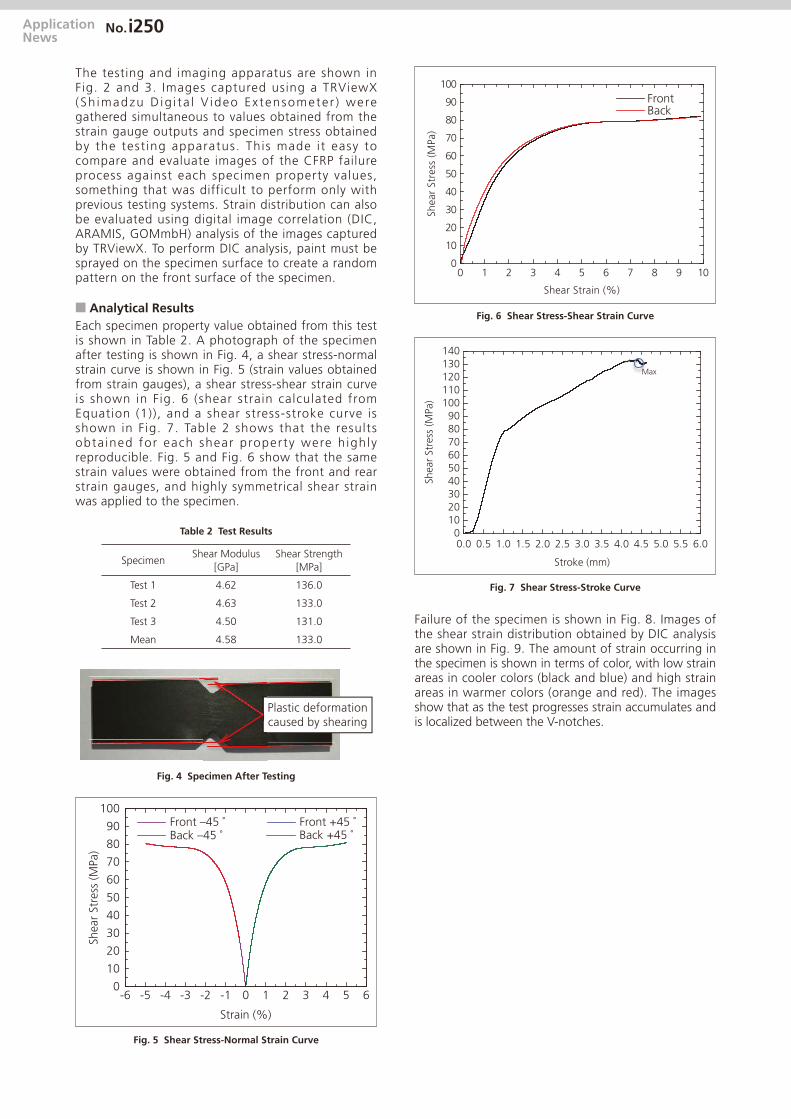
ApplicationNews
No.i250
The testing and imaging apparatus are shown in Fig. 2 and 3. Images captured using a TRViewX (Sh imadzu D ig i ta l V ideo Ex tensometer ) were gathered simultaneous to values obtained from the strain gauge outputs and specimen stress obtained by the test ing apparatus. This made it easy to compare and evaluate images of the CFRP failure process against each specimen property values, something that was difficult to perform only with previous testing systems. Strain distribution can also be evaluated using digital image correlation (DIC, ARAMIS, GOMmbH) analysis of the images captured by TRViewX. To perform DIC analysis, paint must be sprayed on the specimen surface to create a random pattern on the front surface of the specimen.
Analytical Results
Each specimen property value obtained from this test is shown in Table 2. A photograph of the specimen after testing is shown in Fig. 4, a shear stress-normal strain curve is shown in Fig. 5 (strain values obtained from strain gauges), a shear stress-shear strain curve is shown in Fig. 6 (shear strain calculated from Equation (1)), and a shear stress-stroke curve is shown in Fig. 7. Table 2 shows that the results obta ined for each shear property were h ighly reproducible. Fig. 5 and Fig. 6 show that the same strain values were obtained from the front and rear strain gauges, and highly symmetrical shear strain was applied to the specimen.
Table 2 Test Results
SpecimenShear Modulus
[GPa]
Shear Strength
[MPa]
Test 1 4.62 136.0
Test 2 4.63 133.0
Test 3 4.50 131.0
Mean 4.58 133.0
Plastic deformationcaused by shearing
Fig. 4 Specimen After Testing
-6 -5 -4 -3 -2 -1 0 1 2 3 4 5 60
10
20
30
40
50
60
70
80
90
100
Back +45 ˚Front +45 ˚
Back –45 ˚Front –45 ˚
Shear
Str
ess
(M
Pa)
Strain (%)
Fig. 5 Shear Stress-Normal Strain Curve
0 1 2 3 4 5 6 7 8 9 100
10
20
30
40
50
60
70
80
90
100
BackFront
Sh
ear
Str
ess
(M
Pa)
Shear Strain (%)
0.0 0.5 1.0 1.5 2.0 2.5 3.0 3.5 4.0 4.5 5.0 5.5 6.00
10
20
30
40
50
60
70
80
90
100
110
120
130
140
Sh
ear
Str
ess
(M
Pa)
Stroke (mm)
Max
Fig. 6 Shear Stress-Shear Strain Curve
Fig. 7 Shear Stress-Stroke Curve
Failure of the specimen is shown in Fig. 8. Images of the shear strain distribution obtained by DIC analysis are shown in Fig. 9. The amount of strain occurring in the specimen is shown in terms of color, with low strain areas in cooler colors (black and blue) and high strain areas in warmer colors (orange and red). The images show that as the test progresses strain accumulates and is localized between the V-notches.

ApplicationNews
No.i250
① ② ③ ④ ⑤Fig. 8 Specimen e Failure Process (images show the point at which the specimen fails)
① ② ③
④ ⑤ ⑥
⑦ ⑧ ⑨
Fig. 9 Shear Strain Distribution (DIC analysis images)

ApplicationNews
No.
© Shimadzu Corporation, 2016
For Research Use Only. Not for use in diagnostic procedure.
This publication may contain references to products that are not available in your country. Please contact us to check the availability of these
products in your country.
The content of this publication shall not be reproduced, altered or sold for any commercial purpose without the written approval of Shimadzu.
Company names, product/service names and logos used in this publication are trademarks and trade names of Shimadzu Corporation or its
affiliates, whether or not they are used with trademark symbol “TM” or “®”. Third-party trademarks and trade names may be used in this
publication to refer to either the entities or their products/services. Shimadzu disclaims any proprietary interest in trademarks and trade names
other than its own.
The information contained herein is provided to you "as is" without warranty of any kind including without limitation warranties as to its
accuracy or completeness. Shimadzu does not assume any responsibility or liability for any damage, whether direct or indirect, relating to the
use of this publication. This publication is based upon the information available to Shimadzu on or before the date of publication, and subject
to change without notice.
www.shimadzu.com/an/
i250
First Edition: Aug. 2016
Conclusion
We used this test system to successfully implement the V-notched beam method (ASTM D5379). In addition to evaluating the basic properties of shear modulus and shear strength, integrating a Digital Video Extensometer into the test system enabled us to capture reference data that can be used to elucidate the mechanism of failure of CFRP, allowing strain analysis to be performed in terms of specimen failure mode and DIC analysis.

ApplicationNews
No.i251
Material Testing System
Shear Test of Composite Material
(V-Notched Rail Shear)
LAAN-A-AG-E016
Introduction
Carbon fiber reinforced plastic (CFRP) do not oxidize or rust and have a higher specific strength and stiffness than existing materials. Applications of CFRP are being investigated, with a focus on applications as industrial products that require strength and durability. Compared to exist ing homogeneous materials, composite materials like CFRP are anisotropic, and display complex failure behaviors as a result of tension, compression, bending, in-plane shear, out-of-plane shear, or a combination of these stresses arising from loading in the principal-axis direction. In recent years, use of CAE analysis in industry has become widespread since it can reduce numbers of prototypes and reduce the cost of new product development. Because values for each of the stress properties stated above are needed to i n c rea se p re c i s i on when p red i c t i ng p roduc t characteristics during product design, there is a strong demand for test methods able to evaluate pure failure behaviors in CFRP.There are various tests methods for evaluating composite materials. Of these methods, two commonly used in-plane shear test methods to test in the direction of fibers in fiber reinforced composite materials and to test textile laminated materials are the Iosipescu method (ASTM D5379) that applies an asymmetrical four-point bending load to a specimen cut with notches, and method (ISO 14129) that applies a ±45˚ tensile load on laminated materials. We used the V-notched rail shear method (ASTM D7078) that can be used to test in-plane shear. Because this method uses a large gauge area on the specimen, it can accommodate specimens without holes and CRFP laminate materials that have discontinuous fibers.
Measurement System
The equipment configuration is shown in Table 1. Information on the specimen prescribed by ASTM D7078 is shown in F ig. 1. The specimen is a [0/90]10s orthogonally laminated material made from Toray T800S prepreg that was molded in an autoclave. The specimen has a 31-mm evaluation area (see Fig. 1), and two-axis strain gauges attached at the mid-point between the V-notches (center of evaluation area) that are able to measure strain in –45˚ and +45˚ directions. Shear strain can be calculated by inserting the strain values obtained from these two strain gauges into equation (1). Shear strain is a property needed to evaluate the shear modulus.
. Equation (1)
: Shear strain
: Strain at +45˚
+45 +=ε –45εγγ
+45ε: Strain at –45˚–45ε
In this test, strain gauges were attached on both the front and rear of the specimen. Calculating the mean of outputs obtained from strain gauges on both sides allows for more accurate measurement of the shear strain in the specimen, and confirms whether shear
strain is being applied symmetrically on the front and rear of the specimen.
Testing Machine : AG-50kNX plusLoad Cell : 50 kNTest Jig : ASTM D7078 jigSoftware : TRAPEZIUM X (Single)Test Speed : 2 mm/min
Table 1 Test Conditions
Strain gauge
90˚
31
.0
56
.0
76.0
in gaugen gaugin
9090
aiStra
Evaluation area
Fig. 1 Shape of Specimen
Fig. 2 Testing Apparatus
Fig. 3 Imaging Apparatus

ApplicationNews
No.i251
The testing and imaging apparatus are shown in Fig. 2 and Fig. 3. Images captured using a TRViewX (Shimadzu Digital Video Extensometer) were gathered simultaneous to values obtained from the strain gauge outputs and specimen stress obtained by the testing apparatus. This made it easy to compare and evaluate images of the CFRP failure process against each specimen property values, something that was difficult to perform only with previous testing systems. Strain distribution can also be evaluated using digital image correlation (DIC, ARAMIS, GOMmbH) analysis of the images captured by TRViewX. To perform DIC analysis, paint must be sprayed on the specimen surface to create a random pattern on the front surface of the specimen.
Analytical Results
Each specimen property value obtained from this test is shown in Table 2. A photograph of the specimen after testing is shown in Fig. 4, a shear stress-normal strain curve is shown in Fig. 5 (strain values obtained from strain gauges), a shear stress-shear strain curve is shown in Fig. 6 (shear strain calculated from Equation (1)), and a shear stress-stroke curve is shown in Fig. 7. Table 2 shows that the results obta ined for each shear property were h ighly reproducible. Fig. 5 and Fig. 6 show that the same strain values were obtained from the front and rear strain gauges, and highly symmetrical shear strain was applied to the specimen.
Table 2 Test Results
Specimen Shear Modulus
[GPa]
Shear Strength
[MPa]
Test 1 4.63 121.72
Test 2 4.55 120.00
Test 3 4.58 120.05
Mean 4.59 120.60
Plastic deformationcaused by shearingPcc
Fig. 4 Specimen After Testing
-6 -5 -4 -3 -2 -1 0 1 2 3 4 5 6
10
20
30
40
50
60
70
80
90
100
Back +45˚Front +45˚
Back –45˚Front –45˚
Strain (%)
Sh
ear
Str
ess
(M
Pa)
0
Fig. 5 Shear Stress-Normal Strain Curve
0 1 2 3 4 5 6 7 8 9 100
10
20
30
40
50
60
70
80
90
100
BackFront
Sh
ear
Str
ess
(M
Pa)
Shear Strain (%)
Fig. 6 Shear Stress-Shear Strain Curve
0.0 0.5 1.0 1.5 2.0 2.5 3.0 3.5 4.0 4.5 5.0 5.5 6.00
10
20
30
40
50
60
70
80
90
100
110
120
130
140
Sh
ear
Str
ess
(M
Pa)
Stroke (mm)
Max
Fig. 7 Shear Stress-Stroke Curve
Failure of the specimen is shown in Fig. 8. A crack that appears c lose to the upper notch quickly propagates down toward the bottom notch during a simultaneous decrease in test force. Images of the shear strain distribution obtained by DIC analysis are shown in Fig. 9. The amount of strain occurring in the specimen is shown in terms of color, with low strain areas in cooler colors (black and blue) and high strain areas in warmer colors (orange and red). The images show that as the test progresses strain accumulates and is localized between the V-notches.
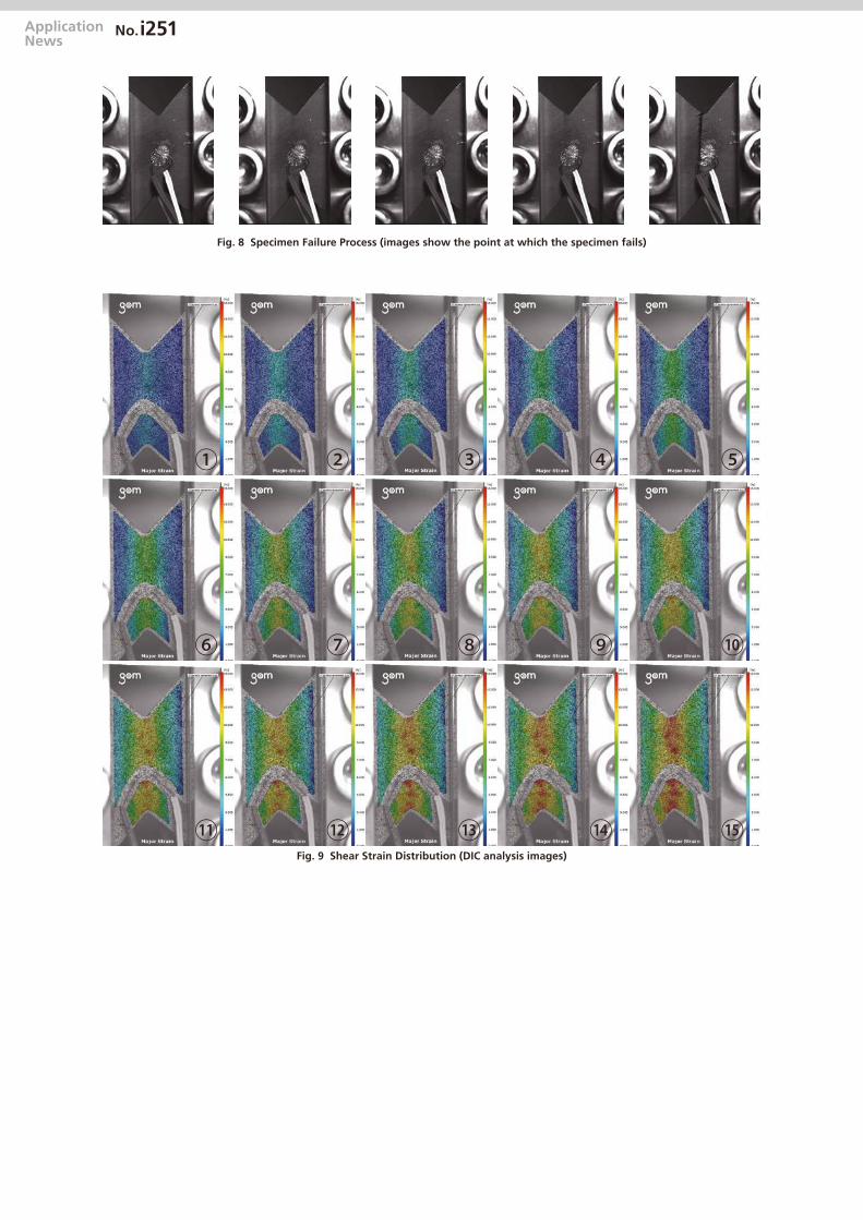
ApplicationNews
No.i251
Fig. 8 Specimen Failure Process (images show the point at which the specimen fails)
① ② ③ ④ ⑤
⑥ ⑦ ⑧ ⑨ ⑩
⑪ ⑫ ⑬ ⑭ ⑮Fig. 9 Shear Strain Distribution (DIC analysis images)

ApplicationNews
No.
© Shimadzu Corporation, 2016
For Research Use Only. Not for use in diagnostic procedure.
This publication may contain references to products that are not available in your country. Please contact us to check the availability of these
products in your country.
The content of this publication shall not be reproduced, altered or sold for any commercial purpose without the written approval of Shimadzu.
Company names, product/service names and logos used in this publication are trademarks and trade names of Shimadzu Corporation or its
affiliates, whether or not they are used with trademark symbol “TM” or “®”. Third-party trademarks and trade names may be used in this
publication to refer to either the entities or their products/services. Shimadzu disclaims any proprietary interest in trademarks and trade names
other than its own.
The information contained herein is provided to you "as is" without warranty of any kind including without limitation warranties as to its
accuracy or completeness. Shimadzu does not assume any responsibility or liability for any damage, whether direct or indirect, relating to the
use of this publication. This publication is based upon the information available to Shimadzu on or before the date of publication, and subject
to change without notice.
www.shimadzu.com/an/
i251
First Edition: Aug. 2016
Conclusion
We used this test system to successfully implement the V-notched rail shear method (ASTM D7078). In addition to evaluating the basic properties of shear modulus and shear strength, integrating a Digital Video Extensometer into the test system enabled us to capture reference data that can be used to elucidate the mechanism of failure of CFRP, allowing strain analysis to be performed in terms of specimen failure mode and DIC analysis.

■ Introduction As the result of recent progress of research and development, carbon fiber materials have been put to practical use in a wide range of implements, including space aircraft parts, sporting goods like golf club shafts and tennis rackets, structure materials that must transmit X-rays, and acoustic materials. A group of high-quality carbon fibers is further classified, according to its tensile strength, into several groups. One of these is a high-strength fiber group that features in excellent tensile strength; another is a high-elasticity fiber group characterized by high flexibility, but with a tensile strength of no more than around 2,000 MPa. As described above, data on mechanical properties are indispensable information for classifying fibers. The following is an example of tests for evaluation of physical behaviors under a compressive force applied to carbon fibers (single fibers) having different tensile strength levels with Shimadzu Micro Compression Testing Machine MCT.
■ Testing Conditions (1) Testing mode: compression test (2) Testing load: 200 gf (3) Loading rate constant: 1 (4,230 gf/sec.) (4) Calculation of strength: Compression strength is calculated by the following equation. *1
𝑆𝑆𝑆𝑆𝑆𝑆𝑆𝑆 = 2 ∙ 𝑃𝑃𝑃𝑃 ∙ 𝜋𝜋𝜋𝜋 ∙ 𝑑𝑑𝑑𝑑 ∙ 𝐿𝐿𝐿𝐿
where: ST: tensile strength (kg/mm2) P: compression strength (kgf) d: diameter of fiber (mm) L: length of fiber (mm) Note *1: from JIS A1113-1976 Method of tests for splitting tensile strength of concrete
Material Testing System MCT
Compression-Rupture Test of Carbon Fibers with Different Tensile Characteristics Shimadzu Micro Compression Testing
No. SCA_300_037

■ Test Piece (1) Name: Carbon fibers (PAN type
carbon fibers)
(2) Types: 1 (high-ductility type)
2 (high-strength type)
3 (ultra-high elasticity type)
(3) Shape: See Fig. 1
Fig. 1 A Microscopic photograph of Test Piece before Test
Fig. 2 A Microscopic photograph of Test Piece after Test
Fig. 3 Load- Deformation Curves of High Ductility Samples
Fig. 4 Load- Deformation Curves of High Ductility Samples
Fig. 5 Load- Deformation Curves of High Ductility Samples
No. SCA_300_037

Type of test piece Compression-rupture strength(kgf/mm2)
Standard deviation (kgf/mm2)
High-ductility type 149.90 3.23 High-strength type 151.09 6.34 Ultra-high elasticity type 68.87 4.37
Table 1 Results of Compression-Rupture Test of Carbon Fibers
Note: The length of the indenter diameter (50 mm) was used for the length of fiber because the test piece was extraordinarily long.
■ Test Results Table 1 shows a summary of test data, and Figs. 2-4 show the compression-rupture strength and the overlapping view of load-deformation curves for each test piece. The difference of behavior between test pieces are observable in the load-deformation curves of Figs. 2-4. The test pieces of the high-ductility type and the high-strength type have similar compression-rupture strength, while the ultra-high elasticity type has a remarkably low compression-rupture strength. (Refer to Table 1) Admitting some deviation among the test data as a result of the surface conditions of the test pieces, the test results ensure that this testing machine is useful and effective for evaluation of mechanical properties of single fibers, provided that data are processed statistically. * Please be advised that data obtained before the implementation of the current Weights and Measures Law may be presented in terms of gravimetric unit.
No. SCA_300_037

■ Introduction Most mass produced molded plastic products are injection-molded. The appropriate temperature and pressure for injection molding differs depending on the type of resin and shape of the die, over-filling, under-filling, sink marks, voids, or other molding defects. Even if appropriate molding parameters are used, any changes in the status of the resin raw materials used could cause molding defects as well. Therefore, it control the quality of resin raw materials on a daily basis. Furthermore, it is important to perform the daily resin high pressure conditions that approximate molding conditions, which is not possible using the melt flowrate measurement method.
■ Viscosity Evaluation Using Constant Temperature Method Polycarbonate (PC) samples of various molecular weights containing 33 % glass fiber (GF) were measured using constant temperature method. The flow curves clearly show that the higher the molecular weight, the higher the sample’s viscosity.
Test Method Constant temperature test
Die Diameter 1 mm
Die Length 10 mm
Test Temperature 280 ℃
Test Pressure 1.96 MPa
Preheating Time 300 sec
Sample Size 1.5 g Test Conditions
Test result
Material Testing System CFT
Viscosity Evaluation of Thermoplastic Resins (GFRP) No. SCA_300_055

Sample No. Component Molecular Weight GF Ratio (%) Shear Rate (S-1)
Viscosity (Pa•s)
1 PC/SGF 17000 33 44,7 1,098 2 PC/SGF 22000 33 30,6 1,604 3 PC/SGF 26000 33 18,5 2,657
Test Results
■ Selection of Measurement Method According to Material Constant Temperature Method In the testing method based on the use of a constant temperature, two calculation points on the piston's descent are set beforehand. The calculation is conducted using either the limiting method or the automatic method. In the limiting method, the flowrate is determined from the stroke-time curve of the piston between the above two points. In the automatic method, the stroke-time curve is divided into 20 segments, and the flowrate is determined from the gradients of the curves of those segments except for the first and last segment, with the maximum value taken automatically as the flowrate.
No. SCA_300_055

Most mass produced molded plastic products are injection-molded. The appropriate temperature and pressure for injection molding differs depending on the type of resin and shape of the die, over-filling, under-filling, sink marks, voids, or other molding defects. Even if appropriate molding parameters are used, any changes in the status of the resin raw materials used could cause molding defects as well. Therefore, it control the quality of resin raw materials on a daily basis. Furthermore, it is important to perform the daily resin high pressure conditions that approximate molding conditions, which is not possible using the melt flowrate measurement method.
■ Changes in Viscosity Due to Moisture Absorption Time The change in resin viscosity due to moisture absorption was measured using sample (1), with a molecular weight of 17,000. After drying for 13 hours in a vacuum environment at 100 °C, the sample was left in a room with a temperature of about 23 °C and about 50 % relative humidity for constant temperature testing. The graph shows that the fluidity increases and viscosity decreases as more moisture is absorbed. The results show that about 4 hours after leaving the sample there, viscosity drops sharply and then almost stops decreasing after about 24 hours. Due to the large changes in resin viscosity that result from moisture absorption, using resin materials that have not been controlled for moisture can result in injection molding failures.
Therefore, such injection molding problems can be avoided by using a CFT-EX series flowtester to measure the viscosity to ensure that it iswithin given standards before molding the parts.
Test Results
Material Testing System CFT
Viscosity Evaluation of Thermoplastic Resins (GFRP)
No. SCA_300_056

Conditioning Time(H)
Share Rate (s-1)
Viscosity (Pa・s)
0 44,38 1,105 0,25 46,84 1,047 0,5 47,35 1,036 1 47,38 1,035 2 50,41 973 4 53,03 925 8 55,54 883 24 58,77 834 48 58,61 837
Test Results
■ Selection of Measurement Method According to Material Constant Temperature Method In the testing method based on the use of a constant temperature, two calculation points on the piston's descent are set beforehand. The calculation is conducted using either the limiting method or the automatic method. In the limiting method, the flowrate is determined from the stroke-time curve of the piston between the above two points. In the automatic method, the stroke-time curve is divided into 20 segments, and the flowrate is determined from the gradients of the curves of those segments except for the first and last segment, with the maximum value taken automatically as the flowrate.
■ CFT-EX Series
No. SCA_300_056

CFRP (carbon fiber reinforced plastic) has attracted attention as a high-performance composite material with high strength and rigidity, yet low in weight, and is being applied in various fields, such as for aircraft, railroad vehicles, automobiles and civil engineering. This example describes evaluating the characteristics of a flat plate specimen of CFRP material when a tensile load is applied (tensile test) and observing the fracture status. Tensile testing consisted of static testing of material strength and measuring the modulus of elasticity using a precision universal testing machine. In addition, high-rate tensile impact test was also performed. In the latter case, a high-speed video camera was used to record specimen fracture, which allowed capturing image data of the instant the CFRP material fractured. ■ Test specimen The tensile test specimen tested in this example is shown in figure 1. Included 50 mm long CFRP tabs attached to both ends of the CFRP strip with thermosetting resin adhesive. Reinforcing the grip area with tabs ensures a stable tensile test with good reproducibility.
Figure 1: CFRP test specimen
Specimen details are as follows: 1) Material: unidirectional CFRP 2) Shape: strip (with tabs on both ends) 3) Specimen dimensions: for static tensile
testing 200(L) x 12.5(W) x 1(T) mm. For recording image of impact fracture 70(L) x 6.25(W) x 0.3(T) mm
■ Static tensile test A strain gauge type extensometer was attached to the specimen and a tensile test was performed using a precision testing machine. The extensometer was removed when strain exceeded the elasticity measurement range. It is also possible to measure strain by affixing a strain gauge instead of an extensometer. Tensile test parameters are indicated below. (1) Tensile rate: 10 mm/min (2) Grip distance: 100 mm (3) Test force detection: 50 KN load cell (4) Extensometer gauge length: 50 mm (5) Elasticity calculation range: 5/10,000 to
25/10,000 strain
Figure 2: Static test results
Material Testing System AG-X
Observation of fracture in CFRP tensile test
No. SCA_300_059

The elasticity of CFRP specimen can be determined by calculating the slope of the given strain region (elasticity calculation range) in the stress-strain curve (figure 2) obtained from test results. Tensile strangth can be determined from the maximum stress in the stress-displacement curve (figure 3) before the specimen breaks.
Figure 3: Static test results
The following values were obtained from the measurement data. (1) Tensile strength: 346 GPa (2) Elasticity: 148 GPa
The post-test status of the specimen is shown in figure 4. Compared to the starting status in figure 1, it clearly shows how the fibers within the resin have failed.
Figure 4: Specimen status after static test
■ Static tensile test To verify functionality, development of composite materials involves not only static Static strength testing, but also involves the objective of ensuring active safety. Consequently, it is important to determine the shock strength and understand the process of fracture propagation. Therefore, the fracture process during tensile chock testing of a CFRP specimen was observed by combining a high-speed video camera with high-rate tensile shock test machine. Observation conditions are indicated below. Specimen tensile rate: 6 m/s
Grip distance: 30 mm
Camera lens: 105 mm macro, with 2 x teleconverter
Camera lighting: strobe
Camera trigger:
signal synchronized with tensile displacement is sent from testing machine to camera.
The setup used to record video of the test is shown in figure 5, with a high-speed video camera mounted about 450 mm in front of the specimen. Recording was activated by an external start trigger signal sent from the testing machine to the camera, which was synchronized to the tensile displacement. A strobe light synchronized to the video timing was used as lighting.
Figure 5: Setup of high-rate shock test
No. SCA_300_059

Using this test configuration, a load was applied to the CFRP specimen according to the parameters indicated above and a high-speed camera captured the instant of fracture, at 250.000 frames per second. This image data shown in figure 6. This shows 8 consecutive frames, from (1) TO (8), with an interval of 4 microseconds between each frame. This camera features highly detailed image resolution of 312
horizontal by 260 vertical pixels that is constant, regardless of the frame rate. This example shows, combining a high-speed video camera and material testing machine makes it possible to evaluate material properties and observe fracture behavior at the same time. This enables supporting a wide range of material development applications, from developing individual functionally enhanced resins to developing composite materials.
Figure 6: Images of specimen during fracture
No. SCA_300_059

5. Food Industry

1st characteristic
2nd characteristic General Term Characteristic content
Hardness Soft / teeth resistance / hard
Required force for even deformation and internal binding power providing food product shape
Cohesive quality
Brittleness Crumbly / Munchy / Brittle
Related to the force, hardness and cohesive quality when chewing a food product
Masticable quality
Soft / tough Relation between energy, hardness, cohesive quality and elastic quality required for mastication up to the point of swallowing a compressed food product
Gum quality Easy loss of shape / powder state / paste state / rubber state
Relation between energy, hardness and cohesive quality, required for mastication up to the point of swallowing a semi-compressed food product
Cohesiveness Dry / cohesive Degree of fluidity at force for displacement
Elastic quality Plasticity / elasticity Rate at which food that is deformed by an external force but returns to original shape after external force is released
Adhesiveness Glutinous / adhesiveness / stickiness
The force required to overcome traction between the surface of a food product and items such as tongue teeth, and palate
Szczesniak Texture Profile AnalysisMechanical characteristics
5. Food Industry
CONSISTENT QUALITY FOR THE RIGHT LOOK, FEEL, SHAPE AND TASTE
Food & beverages are very emotional products: although people either like or dislike certain products, food is in general associated with fun and enjoyment, with culture, style and way-of life. A further psychological aspect around food: we give food access into our bodies.
To stimulate consumption on a regular basis, food products also have to have a consistent quality regarding the right look, feel, shape and taste. Food designers, manufacturers and processors are aware of these challenges, particularly when handling natural products.
Today, food and beverages production is run and controlled by advanced technologies. They are used for natural, agricultural
and meat products, but also for food and beverages which have been mixed in laboratories or production plants.
Food texture is the sense of touch when food is handled, the visual sense recorded by eye and oral touch sensation and palatability. Food products are tested for their mechanical characteristics, hardness, cohesive and elastic qualities as well as adhesiveness.
Whether butter, margarine, agar, pork, jelly bears or pickled plums – please see the multitude of applications on the following pages.

5. Food Industry
No.i246 Texture evaluation of care food
No.11 Evaluation of foods for people with dysphagia
No.21 Compression tests of microcapsules containing aroma components
No.12 evaluation of food texture
SCA_300_003 An application of Shimadzu flowtester model CFT to food products
SCA_300_004 An evaluation of viscosity of non-vulcanized rubber by Shimadzu flow tester
SCA_300_005 Cereal compression shear test evaluation of food
SCA_300_006 Chewing properties of gummy bears test
SCA_300_015 Evaluation of texture using a multi-piercing jig evaluation of food
SCA_300_016 Evaluation test of butter and margarine evaluation of foods
SCA_300_027 Measurement of texture characteristics of rice using title line the EZ test Shimadzu texture analyzer
SCA_300_032 Texture evaluation of cheese and agar jelly
SCA_300_042 Evaluation test of foods for people with difficulty swallowing
SCA_300_046 Measurement of texture of pork by a penetrating strength test
SCA_300_048 Multifaceted measurement of plums pickled in plum wine
SCA_300_051 Texture analysis of “soumen” japanese vermicelli
SCA_300_052 Texture analysis of ikura salted
SCA_300_053 Texture evaluation of cheese and agar jelly

ApplicationNews
No.
LAAN-A-AG-E011
Material Testing System
Texture Evaluation of Care Food
i246The development of care food, which is processed to be soft and easy to eat, is steadily progressing to the point t h a t t h e s h a p e , c o l o r a n d t a s t e a r e n e a r l y indistinguishable from ordinary food, except that the texture is softened to enable crushing using just the gums and tongue. These commercially available products are a great boon to the elderly and individuals with internal mouth injuries who may have inadequate strength for chewing and drinking, and are helping these disadvantaged groups to better enjoy the pleasures of tasting and eating. Meanwhile, according to the Health Promotion Law in Japan, the Japan
Consumer Affairs Agency is authorized to conduct reviews of the suitability of "foods for people with dysphagia" as regulated special purpose foods, and based on these reviews, permit the display of such foods. Here, we conducted measurements of commercially available care food based on the test methods specified for reviewing the suitability of foods for people with dysphagia. We then classified the food according to the specific standard based on the obtained hardness, adhesiveness, and cohesiveness data.
n Introduction
The instrument used for this evaluation was the Shimadzu EZ Test Texture Analyzer, with a 5N test force measurement load cell. The samples used consisted of 3
commercially available care food products (sample names: A – C).
n Testing Equipment and Specimens
An overview of the measurement setup is shown in Fig. 1. The sample diameter was 40 mm, and the sample was loaded to a height of 15 mm in the 20 mm high sample container. Using a plastic plunger 20 mm
in diameter and 8 mm in height, compression testing was conducted twice at a speed of 10 mm/sec with a clearance of 5 mm. The test was conducted using a sample temperature of 20 °C.
n Test Conditions
The results obtained from testing of 3 types of food products are shown in the force – time graphs of Fig. 2 – Fig. 4. n Test Results
Fig. 1 Overview of Texture Test Fig. 2 Food A (vegetable soup)
-0.4
-0.2
0.0
0.2
0.4
0.6
0.8
1.0
Time (sec)0 1 2 3 4 5
Forc
e (N
)

For Research Use Only. Not for use in diagnostic procedures.The contents of this publication are provided to you “as is” without warranty of any kind, and are subject to change without notice. Shimadzu does not assume any responsibility or liability for any damage, whether direct or indirect, relating to the use of this publication.
First Edition: January, 2012
www.shimadzu.com/an/ © Shimadzu Corporation, 2012
Table 1
SampleHardness Adhesiveness Cohesiveness Permissible Standard
(Overall Judgment)Measured Value (N/m2) Judgment Measured Value (J/m3) Judgment Measured Value Judgment
Food A 0.84 × 10³ Ⅰ, Ⅱ, Ⅲ 0.19 × 10³ Ⅰ, Ⅱ, Ⅲ 0.82 Ⅰ, Ⅱ Ⅲ
Food B 1.97 × 10³ Ⅰ, Ⅱ, Ⅲ 0.41 × 10³ Ⅰ, Ⅱ, Ⅲ 0.76 Ⅰ, Ⅱ Ⅲ
Food C 1.88 × 10³ Ⅰ, Ⅱ, Ⅲ 0.08 × 10³ Ⅰ, Ⅱ, Ⅲ 0.52 Ⅰ, Ⅱ Ⅲ
The results obtained from the series of measurements are shown in Table 1.
The measured values for hardness, adhesiveness and cohes iveness that are within the range of the permissible standard are indicated with a that surrounds the standards in the Judgment field. Food A does not satisfy the hardness standards Ⅰ andⅡ, so the permissible standard was designated as Ⅲ. In the case of foods B and C, item Ⅰ is not satisfied, so the
permissible standard would be presumed to be Ⅱ. However, the permissible standard becomes Ⅲ in the final evaluation, because food B and food C contain non-homogeneous ingredients. Thus, by defining the numerical value and comparing it with the judgment standards, the judgment can be made as to which permissible standard it corresponds.
[Reference](Permissible Standards of Foods for People with Dysphagia Note 1))Note 1) Regarding permission to display special usage foods (Excerpted from Ministry of Health, Labour and Welfare Food Safety Notification
No. 0212001)
Standard*1 Permissible StandardⅠ*2 Permissible StandardⅡ*3 Permissible StandardⅢ *4
Hardness (Resistance during compression at constant rate) (N/m2)
2.5 × 10³ - 1 × 10⁴ 1 × 10³ - 1.5 × 10⁴ 3 × 10² - 2 × 10⁴
Adhesiveness (J/m3) 4 × 10² or less 1 × 10³ or less 1.5 × 10³ or less
Cohesiveness 0.2 - 0.6 0.2 - 0.9 -
*1 Within the permissible range of the standard under conditions of either of ambient temperature or the normal temperature at which eating takes place.
*2 Homogeneous items (for example, jellied foods)*3 Homogeneous items (for example, jellied or smooth foods). However, this excludes foods that satisfy permissible standard Ⅰ.*4 Includes non-homogeneous foods (for example, rice gruel which is easily clumped or collected, soft paste-like or jellied foods).
However, this excludes foods that satisfy permissible standard Ⅰ or permissible standard Ⅱ.
Fig. 3 Food B (rice gruel) Fig. 4 F ood C (sukiyaki)
-0.4
-0.2
0.0
0.2
0.4
0.6
0.8
1.0
Time (sec)0 1 2 3 4 5
Forc
e (N
)
-0.4
-0.2
0.0
0.2
0.4
0.6
0.8
1.0
Time (sec)0 1 2 3 4 5
Forc
e (N
)

° ± ° ° ± °° ±°° ± °
φ
φ
°
× ×
× × × ×
時間
試験
力
時間
試験
力


21
LAAN-J-E-HN01
Material Testing & Inspection
Micro Compression Testing Machine
Measurement Results
Introduction
Recently, some washing agents include microcapsules containing aroma components, in order to sustain the smell of clothes after washing. The diameter of these microcapsules is in the order of several tens of m, and when the appropriate pressure or friction is applied, the beads burst open and the fragrance is released. This Application Data Sheet describes compression tests carried out on microcapsules containing aroma components using an MCT Series Micro Compression Testing Machine. F Yano
Item Set Value
Test speed Indenter
3.87 mN/sFlat indententer 120 m dia.
Table 1 Test Conditions
Measurement and Jigs
The diameters of the microcapsule particles measured with an optical microscope were about 10 to 20 m, and a flat indenter with a tip diameter of 120 m was used as the upper pressure indenter. Table 1 shows the test conditions.
Fig.1 Photograph Taken Using a Microscope
Microcapsule
Test Force at Break Displacement at Break Particle Diameter
1.57 mN 0.96 m 9.01 m
Fig. 2 Test Results
Test
forc
e (N
)
10.0
0
0 2 Displacement (m)
Compression Tests of MicrocapsulesContaining Aroma Components
Break
Table 2 Bead Compression Testing Results

21
First Edition: February 2013
© Shimadzu Corporation, 2013www.shimadzu.com/an/
Shimadzu Corporation
Microcapsule Compression Test System
Features
MCT Micro Compression Testing Machine
Measurement of Minute Compression DisplacementsIn order to evaluate the compression properties of minute test specimens, two types of testers with different measurement ranges are provided, for measurements up to 100 m with a resolution of 0.001 m, and for measurements up to 10 m and resolution of 0.0001 m.
Wide Loading RangeIn order to compress minute test specimens, two types are provided with maximum forces of 4903 mN and 1961 mN respectively.
High Accuracy MeasurementsThe accuracy of measurement is within 1 % of the set or displayed test force, whichever is greater.
Sample Size Measurement Function Provided as StandardThe sample size measurement function using an overhead image is provided as standard. It allows determination of the geometric mean diameter, length, etc.
Length Measurement on PC Screen and Saving of Images (optional)Use the length measurement kit (color or monochrome) to display the overhead image on the PC screen to measure the length of the sample. The image can be saved as digital data.
Display of Sample Images During Compression (optional)Images captured in side observation during compression can be displayed (the optional side observation kit is required).
Testing Possible under High-Temperature Conditions (optional)Testing can be performed in temperature conditions ranging from 50 to 250 C.
Tester: MCT
Indenter: Truncated cone flat indenter (dia.: 120 m)
Length measurement Length measurement kit
Side observation: Side observation kit

φ
φ
×
× ×
°
時間
試験
力
××
×
×
××


Shimadzu Flowtester Model CFT, usually used for testing the flow of high polymer materials for data of their flowability properties - viscosity and softening - or for determination of their forming process conditions, is expanding its application to the field of food testing as well. The following is an introduction of the result of flow tests on three different types of rice cakes available on the market.
■ Flowability properties of viscosity and softening were measured with a constant rate heating method on three types of rice cake paste; two of them pounded manually with a cooking pestle, and the other by a mixing machine
■ Test conditions:
Specimens:
(1) Rice cake A by cooking pestle, much moisture
(2) Rice cake B by cooking pestle, little moisture
(3) Rice cake C by mixing machine
Test temperature:
initial temperature 40 °C (preheated for 180 sec.)
heated thereafter at constant rate of 2 °C/min.
Extruding conditions
:
extruding pressure: 10 kgf/cm2,
Die: D1 x 1 mm (diam. x length)
Testing machine
:
Shimadzu Flowtester Model CFT
Material Testing System CFT
An Application of Shimadzu Flowtester Model CFT to Food Products Measurement of stickiness and flowability of rice cake paste Model CFT to Food Products No. SCA_300_003

■ Softening - flowability characteristic curves
As shown in Fig.1, the softening - fluidifying process is presented in relation to temperature. The three cakes were softened at the ascending temperature in the order of cake A, cake C and cake B.
Fig. 1 Softening- Flowability Characteristic Curves
Note: The piston stroke in Fig.1 is equivalent to the quantity of specimen extruded (stroke of 1 mm = 0.1 ml).
* Please be advised that data obtained before the implementation of the current Weights and Measures Law may be presented in terms of gravimetric unit.
No. SCA_300_003

■ Introduction In general, rubber for industrial use are processed through vulcanization in order to meet various requirements in hardness or elasticity (viscosity). Rubber is usually evaluated by Mooney Viscometers at the vulcanization process, but it can also be tested by Flow Testers to obtain useful information of its viscosity as well. The following sections are dedicated to reporting comparison and evaluation of the test result on three kinds of non-vulcanized rubber, using a Mooney viscometer and a Shimadzu Flow Tester. Table 1 shows the test result by the Mooney Viscometer. Test parameters are: test temperature 100 °C, pre-heating time 1 min., test time 4 min. and rotor type L.
Sample Code ML 1+4(100 °C)
Sample 1 83 Sample 2 78 Sample 3 73
Table 1: Measured Mooney viscosity value The same samples were measured by the Shimadzu Flow Tester of constant load (pressure) extrusion capillary rheometer type, with the following result.
Material Testing System CFT
An evaluation of viscosity of non-vulcanized rubber by Shimadzu flow Tester
No. SCA_300_004

Fig. 1: Viscosity – Temperature Curve
Fig.1 shows the result of tests with the extruding pressure (load) of 3.432 MPa (35 kgf) and at the temperature of three different steps of 90.0 °C, 110 °C, and 130 °C. In the lower temperature range, difference between the three samples is clearly observed. Sample 1 has the highest viscosity followed by Sample 2 and sample 3 in Mooney viscosity. This order in terms of Mooney viscosity, however, is upset between sample 1 and sample 2 in the test result by the Shimadzu Flow Tester. At 130 °C however, the three samples are in the same order between the Mooney viscosity tester and the Shimadzu Flow tester. This fact indicates that the sample 2 has a nature of being vulnerable to thermal influence on its viscosity fluctuation. Another test was exercised with different extruding pressures (loads) in an effort of searching further difference among the three samples. The result is shown in Fig.2.
Fig. 2 Viscosity – shearing speed curve
Tests were performed with the test temperature of 90 °C and three different extruding pressures of 3.432 MPa (35 kgf), 4.903 MPa (50 kgf), and 6.865 MPa (70 kgf). The test result rearranged in terms of shearing speed are shown in Fig. 2. Traverse speed accounts for the flowing out speed of sample, which is one of the important factors for the engineering process including extruder forming. It is observed from Fig. 2 that the difference in shearing speed does not cause such an obvious difference as observed in the difference of temperature. The curves show a trend similar to that of Fig. 1 in the low extruding pressure (low shearing speed) range, while the order of the curves for sample 1 and 3 is upset each other in the high extruding pressure (high shearing speed) range. This is another trend different from that of Mooney viscosity. The curves of Fig. 2 also indicates that viscosity of sample 3 is less influenced by extruding pressure than the other two samples. As seen above, tests with different apparatus having different evaluation tolls will provide an opportunity for reviewing from a different angle. Shimadzu flow tester, which is a viscosity evaluation equipment for plastics in general, is also useful in viscosity evaluation of other various materials as it permits a wide range of test parameter choice. Materials, like rubber, for instance, which is hard and has high viscosity, can well be evaluated with a larger die (nozzle). The above data were obtained by use of a die with hole dia. of 3 mm and die length of 3 mm. * Please be advised that data obtained before the implementation of the current Weights and Measures Law may be presented in terms of gravimetric unit.
No. SCA_300_004

■ Introduction The following describes using a specialized Kramer shear cell jig to measure the hardness of breakfast cereal. The overall hardness and crunchiness of the cereal can be evaluated based on the initial slope of the test force curve and the jaggedness of the curve that results from individual cereal pieces breaking.
When evaluating samples that have nonuniform shapes, non-uniform internal characteristics, or include a mixture of various kinds of substances, it can be difficult to interpret meaning from the resulting graph and to obtain reproducible data. This is caused by the influence the testing location and characteristics of individual samples
have on the data. To minimize such effects, multiple blades are used to perform compression shear tests. By using multiple blades, the resulting test force curve indicates the total test force for multiple blades, allows obtaining reproducible data.
Compression Shear Test of Cereal Results from Compression Shear Test of Cereal Using Kramer Shear Cell Jig
Material Testing System EZ-Test
Cereal Compression Shear Test Evaluation of Foods No. SCA SCASCA_300_005
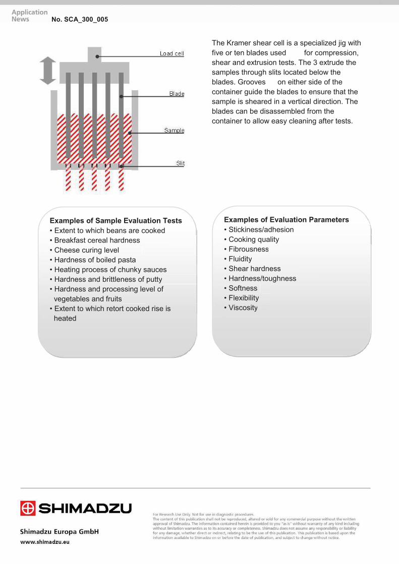
The Kramer shear cell is a specialized jig with five or ten blades used for compression, shear and extrusion tests. The 3 extrude the samples through slits located below the blades. Grooves on either side of the container guide the blades to ensure that the sample is sheared in a vertical direction. The blades can be disassembled from the container to allow easy cleaning after tests.
Examples of Sample Evaluation Tests • Extent to which beans are cooked • Breakfast cereal hardness • Cheese curing level • Hardness of boiled pasta • Heating process of chunky sauces • Hardness and brittleness of putty • Hardness and processing level of • Hardness and processing level of vegetables and fruits • Extent to which retort cooked rise is heated
Examples of Evaluation Parameters • Stickiness/adhesion • Cooking quality • Fibrousness • Fluidity • S hear hardness • Hardness/toughness • Softness • Flexibility • Viscosity • Viscosity
No. SCA_300_005

■ Purpose and Definition Food texture is a very important characteristic when we eat. We want our meal or snack to be crispy, soft, creamy, crunchy, sticky, hard and so on. Another important reason to test texture is production efficiency. The testing of chewing properties of, for example gummy bears, is important to make production time as short as possible. By testing chewing properties the producer can optimize the time the gummy sweets need to stay in a stove oven during production, hereby optimizing production time, and produce a product with consistent quality and properties. ■ Equipment used: Testing machine: EZ-LX or SX/ AGS-XTable top
Load cell: 200N,1/500 Class1
Jig: Compression plate
Software: TrapeziumX, Texture / Compression
Environment: Room temp. 21 °C, +/-2 °C, humidity appr. 50 +/-5% RH.
Fig.1 EZ-SX
■ Test Jig The jigs used were the standard lower Ø 100 mm compression plate, 343-08095, (346-51687-12 can also be used) and the Tooth pushrod A. (346-52258-02).
Fig.2 Test Jig
Material Testing System EZ-X
Chewing properties of gummy bears test No. SCA_300_006

■ Test execution:
Five samples were tested where we are looking for elastic properties as well as adhesive and hardness properties. These are all factors which affects the chewing properties of a gummy sweet. A method is prepared as described under “Creating a chewing test method” in the help section of the TrapeziumX software. Test type is Texture and compression. Test speed is set to 50 mm/min and the test is performed by doing two compressions to 6 mm in this case with a return to 0 mm between each compression. It is necessary to completely off-load the sample to get the negative force from the stickiness, which gives the adhesive properties of the sample. TrapeziumX is already prepared for this test so the method description can be found in the help section including how to prepare the calculations needed in the calculator of TrapeziumX.
Fig.3 Test Setup
Fig.4 Test Method
Fig. 5 Test Definition
No. SCA_300_006

■ Test Results: By testing chewing properties the producer can optimize the time the gummy sweets need to stay in a stove oven during production, hereby optimizing production time, and produce a product with consistent quality and properties. The Texture module of the Trapezium software provides pre-defined data points for this type of tests and for the chewing properties test we used the guideline in the Trapezium help section. Some of the results presented are hardness, elastic properties, cohesiveness and adhesiveness. HARDNESS is the force required to compress the sample to a pre-defined point.
ELASTICITY is the rate with which a deformed sample returns to its original length/size after deformation.
COHESIVENESS is the strength of the internal bonds making up the body of the product. (Greater the value the greater the cohesiveness). ADHESIVENESS is the work necessary to overcome the adhesive forces between the surface of the sample and the surface of other materials with which the sample comes into contact with. Force required to pull food away from surface. All together important properties of a gummy candy and the base for the texture experience we all expect when putting that wine gum or gummy bear in to our mouths.
Fig. 6 Test Results
Fig. 7 Test Results
No. SCA_300_006

■ Introduction Piercing tests are often used to evaluate food texture. Due to air bubbles, hard particles, or other variations in the internal structure of samples, however, test results can vary depending on where the sample is pierced, making evaluation difficult. To minimize such
effects, tests can be performed by piercing samples with multiple probes. This process measures the total test force applied collectively to all probes, rather than the force applied to individual probes. Therefore, it results in data with higher reproducibility.
Piercing Test of Jam Jam Piercing Test Results
Material Testing System EZ-Test
Evaluation of Texture Using a Multi Piercing Test of Jam Evaluation of Foods No. SCA_300_015

Piercing Hardness Test of Lettuce
■ Multi-Piercing Jig The multi-piercing jig consists of nine 3-mm diameter stainless steel rods used to test samples by piercing/penetration. It is used to test jams with pieces of fruit, ice cream with cookie pieces, or other foods that vary in level of hardness or consistency, or to test the hardness of vegetables with multiple overlapping leaves. This jig minimizes measurement error and achieves a average evaluation of samples.
No. SCA_300_015

■ Introduction There are many commercial butter and margarine products available, each characterized by certain features, such as smoothness, softness, low fat, and low calories. When developing such products or controlling their quality, it is necessary to measure, compare and quantify various characteristics, such as hardness, smoothness, and ease of spreading butter (spreadability).
Previously, this type of evaluation required spreading the product by hand and visually evaluating the spreadability. However, we recommend evaluating butter, for which it is easy to obtain samples with relatively uniform characteristics, using jigs specialized for each evaluation parameter.
Material Testing System EZ-Test
Evaluation Test of Butter and Margarine Evaluation of Foods No. SCA_300_016

No. SCA_300_016

■ Introduction Recently, numerical conversion of texture of materials and products is becoming more important. Especially in the food industry, various types of evaluation are performed on a wide range of materials, from raw ingredients to product packaging for quality assurance and development of new products. The EZ Test Shimadzu Texture Analyzer is used for various purposes such as numerical conversion of texture characteristics of foods such as chewiness, firmness,
and palatability; quality evaluation based on the change of hardness; and strength evaluation of food packaging. The Analyzer is usable for such a wide range of purposes because a wide variety of jigs can be selectively used according to the type of test being performed. We conducted texture characterization of rice using the Texture Analyzer.
■ Samples and Testing Machines Three types of rice; blended rice, Koshihikari (one of the most popular brands of rice), and rice with barley were used as samples in the measurement. Fig. 1 shows the appearance of the EZ Test Shimadzu Texture Analyzer used in the measurement.
The analyzer has an exceptionally operable, compact frame and is perfect for texture characterization of foods. Table 1 shows the process to make test pieces and table 2 shows the configuration of the system used for the measurement.
(1) Rice was cooked and left as is for one hour.
(2) Rice was made into 10 g units.
(3) Each unit of rice was then formed with a mold into a 20 mm high cylindrical form with a diameter of 25 mm
Table 1 Test Piece Making Process Main Unit EZ Test Load Cell Capacity 100 N Jig 50 mm dia. compression plate Software TRAPEZIUMX Texture
Table 2 System Configuration
Fig. 1 Appearance of Texture Analyzer
Material Testing System EZ-Test
Measurement of Texture Characteristics of Rice Using Title Line the EZ Test Shimadzu Texture Analyzer No. SCA_300_027

■ Test Conditions Table 3 shows test conditions. Fig. 2 shows how a test piece is placed.
Test Speed 50 mm/min Pressing Amount 15 mm Temperature 28 °C Humidity 60 %
Table 3 Test Conditions
Fig. 2 Test Piece Placed
■ Test Results Table 4 shows "Summary of Test Results (Average Values)" and Fig. 3 shows a "Force-Time" measurement example. Sample Hardness [N] Cohesion Strength [N]] Cohesiveness [Nmm] Blended Rice 7.86 0.54 0.967 Koshihikari 16.3 1.09 2.78 Rice with Barley 7.67 0.33 0.603
Table 4 Summary of Test Results (Average Values)
Hardness: The maximum force loaded when compressed Cohesion Strength: The maximum force required to pull off the jig after compression Cohesiveness: A value calculated by multiplying the force required to pull off the jig after
compression by the distance
Fig. 3 Force-Time Graph
Koshihikari Rice with Barley Blended Rice
No. SCA_300_027

■ Summary
Koshihikari showed over twice as high values as compared to the other two types of rice for all items; hardness, cohesiveness, and cohesion strength. Cohesiveness is believed to closely indicate the sensation people fell when they actually eat rice. The test result for cohesiveness clearly indicates
Koshihikari's characteristics. The use of the EZ Test Texture Analyzer is recommended for evaluating food texture because it provides easier texture characterization as compared to sensory evaluations and is highly operable
No. SCA_300_027

There are various factors to determine the tastiness of foods including the five senses; sight, taste, smell, touch, and hearing as well as physiological factors such as the state of hunger and full stomach, psychological factors, and dietary habits. It has been generally clarified that physical matters heavily influence sensory factors. Texture evaluation is a way to convert physical senses (texture) into numerical values.
Properties can be calculated as hardness, brittleness, cohesion strength, cohesiveness, elastic quality, cohesive quality, and adhesion as representative values. The section below introduces the results of a mastication test and shearing test conducted on cheese and agar jelly using the EZ Test Shimadzu Compact Table-Top Testing Machine as a texture evaluation example.
■ Mastication Test on Cheese and Agar Jelly A mastication test was conducted using load cell 20N and compression test jig (3 mm dia. plunger type) on the EZ Test Shimadzu Compact Table-Top Testing Machine in two cycles from 0 to 6 mm compression at a test speed of 50 mm/min. (Fig.1) Figs. 2 and 3 show the test force-displacement curve of each sample. Table 1 shows representative physical properties calculated based on the data. The test results clearly show that the texture evaluation showcased the difference between cheese and agar jelly in their physical properties. It is evident that the differences in their properties described below were accurately converted into numerical values. Agar jelly is chewier, more brittle and lighter in texture, and harder to stick to the teeth as compared to cheese.
Fig. 1 Mastication Test
Material Testing System EZ-Test
Texture Evaluation of Cheese and Agar Jelly No. SCA_300_032

Fig. 2 Force-Displacement Curve for Cheese
Fig. 3 Force-Displacement Curve for Agar Jelly
Parameter Hardness Cohesion Strength Cohesiveness Indentation Cohesive
Quality Elastic Quality
Gum Quality
Masticable Quality
Unit N N J mm
Agar Jelly 4.48 -0.04 -0.0001 5.58 203.358 1.08529 916.504 988.558
Cheese 0.77 -0.25 -0.00095 2.84 132.789 2.14723 102.315 220.447 Table 1 Texture Evaluation Values of Cheese and Agar Jelly (Mastication Test)
■ Shearing Test on Cheese and Agar Jelly A shearing test was conducted using a shearing jig to evaluate hardness and chewiness as evaluation examples just like the mastication test described above. (Fig. 4) Figs.5 and 6 show the force-displacement curve of each sample as the test results. The data also clearly indicate the difference between the properties of cheese and agar jelly.
Fig. 4 Shearing Test
Fig. 5 Force-Displacement Curve for Cheese
Fig. 6 Test Force-Displacement Curve for Agar Jelly
No. SCA_300_032
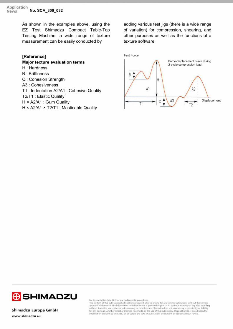
As shown in the examples above, using the EZ Test Shimadzu Compact Table-Top Testing Machine, a wide range of texture measurement can be easily conducted by
adding various test jigs (there is a wide range of variation) for compression, shearing, and other purposes as well as the functions of a texture software.
[Reference] Major texture evaluation terms H : Hardness B : Brittleness C : Cohesion Strength A3 : Cohesiveness T1 : Indentation A2/A1 : Cohesive Quality T2/T1 : Elastic Quality H × A2/A1 : Gum Quality H × A2/A1 × T2/T1 : Masticable Quality
Test Force
Displacement
Force-displacement curve during 2-cycle compression load
No. SCA_300_032

■ Introduction The Japanese Consumer Affairs Agency, Food Labeling Div. Notification No. 277 (Labeling requirements for special-application foods) specifies standards for labeling foods intended for people who have difficulties swallowing. The following describes a system able to easily measure the parameters to
determine conformance to the evaluation standards – hardness, adhesiveness, and cohesiveness. It was possible to determine which standard range was applicable by measuring food intended for nursing care applications and comparing characteristic values to the specified standards.
Jig for Evaluation Test of Foods for People with Difficulty Swallowing
Evaluation Test Results of Foods for People with Difficulties Swallowing
Material Testing System EZ-Test
Evaluation Test of Foods for People with Difficulties Swallowing No. SCA_300_042

• Test speed: 10 mm/sec
• Stroke Displacement: 10 mm
• Repetitions: 2
• Test Temperature: 20 °C℃
Sample Hardness (N/m2) Adhesiveness (J/m3) Cohesiveness Standard
(judgment)
Corn soup 0,805 X103 0,129 X103 0,78 III
Boiled meet and potato 1,04 X10⁴ 0,246 X103 0,21 III
Cream sauce 1,07 X10³ 0,206 X103 0,78 II
Table 1: Test Results
Test Method for Foods for People with Difficulty Swallowing (CAA, Food Labeling Div., Notification No. 277). Fill samples to a height of 15 mm in a container 20 mm tall and 40 mm in diameter (a 15 mm tall container is acceptable if there is no possibility of sample overflowing). Use an instrument capable of measuring compressive stress by means of a liner motion to measure compressive stress two times using a plastic plunger 8 mm tall and 20 mm in diameter to compress samples at a rate of 20 mm/sec, with a bottom clearance of 5 mm.
The measurement temperature ranges are within 10 °C ±2 °C and within 20 °C ±2 °C for foods served cooled or at room temperature, and within 20 °C ±2 °C and within 45 °C±2 °C for foods served heated.
Testing Jig
Standard Allowable Range I Allowable Range II Allowable Range III
Hardness[N/m2] (resistance to compression applied at constant speed)
2,5 X10³ - 1X10⁴ 1 X10³ - 1,5X10⁴ 3 X10² - 2X10⁴
Adhesiveness (J/m3) Max. 4 X10² Max. 1 X10³ Max. 1,5 X10³
Cohesiveness 0,2 – 0,6 0,2 – 0,9 -----
No. SCA_300_042

Today, Japanese people eat more pork than any other type of meat, 10 kg per person per year. Let's look at the history of eating pork in Japan. Generally, it is believed that Japanese people started to eat pork in the Meiji Era (1868-1912). In ancient times, they ate wild boar meat. It has been discovered that people kept wild boar during the Yayoi Era (1000 BC to 300 AD). It is imagined that people kept them free-range instead of penned in cages, fed them leftover food scraps, and ate them during festivals or special occasions. People nowadays like tender meat more than chewy meat.
Therefore, various measures are taken to make pork tender, for example by soaking it in water or in protein degrading enzyme solution to quickly achieve an adequate level of tenderness. Two cuts of store-bought Boston pork butt were soaked for 20 hours, one in water and the other in a protein degrading enzyme solution. A penetrating strength test was then performed on them and their textures were converted into numerical values for comparison. Fig. 1 is the penetrating test force- penetrating depth curve of store-bought Boston pork butt. Fig. 2 shows how the penetrating strength test was performed
Fig. 1 Penetrating Test Force- Penetrating Depth Curve on Store-Bought Boston Pork Butt
Fig. 2 Penetrating Strength Test being performed on Pork
Material Testing System EZ-Test
Measurement of Texture of Pork by a Penetrating Strength Test
No. SCA_300_046

The EZ Test Shimadzu Table-Top Universal Tester was used in the test. Fig. 3 is the penetrating test force-penetrating depth curve of pork soaked in
water for 20 hours. Fig. 4 shows the results of soaking meat in a protein degrading enzyme solution for 20 hours.
Fig. 3 Curve of Pork soaked in Water for 20 Hours In these tests, the strength was measured at the point where a 5 mm diameter penetration elasticity jig penetrated a 20 mm thick cut of Boston Pork Butt to a depth of 10 mm at a speed of 100 mm/min. When the results shown in Fig. 3 and Fig. 4 are compared, the jig went deeper into the pork soaked in enzyme solution for 20 hours as compared to the pork soaked in water for 20 hours when the same test force was used, indicating the former is more tender.
Fig. 4 Curve of Pork soaked in Enzyme Solution for 20 Hours When Fig. 1 and Fig. 3 are compared, approximately four times the strength is necessary to penetrate store-bought pork to the same depth as pork soaked in water for 20 hours, clearly indicating the difference in hardness. As shown in these figures, the texture of pork was converted into numerical values from the pork penetrating test strength- penetrating depth curve. Table 1 below shows the maximum penetrating test strength of these three tests.
Table 1
Sample Average Value of Maximum Test Force N
Store-Bought Boston Pork Butt 3.90
Boston Pork Butt Soaked in Water for 20 hours 0.98
Boston Pork Butt Soaked in Enzyme Solution for 20 hours 0.49
No. SCA_300_046

The EZ Test Shimadzu Table-Top Universal Tester can be used to convert texture-related properties such as crispness of croquettes, resilience of bread, and firmness of boiled
fish paste (kamoboko) as well as tenderness of pork reported in this document.
No. SCA_300_046

■ Introduction Plum is not only a food but also used as a medicinal foodstuff to recover from fatigue and treat food poisoning. There are many types of plums such as the well-known Gojiro, Shirakaga, Sugita, Akebono, and Nankoh varieties. Yellowish unripened plums are used to make pickled plums and plum wine. Texture and smell of four types of store-bought plums pickled in plum wines were converted into numerical values for comparison. The analysis and measurement items are listed below.
(1) Measurement of hardness and elastic quality which corresponds to chewiness using the EZ Test Shimadzu Compact Table-Top Testing Machine X-Ray Inspection System to see how pickled it is.
(2) Fluoroscopy of the inside of fruit flesh using the SMX-1000 Shimadzu Microfocus X-Ray Inspection System to see how pickled it is.
■ Measurement of Elastic Quality of Pickled Plums Fig. 1 is a photo of elasticity measurement where fruit flesh was penetrated to a depth of 6 mm twice by a 0.5R penetration elasticity test jig.
Fig. 1 Penetrating Test Performed on Pickled Plum
Figs. 2-1 to 2-4 show the force (penetrating resistance [N]-vertical axis)-displacement (penetrating depth [mm]-horizontal axis) curves obtained using TRAPEZIUMX Texture software. In the curves, the higher the highest peak is, the harder the plum. The deeper the lower peak of the curve below the horizontal
axis is, the higher the cohesiveness. And, the greater the height ratio between the height of the moderate curve slightly above the horizontal axis and the highest peak is, the higher the elasticity. In the test performed, the result was A≈B>D>C for all hardness, elastic quality, and cohesiveness.
Material Testing System EZ-Test
Multifaceted Measurement of Plums Pickled in Plum Wine No. SCA_300_048

Fig. 2-1 Pickled Plum A Fig. 2-2 Pickled Plum B
Fig. 2-3 Pickled Plum C Fig. 2-4 Pickled Plum D
■ Fluoroscopic Observation of the Inside of Pickled Plums Using the X-Ray Inspection System X-ray fluoroscopy was performed on pickled plums A through D at a certain fluoroscopic magnification and resolution (X-ray tube voltage 90 kV, X-ray tube current 110 μA, magnification 5×). The results are shown in Figs. 3-1 to 3-4. In general, areas with a higher density are displayed darker (blacker) and areas with a lower density are displayed lighter (whiter) in fluoroscopic images.
In Figs. 3-1 to 3-4, darkness of pickled plums A and B are similar, which indicates that the density of fruit flesh is relatively high. The entire fruit flesh of pickled plum C looks whitish, which indicates that liquid (distilled spirit in this case) has penetrated. In pickled plum D, a portion of fruit flesh close to the skin looks swollen because of liquid.
Fig. 3-1 Pickled Plum A
Fig. 3-2 Pickled Plum B
No. SCA_300_048

Fig. 3-3 Pickled Plum C
Fig. 3-4 Pickled Plum D
According to the above, the degree of penetration of distilled spirit (degree of swelling) was evaluated to be A≈B>C>D. The result was the same as how people felt (how pickled the plums were) when they put the plums in their mouth. However, the order of plums for hardness, elasticity, and cohesiveness was different from the data.
Fig. 4 SMX-1000 Shimadzu Microfocus X-Ray Inspection System
■ Summary In the test, pickled plums were evaluated by a mechanical test, image observation. Although the results were sufficiently convincing,
multifaceted analysis and measurement are believed to help convert the texture of food into numerical values.
No. SCA_300_048

■ Introduction The evaluation of the mechanical properties of foods, such as strength and hardness, is becoming widely used for the numerical comparison and control of food texture. This Application News introduces the tensile test and cutting test of Japanese soumen vermicelli to evaluate the texture. Soumen vermicelli is originated in Nara Prefecture in Japan. It was made by hand by kneading
wheat, salt and water; applying food oil and starch; and then stretching, drying, and maturing. Nowadays, it is generally machine-made. According to JAS (Japan Agricultural Standards) standards, noodles less than 1.3 mm diameter are "soumen"; those from 1.3 mm to 1.7 mm diameter are "hiyamugi"; and larger noodles are classified as "udon”.
■ Testing Equipment and Specimens Two types of commercially available soumen (Sample A, Sample B) were used as specimens for these tests. However, the diameters varied between 0.8 mm and 1.3 mm due to the degree of drying (the state in which it was sold). Therefore, the noodle diameters were measured with Vernier calipers to select specimens of approximately the same diameter. The specimens were added to boiling water and boiled for three minutes and then washed in cold water for ten seconds. Ten specimens each of Sample A and Sample B were tested within five minutes. Testing was performed using a Shimadzu EZTest tabletop tester (Fig. 1).
Fig. 1 EZTest Tabletop Tester
■ Tensile Test The specimens were grasped in grips (sponge was attached to the grip faces to prevent destruction of the specimens), and the grips were mounted in the tester through universal joints. Tensile test was performed under the following conditions:
1) Force measurement - Load cell (1 N) 2) Extension measurement - Internal
extensometer in tester 3) Test speed - 50 mm/min. Fig. 2 and Fig. 3 show an overview of the grips and a specimen mounted in the tester.
Material Testing System EZ-Test
Texture Analysis of “Soumen” Japanese Vermicelli No. SCA_300_051

Sample A
Displacement (mm)
Sample B
Displacement (mm)
Grip face with sponge
Specimen
Fig. 2 Grips for Tensile Test
Fig. 4 shows the tensile test results as force-displacement (extension) curves. (Curves are superimposed for all ten specimens). The results indicate a maximum force of 164 mN and break displacement of 56 mm for Sample A and 120 mN. maximum test force and break displacement of 37.8 mm for
Upper grip Specimen Lower grip
Fig. 3 Overview of Tensile Test
Sample B. Sample A exhibits greater extension and strength than Sample B. (All values are averages of ten samples.)
Fig. 4 Tensile Test Results
■ Cutting Test Cutting test can be performed as an evaluation method that approximates biting through foods. For cutting test, the specimen is placed on the compression plate and the cutting test jig (tooth-shape press: R 0.2 mm knife-edge tip) is pressed down on the sample from above. The test conditions are as follows: 1) Force measurement - Load cell (1 N). 2) Indentation measurement - Internal
extensometer in tester. 3) Test speed - 5 mm/minute.
Fig. 5 shows a specimen mounted in the tester.
Cutting test jigs (tooth shape) Specimen Compression plate
Fig. 5 Overview of Cutting Test
No. SCA_300_051

Fig. 6 shows the cutting test results as force-displacement (indentation) curves. (Curves are superimposed for all ten specimens.)
The results indicate a maximum force of
207 mN for Sample A and 129 mN maximum test force for Sample B. (All values are averages of ten samples.)
Fig. 6 Cutting Test Results
The tensile and cutting test results above provide a numerical evaluation that Sample A has a firmer texture than Sample B.
The results confirm that the materials tester is effective for quantification for functional testing.
Sample A Sample B
No. SCA_300_051

■ Introduction The numeric quantification of sensations has become increasingly important in recent years to provide the basic information for the accurate determination, improvement, and differentiation of the goods that surround us in our everyday lives. Sensations were conventionally evaluated mainly by the human five senses. However, numeric quantification of sensations is an effective method for the improvement and differentiation of goods. In the food industry, in particular, the quantitative evaluation of food texture is now commonly used for various purposes including the quality control and development of new food products. The Shimadzu EZTest texture analyzer offers dedicated texture-analysis software and a comprehensive range of specialized test jigs for the quantitative evaluation of food texture, including crunchiness, crispiness, and palatability. It is a general-purpose tester that can be used for the strength testing of packaging materials in addition to the development, improvement, and quality control of foods. This Application News introduces the use of EZTest for the texture analysis of salted salmon roe from different regions. ■ Testing Equipment and Test Conditions Two samples of salted salmon roe (Sample A, Sample B) produced in different areas were tested. Testing was performed using a Shimadzu EZTest texture analyzer (Fig. 1).
Fig. 1 Overview of EZTest Texture Analyzer
EZTest features a compact frame that is extremely easy to operate. In addition to texture analysis, it can be used for the strength testing of other small samples. Table 1 shows the configuration of the tester used, including the accessories.
Table 1 Tester Configuration Main unit EZTest EZ-S-5N
Load cell Capacity 5 N
Jig 15 mm dia. compression plate (upper)
Software TRAPEZIUM Rheometer texture analysis software
The texture was evaluated under compressive loads. Table 2 lists the test conditions and Fig. 2 shows an overview of the progress of a test.
Material Testing System EZ-Test
Texture Analysis of "Ikura" Salted Salmon Roe by EZTest No. SCA_300_052

Table 2 Test conditions
Test mode
Compression test (One egg from the salmon roe is placed on the compression plate and subjected to compressive oads.)
Test speed 10 mm/minute (constant speed)
Stroke 3 mm (Stroke to crush roe after compression.)
Ambient temperature 20 ˚C
Ambient humidity 60 %
Fig. 2 Overview of Texture Testing of Salted Salmon Roe
Table 3 Test Results Sample Name Hardness (N) Breaking Strength
A 0.54 0.02 B 1.38 0.08
* Hardness: Maximum test force under compression Breaking strength: Maximum stress calculated from maximum test force and size of the egg
Fig. 3 Test Force-Stroke Curves for Typical Samples
These curves indicate that Sample A achieves over twice the hardness and breaking strength values of Sample B. Differences in the failure process of roe are also apparent. These differences are sensed
as differences in texture, which can be difficult to express. Therefore, numeric quantification offers the advantage of providing an indicator for the quantitative comparison of food textures.
Sample A Sample B
Texture Analysis of "Ikura" Salted Salmon Roe 2
1.8
1.6
1.4
0 0 0.5 1 1.5 2 2.5 3 3.5 4 4.5 5
Stroke (mm)
Test
forc
e (N
)
No. SCA_300_052
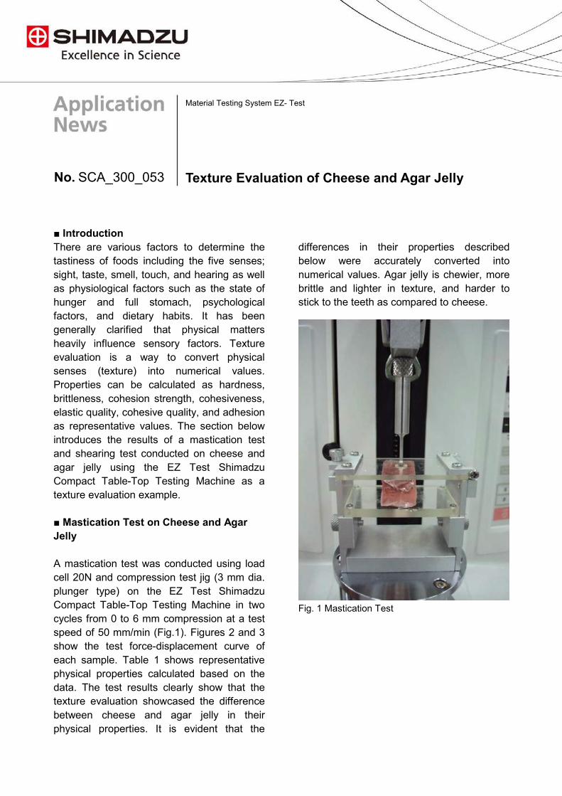
■ Introduction There are various factors to determine the tastiness of foods including the five senses; sight, taste, smell, touch, and hearing as well as physiological factors such as the state of hunger and full stomach, psychological factors, and dietary habits. It has been generally clarified that physical matters heavily influence sensory factors. Texture evaluation is a way to convert physical senses (texture) into numerical values. Properties can be calculated as hardness, brittleness, cohesion strength, cohesiveness, elastic quality, cohesive quality, and adhesion as representative values. The section below introduces the results of a mastication test and shearing test conducted on cheese and agar jelly using the EZ Test Shimadzu Compact Table-Top Testing Machine as a texture evaluation example. ■ Mastication Test on Cheese and Agar Jelly A mastication test was conducted using load cell 20N and compression test jig (3 mm dia. plunger type) on the EZ Test Shimadzu Compact Table-Top Testing Machine in two cycles from 0 to 6 mm compression at a test speed of 50 mm/min (Fig.1). Figures 2 and 3 show the test force-displacement curve of each sample. Table 1 shows representative physical properties calculated based on the data. The test results clearly show that the texture evaluation showcased the difference between cheese and agar jelly in their physical properties. It is evident that the
differences in their properties described below were accurately converted into numerical values. Agar jelly is chewier, more brittle and lighter in texture, and harder to stick to the teeth as compared to cheese.
Fig. 1 Mastication Test
Material Testing System EZ- Test
Texture Evaluation of Cheese and Agar Jelly No. SCA_300_053

Fig. 2 Force-Displacement Curve for Cheese
Fig. 3 Test Force-Displacement Curve for Agar Jelly
Parameter Hardness Cohesion Strength Cohesiveness Indentation Cohesive
Quality Elastic Quality
Gum Quality
Masticable Quality
Unit N N J mm
Agar Jelly 4.48 -0.04 -0.0001 5.58 203.358 1.08529 916.504 988.558
Cheese 0.77 -0.25 -0.00095 2.84 132.789 2.14723 102.315 220.447 Table 1 Texture Evaluation Values of Cheese and Agar Jelly (Mastication Test)
■ Shearing Test on Cheese and Agar Jelly A shearing test was conducted using a shearing jig to evaluate hardness and chewiness as evaluation examples just like the mastication test described above. (Fig.4) Figs.5 and 6 show the force-displacement curve of each sample as the test results. The data also clearly indicate the difference between the properties of cheese and agar jelly.
Fig. 4 Shearing Test
Fig. 5 Force-Displacement Curve for Cheese
Fig. 6 Test Force-Displacement Curve for Agar Jelly
No. SCA_300_053

As shown in the examples above, using the EZ Test Shimadzu Compact Table-Top Testing Machine, a wide range of texture measurement can be easily conducted by adding various test jigs (there is a wide range of variation) for compression, shearing, and other purposes as well as the functions of a texture software.
[ Reference] Major texture evaluation terms
H : Hardness B : Brittleness C : Cohesion Strength A3 : Cohesiveness T1 : Indentation
A2/A1 : Cohesive Quality T2/T1 : Elastic Quality H × A2/A1 : Gum Quality H × A2/A1 × T2/T1 : Masticable Quality
Test Force
Displacement
Force-displacement curve during 2- cycle compression load
No. SCA_300_053

6. Metal Industry

6. Metal Industry
DESTRUCTIVE AND NON-DESTRUCTIVE TESTING
The metal industries cover non-ferrous metals (e.g. aluminium, copper and zinc) and ferrous materials such as iron and steel. From an economic perspective, iron is the most important metal and is used in steel, cast iron and many alloys.
In ancient times, metals have been drivers of human culture and civilization. Today, they are the backbone of many indus-tries and are used in uncountable products and applications. Main buyers are the automotive, construction and manufac-turing, and mechanical engineering industries. Although processing of iron is an approx. 3000 years old technology, the steel industry is innovative, and many steel qualities have been developed in recent years.
Metals are tested mostly with two methods: non-destructive testing (NDT) and destructive testing (Destructive Physical Analysis DPA). Non-destructive testing evaluates properties of materials and components without damaging them. Using different methods, destructive testing examines specimens in order to understand their performance, failure and material behavior.
Stress, crash and hardness tests are typical destructive testing methods. They are easier to carry out than non-destructive testing, and deliver more information which is easier to inter-pret. Where significant hazard or economic loss can occur, non-destructive testing is the method of choice for prevention of component failure.

6. Metal Industry
C225-E032 Ultrasonic fatigue testing system with an average stress loading mechanism
No_i244 Tensile test for metallic materials using strain rate control and stress rate control
No.14 Tensile testing metallic materials stress rate contro lKM
No.15 Tensile testing metallic materials strain rate contro lKM
SCA_300_023 Measurement of carburized case depth of steel with Shimadzu micro hardness tester model HMV i45
SCA_300_024 Measurement of hardness of the machining deterioration layer of stainless steel with Shimadzu dynamic ultra micro hardness tester DUH
SCA_300_034 A hardness measurement of steel surface treatment layer with Shimadzu dynamic ultra micro hardness tester, model DUH
SCA_300_035 A hardness measurement of surface treat- ment layer on a steel sample using Shimadzu dynamic ultra micro hardness tester, model DUH
SCA_300_036 A thickness measurement of a Ni-plating layer on a stainless-steel sample with Shimadzu dynamic ultra micro hardness tester, mode DUH
SCA_300_045 Jigs for measuring Bauschinger effect
SCA_300_047 Measurement of the surface treatment depth of steel with Shimadzu micro hardness tester model HMV
SCA_300_050 Strength evaluation on metallic fine particles with Shimadzu micro compression testing machine model MCT
SCA_300_061 Compressive strength of metallic micro- spheres and dependence on heat treatment temperature MCT
eV021 Observation of bending fatigue testing of metal plate at ultrasonic frequency

C225-E032
Ultrasonic Fatigue Testing System Effective for Gigacycle Fatigue Tests
With fatigue tests of high-strength steels, it is evident that internal fracture (fish-eye fracture), which is caused by inclusions and other micro defects, occurs at 107 cycles or more, a value considered the conventional fatigue limit.An ultrasonic fatigue testing system is extremely effective when performing this sort of gigacycle fatigue test. (With a 100 Hz fatigue testing system, this would take 3 years, but if a 20 kHz ultrasonic fatigue testing system is used, testing can be completed in one week.)
Actual components are rarely used under conditions in which the average stress is zero. Despite this, the USF-2000A, a standard ultrasonic fatigue testing system, can only perform testing under zero average stress conditions.Using an ultrasonic fatigue testing system equipped with an average stress loading mechanism, gigacycle fatigue tests can be performed with average tensile stress loaded.
Ultrasonic Fatigue Testing System with an Average Stress Loading Mechanism
Stressdistribution
AG-X5kNAverage stress loading
High-rigidity booster
Horns
High-rigidity booster
5 kN load cellAverage stress measurement
Converter(Piezo actuator)
Strain GaugeSamples
DisplacementStress
System Appearance
For Gigacycle Fatigue Tests with Average Stress Loaded

© Shimadzu Corporation, 2016First Edition: August 2016
For Research Use Only. Not for use in diagnostic procedure. This publication may contain references to products that are not available in your country. Please contact us to check the availability of these products in your country.Company names, product/service names and logos used in this publication are trademarks and trade names of Shimadzu Corporation or its affiliates, whether or not they are used with trademark symbol “TM” or “®”. Third-party trademarks and trade names may be used in this publication to refer to either the entities or their products/services. Shimadzu disclaims any proprietary interest in trademarks and trade names other than its own.
The contents of this publication are provided to you “as is” without warranty of any kind, and are subject to change without notice. Shimadzu does not assume any responsibility or liability for any damage, whether direct or indirect, relating to the use of this publication.www.shimadzu.com/an/
Ultrasonic resonance systemPower supply, converter, booster (1 pair), horn (1 pair)
Personal computer(OS Windows 7) ADA/PIO interface board
SoftwareUltrasonic test control measurement software
Cooling systemAir dryer, air piping• A separate 140 L/min air source is required.
5 Strain meter unit (option)
6 AG-X plus Autograph 5 kN + 250 extension
7 Average stress loading mechanism
1
2
3
4
Main Speci�cations
1) Test Frequency: 20 kHz ± 500 Hz
• The recommended test range is 20 kHz ± 30 Hz.• The test frequency is determined by the resonance frequency of the sample.
2) Horn End Face Amplitude
Min. approx. ±10 μmMax. approx. ±50 μm
• The minimum and maximum amplitudes are the end face amplitude values at amplitude outputs of 20 % and 100 % respectively. Accordingly, the minimum and maximum amplitude values will change somewhat depending on the shape of the sample.
4) Average Stress
Max. 1.5 kN (tensile only)
3) Test Stress
Standard circular tapered sampleStress Min. 237 MPa Max. 1186 MPa• The test stress range can be changed by changing the sample shape.• The minimum and maximum values are calculated with the end face amplitude values of 10 μm and 50 μm respectively.• These are the values when the stress is within the elasticity range.
Standard Circular Tapered Sample
Surface of the Fatigued Fracture Originating from the Inclusion
Center hole can remain
Center holecan remain
Components

ApplicationNews
No.
LAAN-A-AG-E009
Material Testing System
Tensile Test for Metallic Materials Using Strain Rate Control and Stress Rate Control
i244International standards for tensile testing of metallic materials have been revised as specified in ISO 6892 and JIS Z2241, such that strain rate control, where strain is measured with an extensometer, has recently been added as a test item to the current stress rate control method, in which a load is applied to a material until its yield point is reached. As a result, it can be assumed that there will be situations where both stress rate control and strain rate control tensile testing of
metallic materials will be required.Here, we introduce examples of strain rate control and stress rate control tensile testing of metallic samples, including cold-rolled steel, austenitic stainless steel, aluminium alloy and brass, according to ISO 6892, using the Shimadzu Autograph AG-50kNX Precision Universal Tester, and the SSG50-10H strain gauge type one-touch extensometer (Fig. 1, Fig. 2).
Table 1 Test Specimens
Information on the sample specimens are shown in Table 1, and the test conditions are shown in Table 2.
n Introduction
n Specimens and Test Conditions
Fig. 1 Overview of Universal Testing System Fig. 2 Specimen and Jigs for Tensile Testing
Sample Name A B C D
Material Cold-rolled steel Stainless steel (austenitic) Aluminium alloy Brass
Sample size
Width 25 mm, thickness 1 mm, gauge length 50 mm, parallel length 60 mm(JIS Z 2241 No. 5 test specimen)
Gauge length
50 mm
Parallel length60 mm
Width 25 mm

Table 2 Test Conditions
1) Load cell capacity 50 kN
2) Jig 50 kN Non-shift wedge type grips (file teeth for flat specimen)
3) Test speed See Table 3
4) Test temperature Ambient temperature
5) Software TRAPEZIUMX (single)
Fig. 3 shows an image diagram of the test speed, and Table 3 and Table 4 show the applicable test speeds for the strain control and stress control tests, respectively.
Table 3 Test Strain Rate (based on strain rate control)
V1: Strain rate 0.00025/s (1.5 %/min)
V2: Strain rate 0.00025/s (1.5 %/min)
V3: Predicted strain rate 0.0067/s (40 %/min)
Table 4 Test Stress Rate (based on stress rate control)
V1: Stress rate 10 MPa/s
V2: Strain rate 0.00083/s (5 %/min)
V3: Predicted strain rate 0.0067/s (40 %/min)
Table 5 Test results (Average n = 3)
Sample NameElastic
Modulus (GPa)
0.2 % Proof Strength
(MPa)
Tensile Strength
(MPa)
Elongation at Break
(%)
A (cold-rolled steel) 194 185.5 341.5 43.3
B (stainless steel) 200 278.5 660.8 55.0
C (aluminum) 71 170.1 236.3 13.0
D (brass) 109 193.1 398.1 49.1
(A): Upper yield point (or its corresponding point)(B): Upper limit of strain measurement (point after proof strength point)
Note 1) Strain rate refers to the amount of increase in strain, obtained using an extensometer to measure the gauge length of a test specimen, per unit time.
Note 2) Predicted strain rate was obtained using the displacement of the testing machine crosshead at each point in time and the test specimen's parallel length. Thus, it is defined as the increase in strain of the specimen's parallel length per unit time.
Fig. 3 Image of Test Strain Rate
Strain (%)(A) (B)
Stre
ss (M
Pa)
V2
V1
V3
F ig. 4 shows a d iagram of the st ress – s t roke displacement for each sample using strain-rate control, and Table 5 shows their characteristic values. In Fig. 4, the point at which the stress becomes discontinuous, as indicated by the jump in the stress-stroke displacement curve, corresponds to the point at which the strain rate is switched.
n Test Results
Fig. 4 Test Results for Each Metallic Material (stress-stroke curve based on strain rate control)
Stroke Displacement (mm)
Stre
ss (M
Pa)
800
700
600
500
400
300
200
100
00 20 40 60 80
ABCD
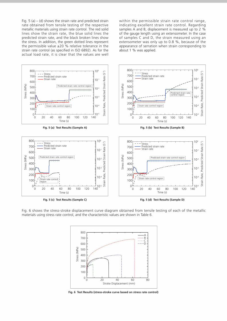
Fig. 6 Test Results (stress-stroke curve based on stress rate control)
Fig. 5 (a) – (d) shows the strain rate and predicted strain rate obtained from tensile testing of the respective metallic materials using strain rate control. The red solid lines show the strain rate, the blue solid lines the predicted strain rate, and the black broken lines show the stress. In addition, the green dotted lines represent the permissible value ±20 % relative tolerance in the strain rate control (as specified in ISO 6892). As for the actual load rate, it is clear that the values are well
within the permissible strain rate control range, indicating excellent strain rate control. Regarding samples A and B, displacement is measured up to 2 % of the gauge length using an extensometer. In the case of samples C and D, the strain measured using an extensometer was only up to 0.8 %, because of the appearance of serration when strain corresponding to about 1 % was applied.
Fig. 6 shows the stress-stroke displacement curve diagram obtained from tensile testing of each of the metallic materials using stress rate control, and the characteristic values are shown in Table 6.
Fig. 5 (a) Test Results (Sample A)
0 20 40 60 80 100 120 1400
100
200
300
400
500
600
700
800Stress
10-5
10-4
10-3
10-2
10-1
100
Strain rate control region
Predicted strain rateStrain rate
Predicted strain rate control region
Stre
ss (M
Pa)
Stra
in R
ate,
Pre
dict
ed S
trai
n Ra
te (S
-1)
Time (s)
Fig. 5 (b) Test Results (Sample B)
0 20 40 60 80 100 120 140
Strain rate control region
StressPredicted strain rateStrain rate
0
100
200
300
400
500
600
700
800
10-5
10-4
10-3
10-2
10-1
100
Predicted strain rate control region
Stre
ss (M
Pa)
Stra
in R
ate,
Pre
dict
ed S
trai
n Ra
te (S
-1)
Time (s)
Fig. 5 (c) Test Results (Sample C)
0 20 40 60 80 100 120 140
Strain rate control region
StressPredicted strain rateStrain rate
0
100
200
300
400
500
600
700
800
10-5
10-4
10-3
10-2
10-1
100
Predicted strain rate control region
Stre
ss (M
Pa)
Stra
in R
ate,
Pre
dict
ed S
trai
n Ra
te (S
-1)
Time (s)
Fig. 5 (d) Test Results (Sample D)
0 20 40 60 80 100 120 140
Strain rate control region
StressPredicted strain rateStrain rate
0
100
200
300
400
500
600
700
800
10-5
10-4
10-3
10-2
10-1
100
Predicted strain rate control region
Stre
ss (M
Pa)
Stra
in R
ate,
Pre
dict
ed S
trai
n Ra
te (S
-1)
Time (s)
Stroke Displacement (mm)
Stre
ss (M
Pa)
800
700
600
500
400
300
200
100
00 20 40 60 80
ABCD

For Research Use Only. Not for use in diagnostic procedures.The contents of this publication are provided to you “as is” without warranty of any kind, and are subject to change without notice. Shimadzu does not assume any responsibility or liability for any damage, whether direct or indirect, relating to the use of this publication.
First Edition: January, 2012
www.shimadzu.com/an/ © Shimadzu Corporation, 2012
Fig. 7 (a) – (d) shows the strain rate and predicted strain rate obtained from tensile testing of the respective metallic materials using stress rate control. The pink
solid lines show the stress rate, the blue solid lines the predicted strain rate, and the black broken lines show the stress.
It is clear that at the set rates, suitably stable data could be acquired for both stress rate and predicted strain rate.The above results demonstrate that in the tensile testing of the various types of metallic materials using the Shimadzu Autograph AG-50kNX Precision Universal Tester, the strain rate control values were well within the range of the permissible values (± 20 %) specified in ISO 6892. Similarly, stable testing using stress rate control was also achieved. When using typical universal
testing machines, testing control methods other than the crosshead rate control, e.g. strain rate control and stress rate control, normally require burdensome adjustment of the control gain depending on the material being tested. However, with this instrument, strain rate control and stress rate control in tensile testing of any metallic material are easily conducted because the gain is adjusted automatically (auto-tuning feature).
Fig. 7 (a) Test Results (Sample A)
0
10
20
30
40
50
60
70Stress × 0.1Stress rate
10-5
10-4
10-3
10-2
10-1
100
Predicted strain rate
0 20 40 60 80 100 120 140
Stre
ss R
ate
(MPa
/s),
Stre
ss (M
Pa)
Pred
icte
d St
rain
Rat
e (S
-1)
Time (s)
Fig. 7 (b) Test Results (Sample B)
Stress × 0.1Stress rate
Predicted strain rate
0
10
20
30
40
50
60
70
10-5
10-4
10-3
10-2
10-1
100
0 20 40 60 80 100 120 140
Stre
ss R
ate
(MPa
/s),
Stre
ss (M
Pa)
Pred
icte
d St
rain
Rat
e (S
-1)
Time (s)
Fig. 7 (c) Test Results (Sample C)
Stress × 0.1Stress rate
Predicted strain rate
0
10
20
30
40
50
60
70
10-5
10-4
10-3
10-2
10-1
100
0 20 40 60 80 100 120 140
Stre
ss R
ate
(MPa
/s),
Stre
ss (M
Pa)
Pred
icte
d St
rain
Rat
e (S
-1)
Time (s)
Fig. 7 (d) Test Results (Sample D)
Stress × 0.1Stress rate
Predicted strain rate
0
10
20
30
40
50
60
70
10-5
10-4
10-3
10-2
10-1
100
0 20 40 60 80 100 120 140
Stre
ss R
ate
(MPa
/s),
Stre
ss (M
Pa)
Pred
icte
d St
rain
Rat
e (S
-1)
Time (s)
Table 6 Test Results (Average n = 3)
Sample NameElastic Modulus
(GPa)0.2 % Proof Strength
(MPa)Tensile Strength
(MPa)Elongation at Break
(%)
A (cold-rolled steel) 194 193.3 349.3 42.0
B (stainless steel) 205 290.7 687.0 54.8
C (aluminum) 69 177.0 233.5 12.6
D (brass) 112 196.7 405.5 48.8

14
LAAN-J-AG0014
Material Testing & Inspection
Standard No. ISO6892:2009 (JIS Z 2241: 2011)
Autograph Precision Universal Tester
Introduction
Metallic materials have excellent extensibility and ductility and are comparatively easy to mechanically process. Consequently, they are widely used in industrial components, building materials, and everyday goods. Tensile tests using stress rate control have long been used for quality control and new material development as a means of evaluating the mechanical properties of metallic materials. This Application Data Sheet introduces examples of static tensile testing using stress rate control performed on dumbbell-shaped test specimens of 4 types of metallic materials (cold-rolled steel, austenitic stainless steel, aluminium alloy, brass), in which basic mechanical properties such as tensile strength and elongation are evaluated. T. Murakami
Most metallic materials have tensile strengths higher than those of resin and rubber materials, so it is necessary to select grips that are capable of reliably and stably holding the material during testing up to fracture. For tensile testing of metallic materials, non-shift wedge-type or hydraulic grips are used for samples with a large test force. For samples with a small maximum test force, pneumatic flat and screw-type flat grips are also used.
Measurement and Jigs
Measurement Results
V1: Rate of increase of stress: 10 MPa/sV2: Estimated strain rate: 0.00084/s (5 %/min)V3: Estimated strain rate: 0.0067/s (40 %/min)Point of switching rate from V1 to V2: Point at which V1 exceeds V2 valuePoint of switching rate from V2 to V3: Point at which measurement of displacement by extensometer is terminated
Note: The estimated strain rate is obtained based on the displacement per unit time of the crosshead of the testing machine and the parallel length of the test specimen. It is the increment of strain in the parallel length of the test specimen per unit time.
Fig. 1: Image of Controlling Rates
Stre
ss (M
Pa)
Strain (%)
Width: 25 mm, thickness: 1 mm, gauge length: 50 mm, parallel length: 60 mm
Fig. 2: Sample Shape
Gauge length
Width 25 mm
Parallel length
Tensile Testing of Metallic Materials with Stress Rate Control
Table 1: Sample Information
Sample A B C DMaterial Cold-rolled steel Stainless steel Aluminum alloy Brass
Table 2: Test Results
Elastic modulus(GPa)
Proof strength (offset method)
(MPa)
Tensile strength(MPa)
Percentage elongationafter fracture
(%) A (Cold-rolled steel) 194 193.3 349.3 42.0B (Stainless steel) 205 290.7 687.0 54.8C (Aluminum alloy) 69 177.0 233.5 12.6D (Brass) 112 196.7 405.5 48.8
Sample

14
First Edition: February 2013
© Shimadzu Corporation, 2013www.shimadzu.com/an/
Shimadzu Corporation
Fig. 4 shows the stress rate and the estimated strain rate obtained from tensile testing the cold-rolled steel plate using stress rate control. It can be seen that stable data has been acquired in accordance with the set speed, for both the stress rate and estimated strain rate.
Features
A high-precision load cell is adopted. (The high-precision type is class 0.5; the standard-precision type is class 1.)Accuracy is guaranteed over a wide range, from 1/1000 to 1/1 of the load cell capacity. This supports highly reliable test evaluations.
Crosshead speed rangeTests can be performed over a wide range from 0.0005 mm/min to 1,000 mm/min.
High-speed samplingUltrafast sampling, as fast as 0.2 msec, allows assessment of sudden changes in test force, such as when brittle materials fracture.
TRAPEZIUMX X operational softwareDesigned for intuitive operation, it offers a variety of convenient and user-friendly features.
Smart controllerReal-time test force and position data are readily confirmed, and the manual dial enables fine adjustments to jig positioning.
Optional Test DevicesA variety of tests can be performed by switching between an abundance of jigs in the lineup.
Metal Stress Rate Control Tensile Testing System
AG-Xplus Floor-Type Precision Universal Tester
Tester: AG-XplusLoad Cell: 50 kN Test Jig: 50 kN non-shift wedge type gripsExtensometer: Strain gauge type one-touch extensometer: SSG50-10HSoftware: TRAPEZIUM X (Single)
0 20 40 60 800
100
200
300
400
500
600
700
800
応
力(M
Pa)
ストローク変位 (mm)
A B C D
Fig. 3:Stress–Stroke Displacement Curves for Each Metal Material
Stre
ss (M
Pa)
Stroke displacement (mm) 0 20 40 60 80 100 120 140
0
10
20
30
40
50
60
70 応力×0.1 応力速度
応力
速度
(M
Pa/
s)、
応力
(MP
a)
時間 (s)
10-5
10-4
10-3
10-2
10-1
100
推定ひずみ速度
推定
ひず
み速
度 (
s-1 )
Fig.4 速度結果例(試料A:冷間圧延鋼板)Time (s)
Estimated strain rateStress 0.1Stress rate
Stre
ss ra
te (M
Pa/
s), s
tress
(MP
a)
Est
imat
ed S
train
rate
(S-1
)
Fig. 4:Example of Stress Rate Results (Sample A: Cold-rolled steel plate)

15
LAAN-J-AG0015
Material Testing & Inspection
Standard No. ISO6892:2009 (JIS Z 2241: 2011)
Autograph Precision Universal Tester
Measurement Results
Fig. 1: Image of Controlling Rates
Stre
ss (M
Pa)
Strain (%)
Width: 25 mm, thickness: 1 mm, gauge length: 50 mm, parallel length: 60 mmFig. 2: Sample Shape
Gauge length
Width 25 mm
Parallel length
Introduction
The international standard for tensile testing of metallic materials, ISO 6892, includes a strain rate control test method (strain measurement with an extensometer). This is in addition to the conventional stress rate control method as the loading method up to the yield point of the material. It is expected that tensile testing of metallic materials using both stress rate control and strain rate control will increase in the future. As a result, many existing testing machine users are interested in whether or not it is possible to obtain stable data from both test methods using existing and/or new testing machines. This Application Data Sheet introduces examples of static tensile tests using strain rate control carried out on dumbbell-shaped test specimens of 4 types of metallic material (cold-rolled steel, austenitic stainless steel, aluminium alloy, brass), in which basic mechanical properties such as tensile strength and elongation are evaluated. T. Murakami
Table 1: Sample Information
Sample A B C DMaterial Cold-rolled steel Stainless steel Aluminum alloy Brass
Table 2: Test Results
Elastic modulus(GPa)
Proof strength (offset method)
(MPa)
Tensile strength(MPa)
Percentage elongationafter fracture
(%) A (Cold-rolled steel) 194 185.5 341.5 43.3B (Stainless steel) 200 278.5 660.8 55.0C (Aluminum alloy) 71 170.1 236.3 13.0D (Brass) 109 193.1 398.1 49.1
Sample
Tensile Testing of Metallic Materials with Strain Rate Control
V1, V2: Strain rate: 0.00025/s 20 % (feedback of strain from extensometer to testing machine)V3: Estimated strain rate: 0.0067/s (40 %/min) 20 %Point of switching rate from V2 to V3: Point at which measurement of displacement by extensometer is terminated(For samples A and B, displacement was measured using an extensometer up to 2 % of the gauge length. For samples C and D, serrations occurred when a strain equivalent to 1 % was applied, so measurement with the extensometer was used up to 0.8 %.)
Note: The estimated strain rate is obtained based on the displacement per unit time of the crosshead of the testing machine and the parallel length of the test specimen. It is the increment of strain in the parallel length of the test specimen per unit time.
Measurement and Jigs
Most metallic materials have tensile strengths higher than those of resin and rubber materials, so it is necessary to select grips that are capable of reliably and stably holding the material during testing up to fracture. For tensile tests of metallic materials, non-shift wedge-type or hydraulic grips are used for samples with a large test force. For samples with a small maximum test force, pneumatic flat and screw-type flat grips are also used.

15
First Edition: February 2013
© Shimadzu Corporation, 2013www.shimadzu.com/an/
Shimadzu Corporation
Features
A high-precision load cell is adopted. (The high-precision type is class 0.5; the standard-precision type is class 1.)Accuracy is guaranteed over a wide range, from 1/1000 to 1/1 of the load cell capacity. This supports highly reliable test evaluations.
Crosshead speed rangeTest can be performed over a wide range from 0.0005 mm/min to 1,000 mm/min.
High-speed samplingUltrafast sampling, as fast as 0.2 msec, allows the assessment of sudden changes in test force, such as when brittle materials fracture.
TRAPEZIUMX X operational softwareDesigned for intuitive operation, it offers a variety of convenient and user-friendly features.
Smart controllerReal-time test force and position data are readily confirmed, and the manual dial enables fine adjustments to jig positioning.
Optional Test DevicesA variety of tests can be performed by switching between an abundance of jigs in the lineup.
Metal Strain Rate Control Tensile Testing System
AG-Xplus Floor-Type Precision Universal Tester
Tester: AG-XplusLoad Cell: 50 kN Test Jig: 50 kN non-shift wedge type gripsExtensometer: Strain gauge type one-touch extensometer SSG50-10HSoftware: TRAPEZIUM X (Single)
0 20 40 60 800
100
200
300
400
500
600
700
800
応力
(MP
a)
ストローク変位(mm)
A B C D
Fig. 3: Stress-Stroke Curves
Fig. 3 shows an example of the strain rate and estimated strain rate obtained from tensile testing the cold-rolled steel plate using strain rate control. The red solid line indicates strain rate, the pink double dotted broken line indicates the estimated strain rate, and the blue broken line indicates the stress. The green dotted line indicates the tolerance of the strain increase rate (20 % specified by ISO 6892). The actual load rate is sufficiently within the tolerance of the strain rate control range, which indicates that good strain rate control has been performed.
Stre
ss (M
Pa)
Stroke displacement (mm) 0 20 40 60 80 100 120 140
0
100
200
300
400
500
600
700
800 応力
応力
(M
Pa)
時間 (s)
10-5
10-4
10-3
10-2
10-1
100
推定ひずみ速度制御部
ひずみ速度制御部
推定ひずみ速度 ひずみ速度
ひず
み速
度, 推
定ひ
ずみ
速度
(1/s)
Fig. 4:Example of Strain Rate Results (Sample A: Cold-rolled steel plate)
StressEstimated strain rateStrain rate
Estimated strain rate control section
Strain rate control section
Stre
ss (M
Pa)
Stra
in ra
te (1
/s),
Est
imat
ed s
train
rate
(1/S
)
Time (s)

■ Introduction Micro hardness testers are indispensable instruments for hardness evaluation, including surface composition, surface quenching layers, and machining transformation layers in research and development as well as quality control of parts of precision instruments, wires, metal foils, and electronic elements. The method for measuring the depth of layers hardened by carburizing or carburizing and quenching is specified in JIS-G-0557 "Method of measuring case depth hardened by carburizing treatment for steel." According to it, the effective depth or whole depth of hardened layer should be determined from the hardness distribution curve obtained on the cross section perpendicular to the hardened layer by use of a micro hardness tester. The Shimadzu Micro Hardness Tester, which features very high reliability and excellent operability due to its built-in data processing functions, is best suitable for efficient measurement of the depth of carburized layers. The following is an example of such a measurement.
■ Measurement of hardness distribution in a carburized layer of Ni-Cr-Mo steel A specimen was prepared by molding a cross section of steel into resin and finished by buffing. Hardness was measured at every 0.1mm on the test surface. The printer output is shown in Fig.1. The hardness distribution plotted from the measured data is shown in Fig.2 JIS-G-0557 defines the effective depth of hardened layer as the distance between the surface and the point at which Vickers hardness matches 550. In this test, the effective depth is 0.6 mm. Shimadzu Micro Hardness Tester, featuring completely automatic load change, loading, and unloading, is used for quality control of low to high hardness’s of small parts such as the gears and cams of watches, sewing machines, cameras and optical devices, and electronic elements like ICs and LSIs.
Material Testing System HMV-G
Measurement of Carburized Case Depth of Steel with Shimadzu Micro Hardness Tester Model HMV
No. SCA_300_023

Date of test Date 1987 2 14
Testing parameter file No File No. Specimen Number Sample No. Number of tests Test 13
Number of lots Lot 1
Testing mode Vickers
Type of specimen surface Flat Repetitive number to read data Read 2
Testing load Load 200 GF
Load duration time Loading Time 15 Sec
Correction coefficient Correct 0,1273 µm
Number of lots and number of tests for a specimen
Lot = 1, Test = 1
Diagonal length of the indentation D1 = 22,8
D2 = 22,6
Vickers hardness HV = 718
Lot = 1, Test = 2
D1 = 22,2
D2 = 22,6
HV = 735
Lot = 1, Test = 3
D1 = 22,3
D2 = 22,6
HV = 734
Lot = 1, Test = 4
D1 = 30,9
D2 = 31,5
HV = 380
Result of statistical calculation --Statistics--
Measuring mode HV
Number of lots Lot = 1
Mean hardness X = 572
Standard deviation S = 143,7
Coefficient of variation CV = 25,08 %
Minimum value in the lot Min. = 380
Maximum value in the lot Max. = 739
Fig. 1 Printer output of measured values
Fig. 2 Hardness Distribution in Carburized layer
* Please be advised that data obtained before the implementation of the current Weights and Measures Law may be presented in terms of gravimetric unit.
No. SCA_300_023

■ Introduction When a metallic material is processed with lathes, milling machines, or grinders, the upper portion of the material*s surface is transformed into a so-called machining deterioration layer. This layer, which results from plastic transformation and increased temperature during the machining process, comprises an amorphous layer, a plastic deterioration layer, a fine particle layer, and micro structure deterioration layers. These have greater displacement than the inner part of the material, producing residual stress. The following presents the results of dynamic indentation hardness testing on a thin surface layer (1-3 μm) of machine processed stainless steel (SUS304) performed with the Shimadzu Dynamic Ultra Micro Hardness Tester Model DUH. This machine is widely applicable to a range of hard to soft materials as it measures hardness of thin films and thin layers in terms of the indentation depth of an indenter (dynamic indentation hardness) or the diagonal length of indentation (Vickers hardness).
■ Test conditions 1) Specimen : Stainless steel SUS304 Processing:
A) Solution heat treatment only B) Polishing finish after solution heat
treatment C) Turning and polishing by polishing
paper after solution heat ■ Testing procedure Dynamic indentation hardness (hereafter called hardness) was calculated from the relation of load versus depth at 0.2 μm intervals from the surface with load being applied via indenter to each of three specimens finished in different ways. Load was continuously applied up to 100 gf. ■ Test results Table 1 displays the values measured under the processing condition A (others under processing conditions B and C are omitted), Table 2 the variation of hardness (averaged) along the depth direction for each of the processing conditions, and Fig.1 the depth versus hardness curves. The tendency of curve B to approach A at a depth of around 2 μm and to overlap A thereafter suggests that the machining deterioration layer remains influential until an indentation depth of around 2 μm, but the hardness of the matrix material is predominant thereafter. Curve C suggests that the respective machining deterioration layer keeps its influence down to a significantly greater depth than curve B, as sample C has undergone a turning process just prior to the polishing paper finish.
Material Testing System DUH
Measurement of Hardness of the Machining Deterioration Layer of Stainless Steel with Shimadzu Dynamic Ultra Micro Hardness Tester DUH No. SCA_300_024

No. SCA_300_024
No. Load (gf) Depth
Hardness 1 0.640 0.20 603.41 2 1.300 0.40 170.66 3 2.720 0.60 170.46 4 4.260 0.80 162.71 5 6.260 1.00 181.49 6 8.480 1.20 159.05 7 10.960 1.40 150.25 8 13.680 1.60 142.45 9 16.720 1.80 144.15 10 20.100 2.00 147.06 11 23.720 2.20 132.13 12 27.300 2.40 132.12 13 31.680 2.60 131.67 14 36.100 2.80 125.24 15 40.720 3.00 131.53 16 45.440 3.20 122.39 17 50.500 3.40 126.31 18 55.900 3.60 129.71 19 61.600 3.80 130.86 20 67.200 4.00 115.21 21 73.220 4.20 122.12 22 79.520 4.40 122.96 23 85.840 4.60 144.29 24 92.360 4.80 112.87 25 99.020 5.00 109.63
No. Load (gf) Depth
Hardness 1 0.700 0.20 662.16 2 1.620 0.40 179.93 3 2.940 0.60 184.68 4 4.600 0.80 175.00 5 6.460 1.00 149.01 6 8.760 1.20 165.34 7 11.220 1.40 143.00 8 14.020 1.60 147.37 9 17.040 1.80 139.21 10 20.440 2.00 146.18 11 23.900 2.40 127.990 12 27.640 2.40 128.53 13 31.500 2.60 124.12 14 35.880 2.80 129.77 15 48.580 3.00 136.78 16 45.360 3.20 123.04 17 50.420 3.40 126.32 18 55.340 3.60 108.31 19 61.00 3.80 130.32 20 66.960 4.00 131.37 21 73.060 4.20 125.75 22 79.440 4.40 126.30 23 86.280 4.60 133.59 24 93.260 4.80 128.40 25 100.100 5.00 114.48
No. Load (gf) Depth
Hardness 1 0.640 0.20 603.41 2 1.360 0.40 126.85 3 2.380 0.60 134.12 4 3.560 0.80 111.99 5 5.100 1.00 130.57 6 7.000 1.20 141.99 7 9.300 1.40 154.27 8 11.940 1.60 155.80 9 14.920 1.80 156.86 10 18.220 2.00 155.81 11 21.820 2.20 153.40 12 23.720 2.40 151.38 13 25.720 2.60 146.06 14 34.200 2.80 139.23 15 38.640 3.00 128.13 16 43.420 3.20 131.80 17 48.640 3.40 140.11 18 54.080 3.60 136.36 19 59.720 3.80 132.29 20 65.420 4.00 122.86 21 71.940 4.20 146.46 22 78.320 4.40 128.18 23 84.660 4.60 116.69 24 91.720 4.80 133.71 25 98.860 5.00 120.38
Table 1: Measured Values under Processing Condition A (measured in three trials

No. SCA_300_024
No. Depth (µm)
Dynamic Indentation Hardness (DH) A B C
1 0.20 - - - 2 0.40 159.15 403.21 477.13 3 0.60 139.09 372.56 155.11 4 0.80 149.90 297.51 432.84 5 1.00 153.69 223.65 376.67 6 1.20 155.46 190.37 348.49 7 1.40 149.44 168.84 328.97 8 1.60 148.54 164.00 312.09 9 1.80 146.74 157.75 296.65
10 2.00 169.68 149.26 273.96 11 2.20 141.00 138.73 270.36 12 2.40 137.41 146.23 272.86 13 2.60 140.62 135.57 261.47 14 2.80 131.41 138.12 264.10 15 3.00 132.15 128.96 254.45 16 3.20 126.68 124.28 247.20
Table 2: Variation of Dynamic Indentation Hardness along Depth Direction for Each of Three Different Processing Conditions
Hardness (HD) was calculated by the following equation (with triangular pyramid indenter of top angle 115).
𝐷𝐷𝐷𝐷𝐷𝐷𝐷𝐷𝑛𝑛𝑛𝑛 = 37,838 ∙𝑃𝑃𝑃𝑃𝑛𝑛𝑛𝑛
(𝐷𝐷𝐷𝐷𝑛𝑛𝑛𝑛 − 𝐷𝐷𝐷𝐷𝑛𝑛𝑛𝑛−1)2∙ �1 −�
𝑃𝑃𝑃𝑃𝑛𝑛𝑛𝑛−1𝑃𝑃𝑃𝑃𝑛𝑛𝑛𝑛
�
2
DHn: Dynamic Hardness in the sequence of n-th
Pn: Load in sequence of n-th (gf)
Pn-1: Load in sequence of n-1-th (gf)
Dn: Indentation depth in the sequence of n-th (µm)
Dn-1: Indentation depth in the sequence of n-1-th (µm)
* Please be advised that data obtained before the implementation of the current Weights and Measures Law may be presented in terms of gravimetric unit.
0
100
200
300
400
500
600
0 1 2 3 4
Dyna
mic
Inde
ntat
ion
Hard
ness
Indentation Depth (µm)
A B C

A variety of surface treatment is exercised to every part of industrial products, so that their functionality, corrosive resistively, or decorating nature of the surficial layer should be made best fitted to their respective role. The following example is dedicated to represent an effective method for a dynamic hardness measurement by indenting onto the thin hardening layer (4 - 5μm deep) on the cut section, the surface of which is perpendicular to the longitudinal direction of a steel bar. ■ Testing parameters 1) Sample: steel (surficial hardening
treatment), see Fig.1 2) Indenter: tip angle 136°, square pyramid
indenter (Vickers indenter) 3) Measuring mode: load-load hold test (mode 1) 4) Test load: 1.0 gf 5) Loading speed: 0.0725 gf/sec. 6) Load hold-time: 10 sec.
■ Testing parameters As the measuring area is limited to a very narrow range(4 - 5 μm) of hardening treatment thin layer, the diagonal length of an indentation must be as small as about a fifth (0.8 - 1mμ or less) of the width of the hardening layer so that the measurement would not undergo dimensional restriction. Accordingly, an optional X100 objective lens of was selected instead of standard X50, thus obtaining an overall magnifying power of X1000 with combined use of X10 eyepiece lens. This permits the measurement observing the indentation always near at the center of the surficial hardening layer through the optical monitor.
Fig. 1 Sample
Material Testing System DUH
A hardness measurement of steel surface treatment layer with Shimadzu Dynamic Ultra Micro Hardness Tester, Model DUH No. SCA_300_034

■ Test Result 1) The average of three measurements are
shown in Table 1, and the load - indentation depth curves are in Fig.2.
Load (gf) Depth (µm) Dynamic Hardness DHV
1,0015 0,126 2387
Dynamic Hardness was determined by the following formula:
𝐷𝐷𝐷𝐷𝐷𝐷𝐷𝐷𝐷𝐷𝐷𝐷 =37,838 ∙ 𝑃𝑃𝑃𝑃
ℎ2
Where:
DHV: Dynamic hardness by Vickers Indenter
P: Test Load (gf)
H: Indentation depth (µm)
Fig. 2 Load- Indentation depth curve (in mode 1)
2) Diagonal length of an indentation is known to be seven times of the indentation depth (using a Vickers indenter). Accordingly, the diagonal length is supposed to be about 0.9 μm in this case, which permits the measurement being not affected from the thickness of surficial hardening layer.
3) Fig.3 shows a photograph of the tested
indentation (approx. X1000).
Fig. 3 Tested Indentation
00,10,20,30,40,50,60,70,80,9
1
0 0,05 0,1 0,15 0,2 0,25
Load
(gf)
Depth (µm)
No. SCA_300_034

Recent years have seen intensive requests for engineering materials with higher function ability and longer life, and as a result, surface treatment for such materials has become popular. Under this circumstance, hardness testers with micro load are enjoying an
increasing demand. In this regards, a test report is herein introduced on the hardness distribution measured from the sample surface toward depth direction with an interval of 2 μm, using Shimadzu Dynamic Ultra Micro Hardness Tester Model DUH.
■ Test Parameters 1) Sample: plating layer on a metal plate (See
Fig. 1) 2) Indenter: tip angle 136°, square pyramid
indenter (Vickers indenter) 3) Measuring mode: load-load-hold test (mode 1) 4) Test load: 2.0 gf 5) Loading speed: 0.029 gf/sec. 6) Load hold-time: 10 sec.
■ Test Method 1) Vickers Hardness Testing procedures, the distance between the indentation center and the sample edge shall be 2.5 time the diagonal length or more (the diagonal length is 2.6 μm or less). The test load was determined in accordance with this specification, and the tests were performed near the mid depth of the plating layer.
2) Hardness distribution measurements were performed at the location and with the depth intervals of 2 μm starting from the sample surface as shown in Fig. 2
Fig. 1
Material Testing System DUH
A hardness measurement of surface treatment layer on a steel sample using Shimadzu Dynamic Ultra Micro Hardness Tester, Model DUH No. SCA_300_035

Fig. 2
■ Test Results The average of five measurements is shown in Table 1, and the load-indentation depth curve is in Fig. 3
Test Load (gf)
Depth (µm)
Dynamic Hardness DHV
2,001 0,206 1065
Table 1 Hardness Test Result
Dynamic Hardness was determined by the following formula:
𝐷𝐷𝐷𝐷𝐷𝐷𝐷𝐷𝐷𝐷𝐷𝐷 =37,838 ∙ 𝑃𝑃𝑃𝑃
ℎ2
Where:
DHV: Dynamic hardness by Vickers Indenter
P: Test Load (gf)
H: Indentation depth (µm)
Fig. 3 Load-Indentation depth curve
■ Test Results Result of five tests with a depth interval of 2 μm is listed in Table 2.
Test Load (gf) DHV
1 2 3 4 5 6
2,0 847 1001 1070 1103 966 925
Table 2 Hardness Distribution
..
0
0,5
1
1,5
2
0 0,5 1
Load
(gf)
Depth (µm)
No. SCA_300_035

■ Dynamic hardness was determined by the same formula as item 1) above. The Relation of depth and hardness is shown in Fig. 4.
Fig. 4
Fig. 4 indicates a tendency that hardness increases as depth increases, reaches the max. at mid depth of the plating layer, and decreases thereafter.
0
200
400
600
800
1000
1200
0 2 4 6 8 10 12 14
Achs
entit
el
Hardness (DHV)
No. SCA_300_035

■ Introduction In general, Shimadzu Dynamic Ultra Micro Hardness Tester Model-DUH series (measuring depth 0 – 10 μm) are widely used for measuring hardness of thin films and surface treatment layer, and it can also be applied to the thickness measurement of thin layers (thickness below 10 μm). The followings is a test example in which thickness of Ni-plating on a stainless-steel sample was measured with Shimadzu Dynamic Ultra Micro Hardness Tester Model DUH-201S. ■ Test parameters 1) Sample: Ni-plating layer on stainless steel
(See Fig.1) 2) Indenter: Triangle pyramid indenter,tip
angle 115° (Berkovich Indenter) 3) Measuring mode: load-load hold test
(mode 1) 4) Test load: 100 gf 5) Loading speed: 3.6 gf/sec. 6) Load hold-time: 10 sec.
Fig. 1 Test Sample
■ Testing parameters 1) Measure each hardness while changing the test loads. Select 'Hardness-Indentation depth Curve between Two Points' in the data analysis menu and study how the state of curve changes, referring item 2) below. 2) At the earlier step when the test load is small and it makes an indentation of very shallow depth compared with the whole thickness of the plating layer, the indentation represents the hardness of the plating layer only, and its variation is moderately slow as the test load increases. As the test load further increases, however, the indentation gradually undergoes the influence of the base-material, stainless-steel, and the indication of hardness changes steeply downward (or upward if the base-material is harder than the plating layer). The critical point (h1) will be observed, if the test load is further increased. There appears another critical point (h2), where the indentation is under significant influence from the hardness of base-material. The thickness of the plating layer can be estimated from these critical points. 3) In case of DUH series, the test load of the above item 2) need not be repeated many times but a few times only, just like 100 gf and 200 gf, the max. test load, for example.
Material Testing System DUH
A thickness measurement of a Ni-plating layer on a stainless-steel sample with Shimadzu Dynamic Ultra Micro Hardness
No. SCA_300_036

■ Test Result Fig. 2 shows the Load-Indentation depth Curve by the test using parameters in the above item 1. Fig. 3 is a 'Hardness-Depth Curve between Two Points' corresponding to the Fig.2.
Fig. 2 Load- Indentation depth Curve (test mode 1)
Fig. 3 Hardness- Depth Curve (test mode 1)
The thickness of the plating layer is estimated approx.1 μm from the critical point (h1) of Fig.3.
No. SCA_300_036

Use Autograph to simply perform in-plane reverse loading tests on sheet metal. ■ In-Plane Reverse Loading Test It is a testing method, where a sheet metal is subjected to tensile compression tensile reverse loading and continuously measuring the stress-strain curve. It can be used to make highly accurate measurements of the Bauschinger effect or the strain dependence of the elastic modulus required for forming simulation. In-plane reverse loading is possible by gripping the specimen with a die (comb grips) movable in the testing axis direction to prevent a specimen from buckling.
■ Features Space-saving: Perform tests by attaching the jigs to Autograph. No specialized equipment required. Good operability: The jigs can be used sideways, making specimen setting easy. All operations from attachment of the jigs to testing can be performed by one person. Simple displacement measurement: Extension of the specimen can be measured using the strain gauge type extensometer. No need to attach a strain gauge to the specimen, making it possible to perform tests more efficiently. Simple operation: Any straightening pressure can be set easily using the hydraulic jack and hydraulic hand pump.
Material Testing System AG-X
Jigs for Measuring Bauschinger Effect No. SCA_300_045

■ External View of Jigs
Grip faces Upper Grip
Lower Grip SG Extensometer
Comb Grip
Hydraulic Jack
No. SCA_300_045

■ Example of Test Results True Stress-True Strain Curve Specimen: DP780 high strength steel, sheet thickness 1.4 mm
Specifications Applicable Testing Machine AG-100kN
Loading Capacity Tensile: 100 kN / Compression: 100 kN
Buckling Prevention Unit
Hydraulic Unit Hydraulic hand pump Straightening Pressure Max. 40 kN
Extensometer
Type Strain gauge type Gauge Length 50 mm
Measurement Range +50 %/-10 % Measurement Precision JIS B 7741 Class 1
Applicable Specimen
JIS 5
L200 mm x W40 mm Parallel section L60 mm x W40 mm 1–3 mm thick
JIS 5 Special Size (Wide specimen)
L200 mm x W45 mm Parallel section L60 mm x W35 mm 1–3 mm thick
Operational Temp. Range Room temperature The test data is used with kind permission from G-TEKT Corporation
No. SCA_300_045

The following is an example of output data obtained through a measurement of surface treatment depth of a steel sample with the Shimadzu Micro Vickers Hardness Tester, Model HMV. (Fig. 1) ■ Testing parameters 1) Sample: steel (surface hardening)
2) Measuring indenter: Square pyramid diamond indenter tip angle of 136° (Vickers indenter)
3) Test load: 1000 gf
4) Load hold-time: 10 sec
Fig. 1 Shimadzu Micro Vickers Hardness Tester, Model HMV
■ Testing method 1) A steel block is cut perpendicularly to the hardening surface. The surface of the cut section, after being polished, is applied to hardness measurement. Surface hardness shall be measured in the direction perpendicular to the cut section surface. 2) Hardness measurement shall be repeated starting from position 1 (surface) as shown in Fig. 2 until no substantial difference of hardness can be observed.
Material Testing System HMV
Measurement of the surface treatment depth of steel with Shimadzu Micro Hardness Tester Model HMV No. SCA_300_047

Fig. 2
■ Test results
1) Hardness at respective test positions is listed in Table 1, while the printer outputs of the test result and the plotted test result are shown in Table 1 and Fig. 3 respectively.
2) It is known from Table 1 and Fig. 3 that the depth of the hardening layer is 0.6 mm.
Depth (‡o)
Test position No.
Hardness (HV)
Surface 1 1070 0.1 2 905 0.2 3 847 0.3 4 687 0.4 5 591 0.5 6 397 0.6 7 251 0.7 8 229 0.8 9 225 0.9 10 217 1.0 11 215
Table 1 Test Results of hardness
Fig. 3 Plot of Hardness
0
500
1000
1500
0 2 4 6 8 10 12
HV
Number
Data Plot HV
No. SCA_300_047

■ Introduction The role of fine particles and related technologies is becoming more and more important as one of the basic factors supporting the current high technology boom. Powders and fine particles display characteristic behaviors which distinguish them from normal liquids and solids. They can be easily mixed, moved, split, scattered in liquid and gas, and they also have comparatively large surface area for their volume. As a particle body is an aggregation of fine solid particles, it has properties of an individual particle and of a mass of particles. For this reason, diametric compressive fracture load applied to individual particles is a critical factor in particle processing technology. The following is an example of an examination of the physical behaviors of metallic fine particles of different hardness’s under pressing loads performed with the Shimadzu Micro Compression Testing Machine Model MCTM. The MCTM applies a pressing load of electromagnetic force at a constantly increasing rate onto a specimen placed between an upper pressing indenter and a lower anvil. It automatically measures the deforming behavior of a specimen and processes data for its relation to load. The MCTM is optimized for the evaluation of the physical strength of various micro parts, powders and fine particle bodies, micro fibers, etc.
Fig. 1 Spherical particle ├ 100 µm ┤
■ Specimens 1) Name: metallic fine particles 2) Kinds: three different hardness’s, A, B,
and C 3) Shape: spherical (See Fig. 1)
Material Testing System MCT
Strength Evaluation on Metallic Fine Particles with Shimadzu Micro Compression Testing Machine Model MCT No. SCA_300_050

■ Testing Method
1) Test mode : Compression 2) Load: 500 gf 3) Loading rate constant: 1 (4,230 gf/sec) 4) Numbers of tests : 10 tests 5) Calculation of strength: Strength was calculated by the following equation from the load and particle diameter when displacement reached 10% of diameter, since the three specimens did not reach compressive fracture. The calculated values in this method is shown as tentative strength with "-" before the figure, being distinguished from compressive fracture strength.
𝑆𝑆𝑆𝑆𝑆𝑆𝑆𝑆 =2,8 ∙ 𝑃𝑃𝑃𝑃𝜋𝜋𝜋𝜋 ∙ 𝑑𝑑𝑑𝑑2
St: Tensile Strength /kg/mm2) P: Load (kgf) d: Particle diameter (mm)
Specimen No.
Applied Loads (gf) Strain (µm) Diameter
(µm) Diameter
(µm)
Mean Diameter
(µm)
Tentative Strength
1 230,650 8,15 81,50 81,50 81,50 -30,965 2 225,800 8,27 83,00 82,50 82,75 -29,405 3 262,150 8,32 83,00 83,50 83,25 -33,729 4 223,100 8,50 85,00 85,00 85,00 -27,535 5 277,150 8,42 84,50 84,50 84,25 -34,843 6 221,750 8,10 81,00 81,00 81,00 -30,139 7 277,150 8,15 81,50 81,50 81,50 -37,207 8 228,600 8,15 81,50 81,50 81,50 -30,689 9 232,600 8,25 83,00 82,50 82,50 -30,474 10 215,450 8,21 82,00 82,50 82,00 -28,572
Mean Value 239,456 8,25 82,60 82,53 82,53 -31,356
Table 1 Test Result of Particle A
No. SCA_300_050
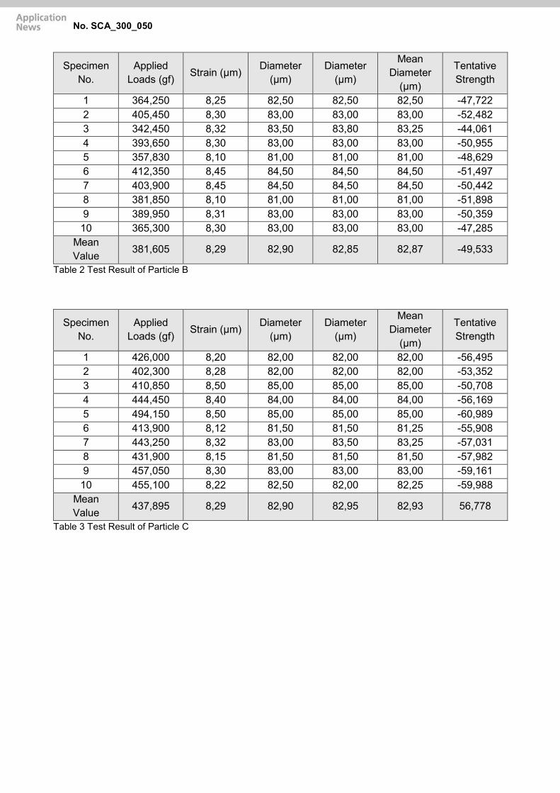
Specimen No.
Applied Loads (gf) Strain (µm) Diameter
(µm) Diameter
(µm)
Mean Diameter
(µm)
Tentative Strength
1 364,250 8,25 82,50 82,50 82,50 -47,722 2 405,450 8,30 83,00 83,00 83,00 -52,482 3 342,450 8,32 83,50 83,80 83,25 -44,061 4 393,650 8,30 83,00 83,00 83,00 -50,955 5 357,830 8,10 81,00 81,00 81,00 -48,629 6 412,350 8,45 84,50 84,50 84,50 -51,497 7 403,900 8,45 84,50 84,50 84,50 -50,442 8 381,850 8,10 81,00 81,00 81,00 -51,898 9 389,950 8,31 83,00 83,00 83,00 -50,359 10 365,300 8,30 83,00 83,00 83,00 -47,285
Mean Value 381,605 8,29 82,90 82,85 82,87 -49,533
Table 2 Test Result of Particle B
Specimen No.
Applied Loads (gf) Strain (µm) Diameter
(µm) Diameter
(µm)
Mean Diameter
(µm)
Tentative Strength
1 426,000 8,20 82,00 82,00 82,00 -56,495 2 402,300 8,28 82,00 82,00 82,00 -53,352 3 410,850 8,50 85,00 85,00 85,00 -50,708 4 444,450 8,40 84,00 84,00 84,00 -56,169 5 494,150 8,50 85,00 85,00 85,00 -60,989 6 413,900 8,12 81,50 81,50 81,25 -55,908 7 443,250 8,32 83,00 83,50 83,25 -57,031 8 431,900 8,15 81,50 81,50 81,50 -57,982 9 457,050 8,30 83,00 83,00 83,00 -59,161 10 455,100 8,22 82,50 82,00 82,25 -59,988
Mean Value 437,895 8,29 82,90 82,95 82,93 56,778
Table 3 Test Result of Particle C
No. SCA_300_050

Fig. 2 Load- Strain Curve for Particle A
Fig. 3 Load- Strain Curve for Particle B
Fig. 4 Load- Strain Curve for Particle C
Kinds of Specimen
Compression Test Hardness
Test Tensile
Strength (kgf/mm2)
Standard Deviation (kgf/mm2)
HRC 2)
A 31.36 3.00 34 B 49.53 2.60 52 C 56.78 3.07 57
Table 4 summary of the test results
■ Test Conditions
Sample No 1
Test 5
Indenter Vickers Flat
Read Time 2
Load 100 g
Loading Time 15 sec
No. SCA_300_050

Kinds of Specimen A B C
Test 1 1 1 D1 23,3 18,4 17,0 D2 23,4 18,1 16,8 HV 339 555 648
Test 2 2 2 D1 23,6 18,7 16,8 D2 23,3 18,3 17,2 HV 336 541 640
Test 3 3 3 D1 23,0 18,5 17,2 D2 23,2 18,2 17,0 HV 347 535 633
Test 4 4 4 D1 23,7 18,8 17,1 D2 23,6 18,4 16,7 HV 331 535 648
Test 5 5 5 D1 23,5 18,5 17,0 D2 23,8 18,7 17,2 HV 331 535 633
Average HV 337 543 640
Min HV 331 535 633 Max HV 347 555 648
Table 5 Result of Vickers Hardness
■ Comment on test results Table 4 shows a summary of the test results, while Tables 1 through 3 and Figs. 2 through 4 present measured data. Figs. 2 through 4 show examples of load-strain curves for each kind of specimen having the same diameter. Vickers Hardness Indexes are shown in Table 5 for each respective particle specimen. Table 4 indicates the correlation between tensile strength and Rockwell Hardness. Figs. 2 through 4 indicate that the order of strain size at a given load shows the same trend as that of hardness. According to these results, hardness decreases as strain increases, and increases as strain decreases.
No. SCA_300_050

■ Introduction One advance in metallurgy is the recent development in forming technology for the production of metal powders composed of microspherical particles ranging in size from several μm to 100μm. Evaluation of the mechanical properties of these particles as individual microspheres and as aggregates is required. The MCTM was applied to compression strength testing of Al-Ni alloy microspheres subjected to various heat treatments, and dependence of compression strength on the treatment temperature was observed.
The Model MCTM applies a pressing load of electromagnetic force at a constantly increasing rate onto a specimen placed between an upper pressing indenter and a lower anvil for automatic measurement of deforming behavior of the specimen and data processing for its relation to load. This testing machine is optimized for evaluating the physical strength of various micro-scale parts, powders and fine particle bodies, micro fibers, etc.
■ Specimens 1) Material name Al-Ni type alloy
2) Kinds
Three different heat treatments • no heat treatment, • 200 °C heat treatment, • 400 °C heat treatment
3) Shape micro sphere
■ Testing conditions 1) Testing mode compression test 2) Upper pressing indenter flat, diameter 50μmD(diamond) 3) Lower platen SKS flat plate
4) Strength calculation
A 10% strength was calculated from the load value and particle diameter when strain reached 10% of particle diameter with the following equation, as the three specimens did not reach the state of breakage or fracture. The values hereby obtained are shown on the data sheet as tentative strength with a minus sign (-) to discriminate from fracture strength.
Material Testing System MCT
Compressive Strength of Metallic Microspheres and Dependence on Heat Treatment Temperature. Shimadzu MCTM-500 Micro Compression Testing Machine No. SCA_300_061

(Quoted from the equation by Hiramatsu, et al.)
𝑆𝑆𝑆𝑆𝑆𝑆𝑆𝑆 =2,8 ∙ 𝑃𝑃𝑃𝑃𝜋𝜋𝜋𝜋 ∙ 𝑑𝑑𝑑𝑑2
St: tensile strength (kgf/mm2)
P: Load (kgf)
d: Diameter of particle (mm)
Note: Mr. Hiramatsu, Mr. Oka, Mr. Kiyama, Mining Association Journals
If particle diameter is 6,7 µm, strength is calculated with a load of 1,085 gf (P1) at a compression displacement of 0,67 mm (D1)
S10=21,553 kgf/mm2)
Fig. 1 Load-Displacement Curve
No. SCA_300_061

Table 1 Test results for untreated sample
Testing Conditions
File No. AN408.D1 Test mode 1 Indenter: Flate plate 50 Sample name Aluminium-Nickel alloy Sample No. 4
Testing load 100.00 (gf) Loading rate constant: 1
Displacement scale 10 (µm)
No. Load
(gf) Displacement
(µm) Diameter
(µm) Diameter
(µm) Average
(µm) Strength (kgf/mm2)
Tentative strength
1 1.085 0.67 6.70 6.70 6.70 -21.553 2 1.335 0.75 7.40 7.30 7.35 -22.036 3 6.480 1.49 15.00 14.90 14.95 -25.854 4 6.765 1.53 15.20 15.40 15.30 -25770 5 11.860 1.88 18.90 18.70 18.80 -29.922 6 14.320 1.90 19.00 19.00 19.00 -35.372 7 13.430 1.92 19.20 19.20 19.20 -32.486 8 19.125 2.14 21.50 21.40 21.45 -37.066 9 20.860 2.18 21.90 21.80 21.85 -38.962
10 29.785 2.59 25.90 25.90 25.90 -39.594 11 27.975 2.71 27.10 27.10 27.10 -33.967 12 31.035 3.05 30.60 30.50 30.55 -29.652 13 36.040 3.35 33.50 33.50 33.50 -28.637 14 49.100 3.94 39.20 39.20 39.20 -28.493 15 61.400 4.46 44.60 44.70 44.65 -27.463
Average ----- ----- 23.05 23.02 23.03 Average 22.040 2.30 ----- -30.455
Fig. 2 10%Strentgh - Particle Diameter plot for untreated sample
No. SCA_300_061

Table 2 Test results for treated sample at 200 °C
Testing Conditions
File No. 4-200.D2 Test mode 1 Indenter: Flate plate 50 Sample name Aluminium-Nickel alloy Sample No. 4-200
Testing load 100.00 (gf) Loading rate constant: 1
Displacement scale 10 (µm)
No. Load
(gf) Displacement
(µm) Diameter
(µm) Diameter
(µm) Average
(µm) Strength (kgf/mm2)
Tentative strength
1 1.580 0.65 6.30 6.30 6.45 -33.866 2 2.390 0.78 7.90 7.90 7.85 -34.585 3 4.705 1.12 11.20 11.20 11.20 -33.447 4 6.400 1.25 12.50 12.40 12.45 -36.819 5 12.515 1.67 16.70 16.70 16.70 -40.015 6 13.885 1.80 18.00 18.00 18.00 -38.215 7 15.235 1.83 18.20 18.40 18.30 -40.567 8 20.010 2.07 20.80 20.70 20.75 -41.442 9 23.460 2.26 22.60 22.70 22.65 -40.777
10 29.380 2.54 25.40 25.40 25.40 -40.608 11 34.765 2.85 28.80 28.30 28.55 -38.033 12 43.475 3.42 34.20 34.30 34.25 -33.048 13 43.970 3.81 38.20 38.00 38.10 -27.011 14 49.555 4.13 41.30 41.30 41.30 -25.907 15 46.455 4.16 41.60 41.70 41.65 -23.875
Average ----- ----- 22.91 22.90 22.91 Average 23.185 2.29 ----- -35.214
Fig. 3 10%Strentgh - Particle Diameter plot for sample treated at 200 °C
No. SCA_300_061

Table 3 Test results for treated sample at 400 °C
Testing Conditions
File No. 4-200.D3 Test mode 1 Indenter: Flate plate 50 Sample name Aluminium-Nickel alloy Sample No. 4-400
Testing load 100.00 (gf) Loading rate constant: 1
Displacement scale 10 (µm)
No. Load
(gf) Displacement
(µm) Diameter
(µm) Diameter
(µm) Average
(µm) Strength (kgf/mm2)
Tentative strength
1 1.170 0.68 6.80 6.90 6.85 -22.235 2 1.655 0.83 8.20 8.20 8.20 -21.948 3 3.205 1.11 11.00 11.00 11.00 -23.620 4 5.145 1.35 13.60 13.40 13.50 -25.174 5 7.000 1.54 15.40 15.40 15.40 -26.320 6 9.880 1.91 19.20 19.00 19.10 -24.150 7 10.945 1.99 19.90 20.00 19.95 -24.522 8 12.190 2.10 21.00 21.00 21.00 -24.649 9 14.170 2.26 22.60 22.70 22.65 -24.630
10 18.190 2.73 27.40 27.20 27.30 -21.764 11 22.520 3.00 30.10 29.90 30.00 -22.313 12 24.550 3.11 31.10 31.20 31.15 -22.561 13 34.590 3.73 37.30 37.40 37.75 -22.110 14 44.200 4.06 40.60 40.60 40.60 -23.911 15 41.850 4.30 43.80 42.20 43.00 -20.183
42.20 ----- ----- 23.20 23.07 23.14 23.07 16.751 2.31 ----- -23.339
Fig. 4 10%Strentgh - Particle Diameter plot for sample treated at 400 °C
■ Test results
Measured data are given in Tables 1 - 3 and Figs. 2 - 4.
No. SCA_300_061

Figs. 2 through 4 display 10% strength - particle diameter plots. The strength of the sample without heat treatment abruptly rises to approx. 40 kgf/mm2 at a particle diameter of around 25 μm, as shown in Fig. 2. Compared with the specimen without heat treatment, the specimen with heat treatment at 200 °C has a
high level of strength at 35 to 40 kgf/mm2 in the lower particle diameter range (below 20 μm). The strength of the sample with heat treatment at 400 °C remains at a low level of around 25 kgf/mm2 without any significant variation across diameters. As shown above, this data provides much information about the difference of strength depending on diameter size or method of heat treatment.
* Please be advised that data obtained before the implementation of the current Weights and Measures Law may be presented in terms of gravimetric unit.

ApplicationNews
No.V21
High-Speed Video Camera
Observation of Bending Fatigue Testing of Metal Plate at Ultrasonic Frequency
LAAN-A-HV-E006
High-speed video camera : HPV-X2
Microscope : Z16 APO
Lighting : Strobe
Testing apparatus : USF-2000
Measurement speed : 2 million frames/secTest frequency : 20 kHzTest specimen size : 10.0 × 3.020 × 0.406 mm
Testing site
1st Order
3rd Order
2nd Order
HPV-X2Strobe
HornMicroscope
Horn
Microscope
Test Specimen
n Introduction
n Measurement System
Fig. 1 Specimen
Fig. 2 Bending Mode Examples
Fig. 3 Overview of Test
Fig. 4 Periphery of Specimen
Table 1 Imaging Equipment
Table 2 Measurement Conditions
Fatigue failure refers to the fracture of a component due to repeated load cycles, which can occur using a force much smaller than the static fracture strength. Also, because fatigue-related failure occurs suddenly, there are cases where this has led to serious accidents involving ships and aircraft. Therefore, knowledge of the fatigue propert ies of mater ials used in products is very important . However, determinat ion of fat igue characteristics typically requires time-consuming testing using 107 repetitions (as per JIS Z2273, General Rules for Fatigue Testing of Metals), which at 10 Hz, takes about 12 days to complete. Also, due to enhancements in equipment efficiency and speed, there are now requests for fatigue evaluation with more than 107 repetitions. In response to this, an ultrasonic testing machine capable of 20 kHz ultrasonic fatigue testing is now in use. However, due to the very rapid vibration that is generated during measurement with this instrument, visual confirmation of the movement and deformation of the specimen is not possible. Therefore, a high-speed video camera was used to observe the movement of a metal plate vibrating while conducting a 20 kHz bending fatigue test. Previously, gaining an understanding of the overal l movement of the test specimen required incremental repositioning of a displacement gauge, but with the high-speed video camera, it is possible to evaluate the movement of the specimen in a single observat ion process. Further, the poss ib i l i ty of determining the amount of movement of the specimen from captured images was also demonstrated.
The USF-2000 Ultrasonic Fatigue Testing System and the HPV-X2 high-speed video camera were used for this experiment. Table 1 lists all the instrumentation that was used. Shooting during the test can be conducted at any desired timing. Fig. 1 shows a photograph of the test specimen. For the bending vibration, the vibration modes shown in Fig. 2 are available, with a test specimen dimensioned to resonate for each vibration mode. Here, a test specimen was prepared to provide a second-order bending mode.

ApplicationNews
No.
For Research Use Only. Not for use in diagnostic procedures.The content of this publication shall not be reproduced, altered or sold for any commercial purpose without the written approval of Shimadzu. The information contained herein is provided to you "as is" without warranty of any kind including without limitation warranties as to its accuracy or completeness. Shimadzu does not assume any responsibility or liability for any damage, whether direct or indirect, relating to the use of this publication. This publication is based upon the information available to Shimadzu on or before the date of publication, and subject to change without notice.
© Shimadzu Corporation, 2015www.shimadzu.com/an/
V21
First Edition: Sep. 2015
-100
100
80
60
40
20
0
-20
-40
-60
-80Am
ount
of
Mov
emen
t [µ
m]
0 20 40 60 80 100 120 140
Time [µsec]
① ② ③ ④
⑤ ⑥ ⑦ ⑧
⑨ ⑩ ⑪ ⑫
n Measurement Results n Conclusion
Fig. 6 Amount of Movement of Specimen
Fig. 5 High-Speed Images (Imaging interval: 5 µsec)
Fig. 3 shows an overview of the test setup, and Fig. 4 shows a close-up view of the vicinity of the specimen. The vibration generated by the actuator is amplified by the horn, causing the specimen to vibrate. Table 2 shows the measurement conditions. To obtain image data at more than 100 frames per cycle, the shooting speed must be set to two million frames/sec. Fig. 5 shows a series of captured images. The blue line traversing the images in Fig. 5 is situated at the center of the specimen in image (1). The central portion of the specimen is shifted in the downward direction as the images proceed from (1) to (3). Then, the center portion of the specimen shifts in the upward direction, reaching a maximum at image (9). From image (9), the specimen center descends once again, returning at image (11) to the same position as in image (1). From the above, the vibration cycle of the specimen was determined to be 20 kHz. Also, from Fig. 5, the specimen tip does not move very much, although it can be seen that the specimen is in a second-order bending mode due to movement of the test specimen center. Applying image processing software to the captured images permits determinat ion of the range of movement of the test specimen. Here, we determined the amount of movement of the central part of the specimen. Fig. 6 shows the relationship between time and the amount of movement of the specimen center. Also, from Fig. 6, the amplitude in the bending test is determined to be about 80 µm, and the vibration frequency is determined to be 20 kHz.
Fatigue testing of a target component conducted using the ultrasonic frequency was documented using the HPV-X2, and the movement characteristics of the test specimens were confirmed. The HPV-X2 proved to be effective in capturing the high-speed movement generated during the test, and installation of a microscope permitted visual documentation of these minute movements. Aside from this confirmation of movement in the specimen during the test, the actual degree of movement in the test specimen can be determined from the captured images. The USF-2000 calculates the stress amplitude from the amplitude of vibration, thereby permitting the determination of the stress load on the test specimen from the images. Thus, the HPV-X2 can effectively serve in the very important fatigue testing process during product development.

7. Railroad Industry

7. Railroad Industry
DEVELOPMENT OF THE RAILROAD INDUSTRY
Railroads have a long history as both a day-to-day means of transport for people, and a means of transporting freight over land. Railroad technology has made huge strides, changing its power source and component members in response to the desire to travel farther, faster and in more comfort, for lower cost and in a way that is better for the passengers.
Railroad technology has achieved superior levels of safety, comfort, speed, accuracy and energy savings. Gaining of these levels has required a wide range of evaluation testing. Such technical innovation is never-ending, and continues to increase in scale.
Evaluation instruments have also made similar strides. They are routinely used in the evaluation of physical characteristics in materials development as well as for quality control of com-ponents. Furthermore, they are applied in performance
evaluation of actual cars as well as reliability evaluation for infrastructure used in the operation of the railroads, and they continue to play a part in the assessment of a range of aspects of railroad development and operation.
Shimadzu has acquired a wealth of technical ability in regard to strength and endurance testing in the development of a range of materials and simulation testing on the actual sam-ple, and is actively engaged in applying this knowledge in the railroad industry.
Shimadzu provides solutions for evaluation of safety and com-fort during travel, e.g. through chassis tests as well as wheels and axles endurance evaluation. In addition, the company evaluates endurance and reliability of the track through ultra-sonic flaw detection or rail fatigue lifespan test.

7. Railroad Industry
C225-E032 Ultrasonic fatigue testing system with an average stress loading mechanism
C225-E033 Three-axis endurance evaluations of automobile steering mechanisms

C225-E032
Ultrasonic Fatigue Testing System Effective for Gigacycle Fatigue Tests
With fatigue tests of high-strength steels, it is evident that internal fracture (fish-eye fracture), which is caused by inclusions and other micro defects, occurs at 107 cycles or more, a value considered the conventional fatigue limit.An ultrasonic fatigue testing system is extremely effective when performing this sort of gigacycle fatigue test. (With a 100 Hz fatigue testing system, this would take 3 years, but if a 20 kHz ultrasonic fatigue testing system is used, testing can be completed in one week.)
Actual components are rarely used under conditions in which the average stress is zero. Despite this, the USF-2000A, a standard ultrasonic fatigue testing system, can only perform testing under zero average stress conditions.Using an ultrasonic fatigue testing system equipped with an average stress loading mechanism, gigacycle fatigue tests can be performed with average tensile stress loaded.
Ultrasonic Fatigue Testing System with an Average Stress Loading Mechanism
Stressdistribution
AG-X5kNAverage stress loading
High-rigidity booster
Horns
High-rigidity booster
5 kN load cellAverage stress measurement
Converter(Piezo actuator)
Strain GaugeSamples
DisplacementStress
System Appearance
For Gigacycle Fatigue Tests with Average Stress Loaded

© Shimadzu Corporation, 2016First Edition: August 2016
For Research Use Only. Not for use in diagnostic procedure. This publication may contain references to products that are not available in your country. Please contact us to check the availability of these products in your country.Company names, product/service names and logos used in this publication are trademarks and trade names of Shimadzu Corporation or its affiliates, whether or not they are used with trademark symbol “TM” or “®”. Third-party trademarks and trade names may be used in this publication to refer to either the entities or their products/services. Shimadzu disclaims any proprietary interest in trademarks and trade names other than its own.
The contents of this publication are provided to you “as is” without warranty of any kind, and are subject to change without notice. Shimadzu does not assume any responsibility or liability for any damage, whether direct or indirect, relating to the use of this publication.www.shimadzu.com/an/
Ultrasonic resonance systemPower supply, converter, booster (1 pair), horn (1 pair)
Personal computer(OS Windows 7) ADA/PIO interface board
SoftwareUltrasonic test control measurement software
Cooling systemAir dryer, air piping• A separate 140 L/min air source is required.
5 Strain meter unit (option)
6 AG-X plus Autograph 5 kN + 250 extension
7 Average stress loading mechanism
1
2
3
4
Main Speci�cations
1) Test Frequency: 20 kHz ± 500 Hz
• The recommended test range is 20 kHz ± 30 Hz.• The test frequency is determined by the resonance frequency of the sample.
2) Horn End Face Amplitude
Min. approx. ±10 μmMax. approx. ±50 μm
• The minimum and maximum amplitudes are the end face amplitude values at amplitude outputs of 20 % and 100 % respectively. Accordingly, the minimum and maximum amplitude values will change somewhat depending on the shape of the sample.
4) Average Stress
Max. 1.5 kN (tensile only)
3) Test Stress
Standard circular tapered sampleStress Min. 237 MPa Max. 1186 MPa• The test stress range can be changed by changing the sample shape.• The minimum and maximum values are calculated with the end face amplitude values of 10 μm and 50 μm respectively.• These are the values when the stress is within the elasticity range.
Standard Circular Tapered Sample
Surface of the Fatigued Fracture Originating from the Inclusion
Center hole can remain
Center holecan remain
Components

Steering mechanism unit
System Appearance
Automobile steering units are important components that must be highly durable. There are also significant differences in driver arm strengths, so many cars are equipped with a power steering mechanism, which complicates the structure. In contrast, with luxury cars and sports cars, specifications are required that can achieve an operable feeling that heightens the sense of enhanced value. In regards to these new and diversified requirements, quantitation, not only evaluations by people, is increasingly needed. By combining three actuators with the 4830 controller, which is capable of high-accuracy control, this system can easily perform endurance tests under close to real conditions.
1 Steering unit
3 Left tire unit
2 Right tire unit
Evaluation Details
■ Endurance tests in which the steering wheel is moved left and right more than one million times■ Endurance tests in which excessive force is applied to turn the steering wheel to the left or the right■ Quantitation of the sense of enhanced value (Rotational torque and angle of 1 and test force at 2 and 3 at each rotation point)
Steering mechanism unit
Three-Axis Endurance Evaluations ofAutomobile Steering MechanismsWith Control via Actual Data, Endurance Evaluations ApproximatingReal Motion Can Easily Be Performed
3 Left tire unit2 Right tire unit
1 Steering unit
Endurance tests of the steering mechanism unit are performed by adding a rotational force via the steering wheel 1 , and producing a reaction force originating from the tires in 2 and 3 .
The reaction force from 2 and 3 corresponding to the rotational angle in 1 is obtained for use from an actual car.
C225-E033

4830 Controller
Main Specifications
Left/Right Tire Units 1) Rated capacity: ±10 kN stroke ±100 mm
(static maximum load capacity ±13 kN)
2) With trunnion pin
3) Maximum speed: 500 mm/sec
(20 L/min hydraulic source, when unloaded)
Lifting Stand(For the left/right tire units)
1) Height: 300 mm to 800 mm
(electric lift, manual bolt fastening)
2) Angle: top/bottom ±10°
(can change fastened or mobile) and horizontal ±10°
Steering Unit 1) Rated capacity: ±200 Nm, Angle: ±1080 deg
2) Maximum speed: 360 deg/sec
3) Excitation frequency: 0.01 Hz to 2 Hz (±5 deg or more)
Lifting Stand(For the steering unit)
1) Height: 800 mm to 1200 mm (electric lift, manual bolt fastening)
2) Angle: top/bottom 0° to 60° (can change fastened or mobile)
Data Processing Example (PC Screen) The left window shows the data chart results when
the steering unit is turned to the left and right from
the center position, and then returns to the center.
The window on the left shows a chart of angle versus test force.
The window on the right shows a chart of time versus test force.
The blue line is the test force for the right tire unit.
The red line is the test force for the left tire unit.
© Shimadzu Corporation, 2016First Edition: August 2016

8. Plastics and Rubber Industry

Testing, Weighing and Analytical Instruments For Rubber and Plastics
8. Plastics and Rubber Industry
EVALUATION OF RUBBER AND PLASTICS
Rubber and plastic products are used in a wide variety of industrial areas such as packaging, construction, automotive, electronics, furniture, household goods, agriculture and medi-cal. Plastomers, thermosetting plastic and elastomer materials are commonly used in various applications. Physical properties determine their important features, e.g. lightweight, hardness, density, resistance to heat, flexibility, moldability and chemi-cal resistance.
Plastics and rubber are growing industries, and they are pro-duced worldwide. They are also part of the supply chain in many industries. Evaluation of their basic performance and
determined components is indispensable to product develop-ment and quality control. Applications include evaluation of rheological, thermal, statical and dynamic strength properties of additives and harmful materials as well as observation and measurement.
Shimadzu not only offers a wide array of evaluation instru-ments, but also provides comprehensive support from applica-tion to after-sales service. On the following pages are over 30 applications covering most versatile cases of material testing and inspection.

8. Plastics and Rubber Industry
C225-E034 System to test fatigue and endurance of rubber in clean environment
No.1 Tensile test of various plastic materials
No.2 Flexural test of plastic ISO178
No.3 Tensile tests of plastic materials at low ISO527 1
No.4 Tensile test of rubber dumb bell specimens ISO37
No.5 Tear test of crescent shaped ISO34 1
No.6 Tear tests of angle shaped rubber specimens ISO34 1
No.7 Tensile tests of films ISO527 3
No.9 Measurements of modulus of elasticity and poisson’s ratio for films ISO527
No.17 Measurement of friction coefficient of film
No.18 90 degree peel resistance test of adhesive tape
No.19 180 degree peel resistance test of adhesive tape
No.20 Measurement of friction coefficient of film
No_05 Fluidity evaluation of unvulcanized rubber
No_06 Evaluation of the temperature characteris-tics of general plastics
No_07 CFT EX useful to evaluation of LED package
No_08 Why is CFT used to evaluate thermosetting resins
No_09 Fluidity evaluation of epoxy resin
No_10 Fluidity evaluation of ic sealant
SCA_300_010 Endurance testing and dynamic visco- elasticity measurement of EVA Film by MMT-100N
SCA_300_013 Evaluation of mooney viscosity by Shimadzu mooney viscometer, model SMV
SCA_300_014 Evaluation of surface hardness of audio-tapes with Shimadzu dynamic ultra micro hardness tester model DUH
SCA_300_017 Flow tests of various kinds of plastics with Shimadzu flowtester model CFT
SCA_300_021 Hardness measurement of plastic tubes using the Shimadzu dynamic ultra micro hardness tester DUH
SCA_300_026 Measurement of surface hardness of eras-ers with Shimadzu dynamic ultra micro hardness tester
SCA_300_028 Measuring and controlling performance of Shimadzu mooney viscometer model SMV in viscosity tests on rubber materials
SCA_300_031 Test on thermosetting resin with Shimadzu flow tester model CFT
No.ei253 Tensile test of plastic materials
No.ei249 Three-point bending flexural test of plastics (ISO178, JIS K 7171)
SCA_300_038 Deformation of rubber vibration isolators
SCA_300_039 Evaluation of elastic recovery in hardness measurement of plastic materials with Shimadzu dynamic ultra micro hardness tester
SCA_300_043 Fluidity evaluation of unvulcanized rubber
SCA_300_054 Viscosity evaluation of thermoplastic resins (epoxies)
SCA_300_057 Breaking strain measurement of ABS resin


0 10 20 30 40 500
10
20
30
40
50
60
70
80
PC
PP
応力
(MP
a)
ひずみ(%)
PVC


曲げひずみ
曲げ応
力


ひずみ
応力


変位
試験
力


変位
試験
力


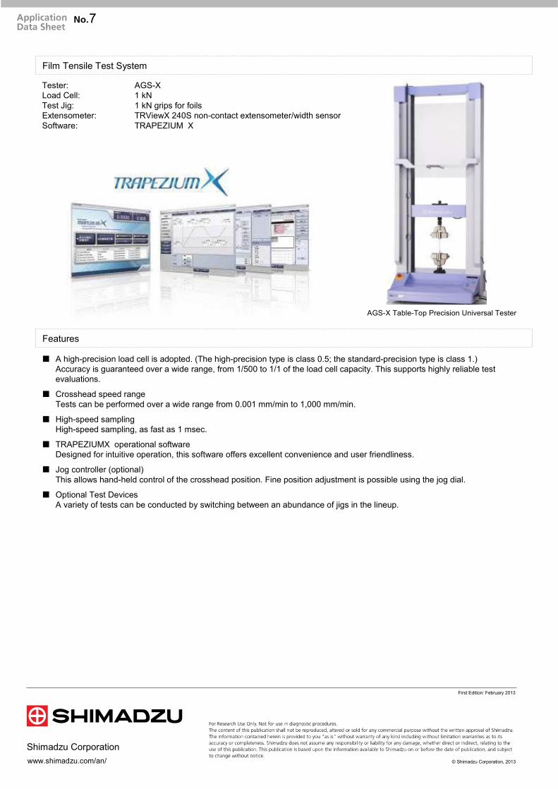
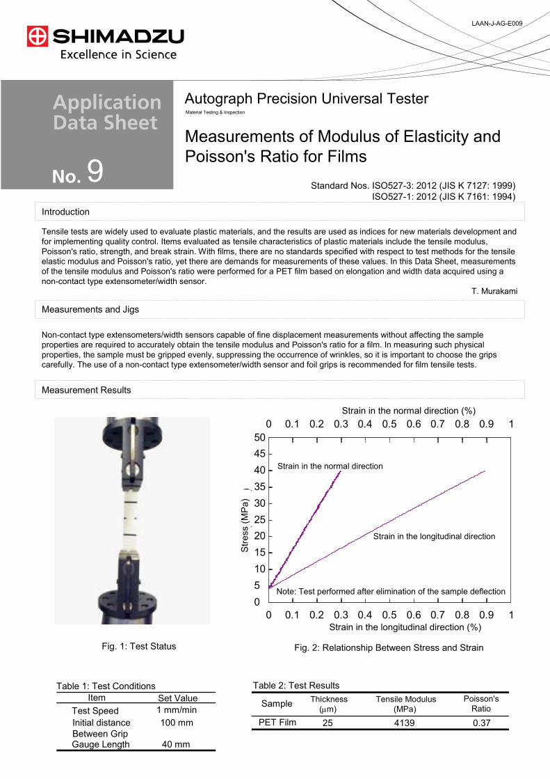
縦ひずみ
横ひずみ
応力


17
LAAN-J-AG0017
Material Testing & Inspection
Autograph Precision Universal Tester
Introduction
Plastic films are used for coating or wrapping of various materials. It is often necessary to measure sliding friction between two films or between a film and a different material. For example, the coefficient of friction of film for foods and that of protection film for smartphones are measured. In this Application Data Sheet, measurement examples of the static and dynamic coefficients of friction for polyethylene film in accordance with the ISO standard are introduced.
F. Yano
Measurement and Jigs
Measurement Results
Standard No. ISO 8295: 1995 (JIS K 7125: 1999)
The standard specifies the method of measuring the coefficients of starting and sliding friction of plastic films and sheets. This method measures the coefficient of friction of plastic films and sheets that are not sticky up to 0.5 mm thickness. The test requires 2 test specimens of size about 80 mm 200 mm, and the test apparatus generally includes a horizontal testing table, a sliding member, and a drive mechanism that produces relative motion between the test table and the sliding member. In these tests, the AGS-X Table-Top Precision Universal Tester and friction coefficient measuring apparatus were used to evaluate polyethylene film.
Item Set Value
Test speedLoad cell capacity
100 mm/min5 N
Table 1 Test Conditions
Static Coefficient of Friction
Dynamic Coefficient of Friction
0.23 0.19
Table 2 Test Results
Fig. 1 Test Status
Reinforced plate
Film Sliding member(200 2 g)
Measurement of Friction Coefficient of Film
Fig.2 Test Results
ストローク [mm]
試験力
[N]
Test
forc
e (N
)
Stroke (mm)

17
First Edition: February 2013
© Shimadzu Corporation, 2013www.shimadzu.com/an/
Shimadzu Corporation
AGS-X Table-Top Precision Universal Tester
A high-precision load cell is adopted. (The high-precision type is class 0.5; the standard-precision type is class 1.)Accuracy is guaranteed over a wide range, from 1/500 to 1/1 of the load cell capacity. This supports highly reliable test evaluations.
Cross head speed rangeTest can be performed over a wide range from 0.001 mm/min to 1,000 mm/min.
High speed samplingHigh speed sampling, as fast as 1 msec.
TRAPEZIUMX LITE X operational softwareThis is simple, highly effective software.
Jog controller (optional)This allows hand-held control of the crosshead position. Fine position adjustment is possible using the jog dial.
Optional Test DevicesA variety of tests can be accommodated by switching between an abundance of jigs in the lineup.
Features
Friction Coefficient Measurement System
Tester: AGS-XLoad Cell: 5 NTest Jig: Friction coefficient measuring apparatusSoftware: TRAPEZIUM LITE X

18
LAAN-J-AG0018
Material Testing & Inspection
Autograph Precision Universal Tester
Measurement Results
Fig. 1 Test Status Fig. 2 Relationship Between Test Force and Stroke
General adhesive tape cut to a width of 24 mm and length of 300 mm was used as the test sample, and a SUS304 stainless steel plate was used as the test plate for setting the sample. An adhesive tape peel resistance test apparatus that was capable of peeling the sample at a constant 90 degree to the test plate was used.
Adhesives are widely used in many industrial fields such as electronics and electrical machinery. Starting from the use of materials such as glue to join solids together, adhesives that use synthetic polymers as the raw material have been commercialized with the progress of the chemical industry. In this Application Data Sheet, examples of the 90-degree peeling test for adhesive material used for adhesive tape are introduced.
T. Murakami
Measurement and Jigs
Introduction
Sandard No. ISO29862: 2007 (JIS Z 0237 :2009)
The tests were carried out at a load rate of 300 mm/min. The measured values for the initial 25 mm length after start of testing were ignored, and the subsequent adhesion force measurement values for subsequent 50 mm length peeled from the test plate were averaged to obtain the peel adhesion force.
90-Degree Peel Resistance Test of Adhesive Tape
Test
forc
e (N
)
Stroke (mm)
Table 1 Test Results
Peel Adhesion Force 0.238 N/10 mm

18
First Edition: February 2013
© Shimadzu Corporation, 2013www.shimadzu.com/an/
Shimadzu Corporation
AGS-X Table-Top Precision Universal Tester
A high-precision load cell is adopted. (The high-precision type is class 0.5; the standard-precision type is class 1.)Accuracy is guaranteed over a wide range, from 1/500 to 1/1 of the load cell capacity. This supports highly reliable test evaluations.
Cross head speed rangeTest can be performed over a wide range from 0.001 mm/min to 1,000 mm/min.
High speed samplingHigh speed sampling, as fast as 1 msec.
TRAPEZIUMX LITE X operational softwareThis is simple, highly effective software.
Jog controller (optional)This allows hand-held control of the crosshead position. Fine position adjustment is possible using the jog dial.
Optional Test DevicesA variety of tests can be accommodated by switching between an abundance of jigs in the lineup.
Features
Tester: AGS-XLoad Cell: 50 NTest Jig: Adhesive tape peel resistance test apparatusSoftware: TRAPEZIUM LITE X
Plastic Material Tensile Test System

19
LAAN-J-AG0019
Material Testing & Inspection
Autograph Precision Universal Tester
Sandard No. ISO29862: 2007 (JIS Z 0237 :2009)
Measurement Results
Adhesives are widely used in many industrial fields such as electronics and electrical machinery. Starting from the use of materials such as glue to join solids together, adhesives that use synthetic polymers as the raw material have been commercialized with the progress of the chemical industry. In this Application Data Sheet, examples of the 180-degree peeling test for adhesive material used for adhesive tape are introduced.
T.Murakami
Introduction
The tests were carried out at a load rate of 300 mm/min. The measured values for the initial 25 mm length after start of testing were ignored, and the subsequent adhesion force measurement values for subsequent 50 mm length peeled from the test plate were averaged to obtain the peel adhesion force.
Fig. 1 Test Status
Measurement and Jigs
General adhesive tape cut to a width of 24 mm and length of 300 mm was used as the test sample, and a SUS304 stainless steel plate was used as the test plate for setting the sample. When the sample was peeled, the ends of the tape were held and folded through 180 degree so that the back of the tape was overlapped. After the sample was peeled 25 mm from the test plate, one end of the test plate from which the tape had been peeled was fixed in the lower jig set in the testing machine, and the adhesive tape was fixed in the upper jig.
180-Degree Peel Resistance Test of Adhesive Tape
Fig. 2 Relationship Between Test Force and Stroke
Test
forc
e (N
)
Stroke (mm)
Table 1 Test Results
Peel Adhesion Force 0.217 N/10 mm

19
First Edition: February 2013
© Shimadzu Corporation, 2013www.shimadzu.com/an/
Shimadzu Corporation
AGS-X Table-Top Precision Universal Tester
A high-precision load cell is adopted. (The high-precision type is class 0.5; the standard-precision type is class 1.)Accuracy is guaranteed over a wide range, from 1/500 to 1/1 of the load cell capacity. This supports highly reliable test evaluations.
Cross head speed rangeTest can be performed over a wide range from 0.001 mm/min to 1,000 mm/min.
High speed samplingHigh speed sampling, as fast as 1 msec.
TRAPEZIUMX LITE X operational softwareThis is simple, highly effective software.
Jog controller (optional)This allows hand-held control of the crosshead position. Fine position adjustment is possible using the jog dial.
Optional Test DevicesA variety of tests can be accommodated by switching between an abundance of jigs in the lineup.
Features
Tester: AGS-XLoad Cell: 50 NTest Jig: 50 N pneumatic flat grips (plane teeth)Software: TRAPEZIUM LITE X
Plastic Material Tensile Test System

20
LAAN-J-AG0020
Material Testing & Inspection
Autograph Precision Universal Tester
Standard No. ASTM D 1894 - 95 (JIS K 7312 - 1996)
Introduction
Plastic films are used for coating or wrapping of various materials. It is often necessary to measure sliding friction between two films or between a film and a different material. For example, the coefficient of friction of film for foods and that of protection film for smartphones are measured. In this Application Data Sheet, measurement examples of the static and dynamic coefficients of friction for polyethylene film in accordance with the ASTM standard are introduced.
F. Yano
Measurement Results
Measurement and Jigs
The standard specifies the method of measuring the coefficients of starting and sliding friction of plastic films and sheets. These tests were carried out on polyethylene film using the AGS-X Table-Top Precision Universal Tester and friction coefficient measuring apparatus. Two test samples were prepared: a movable sample and a fixed sample. The measurements were carried out with the movable sample (a square test specimen of side 63.5 mm) fastened to a metal sled using double-sided tape, and the fixed sample (rectangular test specimen of width 130 mm and length 250 mm minimum) fastened to a platform using double-sided tape.
Item Set Value
Test speed Moving distance
Load cell capacity
150 mm/min130 mm
5 N
Table 1 Test Conditions
Static Coefficient of Friction
Dynamic Coefficient of Friction
0.21 0.17
Table 2 Test Results
Fig. 1 Test Status
Metal sled
Measurement of Friction Coefficient of Film
Fig.2 Test Results
ストローク [mm]
試験力
[N]
Test
forc
e (N
)
Stroke (mm)

20
First Edition: February 2013
© Shimadzu Corporation, 2013www.shimadzu.com/an/
Shimadzu Corporation
Friction Coefficient Measurement System
AGS-X Table-Top Precision Universal Tester
A high-precision load cell is adopted. (The high-precision type is class 0.5; the standard-precision type is class 1.)Accuracy is guaranteed over a wide range, from 1/500 to 1/1 of the load cell capacity. This supports highly reliable test evaluations.
Cross head speed rangeTest can be performed over a wide range from 0.001 mm/min to 1,000 mm/min.
High speed samplingHigh speed sampling, as fast as 1 msec.
TRAPEZIUMX LITE X operational softwareThis is simple, highly effective software.
Jog controller (optional)This allows hand-held control of the crosshead position. Fine position adjustment is possible using the jog dial.
Optional Test DevicesA variety of tests can be accommodated by switching between an abundance of jigs in the lineup.
Features
Tester: AGS-XLoad Cell: 5 NTest Jig: Friction coefficient measuring apparatusSoftware: TRAPEZIUM LITE X

Shimadzu Flowtester
CFT-EX Series Application Topic #05
Rubber products are produced by forming rubber compounds (mixtures of rubber and additives that provide specific functional characteristics) in a mold and then applying heat to provide an elastic body. Therefore, the fluidity of rubber compounds can have a major effect on molding quality. Unformed rubber compounds change their characteristics after long storage periods, which can cause fluidity to deteriorate or the molding process to fail, depending on how they are stored.
Here, the example which evaluated the fluidity change by the storage
method of the unvulcanized rubber is introduced.
Fluidity Evaluation of Unvulcanized Rubber
In this case, a rubber compound was stored at ambient temperature and low temperature for 14 days and 28 days immediately after kneading and then the fluidity was evaluated.
The results showed that the given sample could be stored at low temperatures without a significant change in fluidity, even after one month.
Using the CFT-EX series allows evaluating the rubber compounds storage temperatures and storage periods without actually having to mold any parts.
Fluidity Change by the Storage Method of Unvulcanized Rubber
280 ℃
0
100
200
300
400
500
600
700
0 5 10 15 20 25 30
Visc
osity
(Pa.
s)
Storage Period
常温
低温
Changes in Viscosity Due to Storage Methods
Ambient Temperature
Low Temperature

Shimadzu Flowtester
CFT-EX which can evaluate thermosetting and thermoplastic resin in evaluation of unvulcanized rubber is recommended.
CFT-EX can use evaluation of unvulcanized rubber
Higher Level Evaluation Using a Variety of Analysis Methods ・・・
Smooth, Easy Test Flow ・・・ ,
Supported by More Than 50 Years of Technology and Know-How ・・・
Thermosetting resins Thermoplastic resins
Toners
Composites
Rubbers
Ceramics
Thermosetting resinsThermoplastic resins
Toners
Composites
Rubbers
Ceramics
The fluidity of various materials
& Evaluation of the heat
characteristic
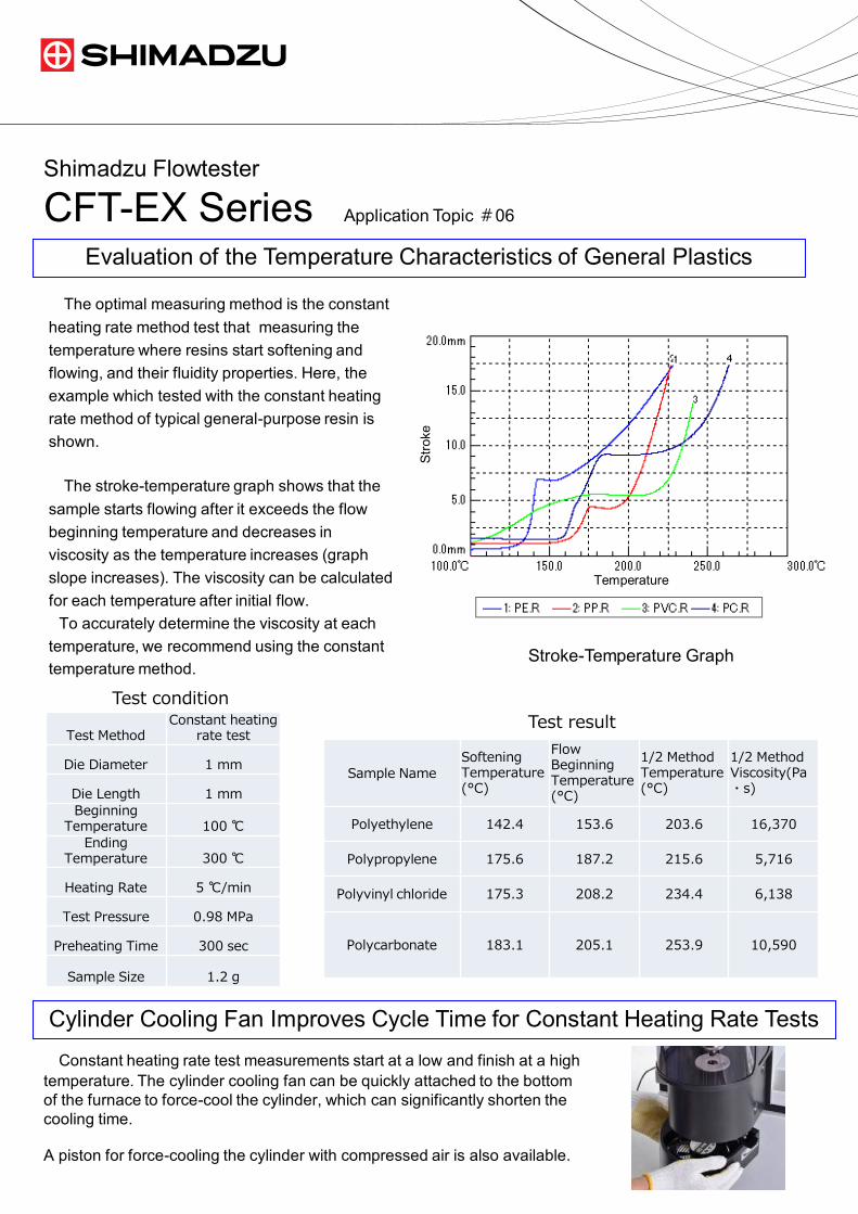
Shimadzu Flowtester
CFT-EX Series Application Topic #06
Constant heating rate test measurements start at a low and finish at a high temperature. The cylinder cooling fan can be quickly attached to the bottom of the furnace to force-cool the cylinder, which can significantly shorten the cooling time. A piston for force-cooling the cylinder with compressed air is also available.
Evaluation of the Temperature Characteristics of General Plastics
The optimal measuring method is the constant heating rate method test that measuring the temperature where resins start softening and flowing, and their fluidity properties. Here, the example which tested with the constant heating rate method of typical general-purpose resin is shown.
The stroke-temperature graph shows that the sample starts flowing after it exceeds the flow beginning temperature and decreases in viscosity as the temperature increases (graph slope increases). The viscosity can be calculated for each temperature after initial flow.
To accurately determine the viscosity at each temperature, we recommend using the constant temperature method.
Cylinder Cooling Fan Improves Cycle Time for Constant Heating Rate Tests
Stroke-Temperature Graph
° ° ° ・
℃
℃
℃
Temperature
Stro
ke

CFT-EX is recommended for evaluation of a general-purpose plastic because it can simply evaluated about the flow characteristic for the temperature of resin by the constant heating rate method.
CFT-EX can use evaluation of general plastic.
Shimadzu Flowtester
Higher Level Evaluation Using a Variety of Analysis Methods ・・・
Smooth, Easy Test Flow ・・・ ,
Supported by More Than 50 Years of Technology and Know-How ・・・
Thermosetting resins Thermoplastic resins
Toners
Composites
Rubbers
Ceramics
Thermosetting resinsThermoplastic resins
Toners
Composites
Rubbers
Ceramics
The fluidity of various materials
& Evaluation of the heat
characteristic

LEDs are used in various fields for their beneficial features such as long lifetime, low energy consumption, and small size. We often see LEDs in our everyday life since they are used in illuminations, traffic signals, lighting, backlights for LCD televisions, cellular phones, and car lights. To manufacture LEDs, electrode or other parts are attached on elements, wires are connected, and then the parts are sealed with resin for protection. This process is called packaging. In addition to more efficient elements, optimized packaging technology helps to draw light from LED elements efficiently and enhance light directionality.
The replacement from a filament lamp to white LED lighting is progressing because of the energy-saving, and the new product has come out one after another. One of the big features of LED lighting is a longer operating life (20,000 hours: filament lamp is 1,500 hours), and the major factor which influences the life is "heat." For this reason, the heat-resistant design and the heat dissipation design are important.
Therefore, the filler of a carbon system or a ceramic system is used for resin, or the material which made insulation and heat dissipation compatible by unification with a printed circuit board is developed, and the manufacturing cost reduction which includes a moldability as a metaled substitute article is proposed.
The moldability (fluidity) is an important item for evaluation of plastic new materials. CFT-EX is the optimal equipment at this evaluation.
Round LED Package Mounted LED Package
Sealing resin
LED element
Reflector
Resins used in LED packages have a lens-like function to focus light or a reflector-like function and also disperse phosphors for white LEDs. For the lens, thermoplastic resins such as transparent acrylic resin and polycarbonate resins are used. For resin material to mold LED elements, thermosetting resins such as epoxy resin and silicon resin are used. The optimum resin selection, higher functions, and more consistent quality are demanded for easier molding and higher adhesiveness with elements and other parts.
Recently, there has been a growing awareness about white LEDs which are expected to be applied to a wide range of products, from backlights for televisions to general lighting fixtures. (The global market of sealing materials for LEDs is estimated to grow to 22.7 billion yen in year 2013 which is approximately three times larger than the market size in 2008.) Mainstream white LEDs are currently created by combining blue diode and phosphor. White LEDs have a problem of shorter lifetime due to deterioration of packaging resins caused by heat along with higher luminance and deterioration caused by UV ray generated by luminance of phosphor. In order to solve these problems, there is a growing demand for higher heat resistance and UV-proof functions on packaging resins.
Shimadzu flowtester is an optimum system to evaluate these resins for packaging LEDs because fluidity properties and hardening properties (by heating test) can be measured easily and accurately.
Shimadzu Flowtester
CFT-EX Series Application Topic #07

CFT-EX which can evaluate thermosetting and thermoplastic resin in evaluation of the LED package for which various resin is used is recommended.
CFT-EX can use evaluation of LED
Shimadzu Flowtester
Higher Level Evaluation Using a Variety of Analysis Methods ・・・
Smooth, Easy Test Flow ・・・ ,
Supported by More Than 50 Years of Technology and Know-How ・・・
Thermosetting resins Thermoplastic resins
Toners
Composites
Rubbers
Ceramics
Thermosetting resinsThermoplastic resins
Toners
Composites
Rubbers
Ceramics
The fluidity of various materials
& Evaluation of the heat
characteristic

What is thermosetting resins? Resins are generally classified into thermoplastic resins and thermosetting resins. Similar to chocolate, thermoplastic resins soften and become deformed when heated.
They can be processed when they are soft and harden when cooled. They soften if heated again and can be used repeatedly. Major examples are polyethylene terephthalate (PET) used in PET bottles and polypropylene (PP) used in kitchen goods.
Why Is CFT Used to Evaluate Thermosetting Resins?
Phenol resin (PF) Automobile field: Engine-related parts, electric parts, disk pads, clutch facing, or other bonding materials Electric fields: Parts such as switches and breakers, power supply transformer bobbins Bonding material for grind stones Epoxy resin (EP) Cast products: Circuit units of AC transformers and open/close equipments Laminated products: Printed circuit boards, insulating boards Molded products: Packaging and connectors of electronic parts such as ICs, semiconductors, and LEDs Urea resin (UF) Molding materials: Wiring instrument parts, lighting apparatus parts, lacquerware Melamine resin (MF) Adhesives and paints Molding: Dishes, kitchen utensils, electric parts Unsaturated polyester resin (UP) Unsaturated polyester resin (UP) is mostly used for fiber reinforced plastics (FRP). Building material field: Water tanks, bathtubs, bathroom vanities, kitchen counters, septic tanks Industrial equipment field: Chemical tanks, pipes, ducts, helmets Transportation field: Fishing vessels, boats, yachts, car bodies, aero parts Other than FRP: Cast molding (cultured marble, resin concrete, floor materials), paints, decorative boards Diallyl phthalate resin (PDAP or DAP) Often used in the electric and electronic fields.: Sealing of connectors, switches, relay parts, coils/elements Other: Binder for decorative boards or grind stones
Why Is CFT Suitable to Evaluate Thermosetting Resins? Although thermosetting resins get fluidized at the early stage of heating, they gradually harden when heated
more. The relationship between the temperature and viscosity is an important parameter for molding.
In CFT-EX, viscosity is calculated by measuring the piston’s travel distance (travel rate) in the constant test force extrusion method. In this method, even if a thermosetting resin hardens due to heating, only the displacement of the piston stops. Therefore, measurement is very easy and data with a high rate of reproducibility can be obtained.
Applications of Thermosetting Resins
By contrast, though thermosetting resins also soften and become fluidized at the early stage of heating, they gradually harden due to chemical reaction and do not soften again, no matter how long they are heated. (They are often compared to biscuits.) Major examples are phenol resin (PF) used in engine parts; epoxy resin (EP) used in packaging of electronic parts such as ICs, semiconductors; and unsaturated polyester resin (UP) used in bathtubs .
Shimadzu Flowtester
CFT-EX Series Application Topic #08

Shimadzu Flowtester
Higher Level Evaluation Using a Variety of Analysis Methods ・・・
Smooth, Easy Test Flow ・・・ ,
Supported by More Than 50 Years of Technology and Know-How ・・・
Thermosetting resins Thermoplastic resins
Toners
Composites
Rubbers
Ceramics
Thermosetting resinsThermoplastic resins
Toners
Composites
Rubbers
Ceramics
The fluidity of various materials
& Evaluation of the heat
characteristic
CFT-EX can use evaluation of epoxy resin (thermosetting resin).

The right graph shows the Viscosity vs. Time curve of Epoxy resin under constant temperature test. Samples are same for both data but the temperature under extrusion test is deferent. Extrusion pressure is 0.98Mpa.
You can see the difference on Viscosity and the time of lowest viscosity. CFT-EX is the most suitable equipment in order to find such conditions.
Epoxy resin or epoxy resin with filler are used for Printed Circuit Board. To make the throughput high and keep the quality constant you need more fast extrusion and fast hardening conditions and materials. To obtain such conditions or materials the viscosity, hardening time and hardening temperature of material are very important.
Epoxy resins are also used for the package of LSI. The main focus of LSI manufacturer is also how to make the throughput high. It means how to make the extrusion speed higher and how to make the hardening time shorter. Many researchers try to find more excellent combination of compounds. And to find such conditions CFT is the most suitable equipment.
With using CFT you can obtain the viscosity vs. time properties and the time up to hardening. Because these results are changed with the compounds, temperature and pressure, it is also very important to check the properties of compound to control the product line.
The right graph shows the differences of 3 kinds of Epoxy. Temperature condition of these results was at 150 degree C. And the below table shows the calculated viscosity number at 10, 20, 30, 40 and 50 sec from the beginning of extrusion. You can see the big difference between samples.
Shimadzu Flowtester
CFT-EX Series Application Topic #09

CFT-EX can use evaluation of epoxy resin (thermosetting resin).
Shimadzu Flowtester
Higher Level Evaluation Using a Variety of Analysis Methods ・・・
Smooth, Easy Test Flow ・・・ ,
Supported by More Than 50 Years of Technology and Know-How ・・・
Thermosetting resins Thermoplastic resins
Toners
Composites
Rubbers
Ceramics
Thermosetting resinsThermoplastic resins
Toners
Composites
Rubbers
Ceramics
The fluidity of various materials
& Evaluation of the heat
characteristic

The right graph shows the stroke-time curve of IC sealant (epoxy resin + filler) measured by the constant temperature test. The sample is comparing by an unsettled and an dried resin.
The result that the sample 1 is an unsettled resin, its hardening time is long, and viscosity is low. On the other hand, the sample 2 which dries the sample 1, its hardening time is short, and viscosity is high.
Thus, the check of the viscosity difference of two kinds of samples, i.e., the ease of fabrication and a storage state(moisture absorption etc.) can be evaluated easily.
Epoxy resin or epoxy resin with filler are used for Printed Circuit Board. To make the throughput high and keep the quality constant you need more fast extrusion and fast hardening conditions and materials. To obtain such conditions or materials the viscosity, hardening time and hardening temperature of material are very important.
Epoxy resins are also used for the package of LSI. The main focus of LSI manufacturer is also how to make the throughput high. It means how to make the extrusion speed higher and how to make the hardening time shorter. Many researchers try to find more excellent combination of compounds. And to find such conditions CFT is the most suitable equipment.
With using CFT you can obtain the viscosity vs. time properties and the time up to hardening. Because these results are changed with the compounds, temperature and pressure, it is also very important to check the properties of compound to control the product line.
In addition to the constant temperature method which maintaining test temperature at constant temperature, the constant heating rate methods which measure the dependence of the viscosity to temperature as heating sample temperature at a fixed rate can be used. Especially, the constant heating rate method is a original method of flowtester and its feature is that rheology character of a wide temperature span to reach a flow region through a rubber domain from the solid region of a sample can be measured at one time. And there is not in other capillary rheometers.
A right graph is a viscosity-time graph at the time of testing IC sealant by the constant heating rate method as minimum viscosity (viscosity change) evaluation. It has the minimum viscosity near 117 degree C as the graph shown.
Thus, the change of physical properties to temperature or temperature can be evaluated easily, namely, the moldability at molding temperature can be evaluated.
Shimadzu Flowtester
CFT-EX Series Application Topic #10
Time
Stro
ke
Temperature
Visc
osity

CFT-EX can use evaluation of IC sealant (thermosetting resin)
Shimadzu Flowtester
Higher Level Evaluation Using a Variety of Analysis Methods ・・・
Smooth, Easy Test Flow ・・・ ,
Supported by More Than 50 Years of Technology and Know-How ・・・
Thermosetting resins Thermoplastic resins
Toners
Composites
Rubbers
Ceramics
Thermosetting resinsThermoplastic resins
Toners
Composites
Rubbers
Ceramics
The fluidity of various materials
& Evaluation of the heat
characteristic

■ Introduction EVA (ethylene vinyl acetate) film, highly elastic, yet stress crack resistant, is widely used as a film for bonding of solar cells. Solar cells reach high temperatures in the daytime when exposed to sunlight, but cool down at night. This requires that the EVA film has sufficient durability to withstand the daily range of thermal expansion and thermal contraction.
EVA film is also gradually deteriorated with prolonged usage due to the constant exposure to ultraviolet rays during the daytime. Here, we introduce examples of tensile fatigue (endurance) testing and dynamic visco-elasticity measurement of EVA film before and after ultraviolet irradiation.
■ Endurance Testing of EVA Film Two types of EVA film samples were used for the endurance testing. One type consisted of original film samples ((1), (2), (3)) that had never been exposed to UV radiation, and the other consisted of samples ((4), (5), (6)) that had been exposed to UV radiation for 100 hours. The samples consisted of EVA film strips measuring 40 (L) × 20 (W) × 0.5 (T) mm. The testing machine and load jigs (grips) are shown in Fig. 1 and Fig. 3, respectively. The load stress in the endurance testing was set based on the static tensile strength (TS = 9 MPa) of the samples unexposed to UV radiation. These unirradiated samples showed an endurance of 100,000 cycles at a stress equal to 20 % (1.8 MPa) of static tensile strength. On the other hand, the samples that had been irradiated for 100 hours exhibited an endurance of 100,000 cycles at a stress equal to 10 % (0.9 MPa) of static tensile strength, but broke prior to reaching 100,000 cycles at a stress equal to 15 %(1.4 MPa) of static tensile strength. The results are summarized in Table 1.
Fig. 1 Microservo MMT-100N
Material Testing Systems MMT
Endurance Testing and Dynamic Viscoelasticity Measurement of EVA Film by MMT-100N
No. SCA_300_010

UV Irradiation Conditions Not Irradiated Irradiated for 100 Hours
Sample No. (1) (2) (3) (4) (5) (6)
Maximum load stress (MPa) 1.8 1.4 0.9 1.8 1.4 0.9
Minimum load stress (MPa) 0,9 0,7 0,45 0,9 0,7 0,45
Repetitions before break 100,000* 100,000* 100,000* 139 4,883 100,000 Table 1 Results of Endurance Testing of EVA Film
The * indicates that the sample did not break.
Using the endurance test data obtained for samples (1)-(6), an SN curve was plotted with stress amplitude on the Y-axis, and the number of cycle repetitions before breaking on the X-axis, as shown in Fig. 2. Based on the data, it can be concluded that ultraviolet irradiation of EVA film is a large factor that significantly contributes to diminished longevity with respect to loading frequency. Therefore, when evaluating the long-term reliability of solar cell products that will be used for long periods, this type of endurance testing is extremely important for assessing the parameters that include both stress due to the temperature effect (daily range of thermal expansion and contraction) and the amount of ultraviolet radiation received.
Fig.2 SN Curve for EVA Film
■ Dynamic Viscoelasticity Measurement of EVA Film The dynamic viscoelasticity (as indicated by absolute spring constant, storage spring constant, loss spring constant, damping factor, and loss factor) of a sample can be measured using the Microservo endurance testing software. Here, focusing on the torage Young's modulus and loss Young's modulus obtained from the test force and testing machine's piston displacement measured using the number of cycles in the endurance test,we compared the changes in these constants while increasing the number of load cyclerepetitions. Fig. 3 shows the history of the storage spring constant and loss spring constant for samples (2) and (5) from
the 100th load cycle onward. At the 100th cycle, the storage spring constant of the sample (5), irradiated for 100 hours, is 25 % smaller than that of the unirradiated sample (2), and as the number of cycles is increased, they both show a gradual decreasing trend. In addition, the loss spring constant at the early load stage is slightly less in sample (5) than in sample (2), and the degree of the gradual decrease in the loss spring constant is greater in sample (5). Furthermore, the storage spring constant and loss spring constant of sample (2) level off and exhibit a plateau region between 60,000 cycles and 100,000 cycles.
No. SCA_300_010

Fig. 3 Storage and Loss Spring Constants of EVA Film Fig. 4 Grips and EVA Film
Thus, the Microservo is a material testing system that offers simultaneous endurance testing and dynamic viscoelasticity measurement of samples. Since this system adopts an electromagnetic actuator, not only is
testing conducted in a green environment, but a variety of evaluations become possible using a temperature atmospheric chamber and other optional attachments.
■ Reference Information Absolute spring constant: |𝐾𝐾𝐾𝐾∗| = 𝐹𝐹𝐹𝐹0
𝑥𝑥𝑥𝑥0
Storage spring constant: 𝐾𝐾𝐾𝐾′ = |𝐾𝐾𝐾𝐾∗| ∙ cos (𝛿𝛿𝛿𝛿) Loss spring constant: 𝐾𝐾𝐾𝐾′′ = |𝐾𝐾𝐾𝐾∗| ∙ 𝑠𝑠𝑠𝑠𝑠𝑠𝑠𝑠𝑠𝑠𝑠𝑠 (𝛿𝛿𝛿𝛿)
Damping factor: 𝑐𝑐𝑐𝑐 = 𝐾𝐾𝐾𝐾′′
2∙𝜋𝜋𝜋𝜋•𝐹𝐹𝐹𝐹𝐹𝐹𝐹𝐹𝐹𝐹𝐹𝐹𝐹𝐹𝐹𝐹𝐹𝐹𝐹𝐹𝐹𝐹𝐹𝐹𝐹𝐹𝐹𝐹𝐹𝐹𝐹𝐹𝐹𝐹𝐹𝐹
Loss factor: 𝐿𝐿𝐿𝐿𝐿𝐿𝐿𝐿 = 𝐾𝐾𝐾𝐾′′
𝐾𝐾𝐾𝐾′
The loss angle δ is calculated below using FFT based on the test force and displacement waveform relative to time. Loss angle δ = 2π•∆t · Frequency
Fig. 5 Test Force and Displacement Waveform
No. SCA_300_010

The Shimadzu Mooney Viscometer features excellent performance of the Mooney viscosity test and the Mooney scorch test on unvulcanized rubber, with high efficiency ensured by controlling system. The following is an introduction of Mooney viscosity tests on the standard samples of the NBS (National Bureau of Standards) which demonstrate this viscometer with enhanced precision, labor saving efficiency, and operational safety.
■ Standard procedure for Mooney viscosity test: JIS K6300, ASTM D 1646 1. Test temperature is set at 100 °C. 2. Preheating time, working time, and
pressure releasing time are set. 3. Test starts. • Press the START button after inserting the rotor bearing specimens into the rotation shaft, and test starts in accordance with the preset conditions. • The rotors are ejected automatically following release of pressure (upper heating plate lifts). 4. Mooney values.
Material Testing System SMV
Evaluation of Mooney Viscosity by Shimadzu Mooney Viscometer, Model SMV Title Line 1 (Arial 14)
No. SCA_300_012
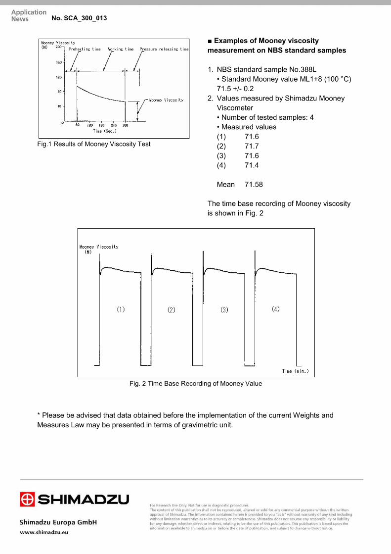
Fig.1 Results of Mooney Viscosity Test
■ Examples of Mooney viscosity measurement on NBS standard samples 1. NBS standard sample No.388L
• Standard Mooney value ML1+8 (100 °C) 71.5 +/- 0.2
2. Values measured by Shimadzu Mooney Viscometer • Number of tested samples: 4 • Measured values (1) 71.6 (2) 71.7 (3) 71.6 (4) 71.4 Mean 71.58
The time base recording of Mooney viscosity is shown in Fig. 2
Fig. 2 Time Base Recording of Mooney Value
* Please be advised that data obtained before the implementation of the current Weights and Measures Law may be presented in terms of gravimetric unit.
No. SCA_300_013

■ Introduction Music cassette tapes are used by an enormous number of music lovers to enjoy beautiful sounds whenever and wherever they wish. High quality audiotapes with low noise levels are required to reproduce the full dynamic range of any music with a stable and balanced sound volume. Ultra micro magnetic particles are scattered on the surface of the high polymer substrates of audiotapes. Audiotapes are classified into several types depending on the kinds of magnetic materials, each of which have respective frequency characteristics. The following presents the result of surface hardness evaluation performed on audiotapes from several manufacturers using the Shimadzu Dynamic Ultra Micro Hardness Tester Model DUH. This unit works on the principle of a micro area measuring technique for providing information about the surface hardness of tape materials.
Measurement of hardness of audiotapes (1) Samples: Brand A TYPE1 (NORMAL) Brand B TYPE1 (NORMAL) Brand C TYPE2 (CrO2) Brand D TYPE2 (CrO2) Brand E TYPE4 (METAL) Brand F TYPE4 (METAL) (2) Testing machine 1) Shimadzu Dynamic Ultra Micro Hardness
Tester Model DUH 2) Thin film attachment (type 2)
Test Mode 2 Cal. Mode 1 (115° triangular
pyramid indenter) Auto or Manual Auto F.S. Depth 2µm Max. Load 0,5gf Loading Speed 5 or 10 After Time 5sec Pre Time 5sec LOT 3
Table 1 Test Conditions
Material Testing System DUH
Evaluation of Surface Hardness of Audiotapes with Shimadzu Dynamic Ultra Micro Hardness Tester Model DUH No. SCA_300_014

No. SCA_300_014
Fig.1 shows dynamic hardness determined by the difference of displacement at two different loads.
Fig. 1 Load – Indentation Depth Curves for Audiotape (Type 1)
Dynamic hardness was calculated by the following equation:
𝐷𝐷𝐷𝐷𝐷𝐷𝐷𝐷(115°) = 37,838 ∙𝑃𝑃𝑃𝑃2
(𝐷𝐷𝐷𝐷2 − 𝐷𝐷𝐷𝐷1)2∙ �1 −�
𝑃𝑃𝑃𝑃1𝑃𝑃𝑃𝑃2�
2
DH(115°): Dynamic Hardness P1: Small testing load (gf) P2: Large testing Load (gf) D1: Indentation depth at P1 (µm) D2: Indentation depth at P2 (µm)
Figs.2, 3 and 4 show hardness variations of respective tapes of types 1, 2, and 4 at various depths. The tape type 2 of brand C showed the highest surface hardness. The tape type 2 from brand D showed a hardness peak at 0.4 to 0.6 μm, suggesting a hard layer at that depth. The metallic tapes of type 4 from brands E and F show similar hardness properties. As seen above, useful information is attainable for evaluating micro hardness differences due to different processing or treatments of tape surfaces.
Fig. 2. Hardness from Surface towards Depth Direction on Audiotape Type 1
Fig. 3 Hardness from Surface towards Depth Direction on Audiotape Type 2
Fig. 4 Hardness from Surface towards Depth
Direction on Audiotape Type 4

The Shimadzu Flowtester Model CFT is used for measurement of melting viscosity and rheological properties of raw materials such as thermo plastics, thermosetting resins, and ceramics, or for determination of temperature and pressure of pressing or injection molding. Two testing modes are available, the constant temperature mode and constant heating rate mode. The former is a method of pressing specimens in a condition of constant temperature, and is suitable for general quality control. The latter is a method pressing specimens in a constant rate heating mode and is often used in measurements of softening and hardening temperatures for flowability evaluation. The following presents the results of flow tests performed in the constant heating rate mode on four kinds of plastics.
■ Softening - flowability curve of polycarbonate resin in constant heating rate mode (Fig.1)
■ Test conditions:
Test temperature:
preset temperature 250 °C to max. 300 °C
Constant heating rate:
6 °C / min
Pressing condition:
Pressure: 10 kgf/cm2
Die: 1 mm D x 10mm (diam. x length)
Material Testing System CFT
Flowtester Flow Tests of Various Kinds of Plastics with Shimadzu Flowtester Model CFT No. SCA_300_017

Fig. 1 Softening – Flowability Curve of Polycarbonate Resin in Constant Heating Rate Mode
■ Softening - flowability curve of polyurethane resin in constant heating rate mode (Fig. 2)
Test temperature:
Preset temperature 100 °C to max. 200 °C
Constant heating rate:
5 °C/min
Pressing conditions:
Pressure: 10 kgf/cm2
Die: D1 x 1 mm(diam. x length)
Fig. 2 Softening- Flowability of Polyurethane Resin in Constant Heating Rate Mode
■ Softening - flowability curve of polyester resin in constant heating rate mode (Fig. 3)
Test temperature:
preset temperature 220 °C to max. 350 °C
Constant heating rate:
3 °C/min
Pressing conditions:
Pressure: 50 kgf/cm2
Die: D 0.5 x 1 mm (diam. x length)
Fig. 3 Softening- Flowability of Polyester Resin in Constant Heating Rate Mode
■ Softening - flowability curve of polychlorinated resin in constant heating rate mode (Fig.4)
Test temperature:
Preset temperature 150 °C to max. 300 °C
Constant heating rate:
6 °C/min
Pressing conditions:
200 kgf/cm2
Die: D1 x 10 mm (diam. x length)
No. SCA_300_017

Fig. 4 Softening- Flowability of Polychlorinated Vinyl in Constant Heating Rate Mode
■ Softening - flowability characteristic curves As temperature is elevated at a given constant rate, the flow rate, apparent viscosity, shear rate, or shearing stress of respective resin specimens can be recorded at any test temperature.
* Please be advised that data obtained before the implementation of the current Weights and Measures Law may be presented in terms of gravimetric unit.
No. SCA_300_017

■ Introduction Light, strong and rust-free plastic tubes (pipes) are widely used for transporting liquids and gases, and for insulating and protecting electrical wiring. In these fields, the hardness of the tube material is an important factor that affects the usage conditions. If the tube is cut lengthways and held flat before measuring its hardness, the elasticity of the plastic causes minute bending (see Fig. 1) that impedes accurate measurement. Here, we present results from a test method that is ideal for such situations. 1. Sample (Plastic Tube) 1) Sample name: Plastic tube 2) Sample No.: No.1 to No.3 3) Sample size: ᴓ2.2 (Outer diameter) x ᴓ1.2
(Internal diameter) x 10 (Length) mm
2. Test conditions 1) Testing machine: Shimadzu Dynamic Ultra
Micro Hardness Tester DUH-W201S 2) Indenter: Triangular pyramid indenter with
tip angle 115° (Berkovitch type) 3) Test mode: Load - Load hold test 4) Test force: 9.8 mN 5) Loading rate: 0.284 mN/sec 6) Sample holding time: 1 sec 7) Temperature: 25 ℃
Material Testing System DUH
Hardness Measurement of Plastic Tubes using the Shimadzu Dynamic Ultra Micro Hardness Tester DUH-W211S
No. SCA_300_021

No. SCA_300_021
1. Test Method The sample (plastic tube) was cut lengthways into two and set on a metal bar (pin gauge ᴓ 1.2) as shown in Fig.2 to measure its hardness by indentation.
2. Test Results 1) Results of the hardness measurements are shown in Table 1, Fig.3 and Fig.4. 2) The DHT115 values in Table 1 shows that the Sample No.1 is the hardest, followed by No.2 and No.3 in that order, when tested with the test force of 9.8 mN. Fig.4 (graph that presents the relation of test force and indentation depth) shows that the elasticity of the tube is correctly detected, validating the effectiveness of the data.
Table 1 Hardness measurement results (mean values)
Sample name Sample No. Dynamic hardness (DHT115) Test force
(mN) Indentation depth
(µm) Tube A No. 1 15.6 9.8 1.55 Tube B No. 2 13.7 9.8 1.66 Tube C No. 3 11.7 9.8 1.8
Ref.) Dynamic hardness was calculated as follows: DHT11S=3,8584 P/ D2
DHT115:Dynamic hardness (115° triangular indenter) P: Test force (mN) D: Indentation Depth (µm)
0
5
10
15
20
No. 1 No. 2 No. 3
Fig. 3 Sample number and dynamic hardness (DHV)
Fig. 4 Test force – indentation depth curve
* Please be advised that data obtained before the implementation of the current Weights and Measures Law may be presented in terms of gravimetric unit.
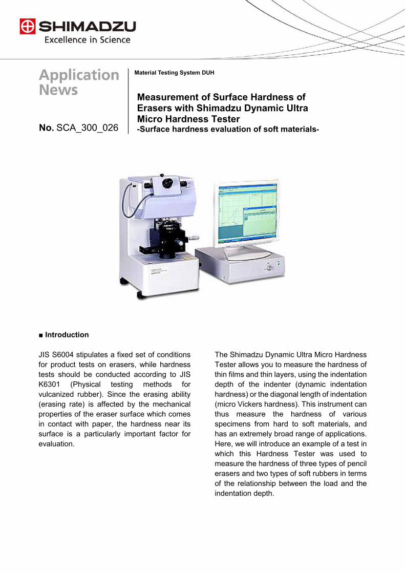
No.????
■ Introduction JIS S6004 stipulates a fixed set of conditions for product tests on erasers, while hardness tests should be conducted according to JIS K6301 (Physical testing methods for vulcanized rubber). Since the erasing ability (erasing rate) is affected by the mechanical properties of the eraser surface which comes in contact with paper, the hardness near its surface is a particularly important factor for evaluation.
The Shimadzu Dynamic Ultra Micro Hardness Tester allows you to measure the hardness of thin films and thin layers, using the indentation depth of the indenter (dynamic indentation hardness) or the diagonal length of indentation (micro Vickers hardness). This instrument can thus measure the hardness of various specimens from hard to soft materials, and has an extremely broad range of applications. Here, we will introduce an example of a test in which this Hardness Tester was used to measure the hardness of three types of pencil erasers and two types of soft rubbers in terms of the relationship between the load and the indentation depth.
Material Testing System DUH
Measurement of Surface Hardness of Erasers with Shimadzu Dynamic Ultra Micro Hardness Tester -Surface hardness evaluation of soft materials-
No. SCA_300_026

No. SCA_300_026
Test results
Eraser (A) No. Load (gf) Depth (µm) Hardness No. Load (gf) Depth (µm) Hardness
1 0.114 21.85 0.0090 2 0.114 21.53 0.0093 3 0.098 19.94 0.0094
Average 0.109 21.11 0.0092
Eraser (B) No. Load (gf) Depth (µm) Hardness No. Load (gf) Depth (µm) Hardness
1 0.127 15.17 0.0209 2 0.115 14.50 0.0207 3 0.114 13.44 0.0238
Average 0.118 14.37 0.0218
Eraser (C) No. Load (gf) Depth (µm) Hardness No. Load (gf) Depth (µm) Hardness
1 0.179 13.28 0.0384 2 0.147 12.33 0.0366 3 0.159 13.71 0.0320
Average 0.162 13.11 0.0357
Soft rubber (A) No. Load (gf) Depth (µm) Hardness No. Load (gf) Depth (µm) Hardness
1 0.029 17.71 0.0035 2 0.033 19.21 0.0034 3 0.028 17.27 0.0036
Average 0.030 18.06 0.0035
Soft rubber (B) No. Load (gf) Depth (µm) Hardness No. Load (gf) Depth (µm) Hardness
1 0.312 17.82 0.0372 2 0.342 18.86 0.0364 3 0.370 19.47 0.0369
Average 0.342 18.72 0.0369
Fig. 1 Eraser (A)
Fig. 2 Eraser (B)

No. SCA_300_026
Fig. 3 Eraser (C)
Fig. 4 Soft Rubber (A)
Fig. 5 Soft Rubber (B)
Figs. 1, 2 and 3 are diagrams of the test results that indicate the load-indentation depth relationships for pencil erasers (A), (B), and (C) respectively. Figs. 4 and 5 display those for soft rubbers (A) and (B). In each respective diagram, the data obtained from three tests and their average values are indicated as four curves. The average value is shown in the first curve in each diagram. For the hardness (DH) measurement, a triangular pyramid indenter with a tip angle of 115 degrees was used, and the calculation was performed using the following equation: DH= 37,838 P/h2 P: Test Load (gf) h: Indentation depth (µm)

■ Introduction Some of today's synthetic rubbers feature unique properties such as minimal elasticity or a thermoplastic nature that needs no vulcanization, which make them particularly appropriate for some applications. Such new features and functions of synthetic rubbers are blurring the line between rubbers and plastics. Many kinds of rubbers are appearing on the market due to the development of new rubber materials, fillers, vulcanizing agents, plasticizers etc. The viscosity test of rubber materials is one important method for evaluating various functions for rubber. The Shimadzu Automatic Mooney Viscometer is an excellent machine for the efficient performance of Mooney viscosity and Mooney scorch tests.
■Test results of Mooney viscosity and scorch (1) Butyl type rubber (Fig.1)
Fig. 1 Butyl Type Rubber
Material Testing System SMV
Measuring and Controlling Performance of Shimadzu Mooney Viscometer Model SMV in Viscosity Tests on Rubber Materials
No. SCA_300_028

(2) Natural rubber (Fig. 2)
Fig. 2 Natural Rubber
(3) Nitrile rubber (Fig. 3)
Fig. 3 Nitrile Rubber
* Please be advised that data obtained before the implementation of the current Weights and Measures Law may be presented in terms of gravimetric unit.
No. SCA_300_028

Epoxy resin, characterized by its excellent electrical, mechanical and adhesive properties as well as its chemical proof properties, is utilized in a wide range of materials including electric insulators, paints, structural assemblies, adhesive agents, etc. The thermosetting nature of epoxy resin materials, processed in combination with curing agent, has to be evaluated in terms of curing speed by the extruding type flow test method, and not by usual physical strength methods. The Shimadzu Flow Tester Model CFT, with the ability to test flow rates under pressures and shear rates similar to those of the usual forming process, can be used not only for testing thermoplastic resin, but also thermosetting resin, adhesive agents, copying toner, rubber materials, ceramic materials, foods, cosmetics, medicines, etc. The following presents the results of measurement in curing time of epoxy resin performed with the Shimadzu Flow tester Model CFT.
■ Outline of Shimadzu flow tester CFT 1) Method of pressure application: Constant
load extruding 2) Extruding pressure: Max. 500 kgf/cm2 3) Testing mode: Constant temperature or
constant heating rate 4) Test temperature: Max. 400 °C 5) Cylinder diameter: 11.329 mm (1 cm2
cross sectional area) ■ Testing conditions Specimen: Epoxy resins Couring agent: Anhydrous phtalic acid + acid absorption amine Temperature conditions: Constant temperature mode, 150 °C. Extruding condition: Pressure kgf/cm2 Die irifice: Diam 1.0 x Length 1.0 mm ■ Test results Figs.1, 2 and 3 show flow curves of three different epoxy resins with different concentrations of curing agent. Flow starting times, curing times etc. for respective specimens can be discerned immediately from these curves. Test conditions and data such as shear stress, flow rate, shear rate, viscosity, etc. are simultaneously printed automatically at the portion above the graph, presenting all necessary information on a sheet. The three curves of Figs.1, 2 and 3 are shown in Fig. 4 in overlap mode for at-a-glance comparison with each other. Overlap mode helps present mean values and deviation of test data for a single specimen as well.
Material Testing System CFT
Test on Thermosetting Resin with Shimadzu Flow Tester Model CFT No. SCA_300_031

Figure 1: Flow curve of epoxy resin (A)
Figure 2: Flow curve of epoxy resin (B)
No. SCA_300_031
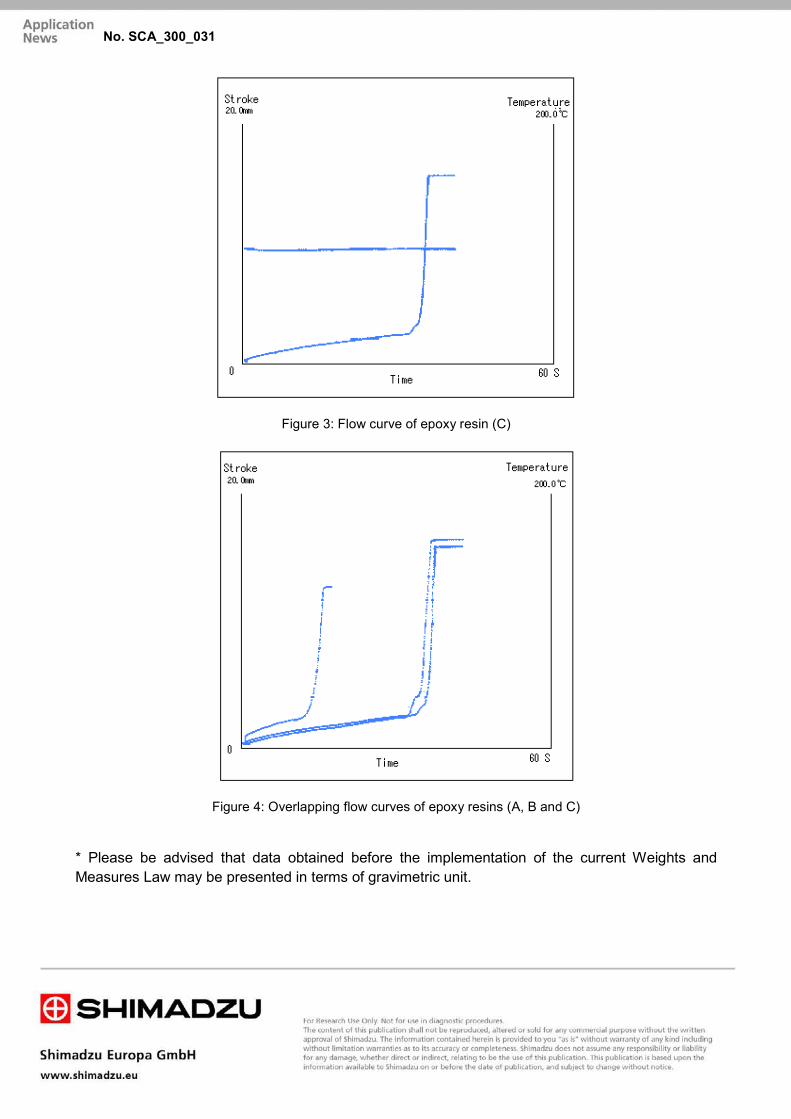
Figure 3: Flow curve of epoxy resin (C)
Figure 4: Overlapping flow curves of epoxy resins (A, B and C)
* Please be advised that data obtained before the implementation of the current Weights and Measures Law may be presented in terms of gravimetric unit.
No. SCA_300_031

ApplicationNews
No.i253
Material Testing System
Tensile Test of Plastic Materials
LAAN-A-AG-E017
Introduction
The physical characteristics of plastic materials are an essential part of product design and quality control. Various materials tests are performed because of this, of which the most basic test is tensile testing that is cited in many product specifications. The tensile properties of plastic materials assessed by tensile testing include strength, elastic modulus, and breaking strain. Tensile testing of plastics was once performed according to the standard test methods described in ISO 527-1 (JIS K 7161), but ISO 527-1 was revised substantially in 2012 (and JIS K 7161 in 2014). This revision resulted in a number of important changes, of which the main changes are summarized below.First, the preferred gauge length for type 1A geometry specimens was changed to 75 mm. The previous gauge length of 50 mm is still allowed, but since it became possible to set a longer gauge length, a gauge length of 75 mm is preferred since using this length makes it easier to produce a break within the gauge length. Also, a gauge length of 75 mm is recommended due to the relationship between gauge length and extensometer accuracy that is mentioned below. ISO 527-1 (JIS K 7161) noted that tests must be performed within a standard error of 1 % to calculate elastic modulus accurately. Fig. 1 shows absolute values for the extensometer accuracy required when using a 75 mm and 50 mm gauge length. It shows the absolute accuracy of a 75 mm gauge length is ±1.5 μm, while the absolute accuracy of a 50 mm gauge length is ±1.0 μm. In other words, performing the same test with a 75 mm gauge length increases the permissible range of absolute accuracy. This widens the choice of extensometers and allows the TRViewX non-contact digital video extensometer (absolute accuracy of ±1.5 μm) to be used for standard testing.The revision also added a method for calculating strain at yield point. The previous Method A calculated strain with equation (1). The newly added Method B calculates strain with equation (2).
εt
ΔLt
εy
Lt
L
: Nominal strain: Initial distance between grips [mm]
: Increase in distance between grips [mm]
: Yield strain: Increase in distance between grips beyond theyield point [mm]
εt = (1)
(2)
Lt
L
εt =εy +ΔLt
L
Method B is preferred for materials that exhibit yielding and necking. Fig. 2 shows an illustrated image of a st ra in ca lculat ion performed us ing Method B. Shimadzu's TRAPEZIUM X software supports both Method A and Method B.In this article, PP (polypropylene), PVC (polyvinyl chloride) and PC (polycarbonate) specimens are tested in accordance with current standards.
Test data
Elastic modulus
Str
ess
(σ
)
Strain (ε)
ε1 : 0.05 % ε2 : 0.25 %
Displacement
0.0375 mm 0.1875 mm
(150±1.5) μm
(100±1.0) μm
Displacement
0.025 mm 0.125 mm
GL75
GL50
Fig. 1 Comparison of Absolute Accuracy between 75 mm
and 50 mm Gauge Lengths
Strain (ε)
Stre
ss (σ
)
εy
ΔLt
L
Fig. 2 Strain Calculated by Method B

SpecimenStrength
[MPa]
Elastic Modulus
[GPa]
PP 32.5 1.66
PC 63.3 2.30
PVC 73.4 3.23
SpecimenStrength
[MPa]
Elastic Modulus
[GPa]
PP 32.5 1.63
PC 63.7 2.26
PVC 73.4 3.12
ApplicationNews
No.
© Shimadzu Corporation, 2016
For Research Use Only. Not for use in diagnostic procedure.
This publication may contain references to products that are not available in your country. Please contact us to check the availability of these
products in your country.
The content of this publication shall not be reproduced, altered or sold for any commercial purpose without the written approval of Shimadzu.
Company names, product/service names and logos used in this publication are trademarks and trade names of Shimadzu Corporation or its
affiliates, whether or not they are used with trademark symbol “TM” or “®”. Third-party trademarks and trade names may be used in this
publication to refer to either the entities or their products/services. Shimadzu disclaims any proprietary interest in trademarks and trade names
other than its own.
The information contained herein is provided to you "as is" without warranty of any kind including without limitation warranties as to its
accuracy or completeness. Shimadzu does not assume any responsibility or liability for any damage, whether direct or indirect, relating to the
use of this publication. This publication is based upon the information available to Shimadzu on or before the date of publication, and subject
to change without notice.
www.shimadzu.com/an/
i253
First Edition: Aug. 2016
Measurement System
Measurements were made using an AGS-X table-top precision universal testing instrument, a contact extensometer, and a non-contact digita l v ideo extensometer. A gauge length of 75 mm was used with both extensometers. Table 1 shows a l ist of the equipment used.
Testing Machine : AGS-XLoad Cell : 5 kNGripping Device : Pneumatic parallel gripping deviceGripping Teeth : Single-cut file teethSoftware : TRAPEZIUM X (Single)Displacement Gauge : SG75-10, TRViewX 240S
Table 1 Experimental Equipment
Measured Results
An initial test speed of 1 mm/min was switched to 50 mm/min at 1 mm displacement. The contact extensometer was removed at 1 mm displacement. Fig. 3 shows testing with the SG75-10 and Fig. 4 shows testing with the TRViewX. The respective test results are shown in Table 2 and Table 3, and the stress-strain curve obtained using the SG75-10 is shown in Fig. 5. The results shown in Table 2 and Ta b l e 3 c o n f i r m t h a t t e s t s w e re p e r f o r m e d successful ly since there is almost no difference between them.
Fig. 3 Testing with SG75-10
Fig. 4 Testing with TRViewX
0
10
20
30
40
50
60
70
80
90
100
010 20 30 40 50 60 70 80 90 100 110 120
Displacement (Strain) (%)
Stress (N/mm2 )
PP_1PC_1PVC_1
Fig. 5 Test Results Using SG75-10
Table 2 Test Results Using SG75-10
Table 3 Test Results Using TRViewX
Conclusion
The testing standard for tensile testing of plastic materials has undergone an important revision. Introduct ion of a 75 mm gauge length br ings benef i t s tha t inc lude an inc reased cho ice o f extensometers for elastic modulus measurement and an easier break within the gauge length. Introducing Method B for calculat ing stra in a l lows a more accurate determination of strain, in materials that exhibit yielding and necking in particular. Testing according to the current ISO 527-1: 2012 (JIS K 7 1 6 1 - 1 : 2 0 1 4 ) s t a n d a rd c a n b e p e r f o r m e d successfully using the equipment described in this article.

ApplicationNews
No.i249
Material Testing System
Three-Point Bending Flexural Test of Plastics
(ISO 178, JIS K 7171)
LAAN-A-AG-E014
Introduction
Based on their thermal properties and light weight, plastics have recently come to be used in a variety of applications and sectors, from small gears to airplane fuselages. A variety of tests must be performed to evaluate these materials, from tensile tests to flexural tests and compression tests. Of these, a flexural test is performed to examine material characteristics when flexed by an external force. Because components subject to an external force will flex in reaction to a bending moment, the flexural test is one of the most basic tests used to evaluate materials.Previous testing standards described a three-point bending flexural test for plastics did not require the deflection-measuring system. As a result, tests detected specimen, instrument def lect ion and indenter depression together as a total, which is a method not suited to accurate measurements of flexural modulus of elasticity. New standards (ISO178:2010, Amd.1:2013 and JIS K 7171:2016) have been revised and include either use of a deflection-measuring system with "ISO 9513 Class 1" absolute accuracy of within 1 %, or use of compliance correction to remove testing machine deflection. A three-point bending flexural test was performed on PC, PVC, and GFRP specimens in compliance with the new standards, where the flexural modulus of elasticity of each plastic was calculated using compliance correction and the deflection-measuring instrument.
Measurement System
Measurements were performed using an AGS-X Table-Top Type Universal Test ing Instrument and the deflection-measuring system with a measurement accuracy of within 3.4 μm. The requirements of the new standards when mean specimen thickness is 4 mm are shown in Fig. 1. The value relevant to flexural modulus calculation is 341 μm, where a deflection measuring instrument with absolute accuracy of 1 % of this value (3.4 μm) is required (Fig. 1 shows the flexural modulus of elasticity calculated based on the slope at two points, though the flexural modulus of elasticity could also be calculated based on the linear regression of the curve).Table 1, 2 and 3 show details of the instruments, specimens, and test conditions used. Fig. 2 shows the test apparatus layout. The new standards describe a method A that uses a constant test speed, and a method B that increases the test speed after flexural modulus measurement. Test method A was used with GFRP that has a small maximum flexural strain, and test method B was used with PC and PVC that have a large max imum f lexura l s t ra in , and the tes t speed changeover point was set at 0.3 % flexural strain. Furthermore, since the proportion of external force accounted for by shearing force increases when the span between supports is small1), standards recommend the span between specimen supports is 16±1 times the mean specimen thickness.
Flexu
ral st
ress
σFlexural strain ε
ε1: 0.05 % ε2: 0.25 %
Flexural modulus of elasticity (MPa) = (σ1 - σ2) / (ε2 - ε1)
: 0.05 %
85 μm 426 μm
341±3.4 μm
Thickness of 4 mm
Delection-measuring system with absolute accuracy of 3.4 μm required
: 0.25 %
426 μm
σ2
σ1Test data
Modulus of elasticity
Fig. 1 New Standard Requirements
Testing Machine : AGS-XLoad cell : 1 kNDeflection-measuring system : Deflection measuring device Bending jigs : Loading edge R5, supports R5
Table 1 Equipment Details
Dimensions : 80 mm × 10 mm × 4 mmType : PC, PVC, GFRP (short fiber)
Table 2 Specimen Information
Test speed : 2 mm/minTest speed after measurement of flexural modulus of elasticity
: 100 mm/min (method B)
Span between specimen supports : 64 mm
Table 3 Test Conditions
Fig. 2 Attachment of deflection-measuring system
to Testing Machine

Flexural strength
[MPa]
Flexural modulus
of elasticity [GPa]
PC 104.4 2.44
PVC 123.0 3.48
GFRP 179.4 12.1
Flexural Modulus
of Elasticity [GPa]
Deflection-Measuring
System
Flexural Modulus
of Elasticity [GPa]
Compliance Correction
Difference
(%)
PC 2.44 2.42 1.1
PVC 3.48 3.41 2.1
GFRP 12.1 11.7 3.3
ApplicationNews
No.
© Shimadzu Corporation, 2016
For Research Use Only. Not for use in diagnostic procedure.
This publication may contain references to products that are not available in your country. Please contact us to check the availability of these
products in your country.
The content of this publication shall not be reproduced, altered or sold for any commercial purpose without the written approval of Shimadzu.
Company names, product/service names and logos used in this publication are trademarks and trade names of Shimadzu Corporation or its
affiliates, whether or not they are used with trademark symbol “TM” or “®”. Third-party trademarks and trade names may be used in this
publication to refer to either the entities or their products/services. Shimadzu disclaims any proprietary interest in trademarks and trade names
other than its own.
The information contained herein is provided to you "as is" without warranty of any kind including without limitation warranties as to its
accuracy or completeness. Shimadzu does not assume any responsibility or liability for any damage, whether direct or indirect, relating to the
use of this publication. This publication is based upon the information available to Shimadzu on or before the date of publication, and subject
to change without notice.
www.shimadzu.com/an/
i249
First Edition: Dec. 2016
Test Results
Fig. 3 shows a flexural stress/flexural strain curves. Flexural strain on the horizontal axis was calculated based on results measured using the deflection-measuring system. The curve shows a sudden decrease in flexural stress with GFRP, but no sudden decrease in flexural stress with PC and PVC as these specimens did not break suddenly. Table 4 shows the results obtained for flexural strength and flexural modulus of elasticity for each material.Table 5 shows the difference in flexural modulus when calculated based on the deflection-measuring system and compliance correction. The results show a difference of around 1 to 2 % for plastics like PC and PVC with a flexural modulus of elasticity of 2 to 3 GPa, and a difference of around 3 % for specimens like GFRP with a high flexural modulus of elasticity.
0
40
80
120
160
200
0 2 4 6 8 10 12
Flexu
ral st
ress
(M
Pa)
Flexural strain (%)
PC
PVC
GFRP
Fig. 3 Test Results
Table 4 Test Results
Table 5 Difference in Flexural Modulus of Elasticity Results
Using Compliance Correction and Deflection-Measuring
System
Deflection according to compliance correction and the deflection-measuring system is compared in Fig. 4, which shows deflection obtained by each method during the initial period of the test of GFRP. Results obtained from the deflection-measuring system are represented by the solid line, and results obtained by compliance correction are represented by the dotted line. The graph shows the difference between the lines.
0
10
20
30
40
0 0.05 0.1 0.15 0.2 0.25 0.3
Flexu
ral st
ress
(M
Pa)
Flexural strain (%)
GFRP (Delection-measuring system)
GFRP (Compliance Correction)
Fig. 4 Flexural Stress/Flexural Strain Curve of GFRP
(Flexural strain 0 % to 0.3 %)
Conclusion
Plastics were subjected to a three-point bending flexural test with a method compliant with new standards (ISO178:2010, Amd.1:2013 and JIS K 7171:2016). Results showed the higher the flexural modulus of elasticity of a material, the larger the difference between the flexural modulus of elasticity calculated using a deflection-measuring system and compliance correction. Exact measurement of displacement with a deflection-measuring system is required for a proper evaluation of materials in compliance with the new standards.The equipment setup employed in this article can be used to perform three-point bending flexural tests of plastics in compliance with the new standards.
Reference1) Takeshi Murakami, Shimadzu Review Vol. 71, Issue 3/4 (2014)

The Autograph Series features the ability to freely change test conditions while testing in addition to the reciprocating function (tension - compression). Shown below is an example of a tension - compression major deformation test. This test is popular for evaluating the dynamic characteristics of rubber vibration isolators, executed by the Autograph. Measurement was taken to record changes in energy loss (absorbed energy) on a hysteresis loop. Load and deformation were applied to an anti-vibration rubber developed for use in the architecture and civil engineering fields, load and deformation were then increased at return point per cycle... ■ Test conditions 1) Cycle test by means of load control
Test Mode Cycle Tens/Comp. (Tens.)
Minimum Load -50 kgf
Maximum Load 50 kgf
Test Speed 2 mm/min
Load Cell 10000 kgf
F/S Load 500 kgf
The above were load conditions at first cycle (+/- 50 kgf).+/- 100 kgf, +/- 200 kgf, +/- 300 kgf and +/-400 kgf were applied successively thereafter
Test Mode Cycle Tens/Comp. (Tens.)
Minimum Stroke -1 mm
Maximum Stroke 1 mm
Test Speed 2 mm/min
Load Cell 10000 kgf
F/S Load 500 kgf
The above were displacement conditions at first cycle (+/- 1 mm). +/- 2 mm, +/- 3 mm, +/- 4 mm and +/- 5 mm were applied successively thereafter.
Material Testing System AGS-X
Tension - Compression Major Deformation Test of Rubber Vibration Isolator by Shimadzu Autograph Series
No. SCA_300_038
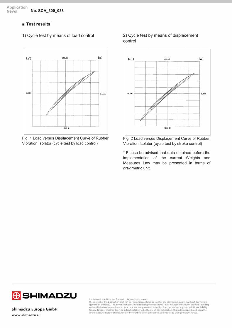
■ Test results 1) Cycle test by means of load control
Fig. 1 Load versus Displacement Curve of Rubber Vibration Isolator (cycle test by load control)
2) Cycle test by means of displacement control
Fig. 2 Load versus Displacement Curve of Rubber Vibration Isolator (cycle test by stroke control)
* Please be advised that data obtained before the implementation of the current Weights and Measures Law may be presented in terms of gravimetric unit.
No. SCA_300_038

Plastics often show viscoelasticity. They can be deformed by a relatively small external force, but return to their original state if the external force is removed. In addition, many plastics have a hardness dependent on their mechanical properties. Elastic recovery and temperature are the essential factors for the evaluation of the mechanical hardness of plastics. The Shimadzu Dynamic Ultra Micro Hardness Tester allows you to measure the hardness of thin films and thin layers using the indentation depth of the indenter (dynamic indentation
hardness) or the diagonal length of indentation (micro Vickers hardness). This instrument can thus measure the hardness of various specimens from hard to soft materials, and has an extremely broad range of applications. Here, we will introduce an example of a hardness test in which this Ultra Micro Hardness Tester, installed in a room of constant temperature, was used to measure and compare the elastic recovery of two types of plastics, which have similar dynamic indentation hardness: nylon 66 and polyethylene.
Test conditions Indenter: Vickers Maximum load: 50 gf Retention time: 1 sec Deformation scale: 10 µm
Material Testing System DUH
Evaluation of Elastic Recovery in Hardness Measurement of Plastic Materials with Shimadzu Dynamic Ultra Micro Hardness Tester No. SCA_300_039

Test method Load is applied up to 50 gf using the cyclic loading function of the Ultra Micro Hardness Tester. After the load is retained for one second, the load begins to decrease until it reaches zero. The depth of the indenter is measured at two points, when the load reaches
50 gf and when it returns to zero. The discrepancy in load between these two points is regarded as the amount of elastic recovery. The dynamic indentation hardness when the Vickers indenter is used is calculated by the following equation:
DH = 37,838 P/h2
P : Test load (gf) H : Indentation depth (µm)
Table 1 Test Results
Nylon 66 Polyethylene Load (gf) 50,00 50,00 Indentation depth when load reaches 50gf (µm) 18,20 19,13 Indentation depth when load returns to 0 (µm) 7,65 13,06 Amount of elastic recovery (µm) 10,55 6,07 Dynamic indentation hardness 5,71 5,17
Test results The test results are shown in Table 1, Figure 1 and 2. As indicated by the table and figures, there is a major difference in the amount of elastic recovery between these two types of plastics despite their similar dynamic indentation hardness (that of nylon 66 is slightly greater
than that of the other). It is therefore presumed that in the method to measure the diagonal length of indentation, nylon 66 will exhibit a considerably higher hardness than that of polyethylene.
Fig. 1 Diagram of load Indentation Depth Relationship for Nylon 66
No. SCA_300_039

Fig. 2 Diagram of load Indentation depth for Polyethylene
* Please be advised that data obtained before the implementation of the current Weights and Measures Law may be presented in terms of gravimetric unit.
No. SCA_300_039

■ Introduction Rubber products are produced by forming rubber compounds (mixtures of rubber and additives that provide specific functional characteristics) in a mold and then applying heat to provide an elastic body. Therefore, the fluidity of rubber compounds can have a major effect on molding quality. Unformed rubber compounds change their characteristics after long storage periods, which can cause fluidity to deteriorate or the molding process to fail, depending on how they are stored. Here, the example, which evaluated the fluidity change by the storage method of the unvulcanized rubber, is introduced.
■ Fluidity Change by the Storage Method of Unvulcanized Rubber
In this case, a rubber compound was stored at ambient temperature and low temperature for 14 days and 28 days immediately after kneading and then the fluidity was evaluated. The results showed that the given sample could be stored at low temperatures without a significant change in fluidity, even after one month. Using the CFT-EX series allows evaluating the rubber compounds storage temperatures and storage periods without actually having to mold any parts.
Test Method Constant temperature test
Die Diameter 0,5 mm
Die Length 1 mm
Test Temperature 280 ℃
Test Pressure 20,1 MPa
Preheating Time 0 sec
Sample Size 1.6 g Test Conditions
Material Testing System CFT
Fluidity Evaluation of Unvulcanized Rubber No. SCA_300_043

Storage Temperature
Storage Temperature Viscosity(Pa•s)
Ambient Temperature
0 395,7 14 568,1 28 600,0
Low Temperature
0 395,7 14 447,5 28 419,3
Test Result
■ CFT-EX can use evaluation of unvulcanized rubber CFT-EX, which can evaluate thermosetting and thermoplastic resin in evaluation of unvulcanized rubber, is recommended. The feature of CFT-EX
• Higher Level Evaluation Using a Variety of Analysis Methods The evaluation of thermosetting resin and constant heating rate test is possible.
• Smooth, Easy Test Flow New software compatible with Win7,8.1
• Supported by More Than 50 Years of Technology and Know-How Abundant applications cultivated for years
Changes in Viscosity Due to Storage Methods
No. SCA_300_043

When thermosetting resins are heated, they melt and are able to flow, but further increases causes curing. The minimum viscosity value, the time it takes to reach that minimum, curing depend on the temperature used to melt the resin. Unless these viscosity and time molding process, they can result in molding defects. For resins, characteristic values due to other factors. Therefore, controlling the resin viscosity is very important to ensure vary and good products are produced.
■ Measurement of the Minimum Melt Viscosity Value The fluidity properties of thermosetting resins are often measured using constant temperature testing. Unlike thermoplastic resins, the thermoset viscosity is constantly changing. Therefore, the minimum melt viscosity value can be determined automatically by using automatic constant temperature testing. In this case, three types of thermosetting resins were tested using the constant temperature method. The testing pressure was selected so that the sample would melt and flow and then stop flowing due to curing. Test condition Viscosity-Temperature Graph The viscosity-time graph, which shows the change in viscosity over time, indicates that the sample melts and starts to flow after about 3 seconds, reaches its minimum viscosity after about 10 seconds, and then stops flowing after about 18 seconds. The CFT calculates viscosity by measuring the amount of piston movement (movement speed) during constant test force extrusion.
Therefore, even when the sample cures due to heating, the piston displacement merely stops, which has no effect on controlling test force. Consequently, it provides extremely stable and highly reproducible test.
Viscosity-Temperature Graph
Material Testing System CFT
Viscosity Evaluation of Thermoplastic Resins (Epoxies)
No. SCA_300_054
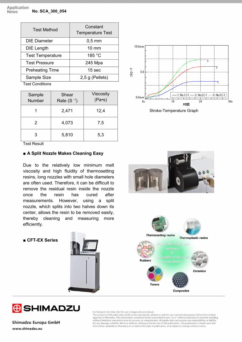
Test Method Constant Temperature Test
DIE Diameter 0,5 mm DIE Length 10 mm Test Temperature 185 °C Test Pressure 245 Mpa Preheating Time 15 sec Sample Size 2,5 g (Pellets)
Test Conditions
Sample Number
Shear Rate (S -1)
Viscosity (Pa•s)
1 2,471 12,4
2 4,073 7,5
3 5,810 5,3
Test Result
Stroke-Temperature Graph
■ A Split Nozzle Makes Cleaning Easy Due to the relatively low minimum melt viscosity and high fluidity of thermosetting resins, long nozzles with small hole diameters are often used. Therefore, it can be difficult to remove the residual resin inside the nozzle once the resin has cured after measurements. However, using a split nozzle, which splits into two halves down its center, allows the resin to be removed easily, thereby cleaning and measuring more efficiently.
■ CFT-EX Series
No. SCA_300_054

Increasingly high performance engineering resins are being developed for use in a wide range of fields, such as the automotive industry, consumer electronics, office automation equipment, for their various functional characteristics. Some of the criteria that have become especially important for evaluating the performance of such materials is impact resistance and its associated material properties, such as strength and rigidity. In addition to evaluating materials in terms of conventional static tensile strength, high-rate tensile strength, longitudinal elasticity, and strain measurements up to the breakpoint are expected to become important new parameters for materials development. This example describes testing the high- rate tensile strength of a flat plate specimen of ABS resin and measuring strain up to the breakpoint. Images of the high-rate tensile test were captured with a high-speed video camera and image analysis software was used to measure the strain between gauge length on the specimen. ■ Tensile test specimen Fig. 1 shows the dumbbell-shaped flat ABS resin tensile test specimen mounted in the grips of the high- rate tensile testing machine. A chuck extensometer, capable of measuring the relative displacement of the fixed end and the upper grip, is attached to the top right of the specimen. A matrix of black dots is printed on the surface of the specimen. The strain between gauge length can be measured by using a high-speed video camera to record a moving image of the tensile test and automatically tracking the movement of the specified dots.
(1) Specimen Material: ABS resin (2) Specimen Dimensions: 110 (L) × 10 (W)
× 3 (T) mm and 19 mm wide grip tab (3) Dot Specifications: 0.5 mm diameter,
spaced 2 mm apart
Figure 1: Tensile test specimen mounted in grips
■ Measuring High-Rate Tensile Strength and Recording Video Image Tensile test was performed using the HITS-T10 hydroshoot hydraulic tensile machine. The HPV-2A high speed camera was mounted in front of the testing machine to capture 100 video frames of the specimen of the specimen behavior during tensile testing. Conditions for tensile testing and recording video in this example are indicated below: (1) Tensile rate: 3 m/s (2) Grip distance: 75 mm (3) Gauge length measuring strain: 30 mm (4) Test force measurement: 10 KN load cell (5) Data collection: 250 KHz (6) Recording speed: 32 kfps (7) Light source metal halide light
Material Testing System HITS
Breaking strain measurement of ABS resin No. SCA_300_057
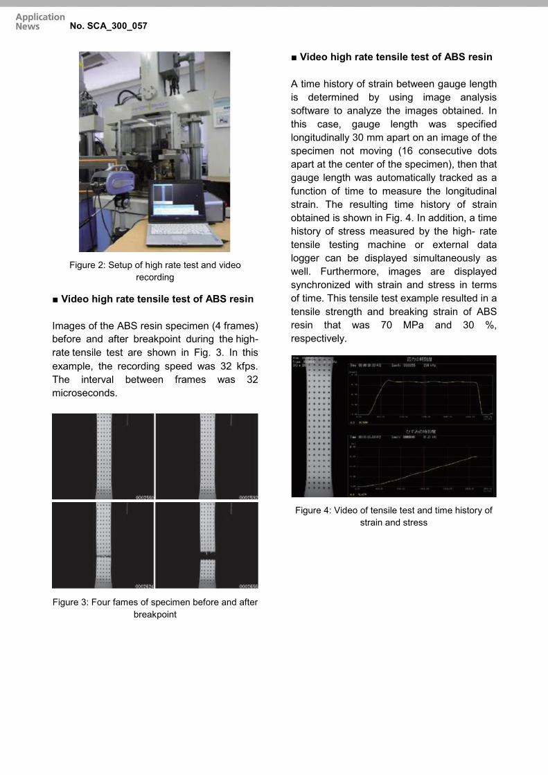
Figure 2: Setup of high rate test and video recording
■ Video high rate tensile test of ABS resin Images of the ABS resin specimen (4 frames) before and after breakpoint during the high-rate tensile test are shown in Fig. 3. In this example, the recording speed was 32 kfps. The interval between frames was 32 microseconds.
Figure 3: Four fames of specimen before and after
breakpoint
■ Video high rate tensile test of ABS resin A time history of strain between gauge length is determined by using image analysis software to analyze the images obtained. In this case, gauge length was specified longitudinally 30 mm apart on an image of the specimen not moving (16 consecutive dots apart at the center of the specimen), then that gauge length was automatically tracked as a function of time to measure the longitudinal strain. The resulting time history of strain obtained is shown in Fig. 4. In addition, a time history of stress measured by the high- rate tensile testing machine or external data logger can be displayed simultaneously as well. Furthermore, images are displayed synchronized with strain and stress in terms of time. This tensile test example resulted in a tensile strength and breaking strain of ABS resin that was 70 MPa and 30 %, respectively.
Figure 4: Video of tensile test and time history of strain and stress
No. SCA_300_057

■ Video high rate tensile test of ABS resin
Producing a stress-strain curve, which is easy for static tensile testing, is an extremely difficult technical challenge for high-rate tensile testing. Strain gauges can only measure a small range and contact type extensometers do not work for shock. In this example, a stress-strain curve was obtained for ABS resin by synchronizing the video image timing with the test force.
A stress-strain curve up to the specimen breakpoint is shown in Fig. 5.
In this way, combining a high-rate tensile testing machine, high-rate video camera, and image analysis software, enables simultaneously evaluating high-rate tensile properties, including breaking strain, and visualizing changes in the status of resins.
Figure 5: Stress-strain curve up to breakpoint
No. SCA_300_057

9. Others

9. Others
UNIVERSAL, HARDNESS AND VISCOSITY AND FLOW TESTING
This chapter covers applications outside routine materials test-ing. They show that machine testing capabilities can also meet creativity of the laboratory staff.
To categorize the applications, they are allocated to the mate-rial testing machines. In total, 15 versatile and exciting appli-cations are described on the following pages.
Micro Vickers Hardness TesterDeveloped particularly for less experienced operators, the Micro Vickers Hardness testers feature automatic length mea-surement. The HMV-G series is capable of automatic recogni-tion of total sample image and edges through easy-to-use software. Even complicated shapes can be recognized.
DUH Ultra Micro Hardness Tester Shimadzu`s DUH tester is useful in a wide range of applica-tions for evaluating the surface hardness of solid samples based on the relation between indenting load and indentation depth. The DUH series has been designed for testing of materi-als in the micro field that cannot be handled by regular tes-ters. The DUH series focusses surface strength evaluations on every type of material, e.g. extra fine wire, pencil leads, pearl surface and hydrogen storage alloy as used in fuel cell batteries.
Autograph AGS-X universal material testing system Providing high-level control and intuitive operation, the Autograph AGS-X series sets a new standard for strength eval-uations. The series offers superior performance and practical testing solutions for a wide array of applications such as paper friction test, spring compression test and measurement of strength of glass.
EZ-X universal material testing system The compact-sized EZ-X series provides accurate results due to a high-precision load cell. It supports a huge number of appli-cations, e.g. medical, plastics, electronics, film/textile and food. In addition to the applications mentioned in this book, please see the Big Breakfast Test.
Material Testing System CFTThe CFT-EX series is ideal for research and development, pro-duction process and quality control. The system evaluates flu-idity and thermal properties of various materials such as ther-moplastic and thermosetting resins, toners, composites, rubbers and other flowable materials.

9. Others
No.i248 Mechanical strength evaluation of functional film used in smartphones
No.10 Measurment for monotonic equibiaxial flexural strength of glass ASTM C1499 01
SCA_300_007 Compression test of a liquid crystal spacer (columnar) under different temperatures
SCA_300_008 Compression tests of liquid crystal spacer using the Shimadzu dynamic ultra micro hardness tester DUH
SCA_300_009 DUH hardness test on extra fine wires
SCA_300_018 Hardness evaluation of pencil leads with Shimadzu dynamic ultra micro hardness tester-bmu
SCA_300_020 Hardness measurement of hydrogen stor-age alloy using the Shimadzu dynamic ultra micro hardness tester DUH
SCA_300_022 Hardness test of ion implanted specimens and valuable metals with Shimadzu dyna- mic ultra micro hardness tester model DUH
SCA_300_025 Measurement of pearl surface hardness using Shimadzu dynamic ultra micro hardness tester
SCA_300_029 Paper friction test friction test according to ASTM D1894
SCA_300_030 Paper tensile test tensile test according to ASTM-D 828, EN ISO 1924-2 or TAPPI T-494
SCA_300_033 Viscosity evaluation of toner for electronic photographs with Shimadzu flow tester model CFT
SCA_300_041 Evaluation of the temperature characteris-tics of toner
SCA_300_044 Hardness measurement of thin layer (resin layer) on Si wafer
SCA_300_060 Spring compression test
eV020 High-speed imaging of laser ablation process
eV023 Observation of microbubbles and cell behavior due to exposure to ultrasonic waves

ApplicationNews
No.i248
Material Testing System
Mechanical Strength Evaluation of Functional Film Used in Smartphones
LAAN-A-AG-E013
Plastic film is formed into thin film using techniques such as extrusion and stretch molding of the polymer f i lm. A wide variety of products having special character ist ics, such as water retentiv ity, l ight reflectivity, and selective permeability for specific substances, can be found all around us as industrial products, construction materials, as well as everyday necessities. Recently, a wide range of multi-functional films have been developed which possess a variety of special characteristics designed to provide such functionality as enhanced protection and visibility in display screens for smartphones and LCD televisions. These multi-functional plastic f i lms can also be designed to provide enhanced security, insulation, and light shielding for automotive and architectural glass products. This paper introduces an example of the strength evaluation of self-repair coating film used on the functional protective film that covers the LCD screens of such products as smartphones and tablets.
n Introduction
Fig. 1 shows an overview of the test configuration, and Fig. 2 illustrates the structure of the sample. Table 1 shows the test conditions, and Table 2 presents detailed information about the sample.
n Test Conditions
Fig. 1 Test Apparatus
Fig. 2 Sample Structure
CCD Camera (TRViewX)
Stereomicroscope Grips
Sample
Self-Repair Coating Film
Film Substrate
Adsorptive Film
Liquid Crystal Display Screen
Instrument Micro Autograph MST-1Test Force Measurement 1 kN load cellTest Speed 5 mm/minGrips 1 kN screw type flat gripsGrip Teeth File teethVideo Observation TRViewX Non-Contact Digital Video
ExtensometerStereomicroscope
Software TRAPEZIUM X (Single)
Sample (dimensions)
Width 10 mm, length 40 mm (strip shape), thickness 150 µm
PET self-repair film
Table 1 Test Conditions
Table 2 Sample
To conduct this study, we used the Autograph MST-I micro strength tester with the CCD camera of a TRV iewX v ideo ex tensometer connected to a stereomicroscope to provide non-contact observation of state changes due to a tensile load. The samples evaluated in this study are used as protective film for liquid crystal displays in smartphones. In sequence from the top, the protective film structure includes a self-repair coating film, a film substrate, and an adhesive film for attaching the LCD screen to the protective film.The non-contact TRViewX video extensometer can record changes in the sample state during tensile testing as an animation, making it possible to easily extract such information as the test force at the instant of deformation as well as the amount of deformation, using a built-in feature referred to as "Point Pick."This Point Pick feature was used to quantitatively evaluate the whitening phenomenon (appearance of cloudiness in the self-repair film due to the occurrence of countless small cracks) that occurs in the self-repair film at the top of the three-layer functional film sample when a tensile load is applied.

For Research Use Only. Not for use in diagnostic procedures.The content of this publication shall not be reproduced, altered or sold for any commercial purpose without the written approval of Shimadzu. The information contained herein is provided to you "as is" without warranty of any kind including without limitation warranties as to its accuracy or completeness. Shimadzu does not assume any responsibility or liability for any damage, whether direct or indirect, relating to the use of this publication. This publication is based upon the information available to Shimadzu on or before the date of publication, and subject to change without notice.
© Shimadzu Corporation, 2013www.shimadzu.com/an/
ApplicationNews
No.i248
First Edition: Mar. 2013
n Results
Before test (1) Initial appearance of cracks (2) Crack appearance point 1 (3) Crack appearance point 2
Time
Fig. 3 State of Self-Repair Coating on Sample
Fig. 3 shows the time-course changes in the self-repair coating film at the sample surface that were extracted from the TRViewX tensi le test video. Here, the characteristic changes that occurred in the sample at various states during tensile loading are displayed in photographs. The captured states include: (1) Initial appearance of cracks: the point at which localized minute cracks first appear in self-repair coating film, (2) Crack appearance point 1: the point at which the c racks become c lear ly ev ident , and (3 ) Crack appearance point 2: the point at which the cracks become evident over the entire coating film, imparting a whitening effect.
Next, using the TRViewX Point Pick feature, we quantified the test force loaded onto the sample and the amount of deformation that occurred at states (1), (2), and (3) of the self-repair coating film. Fig. 4 shows the Test Force -Stroke curve.
0 1 2 3 4 5 6 7 8 9 10
Test
For
ce (N
)
Stroke (mm)
200
180
160
140
120
100
80
60
40
20
0
(1) (2)(3)
Fig. 4 Test Force - Stroke Curve
Test Force (N) Stroke (mm)(1) 135.66 2.38(2) 137.25 2.98(3) 139.53 4.36
Fig. 4 reveals that the cracks occur in the self-repair coating film after the sample exhibits non-linear behavior - that is, when the plastic region has been reached. It is therefore presumed that the self-repair coating film possesses strength properties that prevent its damage in the elastic region. The cracks in the coating film appeared at about the 135 N load point, and after the cracks became clearly evident at a load point of about 137 N, the cracking suddenly became very pronounced over the range of 137 N-140 N.
From this study, we were able to quantitatively evaluate the strength characteristics of a self-repair coating film in functional film. Therefore, it is reasonable to expect that this test method for evaluating material strength in multilayer structures, previously difficult to evaluate, has the possibility of achieving widespread application, not only for functional films, but also for films coated on various surfaces.
Table 3 Test Results

σ
°


■ Introduction Conventionally, beads (such as plastic, silica) were the item most commonly used as spacers in liquid crystal displays. However, dispersal of beads is difficult, and damage to the oriented film causes problems with the panel strength, display defects and light leaks. In recent times therefore, photolith (columnar) spacers featuring a variety of cross-sectional shapes (square, circular, elliptical etc.) have begun to be used. Introduced here is an example of a study into the compression temperature properties of a photolith spacer on a glass plate by heating it and using the DUH-W201S Shimadzu Dynamic Ultra Micro Hardness Tester equipped with a high temperature system and software for the MCT-W Micro Compression Testing Machine.
Material Testing System DUH
Compression Test of a Liquid Crystal Spacer (columnar) under Different Temperatures
No. SCA_300_007

■ Specimen 1) Specimen name: Spacer on a glass plate (A,B,C) (Fig.1) 2) Specimen no.: No.1 to No.3 3) Size of Specimen: ᴓ 25 mm x 0.5 mm (glass plate)
■ Test Conditions Tester: DUH-W201S Shimadzu Dynamic Ultra Micro Hardness Tester equipped with high temperature system (Software: MCT-W) (Refer to Fig. 2) Measurement indenter:
f50 µm diamond surface indenter
Measurement mode:
Load-unload test
Test force: 10 (mN) Loading rate: 0.284 (mN/sec) Load retention time:
5 (sec)
Heating temps. 25 °C (room temp.), 180 °C
Fig. View of high temp DUH
①Heating unit 347-24675
②Temperature controller 347-23120-01
③Inver indenter 339-85898-21
■ Test Results The Test force – Depth graphs for a test force of 10 mN are shown in Figs.3 (specimen temp.: 25 °C) & 4 (specimen temp.: 180 °C), while a summary of the results (averages) are shown in Table 1 & Figs. 5 & 6.
Fig. 3 Test force– Strain graph (Specimen temp.: 25 °C)
Fig. 4 Test force– Strain graph (Specimen temp.: 180 °C)
No. SCA_300_007

Specimen
Temp Results of Compression Test using the
high temperature system equipped DUH (averages)
25 °C
Specimen Name
Specimen No.
Strain 1 (µm)
Strain 2 (µm)
Particle size (µm)
Compress-ibility
Recovery (%)
Spacer
A No.1 0,248 0,046 10,0 2,484 2,020
B No.2 0,449 0,099 10,0 4,486 3,491
C No.3 1,384 0,795 10,0 13,837 5,884
180 °C
Specimen Name
Specimen No.
Strain 1 (µm)
Strain 1 (µm)
Particle size (µm)
Compress-ibility
Recovery (%)
Spacer
A1 No.1 0,558 0,004 10,0 5,536
B1 No.2 1,298 0,497 10,0 8,008
C1 No.3 2,097 1,061 10,0 10,358 NOTES 1) One side of the square section of the spacer was taken to be particle size ‘d’ 2) Compressibility and recovery were calculated using the equation below Compressibility Cr = (L1/d)x100
Recovery Rr = {(L1-L2)/d}x100 Cr: Compressibility (%) Rr: Recovery (%) D: Particle size (µm) L1: Strain 1 (µm) L2: Strain 2 (µm)
Fig.5 Temp. vs. compressibility each specimen
Fig.6 Temp. vs. recovery each specimen
2) From Figs. 3 & 4 it can be seen that, even at the same test (compression) force, the strain is larger if the heating temperature is higher – in other words, these are thermoplastic materials. Furthermore, it can be seen from Figs. 5 & 6 that compressibility and recovery tend to become larger for each specimen as the temperatures rises. Therefore, if the same force as at room temperature is applied to a liquid crystal panel
being used at a high temperature it needs to be taken into account that, although the material will recover, the degree of deformation will be larger.
2,484
5,5364,484
12,97613,837
20,966
0
5
10
15
20
25
0 50 100 150 200
Com
pres
sibi
lity
Temperature
Specimen No.1 Specimen No. 2
Speciment No.3
2,02
5,536
3,491
8,008
5,884
10,358
0
2
4
6
8
10
12
0 50 100 150 200
Rec
over
y
Temperature
Specimen No.1 Specimen No. 2
Specimen No.3
No. SCA_300_007

■ Summary
Useful data on the strain properties of a variety of specimens with respect to temperatures ranging from room temperature to 250 °C can be obtained using the Shimadzu Dynamic Ultra Micro Hardness Tester equipped with a high temperature system (Software: MCT-W). Although in this example we have measured the strain against temperature for photolith spacers on glass plates used in liquid crystal, this instrument will also be useful in evaluating the dynamic temperature characteristics of materials used under heated conditions such as heat insulating and heat resistant materials.
* Please be advised that data obtained before the implementation of the current Weights and Measures Law may be presented in terms of gravimetric unit.
No. SCA_300_007

The following shows an example of compression tests carried out on liquid crystal spacers, an electronics component, to determine their breaking strength (See Fig.1).
Figure 1: Liquid crystal spacers
■ Test conditions 1) Sample: Spacer (A), (B) (ᴓ 5 µm) 2) Upper compression element: Plane ᴓ 50
µm (Diamond) 3) Lower compression element: SKS plate 4) Test mode: Compression test
(Mode 1: Indentation test) 5) Test force: 49 mN 6) Loading rate: 2.648 mN/sec
■ Test method (see Figure 2) 1) Replace the indenter (triangular or
Vickers) with a plane one. 2) Scatter the sample (spacers) thinly on
the lower compression plate. 3) Set the lower compression plate
prepared in step 2) to the sample holder (3-type thin specimen holder).
4) Carry out compression tests on each particle.
Figure 2: Compression test
■ Test results 1) Fig. 3 and Fig.4 show the graph setting screens for “Hardness calculations using the preset test force” of 5 data obtained from each sample. 2) Test forces at the rupture points can be determined by placing the cursor at the rupture points. They are as follows: Test force at the rupture point for spacer A: 39.79 mN Test force at the rupture point for spacer B: 23.01 mN Table 1 shows the rupture strength calculated based on these values using EXCEL. 3) Table 1 shows that sample No.1 (spacer A) has higher rupture strength than No.2 (spacer B). 4) Fig.7 shows images of sample No.1 before and after measurement.
Material Testing System DUH
Compression Tests of Liquid Crystal Spacer using the Shimadzu Dynamic Ultra Micro Hardness Tester DUH-211S
No. SCA_300_008
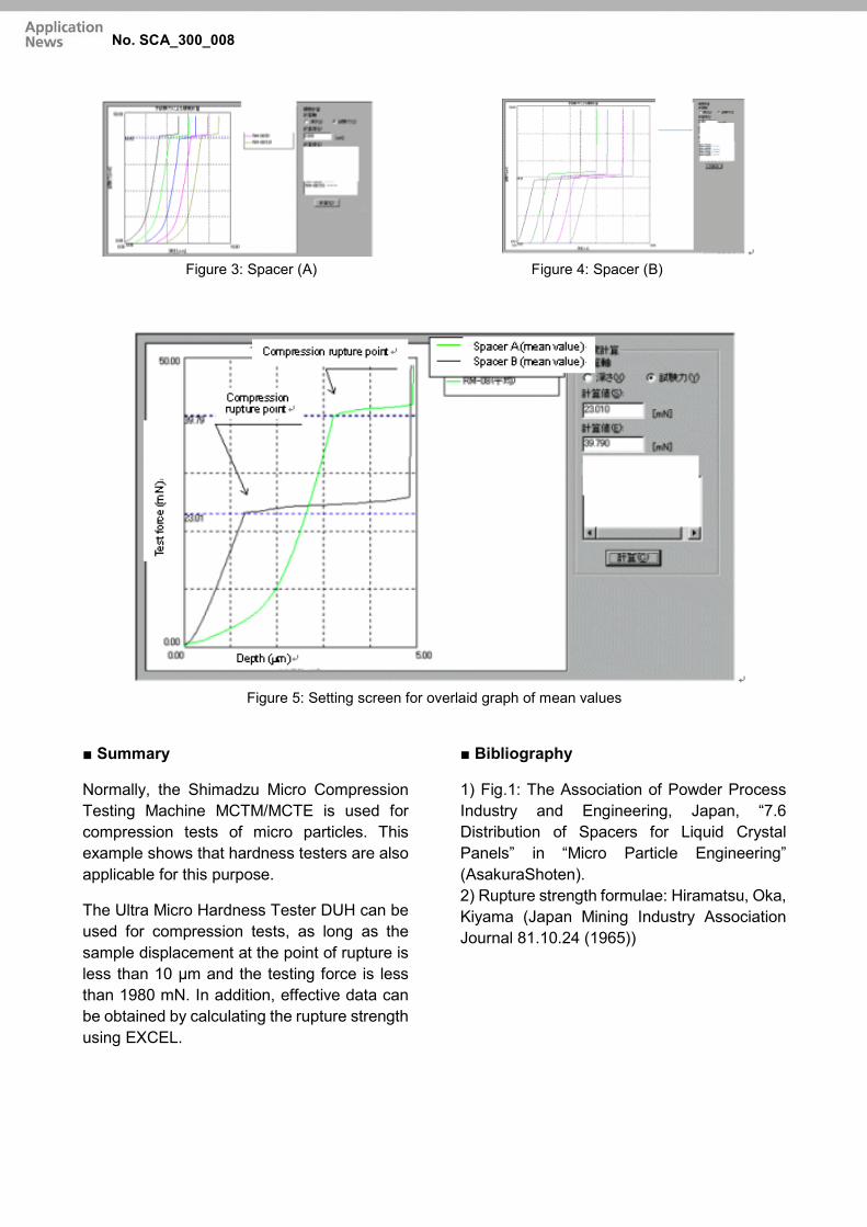
No. SCA_300_008
Figure 3: Spacer (A) Figure 4: Spacer (B)
Figure 5: Setting screen for overlaid graph of mean values
■ Summary
Normally, the Shimadzu Micro Compression Testing Machine MCTM/MCTE is used for compression tests of micro particles. This example shows that hardness testers are also applicable for this purpose.
The Ultra Micro Hardness Tester DUH can be used for compression tests, as long as the sample displacement at the point of rupture is less than 10 µm and the testing force is less than 1980 mN. In addition, effective data can be obtained by calculating the rupture strength using EXCEL.
■ Bibliography
1) Fig.1: The Association of Powder Process Industry and Engineering, Japan, “7.6 Distribution of Spacers for Liquid Crystal Panels” in “Micro Particle Engineering” (AsakuraShoten). 2) Rupture strength formulae: Hiramatsu, Oka, Kiyama (Japan Mining Industry Association Journal 81.10.24 (1965))

No. SCA_300_008
Table 1 Compression test results using DUH Sample name Sample No. Force (N) Particle Diameter
(mm) Rupture strength
(MPa)
Spacer A No. 1 3,979E-02 6,0E-03 985,60 Tube B No. 2 2,301E-02 5,0E-03 820,74
Ref.) Rupture strength was calculated as follows: ST=2,8 P/πd2
ST: Rupture strength (N/mm2 or MPa) P: Test force (N) d: Particle diameter or fiber diameter (mm) Source: Hiramatsu, Oka, Kiyama (Japan Minig Industry Association Journal)
Figure 6: Rupture strength for each spacer
Figure 7: Sample No.1 before and after test
820
985
0
200
400
600
800
1000
1200
No. 1 (Spacer A) No. 2 (Spacer B)
Rupture strength (Mpa)
Particle before test Broken particle after test

■ Introduction A well-known method of testing the hardness of micro diameter wire is to grind the test surface of the wire specimen imbedded in resin and test the cross-section area of the wire. Though the hardness test by imbedding the specimen in resin is reliable, it is not a simple method since it involves imbedding the
specimen in resin and grinding the specimen. The following introduces an example of a hardness test performed using the Shimadzu Dynamic Ultra Micro Hardness Tester without using the resin imbedded method.
■. Specimen
1) Specimen name Extra Fine wire
W SUS
2) Specimen No. No. 1 No.2
3) Wire dia. (μm) ∅20 ∅30
4) Material Tungsten Stainless steel ■ Test Conditions
1) Test Machine
Shimadzu DUH- Dynamic Ultra Micro Hard-ness Tester (See Fig. 1)
2) Indenter Berkovich indenter (made of diamond)
3) Test type Load-unload test 4) Test Force (mN) 9,8 5) Loading Rate
(mN/sec) 0,711
6) Holding Time (sec) 5
7) Test Method
Both ends of the wire were fixed in place on an Si wafer with cellophane tape, and the hardness of the top of the cylindrical part of the wire was tested. (See Fig. 2)
Fig. 1 Overview of DUH
Material Testing System DUH
Hardness Test on Extra Fine Wire by Shimadzu DUH Dynamic Ultra Micro Hardness Tester No. SCA_300_009

No. SCA_300_009
Fig. 2 Conceptual diagram
■ Test results 1) Table 1 summarizes the results (mean
values) of testing by the test conditions in section 2.
.
Table 1 Hardness Measurement Results (Mean Values)
Specimen Name Specimen No. Maximum Force [mN]
Maximum Depth [μm]
Dynamic Hardness
[DHT115-1]
Super-fine wire W No. 1 9,82 0,208 874,717
SUS No.2 9,85 0,243 644,253
Remarks: The calculation expression for dynamic indentation hardness is as follows: DHT115-1 = 3.8584 P/h2 where, DHT115-1 : Dynamic hardness of triangular pyramid indenter at load end P : Maximum Force (mN)
2) Fig. 3 shows the force-depth graph after testing.

No. SCA_300_009
3) The order of specimen hardness in 1) is as follows: No. 1 (tungsten) > No. 2 (stainless steel)
4) Figs. 4 and 5 show images of the
indentation.
■ Summary The Shimadzu DUH-W Dynamic Ultra Micro Hardness Tester allows specimen hardness to be simply evaluated without imbedding the
Indentation
Indentation

No. SCA_300_018
■ Introduction Consumer commodities should measure up to a certain level of quality and function appropriate to their uses. Otherwise, their public reputation may suffer if consumers buy them and they are short of expectations. The Japan Industrial Standard (JIS) sets forth standards specifying quality requirements for products ranging from daily necessities to industrial products. The quality of leads for pencils and automatic pencils is also specified by JIS. It classifies leads in the order of their density and flexural strength, ranging from 9H down to 6B. This standard is used instead of the more reasonable standard of hardness and density because physical calculation of hardness is extremely difficult.
Fig. 1 External View of the DUH-211 Series
The following is an example of hardness measurements performed on pencil leads of different density, a property previously deemed very difficult to measure.
Hardness test on pencil leads (1) Samples Pencil leads of 5H, H, HB, B, 3B, 5B, and red pencil (2) Testing machine (a) Shimadzu Dynamic Ultra Micro Hardness
Tester (b) Standard vise
3) Test result Load versus indenter displacement curves for pencil leads of 5H type and 5B type are shown as examples in Figs.1 and 2 respectively.
Table 1 Testing conditions
10 mgf (for automatic measurement of the indentation depth of an indenter), is applicable to the measurement of the hardness of a wide range of materials from soft materials such as rubbers and plastics to hard materials such as ceramics and diamonds.
TEST MODE 2 CAL. MODE 115° TRIANG. PYRAMID INDENTER MODE AUTO F.S. DEPTH 5 µm MAX LOAD 20 gf LOAD SPEED 0.65 gf/sec
AFTER TIME 5 sec LOT 20 ROOM TEMP 23 – 24 °C
Material Testing System DUH
Hardness Evaluation of Pencil Leads with Shimadzu Dynamic Ultra Micro Hardness Tester No. SCA_300_018

No. SCA_300_018
Fig. 1 Load versus Indentation Depth Curves of Pencil Leads of Type 5H
Fig. 2 Load versus Indentation Depth Curves of Pencil Leads of Type 5B
Note: One of the curves shows an abrupt increase of indentation depths due to internal slipping in the specimen.
Note: Curves exceeding the full scale of 5 μm for indentation depth are shown with the abscissa values deducted by 5 μm.
Table 2 DH Hardness and Flexural Strength of Pencil Leads
Specimen Symbols for density or
color
DH Hardness Flexural strength
Average Standard deviation
Coefficient of variation
kg/m m2
Pencil leads
5H 46.2 4.1 8.8% 7 H 23.9 2.4 9.9% 6
HB 18 2.8 15.5% 5 B 14.9 1.2 8.2% 4 3B 11.9 0.7 5.7% 3 5B 9.5 0.5 5.4% 2
Lead of color pencil Vermilion 6.3 0.4 6.0% 2

No. SCA_300_018
Fig. 3 DH Hardness and Flexural Strength of
Pencil Leads
Table 2 and Fig.3 show a comparison between flexural strengths as specified in JIS S6005-1985 (Leads for pencils, coloured pencils and mechanical pencils) and dynamic hardness calculated from the dynamic indentation depth measured with the Shimadzu Dynamic Ultra Micro Hardness Tester. An appreciably good correlation is observed between flexural strength and dynamic indentation depth. Admitting that there is deviation of data or variation due to different ingredients, this hardness tester is suitable for the quality control of products as long as data is statistically managed.
(Note: For details about hardness of automatic pencil leads, refer to Application News i30)
* Please be advised that data obtained before the implementation of the current Weights and Measures Law may be presented in terms of gravimetric unit.

The hydrogen storage alloy used in fuel cell batteries is generally extremely fragile when compared to the simple metals themselves. Furthermore, as a result of repeated expansion and contraction that occur during hydrogen storage and release, large distortions may be created, finally leading to cracks and pulverization of metal particles. Pulverization causes reduction in the hydrogen storage capacity, deteriorating the original function of the alloy. The following shows an example of hardness measurements that compare the difference of hardness before and after hydrogen storage.
External appearance of DUH
■ Sample 1) Sample name: Hydrogen storage alloy 2) Sample number: No1 (before hydrogen
storage) and No.2 (after hydrogen storage) 3) Sample size: See Fig.1 ■ Test Conditions 1) Testing machine: Shimadzu Dynamic Ultra
Micro Hardness Tester DUH-W201S 2) Indenter: Diamond shaped triangular
indenter with tip angle 115 3) Test mode: Load-unload test 4) Test force: 49 mN 5) Loading rate: 2.684 mN/sec 6) Test force holding time: 10 sec 7). Sample fixing method: Standard vice
Fig.1 Sample Size
Material Testing System MCT
Hardness Measurement of Hydrogen Storage Alloy using the Shimadzu Dynamic Ultra Micro Hardness Tester DUHNo. SCA_300_020

No. SCA_300_020
■ Test Results 1) Table 1 shows the measurement results (mean values) of load-unload tests with the test force of 49 mN. Fig.4 shows the Test force - indentation depth curve. 2) The dynamic hardness DHT115 in Table 1 shows that sample No.1 presents a large hardness than sample No.2 to the separator.
3) As the alloy becomes fragile after hydrogen storage, it was expected that the hardness increases by storing hydrogen. However, the measurements demonstrate the opposite results (see Fig.2 and Fig.3). It is assumed that the cracks caused by hydrogen storage act as springs, making the material appear to be less hard. This assumption requires further examination
Table 1 Hardness measurement results using DUH
Sample Name Sample No. Force Depth
(µm)
Dynamic Hardness (DHT115)
Elastic Modulus (Pa) File Name Figure
Hydrogen storage alloy
Before hydrogen storage
No. 1 49,217 0,537 555,27 1,39E+11 H-01 Fig. 4
After hydrogen storage
No. 2 49,095 0,555 440,84 8,43E+10 H-02
Note: Dynamic Hardness was calculated as follow
𝐷𝐷𝐷𝐷𝐷𝐷𝐷𝐷𝐷𝐷𝐷𝐷115 = 3,8584∙𝑃𝑃𝑃𝑃ℎ2
DHT115: Dynamic hardness by triangular indenter with tip angle 115° P: Test force (mN) H: Indentation depth (µm)
Fig. 2 Sample No. and Dynamic Hardness Fig. 3 Sample No. and elastic modulus
0
100
200
300
400
500
600
No. 1 No. 2
DHT115
DHT115
02468
10121416
No. 1 No. 2
Elastic Modulus
No. 1 No. 2
E+10

No. SCA_300_020
Fig.4 Test Force – Indentation depth curve
■ Summary Hydrogen storage alloys are often used in ways that require repeated storage and release of hydrogen. Lanthanum/nickel alloy, for example, is said to be gradually pulverized while it repeats hydrogen storage and release. In this hardness measurement using the DUH, it has been confirmed that these alloys lose hardness by hydrogen storage.

No. SCA_300_022
■ Introduction The Shimadzu Dynamic Ultra Micro Hardness Tester Model DUH is a machine useful for a very wide range of applications for evaluating the surface hardness of solid samples based on the relation between indenting load and indentation depth. The following presents the results of tests performed on nitrogen ion implanted sintered compact and fly cut platinum and gold specimens. (This data is courtesy of Prof. Kenichi Kanazawa of the Faculty of Machine Engineering, Chiba Institute of Technology, Japan.) ■ Ion implanted alumina ceramics The test piece is a nitrogen ion implanted sintered compact of Al2O3 ceramic. Ion implantation conditions are 90 keV for the accelerating voltage and 2x10¹⁷ ions/cm2 for the quantity of implanted ions. Within the load range below 1 gf, the difference in hardness was significant between the ion implanted specimen and the specimen without ion
implantation, while the difference at the load range of over 1 gf is very small. This demonstrates the effectiveness of this ultra micro hardness tester at load ranges below 1 gf, unavailable to conventional Vickers hardness testers.
Fig.1 Relation between Hardness and Load in Nitrogen Ion Implanted Layer of Ceramic (AL2O3) (with 2x10¹⁷ ions/cm2, triangular pyramid indenter of top angle 100°)
Material Testing System DUH
Hardness Test of Ion Implanted Specimens and Valuable Metals with Shimadzu Dynamic Ultra Micro Hardness Tester Model DUH
No. SCA_300_022
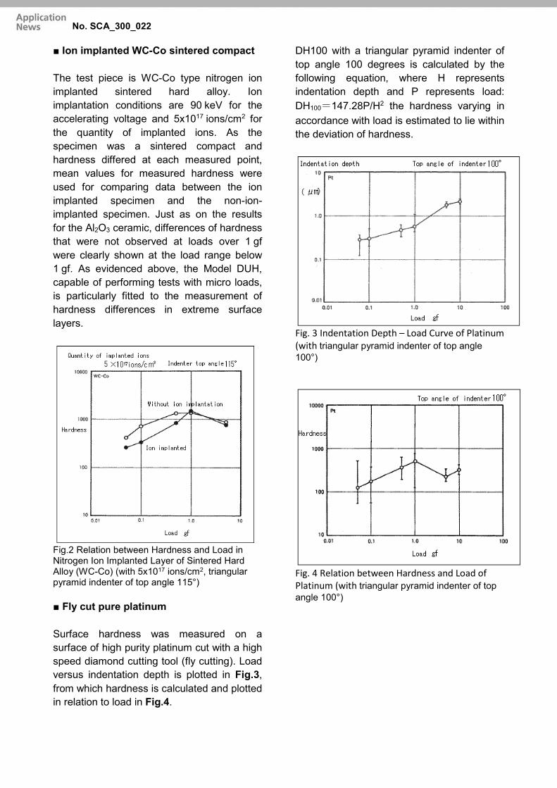
No. SCA_300_022
■ Ion implanted WC-Co sintered compact The test piece is WC-Co type nitrogen ion implanted sintered hard alloy. Ion implantation conditions are 90 keV for the accelerating voltage and 5x10¹⁷ ions/cm2 for the quantity of implanted ions. As the specimen was a sintered compact and hardness differed at each measured point, mean values for measured hardness were used for comparing data between the ion implanted specimen and the non-ion-implanted specimen. Just as on the results for the Al2O3 ceramic, differences of hardness that were not observed at loads over 1 gf were clearly shown at the load range below 1 gf. As evidenced above, the Model DUH, capable of performing tests with micro loads, is particularly fitted to the measurement of hardness differences in extreme surface layers.
Fig.2 Relation between Hardness and Load in Nitrogen Ion Implanted Layer of Sintered Hard Alloy (WC-Co) (with 5x10¹⁷ ions/cm2, triangular pyramid indenter of top angle 115°)
■ Fly cut pure platinum Surface hardness was measured on a surface of high purity platinum cut with a high speed diamond cutting tool (fly cutting). Load versus indentation depth is plotted in Fig.3, from which hardness is calculated and plotted in relation to load in Fig.4.
DH100 with a triangular pyramid indenter of top angle 100 degrees is calculated by the following equation, where H represents indentation depth and P represents load: DH100=147.28P/H2 the hardness varying in accordance with load is estimated to lie within the deviation of hardness.
Fig. 3 Indentation Depth – Load Curve of Platinum (with triangular pyramid indenter of top angle 100°)
Fig. 4 Relation between Hardness and Load of Platinum (with triangular pyramid indenter of top angle 100°)

No. SCA_300_022
■ Fly cut pure gold Just as in the case of platinum, this is a hardness test of fly cut pure gold. As a whole, the deviation of hardness is smaller than that of platinum, suggesting the possibility of hardness testing at a load of as small as 0.01 gf. The indicated hardness is significantly less than that of platinum.
Fig. 5 Relation between Hardness and Load of Gold (with triangular pyramid indenter of top angle 115°)
* Please be advised that data obtained before the implementation of the current Weights and Measures Law may be presented in terms of gravimetric unit.
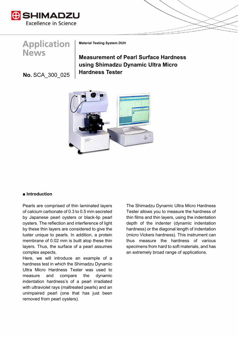
■ Introduction Pearls are comprised of thin laminated layers of calcium carbonate of 0.3 to 0.5 mm secreted by Japanese pearl oysters or black-lip pearl oysters. The reflection and interference of light by these thin layers are considered to give the luster unique to pearls. In addition, a protein membrane of 0.02 mm is built atop these thin layers. Thus, the surface of a pearl assumes complex aspects. Here, we will introduce an example of a hardness test in which the Shimadzu Dynamic Ultra Micro Hardness Tester was used to measure and compare the dynamic indentation hardness’s of a pearl irradiated with ultraviolet rays (maltreated pearls) and an unimpaired pearl (one that has just been removed from pearl oysters).
The Shimadzu Dynamic Ultra Micro Hardness Tester allows you to measure the hardness of thin films and thin layers, using the indentation depth of the indenter (dynamic indentation hardness) or the diagonal length of indentation (micro Vickers hardness). This instrument can thus measure the hardness of various specimens from hard to soft materials, and has an extremely broad range of applications.
Material Testing System DUH
Measurement of Pearl Surface Hardness using Shimadzu Dynamic Ultra Micro Hardness Tester No. SCA_300_025

No. SCA_300_025
Test Conditions Date 28.12.1989
Test Type 2
Speciment No. Pearl
Maximum Load A
Number of repetitions 200,00 gf
Retention Time 1
Pearl 10
File SIN-A2, D1
Indenter DH115
Minimum Load 0,00 gf
Load Speed 1
Deformation Scale
10 μm
Test Conditions Date 28.12.1989
Test Type 2
Speciment No. Pearl
Maximum Load E4
Number of repetitions 200,00 gf
Retention Time 1
Pearl 5
File SINE21, D1
Indenter DH115
Minimum Load 0,00 gf
Load Speed 1
Deformation Scale
10 μm
Fig. 1 Diagram of Load-Indentation Depth Relationship for Unipaired Pearl
Fig. 2 Diagram of Load-Indentation Depth Relationship for Pearl Irradiated with Ultraviolet Rays
Table 1 Hardness of Unimpaired Pearl No. Load (gf) Depth Hardness 1 200,04 7,56 132,4 Average 200,04 7,56 132,4
Table 2 Hardness of Pearl Iradiated with Ultraviolet Rays No. Load (gf) Depth Hardness 1 199,92 13,51 41,45 Average 199,92 13,51 41,45
Table 3 Change in Hardness of Unimpaired Pearl No. Load (gf) Depth Hardness 1 1,720 0,50 260,33 2 5,980 1,00 226,27 3 12,540 1,50 205,84 4 19,780 2,00 187,11 5 29,260 2,50 177,14 6 39,180 3,00 164,70 7 51,980 3,50 160,56 8 64,820 4,00 153,29 9 80,340 4,50 150,12 10 96,760 5,00 146,45 11 115,420 5,50 144,37 12 113,140 6,00 139,94 13 152,280 6,50 136,38 14 173,660 7,00 134,10
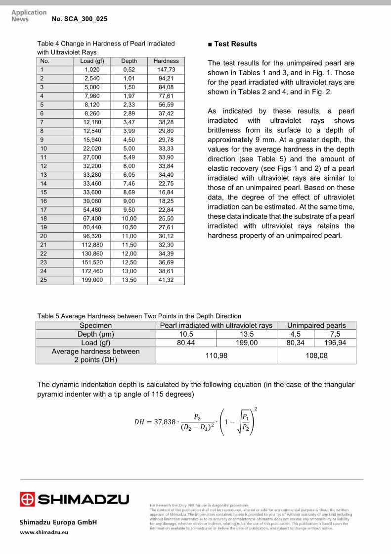
No. SCA_300_025
Table 4 Change in Hardness of Pearl Irradiated with Ultraviolet Rays No. Load (gf) Depth Hardness 1 1,020 0,52 147,73 2 2,540 1,01 94,21 3 5,000 1,50 84,08 4 7,960 1,97 77,61 5 8,120 2,33 56,59 6 8,260 2,89 37,42 7 12,180 3,47 38,28 8 12,540 3,99 29,80 9 15,940 4,50 29,78 10 22,020 5,00 33,33 11 27,000 5,49 33,90 12 32,200 6,00 33,84 13 33,280 6,05 34,40 14 33,460 7,46 22,75 15 33,600 8,69 16,84 16 39,060 9,00 18,25 17 54,480 9,50 22,84 18 67,400 10,00 25,50 19 80,440 10,50 27,61 20 96,320 11,00 30,12 21 112,880 11,50 32,30 22 130,860 12,00 34,39 23 151,520 12,50 36,69 24 172,460 13,00 38,61 25 199,000 13,50 41,32
■ Test Results The test results for the unimpaired pearl are shown in Tables 1 and 3, and in Fig. 1. Those for the pearl irradiated with ultraviolet rays are shown in Tables 2 and 4, and in Fig. 2. As indicated by these results, a pearl irradiated with ultraviolet rays shows brittleness from its surface to a depth of approximately 9 mm. At a greater depth, the values for the average hardness in the depth direction (see Table 5) and the amount of elastic recovery (see Figs 1 and 2) of a pearl irradiated with ultraviolet rays are similar to those of an unimpaired pearl. Based on these data, the degree of the effect of ultraviolet irradiation can be estimated. At the same time, these data indicate that the substrate of a pearl irradiated with ultraviolet rays retains the hardness property of an unimpaired pearl.
Table 5 Average Hardness between Two Points in the Depth Direction Specimen Pearl irradiated with ultraviolet rays Unimpaired pearls
Depth (μm) 10,5 13.5 4,5 7,5 Load (gf) 80,44 199,00 80,34 196,94
Average hardness between 2 points (DH) 110,98 108,08
The dynamic indentation depth is calculated by the following equation (in the case of the triangular pyramid indenter with a tip angle of 115 degrees)
𝐷𝐷𝐷𝐷 = 37,838 ∙ 𝑃𝑃2(𝐷𝐷2 − 𝐷𝐷1)2
∙ (1 − √𝑃𝑃1𝑃𝑃2)2

■ Purpose and Definition Coefficient of friction testing measures the ease with which two surfaces in contact are able to slide over one another. There are two different values associated with the coefficient of friction –static and kinetic (also called dynamic).
■ Equipment used Load cell: 10N, 1/500 Class1 Jig: Friction Modulus Test Device, according to ASTM D1894 Software: Trapezium-X Single / Peel Environment: Room temp 21°C +/-2 °C, humidity ca. 50 +/-5% RH ■ Test jig: The friction jig consists of a fixed 240 x 360 mm, steel, sliding plane which is mounted on the testing machine table with two bolts. The sled, which weighs 200 g and is 63,5 mm x 63,5 mm in size is connected to the load cell with a wire.
Fig. 1 Test Jig
Static friction applies to the force necessary to initialize motion between the two surfaces and kinetic (dynamic) friction is the resistance to moving once the surfaces are in motion over each other. ASTM D1894 is a general standard for Static and Kinetic Coefficients of Friction of Plastic Film and Sheeting which may also be applied on paper and other materials.
Fig.2 Testing Machine
Material Testing System AGS-X
Paper friction test Friction test according to ASTM D1894 No. SCA_300_029

■ Test execution Two samples are prepared, one for the plane and one for the sledge. The plane sample is 250 to 300 mm x 130 mm and is fixed using tape with the short end facing the machine. The sledge is wrapped with the paper sample approx. 63,5 mm wide and long enough to be wrapped around the sled and taped together on top.
Fig.3 Setup 1
When testing card board or other rigid samples they are taped to the bottom side of the sled by using double sided tape. Cleanliness is very important to avoid contaminating the samples with fat or other substances that might affect the friction properties of the sample, gloves may very well be used and the plane should be cleaned using some alcohol based cleaning fluid.
A method is prepared according to ASTM D1894. Test type is single and peel. Test speed is set to 130 mm/min (150 +/-30 mm/min is required.) And stroke limit is set to 130 mm. TrapeziumX is already prepared for this test so the necessary data points for friction, static COF and kinetic COF, are selectable points in the data processing menu. A 50 N load cell was used and all results were below 1N. In this case it is important to set the sensitivity settings very low in the data processing window, default is 1%/FS, and this means that the smallest detectable change would be 0,1 N. The differences between peaks and valleys are about 0,1 N and you might find that no results are presented after the test. This can of course always be adjusted after the test using the re-analyse function.
Fig. 4 Setup 2
No. SCA_300_029

■ Purpose and Definition Tensile tests are a fundamental test within material science and is performed on more or less all materials including paper. Within the paper industry it is very important to know the tensile properties. Paper products are for example often printed in automated machines where the paper is run through big rolls over large distances and at very high speeds. Also in the packaging industry the paper is delivered on big rolls which are then fed into machinery which produce different types of cartons for a great variation of applications and rely on high tensile quality during production. ■ Equipment used Testing machine: EZ-LX Table top Load cell: 1000 N, 1/500 Class1 Jig: PFG-1 kN Pneumatic grips. Software: TrapeziumX Single / tensile. Environment: Room temp 21 °C +/-2 °C, humidity ca. 50 +/-5% RH
Material Testing System EZ-X
Paper Tensile test Tensile test according to ASTM-D 828, EN ISO 1924-2or TAPPI T-494.
No. SCA_300_030

■ Test execution • 5 sets of samples were prepared. • Sample length is 250 mm +/- 5 mm. • Width is 25 mm +/-0,4 mm according to
ASTM D828, (EN ISO1924 width shall be 15 +/-0,1 mm)
• The sample length has to be long enough to allow for 180 mm gauge length, grip separation, and still have enough sample for correct clamping.
• A method is prepared according to ASTM D828.
• Test type is single and tensile. • Test speed is set to 20 mm/min (25 +/-
5mm/min is required according to ASTM and 20 +/-5 mm/min according to EN ISO 1924).
Some data points which may be requested for in this test are: • Tensile strength, kN/m, • Elongation, %, • Tensile energy absorption, J/m2, • Tensile stiffness, kN/m, • Breaking length, m, • Tensile index, Nm/g. • With the help of TrapeziumX and the
calculator in the data processing menu it´s easy to create data points like the ones requested in the paper industry.
No. SCA_300_030

■ Test Results:
Tensile properties are always important in most materials and is the most common test made in universal testing machines. Generally a customer is looking for elastic, maximum and break properties.
Results in this case are presented according to the requirements in ASTM D828. To obtain this result we have a great help from the calculator in TrapeziumX / data processing to present the results in a correct way. Please refer to ASTM D828 for details
Examples of applicable standards: Determination of tensile properties –ISO 1924-2 Tensile Properties of Paper and Paperboard Using ASTM D828 Tensile properties of paper and paperboard TAPPI T-494
No. SCA_300_030

Heat fusing type toner for electronic photographs is used in copying machines and printers of electronic photographing or electrostatic printing type. Toner images are fixed by any one of three methods: by heated roller for melting and fusing toner, by organic solvent for dissolving or softening the binder resin to fix toner, or by pressing toner for fixing. Toners are oriented for use with a particular one of these methods. The most commonly used method at present is the heat roller fusing method, which requires application of heat and pressure simultaneously so that the toner image is in contact with the heated roller and fixed on an imaging sheet. Toners used in this method should be such that they can be fixed at as low a temperature as practicable, and particularly, it should permit quick fixing and a wide range of applicable temperatures. Toners should further agree with such requirements that the image density is good enough to ensure clear images of high resolution and that it allows stable and continuous use at any-time. Toner for electronic photographs comprises binding resin, usually polyester resin, and colouring agents, the softening or melting points of which may be evaluated with the flow tester Model CFT. Thanks to its excellent reputation, the Shimadzu Flow Tester Model CFT is enjoying great demand in the toner industry.
The followings presents an example of viscosity evaluation of a toner for electronic photographs. In general, a flow curve in constant heating rate mode with flow tester Model CFT takes a S-letter shape as shown in Fig. 1. The lower and upper softening temperature limits and point of softening are usually determined from the intersecting points of straight line through the most linear portion of the obtained flow curve with the lines extended from flow starting point and terminating point.
Material Testing System CFT
Viscosity Evaluation of Toner for Electronic Photographs with Shimadzu Flow Tester Model CFT
No. SCA_300_033

Figure 1: Flow curve of toner in constant heating rate mode
■ Flow curve of toner (A) in constant heating rate mode (Figure 2) Test conditions Test temperature: 80 °C to max 300 °C Constant heating rate: 5 °C/min Extruding conditions: Pressure: 50 kgf/cm2 Die: D 0.5 x 1 mm (Diameter x Length)
Figure 2: Flow curve of toner (A) in constant heating rate mode
No. SCA_300_033

■ Flow curve of toner (B) in constant heating rate mode (Figure 3) Test conditions Test temperature: 80 °C to max 300 °C Constant heating rate: 5 °C/min Extruding conditions: Pressure: 50 kgf/cm2, Die: D 0.5 x 1 mm (Diameter x Length)
Figure 3: Flow curve of toner (B) in constant heating rate mode
■ Flow curve of toner (C) in constant heating rate mode Test conditions Test temperature: 80 °C to max 300° C Constant heating rate: 5 °C/min Extruding conditions: Pressure: 50 kgf/cm2, Die: D 0.5 x 1 mm (Diameter x Length)
Figure 4: Flow curve of toner (C) in constant heating rate mode
No. SCA_300_033

High quality printing and copying free from defects like blots is required by the booming office automation movement from which the toner industry is enjoying an increasing demand for toner. Softening temperature and flow properties are the fundamental factors for ensuring the commercial value of toner by quality control.
* Please be advised that data obtained before the implementation of the current Weights and Measures Law may be presented in terms of gravimetric unit.
No. SCA_300_033

During laser printing, toner powder, which has a particle diameter of about 5 μm, is transferred onto copy paper and heated so that it adheres to the paper. In the case of color laser printing, this process is repeated for four different colors. If the melting temperature and melt viscosity differ for the four colors, then it could cause bleeding or poor adhesion in areas printed first and reduce print quality. To prevent that, the temperature characteristics associated with toner flow must be the same for all four colors.
Fig. 1
■ Flow Beginning Temperature for Four Toner Colors by Constant Heating Rate Testing The constant heating rate test was performed for all four color toners used in the same color printer (cyan, magenta, yellow, and black). The constant heating rate method was used to calculate characteristic values such the softening temperature, flow beginning temperature, ½ method temperature, and offset temperature. ½ method temperature: Midpoint between flow beginning and flow ending temperatures Offset temperature: Temperature at flow beginning stroke plus any arbitrary offset stroke. All four toner colors have very similar characteristic values. In particular, the values for the three non-black colors were almost identical. Ensuring that the respective temperature and fluidity characteristics are approximately the same is important for maintaining the print quality of color laser printers. Therefore CFT-EX series flowtesters serve an important role in toner research and development, and quality control applications.
Fig. 2 Stroke- Temperature Graph
Material Testing System CFT
Evaluation of the Temperature Characteristics of Toner No. SCA_300_041

Test Method Constant Temperature Test
DIE Diameter 0,5 mm DIE Length 1 mm Beginning
Temperature 50 °C
Ending Temperature 200 °C Heating Rate 5 °C/min Test Pressure 0,98 MPa
Preheating Time 240 sec Sample Size 1 g (pallets)
Table 1: Test Conditions
Fig. 3 Viscosity-Temperature Graph
Sample Name.
Softening Temperature
(°C)
Flow Beginning Temperature (°C)
½ Methode Temperature
(°C)
½ Methode Temperature
(Pa•s) Cyan 76,8 105,1 132,5 248,2
Magenta 75,4F 105,8 131,8 240,7 Yellow 76,3 104,8 133,5 285,8 Black 73,8 108,5 145,9 402,4
Table 2: Test Result
■ Press-Forming Powdered Samples for Efficient Measurement Due to the small size of toner particles, samples could easily scatter if placed directly in the sample chamber or spill out from die orifices. Therefore, for samples such as these, a hand press and preforming die unit can be used to press them into a form that can be more easily placed in the sample chamber. Accurate values can be measured efficiently by placing only one pellet in the chamber. For thermosetting resin samples, measurements can fail due to ongoing curing during the time it takes to place samples in the sample chamber. Therefore, it is
extremely important to pelletize samples before measurement.
No. SCA_300_041

The Shimadzu Dynamic Ultra Micro Hardness Tester DUH-211S allows hardness measurement with extremely small test force (from 0.1 mN). Therefore, by using this testing machine, characteristics of thin layers can be determined accurately not affected by
the base material. The DUH-211S is being widely used for strength evaluation of various protective layers. The following presents an example where a thin layer (resin layer) on a 6-inch Si wafer was tested for hardness without being broken.
1. Sample
Sample Name Sample No. Thickness Sample size and measurement position
No.1
Si Wafer
No.2
No.3
1. Test conditions
1. Testing machine: Shimadzu Dynamic Ultra Micro Hardness Tester DUH-211S 2. Indenter: Quadrangular pyramid indenter with 136° tip angle (Vickers indenter) 3. Test mode: Load-unload test 4. Test force: 4.9 mN 5. Loading rate: 0.284 mN/sec 6. Load holding time :10 sec
Material Testing System DUH
Hardness Measurement of Thin Layer (Resin Layer) on Si Wafer using the Shimadzu Dynamic Ultra Micro Hardness Tester DUH-211S
No. SCA_300_044

■ Sample fixing method
Sample was fixed by rubber plates and clamps as shown in Fig. 2.
Fig. 2 Sample fixing method diagram
■ Test results
1) Fig.3 shows the “Test force? Indentation depth graph” of the mean values for each sample obtained from hardness measurements.
2) Table 1 shows the results (mean values) of hardness measurements. Dynamic hardness was calculated using the following formula:
DHT115-1 = 3.8584P/D2 DHT115-1: Dynamic hardness measured by triangular indenter with 115° tip angle P: Test force (mN) D: Indentation depth (mm)
3) Measurement results: According to the DHT115-1 values in Table 1, the hardness of the samples is ordered as follows:
No.3 > No.2 > No.1
4) Measurement results: According to the elastic modulus in Table 1, elastic modulus of the samples is ordered as follows:
No.3 > No.2 > No.1
5) For all samples, the elastic modulus decreases with the reduction in hardness.
No. SCA_300_044

Fig. 3 Test Force Indentation Depth Diagram
Table 1 Hardness measurement results ( mean values)
Sample name Sample No.
Dynamic hardness (DHT115-1)
Elastic modulus ( PA ) Data file name
No.1 68 1.12E+10 XX-01
Si wafer resin layer
No.2 111 1.74E+10 XX-02 No.3 176 2.79E+10 XX-03
Ref.) "E+10" in the Elastic modulus columns means 1010
No. SCA_300_044

Fig.4 Sample No. and Dynamic Hardness ( DHT-115-1)
■ Summary
The resin layer on wafer is increasingly resistant to abrasion as the hardness increases, and increasingly strong against damage such as thermal deformation as the
elastic modulus increases. Therefore, layers with high hardness and elastic modulus are desirable, making sample No. 3 the best among the samples tested in this example.
No. SCA_300_044

■ Purpose and Definition All spring manufacturers has to test their type products in quality control and R&D. Tests are performed in tensile or compression direction depending on spring. They have to make tensile tests according to ISO6892 on the spring wire and also tensile or compression tests on the final products. We will have a look at compression tests on helical springs. The results the customers normally are looking for are load at specified height, height at specified load, free height and spring constant. ■ Equipment used Testing machine: AGS-X 5kN Load cell: 1kN, 1/500 Class 1 Jig: Compression plates,
Ø100 mm. Software: Trapezium-X, Spring Environment: Room temp 21°+/- 2 °C,
humidity ca. 50 +/- 5% r.F.
Test jig: Standard compression plates, Ø100 mm 343-08095.
For production control purposes the AGS-X series will be the suitable option. It´s performance and price together with TrapeziumX Spring software makes it a perfect tool for efficient spring testing with high throughput.
Fig. 1. Overview of AGS-X Spring Compression Test
■ Test execution In TrapeziumX, spring we create a method with some typical data points for spring tests. You will find them for example in ASTM A125 where it´s exactly specified what should be selected. We select load at specified Height (LASE), height = spring length. Height at specified load (EASL), free height with a sensitivity (detection point) of 0,01% of full scale (1kN) and spring constant. Free height is the height of the spring at the start of the test and is automatically measured by the instrument. The main difference between a standard compression test and a spring test is that the instrument has to be able to detect the absolute position of the crosshead. This is needed to be able to detect the spring height, which is an important parameter in a spring test.
Material Testing System AGS-X
Spring compression test
No. SEG_300_060

A zero position reset has to be made whenever fixtures are changed or the machine is started. The software will ask for this procedure when started but it has to be done manually by the operator whenever he
changes fixtures (= changes the zero position). The procedure itself is automated and easy to perform and you will be guided by the software.
■ Test Results Spring testing is important for the producer as well as the third party user. Springs are used everywhere and many times in safety functions like spring loaded high pressure release valves.
Height changes at different loads and loads at different heights together with spring constant gives the user or producer important data regarding product quality.
Examples of applicable standards: ASTM A125
No. SCA_300_060

ApplicationNews
No.V20
High-Speed Video Camera
High-Speed Imaging of Laser Ablation Process
LAAN-A-HV-E005
High-Speed Video Camera : Shimadzu Hyper Vision HPV-X2
Lens : 105 mm macro lens
Lighting : Strobe
Recording speed : 10 million frames per second
Target
Base
HPV-X2
StrobeLaser
Laser light
Vacuum chamber
Vacuum chamber
n IntroductionLaser ablation is the process of removing material from a solid (or occasionally liquid) surface by irradiating it with a laser beam. At high irradiation intensities, material on the solid surface is vaporized and converted to plasma. Laser ablation is utilized in a wide range of fields, including product processing, medical, material manufacturing, and more.Examples of product processing include electronic component processing by Q-switched Nd: YAG laser and microfabrication of plastics and ceramics by excimer laser. An example in the medical field is refractive surgery of the cornea using an ArF laser. In material production, it is notably used in thin film production apparatuses. Although this application of laser ablation is not suitable for mass production of thin films, the ability to easily create a thin film having the same composition ratio as a target (solid surface) and the ease with which the thickness can be changed, have led to its wide use in specialized applications. Observation of the substances discharged (plume) during ablation and elucidation of the behavior of the laser ablation plume make it possible to optimize the film-forming conditions and enhance development of thin films. It is believed that observation of the ablation plume using a high-speed video camera is important. Using the Shimadzu Hyper Vision HPV-X2 high-speed video camera, we were able to observe and document the laser ablation plume generated using AZO (transparent electrode material) as the target.
Table 1 Imaging Equipment
n Experimental MethodThe thin film production apparatus consisted of a laser device and a vacuum chamber for ablation. The laser was applied to the target, and film was formed on the substrate above. Fig. 1 shows the state of the experimental apparatus, the vacuum chamber, the Shimadzu HPV-X2, and the target. A target rotation accessory was installed to prevent repeated ablation at the same site on the target. Laser oscillation timing was used as the trigger for recording. Table 1 lists the imaging components.
n Measurement ResultsAs indicated in Table 2, imaging was conducted at a speed of 10 million frames per second. Frame 2 of Fig. 2 shows that laser irradiation has occurred ( indicated by white arrow). Ablat ion occurs in subsequent frames. The intensity of the ablation plume’s emission gradually deteriorates as it spreads in a perpendicular direction to the target.
Table 2 Measurement
Fig. 1 Experiment Equipment
View of entire experimental apparatus (left), vacuum chamber, Shimadzu HPV-X2 (center), and target (right).

ApplicationNews
No.
For Research Use Only. Not for use in diagnostic procedures.The content of this publication shall not be reproduced, altered or sold for any commercial purpose without the written approval of Shimadzu. The information contained herein is provided to you "as is" without warranty of any kind including without limitation warranties as to its accuracy or completeness. Shimadzu does not assume any responsibility or liability for any damage, whether direct or indirect, relating to the use of this publication. This publication is based upon the information available to Shimadzu on or before the date of publication, and subject to change without notice.
© Shimadzu Corporation, 2015www.shimadzu.com/an/
V20
First Edition: Sep. 2015
① ② ③ ④
⑤
⑨ ⑩ ⑪ ⑫
⑬ ⑭ ⑮ ⑯
⑥ ⑦ ⑧
0
50
100
200
250
150
0 5 10 2015Distance from Target (mm)
Brig
htne
ss
Frame②
Frame⑥Frame⑩Frame⑭
Frame③
Frame⑦Frame⑪Frame⑮
Frame④
Frame⑧Frame⑫Frame⑯
Frame⑤
Frame⑨Frame⑬
Fig. 2 High-Speed Images (framing interval: 100 nanoseconds)
Data provided by Kyoto University, Tabe Laboratory
Fig. 3 Brightness of Laser Ablation Plume
Fig. 3 shows the relationship between distance from and brightness of the target vertically. Brightness corresponds to the brightness values obtained by subtracting the brightness of frame 1 (before laser irradiation) from each of the brightness values of frames 2 through 16, respectively. The spreading charac te r i s t i c s o f the ab la t ion p lume can be comprehended from the graph. The speed of the laser ablation plume can be determined based on the 100-nanosecond frame interval.
Note: As the aperture was opened to record the entire ablation, some halation is evident in frames 3 through 7.
n ConclusionLaser ablation is an ultra high-speed phenomenon and can be captured in exquisite detail with the newly developed Shimadzu Hyper Vision HPV-X2 high-speed video camera — featuring recording speeds up to 10 million frames per second and six times higher sensitivity compared to conventional video cameras. Video recording of this type has not been possible using conventional video cameras due to the difficulty of light reaching the target inside the vacuum chamber. The Shimadzu Hyper Vision HPV-X2 high-speed video camera is the best in its class, providing excellent video documentation of the laser ablation process.

ApplicationNews
No.V23
High-Speed Video Camera
Observation of Microbubbles and Cell Behavior Due to Exposure to Ultrasonic Waves
LAAN-A-HV-E008
n Introduction
n Measurement System
One type of drug delivery system (DDS) dosing method involves injecting pharmaceuticals into cells by filling microbubbles with pharmaceuticals, and then collapsing them after making them adhere to cells. In this method, it is important that the drug is injected by penetrating the cell wall, but without killing the cell, as a result of the jet when the microbubble collapses. Accordingly, it is important to observe the behavior of the cell when the bubble collapses. Bubbles are made to collapse by resonance with ultrasonic waves. Resonant frequencies are 1 MHz or higher, so high-speed imaging must be performed at 1 million frames/sec or faster. This article introduces observations of the behavior of cells and microbubbles due to exposure to ultrasonic waves, using the HPV-X2 high-speed video camera.
The HPV-X2 high-speed video camera was used for this experiment. Fig. 1 shows the imaging system, Fig. 2 shows the sample and ultrasonic horn, and Fig. 3 shows a schematic diagram of the imaging system. As in Fig. 2, cancer cells and PVC microcapsules (approximately 5 µm in diameter) are placed in a sample cell filled with physiological saline, which is then placed at the bottom of a water tank. The focus of the ultrasonic horn was aligned with the sample cell, the sample cell was exposed to 1 MHz ultrasonic waves for a total of 3 seconds, and the results were observed with the HPV-X2. The instruments used are indicated in Table 1.
Fig. 2 Sample and Ultrasonic Horn
Fig. 1 Imaging System
Fig. 3 Schematic Diagram of the Imaging System
Table 1 Imaging Equipment
Biological microscope
Sample cell
HPV-X2
Sample cell
Ultrasonic horn
HPV-X2Biological microscope
Sample cell
Horn
Strobe
High-speed video camera : HPV-X2Microscope : IX70 Biological MicroscopeIllumination : Strobe

ApplicationNews
No.
For Research Use Only. Not for use in diagnostic procedures.The content of this publication shall not be reproduced, altered or sold for any commercial purpose without the written approval of Shimadzu. The information contained herein is provided to you "as is" without warranty of any kind including without limitation warranties as to its accuracy or completeness. Shimadzu does not assume any responsibility or liability for any damage, whether direct or indirect, relating to the use of this publication. This publication is based upon the information available to Shimadzu on or before the date of publication, and subject to change without notice.
© Shimadzu Corporation, 2016www.shimadzu.com/an/
V23
First Edition: Mar. 2016
n Measurement ResultsImaging was performed at a speed of 10 million frames/sec. Fig. 4 shows the imaging results. In Image 2 in Fig. 4, the sample is exposed to ultrasonic waves, and the microbubbles within the microcapsules are expanding. The two microbubbles shown by the arrows in Image 3 have made contact with the cell due to the
expansion process and a load is being applied. The expansion of the microbubbles continues until Image 4, after which they contract until Image 11. The cell has become deformed at the two locations shown by the arrows in Image 11, and it can be confirmed that it is damaged.
Fig. 4 High Speed Imaging Results (Interval Between Images is 200 ns)
Data provided by the Laboratory of Biomedical Engineering at Hokkaido University
1 2 3 4
5 6 7 8
9 10 11 12
10 µm
Cell
Microcapsules
n ConclusionThe behavior of cells and microbubbles due to exposure to ultrasonic waves were observed using the HPV-X2 high-speed video camera. Samples were exposed to 1 MHz ultrasonic waves, so an imaging speed of at least 1 million frames/sec was required. Because a microscope was used for imaging, camera sensitivity was very important for these measurements. The newly developed HPV-X2 has at least six times the sensitivity of the conventional HPV-X, so favorable imaging was obtained, even using a microscope, at an imaging speed of 10 million frames/sec. Using the HPV-2 in this way will contribute to DDS development.
Note: Drug Delivery SystemsA drug del ivery system (DDS) i s a system for administering pharmaceuticals. It is a general term for a form of pharmaceutical administration designed to further enhance the effectiveness of medicinal agents, aiming to optimize the pharmaceutical administration route. In other words, the objective is to provide the required pharmaceuticals to the required location at the required time. When medicine is swallowed, only a tiny portion of the amount actually arrives at the affected area to have the intended effect. Some medicinal components are degraded within the body, while others cause side effects by acting at sites where they are not needed. Us ing a DDS enables more effect ive administration, which can be expected to reduce both the dosage of medicinal agents and their side effects, thereby improving the quality of life (QOL) for patients. In addition, expense reductions can be expected due to reductions in the number of times pharmaceuticals are administered.

Founded in 1875, Shimadzu Corporation, a leader in the devel-opment of ad vanced technologies, has a distinguished history of innovation built on the foundation of contributing to society through science and technology. We maintain a global net-work of sales, service, technical support and application cen-ters on six continents, and have established long-term rela-tionships with a host of highly trained distributors located in over 100 countries.
For information about Shimadzu, and to contact your local office, please visit our website at www.shimadzu.eu
Shimadzu Europa GmbHAlbert-Hahn-Str. 6-10 · D-47269 DuisburgTel.: +49 - (0)203 - 76 87-0Fax: +49 - (0)203 - 76 66 [email protected]
![Testing Testing [Read-Only] - Czone - East Sussex](https://static.fdokumen.com/doc/165x107/6327b2a26d480576770d6757/testing-testing-read-only-czone-east-sussex.jpg)