Does a Threshold Inflation Rate Exist?

University of ConnecticutOpenCommons@UConn

Economics Working Papers Department of Economics

December 2007

Quantile Inferences for Inflation and Its Variability:Does a Threshold Inflation Rate Exist?WenShwo FangFeng Chia University

Stephen M. MillerUniversity of Nevada, Las Vegas, and University of Connecticut

Chih-Chuan YehOverseas Chinese Institute of Technology, Taichung

Follow this and additional works at: https://opencommons.uconn.edu/econ_wpapers

Recommended CitationFang, WenShwo; Miller, Stephen M.; and Yeh, Chih-Chuan, "Quantile Inferences for Inflation and Its Variability: Does a ThresholdInflation Rate Exist?" (2007). Economics Working Papers. 200745.https://opencommons.uconn.edu/econ_wpapers/200745

http://lib.uconn.edu/?utm_source=opencommons.uconn.edu%2Fecon_wpapers%2F200745&utm_medium=PDF&utm_campaign=PDFCoverPages

http://lib.uconn.edu/?utm_source=opencommons.uconn.edu%2Fecon_wpapers%2F200745&utm_medium=PDF&utm_campaign=PDFCoverPages

https://opencommons.uconn.edu?utm_source=opencommons.uconn.edu%2Fecon_wpapers%2F200745&utm_medium=PDF&utm_campaign=PDFCoverPages

https://opencommons.uconn.edu/econ_wpapers?utm_source=opencommons.uconn.edu%2Fecon_wpapers%2F200745&utm_medium=PDF&utm_campaign=PDFCoverPages

https://opencommons.uconn.edu/econ?utm_source=opencommons.uconn.edu%2Fecon_wpapers%2F200745&utm_medium=PDF&utm_campaign=PDFCoverPages

https://opencommons.uconn.edu/econ_wpapers?utm_source=opencommons.uconn.edu%2Fecon_wpapers%2F200745&utm_medium=PDF&utm_campaign=PDFCoverPages

https://opencommons.uconn.edu/econ_wpapers/200745?utm_source=opencommons.uconn.edu%2Fecon_wpapers%2F200745&utm_medium=PDF&utm_campaign=PDFCoverPages

Department of Economics Working Paper Series

Quantile Inferences for Inflation and Its Variability: Does a Thresh-old Inflation Rate Exist?

WenShwo FangFeng Chia University

Stephen M. MillerUniversity of Nevada, Las Vegas, and University of Connecticut

Chih-Chuan YehThe Overseas Chines Institute of Technology, Taichung

Working Paper 2007-45

December 2007

341 Mansfield Road, Unit 1063Storrs, CT 06269–1063Phone: (860) 486–3022Fax: (860) 486–4463http://www.econ.uconn.edu/

This working paper is indexed on RePEc, http://repec.org/

AbstractUsing quantile regressions and cross-sectional data from 152 countries, we

examine the relationship between inflation and its variability. We consider twomeasures of inflation - the mean and median - and three different measures ofinflation variability - the standard deviation, coefficientof variation, and mediandeviation. Using the mean and standard deviation or the median and the mediandeviation, the results support both the hypothesis that higher inflation creates moreinflation variability and that inflation variability raisesinflation across quantiles.Moreover, higher quantiles in both cases lead to larger marginal effects of infla-tion (inflation variability) on inflation variability (inflation). Using the mean andthe coefficient of variation, however, the findings largely support no correlationbetween inflation and its variability. Finally, we also consider whether thresholdsfor inflation rate or inflation variability exist before finding such positive corre-lations. We find evidence of thresholds for inflation rates below 3 percent, butmixed results for thresholds for inflation variability.

Journal of Economic Literature Classification: C21; E31

Keywords: inflation, inflation variability, inflation targeting, threshold effects,quantile regression

1. Introduction

Uncertainty emanates from the difficulty of knowing the future values of the variable of interest.

Higher uncertainty reflects higher volatility of the variable’s expected value or a higher variability

of the variable around a given mean. In his Nobel lecture, Friedman (1977) suggests that higher

inflation creates nominal uncertainty, which lowers welfare and output growth. Johnson (1967)

and Okun (1971) argue that although desirable, achieving and maintaining steady inflation proves

problematic because of political factors or policy differences. That is, inflation variability is

unavoidable. Using quantile regression analysis, this paper reexamines empirically the

relationship between aggregate inflation and its variability, especially the issue whether a

threshold inflation rate exists.

The linkages, if any, between inflation and inflation variability received considerable

attention over the past forty years. Friedman (1977) outlines an informal argument regarding how

an increase in inflation raises inflation variability. Ball (1992) formulates Friedman’s hypothesis in

a model of monetary policy, where high inflation creates uncertainty about future monetary policy

and, thus, higher inflation variability. Ungar and Zilberfarb (1993) argue, however, that with rising

inflation agents may invest more resources in forecasting inflation, thus, reducing inflation

variability.

Cukierman and Meltzer (1986), on the other hand, consider the reverse linkage. To wit,

they argue that increases in inflation uncertainty raise inflation by increasing the incentive for the

policy maker to create inflation surprises to stimulate output growth in a game-theory framework.

Thus, inflation variability leads to higher inflation. In contrast, Holland (1995) suggests that higher

inflation variability lowers inflation, if the monetary authorities succeed in stabilizing the

economy.

2

Using annual cross-section data on 17 OECD countries for the period 1951 to 1968, Okun

(1971) reports a positive association between the average inflation rate and its standard deviation,

supporting the Friedman-Ball hypothesis. In a comment, Gordon (1971) notes that the elimination

of the data from the 1950s causes the significant positive correlation to disappear. Logue and

Willett (1976) find similar results for 41 countries across the period 1948 to 1970, but note that this

strong relationship breaks down when disaggregating the sample. Foster (1978) uses average

absolute changes in the inflation rate rather than the standard deviation as a measure of variability

for 40 countries from 1954 to 1975 and obtains results similar to those of Okun (1971) and Logue

and Willett (1976). Davis and Kanago (1998) employ survey data for 44 countries over 20 years,

finding a robust, strong, positive relationship between inflation and its variability across countries,

but the support for Okun’s hypothesis weakens considerably for intracountry data. Similar findings

emerge in Davis and Kanago (2000), who use squared forecast-errors from OECD inflation

forecasts for 24 countries, They find a significant, positive cross-section relationship across

countries between inflation and inflation uncertainty, but the time-series relationship within

countries proves weak, at best. Regarding this weak link at the individual country level, Katsimbris

and Miller (1982) and Davis and Kanago (1996) find, on a country-by-country basis for OECD

and high-inflation countries, a less pervasive, positive relationship between the inflation rate and

its variability than suggested by Okun’s (1971) original findings.

Most recent empirical studies that examine the relationship between inflation and its

variability focus on time-series analysis of a specific economy, since Engle (1982, 1983) applied

the autoregressive conditional heteroskedasticity (ARCH) model to this issue. Inflation variability

decomposes into predictable and unpredictable components. ARCH models estimate the

relationship between inflation and its unpredictable variability, as emphasized by Grier and Perry

3

(1998). This approach produces mixed evidence, however. For example, the Friedman-Ball

hypothesis receives support from Ball and Cecchetti (1990), Grier and Perry (1998), Fountas

(2001), Kontonikas (2004), Conrad and Karanasos (2005), Daal et al. (2005), and Thornton (2007)

for a positive relationship for the G7 and other developed and emerging-market countries. Engle

(1983), Cosimano and Jansen (1988), and Evans (1991) find no support for the hypothesis, where

they focus only on the US.

The Cukierman-Meltzer hypothesis receives support from Baillie et al. (1996) only for a

few high inflation countries. Grier and Perry (1998), Daal et al. (2005), and Thornton (2007) report

mixed evidence to support the hypothesis and even uncover some support for Holland’s counter

hypothesis in developed and developing countries. Hwang (2001) discovers no statistical evidence

for a relationship in the US.

In contrast to time-series tests in individual countries, we apply quantile regressions to the

unconditional inflation and inflation-variability relationships for a cross-section of 152 countries

over 1993 to 2003, returning to the cross-section sampling approach of Okun (1971) and Gordon

(1971). Our cross-section analysis exhibits several differences from previous studies. First, we use

more sample countries. That is, we employ 152 countries as compared to 17 in Okun (1971), 41 in

Logue and Willett (1976), 40 in Foster (1978), 44 in Davis and Kanago (1998), or 24 in Davis and

Kanago (2000). A larger sample size can minimize the chances of spurious results from relatively

few observations.

Second, the sample period of 1993 to 2003 provides analysis for more recent data that

captures several improvements. One, we maximize the number of countries within the sample with

more recent inflation data. Two, the sample period avoids the issue of potential structural change in

inflation variability due to the Great Moderation. That is, inflation increased globally and became

4

more volatile in the 1970s, but since the 1980s, inflation rates fell and became substantially less

volatile, as a pattern across many countries. Three, inflation targeting became an increasingly

popular monetary policy strategy, since New Zealand’s first adoption in 1990. Now, over twenty

countries (industrial and emerging market) target inflation with other countries considering the

possibility. That is, lower inflation, lower persistence, and lower volatility exist in

inflation-targeting countries (Mishkin 1999, King 2002, Mishkin and Schmidt-Hebbel 2007). Our

sample period captures the inflation-targeting era.

Third, we implement quantile regression analysis that permits the calculation of the

cross-sectional correlations between the inflation and its variability at different levels of inflation

and various degrees of variability. This approach to the issues constitutes an innovation in that

prior studies examine Pearson product-moment correlations or ordinary least squares (OLS)

regression analysis. Moreover, conventional cross-section studies examine the Friedman-Ball or

Okun hypothesis only. The present paper considers the Cukierman-Meltzer hypothesis as well.

Fourth, we introduce two measures of inflation – the mean and median – and three

measures of its variability – the standard deviation, coefficient of variation, and median

deviation – to examine the robustness of the relationships, if any. The positive correlation does not

prove robust across the different measures of level and variability.

Finally, Davis and Kanago (1998, 2000) note that some researchers (Logue and Willet,

1976 and Hafer and Heyne-Hafer, 1981) find that the positive correlation between inflation and its

variability does not hold for low inflation countries. Logue and Willett (1976) report insignificant

correlation for highly industrialized countries or for those with modest inflation rates between two

to four percent over the period 1948-1970.1 Hafer and Heyne-Hafer (1981) conclude that the

1 Gale (1981) reports that a clerical error may explain the insignificant correlation for industrialized countries in the

5

threshold level of inflation above which the positive correlation emerges rose from around 4

percent for data in the 1950 to 1970 sample period to around 9 percent for their sample from 1970

to 1979. We split the sample into two different sets of sub-samples. First, we split the sample at the

median (i.e., just over 6 percent) and show that, across countries, a significant positive relationship

exists between the mean inflation rate and its variability, for both low and high inflation countries.

That is, we reject the notion of a threshold effect at 6 percent. Moreover, we find that frequently the

marginal effects prove larger for low inflation countries. Second, we split the low inflation sample

(i.e., countries less than the median) at its median (i.e., just under 3 percent), creating low and

moderate inflation countries. Now, the low inflation countries do not exhibit the positive

correlation between inflation variability and its level.

We also split the sample of countries into two different sets of sub-samples based on the

inflation variability. First, we split the sample at the median (i.e., just over 4.25 percent) and show

that, across countries, a significant positive relationship exists between the inflation variability and

its mean, for both low and high inflation variability countries. That is, we, once again, reject the

notion of a threshold effect. Moreover, we find that the marginal effects prove larger for low

inflation variability countries. Second, we split the low inflation variability sample (i.e., countries

less than the median) at its median (i.e., just under 1.75 percent), creating low and moderate

inflation variability countries. Now, the low and high inflation variability countries exhibit mixed

findings. Sometimes a positive relationship exists for some quantiles while for other quantiles no

relationship exists.

Quantile regression, developed by Koenker and Bassett (1978) and popularized by

Buchinsky (1998), extends estimation of ordinary least squares (OLS) of the conditional mean to

1949 to 1970 sample.

6

different conditional quantile functions. Conditional quantile regressions minimize an

asymmetrically weighted sum of absolute errors. Many areas of applied econometrics -- such as

investigations of wage structure, earning mobility, educational attainment, value at risk, option

pricing, capital structure, and economic development – now employ quantile regressions for some

of its empirical work. Koenker (2000) and Koenker and Hallock (2001) provide an excellent

discussion of the intuition behind quantile estimators and various empirical examples.

We provide the first application of the quantile regression method to cross-country

relationship between inflation and its variability. Our empirical findings support both the

Friedman-Ball and Cukierman-Meltzer hypotheses when we use the mean and the standard

deviation of inflation or the median and the median deviation. Moreover, higher inflation and

higher inflation variability exhibit larger marginal effects. Using the measure of mean inflation and

the coefficient of variation, however, such correlation disappears. In sum, the positive correlation

between inflation and its variability does not prove robust to alternative definition of inflation and

its variability. Finally, using the mean and its standard deviation, we also find evidence of

threshold effects for inflation rates under 3 percent. But, we do not find consistent evidence of a

threshold effect for the effect of inflation variability on inflation.

The rest of the paper flows as follows. Section 2 presents a brief review of the quantile

regression method and its properties. Section 3 discusses the data and the results. Section 4

considers the possibility of threshold effects. Section 5 concludes.

2. Quantile regressions in inflation and inflation variability

Quantile regression is outlined as follows:

i iy x u iτ τβ′= + and (1)

( )i i iQuantile y x xτ τβ′= , (2)

7

where yi equals the dependent variable (i.e., inflation or inflation variability), equals a vector of

independent variables (i.e., inflation variability or inflation, respectively), β

ix′

τ equals the vector of

parameters associated with the quantile (percentile), and uthτ τi equals an unknown error term.

Unlike ordinary least squares (OLS), the distribution of the error term uτi remains unspecified in

equation (2). We only require that the conditional quantile of the error term equals zero, that is, thτ

( ) 0i iQuantile u xτ τ = . ( )i i iQuantile y x xτ τβ′= equals the thτ conditional quantile of y given x

with (0,1)τ ∈ . By estimating βτ, using different values of τ , quantile regression permits different

parameters across different quantiles of inflation or inflation variability. In other words, repeating

the estimation for different values of τ between 0 and 1, we trace the distribution of y conditional

on x and generate a much more complete picture of how explanatory variables affect the dependent

variable.

Furthermore, instead of minimizing the sum of squared residuals to obtain the OLS (mean)

estimate of β, the quantile regression estimate βthτ τ solves the following minimization problem:

{ : } { : }

2 2(1 )mini i i i

i i i ii i y x i i y x

y x y xβ β β

τ β τ′ ′∈ ≥ ∈ <

⎡ ⎤β′ ′− + − −⎢ ⎥

⎣ ⎦∑ ∑ . (3)

That is, the quantile approach minimizes a weighed sum of the absolute errors, where the weights

depend on the quantile estimated. Thus, the estimated parameter vector remains less sensitive to

outlier observation on the dependent variable than the ordinary-least-squares method. The solution

involves linear programming, using a simplex-based algorithm for quantile regression estimation

as in Koenker and d’Orey (1987). The median regression occurs when 0.5τ = and the coefficients

of the absolute values both equal one.2 When 0.75τ = , for example, the weight on the positive

2 That is, the least or minimum absolute deviation (LAD or MAD) estimator occurs with τ = 0.5. We insert the twos so that the value of the function equals the LAD or MAD function value when τ = 0.5. Some references exclude the twos,

8

errors equals 1.5 and the weight on the negative errors equals 0.5, implying a much higher weight

associates with the positive errors and leads to more negative than positive errors. In fact, the

optimization leads to 75-percent (25-percent) of the errors less (greater) than zero.

One additional comment distinguishes quantile regression from within quantile OLS

regressions. That is, some analysts think that results similar to quantile regression occur when one

segments the dependent variable’s unconditional distribution and then uses OLS estimation on

these subsamples. Koenker and Hallock (2001) argue that such “truncation on the dependent

variable” generally fails precisely because of the sample selection issues raised by Heckman

(1979).

To conduct parameter tests, we employ the design matrix bootstrap method to obtain

estimates of the standard errors, using STATA, for the parameters in quantile regression

(Buchinsky, 1998). In every case, we use 10,000 bootstrap replications. This method performs

well for relatively small samples and remains valid under many forms of heterogeneity. More

conveniently, these bootstrap procedures can deal with the joint distribution of various quantile

regression estimators, allowing the use of the F-statistic to test for the equality of slope parameters

across various quantiles (Koenker and Hallock, 2001).

We estimate the following two simple linear quantile regression models:

iV i iτ τ τγ δ ν= + ∏ + and (4)

i iV u iτ τ τα β∏ = + + , (5)

where equals the measure of the inflation-rate variability – the standard deviation, coefficient

of variation, or median deviation -- over 1993 to 2003,

iV

i∏ equals the measure of the inflation

since the estimates prove invariant to its inclusion or exclusion.

9

rate – mean or median -- over 1993 to 2003, τγ , τδ , τα , and τβ equal unknown parameters that are

estimated for different values of τ , and iτν and iuτ equal the random error terms. By varying τ

from 0 to 1, we trace the entire distribution of inflation variability (or inflation), conditional on

inflation (or inflation variability). Friedman and Ball predict that δτ > 0 and Cukierman and

Meltzer, that βτ > 0.

3. Data and empirical results

Annual inflation rates equal the percentage change in the logarithm of consumer price index (base

year in 2000) gathered from the International Monetary Fund (IMF) International Financial

Statistics for 152 countries from 1993 to 2003. We proxy the inflation-rate variability by the

standard deviation, coefficient of variation, or median deviation of the inflation rate.3 Average and

median values of the inflation rates and the three measures of the inflation rate variability in each

country comprise 152 sample observations. Table 1 presents the summary statistics as well as

statistics for the five countries with the highest and lowest mean and median inflation rates. Both

the mean and the median exhibit highly right-skewed distributions with outliers, as evidenced by a

larger mean than the median. Quantile regression proves robust to departures from normality with

skewed tails.

Geometrically, the mean of a variable equals its center of gravity. In Table 1, the mean

inflation ranges from 0.1341 percent in Japan to 68.6939 percent in Turkey, and responds

significantly to extreme values. The highly skewed distribution (skewness=2.3257) suggests that

the median may provide a better alternative to measure central location. The median, a positional

3 We note that inflation variability measured by the standard deviation will equal inflation uncertainty, when the expected inflation rate of the sample period equals the average inflation rate over that period. That is, inflation uncertainty typically equals the variability of the actual inflation rate around its expected value. So, if average inflation equals the expected inflation, then the standard deviation of the inflation rate will equal the inflation uncertainty as well.

10

value, divides the observations on the inflation rate into two equal parts. It does not equal the mean,

and does not respond to extreme values. Different measures of inflation and its variability, that is,

the mean and standard deviation versus the median and median deviation, should not influence the

relationship between the two variables for a robust relationship. Additionally, in Table 1, the five

countries with the highest inflation rates face higher standard deviations, while countries with the

lowest inflation rates face lower standard deviations. The mean value also influences its standard

deviation. To avoid this issue, we also consider the standard deviation of the mean or the

coefficient of variation to measure variability in our analysis.

Table 2 presents results of estimating the Friedman-Ball hypothesis with quantile

regressions, using the mean and standard deviation of the inflation rate, for τ = 0.05, 0.25, 0.50,

0.75 and 0.95, an OLS regression, and F-statistics testing for equality of the estimated slope

parameter between various quantiles. The homogeneity test considers whether the five slope

coefficients equal each other across the five quantiles. Such tests provide a robust alternative to

conventional least-squares-based test of heteroskedasticity, because we can construct them to

remain insensitive to outlying response observations. The OLS regression results show that higher

inflation creates more inflation variability, which closely coincides with Friedman’s (1977)

argument that “the most fundamental departure is that…the higher the (inflation) rate, the more

variable it is likely to be.” (p. 465). The quantile regression results illustrate that the marginal

effect of inflation on inflation variability increases as one moves from lower to higher inflation

variability quantiles. That is, with a higher inflation variability quantiles, inflation exerts a larger

effect on inflation variability. This evidence suggests that potential information gains associate

with the estimation of the entire conditional distribution of the variable concerned, as opposed to

the conditional mean only.

11

More specifically, the OLS regression generates positive and significant coefficients of

inflation at the 1% level, supporting the Friedman-Ball hypothesis that inflation generates inflation

variability. The five-quantile regression estimates of inflation, conditional on inflation variability,

all prove positive and significant at the 1% level. Moreover, higher quantiles associate with a

larger coefficient. In the bottom panel of Table 2, significant F-statistics suggest that inflation

affects inflation variability differently across the distribution of inflation uncertainty, except

between the 0.50th and 0.95th, and 0.75th and 0.95th quantiles. In addition, the homogeneity test

rejects the null hypothesis that all five slope coefficients equal each other. Inflation exhibits a

larger effect on inflation variability for the upper tail distribution of inflation uncertainty than the

lower tail. Moreover, the intercept term does not change across quantiles and does not differ

significantly from zero, except at the 25th and 50th quantiles. The evidence supports the

Friedman-Ball hypothesis.

Figures 1 and 2 illustrate the findings. Figure 1 shows that the quantile regression lines

rotate to a higher slope with a relatively constant intercept as the estimates move from lower to

higher quantiles. Figure 2 reinforces Figure 1, plotting the slope coefficient with 5-percent

significance bands, where the horizontal dashed line represents the OLS estimate. The slope

coefficient starts below the OLS estimate for low quantiles and rises above the OLS estimate for

high quantiles.

Table 3 reports the results of estimating the Cukierman-Meltzer hypothesis, using the mean

and standard deviation of the inflation rate. All estimates of inflation variability prove positive and

significant at the 1% level. In addition, the marginal effects of inflation variability on inflation rise

significantly across quantiles except at the 0.95th quantile tail, as the F-statistics, testing for

equality of slope estimates across quantiles, demonstrate. In addition, the homogeneity test, once

12

again, rejects the null hypothesis that all five slope coefficients equal each other. In addition, the

intercept term, which proves significantly positive, increases significantly across quantiles. That is,

the evidence supports the Cukierman-Meltzer hypothesis.

Figures 3 and 4 illustrate the findings. Once again, the quantile regression lines rotate to a

higher slope with a relatively constant intercept as the estimates move from lower to higher

quantiles. The slope coefficient also starts below the OLS estimate for low quantiles and rises

above the OLS estimate for high quantiles.

Tables 4 and 5 report the quantile estimates for the Friedman-Ball and Cukierman-Meltzer

hypotheses, using the mean and coefficient of variation of the inflation rate. The OLS regressions

do not find a significant relationship between inflation and its variability, or vice versa. Rather, the

constant terms prove significant. Examining the quantile results, inflation positively affects

inflation variability at the 25th and 50th quantiles in Table 4, but the coefficients prove small in

magnitude. Similarly, inflation variability negatively affects the inflation rate at the 5th and 95th

quantiles in Table 5.4 Finally, the constant terms rise across the quantiles as expected when the

slope coefficient does not generally prove significant. Thus, the use of the coefficient of variation,

rather than the standard deviation, eliminates the significance of the Friedman-Ball and

Cukierman-Meltzer hypotheses in the OLS specifications. The quantile findings provide weak

support for the Friedman-Ball hypothesis, but weak support for reversing the Cukierman-Meltzer

hypotheses to a negative effect. Thus, our empirical results show that the widely agreed positive

association between inflation and its dispersion do not prove robust to the relative measure. Thus,

4 The F-statistics testing for the equality of the slope coefficients across quantiles cannot reject equality, except for the 95th quantile in the Friedman-Ball model. Here, the slope coefficient proves significantly different from those at the 5th, 25th, 50th, and 75th quantiles at the 1-, 5-, or 10-percent levels. At the same time, the slope coefficient at the 95th quantile does not prove significantly different from zero, however. Furthermore, the homogeneity test cannot reject the null hypothesis that all five slope coefficients equal each other.

13

this study raises one issue that deserves further attention: which measure more appropriately

captures variability -- absolute or relative dispersion.

Traditionally, researchers use the standard deviation, based on deviations from the mean, to

measure dispersion in the inflation rates. This absolute deviation measure proves misleading when

some data exist far away from the mean, such as the inflation rates of the five highest and lowest

countries reported in Table 1. We may conclude that more dispersion exists in the inflation rates of

the higher mean inflation countries because of their much higher standard deviations, since the

means are so far apart. When we convert the statistics to coefficients of variation, less variations in

four of the five highest mean inflation countries occurs. For example, the standard deviation of the

mean equals 6.4228 in Japan, the country with the lowest inflation rate in our sample, and only

0.3361 in Turkey, the one with the highest rate. The relationship between inflation and its

variability in high- or low-inflation countries cannot be seen simply as shown by the statistics.

Alternatively, what explains this change in findings? Intuitively, it implies that the

variability of a series rises proportionately with the mean of the series, leading to no correlation

between the mean and its coefficient of variation. To get a positive correlation between the mean

and its coefficient of variation, the variation of the series must rise more than proportionately with

the mean and median. Viewed differently, we can convert the Friedman-Ball specification with the

standard deviation and mean into the specification with the coefficient of variation and the mean

by dividing the initial specification by the mean inflation. Thus, one gets the following outcome:

1 .i

i i

V i

i

ττ τ

νγ δ= + +∏ ∏ ∏

(6)

Thus, the intercept term in the Freidman-Ball regression with the coefficient of variation as the

dependent variable (i.e., τδ ) approximates the slope coefficient in the Friedman-Ball specification

with the standard deviation as the dependent variable. Moreover, the slope coefficient in the

14

Freidman-Ball regression with the coefficient of variation as the dependent variable (i.e., τγ )

approximates with the opposite sign the intercept term in the Friedman-Ball specification with the

standard deviation as the dependent variable. 5 Comparing Tables 2 and 4, we see the

correspondence.

Figures 5, 6, 7, and 8 illustrate the findings. Here, the slope coefficients generally prove

insignificant and the movements in the quantile regression lines largely reflect changes in the

intercepts.

Tables 6 and 7 report the quantile estimates for the Friedman-Ball and Cukierman-Meltzer

hypotheses, using the median and median deviation of the inflation rate. The OLS regressions find

a significant positive relationship between inflation and its variability, the same as using the mean

and standard deviation of the inflation rate in Table 2. Moreover, inflation significantly affects

inflation variability at each of the quantiles.6 In addition, the constant terms prove significantly

positive at the higher tails of 75th and 95th. Similarly, inflation variability significantly affects the

inflation rate at each of the quantiles matching the findings in Table 3.7 Finally, the pattern in the

intercepts matches the pattern seen in Tables 2 and 3. Thus, the use of the median and the median

deviation produces a positive correlation, supporting the Friedman-Ball and Cukierman-Meltzer

hypotheses and matching the findings for the mean and standard deviation. The quantile findings

confirm a positive relationship.

5 These comments, of course, ignore issues related to the new error term in the transformed model. 6 The F-statistics testing for the equality of the slope coefficients across quantiles rejects equality for the 75th and 95th quantiles relative to the 5th, 25th, and 50th quantiles in the Friedman-Ball model at the 1-, 5-, or 10-percent levels. In addition, the homogeneity test rejects the null hypothesis that all five slope coefficients equal each other. 7 The F-statistics testing for the equality of the slope coefficients across quantiles rejects equality for the 75th and 95th quantiles relative to the 5th and 25th quantiles in the Cukierman-Meltzer model at the 1-, 5-, or 10-percent levels. In addition, the homogeneity test, once again, rejects the null hypothesis that all five slope coefficients equal each other.

15

Figures 9, 10, 11, and 12 illustrate the findings. We return to the situation where the

quantile regression lines rotate to a higher slope with a relatively constant intercept as the

estimates move from lower to higher quantiles. Moreover, the slope coefficient, once again, start

below the OLS estimates for low quantiles and rise above the OLS estimates for high quantiles.

4. Does a Threshold Inflation Rate Exist?

Most researchers find a positive relationship between inflation and its variability across countries.

A few authors, however, do find that for low inflation countries, the positive relationship does not

prove significant (Logue and Willet, 1976 and Hafer and Heyne-Hafer, 1981). This section

explores the issue of whether a threshold level of inflation exists before finding the positive

correlation between inflation and its variability. The analysis considers the Friedman-Ball and

Cukierman-Meltzer hypotheses using only the mean and standard deviation of the inflation rate.

That is, we must consider a specification for which we find a positive correlation in order to

determine if a low-inflation threshold exists.

The Appendix Table reports the average annual inflation over 1993 to 2003 for all 152

countries. Generally, developed and developing countries exhibit low average inflation rates, other

countries, which do not develop over time, exhibit high inflation rates. We split the full sample into

two sub-samples, low-inflation countries and high-inflation countries, at the median inflation (i.e.,

6.1471 percent), and test for the equality of the relationship between mean inflation and its

standard deviation for each sub-group (76 countries in each group), using the dummy-variable

technique.8 That is, we define a dummy variable as D=1 for the high-inflation countries and 0

otherwise in the Friedman-Ball regression model as follows:

8 The dummy-variable approach has an advantage over splitting the sample of the Chow test, namely, we can individually test the intercept or slope of the regression coefficients for equality (or structural change) rather than the entire relation.

16

(i D i D iV D Dτ τ τ τ ) .iγ γ δ δ= + + + Π (7)

The estimated individual models bifurcate as follows:

iDDiV Π+++= )ˆˆ(ˆˆˆ ττττ δδγγ , (high-inflation countries), and (8)

iiV Π+= ττ δγ ˆˆˆ , (low-inflation countries). (9)

Testing whether Dτγ or Dτδ prove significant will determine whether the intercept or the

slope differ between the high- and low-inflation countries. The null hypothesis Dτγ = Dτδ = 0

indicates that no structural change occurs between the two groups. Table 8 reports each of the tests

using the mean and standard deviation of the inflation rate, with p-values in parentheses. In the

OLS regression, the insignificant intercept dummy estimate and the significant interaction term

imply that no significant difference exists in the intercept between the high- and low-inflation

countries, but a significant difference does exist in the slope coefficients. Moreover, the significant

F-statistic rejects the null hypothesis of no structural change (i.e., Dτγ = Dτδ = 0), suggesting that

on the average, the high inflation countries exhibit a different response to variability than the low

inflation countries. For the quantile regressions, although the individual estimates of Dτγ and Dτδ

prove insignificant in all five quantiles, except the intercept dummy in the 25th quantile, the

significant F-statistics, however, unanimously reject the joint test of equality, suggesting

difference in the relationship between the high- and low-inflation countries. Generally, the power

of a joint test is stronger than that of an individual test.

Panels A and B of Table 9 present the results of estimating the Friedman-Ball hypothesis

from the high- and low-inflation country samples, respectively.9 All slope parameters of inflation

9 Precisely the same results emerge from Tables 8 and 9. We provide Table 9 so that the reader can more easily see the relationships between the models for low- and high-inflation countries. Also in the process, elimination of the insignificant dummy variable leads some estimates to become significant.

17

in the OLS and quantile regressions prove positive and significant. Also, the slope parameter rises

as we move from lower to higher quantiles. That is, for the Friedman-Ball hypothesis, the same

basic pattern of effects occurs across the quantiles for the high and low inflation country samples.

Moreover, the slope parameters at the 0.5th, 0.75th, and 0.95th quantiles in the high-inflation

countries (Panel A) appear less than those in the low-inflation countries (Panel B).

This decomposition of our 152-country sample at the median inflation rate shows that

inflation variability and the level of inflation positively relate across countries in each group. Thus,

no evidence of a threshold effect emerges from this analysis. Policymakers may want to know the

inflation rate above which significant increases in variability occur, lowering welfare and output

growth. Previous studies provide only limited and mixed evidence on the sensitivity of inflation

variability to its level in high-, low-, or moderate-inflation regimes. Logue and Willett (1976) find

insignificant correlation for countries with moderate inflation between two to four percent. Hafer

and Heyne-Hafer (1981) discover the upper bound of the threshold increases sharply from four to

nine percent in the 1970s. Ram (1985) argues that although the average inflation rate rises during

the 1970s, the level-variability correlation falls in the 1970s. Moreover, a significant positive

correlation emerges only when inflation rates exceed eight percent in the 1960 to 1970 sample and

twenty percent in the 1972 to 1981 sample. Edmonds and So (1993) discover significant

relationships for a group of high- and low-inflation countries, but not for a group of

moderate-inflation between six and ten percent. Hess and Morris (1996), on the other hand,

demonstrate a significant positive relation for countries with low- and moderate-inflation less than

fifteen percent a year. Davis and Kanago (1996) find a significant positive relation in ten high

inflation countries, however, the coefficients are no longer significant when David and Kanago

(2000) restrict OECD countries with inflation under eight percent.

18

How low (moderate or high) is a low (moderate or high) inflation rate? No theory or

empirical analysis gives a definite answer. That is, although sample dates, countries, measures of

variability, and sources of data may lead to different results, the relevant policy question for most

industrialized countries and many emerging market countries in recent years concerns the benefits

from reducing inflation from high or moderate levels to low levels. Our sample period, 1993-2003,

encompasses the inflation-targeting era and the period of the Great Moderation. Thus, we search

for a threshold level of inflation, if any, based on the inflation targets adopted by inflation-targeting

countries. Inflation targeting provides an operational framework for monetary policy to attain

price stability. Typically, inflation targets correspond to an annual rate of inflation in the low single

digits (Bernanke et al. 1999, Batini and Yates 2003). Table 10 (International Monetary Fund 2005)

lists 21 countries that use inflation targets, their inflation-targeting adoption years and their current

inflation targets. The Table includes 8 industrial countries and 13 emerging market countries.

The numerical inflation target typically reflects an annual rate for the CPI in the form of a

range, such as one to three percent (e.g., New Zealand and Canada). Alternatively, the inflation

rate target equals a point target with a range, such as a two-percent target plus or minus one

percent (e.g., Sweden) or a point target without any explicit range, such as a two-percent target

(e.g., the United Kingdom). For industrial countries, the targets range between zero and three

percent. For emerging market countries, they all adopt a target range or a point target with a range.

The middle of the range or the point target generally exceeds that in the industrial countries. The

range runs from zero and six percent (except for seven percent in Brazil), which nearly matches the

range from zero to median inflation rate (6.1471 percent) in our sample. We saw in Panel B of

Table 9 that inflation variability positively and significantly relates to the inflation rate for the

sample of inflation rates between zero and 6.1471 percent. The practice of inflation targeting in the

19

world leaves open the question of whether inflation variability differ in high or low

inflation-targeting regimes, even at the already lower level of inflation. Thus, we further break our

sample at a lower inflation rate to look for a threshold. An examination of our sample data, the

median inflation of our 76 low-inflation countries (or, equivalently, the 25 percent of our 152

countries) equals 2.9349 percent, which matches the edge of the three percent rate target for the

industrial countries. We, thus, split our 76 low-inflation countries at its median inflation (2.9349

percent) into two groups (38 countries in each) – low and moderate inflation rate countries. Table

11 reports the estimation results, where the dummy variable D=1 for the moderate-inflation

countries and 0 otherwise, testing for equality of estimates between the two regimes.

In the OLS regression, although Dτγ or Dτδ do not test significantly different from zero,

the F-statistic significantly rejects the null hypothesis of equality (i.e., Dτγ = Dτδ = 0), suggesting

that the countries with moderate inflation rates (i.e., three to six percent) exhibit different behavior

from the countries with low inflation rates (i.e., zero to three percent). All the quantile regressions

strongly support this conclusion. Four estimates of Dτγ and two estimates of Dτδ prove significant

in the five quantiles and the significant F-statistics reject the joint test of equality for all five

quantiles. Generally, we conclude that differences exist in the relationship between the moderate-

and low-inflation countries.

Panels A and B of Table 12 present the estimation results from the moderate- and

low-inflation country samples, respectively. In Panel A, for the moderate-inflation countries, all

slope parameters of inflation in the OLS and quantile regressions prove positive and significant,

except at the 0.50th quantile. That is, the Friedman-Ball hypothesis holds in countries with

moderate inflation rates. In Panel B for the low-inflation countries, however, all slope parameters

in the OLS and quantile regressions appear insignificant, except at the 0.05th quantile, where

20

marginal effect of inflation proves much lower than the similar effect in the moderate countries. In

sum, different effects occur across quantiles for the moderate and low inflation country samples.

Considerable evidence exists that inflation and its variability positively correlate across

countries. Our findings demonstrate that a threshold level of inflation does exist before the positive

correlation emerges. The threshold occurs around the three percent inflation rate. Countries with

inflation rates below the threshold, such as those industrial countries adopting and achieving

inflation targets of less than three percent, generally find no association between inflation and its

variability. Countries that achieve their inflation rate targets above the threshold, such as most

emerging market countries, face the fact that higher inflation associates with higher inflation

variability. This evidence suggests that if the authorities want to eliminate the uncertainty of

inflation, then inflation targets must not exceed the threshold of three percent.

Similar evidence emerges when estimating and testing the Cukierman-Meltzer hypothesis.

In this case, we split the full sample at the median standard deviation (i.e., 4.3639 percent) into two

sub-samples, low- and high-inflation-variability countries. Thus, we define a dummy variable as

D=1 for high-inflation-variability countries and 0 otherwise in the Cukierman-Meltzer regression

model as follows:

iiiDiDi uVDD τττττ ββαα ++++=Π )( . (10)

The estimated individual models bifurcate as follows:

iDDi V)ˆˆ(ˆˆˆ ττττ ββαα +++=Π , (high-inflation-variability countries), and (11)

ii Vττ βα ˆˆˆ +=Π , (low-inflation-variability countries). (12)

Table 13 reports test results regarding whether no difference exists in the relationships

between groups. The significant F-statistics suggest that different inflation behavior appears in the

high-inflation-variability and low-inflation-variability countries, using either the OLS or the

21

quantile regression. Similar to our findings in Table 8, all coefficients associated with the dummy

variable prove insignificant, save the slope in the OLS and the intercept in the 0.25th quantile.

Nonetheless, the F-tests all reject no structural change.

Table 14 presents the estimated results of the Cukierman-Meltzer hypothesis for the high-

and low-inflation-variability countries, respectively. All the significant positive slope parameters

in the high-inflation-variability countries (Panel A) prove less than those in the

low-inflation-variability countries (Panel B). This consistent pattern does not match the findings

reported in Table 9.

We also examine whether a threshold level of inflation variability exists in low-variability

countries. We split the 76 low-inflation-variability countries at its standard deviation (i.e., 1.7284

percent) into two sub-samples and define D=1 for the moderate-inflation-variability countries and

0 otherwise to test this issue. Table 15 reports the test results. Again, the significant F-statistics

suggest different behavior in the moderate- and low-inflation-variability countries. Table 16

presents the estimated results for the two subsamples separately. Although the significant OLS

estimate of the slope proves less in the moderate-inflation-variability countries (Panel A) than in

the low-inflation-variability countries (Panel B), the latter is significant only at the 10-percent

level. The quantile regressions provide diverse, non-systematic results. At low quantiles (i.e.,

0.05th, 0.25th, and 0.50th), the significant positive slope parameters suggest that the

moderate-inflation-variability countries exhibit higher marginal effects of inflation variability than

low-inflation-variability countries. The situation reverses at high quantiles (0.75th and 0.95th),

however. Higher marginal effects emerge in the low-inflation-variability countries. The evidence

of a threshold level of inflation variability in the Cukierman-Meltzer model proves weaker than

that in Table 12 of the Friedman-Ball model.

22

5. Conclusion

Using cross-sectional data on 152 countries over the period 1993 to 2003 our empirical results

support both hypotheses of Friedman-Ball and Cukierman-Meltzer from the parametric quantile

model when we use the mean and standard deviation or the median and median deviation of the

inflation rate to measure inflation and its variability. First, inflation and inflation variability

positively relate across quantiles. Second, higher inflation creates more inflation variability,

supporting the Friedman-Ball hypothesis. Third, inflation variability raises inflation, supporting

the Cukierman-Meltzer hypothesis.

More specifically, the Friedman-Ball quantile regressions reveal that at high (low) inflation

variability, changes in inflation create larger (smaller) effects. The Cukierman-Meltzer quantile

regressions reveal that at high (low) inflation, changes in inflation variability generate larger

(smaller) effects.

Using the mean and the coefficient of variation to measure inflation and its variability does

not produce a similar pattern of effects of inflation variability on inflation or vice versa.

Employing the mean and coefficient of variation, the OLS findings suggest no relationship

between inflation and its variability, or vice versa. The quantile results provide weak support for

the Friedman-Ball hypothesis, but weak support for reversing the Cukierman-Meltzer hypothesis.

We also consider whether low- and high-inflation countries exhibit different relationships

in the Friedman-Ball specification. We find evidence of significant differences between low- and

high-inflation countries. The pattern of differences, however, does not tell a consistent story across

quantiles. In other words, the intercept and slope coefficients for low-inflation countries

sometimes exceed and other times falls short of those for high-inflation countries. When we

consider the possible differences in the Cukierman-Meltzer specification between low- and

23

high-inflation-variability countries, we also find evidence of significant structural change. Here,

unlike the Freidman-Ball specification, we find a consistent pattern that low-inflation variability

countries exhibit a larger slope coefficient than high-inflation-variability countries. The intercept

terms, however, do not display a consistent patter.

Finally, when considering the possibility of threshold effects, we find evidence of a

threshold effect in the Friedman-Ball hypothesis. That is, for inflation rates under 3 percent, higher

inflation does not associate with higher inflation variability. This finding proves consistent with

those of Logue and Willett (1976) and Hafer and Heyne-Hafer (1981), who find threshold inflation

rates of 4 and 9 percent, respectively. Given differences in average inflation rates in the differing

sample periods, our 3 percent threshold seems in the ballpark for the sample period that includes

the Great Moderation. We do not find similar evidence of a threshold effect for inflation variability

in the Cukierman-Meltzer hypothesis.

In sum, the Friedman-Ball and Cukierman-Meltzer hypotheses do not receive uniform

support for alternative measures of the inflation rate and its variability. In other words, the findings

for the mean and standard deviation of the inflation rate only prove robust to the median and the

median deviation, but not to the mean and the coefficient of variation.

Prior cross-section studies examined the relationship between inflation and its variability

using data from the 1950s, the 1960s, the 1970s, and the 1980s. Logue and Willett (1976) argue

that cross-section tests prove valuable as long as the governments do not alter their long-run

inflation objectives within the sample period. Our current analysis of the 1993 to 2003 sample

period covers a period of time when many countries adopted inflation targeting. As such, our

findings provide new evidence for a different inflation regime.

24

References

Baillie, R., Chung, C., and Tieslau, M., 1996. Analyzing inflation by the fractionally integrated

ARFIMA-GARCH model. Journal of Applied Econometrics 11, 23-40.

Ball, L., 1992. Why does high inflation raise inflation uncertainty. Journal of Monetary Economics

29, 371-388.

Ball, L. and Cecchetti, S., 1990. Inflation and uncertainty at short and long horizons. Brookings

Paper on Economic Activity No.1, 215-245.

Batini, N. and Yates, A., 2003. Hybrid inflation and price-level targeting. Journal of Money, Credit

and Banking 35, 283-300.

Bernanke, B. S., Laubach, T., Mishkin, F. S., and Posen, A. S., 1999. Inflation targeting: Lessons

from the international experience. Princeton, N.J.: Princeton University Press.

Buchinsky, M., 1998. Recent advances in quantile regression models: a practical guideline for

empirical research. Journal of Human Resources 33, 88-126.

Conrad, C. and Karanasos, M., 2005. On the inflation-uncertainty hypothesis in the USA, Japan

and the UK: a dual long memory approach. Japan and the World Economy 17, 327-343.

Cosimano, T. and Jansen, D., 1988. Estimates of the Variance of US inflation based on the ARCH

model. Journal of Money, Credit and Banking 20, 409-421.

Cukierman, A. and Meltzer, A., 1986. A theory of ambiguity, credibility, and inflation under

discretion and asymmetric information. Econometrica 54, 1099-1128.

Daal, E., Naka, A. and Sanchez, B., 2005. Re-examining inflation and inflation uncertainty in

developed and emerging countries. Economics Letters 89, 180-186.

25

Davis, G.. and Kanago, B., 1996. The missing link: intra-country evidence on the relationship

between high and uncertain inflation from high-inflation countries. Southern Economic

Journal 63, 205-222.

Davis, G.. and Kanago, B., 1998. High and uncertain inflation: results from a new data set. Journal

of Money, Credit and Banking 30, 218-230.

Davis, G.. and Kanago, B., 2000. The level and uncertainty of inflation: results from OECD

forecasts. Economic Inquiry 38, 58-72.

Engle, R.F., 1982. Autoregressive conditional heteroscedasticity with estimates of the variance of

United Kingdom inflation. Econometrica 50, 987-1007.

Engle, R.F., 1983. Estimates of variance of US inflation based on ARCH model. Journal of Money,

Credit and Banking 15, 286-301.

Evans, M., 1991. Discovering the link between inflation rates and inflation uncertainty. Journal of

Money, Credit and Banking 23, 169-184.

Foster, E., 1978. The variability of inflation. Review of Economics and Statistics 60, 346-350.

Fountas, S., 2001. The relationship between inflation and inflation uncertainty in the UK:

1885-1998. Economics Letters 74, 77-83.

Friedman, M., 1977. Nobel lecture: inflation and unemployment. Journal of Political Economy 85,

451-472.

Gale, W. A., 1981. Temporal variability of United States consumer price index. Journal of Money,


Gordon, R. J., 1971. Steady anticipated inflation: Mirage or oasis?” Brookings Papers on

Economic Activity, 499-510.

26

Grier, K. B. and Perry, M. J., 1998. On inflation and inflation uncertainty in the G7 countries.

Journal of International Money and Finance 17, 671-689.

Hafer, R. W., and G. Heyne-Hafer. "The Relationship between Inflation and Its Variability:

International Evidence from the 1970s." Journal of Macroeconomics 3, 571-77.

Heckman, J. J., 1979. “Sample Selection Bias as a Specification Error.” Econometrica 47, 153-61.

Holland, A. S., 1995. Inflation and uncertainty: tests for temporal ordering. Journal of Money,


Hwang, Y., 2001. Relationship between inflation rate and inflation uncertainty. Economics Letters

73, 179-186.

International Monetary Fund, 2005. Does inflation targeting work in emerging markets? IMF

World Economic Outlook. Washington D.C.: International Monetary Fund.

Johnson, H. G.., 1967. Essays in Monetary Economics. Cambridge, Mass: Harvard University

Press.

King, M., 2002. The inflation target ten years on. Speech delivered to the London School of

Economics. 19 November, London, England.

Katsimbis, G. M. and Miller, S. M., 1982. The relation between the rate and variability of inflation:

further comments. Kyklos 35, 456-467.

Koenker, R., 2000. Galton, Edgeworth, Frisch, and prospects for quantile regression in

econometrics. Journal of Econometrics 95, 347-374.

Koenker, R. and Bassett, G., 1978. Quantile regression. Econometrica 46, 33-50.

Koenker, R. and d’Orey, V., 1987. Computing regression quantiles. Applied Statistics 36, 383-393.

Koenker, R. and Hallock, K. F., 2001. Quantile regression. Journal of Economic Perspectives 15,

143-156.

27

Kontonikas, A., 2004. Inflation and inflation uncertainty in the United Kingdom, evidence from

GARCH modelling. Economic Modelling 21, 525-543.

Logue, A. M. and Willett, T. D., 1976. A note on the relation between the rate and variability of

inflation. Economica 43, 151-158.

Mishkin, F. S., 1999. International experiences with different monetary policy regimes. Journal of

Monetary Economics 43, 579-605.

Mishkin, F. S. and Schmidt-Hebbel, K. 2007. Monetary policy under inflation targeting: An

introduction. In Monetary Policy Under Inflation Targeting, ed. F. Mishkin and K.

Schmidt-Hebbel. Santiago, Chile: Banco Central de Chile.

Okun, A. M., 1971. The mirage of steady inflation. Brookings Papers on Economic Activity,

485-498.

Thornton, J., 2007. The relationship between inflation and inflation uncertainty in emerging

market economies. Southern Economic Journal 73, 858-870.

Ungar, M., Zilberfarb, B., 1993. Inflation and its unpredictability-theory and empirical evidence.

Journal of Money, Credit and Banking 25, 709-720.

28

Table 1: Summary Statistics

Mean Median Standard Deviation

Minimum Maximum

Mean Inflation 10.4803 6.1471 11.5342 0.1341 68.6939

Median Inflation 7.7287 4.5901 8.9223 -0.1267 66.0971

Standard Deviation 8.8951 4.3639 10.3310 0.4108 50.1844

Coefficient of Variation 0.9008 0.7143 0.7358 0.1685 6.4218

Median Deviation 9.4901 4.5462 11.2509 0.4220 54.1824

Five Countries with Lowest Mean Inflation:

Variable Japan Saudi

ArabiaBahrain Panama Switzerland

Mean Inflation 0.1341 0.4251 0.7144 1.0299 1.0831 Median Inflation -0.1267 0.2301 0.5292 1.2472 0.8248 Standard Deviation 0.8613 1.7184 1.4749 0.4108 0.8697 Coefficient of Variation 6.4228 4.0423 2.0644 0.3988 0.8030 Median Deviation 0.9037 1.7305 1.4877 0.4697 0.9109

Five Countries with Highest Mean Inflation:

Variable Venezuela Zimbabwe Sudan Romania Turkey Mean Inflation 40.9447 47.5610 50.9852 58.5441 68.6939 Median Inflation 35.7827 29.7040 31.8777 42.2479 66.0971 Standard Deviation 25.5075 38.0382 50.1844 47.7647 23.0884 Coefficient of Variation 0.6230 0.7998 0.9843 0.8159 0.3361 Median Deviation 26.0758 42.4406 54.1824 50.7596 23.2485 Note: Inflation equals the annual rate calculated as the percentage change in the logarithm of consumer price index.

The standard deviation, coefficient of variation, and median deviation of the inflation rate proxy for inflation variability.

29

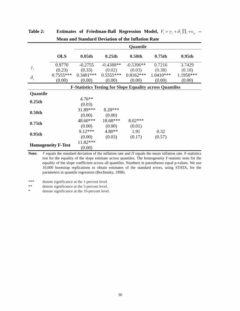
Table 2: Estimates of Friedman-Ball Regression Model, i iV v iτ τ τγ δ= + ∏ + -- Mean and Standard Deviation of the Inflation Rate

Quantile

OLS 0.05th 0.25th 0.50th 0.75th 0.95th

τγ 0.9770 (0.23)

-0.2755 (0.33)

-0.4388** (0.02)

-0.5396** (0.03)

0.7216 (0.38)

3.7429 (0.18)

τδ 0.7555*** (0.00)

0.3401*** (0.00)

0.5555*** (0.00)

0.8162*** (0.00)

1.0410*** (0.00)

1.1950*** (0.00)

F-Statistics Testing for Slope Equality across Quantiles Quantile

0.25th 4.76** (0.03)

0.50th 31.89*** (0.00)

8.28*** (0.00)

0.75th 48.60*** (0.00)

18.68*** (0.00)

8.02*** (0.01)

0.95th 9.12*** (0.00)

4.80** (0.03)

1.91 (0.17)

0.32 (0.57)

Homogeneity F-Test 11.82*** (0.00)

Note: V equals the standard deviation of the inflation rate and Π equals the mean inflation rate. F-statistics test for the equality of the slope estimate across quantiles. The homogeneity F-statistic tests for the equality of the slope coefficient across all quantiles. Numbers in parentheses equal p-values. We use 10,000 bootstrap replications to obtain estimates of the standard errors, using STATA, for the parameters in quantile regression (Buchinsky, 1998).

*** denote significance at the 1-percent level. ** denote significance at the 5-percent level. * denote significance at the 10-percent level.

30

Table 3: Estimates of Cukierman-Meltzer Regression Model, i iV u iτ τ τα βΠ = + + -- Mean and Standard Deviation of the Inflation Rate

Quantile

OLS 0.05th 0.25th 0.50th 0.75th 0.95th

τα 2.1032*** (0.00)

0.7271* (0.07)

0.8615** (0.01)

1.5311*** (0.00)

2.1072*** (0.00)

5.9568 (0.22)

τβ 0.9418*** (0.00)

0.4093*** (0.00)

0.7135*** (0.00)

0.9249*** (0.00)

1.1776*** (0.00)

1.4698*** (0.00)


0.25th 11.33*** (0.00)

0.50th 27.50*** (0.00)

5.14** (0.02)

0.75th 46.48*** (0.00)

16.75*** (0.00)

7.84*** (0.01)

0.95th 3.89*** (0.00)

1.97 (0.16)

1.06 (0.31)

0.32 (0.57)

Homogeneity F-Test 12.98***

(0.00)

Note: See Table 2. Π equals the mean inflation rate and V equals the standard deviation of the inflation rate. *** denote significance at the 1-percent level. ** denote significance at the 5-percent level. * denote significance at the 10-percent level.

31

Table 4: Estimates of Friedman-Ball Regression Model, i iV v iτ τ τγ δ= + ∏ + -- Mean and Coefficient of Variation of the Inflation Rate

Quantile

OLS 0.05th 0.25th 0.50th 0.75th 0.95th

τγ 0.9441*** (0.00)

0.2780*** (0.00)

0.3979*** (0.00)

0.6390*** (0.00)

1.2185*** (0.00)

2.1028*** (0.02)

τδ -0.0041 (0.32)

0.0008 (0.42)

0.0062** (0.03)

0.0061* (0.07)

-0.0052 (0.48)

-0.0219 (0.56)

F-Statistics Testing for Slope Equality across Quantiles Quantile 0.25th 2.22

(0.14)

0.50th 2.22

(0.24) 0.00

(0.98)

0.75th 1.21

(0.27) 5.40

(0.02) 6.23

(0.01)

0.95th 4.50**

(0.03) 7.04*** (0.01)

6.73*** (0.01)

2.67* (0.10)

Homogeneity F-Test 3.01** (0.02)

Note: See Table 2. V equals the coefficient of variation of the inflation rate and Π equals the mean inflation rate.


32

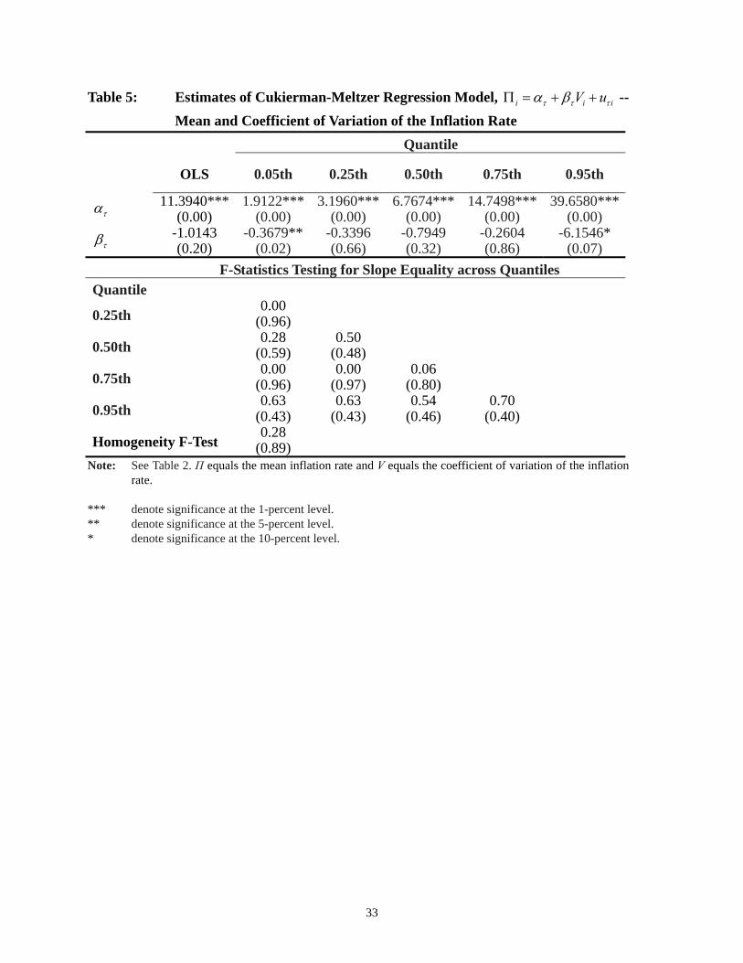
Table 5: Estimates of Cukierman-Meltzer Regression Model, i iV u iτ τ τα βΠ = + + -- Mean and Coefficient of Variation of the Inflation Rate

Quantile

OLS 0.05th 0.25th 0.50th 0.75th 0.95th

τα 11.3940*** (0.00)

1.9122***(0.00)

3.1960***(0.00)

6.7674***(0.00)

14.7498*** (0.00)

39.6580***(0.00)

τβ -1.0143 (0.20)

-0.3679** (0.02)

-0.3396 (0.66)

-0.7949 (0.32)

-0.2604 (0.86)

-6.1546* (0.07)


0.25th 0.00 (0.96)

0.50th 0.28 (0.59)

0.50 (0.48)

0.75th 0.00 (0.96)

0.00 (0.97)

0.06 (0.80)

0.95th 0.63 (0.43)

0.63 (0.43)

0.54 (0.46)

0.70 (0.40)

Homogeneity F-Test 0.28

(0.89)

Note: See Table 2. Π equals the mean inflation rate and V equals the coefficient of variation of the inflation rate.


33

Table 6: Estimates of Friedman-Ball Regression Model, i iV v iτ τ τγ δ= + ∏ + -- Median and Median Deviation of the Inflation Rate

Quantile

OLS 0.05th 0.25th 0.50th 0.75th 0.95th

τγ 3.6033*** (0.00)

-0.3312 (0.22)

-0.0152 (0.97)

0.2991 (0.51)

3.4637** (0.04)

11.5234** (0.02)

τδ 0.7617*** (0.00)

0.3567*** (0.00)

0.4765*** (0.00)

0.7417*** (0.00)

1.2889*** (0.00)

2.0668*** (0.00)

F-Statistics Testing for Slope Equality across Quantiles Quantile 0.25th 1.35

(0.25)

0.50th 5.84 (0.02)

4.05** (0.05)

0.75th 11.84*** (0.00)

10.42*** (0.00)

5.30** (0.02)

0.95th 6.70*** (0.01)

5.98** (0.02)

4.19** (0.04)

1.53 (0.22)


Note: See Table 2. V equals the median deviation of the inflation rate and Π equals the median inflation rate. *** denote significance at the 1-percent level. ** denote significance at the 5-percent level. * denote significance at the 10-percent level.

34

Table 7: Estimates of Cukierman-Meltzer Regression Model, i iV u iτ τ τα βΠ = + + -- Median and Median Deviation of the Inflation Rate

Quantile

OLS 0.05th 0.25th 0.50th 0.75th 0.95th

τα 3.1828*** (0.00)

0.7898***(0.01)

1.3728***(0.00)

2.0893***(0.00)

3.5524*** (0.00)

5.7856 (0.23)

τβ 0.4790*** (0.00)

0.0384***(0.00)

0.2528***(0.00)

0.4568***(0.00)

0.6538*** (0.00)

1.3066*** (0.00)


0.25th 13.98*** (0.00)

0.50th 19.27*** (0.00)

6.60*** (0.01)

0.75th 14.62*** (0.00)

6.83*** (0.01)

1.93 (0.17)

0.95th 7.62*** (0.01)

5.32** (0.02)

3.50* (0.06)

2.29 (0.13)


Note: See Table 2. Π equals the median inflation rate and V equals the median deviation of the inflation rate. *** denote significance at the 1-percent level. ** denote significance at the 5-percent level. * denote significance at the 10-percent level.

35

Table 8: Estimates of Friedman-Ball Regression Model with Dummy Variable, iiDiDi DDV Π+++= )( ττττ δδγγ -- Mean and Standard Deviation of the

Inflation Rate Quantile

OLS 0.05th 0.25th 0.50th 0.75th 0.95th

τγ -0.6827 (0.12)

-0.4202 (0.32)

-0.4416 (0.30)

-0.4416 (0.38)

-0.8877 (0.59)

1.0100 (0.86)

τδ 1.1149*** (0.00)

0 .4351***(0.00)

0.6317*** (0.00)

0 .8276***(0.00)

1.6226*** (0.00)

1.6663 (0.27)

Dτγ 3.0479 (0.16)

-0.4716 (0.44)

-2.0238***(0.00)

-0.7239 (0.25)

2.9819 (0.13)

5.1572 (0.50)

Dτδ -0.4101* (0.06)

-0.0860 (0.27)

0.0515 (0.66)

0.0082 (0.95)

-0.6794 (0.14)

-0.6090 (0.69)

F-Statistics 86.19*** (0.00)

17.07*** (0.00)

29.03*** (0.00)

70.65*** (0.00)

67.19*** (0.00)

39.02***(0.00)

Note: See Table 2. V equals the standard deviation of the inflation rate and Π equals the mean inflation rate. F-statistics test for the equality of the intercept and slope estimates across low- and high-inflation countries.


36

Table 9: Estimates of Friedman-Ball Regression Model, i iV v iτ τ τγ δ= + ∏ + --

Mean and Standard Deviation of the Inflation Rate Panel A: High-Inflation Countries Quantile

OLS 0.05th 0.25th 0.50th 0.75th 0.95th

τγ 2.3651 (0.12)

-0.8919 (0.18)

-2.4655* (0.06)

-1.1654 (0.55)

2.0942 (0.38)

6.1672 (0.15)

τδ 0.7048*** (0.00)

0.3491*** (0.00)

0.6832*** (0.00)

0.8358*** (0.00)

0.9432*** (0.00)

1.0573*** (0.00)


0.25th 5.05** (0.03)

0.50th 9.71*** (0.00)

1.25 (0.27)

0.75th 11.77*** (0.00)

2.44 (0.12)

0.78 (0.38)

0.95th 5.28*** (0.02)

1.41 (0.24)

0.56 (0.46)

0.15 (0.70)


Panel B: Low-Inflation Countries Quantile

OLS 0.05th 0.25th 0.50th 0.75th 0.95th τγ -0.6828

(0.20) -0.4203 (0.00)

-0.4416* (0.10)

-0.4416 (0.25)

-0.8877 (0.414)

1.0100 (0.33)

τδ 1.1149*** (0.00)

0.4351*** (0.00)

0.6317*** (0.00)

0.8276*** (0.00)

1.6226*** (0.00)

1.6663*** (0.00)


0.25th 2.65 (0.11)

0.50th 5.29** (0.02)

1.80 (0.18)

0.75th 8.92*** (0.00)

6.86*** (0.01)

5.09** (0.03)

0.95th 21.72*** (0.00)

15.02*** (0.00)

8.87*** (0.00)

0.01 (0.92)


Note: See Table 2. V equals the standard deviation of the inflation rate and Π equals the mean inflation rate. *** denote significance at the 1-percent level. ** denote significance at the 5-percent level. * denote significance at the 10-percent level.

37

Table 10: Countries that Target Inflation

Inflation Targeting

Adoption Year* Current Inflation Target (percent)

Emerging market countries

Israel 1997 1-3 Czech Republic 1998 3(+/-1) Korea 1998 2.5-3.5 Poland 1999 2.5(+/-1) Brazil 1999 4.5(+/-2.5) Chile 1999 2-4 Colombia 1999 5(+/-0.5) South Africa 2000 3-6 Thailand 2000 0-3.5 Mexico 2001 3(+/-1) Hungary 2001 3.5(+/-1) Peru 2002 2.5(+/-1) Philippines 2002 5-6 Industrial countries

New Zealand 1990 1-3 Canada 1991 1-3 United Kingdom 1992 2 Australia 1993 2-3 Sweden 1993 2(+/-1) Switzerland 2000 <2 Iceland 2001 2.5 Norway 2001 2.5 Note: IMF, World Economic Outlook, 2005. * This year indicates when countries de facto adopted inflation targeting. Official adoption dates

may vary.

38

Table 11: Estimates of Friedman-Ball Regression Model with Dummy Variable, iiDiDi DDV Π+++= )( ττττ δδγγ , for the Low-Inflation Sample -- Mean and

Standard Deviation of the Inflation Rate Quantile

OLS 0.05th 0.25th 0.50th 0.75th 0.95th

τγ 0.2334 (0.72)

0.2969** (0.04)

0.5892* (0.09)

0.8467 (0.12)

1.3292 (0.27)

0.9164 (0.71)

τδ 0.6301 (0.14)

0.1106 (0.28)

0.0740 (0.65)

0.1089 (0.68)

0.1084 (0.86)

1.8866 (0.25)

Dτγ -1.5822 (0.34)

-1.5788***(0.00)

-2.4885*** (0.00)

-1.8637* (0.07)

-6.5831*** (0.00)

-0.1599 (0.95)

Dτδ 0.6342 (0.26)

0.5823*** (0.00)

0.8544*** (0.00)

0.8706 (0.01)

2.5125 (0.00)

-0.1765 (0.92)

F-Statistics 19.48*** (0.00)

18.02*** (0.00)

11.91*** (0.00)

3.37** (0.02)

14.60*** (0.00)

20.75*** (0.00)

Obs. 76 Note: See Table 2. V equals the standard deviation of the inflation rate and Π equals the mean inflation rate.

F-statistics test for the equality of the intercept and slope estimates across low- and high-inflation countries.


39

Table 12: Estimates of Friedman-Ball Regression Model, i iV v iτ τ τγ δ= + Π + , for the

Low-Inflation Sample -- Mean and Standard Deviation of the Inflation Rate

Panel A: Moderate-Inflation Countries Quantile OLS 0.05th 0.25th 0.50th 0.75th 0.95th

τγ -1.3488 (0.37)

-1.2819***(0.00)

-1.8992* (0.07)

-1.0170 (0.77)

-5.2539** (0.02)

0.7565 (0.14)

τδ 1.2644*** (0.00)

0.6929*** (0.00)

0.9284*** (0.00)

0.9794 (0.19)

2.6209*** (0.00)

1.7101*** (0.00)

Obs. 38


0.25th 1.02 (0.32)

0.50th 0.22 (0.64)

0.01 (0.93)

0.75th 5.18** (0.03)

4.30** (0.05)

3.84* (0.06)

0.95th 2.02 (0.16)

1.21 (0.28)

0.72 (0.40)

0.97 (0.33)


Panel B: Low-Inflation Countries Quantile

OLS 0.05th 0.25th 0.50th 0.75th 0.95th

τγ 0.2334 (0.72)

0.2969*** (0.00)

0.5892*** (0.01)

0.8467* (0.07)

1.3292 (0.18)

0.9164 (0.67)

τδ 0.6301 (0.14)

0.1106*** (0.00)

0.0740 (0.46)

0.1089 (0.63)

0.1084 (0.82)

1.8866 (0.19)

Obs. 38


0.25th 0.05 (0.83)

0.50th 0.00 (0.99)

0.04 (0.84)

0.75th 0.00 (1.00)

0.01 (0.92)

0.00 (1.00)

0.95th 2.72 (0.11)

2.95* (0.09)

2.96* (0.09)

3.46* (0.07)

Homogeneity F-Test 0.78 (0.57)


40

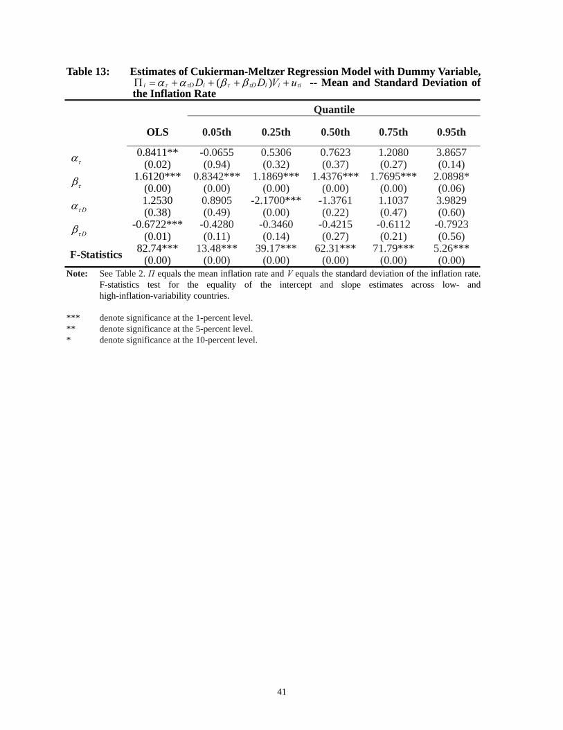
Table 13: Estimates of Cukierman-Meltzer Regression Model with Dummy Variable, iiiDiDi uVDD τττττ ββαα ++++=Π )( -- Mean and Standard Deviation of

the Inflation Rate Quantile

OLS 0.05th 0.25th 0.50th 0.75th 0.95th

τα 0.8411** (0.02)

-0.0655 (0.94)

0.5306 (0.32)

0.7623 (0.37)

1.2080 (0.27)

3.8657 (0.14)

τβ 1.6120*** (0.00)

0.8342*** (0.00)

1.1869*** (0.00)

1.4376*** (0.00)

1.7695*** (0.00)

2.0898* (0.06)

Dτα 1.2530 (0.38)

0.8905 (0.49)

-2.1700***(0.00)

-1.3761 (0.22)

1.1037 (0.47)

3.9829 (0.60)

Dτβ -0.6722*** (0.01)

-0.4280 (0.11)

-0.3460 (0.14)

-0.4215 (0.27)

-0.6112 (0.21)

-0.7923 (0.56)

F-Statistics 82.74*** (0.00)

13.48*** (0.00)

39.17*** (0.00)

62.31*** (0.00)

71.79*** (0.00)

5.26*** (0.00)

Note: See Table 2. Π equals the mean inflation rate and V equals the standard deviation of the inflation rate. F-statistics test for the equality of the intercept and slope estimates across low- and high-inflation-variability countries.


41

Table 14: Estimates of Cukierman-Meltzer Regression Model, i iV u iτ τ τα βΠ = + + -- Mean and Standard Deviation of the Inflation Rate

Panel A: High-Inflation-Variability Countries Quantile

OLS 0.05th 0.25th 0.50th 0.75th 0.95th

τα 2.0941 (0.13)

0.8250 (0.30)

-1.6393 (0.14)

-0.6138 (0.78)

2.3117 (0.34)

7.8486 (0.26)

τβ 0.9397*** (0.00)

0.4063*** (0.00)

0.8409*** (0.00)

1.0162*** (0.00)

1.1584*** (0.00)

1.2975*** (0.00)


0.25th 7.20*** (0.01)

0.50th 11.00*** (0.00)

1.85 (0.18)

0.75th 13.37*** (0.00)

3.87** (0.05)

1.10 (0.30)

0.95th 1.39 (0.24)

0.36 (0.55)

0.14 (0.71)

0.03 (0.85)


Panel B: Low-Inflation-Variability Countries Quantile

OLS 0.05th 0.25th 0.50th 0.75th 0.95th

τα 0.8411** (0.02)

-0.0655 (0.91)

0.5306 (0.15)

0.7623 (0.12)

1.2080* (0.09)

3.8657 (0.30)

τβ 1.6120*** (0.00)

0.8342*** (0.00)

1.1869*** (0.00)

1.4376*** (0.00)

1.7695*** (0.00)

2.0898*** (0.00)


0.25th 1.15 (0.29)

0.50th 2.85* (0.10)

1.29 (0.26)

0.75th 2.94* (0.09)

1.56 (0.21)

0.67 (0.42)

0.95th 1.20 (0.28)

0.65 (0.42)

0.35 (0.55)

0.08 (0.78)



42

Table 15: Estimates of Cukierman-Meltzer Regression Model with Dummy Variable iiiDiDi uVDD τττττ ββαα ++++=Π )( , for the

Low-Inflation-Variability Sample -- Mean and Standard Deviation of the Inflation Rate

Quantile

OLS 0.05th 0.25th 0.50th 0.75th 0.95th

τα 0.6712 (0.42)

1.2199 (0.11)

1.5252* (0.10)

1.0782 (0.31)

0.9979 (0.35)

0.4377 (0.85)

τβ 1.6457* (0.10)

-0.4625 (0.33)

0.0873 (0.92)

0.9991 (0.30)

2.0190** (0.04)

4.1159 (0.16)

Dτα 1.4367 (0.41)

-1.1572 (0.40)

-2.3144* (0.09)

0.7400 (0.66)

4.2652*** (0.01)

4.9459 (0.23)

Dτβ -0.4301 (0.70)

1.2668** (0.03)

1.6118* (0.08)

0.1635 (0.88)

-1.4991 (0.16)

-2.384 (0.43)

F-Statistics 27.63*** (0.00)

4.57*** (0.01)

15.51*** (0.00)

18.11*** (0.00)

9.35*** (0.00)

26.20*** (0.00)

Obs. 76 Note: See Table 2. V equals the standard deviation of the inflation rate and Π equals the mean inflation rate.

F-statistics test for the equality of the intercept and slope estimates across low- and high-inflation-variability countries.


43

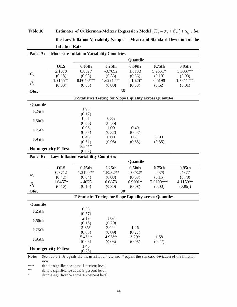
Table 16: Estimates of Cukierman-Meltzer Regression Model , i iV u iτ τ τα βΠ = + + , for

the Low-Inflation-Variability Sample -- Mean and Standard Deviation of the Inflation Rate

Panel A: Moderate-Inflation Variability Countries Quantile OLS 0.05th 0.25th 0.50th 0.75th 0.95th

τα 2.1079 (0.18)

0.0627 (0.95)

-0.7892 (0.53)

1.8183 (0.36)

5.2631* (0.10)

5.3837** (0.03)

τβ 1.2155** (0.03)

0.8043*** (0.00)

1.6991*** (0.00)

1.1626* (0.09)

0.5199 (0.62)

1.7311*** (0.01)

Obs. 38


0.25th 1.97 (0.17)

0.50th 0.21 (0.65)

0.85 (0.36)

0.75th 0.05 (0.83)

1.00 (0.32)

0.40 (0.53)

0.95th 0.43 (0.51)

0.00 (0.98)

0.21 (0.65)

0.90 (0.35)

Homogeneity F-Test 3.24** (0.02)

Panel B: Low-Inflation Variability Countries Quantile

OLS 0.05th 0.25th 0.50th 0.75th 0.95th

τα 0.6712 (0.42)

1.2199** (0.04)

1.5252** (0.03)

1.0782* (0.08)

.9979 (0.16)

.4377 (0.78)

τβ 1.6457* (0.10)

-.4625 (0.19)

0.0873 (0.89)

0.9991* (0.08)

2.0190*** (0.00)

4.1159** (0.05))

Obs. 38 F-Statistics Testing for Slope Equality across Quantiles

Quantile

0.25th 0.33 (0.57)

0.50th 2.19 (0.15)

1.67 (0.20)

0.75th 3.35* (0.08)

3.02* (0.09)

1.26 (0.27)

0.95th 5.45** (0.03)

4.93** (0.03)

3.20* (0.08)

1.58 (0.22)


Note: See Table 2. Π equals the mean inflation rate and V equals the standard deviation of the inflation rate.


44

020

4060

80

infla

tion

unce

rtani

ty

0 20 40 60inflation

Regression Lines as Quantile Varies

Figure 1: Quantile Regressions of Mean Inflation on Its Standard Deviation

(Plots of Results in Table 2)

0.5

11.

52

Slo

pe a

nd c

onfid

ence

ban

ds

0 .2 .4 .6 .8 1Quantile

Figure 2: Plot of Slope Coefficient on the Standard Deviation in Quantile Regressions (Quantiles Run from 0.05 to 0.95 in Increments of 0.05).

45

020

4060

80

infla

tion

0 10 20 30 40 50inflation uncertanity


Figure 3: Quantile Regressions of the Standard Deviation onto Mean Inflation (Plots of Results in Table 3)

0.5

11.

52

2.5

Slo

pe a

nd c

onfid

ence

ban

ds

0 .2 .4 .6 .8 1Quantile

Figure 4: Plot of Slope Coefficient in Mean Inflation Quantile Regressions (Quantiles Run from 0.05 to 0.95 in Increments of 0.05).

46

02

46

infla

tion

unce

rtain

ty

0 20 40 60 80inflation


Figure 5: Quantile Regressions of Mean Inflation on Its Coefficient of Variation


-.04

-.02

0.0

2S

lope

and

con

fiden

ce b

ands

0 .2 .4 .6 .8 1Quantile

Figure 6: Plot of Slope Coefficient on the Coefficient of Variation in Quantile Regressions

(Quantiles Run from 0.05 to 0.95 in Increments of 0.05).

47

020

4060

80

infla

tion

0 2 4 6inflation uncertanity


Figure 7: Quantile Regressions of the Coefficient of Variation onto Mean Inflation (Plots of Results in Table 5)

-20

-10

010

Slo

pe a

nd c

onfid

ence

ban

ds

0 .2 .4 .6 .8 1Quantile

Figure 8: Plot of Slope Coefficient in Mean Inflation Quantile Regressions


48

050

100

150

infla

tion

unce

rtani

ty

0 20 40 60 80inflation


Figure 9: Quantile Regressions of Median Inflation on Its Median Deviation


01

23

4S

lope

and

con

fiden

ce b

ands

0 .2 .4 .6 .8 1Quantile

Figure 10: Plot of Slope Coefficient on the Median Deviation in Quantile Regressions


49

020

4060

80in

flatio

n

0 20 40 60inflation uncertanity


Figure 11: Quantile Regressions of the Median Deviation onto Median Inflation


0.5

11.

52

Slo

pe a

nd c

onfid

ence

ban

ds

0 .2 .4 .6 .8 1Quantile

Figure 12: Plot of Slope Coefficient in Median Inflation Quantile Regressions


50

Appendix Table: Average Annual Inflation (Percent) in Sample Countries: 1993-2003 Country Π Country Π Country Π Country Π Albania 17.61 Ecuador 35.72 Latvia 10.40 Saudi Arabia (L) 0.43

Algeria 10.90 Egypt, Arab Rep. 6.09 Lesotho 9.62 Senegal 4.72

Argentina 5.08 El Salvador 6.04 Lithuania 15.26 Seychelles 2.46

Australia 2.56 Estonia 20.55 Luxembourg 2.03 Sierra Leone 16.88

Austria 1.97 Ethiopia 3.71 Macedonia 16.12 Singapore 1.16

Azerbaijan 2.89 Fiji 2.96 Madagascar 15.64 Slovak Republic 8.37

Bahamas 1.78 Finland 1.54 Malawi 30.79 Slovenia 11.81

Bahrain (L) 0.71 France 1.57 Malaysia 2.79 Solomon Islands 9.67

Bangladesh 4.91 Gabon 6.37 Maldives 3.81 South Africa 7.40

Barbados 1.84 Gambia, The 3.79 Mali 4.89 Spain 3.34

Belgium 1.87 Georgia 11.93 Malta 2.76 Sri Lanka 9.42

Belize 1.72 Germany 1.78 Mauritania 5.32 St. Kitts and Nevis 2.95

Benin 7.27 Ghana 28.21 Mauritius 6.44 St. Lucia 2.11

Bhutan 6.53 Greece 6.28 Mexico 14.97 St. Vincent 1.56

Bolivia 5.82 Grenada 1.86 Moldova 16.85 Sudan (H) 50.99

Botswana 9.18 Guatemala 8.21 Mongolia 26.86 Suriname 32.61

Brazil 14.87 Guinea-Bissau 20.42 Morocco 2.76 Swaziland 9.39

Bulgaria 39.95 Guyana 6.14 Mozambique 24.73 Sweden 1.65

Burkina Faso 4.95 Haiti 21.28 Namibia 8.91 Switzerland (L) 1.08

Burundi 14.63 Honduras 15.22 Nepal 6.30 Syrian Arab Rep. 4.23

Cambodia 4.02 Hong Kong 2.43 Netherlands 2.59 Tanzania 14.55

Cameroon 5.96 Hungary 14.97 New Zealand 1.99 Thailand 3.61

Canada 1.85 Iceland 3.19 Nicaragua 10.11 Togo 6.94

Cape Verde 4.37 India 6.98 Niger 5.80 Tonga 4.81

Central African Rep. 5.09 Indonesia 14.04 Nigeria 26.73 Trinidad and Tobago 5.27

Chad 7.76 Iran, Islamic Rep. 22.10 Norway 2.22 Tunisia 3.50

Chile 6.10 Ireland 2.92 Pakistan 7.32 Turkey (H) 68.69

China 5.97 Israel 6.62 Panama (L) 1.03 Uganda 5.20

Colombia 15.12 Italy 3.08 Papua New Guinea 10.96 Ukraine 21.96

Congo, Rep. 8.33 Jamaica 14.57 Paraguay 11.66 United Kingdom 2.48

Costa Rica 12.71 Japan (L) 0.13 Peru 11.13 United States 2.49

Cote d'Ivoire 6.16 Jordan 2.64 Philippines 6.45 Uruguay 22.56

Croatia 14.15 Kazakhstan 13.23 Poland 15.49 Vanuatu 2.56

Cyprus 3.24 Kenya 12.41 Portugal 3.66 Venezuela (H) 40.94

Czech Republic 5.97 Korea 4.16 Romania (H) 58.54 Vietnam 3.13

Denmark 2.16 Kuwait 1.71 Russian Federation 30.95 Yemen, Rep. 20.67

Dominica 1.21 Kyrgyz Rep. 16.62 Rwanda 5.81 Zambia 30.88

Dominican Republic 9.12 Lao PDR 31.96 Samoa 3.51 Zimbabwe (H) 47.56

Note: L and H mean the 5 lowest and 5 highest inflation rates.

51

Does a Threshold Inflation Rate Exist?

Documents

Transcript of Does a Threshold Inflation Rate Exist?