Threshold models of collective behavior - IFISC

d= bounded confidence or opinion uncertainty

Deffuant et al, Adv. Comp. Syst. 3, 87 (2000)

Bounded confidence model

< d

Infection, contagion and spreading

How and when a disease, rumor, idea… propagates from a seed and fills the whole system

Models of simple contagion: SIS: Susceptible-Infected-Susceptible SIR: Susceptible-Infected Recovered/Removed

S I S λ β

S I R λ β

Typically the SIS model in a network displays a phase transition for a critical value of the propagation rate λc. Random networks

2k

kc

Scale Free Networks

Eguíluz, Klemm, PRL 89, 108701 (2002)

http://rocs.hu-berlin.de/explorables/explorables/sirs/

http://rocs.hu-berlin.de/explorables/explorables/epidemonic/

M. Granovetter The American J. Sociol. 83 (1978)

Simple vs Complex Contagion:

Can contagion be transmitted by a single “infected” node? Innovations, rumors, riots, fashions…. One neighbor acting alone is RARELY sufficient to trigger a cascade of activation: node activation requires simultaneous exposure to multiple active neighbors

Set of N elements located at the nodes of a network with states: si = ±1

Each node is assigned a threshold 0 ≤ T ≤ 1, which determines the number of neighbors required for node i to change her state.

Initial condition: a fraction p of nodes with state (-1)

THRESHOLD DYNAMICS:

An agent i with state si =+1 is randomly chosen in the network (called active node) . If the number of neighbors of agent i in a state -1 is larger than the threshold "T", then the active agent changes its state to si =-1 Otherwise it remains as si =+1

Granovetter´s Threshold Model: Complex Contagion

D. Centola et al. Physica A 374,449 (2007) D. Centola, Science 329, 1194 (2010)

Threshold models of collective behavior


The models of this paper treat binary decisions those where an actor has two distinct and mutually exclusive behavioral alternatives. In most cases the decision can be thought of as having a positive and negative side-deciding to do a thing or not to, as in deciding whether to join a riot-though this is not required for the formal analysis. A further requirement is that the decision be one where the costs and benefits to the actor of making one or the other choice depend in part on how many others make which choice. We may take riots as an example. The cost to an individual of joining a riot declines as riot size increases, since the probability of being apprehended is smaller the larger the number involved (see, e.g., Berk 1974). The individuals in these models are assumed rational that is, given their goals and preferences, and their perception of their situations, they act so as to maximize their utility. The crucial concept for describing such variation among individuals is that of "threshold." A person's threshold for joining a riot is defined here as the proportion of the group he would have to see join before he would do so. A "radical" will have a low threshold: the benefits of rioting are high to him, the cost of arrest, low. Some would be sufficiently radical to have a threshold of 0%-people who will riot even when no one else does. These are the "instigators Conservatives will have high thresholds: the benefits of rioting are small or negative to them and the consequences of arrest high since they are likely to be "respectable citizens" rather than "known rabble-rousers." Thresholds of 80% or 90%0 may be common, and we may allow for those individuals who would not join under any circumstances by assigning them a threshold of 100%.


It is not necessary, in fact, to be able to classify a person as radical or conservative from his threshold, and one strength of the concept is that it permits us to avoid such crude dichotomies. Since a threshold is the result of some (possibly complex) combination of costs and benefits, two individuals whose thresholds are the same may not be politically identical, as reflected in the popular expression, "strange bedfellows." The threshold is simply that point where the perceived benefits to an individual of doing the thing in question (here, joining the riot) exceed the perceived costs.

… Suggested applications are to riot behavior, Innovation and rumor diffusion, voting and migration

I have adapted the idea of behavioral thresholds from Schelling's models of residential segregation (1971a, 1971b, 1972), where thresholds are for leaving one's neighborhood, as a function of how many of one's own color also do so. The present paper has Schelling's aim of predicting equilibrium outcomes from distributions of thresholds but generalizes some features of the analysis and carries it in somewhat different directions




D.J. Watts, PNAS 99, 5766 (2002)

Consider a random graph of size N in which all the nodes have the same degree <k> << N and the same threshold T.

Let i be the focal node of a seed neighborhood with <k> active neighbors. For large enough N, there will be a node j connected to an active neighbor of i:

Simple propagation is therefore assured, as it only requires one active neighbor for a node to be activated.

However, multiple propagation requires that there be, at the very least, a second node active that is adjacent to j. As N approaches infinity in a sparse network, the probability that j has a second neighbor among the seed neighborhood approaches zero. Thus, the critical threshold for a random graph is approximated by

kT r

c

1


local

How and when a disease, rumor, innovation… propagates from a SEED and fills the whole system? Simple vs. Complex contagion

COMPLEX SIMPLE

M. Granovetter The American J. Sociol. 83 (1978) D.J. Watts, PNAS 99, 5766 (2002)

Simple vs Complex contagions

Centola, D.; Eguíluz, V. M.; Macy, M.W. Physica A 374, 449-456 (2007)

Simple vs Complex contagions

Simple Contagion Complex Contagion

Interaction Pairwise (dyadic) interactions Collective interactions

Rule Single exposure Multiple exposures

Phase

transition Second order transitions First order transitions

Examples Epidemic spreading

(SIR, SIS, etc)

Social contagion

(Threshold model etc)

T=1/2 Spin Flip Kinetic Ising Model at 0ºK

Set of N elements located at the nodes of a network with states: si = ±1

Each node is assigned a threshold 0 ≤ T ≤ 1, which determines the number of neighbors required for node i to change her state.

Initial condition: a fraction p of nodes with state (+1) uniformly distributed (p= 50% often)

THRESHOLD DYNAMICS:

An agent i with state si is randomly chosen in the network

If the number of neighbors of agent i in a state different from si is larger than the threshold "T", then agent changes i its state to -si . Otherwise it remains with si

In the case that the fraction of neighbors in a different state is equal to the threshold "T", then with probability 1/2, the active agent changes its state


Consensus vs Infection: Symmetric Granovetter´s Threshold Model


K = 4

K = 8

Phase diagram (+o,T)

I II

II

III

+o

= initial density of nodes with state 1

+f = final density of nodes with state -1

Phase I : Disorder (active) (T<Tc= 3/8, K=8) Phase II : Order (T=3/8,4/8,5/8) Phase III : Disorder (Frozen) (T>Tc*=5/8, K=8)

K=8

Symmetric Threshold Model

Regular lattice


Visualization regular network K=8

I: Disordered active state: T=1,2. Final state independent of initial condition

Minority spreading to 50%: T=2 (i= 0.08, 0.13)

II: Ordered state, T=3,4. Final state depends on initial condition i= 0.2, 0.8

III: Disordered state, T=5,6,7,8. Final state depends on initial condition

local

Persistence p(t) (fraction of nodes that persist in the same state as t=0 up to some later time t)

N = 104

+o=0.5

q 0.22

k = 4

k = 8

T = 1/8,2/8

T = 3/8,4/8 T > 4/8

qttp ~)(

qttp ~)(

I: T<Tc, p(t) ~ a exp (-b ln2 t)

II: Tc<T<Tc*, p(t) ~ t q

III: T>Tc*, p(t) ~ constant



Phase I : Disorder (active) Phase II : Order Phase III : Disorder (Frozen)

+o

= initial density of nodes with state 1

+f = final density of nodes with state -1

I II

III

II

Random Network


Symmetric Granovetter´s Model with distributed thresholds Set of N elements located at the nodes of a network Each nodes can take two possible states: s

i = ±1 (opinion, action)

Initial condition: a fraction p of nodes with state (+1) are uniformly distributed and 1-p with state (-1)

The system evolves by iterating the following time steps: • A agent i is randomly chosen in the network (called active node) • The threshold value of the active node is assigned at random. This threshold follows a Gaussian distribution with T as mean value and S as standard deviation:

The threshold value for each agent changes in each iteration (Same than original Granovetter)

• If the number of neighbors of agent i in a state different that si is larger than the threshold "T", then the active agent

changes its state (si) to (-s

i). Otherwise it keeps the state

In the case that the fraction of neighbors in a different state is equal to the threshold "T", then with probability 1/2, the active agent changes its state


HETEROGENEOUS AGENTS

Phase diagram (+o,T) Phase diagram (+

o,T)


S =0 S =0.01

S =0.10

Regular lattice, N=106

Heterogeneity destroys frozen disordered state III

T=6, i=0.6, S=0-0.1


local

I

II

II

III




N = 106

S =0 S =0.01

S =0.1


Fully Connected Network

Social learning: Information aggregation

Two ingredients: Competition between local and external interactions:

Local: Each element interacts with others typically in a range << system size

(interaction with nearest neighbors)

External: Each element experiences the influence of a common environment acting on the entire system (e.g. mean field, external signal).

Consumers choosing a product: opinion people they trust + information gathered from prices, advertisement.

Voters, citizens: climate change/global warming, nuclear plants, European treaty, national debt, E. coli. Individuals confront external signals to the information gathered from their contacts,

Social learning

Social learning; is the ability of a population to aggregate information.

It depends on: the information mechanism by which agents learn from each other, and therefore on the underlying social network in which they are embedded.

Noisy external signal: flow of fresh information generated independent of agent’s position (health consequences of consuming a particular good, severity of climate change).

Confronted with the behavior displayed by the neighbors.

Social learning

Model: Each agent can choose between two states, Si = +1 or Si=-1. and characterized by a threshold ti Dynamical rules: 1 Agent i is randomly chosen and receives an external signal E, with p E=+1 and (1-p) E=-1

2 if E = Si nothing happens. if E ≠ Si then if the fraction of neighbors with opposite state is greater than ti, then Si -Si

Initial condition: fraction p in state +1, and 1-p in state -1

Question: What is the relationship between p (the quality of the signal) and t (the threshold for state change) that underlies the spread and consolidation of state 1?

Social learning All agents in a system adopt (“learn”) the state of an external signal as a consequence of their

local interactions and the interaction with that signal.

González-Avella, et al. PLoS ONE 6(5), e20207

t+1

E E

t

x(t) = fraction of agents choosing action 1 at time t

Social learning: global interaction

)()1()1()1( tqtq xxpxxpx

where q(z) = 1 if z ≥ 0; while q(z) = 0 if z < 0. It is useful to divide the analysis into two cases:


20t

60.0p

6.0

6.0

5.0

t

t

t

p

p

case

4.0

6.0

1

5.0

t

t

t

p

p

case

p 1t

pt

II

III

I

I II III

Phase I: Disorder (active) Phase II: Order Phase III: Disorder (Frozen)

Phase I for t <0.5

Phase III for t >0.5

Phase diagram (p,t) N=104

50.0t20.0t 80.0t

Social learning: global interaction


PHASE II

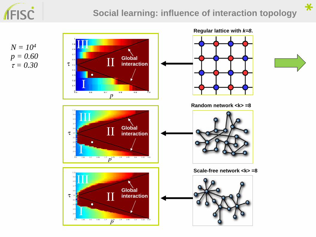
N = 104

p = 0.60 t = 0.30

II

I

I

II

III

II

I

Regular lattice with k=8.

Random network <k> =8

Scale-free network <k> =8

Social learning: influence of interaction topology

Global interaction

Global interaction

Global interaction

III

III

II Global interaction

Global interaction


Threshold models of collective behavior - IFISC

Documents

Transcript of Threshold models of collective behavior - IFISC