DESCRIBING THE RHEOLOGY OF VIBRATED, NO-SLUMP CONCRETE FORAPPLICATION IN 3D-PRINTING CONSTRUCTION

BY

KATHLEEN ADELLE HAWKINS

THESIS

Submitted in partial fulfillment of the requirementsfor the degree of Master of Science in Civil and Environmental Engineering

in the Graduate College of theUniversity of Illinois at Urbana-Champaign, 2018

Urbana, Illinois

Adviser:

Professor David Lange

ii

ABSTRACT

Using an automated process like 3D printing in concrete construction could improve safety and

performance while decreasing environmental impact and cost. But 3D-printed concrete

construction still needs considerable development before it will be reliable. This research

addresses the challenge of extruding concrete, which must be fluid enough to flow through an

extruding nozzle but solid enough to retain its shape when placed in layers. It focuses on

controlling the fluid/solid state of the concrete with vibration. In rheological literature, vibration

has been shown to overcome the yield stress of granular suspensions, permitting them to behave

as solids at low strain rates. Most models describe two regimes, one describing Newtonian

behavior at low strain rates and the second describing a return to the original, non-vibrated

behavior at higher strain rates. Concrete can be considered a volume of aggregates suspended in

cement paste and therefore a granular suspension. Several constitutive models have been

proposed to describe the rheological behavior of vibrated granular suspensions but only on

idealized fluids and at small scales. This study investigated how well these models apply to

granular suspensions using concrete constituents. The first series of tests were conducted on

standard concrete mixtures without vibration. Stress growth tests and flow curve tests using an

ICAR (International Center for Aggregate Research) rheometer and the slump test was

conducted on each mixture. The ICAR rheometer was not capable of characterizing no- and

low-slump concrete mixtures. It was found that the yield stress of concrete relies on the granular

phase while the viscosity relies on the cement paste phase. Because of this, the aggregate stock

must be controlled more carefully than is currently done in practice. The second series of tests

were conducted on no-slump concrete mixtures made of a bleed-resistance cement paste and

coarse limestone aggregates. The gradation was controlled so that the sizes and volume fractions

of the aggregates were known. Stress growth tests and flow curve tests were conducted using the

ICAR rheometer while the concrete was being vibrated. Accelerometers were used to measure

the acceleration profile of the concrete in the ICAR bucket. The validity of the raw data had to

be checked because the rheometer struggled to achieve steady-state conditions but enough data

points from the flow curve tests were acceptable. The data fit well to a power-law model. The

shear moduli and frequency parameter of the mixtures were characterized because they are

required in the Hanotin constitutive model but the remaining two parameters, the critical strain

and -parameter, could not be obtained from the experimental data. The shear moduli were

iii

derived from the stress growth tests. The frequency parameter was assumed to be the vibrational

strain rate experienced by the concrete and calculated from the acceleration profile measured by

the accelerometers. The agreement between the data and a power-law model and the fact that

this vibrational strain rate was at least two orders of magnitude less than the strain rates applied

during shear testing with the ICAR rheometer supported the presence of a third, intermediary

regime between the expected Newtonian and Bingham regimes with a significant range of strain

rates. Further experiments are required in order to validate the assumptions used in analysis and

investigate the extent of this intermediary regime. In the end, fully characterizing this vibration-

dependent behavior and determining a reasonable constitutive model will permit the constraints

on 3D-printing to be better understood and the new construction method to be more reliable.

iv

ACKNOWLEDGMENTS

When I started studying civil engineering in undergrad, I never expected to go to graduate

school, much less fall into the construction materials discipline. But I have unexpectedly found a

topic that I love and a career path that I know I will find delight in for a very long time.

I owe my thanks to the professors who inspired me to take this path: Prof. David Lange, whose

enthusiasm for concrete is contagious and whose advice and support has been invaluable in this

project; Prof. Jeffrey Roesler, who first introduced me to materials research and student-led

projects when I was just a sophomore; Prof. Paramita Mondal, who first introduced concrete

materials to me; and Prof. John Popovics, whose high standards have helped me become a better

writer and researcher. I especially would not be here without the support of Prof. Lange and

Prof. Roesler.

I also need to thank Jamar Brown and Tim Prunkard for their support and patience in the lab.

This research could not have been completed without their help and good humor.

When I decided to study concrete, I definitely did not expect to enter the world of concrete

rheology. My entire foundation of rheology knowledge comes from the class taught by Prof.

Randy Ewoldt, whom I owe a big thank you for doing such a good job. I would not have been

able to understand all the literature and conduct these analyses without that class.

Special thanks go to Karthik Pattaje Sooryanarayana and Lillian Lau for all their help running

experiments in the lab. Most of the experiments required at least two people and I truly

appreciate their dedicated work ethics, the fun conversations we had in lab while waiting for

concrete to set, and their strong muscles.

And finally, I want to thank my friends here in Champaign and family back in Maryland for their

advice and support throughout these two amazing years. They gave me a push forward when I

needed it, pulled me back when I was speeding or overextending myself, provided delicious food

when times were tough, and listened when I needed to talk.

v

TABLE OF CONTENTS

CHAPTER 1: PROJECT INTRODUCTION .............................................................................1CHAPTER 2: BACKGROUND ON FRESH CONCRETE RHEOLOGY ............................12CHAPTER 3: CHALLENGES OF CHARACTERIZING CONCRETE RHEOLOGY .....28

CHAPTER 4: RHEOLOGY OF VIBRATED CONCRETE...................................................34CHAPTER 5: FUTURE WORK AND CONCLUSIONS ........................................................56

REFERENCES.............................................................................................................................66APPENDIX A: UNCONFINED COMPRESSION TESTS .....................................................71

APPENDIX B: TIME-DOMAIN DATA FROM ACCELEROMETERS..............................75APPENDIX C: MATLABTM CODES ........................................................................................79

APPENDIX D: THE PECLET NUMBER ................................................................................86APPENDIX E: STRESS GROWTH TEST DATA FOR NON-VIBRATED, NO-SLUMP

CONCRETES...............................................................................................................................91

1

CHAPTER 1: PROJECT INTRODUCTION

Sustainability is a major driving force behind research. The objective of this chapter is to

explain how concrete and the infant 3D-printed concrete construction method fits into the

development of a more sustainable society. It includes an overview of the history of 3D-printed

concrete construction, a brief discussion of its advantages and disadvantages, and an introduction

to the fluid/solid paradox, one of the many challenges with 3D printing and the one that this

research specifically targets.

1.1 Research Motivation

Concrete is one of the most widely-used materials in the world. The U.S. consumed 96.8 million

tons of cement, concrete’s costliest constituent, in 2017 alone1. This is roughly equivalent to 0.3

metric tons per capita. Concrete is popular for three key reasons. First, it is cheap. The raw

material costs anywhere between $0.044 and $0.066 per kilogram2. In comparison, structural

steel, which is concrete’s biggest competitor, costs about $0.882 per kilogram3. Second,

concrete is a versatile material. With the correct formwork, it can be cast into almost any shape.

Artists and architects alike take advantage of this property to make sculptures like Christ the

Redeemer and structures like the Sydney Opera House. Many designers prefer concrete because

it is capable of producing ‘organic’ shapes more easily than steel. Concrete members are also

incredibly stiff whereas steel members must often be overdesigned to meet maximum deflection

requirements. Finally, concrete is a relatively environmentally-friendly material. It requires 1.15

MJ of energy and produces 0.09 to 0.12 kg of CO2 for every kilogram made4. Steel requires 26.5

MJ of energy and produces 1.7 to 1.9 kg of CO2 for every kilogram made4.

This does not mean that concrete is the perfect material. To the contrary, steel has a much higher

strength-to-weight ratio, making it work more efficiently than concrete. Designers have also

begun to appreciate the openness of steel frames from an architectural viewpoint. Concrete is

responsible for 6% of global greenhouse gas emissions and while the Romans were able to make

concrete structures that lasted for thousands of years, such as the Pantheon, modern concrete can

crumble after only a few decades due to susceptibility to environmental conditions.

In recent decades, new types of concrete have been developed to address these concerns and

even further optimize concrete’s economy, serviceability, and environmental footprint. Two

2

examples are self-consolidating concrete (SCC) and 3D-printable concrete. SCC addresses

serviceability and durability issues. Concrete in the field must often be vibrated to ensure that

there are no large air voids left when pouring the fresh material. SCC is so fluid that it flows

under its own self-weight and does not need any encouragement from vibration to fill the desired

space. Unfortunately, this enhanced ‘workability,’ a technical term referring to the ease with

which the fresh concrete can be placed, makes SCC prone to segregation. Segregation occurs

when the concrete’s constituents separate themselves by density. The largest aggregates flow the

shortest distance, the smallest flow the farthest distance, and the cement paste can even flow

beyond the aggregates. This creates a heterogeneous hardened material which is undesirable.

There is still room for improvement and this is one reason why the study of how concrete flows,

or concrete rheology, is important.

3D-printed concrete is a more recent development than SCC and departs from conventional

concrete practices more radically. While concrete is typically poured into place, 3D-printed

concrete is extruded or injected into two-dimensional layers that are stacked on top of each other.

This construction method is capable of decreasing the economic and environmental costs and

improving the serviceability of concrete all at once. In addition, the idea of being able to 3D

print anything, from plastic desk decorations to metal novelties and complex fiber composites to

concrete houses, has captured the public’s interest, providing necessary public support.

Companies like Total Kustom, Emerging Objects, and XtreeE have printed full-sized structures,

unique structural members, and pre-made modules for assembly. Companies have reported

decreased costs, decreased construction time, less waste materials, and more artistic flexibility5,6.

But for 3D-printed concrete to be successful, it has to meet unusually stringent and paradoxical

performance requirements during placement. The fresh mixture must be a stiff solid to ensure it

does not collapse on itself. At the same time, the mix must be fluid enough to be extruded and

placed. As a result the rheology of this concrete needs to be monitored and controlled closely.

Vibration is traditionally used to improve concrete workability. It then stands to reason that

vibration may be one of the keys to controlling the fluidity of 3D-printed concrete. Literature on

concrete’s rheological response to vibration is very limited. This study adds to the literature on

the rheology of vibrated concrete and discusses how vibration can help 3D-printed concrete be

successful.

3

1.2 3D-Printed Concrete

Since 2012, there has been incredible growth in industry and academia regarding 3D-printed

concrete research and application. The following subsections do not cover every single project

and paper, and would quickly become out-of-date even if they did. Only the projects and groups

that had a large impact on the method are referenced.

1.2.1 A Historical Overview

Dr. Behrokh Khoshnevis, a Dean’s Professor of Industrial and Systems Engineering, Civil and

Environmental Engineering, and several other engineering departments at the University of

Southern California as well as the founder of the 3D-printing company Contour Crafting,

published the first paper on contour crafting in 19987. Contour crafting is a type of 3D printing

that falls under the ‘Fused Deposition Modeling’ (FDM) category. FDM is the most common

type of 3D printing. A thin filament is extruded through a nozzle, which is attached to a printer

or extruder head, and is deposited onto a platform. The head travels in the 2D plane parallel to

the surface, leaving behind a 2D pattern. When the pattern is complete, the head moves up or the

platform moves down so that the head may now extrude a new 2D pattern directly on top of the

previous one. By continuing this process, the patterns, called ‘layers’, are vertically stacked and

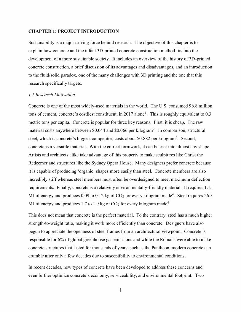
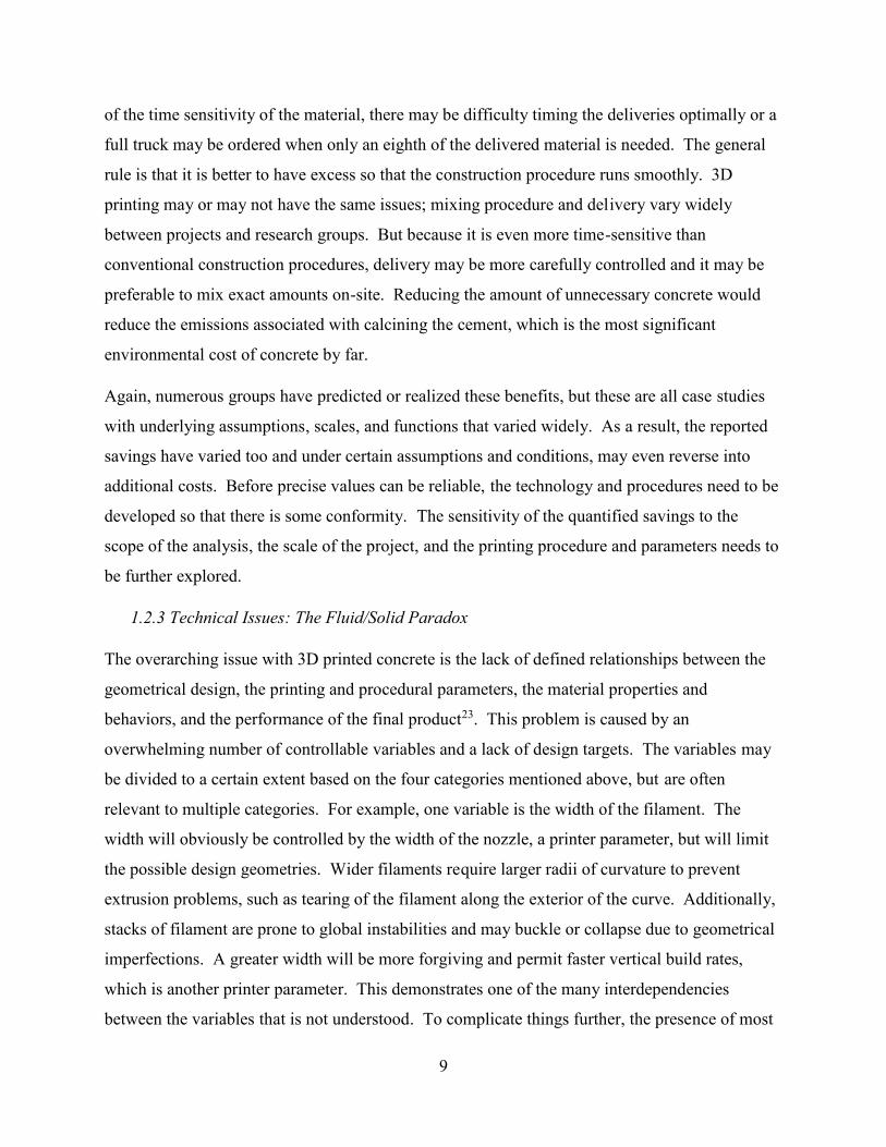
form a 3D object. A labelled image of a 3D printer using the FDM technique is shown in Figure

1 below. The printer is using two different plastic filaments, although one filament is more

common and ceramics, metals, foams, and many other materials may be 3D printed using FDM.

Koshnevis proposed that trowels traveling behind the head be used to provide a smooth finish

and make the layers indistinguishable from each other, at least externally7.

A team at Loughborough University was the second major pioneer in 3D-printed concrete. Their

first publication in 2007 focused on the potential benefits and concerns regarding this new

construction method, although later publications in 2011 and 2012 from the team focus on

developing the technology as Khoshnevis has. The 2007 publication provides a relatively unique

perspective. Many researchers and industrialists claim that 3D printing concrete can be cheaper

by using resources more efficiently and reducing waste. However, the Loughborough team’s

hypothetical studies showed that the material cost would prevent better economy and that the

construction time would not decrease8. Despite this, they argued that 3D printing concrete is

4

highly desirable because of its ability to customize and locally control material properties,

providing better functionality.

Figure 1: An example of a 3D printer printing a blown-up model of foamed cement using plasticand the FDM method (PC: Kathleen Adelle Hawkins).

Enrico Dini made the next big leap in 3D-printed concrete with a method he invented called D-

Shape. He patented the technology in 2006, founded the company Monolite UK, Ltd, and

completed his first projects in 20089,10. This method is unique because it uses particle bed

printing technology rather than FDM. The vertical stack procedure is the same, but the manner

in which the 2D patterns are made is very different. A layer of sand particles is placed and a

binder is selectively injected into the layer in the location of the desired pattern. Then a second

layer of particles is placed and the procedure is repeated. Once complete, the sand particles that

did not receive any binder are brushed away, leaving behind the completed structure. To date,

very few groups use this technology to 3D print structures.

Rael San Fratello Architects, the members of which would later become the founders of the 3D-

printing company Emerging Objects, made a significant contribution in 2009. They invented the

‘planter brick’, a ceramic brick made of crushed stones and recycled materials with sizes

Extruder headand nozzle

Platform

Printedfilament(yellow)

Printedsupportingmaterial(black)

5

between 0.2 mm and 5 mm11. These particles were held together with a variety of binders, some

of which were cementitious. This was the first instance where 3D printing was used to create a

large number of small building elements that were designed to be assembled on site. This is far

removed from the FDM process but it is worth mentioning because of the materials that were

used and because it is a reminder that extruding concrete with a massive 3D printer on-site is not

the only way to take advantage of 3D printing in construction. Many groups have developed

other ways to 3D print buildings, or structures of the same scale. Because the focus of this paper

is extruding concrete they are not included here, but Langenberg has created an infographic that

has an almost, if not fully, exhaustive list up through 20149.

The Chinese company WinSun, also called Yingchuang Building Technique (Shanghai) Co.

Ltd., made a landmark contribution when it printed ten houses in one day in 2013. The walls

were printed at its factory using a mixture of cement, sand, fiber, and a proprietary additive and

then assembled on site12. Their work has catapulted 3D-printed construction into the spotlight.

Also in 2013, Michael Hansmeyer of Computational Architecture and Benjamin Dillenburger of

Numerical Material 3D printed a structure called Digital grotesque. The material was a synthetic

sandstone and the structure has a purely artistic purpose13. Like the planter brick project, it does

not have any impact on this project, but it highlights the intense interest that architects have in

3D-printed construction, especially in Europe. To further demonstrate this, the Institute of

Advanced Architecture in Catalonia (IAAC) has made some of the most advanced developments

in 3D-printed construction. Their oldest project is the Minibuilders project, which uses three

separate robots to overcome issues of scale14. In FDM, the volume that the object is being

printed in is often bounded by a box-like gantry system. If a gantry system is used at

construction scale, then this means the gantry has to be at least as big as the structure and indeed,

most companies have tried to scale up their gantry systems9,15,6. They are much easier to control

than a swarm of robots, but would be difficult to transport from site to site. Started in 2014, the

Minibuilders project has been successful and while the robots use fast-setting artificial marble

instead of concrete14, their ability to tackle large structures makes the project relevant.

The U.S. Army Corps of Engineers (USACE) has also invested in 3D-printed concrete

construction. They started a program called “Automated Construction of Expeditionary

Structures” and their primary goal is to use 3D-printing to make semi-permanent structures with

6

local materials at any location. As a result of this program, the Construction Engineering

Research Laboratory (CERL) in Champaign, Illinois successfully 3D printed a barracks hut,

otherwise known as the B-hut, in the summer of 201716. This project is unique because their

concrete used 3/8-inch pea gravel, a large coarse aggregate, whereas most teams use cement

paste and only fine aggregates in order to achieve acceptable flow during extrusion. The

USACE also developed and patented a concrete mixture in 2018 that is 3D-printable and meets

structural strength requirements. Surprisingly, this mixture has no coarse aggregate in it and is

comprised of sand, clay, fly ash, silica fume, a binding agent, and several chemical admixtures17.

Their emphasis on the structural application is an important step in 3D-printed concrete. While

other groups such as D-Shape provide specifications describing the strength of their materials,

few have considered both structural requirements and material requirements holistically.

Other significant industry contributors include:

Total Kustom, which was founded by Andrey Rudenko and debuted in 2014 with a 3D-

printed cement paste castle6,

the WASP (World’s Advanced Saving Project) Project, which made the first reinforced

concrete beam with their printer BigDeltaWASP in 2015 and started printing a house in

201615,

XtreeE, a French company that printed a sinusoidal wall in June of 2015 and completed

its first structural project in 201718,

Apis Cor, a San Francisco-based company with a printer that uses radial instead of

Cartesian coordinates that printed a no-assembly, on-site house in 201719,

CyBe, which was founded in 2013 but delivered its first project, the R&Drone

Laboratory, in May of 2017 in Duba120, and

BetAbram, a company that develops 3D printers that use mortar as the filament and

started printing a house in 201821.

All of these teams have helped develop equipment and demonstrate the viability of 3D-printing

concrete, or at least cement paste and mortar; only CERL has used filaments that include coarse

aggregates and therefore true concrete. It is clear that 3D-printed concrete boomed in industry

starting in 2013. XtreeE, CyBe, WinSun, CERL, and IAAC appear to be the most active

currently. Neither D-Shape nor Total Kustom have announced any projects since 201510,6 and

7

the WASP Project has not completed any impactful projects with regards to 3D printing concrete

since 201615. We may see more work from them in the future though.

The Eindhoven University of Technology (TU/e) plays a unique role in the development of 3D-

printed concrete. They have been heavily involved both in the more demonstrative industrial

side and the academic side. Their 3D concrete printing project (3DCP) started in 2015 when

they began participating in relevant symposiums and conferences. Their team began publishing

papers in 2016 and have worked on several to-scale projects in 201722. Their project uses a

gantry system and FDM, and their work has been particularly impressive because it has included

structural analyses of 3D-printed concrete, an important safety concern that none of the other

projects discuss. The USACE is the only other team that has openly considered the structural

requirements of 3D-printed concrete and their work has focused more on the material properties

than the

3D-printed concrete boomed in the academic world a few years later than in the industrial one;

the number of publications spiked abruptly in 2016 and has continued to grow since. As Bos et.

al. stated, every review of current work becomes out-of-date almost immediately23. However,

Buswell et. al. published an excellent overview in May 2018 of the current state of 3D-printed

concrete research and all the questions and concerns that need to be addressed24.

1.2.2 Benefits and Drawbacks

As mentioned previously, literature states that 3D-printed concrete construction could be

beneficial environmentally, economically, and functionally. These are the three pillars of

sustainability and practices almost never excel in all three because there are trade-offs between

them. For example, products of higher quality often cost more or as another example, many

products that are economically competitive create more waste than their more expensive

counterparts. If 3D-printed concrete truly does improve all three areas, and then overall

sustainability, then it could be one of the most impactful developments of our time.

Unfortunately, 3D-printed concrete construction is still so early in its infancy that it is difficult to

say if it truly represents a more sustainable path. There is general agreement that once fully

developed, it will be able to address current issues in construction industry and improve

serviceability. The use of a relatively small filament rather than a large batch of fresh concrete,

8

as is used in conventional practice, means that different types of concrete can be placed locally in

3D printing8. The material can be tailored to meet requirements on a very local level, improving

the performance efficiency and reducing trade-off concerns in mixture design. This is one of the

primary goals of the 3DCP project at Eindhoven University of Technology23. Unfortunately, this

may cause a trade-off with cost8. In order to be localized, the layer heights need to be very small

but layer height is one of the biggest factors to control print time. Smaller layer heights result in

longer print times, which would increase economic and environmental costs. A second safety

benefit of introducing automation to the construction industry is the reduction in health and

safety risks taken by construction workers8,23. 3D-printed concrete construction requires fewer

people and possibly less time and has been proposed for use in hostile environments such as

space.

This improvement in safety and performance provides a compelling argument for the

development of 3D-printed concrete even if it does not decrease environmental and economic

costs. But because sustainability is highly desirable, researchers are working hard to develop

3D-printed concrete construction methods that have environmental and economic benefits. Cost

is expected to decrease because of the elimination of formwork, which accounts for 40% to 50%

of the construction cost, and the decreased need for skilled labor23,25. Many hypothetical

analyses predicted, and printed projects demonstrated, that the construction time truly will

decrease at the layer heights used currently6,12,15,, which are typically a few centimeters in scale.

This scale would be fully capable of local customization and so the 2007 study by the

Loughborough University team appears inaccurate. The decreased construction time would be a

third major contributor to the decrease in cost.

The primary argument for the environmental benefits of 3D-printed concrete is the decreased

waste material19,24, whether it is one-use formwork or extra concrete. Formwork must often be

specialized for the designed geometry of the construction project and is disposed of because it

cannot be used for other projects. The elimination of formwork eliminates the consumption of

wood, the gaseous emissions from extraction and manufacture, and the consumption of

petroleum and emissions due to transportation. Additionally, it prevents waste from entering

landfills. Excess concrete occurs for a couple of reasons. Concrete can be made on the working

site or delivered from a nearby ready-mix plant. The second is generally preferred, but because

9

of the time sensitivity of the material, there may be difficulty timing the deliveries optimally or a

full truck may be ordered when only an eighth of the delivered material is needed. The general

rule is that it is better to have excess so that the construction procedure runs smoothly. 3D

printing may or may not have the same issues; mixing procedure and delivery vary widely

between projects and research groups. But because it is even more time-sensitive than

conventional construction procedures, delivery may be more carefully controlled and it may be

preferable to mix exact amounts on-site. Reducing the amount of unnecessary concrete would

reduce the emissions associated with calcining the cement, which is the most significant

environmental cost of concrete by far.

Again, numerous groups have predicted or realized these benefits, but these are all case studies

with underlying assumptions, scales, and functions that varied widely. As a result, the reported

savings have varied too and under certain assumptions and conditions, may even reverse into

additional costs. Before precise values can be reliable, the technology and procedures need to be

developed so that there is some conformity. The sensitivity of the quantified savings to the

scope of the analysis, the scale of the project, and the printing procedure and parameters needs to

be further explored.

1.2.3 Technical Issues: The Fluid/Solid Paradox

The overarching issue with 3D printed concrete is the lack of defined relationships between the

geometrical design, the printing and procedural parameters, the material properties and

behaviors, and the performance of the final product23. This problem is caused by an

overwhelming number of controllable variables and a lack of design targets. The variables may

be divided to a certain extent based on the four categories mentioned above, but are often

relevant to multiple categories. For example, one variable is the width of the filament. The

width will obviously be controlled by the width of the nozzle, a printer parameter, but will limit

the possible design geometries. Wider filaments require larger radii of curvature to prevent

extrusion problems, such as tearing of the filament along the exterior of the curve. Additionally,

stacks of filament are prone to global instabilities and may buckle or collapse due to geometrical

imperfections. A greater width will be more forgiving and permit faster vertical build rates,

which is another printer parameter. This demonstrates one of the many interdependencies

between the variables that is not understood. To complicate things further, the presence of most

10

of these interdependencies is not discovered until an unexpected failure occurs. This makes it

difficult to set permissible boundaries and define targets for these variables. This is one reason

the “research roadmap” discussed by Buswell et. al. is so useful. While acknowledging these

unknown interdependencies, the group gave an almost exhaustive list of the specific concerns

that need to be researched. This breaks down the problem in a manageable way without

sacrificing awareness of the larger system, a mistake that would severely slow down

development.

This project primarily focuses on the tradeoff between extrudability and buildability of the

material. These terms were introduced by Le et. al. in 2012 and have become mainstream in 3D-

printed concrete literature26. Extrudability refers to the ease with which the material can be

extruded from the printer nozzle while buildability refers to the capability of the material to stack

vertically. These terms essentially describe specific aspects of workability. Like the idea of

workability, they are relatively vague and qualifiable rather than quantifiable but they do not

have the long history that workability does. For this reason, we avoid using them.

Thinking about the extrusion and building process in more detail, the material must flow through

a nozzle. The material then rests in a layer that is quickly subjected to more weight as additional

layers are placed. Ideally, the material would flow easily and be able to bear high loads. But the

first property describes a fluid and the second describes a solid! This is the trade-off, called the

fluid/solid paradox in this project. Fortunately, fresh concrete is already a bit of both. One

phase, the aggregates, is a solid and can bear load while the other, the cement paste, is a fluid

that permits flow, but it is still difficult to exploit both behaviors simultaneously. Most groups

have addressed the trade-off by taking advantage of the fact that fluid cement paste behaves

more like a solid the longer it is left undisturbed. To aid in extrusion, their mixtures have high

cement contents and contain only fine aggregates23,24, if they contain any aggregates at all.

Additives such as nano-clays and viscosity-modifying admixtures are incorporated to exaggerate

this behavior. But this adversely affects both the cost and the environmental footprint of 3D-

printed concrete construction. Aggregates are primarily used as volume filler to decrease the

amount of cement paste. In 3D-printed concrete, they could aid the load-bearing capabilities of

the fresh material enormously but unfortunately, they cripple the flow. Because of the

difficulties in solving the fluid/solid paradox purely by material design, adding different flow

11

conditions by applying vibration is attractive. If this technique is applied, then the variables of

interest are:

Nozzle shape and dimensions,

Pressure applied prior to entering the nozzle,

Vibration amplitude and frequency of the nozzle,

Printer head speed,

Length of the printing path,

Vertical building rate,

Flow rate of the material,

Weight of the material,

Dimensions of the material filament,

Composition of the material, and

Rheological properties, as discussed in the next chapter.

Any of these may be manipulated in an effort to create a material that is the optimal answer to

the fluid/solid paradox but again, it is important to remember that they all limit each other in

some way. For example, the dimensions of the nozzle and the dimensions of the material

filament need to be similar for efficient extrusion. These dimensions control the cross-sectional

area of the filament, which affects the flow rate. The flow rate determines the maximum printer

head speed, and etc. The most complicated relationship is the one between the composition and

the behavior of the material. The following chapter discusses our current knowledge of this

relationship in a qualitative manner.

12

CHAPTER 2: BACKGROUND ON FRESH CONCRETE RHEOLOGY

Rheology is the study of flow of a material. This chapter discusses the behavior of concrete

when subjected to simple shear flows and vibrational flows. The first section places concrete in

a more general rheological context and explains the origins and characterization of concrete

rheology. The latter section discusses how vibration affects the rheology of granular suspensions

such as concrete and how different research groups have described this change.

2.1 Overview of Rheology of Non-Vibrated Concrete

The microstructure of a fluid explains its rheological behavior. The behavior is described by

constitutive models with quantifiable parameters measured by convenient test geometries. The

microstructure and qualitative rheological behavior of non-vibrated cement paste and concrete

have been studied in depth and are described in the following subsections. The constitutive

models commonly applied to concrete and cement paste are discussed afterwards, followed by a

presentation of the concentric cylinder geometry, its theoretical background, and common

experimental issues.

2.1.1 Fresh Concrete Microstructure

Fresh concrete is a very complex material from a rheological point of view because of its many

constituents and their interactions with each other. The constituents can be coarse aggregates,

fine aggregates, cementitious materials, water, and mineral and chemical additives. The coarse

and fine aggregates are considered grains and are polydisperse because they have multiple

diameters. Together, they make up the coarse particle volume fraction of the concrete. These

grains are dispersed in the cement paste, which is considered a colloidal suspension. The

colloids may be unhydrated cement, fly ash, silica fume, ground granulated blast furnace slag,

clays, and any other nano-particles present. The interstitial fluid is the water and any chemical

additives such as superplasticizers present. Figure 2 provides a visual image of these

constituents. The image helps impress the sheer number of constituents, but it should also be

noted that each constituent will likely vary with geographic location and/or by source. For

instance, fly ash produced by a coal plant in Illinois will not have the same chemical composition

as fly ash from a coal plant in Malaysia. Superplasticizers produced by one company will not

have the same structure and interactions with cement particles as those produced by another.

13

Also aggregates tend to vary widely with geography; limestone is a plentiful coarse aggregate in

the American Midwest, but in other locations, denser igneous rocks may be a cheaper source.

This variation further complicates the study of concrete rheology since the rheological behavior

depends on the behavior at all scale lengths, from the largest aggregate to the material phase on

the surface of the smallest colloid.

Figure 2: Visual describing the constituents of concrete from a rheological perspective. In theimage of cement paste on the right, the black dots represent silica fume, the grey areas representunhydrated cement, and the light grey areas surrounding them represent hydration products. The

blue area represents water.

When the water and the colloids are first mixed the cement starts to hydrate, producing calcium-

silicate-hydrates (C-S-H) and calcium hydroxide (CH). This reaction is exothermic and so its

rate can be estimated by the rate of heat evolution. An example of rate of heat evolution data is

shown in Figure 3. There are five stages of hydration, but only the first three are of interest in

the context of rheology. The hydration starts at a very high rate before becoming almost

dormant after about 15 to 20 minutes27. During this initial period, the C-S-H and CH are

nucleating on the unhydrated cement surfaces and making the particles grow into the

surrounding fluid medium. These growing particles are porous and poorly connected27. The

next stage is the induction or dormant period, wherein the reaction progresses very slowly, and it

lasts about 2 more hours27. This is the time period when most of the pumping and placing occurs

coarse aggregates = polydisperse grains = fine aggregates

cement floc

Mortar(granular suspension)

Cement Paste(colloidal suspension)

flyash

Concrete(granular suspension) interstitial fluid of concrete interstitial fluid of mortar

interstitial fluid = water(+chemical admixtures)

colloids = unhydrated cement,hydration products, fly ash,silica fume, slag, clays…

14

on the construction site. The third stage is the acceleration period and is when the hydration

reaction sharply begins to rise to its maximum rate27. This third period is associated with the

start of initial set and somewhere within that time, the concrete becomes unworkable – that is,

has transitioned sufficiently to a solid, continuous structure of C-S-H and CH that when placed

under shear, it will fracture irreparably instead of flow. As the cement particles hydrate, they are

also flocculating into larger clusters of particles. In fact, flocculation affects microstructure more

than hydration does in the dormant period28. The other colloids may flocculate as well

depending on their compositions and the charges of the phases on their surfaces. While the

cement paste phase is very active in this period, the aggregates are chemically inert.

Figure 3: An example of the rate of heat evolution, indicating the rate of hydration, prior to set.

2.1.2 Rheological Behavior

Three of the primary rheological phenomena of fresh concrete are viscoelasticity, thixotropy, and

the presence of a yield stress. Viscoelastic materials experience both viscous and elastic

behavior at the same time. Viscous behavior is the dissipation of energy by flow and is a

characteristic of simple fluids. Elastic behavior is the storage of energy in recoverable

Stage 1:Period ofrapid heatevolution

Stage 2:Dormantperiod Stage 3: Acceleration period

15

deformation and is a characteristic of solids experiencing small deformations. Concrete is in fact

a viscoelastic fluid prior to setting, and a viscoelastic solid after hardening. The elastic

component in its fresh state is caused by the emerging C-S-H structure29. The C-S-H particles

are held together by ionic correlation forces and when stressed, these C-S-H bridges are capable

of deforming and storing a very small amount of energy elastically. At the same time, groups of

C-S-H particles and flocs of the other colloids will break up and flow with the interstitial fluid,

dissipating energy viscously. Prior to stage 3 of hydration, the elastic component is small

enough to be negligible. Because viscoelasticity is not a phenomena of interest with respect to

vibrated concrete, and since the elastic component is small enough to be negligible prior to stage

3 anyway, further explanation is not provided here.

Thixotropy refers to the dependency of a fluid’s behavior on its shear history. Thixotropic fluids

become less viscous while under stress but will recover their viscosity when the stress is

removed27. Thixotropy in concrete stems from the cement paste. When sheared, the C-S-H

structures are broken down and the large flocs are divided into smaller ones that cannot resist

flow as well. When at rest, the large flocs and the C-S-H structure reform and cause a behavior

called ‘structural build-up.’ Concrete specialists emphasize that only structural build-up and

break-down caused by the flocs is reversible30. Disturbing the sample simply provides enough

energy to separate the colloids, and when at rest, they will naturally agglomerate again due to

colloidal interactions and according to particle kinetics. The colloids can undergo this cycle

endlessly. At the same time, the structural build-up and break-down that originates from

disturbing the C-S-H structures is irreversible because it is like a fracture. Once a C-S-H

structure is broken, it cannot be fully recovered again. At short times, the structure heals itself

because there is plenty unhydrated cement to provide new C-S-H particles that will bridge the

gaps. But once initial set begins, this healing ability is crippled.

This microstructure affects not only the viscosity, but also the yield stress of the cement paste

and subsequently the concrete. There are two different types of yield stress: static and dynamic.

The static yield stress is the minimum stress required to start flow in the system while the

dynamic yield stress is the minimum stress required to keep the fluid flowing. If the applied

shear stress is less than the yield stress, the fluid behaves like a solid. The C-S-H structure, the

flocs, and the grains all contribute to the yield stress in concrete. As mentioned previously, the

16

C-S-H structure is capable of withstanding some stress elastically and this provides some very

small, if almost negligible, strength. The suspended flocs and grains will jam at low levels of

stress due to frictional forces and are much more effective in resisting flow. To overcome these

sources of strength, the C-S-H structure has to be broken down and the friction between the flocs

and grains has to be overcome.

2.1.3 Constitutive Models

Traditionally, concrete is represented using the Bingham model, shown in Equation 1 below:

τ = τ + μγ for τ > τGγ for τ < τ Eq. 1

where τ is the shear stress, τ is the yield stress, μ is a constant, γ is the shear strain rate, G is the

shear modulus, and γ is the shear strain. The Bingham model is often applied to cement paste as

well, but the Herschel-Bulkley model, given in Equation 2 below, tends to provide a slightly

better fit for cement paste:

τ = τ + Kγ for τ > τGγ for τ < τ Eq. 2

where K and n are material parameters. One more model that is not often seen in literature is the

modified Bingham model, shown in Equation 3 below:

τ = τ + μγ + cγ for τ > τGγ for τ < τ Eq. 3

where c is a different material parameter. The modified Bingham model simply adds a quadratic

term to the Bingham model, making it slightly simpler than the Herschel-Bulkley model, but

capable of representing nonlinearity unlike the Bingham model. This can be advantageous for

certain ranges of strain rates where concrete exhibits shear thinning behavior, that is, the

viscosity decreases with the strain rate. However, this only occurs at relatively large strain rates

so the Bingham model is typically sufficient.

All three of these models are for yield stress fluids. When the applied shear stress is less than the

yield stress, they predict solid-like behavior where stress is proportional to strain. When the

applied shear stress is greater than the yield stress, they predict fluid-like behavior wherein the

stress is some function of the strain rate. However, they are limited in the other behaviors they

can predict. None have a time-dependent term, which is required to model viscoelasticity and

17

thixotropy, the two other primary phenomena experienced by cement paste. Thus these models

will apply to concrete for any snapshot in time, but the material parameters will differ at each

snapshot. This shortcoming is overcome in two ways. Many experimentalists control the shear

history of their samples very closely so that they are repeatable and comparable, at least within

their own experiment. Others have begun to adopt modified models. For example, the Roussel

thixotropic model, given in Equation 4 below, has been proposed to incorporate thixotropy31:

τ = (1 + λ)τ + μγ for τ > τGγ for τ < τdλdt = Aτ − αλγEq. 4

where λ is a structurational parameter between 0 and 1, Athix is a parameter describing the

material’s thixotropy, and α is a material parameter. This model has its own concerns, but since

thixotropy is relatively unimportant to this project, it will not be discussed further.

Figure 4 provides an illustration of the three constitutive models that are particularly relevant to

this project and highlights an important definition: the viscosity of a fluid. When discussing

concrete and cement paste, the yield stress and viscosity are the two key parameters of interest.

Most concrete specialists will call , the constant parameter from the Bingham model, the

viscosity. This relies on the differential definition of viscosity, given in Equation 5 below:

η = ∂τ∂γ Eq. 5

Here, ηdiff is the slope of the stress-strain rate curve. But rheologists do not use the differential

viscosity because it is difficult to measure experimentally. They prefer the secant viscosity,

given in Equation 6 below and demonstrated on Figure 4:

η = τγ Eq. 6

For all of the models, this viscosity is a function of the strain rate. Because this project relies on

in-depth rheological analysis, viscosity will refer to the secant viscosity unless otherwise

specified.

18

2.1.4 Concentric Cylinder Geometry

Concentric cylinders are a common geometry for rheological measurements. Figure 5 on the

next page shows a concentric cylinder geometry from the top view. A cylindrical spindle is

centered within a cylindrical cup so that they share the same principle axis. The spindle has a

radius Ri and the cup has a radius Ro, denoting the spatial borders of the fluid. Either the spindle

or the cup may be rotated. In this diagram, and throughout this study, the spindle is rotated at an

angular velocity o. The device measures the torque exerted on the cylindrical surface of the

spindle, producing angular-velocity/torque data points. However, while velocity and torque are

known, the strain rate and stress are the values of interest.

Figure 4: An example of the Bingham, Herschel-Bulkley, and modified Bingham models.

Figure 5: Top view of a typical concentric cylinder geometry.

0

10

20

30

40

50

60

70

0 10 20 30 40 50

Shea

r Stre

ss (P

a)

Shear Strain Rate (s-1)

BinghamHerschel-BulkleyModified Bingham

η viscosity(Bingham)

Cup wall

Spindle

Ro

Ri

r

o

19

Up until now, the strains, strain rates, and stresses have been expressed as scalar values but to

represent three-dimensional elements, they must be represented by second-order tensors , ,and , respectively. Their components each represent the strain, strain rate, or stress on surface i

and in direction j. The most convenient coordinate system for concentric cylinders is the

cylindrical coordinate system wherein r represents the radial direction, θ represents the tangential

direction, and z represents the vertical direction. Then as an example, component τ represents

the stress on the radial surface and in the vertical direction.

In general, the strain rate tensor is defined by Equation 732:

= 12 ( + ( ) ) Eq. 7

where v is the velocity, a first-order tensor, and is the del operator, another first order tensor.

The concentric cylinder geometry creates a flow scenario wherein there is no flow in the radial or

vertical directions. In addition, the velocity in the tangential direction is only dependent on the

radius. This is a simple case of shear wherein only a shear strain rate on the radial surface r in

the tangential direction θ exists. Thus the strain rate tensor simplifies to Equation 8:

= 0 γ 0γ 0 00 0 0 Eq. 8

wherein the non-zero components are defined by Equation 932:

γ = γ = r ∂∂r vr Eq. 9

Equation 9 uses a slightly different definition of the strain rate than Equation 7 by ignoring the

factor of ½ in front of the velocity terms. This definition is also acceptable and shall be used

throughout this project.

For all cases of simple shear, the total stress tensor is given by Equation 1032:

= p − τ −τ 0−τ p − τ 00 0 p − τ Eq. 10

where Π is the total stress tensor and p is an isotropic pressure term that typically originates from

the hydrostatic pressure. Equation 10 may be broken down into an isotropic pressure term and a

deviatoric stress term as shown by Equation 11:= p − Eq. 11

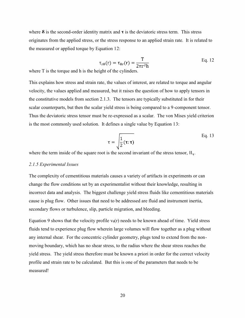
20

where is the second-order identity matrix and is the deviatoric stress term. This stress

originates from the applied stress, or the stress response to an applied strain rate. It is related to

the measured or applied torque by Equation 12:

τ (r) = τ (r) = T2πr h Eq. 12

where T is the torque and h is the height of the cylinders.

This explains how stress and strain rate, the values of interest, are related to torque and angular

velocity, the values applied and measured, but it raises the question of how to apply tensors in

the constitutive models from section 2.1.3. The tensors are typically substituted in for their

scalar counterparts, but then the scalar yield stress is being compared to a 9-component tensor.

Thus the deviatoric stress tensor must be re-expressed as a scalar. The von Mises yield criterion

is the most commonly used solution. It defines a single value by Equation 13:

τ = 12 ( : ) Eq. 13

where the term inside of the square root is the second invariant of the stress tensor, II .

2.1.5 Experimental Issues

The complexity of cementitious materials causes a variety of artifacts in experiments or can

change the flow conditions set by an experimentalist without their knowledge, resulting in

incorrect data and analysis. The biggest challenge yield stress fluids like cementitious materials

cause is plug flow. Other issues that need to be addressed are fluid and instrument inertia,

secondary flows or turbulence, slip, particle migration, and bleeding.

Equation 9 shows that the velocity profile vθ(r) needs to be known ahead of time. Yield stress

fluids tend to experience plug flow wherein large volumes will flow together as a plug without

any internal shear. For the concentric cylinder geometry, plugs tend to extend from the non-

moving boundary, which has no shear stress, to the radius where the shear stress reaches the

yield stress. The yield stress therefore must be known a priori in order for the correct velocity

profile and strain rate to be calculated. But this is one of the parameters that needs to be

measured!

21

Wallevik et. al. describe a procedure using the Reiner-Riwlin equation that can overcome this

paradox33. The Reiner-Riwlin equation is used to transform data from angular velocity-torque

(W , T) format to a strain rate-stress (γ , τ) format. By substituting Equations 12 and 9 for the

stress and strain rate into the chosen constitutive model and integrating across the radial gap, the

constitutive model may be re-expressed in terms of torque and angular velocity. Equation 14

provides the equation for the Bingham model:

T = 4πh ∗ ln R R1R − 1R τ + 8π h1R − 1R μW Eq. 14

where Rs is the minimum of the outer cup radius Ro and the plug radius Rp where the velocity is

zero because the stress no longer exceeds the yield stress. Equation 15 provides the equation for

the Herschel-Bulkley model34:

T = 4πh ∗ ln R R1R − 1R τ + 2 π hKn 1R / − 1R / W Eq. 15

And Equation 16 provides the equation for the modified Bingham model33:

T = 4πh ∗ ln R R1R − 1R τ + 8π h1R − 1R μW + 8π h1R − 1R(R + R )(R − R ) cW Eq. 16

Wallevik et. al. state that the expression for the Bingham model may be simplified to Equation

17: T = G + HW Eq. 17

where G and H are constants that are determined by fitting data. They calculate the yield stress

and from their relationships to G and H using an iterative process. However, the process is

unclear and due to the presence of plug flow, G and H are not truly constants as the authors

imply. G and H are in fact functions of torque because they are functions of the outer radius Rs.

If the torque is large enough that the yield stress is achieved almost immediately at the cup

boundary, then Rs is simply Ro. However this cannot be known a priori and as such Equation 18

must be substituted into Equations 14 through 16:

22

R = min R , T2πτ h Eq. 18

The issue of plug flow can be overcome by fitting the (W , T) data to the new set of equations.

The fluid may experience inertial effects in addition to plug flow. When the spindle is applying

oscillatory shear at high frequencies or if the immediate response to an applied step stress is of

interest, then the sample’s inertia will cause propagating waves, either due to viscous momentum

diffusion or elastic shear waves35. The propagating waves must have a wavelength much larger

than the geometry gap in order for their effects to be negligible but defining the wavelength can

be challenging. The spindle may experience inertial effects under these conditions as well.

Changing the applied angular velocity quickly will require some additional torque, the quantity

being measured35. Some instruments are capable of correcting for this but others cannot

distinguish between the torque caused by the fluid and that caused by controlling the spindle. If

the instrument inertia is affecting the results, then the torque data will be proportional to the

time-derivative of the angular velocity, which is the acceleration. In this project, only steady

simple shear flow is used. No oscillatory shear is applied and whenever a step stress is applied,

the sample is given a long period of time to achieve a steady state flow, represented by a steady

torque. Thus inertia effects should not be an issue.

If the spindle is rotating at a high enough velocity, then inertial forces may cause instabilities,

secondary flows, and general turbulence. The analysis presented for the concentric cylinder

geometry relies on the assumption that the flow is laminar, which makes it easy to assume a

velocity profile. The Reynolds number is a dimensionless number that represents the ratio of the

inertial forces to the viscous forces and very high Reynolds numbers indicate that the flow is

turbulent while low Reynolds numbers indicate that the flow is laminar. Equation 19 gives the

Reynolds number for simple Newtonian fluids:

Re = ρvdη Eq. 19

where is the fluid density, v is the velocity, and d is a characteristic length. The Reynolds

number for yield stress fluids is still being investigated. Coussot recommends that at low strain

rates where the stress is on the same order as the yield stress, they be represented by Equation

2036:

23

Re = ρvτ Eq. 20

At high strain rates, the behavior can often be considered Newtonian and so Equation 19 is used

once again.

The concentric cylinder geometry is slightly unique because it is susceptible to axisymmetric

vortices, a well-known instability called Taylor-Couette flow35. As such the stability criteria

used for Newtonian fluids in concentric cylinder geometries is actually the Taylor number, given

in Equation 21 below:

Ta = ρ (R − R ) Rη < 1700 Eq. 21

Again, the Taylor number for yield stress fluids is not well-defined. However, since the Taylor

number is synonymous to the Reynolds number, it may be reasonable to adjust it in a manner

synonymous to the one suggested by Coussot.

Slip is another typical issue with cementitious materials and like plug flow, causes incorrect and

unknown boundary conditions. If the fluid slips at the boundaries, then it is not rotating at the

applied angular velocity and the true velocity is unknown. To prevent slip, the surfaces are often

roughened either with sandpaper or by sandblasting, or manufactured with machined grooves.

The grooves must be at least the size of the largest particle in the fluid to be effective. If they are

too small, then they will be filled with the interstitial fluid, which does not represent the material

correctly and will behave as a lubrication layer. Four-bladed vanes, eight-bladed vanes, and

vanes with even more blades may be used in place of cylindrical spindles to overcome severe

slip without changing the analytical steps, but they are susceptible to hydrodynamic pressure.

Hydrodynamic pressure on the flat surfaces of the blades will increase the torque for all shear

rates, and its effect increases with increasing shear rate37. Hydrodynamic pressure must be

corrected for if vane geometry is used.

Finally, suspensions suffer from particle settling and migration. When perturbed, denser grains

will sink to the bottom and lighter grains may float to the top of the fluid. During shear, grains

tend to migrate to areas of lower stress. Both of these events cause the formerly homogeneous

fluid to become heterogeneous. For concentric cylinder geometry, the largest particles will be

found at the non-moving boundary and at the bottom of the specimen. As the radius and depth

24

decrease, the particle size will become smaller. As such the yield stress and viscosity of the fluid

at the non-moving boundary would be greater than those of the fluid at the moving boundary;

that is, they become a function of position. This is most commonly seen in granular suspensions.

However, settlement can be a big issue for colloidal suspensions as well. In cement paste, this is

called bleeding because the colloids will settle, creating a highly viscous, grainy material in the

bottom of the cylinder, and bleed, leaving a layer of water on top of the sample. The denser

portion will cause the torque to increase falsely. Particle settling and migration cannot be

avoided but there are several steps that may be taken to minimize their effects. Colloidal

suspensions must be mixed well and watched closely during the experiment. The sample should

be disturbed as little as possible and measurements need to be taken quickly. Additionally,

concentric cylinders are not as susceptible to settling35 as other geometries.

2.2 Rheology of Vibrated Granular Suspensions

Very little literature on the rheology of vibrated concrete exists and rheologists have only begun

to study the rheology of vibrated granular suspensions in recent years. Most studies focus on

granular suspensions made of small, ideal spheres suspended in a Newtonian interstitial fluid.

The spherical grains typically have only one or two diameters on the order of a few micrometers

to a few millimeters. These materials are easy to work with because they only require small

sample sizes, making the equipment more manageable, and they limit the factors that may affect

behavior, making experiments easier to analyze and model. In contrast, the interstitial fluid for

concrete is a viscoelastic, thixotropic yield stress fluid and the grains vary from a few

nanometers (dust) to a few centimeters (gravel) in diameter. The aggregates have shape and

texture as well. These additional variables and behaviors cause variability and complicate

analysis, but the underlying behavior of concrete and idealized granular suspensions is the same.

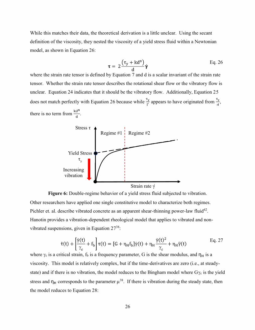
When subjected to vibration, the yield stress and viscosity are decreased at small strain rates38.

Figure 6 below illustrates this behavior. The dashed black line represents a granular suspension

that is not subjected to vibration while the solid black line represents one that has been subjected

to vibration. The suspension follows a Bingham model for simplicity. At low strain rates, the

vibrated suspension exhibits Newtonian behavior but rejoins the Bingham model at high strain

rates. Some papers distinguish between these two behaviors by assigning two regimes39,40. In

the first regime, the flow is vibration-controlled and the viscosity decreases with increasing

25

vibration40. To evaluate the extent of the vibration’s effect, Hanotin et. al. use a dimensionless

value called the Peclet number, given in Equation 2239:

Pe = η A(2πf)μ∆ρøgzd Eq. 22

where η is the viscosity of the interstitial fluid, μ is the friction coefficient between the grains,∆ρ is the density difference between the grains and the interstitial fluid, ø is the coarse particle

volume fraction, g is the gravitational constant, z is the average measurement depth, and d is the

grain diameter. The Peclet number is the ratio of the repulsion between the grains due to

lubrication to the friction between the grains. If the Peclet number is greater than one, then the

vibration successfully overcomes the friction. The Peclet number only applies to the first

regime; in the second regime, the flow is friction-controlled regardless of the presence of

vibration. Hanotin et. al. state that the boundary between the regimes is defined by the frictional

stress between the aggregates39. By applying Coulomb’s law, the frictional stress is determined

by Equation 23: σ = μP = μ∆ρøgz Eq. 23

where Pg is the pressure between the grains. In contrast, Ovarlez et. al. define the regime

boundary using the strain rate rather than the stress41. They treat vibration as a secondary flow

with a separate strain rate, , and state that this introduces a relaxation timescale, given by

Equation 24: λ = 1

Eq. 24

Synonymously, the first flow described by strain rate γ also has a relaxation timescale λ that is

the inverse of the strain rate. If λ is less than λ , then the material fully relaxes within the

timescale of the shear flow, permitting viscous flow. If λ is greater than λ , then the material

still experiences glassy behavior41, i.e., has a yield stress.

Ovarlez et. al. continue to assert the constitutive equation given in Equation 25 for the first

regime:

τ = τ

γ Eq. 25

26

While this matches their data, the theoretical derivation is a little unclear. Using the secant

definition of the viscosity, they nested the viscosity of a yield stress fluid within a Newtonian

model, as shown in Equation 26:

= 2 τ + kdd Eq. 26

where the strain rate tensor is defined by Equation 7 and d is a scalar invariant of the strain rate

tensor. Whether the strain rate tensor describes the rotational shear flow or the vibratory flow is

unclear. Equation 24 indicates that it should be the vibratory flow. Additionally, Equation 25

does not match perfectly with Equation 26 because while

appears to have originated from ,

there is no term from .

Figure 6: Double-regime behavior of a yield stress fluid subjected to vibration.

Other researchers have applied one single constitutive model to characterize both regimes.

Pichler et. al. describe vibrated concrete as an apparent shear-thinning power-law fluid42.

Hanotin provides a vibration-dependent rheological model that applies to vibrated and non-

vibrated suspensions, given in Equation 2738:

τ(t) + γ(t)

+ f τ(t) = [G + η f ]γ(t) + η γ(t)

+ η γ(t) Eq. 27

where c is a critical strain, fb is a frequency parameter, G is the shear modulus, and η is a

viscosity. This model is relatively complex, but if the time-derivatives are zero (i.e., at steady-

state) and if there is no vibration, the model reduces to the Bingham model where Gc is the yield

stress and η corresponds to the parameter 38. If there is vibration during the steady state, then

the model reduces to Equation 28:

Stress τ

Strain rate γ

Yield Stressτy

Regime #1 Regime #2

Increasingvibration

27

τ = Gγ + η f γγ + f γ γ + ηγ + f γ γ Eq. 28

And as the strain rate approaches zero, the model becomes Newtonian with a viscosity given by

Equation 2937:

η = Gf + η Eq. 29

This somewhat agrees with the viscosity used in Equation 25. The first term is related to the

yield stress and the frequency parameter is related to . But Equation 29 also includes the

second term that had been missing in Equation 25. This discussion highlights the fact that while

there is general agreement on the behavior of granular suspensions under vibration, there is no

well-established, common quantitative model yet.

The frequency parameter in the Hanotin model raises the important point of how to characterize

the vibration. Vibration is described by two parameters, its amplitude and frequency. Hanotin

et. al. combine these parameters into a single value for convenience and distinguish between

different vibration scenarios by the vibration stress, given as Equation 3039:

σ = 12 ρ(2πf) A Eq. 30

where f is the frequency and A is the displacement amplitude. The vibration stress is simply the

mechanical energy input by the vibrator per unit volume. The vibrator is considered a harmonic

oscillator and its total energy is the sum of its elastic potential energy and kinetic energy. This is

an attractive way to characterize the vibration but may not be practical for large samples and

fluids in which vibration does not propagate easily. In these situations, the amplitude and

vibration stress will vary with position, creating an unknown profile. Concrete is particularly

susceptible to this. It is typically vibrated by a vertical probe and the probe induces shear waves,

which are attenuated in entirely viscous fluids. Because concrete is mostly viscous in its early-

age, fresh state, the probe only affects the surrounding material. This vibrated volume has been

called the cone of action38. The cone shape originates from the weight of the material. At larger

depths, the hydrostatic pressure of the concrete provides confinement and makes it increasingly

difficult to vibrate the aggregates.

28

CHAPTER 3: CHALLENGES OF CHARACTERIZING CONCRETE RHEOLOGY

The ICAR (International Center for Aggregate Research) rheometer, developed by Eric Koehler,

is a rugged, portable piece of equipment used to measure the rheological properties of concrete43.

While user-friendly and useful, it has limitations. The series of experiments presented in this

chapter was conducted to become familiar with the limitations of the ICAR rheometer and

preempt any issues when studying vibrated concrete. The first section of the chapter describes

the experimental methods, the second discusses the results, and the final section discusses their

implications.

3.1 Experimental Methods

The following procedures explain the mixture designs and mixing procedure, the slump test, and

the two rheological tests conducted by the ICAR rheometer. Any deviations from standard

procedures are identified.

3.1.1 Mixture Designs and Mixing Procedure

All concrete mixtures were made using Type I/II Portland cement, tap water, Class F fly ash,

natural sand, and coarse limestone. The two aggregate stocks were characterized prior to design

in accordance with ASTM C127-15, the Standard Test Method for Relative Density (Specific

Gravity) and Absorption of Coarse Aggregate, and ASTM C128-15, the Standard Test Method

for Relative Density (Specific Gravity) and Absorption of Fine Aggregate. Each mixture had a

water-to-cement (w/c) ratio of 0.35 and a 25%wt fly ash replacement. The water content was

varied in order to produce concretes with different slumps. The fraction of coarse aggregates in

the concrete remained the same for each mixture while the fraction of fine aggregates was

decreased to account for increasing the paste content. An air content of 3% was assumed for all

mixtures. The final mixture designs are given in Table 1.

A large mixer (Lancaster Products, Type 30-DP, year 2011, number 224) by Kercher Industries,

Inc. was used for concrete mixing. The pan was first wetted so its surface was lightly damp.

The aggregates were measured into the pan, about half of the water was poured in, and they were

mixed for 30 seconds. The cement and any mineral additives were then poured into the pan and

the mixture was mixed for 2 minutes, during which the rest of the water was poured in. The

mixture was then given one minute to rest and some of it was turned over by hand to help

29

distribute the cement paste at the bottom of the pan. Finally, the mixture was mixed for one

more minute. The total mixing time was 4 minutes and 30 seconds.

Table 1: Concrete mixtures belonging to Series 1.

Mixture ID w Water Cement Fly ashCoarse

LimestoneNaturalSand

-- lb/yd3 lb lb lb lb lbCLS240 240 14.97 24.76 8.25 82.23 60.77CLS270 270 16.3 27.86 9.29 83.34 53.47CLS285 285 16.96 29.4 9.8 82.23 49.82CLS315 315 18.29 32.5 10.83 82.23 42.53CLS330 330 18.95 34.05 11.35 82.23 38.88CLS360 360 20.28 37.14 12.38 82.23 31.58

3.1.2 Slump Test

The slump test was conducted for every fresh concrete batch in accordance with ASTM C143. It

was done between a hydration age of 5 and 15 minutes.

3.1.3 ICAR Rheometer Tests: Stress Growth and Flow Curve

An ICAR rheometer from Germann Instruments was used for rheological tests on concrete. The

ICAR rheometer is capable of stress growth tests and flow sweep (aka, flow curve) tests. The

bucket was 30.48 cm in diameter and had ridges running vertically along the inside that were

1.27-cm thick and wide to prevent slip. The spindle was a 4-bladed vane with a 12.7-cm

diameter and a height of 12.6 cm. The vane could rotate at angular speeds between 0.01 and

0.60 revolutions per second (rev/s) and the torque meter was capable of measuring torques up to

25 N-m.

The torque was zeroed prior to each measurement. The concrete was placed in the ICAR bucket

in two lifts and each lift was rodded 25 times. Immediately after placing the concrete, the

spindle and torque meter assembly was lowered into position with the spindle kept as vertical as

possible. The concrete was left undisturbed until a hydration age of 15 minutes. At 15 minutes,

the stress growth test was conducted. The flow curve test was conducted immediately after the

stress growth test was finished.

30

Stress growth tests measure the static yield stress of the concrete. The spindle was rotated at an

angular velocity of 0.025 rev/s and the test was stopped when the torque began to decrease

steadily or after 20 seconds, whichever occurred first. The maximum torque was converted to

static yield stress using Equation 31 below44:

τ = 2TπD HD + 13 Eq. 31

where D is the diameter of the vane, H is the height of the vane, and T is the maximum torque.

Flow sweep tests measure the -parameter and dynamic yield stress of concrete. Immediately

after the stress growth test was stopped, the concrete was presheared at a rate of 0.5 rev/s for 20

seconds. The rheometer then took 7 datapoints at angular velocities equally spaced between 0.50

rev/s and 0.05 rev/s with 5 seconds of data collection per point. The software used the Reiner-

Riwlin equation to fit the data to the Bingham model.

3.2 Results and Discussion

Figure 7 plots the three rheological parameters of the concretes against their slumps. The

specific values for the results are given in Table 2. There has been considerable discussion over

the value of the slump test. While practical, it summarizes concrete rheology with a single value

whereas all the applicable constitutive models require at least two. Figure 7 shows that overall

there is a strong correlation between yield stress and slump, particularly regarding the dynamic

yield stress. The only point that does not support this is CLS315. This mixture had an

unexpectedly large slump and static yield stress, although its dynamic yield stress agreed well

with the dynamic yield stress of the other mixture that had 8.5 inches of slump, CLS360.

Table 2: Specific values for the yield stresses and viscosity plotted in Figure 7.

Mixture IDSlump(in.)

Static yieldstress (Pa)

Dynamic yieldstress (Pa)

Viscosity(Pa-s)

CLS240 2.5 5986CLS270 4 2554 682.5 57.1CLS285 5.5 2045 645.8 22.6CLS315 8.5 1815 350.0 31.0CLS330 6.9 1735 425.4 38.1CLS360 8.5 1160 357.9 24.9

31

Figure 7: The static and dynamic yield stresses and viscosity of the Series 1 mixtures plottedagainst their slumps.

The -parameter from the Bingham model however only shows a very weak negative correlation

with the slump. The negative relationship is expected, but the extreme scatter in the data is not.

The most likely explanation is the poor control of the amount of dust in the coarse limestone

stock. Certain volumes of the stock are nothing but dust and fine aggregates while other parts

are entirely coarse aggregates. The stock was sampled as uniformly as possible, but the amount

of dust was likely highly variable between the mixtures. Another explanation may be the

sensitivity of the ICAR rheometer. However, the ICAR has exhibited good repeatability and so

the dust is the more likely culprit.

For CLS240, no dynamic yield stress or viscosity could be determined. The slump was large

enough that the torque meter was not strong enough to cause flow. This was expected as the

ICAR rheometer’s manual states that the instrument cannot measure the properties of concretes

with slumps less than 2 or 3 inches. A preliminary no-slump mixture further demonstrated this

since not even a static yield stress could be determined. As shown in Figure 8, this no-slump

mixture underwent a phenomenon called “shear localization” in rheology wherein a very thin

band of the material experienced uniquely high rates of shear. The material could not sustain

such high shears and essentially fractured. Any torque readings were caused by the friction

0

10

20

30

40

50

60

0

1000

2000

3000

4000

5000

6000

7000

2 3 4 5 6 7 8 9

fr

om B

ingh

am M

odel

(Pa-

s)

Yiel

d St

ress

es (P

a)

Slump (in.)

Static Yield Stress (Pa) Dynamic Yield Stress (Pa) mu (Bingham) (Pa-s)

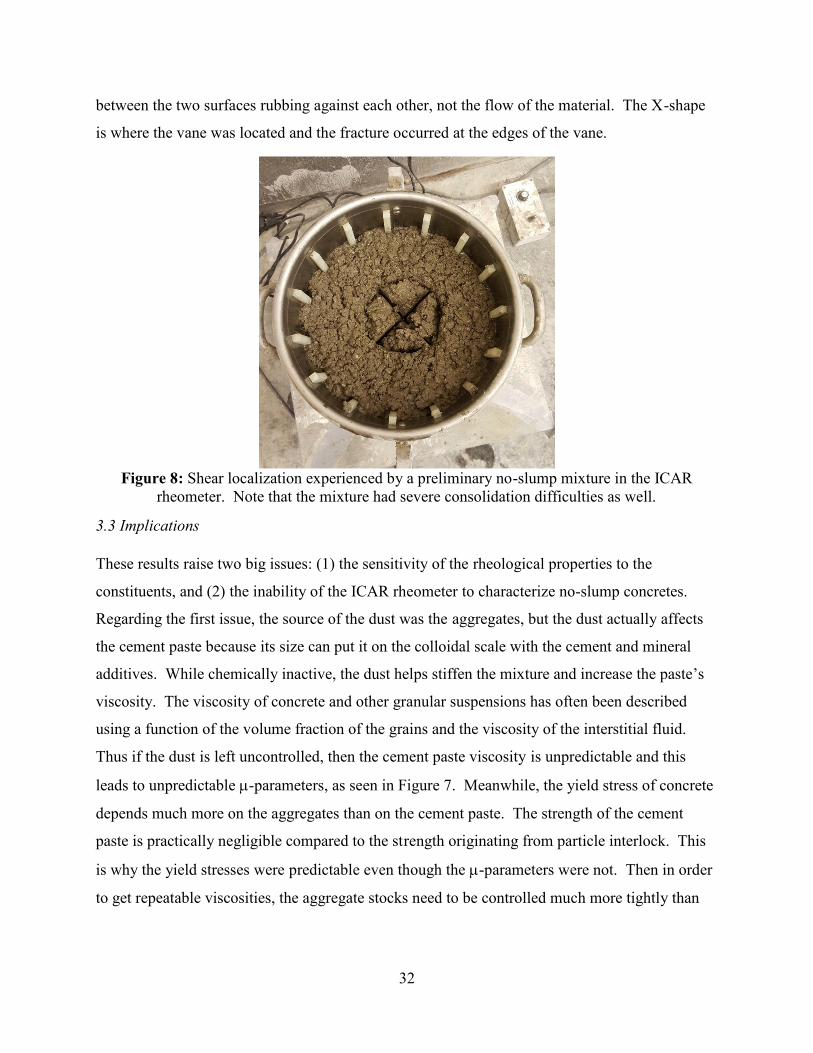
32

between the two surfaces rubbing against each other, not the flow of the material. The X-shape

is where the vane was located and the fracture occurred at the edges of the vane.

Figure 8: Shear localization experienced by a preliminary no-slump mixture in the ICARrheometer. Note that the mixture had severe consolidation difficulties as well.

3.3 Implications

These results raise two big issues: (1) the sensitivity of the rheological properties to the

constituents, and (2) the inability of the ICAR rheometer to characterize no-slump concretes.

Regarding the first issue, the source of the dust was the aggregates, but the dust actually affects

the cement paste because its size can put it on the colloidal scale with the cement and mineral

additives. While chemically inactive, the dust helps stiffen the mixture and increase the paste’s

viscosity. The viscosity of concrete and other granular suspensions has often been described

using a function of the volume fraction of the grains and the viscosity of the interstitial fluid.

Thus if the dust is left uncontrolled, then the cement paste viscosity is unpredictable and this

leads to unpredictable -parameters, as seen in Figure 7. Meanwhile, the yield stress of concrete

depends much more on the aggregates than on the cement paste. The strength of the cement

paste is practically negligible compared to the strength originating from particle interlock. This

is why the yield stresses were predictable even though the -parameters were not. Then in order

to get repeatable viscosities, the aggregate stocks need to be controlled much more tightly than

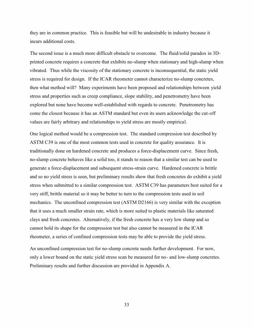
33

they are in common practice. This is feasible but will be undesirable in industry because it

incurs additional costs.

The second issue is a much more difficult obstacle to overcome. The fluid/solid paradox in 3D-

printed concrete requires a concrete that exhibits no-slump when stationary and high-slump when

vibrated. Thus while the viscosity of the stationary concrete is inconsequential, the static yield

stress is required for design. If the ICAR rheometer cannot characterize no-slump concretes,

then what method will? Many experiments have been proposed and relationships between yield

stress and properties such as creep compliance, slope stability, and penetrometry have been

explored but none have become well-established with regards to concrete. Penetrometry has

come the closest because it has an ASTM standard but even its users acknowledge the cut-off

values are fairly arbitrary and relationships to yield stress are mostly empirical.

One logical method would be a compression test. The standard compression test described by

ASTM C39 is one of the most common tests used in concrete for quality assurance. It is

traditionally done on hardened concrete and produces a force-displacement curve. Since fresh,

no-slump concrete behaves like a solid too, it stands to reason that a similar test can be used to

generate a force-displacement and subsequent stress-strain curve. Hardened concrete is brittle

and so no yield stress is seen, but preliminary results show that fresh concretes do exhibit a yield

stress when submitted to a similar compression test. ASTM C39 has parameters best suited for a

very stiff, brittle material so it may be better to turn to the compression tests used in soil

mechanics. The unconfined compression test (ASTM D2166) is very similar with the exception

that it uses a much smaller strain rate, which is more suited to plastic materials like saturated

clays and fresh concretes. Alternatively, if the fresh concrete has a very low slump and so

cannot hold its shape for the compression test but also cannot be measured in the ICAR

rheometer, a series of confined compression tests may be able to provide the yield stress.

An unconfined compression test for no-slump concrete needs further development. For now,

only a lower bound on the static yield stress scan be measured for no- and low-slump concretes.

Preliminary results and further discussion are provided in Appendix A.

34

CHAPTER 4: RHEOLOGY OF VIBRATED CONCRETE

The previous chapter focused on non-vibrated concretes that followed traditional mixture

designs. This chapter focuses on the vibrated, no-slump concretes required to solve the

fluid/solid paradox in 3D printing and how to describe them rheologically. The first section

describes the experimental procedures, the second presents the results, and the third and final

section discusses the benefits and drawbacks of several different analyses.

4.1 Experimental Methods

The following subsections explain how the methods from Chapter 3 were adapted to

accommodate the study of vibrating granular suspensions. The first explains the mixture designs

and the second explains how the mixtures were subjected to vibration during rheological

experiments.

4.1.1 Mixture Designs and Mixing Procedure

The concrete mixtures used in this series of tests were designed to mimic the granular

suspensions seen in literature with concrete constituents, and the constituents were closely

controlled to avoid variability as discussed in section 3.3. A stable cement paste mixture was

designed first with Type I/II Portland cement, silica fume, and water. Table 3 provides the

mixtures that were considered. Each was subjected to a stability test. During batching for

cement pastes, the cement was sieved through flour sifter to ensure there were no clumps. The

cement and silica fume were poured into a wetted mixing bowl. The water was added in parts

and mixed in by hand with a spatula for the first 4 minutes and 30 seconds to prevent the

constituents from flying out of the bowl. Once as homogeneous as possible, the bowl was

latched into a three-speed KitchenAid mixer and a whisk was attached. The mixture was mixed

at a low speed for one minute, then at the middle speed for one minute, and then at the top speed.

If the mixture splashed at higher speeds, then the lower speeds were used instead. Finally, the

mixture was mixed at the low speed for the final minute. The complete mixing procedure time

was 9 minutes for cement pastes. Once mixed, the paste was poured into two 100-ml graduated

cylinders to the 100-ml mark. At hydration ages of 30 minutes and 1 hour, the amount of bleed

water was recorded to the nearest tenth of a milliliter. CP2 was highly resistant to bleeding and

was subsequently used in the concrete mixture designs.

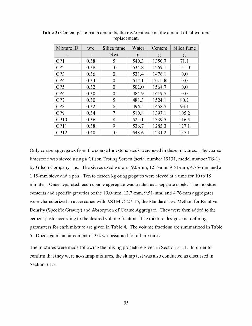
35

Table 3: Cement paste batch amounts, their w/c ratios, and the amount of silica fumereplacement.

Mixture ID w/c Silica fume Water Cement Silica fume-- -- %wt g g g

CP1 0.38 5 540.3 1350.7 71.1CP2 0.38 10 535.8 1269.1 141.0CP3 0.36 0 531.4 1476.1 0.0CP4 0.34 0 517.1 1521.00 0.0CP5 0.32 0 502.0 1568.7 0.0CP6 0.30 0 485.9 1619.5 0.0CP7 0.30 5 481.3 1524.1 80.2CP8 0.32 6 496.5 1458.5 93.1CP9 0.34 7 510.8 1397.1 105.2CP10 0.36 8 524.1 1339.5 116.5CP11 0.38 9 536.7 1285.3 127.1CP12 0.40 10 548.6 1234.2 137.1

Only coarse aggregates from the coarse limestone stock were used in these mixtures. The coarse

limestone was sieved using a Gilson Testing Screen (serial number 19131, model number TS-1)

by Gilson Company, Inc. The sieves used were a 19.0-mm, 12.7-mm, 9.51-mm, 4.76-mm, and a

1.19-mm sieve and a pan. Ten to fifteen kg of aggregates were sieved at a time for 10 to 15

minutes. Once separated, each coarse aggregate was treated as a separate stock. The moisture

contents and specific gravities of the 19.0-mm, 12.7-mm, 9.51-mm, and 4.76-mm aggregates

were characterized in accordance with ASTM C127-15, the Standard Test Method for Relative

Density (Specific Gravity) and Absorption of Coarse Aggregate. They were then added to the

cement paste according to the desired volume fraction. The mixture designs and defining

parameters for each mixture are given in Table 4. The volume fractions are summarized in Table

5. Once again, an air content of 3% was assumed for all mixtures.

The mixtures were made following the mixing procedure given in Section 3.1.1. In order to

confirm that they were no-slump mixtures, the slump test was also conducted as discussed in

Section 3.1.2.

36

Table 4: Concrete mixtures belonging to Series 2. Each mixture had a w/c ratio of 0.28 and a10%wt silica fume replacement (CP2).

Mixture ID Water CementSilicafume

19.0-mmLimestone

12.7-mmLimestone

9.51-mmLimestone

4.76-mmLimestone

-- lb lb lb lb lb lb lbH 13.74 27.56 3.06 0 102.13 0 0TE 13.09 24.97 2.77 0 0 106.39 0N4 13.59 25.83 2.87 0 0 0 102.76H&N4 13.25 25.83 2.87 0 70.53 0 33.91TE&N4 13.48 25.83 2.87 0 0 70.23 33.91All67 13.34 25.83 2.87 10.66 15.79 31.45 46.24All57 16.67 34.45 3.83 9.07 13.43 26.75 39.34

Table 5: The volume fractions of each sized aggregate for the mixtures from Table 4.

Mixture IDTotal

coarse agg.19.0-mmLimestone

12.7-mmLimestone

9.51-mmLimestone

4.76-mmLimestone

-- %vol %vol %vol %vol %volH 65 0 100 0 0TE 68 0 0 100 0N4 67 0 0 0 100H&N4 67 0 67 0 33TE&N4 67 0 0 67 33All67 67 10 15 30 45All57 57 10 15 30 45

4.1.2 Adding Vibration to the ICAR Rheometer Tests

The stress growth and flow curve tests were measured with the same parameters as discussed in

Section 3.1.3. The primary difference is that the bucket was placed on a vibration table and the

torque meter rested on a stand just above the bucket during measurements to prevent the ICAR

device from feeling the vibration. The vibration table was turned on before starting any

rheological tests and turned off once the tests were completed. These mixtures were also

difficult to consolidate so each lift was vibrated for a few seconds after rodding. Figure 9 shows

the set-up. The vibration table used was a Vibco table (Model US-900, Serial number 042267)

37

that operated at one amplitude (>1.2 mm) and frequency (143.5 Hz). The bucket was clamped to

the surface using two Husky ratchet clamps.

Figure 9: Image of the experimental set-up for vibrated, no-slump concretes during rheologicaltesting.

4.1.3 Characterizing Vibration

The frequency and amplitude experienced by the concrete in the bucket was measured with

triaxial ICP® accelerometers (model 356A32) and a four-channel, ICP® Sensor Signal

Conditioner (model 482C05) by PCB Piezotronics. A LabVIEW (National InstrumentsTM)

program was used to control them. The accelerometer was wrapped in Ceram wrap and the wire

was passed through a plastic, cylindrical tube to protect it during testing. It was placed at 25

different locations within the concrete-filled bucket as shown in the schematic in Figure 10. The

locations formed a grid and fully characterized a cross-section going through the center of the

bucket. When the accelerometer had to be placed at a certain depth, a tamping rod was used to

provide a hole for the accelerometer to be inserted into. The concrete was briefly vibrated

afterwards to help the concrete close the hole around the accelerometer and tube. The

accelerometer was also held against the surface of the vibration table to characterize the input

frequency and amplitude. The X direction coincided with the vertical.

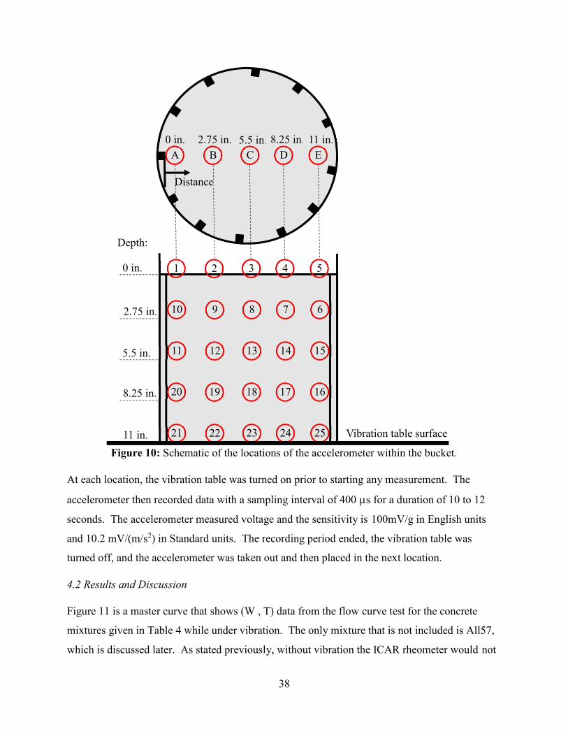
38

Figure 10: Schematic of the locations of the accelerometer within the bucket.

At each location, the vibration table was turned on prior to starting any measurement. The

accelerometer then recorded data with a sampling interval of 400 s for a duration of 10 to 12

seconds. The accelerometer measured voltage and the sensitivity is 100mV/g in English units

and 10.2 mV/(m/s2) in Standard units. The recording period ended, the vibration table was

turned off, and the accelerometer was taken out and then placed in the next location.

4.2 Results and Discussion

Figure 11 is a master curve that shows (W , T) data from the flow curve test for the concrete

mixtures given in Table 4 while under vibration. The only mixture that is not included is All57,

which is discussed later. As stated previously, without vibration the ICAR rheometer would not

25

5

15

6

16

21

1

11

10

20

23

3

13

8

18

24

4

14

7

17

22

2

12

9

19

EA C DB

Depth:

0 in.

2.75 in.

5.5 in.

8.25 in.

11 in.

0 in. 2.75 in. 5.5 in. 8.25 in. 11 in.

Distance

Vibration table surface

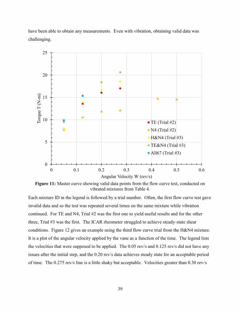
39

have been able to obtain any measurements. Even with vibration, obtaining valid data was

challenging.

Figure 11: Master curve showing valid data points from the flow curve test, conducted onvibrated mixtures from Table 4.

Each mixture ID in the legend is followed by a trial number. Often, the first flow curve test gave

invalid data and so the test was repeated several times on the same mixture while vibration

continued. For TE and N4, Trial #2 was the first one to yield useful results and for the other

three, Trial #3 was the first. The ICAR rheometer struggled to achieve steady-state shear

conditions. Figure 12 gives an example using the third flow curve trial from the H&N4 mixture.

It is a plot of the angular velocity applied by the vane as a function of the time. The legend lists

the velocities that were supposed to be applied. The 0.05 rev/s and 0.125 rev/s did not have any

issues after the initial step, and the 0.20 rev/s data achieves steady state for an acceptable period

of time. The 0.275 rev/s line is a little shaky but acceptable. Velocities greater than 0.30 rev/s

0

5

10

15

20

25

0 0.1 0.2 0.3 0.4 0.5 0.6

Torq

ue T

(N-m

)

Angular Velocity W (rev/s)

TE (Trial #2)N4 (Trial #2)H&N4 (Trial #3)TE&N4 (Trial #3)All67 (Trial #3)

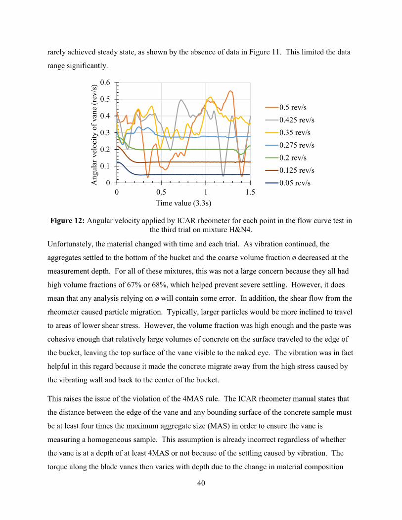
40

rarely achieved steady state, as shown by the absence of data in Figure 11. This limited the data

range significantly.

Figure 12: Angular velocity applied by ICAR rheometer for each point in the flow curve test inthe third trial on mixture H&N4.

Unfortunately, the material changed with time and each trial. As vibration continued, the

aggregates settled to the bottom of the bucket and the coarse volume fraction ø decreased at the

measurement depth. For all of these mixtures, this was not a large concern because they all had

high volume fractions of 67% or 68%, which helped prevent severe settling. However, it does

mean that any analysis relying on ø will contain some error. In addition, the shear flow from the

rheometer caused particle migration. Typically, larger particles would be more inclined to travel

to areas of lower shear stress. However, the volume fraction was high enough and the paste was

cohesive enough that relatively large volumes of concrete on the surface traveled to the edge of

the bucket, leaving the top surface of the vane visible to the naked eye. The vibration was in fact

helpful in this regard because it made the concrete migrate away from the high stress caused by

the vibrating wall and back to the center of the bucket.

This raises the issue of the violation of the 4MAS rule. The ICAR rheometer manual states that

the distance between the edge of the vane and any bounding surface of the concrete sample must

be at least four times the maximum aggregate size (MAS) in order to ensure the vane is

measuring a homogeneous sample. This assumption is already incorrect regardless of whether

the vane is at a depth of at least 4MAS or not because of the settling caused by vibration. The

torque along the blade vanes then varies with depth due to the change in material composition

0

0.1

0.2

0.3

0.4

0.5

0.6

0 0.5 1 1.5

Ang

ular

vel

ocity

of v

ane

(rev/

s)

Time value (3.3s)

0.5 rev/s0.425 rev/s0.35 rev/s0.275 rev/s0.2 rev/s0.125 rev/s0.05 rev/s

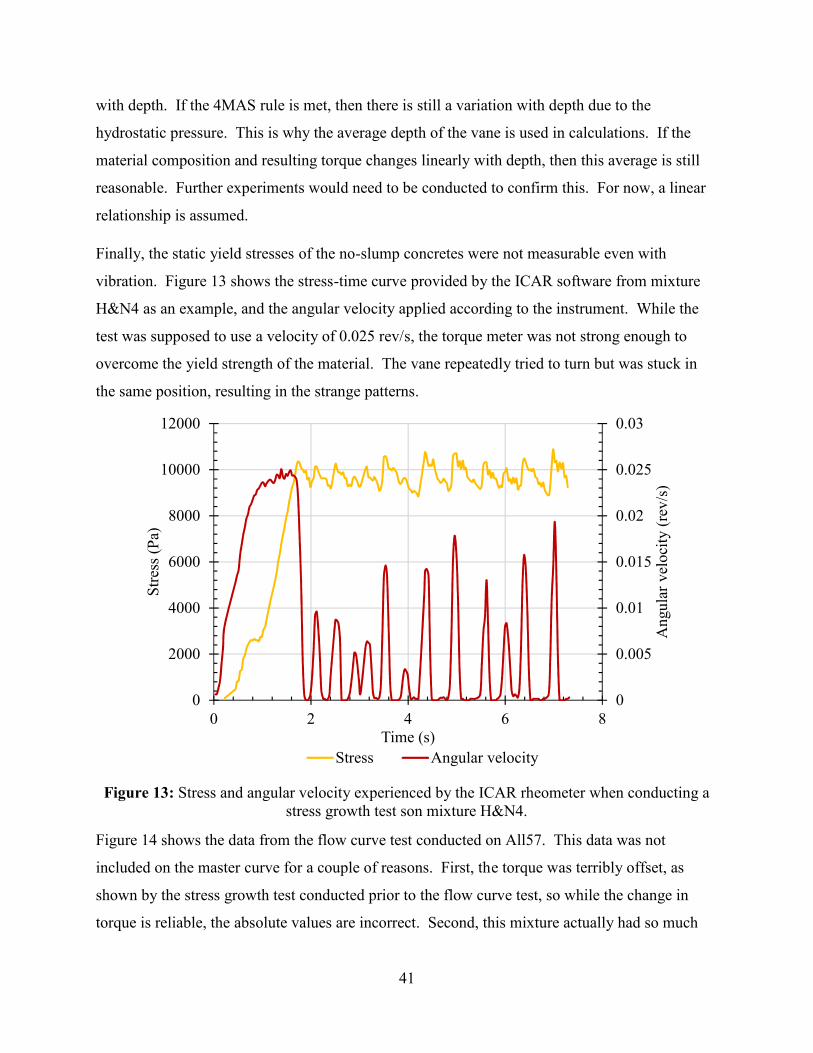
41

with depth. If the 4MAS rule is met, then there is still a variation with depth due to the

hydrostatic pressure. This is why the average depth of the vane is used in calculations. If the

material composition and resulting torque changes linearly with depth, then this average is still

reasonable. Further experiments would need to be conducted to confirm this. For now, a linear

relationship is assumed.

Finally, the static yield stresses of the no-slump concretes were not measurable even with

vibration. Figure 13 shows the stress-time curve provided by the ICAR software from mixture

H&N4 as an example, and the angular velocity applied according to the instrument. While the

test was supposed to use a velocity of 0.025 rev/s, the torque meter was not strong enough to

overcome the yield strength of the material. The vane repeatedly tried to turn but was stuck in

the same position, resulting in the strange patterns.

Figure 13: Stress and angular velocity experienced by the ICAR rheometer when conducting astress growth test son mixture H&N4.

Figure 14 shows the data from the flow curve test conducted on All57. This data was not

included on the master curve for a couple of reasons. First, the torque was terribly offset, as

shown by the stress growth test conducted prior to the flow curve test, so while the change in

torque is reliable, the absolute values are incorrect. Second, this mixture actually had so much

0

0.005

0.01

0.015

0.02

0.025

0.03

0

2000

4000

6000

8000

10000

12000

0 2 4 6 8

Ang

ular

vel

ocity

(rev

/s)

Stre

ss (P

a)

Time (s)Stress Angular velocity

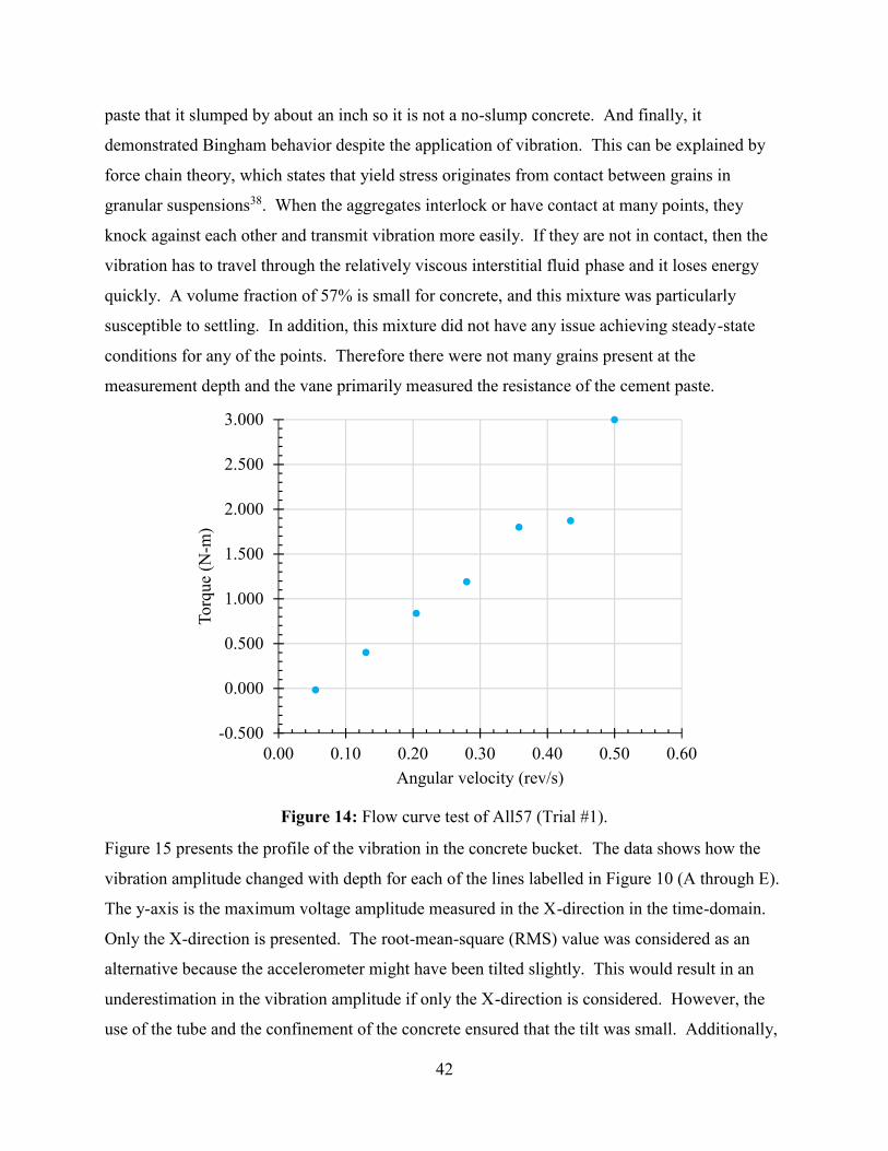
42

paste that it slumped by about an inch so it is not a no-slump concrete. And finally, it

demonstrated Bingham behavior despite the application of vibration. This can be explained by

force chain theory, which states that yield stress originates from contact between grains in

granular suspensions38. When the aggregates interlock or have contact at many points, they

knock against each other and transmit vibration more easily. If they are not in contact, then the

vibration has to travel through the relatively viscous interstitial fluid phase and it loses energy

quickly. A volume fraction of 57% is small for concrete, and this mixture was particularly

susceptible to settling. In addition, this mixture did not have any issue achieving steady-state

conditions for any of the points. Therefore there were not many grains present at the

measurement depth and the vane primarily measured the resistance of the cement paste.

Figure 14: Flow curve test of All57 (Trial #1).

Figure 15 presents the profile of the vibration in the concrete bucket. The data shows how the

vibration amplitude changed with depth for each of the lines labelled in Figure 10 (A through E).

The y-axis is the maximum voltage amplitude measured in the X-direction in the time-domain.

Only the X-direction is presented. The root-mean-square (RMS) value was considered as an

alternative because the accelerometer might have been tilted slightly. This would result in an

underestimation in the vibration amplitude if only the X-direction is considered. However, the

use of the tube and the confinement of the concrete ensured that the tilt was small. Additionally,

-0.500

0.000

0.500

1.000

1.500

2.000

2.500

3.000

0.00 0.10 0.20 0.30 0.40 0.50 0.60

Torq

ue (N

-m)

Angular velocity (rev/s)

43

there were sources of vibration in the horizontal Z- and Y- directions which were not of interest

so X-values were deemed the most appropriate. Some of the time-domain plots have been

provided in Appendix B as supplementary information. A plot of the amplitude in the X-

direction against the distance across the bucket is included and discussed as well. The data was

inconclusive and further testing is needed to determine how the vibration varied radially.

Figure 15: The vibration amplitude profile of the concrete in the ICAR bucket during vibration.

Figure 16 presents the data for each of the accelerometer tests in the frequency domain. A fast

Fourier transform (FFT) was completed using a MATLABTM code provided in Appendix C. All

of the spectra have a large peak at about 140 Hz, which was taken to be the operating frequency

of the table. The specific frequencies are given in Table 6. Figure 16 also shows peaks at

regular intervals (280 Hz, 420 Hz, etc.) and these were determined to be overtones of the

operating frequency. The smaller peaks at frequencies below the operating frequency vary for

each of the tests within the ICAR bucket and are likely caused by the surrounding aggregates.

0

1

2

3

4

5

6

7

0 2 4 6 8 10 12

Am

plitu

de in

X (V

)

Depth (in.)

ABCDE

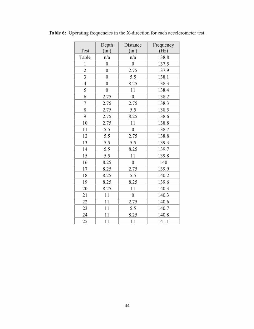
44

Table 6: Operating frequencies in the X-direction for each accelerometer test.

TestDepth(in.)

Distance(in.)

Frequency(Hz)

Table n/a n/a 138.81 0 0 137.52 0 2.75 137.93 0 5.5 138.14 0 8.25 138.35 0 11 138.46 2.75 0 138.27 2.75 2.75 138.38 2.75 5.5 138.59 2.75 8.25 138.6

10 2.75 11 138.811 5.5 0 138.712 5.5 2.75 138.813 5.5 5.5 139.314 5.5 8.25 139.715 5.5 11 139.816 8.25 0 14017 8.25 2.75 139.918 8.25 5.5 140.219 8.25 8.25 139.620 8.25 11 140.321 11 0 140.322 11 2.75 140.623 11 5.5 140.724 11 8.25 140.825 11 11 141.1

45

Figure 16: The frequency spectra of all the tests run by the accelerometer.

4.3 Further Analysis of Vibrated Rheological Behavior

The final section of Chapter 2 reviewed constitutive models that have been applied to or

proposed for vibrated granular suspensions in literature. This section applies them to the master

curve in Figure 11 and discusses how appropriate they are. The first subsection focuses on the

power-law fluid model and the second focuses on the Hanotin model. The final one discusses

some additional implications of the data from the vibration profile. Discussion of the Peclet

number used by Hanotin et. al. is included in Appendix D as supplementary information as it

requires more development.

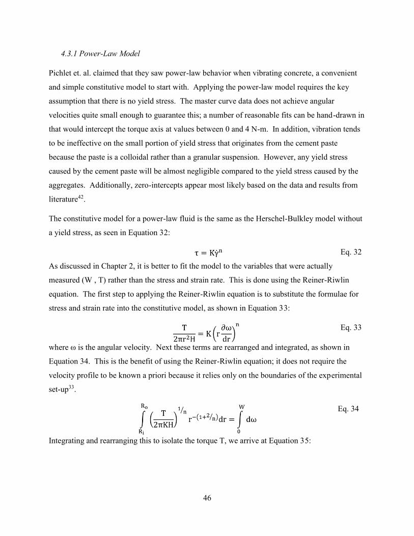
46

4.3.1 Power-Law Model

Pichlet et. al. claimed that they saw power-law behavior when vibrating concrete, a convenient

and simple constitutive model to start with. Applying the power-law model requires the key

assumption that there is no yield stress. The master curve data does not achieve angular

velocities quite small enough to guarantee this; a number of reasonable fits can be hand-drawn in

that would intercept the torque axis at values between 0 and 4 N-m. In addition, vibration tends

to be ineffective on the small portion of yield stress that originates from the cement paste

because the paste is a colloidal rather than a granular suspension. However, any yield stress

caused by the cement paste will be almost negligible compared to the yield stress caused by the

aggregates. Additionally, zero-intercepts appear most likely based on the data and results from

literature42.

The constitutive model for a power-law fluid is the same as the Herschel-Bulkley model without

a yield stress, as seen in Equation 32: τ = Kγ Eq. 32

As discussed in Chapter 2, it is better to fit the model to the variables that were actually

measured (W , T) rather than the stress and strain rate. This is done using the Reiner-Riwlin

equation. The first step to applying the Reiner-Riwlin equation is to substitute the formulae for

stress and strain rate into the constitutive model, as shown in Equation 33:T2πr H = K r ∂ωdr Eq. 33

where ω is the angular velocity. Next these terms are rearranged and integrated, as shown in

Equation 34. This is the benefit of using the Reiner-Riwlin equation; it does not require the

velocity profile to be known a priori because it relies only on the boundaries of the experimental

set-up33.

T2πKH r dr = dω Eq. 34

Integrating and rearranging this to isolate the torque T, we arrive at Equation 35:

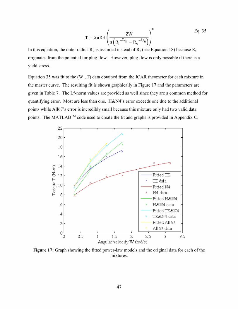
47

T = 2πKH 2Wn R − R Eq. 35

In this equation, the outer radius Ro is assumed instead of Rs (see Equation 18) because Rs

originates from the potential for plug flow. However, plug flow is only possible if there is a

yield stress.

Equation 35 was fit to the (W , T) data obtained from the ICAR rheometer for each mixture in

the master curve. The resulting fit is shown graphically in Figure 17 and the parameters are

given in Table 7. The L2-norm values are provided as well since they are a common method for

quantifying error. Most are less than one. H&N4’s error exceeds one due to the additional

points while All67’s error is incredibly small because this mixture only had two valid data

points. The MATLABTM code used to create the fit and graphs is provided in Appendix C.

Figure 17: Graph showing the fitted power-law models and the original data for each of themixtures.

48

Table 7: Parameters and errors for the power-law model for each of the mixtures.

Mixture ID K (Pa-sn) n L2-normTE 2526 0.323 0.324N4 1985 0.270 0.866H&N4 2326 0.458 1.227TE&N4 2627 0.437 0.653All67 2663 0.459 0.046

At first glance, the fit looks very good. Figure 18 extrapolates the fitted models to low and high

shear rates.

Figure 18: Power-law models extrapolated from strain rates of 0 to 100 s-1.

However, in literature on granular suspensions, there is general agreement that the fluids show

Newtonian behavior at low shear rates and return to their regular, non-vibrated behavior and

yield stress constitutive models at high shear rates. For concrete, this would imply that

Newtonian behavior is shown in the first regime and Bingham behavior is shown in the second

regime. The power-law model is incapable of mimicking either behavior. As the shear rate

approaches zero, the viscosity blows up to infinity rather than settling at a constant plateau. The

power-law model will also deviate from the Bingham model at high shear rates because its

power prevents it from ever demonstrating linear behavior. This may not be such a bad thing as

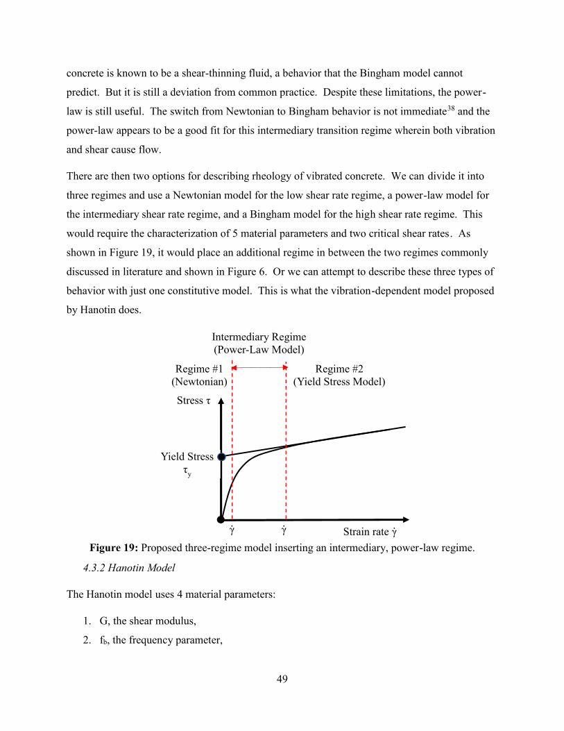
49

concrete is known to be a shear-thinning fluid, a behavior that the Bingham model cannot

predict. But it is still a deviation from common practice. Despite these limitations, the power-

law is still useful. The switch from Newtonian to Bingham behavior is not immediate38 and the

power-law appears to be a good fit for this intermediary transition regime wherein both vibration

and shear cause flow.

There are then two options for describing rheology of vibrated concrete. We can divide it into

three regimes and use a Newtonian model for the low shear rate regime, a power-law model for

the intermediary shear rate regime, and a Bingham model for the high shear rate regime. This

would require the characterization of 5 material parameters and two critical shear rates. As

shown in Figure 19, it would place an additional regime in between the two regimes commonly

discussed in literature and shown in Figure 6. Or we can attempt to describe these three types of

behavior with just one constitutive model. This is what the vibration-dependent model proposed

by Hanotin does.

Figure 19: Proposed three-regime model inserting an intermediary, power-law regime.

4.3.2 Hanotin Model

The Hanotin model uses 4 material parameters:

1. G, the shear modulus,

2. fb, the frequency parameter,

Stress τ

Strain rate γ

Yield Stressτy

Regime #1(Newtonian)

Regime #2(Yield Stress Model)

Intermediary Regime(Power-Law Model)

γ γ

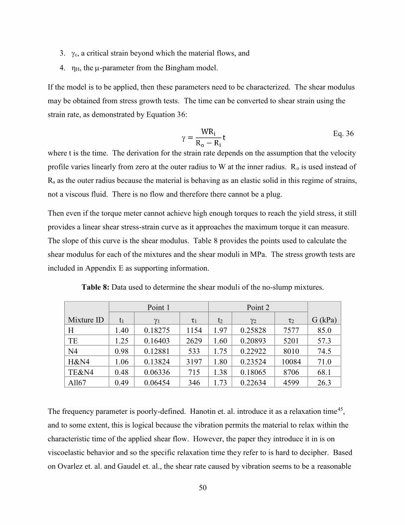
50

3. c, a critical strain beyond which the material flows, and

4. ηH, the -parameter from the Bingham model.

If the model is to be applied, then these parameters need to be characterized. The shear modulus

may be obtained from stress growth tests. The time can be converted to shear strain using the

strain rate, as demonstrated by Equation 36:

= WRR − R t Eq. 36

where t is the time. The derivation for the strain rate depends on the assumption that the velocity

profile varies linearly from zero at the outer radius to W at the inner radius. Ro is used instead of

Rs as the outer radius because the material is behaving as an elastic solid in this regime of strains,

not a viscous fluid. There is no flow and therefore there cannot be a plug.

Then even if the torque meter cannot achieve high enough torques to reach the yield stress, it still

provides a linear shear stress-strain curve as it approaches the maximum torque it can measure.

The slope of this curve is the shear modulus. Table 8 provides the points used to calculate the

shear modulus for each of the mixtures and the shear moduli in MPa. The stress growth tests are

included in Appendix E as supporting information.

Table 8: Data used to determine the shear moduli of the no-slump mixtures.

Mixture IDPoint 1 Point 2

G (kPa)t1 1 τ1 t2 2 τ2

H 1.40 0.18275 1154 1.97 0.25828 7577 85.0TE 1.25 0.16403 2629 1.60 0.20893 5201 57.3N4 0.98 0.12881 533 1.75 0.22922 8010 74.5H&N4 1.06 0.13824 3197 1.80 0.23524 10084 71.0TE&N4 0.48 0.06336 715 1.38 0.18065 8706 68.1All67 0.49 0.06454 346 1.73 0.22634 4599 26.3

The frequency parameter is poorly-defined. Hanotin et. al. introduce it as a relaxation time45,

and to some extent, this is logical because the vibration permits the material to relax within the

characteristic time of the applied shear flow. However, the paper they introduce it in is on

viscoelastic behavior and so the specific relaxation time they refer to is hard to decipher. Based

on Ovarlez et. al. and Gaudel et. al., the shear rate caused by vibration seems to be a reasonable

51

definition for the frequency parameter. Both the frequency parameter and the shear rate are

represented in units of inverse time and the shear rate depends exclusively on the frequency and

amplitude of the vibration.

To determine the shear rate caused by vibration, the velocity profile needs to be defined.

Logically, the vibration of the bucket induces a compressional wave in the vertical direction due

to the vertical motion of the bottom of the bucket, and a shear wave traveling in the negative

radial direction due to the vertical motion of the sides of the bucket. The shear wave cannot

propagate through the fluid easily and so is secondary to the compressional wave. Additionally,

the weight of the concrete would dampen the shear wave quickly, causing it to be significant

only next to the sides of the bucket and likely only at the surface.

This is supported experimentally. The velocity vector that was observed when the ICAR bucket

was filled with only coarse limestone aggregates and vibrated without shear is given in Equation

37:

= v = f(r, z)v = 0v = f(r, z) Eq. 37

The aggregates appeared to experience the secondary flow drawn in Figure 20. The aggregates

on the surface tended to shift to the rim of the bucket and sink below the surface. Meanwhile

new aggregates pushed up in the center of the bucket.

Figure 20: Schematic of the secondary flow observed on aggregates inside of the ICAR bucketduring vibration.

When the bucket was filled with concrete and subjected to shear, this secondary flow was not

noticeable. As stated previously, the concrete on the surface actually flowed towards the center

Vibration tablesurface

52

to overcome particle migration away from the vane. The radial velocity component therefore

may exist but is assumed to be negligible. Additionally, based on the results in Figure 15, the

dependence of the vertical velocity component on the radius appears relatively unimportant since

the data did not show a consistent pattern. Then the velocity profile can be simplified to

Equation 38:

= v ≈ 0v = 0v = f(z) Eq. 38

This simplifies the shear rate to Equation 39:

= 0 0 00 0 00 0 γ Eq. 39

where γzz is defined by Equation 4032:

γ = 2 ∂v∂z Eq. 40

The function vz(z) can be determined from the acceleration profile data in Figure 15. Figure 21

shows the average acceleration amplitudes plotted against the distance from the vibration

surface, taken to be the bottom of the bucket.

The data appears to follow an exponential decay curve, and the fitted curve is provided as

Equation 41: A = 0.75 + 4.71e . Eq. 41

where Aa is the acceleration amplitude in Volts and s is the distance from the vibration surface in

inches. The variables that should be used in this fitting are the velocity amplitude (in meters per

second) and the depth (in meters). This was not feasible due to computational issues. However,

the depth can be related to the distance from the vibration source by Equation 42:d = 0.0254(11 − s) Eq. 42

And assuming that the vibration table functions like a harmonic oscillator, the velocity amplitude

can be related to the acceleration amplitude by Equation 43:

A = A2πf ∗ K Eq. 43

where Av is the amplitude of the velocity in m/s, f is the frequency in Hz, and K is the sensitivity

of the accelerometer that relates the measured voltage to the acceleration, (0.0102) -1 (m/s2)/V.

53

Substituting Equations 42 and 43 into Equation 41 yields the desired function vz(z) given in

Equation 44:

v = 12π(138.8)(0.0102) (1.50 + 9.42e . . Eq. 44

Then the derivative is Equation 45: ∂v∂z = 15.86e . . Eq. 45

Due to particle migration, the vane is at depths between 0 and 0.063 m. This corresponds to

gradients of 0.00368 s-1 and 0.0243 s-1, respectively. The average strain rate γ is then 0.014 s-1.

Because this is the only term in the tensor, this value represents the entire tensor and

subsequently the frequency parameter.

Figure 21: Plot of the average acceleration amplitudes against the distance from the bottom ofthe bucket. The dashed line represents the fitted curve.

The remaining parameters, critical strain c and -parameter or ηH, were unobtainable from these

experiments. The critical strain would be the strain at which the torque was at a maximum in the

stress growth test, but the torque meter reached its limit in all the stress growth tests.

Alternatively, the critical strain may be obtainable from one of the compression tests mentioned

54

in Chapter 3 and further discussed in Appendix A. The unconfined or confined compression test

is well established and since it provides a force-displacement curve, it is capable of providing

both the elastic modulus and the critical strain at which yield occurs. Two steps would need to

be added to the procedure. First, the modulus and the strain would need to be converted into

shear. The relationship between the elastic modulus and the shear modulus relies on the

Poisson’s ratio, so in addition, some experiment would need to be carried out to measure the

Poisson’s ratio of the mixture.

The -parameter of the non-vibrated concrete would need to be determined from the flow curve

test but it has been established that the ICAR rheometer cannot characterize non-vibrated, no-

slump concrete. However, there may be a way to obtain the -parameter indirectly. Equation 29

used G, fb, and ηH to calculate the viscosity in the Newtonian regime, which shall be referred to

as ηo. Therefore if G, fb, and ηo are known, ηH can be back-calculated. To have a good estimate

of ηo, the flow curve test during vibration would need to be conducted at much lower shear rates

where the Newtonian regime is observable. This was never achieved in the master curve of

Figure 11 for any of the mixtures. In fact, the frequency parameter suggests that the data in the

master curve is further away from the Newtonian regime than it appears to be. Recall that the

Newtonian regime is only visible when the vibration strain rate is much larger than the shear

strain rate . The shear strain rate can be estimated using the time derivative of Equation 36.

Then the lowest angular velocity of 0.05 rev/s corresponds to a shear rate of 0.262 s-1, which is

more than an order of magnitude greater than , which was about 0.014 s-1. The vibration strain

rate may be underestimated due to the assumption that the strain rate was negligible, but it is

certainly not going to raise the vibration strain rate to the same order of magnitude as the shear

strain rate. Thus no analysis estimating ηo is possible with this data.

4.3.3 The Frequency Parameter and the Intermediary Regime

The frequency parameter raises another interesting point about the range of the intermediary

region. It may be considered a maximum value for the first critical strain rate shown in Figure

19, below which Newtonian behavior is observed. Similarly, the strain rate corresponding to the

largest angular velocity in the data in Figure 11 may be considered the critical strain rate above

which the vibrated behavior rejoins the non-vibrated behavior. This implies that the

intermediary region covers a surprisingly large range of shear rates and that the two regimes

55

described in literature cannot be separated with a critical stress or strain rate. It follows that the

power-law model applies to a larger range of strain rates than expected, making it more

important to characterize. Because was so small in these experiments, a Newtonian regime

may apply to such a small range of shear rates that it is negligible. This may be specific to the

frequency parameter that was chosen in these experiments. Had the vibration profile been

different, the frequency parameter could have been much larger but it is unknown if the second

critical strain rate between the intermediary regime and the second regime would change.

Further studies are needed to investigate this.

56

CHAPTER 5: FUTURE WORK AND CONCLUSIONS

The results thus far show that vibrated, no-slump concrete has potential but more experiments

are needed to verify how to describe vibrated, no-slump concrete and how to apply it in 3D

printing. The first section in this chapter presents specific questions and concerns regarding the

experiments and analysis done in this study and provides suggestions for future methodologies.

The second section reviews the main points of the project and summarizes the conclusions.

5.1 Future Work

The following work described is meant to address assumptions and shortcomings of the

experiments and analyses presented in this project. In addition, there were several variables that

were left unexplored in this study that could affect the behavioral trends that were observed.

And while the results provided interesting insights and valuable examples of the behavior of

vibrated, no-slump concrete, their implications on 3D-printed concrete were not fully explored.

The first subsection lists these variables and assumptions and discusses how they could be

investigated further. The second subsection frames the 3D-printed concrete problem presented

in Chapter 1 in more detail and explains how this study and follow-up work can help solve it.

5.1.1 Suggested Follow-Up Studies

This study focused on defining the behavior and rheological parameters of no-slump concrete,

both when vibrated and not vibrated, so that its behavior could be predicted and controlled

during 3D-printing. However, the equipment used was not powerful enough to characterize the

no-slump concrete when it was not vibrated. This means that the non-vibrated static yield stress

(τy,s)NV could not be determined for any of the mixtures. This parameter must be defined in order

to know the amount of weight that the concrete can support in the fresh state while it is at rest in

the extruded layers. This issue was briefly discussed in Chapter 3 and the use of compression

tests from soil mechanics was a proposed solution. Other concrete specialists have used

alternative tests as well, but again, none have become mainstream or an ASTM standard. The

benefits and disadvantages of these tests need to be explored so that one can be picked out to

characterize (τy,s)NV.

Determining a test method for defining (τy,s)NV would also be advantageous because it would

provide the critical strain c used in the Hanotin model. This model has strong potential and if it

57

worked, it would be an excellent constitutive model for predicting the behavior of concrete

during extrusion. However, its application to concrete needs to be verified experimentally. This

would require not only the critical strain, but also the -parameter of the non-vibrated concrete.

As discussed in section 4.3, this can be obtained either by using a much stronger torque meter or

by back-calculating the value from the Newtonian viscosity observed during vibration. The

second method would require a torque meter that can apply very small strain rates, which is

likely a more economical decision.

All of the vibrated rheological tests experienced two unavoidable phenomena that certainly

affected the results: particle migration and particle settling. The extent of migration and settling

was unknown. Tracking particles is impossible since the cement paste prevents any visual

observation. Removing the specimen from the bucket without disturbing it and analyzing the

particle density and how it changes with position is incredibly difficult as well. But if any

analysis involving the particle volume fraction is to be done in the future, then it will be

necessary to investigate how much particle migration and settling occurs during the experiment

and how it affects the results.

The vibration profile used to determine the vibrational strain rate was relatively crude and had a

large amount of scatter. For better results, the set-up should be modified so the position and

angle of the accelerometer are more controlled. The sampling interval needs to be decreased as

well since many of the peaks were cut off. Additionally, the analytical procedure used to

calculate the strain rate relied on assuming that and were either zero or negligible. The

scatter in the results prevented these two values from being measured; the only logical and

consistent trend was the variation with depth. This makes the assumption that all other strain

rates were comparatively small, but whether or not they are truly negligible should be confirmed.

The mixture All57 did not appear to be affected by the vibration. This is likely because its grains

were too far apart for vibration to affect the mixture, as discussed in Chapter 4. This implies that

a boundary ø exists below which the vibration does not affect rheology. It likely changes with

the amount of vibration applied however and since this was not explored, a definitive conclusion

could not be drawn. The boundary ø should be defined in future experiments.

58

And finally, the Vibco table that was used could only apply one amplitude and one frequency.

All of the results are limited to one vibrational strain rate and but the goal is to control the

vibrational strain rate in order to control the rheology of no-slump concrete in 3D-printed

concrete. To achieve this, the manner in which the vibrational strain rate affects concrete

behavior needs to be explored. This is one of the reasons the Hanotin model is so attractive. It

could be capable of predicting the rheological behavior for different vibration scenarios. But it

can only be confirmed by experimenting with different vibrational strain rates.

5.1.2 Application to 3D-Printed Concrete

In section 1.2.3, a long list of variables that constrain each other need to be controlled during 3D-

printing was presented and it is restated below. This list is fairly exhaustive to highlight the

complexity of the problem. However, some smart design choices can be made immediately to

help concrete printing be more successful and limit the number of decisions that need to be

made.

1. Nozzle shape and dimensions

2. Pressure applied prior to entering the nozzle

3. Vibration amplitude and frequency of the nozzle

4. Printer head speed

5. Length of the printing path

6. Vertical building rate

7. Flow rate of the material

8. Weight of the material

9. Dimensions of the material filament

10. Composition of the material

11. Rheological parameters

First of all, a rectangular nozzle is preferred over a circular nozzle. While flows through

rectangular profiles are more difficult to analyze, it is much easier to stack rectangular prisms

than circular prisms and so a rectangular cross-section is required for good stability.

Second, the dimensions of the interior of the nozzle and the dimensions of the material filament

may be considered to be essentially the same for first-order analyses. This is an idealized

59

scenario. In truth, there will likely be a lubrication layer or material build-up. However, with

proper maintenance and design consideration, these layers can be minimized in practice.

Third, the relationship between the concrete’s composition and its rheological behavior is

complex and may be considered to be outside the scope of the analysis. These relationships are

typically developed empirically and a trial-and-error approach is required to determine what

mixture design to use for what performance due to the vast number of constituents and their

variability. A maximum aggregate size should be assumed since using coarse aggregate is

desirable and will affect the dimensions directly. But none of the other material properties of the

constituents and none of the mixture design parameters need to be considered relevant.

Fourth, the deformation of the laid concrete does not need to be considered in a first-order

analysis. This is a common cause of failures. When the concrete slumps, the software continues

to direct the nozzle along the pre-designed path and at the expected layer heights. Unless a

feedback system is included, the errors will build up until the nozzle is extruding onto air rather

than the previous layer. Because the concrete mixtures under consideration do not slump,

however, this type of failure is unlikely to occur.

Finally, the orientation of the nozzle will affect the analysis substantially. A nozzle oriented

vertically but traveling horizontally as seen in Figure 22 may be the simplest solution. It would

be advantageous because it would prevent vibration from propagating into the extruded concrete.

A separation distance that permits the vibrations to die out before they reach the layers is

labelled. If the nozzle was oriented horizontally, the separation distance would make the

concrete extrude into air without any supporting pressure from below. This lack of support is

often a reason 3D prints fail. But if the separation distance is removed, then the nozzle could

disturb the layers and cause instabilities due to its vibrations. Also, concrete filaments may be

susceptible to shearing at the exit of a horizontal nozzle due to the self-weight and sudden lack of

support. In addition, a vertical nozzle simplifies hydrostatics and the determination of the

velocity profile. Unfortunately, a vertical nozzle introduces a complication that a horizontal

nozzle would not have, a radius of curvature that the concrete needs to sustain. A tilted nozzle

may be a good solution but would require more advanced analysis. It would also introduce

another variable, the tilt angle of the nozzle. For now, an angle of 90 degrees is assumed.

60

Figure 22 shows a schematic of the extrusion process and visually defines the remaining

variables. All of these design choices are embedded in the schematic, but there is still an

overabundance of variables that need to be controlled and may conflict with each other. The

amount of vibration applied will define the vibrational strain rate, which will define the

permissible velocity profile and resulting flow rate. The flow rate will determine the nozzle

speed and vertical building rate, which will be constrained by the static yield stress as well.

These exact relationships need to be defined, and in order for this to be feasible, an appropriate

rheological model needs to be applied. This is what this study has worked toward, and is the

objective of the future studies described in section 5.1.1 as well.

5.2 Summary and Conclusions

Chapter 1 introduced the 3D-printed concrete construction method. Concrete is the most popular

construction material because of its good economy, relatively low environmental footprint, and

adaptable serviceability. However, its sustainability can be optimized further by using 3D

printing construction methods instead of current formwork and pouring practices. Its proponents

argue that automation will improve safety and that 3D printing permits specialized shapes and

materials to be used which would improve performance without additional cost. The removal of

formwork and waste material further improves economy and environmental impact. But 3D-

printed concrete is too young for any trends or specific estimates to be reliable yet. In addition, it

is still under development. An overview of the history of 3D-printed concrete, from its

conception in the mid-1990s under Dr. Khoshnevis to its current state in industry and academia,

was provided. Many teams such as CERL, IAAC, and TU/e have worked to solve problems that

3D-printed concrete faces, including use of reinforcement, shape stability, and scale. However,

these problems still persist partly due to the lack of communication between groups and partly

due to the complex relationships between the many variables that control 3D printing and

concrete. The chapter concluded by describing the fluid/solid paradox, the problem that this

research addresses. The fluid/solid paradox describes the dual requirement that the extruded

concrete behaves as a fluid during extrusion and a solid afterwards. Most groups have addressed

this by relying on the thixotropy of the cement paste to build a yield stress or using a fast-setting

mixture. This research focused on overcoming the yield stress of the granular suspension during

extrusion by applying vibration.

61

Chapter 2 explained the theory and experimentation involved in concrete rheology. The chapter

started with a description of the primary constituents of concrete, water, cement, mineral and

chemical admixtures, and aggregates, and the hydration reaction that makes concrete turn from a

fluid into a solid. This means that the concrete can only be printed in the dormant stage of

hydration, prior to initial set. When concrete is viewed as a granular suspension, the cement

paste is treated as the interstitial fluid and the fine and coarse aggregates are considered the

grains. The paste experiences three key rheological phenomena: viscoelasticity, thixotropy, and

a yield stress. The grains in concrete contribute to the yield stress as well due to interlock, as

explained by force chain theory. Traditionally, concrete is described using the Bingham model

but other yield stress fluid models that have been used with cementitious materials include the

Herschel-Bulkley model and the modified Bingham model. All of these models only incorporate

a yield stress and cannot predict thixotropy or viscoelasticity. To determine the models’

parameters, cementitious materials are typically tested using concentric cylinder geometry

wherein a cylindrical or vane spindle rotates within a coaxial bucket or cup. In experiments, the

torque and angular velocity are measured or applied and must be converted to stress and strain

rate. A number of experimental challenges need to be overcome or avoided in order for data to

be valid, including plug flow, inertial effects, slip, and particle migration. This concluded the

overview of traditional concrete rheology, after which several proposed models for describing

the rheology of vibrated granular suspensions were discussed. Most literature on vibrated

granular suspensions focuses on idealized constituents and small scales. Research groups have

identified two regimes of behavior: a Newtonian regime at small strain rates and a return to the

non-vibrated behavior at large strain rates. Hanotin et. al. describe the boundary between them

using a frictional stress while most groups simply claim that the Newtonian regime applies when

the vibrational strain rate exceeds the shear strain rate. Ovarlez et. al. proposed a Newtonian

constitutive model to describe the rheology of vibrated granular suspensions at low shear strain

rates wherein the viscosity was a function of the vibrational strain rate. Pichlet et. al. found

evidence that a power-law model describes vibrated concrete rheology. Finally, Hanotin et. al.

developed a vibration-dependent model that includes a frequency parameter and applies to

granular suspensions whether they are vibrated or not.

Chapter 3 presented the first set of experiments which were conducted in order to identify critical

experimental obstacles. The experiments used standard concrete mixtures made of Portland

62

cement, fly ash, natural sand, and limestone. The mixtures had water contents ranging from 240

lb/yd3 to 360 lb/yd3, which varied the fractions of cement paste and fine aggregates. Each

mixture was subjected to a slump test according to ASTM C143, a stress growth test in the ICAR

rheometer to determine the static yield stress, and a flow curve test to determine the parameters

of the Bingham model, also using the ICAR rheometer. The data showed that there was a strong

negative relationship between the yield stresses and the slump but a weak negative correlation

between the -parameter and the slump. The unpredictability of the -parameter was attributed

to the poor quality control of the dust in the aggregate stock. In addition, the tests confirmed that

the ICAR rheometer cannot characterize the properties of no- and low-slump concretes. The

preliminary no-slump concrete that was tested underwent shear localization and fractured instead

of flowing. This emphasized the need for alternative tests to determine the static yield stresses of

3D-printable concretes.

Chapter 4 presented the second set of experiments which were conducted in order to determine

how to characterize vibrated, no-slump concrete. The mixtures in this second set mimicked

granular suspensions seen in literature and were made of a cement paste with high bleeding-

resistance and coarse limestone aggregates. The paste was made of cement, water, and silica

fume and the coarse aggregates were sieved so the gradation could be tightly controlled. Sizes

retained on the 19.0-mm, 12.7-mm, 9.51-mm, and 4.76-mm sieves were used. Most of the

mixtures had a coarse particle volume fraction of about 67% excluding one, which had a volume

fraction of 57%. Stress growth and flow curve tests were conducted using the ICAR rheometer.

The bucket was clamped to a Vibco vibration table and the torque meter was kept on a stand

above the table to prevent it from experiencing vibration. In addition, the vibration profile inside

the ICAR bucket was characterized using accelerometers in a 5 by 5 grid. The accelerometers

showed that the vibration table had an operating frequency of about 139.3 Hz when loaded with

the filled ICAR bucket and that the frequency increased slightly with depth. Valid data was

difficult to obtain from the ICAR rheometer. The torque meter was too weak to measure the

static yield stress of the mixtures even during vibration, the torque meter struggled to achieve

proper steady-state conditions, and excessive particle migration caused the top of the vane to be

exposed to the surface. Despite this, enough data was collected for the mixtures with volume

fractions of about 67% to be fitted to a power-law constitutive model. The fits were obtained

using the Reiner-Riwlin equation and relied on the assumption that the vibration overcame the

63

dynamic yield stress. While the power-law model was a good fit, its inability to mimic

Newtonian behavior at low shear rates or Bingham behavior at high shear rates limited its

application according to literature. If the power-law model were to be used, it would only apply

to an intermediary region and a piecewise constitutive model would have to be created. The

vibration-dependent rheological model created by Hanotin was discussed as an alternative. Two

of the four material parameters it relies on were obtained for each of the mixtures that

demonstrated non-Bingham behavior. The shear modulus was determined from the initial slopes

in the stress growth tests. The frequency parameter, taken to be the vibrational shear rate, was

estimated from the vibration data. The velocity in the vertical direction was assumed to be the

only significant component and vz was assumed to rely only on the depth z. The data was fit to

an exponential decay function, from which the vibrational shear rate was calculated. The critical

strain could not be calculated because no static yield stress was ever measured. The -parameter

could not be calculated because the torque meter was not powerful enough to test the non-

vibrated mixtures and because it could not achieve small enough angular velocities to reach the

Newtonian regime. In fact, the minimum shear strain rate was about an order of magnitude

greater than the vibration strain rate, indicating that all of the data collected laid in the

intermediary regime. The mixture with a coarse volume fraction of 57% was the only exception.

This mixture exhibited Bingham behavior and the ICAR rheometer achieved steady-state

conditions easily for all of the datapoints in the flow curve test. This indicated that it did not

have vibration-dependent rheology, likely because its coarse volume fraction was too small.

The first section of Chapter 5 focused on explaining how these experiments and analyses could

be improved and what still needs to be investigated for a definitive rheological model to be

established for vibrated concrete. These suggested studies and improvements included

characterizing no-slump concrete, using a larger range of angular velocities in experiments,

developing methods to measure particle migration and settling, re-characterizing vibration

profiles with better control and experimental parameters, and exploring the effects of changing

the coarse particle volume fraction and vibration parameters. The need for an accurate

rheological model and its role in improving our understanding of the constraints that control the

64

success off 3D-printed concrete were reinforced. Finally, a schematic presenting a potential

problem set-up for defining these constraints was provided.

Figure 22: Schematic of the variables that need to be considered when 3D-printing concrete andsuggested design choices.

These results lead to the following conclusions:

(1) The yield stress of concrete is dominated by the interlock of the aggregates while the

viscosity and -parameter are dominated by the viscosity of the cement paste phase.

Layer height h

Printing path length L

Vertical buildingrate B

Radius ofcurvature rc

rc

Separation betweennozzle and layers s

Flow rate Q

Output pressure Po

Input pressure Po

Nozzle length h

Nozzle height l

MAS

Nozzle width b

Velocity profilev(x,y)

Vibration amplitude Aand frequency f

Material properties:Density Non-vibrated staticyield stress τ ,Viscosity η

Nozzle speed V

65

(2) The constituents of 3D-printed concrete, especially the aggregates, need to be controlled

more than they currently are in practice in order for the rheological properties of the

concrete to be predictable and the method to be reliable.

(3) The boundary between the Newtonian regime and the regime in which vibrated behavior

rejoins the non-vibrated rheological model is actually an intermediary region that can be

described using the power-law constitutive model. For the vibrational and shear strain

rates used in these experiments, the intermediary region was a regime with a significant

range of strain rates.

(4) Additional studies and improved testing methods and/or equipment are required to further

our understanding of how to describe these regimes and define the rheological parameters

of vibrated, no-slump concretes.

66

REFERENCES

[1] “Apparent cement consumption in the U.S. from 2004 to 2017.” Statista, 2018,

https://www.statista.com/statistics/273367/consumption-of-cement-in-the-us/. Accessed 5 July

2018.

[2] “Concrete Price Considerations – Cost of Concrete.” ConcreteNetwork.com, 2018,

https://www.concretenetwork.com/concrete-prices.html. Accessed 5 July 2018.

[3] “Carbon Steel.” MetalMiner, 2018, https://agmetalminer.com/metal-prices/carbon-steel/.

Accessed 5 July 2018.

[4] Ashby, Michael F. Materials and the Environment, Eco-Informed Material Choice. 2nd ed.

Butterworth-Heinermann, 28 March 2012.

[5] “Building Construction.” Contour Crafting Corporation, 2017,

http://contourcrafting.com/building-construction/. Accessed 5 July 2018.

[6] “Rudenko’s 3D Printer.” Total Kustom, 24 August 2015,

http://www.totalkustom.com/rudenko-s-3d-printer.html. Accessed 5 July 2018.

[7] Khoshnevis, B., Bukkapatnam, S., Kwon, H., and Saito, J. “Experimental investigation of

contour crafting using ceramics materials.” Rapid Prototyping Journal, 7, 1, 32-42, 2001.

[8] Buswell, R.A., Soar, R.C., Givv, A.G., and Thorpe, A. “Freeform construction: mega-scale

rapid manufacturing for construction.” Automation in construction, 16, 2, 224-231, 2007.

[9] Langenberg, Erno. “Mapping 20 years of 3D printing in Architecture.” 3d printing

architecture, 20 March 2015,

http://www.3dprintingarchitecture.net/?p=601&cpage=1#comment-4. Accessed 5 July 2018.

[10] “What is D-Shape.” Monolite UK Ltd., https://d-shape.com/what-is-it/. Accessed 5 July

2018.

[11] Emerging Objects. Emerging Objects, 2018,

https://owl.english.purdue.edu/owl/resource/747/08/. Accessed 5 July 2018.

[12] “Winsun.” Future of Construction, 6 December 2016,

https://futureofconstruction.org/case/winsun/. Accessed 5 July 2018.

67

[13] “Digital Grotesque I.” Michael Hansmeyer Computational Architecture, 2013,

http://www.michael-hansmeyer.com/digital-grotesque-I. Accessed 5 July 2018.

[14] Large Scale 3D Printing. IAAC, https://iaac.net/research-projects/large-scale-3d-

printing/minibuilders/. Accessed 5 July 2018.

[15] “Concrete Beam Created with 3D Printing.” WASP, 11 August 2015,

http://www.wasproject.it/w/en/concrete-beam-created-with-3d-printing/. Accessed 5 July 2018.

[16] Jazdyk, Mike. “3-D printing a building.” U.S. Army Corps of Engineers, 22 August 2017,

https://www.erdc.usace.army.mil/Media/News-Stories/Article/1281737/3-d-printing-a-building/.

Accessed 5 July 2018.

[17] Vialva, Tia. “US army creates new 3D printing concrete composite for rapid construction of

buildings.” 3D Printing Industry, 25 June 2018, https://3dprintingindustry.com/news/us-army-

creates-new-3d-printing-concrete-composite-for-rapid-construction-of-buildings-135127/.

Accessed 9 July 2018.

[18] XtreeE, The large-scale 3d. XtreeE, 2018, https://www.xtreee.eu/. Accessed 5 July 2018.

[19] “The first on-site house has been printed in Russia.” Apis Cor, 20 February 2017,

http://apis-cor.com/en/about/news/first-house. Accessed 5 July 2018.

[20] “Project R&Drone Laboratory.” CyBe, 2018, https://cybe.eu/portfolio-

item/rdrone_laboratory_3dprinting_on-site_in_the_desert_of_dubai/. Accessed 5 July 2018.

[21] “BetAbram at work on 3D printed house, expects to sell 500 construction 3D printers within

5 years.” 3D Printing Media Network, 19 January 2018,

https://www.3dprintingmedia.network/betabram-continues-work-3d-printed-house-expects-sell-

500-construction-3d-printers-2023/. Accessed 5 July 2018.

[22] “3DCP Projects.” TU/e, 2018, https://www.tue.nl/en/university/departments/built-

environment/research/research-programs/structural-design/research/research-areas/concrete-

research-areas/3d-concrete-printing/3dcp-projects. Accessed 5 July 2018.

68

[23] Bos, F., Wolfs, R., Ahmed, Z., and Salet, T. “Additive manufacturing of concrete in

construction: potentials and challenges of 3D concrete printing.” Virtual and Physical

Prototyping, 111, 3, 209-225, 2016.

[24] Buswell, R.A., Leal de Silva, W.R., Jones, A.Z., and Dirrenberger, J. “3D printing using

concrete extrusion: A roadmap for research.” Cement and Concrete Research, 5, 6, 2018.

[25] Wight, James K. and MacGregor, James G. Reinforced Concrete, Mechanics & Design. 6th

ed., Prentice Hall, 2012.

[26] Le, T., Austin, S., Lim, S., Buswell, T., Gibb, A., and Thorpe, T. “Mix design and fresh

properties for high-performance printing concrete.” Mater. Sturct. 45, 1221-1232, 2012.

[27] Mindess, Sidney, Young, J. Francis, and Darwin, David. Concrete, 2nd ed. Pearson

Education, Inc., Upper Saddle River, NJ, 2003.

[28] Popovics, John S. and Subramaniam, Kolluru V. L., “Review of Ultrasonic Wave Reflection

Applied to Early-Age Concrete and Cementitious Materials,” Journal of Nondestructive

Evaluation, 34, 1, 267, 2015.

[29] Grasley, Z.C., Jones, C.A., Li, X., Garboczi, E.J., and Bullard, J.W., “Elastic and

Viscoelastic Properties of Calcium Silicate Hydrate,” 4th International Symposium on

Nanotechnology in Construction, ECTP, Europe.

[30] Roussel, N., Ovarlez, G., Garrault, S., and Brumaud, C. “The origins of thixotropy of fresh

cement pastes,” Cement and Concrete Research, 42, 1, 148-157, 2012.

[31] Biernacki, Joseph. “3D printing workshop: Applied Rheology for Cement-Based Printing.”

9th Advanced in Cement-Based Materials, The American Ceramic Society, 12 June 2018, State

College, PA. Workshop Lecture.

[32] Bird, R. Byron, Armstrong, Robert C., and Hassager, Ole. Dynamics of Polymeric Liquids,

Volume 1: Fluid Mechanics. 2nd ed., Wiley-Interscience, 1987.

[33] Feys, D., Wallevik, J.E., Yahia, A. et al. Mater Struct (2013) 46: 289.

https://doi.org/10.1617/s11526-012-9902-6.

69

[34] Heirman, G. Modelling and quantification of the effect of mineral additions on the rheology

of fresh powder type self-compacting concrete. PhD dissertation, KULeuven, Leuven, 2011.

[35] Ewoldt, Randy H., Johnston, Michael T., and Caretta, Lucas M. “Experimental Challenges

of Shear Rheology: How to Avoid Bad Data.” Complex Fluids in Biological Systems, edited by

S.E. Spagnolie, Springer Science+Business Media, 2015, 207-241.

[36] Coussot, Philippe. Rheometry of Pastes, Suspensions, and Granular Materials: Applications

in Industry and Environment. Wiley-Interscience, 2005.

[37] Wallevik, Jon Elvar. “Effect of the hydrodynamic pressure on shaft torque for a 4-blades

vane rheometer.” International Journal of Heat and Fluid Flow, 40, 2014.

[38] Koch, J.A. Shaking, Slamming, and Vibrating Yield-Stress Fluids: Inducing Particle Motion

in Rheologically-Complex Materials. PhD dissertation, University of Illinois at Urbana-

Champaign, 2017.

[39] Hanotin, C., de Richter, S.K., Michot, L.J., and Marchal, P. “Rheological behavior of

vibrated bimodal granular suspensions: a free volume approach.” Rheol Acta, 54, 327, 2015.

[40] Gaudel, N., de Richter, S.K., Louvet, N., Jenny, M., and Skali-Lami, S. “Bulk and local

rheology in a dense and vibrated granular suspension.” Physical Review E, 96, 6, 2017.

[41] Ovarlez, G., Barral, Q., and Coussot, P. “Three-dimensional jamming and flows of soft

glassy materials.” Nature Materials, 9, 115-119, 2010.

[42] Pichler, Ch., Röck, R., and Lackner, R. “Apparent power-law fluid behavior of vibrated

fresh concrete: Engineering arguments based on Stokes-type sphere viscometer measurements.”

Journal of Non-Newtonian Fluid Mechanics, 240, 44-55, 2017.

[43] Koehler, Eric P. and Fowler, David W. Development of a Portable Rheometer for Fresh

Portland Cement Concrete. Research Report ICAR-105-3F. Austin, TX, International Center for

Aggregates Research, 2004. Web. 9 July 2018.

[44] ICAR Rheometer Manual. Germann Instruments, Inc. 2011.

[45] Hanotin, C., de Richter, S.K., Michot, L.J., and Marchal, Ph. “Viscoelasticity of vibrated

granular suspensions.” Journal of Rheology, 49, 1, 253-273, 2015.

70

[46] Beardmore, Roy. “Friction Factors.” RoyMech, 2013,

http://www.roymech.co.uk/Useful_Tables/Tribology/co_of_frict.htm. Accessed 9 July 2018.

71

APPENDIX A: UNCONFINED COMPRESSION TESTS

The ICAR rheometer fails to characterize the yield stress of no-slump concretes because of their

solid and stiff nature. If a material behaves like a solid, it should be treated like a solid. This is

why it makes sense to use the unconfined compression tests, which are typically conducted on

plastic clays that retain their shape and are synonymous to the compression tests conducted on

hardened concrete. This appendix describes some preliminary compression tests conducted on

the no-slump concretes from Chapter 4. The first section explains the methods and the second

presents and discusses the results.

A.1 Experimental Methods

For mixtures TE, N4, and H&N4 from Table 4, several 10.2 by 20.4-cm cylinders were made in

accordance with ASTM C31 immediately after mixing. They were vibrated afterwards on a

Syntron Powerpulse WT vibration table at the maximum amplitude to ensure optimal

consolidation. Just before testing, they were turned upside down onto a 3.2-mm thick sheet of

PPMMA and the cylinder mold was lifted carefully, leaving behind a cylinder of no-slump

concrete. This had to be done on the Syntron table during vibration. Another sheet of PMMA

was placed on top and the assembly was loaded into an Instron 4502 testing machine. An

unconfined compression test was conducted in accordance with ASTM D2166. The specimens

were tested at a compressive displacement rate of 1 mm/minute until failure. The angles of the

failure surfaces were not recorded but an image of each failure was taken.

A.2 Results and Discussion

For N4, four cylinders were made and tested at different hydration times. The force-

displacement curves are shown in Figure 23. They all show a fairly linear increase to a peak

force followed by a ductile failure. The seating load for the cylinder tested at 1 hour and 30

minutes (1:30) was overestimated which is why the initial increase from zero is absent. The

other three cylinders showed a fairly repeatable displacement at which yield began. Figures 24

and 25 show the force-displacement curves for mixtures TE and H&N4 respectively at a

hydration age of 30 minutes. TE did not have a linear increase to a peak load, but had a

relatively flat plateau. H&N4 had a very linear increase in force initially, but experienced a

larger ultimate load after it began to fail unlike the other specimens.

72

Figure 23: Force-displacement curves generated by unconfined compression tests on cylinders.

from N4.

Figure 24: Force-displacement curve for TE at 30 minutes.

-160

-140

-120

-100

-80

-60

-40

-20

0-20 -15 -10 -5 0

Forc

e (N

)

Displacement (mm)

0:30

1:00

1:30

1:50

-70

-60

-50

-40

-30

-20

-10

0-8 -6 -4 -2 0

Forc

e (N

)

Displacement (mm)

73

Figure 25: Force-displacement curve for H&N4 at 30 minutes.

The cylinders all failed the same way a hardened concrete cylinder would have. Most

experienced barreling, as shown in Figure 26. A large tensile crack formed in the middle and the

material spalled or collapsed outward.

Figure 26: An image of the N4 cylinder tested at 30 minutes just before failure.

-60

-50

-40

-30

-20

-10

0-20 -15 -10 -5 0

Forc

e (N

)

Displacement (mm)

74

These tests were conducted in order to obtain the non-vibrated static yield stress of the concrete.

However, Table 9 shows that the results did not make sense. The yield stresses that the ICAR

rheometer measured using the stress growth test are all lower bounds for the true static yield

stress during vibration. The yield stresses from the unconfined compression test are the static

yield stresses without vibration, which means they should be much larger than the ones measured

using the stress growth test. But they are actually smaller!

Table 9: Comparison between static yield stresses measured with stress growth tests andunconfined compression tests.

MixtureID

Yield Stress (kPa) from:Stress Growth

(vibrated)Compressive Load

(not vibrated)TE 10.7 7.51N4 10.1 4.28H&N4 10.3 5.90

There are a couple of explanations for this. First, Figure 26 shows that despite the vibration, the

consolidation of these mixtures was very poor and there were large voids between aggregates.

This was unavoidable due to the use of only one or two sizes of aggregates, and it means that the

cross-sectional area used to calculate the stresses was overestimated. This would underestimate

the yield stress. Second, the cylinders were tested at a rate of 1 mm/min and the ICAR

rheometer used a rate of 0.025 rev/s. It is well-known that the strain rate affects the measured

strength, but it is difficult to compare these two rates to each other. And finally, the stress tensor

that the cylinders actually underwent is poorly defined. The compressive stress was used to

calculate the yield stress, which corresponds to a τ component, but the image shows the

cylinder failed in tension, which should be represented as a τ component in the stress tensor.

For the correct yield stress to be known, the full stress tensor has to be measured and then

collapsed into a scalar using the von Mises criterion (Equation 13). The unconfined compression

test is merely a uniaxial test. This is why the confined compression test used in soil mechanics,

which is a triaxial test, may be more suited to characterizing fresh concrete. The time required to

set up a confined compression test presents some challenge, but based on these results, it is worth

investigating.

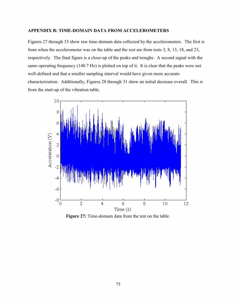
75

APPENDIX B: TIME-DOMAIN DATA FROM ACCELEROMETERS

Figures 27 through 33 show raw time-domain data collected by the accelerometers. The first is

from when the accelerometer was on the table and the rest are from tests 3, 8, 13, 18, and 23,

respectively. The final figure is a close-up of the peaks and troughs. A second signal with the

same operating frequency (140.7 Hz) is plotted on top of it. It is clear that the peaks were not

well-defined and that a smaller sampling interval would have given more accurate

characterization. Additionally, Figures 28 through 31 show an initial decrease overall. This is

from the start-up of the vibration table.

Figure 27: Time-domain data from the test on the table.

76

Figure 28: Time-domain data from Test 3.

Figure 29: Time-domain data from Test 8.

77

Figure 30: Time-domain data from Test 13.

Figure 31: Time-domain data from Test 18.

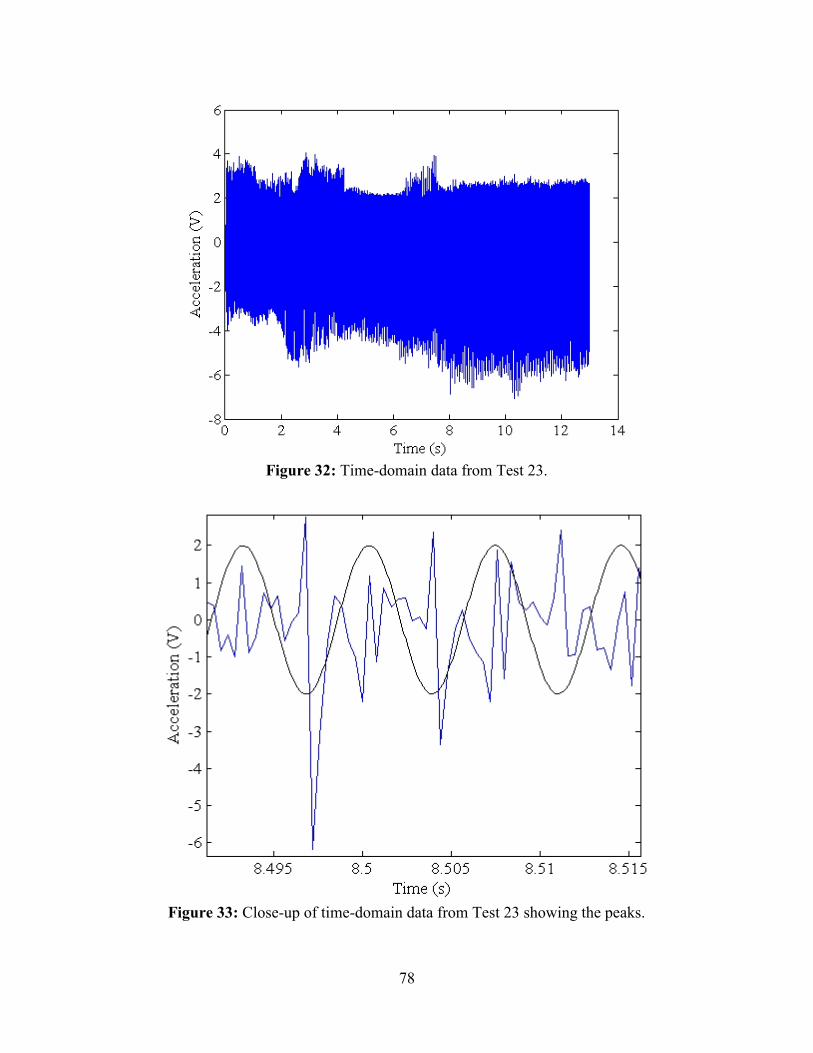
78

Figure 32: Time-domain data from Test 23.

Figure 33: Close-up of time-domain data from Test 23 showing the peaks.

79

APPENDIX C: MATLABTM CODES

The following are the MATLABTM codes that were used for analysis. The first is

MasterCurve.m, which was used to complete the power-law fitting. The second is

AccCodeV3.m, which was used to analyze the data from the accelerometers. The third is

DHR3.m, which was used to analyze the data from a DHR-3 rheometer by TA Instruments. The

use of the DHR-3 rheometer is discussed in Appendix D.

%MasterCurve.m: fits a power-law model to dataclear allclose allclc

%% Data%Mixture TEWte=[0.05 0.125 0.2 0.275]*2*pi;Tte=[9.83 13.59 16.07 17.03];

%Mixture N4Wn4=[0.5 0.425 0.275 0.2 0.125 0.05]*2*pi;Tn4=[14.52 14.71 12.08 11.81 10.53 7.74];

%Mixture H&N4Whn4=[0.275 0.2 0.125 0.05]*2*pi;Thn4=[18.56 16.71 14 8.09];

%Mixture TE&N4Wten4=[0.275 0.2 0.125 0.05]*2*pi;Tten4=[20.64 18.39 15.42 9.5];

%Mixture All67Wall=[0.2 0.125 0.05]*2*pi;Tall=[18.74 15.35 9.88];

%Strain ratesSR=linspace(0.01,10,1000);%% Parametersh=0.126; %mRo=0.3048/2-0.0127; %mRi=0.127/2; %m

%% Power Law model: T = H*WFitPL=@(param,Wdata,Tdata)(2*Wdata/(-param(1))*(2*pi*param(2)*h)^(1/param(1))/(Ro^(-2/param(1))-Ri^(-2/param(1)))).^param(1)-Tdata;

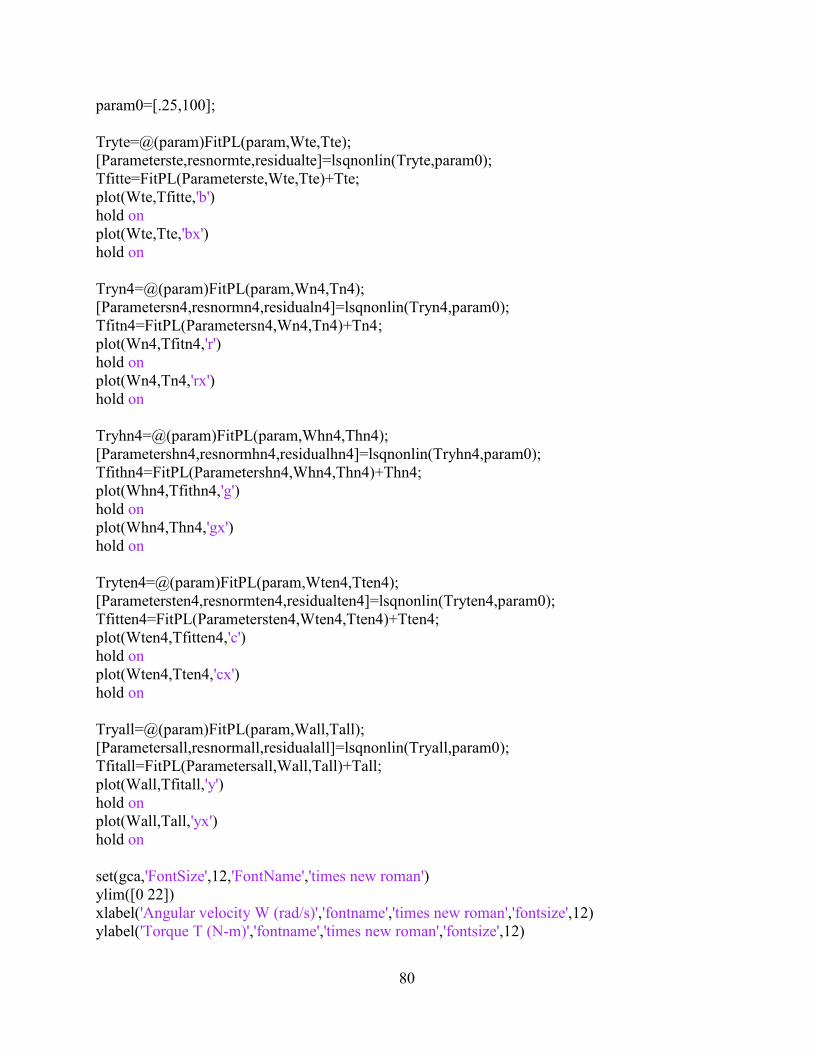
80

param0=[.25,100];

Tryte=@(param)FitPL(param,Wte,Tte);[Parameterste,resnormte,residualte]=lsqnonlin(Tryte,param0);Tfitte=FitPL(Parameterste,Wte,Tte)+Tte;plot(Wte,Tfitte,'b')hold onplot(Wte,Tte,'bx')hold on

Tryn4=@(param)FitPL(param,Wn4,Tn4);[Parametersn4,resnormn4,residualn4]=lsqnonlin(Tryn4,param0);Tfitn4=FitPL(Parametersn4,Wn4,Tn4)+Tn4;plot(Wn4,Tfitn4,'r')hold onplot(Wn4,Tn4,'rx')hold on

Tryhn4=@(param)FitPL(param,Whn4,Thn4);[Parametershn4,resnormhn4,residualhn4]=lsqnonlin(Tryhn4,param0);Tfithn4=FitPL(Parametershn4,Whn4,Thn4)+Thn4;plot(Whn4,Tfithn4,'g')hold onplot(Whn4,Thn4,'gx')hold on

Tryten4=@(param)FitPL(param,Wten4,Tten4);[Parametersten4,resnormten4,residualten4]=lsqnonlin(Tryten4,param0);Tfitten4=FitPL(Parametersten4,Wten4,Tten4)+Tten4;plot(Wten4,Tfitten4,'c')hold onplot(Wten4,Tten4,'cx')hold on

Tryall=@(param)FitPL(param,Wall,Tall);[Parametersall,resnormall,residualall]=lsqnonlin(Tryall,param0);Tfitall=FitPL(Parametersall,Wall,Tall)+Tall;plot(Wall,Tfitall,'y')hold onplot(Wall,Tall,'yx')hold on

set(gca,'FontSize',12,'FontName','times new roman')ylim([0 22])xlabel('Angular velocity W (rad/s)','fontname','times new roman','fontsize',12)ylabel('Torque T (N-m)','fontname','times new roman','fontsize',12)

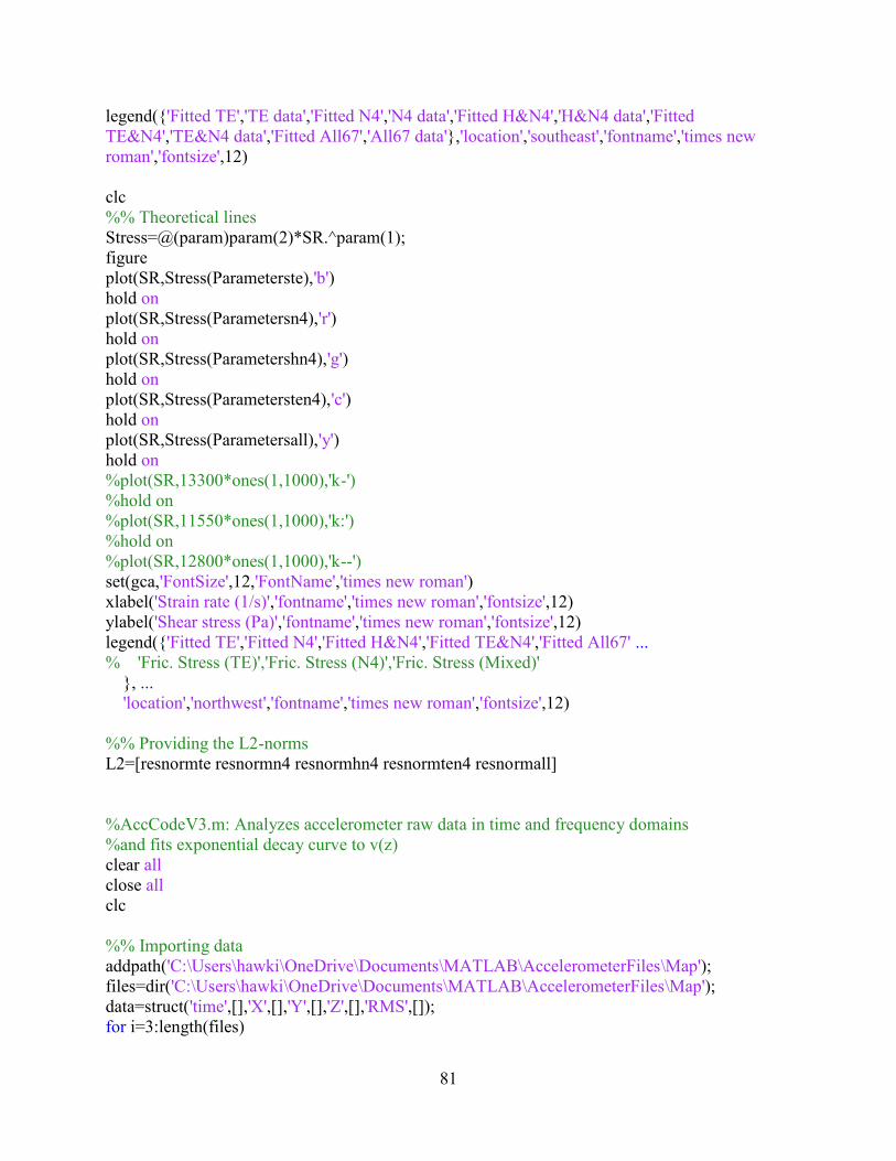
81

legend({'Fitted TE','TE data','Fitted N4','N4 data','Fitted H&N4','H&N4 data','FittedTE&N4','TE&N4 data','Fitted All67','All67 data'},'location','southeast','fontname','times newroman','fontsize',12)

clc%% Theoretical linesStress=@(param)param(2)*SR.^param(1);figureplot(SR,Stress(Parameterste),'b')hold onplot(SR,Stress(Parametersn4),'r')hold onplot(SR,Stress(Parametershn4),'g')hold onplot(SR,Stress(Parametersten4),'c')hold onplot(SR,Stress(Parametersall),'y')hold on%plot(SR,13300*ones(1,1000),'k-')%hold on%plot(SR,11550*ones(1,1000),'k:')%hold on%plot(SR,12800*ones(1,1000),'k--')set(gca,'FontSize',12,'FontName','times new roman')xlabel('Strain rate (1/s)','fontname','times new roman','fontsize',12)ylabel('Shear stress (Pa)','fontname','times new roman','fontsize',12)legend({'Fitted TE','Fitted N4','Fitted H&N4','Fitted TE&N4','Fitted All67' ...% 'Fric. Stress (TE)','Fric. Stress (N4)','Fric. Stress (Mixed)'

}, ...'location','northwest','fontname','times new roman','fontsize',12)

%% Providing the L2-normsL2=[resnormte resnormn4 resnormhn4 resnormten4 resnormall]

%AccCodeV3.m: Analyzes accelerometer raw data in time and frequency domains%and fits exponential decay curve to v(z)clear allclose allclc

%% Importing dataaddpath('C:\Users\hawki\OneDrive\Documents\MATLAB\AccelerometerFiles\Map');files=dir('C:\Users\hawki\OneDrive\Documents\MATLAB\AccelerometerFiles\Map');data=struct('time',[],'X',[],'Y',[],'Z',[],'RMS',[]);for i=3:length(files)

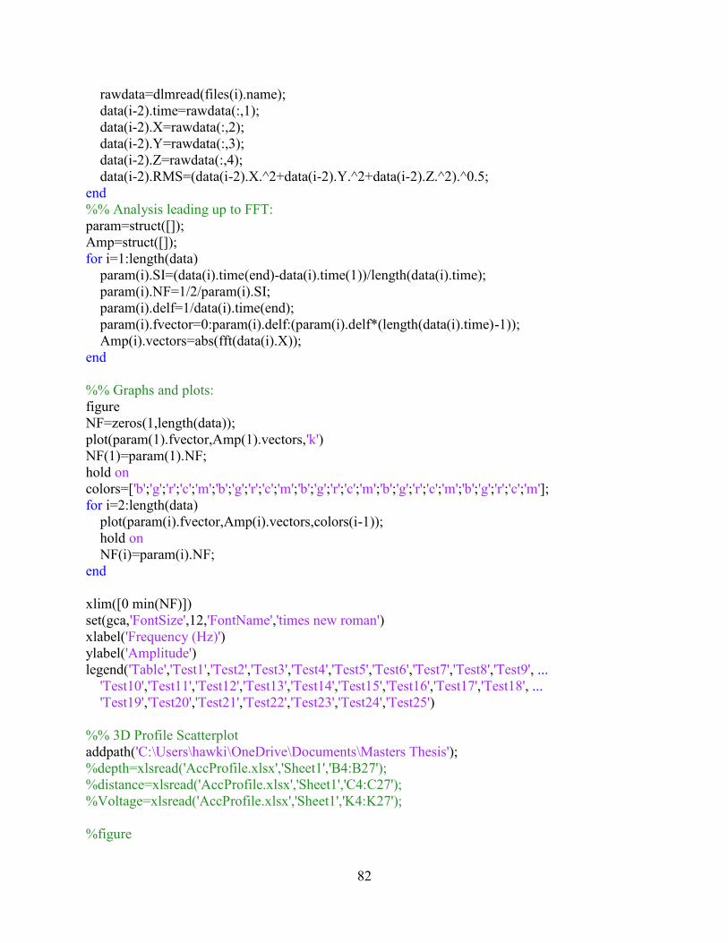
82

rawdata=dlmread(files(i).name);data(i-2).time=rawdata(:,1);data(i-2).X=rawdata(:,2);data(i-2).Y=rawdata(:,3);data(i-2).Z=rawdata(:,4);data(i-2).RMS=(data(i-2).X.^2+data(i-2).Y.^2+data(i-2).Z.^2).^0.5;

end%% Analysis leading up to FFT:param=struct([]);Amp=struct([]);for i=1:length(data)

param(i).SI=(data(i).time(end)-data(i).time(1))/length(data(i).time);param(i).NF=1/2/param(i).SI;param(i).delf=1/data(i).time(end);param(i).fvector=0:param(i).delf:(param(i).delf*(length(data(i).time)-1));Amp(i).vectors=abs(fft(data(i).X));

end

%% Graphs and plots:figureNF=zeros(1,length(data));plot(param(1).fvector,Amp(1).vectors,'k')NF(1)=param(1).NF;hold oncolors=['b';'g';'r';'c';'m';'b';'g';'r';'c';'m';'b';'g';'r';'c';'m';'b';'g';'r';'c';'m';'b';'g';'r';'c';'m'];for i=2:length(data)

plot(param(i).fvector,Amp(i).vectors,colors(i-1));hold onNF(i)=param(i).NF;

end

xlim([0 min(NF)])set(gca,'FontSize',12,'FontName','times new roman')xlabel('Frequency (Hz)')ylabel('Amplitude')legend('Table','Test1','Test2','Test3','Test4','Test5','Test6','Test7','Test8','Test9', ...

'Test10','Test11','Test12','Test13','Test14','Test15','Test16','Test17','Test18', ...'Test19','Test20','Test21','Test22','Test23','Test24','Test25')

%% 3D Profile Scatterplotaddpath('C:\Users\hawki\OneDrive\Documents\Masters Thesis');%depth=xlsread('AccProfile.xlsx','Sheet1','B4:B27');%distance=xlsread('AccProfile.xlsx','Sheet1','C4:C27');%Voltage=xlsread('AccProfile.xlsx','Sheet1','K4:K27');

%figure

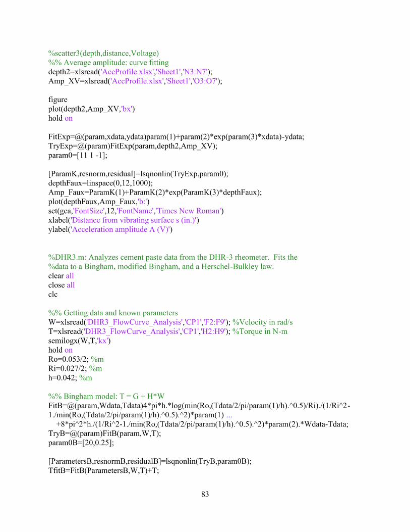
83

%scatter3(depth,distance,Voltage)%% Average amplitude: curve fittingdepth2=xlsread('AccProfile.xlsx','Sheet1','N3:N7');Amp_XV=xlsread('AccProfile.xlsx','Sheet1','O3:O7');

figureplot(depth2,Amp_XV,'bx')hold on

FitExp=@(param,xdata,ydata)param(1)+param(2)*exp(param(3)*xdata)-ydata;TryExp=@(param)FitExp(param,depth2,Amp_XV);param0=[11 1 -1];

[ParamK,resnorm,residual]=lsqnonlin(TryExp,param0);depthFaux=linspace(0,12,1000);Amp_Faux=ParamK(1)+ParamK(2)*exp(ParamK(3)*depthFaux);plot(depthFaux,Amp_Faux,'b:')set(gca,'FontSize',12,'FontName','Times New Roman')xlabel('Distance from vibrating surface s (in.)')ylabel('Acceleration amplitude A (V)')

%DHR3.m: Analyzes cement paste data from the DHR-3 rheometer. Fits the%data to a Bingham, modified Bingham, and a Herschel-Bulkley law.clear allclose allclc

%% Getting data and known parametersW=xlsread('DHR3_FlowCurve_Analysis','CP1','F2:F9'); %Velocity in rad/sT=xlsread('DHR3_FlowCurve_Analysis','CP1','H2:H9'); %Torque in N-msemilogx(W,T,'kx')hold onRo=0.053/2; %mRi=0.027/2; %mh=0.042; %m

%% Bingham model: T = G + H*WFitB=@(param,Wdata,Tdata)4*pi*h.*log(min(Ro,(Tdata/2/pi/param(1)/h).^0.5)/Ri)./(1/Ri^2-1./min(Ro,(Tdata/2/pi/param(1)/h).^0.5).^2)*param(1) ...

+8*pi^2*h./(1/Ri^2-1./min(Ro,(Tdata/2/pi/param(1)/h).^0.5).^2)*param(2).*Wdata-Tdata;TryB=@(param)FitB(param,W,T);param0B=[20,0.25];

[ParametersB,resnormB,residualB]=lsqnonlin(TryB,param0B);TfitB=FitB(ParametersB,W,T)+T;

84

semilogx(W,TfitB,'b:');

%% Modified Bingham model: T = G + H*W + C*W^2FitModB=@(param,Wdata,Tdata)4*pi*h.*log(min(Ro,(Tdata/2/pi/param(1)/h).^0.5)/Ri)./(1/Ri^2-1./min(Ro,(Tdata/2/pi/param(1)/h).^0.5).^2)*param(1) ...

+8*pi^2*h./(1/Ri^2-1./min(Ro,(Tdata/2/pi/param(1)/h).^0.5).^2)*param(2).*Wdata ...+8*pi^3*h./(1/Ri^2-

1./min(Ro,(Tdata/2/pi/param(1)/h).^0.5).^2).*(min(Ro,(Tdata/2/pi/param(1)/h).^0.5)+Ri)./(min(Ro,(Tdata/2/pi/param(1)/h).^0.5)-Ri)*param(3).*Wdata.^2 ...

-Tdata;TryModB=@(param)FitModB(param,W,T);param0ModB=[20 1 1];

[ParametersModB,resnormModB,residualModB]=lsqnonlin(TryModB,param0ModB);TfitModB=FitModB(ParametersModB,W,T)+T;semilogx(W,TfitModB,'r:');

%% Herschel-Bulkley model:FitHB=@(param,Wdata,Tdata)4*pi*h.*log(min(Ro,(Tdata/2/pi/param(1)/h).^0.5)/Ri)./(1/Ri^2-1./min(Ro,(Tdata/2/pi/param(1)/h).^0.5).^2)*param(1) ...

+2^(2*param(3)+1)*pi^(param(3)+1)*h*param(2)/param(3)^param(3)./(1/Ri^(2/param(3))-1./min(Ro,(Tdata/2/pi/param(1)/h).^0.5).^(1/param(3))).^param(3).*Wdata.^param(3) ...

-Tdata;TryHB=@(param)FitHB(param,W,T);param0HB=[20,1,1];

[ParametersHB,resnormHB,residualHB]=lsqnonlin(TryHB,param0HB);TfitHB=FitHB(ParametersHB,W,T)+T;semilogx(W,TfitHB,'g:');title('Fits for W-T data')xlabel('Angular velocity (rad/s)')ylabel('Torque (N-m)')legend('Data','Bingham','Modified Bingham','Herschel-Bulkley','location','northwest')

%% Residuals/error comparison:ZerosB=FitB(ParametersB,W,T);ZerosModB=FitModB(ParametersModB,W,T);ZerosHB=FitHB(ParametersHB,W,T);Resnorm=[resnormB,resnormModB,resnormHB]Rs=[min(Ro,(T/2/pi./ParametersB(1)/h).^0.5) min(Ro,(T/2/pi./ParametersModB(1)/h).^0.5)min(Ro,(T/2/pi./ParametersHB(1)/h).^0.5)]

figureplot(W,ZerosB,'b')hold onplot(W,ZerosModB,'r')

85

hold onplot(W,ZerosHB,'g')title('Absolute errors for each data point')xlabel('Angular velocity (rad/s)')ylabel('Error (N-m')legend('Bingham','Modified Bingham','Herschel-Bulkley')

clc%% NOTE about algorithm:%Options: Algorithm may be trust region reflective or Levenberg-Marquardt;%use optimset

86

APPENDIX D: THE PECLET NUMBER

Hanotin et. al. used the Peclet number to determine the tendency of the granular suspension to

flow. It is the lubrication stress divided by the frictional stress. In addition, they used the

frictional stress to define the boundary between two regimes. Because of the prominence of this

analysis in literature, it is worth including here even though the analysis needs some more

development. The first section discusses the frictional stress as a boundary between the two

regimes. The second section discusses the Peclet number.

D.1 Frictional Stress

The frictional stress was defined in Equation 23. The first variable is the coefficient of friction

between the grains, (not to be confused with the -parameter from the Bingham model). For

limestone, this is typically around 0.75 but different values have been reported so this is a source

of inaccuracy in the analysis46. The next variable is the difference between the density of the

grains and the density of the interstitial fluid. The specific gravity of the coarse aggregates

varies between each stock or size. For mixtures using multiple sizes, the average weighted by

volume fraction was taken. The density of the cement paste was measured at a hydration age of

30 minutes to be 1888 kg/m3. Because of particle migration and the added height required to

isolate the torque meter from the vibration table, the average depth of the measurement was

0.063 meters, the midpoint of the vane’s height. The gravitational constant is 9.81 m/s2 and the

coarse volume fraction was 0.67 for all of the mixtures except for TE, which had a fraction of

0.68. As discussed in Chapter 4, these fractions are overestimated due to particle settling. Table

10 summarizes these parameters and calculates the frictional stress for each mixture. Figure 34

plots the frictional stresses on the extrapolated power-law fits. On the one hand, there is good

agreement with data. A Newtonian regime exists, supporting the assumption of no yield stress in

the power-law fitting analysis. But it only occurs at such tiny shear rates that it cannot even be

seen. This reinforces the conclusion that the intermediary regime was more important for these

mixtures and under the applied vibration. On the other hand, the data above this frictional stress

does not follow the Bingham model at all.

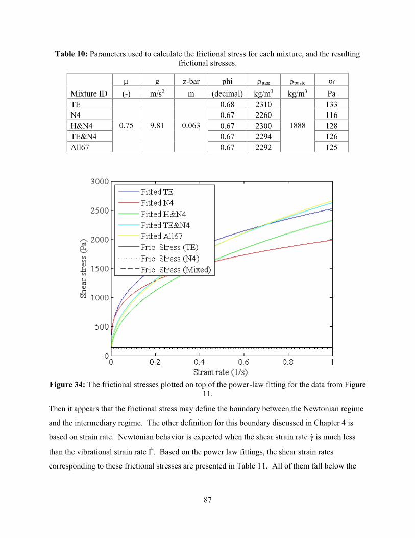
87

Table 10: Parameters used to calculate the frictional stress for each mixture, and the resultingfrictional stresses.

Mixture ID g z-bar phi agg paste σf

(-) m/s2 m (decimal) kg/m3 kg/m3 PaTE

0.75 9.81 0.063

0.68 2310

1888

133N4 0.67 2260 116H&N4 0.67 2300 128TE&N4 0.67 2294 126All67 0.67 2292 125

Figure 34: The frictional stresses plotted on top of the power-law fitting for the data from Figure11.

Then it appears that the frictional stress may define the boundary between the Newtonian regime

and the intermediary regime. The other definition for this boundary discussed in Chapter 4 is

based on strain rate. Newtonian behavior is expected when the shear strain rate is much less

than the vibrational strain rate . Based on the power law fittings, the shear strain rates

corresponding to these frictional stresses are presented in Table 11. All of them fall below the

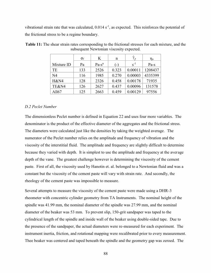
88

vibrational strain rate that was calculated, 0.014 s-1, as expected. This reinforces the potential of

the frictional stress to be a regime boundary.

Table 11: The shear strain rates corresponding to the frictional stresses for each mixture, and thesubsequent Newtonian viscosity expected.

Mixture IDσf K n ηo

Pa Pa-sn (-) s-1 Pa-sTE 133 2526 0.323 0.00011 1208437N4 116 1985 0.270 0.00003 4335399H&N4 128 2326 0.458 0.00178 71935TE&N4 126 2627 0.437 0.00096 131578All67 125 2663 0.459 0.00129 97556

D.2 Peclet Number

The dimensionless Peclet number is defined in Equation 22 and uses four more variables. The

denominator is the product of the effective diameter of the aggregates and the frictional stress.

The diameters were calculated just like the densities by taking the weighted average. The

numerator of the Peclet number relies on the amplitude and frequency of vibration and the

viscosity of the interstitial fluid. The amplitude and frequency are slightly difficult to determine

because they varied with depth. It is simplest to use the amplitude and frequency at the average

depth of the vane. The greatest challenge however is determining the viscosity of the cement

paste. First of all, the viscosity used by Hanotin et. al. belonged to a Newtonian fluid and was a

constant but the viscosity of the cement paste will vary with strain rate. And secondly, the

rheology of the cement paste was impossible to measure.

Several attempts to measure the viscosity of the cement paste were made using a DHR-3

rheometer with concentric cylinder geometry from TA Instruments. The nominal height of the

spindle was 41.99 mm, the nominal diameter of the spindle was 27.99 mm, and the nominal

diameter of the beaker was 53 mm. To prevent slip, 150-grit sandpaper was taped to the

cylindrical length of the spindle and inside wall of the beaker using double-sided tape. Due to

the presence of the sandpaper, the actual diameters were re-measured for each experiment. The

instrument inertia, friction, and rotational mapping were recalibrated prior to every measurement.

Thee beaker was centered and taped beneath the spindle and the geometry gap was zeroed. The

89

paste CP2 used in the mixtures from Table 4 was prepared as described in section 4.1.1. It was

then immediately poured into a 150-ml glass beaker that was used as the cup. The spindle was

lowered to a gap of 6 mm and a flow sweep test was conducted at a hydration age of 30 minutes.

The flow sweep test was strain-controlled and conducted from an angular velocity of 10 rad/s to

angular velocities of 0.01 rad/s or 0.001 rad/s. Four points were taken per decade, and each point

was collected once the material reached steady-state conditions. Because of the steady-state

requirement, no pre-shear period was required before the start of the test, which helped minimize

particle migration. The angular velocity and torque were recorded for analysis and the analyzed

using the MATLABTM code DHR3.m, provided in Appendix C.

The data from CP1 and CP2 are plotted in Figure 35. The legend identifies the mixtures by the

amount of silica fume replacement. Silica fume stiffens the mixture, making it more viscous, but

CP1 had greater torques than CP2. In addition, the CP2 data dips at about 2 rad/s. This indicates

that the mixture was slipping and this was indeed observed during the experiment at least for

CP2. It may have occurred for CP1 as well. Additionally, when these curves were fit to a

Herschel-Bulkley model, the model proclaimed them to be shear-thickening when it is well-

known that cement paste is a shear-thinning material.

Figure 35: (W , T) data for cement pastes CP1 and CP2 demonstrating slip.

Fortunately, the numerator of the Peclet number is the same for each of the concrete mixtures.

Then the denominator of the Peclet number may be considered in any analysis. The Peclet

number is supposed to be inversely proportional to the Newtonian viscosity ηo. Figure 36 plots

0

0.001

0.002

0.003

0.004

0.005

0.006

0.007

0.008

0.009

0.01

0.01 0.1 1 10 100

Torq

ue (N

-m)

Velocity (rad/s)

10% SF

5% SF

90

the Newtonian viscosity against the inverse of the denominator of the Peclet number. There is a

weak positive correlation but a linear relationship was expected. The cause of this discrepancy is

not known.

Figure 36: Plot of the Newtonian viscosity against the inverse of the denominator of the Pecletnumber.

0500

100015002000250030003500400045005000

0.5 0.7 0.9 1.1 1.3 1.5 1.7 1.9

η o(k

Pa-s

)

DPe-1 (Pa)

91

APPENDIX E: STRESS GROWTH TEST DATA FOR NON-VIBRATED, NO-SLUMPCONCRETES

Figures 37 through 40 provide the stress growth tests conducted on mixtures TE, N4, TE&N4,

and All67 during vibration at hydration ages of 30 minutes, respectively.

Figure 37: Stress growth test for TE.

Figure 38: Stress growth test for N4.

0

2000

4000

6000

8000

10000

12000

0 2 4 6 8 10 12

Stre

ss (P

a)

Time (s)

0

2000

4000

6000

8000

10000

12000

0 2 4 6 8 10

Stre

ss (P

a)

Time (s)

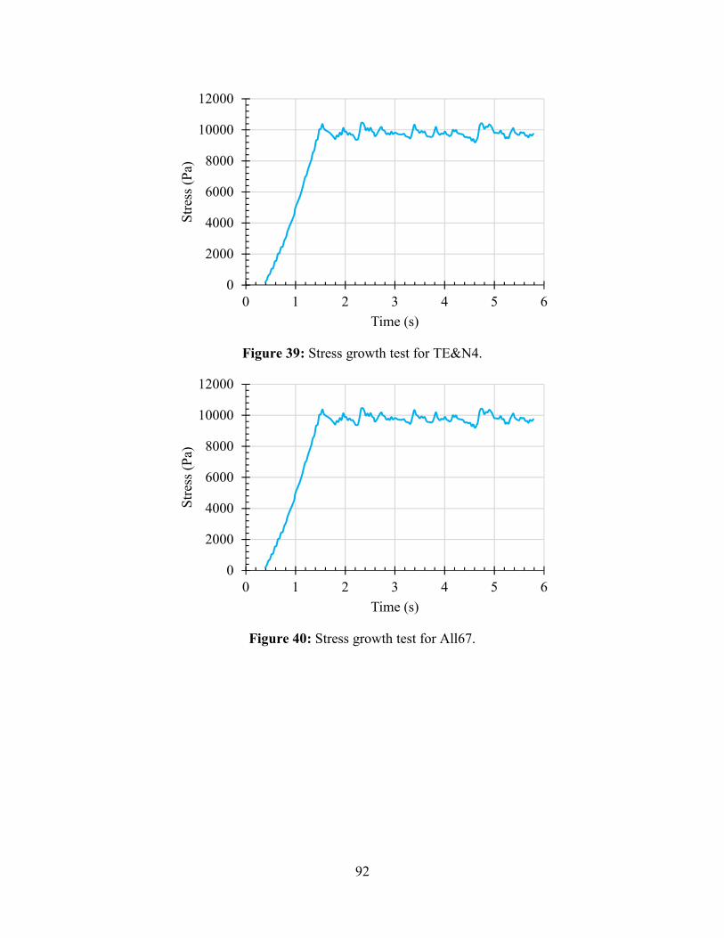
92

Figure 39: Stress growth test for TE&N4.

Figure 40: Stress growth test for All67.

0

2000

4000

6000

8000

10000

12000

0 1 2 3 4 5 6

Stre

ss (P

a)

Time (s)

0

2000

4000

6000

8000

10000

12000

0 1 2 3 4 5 6

Stre

ss (P

a)

Time (s)