ISTITUTO DI ANALISI DEI SISTEMI ED INFORMATICA

CONSIGLIO NAZIONALE DELLE RICERCHE

P. Augerat, J.M. Belenguer, E. Benavent,

A. Corberan, D. Naddef, G. Rinaldi

COMPUTATIONAL RESULTS

WITH A BRANCH-AND-CUT CODE

FOR THE CAPACITATED

VEHICLE ROUTING PROBLEM

R. 495 Dicembre 1998

Philippe Augerat, Denis Naddef – LMC-IMAG, Institut National Polytechnique de Greno-ble - B.P. 53, 38041 Grenoble Cedex 9, France.

Jose Manuel Belenguer, Enrique Benavent, Angel Corberan – Universitat de Valencia.Valencia, Spain.

Giovanni Rinaldi – Istituto di Analisi dei Sistemi ed Informatica del CNR, Viale Manzoni30, 00185 Roma.

This work was partially financed by the EEC Science Program SC1-CT91-620 and by the project CE92-

0007 of the Spanish Ministerio de Educacion y Ciencia.

Istituto di Analisi dei Sistemi ed Informatica, CNRviale Manzoni 3000185 ROMA, Italy

tel. ++39-06-77161fax ++39-06-7716461email: iasi@iasi.rm.cnr.itURL: http://www.iasi.rm.cnr.it

Abstract

In this paper, we present a branch-and-cut algorithm to solve the Capacitated Vehicle RoutingProblem (CVRP) to optimality, which is based on the partial polyhedral description of the cor-responding polytope. The valid inequalities used in the algorithm are proposed and described inCornuejols and Harche (1993), De Vitis, Harche, and Rinaldi (1999), and in Naddef and Rinaldi(1999) where also unpublished inequalities of Augerat and Pochet can be found. We concen-trated mainly on the design of separation procedures for several classes of valid inequalities.

The capacity constraints (generalized subtour elimination inequalities) happen to play a crucialrole in the development of a cutting plane algorithm for the CVRP. A number of separationheuristics have been implemented and compared for these inequalities. We also implementedheuristic separation algorithms for other classes of valid inequalities that also lead to significantimprovements: comb, capacity strengthened comb, and generalized capacity inequalities.

The resulting cutting plane algorithm has been applied to a set of instances taken from theliterature. The lower bounds obtained are better than the ones previously known. Some branch-ing strategies have been implemented to develop a branch-and-cut algorithm that has been ableto solve large CVRP instances, some of them that were still unsolved. The main results is thesolution of two versions of a 134-customer instance proposed by Fisher. These instances are, tothe best of our knowledge, the largest in the literature for which an optimal certified solutionhas been provided by an automatic procedure.

Key words: Capacitated Vehicle Routing Problem, branch-and-cut, valid inequalities.

AMS subject classifications: 05C35, 68E10,

3.

1. Introduction

The Capacitated Vehicle Routing Problem (CVRP) we consider in this paper consists in anoptimization that deals with the distribution of a commodity from a single depot to a given setof n customers with known demand, using a given number k of vehicles having all the samecapacity C. Each customer i must be served by exactly one vehicle, i.e., demand splitting isnot allowed, therefore the corresponding demand di must be entirely satisfied using exactly onevehicle. The total demand assigned to each vehicle must satisfy the capacity constraint, thusit cannot exceed C. Clearly the problem is feasible if the demand of each customer does notexceed C. The objective is to minimize the total distance traveled by the k vehicles. So, onceall customers have been assigned to the vehicles, one has to determine, for each vehicle, theminimum length route leaving the depot, visiting all customers assigned to it, and going backto the depot. In this paper, we only consider symmetric distances in the objective function.

There are many practical applications of CVRP in the public sector such as in school busrouting, pick up, and mail delivery, as well as in the private sector such as in the dispatching ofdelivery trucks. We refer to Bodin et al. [8], Christofides [11], Magnanti [28], Osman [36], andToth and Vigo [42] for a survey of vehicle routing applications, model extensions, and solutionmethods.

If the capacity C is large enough (at least∑n

i=1 di), then all possible assignments of customersto vehicles are feasible and the capacity constraints are redundant. In this case, the CVRPreduces to the multi-salesman problem (k-TSP). On the other hand, if the capacity C is smallcompared with the sum of the demands, the capacity limitation becomes a crucial part of theproblem that essentially amounts to requiring the solution of a bin packing problem for theassignment of the customers (or items of weight di) to the vehicles (or bins of size C). Sincek-TSP and bin packing are both NP-hard problems, CVRP being a combination of the two, isalso NP-hard. This is the reason why routing problems have first been tackled using heuristicapproaches. See again the above mentioned references and, for recent results, Hiquebrau etal. [22], Taillard [41], Osman [37], Gendreau et al. [20], and Campos and Mota [10].

During the past fifteen years, exact algorithms have also been developed to solve capacitatedrouting problems of reasonable size to optimality. Note that here and in the following by solvingan instance we mean providing one its optimal solution along with a certificate of optimality.For example, Agarwal et al. [1], Mingozzi et al. [31] use a set partitioning and column generationapproach and Fisher [19] uses a Lagrangean approach based on the minimum k-tree relaxation.Other exact approaches are presented in the surveys of Christofides [11] and Laporte [25].

Another way to solve CVRP instances is by using the polyhedral approach, which was shownto be efficient to solve large instances of a similar optimization problem, the traveling salesmanproblem (TSP).

Note that, the notion of “large instance” for CVRP is not quite the same as for TSP. Thisnotion is substantially related to the size of an instance is reasonable to expect to be solvableby an automatic procedure with the current mathematical methods and the current technologyin a practical amount of time, say one day of cpu time. Therefore, while a “large” TSP instancemay have thousands of nodes, what we consider today a “large” instance for CVRP has aboutone hundred customers. Fisher [19] reports on the solution of some test problems with up to100 customers to optimality, using a Lagrangean relaxation approach embedded in a branch-and-bound scheme. Actually, when we began this study the CVRP instance solved by Fisherwas the largest know in the literature that an algorithm was able to solve (in the above specifiedmeaning). On the other hand, some well known test problems with 76 customers still resist to

4.

be solved.Initial investigations on the polyhedral aspects of CVRP with customers having all the same

demand (identical customers) and on the similarities between the TSP and CVRP polyhedrawere conducted by Araque [3], Campos et al. [9], Araque et al. [4], Laporte and Nobert [26]and Laporte et al. [27]. A more complete description of the CVRP polyhedron can be foundin Cornuejols and Harche [15] and in Naddef and Rinaldi [32] in which unpublished results ofAugerat and Pochet are reported. Computational results using the polyhedral approach arereported in Araque et al. [5] (for the case of identical customers), Cornuejols and Harche [15],and Laporte et al. [27]. They solved moderate sized problems with up to 60 customers tooptimality.

In this paper we describe a branch-and-cut algorithm that we devised using the above resultson the polytope associated with CVRP, and we report on computational results. With thisalgorithm we were able to solve all the instances for which an optimal solution was alreadyreported in the literature as well as some still unsolved ones. The main results is the solutionof a 134-customer instance purposed by Fisher [19]. We solved two versions of this instanceobtained by taking different numbers of digits in the computation of the distance function.These two instances are, to the best of our knowledge, the largest in the literature for which anoptimal certified solution has been provided by an automatic procedure.

The content of the paper is as follows. In Section 2, we formally describe the CVRP andthe valid inequalities that we use in our branch-and-cut algorithm. In Section 3, we presentseparation procedures for the capacity constraints (generalized subtour elimination inequalities).In Section 4, we describe separation procedures for other valid inequalities and we show howthese procedures lead to significant improvements in the algorithm for some instances. Section 5is dedicated to the branching strategies. Finally, in Section 6 we report on some computationalresults for a set of difficult instances taken from the literature.

2. Problem description and known classes of valid inequalities

In this section we present the basic CVRP formulation and notation that are used in the follow-ing. The formulation we use is the so-called two index flow model whose main advantage residesin the small number of variables needed. We also briefly present most of the known classes ofvalid inequalities for this formulation.

2.1. Problem description

Let G(V,E) be an undirected complete graph with node set V containing n+1 nodes numbered0, 1, . . . , n. The distinguished node 0 corresponds to the depot and the other nodes correspondto the n customers. The set of customers is denoted by V0, so V = V0∪0. With each customeri ∈ V0, we associate a positive demand di. For each edge e ∈ E, we are given a positive costbe, which corresponds to the distance between the two end-nodes of e (cost of traveling alongthe edge e). Let k be the fixed number of vehicles available at the depot and C their commoncapacity.

For a given subset F of edges of E, G(F ) denotes the subgraph (V (F ), F ) induced by F ,where V (F ) is the set of nodes incident with at least one edge of F .

A route is either two copies of the same edge incident with the depot or a nonempty subsetF of E inducing a subgraph G(F ) that is a simple cycle containing the depot 0 (i.e., 0 ∈ V (F ),G(F ) is connected, and the degree of each node of V (F ) in G(F ) is 2) and such that the total

5.

demand of nodes (customers) in V0(F ) = V (F ) \ 0 does not exceed the vehicle capacity C.Such a route represents the trip of one vehicle leaving the depot, satisfying the demand of thenodes in V0(F ) (traveling along the edges F ), and going back to the depot. The length of a routeis the sum of the traveling costs be over all the edges e ∈ F . Note that if |V (F )| = 2 in a route F ,then the route is composed by twice the same edge. In all the other cases (i.e., |V (F )| > 2), anedge can appear only once in a route. Note that in the literature some authors do not acceptthe case of a route visiting a unique customer. On the other hand, most of the problems of theliterature are “tight”, that is the minimum number of vehicles needed to serve V \ v is also kfor all v, and therefore the case of such “degenerate” routes is rare. As a matter of fact, in ourcomputational experiments none of the optimal solutions that we obtained has such degenerateroutes, therefore these solutions remain optimal also if these routes are explicitly forbidden.

A k-route is defined as a subset R of E that can be partitioned into k routes R1, R2, . . . , Rk

and such that each node i ∈ V0 belongs to exactly one of the k routes (i.e., to exactly one ofthe sets V (Rj), 1 ≤ j ≤ k). The length of a k-route is the sum of the lengths of the k differentroutes composing it. Each k-route defines a feasible solution to CVRP and the optimizationproblem consists in finding a minimum length k-route.

2.2. Notation

In order to formulate the CVRP as an integer program, with each k-route we associate anincidence vector χ ∈ R

E, i.e., a |E|-dimensional vector with components indexed by the elementsof E such that the component xe associated to edge e represents the number of times e is usedby the k-route. Sometimes, we will write xij instead of xe, where e is the edge with endnodes iand j, i < j. Let us denote by XCV RP the set of all feasible k-route of the problem. Then theCVRP polytope is the convex hull of the incidence vectors of all the elements of XCV RP .

Let S be a subset of V . Then the set δ(S) (called coboundary of S) is the set of the edgeswith one endnode in S and the other in V \ S, i.e., δ(S) = (i, j) ∈ E | i ∈ S, j ∈ V \ S. Inaddition, if S′ is a subset of V \S, the set (S : S′) (cut between S and S′) is the set of the edgeswith one end-node in S and the other in S′, i.e., (S : S′) = (i, j) ∈ E | i ∈ S, j ∈ S′. The setγ(S) is the set of edges with both endnodes in S, i.e., γ(S) = (i, j) ∈ E | i, j ∈ S. By d(S) wedenote the total demand of the nodes in the set S, i.e., d(S) =

∑

i∈S di. Finally, if x ∈ RE, for

any subset F of E by x(F ) we denote the sum of the xe for all the edges e in F .

2.3. CVRP formulation

Now we can now formulate the CVRP as the following integer program:

(CVRP) min∑

e∈E bexe (1)

x(δ(0)) = 2k (2)

x(δ(i)) = 2 for all i ∈ V0 (3)

x(δ(S)) ≥ 2⌈

d(S)C

⌉

for all S ⊆ V0, S 6= ∅ (4)

0 ≤ xe ≤ 1 for all e ∈ γ(V0) (5)

0 ≤ xe ≤ 2 for all e ∈ δ(0) (6)

xe integer for all e ∈ E. (7)

Constraint (2) states that each of the k vehicles has to leave from and go back to the depot.Constraints (3) are the degree constraints at each customer node. Constraints (4) are the

6.

capacity constraints (also called generalized subtour elimination constraints), where ⌈α⌉ standsfor the smallest integer greater than or equal to α. They mean that, for a given subset S ofcustomers, at least ⌈d(S)/C⌉ vehicles are needed to satisfy the demand in S and, because thedepot is outside S, the route corresponding with each of these vehicles must necessarily enter andleave the set S. Furthermore, like for the subtour elimination constraints in the case of the TSP,these constraints are needed to force the connectivity of the solution. Constraints (5)–(7) specifythe integrality and the bound restrictions on the variables. A variable xe linking a customernode directly to the depot (in (6)) can take the value 2 when a route serves only this customer,so this edge is traveled twice by the route. It is not difficult to check that the only solutions to(2)–(7)) are the incidence vectors of all the elements of XCV RP , thus (2)–(7)) is an integer linearprogramming formulation of CVRP. The constraints (2)–(6)) define a polytope that properlycontains the CVRP polytope and thus provide a linear programming (LP) relaxation to theproblem. Such a relaxation can be exploited in a branch-and-cut algorithm to provide a lowerbound to the optimal value. Such a bound may not be strong enough to reach the optimalsolution efficiently. Therefore it may be necessary to strengthen this formulation with othervalid inequalities.

Since this LP relaxation and its strengthened versions have an exponential number of con-strains, to optimize over such relaxations, in order to compute the lower bound, we have im-plemented a LP based cutting plane algorithm which proceeds in the following way. At eachiteration, a linear program including the degree constraints and some (polynomially sized) set ofvalid inequalities is solved. If the optimal LP solution corresponds to a k-route, we are done: theLP solution is the incidence vector of an optimal k-route. Otherwise, we strengthen the linearprogram by adding a set of valid inequalities violated by this optimal solution, and proceed asbefore. This cutting plane algorithm has been integrated in a branch-and-cut scheme to solvethe CVRP.

We now briefly present the classes of valid inequalities for XCV RP that we use in our cuttingplane algorithm and, in the next section, we will present the separation procedures that wehave implemented to find valid inequalities from these classes that are violated by a given LPsolution.

2.4. Capacity constraints

Denote by R(S) the minimum number of vehicles needed to satisfy the customers demand in aset S in any feasible solution. Note that from this definition it follows that the solution r(S)of a bin packing instance, where the bins have capacity C and the items are the element of Swith weights given by the vector d, is a lower bound for R(S). Actually it is possible that if weimpose that the set S be served by r(S) vehicles, then it is not possible to serve all clients withk vehicles. We obtain the following valid inequality

x(δ(S)) ≥ 2R(S) for all S ⊆ V0, S 6= ∅ (8)

It is NP-hard to compute R(S) but the inequality remains valid if R(S) is replaced by anylower bound of R(S). We chose to use the inequality (4) instead of (8) because computing R(S)appeared to be quite expensive. By the way for almost all the instances we considered in ourcomputational experiments the computation the exact value R(S) would have not produced anyeffect in the resulting relaxation.

7.

S1

S3

S2

S4

S5

S6

550

150150

150

100

300

150

450

125 950

100

150

300

1500

100

3100 200

100

125300

400150

300

500

800

1000

100150

3001

1/2

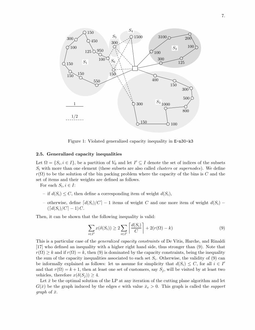
Figure 1: Violated generalized capacity inequality in E-n30-k3

2.5. Generalized capacity inequalities

Let Ω = Si, i ∈ I, be a partition of V0 and let I ′ ⊆ I denote the set of indices of the subsetsSi with more than one element (these subsets are also called clusters or supernodes). We definer(Ω) to be the solution of the bin packing problem where the capacity of the bins is C and theset of items and their weights are defined as follows.

For each Si, i ∈ I:

– if d(Si) ≤ C, then define a corresponding item of weight d(Si),

– otherwise, define ⌈d(Si)/C⌉ − 1 items of weight C and one more item of weight d(Si) −(⌈d(Si)/C⌉ − 1)C.

Then, it can be shown that the following inequality is valid:

∑

i∈I′

x(δ(Si)) ≥ 2∑

i∈I′

⌈

d(Si)

C

⌉

+ 2(r(Ω) − k) (9)

This is a particular case of the generalized capacity constraints of De Vitis, Harche, and Rinaldi[17] who defined an inequality with a higher right hand side, thus stronger than (9). Note thatr(Ω) ≥ k and if r(Ω) = k, then (9) is dominated by the capacity constraints, being the inequalitythe sum of the capacity inequalities associated to each set Si. Otherwise, the validity of (9) canbe informally explained as follows: let us assume for simplicity that d(Si) ≤ C, for all i ∈ I ′

and that r(Ω) = k + 1, then at least one set of customers, say Sj, will be visited by at least twovehicles, therefore x(δ(Sj)) ≥ 4.

Let x be the optimal solution of the LP at any iteration of the cutting plane algorithm and letG(x) be the graph induced by the edges e with value xe > 0. This graph is called the supportgraph of x.

8.

Figure 1 corresponds to the support graph associated with a fractional solution. The edgesrepresented by dotted lines have value 0.5, the solid lines are edges with value 1. The depotis represented by a square and the demands are written next to each node. Further data areC = 4500 and k = 3. For all the sets Si, i = 1, . . . , 6 the value of the coboundary is 2. Yetthe bin packing problem with bins having capacity 4 500 and 6 items having size d(S1) = 3 175,d(S2) = 3 925, d(S3) = 3 700, d(S4) = 1 500, d(S5) = 300, and d(S6) = 150, gives a value of 4while only 3 vehicles are available. Therefore, the inequality

∑3i=1 x(δ(Si)) ≥ 8 is violated by

the solution of Figure 1.When the same idea is applied to a partition of a subset H of V0, we have a framed inequality

introduced by Augerat and Pochet [7] (see also Naddef and Rinaldi [32]). Let H be a subsetV0, ΩH = Si, i ∈ I be a partition of H, and let I ′ and the weight of each item be defined asabove. If r(ΩH) is the solution of the bin-packing problem on ΩH , we have the bin inequality

x(δ(H)) +∑

i∈I′

x(δ(Si)) ≥ 2∑

i∈I′

⌈

d(Si)

C

⌉

+ 2r(ΩH). (10)

In Figure 1, let H = V0 \S2, and consider the partition made of the same sets as above except S2

(the shaded set). Then the corresponding framed inequality is violated. Indeed, the inequality“says” that if only two vehicles serve the customers of H, as it is currently the case in theexample since x(δ(H) = 4, then S1 and S3 cannot each be served by a single vehicle, as it isagain the case since x(δ(S1) = x(δ(S2) = 2, because then there would be no ways to pick upthe customer of demand 1 500. Consequently, either 3 vehicles serve H or at least 2 vehicles areused to serve one of two sets S1 and S3.

2.6. Comb inequalities and other TSP valid inequalities

In [32], Naddef and Rinaldi show that all valid inequalities for the traveling salesman polytopewhen written in tight triangular form are also valid for the CVRP polytope. This is in particulartrue for the well known comb inequalities.

Let Ti, i = 1, . . . , t (the teeth) and H (the handle) be subsets of V satisfying:

(i) Ti \ H 6= ∅, i = 1, . . . , t

(ii) Ti ∩ H 6= ∅, i = 1, . . . , t

(iii) Ti ∩ Tj = ∅, i = 1, . . . , t, j = 1, . . . , t, i 6= j

(iv) t is odd.

The corresponding comb inequality in tight triangular form is

x(δ(H)) +t

∑

i=1

x(δ(Ti)) ≥ 3t + 1 (11)

Note that the inequality (11) does not change if any node set in (11) is replaced by its comple-ment; on the other hand, complementing a tooth would violate some of the conditions that thefamily of sets that defines a comb inequality must satisfy. A property that teeth and handlemust satisfy when any of them are replaced by their complements is that the handle and itscomplement must have nonempty intersection with each tooth. The condition that qualifies a

9.

family of sets to be the teeth of a comb becomes quite weird if arbitrary complementation of theteeth is allowed. To simplify the matter, in particular for separating the comb inequalities, weallow only two possibilities: either the teeth are pairwise disjoint (and this is the case describedby the conditions (i)-(iv) above) or they are pairwise disjoint except for one tooth that mustcontain all the others.

Doing so, we can assume that the depot is in neither the handle nor in a tooth. This remarksimplifies the separation procedures for combs significantly.

As noted and explained in Naddef and Rinaldi [32], unfortunately most of the comb inequalitiesare not even binding for the CVRP polytope. This is due to the demands of the nodes and tothe capacity requirements that may make no feasible CVRP solution satisfy a comb inequalityat equality.

3. Separation of capacity constraints

De Vitis, Queyranne, and Rinaldi [18] showed that the problem of finding a capacity con-straints (4) violated by x by more than ǫ is polynomially solvable for a fixed ǫ. They alsoshowed that the separation of a stronger version of the capacity inequalities, obtained by tak-ing r(S) as a right hand side, is NP-hard. The procedure described in [18] is computationallyquite expensive, therefore we decided to use some heuristics implementing the following ideasproposed by Harche and Rinaldi [21]:

1. If G(x) is not connected, then the node set of each connected component not containingthe depot defines a violated capacity constraint. Therefeore from now on we assume thatG(x) is connected.

2. The node set of each connected component of the graph G(x) \ 0 is a candidate fordefining a violated capacity inequality. A check can be easily performed for each such set.

3. Recursively, shrink each edge e with value xe ≥ 1 and non incident with the depot (seePadberg and Rinaldi [39] for a detailed description of the shrinking procedure in the TSPcontext). Shrinking an edge e means removing it from the graph and contracting the twoendpoints of e into a supernode with demand equal to the sum of their demands. If thesupernode has a demand greater than C, the set of vertices in the supernode violates (4).Let G⋆(x) be the shrunk graph thus obtained. It can be easily shown that finding aviolated capacity constraint on G(x) is equivalent to finding it on G⋆(x). So, from now on,the heuristics in this section will be executed on G⋆(x) that, for notational convenience,we will be renamed G(x).

3. Fractional capacity inequalities are obtained by replacing⌈

d(S)C

⌉

in (4) by d(S)C

. Let f(S) =

x(δ(S)) − 2d(S)C

. It is possible to find the set S ⊆ V0 for which f(S) is minimum by usinga max-flow based polynomial time algorithm proposed by McCormick, Rao, and Rinaldi[30]. If f(S) < 0, then the fractional capacity inequality as well as the correspondingconstraint (4) are violated. If f(S) ≥ 2 all the inequalities (4) are satisfied. If 0 ≤ f(S) ≤ 2the capacity inequality defined by S is a good candidate and has to be checked explicitlyfor violation.

We have implemented all these procedures together with some additional simple ideas that canalso be used with other procedures too. Once a set S has been checked for producing a violated

10.

inequality (4), it is an easy task to do the same for set V0 \ S. Furthermore, sets with demandexceeding an integer multiple of C, are good candidates to produce a violated inequality (4).Then, every time a set S for which pC ≥ d(S) ≥ (p− ǫ)C, with p integer and ǫ = 0.33, is found,then (4) is checked for all the sets S ∪ v where v is adjacent to at least one node of S.

The results obtained with the Harche-Rinaldi procedures, including the above simple enhance-ments, are presented in Table 1.

3.1. Greedy shrinking algorithm

Another heuristic procedure for finding violated capacity inequalities is the following, which isalso known as the max-back growing of a set.

Given an initial set of nodes S, at each iteration of this procedure, the node v⋆, that maximizesx(δ(S : v)) over all v /∈ S, is added to S. The idea behind this choice is that the chosen node isthe one that added to S yields a set with the smallest coboundary among those that contain Sand differ from it by a single node. Of course after a few iterations, the obtained set may nothave a minimal coboundary among all sets that differ from the starting set by the same numberof nodes. Nevertheless it is a good heuristic which can be turned into an exact algorithm asshown by Nagamochi and Ibaraki ([35]).

This turns into a heuristic search for violated capacity inequalities. At each iteration theinequality (4) defined by S, and its stronger version with r(S) as a right hand side, is checkedfor possible violation.

Possible candidates for the starting node set S are:

1) a single node,

2) the end-points of an edge,

3) a set corresponding to a capacity inequality satisfied with equality by the current optimalLP solution,

4) the complement of such a set in V ,

5) any set including the depot,

6) any set not including the depot.

The number of initial sets according to the strategies from 1 to 4 is fixed. In the otherstrategies, we generate node sets randomly. In particular, we consider 10n randomly generatedinitial sets.

The best results were obtained for Strategy 6 and were improved by mixing it with Strategy 1(which is the fastest one). Computational results for the greedy shrinking algorithm are shownin Table 1.

Procedures similar to those described above were developed independently by Araque et al. [5]for the CVRP with identical customers.

3.2. Tabu search algorithm

The greedy shrinking algorithm can be generalized by allowing the current set S to be modified,not only by adding a new node to it, but also by removing a node already in S. In this way,the search for a set S violating the capacity constraint is considerably expanded, although the

11.

Table 1

Name Upper Bound LB HR LB max-back LB Tabu

E-n101-k8 817 788.76 795.08 796.15E-n22-k4 375 375 375 375E-n23-k3 569 569 569 569E-n30-k3 534 508.5 508.5 508.5E-n33-k4 835 831.1 833.2 833.5E-n51-k5 521 510.9 514.5 2 514.52E-n76-k10 832 773.60 787.47 789.31E-n76-k7 683 659.47 660.83 661.25E-n76-k8 735 703.48 709.68 711.05F-n135-k7 1165 1154.2 1155.89 1157.55F-n45-k4 724 723.8 724 724F-n72-k4 238 232.5 232.5 232.5M-n101-k10 820 818.16 819.33 819.33

Table 2

LB HR LB max-back LB Tabu

average gap 2.22 1.86 1.81maximum gap 4.8 4.8 4.8number of wins 4 7 11average number of cuts 339 946 2299average number iterations 50 33.5 31.2average cpu time 171 182 859

possibility of cycling arises. A simple tabu search procedure has been implemented using theseideas. We refer the reader to [6] for a detailed description of the procedure.

The tables compare the results obtained by the cutting plane algorithm when different heuris-tics are used to identify violated capacity constraints. The heuristics we compare are: thoseexplained at the beginning of this section which are due, mainly, to Harche and Rinaldi [21] (de-noted HR in the tables), the greedy shrinking algorithms, and the tabu search. Table 1 showsthe lower bounds obtained using the different identification heuristics on a set of instances takenfrom the literature. The problem instances that we use for this and for the following tables willbe referred to by a string X-nxx-ky, where xx is the number of nodes, i.e., the number of cus-tomers plus 1, y is the number of vehicles, if X is equal to “E” the instance is from Christofidesand Eilon [12] and can be found in the TSPLIB (see Reinelt [40]) under the prefix eil, if itis equal to “F” the instance comes from Fisher [19], finally if it is equal to “M” the source isMingozzi et al. [31].

Details on these instances and on the upper bounds shown, will be given in Section 6. Table 2gives a statistical summary of these results. The term gap refers to the relative distance betweenthe upper and lower bounds in percentage.

The best results were obtained by combining the greedy shrinking algorithm and Tabu. Thestrategy used was to call Tabu only in those iterations where the greedy shrinking procedurefailed to find a violated inequality. The results thus obtained are shown in Table 3.

12.

Table 3

Upper Lower cpu cpu #Name Bound Bound Gap lp solver identification iterations

E-n101-k8 817 796.314 2.5 100.09 194.31 56E-n22-k4 375 375 0 1.06 1.07 22E-n23-k3 569 569 0 0.42 0.33 9E-n30-k3 534 508.5 4.8 2.17 1.2 21E-n33-k4 835 833.5 0.18 3.73 2.91 23E-n51-k5 521 514.524 1.2 8.01 8.58 25E-n76-k10 832 789.416 5.1 152.36 194.42 70E-n76-k7 683 661.256 3.2 51.14 95.79 42E-n76-k8 735 711.17 3.2 81.91 176.14 73F-n135-k7 1165 1158.25 0.58 1198.07 314.79 123F-n45-k4 724 724 0 5 2.78 27F-n72-k4 238 232.5 2.3 8.56 2.87 19M-n101-k10 820 819.5 0.061 138.1 42.26 46Average gap: 1.78 Average total cpu time: 214 Average number of iterations: 42.8

4. Separation of other inequalities

4.1. Generalized capacity constraints

We first describe procedures used to find a violated inequality (9).Let Ω be a partition of V0 consisting of sets of coboundary value 2 in G(x). The best starting

partition would be the one consisting of maximal such sets. Note that this partition can beobtained in polynomial time, since finding all sets of coboundary value equal to 2 can be donein polynomial time (see, e.g., De Vitis [16]). In the implementation reported here, the elementsof the initial partition with more than one node are given by the node sets of maximal pathsof edges of x-value 1. In Figure 1 the original partition is the one shown. The elements of thepartition with more than one node are called supernodes. We can assume that each such set isshrunk into a single node with demand equal to the sum of the demands of its nodes. Thereforein the following we do not distinguish between nodes and supernodes.

At each iteration two elements of the partition are merged creating a new supernode andyielding the new current partition Ω. The bin packing value on Ω is denoted by r(Ω) (seeSection 2.5). We only compute r(Ω) if there is a good chance of violation. For this purpose welet incre be a variable whose value is equal to the amount by which the constraint (9) definedby Ω would be violated in case r(Ω) = k + 1 would hold. If incre ≤ 0, then r(Ω) need not becomputed. In other words we keep track of the excess of the coboundary value of each set of thepartiton over the right hand side of the corresponding capacity constraints. If this total amountis at least 2, then a violation is very unlikely to occur, as it is very unlikely that r(Ω) > k + 1.

By d(u) we denote the demand of node (or of the supernode) u.

Procedure 1. (Global shrinking)

0. Let Ω be a partition into sets of coboundary 2 in G(x). Set incre = 2.

1. If incre > 0, compute r(Ω), otherwise go to step 2. If r(Ω) > k, then the constraint (9) isviolated and we stop.

13.

Table 4

Upper Lower cpu cpu #Name Bound Bound Gap LP solver identification iterations

E-n101-k8 817 796.314 2.5 120.69 263.71 56E-n22-k4 375 375 0 1.3 1.5 22E-n23-k3 569 569 0 0.63 0.5 9E-n30-k3 534 532.5 0.28 6.18 8.83 50E-n33-k4 835 833.5 0.18 4.36 4.08 23E-n51-k5 521 514.524 1.2 9.56 12.57 25E-n76-k10 832 789.416 5.1 175.98 254.56 70E-n76-k7 683 661.256 3.2 62.39 130.27 42E-n76-k8 735 711.17 3.2 99.6 232.48 73F-n135-k7 1165 1158.25 0.58 1424.33 391.8 123F-n45-k4 724 724 0 6.08 3.4 27F-n72-k4 238 235 1.3 36.15 109.33 101M-n101-k10 820 819.5 0.061 164.59 56.34 46Average gap: 1.36 Average total cpu time: 275 Average number of iterations: 51.3

2. Otherwise, select the two elements Si and Sj of Ω that maximize x(X : Y ), over all X andY in Ω.

3. Let y = x(Si : Sj). Set incre = incre + 2y − 2(⌈

d(Si)C

⌉

+⌈

d(Sj )C

⌉

−⌈

d(Si)+d(Sj )C

⌉

).

4) Let Ω = Ω\Si, Sj∪Si∪Sj. If |Ω| = 1, stop. Otherwise check for violation the capacityconstraint defined by the supernode just created and go to step 1.

Separating framed capacity constraints (10) seems much more important to improve the effi-ciency of the branch-and-cut algorithm, but also much more complex. As we have already seenin the example of Figure 1, if all the edges in G(x) of the coboundary of a subset Si ∈ Ω areincident with the depot, this subset can be removed from Ω and H can be set to V0 \ Si. Thisoperation is repeated until no more elements of Ω have such a property.

Table 4 shows the lower bounds obtained with the cutting plane algorithm that uses the greedyshrinking and Tabu algorithms for the identification of capacity constraints and all the aboveprocedures to identify generalized capacity constraints. A group of procedures is called onlywhen the previous ones have not found any violated inequality.

In our tests the separation procedures that we described for the generalized capacity con-straints are really useful only for two instances E-n30-k3 (see Figure 1), and F-n72-k4. Forboth of them the improvements are significant. This shows that this class of inequality is com-putationally effective but also that its usefulness depends on the kind of instance at hand. Theinstances E-n30-k3 and F-n72-k4 are special in the sense that some clients have very largedemands making the bin packing problem crucial. This fact explains why in general these in-equalities become more and more effective as we go deeper in the branch-and-cut tree, whensupernodes are created after fixing a variable to the value 1.

4.2. Combs

The classical comb separation procedure is based on the biconnected components of the graphG⋆ obtained from G(x) by deleting all edges with value 1. Each of these components is used in

14.

turn as a candidate handle H. The candidate teeth are the nodeset of the edges with value 1that intersect H in one node, and the other biconnected components that intersect H. We alsotry, as candidate set for a handle, the union of two intersecting biconnected components. Formore details see Padberg and Rinaldi [38].

Clochard and Naddef [14], have developed a very fast and efficient procedure in which acandidate handle H is grown by the max-back procedure previously described, starting at anode incident with an edge of value 1. At some specified steps of this process candidate teethare searched for. First the nodes of all edges incident to H of large x-value are used as teeth.Other candidate teeth are produced, also by a max-back procedure, starting with a node v of Hthat minimizes x(v : H \ v) and is not contained in any previously found tooth.

These procedures have been refined for many other classes of TSP inequalities by Naddef andThienel ([33], [34]).

The only difficulty with repsect to the TSP case is due the depot. As we have seen, bycomplementing sets we can assume the depot to be neither in the handle nor in a tooth. Thereforein some cases of the previously described heuristic, we also search for the last tooth startingwith a set containing all the previously found teeth.

As explained in detail by Naddef and Rinaldi in [32] comb inequalities are in general weakinequalities for the CVRP. Stronger inequalities can be found if the capacities constraints aretaken into account. The routines of Clochard and Naddef [14] and those of Naddef and Thienel([33], [34]), could easily be modified to take the capacity constraints into account. However, inthe current implementation of the algorithm with which we have produced the compuationalresults given here does not use such more elaborate routines.

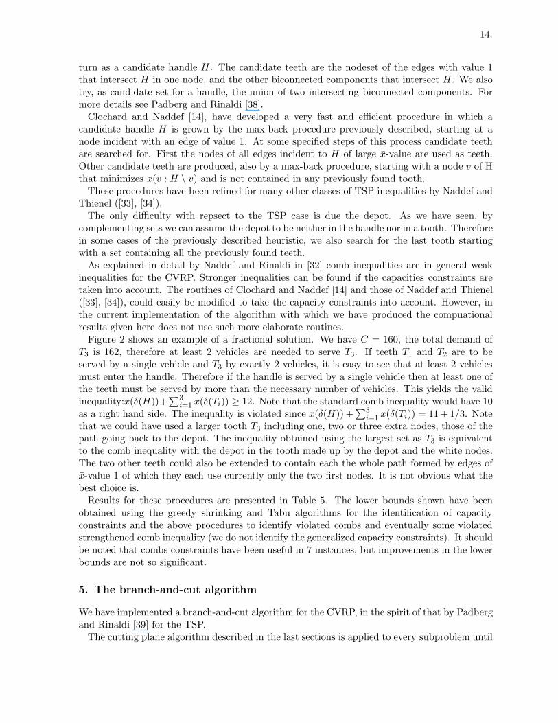
Figure 2 shows an example of a fractional solution. We have C = 160, the total demand ofT3 is 162, therefore at least 2 vehicles are needed to serve T3. If teeth T1 and T2 are to beserved by a single vehicle and T3 by exactly 2 vehicles, it is easy to see that at least 2 vehiclesmust enter the handle. Therefore if the handle is served by a single vehicle then at least one ofthe teeth must be served by more than the necessary number of vehicles. This yields the validinequality:x(δ(H))+

∑3i=1 x(δ(Ti)) ≥ 12. Note that the standard comb inequality would have 10

as a right hand side. The inequality is violated since x(δ(H)) +∑3

i=1 x(δ(Ti)) = 11 + 1/3. Notethat we could have used a larger tooth T3 including one, two or three extra nodes, those of thepath going back to the depot. The inequality obtained using the largest set as T3 is equivalentto the comb inequality with the depot in the tooth made up by the depot and the white nodes.The two other teeth could also be extended to contain each the whole path formed by edges ofx-value 1 of which they each use currently only the two first nodes. It is not obvious what thebest choice is.

Results for these procedures are presented in Table 5. The lower bounds shown have beenobtained using the greedy shrinking and Tabu algorithms for the identification of capacityconstraints and the above procedures to identify violated combs and eventually some violatedstrengthened comb inequality (we do not identify the generalized capacity constraints). It shouldbe noted that combs constraints have been useful in 7 instances, but improvements in the lowerbounds are not so significant.

5. The branch-and-cut algorithm

We have implemented a branch-and-cut algorithm for the CVRP, in the spirit of that by Padbergand Rinaldi [39] for the TSP.

The cutting plane algorithm described in the last sections is applied to every subproblem until

15.

H

T1

T2

T3

1

2/3

1/3

Figure 2: Violated strengthened comb inequality

either no violated inequality is found or the lower bound did not increase significantly duringa certain number of iterations (tailing off). Eventually, the subproblem will be fathomed if aninteger feasible solution is found or the lower bound obtained is not less than the current upperbound. If the subproblem is not fathomed, it is divided into two subproblems by branching ona certain inequality, as it is explained below. The subproblem to be explored is then selected asin the LIFO strategy, that is, one of the two last two subproblems just created is selected to bestudied. We are conscious that this choice is quite restrictive. But it is well known that if onestarts the branch-and-cut procedure with an upper bound equal to the optimal solution value,the branch-and-cut tree is independent of the tree exploration procedure. There are very goodheuristics for the CVRP, therefore it is very unlikely that we will start with an upper bound farfrom the optimal value and therefore this restriction should not be too time expensive. Writing adepth first search branch-and-cut code is much easier than any other choice, and was the reasonof our choice. If we were to design the code today, we would use ABACUS, a branch-and-cutframework designed by Junger and Thienel [23] and [24] and distributed by the University ofKoln. This enables researchers to concentrate on the problem they are solving and not onbranch-and-cut. In ABACUS, most usual search strategies are available.

5.1. Branching strategies

The basic paper of Padberg and Rinaldi [39] on branch-and-cut for the TSP, describes a branch-ing strategy based on the selection of one edge variable with fractional value. Two subproblemsare created: one by fixing that variable to zero and the other by fixing it to one. The chosenvariable is a variable whose value is as close as possible to 0.5 and whose coefficient, in theobjective function, is as large as possible.

16.

Table 5

Upper Lower cpu cpu #Name Bound Bound Gap lp solver identification iterations

E-n101-k8 817 798.358 2.3 203.18 741.33 96E-n22-k4 375 375 0 1.37 3.56 22E-n23-k3 569 569 0 0.61 2.7 9E-n30-k3 534 508.5 4.8 2.71 3.96 21E-n33-k4 835 833.5 0.18 4.41 6.28 23E-n51-k5 521 517.111 0.75 14.75 89.92 42E-n76-k10 832 790.792 5 245.88 547.34 102E-n76-k7 683 662.661 3 85.48 400.54 82E-n76-k8 735 712.415 3.1 133.98 494.2 107F-n135-k7 1165 1158.48 0.56 1472.32 710.41 135F-n45-k4 724 724 0 6.22 3.03 27F-n72-k4 238 232.5 2.3 10.34 5.91 19M-n101-k10 820 819.5 0.061 160.81 56.25 46Average gap: 1.7 Average total cpu time: 416 Average number of iterations: 56.2

This branching strategy, called edge branching, appears to induce only local changes in theCVRP solutions and bounds. We tried a more general strategy that we call branching onsets and that we expect to perturb the problem a little more. Let S be a set of nodes forwhich x(δ(S)) − 2r(S) = p(S), 0 < p(S) < 2, then we can create two subproblems: one byadding constraint x(δ(S)) = 2r(S) and the other by adding x(δ(S)) ≥ 2r(S) + 2. Note thatif S = i, j, this branching rule is equivalent to branching on edge e = (i, j). Since we wantto have a balanced branching tree, we consider as candidate sets, those sets for which p(S) isbetween 0.75 and 1. These sets will be called odd sets.

The branching set selection is carried out in two steps: first, a candidate list of odds sets isbuild heuristically and, second, one of them is selected from that list according to some strategy.We have tested several strategies:

S1: Select the set S with maximum demand.

S2: Select the set S with the maximum number of supernodes in the shrunk graph G⋆(x).

S3: Select the set S with largest distance from the depot.

S4: Select the set S for which the value x(δ(S)) is the closest to 3.

S5: Select the set S for which the value x(δ(S)) is the closest to 2.75.

All these strategies happened to be better than the edge branching strategy. Yet, none of thefive strategies overcomes the others.

A simple improvement to all these strategies is to use a linear programming selection schemefor selecting the branching subset. Applegate et al. [2] have been successful in using this methodfor the TSP. We have a set of candidate subsets. For each element (subset) of the candidateset we solve the linear program associated to each of the two corresponding subproblems. Wechoose the subset which maximizes the minimum of the two linear program objective solutionvalue.

17.

Table 6

strategy cpu # success # nodestime

S0 34h30 0 150S5 14h55 0 76S6 4h57 11 45S7 14h 4 50

Table 7

Name cities vehicles Tightness ReferenceE-n101-k8 101 8 0.91 [12]E-n22-k4 22 4 0.94 [12]E-n23-k3 23 3 0.75 [12]E-n30-k3 30 3 0.94 [12]E-n33-k4 33 4 0.92 [12]E-n51-k5 51 5 0.97 [12]E-n76-k10 76 10 0.97 [12]E-n76-k7 76 7 0.89 [12]E-n76-k8 76 8 0.95 [12]F-n135-k7 135 7 0.95 [19]F-n45-k4 45 4 0.90 [19]F-n72-k4 72 4 0.96 [19]M-n101-k10 101 10 0.91 [13]

The best candidate set seemed, in our experimentation, to be obtained by selecting one can-didate for each strategy S1 to S5. Denote this strategy by S6 and by S7 we denote the strategycorresponding to choosing the best among a set of ten edges. Finally, denote the usual edgebranching strategy by S0. Table 6 shows the results obtained when solving 15 instances bothfrom the literature and randomly generated.

For each strategy, the column “cpu time” gives the total cpu time. The column “# success”gives the number of times the strategy is the best. The column “# nodes” gives the meannumber of nodes in the branching tree.

It seems obvious that strategy S6 is the most successful at least for the CVRP instancesconsidered. It shows the interest of a linear programming selection scheme but also the interestof using sets in this scheme. It is not possible to show the same results concerning the hardestinstances in the literature since we cannot solve them to optimality.

6. Computational results

When bin packing problems have to be solved, we use the Martello and Toth [29] bin packingalgorithm.

The procedures described in this paper have been applied to a set of 13 difficult instancestaken from the literature. Table 7 shows for each test instance: number of cities (including thedepot), number of vehicles and the tightness of the capacity constraints (total demand of thecustomers divided by the total capacity of the fleet of vehicles). It also shows the reference fromwhich each instance has been taken and where the complete data can be found. Data for thefirst nine instances can be also found in the TSPLIB.

18.

Table 8

Upper Lower Gap cpu (b)

Name Bound Bound Gap in [19] cpu (a) in [19]

E-n101-k8 817 799.656 2.1 4.87 1708 18477E-n22-k4 375 375 0 5E-n23-k3 569 569 0 4E-n30-k3 534 534 0 30E-n33-k4 835 835 0 46E-n51-k5 521 517.142 0.74 3.34 129 5745E-n76-k10 832 793.384 4.6 9.55 1919 11038E-n76-k7 683 664.355 2.7 1052E-n76-k8 735 713.746 2.9 1282F-n135-k7 1165 1159.06 0.51 2.57 2024 15230F-n45-k4 724 724 0 0.38 12 2984F-n72-k4 238 235 1.26 1.74 59 6301M-n101-k10 820 820 0 0.22 167 15578(a) seconds in a Sun Sparc 10 model 50

(b) seconds in a Apollo Domain 3000

All the test instances are Euclidien, that is, customers are located at points in the plane andbij =

⌊

cij + 12

⌋

, where cij is the Euclidean distance between points i and j. This is the same costfunction as the one proposed in the TSPLIB. Other authors, as Fisher [19], have preferred touse real costs, so it is difficult to compare the results obtained by different methods even if thetest instances are the same. In order to address the problem of real costs we have solved a fewinstances by multiplying by 100 and then by 1000 the coordinates and solved by branch-and-cutusing these new integer distances. The solutions are sometimes different, but when we were ableto solve the original problem, we were able to solve these new problems. Table 10 gives theresults of these computations.

Table 8 presents the lower bounds obtained by our cutting plane algorithm on the above set ofinstances, as well as the cpu times, in seconds, in a Sun Sparc 10-50 machine. The identificationprocedures used were the greedy shrinking and Tabu for the capacity constraints and all theprocedures presented here for the identification of generalized capacity constraints, and combs.The upper bounds in the table were provided to us by Campos and Mota [10] and were computedwith two heuristic algorithms based on tabu search and on the use of LP solutions. Also shownare the gap between the upper and the lower bounds and, for comparison purposes, the gapand cpu times obtained by Fisher on some of these instances. Note that the costs used byFisher are real ones and therefore the lower bounds should not be compared directly becausethe optimal costs may not be the same; nevertheless, the comparison between the respectivegaps may override, at least partially, this difficulty. In a recent paper, Mingozzi et al. [31] reportresults on three instances of this set; gaps obtained were: 0 for E-n22-k4, 0.71 for E-n51-k5

and 2.24 for E-n76-k10 that was the largest instance tried in that paper.Six instances are solved using the cutting plane algorithm. We manage to solve three more

using the branch-and-cut algorithm. These results are presented in Table 9. Note that theF-n135-k7 instance had never been solved to optimality before and is the largest instance eversolved in the literature.

19.

Table 9

Optimal cpu # nodesName value time (a) (b)

E-n51-k5 521 342.1 9F-n135-k7 1162 18871 95F-n72-k4 237 319.8 57(a) seconds in a Sun Sparc 10 model 50

(b) number of nodes of the enumeration tree

7. Conclusions

We have shown that branch-and-cut can solve CVRP problems. The method is the only one,so far to have solved to optimality a 135 city instance of the literature. Of course the resultsmay seem disappointing if one compares them with what has been achieved for the TravelingSalesman Problem. One must take into account that the amount of effort put so far in the CVRPis a one digit percentage of that which has been invested in the TSP. Better comb separationtaking into account the capacities (strengthened combs) will be a first step towards a goodimplementation. An efficient framed capacity separator would be useful for some instances, thisis not what seems the problem with the famous 76 city problems which all remain unsolved.

More work has to be done also in connection with the description of the CVRP polytope inorder to find good cutting planes.

As mentioned, the large variety of problems leads to the fact that some cutting planes are veryefficient on some instances and completely useless in others without understanding very well thebehavior, except that those inequalities where the bin packing side of the problem is dominant,will be more useful in the instances with nodes of big demand. Note that such nodes may becreated by the branch-and-cut tree if one uses a branching scheme based on the coboundariesof subsets as we do.

Acknowledgments

We thank V. Campos, J.M. Clochard, M.C. Martinez, E. Mota, Y. Pochet, J.M. Sanchis, andL. Wolsey for several comments from which the paper has benefited considerably.

References

[1] Y. Agarwal, K. Mathur, and H. Salkin, “Set partitioning approach to vehicle routing,”Networks, vol. 7, pp. 731–749, 1989.

[2] D. Applegate, R. Bixby, V. Chvatal, and W. Cook, “Special session on TSP,” in 15thInternational Symposium on Mathematical Programming, University of Michigan, USA,Aug. 1994.

[3] J. Araque, “Solution of a 48-city vehicle routing problem by branch and cut,” ResearchMemorandum 90–19, Purdue University, 1990.

[4] J. Araque, L. Hall, and T. Magnanti, “Capacitated trees, capacitated routing and associatedpolyhedra,” Discussion paper 9061, CORE, Louvain La Neuve, 1990.

20.

[5] J. Araque, G. Kudva, T. Morin, and J. Pekny, “A branch-and-cut for vehicle routing prob-lems,” Annals of Operations Research, vol. 50, pp. 37–59, 1994.

[6] P. Augerat, J. Belenguer, E. Benavent, A. Corberan, and D. Naddef, “Separating capacityinequalities in the CVRP using tabu search,” European Journal of Operational Research,vol. 106, pp. 546–557, 1998.

[7] P. Augerat and Y. Pochet, “New valid inequalities for the vehicle routing problem.” Inpreparation, 1995.

[8] L. Bodin, B. Golden, A. Assad, and M. Ball, “Routing and scheduling of vehicles and crews:the state of the art,” Computers and Operations Research, vol. 10, pp. 69–211, 1983.

[9] V. Campos, A. Corberan, and E. Mota, “Polyhedral results for a vehicle routing problem,”European Journal of Operational Research, vol. 52, pp. 75–85, 1991.

[10] V. Campos and E. Mota, “Data driven heuristics for the capacitated vehicle routing prob-lem,” tech. rep., Universidad de Valencia, 1997. Submitted to Computational Optimizationand Applications.

[11] N. Christofides, “Vehicle Routing,” in The Traveling Salesman Problem: A Guided Tourof Combinatorial Optimization (E. Lawler, J. Lenstra, A. Rinnooy Kan, and D. Shmoys,eds.), pp. 431–448, Chichester: John Wiley & Sons Ltd., 1985.

[12] N. Christofides and S. Eilon, “An algorithm for the vehicle dispatching problem,” Opera-tional Research Quarterly, vol. 20, pp. 309–318, 1969.

[13] N. Christofides, A. Mingozzi, and P. Toth, “The vehicle routing problem,” in CombinatorialOptimization (N. Christofides, A. Mingozzi, P. Toth, and C. Sandi, eds.), pp. 318–338,Chichester: John Wiley & Sons Ltd., 1979.

[14] J.-M. Clochard and D. Naddef, “Some fast and efficient heuristics for comb separation inthe symmetric traveling salesman problem,” Tech. Rep. RR941M, Institut IMAG, Grenoble,1994.

[15] G. Cornuejols and F. Harche, “Polyhedral study of the capacitated vehicle routing,” Math-ematical Programming, vol. 60, pp. 21–52, 1993.

[16] A. De Vitis, “The cactus representation of all minimum cuts in a weighted graph,” Tech.Rep. 454, IASI-CNR, 5 1997.

[17] A. De Vitis, F. Harche, and G. Rinaldi, “Generalized capacity inequalities for vehicle routingproblems.” In preparation, 1999.

[18] A. De Vitis, M. Queyranne, and G. Rinaldi, “The separation of the capacity constraints ofthe vehicle routing problem.” In preparation, 1999.

[19] M. Fisher, “Optimal Solution of Vehicle Routing Problems Using Minimum k-Trees,” Op-erations Research, vol. 42, no. 4, pp. 626–642, 1994.

[20] M. Gendreau, A. Hertz, and G. Laporte, “A tabu search heuristic for the vehicle routingproblem,” Management Science, 1994.

21.

[21] F. Harche and G. Rinaldi, “On the capacitated vehicle routing problem.” ORSA/TIMS,Chicago IL, 1990.

[22] D. Hiquebrau, A. Alfa, J. Shapiro, and D. Gittoes, “A revised simulated annealing andcluster-first route-second algorithm applied to the vehicle routing problem,” EngineeringOptimization, vol. 22, pp. 77–107, 1994.

[23] M. Junger and S. Thienel, “The design of the branch-and-cut system ABACUS,” tech. rep.,Universitat zu Koln, 1997.

[24] M. Junger and S. Thienel, “Introduction to ABACUS—A Branch-And-CUt System,” tech.rep., Universitat zu Koln, 1997.

[25] G. Laporte, “The vehicle routing problem: An overview of exact and approximate algo-rithms,” European Journal of Operational Research, vol. 59, pp. 345–358, 1992.

[26] G. Laporte and Y. Nobert, “Comb inequalities for the vehicle routing problem,” Methodsof Operations Research, vol. 51, pp. 271–276, 1984.

[27] G. Laporte, Y. Nobert, and M. Desrochers, “Optimal routing under capacity and distancerestrictions,” Operations Research, vol. 33, pp. 1058–1073, 1985.

[28] T. Magnanti, “Combinatorial optimization and vehicle fleet planning: Perspectives andprospects,” Networks, vol. 11, pp. 179–213, 1981.

[29] S. Martello and P. Toth, eds., Knapsack Problems: Algorithms and Computer Implementa-tion. John Wiley & Sons Ltd., 1990.

[30] T. McCormick, M. Rao, and G. Rinaldi, “When is min cut with negative edges easy to solve?easy and difficult orthants for the objective function of the cut problem.” In preparation,1999.

[31] A. Mingozzi, N. Christofides, and E. Hadjiconstantinou, “An exact algorithm for the vehiclerouting problem based on the set partitioning formulation.” Unpublished manuscript, June1994.

[32] D. Naddef and G. Rinaldi, “Branch-and-cut algorithms,” in The Vehicle Routing Problem(P. Toth and D. Vigo, eds.), SIAM, 1999. In preparation.

[33] D. Naddef and S. Thienel, “Efficient separation routines for the symmetric traveling sales-man problem i: general tools and comb separation,” tech. rep., LMC-IMAG, Grenoble,1998. to appear.

[34] D. Naddef and S. Thienel, “Efficient separation routines for the symmetric traveling sales-man problem ii: separating multi handle inequalities,” tech. rep., LMC-IMAG, Grenoble,1998. to appear.

[35] H. Nagamochi and T. Ibaraki, “Computing edge-connectivity in multi-graphs and capaci-tated graphs,” SIAM Journal on Discrete Mathematics, vol. 5, pp. 54–66, 1992.

[36] I. Osman, “Meta-strategy simulated annealing and tabu search algorithms for the vehiclerouting problem,” Annals of Operations Research, vol. 41, pp. 421–451, 1993.

22.

[37] I. Osman, “Vehicle routing and scheduling: Applications, algorithms and developments,”tech. rep., Institute of Mathematics and Statistics, University of Canterbury, 1993.

[38] M. Padberg and G. Rinaldi, “Facet identification for the symmetric traveling salesmanpolytope,” Mathematical Programming, vol. 47, pp. 219–257, 1990.

[39] M. Padberg and G. Rinaldi, “A branch and cut algorithm for the resolution of large-scalesymmetric traveling salesman problems,” SIAM Review, vol. 33, pp. 60–100, 1991.

[40] G. Reinelt, “TSPLIB: A traveling salesman problem library,” ORSA Journal on Computing,vol. 3, pp. 376–384, 1991.

[41] E. Taillard, “Parallel iterative search methods for vehicle routing problems,” Networks,vol. 23, no. 8, pp. 661–674, 1993.

[42] P. Toth and D. Vigo, “The vehicle routing problem,” in The Vehicle Routing Problem(P. Toth and D. Vigo, eds.), SIAM, 1999. In preparation.