Computers & Operations Research 40 (2013) 856–866

Contents lists available at SciVerse ScienceDirect

Computers & Operations Research

0305-05

http://d

n Corr

logie de

E-m

marielle

rosa.figu

mjposs@

journal homepage: www.elsevier.com/locate/caor

The robust vehicle routing problem with time windows

Agostinho Agra a, Marielle Christiansen b, Rosa Figueiredo a, Lars Magnus Hvattum b,Michael Poss c,d,n, Cristina Requejo a

a CIDMA, Department of Mathematics, University of Aveiro, 3810-193 Aveiro, Portugalb Department of Industrial Economics and Technology Management, Norwegian University of Science and Technology, NO-7491 Trondheim, Norwayc CMUC, Department of Mathematics, University of Coimbra, 3001-454 Coimbra, Portugald UMR CNRS 7253 Heudiasyc, Universite de Technologie de Compi�egne, Centre de Recherches de Royallieu, 60200 Compi�egne, France

a r t i c l e i n f o

Available online 9 October 2012

Keywords:

Robust optimization

Uncertainty polytope

Vehicle routing problem

Time windows

Dynamic programming

48/$ - see front matter & 2012 Elsevier Ltd. A

x.doi.org/10.1016/j.cor.2012.10.002

esponding author at: UMR CNRS 7253 Heud

Compi�egne, Centre de Recherches de Royallie

ail addresses: aagra@ua.pt (A. Agra),

.christiansen@iot.ntnu.no (M. Christiansen),

eiredo@ua.pt (R. Figueiredo), lars.m.hvattum

gmail.com (M. Poss), crequejo@ua.pt (C. Req

a b s t r a c t

This paper addresses the robust vehicle routing problem with time windows. We are motivated by a

problem that arises in maritime transportation where delays are frequent and should be taken into

account. Our model only allows routes that are feasible for all values of the travel times in a

predetermined uncertainty polytope, which yields a robust optimization problem. We propose two

new formulations for the robust problem, each based on a different robust approach. The first

formulation extends the well-known resource inequalities formulation by employing adjustable robust

optimization. We propose two techniques, which, using the structure of the problem, allow to reduce

significantly the number of extreme points of the uncertainty polytope. The second formulation

generalizes a path inequalities formulation to the uncertain context. The uncertainty appears implicitly

in this formulation, so that we develop a new cutting plane technique for robust combinatorial

optimization problems with complicated constraints. In particular, efficient separation procedures are

discussed. We compare the two formulations on a test bed composed of maritime transportation

instances. These results show that the solution times are similar for both formulations while being

significantly faster than the solutions times of a layered formulation recently proposed for the problem.

& 2012 Elsevier Ltd. All rights reserved.

1. Introduction

This paper demonstrates how to efficiently solve the vehicle

routing problem with time windows (VRPTW) when travel timesare uncertain. The aim is to find robust solutions, where routesare feasible for all travel times defined by a predetermineduncertainty polytope. Although the formulations developed inthis paper are general enough to describe many types of applica-tions, the motivation for the work comes from maritime trans-portation, where routing problems are known to include manytypes of uncertainty [11] and where travel times and servicetimes can vary due to unforeseen events such as bad weather,mechanical breakdowns and port congestion.

Much research has been performed on vehicle routing pro-blems, not the least due to its importance for applications intransportation, distribution and logistics [14]. Two well known

ll rights reserved.

iasyc, Universite de Techno-

u, 60200 Compi�egne, France.

@iot.ntnu.no (L.M. Hvattum),

uejo).

classes of vehicle routing problems are the capacitated vehicle

routing problem (CVRP) and the VRPTW. The VRPTW andCVRP share many common features, and path-flow formulationswhere integer variables represent paths in the network are verysimilar for both problems [21]. However, arc-flow formulations,where integer variables represent single arcs in the network, havenotable differences: While it is straightforward to express thecapacity constraint in the space of arc variables, time windowsrequire either additional variables or an exponential number ofinequalities [15].

We study integer programming formulations for a variant ofthe VRPTW . More specifically, we study the problem where traveltimes belong to an uncertainty polytope. Hence, our approachfalls into the framework of robust programming, where a solutionis said to be feasible only if it is feasible for all realizations of thedata in a predetermined uncertainty set T . Robust programmingstems from the original work of Soyster [22] and has witnessed acontinuous attention in the last decade. We refer the interestedreader to the survey from Bertsimas et al. [6].

Prior to our recent note [1], Sungur et al. [25] were the first tomention a robust vehicle routing problem with time windows and

uncertain travel times (T -VRPTW). However, their modelingassumption led to all travel times taking their maximum values,

A. Agra et al. / Computers & Operations Research 40 (2013) 856–866 857

yielding an over-conservative model. In fact, Sungur et al. [25]mainly focused on the robust CVRP and study conditions underwhich robust versions of the CVRP can be solved through methodssimilar to the ones used for the deterministic version of the CVRP,see also [18] for a survey on the robust CVRP. The literature onstochastic versions of the VRPTW is scant when it comes tostochastic travel times, the only example coming from Chardyand Klopfenstein [9] who propose pre-processing techniquesbased on stochastic inequalities. In contrast to this, the stochasticversions of the CVRP have witnessed continued attention formany years, see [10] and the references therein.

Our recent note [1] presents the first general approach to therobust vehicle routing problem with time windows and uncertaintravel times. Travel times belong to a demand uncertainty poly-tope, which makes the problem harder to solve than its determi-nistic counterpart. The benefit of the addition in complexity isthat the model from [1] is more flexible than the one from [25]and leads to less conservative robust solutions. The work pre-sented in [1] focuses on applying the classical dualization tech-nique for robust programming which yields a very largeformulation that are hardly solved for instances with more than20 nodes. The limited results obtained in [1] motivate us to tacklethe T -VRPTW with the more sophisticated robust approachesused in this paper. Our first approach uses adjustable robustoptimization, while the second one substitutes robust constraintswith canonical cuts.

The first of our formulations extends the classical resourceinequalities formulation to the robust context. This yields a two-stage robust program, based on the framework of adjustablerobust optimization from Ben-Tal et al. [4]. Robust integerprograms with arbitrary decision rules are extremely hard tosolve exactly so that most authors have devised approximationschemes that are computationally tractable, such as the affinedecision rules introduced in [4]. However, some authors haveraised the possibility of obtaining exact solutions to robustprograms with arbitrary decision rules, see [8,20]. When it ispossible to compute all extreme points of the uncertainty set andthe number of these points is limited, Poss and Raack [20] suggestto consider all of them and to solve the resulting formulation.Very often, the numbers of extreme points are too large to behandled explicitly so that Bienstock and Ozbay [8] proposedecomposition algorithms that require solving non-convexsubproblems.

For our two-stage robust program, we follow the approach ofBienstock and Ozbay [8] and generate dynamically the extremepoints of the uncertainty polytope. First, we propose two techni-ques that allow a significant reduction of the number of extremepoints needed to formulate the problem. The first techniqueshows that the number of extreme points which we mustconsider is not larger than the number of extreme points of theprojection of the uncertainty polytope into the subspace corre-sponding to the coefficients defining any of its constraints. Thesecond technique introduces the notion of dominance amongextreme points. Finally, we apply a column-and-row generationalgorithm to generate only a subset of the non-dominatedextreme points. In contrast to the approach of [8] that solvesNP-hard subproblems, our subproblem can be solved in poly-nomial time by a dynamic programming algorithm. This is animportant feature of our method that makes it scalable with theproblem size.

The second of our formulations extends the path inequalitiesformulation from Kallehauge et al. [15]. The uncertain parametersdo not appear explicitly in the constraints of this formulation, sothat we decompose the problem into a master problem and asubproblem. The master problem contains the deterministicconstraints of the original problem plus a set of canonical cuts

ensuring that the robust constraints are also satisfied, while thesubproblem generates additional canonical cuts when the masterproblem’s solution violates some of the robust constraints. Weapply this approach to VRPTW and T -VRPTW and our numericalresults show that the resulting optimization problems forVRPTW and T -VRPTW are of the same difficulty for our instances.This is an important result since the introduction of uncertainty inan integer program usually makes the problem much harder tosolve. For instance, the classical dualization approach increasessignificantly the number of variables and constraints of theoriginal problem.

To summarize our contributions, we present in this paper twoformulations for the T -VRPTW that can handle instances of themaritime transportation problem for realistic dimensions. Bothformulations studied in this paper are tackled by decompositionalgorithms which makes them scalable and limits the computa-tional difficulty that normally arises from the introduction ofrobustness. Our main contributions are (i) the study of techniquesto reduce the number of extreme points of the uncertaintypolytope that must be considered in the model, and (ii) theimplementation of a cutting-plane algorithm for the pathsinequalities formulation that solves the robust instances as easilyas the deterministic ones.

This paper is structured as follows. The next section introducestwo different formulations of the VRPTW . Section 3 presents somekey aspects of robust programming that are needed to providefinite linear programming formulations for linear problems underpolyhedral uncertainty. In particular, Section 3.1 presents ournew technique based on implicit representation of robust con-straints. The tools from Section 3 are used in Section 4 to providetwo formulations for the T -VRPTW . Section 4.1 also presents adetailed study on how to reduce the number of scenarios thatmust be considered. Section 5 presents a numerical assessment ofour formulations on a maritime transportation problem that isdescribed in Section 5.1, and we conclude the paper in Section 6.

2. The vehicle routing problem with time windows

We first present a definition of the VRPTW . Considering theapplication to maritime transportation that we will present inSection 5, the following definition is more general than thestandard VRPTW . By allowing travel costs and travel times to bedifferent for each vehicle, the definition includes other relatedproblems such as the VRPTW with multiple depots. Also due toour maritime transportation application, we omit capacity con-straints in the formulation. However, including capacity is easy inall of the formulations given in this paper. We are given a directedgraph G¼ ðN,AÞ, a set of vehicles K , a cost function c : A� K-Rþ ,and a time function t : A� K-Rþ for traveling along the arcs ofG. The graph contains special depot nodes o (origin) and d

(destination) connected to all other nodes of G, and we denoteby Nn the set of nodes that are not depots, Nn :¼ N\fo,dg. We aregiven time windows ½ai,bi� with ai,biARþ , for each iANn. Becausedifferent vehicles may have access to different routes, we alsointroduce the subset Ak of A for each kAK .

The VRPTW consists of defining routes for the vehicles in K

such that the union of all routes passes exactly once by eachiANn. When 9K9¼ 1, the problem contains a unique vehicle andreduces to the asymmetric traveling salesman problem with time

windows [2].In this section, we recall two well-known formulations for the

VRPTW , based on resource inequalities and path inequalities,respectively, and introduce a new layered formulation for theproblem. These formulations suppose that all parameters areknown with certainty.

A. Agra et al. / Computers & Operations Research 40 (2013) 856–866858

2.1. Resource inequalities

We first recall a classical formulation for the VRPTW based onresource inequalities. The formulation uses a set of binary flowvariables xk

ij which indicates whether vehicle k travels from nodeiAN to node jAN, and a set of continuous variables yk

i indicatingthe arrival time of vehicle k at node iAN. In fact, since only onevehicle can serve node i, we may drop the index k and let yi be thearrival time at node i of the vehicle that serves i. Time windows½ai,bi� are imposed at each node iANn, and we assume that avehicle arriving earlier than ai can wait until ai at no cost. Theresource inequalities model for VRPTW follows:

ðRIÞminXkAK

Xði,jÞAAk

ckijx

kij ð1Þ

s:t:XkAK

XjAN:ði,jÞAAk

xkij ¼ 1, iANn, ð2Þ

XjAN:ðj,iÞAAk

xkji�

XjAN:ði,jÞAAk

xkij ¼

�1 i¼ o

1 i¼ d

0 otherwise

8><>: ,

iAN, kAK , ð3Þ

xkijðyiþtk

ij�yjÞr0, ði,jÞAAk, kAK , ð4Þ

airyirbi, iANn,

xkijAf0,1g, ði,jÞAAk, kAK: ð5Þ

The objective function (1) minimizes the cost of operating the setof vehicles. Constraints (2) ensure that all iANn are served exactlyonce, and constraints (3) are the flow conservation constraints foreach vehicle. Constraints (4) link routes and schedules, that is, yj

must be greater than or equal to yiþtkij whenever vehicle k travels

from i to j, while constraints (5) ensure that the time windows arerespected. Constraint (4) can be linearized and replaced withconstraints

yi�yjþðbiþtkij�ajÞx

kijrbi�aj, ði,jÞAAk, kAK : ð6Þ

It is shown in the next proposition that model ðRIÞ can beimproved by strengthening constraints (6). Proof of Proposition1 is straightforward and thus, we omit it.

Proposition 1. Constraints

yi�yjþX

kAK:ði,jÞAAk

maxfbiþtkij�aj,0gx

kijrbi�aj, ði,jÞAA: ð7Þ

are valid for ðRIÞ. Moreover, any ðx,yÞAf0,1g9A99K9 �R9Nn9 that

satisfies constraints (7) also satisfies constraints (6).

Proposition 1 reinforces formulation ðRIÞ and reduces its num-ber of constraints. In addition, the result is fundamental to derive,later in the paper, a robust formulation whose dimension is notinfluenced (on the robust part) by the number of vehicles.

An important characteristic of ðRIÞ is the presence of variablesy that depend explicitly on the travel time values tk

ij. Given routesdescribed by variables x, variables y enable us to know how muchtime the vehicles have to wait before being able to serve eachnode along their route. This level of information is useful in someapplications that consider costs related to waiting times such asdescribed by Desaulniers and Villeneuve [13]. However, in theapplication considered in this paper, only travel costs are rele-vant. Hence, the formulations presented in the next two sectionsonly contain variables related to the vehicle routes. This shallhave a crucial impact when applying robust models and methodsto the VRPTW , as will be discussed in Sections 3 and 4.

2.2. Path inequalities

A recent formulation based only on arc variables x has beenproposed by Kallehauge et al. [15] for the VRPTW . The formulationdoes not explicitly consider the satisfaction of the time windows.Instead, it forbids routes in G for which it is not possible toconstruct a feasible schedule. Let Pk be the set of infeasible pathsfrom o to d in G, that is, the set of paths in G for which it is notpossible to define arrival times yi that satisfy constraints (4) and(5). For pAPk, we denote by 9p9 the number of arcs contained in p.The main idea of this formulation is simply to forbid such paths.

ðPIÞminXkAK

Xði,jÞAA

ckijx

kij

s:t: ð2Þ; ð3Þ

cycle� breaking inequalities, ð8Þ

Xði,jÞAp

xkijr9p9�1, pAPk, kAK ,

xkijAf0,1g, ði,jÞAAk, kAK : ð9Þ

Formulation ðPIÞ contains one set of variables which, as before,indicates which arcs are used by each vehicle. Constraints (8) canbe any set of constraints (possibly with additional variables) thatforbid cycles. In our computational results we use the MTZinequalities [17] which, essentially, uses an auxiliary set ofvariables similar to y in ðRIÞ to impose an order on the nodesvisited by the vehicles. Then, constraints (9) forbid infeasiblepaths. Formulation ðPIÞ contains a very large number of inequal-ities (9), possibly exponential in the size of the problem, so thatbranch-and-cut algorithms must be devised to solve ðPIÞ exactly.

3. Robust linear programming

In this work, we consider uncertain travel times that belong toa polytope T . This makes the problem a robust program, a class ofoptimization problems that has witnessed an increased attentionin the recent years. Conducting an exhaustive literature review ofrobust programming is beyond the scope of this paper and weredirect the interested reader to [6], among others.

The classical approach for robust programming relies on staticmodels where the variables of the problem are not allowed tovary to account for the different values taken by the uncertainparameters. This is different from adjustable robust optimizationthat will be introduced later in this section. Consider the follow-ing linear program in f0,1g-variables

ðPÞmin cT x

s:t: Bxrb, ð10Þ

Txrd,

xAf0,1gn, ð11Þ

with cARn,bARr ,dARs,TARsn, and BARrn. Suppose that theproblem is subject to uncertainty in the sense that matrix T

belongs to a polytope T �Rsn. The robust counterpart of ðPÞ is

ðT -PÞmin cT x

s:t: Bxrb,

Txrd TAT ,

xAf0,1gn, ð12Þ

where the s linear constraints in (11) must now be satisfied foreach value of TAT . Hence, the finite set of constraints (11) hasbeen replaced by the infinite set of constraints (12).

The classical approach in linear robust programming underpolyhedral uncertainty to handle the infinite set of constraints(12) [5], relies on dualizing constraints (12). This results in the

A. Agra et al. / Computers & Operations Research 40 (2013) 856–866 859

addition of a polynomial set of constraints and variables whichdepend on the definition of the uncertainty polytope T . To beapplied to the T -VRPTW , this approach requires to use anextended formulation, which contains a set of constraints Txrd

that describe the time windows in a static manner, that is, usingonly variables related to the routes (and not to the actualschedule). Such a formulation has been proposed in [1]. Theformulation from [1] yields very poor numerical results even inthe deterministic case. For this reason, we introduce alternativeformulations in this paper, respectively based on the implicitrepresentation of (12) and on adjustable robust optimization.

3.1. Implicit reformulation

The method described in this section is based on the implicitrepresentation of (12) via canonical cuts. Implicit reformulationhas already been used in this paper to obtain formulationðPIÞ where the satisfaction of time windows is not includedexplicitly. Instead, (9) play this role by forbidding individualpaths that do not satisfy the time windows. The idea of replacingcomplicating constraints by canonical cuts has been used in othercontexts as well [12,23]. To our knowledge, this paper is the firstwork that applies this implicit reformulation to a robust program.In the following, we recall first the general idea for the determi-nistic problem ðPÞ. Then, we extend it to the robust problem ðT -PÞ.

Let X � f0,1gn be the set of all binary vectors that violate atleast one of the constraints (11). For xnAf0,1gn, we denote byxnð1ÞDf0, . . . ,ng (respectively xnð0ÞDf0, . . . ,ng) the set of indiceswhere xn is equal to 1 (respectively 0). Hence, a vector xnAX canbe cut-off by the following canonical cutXiA xnð1Þ

ð1�xiÞþX

iA xnð0Þ

xiZ1,

first mentioned by Balas and Jeroslow [3]. Thus, constraints (11)for x binary are equivalent to the following set of canonical cutsXiA xnð1Þ

ð1�xiÞþX

iA xnð0Þ

xiZ1, xnAX : ð13Þ

We see that constraints (9) are an example of (13). Similarly, letX ðT Þ be the set of binary vectors that violate at least one of theconstraints in (12). This set of constraints for x binary areequivalent toXiA xnð1Þ

ð1�xiÞþX

iA xnð0Þ

xiZ1, xnAX ðT Þ: ð14Þ

Therefore, ðT -PÞ can equivalently be written as

ðT -PngÞmin cT x

s:t: ð10Þ; ð14Þ

xAf0,1gn,

which is a finite linear program in f0,1g-variables.Let us make a couple of remarks about ðT -PngÞ. First, canoni-

cal cuts employed in (14) are extremely weak because each ofthese constraints cuts off a unique binary vector. Hence, oneshould try to reinforce these constraints with problem-dependentvalid inequalities. For instance, each path inequality in (9) cuts-offa unique path o to d. They can be improved as follows. Instead ofconsidering a whole path from o to d, we can forbid its smallestsubpath that is not feasible for the time windows. By doing so, wecut off all paths from o to d that contain the forbidden subpath.Even further, these inequalities can be lifted to obtain thetournament inequalities [2].

Second, ðT -PngÞ is likely to contain a very large number ofconstraints in (14). Therefore, a solution method that intends tosolve ðT -PngÞ efficiently should employ a cutting plane algorithmthat alternates between feasibility checks – does the current xn

belong to X ðT Þ – and the addition of canonical cuts to a masterproblem [12,2,15]. An important issue in these iterative techni-ques is related to how to perform the feasibility check. A binaryvector xn belongs to X ðT Þ if and only if there exists a TAT suchthat Tx4d, which is equivalent to

(iAf1, . . . ,sg s:t: maxTi AT i

Tix4di: ð15Þ

Hence, checking whether xn belongs to X ðT Þ amounts to solve s

linear programs. Solving s linear programs can be time consumingin general. Hence, it is useful to devise more efficient algorithmsthat make use of the particular structure of the problem under theconsideration and the uncertainty polytope T .

We show later in this paper that this check can be improvedwhen using the budget uncertainty from Bertsimas and Sim [7]and even further for T -VRPTW by taking into account that vectorx describes a set of paths from o to d.

3.2. Adjustable robust optimization

Model ðT -PÞ suffers from a certain rigidity in the sense that avector x must satisfy constraints (12) for all TAT to be feasible forðT -PÞ. In particular, the problem variables are not allowed toadjust themselves to the values taken by the uncertain para-meters. This is an important modeling restriction that may notsuit many problem formulations, including the formulationðRIÞ from last section. Namely, adapting ðRIÞ in the way suggestedby model ðT -PÞ would yield an optimization problem where thearrival times would be fixed once for all travel times in theuncertainty set. Such an optimization problem is likely to beinfeasible whenever T is not a singleton, see Example 1 from [1].

Ben-Tal et al. [4] have introduced a more flexible class ofrobust programs, where a subset of variables is allowed to adaptitself as the uncertain parameters vary in the uncertainty set T .Applied to ðPÞ, their model essentially allows a subset of variables,which we denote by x2, to become functions defined on T . Tokeep notations simple, we suppose that these functions take onlyreal values, x2 : T-Rn2 . Hence, x¼ ðx1,x2Þ,c¼ ðc1,c2Þ, B¼ ðB1,B2

Þ,T ¼ ðT1,T2

Þ, and x2 is allowed to vary as T1 takes different values inT . For the sake of simplicity, we also suppose that c2 ¼ B2

¼ 0. Theproblem becomes

ðT R-PÞmin ðc1ÞT x1

s:t: B1x1rb,

T1x1þT2x2ðT1Þrd, T1AT ,

x1Af0,1gn1 ,

x2ðT1ÞARn2 , T1AT : ð16Þ

Problem ðT R-PÞ is often called an adjustable robust program,which features two levels of decisions: first-stage variables x1

must be fixed before the uncertainty is revealed, while adjustablevariables x2 can react to account for the uncertainty. Notice thatðT R-PÞ can be extended to the case of uncertain cost c1 byreplacing the objective function with min z and adding therestrictions zZ ðc1Þ

T x1 to the set of uncertain constraints. Simi-larly, one can suppose that B2a0 or that c2a0. In the latter, onemust add term maxT AT 1 ðc2Þ

T x2ðT1Þ to the objective function.

However, the situation where c2 or T2 is uncertain is morecomplicated and we do not address it in the following.

Model ðT R-PÞ has an infinite number of variables x2ðT1Þ and

constraints (16). However, given that all constraints present inthe problem are linear, it is easy to show that we can restrictourselves to the extreme points of T , extðT Þ, which exist in finitenumber since T is a polytope. This simple result is recalled below.

Lemma 1. Let T �Rsn1 be a polytope and extðT Þ be the set of its

extreme points. Consider vectors x1Af0,1gn1 and dARs. There exists

A. Agra et al. / Computers & Operations Research 40 (2013) 856–866860

x2 : T-Rn2 such that T1x1þT2x2ðT1Þrd,8T1AT if and only if there

exists x2 : extðT Þ-Rn2 such that T1x1þT2x2ðT1Þrd,8T1AextðT Þ.

Lemma 1 allows us to solve ðT R-PÞ through ðextðT ÞR-PÞ. Thoughfinite, ðextðT ÞR-PÞ tends to be very large because the number ofextreme points of the uncertainty polytope tends to grow rapidlywith the problem size. For this reason, we present in Section 4.1.1techniques to reduce the number of extreme points.

4. The robust VRPTW

From this section on, we suppose that travel times tkij are not

known with precision and belong to an uncertainty set. This isbecause in our application in maritime transportation, it oftenhappens that delays occur during some of sailings due to unstableweather. We must however ensure that the routes proposed forthe ships are feasible in most situations. Hence, we model thetravel times with the help of an uncertainty polytope T �R9A99K9,making the optimization problem a robust program. In thefollowing subsections, we apply the methods described inSection 3 to the formulations for VRPTW from Section 2. For eachformulation, we first present the robust equivalent for a generaluncertainty polytope T . Then, we particularize the formulationsto take into account the structure of the polytope T G used in ournumerical experiments.

Roughly speaking, G imposes an upper bound on the numberof delays that each ship can suffer. As a consequence, theuncertainty polytope T G contains all travel times where at mostG trips suffer from delays for each ship. More precisely, we

suppose that each component tkij of t lies between its mean value

tkij and its peak value t

kijþ t

k

ij and that, for each kAK , at most G of

them can reach their peak values simultaneously. Formally, this is

defined by T G ¼�kAKT kG where each T k

G is such that each tkij lies

in ½tkij,t

kijþd

kij t

k

ij� with 0rdkijr1,

Pijd

kijrG for some GAZ with

Go9A9. This is the budget uncertainty polytope studied by

Bertsimas and Sim [7].To keep notations simple, we suppose throughout that G is the

same for each vehicle. It is however straightforward to extend ourformulations and methods to the uncertainty polytope wheredifferent values of G are associated to different vehicles, denotedT Gn . Hence, if the decision maker feels that some ships are morelikely to be subject to delays than others, she can increase thevalues of G for those ships.

Before presenting the robust formulations, we introduce a setof constraints that has been proposed by Chardy and Klopfenstein[9] to check that time windows are satisfied without the need ofadditional variables. Consider a binary vector xAf0,1g9A99K9 thatdescribes a path p from i0 to in, that is, p¼ i0, . . . ,in and xk

ij ¼ 1 foreach ði,jÞAp, such that xk

ij ¼ 0 otherwise. Constraints (4) and (5)for k along p are equivalent to

ail1þ

Xl ¼ l1 ,...,l2�1

tkil ilþ 1

rbil2, 0r l1o l2rn: ð17Þ

Constraints (17) will be used in the next two subsections to checkthat a path satisfies the time windows.

4.1. Resource inequalities

Model ðRIÞ can be naturally extended to handle uncertainpolytope T : x becomes the set of first-stage variables, while y

becomes y(t), a function of tAT . Thanks to Lemma 1, we onlyneed to consider travel time vectors t that belong to extðT Þ.Hence, the robust problem contains Eqs. (5) and (7) written for

every scenario tAextðT Þ, that is

airyiðtÞrbi, iAN,tAextðT Þ, ð18Þ

and

yiðtÞ�yjðtÞþX

kAK:ði,jÞAAk

maxfðbiþtkij�ajÞ,0gx

kijrbi�aj,

ði,jÞAA, tAextðT Þ: ð19Þ

The robust version of ðRIÞ becomes

ðextðT Þ-RIÞminXkAK

Xði,jÞAAk

cijxkij

s:t: ð2Þ; ð3Þ; ð18Þ; ð19Þ

xkijAf0,1g, ði,jÞAAk, kAK :

A crucial feature of formulation ðT -RIÞ is that its numbers of‘‘robust’’ constraints and variables do not depend on 9K9. Namely,the number of variables y and the number of constraints (18)increase with 9N9 and 9extðT Þ9, while the number of constraints(19) increases with 9A9 and 9extðT Þ9. This remarkable property isdue to Proposition 1, which allows to group constraints (4)associated to different vehicles.

To simplify notations, we assume in the rest of this sectionthat Ak

¼ A for each kAK . However, the results presented next areeasy to generalize to the case where Ak can be different from Ah

for any pair of distinct vehicles k and h. In what follows, wedenote the elements of extðT Þ either by extreme points or byscenarios. Considering every scenario in extðT Þ is certainly pro-hibitive when solving reasonable size instances. In the nextsubsection, we focus on approaches to reduce the number ofscenarios to be considered by proposing formulations that areequivalent to ðextðT Þ-RIÞ. Given a finite set S �R9A99K9, we defineðS-RIÞ as ðextðT Þ-RIÞ by replacing extðT Þ with S in constraints (18)and (19). Hence, we want to characterize finite sets S with thelowest possible cardinality that satisfies the following property: afirst stage solution x is feasible for ðS-RIÞ if and only if it is feasiblefor ðextðT Þ-RIÞ. We mention that S may not be a subset of extðT Þ.

4.1.1. Reducing the number of scenarios

The simplest approach tries to withdraw individual scenariosfrom extðT Þ by comparing them to other scenarios that are morerepresentative in the sense explained next. Namely, we say thatan extreme point tAextðT Þ is dominated by another extremepoint tAextðT Þ if any solution for first stage variables x feasiblefor scenario t is also feasible for t. Hence, only those extremepoints that are not dominated need to be considered. In parti-cular, there exists an easy sufficiency condition to check whethert is dominated by t.

Proposition 2. Let t,t be two vectors in extðT Þ. If tkijZtk

ij for each

kAK and ði,jÞAA, then t is dominated by t.

Proof. The result follows directly by considering the rewriting ofthe time windows performed in (17).

In what follows we make an abuse of language and say that avector t is dominated by t when they satisfy the conditions ofProposition 2. The concept of dominance has already been usedwith success in the context of robust network design [19,20].

In what follows, we refine the concept of dominance by usingthe special structure of the T -VRPTW , and more specifically thefact that a route can follow at most one arc that enters any nodeof the graph. Example 1 gives an intuitive description of our ideaon a simple instance of the problem.

Example 1. Consider an instance of the problem with 9K9¼ 1 andlet i0 be a node with two incoming arcs, see Fig. 1(a). We assumethat T is a polytope whose projection in the space corresponding

Fig. 2. Polytope T and its projections T k1 and T k2 .

Fig. 1. The set of scenarios ft , tg dominates ~t . (a) Node i0 . (b) Projection of T in the

space corresponding to arcs ðj0 ,i0Þ and ðj00 ,iÞ.

A. Agra et al. / Computers & Operations Research 40 (2013) 856–866 861

to arcs ðj0,i0Þ and ðj00,i0Þ is the triangle depicted in Fig. 1(b). Hence,none of the scenarios in ft , t , ~tg is dominated by another scenarioin ft , t , ~tg. Also, we suppose that t ij4 ~t ij and t ij4 ~t ij for allði,jÞAA\fðj0,i0Þ,ðj00,i0Þg.

We are going to show that a path p feasible for both t and t is

always feasible for ~t . The result follows easily from the next

observation: p must contain at most one of the arcs ðj0,i0Þ and

ðj00,i0Þ, see Fig. 1(a). Then, recall that p¼ i0, . . . ,in is feasible for the

time windows if and only if constraints (17) are satisfied. If

ðj0,i0ÞAp (respectively ðj00,i0ÞAp), then constraint (17) written for

t (respectively t) implies constraint (17) written for ~t . If i0=2p,

constraint (17) written for ~t is implied by either of the two other

constraints.

Let us extend Example 1 to the general case. Consider a nodeiANn. Let dþ ðiÞ (respectively d�ðiÞ) be the set of arcs leaving(respectively entering) node i. We say that an extreme pointtAextðT Þ is dominated by a subset SDextðT Þ\ftg if there exists anarc set

A0 ¼ dþ ðiÞ or A0 ¼ d�ðiÞ ð20Þ

and a vehicle k0AK such that the following is satisfied:

tkijrtk

ij ði,jÞAA\A0, kAK , tAS, ð21Þ

tkijrtk

ij ði,jÞAA0, kAK\fk0g, tAS, ð22Þ

tk0ij rmax

tAStk0

ij ði,jÞAA0: ð23Þ

Proposition 3. Let t be a scenario in extðT Þ dominated by

SDextðT Þ\ftg. Any solution for first stage variables x feasible for

each scenario tAS is also feasible for t.

Proof. Let x be any first stage solution feasible for each scenariotAS and A0 be an arc set that satisfies (20)–(23). The resultfollows directly by noticing that x is equal to one on at most onearc from A0 and considering the rewriting of the time windowsperformed in (17).

Any scenario that is dominated either by one scenario or by agroup of scenarios may be withdrawn from the set of scenariosthat must be considered, which will be used in our numericalexperiments.

In what follows, we present a different approach for reducingthe scenario set that combines the components of t for differentvehicles. Let T k

�R9A9 be the projection of T into the componentscorresponding to vehicle k, see Fig. 2. For any finite set S �R9A99K9,let Sk be the projection of S into the components correspondingto vehicle k. We are going to prove that we may replace extðT Þ byany finite set S �R9A99K9 such that extðT k

Þ ¼ Sk for each kAK.

Proposition 4. Consider xAf0,1g9A99K9 and a finite set S �R9A99K9

such that extðT kÞ ¼ Sk for each kAK. There exists yAR9N99extðT Þ9 such

that (x, y) is feasible for ðextðT Þ-RIÞ if and only if there exists

yAR9N99S9 such that ðx,yÞ is feasible for ðS-RIÞ.

Proof. Consider first the following simple property whose proofis straightforward.

Lemma 2. Let T be a polytope in R9A99K9. The following holds:

1.

extðT kÞDextðT Þk,

2.

extðT ÞkDconvðextðT kÞÞ.

Sufficiency: Let ðx,yÞAf0,1g9A99K9 �R9A99extðT Þ9 be feasible forðextðT Þ-RIÞ. We construct next yAR9A99S9 such that ðx,yÞ is feasiblefor ðS-RIÞ. First, we introduce the following notation. Given tASand kAK , we define

tðt,kÞ ¼ ftAextðT Þ s:t: tk ¼ tkg: ð24Þ

Lemma 2.1 implies that tðt,kÞ is non-empty for all tAS and kAK.Then, notice that constraints (2) and (3) force x to describe a set of9K9 routes that partition the nodes of the graph, N¼N1

[ . . . [N9K9.This enables us to define yAR9A99S9 as follows. For each kAK andtAS, we choose arbitrarily tAtðt,kÞ and set yiðtÞ ¼ yiðtÞ for eachiAN. One can easily verify that ðx,yÞ is feasible for ðS-RIÞ, that is,ðx,yÞ satisfies (18) and (19) where extðT Þ is replaced by S.

Necessity: We cannot extend directly (24) to this situation

because extðT Þk\Sk can be non-empty. For each tAextðT Þ, we

define KðtÞ ¼ fkAK s:t: tkASkg. The pendant of (24) is defined as

tðt,kÞ ¼ ftAS s:t: tk ¼ tkg, for each tAextðT Þ and kAKðtÞ. Then, we

extend tðt,kÞ to the other couples (t,k) by using Lemma 2.2.

Namely, we define

lðt,kÞ ¼ lA ½0,1�9Sk9 s:t:

X9Sk9

j ¼ 1

lj ¼ 1 andX9Sk9

j ¼ 1

ljtkj ¼ tk

8<:

9=;,

for each tAextðT Þ and kAK\KðtÞ. We can now set up yAR9A99extðT Þ9

as follows. For each tAextðT Þ and kAKðtÞ, we choose arbitrarily

tAtðt,kÞ and set yiðtÞ ¼ yiðtÞ for each iANk. Then, for each

tAextðT Þ and k=2KðtÞ, we choose arbitrarily lAlðt,kÞ and set

yiðtÞ ¼P9Sk9

j ¼ 1 ljyiðtjÞ for each iANk. One can easily check that (x,

y) satisfies (18) and (19). &

Proposition 4 is illustrated in the next example.

Example 2. Consider the graph G¼ ðN,AÞ where N¼ fo,1,2,dg,A¼ fðo,1Þ,ð1,2Þ,ð2,dÞg, K ¼ f1,2g and t

1ij ¼ t

2ij ¼ t

1

ij ¼ t2

ij ¼ 1 for eacharc ði,jÞAA: Taking G¼ 1 the extreme points of T 1

G and T 1G are

extðT 1GÞ ¼ ft

11,t1

2,t13,t1

4g and extðT 2GÞ ¼ ft

21,t2

2,t23,t2

4g, where t11 ¼ t2

1 ¼

ð1,2,2Þ, t12 ¼ t2

2 ¼ ð2,1,2Þ, t13 ¼ t2

3 ¼ ð2,2,1Þ, and t14 ¼ t2

4 ¼ ð1,1,1Þ.

A. Agra et al. / Computers & Operations Research 40 (2013) 856–866862

Applying Proposition 4, it suffices to consider S ¼ fðt11,t2

1Þ,ðt12,t2

2Þ,ðt1

3,t23Þ,ðt

14,t2

4Þg instead of extðT Þ, which reduces the number ofscenarios in the model from 16 to 4.

The interest of Proposition 4 lies in the fact that S can bechosen in such a way that 9S9 is much smaller than 9extðT Þ9. Inparticular, we will construct S that does not depend on cardin-ality of K. It is easy to see that any S that satisfies the assumptionof Proposition 4 must have at least maxkAK9extðT k

Þ9 elements,and we show below how to construct such a set that containsexactly maxkAK9extðT k

Þ9 elements.Consider the collection of discrete sets fextðT 1

Þ, . . . ,extðT 9K9Þg.

We examine first the case where 9extðT 1Þ9¼ . . . ¼ 9extðT 9K9

Þ9 andlet m be the cardinality of each of these sets. Hence,extðT k

Þ ¼ ftk1, . . . ,tk

mg for each kAK. We construct the diagonalsubset of �kAK extðT k

Þ

diagðT Þ ¼ fðt1i , . . . ,t

9K9i Þ, i¼ 1, . . . ,mg:

It is easy to see that diagðT Þk ¼ extðT kÞ for each kAK. This

construction is illustrated in Example 3.

Example 3. Consider the polytope from Fig. 2. Ordering the

elements in extðT k1 Þ ¼ ftk1

1 ,tk1

2 g and extðT k2 Þ ¼ ftk2

1 ,tk2

2 g, we obtain

that diagðT Þ ¼ ft1,t2g ¼ fðtk1

1 ,tk2

1 Þ,ðtk1

2 ,tk2

2 Þg. In particular, the ele-

ments of diagðT Þ are not extreme points of T , that is,

diagðT ÞJextðT Þ. Then, applying the dominance from Proposition

2 to diagðT Þ, we obtain an even smaller uncertainty set thatcontains only ft2g.

Consider now that the cardinalities of fextðT 1Þ, . . . ,extðT 9K9

Þg

are different, and suppose without loss of generality that9extðT 1

Þ9r . . .r9extðT 9K9Þ9. Then, we extend these sets by adding

copies of their last elements so that each of the extended sets hasa cardinality equal to 9extðT 9K9

Þ9, and we define the diagonal forthe extended sets.

In the next subsection, we characterize explicitly extðT Þ anddiagðT Þ for the budget uncertainty set used in our computationalexperiments.

4.1.2. Extreme points of the budget uncertainty polytope

Recall that T G ¼�kAKT kG where each T k

G is such that each tkij lies

in ½tkij,t

kijþd

kij t

k

ij� with 0rdkijr1,

Pijd

kijrG for some GAZ with

Go9A9. Below we characterize the extreme points of T G by provid-

ing the following two results. Their proofs are straightforward.

Proposition 5. t is an extreme point of T G if and only if t¼�kAK tk

and tk is an extreme point of T kG:

Proposition 6. Let t¼�kAK tk. For each kAK , tk is an extreme point

of T kG if and only if tk

ij ¼ tkijþd

kij t

k

ij and dkijAf0,1g,

Pijd

kijrG, 8ði,jÞAA.

Proposition 6 provides a characterization of the extreme points

of T kG from the values of dk

ij: Restricting ourselves to scenarios in

extðT GÞ, the parameters dkij can be assumed to be binary. In that

case, dkij indicates whether there is a delay of vehicle k in arc

ði,jÞAA or not. Thus, parameters dkij permit to define the combina-

tion of the extreme points as the set of arcs where the delaysoccurs for each vehicle.

In the following, we apply the methods described in Section4.1.1 to reduce the number of scenarios to consider. First, recallthat we must only consider non-dominated scenarios. ApplyingProposition 2 to T G, we obtain immediately the next result.

Proposition 7. Let tAextðT GÞ: If t¼�kAK tk and tk0ij ¼ t

k0ij þd

k0ij t

k0

ij

withPði,jÞAAd

k0ij oG for some k0AK , then t is dominated by

tAT G\ftg.

Proposition 7 establishes that only scenarios wherePði,jÞAA

dkij ¼G need to be considered in (18) and (19). Those scenarios

correspond to the most adverse situations in our application. Inview of Proposition 7, we shall define a smaller uncertainty set

T G ¼�kAKTk

G where each T k

G is such that each tkij lies in

½tkij,t

kijþd

kijt

k

ij� with 0rdkijr1,

Pijd

kij ¼G for some GAZ. In doing

so, we reduce the number of extreme points from

9extðT GÞ9¼ 9extðT 1GÞ9

9K9¼

XGi ¼ 0

9A9i

� �" #9K9

to

9extðT GÞ9¼ 9extðT 1GÞ9

9K9¼

9A9G

� �9K9

: ð25Þ

Then, it is easy to apply Proposition 4 to T G ¼�kAKTk

G because all

sets extðT k

GÞ contain the same number of elements, so that the

construction of diagðT GÞ does not require to use extended sets.

Namely, each element of diagðT GÞ can be related to a set ofexactly G arcs that take their maximum travel time

diagðT GÞ ¼ fðt1ijþdij t

1ij, . . . ,t

9K9ij þdij t

9K9ij Þ,ði,jÞAA, s:t: dijAf0,1g andX

ði,jÞAA

dij ¼Gg:

Applying Proposition 4 reduces the number of extreme pointsfrom (25) to

9diagðT GÞ9¼ 9extðT 1GÞ9¼

9A9G

� �:

Finally, using the more general dominance concept fromProposition 3, we can reduce the number of elements of eachextðT k

GÞ that must be considered to construct diagðT GÞ. Namely,we can withdraw from extðT k

GÞ, and therefore from diagðT GÞ, allvectors where the delay occurs on two arcs that enter or leave thesame node. Hence the number of scenarios that we must consider isa number comprised between 9V9

G

� �and 9A9

G

� �that depends on the

topology of G.The construction described above can easily be extended to the

uncertainty polytope where different values of G are associated withdifferent vehicles, denoted by T Gn . Repeating the construction aboveand using the extended sets mentioned after Example 3, we obtain adiagonal diagðT Gn Þ with cardinality equal to 9maxkAK extðT k

GÞ9.In the rest of this paper, we use the following abuse of language.

We denote by ðT -RIÞ the formulation ðdiagðT GÞ-RIÞ from whichdominated scenarios have been withdrawn by using Proposition 3.

4.1.3. Column-and-row generation

As it happens with many MIP models that are defined through apossibly exponential number of constraints but where only a few ofthem need to be included in the model, here we do not consider allscenarios. Instead we describe below the column-and-row genera-tion algorithm we have implemented to solve ðT -RIÞ by generatingthe required scenarios on the flow. As we will see in the numericalresults section, only few scenarios need to be considered. This isexpected since most of these ‘‘extreme’’ scenarios account for delaysin links that are not considered in a given feasible solution. Suchscenarios are not relevant to the optimal solution of the problem.

First, we choose arbitrarily a non-dominated scenario t0 fromdiagðT GÞ and solve the resulting problem ðT 0-RIÞ where T 0 :¼ ft0g.

A. Agra et al. / Computers & Operations Research 40 (2013) 856–866 863

Then, we check whether the optimal solution to ðT 0-RIÞ satisfies thetime windows for each non-dominated tAdiagðT GÞ, which can beperformed in polynomial time (see Section 4.2.2). If the solutionviolates the time windows for some t1AdiagðT GÞ, we define T 1 :¼

ft0,t1g and repeat the procedure with ðT 1-RIÞ. This approach endswhenever the solution satisfies the time windows for eachtAdiagðT GÞ.

4.2. Path inequalities

In this section, we first explain how to modify ðPIÞ to handleuncertain travel times in a general uncertainty polytope T . Then,we show that the efficiency of the separation procedure can beimproved significantly whenever we consider the budget uncer-tainty polytope T G.

4.2.1. General uncertainty polytope

Let PkT be the set of non-feasible paths in G from o to d for the

uncertainty polytope T , that is, the set of paths in G for which it isnot possible to define arrival times yi that satisfy (18) and (19).The robust version of ðPIÞ is as follows:

ðT -PIÞminXkAK

Xði,jÞAAk

ckijx

kij

s:t: ð2Þ; ð3Þ; ð8ÞXði,jÞAp

xkijr9p9�1, pAPk

T , kAK ,

xkijAf0,1g, ði,jÞAAk, kAK , ð26Þ

where the uncertainty polytope appears implicitly in the descrip-tion of Pk

T .In what follows, we study a cutting plane algorithm where

constraints (26) are generated iteratively by solving an associatedseparation problem. Of course, an efficient separation method isessential to the success of the cutting plane algorithm. Hence, weaddress below how to separate constraints (26). Consider a pathp¼ ðo¼ i0, . . . ,inþ1 ¼ dÞ described by a binary vector xk for vehiclekAK. We show below that we can find whether pAPk

T in pseudo-polynomial time. Recall that the time windows along p aresatisfied if and only if constraints (17) are satisfied. Therefore,pAPk

T if there exist 0r l1o l2rn such that

ail1þmax

tAT k

Xl ¼ l1 ,...,l2�1

til ilþ 14bil2

,

that is, one of the inequalities in (17) is violated for some tAT k.Hence, the question whether pAPk

T amounts to solve at mostnðn�1Þ=2 linear programs.

Proposition 8. Let p be a path in G from o to d for vehicle k. The

question whether pAPkT can be answered in pseudo-polynomial

time.

4.2.2. Budget uncertainty polytope

Whenever each T k has a particular structure, it may be used todevise more efficient algorithms than solving Oðn2Þ linear pro-grams. Consider again the non-dominated budget uncertainty setT G ¼�kAKT

kG defined in the first paragraph of Section 4 and

consider the general robust constraints

Tkxrdk, kAK ,TkAT kG, ð27Þ

where G is integer.

Proposition 9. Consider a robust program under the uncertainty set

T G and a vector xARn. Then, checking whether x satisfies the robust

inequalities (27) can be done in polynomial time, more specifically,by applying a sorting algorithm 9K9 times.

Proof. The left-hand side of each equation k in (27) can berewritten for T k

G as

maxdk A f0,1gn ,

Pdk¼ G

Xn

i ¼ 1

ðTk

i þdki T

k

i Þxi ¼Xn

i ¼ 1

Tk

i xi

þ maxdk A f0,1gn ,

Pdk¼ G

Xn

i ¼ 1

dki T

k

i xi: ð28Þ

The maximum in the right-hand side of (28) can be obtained byusing a sorting algorithm that returns the G highest values amongthe elements T

k

i xi, i¼1,y,n. &

In the proposition below, we refine Proposition 9 for theT -VRPTW by using the fact that we separate path inequalities,whose structure is defined on paths from o to d.

Proposition 10. Let p¼ ðo¼ i0, . . . ,inþ1 ¼ dÞ be a path in G from o

to d for vehicle kAK. The question whether pAPk

T k

G

can be answered

in ðn�G0 þ1ÞG0 steps where G0 ¼min fG,ng.

Proof. Let aðijÞ be the earliest arrival time at node ijAp when thetravel times are deterministic, which is formally defined by

aðijÞ ¼max faij ,aðij�1Þþtij�1ij g:

In that case, the question whether pAPk would be answered bychecking that

aðijÞrbij 1r jrn,

which can be done in O(n).

Let aðij,gÞ be the earliest arrival time at ij when at most g arcs

are using their maximum time in subpath i0, . . . ,ij. The robust

version of the earliest arrival at ij becomes the following recursive

function:

aðij,gÞ ¼

aði0,gÞ ¼ ai0 0rgrG0

aðij,0Þ ¼max faij ,aðij�1,0Þþt ij�1 ij g 1r jrn

aðij,gÞ ¼max faij ,aðij�1,g�1Þþt ij�1ij 1rgr j

þ t ij�1ij ,aðij�1,gÞþt ij�1ij g

aðij,gÞ ¼ �1 jog

8>>>>>>><>>>>>>>:

:

The question whether pAPk

T k

G

is answered by checking if

aðinþ1,G0Þrbinþ 1,

which can be done in ðn�G0 þ1ÞG0 steps. &

One observes that if G0 ¼G, the separation problem for con-straints (26) is solved in OðnGÞ. On the other hand, if G0 ¼ n, theproblem is solved in O(n). Notice that since each vehicle isconsidered independently from the others, the dynamic program-ming approach proposed in Proposition 10 can also be applied tothe uncertainty polytope where different value of G are associatedwith different vehicles.

Separating path inequalities (26) when x is fractional is morecomplicated because the arcs on which xk takes positive values donot define a single path from o to d. However, as explained byKallehauge et al. [15], we can use the fact that there is only apolynomial number of paths for which the associated pathinequality (26) is violated. Moreover, since paths inequalitiesare weak, works addressing VRPTW or the asymmetric travelingsalesman problem with time windows rather use a lifted versionof the path inequalities called tournament inequalities [2].

In this paper, we also separate tournament inequalities ratherthan paths inequalities whether x is fractional or not. The onlydifference between our separation heuristic and the one from [15]is that we need to apply the dynamic programming procedurefrom Proposition 10 to check whether the time windows aresatisfied along a candidate path. Also, in the case where xk is

A. Agra et al. / Computers & Operations Research 40 (2013) 856–866864

binary, that is, xk defines a unique path p from o to d, thetournament inequality defined for p is generated as soon as xk

violates the path inequality (26) for p.

5. Computational experiments

In this section, we present a numerical assessment of the twoformulations introduced in this paper as well as the extendedformulation from [1] on a maritime transportation problem.Section 5.1 motivates and explain the real-world application. Theinstances composing our test bed are then presented in Section 5.2while the numerical results are discussed in Section 5.3.

5.1. Application to the ship routing and scheduling problem

Maritime transportation is an area that gives rise to a widevariety of routing problems, and Christiansen et al. [11] give athorough introduction to many of the important issues. In thefollowing we will consider industrial shipping, where a companyis using its own fleet to transport its own cargoes. In this settingthe goal will be to minimize the total transportation cost, whilemaking sure that all cargoes are transported.

For some shipping segments, it is a natural restriction that aship can only carry at most one cargo at any time. This is the casefor some type of bulk transportation where the ship is alwaysloaded to its capacity or where different cargoes cannot be mixed.Then, one does not need to explicitly model both the pickup andthe delivery. Instead, one can use each node to represent both thepickup and the subsequent delivery. Such a problem is alreadyexpressed through the models presented in this paper: an arcði,jÞAAk represents that a ship k starts in the pickup port of cargoi, moves to the delivery port of cargo i and then sails to the pickupport of cargo j. The cost and time to perform these two legs canvary by ship, and are denoted ck

ij and tkij respectively. Since a ship

always sails directly from a pickup port to the correspondingdelivery port, it makes sense to include time windows for thepickup port only, and yi will correspond to the time when aship starts service of cargo i at the pickup port of that cargo. Inmaritime transportation there is no central depot and shipsoperate continuously. Hence, the ships may start at differentpositions (usually in the port where their previous deliverywas made), and they may end at any position when completingtheir route. Thus, o represents the actual origin of a ship, and d isan artificial node representing that a ship has completed itsschedule.

Travel times are highly stochastic in maritime transportation.A study by Kauczynski [16] reported on probability distributionsfor sailing times between selected ports in Europe, and showedthat sailing times may vary significantly. Since the satisfaction ofthe end consumer usually requires on time deliveries throughoutthe supply chain, avoiding unnecessary delays in transportationhas an economic consequence. In the case of port congestion,shipping companies will usually receive demurrages from theports, but if the congestion leads to delays that propagate throughthe route of the ship, the shipping company may in turn end uppaying penalties to many customers due to late deliveries. It istherefore essential to make robust schedules that are able toabsorb some delays, which is exactly the purpose of the modelspresented in this paper.

5.2. Details of the instances

This section describes how the instances have been created forthe maritime ship routing and scheduling problem describedabove. A random instance generator is used, but where the

instances are made as realistic as possible. The instance generatortakes as input the number of ships, the number of cargoes togenerate and a distance matrix. The distance matrix used herecontains 56 ports from around the world, with actual sailingdistances between each pair of ports.

Two non-overlapping subsets of ports are selected as pickupports and delivery ports respectively, to represent the structure ofa company operating within deep sea industrial shipping. Cargorequests are generated between two ports based on a simpleinventory model for the delivery port. Time windows are asso-ciated with each cargo based on when the request would begenerated and an acceptable time before the delivery shouldbe made.

Vessel attributes are generated so that the fleet is typicallyheterogeneous. That is, ships have different capacities, speeds andcost structures. The capacity is relevant in that some cargoes maybe too big to be handled by smaller ships (if so, the smaller shipcannot service the cargo). In addition, some ports may beinaccessible by larger ships due to draft limits and port capacity(if so, the larger ship cannot service the cargo). In the instancesgenerated, ship speeds vary between 13 and 20 knots, givingsailing times of more than one month between distant portswhen using the slowest ships.

The instance generator also specifies the possible delay insailing time for each arc in the network. This delay is calculatedbased on the time normally required to perform the transporta-tion represented by the arc. The delay also depends on the specificpickup port and delivery port involved, where some ports areassociated with more delay than others. Such a structure isreasonable since bad weather affects the schedule more severelyin some areas. Since the planning horizon is long, there is asignificant risk of a ship being delayed at some point during itsroute, but the probability of experiencing longer travel times forall legs would be small. Hence it makes sense to make routes thatcan handle some delays, with G equal to some small number.

The computational testing contains instances with 20, 30, 40,and 50 different cargoes. For each number of cargoes, we considerfour values of G: 0 (deterministic case), 1 (low uncertainty),3þð9N9�20Þ=10 (middle uncertainty), and 5þð9N9�20Þ=5 (highuncertainty). For each number of cargoes, we also consider threenumber of ships: 1, 3þð9N9�20Þ=10, and 5þð9N9�20Þ=5. Finally,we generate five instances for each combination of values for thenumber of cargoes and number of ships.

5.3. Numerical results

All models and algorithms have been coded using the model-ing language Xpress Mosel 3.2.3 and solved by Xpress Optimizer22.01.09 [24]. A time limit of 1800 s has been set for eachinstance. They were run on a computer equipped with a processorIntel Core i5 at 2.53 GHz and 4 GB of RAM memory. The objectivesof this section are (i) assessing the computational cost of solvingthe robust models as compared to their deterministic counter-parts, and (ii) comparing formulations ðT -RIÞ and ðT -PIÞ as well asthe layered formulation ðT -LFÞ described in [1].

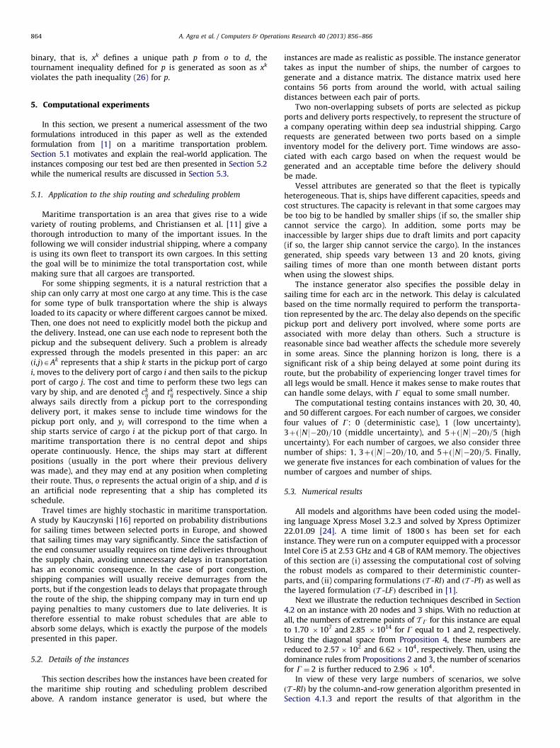
Next we illustrate the reduction techniques described in Section4.2 on an instance with 20 nodes and 3 ships. With no reduction atall, the numbers of extreme points of T G for this instance are equalto 1.70 �107 and 2.85 �1014 for G equal to 1 and 2, respectively.Using the diagonal space from Proposition 4, these numbers arereduced to 2:57� 102 and 6:62� 104, respectively. Then, using thedominance rules from Propositions 2 and 3, the number of scenariosfor G¼ 2 is further reduced to 2.96 �104.

In view of these very large numbers of scenarios, we solveðT -RIÞ by the column-and-row generation algorithm presented inSection 4.1.3 and report the results of that algorithm in the

A. Agra et al. / Computers & Operations Research 40 (2013) 856–866 865

following. In Table 1, we present the average number of extremepoints generated to solve ðT -RIÞ for each number of cargoes anduncertainty level. We see that these numbers are very smallcompared to the total number of reduced extreme points.

Table 2 reports the average numbers of cuts generated byðT -PIÞ for each number of cargoes and uncertainty level. We see thatðT -PIÞ generates significantly more cuts than ðT -RIÞ generatesextreme points. This can be explained by the fact that the cutsgenerated by ðT -PIÞ are tournament inequalities, which, as well asensure that the time windows are respected, also increases the linearprogramming relaxation. Hence, their violation is checked in everynode in the branch-and-cut tree solving ðT -PIÞ. In opposition to this,

Table 2Average numbers of cuts generated by ðT -PIÞ.

9N9 Uncertainty level (G)

Det Low Mid High

20 120 251 346 762

30 1210 313 867 795

40 25 097 9501 17 997 17 870

50 17 919 10 364 24 547 25 072

Table 3Average solution times in seconds for the three formulations for instances with

20 nodes.

G 9K9 ðT -LFÞ ðT -RIÞ ðT -PIÞ

Det Low Mid High Det Low Mid High Det Low Mid High

1 21 244 255 162 0.1 0.1 0.1 0.1 0.1 0.1 0.1 0.1

3 39.9 289 330 242 0.1 2.5 15.2 15.5 1.2 1.7 2.2 3.8

5 13.6 53 406 177 0.1 0.2 1.6 1.3 0.8 0.4 0.5 0.6

av 24.8 195 330 194 0.1 0.9 5.6 5.6 0.7 0.7 0.9 1.4

Table 1Average numbers of extreme points generated by

ðT -RIÞ.

9N9 Uncertainty level (G)

Low Mid High

20 2.93 7.2 7.67

30 3.1 9.33 9.13

40 6.67 20.7 21.7

50 7.93 22.8 23.2

Table 4Average solution times in seconds for ðT -RIÞ and ðT -PIÞ for larger instances.

9N9 G 9K9 ðT -RIÞ

Det Low Mid H

30 1 0.1 0.1 0.1 0

4 0.6 1.1 5.3 4

7 3.3 8.2 58.1 6

av 1.6 3.3 21.2 2

40 1 0.1 0.1 0.3 1

5 11.3 160 640 (2) 6

9 364 (1) 368 (1) 477 (1) 4

av 125 176 372 3

50 1 0.1 0.3 1.2 2

6 13.8 31.1 537 (1) 4

11 109 748 (2) 1070 (3) 9

av 41 260 536 4

the extreme points generated by ðT -RIÞ only enforce the satisfactionof the time windows. In addition, their necessity is checked only afteran optimal integer solution has been found for the previous set ofextreme points.

Average solution times are presented in Tables 3 and 4 for eachgroup of 5 instances. Rows entitled ‘‘av’’ compute the average of thethree rows above them. Table 3 provides average solution times forinstances with 20 nodes for the three formulations. Notice thatsolutions times for ðT -LFÞ assume that the instances have alreadybeen pre-processed by computing longest paths [1]. We see thatðT -RIÞ and ðT -PIÞ are about two orders of magnitude faster thanðT -LFÞ. Then, while ðT -RIÞ is faster than ðT -PIÞ for the deterministicinstances (G¼ 0), it is slower than ðT -PIÞ for the instances whereG40. Table 4 presents average solution times for the larger instancesfor formulations ðT -RIÞ and ðT -PIÞ. The numbers of unsolvedinstances within the 1800 s are given in parentheses and their valueshave been set to 1800 s when computing the averages. We see fromTable 4 that the performance of ðT -RIÞ and ðT -PIÞ are comparable,although ðT -RIÞ seems to be more efficient for the larger instances.The results for both approaches present, however, important differ-ences. The solution times for ðT -RIÞ are highly impacted by the valueof G. Deterministic instances are always solved faster than robustinstances. Moreover, the number of extreme points of the uncertaintysets also influences the solution times since instances with uncer-tainty sets defined by few extreme points (low) are solved faster thaninstances with uncertainty sets defined by larger number of extremepoints (mid and high). In opposition to this, the presence ofuncertainty does not seem to influence the solution times of ðT -PIÞ.

ðT -PIÞ

igh Det Low Mid High

.1 1 1.2 4.8 2.9

.1 2.9 1.6 1.7 2.1

6.1 27.3 7.6 16.6 17

3.4 10.4 3.5 7.7 7.3

.4 1.5 2.2 5.1 24

17 (2) 391 (1) 30 249 227

44 (1) 452 (1) 391 (1) 429 (1) 427 (1)

54 281 141 228 226

.8 6.7 7.3 28.2 55.3

85 (1) 534 (1) 216 805 (2) 779 (2)

62 (3) 1020 (3) 773 (2) 1160 (3) 1150 (3)

83 520 332 664 661

Table 5Cost of protecting the solution expressed as a percentage of the deterministic

solution cost.

9N9 G 9K9 Low Mid High Box

1 0.11 1.65 1.65 1.65

30 4 2.77 3.33 3.33 3.33

7 1.71 2.38 2.41 2.41

av 0.80 2.36 2.37 2.37

1 0.17 2.07 3.27 3.27

40 5 3.15 3.87 3.87 3.87

9 1.62 2.11 2.11 2.11

av 0.94 2.57 2.99 2.99

1 0.09 1.83 2.55 2.77

50 6 2.04 2.44 2.44 2.44

11 1.64 2.28 2.28 2.28

av 0.68 2.17 2.42 2.49

A. Agra et al. / Computers & Operations Research 40 (2013) 856–866866

Finally, Table 5 assesses the cost of protecting a solution againstdelays and compare these costs to the cost of protecting the solutionin the model where all travel times can take simultaneously theirmaximal values. The later model can be represented by thebox uncertainty set T box :¼ �kAK ,ði,jÞAAk ½t

kij,t

kijþ t

k

ij�. Let optmodel bethe optimal solution cost for modelAflow,mid,high,boxg. For eachgroup of 5 instances, we present the geometric mean increase ofsolution cost for model, computed as ðoptmodel�optdetÞ=optdet . We onlyconsider the instances for which we know the optimal solution costfor all models.

Notice that by using the dominance from Proposition 2, thebox uncertainty set can be replaced by the singleton ftþ tg,yielding a model that can be solved by ðT -RIÞ essentially as fastas the deterministic model. We can see in Table 5 that theprotection costs related to high and box are almost the same, sothat it seems more interesting to solve the model with a boxuncertainty set when a high protection is required.

6. Conclusion

This research addressed the vehicle routing problem with timewindows and travel times that belong to an uncertainty polytopeT . We presented two new formulations for the problem that arebased on resource inequalities ðT -RIÞ and path inequalities ðT -PIÞ,respectively, and extended well-known formulations for thedeterministic version of the problem.

Each formulation used different robust optimization tools tohandle the uncertainty. We proposed for ðT -PIÞ a new method tohandle the uncertainty implicitly with the help of canonical cuts,which did not increase the complexity of the formulation itself.Instead, this approach sent the additional complexity to theseparation routine. Then, formulation ðT -RIÞ relied on adjustablerobust optimization and we presented dominance rules thatsignificantly reduced the number of extreme points needed todefine the uncertainty polytope. We proposed efficient solutionalgorithms for both formulations: ðT -PIÞ was solved by a branch-and-cut algorithm while ðT -RIÞ was solved by a column-and-rowgeneration algorithm. We presented computational results per-formed on a set of instances that model a maritime transportationproblem using the budget uncertainty polytope studied in [7]. Theperformances of ðT -PIÞ and ðT -RIÞ were comparable for ourinstances and both formulations could handle problems withthe dimensions that arise in maritime transportation. In addition,the results showed that ðT -PIÞ is almost as easy to solve as itsdeterministic counterpart. This is a very interesting result since itcan be generalized to other robust combinatorial optimizationproblems. Hence, a side contribution of this work is the introduc-tion of an alternative approach to the dualization techniquehabitually used for static robust programming.

Ben-Tal et al. [4] proved that adjustable robust optimization iscomputationally intractable so that they introduced an approx-imation scheme that relied on affine decision rules. Despite itscomputational intractability, we have seen in this paper how wecould solve ðT -RIÞ efficiently by generating dynamically theextreme points of the polytope (or an equivalent set of scenarios).In view of the little number of scenarios generated by ouralgorithm, it is not necessary to approximate ðT -RIÞ with affinedecision rules. In fact, restricting y : T �R9A99K9-R9N9 to an affinefunction and dualizing the resulting models would yield mixed-integer programs much larger than the restricted versions ofðT -RIÞ we solved in this paper.

Acknowledgements

This research was carried out with financial support from theDOMinant II project, partly funded by the Research Council ofNorway. Agostinho Agra, Rosa Figueiredo, and Cristina Requejoare supported by FEDER founds through COMPETE-OperationalProgramme Factors of Competitiveness and by Portuguese foundsthrough the CIDMA (University of Aveiro) and FCT, within projectPEst-C/MAT/UI4106/2011 with COMPETE number FCOMP-01-0124-FEDER-022690. Michael Poss was supported by FCT underthe postdoctoral scholarship SFRH/BPD/76331/2011 and the grantPEst-C/MAT/UI0324/2011. The authors are grateful to the refereesfor their careful readings of the work.

References

[1] Agra A, Christiansen M, Figueiredo R, Magnus Hvattum L, Poss M, Requejo C.Layered formulation for the robust vehicle routing problem with timewindows. In: Lecture Notes in Computer Science, vol. 7422/2012; 2012, p.249–60.

[2] Ascheuer N, Fischetti M, Grotschel M. A polyhedral study of the asymmetrictraveling salesman problem with time windows. Networks 2000;36:69–79.

[3] Balas E, Jeroslow R. Canonical cuts on the unit hypercube. SIAM Journal onApplied Mathematics 1972;23:61–79.

[4] Ben-Tal A, Goryashko A, Guslitzer E, Nemirovski A. Adjustable robustsolutions of uncertain linear programs. Mathematical Programming2004;99:351–76.

[5] Ben-Tal A, Nemirovski A. Robust solutions of uncertain linear programs.Operations Research Letters 1999;25:1–13.

[6] Bertsimas D, Brown DB, Caramanis C. Theory and applications of robustoptimization. SIAM Review 2011;53:464–501.

[7] Bertsimas D, Sim M. The price of robustness. Operations Research2004;52:35–53.

[8] Bienstock D, Ozbay N. Computing robust basestock levels. Discrete Optimiza-tion 2008;5:389–414.

[9] Chardy M, Klopfenstein O. Handling uncertainties in vehicle routing pro-blems through data preprocessing. Transportation Research Part ELogisticsand Transportation Review. 2012;48:667–83.

[10] Christiansen CH, Lysgaard J. A branch-and-price algorithm for the capacitatedvehicle routing problem with stochastic demands. Operations ResearchLetters 2007;35:773–81.

[11] Christiansen M, Fagerholt K, Nygreen B, Ronen D. Maritime transportation.Handbooks in operations research and management science. vol. 14; 2007. p.189–284 [chapter].

[12] Codato G, Fischetti M. Combinatorial Benders’ cuts for mixed-integer linearprogramming. Operations Research 2006;54:756–66.

[13] Desaulniers G, Villeneuve D. The shortest path problem with time windowsand linear waiting costs. Transportation Science 2000;34:312–9.

[14] Golden B, Raghavan S, Wasil EA. The vehicle routing problem: latest advancesand new challenges. In: Operations Research/Computer Science InterfacesSeries, vol. 43. Boston: Springer; 2008.

[15] Kallehauge B, Boland N, Madsen OBG. Path inequalities for the vehiclerouting problem with time windows. Networks 2007;49:273–93.

[16] Kauczynski W. Study of the reliability of the ship transportation. In:Proceeding of the international conference on ship and marine research;1994.

[17] Miller CE, Tucker AW, Zemlin RA. Integer programming formulation oftraveling salesman problems. Journal of the ACM 1960;7:326–9.

[18] Ordonez F. Robust vehicle routing. TutORials in Operations Research2010:153–78.

[19] Oriolo G. Domination between traffic matrices. Mathematics of OperationsResearch 2008;33:91–6.

[20] Poss M, Raack C. Affine recourse for the robust network design problem:between static and dynamic routing. Networks, http://dx.doi.org/10.1002/net.21482 in press.

[21] Righini G, Salani M. New dynamic programming algorithms for the resourceconstrained elementary shortest path problem. Networks 2008;51:155–70.

[22] Soyster AL. Convex programming with set-inclusive constraints and applica-tions to inexact linear programming. Operations Research 1973;21:1154–7.

[23] Subramanian A, Uchoa E, Pessoa AA, Satoru Ochi L. Branch-and-cut with lazyseparation for the vehicle routing problem with simultaneous pickup anddelivery. Operations Research Letters 2011;39:338–41.

[24] FICO Xpress Optimization Suite, Xpress-Optimizer reference manual. Tech-nical Report Release 22.01, 2011.

[25] Sungur I, Ordonez F, Dessouky M. A robust optimization approach for thecapacitated vehicle routing. IIE Transactions 2008;40:509–23.