Discrete Latent Markov Models for Normally Distributed Response Data

Discrete Latent Markov Modelsfor Normally Distributed Response Data

Verena D. Schmittmann, Conor V. Dolan,and Han L. J. van der Maas

Department of PsychologyUniversity of Amsterdam

Michael C. NealeDepartments of Psychiatry & Human Genetics

Virginia Commonwealth University

Van de Pol and Langeheine (1990) presented a general framework for Markov mod-eling of repeatedly measured discrete data. We discuss analogical single indicatormodels for normally distributed responses. In contrast to discrete models, which havebeen studied extensively, analogical continuous response models have hardly beenconsidered. These models are formulated as highly constrained multinormal finitemixture models (McLachlan & Peel, 2000). The assumption of conditional inde-pendence, which is often postulated in the discrete models, may be relaxed in the nor-mal-based models. In these models, the observed correlation between two variablesmay thus be due to the presence of two or more latent classes and the presence ofwithin-class dependence. The latter may be subjected to structural equation model-ing. In addition to presenting various normal-based Markov models, we demonstratehow these models, formulated as multinormal finite mixtures, may be fitted using thefreely available program Mx (Neale, Boker, Xie, & Maes, 2002). To illustrate the ap-plication of some of the models, we report the analysis of data relating to the under-standing of the conservation of continuous quantity (i.e., a Piagetian construct).

The aim of this article is to present and apply a general model for change and sta-bility in latent class membership, where this membership at each occasion is in-ferred from an observed continuous indicator variable. The vector of the repeat-edly measured indicator variable is assumed to be multinormally distributed, when

MULTIVARIATE BEHAVIORAL RESEARCH, 40(4), 461–488Copyright © 2005, Lawrence Erlbaum Associates, Inc.

The authors thank the reviewers for many useful comments. The research of Conor V. Dolan hasbeen made possible by a fellowship of the Royal Netherlands Academy of Arts and Sciences. The re-search of Michael C. Neale and the development of Mx were supported by NIH grants MH-65322 andRR-08123.

Correspondence concerning this article should be addressed to Verena Schmittmann, Departmentof Psychology, University of Amsterdam, Roetersstraat 15, 1018 WB Amsterdam, The Netherlands.E-mail: [email protected]

conditioned on sequences of latent classes. The latent class variable comprisesqualitatively different categories, for example, cognitive stages or strategies, orpresence and absence of psychological illness. Change over time is accounted forby transitions between the classes. Thus the kind of change we aim to model isqualitative, as opposed to smooth quantitative change, which is assumed in, for in-stance, latent growth curve models (e.g., Reise & Duan, 2003).

The general model may be viewed as analogous to van de Pol and Langeheine’s(1990) mixedMarkov latent class (MMLC)model fordiscrete (categorical) longitu-dinal data. The two building blocks of their framework are latent class models(LCM; Lazarsfeld & Henry, 1968), and Markovian transition models (Kemeny &Snell, 1976). In the LCM, the categorical variable observed at each occasion istreated as a possibly fallible indicator of latent classes. The Markov model is positedto accommodate switching over time in class membership. For example, given classA and B, possible transitions are A-A, A-B, B-A, and B-B. In the simplest case, theprobability of each sequence over time of latent classes (e.g., over two time pointsAA, AB, BA, BB) is given by the product of the probability of being in the specificclassat the first occasion, and theconditionalprobabilityof remaining in this classorswitching. The MMLC framework includes a large number of special cases.

In the general model considered here, the Markov model is retained, but the dis-crete distributions of the data are replaced by conditional multinormal distribu-tions. The present model is an analogue of the MMLC framework in the followingsense. Consider, for instance, the following two static models with multiple indica-tors: the latent class model (LCM) and the latent profile model (LPM;Bartholomew & Knott, 1999; Lazarsfeld & Henry, 1968). In both models, a finitenumber of latent classes are posited. Both models may be viewed as a finite mix-ture model, where the latent classes represent distinct mixture components (seeMcLachlan & Peel, 2000; Wolfe, 1970). The only difference lies in the distributionof the observed variables, conditioned on (i.e., within) the latent classes. In theLCM, it is discrete, for example, multinomial; in the LPM, it is multinormal. Simi-larly, the more general MMLC models of van de Pol and Langeheine (1990) andthe normal analogue considered here can be viewed as finite mixture models,where each unique sequence of latent classes (e.g., AAAB) represents a distinctmixture component. In fitting the normal analogue models, we treat them explic-itly as multinormal finite mixture models (McLachlan & Peel, 2000). Given thistreatment, we may relax the independence assumption, which is posited in theMMLC models (but see Hagenaars, 1988; Uebersax, 1999).

The class of models discussed by van de Pol and Langeheine (1990) hasreceived considerable attention (e.g., Collins & Wugalter, 1992; Thomas & Hett-mansperger, 2001), whereas the present class of models has received much less at-tention in the social sciences (but see Hamilton, 1994; Kim & Nelson, 1999;McLachlan & Peel, 2000, for applications in other areas). The only application, ofwhich we are aware, is by Dolan, Jansen, and van der Maas (2004). They fitted spe-cial cases of the present general model to a cognitive development data set. They

462 SCHMITTMANN, DOLAN, VAN DER MAAS, NEALE

did not relate their models to the discrete analogues, as described in van de Pol andLangeheine, nor did they discuss the relation of their model with the generalmodel. The general model presented here comprises the models that are inheritedfrom the analogous discrete framework, for example, the models that Dolan et al.fitted, and many other models, such as multiple chain, and multi-group models, ormodels with a more complex within-component covariance structure. Further-more, rather than using the same indicator variable at each occasion, the presentmodel allows for the use of different indicator variables at each occasion. Becauseof this flexibility, the present model can be used in novel contexts, such as experi-mental studies, in which item characteristics are manipulated experimentally, andswitching between classes is seen as an effect of the manipulation.

Examples for Markov models with discrete or discretized indicators can befound in studies on the course of clinical depression (e.g., Wolfe, Carlin, & Patton,2003), or Alzheimer’s Disease (Stewart, Phillips, & Dempsey, 1998). The presentmodel may be useful in similar contexts. One example is the study of body mass in-dex (BMI) and self-esteem in a sample of nonpurging type bulimia patients, whoalternate between binging and fasting or exercising, and in the analysis ofpsychometric mood scores in a sample of bipolar patients, who alternate betweenan asymptomatic, a manic, and a depressed state. The illustrations presented belowstem from the area of cognitive development, where the Piagetian theory (Piaget &Inhelder, 1969) predicts progression via a small number of hierarchically orderedlatent classes.

The discrete models can be fitted with various programs, for example,PANMARK (van de Pol, Langeheine, & de Jong, 1989), WinLTA (Collins,Lanza, Schafer, & Flaherty, 2002), or LEM (Vermunt, 1997). Dolan et al. (2004)used their own FORTRAN programs to fit their models using maximum likeli-hood (ML) estimation. We use the program Mx (Neale et al., 2002) to fit thepresent models by ML estimation.1 Example Mx input files and analyzed datasets may be downloaded at the Mx script library.2

The outline of this article is as follows. First, we briefly introduce cognitive de-velopment as a field of application. This provides various concrete examples, towhich we return in presenting the model. After describing the model, we discussthe estimation procedure and the assessment of goodness of fit. Then, we presentillustrative analyses of two different data sets, both relating to the Piagetian con-cept of the conservation of continuous quantity (Piaget & Inhelder, 1969). In thefirst illustration, we apply seven submodels of the general model to data from alongitudinal study, in which the concept of the conservation of a continuous quan-tity is measured repeatedly with the same indicator variable. In the second illustra-tion, we fit other submodels to data from an experimental study, in which the sameconcept is measured repeatedly with an experimentally manipulated indicator.

MARKOV MODELS FOR NORMAL DATA 463

1Mx can be downloaded at http://www.vcu.edu/mx/2The URL of the Mx script library is http://www.psy.vu.nl/mxbib/

AREA OF APPLICATION

The Piagetian theory of cognitive development predicts that children in a certain agerange belong to one of a small number of latent classes, or stages (Piaget & Inhelder,1969). For instance, children between the ages 4 and 12 are in the pre-operational orconcrete operational stage. Although the generality of the stage theory of Piaget hasbeen criticized (Flavell, 1971), this theory has proved useful in studies of domainspecificdevelopment. Illustrativedomainsareproportional reasoning,horizontalityof liquid surfaces, and conservation (Boom, Hoijtinck, & Kunnen, 2001; Jansen &van der Maas, 2001; Thomas & Hettmansperger, 2001). Within these domains, welldefined tasks, such as the balance scale task, the water level task, and the conserva-tion anticipation task discriminate well between children in different stages.

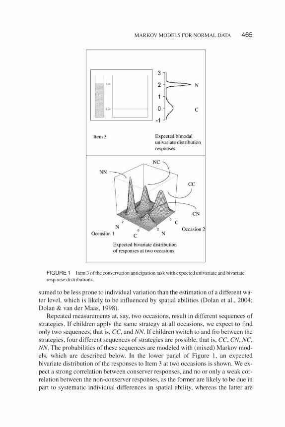
The conservation anticipation task is used to assess the ability to conserve con-tinuous quantity. In the upper panel of Figure 1, a typical item is shown, as used inIllustration 1 below.3 On each item, children are required to predict and indicatethe water level in the event that the water in the left glass is poured into the glass onthe right side. Children in the appropriate age range are expected to respond ac-cording to one of two distinct strategies, which characterize their cognitive stage.Simply aligning the water level at the same height is typical of the pre-operationalstage. We refer to this strategy as non-conserver strategy (N). Adjusting the waterlevel to compensate for the different shapes of the vessels is typical of the concreteoperational stage. We refer to this strategy as conserver strategy (C). The transitionfrom the pre-operational stage to the concrete operational stage is expected toprogress via an unstable transition phase, in which children may switch betweenboth strategies (e.g., van der Maas & Molenaar, 1992).

Although children are expected to respond according to one of two distinctstrategies, their responses are measured on a continuous scale. In Figure 1, next toItem 3, the expected two-component normal mixture distribution of the observedvariable height of the predicted water level, is shown. One component representsthe responses of the non-conservers with an expected mean equal to the water levelin the left glass. The second component represents the responses of the conservers,with an expected mean equal to the correctly adjusted water level. The variance ofthe conserver strategy responses is expected to be larger than the variance of thenon-conserver strategy responses, because merely carrying out an alignment is as-


3The vessels are depicted two-dimensionally in the computer-based and pen-and-paper versions ofthe task (example 1 and 2, respectively), whereas the original volume conservation task uses real glasses.Therefore, we cannot be completely sure if such a representation of the task measures the ability to con-servevolumeorsurface/area.This issuewasaddressed inanadditional small studywith two-dimensionalrepresentations. The results indicated that responses on a surface-rule based conservation task correlatedhighly (about .79) with responses to a volume-rule based conservation task. However, as the volume-rulebased taskappeared tobemoredifficult,werefer to the taskasaconservation task forcontinuousquantity.We employ expected values that are based on the surface rule. The expected values based on the area rulediffer, but the transitive relation between the water levels of different items stays the same.

sumed to be less prone to individual variation than the estimation of a different wa-ter level, which is likely to be influenced by spatial abilities (Dolan et al., 2004;Dolan & van der Maas, 1998).

Repeated measurements at, say, two occasions, result in different sequences ofstrategies. If children apply the same strategy at all occasions, we expect to findonly two sequences, that is, CC, and NN. If children switch to and fro between thestrategies, four different sequences of strategies are possible, that is, CC, CN, NC,NN. The probabilities of these sequences are modeled with (mixed) Markov mod-els, which are described below. In the lower panel of Figure 1, an expectedbivariate distribution of the responses to Item 3 at two occasions is shown. We ex-pect a strong correlation between conserver responses, and no or only a weak cor-relation between the non-conserver responses, as the former are likely to be due inpart to systematic individual differences in spatial ability, whereas the latter are


FIGURE 1 Item 3 of the conservation anticipation task with expected univariate and bivariateresponse distributions.

likely to reflect only unsystematic errors. In other words, we expect variable andcorrelated responses in the conservers and uncorrelated and much less variable re-sponses in the non-conservers. Responses originating from different strategies areexpected to be uncorrelated. We return to this example in the presentation of themodel and in the illustrations.

MIXED MARKOV LATENT STATE MODELSFOR MULTINORMAL DATA

The model description begins with the Markov models (van de Pol & Langeheine,1990). These accommodate switching between latent classes over time, andthereby constrain the probabilities of all sequences of classes. Then, we discusshow the sequences of latent classes are linked to the observed responses: First, weformulate the probability distribution of the indicator variables as a multinormal fi-nite mixture distribution. Second, we describe the within-component model andthe constraints on the parameters of the multinormal finite mixture distribution,and show how the independence assumption may be relaxed.

Markov Models

Markov models have been used widely in psychological research (see Wickens,1982, for an overview). Here, we consider discrete-time first-order Markov mod-els. Finite-state Markov processes are characterized by the following properties.

1. Finite set of states. The state of the process at any time is one of a finite set ofstates sk, k = 1, …, S. In the example of the previous section, we have two states.Subjects applying the conserver (non-conserver) strategy are in the conserver stateC, and subjects who apply the non-conserver strategy are in the non-conserverstate N.

2. Transition probabilities of moving from state sk to state sl at time i. Ifthe transition probabilities do not change with time, the process is called station-ary, and the probabilities can be collected in a single transition matrix � with

(Kemeny & Snell, 1976). To ease presentation, we focus on stationarymodels. These can easily be extended to accommodate nonstationarity (see Illus-trations that follow). Each column of the transition matrix sums to 1. In the exam-ple, the 2 × 2 transition matrix � contains the probabilities of remaining in state Cand N (�C|C, and �N|N), and the probabilities of switching from state C to N (�N|C), orvice versa (�C|N):


l kis s

�

l klk s s� ��

.C C C N

N C N N

� �

� �

� ��

� �

�

3. A vector � with initial probabilities �k. The process starts in state sk with prob-ability �k.4 In the example, the initial probability vector � = (�C, �N)t contains theprobabilities to start in the conserver (�C) and non-conserver state (�N).5 The sumof the initial probabilities equals one.

4. The Markov property. This property states that knowledge of the history ofthe process prior to the present state does not add any information in a first ordermodel (see Kemeny & Snell, 1976, p. 24 for a formal definition).

These four properties define a Markov model, or Markov chain. To ease presen-tation, but without loss of generality, we formulate models for two states, namely Nand C. Consider first a homogeneous population, in which the same initial andtransition probabilities apply to all subjects. The probability PNNC of sequenceNNC equals the product of the initial probability of state N, the probability of re-maining in state N, and the probability of switching from state N to state C, PNNC =�N · �N|N · �C|N. In general, let s(i), i = 1, …, T denote the state of a subject at time i.In the single Markov chain model, the unconditional probability, Ps, that a givenmember of the population follows a certain sequence s of states s(1), s(2), ..., s(T)equals the product of the initial probability of the first state �s(1), and of the respec-tive transition probabilities �s(i+1)|s(i):

Ps = �s(1) · �s(2)|s(1) · … · �s(T)|s(T–1). (1)

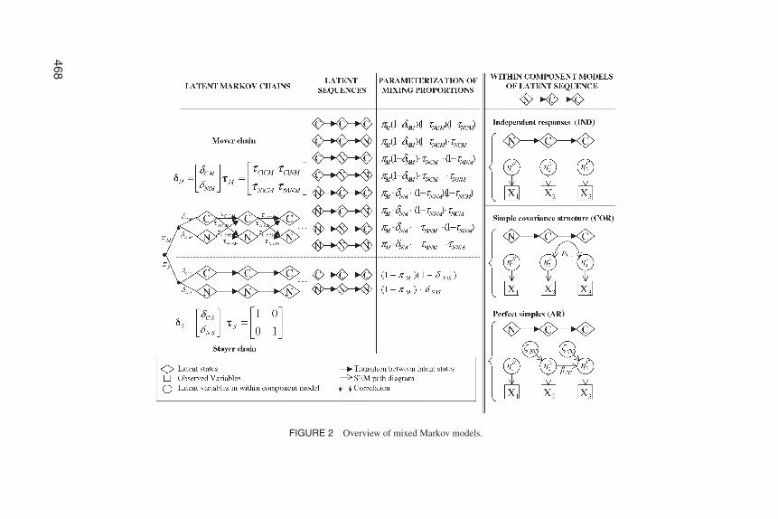
The assumption of homogeneity of the sample may be relaxed in two ways.First, we may have two or more samples, which are drawn from observable popu-lations, such as males and females, or experimental and control group. In this case,we may introduce a Markov chain in each sample, that is, we carry out amulti-group analysis, and we may test for equalities of the parameters (e.g., initialprobabilities, transition probabilities) over the groups. Second, we may suspectthat our sample is representative of two or more populations, which are not directlyobserved. We call these latent populations to distinguish them from observed pop-ulations. For example, a sample of children in a broad age range (e.g., 5 to 12years) may consist of children in the transition phase, who may switch between theC and N strategy (henceforth: movers), and of children in the pre-operational orconcrete operational stage, who respond consistently (henceforth: stayers). Herewe model the heterogeneity by specifying a mixture of latent Markov chains, asshown on the left part of Figure 2. The latent chains have distinct initial and transi-tion probabilities. The additional parameters �M and �S denote the probability ofbelonging to the mover chain (M) and the stayer chain (S), respectively. In the mid-dle part of Figure 2, all resulting latent sequences are shown. Note, that the two la-


4Note that in stationary, ergodic Markov chains the initial probability vector �may be constrained toequal the stationary distribution of the transition matrix �, such that � = � · � (Kemeny & Snell, 1976).

5Superscripted t denotes transposition.

468

FIGURE 2 Overview of mixed Markov models.

tent sequences of the stayer chain also occur in the mover chain, as some subjectsin the transition phase could also respond according to one strategy at all occa-sions. Adding the stayer chain can accommodate an excess number of stayers. Inaddition, we can have the nested case of two or more latent populations withinmultiple samples. Consider for example the situation in which boys and girls in abroad age range have been assessed repeatedly on a conservation task. Assumingwe have recorded gender, we may specify a multi-group model. Within the sampleof boys (same applies to the girls), heterogeneity may be present due to the fact thatthe boys are drawn from different latent populations. The sample of boys may in-clude movers and stayers. Such heterogeneity is accommodated by specifying amixture of latent Markov chains. Thus the presence of boys and girls is accommo-dated by specifying a multi-group model, while possible heterogeneity within thesample of boys and girls is accommodated by specifying a mixture of latentMarkov chains. Again we may investigate whether the parameters of the latentMarkov chains are equal over the groups.

In general, if a sample is drawn from L latent populations, van de Pol andLangeheine (1990) specify a mixture of L latent Markov chains. In the mixedMarkov model for L latent chains in G observed groups or samples, the uncondi-tional probability of belonging to group g, with observed proportion �g, and of fol-lowing a certain sequence s is given by

where �l|g denotes the probability of being in chain l, conditioned on group g. Thisis the most general model, as it includes all the other models as special cases.6 It re-duces to a mixed Markov model for L latent chains in one sample, if G = 1 (�g = 1).


6As van de Pol and Langeheine (1990) remark, a mixed Markov model with L chains, in which eachchain (with associated chain probability �l) consists of a finite set of states Sl, a transition matrix �l, andan initial probability vector �l, can be rewritten as a single Markov model with transition matrix � andwith initial probability vector �:

For the same reason, it is possible to conceive of the mover-stayer model as well as a two-chain modelwith identity transition matrix in the stayer chain, and as a three-chain model with only one state in eachof the two stayer chains.

11

1

222

1

0 0 01

0 0 0, .

0 0 0

0 0 01L

LL

�

�

�

�

�

��

�

�

��

= =

Ł ł

Ł ł

� � � � � , 1 2 1 11

... , (2)L

g g l g s lg s s lg s T s T lgl

P � � � � �

�

� �s

Conversely, when L = 1 (�l|g = 1), we have a multi-group model for G groups with asingle latent Markov chain in each group.

A variety of hypotheses may be tested by imposing different constraints on thetransition probabilities (see the Illustrations for some examples, and Wickens,1982, for an overview). The Markov models given in Equations 1 and 2 apply tothe sequences of latent states. They do not include a model that links the manifestindicator variables to the latent states. This is discussed in the next sections.

Multinormal Mixture Models

We specify a multinormal mixture distribution, with a distinct component for eachsequence of latent states, given chain and group. First, we present the standard no-tation of the finite multinormal mixture density (McLachlan & Peel, 2000). Then,we show how this density reduces to the highly constrained normal analogues ofthe discrete mixed Markov models of van de Pol and Langeheine (1990). TheM-component multinormal mixture density is defined as follows:

The T-dimensional vector xj contains the repeated measures of subject j (j = 1, 2,…, N). All vectors are column vectors. The [T × (T · M)] matrix � contains M (T ×T)-dimensional positive definite, but otherwise unconstrained covariance matri-ces, � = [�1, �2, …, �M]. The (T · M)-dimensional vector � contains M T-dimen-sional mean vectors The M-dimensional vector p containsthe mixing proportions, p = [p1, p2, …, pM]t, which may be viewed as probabilities:

and 0 ≤ pi ≤ 1. The ith component distribution equals:

that is, the T-variate normal density with (T × T) covariance matrix �i and T-di-mensional mean vector �i (McLachlan & Peel, 2000). denotes the determi-nant of �i.

In the mixed Markov latent state models for multinormally distributed data, a dis-tinct component is specified for each latent sequence, given chain and group. There-fore, the total number of components in an otherwise unconstrained model equalsthe sum of the number of all possible sequences in all chains in all groups. Consider


� �

� � �

1/ 2 1/ 2 1/ 2; , 2 , (4)t

j j iiT ii j i i if e�

�

x xx � � ��

1 2, , .tt t t

M�

��

� � � ��

� 1

1M

iip

�

��

� �

1

; , , ; , . (3)M

j i i j i ii

f p f�

� �x p x� � � �

i�

for instance, the model shown in Figure 2, which contains 10 sequences at three oc-casions (8 from the mover chain, and 2 from the stayer chain). In an unconstrainedmixture model as in Equation 3 with 10 components, we would estimate 9 mixingproportions. But in the mixed Markov latent state models, the mixing proportions ofthe components equal the probabilities of the sequences. These are constrained bythe mixed Markov model. Let the vector � contain the free parameters of the mixedMarkov model. For instance, Figure 2 shows the parameterization of the mixing pro-portions of a mover-stayer model at 3 occasions with two latent states in one group interms of � = (�M, �N|M, �N|NM, �N|CM, �N|S). In general, the number of free parameters,used to model the mixing proportions, is reduced from (M -1) in the unconstrainedmodel in Equation 3 to the number of free initial, chain, and transition probabilities.Consider first the mixed Markov model in one sample, as given in Equation 2, withG = 1 and �g = 1, where each sequence in each chain corresponds to a component.Equation3cannowberewritten to include theconstraintson themixingproportions.The density f[xj; �(�), �(�), p(�)] of the responses is given by:

where represents the mixing proportion of se-quence s of chain l. The vector � contains the parameters that are used to modelthe covariance matrix and the mean vector, and the vectors �sl (subset of �) con-tain the parameters that are used to model the covariance matrix and the mean vec-tor within the component of chain l and sequence s. In Equation 5, we write �, �,and p as a function of the parameter vectors � and � to indicate the constraints, asopposed to the unconstrained model in Equation 3. The multinormal density fsl[xj;�(�sl), �(�sl)] of the responses within a component, that is, given latent chain l,and sequence s of latent states s = s(1), s(2), …, s(T) is specified as:

that is, the T-variate normal density with (T × T) covariance matrix �(�sl) and T-di-mensional mean vector �(�sl). In the case of G groups the unconditional distribu-tion of the responses is given by:


� �

� � � �

11/ 2/ 2 1/ 2

; ( ), ( )

2 , (6)t

j l l j l

l j l l

Tl

f

e � � � � � �

� � � �

� � �

� � � � � ��

� ��

x x

x

s s s

s s s

s

� � �

� � � � �

�

� �

�

� �

2 2

1 2 1 11 1 1 1

; , ,

; , , (5)

j

L

l l j l ls l s s l s T s T ll s s T

f

f� � � �

� � �

� �

� �

� �

� ��

x p

xs s s

� � � � �

� � � �

� � � � � 1 2 1 1l s l s s l s T s T l� � � �

�

� �

�

� � � � � �

1

; , , ; , , , (7)G

j g g jg g g gg

f f��

� � � �

� �� x p x p� � � � � � � � � �

where is the distribution of the responses, as ex-pressed in Equation 5, of group g. In the next section the general model for thecovariance matrix and the mean vector in each component is presented.

Within-Component Models

Within each component s, that is, for each distinct sequence s of latent states, in eachchain c and each group g, we specify the following manifest LISREL submodel(Jöreskog & Sörbom, 2002). The general measurement equation of subject j is:

xj = �slg + �slgslg j + scg j, (8)

where �slg is a T-dimensional vector of the means, �slg is a (T × T) matrix of factorloadings, slg j a T-dimensional random vector of zero mean latent variables, andscg j is a T-dimensional random vector of residual terms that are distributed aszero-mean normals. The structural equation is

slg j = Bslgslg j + �slg j, (9)

where Bslg is a (T × T) matrix of regression coefficients, and �slg j is a T-dimensionalrandom vector of zero mean residuals, which is uncorrelated with slg j. Below, wedo not require the residuals scg j, because the applications involve single indicatormodels. In the case of multiple indicator models the scg j term may be useful.Equations 8, discarding the residual terms scg j, and 9 imply the followingcovariance matrix and mean vector within the components:

where �slg is the (T × T) covariance matrix of the residuals �slg j, and I is the (T × T)identity matrix.

Several substantively motivated and identifying constraints are placed on the pa-rameters. Within each latent chain and group, the means of a specific indicator vari-able (i.e., height of the predicted water level on Item 3), given a latent state and occa-sion, areconstrained tobeequaloverall sequences.Likewise, theparametersused tomodel the covariance matrices of the different sequences are constrained to be equalwithin a latent chain and group. In both illustrations below, we impose the followingsubstantively motivated constraints. We assume that the response strategy given asequence of conserver and non-conserver states does not differ between differentgroups, or different chains. Therefore, the component distributions of a specific se-quence of latent states are constrained to be identical, for example, the componentdistribution of sequence CCCCC in the mover chain equals the component distribu-tion of the same sequence CCCCC in the stayer chain. As mentioned above, we as-


� � �

�

1 1

and , (10)

t tlg lg lg lg lg lg

lg lg

� � � �

� �

�

�

I B I Bs s s s s s

s s

� � � ; , ,g jg g g gf �

� ��

x p� � � � �

sume that the response strategy, given a latent state, leads to the same mean responseto a given item at different occasions. So, we constrain the means of the response dis-tributions at different occasions, given a latent state, to be equal, whenever the sameindicator variable is used. For instance, in the first illustration, the mean vector of thecomponent of sequence s = CCNNC, equals �s = [�C, �C, �N, �N, �C]t, as the sameitem is used at all occasions. In the second illustration, Item 1 is used at the first andfifth occasion, Item 2 at the second and fourth, and Item 3 at the third occasion (seeFigure 3). The mean vector of, for example, sequence s = CCNNC equals �s = [�C1,�C2, �N3, �N2, �C1]t. The similar constraints on the covariance matrices are dis-cussed in the next paragraphs, where we consider three special cases of the LISRELmodel in Equation 10: A model with independent responses, a simple covariancestructuremodel, andaperfect simplexmodel.On the right-handsideofFigure2pathdiagrams of these three special cases in one exemplary component are shown. As theperfect simplex model is a time series model, it is suitable in Illustration I. All threemodels are illustrated below. As the LISREL model in Equation 10 is quite general,many other models may be considered.

Independent Response Model

This model is the most simple, as it assumes independent variables, that is, thecovariance matrices within the components are diagonal. In this case, themultinormal response density in Equation 6 equals the product of the univariatenormal densities. This model may be viewed as a constrained latent profilemodel. Within each component, we specify:

where the diagonal elements diag(�slg) = [�s(1)lg, �s(2)lg, …, �s(T)lg] of �slg are thestandard deviations within the component of sequence s in chain l, and group g. In Il-lustration I below, we impose the following equality constraints on the standard de-viations �s(i)lg. Given a latent state C and N, we specify a standard deviation �C and�N, independent of measurement occasion, chain, and group. The vector � containstwo means and two standard deviations. For instance, the diagonal elements of the


FIGURE 3 Analyzed items of the paper-and-pencil hysteresis conservation anticipation task.The original widths of the empty glass of Items 1 to 3 equal 4.2, 5.6 and 6.3 cm, respectively.Children were required to draw a line at the predicted water level of the amount of liquid in theleft glass when the water is poured into the right glass.

� , (11)tlg lg lg� Is s s� � � �

matrix �s of the component of sequence s = CCNNC, equal diag(�s) = [�C, �C, �N,�N, �C].

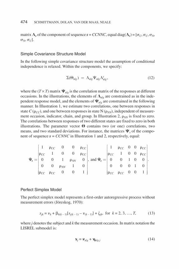
Simple Covariance Structure Model

In the following simple covariance structure model the assumption of conditionalindependence is relaxed. Within the components, we specify:

where the (T × T) matrix �slg is the correlation matrix of the responses at differentoccasions. In the illustrations, the elements of �slg are constrained as in the inde-pendent response model, and the elements of �slg are constrained in the followingmanner. In Illustration 1, we estimate two correlations, one between responses instate C (�CC), and one between responses in state N (�NN), independent of measure-ment occasion, indicator, chain, and group. In Illustration 2, �NN is fixed to zero.The correlations between responses of two different states are fixed to zero in bothillustrations. The parameter vector � contains two (or one) correlations, twomeans, and two standard deviations. For instance, the matrices �s of the compo-nent of sequence s = CCNNC in Illustration 1 and 2, respectively, equal:

Perfect Simplex Model

The perfect simplex model represents a first-order autoregressive process withoutmeasurement errors (Jöreskog, 1970):

xjk = k + k(k – 1)[xj(k – 1) – (k – 1)] + �jk, for k = 2, 3, …, T, (13)

where j denotes the subject and k the measurement occasion. In matrix notation theLISREL submodel is:

xj = slg + slg j (14)


1 0 0 1 0 0

1 0 0 1 0 0

, and .0 0 1 0 0 0 1 0 0

0 0 1 0 0 0 0 1 0

0 0 1 0 0 1

CC CC CC CC

CC CC CC CC

NN

NN

CC CC CC CC

� � � �

� � � �

�

�

� � � �

� �

� � � �

� � � �

� � � �

� � � ��

� � � �

� � � �

� � � �

� � � �

� � � ��

s s� �

( ) , (12)tlg lg lg lg� � � ��s s s s

slg j = Bslgslg j + �slg j. (15)

Within the components we specify:

�(�slg) = (I – Bslg)–1�slg(I – Bslg)–1t. (16)

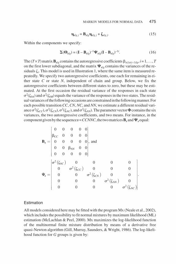
The (T × T) matrix Bslg contains the autoregressive coefficients s(i)s(i–1)lg, i = 1, …, Ton the first lower subdiagonal, and the matrix �slg contains the variances of the re-siduals �i. This model is used in Illustration 1, where the same item is measured re-peatedly. We specify two autoregressive coefficients, one each for remaining in ei-ther state C or state N, independent of chain and group. Below, we fix theautoregressive coefficients between different states to zero, but these may be esti-mated. At the first occasion the residual variance of the responses in each state�2(�0A) and �2(�0B) equals the variance of the responses in the two states. The resid-ualvariancesof thefollowingoccasionsareconstrained in thefollowingmanner.Foreach possible transition CC, CN, NC, and NN, we estimate a different residual vari-ance �2(�CC), �2(�CN), �2(�NC), and �2(�NN). The parameter vector � contains the sixvariances, the two autoregressive coefficients, and two means. For instance, in thecomponentgivenbythesequences=CCNNC, the twomatricesBs and�s equal:

Estimation

All models considered here may be fitted with the program Mx (Neale et al., 2002),which includes the possibility to fit normal mixtures by maximum likelihood (ML)estimation (McLachlan & Peel, 2000). Mx maximizes the log-likelihood functionof the multinormal finite mixture distribution by means of a derivative freequasi-Newton algorithm (Gill, Murray, Saunders, & Wright, 1986). The log-likeli-hood function for G groups is given by:


�

�

�

�

�

20

2

2

2

2

0 0 0 0 0

0 0 0 0

, and0 0 0 0 0

0 0 0 0

0 0 0 0 0

0 0 0 0

0 0 0 0

.0 0 0 0

0 0 0 0

0 0 0 0

CC

NN

C

CC

CN

NN

NC

� �

� �

� �

� �

� �

�

� �

� �

� �

� ��

� �

� �

� �

� �

� ��

�

� �

� �

� �

� ��

� �

� �

� �

� �

� ��

Bs

s�

where Ng denotes the number of subjects in group g,

denotes the

data matrix, and fg[xjg; �(�g), �(�g), p(�g)] denotes the multivariate mixturedensity of the responses in group g (see Equation 7). Mx can handle missing dataunder the assumption that the data are missing at random or missing completely atrandom (Little & Rubin, 1989; Muthén, Kaplan, & Hollis, 1987; Wothke, 2000).Mx does not calculate standard errors but does include the possibility to calculatelikelihood-based confidence intervals of the parameter estimates. We report 90%confidence intervals of parameters of particular interest.

MODEL COMPARISON

Hypotheses concerning the covariance matrices, mean vectors, and mixing propor-tions of the components can be tested by means of the likelihood ratio test if themodels are nested (e.g., Yung, 1997). In contrast, hypotheses relating to the num-ber of components cannot be tested in this manner (McLachlan & Peel, 2000). Werely on two commonly used information criteria for model comparison: theBayesian Information Criterion (BIC; Schwarz, 1978) and the Akaike InformationCriterion corrected for small sample sizes (AICc; Hurvich & Tsai, 1995; seeMcLachlan & Peel, 2000, for a discussion of fit indices and model selection). BICand AICc are calculated as

where n is the sample size and p the number of free parameters. In model selection,the model that minimizes BIC (AICc) is preferred. We include both fit indices asthey penalize lack of parsimony differently. In order to obtain a measure for the rel-ative performance of the models we calculate an approximation wBICj to the pos-


11 21 1 1 2, , , , , , , ,t t t t t tN G G NG

� �

� �x x x x x x x� � �

� 1

Ggg

N T�

�

��

� �

�

� � �

�

�

2 1BIC 2 log log , and AICc 2 log 2 ,

1

p pL n p L p

n p

�

� � � � �

�

� � � � � �

1 1

log , ; log ; , , , (17)gNG

g jg g g gg j

L f� �

� �

� �� x x p� � � � � � �

terior probability that model j is the correct model for all models in the set, and theconditional probabilities wAICcj that model j is the best approximating modelgiven the data and the set of candidate models as

(Buckland, Burnham, & Augustin, 1997; Wagenmakers & Farrell, 2004). Addi-tionally, when models are nested, we use log-likelihood difference tests althoughthey need to be interpreted with caution as they are based on asymptotic theory,which requires large sample sizes and a good separation of components in the caseof mixtures (Dolan & van der Mass, 1998). Minus twice the difference between thelog-likelihoods provides a �2 test statistic, with the degrees of freedom given by thedifference in the number of free parameters, for the restricted model (e.g.,Azzelini, 1996; Bollen, 1989).

ILLUSTRATIONS

In the following two sections we present two illustrations of the mixed Markov la-tent state models for multinormal data. The data relate to the conservation of aquantity of liquid, as described above.

Illustration 1

In the first application, we model the responses to one repeatedly measured item,which is depicted in Figure 1. The three within-component models describedabove are applied.

Task. The computer-based conservation anticipation task (van der Maas,1993; van der Maas & Molenaar, 1996) comprises four items. We limit our anal-yses to one item (Item 3, see Figure 1). The participants are instructed to indi-cate the predicted water level on the computer screen by moving a horizontalline with preselected keys on the keyboard. The responses are recorded automat-ically and measured in cm above the correct level, which was assigned the valueof 0 cm.

Sample. A total of 101 children, 51 boys and 50 girls, carried out the conser-vation anticipation task 11 times in their school settings (for details, see van derMaas, 1993). Dolan et al. (2004) analyzed a different part of this data set. At thefirst session only, the children completed the test under supervision. The average


BIC / 2 AICc / 2

6 6BIC / 2 AIC / 21 1

wBIC , and wAICc ,j j

i ij j

i i

e e

e e

� �

� �

� �

interval between testing was 3 weeks. Here, we limit our analyses to Occasions 2,3, 5, 8, and 11, which we refer to below as Occasions 1 to 5.7 The ages range from6.2 to 10.6 years with a mean of 7.9 at Occasion 1 and from 6.7 to 11.1 years withmean 8.4 at Occasion 5. About 30% of the data is missing. According to Little’sMCAR test (Little & Rubin, 1989) the missingness does not deviate significantlyfrom MCAR (� 55

2 58 97� . , p = .33). As mentioned above, the raw data ML estima-tion implemented in Mx can handle missing data under this assumption (Muthén etal., 1987; Wothke, 2000).

Models and results. First, we fitted the three within-component models de-scribed above: the independent response model (IND), the simple covariancestructure model (COR), and the simplex model (AR) with a mover-stayer model(see Figure 2). The vector �, which contains the parameters that are used to modelthe mixing proportions, contains the following five elements: (a) the probability ofbelonging to the mover chain (�M); (b) the initial probability of the non-conserverstate in the mover chain (�N|M); (c) the initial probability of the non-conserver stategiven stayer (�N|S); and two transition probabilities in the mover chain, (d) from thenon-conserver state to the non-conserver state (�N|NM); (e) and from the conserverstate to the non-conserver state (�N|CM). The mean vector and the covariance matri-ces of the component of, say, sequence s = NNCCN in the three within-componentmodels IND, COR and AR equal: �s = [�N, �N, �C, �C, �N]t,


7This is done in order to demonstrate the models, and their specification in Mx in a manageableway. We also fitted an independent response model and a simple covariance structure model to thewhole series of 11 repeated measures. As expected, the estimation time is increased remarkably in fit-ting such a 211-component model, as compared to the 25-component models. However, the results sug-gest that Mx can handle these estimation problems.

� �

�

2 2 2 2

2 2 2 2

2 2 2

2 2 2

2 2 2 2

2 20 0

20

0 0 0 0 0 0

0 0 0 0 0 0

, ,0 0 0 0 0 0 0

0 0 0 0 0 0 0

0 0 0 0 0 0

0 0 0

[

NN NNN N N N

NN NNN N N N

IND COR CCC C C

CCC C C

NN NNN N N N

N NN N

NN N N

AR

� � � � � �

� � � � � �

� � � �

� � � �

� � � � � �

� � � �

� �

� �

� � � �

� � � �

� � � �

� � � ��

� � � �

� � � �

� � � �

� � � �

� � � ��

�

s s

s

� �

�

� �

� �

� � �

�

2 2 20

2 2

2 2 2 2

2

0 0 0

.0 0 0

0 0 0

0 0 0 0

]

[ ]

N NNN

NC CC NC

CC NC NC CCCC

CN

� � � �

� � � �

� � � � � �

� �

�

� �

� �

��

� �

� �

� �

� ��

� �

� �

� ��

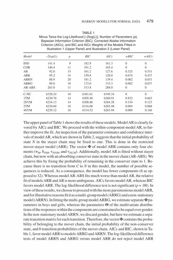
The upper panel of Table 1 shows the results of these models. Model AR is clearly fa-vored by AICc and BIC. We proceed with the within-component model AR, to fur-ther improve the fit. An inspection of the parameter estimates and confidence inter-vals of model AR, which are shown in Table 2, suggests that the initial probability ofstate N in the stayer chain may be fixed to one. This is done in the restrictedmover-stayer model (ARR). The vector � of model ARR contains only four ele-ments (�M, �N|M, �N|NM, and �N|CM). Additionally, model AR is fitted without stayerchain, but now with an absorbing conserver state in the mover chain (AR-ABS). Weachieve this by fixing the probability of remaining in the conserver state to 1. Be-cause there is no transition from C to N in this model, the number of possible se-quences is reduced. As a consequence, the model has fewer components (6 as op-posed to 32). Whereas model AR-ABS fits much worse than model AR, the relativefit of models ARR and AR is more ambiguous. AICc favors model AR, whereas BICfavors model ARR. The log-likelihood difference test is not significant (p = .08). Inviewof these results,wechoose toproceedwith themoreparsimoniousmodelARR,andfor illustrativereasonsfit it asamulti-groupmodel (ARRG)andanon-stationarymodel (ARRN). In fitting the multi-group model ARRG, we estimate separate � pa-rameters in boys and girls, whereas the parameters � of the multivariate distribu-tionsof the responseswithin thecomponentsareconstrained tobeequalovergender.In the non-stationary model ARRN, we discard gender, but here we estimate a sepa-rate transition matrix for each transition. Therefore, the vector � contains the proba-bility of belonging to the mover chain, the initial probability of the non-conserverstate, and 8 transition probabilities of the mover chain. AICc and BIC, shown in Ta-ble 1, favor model ARR to models ARRG and ARRN. The log-likelihood differencetests of model ARRN and ARRG versus model ARR do not reject model ARR


TABLE 1Minus Twice the Log-Likelihood [–2log(L)], Number of Parameters (p),

Bayesian Information Criterion (BIC), Corrected Akaike InformationCriterion (AICc), and BIC and AICc Weights of the Models Fitted in

Illustration 1 (Upper Panel) and Illustration 2 (Lower Panel)

Model –2log(L) p BIC AICc wBIC wAICc

IND 141.4 9 182.9 161.3 0 0COR 140.4 11 191.2 165.4 0 0AR 92.0 15 161.2 127.6 0.325 0.531ARR 95.2 14 159.8 128.0 0.674 0.437ARRN 88.9 20 181.2 139.4 0.002 0.031ARRG 89.0 18 172.0 133.3 0.002 0.037AR-ABS 263.0 11 313.8 288.0 0 0

C-NC 6328.24 10 6381.61 6349.34 0 01TM 6230.76 14 6305.48 6260.91 0.832 0.6632SYM 6234.13 14 6308.86 6264.28 0.154 0.1232TM 6230.66 16 6316.06 6265.48 0.004 0.0684SYM 6229.12 16 6314.52 6263.94 0.009 0.146

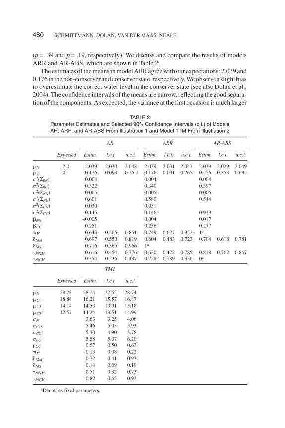
(p = .39 and p = .19, respectively). We discuss and compare the results of modelsARR and AR-ABS, which are shown in Table 2.

The estimates of the means in model ARR agree with our expectations: 2.039 and0.176 in thenon-conserverandconserverstate, respectively.Weobserveaslightbiasto overestimate the correct water level in the conserver state (see also Dolan et al.,2004). The confidence intervals of the means are narrow, reflecting the good separa-tion of the components. As expected, the variance at the first occasion is much larger


TABLE 2Parameter Estimates and Selected 90% Confidence Intervals (c.i.) of ModelsAR, ARR, and AR-ABS From Illustration 1 and Model 1TM From Illustration 2

AR ARR AR-ABS

Expected Estim. l.c.i. u.c.i. Estim. l.c.i. u.c.i. Estim. l.c.i. u.c.i.

�N 2.0 2.039 2.030 2.048 2.039 2.031 2.047 2.039 2.029 2.049�C 0 0.176 0.093 0.265 0.176 0.091 0.265 0.526 0.353 0.695�2(Σ0N) 0.004 0.004 0.004�2(Σ0C) 0.322 0.340 0.397�2(ΣNN) 0.005 0.005 0.006�2(ΣNC) 0.601 0.580 0.544�2(ΣCN) 0.030 0.031�2(ΣCC) 0.145 0.146 0.939 NN –0.005 0.004 0.017 CC 0.251 0.256 0.277�M 0.643 0.505 0.851 0.749 0.627 0.952 1a

�N|M 0.697 0.550 0.819 0.604 0.483 0.723 0.704 0.618 0.781�N|S 0.716 0.365 0.966 1a

�N|NM 0.616 0.454 0.776 0.630 0.472 0.785 0.818 0.762 0.867�N|CM 0.354 0.236 0.487 0.258 0.189 0.336 0a

TM1

Expected Estim. l.c.i. u.c.i.

�N 28.28 28.14 27.52 28.74�C1 18.86 16.21 15.57 16.87�C2 14.14 14.53 13.91 15.18�C3 12.57 14.24 13.51 14.99�N 3.63 3.25 4.06�C15 5.46 5.05 5.93�C24 5.30 4.90 5.78�C3 5.58 5.07 6.20�CC 0.57 0.50 0.63�M 0.13 0.08 0.22�N|M 0.72 0.41 0.93�N|S 0.14 0.09 0.19�N|NM 0.51 0.32 0.73�N|CM 0.82 0.65 0.93

aDenot1es fixed parameters.

in the conserver state, �2(Σ0C) = 0.340, than in the non-conserver state, �2(Σ0N) =0.004. The residual variances associated with the transitions NN, CN and CC aresmall compared to the residualvariancesof the transitionNC.Theautoregressiveco-efficient between two consecutive non-conserver states is small NN = 0.004, com-pared to the autoregressive coefficient between two conserver states CC = 0.256.The residual variances and autoregressive coefficients result in a mean variance inthe non-conserver state (conserver state) of 0.015 (0.368) with a standard deviationof0.013 (0.185). Asexpected, thevariance is larger in theconserver states than in thenon-conserver states.Themeancorrelationbetween twoconsecutivenon-conserverstates is close to zero (0.006), whereas the mean correlation between two consecu-tive conserver states equals 0.361. The probability of belonging to the mover chainequals 0.749. The initial probability of the movers to start in the non-conserver stateequals 0.604. The estimates of the transition probability from non-conserver(conserver) to non-conserver state equals 0.630 (0.258).

In comparing the results of model ARR to those of the poorly fitting modelAR-ABS, it is noteworthy that the mean of the conserver component is much larger(�C = 0.526) than expected, and larger than in all the other models (0.169 < �C <0.303). In addition, the residual variance of remaining in the conserver state ismuch larger (�2(ΣCC) = 0.9392) than in the other simplex models (0.143 < �2(ΣCC)< 0.146). These results reflect the incorporation of the switching components intothe absorbing conserver components, as they have a larger variance than thenon-conserver components. Note that this also can be observed, when a two-com-ponent independent response model (one conserver and one non-conserver-com-ponent, without switching) is fitted to the data (–2logL = 400.9, npar = 5, BIC =424, AICc = 412). The poor fit of model AR-ABS is consistent with the Piagetiantheory, and the experimental finding that the transition from the non-conserver tothe conserver state proceeds via an unstable transition phase (e.g., van der Maas,1993; van der Maas & Molenaar, 1996).

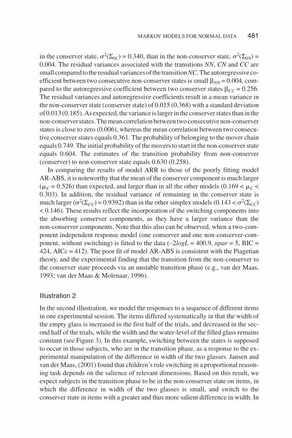
Illustration 2

In the second illustration, we model the responses to a sequence of different itemsin one experimental session. The items differed systematically in that the width ofthe empty glass is increased in the first half of the trials, and decreased in the sec-ond half of the trials, while the width and the water-level of the filled glass remainsconstant (see Figure 3). In this example, switching between the states is supposedto occur in those subjects, who are in the transition phase, as a response to the ex-perimental manipulation of the difference in width of the two glasses. Jansen andvan der Maas, (2001) found that children’s rule switching in a proportional reason-ing task depends on the salience of relevant dimensions. Based on this result, weexpect subjects in the transition phase to be in the non-conserver state on items, inwhich the difference in width of the two glasses is small, and switch to theconserver state in items with a greater and thus more salient difference in width. In


other words, in addition to the stayer chain, we expect a chain, in which subjectsswitch from non-conserver to conserver state within the first part of the series, andswitch back during the last trials.

Here, the focus is on the patterns of the switches in the mover chain, that is, thepossible sequences, because they may distinguish between continuous and discon-tinuousmodelsofdevelopment.Onepattern, calledhysteresis, ispredictedbycatas-trophe theory (a discontinuous model), but not by any continuous model, and there-fore is an important indication of discontinuous development (Jansen & van derMaas, 2001; van der Maas & Molenaar, 1992). In the present example, hysteresis oc-curs when the switch back from conserver to non-conserver state occurs in an itemwith a smaller difference in width than the first switch from the non-conserver stateto the conserver state. It is possible to constrain the transition matrices of the moverchain in such a way that only specific sequences are possible, for example, patternsthatareorarenot inconcordancewith theexistenceofhysteresis.However, as thees-timated number of subjects in the transition phase is small, we consider only a roughimplementation of hysteresis patterns.

Task. The paper-and-pencil hysteresis conservation anticipation task con-sists of nine systematically varying items. As mentioned above, the width of theempty glass is increased in the first five trials, and decreased by the same steps inthe 4 subsequent trials. Each trial is given on a separate page of the test booklet. Weanalyze five trials (Trials 2, 4, 5, 6, and 8), which we refer to as Trials 1 to 5 (seeFigure 3). The items used at Trials 1 and 5 are identical (Item 1), as are the itemsused at Trials 2 and 4 (Item 2). The participants indicated the predicted water levelby drawing a line in the right glass. The mean of the height measured from the bot-tom of the glass at the left and at the right side was recorded in millimeters.

Sample. A total of 208 children in the age range from 5.9 to 8.0 years (mean10.4) completed the hysteresis conservation anticipation task in their school settings(for details, see Jansen & van der Maas, 2001). Only 1% of the data is missing.

Models. We report the results of five models. In all models, a simple covar-iance structure model within the components is adopted, in which the correlationbetween conserver responses is estimated �CC, whereas all other correlations arefixed to zero. As the non-conservers are expected to respond with a simple align-ment, and the water-level of the left glass equals 28.28 mm in all items, we estimatea single mean and variance in the non-conserver state. The correct responses onTrials 1 and 5 and on Trials 2 and 4 are identical. Therefore, we estimate three dif-ferent means and variances in the conserver state. Together, these total nine param-eters. For example, the component mean vector and the component covariance ma-trices of the component that corresponds to the sequence s = NNCCN in these threewithin-component models are:


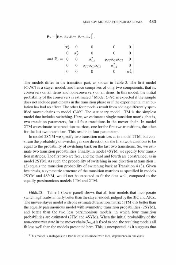
The models differ in the transition part, as shown in Table 3. The first model(C-NC) is a stayer model, and hence comprises of only two components, that is,conservers on all items and non-conservers on all items. In this model, the initialprobability of the conservers is estimated.8 Model C-NC is expected if the sampledoes not include participants in the transition phase or if the experimental manipu-lation has had no effect. The other four models result from adding differently spec-ified mover chains to model C-NC. The stationary model 1TM is the simplestmodel that includes switching. Here, we estimate a single transition matrix, that is,two transition parameters, for all four transitions in the mover chain. In model2TM we estimate two transition matrices, one for the first two transitions, the otherfor the last two transitions. This results in four parameters.

In model 2SYM we specify two transition matrices as in model 2TM, but con-strain the probability of switching in one direction on the first two transitions to beequal to the probability of switching back on the last two transitions. So, we esti-mate two transition probabilities. Finally, in model 4SYM, we specify four transi-tion matrices. The first two are free, and the third and fourth are constrained, as inmodel 2SYM. As such, the probability of switching in one direction at transition 1(2) equals the transition probability of switching back at Transition 4 (3). Givenhysteresis, a symmetric structure of the transition matrices as specified in models2SYM and 4SYM, would not be expected to fit the data well, compared to theequally parsimonious models 1TM and 2TM.

Results. Table 1 (lower panel) shows that all four models that incorporateswitchingfit substantiallybetter than thestayer-model, judgedby theBICandAICc.The mover-stayer model with one estimated transition matrix (1TM) fits better thanthe equally parsimonious model with symmetric transition probabilities (2SYM),and better than the two less parsimonious models, in which four transitionprobabilities are estimated (2TM and 4SYM). When the initial probability of thenon-conserver state in the mover chain (�N|M) is fixed to one, the resulting models allfit less well than the models presented here. This is unexpected, as it suggests that


� �3 2

2

2

23 23

23 2 2

2

, , , , ,

0 0 0 0

0 0 0 0

.0 0 0

0 0 0

0 0 0 0

ts N N C C N

N

N

CC C CC

CC C C C

N

and

� � � � �

�

�

� � � �

� � � �

�

�

�

� �

� �

� �

� ��

� �

� �

� �

� �

� ��

�

�s

8This model is analogous to a two-latent class model with local dependence in one class.

some participants respond correctly on the supposedly more difficult first item, andthen switch to the non-conserver state on later, presumably easier, items.

We focus on the parameter estimates of model 1TM, which are shown togetherwith 90% confidence intervals in Table 2. The mean in the non-conserver state isestimated as �N = 28.140 mm, as expected, and the means in the conserver state are�C1 = 16.21 mm, �C2 = 14.53 mm, �C3 = 14.24 mm. The estimates differ slightlyfrom the expected values, but the means decrease, as expected. The standard devia-tion in the non-conserver state (�N = 3.62) is lower than in the conserver states (�C1

= 5.460, �C2 = 5.300, �C3 = 5.579). The correlation between the responses of twoconserver states equals �CC = 0.566. The proportion of stayers is quite high (�stayer

= 0.872). The proportion of non-conservers is small in the stayer chain (�N|S =0.141). In the mover chain the probability of starting in the non-conserver stateequals �N|M = 0.718, and the transition probabilities equal �N|NM = 0.505 and �C|CM =0. 821. As can be seen in the lower part of Table 2, the 90% confidence intervals ofthe transition parameters in the mover chain are large. This is due to the fact thatthese parameter estimates are based on only a small part of the whole sample, thatis, the number of movers that is estimated as 208 × 0.1281 = 27.

The results suggest that in the present data set the existence of hysteresis is quiteprobable. Unfortunately, as only a small number of the participants is in the transi-tion phase, and as the separation of the components is less good than in the first il-lustration, it is not possible to draw strong conclusions about the existence of hys-


TABLE 3Transition Matrices of the Fitted Models

ModelTransition 1Trial 1 to 2

Transition 2Trial 2 to 3



C-NC

1TM

2TM

2SYM

4SYM

Note. Free parameters are denoted by letters. Parameters denoted by the sameletter are constrained to be equal

�

�

�

�

�

�

�

�

1 1 1 1

1 1 1 1

a b a b a b a b

a b a b a b a b

� � � �

� � � � � � � ��

� � � � � � � �

� � � � � � � �

�

�

�

�

�

�

�

�

1 1 1 1

1 1 1 1

a b a b c d c d

a b a b c d c d

� � � �

� � � � � � � ��

� � � � � � � �

� � � � � � � �

�

�

�

�

�

�

�

�

1 1 1 1

1 1 1 1

a b a b b a b a

a b a b b a b a

� � � �

� � � � � � � ��

� � � � � � � �

� � � � � � � �

�

�

�

�

�

�

�

�

1 1 1 1

1 1 1 1

a b c d d c b a

a b c d d c b a

� � � �

� � � � � � � �

� � � � � � � �

� � � � � � � �

1 0 1 0 1 0 1 0

0 1 0 1 0 1 0 1

� � � �

� � � � � � � ��

� � � � � � � �

� � � � � � � �

teresis. However, with the present models the presence of hysteresis can be testedin further studies, in which the separation of the components should be increasedby improving the test stimuli, and in which more data should be gathered inparticipants who are in the transition phase.

DISCUSSION

In contrast to Markovian transition models for discrete longitudinal data, analogousmodels for normal data have received relatively little attention. Dolan et al. (2004) isan exception, but they considered only a single model (analogous to van de Pol andLangeheine’s, 1990, latent Markov model). In the present article, we have presentedand applied a general model for normal data, which includes the same set of modelsas van de Pol and Langeheine’s MMLC model for discrete data. We discussed anddemonstrated the possibility of combining the Markovian transition model withcovariance structure modeling of individual differences within a given sequence ofclasses. That is, we do not require independence of responses, conditional on class,or on sequence of classes. The possibility of covariance structure modeling allowsone to test substantive hypotheses concerning the psychological processes that areinvolved in producing a given response. Similar possibilities in discrete models havebeen considered by Uebersax (1999) and Hagenaars (1988). However, the LISRELsubmodel considered here generally confers great flexibility, as it includes manyspecific models, such as factor models, simplex models, and random effects models.For example, see Dolan, Schmittmann, Lubke, and Neale (2005) for a simple transi-tion model based on the linear growth curve model.

In addition to presenting the general model, we demonstrated that the variousspecial cases of the general model may be viewed as highly constrained (possiblymulti-group) multivariate normal mixture models (see also Dolan et al., 2004). Assuch, these models can be fitted in the program Mx (Neale & Miller, 1997) bymeans of raw data likelihood estimation. Actual model specification in Mx rangesfrom the simple (e.g., models that include conditional independence, e.g., modelIND above) to the quite complicated. In some cases, we wrote scripts in the freelyavailable program R (R Development Core Team, 2004) to facilitate the Mx speci-fication. These R scripts as well as the Mx input scripts used here are available onrequest. Once the scripts were in place, we encountered few computational prob-lems in running Mx. We did consistently vary starting values, as local minima forma well-known potential problem in mixture modeling (McLachlan & Peel, 2000).Fortunately, Mx has the facility to vary starting values automatically. The feasibil-ity of fitting mixtures depends in part on the separation of the components. Whilethe latent classes were well separated in Illustration 1, they were much less wellseparated in Illustration 2, without causing great computational difficulties. No


doubt, this is due in part to the fact that the mixtures are highly constrained, bothwith respect to the means and the mixing proportions.

Although our aim was to present a version of van de Pol and Langeheine’s(1990) MMLC model for normal data, the present implementation of this model inMx offers several novel possibilities, such as LISREL modeling within a sequenceof classes. In addition, we demonstrated in Illustration 2 the possibility of varyingthe exact nature of the indicator variable. This allows one to experimentally inves-tigate the effects of stimulus manipulation on the transition between latent classes.This offers interesting possibilities in studying learning (e.g., Raijmakers, Dolan,& Molenaar, 2001; Schmittmann, Raijmakers, & Visser, 2005). Of course in vary-ing stimulus material, one has to take care that the nature of the construct beingmeasured does not change. In the case of Illustration 2, we consider this problem tobe negligible (see Figure 3). The possibility of specifying non-stationary transitionprobabilities is useful in combination with varying indicators.

We have limited our presentation to single indicator models, that is, the re-peated measures are univariate. Langeheine (1994) has extended the generalMMLC model (van de Pol & Langeheine, 1990) to include multiple indicators.This same extension in the normal analogue of the MMLC model, presented here,is also possible. For an example of this in the present model, again using Mx, werefer the reader to the Mx script library (see Footnote 2).

REFERENCES

Azzelini, A. (1996). Statistical inference based on the likelihood. London: Chapman and Hall.Bartholomew, D. J., & Knott, M. (1999). Latent variable models and factor analysis (2nd ed.). New

York: Oxford University Press.Bollen, K. A. (1989). Structural equations with latent variables. New York: Wiley.Boom, J., Hoijtink, H., & Kunnen, S. (2001). Rules in the balance: Classes, strategies, or rules for the

balance scale task. Cognitive Development, 16, 717–736.Buckland, S. T., Burnham, K. P., & Augustin, N. H. (1997). Model selection: An integral part of infer-

ence. Biometrics, 53, 603–618.Collins, L. M., Lanza, S. T., Schafer, J. L., & Flaherty, B. P. (2002). WinLTA users guide. Version 3.0

[Computer software manual]. University Park: The Methodology Center, The Pennsylvania StateUniversity.

Collins, L. M., & Wugalter, S. E. (1992). Latent class models for stage-sequential dynamic latent vari-ables. Multivariate Behavioral Research, 27, 131–157.

Dolan,C.V., Jansen,B.R. J.,&vanderMaas,H.L. J. (2004).Constrainedandunconstrainedmultivariatenormal finite mixture modeling of Piagetian data. Multivariate Behavioral Research, 39, 89–98.

Dolan, C. V., Schmittmann, V. D., Lubke, G. H., & Neale, M. C. (2005). Regime switching in the latentgrowth curve mixture model. Structural Equation Modeling, 12, 94–119.

Dolan, C. V., & van der Maas, H. L. J. (1998). Fitting multivariate normal mixtures subject to structuralequation modeling. Psychometrika, 63, 227–253.

Flavell, J. H. (1971). Stage-related properties of cognitive development. Cognitive Psychology, 2,421–453.


Gill, P. E., Murray, W., Saunders, M. A., & Wright, M. H. (1986). User’s guide for NPSOL (version5.0–2). (Technical Rep. No. SOL 86–2. No. CA.94305). Stanford, CA: Department of OperationsResearch, Stanford University.

Hagenaars, J. A. (1988). Latent structure models with direct effects between indicators. SociologicalMethods and Research, 16, 379–405.

Hamilton, J. D. (1994). Time series analysis. Princeton, NJ: Princeton University Press.Hurvich, C. M., & Tsai, C.-L. (1995). Model selection for extended quasi-likelihood models in small

samples. Biometrics, 51, 1077–1084.Jansen, B. R. J., & van der Maas, H. L. J. (2001). Evidence for the phase transition from Rule I to Rule II

on the balance scale task. Developmental Review, 21, 450–494.Jöreskog, K. G. (1970). Estimation and testing of simplex models. The British Journal of Mathematical

and Statistical Psychology, 23, 121–145.Jöreskog, K. G., & Sörbom, D. (2002). LISREL 8: Structural Equation Modeling with the SIMPLIS

command language. Chicago: Scientific Software International.Kemeny, J. G., & Snell, J. L. (1976). Finite Markov chains: With a new appendix ‘Generalization of a

Fundamental Matrix’. New York: Springer-Verlag.Kim, C.-J., & Nelson, C. R. (1999). State-space models with regime switching. Cambridge, MA: MIT

Press.Langeheine, T. (1994). Latent variable Markov models. In A. von Eye & C. C. Clogg (Eds.), Latent

variable analysis. Applications for developmental research. Thousand Oaks, CA: Sage.Lazarsfeld, P. F., & Henry, N. W. (1968). Latent structure analysis. New York: Houghton Mifflin.Little, R. J., & Rubin, D. B. (1989). The analysis of social science data with missing values. Sociologi-

cal Methods and Research, 18, 292–326.McLachlan, G., & Peel, D. (2000). Finite mixture models. New York: Wiley.Muthén, B. O., Kaplan, D., & Hollis, M. (1987). On structural equation modeling with data that are not

missing completely at random. Psychometrika, 52, 431–462.Neale, M. C., Boker, S. M., Xie, G., & Maes, H. H. (2002). Mx: Statistical modeling (6th ed.). VCU,

Richmond, VA: Author.Neale, M. C., & Miller, M. (1997). The use of likelihood-based confidence intervals in genetic models.

Behavior Genetics, 27, 113–120.Piaget, J., & Inhelder, B. (1969). The psychology of the child. New York: Basic Books.Raijmakers, M. E. J., Dolan, C. V., & Molenaar, P. C. M. (2001). Finite mixture distribution models of

simple discrimination learning. Memory and Cognition, 29, 659–677.R Development Core Team. (2004). R: A language and environment for statistical computing (ISBN

3–900051-00–3). Vienna, Austria: R Foundation for Statistical Computing (http://www.R-pro-ject.org).

Reise, S. P., & Duan, N. (2003). Multilevel modeling: Methodological advances, issues, and applica-tions. Mahwah, NJ: Lawrence Erlbaum Associates, Inc.

Schmittmann, V. D., Visser, I., & Raijmakers, M. E. J. (in press). Multiple learning modes in the devel-opment of performance on a rules-based category-learning task. Neuropsychologia.

Schwarz, G. (1978). Estimating the dimension of a model. Annals of Statistics, 6, 461–464.Stewart, A., Phillips, T., & Dempsey, G. (1998). Pharmacotherapy for people with Alzheimer’s disease:

A Markov-cycle evaluation of five years’ therapy using Donepezil. International Journal of Geriat-ric Psychiatry, 13, 445–453.

Thomas, H., & Hettmansperger, T. P. (2001). Modelling change in cognitive understanding with finitemixtures. Applied Statistics, 40, 435–448.

Uebersax, J. S. (1999). Probit Latent class analysis with dochotomous or ordered category measures:Conditional independence/dependence models. Applied Psychological Measurement, 23, 283–297.

van de Pol, F, & Langeheine, R. (1990). Mixed Markov latent class models. Sociological Methodology,20, 213–248.


van de Pol, F., Langeheine, R., & de Jong, W. (1989). PANMARK User’s Manual, PANel analysis usingMARKov chains. Version 1.5. Voorburg: Netherlands Central Bureau of Statistics.

van der Maas, H. L. J.. (1993). Catastrophe analysis of stagewise cognitive development: Model,method and applications. Doctoral dissertation (Dissertatie reeks 1993–2), University of Amster-dam.

van der Maas, H. L. J., & Molenaar, P. C. M. (1992). Stagewise cognitive development: An applicationof catastrophe theory. Psychological Review, 99, 395–417.

van der Maas, H. L. J., & Molenaar, P. C. M. (1996). Catastrophe analysis of discontinuous develop-ment. In A. A. van Eye & C. C. Clogg (Eds.), Categorical variables in developmental research.Methods of analysis (pp. 77–105). San Diego: Academic Press.

Vermunt, J. K. (1997). �EM: A general program for the analysis of categorial data. Tilburg, The Neth-erlands: Author.

Wagenmakers, E. J., & Farrell, S. (2004). AIC model selection using Akaike weights. PsychonomicBulletin and Review, 11, 192–196.

Wickens, T. D. (1982). Models for behavior: Stochastic processes in psychology. San Francisco: W. H.Freeman.

Wolfe, J. H. (1970). Pattern clustering by multivariate mixture analysis. Multivariate Behavioral Re-search, 5, 329–350.

Wolfe, R., Carlin, J. B., & Patton, G. C. (2003). Transitions in an imperfectly observed binary variable:Depressive symptomatology in adolescents. Statistics in Medicine, 22, 427–440.

Wothke, W. (2000). Longitudinal and multi-group modeling with missing data. In T. D. Little, K. U.Schnabel, & J. Baumert (Eds.), Modeling longitudinal and multilevel data: Practical issues, appliedapproaches, and specific examples. Mahwah, NJ: Lawrence Erlbaum Associates, Inc.

Yung, Y. F. (1997). Finite mixtures in confirmatory factor-analysis models. Psychometrika, 62,297–330.

Accepted December 2004


Discrete Latent Markov Models for Normally Distributed Response Data

Documents

Transcript of Discrete Latent Markov Models for Normally Distributed Response Data