A hidden Markov model for predicting protein interfaces

July 11, 2007 22:49 WSPC/185-JBCB 00272

Journal of Bioinformatics and Computational BiologyVol. 5, No. 3 (2007) 739–753c© Imperial College Press

A HIDDEN MARKOV MODEL FOR PREDICTINGPROTEIN INTERFACES

CAO NGUYEN

Department of Computer Science and EngineeringUniversity of Colorado at Denver and Health Sciences

Denver, CO. 80217, [email protected]

KATHELEEN J. GARDINER

Eleanor Roosevelt Institute at the University of Denver andDepartment of Biochemistry and Molecular Genetics

Department of PediatricsUniversity of Colorado at Denver and Health Sciences Center

Denver, CO. 80262, [email protected]

KRZYSZTOF J. CIOS

Department of Computer Science and EngineeringUniversity of Colorado at Denver and Health Sciences Center

Department of Computer Science, University of Colorado at BoulderDepartment of Preventive Medicine and Biometrics

School of Medicine, UCDHSC, and 4cData, LLC Denver, CO. 80217, [email protected]

Received 31 August 2006Revised 26 December 2006

Protein–protein interactions play a defining role in protein function. Identifying the sitesof interaction in a protein is a critical problem for understanding its functional mecha-nisms, as well as for drug design. To predict sites within a protein chain that participatein protein complexes, we have developed a novel method based on the Hidden MarkovModel, which combines several biological characteristics of the sequences neighboring atarget residue: structural information, accessible surface area, and transition probabil-ity among amino acids. We have evaluated the method using 5-fold cross-validation on139 unique proteins and demonstrated precision of 66% and recall of 61% in identify-ing interfaces. These results are better than those achieved by other methods used foridentification of interfaces.

Keywords: Protein–protein interaction; protein interface; support vector machine; hid-den Markov model; protein function; sequence profile.

739

July 11, 2007 22:49 WSPC/185-JBCB 00272

740 C. Nguyen, K. J. Gardiner & K. J. Cios

1. Introduction

The goal of proteomics research is to understand protein functions. Critical toreaching this goal is information regarding protein–protein interactions. Proteininteractions are essential for biological processes that range from the formation ofmacromolecular structures and enzymatic complexes to the regulation of signaltransduction pathways. Protein interfaces are defined as domains for selectiverecognition between molecules and for the formation of complexes. Identification ofthese interfaces is important, not only for understanding protein function but alsofor understanding the effects of mutations and for efficient drug design. Currently,the only reliable method for predicting interfaces requires knowledge of tertiarystructures of protein complexes. However, because such information requires sophis-ticated and expensive NMR and X-ray diffraction studies, only a small fraction ofknown protein sequences have tertiary structures determined. Thus, there is a needto develop predictive methods for identifying interfaces.1

A number of researchers have analyzed features of protein interface sites.Chothia and Janin2 determined that such sites are more hydrophobic, flat orprotruding than other surfaces. Jones and Thornton3 studied properties of pro-tein surfaces surrounding interacting residues and concluded that several physi-cal characteristics, such as Accessible Surface Area (ASA), were very influential.Sheinerman and Honig4 looked at the contribution of electrostatic interactions, thepresence of a significant population of charged and polar residues, on interfaces.Ofran and Rost5 found that amino acid composition and preferences for residue-residue interactions could be used to differentiate six types of protein interfaces,each corresponding to a different functional association between residues.

Based on the features of known protein interfaces, several computational meth-ods have been reported for their prediction. One approach was based on physicaland chemical characteristics of protein interfaces. Jones and Thornton6 predictedinterface patches using the sum of values of solvation, residue interface propensity,hydrophobicity, flatness, protrusion index and ASA. The algorithm by Kini andEvans7 used the fact that proline residues occurred near interfaces at a frequency2.5 times higher than expected by chance. Pazos et al.8 used multiple sequencealignments and correlated mutations based on the hypothesis that residues partic-ipating in functionally required interactions tend to show compensatory mutationsduring evolution. Gallet et al.9 reported that interfaces can be predicted by usingthe hydrophobic moment and averaged hydrophobicity.

Another approach to predict interfaces is to use machine learning methods,such as neural networks, Bayesian statistics and support vector machines (SVM),with sequence profiles and/or ASA as input data. Zhou and Shan10 and Fariselliet al.11 used a neural network to learn whether or not exposed residues at theprotein surface were in a contact patch. Koike and Takagi12 applied SVM to classifyinterfaces of residues for both homo and hetero-dimers. Bradford and Westhead13

combined a support vector machine approach with the previous work of Jonesand Thornton6 to predict protein-protein binding site. Bordner and Abagyan14

July 11, 2007 22:49 WSPC/185-JBCB 00272

A Hidden Markov Model for Predicting Protein Interfaces 741

detected protein interfaces by using a SVM trained on a combination of evolutionaryconservation signals plus local surface properties. Chen and Zhou15 extended theirown previous work10 by developing a consensus method that combined two neuralnetworks consecutively. Yan et al.16 reported a two-stage method in which residueclusters belonging to interfaces were detected through the SVM and then used asinput to a Bayesian network classifier to identify the most likely class, interface ornon-interface, for the target residues.

The above machine learning approaches share a common characteristic: theinput to their models is the encoded identities of n contiguous amino acid residues,corresponding to a window of size-n containing the target residue. Each residuein the window is represented by a 20-dimensional vector whose values are the cor-responding frequencies in sequence profiles of the residue (e.g. in the method ofYan et al., the 20-dimensional vector is a 20-bit vector with 1-bit for each letter-code of the 20 amino acid alphabet). These methods are limited because a largeamount of data is needed for training, and more importantly, because the biologicalrelationships between sequence profiles and interfaces are not well established.

Here, we report a novel approach to the problem of predicting protein interfacesthat takes into account biological characteristics of a target residue and its near-est neighbors. These include structural information, transition probability amongamino acids around the target residue (in both strands from the N-terminal toC-terminal and in the opposite direction), and ASA value. We designed a HiddenMarkov Model (HMM) to combine and reflect all these characteristics. Our methodachieved accuracy of 73%, precision of 66%, recall of 61% and correlation of 0.42,on a 139 member protein dataset using 5-fold cross-validation.

2. Methods

2.1. Material

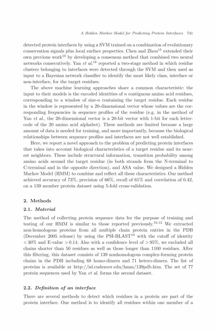
The method of collecting protein sequence data for the purpose of training andtesting of our HMM is similar to those reported previously.10,12 We extractednon-homologous proteins from all multiple chain protein entries in the PDB(December 2005 release) by using the PSI-BLAST19 with the cutoff of identity< 30% and E-value > 0.14. Also with a confidence level of > 95%, we excluded allchains shorter than 50 residues as well as those longer than 1100 residues. Afterthis filtering, this dataset consists of 139 nonhomologous complex-forming proteinchains in the PDB including 68 homo-dimers and 71 hetero-dimers. The list ofproteins is available at http://isl.cudenver.edu/hmm/139pdb.htm. The set of 77protein sequences used by Yan et al. forms the second dataset.

2.2. Definition of an interface

There are several methods to detect which residues in a protein are part of theprotein interface. One method is to identify all residues within one member of a

July 11, 2007 22:49 WSPC/185-JBCB 00272


Fig. 1. Example distribution of interfaces and non-interfaces according to the three categories inthe two datasets, where A is Ambivalent, I is Internal, and E is External.

complex that lie within 5 A of a residue within a second member of the complex.10,12

In this work, we used the definition of Jones and Thornton,3 namely, we calculatedthe difference in the ASA upon complex formation. Using the DSSP program ofKabsch and Sander,20 we extracted the ASA for each residue in the subunits formingthe complex and in the complex. When the ratio of ASA of a residue to its nominalmaximum area in the subunit is at least 25%, the residue is called a surface residue.A surface residue is defined as an interface residue when its calculated ASA valuein the complex is decreased by at least 1 A2. By using this definition, also used inYan et al.,16 we obtained a total of 11 555 interfaces from a total of 33 632 residuesin the 139 protein dataset (see Fig. 1).

2.3. Architecture of the HMM

A first-order discrete HMM is a stochastic generative model for linear problems suchas sequences or time series defined by a finite set D of states, a discrete alphabetS of symbols, a probability transition matrix T = [ti(j)] and a probability emis-sion matrix E = [ek(b)]. Each state k emits symbol b according to E, creating anobservable sequence of symbols. The states are interconnected by state transitionprobabilities T. Starting from an initial state, a sequence of states is generated bymoving from state to state according to the transition probabilities T until the endstate is reached.21

Based on structural information, a protein sequence is reduced from 20-letteramino acid alphabet to three-letter categories of biochemical similarity22: ambiva-lent (Ala, Cys, Gly, Pro, Ser, Thr, Trp, Tyr), external (Arg, Asn, Asp, Gln, Glu,His, Lys), and internal (Ile, Leu, Met, Phe, Val) (see Fig. 1). We observe that, forboth datasets, the fraction of interface proteins in the external category is much

July 11, 2007 22:49 WSPC/185-JBCB 00272


Fig. 2. HMM architecture: there are six inter-connected states plus two fictitious start/end statesusing the three categories. The state designated with a superscript “+” emits symbols located ininterface domains. The emission probability and transition probability parameters are trained byconverted protein sequences in both strands, from N-terminal to C-terminal, and in the oppositedirection.

higher than that in the internal or ambivalent categories (see Fig. 1). This group-ing not only significantly reduces the dimensionality of the input space but it alsoincreases the accuracy of the HMM. For completeness we also show in Table A.1and Fig. 7, in the Appendix, the results obtained by using different HMM models,corresponding to four different monomer groupings based on: (a) chemical, (b) func-tional, (c) charge, and (d) hydrophobic alphabets. In our HMM method, the statesof the class D are defined as D = {A+, E+, I+, A−, E−, I−} and the set of symbolalphabet are defined as S = {A, E, I}, where A stands for ambivalent, E for externaland I for internal (see Fig. 2).

Given the input sequence x = x1x2 · · ·xN with xi ∈ S, we want to find theoutput state sequence π = π1π2 · · ·πN with πi ∈ D such that the probabilityP (x, π|θ) is maximized: π∗ = argmaxπ P (x, π|θ) with the parameters θ are E andT matrices.

2.4. Training of the HMM and making predictions

2.4.1. Training

To train the model the 139 amino-acid letter sequences are first converted intothe three category letter sequences (A, I, E). Next, we use two operators on eachsequence. The expansion operator expands each residue in the three-category-lettersequence into an odd k-residue window containing the residue and �k/2� neighbor-ing residues, on both sides of the residue. It should be noted that when windows i

and i + 1 are connected the last residue of window i and the first residue of win-dow i + 1 are put together, which results in a residue pair. Because this pair doesnot exist in the original sequence it is eliminated from training data. The contrac-tion operator cuts the expanded sequence into connected windows of size m, whereeach window must have in the middle an interface residue, and �m/2� neighboringresidues on either side of the interface. In using the contraction operator the follow-ing rule is applied. Let window i be a window formed with an interface residue in

July 11, 2007 22:49 WSPC/185-JBCB 00272


Fig. 3. Example of transformation from an original sequence into a training sequence that con-stitutes input to the model. In the expansion (with k = 5), the 1st letter A is expanded toAEI (because it has only two residues on the right flank side), the 2nd E is expanded to AEII(because it has one residue on the left and two residues on the right flank side), and the 3rdI is expanded to AEIIA (because it has two residues on both flank sides), and so on. Thetransition between the last residue of window i and the first residue of window i + 1 (markedas ∪) is not used in training task. The contraction operator (with m = 7) cuts: the 1st observedinterface I into a size-7 window NNNI∪NNN; the 2nd observed interface I into a size-7 windowNNNIN∪NN, merged with the previous window (marked as +) to become NNNI∪NNN+IN∪NN;the 3rd observed interface I into N∪NNINI∪N, merged with the previous window (marked as +)to become NNNI∪NNN+IN∪NN+INI∪N. The 4th observed interface I belongs to the previouswindow, thus no window is formed for the 4th interface, and so on.

the middle, then if the next observed interface residue belongs to this window i, thesaid interface residue is omitted, and as a result, no window is formed. Otherwise,window i + 1 is formed with the said interface in the middle and merged with win-dow i (see Fig. 3). These two operators exploit the fact that interface residues tendto form clusters within the amino acid sequence.23 First, the expansion operatorexpands residues around the target residues, and thus improves the transition prob-ability among the amino acids around the target residues. Second, the contractionoperator cuts the expanded sequence into connected windows, where the middleresidue is an interface. Thus, we again focus on clustering of interface residues. Weempirically determined values of k = 5 for the first operator and of m = 7 forthe second. The transformed sequences are input into the model in both strandsfrom the N−terminal to the C−terminal, and in the reverse direction, to learn theemission and transition probabilities, E and T.

2.4.2. Predictions

A protein sequence is converted into the three-category letter sequence before itis used as an input to the model. In this phase, the two operators will not be usedbecause we do not have the knowledge of interfaces of the protein. Then we use

July 11, 2007 22:49 WSPC/185-JBCB 00272


the Viterbi algorithm,21 to find the most probable path of output state sequenceπ = π1π2 · · ·πN . The initial state π1 is chosen according to an initial distributionof the states. Interfaces are residues emitted by those states designated with asuperscript “+”.

2.5. Assessment of predictions

The following four measures are used to assess the performance of our HMMmethod:

Precision, or positive predictive value =TP

TP + FP,

Recall, or sensitivity =TP

TP + FN,

Accuracy =TP + TN

TP + TN + FP + FN,

Matthews correlation coefficient

=TP × TN − FP × FN

√(TP + FN ))(TP + FP)(TN + FP)(TN + FN )

where

— TP = the number of residues predicted to be interfaces that actually are inter-faces (true positives)

— TN = the number of residues predicted not to be interfaces that actually arenot interfaces (true negatives)

— FP = the number of residues predicted to be interfaces that actually are notinterfaces (false positives)

— FN = the number of residues predicted not to be interfaces that actually areinterfaces (false negatives)

The Matthews correlation coefficient (MCC) is always between −1 and +1 andmeasures how well the predicted class labels agree with the actual class labels.A value of the MCC of −1 means complete disagreement, +1, complete agreement,and 0 is considered as a random prediction.17 Accuracy gives the overall evaluationof the estimated probability of correct predictions. In this study, we did not useaccuracy because accuracy is sensitive to the distribution of interface proteins andour data is skewed (the negative class � positive class). Thus if we sacrificed truepositives to predict all examples as negative we could have obtained high accuracyof a classifier.24–26

3. Results and Discussion

3.1. HMM prediction results

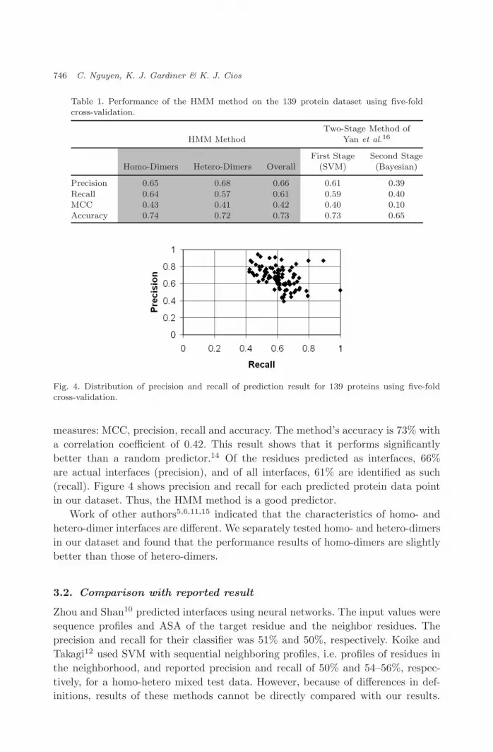
We trained our HMM by using a five-fold cross-validation on the dataset of 139proteins. Table 1 summarizes the results in terms of the following performance

July 11, 2007 22:49 WSPC/185-JBCB 00272


Fig. 4. Distribution of precision and recall of prediction result for 139 proteins using five-foldcross-validation.

measures: MCC, precision, recall and accuracy. The method’s accuracy is 73% witha correlation coefficient of 0.42. This result shows that it performs significantlybetter than a random predictor.14 Of the residues predicted as interfaces, 66%are actual interfaces (precision), and of all interfaces, 61% are identified as such(recall). Figure 4 shows precision and recall for each predicted protein data pointin our dataset. Thus, the HMM method is a good predictor.

Work of other authors5,6,11,15 indicated that the characteristics of homo- andhetero-dimer interfaces are different. We separately tested homo- and hetero-dimersin our dataset and found that the performance results of homo-dimers are slightlybetter than those of hetero-dimers.

3.2. Comparison with reported result

Zhou and Shan10 predicted interfaces using neural networks. The input values weresequence profiles and ASA of the target residue and the neighbor residues. Theprecision and recall for their classifier was 51% and 50%, respectively. Koike andTakagi12 used SVM with sequential neighboring profiles, i.e. profiles of residues inthe neighborhood, and reported precision and recall of 50% and 54–56%, respec-tively, for a homo-hetero mixed test data. However, because of differences in def-initions, results of these methods cannot be directly compared with our results.

July 11, 2007 22:49 WSPC/185-JBCB 00272


For direct comparison, we therefore tested our HMM method on the 77 proteindataset reported by Yan et al.16 We selected Yan et al.’s method for comparisonbecause it used open source SVM and Bayesian network implementations,18 andthus was easy to replicate. To the best of our knowledge, the two-stage classifiermethod of Yan et al. has given the best results so far. Using exactly the same defi-nition to extract the interfaces, we evaluated the two-stage classifier method of Yanet al. using five-fold cross-validation on our 139 protein dataset.

3.2.1. HMM comparison with the two-stage classifier on 139-protein dataset

To evaluate the method of Yan et al. on our 139 protein dataset, we follow theirprocedure and use open-source SVM and Bayesian function implementations. Theinput to the SVM consists of the encoded identities of nine amino acid residuesconsisting of the target residue and the four residues on each side. Each residue inthe window is represented by a 20-bit vector, with 1-bit for each letter representingthe 20 amino acids. Thus, each input data point is of dimension 9 × 20 plus classattribute (1 = interaction site, 0 = noninteraction site). The results are shown inTable 1. They indicate that, in terms of precision, recall and MCC, the performancemeasures of our HMM are slightly better than the SVM used in the first stage.

Next, we evaluate the SVM method by using a different way of encodingresidues.10,12 Each residue in the window, instead of association only with nearestneighbor information, as in the method of Yan et al., is now coded as a 20-dimensionalvector, with its components corresponding to frequencies in the multiple sequencealignment of the protein, taken from the HSSP file.27 When using these input vectors,the SVM’s performance is 58% precision, 38% recall, and 0.27 MCC. These values areworse than using only the nearest-neighbor information as input. Thus, the biologicalrelationships between sequence profiles and interfaces are still questionable.

In the second stage, to compare with the method of Yan et al., a Bayesiannetwork classifier is trained to identify an interaction site residue based on the classlabels (1 = interface, 0 = non-interface) of its neighbors. The class label outputsof the SVM in the first stage constitute input to the Bayesian classifier in thesecond stage. Table 1 shows the results of the second stage using BayesNetB fromthe Weka package,18 with the input being the class labels z of the eight residuessurrounding a target residue, four on each side. The method of Yan et al. classifiesthe target residue as an interface if p(1|z) > λ · p(0|z), where λ ranges from 0.01to 1, in increments of 0.01, so as to maximize the correlation coefficient. The HMMperformed better on the original 139 proteins than the method of Yan et al. usingall measures.

3.2.2. HMM comparison with two-stage classifier on 77-protein dataset

To compare Yan et al.’s method, we use their datasets (77 proteins) and results.The results in Table 2 shows that our HMM method achieves higher recall (53%)than the two-stage method of Yan et al. (39%) when tested on their 77-protein

July 11, 2007 22:49 WSPC/185-JBCB 00272


©

dataset, while the other performance measures are equal. Also, the performancemeasures of the HMM method are significantly better than the method of Galletet al.9 (we use results provided by the authors) when tested on the same dataset. Allsupplementary materials, including the HMM program and datasets, are availableat our web site at http://isl.cudenver.edu/hmm.

4. Conclusions

On the dataset of 139 proteins, our six-state HMM method achieved 73% accuracy,66% precision, 61% recall, and Matthews correlation coefficient of 0.42. Resultsof other HMM variations we designed are shown in Table A.1. In Fig. 5 we illus-trate the performance of the six-state HMM method in terms of tertiary structureof two complexes: the PDB 1BM9 and 1EFN. In several comparisons, our methodperformed better than the two-stage method of Yan et al. on their dataset of 77 pro-teins, as well as when testing their method on our 139 proteins dataset. We have alsoshown that if we use sequence profiles to encode the residues,10,12 the performanceof the SVM method substantially decreases. This suggests that the HMM methodmight be used for predicting effects of point mutations on protein interactions, orsolvent accessibility, from protein sequences.

Validation with the CAPRI targets

Critical Assessment of Prediction of Interactions (CAPRI: http://capri.ebi.ac.uk)is a community wide experiment to assess the capacity of protein docking algo-rithms on targets based on structures of the unbound components. To evaluate ourmethod, we trained the HMM by using the 139 protein dataset and used the result-ing classifier to identify the protein interfaces on the targets. The prediction of theligand HEMK in the target 20 (protein Methyltransferase HEMK complexed withRelease Factor 1, hetero-dimer) is shown in Fig. 6. The HMM identified 32 inter-faces out of 59 positive class residues and 132 non-interfaces out of 217 negativeclass residues.

July 11, 2007 22:49 WSPC/185-JBCB 00272


(a) (b)

Fig. 5. Overall view of complexes with identified interfaces. The predicted protein in each complexis shown in space-fill coded as: Blue: interfaces classified correctly (TPs), Yellow: residues incor-rectly classified as interfaces (FPs), Green: non-interfaces correctly identified as such (TNs), Red:residues incorrectly identified as non-interfaces (FNs); binding proteins are shown as wire-frames:(a) 1BM9 (replication terminator protein from Bacillus Subtilis) (homo-dimer): the predicted pro-tein (chain A), the binding protein (chain B) (b) 1EFN (HIV-1 NEF protein in complex with R96imutant FYN SH3 domain) (hetero-dimer): the predicted protein (chain B), the binding protein(chains A, C, D). The HMM identifies more interfaces in the homo-dimer. The figures were createdusing RasMol (http://www.openrasmol.org).

Fig. 6. Overall view of the ligand HEMK in the target 20 (hetero-dimer) with identified inter-faces. The residues of interest are shown in space-fill coded as: blue, TPs; yellow, FPs; green,TNs; red, FNs; binding proteins are shown as wire-frames. The figure was created using RasMol(http://www.openrasmol.org).

July 11, 2007 22:49 WSPC/185-JBCB 00272


Fig. 7. HMM architectures for monomer grouping based on: (a) Chemical alphabet: there are six-teen inter-connected states (A+, L+, M+, R+, B+, H+, I+, S+, A−, L−,M−, R−, B−, H−, I−, S−)plus two fictitious start/end states according to the eight categories. (b) Functional alpha-bet: there are six inter-connected states (A+, H+, P+, A−, H−, P−) plus two fictitious start/endstates according to the three categories. (c) Charge alphabet: there are four inter-connectedstates (A+, N+, A−, N−) plus two fictitious start/end states according to the two categories.(d) Hydrophobic alphabet: there are four inter-connected states (H+, P+, H−, P−) plus two fic-titious start/end states according to the two categories. The state designated with a superscript“+” emits symbols located in interface domains. The emission probability and transition proba-bility parameters are trained by converted protein sequences in both strands, from N-terminal toC-terminal, and in the opposite direction.

July 11, 2007 22:49 WSPC/185-JBCB 00272


Acknowledgments

The authors acknowledge support from the Vietnamese Ministry of Education andTraining (CN), the National Institutes of Health (HD047671 and HD49460) (KG),and the Butcher Foundation (KJC and CN).

Appendix

Table A.1. Results of the HMM method when monomers are grouped by:

77 Proteins 139 Proteins

(1) Chemical alphabet : (A) acidic (Asp, Glu), (L) aliphatic (Ala, Gly, Ile, Leu, Val), (M)amide (Asn, Gln), (R) aromatic (Phe, Trp, Tyr), (B) basic (Arg, His, Lys), (H) hydroxyl(Ser, Thr), (I) imino (Pro), (S) sulfur (Cys, Met)

Precision 0.53 0.66Recall 0.51 0.61MCC 0.24 0.42

(2) Functional alphabet : (A) acidic and basic (Asp, Glu, Arg, His, Lys), (H) hydrophobic non-polar (Ala, Ile, Leu, Met, Phe, Pro, Trp, Val), (P ) polar uncharged (Asn, Gln, Ser, Thr, Pro,Cys, Met)


(3) Charge alphabet : (A) acidic and basic (Asp, Glu, Arg, His, Lys), (N) neutral (Ala, Ile, Leu,Met, Phe, Pro, Trp, Val, Asn, Gln, Ser, Thr, Pro, Cys, Met)


(4) Hydrophobic alphabet : (H) hydrophobic (Ala, Ile, Leu, Met, Phe, Pro, Trp, Val), (P )hydrophilic (Arg, Asn, Asp, Cys, Gln, Glu, Gly, His, Lys, Ser, Thr, Tyr)


References

1. Valencia A, Pazos F, Computational methods for prediction of protein interactions,Curr Opin Struct Biol 12:368–373, 2002.

2. Chothia C, Janin J, Principles of protein-protein recognition, Nature 256:705–708,1975.

3. Jones S, Thornton JM, Principles of protein–protein interaction, Proc Natl Acad SciUSA 93:13–20, 1996.

4. Sheinerman FB, Honig B, On the role of electrostatic interactions in the design ofprotein–protein interfaces, J Mol Biol 318:161–177, 2002.

5. Ofran Y, Rost B, Analysing six types of protein–protein interfaces, J Mol Biol325:377–387, 2003.

July 11, 2007 22:49 WSPC/185-JBCB 00272


6. Jones S, Thornton JM, Prediction of protein–protein interaction sites using patchanalysis, J Mol Biol 272:133–143, 1997.

7. Kini RM, Evans HJ, Prediction of potential protein–protein interaction sites fromamino acid sequence identification of a fibrin polymerization site, FEBS letters385:81–86, 1996.

8. Pazos F, Helmer-Citterich M, Ausiello G, Valencia A, Correlated mutations containinformation about protein–protein interaction, J Mol Biol 271:511–523, 1997.

9. Gallet X, Charloteaux B, Thomas A, Brasseur R, A fast method to predict proteininteraction sites from sequences, J Mol Biol 302:917–926, 2000.

10. Zhou H, Shan Y, Prediction of protein interaction sites from sequence profile andresidue neighbor list, Proteins 44:336–343, 2001.

11. Fariselli P, Pazos F, Valencia A, Casadi R, Prediction of protein-protein interactionsites in heterocomplexes with neural networks, Eur J Bio-Chem 269:1356–1361, 2002.

12. Koike A, Takagi T, Prediction of protein–protein interaction sites using support vectormachines, Protein Engineering, Design & Selection 17:165–173, 2004.

13. Bradford J, Westhead D, Improved prediction of protein–protein binding sites usinga support vector machines approach, Bioinformatics 21(8):1487–1494, 2005.

14. Bordner A, Abagyan R, Statistical analysis and prediction of protein–protein inter-faces, Proteins: Structure, Function, and Bioinformatics 60(3):353–366, 2005.

15. Chen H, Zhou H, Prediction of interface residues in protein–protein complexes bya consensus neural network method: Test against NMR data, Proteins: Structure,Function, and Bioinformatics 61:21–35, 2005.

16. Yan C, Dobbs D, Honavar V, A two-stage classifier for identification of protein-proteininterface residues, Bioinformatics 20:371i–378i, 2004.

17. Baldi P, Brunak S, Chauvin Y, Andersen F, Assessing the accuracy of predictionalgorithms for classification: An overview, Bioinformatics 16:412–424, 2000.

18. Witten I, Frank E, Data Mining: Practical Machine Learning Tools and Techniques,Morgan Kaufmann, 2005.

19. Altschul SF, Madden TL, Schaffer AA, Zhang J, Zhang Z, Miller W, Lipman DJ,Gapped BLAST and PSI-BLAST: A new generation of protein database search pro-grams, Nucleic Acids Res 25:3389–3402, 1997.

20. Kabsch W, Sander C, Dictionary of protein secondary structure: Pattern recognitionof hydrogen-bonded and geometrical features, Biopolymers 22:2577–2637, 1983.

21. Baldi P, Brunak S, Bioinformatics: The Machine Learning Approach, The MIT Press,2001.

22. Karlin S, Ost F, Blaisdell BE, Patterns in DNA and amino acid sequences andtheir statistical significance, Waterman MS (ed.), in Mathematical Methods for DNASequences, CRC Press, pp. 133–157, 1989.

23. Ofran Y, Rost B, Predicted protein–protein interaction sites from local sequence infor-mation, FEBS Lett 544:236–239, 2003.

24. Cios KJ, Pedrycz W, Swiniarski R, Data Mining Methods for Knowledge Discovery,Kluwer Academic Publishers, 1998.

25. Cios KJ, Kurgan L, CLIP4: Hybrid inductive machine learning algorithm that gen-erates inequality rules, Information Sciences 163:37–83, 2004.

26. Kurgan L, Cios KJ, Scott D, Highly scalable and robust rule learner: Performanceevaluation and comparison, IEEE Transactions on Systems Man and Cybernetics,Part B 36:32–53, 2006.

27. Dodge C, Schneider R, Sander C, The HSSP database of protein structure-sequencealignments and family profiles, Nucleic Acids Res 26(1):313–315, 1998.

July 11, 2007 22:49 WSPC/185-JBCB 00272


Cao Nguyen is a PhD student in Computer Science and Infor-mation Systems program, with the option in ComputationalBiology, at the University of Colorado at Denver and HealthSciences Center (UCDHSC). He conducts research with Dr. Ciosin the area of mathematical modeling (hidden Markov models,clustering, and fuzzy cognitive maps) for prediction of protein–protein interfaces and protein functions. Nguyen holds an MSdegree in Computer Science from the Vietnam National Univer-sity. He has been awarded full scholarship for his study in theU.S.A.

Katheleen J. Gardiner received her PhD degree from the University of Coloradoand is currently a Professor at the Eleanor Roosevelt Institute at the University ofDenver and an Adjoint Associate Professor in the Department of Biochemistry andMolecular Genetics at the UCDHSC. Dr. Gardiner is an internationally recognizedresearcher in the field of Down syndrome. Her specific research interests are inthe identification of genes encoded by human chromosome 21 that contribute tolearning and memory deficits in Down syndrome and the use of data from mouseand other model organisms to predict associated pathway perturbations. She hasauthored over 100 journal articles, meeting reports, and book chapters. Her researchis currently funded by the National Institutes of Health and the Fondation JeromeLejeune.

Krzysztof J. Cios received his MS and PhD degrees from theAGH University of Science and Technology, Krakow, the MBAdegree from the University of Toledo, Ohio, and the DSc degreefrom the Polish Academy of Sciences. He is currently a Profes-sor at the University of Colorado at Denver and Health SciencesCenter, and Associate Director of the University of ColoradoBioenergetics Institute. He directs Data Mining and Bioinfor-matics Laboratory. Dr. Cios is a well-known researcher in the

areas of learning algorithms, biomedical informatics and data mining. NASA, NSF,American Heart Association, Ohio Aerospace Institute, NATO, US Air Force andNIH have funded his research. He published 3 books, about 150 journal and confer-ence articles and 12 book chapters; serves on editorial boards of Neurocomputing,Journal of Integrative Neuroscience, IEEE Engineering in Medicine and BiologyMagazine, International Journal of Computational Intelligence, and Biodata Min-ing; edited 5 special issues of journals. Dr. Cios has been the recipient of the Nor-bert Wiener Outstanding Paper Award, the Neurocomputing Best Paper Award,the University of Toledo Outstanding Faculty Research Award, and the FulbrightSenior Scholar Award. Dr. Cios is a Foreign Member of the Polish Academy of Artsand Sciences.

A hidden Markov model for predicting protein interfaces

Documents

Transcript of A hidden Markov model for predicting protein interfaces