arX

iv:0

808.

2833

v4 [

cs.IT

] 10

Aug

201

0

Efficient Tests for Equivalence of Hidden MarkovProcesses and Quantum Random Walks

Ulrich Faigle1 and Alexander Schonhuth2, Member IEEE

1 Mathematical InstituteCenter for Applied Computer Science

University of CologneWeyertal 80

50931 Koln, Germany2 Department of Mathematics

University of California, Berkeley970 Evans Hall # 3840

Berkeley, CA 94720-3840, USAalexsch@math.berkeley.edu

Abstract. While two hidden Markov process (HMP) resp. quantum ran-dom walk (QRW) parametrizations can differ from one another, the stochas-tic processes arising from them can be equivalent. Here a polynomial-time algorithm is presented which can determine equivalence of two HMPparametrizationsM1,M2 resp. two QRW parametrizationsQ1,Q2 in timeO(|Σ|max(N1, N2)

4), where N1, N2 are the number of hidden states inM1,M2 resp. the dimension of the state spaces associated withQ1,Q2, andΣis the set of output symbols. Previously available algorithms for testing equiva-lence of HMPs were exponential in the number of hidden states. In case of QRWs,algorithms for testing equivalence had not yet been presented. The core subrou-tines of this algorithm can also be used to efficiently test hidden Markov processesand quantum random walks for ergodicity.

Keywords. Dimension, Discrete Random Sources, Hidden Markov Processes,Identifiability, Linearly Dependent Processes, Quantum Random Walks,

1 Introduction

Let a parameterized class of stochastic processes be described by a mapping

Φ : P → S (1)

whereP is the set of parameterizations andS is the corresponding set of stochasticprocesses. A stochastic processΦ(P ) as induced by the parameterizationP is said tobe identifiableiff

Φ−1(Φ(P )) = {P} (2)

that is, iff the parameterization giving rise to it is uniquely determined. The entire classof stochastic processesΦ(P) is said to beidentifiableiff Φ : P → Φ(P) is one-to-one. Theequivalence problem(EP) emerges whenΦ is many-to-one and is to decide

2 U.Faigle/A. Schonhuth

whether two parameterizationsP1, P2 are equivalent, that isΦ(P1) = Φ(P2). Under-standing its solutions can significantly foster understanding of the classes of stochasticprocesses under consideration as it usually yields insights about the class’ complexityand its number of free parameters. Therefore, apart from itstheoretical relevance, it isan important issue in the practice of system identification (e.g. [18]).

Hidden Markov processes (HMPs)are a class of processes which have gainedwidespread attention. In practical applications, for example, they have establishedgold standards in speech recognition and certain areas of computational biology. Seee.g. [19,6,7] for comprehensive related literature. In an intuitive description, a hiddenMarkov process is governed by a Markov process which, however, cannot be observed.Observed symbols are emitted according to another set of distributions which govern thehidden, non-observed states. Since observed processes cancoincide although the non-observed processes on the hidden states can differ from one another, hidden Markovprocesses are non-identifiable.

For hidden Markov processes, the EP was first discussed in 1957 [3] (see also[11] for a subsequent contribution). It was formulated for finite functions of Markovchains (FFMCs), an alternative way of parametrizing hiddenMarkov processes where,as sets of parametrizations, the parametrizations discussed here, also referred to ashid-den Markov models (HMMs)in the following, models trivially contain FFMCs. The EPfor hidden Markov processes was fully solved in 1992 [13]. The corresponding algo-rithm is exponential in the number of hidden states and therefore impractical for largermodels. See [13] also for more related work.

Quantum random walks (QRWs)have been introduced to quantum information the-ory as an analog of classical Markov sources [1]. For example, they allow emulationof Markov Chain Monte Carlo approaches on quantum computers. A collection of re-sults has pointed out that they would be superior to their classical counterparts withrespect to a variety of aspects (see e.g. [15,2,16]). However, although their mechanismscan be described in terms of elementary linear algebraic definitions, their properties aremuch less understood. The key element of a quantum random walk parametrization isa graph whose vertices are the observed symbols. Quantum probability distributions onthe vertices are transformed by linear operations which describe the quantum mechani-cal concepts of evolution and measurement. It is easy to see that quantum random walksare non-identifiable. For example, any of the (infinitely many different) parametriza-tions with a graph of only one vertex yields the same, trivialprocess. The equivalenceproblem for quantum random walks has not been discussed before.

Beyond the work cited in [13], there is a polynomial-time solution to test equiva-lence of probabilistic automata [21] where HMMs can be viewed as probabilistic au-tomata with no final probabilities [5]. The crucial difference, however, is that probabilis-tic automata do not give rise to stochastic processes (distributions over infinite-lengthsequences), but to probability distributions over the set of strings of finite length. Thealgorithm presented in [21] decisively depends on this and therefore does neither applyfor hidden Markov processes nor for quantum random walks. Conversely, by adding astop symbol to the set of observed symbols, any probability distribution over the setof strings of finite length can be viewed as a probability distribution over the set ofinfinite-length symbol sequences. This way, it can be seen that our solution also applies

Efficient Equivalence Tests 3

for probabilistic automata and therefore is more general than [21]’s solution.

Overall, the purpose of this work is to present a simple, polynomial-time algorithmthat solves the EP for both hidden Markov processes and quantum random walks:

Theorem 1. LetΣ be a finite set of symbols and

MX ,MY resp. QX ,QY (3)

be two hidden Markov process resp. quantum random walk parametrizations giving riseto the processes(Xt), (Yt) emitting symbols fromΣ. Let

nX , nY (4)

be the cardinalities of the set of hidden states in the hiddenMarkov models resp. thedimensions of the state spaces associated with the quantum random walks. Equivalenceof (Xt), (Yt) can be determined in

O(|Σ|max{nX , nY }4) (5)

arithmetic operations.

Remark 1.Note that a polynomial-time solution for the identifiability problem forHMPs does not provide a polynomial-time solution for the graph isomorphism prob-lem. There are both non-equivalent HMPs which act on sets of hidden states whichare isomorphic as graphs (e.g. two HMPs both acting on only one hidden state which,however, have different emission probability distributions) and equivalent HMPs whereunderlying graphs are non-ismorphic (e.g. two HMPs, one acting on two hidden states,but emitting the symbola with probability1 from both states and the other one actingon only one hidden state, also emitting the symbola with probability1, both result inthe stochastic process which generatesaaaa.... with probability1).

Remark 2.In [20] it was described how to test HMPs for ergodicity. Plugging the al-gorithm for computation of a basis (see subsection 5.1) intothe generic ergodicity testsprovided in [20] renders these tests efficient.

1.1 Organization of Sections

The core ideas of this work are tightly interconnected with the theory offinitary pro-cesses. Therefore, we start by concisely revisiting their theory in section 2. We thenintroduce hidden Markov models and quantum random walk parametrizations and themechanisms which give rise to the associated processes in section 3. In section 4 weoutline how to most efficiently compute probabilities for both hidden Markov processesand quantum random walks. The algorithm and theorems behindour efficient equiva-lence tests are then presented in section 5. We finally outline some complementaryapplications of our algorithms and make some conclusive remarks.

4 U.Faigle/A. Schonhuth

2 Finitary Random Processes

Throughout this paper, we consider discrete random processes(Xt) that take values inthe (fixed) finite alphabetΣ. We assume that the process emits theempty word� attime t = 0. We denote theprobability functionp of (Xt) by

p(a1 . . . at) := Pr{X1 = a1, . . . , Xt = at} (a1 . . . at ∈ Σt). (6)

As usual, we setΣ∗ :=

⋃

t≥0

Σt (with Σ0 = {�}) (7)

and note thatΣ∗ is a semigroup under the concatenationwv ∈ Σs+t for w ∈ Σs andv ∈ Σt. |v| = ℓ is thelengthof a wordv ∈ Σℓ.

For anyv, w ∈ Σ∗, we define functionspv, pw : Σ∗ → R via

pv(w) := p(wv) =: pw(v) (8)

and viewRΣ∗

as a vector space.p(v = v1...vt|w = w1...ws) generally denotes theconditional probability

p(v|w) := Pr(Xs+1 = v1, ..., Xt+s = vt |X1 = w1, ..., Xs = ws)

=

p(v) if w = �

0 if p(w) = 0p(wv)/p(w) otherwise.

(9)

Furthermore, the subspace

R(p) := span{pv | v ∈ Σ∗} resp. C(p) := span{pw | w ∈ Σ∗} (10)

is therow spaceresp.column spaceassociated with the (probability functionp of) therandom process(Xt).

It is easy to see thatR(p) andC(p) have the same vector space dimension. So wedefine thedimensionof (Xt) (or its probability functionp) as the parameter

dim(Xt) = dim(p) := dimR(p) = dim C(p) ∈ Z+ ∪ {∞}. (11)

For anyI, J ⊆ Σ∗, we define the matrix

PIJ := [p(wv)]v∈I,w∈J ∈ RI×J . (12)

PIJ is calledgeneratingif rk (PIJ) = rk (PΣ∗,Σ∗)(= dim(p)) andbasic if it is gen-erating and minimal among the generatingPIJ , that is |I| = |J | = dim(p) in caseof dim(p) < ∞. In that sense, we call (in slight abuse of language)I resp.J a rowresp.column generator/basisand the pair(IJ) a generator/basisfor p.

We call a process(Xt) finitary if it admits a (finite) basis. So the finitary processesare exactly the ones with finite dimension.

Efficient Equivalence Tests 5

Remark 3.The dimension of a random process is known as itsminimum degree offreedom. The termfinitary was introduced in [12]. Finitary processes are also calledlinearly dependent[14].

Theorem 2. Let (Xt) and (Yt) be discrete, finitary random processes (overΣ) withprobability functionsp andq. Let furthermore(IJ) be a basis for(Xt). Then the fol-lowing statements are equivalent:

(a) p = q.(b) (I, J) is a basis for(Yt) and the equalities

p(v) = q(v), p(wv) = q(wv) and p(wav) = q(wav) (13)

hold for all choices ofv ∈ I, w ∈ J anda ∈ Σ.

Proof. Given a basic matrixPIJ together with the probabilitiesp(v), p(wav) forall v ∈ I, w ∈ J, a ∈ Σ, one can reconstructp via a ”minimal representation” (see,e.g., [13,14,20] for details). ⋄

3 Parametrizations and The Equivalence Problem

3.1 Hidden Markov Processes

A hidden Markov process (HMP)is parametrized by a tupleM = (S,E, π,M) where

1. S = {s1, . . . , sn} is a finite set of“hidden” states2. E = [esa] ∈ RS×Σ is a non-negativeemission probability matrixwith unit row

sums∑

a∈Σ Esa = 1, (i.e. the row vectors ofE are probability distributions onΣ)3. π is aninitial probability distributiononS and4. M = [mij ] ∈ RS×S is a non-negativetransition probability matrixwith unit row

sums∑n

i=1mij = 1 (i.e. the row vectors ofM are probability distributions onS

The associated process(Xt) initially moves to a states ∈ S with probabilityπs andemits the symbolX1 = a with probabilityEsa. Then it moves froms to a states′ withprobabilitymss′ and emits the symbolX2 = a′ with probabilityes′a′ and so on. In thefollowing, we also refer to a parametrizationM = (S,E, π,M) as ahidden Markovmodel (HMM).

3.2 Quantum Random Walks

A quantum random walk (QRW)is parametrized by a tupleQ = (G,U, ψ0) where

1. G = (Σ,E) is a directed,K-regular graph over the alphabetΣ2. U : Ck → Ck is a unitaryevolutionoperator wherek := |E| = K · |Σ| and3. ψ0 ∈ Ck is a wave function, that is||ψ0|| = 1 (||.|| the Euclidean norm).

6 U.Faigle/A. Schonhuth

Edges are labeled by tuples(a, x), a ∈ Σ, x ∈ X whereX is a finite set with|X | = k.Correspondingly,Ck is considered to be spanned by the orthonormal basis

〈 e(a,x) | (a, x) ∈ E 〉.

According to [1] some more specific conditions must hold which do not affect our con-siderations here.

The quantum random walk(Xt) arising from a parametrizationQ = (G,U, ψ0)proceeds by first applying the unitary operatorU toψ0 and subsequently, with probabil-ity

∑

x∈X |(Uψ0)(a,x)|2, “collapsing” (i.e. projecting and renormalizing, which mod-

els a quantum mechanical measurement)Uψ0 to the subspace spanned by the vectorse(a,x),x∈X to generate the first symbolX1 = a. CollapsingUψ0 results in a new wavefunctionψ1. ApplyingU toψ1 and collapsing it, with probability

∑

x∈X |(Uψ1)(a′,x)|2,

to the subspace spanned bye(a′,x),x∈X generates the next symbolX2 = a′. Iterativeapplication ofU and subsequent collapsing generates further symbols.

3.3 The Equivalence Problem

Theequivalence problemcan be framed as follows:

Equivalence Problem (IP)

Given two hidden Markov modelsMX ,MY or two quantum random walk parametriza-tionsQX ,QY , decide whether the associated processes(Xt) and(Yt) are equivalent.

The equivalence problem can, of course, be solved in principle, in the spirit of The-orem 2. In order to efficiently solve it in practice, it suffices to be able to efficientlycompute the following quantities:

(1) A basis(I, J) for the finitary processes(Xt), (Yt) from their parametrizationsMX ,MY .

(2) The corresponding probabilitiesp(v), p(wv), p(wav) for all choices ofv ∈ I, w ∈J, a ∈ Σ.

4 Computing Probabilities

We would like to point out that in the following we assume thatall inputs consist ofrational numbers and that each arithmetic operation can be done in constant time. Thisagrees with the usual conventions when treating related probabilistic concepts in termsof algorithmic complexity [19,21,5].

Efficient Equivalence Tests 7

4.1 Hidden Markov Processes

Let now (Xt) be a hidden Markov process with parametrizationM = (S,E, π,M).Observe first that thetransition matrixM decomposes asM =

∑

a∈Σ Ta into matricesTa with coefficients

(Ta)ij := esia ·mij (14)

which reflect the probabilities to emit symbola from statesi and subsequently to moveon to statesj . Standard technical computations (e.g.[8]) reveal that that for any worda1 . . . at ∈ Σt:

p(a1a2 . . . at) = p(a1a2 . . . at−1)p(at|a1a2 . . . at−1)

= · · ·

= πTTa1 . . . Tat−1Tat1,

(15)

where1 = (1, ..., 1)T ∈ RS is the vector of all ones.

For further reference, we use the notations

Tv := Tv1Tv2 . . . Tvt−1Tvt ∈ Rn×n (16)

for anyv = v1 . . . vt ∈ Σ∗ as well as

−→p (v) := πTTv ∈ R1×n and ←−p (v) := Tv1 ∈ Rn×1. (17)

Remark 4.Note that computation of vectors−→p (v) and←−p (v) is an alternative way todescribe the well-known Forward and Backward algorithm (e.g.[7]) since the entriesof these two vectors can be identified with the Forward and Backward variables

Pr(Ss+1 = si |X1 = a1, ..., Xs = as) (18)

and (19)

Pr(Ss+1 = si |Xs+1 = as+1, ..., Xs+t = as+t) (20)

where(St) is the (non-observable)Markov process over the hidden statesS = (s1, ..., sn).

4.2 Quantum Random Walks

The following considerations can be straightforwardly derived from standard quantummechanical arguments, see [4] for a reference.

The State SpaceSn We writeQ∗ for the adjoint of an arbitrarily sized matrixQ ∈Cm×n, (that isQ∗

ji = a− ib if Qji = a+ ib where usage ofi as both a running indexand a complex number should not lead to confusion). Let

n := k2 = |E|2. (21)

8 U.Faigle/A. Schonhuth

We will consider the set of self-adjoint matrices

Sn := {Q ∈ Ck2

|Q = Q∗} (22)

in the following, which is usually referred to asstate spacein quantum mechanics.As usual,Sn can be viewed as ann = k2-dimensional real-valued vector space. Toillustrate this let

em := (0, ..., 0, 1m, 0, ..., 0)T ∈ CK ,m = 1, ..., k and (23)

fm := (0, ..., 0, im, 0, ..., 0)T ∈ CK ,m = 1, ..., k. (24)

The self-adjoint matrices

Em1m2:= (em1

e∗m2+ em2

e∗m1) and Fm1m2

:= (fm1f∗m2

+ fm2f∗m1

) (25)

for all choices of1 ≤ m1,m2 ≤ k andm1 6= m2 for Fm1m2(since entries on the

diagonal of self-adjoint matrices are real-valued) then form a canonical basis ofSn

(note thatEm1m2= Em2m1

,Fm1m2= Fm2m1

).

Linear Operations on Sn For a quantum random walk parametrizationQ = (G =

(Σ,E), U, ψ0) we introduce the projection operators (k := |E|)

Pa : Ck −→ Ck, ψ 7→∑

(a,x),x∈X

ψ(a,x)e(a,x) (26)

for all a ∈ Σ which reflects projection ofψ onto the subspace spanned by thee(a,x), x ∈X . We find that

Ta : Sn −→ Sn, Q 7→ (PaU)Q(PaU)∗ (27)

is anR-linear operator acting on the state spaceSn. In analogy to the theory of hiddenMarkov models, where here the order on the letters has been reversed, we further define

Tv := TvtTvt−1. . . Tv2Tv1 ∈ Rn×n (28)

for anyv = v1 . . . vt ∈ Σ∗.

Let nowQψ := ψψ∗ ∈ Ck×k be the self-adjoint matrix being associated with awave functionψ ∈ Ck. We recall that, by definition of the quantum random walkpwith parametrizationQ, probabilitiesp(v = v1...vt) are computed as

p(v = v1...vt) = ||(PvtU)(Pvt−1) . . . (Pv1U)ψ0||

2 (29)

which can be rephrased as (Qψ0:= ψ0ψ

∗0 and tr is the linear trace functional, that is the

sum of the diagonal entries)

p(v = v1...vt) = tr Tvt ...Tv1Qψ0(30)

which yields that probabilitiesp(v) can be computed by iterative application of mul-tiplying n × n-matrices withn-dimensional vectors where we recall thatQψ0

can betaken as an element of then-dimensional vector spaceSn. Note thatTv acts onQψ0

inthe sense ofSn whereas the trace functional treatsTvQψ0

as a matrix.

Efficient Equivalence Tests 9

Forward and Backward Algorithm Note that application of the trace functional canbe rephrased as

tr Q = E ·Q ∈ R where E :=

k∑

i=1

eie∗i (31)

and, on the right hand side, bothE andQ are taken as elements ofSn, i.e. asn-dimensional vectors. Using this, we define

−→p (v) := TvQψ0∈ Sn ⊂ Cn

2

and ←−p (v) := ETv ∈ Cn2

. (32)

Computation of−→p (v) and←−p (v) can be taken as performing a quantum random walkversion of the Forward and the Backward algorithm. Correspondingly, entries of−→p (v)and←−p (v) reflect Forward and Backward variables.

4.3 Runtimes

Since the multiplication of an(n × n)-matrix with a vector can be done inO(n2)arithmetic operations, the previous considerations let usconclude:

Lemma 1. GivenM orQ letn be the number of hidden states|S| resp. the dimensionof the state spaceSn associated withQ andp be the probability function ofM or Q.

1. For anyv ∈ Σ∗

−→p (v),←−p (v) and p(v) (33)

can be computed inO(|v|n2) arithmetic operations.2. Upon computation of−→p (w) computation of all

p(wa) and −→p (wa) (34)

requiresO(|Σ|n2) arithmetic operations.3. Upon computation of←−p (v) computation of all

p(av) and ←−p (av) (35)

requiresO(|Σ|n2) arithmetic operations.4. Upon computation of−→p (w) and←−p (v) computation of all

p(wav) (36)

requiresO(|Σ|n2) arithmetic operations. ⋄

For hidden Markov modelsM this actually reflects well-known results on compu-tation of Forward/Backward variables.

5 Equivalence Tests

In this section, we describe how to efficiently test two hidden Markov processes orquantum random walks(Xt) and(Yt) for equivalence. We recall that a generic strategyhas been established by theorem 2. Our solution proceeds according to this strategy.

10 U.Faigle/A. Schonhuth

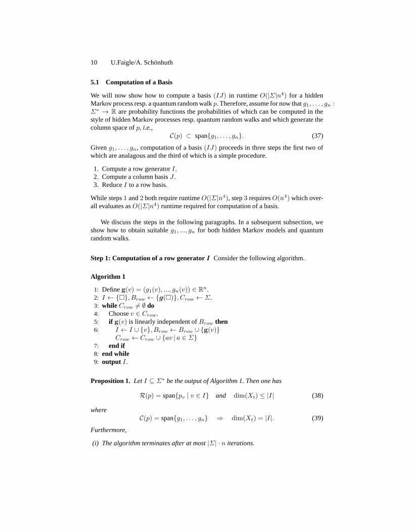
5.1 Computation of a Basis

We will now show how to compute a basis(IJ) in runtimeO(|Σ|n4) for a hiddenMarkov process resp. a quantum random walkp. Therefore, assume for now thatg1, . . . , gn :Σ∗ → R are probability functions the probabilities of which can becomputed in thestyle of hidden Markov processes resp. quantum random walksand which generate thecolumn space ofp, i.e.,

C(p) ⊂ span{g1, . . . , gn}. (37)

Giveng1, . . . , gn, computation of a basis(IJ) proceeds in three steps the first two ofwhich are analagous and the third of which is a simple procedure.

1. Compute a row generatorI.2. Compute a column basisJ .3. ReduceI to a row basis.

While steps1 and2 both require runtimeO(|Σ|n4), step3 requiresO(n4) which over-all evaluates asO(|Σ|n4) runtime required for computation of a basis.

We discuss the steps in the following paragraphs. In a subsequent subsection, weshow how to obtain suitableg1, ..., gn for both hidden Markov models and quantumrandom walks.

Step 1: Computation of a row generatorI Consider the following algorithm.

Algorithm 1

1: Defineg(v) = (g1(v), ..., gn(v)) ∈ Rn.2: I ← {�}, Brow ← {g(�)}, Crow ← Σ.3: while Crow 6= ∅ do4: Choosev ∈ Crow.5: if g(v) is linearly independent ofBrow then6: I ← I ∪ {v}, Brow ← Brow ∪ {g(v)}

Crow ← Crow ∪ {av | a ∈ Σ}7: end if8: end while9: output I.

Proposition 1. LetI ⊆ Σ∗ be the output of Algorithm 1. Then one has

R(p) = span{pv | v ∈ I} and dim(Xt) ≤ |I| (38)

whereC(p) = span{g1, . . . , gn} ⇒ dim(Xt) = |I|. (39)

Furthermore,

(i) The algorithm terminates after at most|Σ| · n iterations.

Efficient Equivalence Tests 11

(ii) Each iteration requiresO(n3) arithmetic operations where at mostn iterationsneed additionalO(|Σ|n3) operations.

Proof. Ad (i): Because then-dimensional vectors inBrow are independent|Brow| ≤n and|I| ≤ n follow immediately. Since at mostΣ words are added toCrow upon dis-covery of ann-dimensional vector which is linearly independent of thosein Brow, wehave|Crow| ≤ |Σ| · n and hence at most|Σ| · n iterations.

Ad (ii): In each iteration, we perform a test for linear independency of at mostnvectors of dimensionn which requires at mostO(n3) arithmetic operations [10]. In theat mostn cases whereg(v) is linearly independent ofBrow, we proceed by computing

(g1(av), ..., gn(av)) and (←−g1(av), ...,←−gn(av)) (40)

for all a ∈ Σ where(←−g1(v), ...,←−gn(v)) are available from an iteration before (note that

gi(�) = 1,←−gi(�) = (1, ..., 1) in the first iteration). Due to lemma 1, (35), this requiresO(|Σ| · n3) operations.

To prove (38), letv0 ∈ Σ∗ be arbitrary and suppose

g(v0) /∈ span{g(v) | v ∈ I}. (41)

We will derive a contradiction. Indeed, the algorithm can only missv0 if v0 had neverbeen collected intoCrow in step 6. This happens only in case that there is aw0 ∈ Σ∗

suchv0 = v1w0 holds for somev1 ∈ Σ∗ andg(w0) had been found to be linearlydependent of[g(v)]v∈I .

However, this is a contradiction to Lemma 2 below, which states that in such a casepv0 ∈ span{pv | v ∈ I} holds.

To see (39) letdim(Xt) < |I|. Since|I| = |Brow| we obtain that

dim C(p) = dim(Xt) < |Brow| ≤ dim span{g1, . . . , gn} (42)

henceC(p) ( span{g1, . . . , gn}. ⋄

Lemma 2. Let g1, . . . , gn : Σ∗ → R be such such thatC(p) ⊆ span{g1, . . . , gn} andlet v0, v1, ..., vm ∈ Σ∗ be such that

(g1(v0), ..., gn(v0)) ∈ span{(g1(vj), ..., gn(vj)) | j = 1, ...,m} ⊆ Rn. (43)

Then one has for everyw ∈ Σ∗:

pwv0 ∈ span{pwvj | j = 1, ...,m} ⊆ Rn. (44)

The analogous statement holds for the row spaceR(p).

12 U.Faigle/A. Schonhuth

Proof. By our hypothesis, there are scalarsβ1, ..., βm ∈ R such that

(g1(v0), ..., gn(v0)) =

m∑

j=1

βj(g1(vj), ..., gn(vj)). (45)

Letu ∈ Σ∗ be arbitrary. Again by our hypothesis, there are scalarsαi, i = 1, ..., n ∈ R

such that

pu =

n∑

i=1

αigi. (46)

We now compute

pu(v0)(46)=

n∑

i=1

αigi(v0)

(45)=

n∑

i=1

αi

m∑

j=1

βjgi(vj) =

m∑

j=1

βj

n∑

i=1

αigi(vj)

(46)=

m∑

j=1

βjgu(vj) =

m∑

j=1

βjp(uvj) =

m∑

j=1

βjpvj (u).

Since theβj had been determined independently ofu, we thus conclude

pv0 =

m∑

j=1

βjpvj . (47)

Let σw be the linear operator onR(c) with the property

σwpv = pvw. (48)

Application ofσw to (47) then shows

pv0w = σw(pv0) =

m∑

j=1

βjσw(pvj ) =

m∑

j=1

βjpvjw, (49)

which implies (44). ⋄

Step 2: Computation of a column basisJ Having obtained the row generatorI ⊆ Σ∗

in the step before, that isdim(Xt) ≤ |I| and

R(p) = span{pv | v ∈ I}, (50)

we can now use these functionspv as an input for an algorithm which is analogous tothat for computing the row generatorI.

Efficient Equivalence Tests 13

Algorithm 2

1: Defineq(w) := (pv(w) = p(wv), v ∈ I) ∈ R|I|.2: J ← {�}, Bcol ← {qw(�)}, Ccol ← Σ3: while Crow 6= ∅ do4: Choosew ∈ Ccol.5: if q(w) is linearly independent ofBcol then6: Acol ← Acol ∪ {w}, Bcol ← Bcol ∪ {q(w)}

Ccol ← Ccol ∪ {wa | a ∈ Σ}7: end if8: end while9: output J

While this routine is, in essence, analogous to algorithm 1,there is one differenceto be observed: HereCcol gets augmented by joiningwa whereasCrow, in algorithm1, was augmented by joiningav. This asymmetry is due to that one obtains an equiv-alently asymmetric statement in lemma 2 when rephrasing it forR(p) instead ofC(p).As a consequence, application of (34) instead of (35) in lemma 1 is needed.

We obtain thatPIJ = [p(wv)]v∈I,w∈J (51)

is a generator for(Xt). SinceR(p) = span{pv | v ∈ I}, by applying (39), we see that

|J | = dim(Xt). (52)

HenceJ is a genuine column basis. We recall that this was not necessarily the case forI which can happen to occur in the caseC(p) ( span{g1, ..., gn}.

All p(wav), v ∈ I, w ∈ J, a ∈ Σ can be obtained in runtimeO(|Σ| · n4) throughapplication of (36) in lemma 1 making use of the−→p (w),←−p (v) which were computedwhen executing the algorithms 1, 2.

We conclude: all necessary quantities can be obtained throughO(|Σ|·n4) arithmeticoperations.

Step 3: MakingI a basis This step is simple: one removesv fromI wherep(wv), w ∈J is linearly dependent inPIJ . This reduces the possibly too large setI to a row basisand finally yields a basis(IJ) for (Xt). This requires at mostn linear independencetests ofn-dimensional vectors henceO(n4) runtime [10].

5.2 Generating sets

Let us call a set{g1, . . . , gn} of functionsgi as in the previous section a set ofgener-ators for the column spaceC(p) of the hidden Markov process resp. quantum randomwalk (Xt).

We can get sets of generators as follows for which probabilitiesgi(v) can be com-puted in the style of hidden Markov processes resp. quantum random walks as follows.

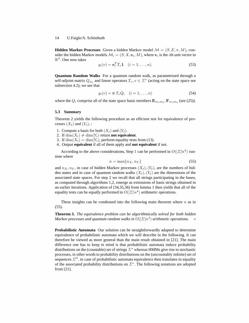
14 U.Faigle/A. Schonhuth

Hidden Markov ProcessesGiven a hidden Markov modelM = (S,E, π,M), con-sider the hidden Markov modelsMi = (S,X, ei,M), whereei is theith unit vector inRS . One now takes

gi(v) = eTi Tv1 (i = 1, . . . , n). (53)

Quantum Random Walks For a quantum random walk, as parametrized through aself-adjoint matrixQψ0

and linear operatorsTv, v ∈ Σ∗ (acting on the state space seesubsection 4.2), we see that

gi(v) = tr TvQi (i = 1, . . . , n) (54)

where theQi comprise all of the state space basis membersEm1m2,Fm1m2

(see (25)).

5.3 Summary

Theorem 2 yields the following procedure as an efficient testfor equivalence of pro-cesses(Xt) and(Yt), :

1. Compute a basis for both(Xt) and(Yt).2. If dim(Xt) 6= dim(Yt) returnnot equivalent.3. If dim(Xt) = dim(Yt), perform equality tests from (13).4. Outputequivalent if all of them apply andnot equivalent if not.

According to the above considerations, Step1 can be performed inO(|Σ|n4) run-time where

n = max{nX , nY } (55)

andnX , nY , in case of hidden Markov processes(Xt), (Yt), are the numbers of hid-den states and in case of quantum random walks(Xt), (Yt) are the dimensions of theassociated state spaces. For step2 we recall that all strings participating in the bases,as computed through algorithms 1,2, emerge as extensions ofbasis strings obtained inan earlier iterations. Application of (34,35,36) from lemma 1 then yields that all of theequality tests can be equally performed inO(|Σ|n4) arithmetic operations.

These insights can be condensed into the following main theorem wheren as in(55).

Theorem 3. The equivalence problem can be algorithmically solved for both hiddenMarkov processes and quantum random walks inO(|Σ|n4) arithmetic operations. ⋄

Probabilistic Automata Our solution can be straightforwardly adapted to determineequivalence of probabilistic automata which we will describe in the following. It cantherefore be viewed as more general than the main result obtained in [21]. The maindifference one has to keep in mind is that probabilistic automata induce probabilitydistributions on the (countable) set of stringsΣ∗ whereas HMMs give rise to stochasticprocesses, in other words to probability distributions on the (uncountably infinite) set ofsequencesΣN. in case of probabilistic automata equivalence then translates to equalityof the associated probability distributions onΣ∗. The following notations are adoptedfrom [21].

Efficient Equivalence Tests 15

Corollary 1. LetA1 = (S1, Σ,M1, π1, F1),A2 = (S2, Σ,M2, π2, F2) be two prob-abilistic automata whereN1 = |S1|, N2 = |S2|. Then equivalence ofA1,A2 can bedetermined inO((|Σ|+ 1)N4) whereN = max(N1, N2).

Proof. By adding a special symbol$ to Σ which is emitted from the final stateswith probability1 the automataA1,A2 can be transformed into probabilistic automatawith no final probabilitiesA1, A2. Let pA1

, pA2be the resulting stochastic processes.

According to [5], lemmata3 − 5, proposition8, probabilistic automata with no finalprobabilities can be can be viewed as HMMsM1,M2 which translates to that for eachv ∈ Σ∗

pA1(v) = pM1

(v) and pA2(v) = pM2

(v). (56)

Note that the transformation fromA1,2 toM1,2 requires only constant time. Applyingtheorem 1 toM1,M2 yields the result. ⋄

In short, corollary scales down the runtimeO((N1+N2)4) (the size of the alphabet

|Σ| is not discussed in [21]) toO((max(N1, N2))4).

Ergodicity Tests In [20], a generic algorithmic strategy for testing ergodicity of hid-den Markov processes was described, where overall efficiency hinged on computationof a basis of the tested hidden Markov processes. The algorithms described above re-solve this issue. Hence ergodicity of hidden Markov processes can be efficiently tested.Similarly to the equivalence tests, the ergodicity test of [20] solely requires that theprocess in question is finitary. Therefore this efficient ergodicity test equally applies forquantum random walks.

5.4 Conclusive Remarks

We have presented a polynomial-time algorithm by which to efficiently test both hid-den Markov processes and quantum random walks for equivalence. Previous solutionsavailable for hidden Markov processes had runtime exponential in the number of hid-den states. To test equivalence for quantum random walks, that is random walk modelsto be emulated on quantum computers, is relevant for the samereasons that apply forhidden Markov processes. An algorithm for testing equivalence for quantum randomwalks had not been available before. Note that the algorithmpresented here is easy toimplement and, in particular for hidden Markov processes, only requires invocation ofwell-known standard routines. Future directions are to explore how to efficiently testfor similarity of hidden Markov processes and quantum random walks where similarityis measured in terms ofapproximate equivalence. Such tests have traditionally been ofgreat practical interest.

References

1. D. Aharonov, A. Ambainis, J. Kempe, U. Vazirani: “Quantumwalks on graphs”,Proc. of33rd ACM STOC, New York, pp. 50–59, 2001.

2. A. Ambainis: “Quantum search algorithms”,SIGACT News, vol. 35(2), pp. 22-35, 2004.

16 U.Faigle/A. Schonhuth

3. D. Blackwell and L. Koopmans: “On the identifiability problem for functions of finiteMarkov chains”,Annals of Mathematical Statistics, vol. 28, pp. 1011–1015, 1957.

4. M.A. Nielsen and I.L. Chuang: “Quantum Computation and Quantum Information”,Cam-bridge University Press, Cambridge, UK, 2000.

5. P. Dupont, F. Denis and Y. Esposito: “Links between probabilistic automata and hiddenMarkov models: probability distributions, learning models and induction algorithms”,Pat-tern Recognition, vol. 38, pp. 1349–1371, 2005.

6. Durbin, Eddy, Krogh: “Biological Sequence Analysis” Cambridge University Press, 1998(XXX: check)

7. Y. Ephraim and N. Merhav: “Hidden Markov Processes”,IEEE Transactions on Informa-tion Theory, vol. 48, 1518-1569, 2002.

8. U. Faigle and A. Schoenhuth: ”Asymptotic mean stationarity of sources with finite evolu-tion dimension”,IEEE Transactions on Information Theory, vol. 53, 2342-2348, 2007.

9. U. Faigle and A. Schoenhuth: ”Discrete Quantum Markov Chains”, Preprint 2010, submit-ted.

10. D. K. Faddeev and V. N. Faddeeva: “Computational Methodsof Linear Algebra”,Freeman,San Francisco, 1963.

11. E.J. Gilbert: “On the identifiability problem for functions of finite Markov chains”,Annalsof Mathematical Statistics, vol. 30, pp. 688–697, 1959.

12. A. Heller: “On stochastic processes derived from Markovchains”,Annals of MathematicalStatistics, vol. 36, pp. 1286–1291, 1965.

13. H. Ito, S.-I. Amari and K. Kobayashi: “Identifiability ofhidden Markov information sourcesand their minimum degrees of freedom”,IEEE Trans. Inf. Theory, vol. 38(2), pp. 324–333,1992.

14. H. Jager: “Observable operator models for discrete stochastic time series”,Neural Compu-tation, vol. 12(6), pp. 1371–1398, 2000.

15. J. Kempe: “Quantum random walks hit exponentially faster”, Probability Theory and Re-lated Fields, vol. 133(2), pp. 215–235, 2005.

16. F.L. Marquezino, R. Portugal, G. Abal and R. Donangelo: “Mixing times in quantum walkson the hypercube”,Phys. Rev. A, 77, 042312, 2008.

17. Y. Ephraim, N. Merhav, ”Hidden Markov processes”,IEEE Trans. on Information Theory,vol. 48(6), pp. 1518-1569, 2002.

18. R. Pintelon, J. Schoukens, “System Identification”,IEEE Press, Piscataway, NJ, 2001.19. L.R. Rabiner: “A tutorial on hidden Markov models and selected applications in speech

recognition”,Proceedings of the IEEE, vol. 77, pp. 257-286, 1989.20. A. Schonhuth, H. Jaeger: “Characterization of ergodichidden Markov sources”,IEEE

Transactions on Information Theory, vol. 55, pp. 2107-2118, 2009.21. W.-G. Tzeng: “A polynomial-time algorithm for the equivalence of probabilistic automata”,

SIAM Journal of Computing, vol. 21, pp. 216-227, 1992.