Support vector method for robust ARMA system identification

IEEE TRANSACTIONS ON SIGNAL PROCESSING, VOL. 52, NO. 1, JANUARY 2004 155

Support Vector Method for RobustARMA System Identification

José Luis Rojo-Álvarez, Member, IEEE, Manel Martínez-Ramón, Member, IEEE,Mario de Prado-Cumplido, Student Member, IEEE, Antonio Artés-Rodríguez, Senior Member, IEEE, and

Aníbal R. Figueiras-Vidal, Senior Member, IEEE

Abstract—This paper presents a new approach to auto-regres-sive and moving average (ARMA) modeling based on the supportvector method (SVM) for identification applications. A statisticalanalysis of the characteristics of the proposed method is carriedout. An analytical relationship between residuals and SVM-ARMAcoefficients allows the linking of the fundamentals of SVM withseveral classical system identification methods. Additionally, theeffect of outliers can be cancelled. Application examples show theperformance of SVM-ARMA algorithm when it is compared withother system identification methods.

Index Terms—ARMA modeling, cross-correlation, supportvector method, system identification, time series.

I. INTRODUCTION

AFREQUENT approach to digital signal processing isto propose a model composed by two discrete-time

processes (DTP), which are the input and the output to a linear,time-invariant system (LTIS). An LTIS is usually approximatedby means of a rational transfer function that can be an all-zeroor moving average (MA), an all-pole or auto-regressive (AR),or a general zero-pole (ARMA) system. ARMA modeling isuseful in problems such as system identification, time-seriesanalysis, spectral analysis, and deconvolution. A number ofapplications for ARMA modeling can be enumerated. Forexample, in digital communications, channel identificationprovides a way of reducing intersymbol interference; in addi-tion, channels of multiuser detection schemes can be viewed asmultiple-input multiple-output systems, and the MA structureis used to compensate the effect of multipath signal propagation[1]. In radar signal processing, adaptiveness is better achievedby means of ARMA implementations, getting advantage withrespect to the Fourier transform in the robust determination ofDoppler spectrum [2], [3]. Biomedical signals can be analyzedto build models for diagnosis purposes; spectral analysis ofthe heart-rate variability and its relationship to blood pressurevariability are useful in arrhythmia risk stratification of patientswith previous myocardial infarction [4]; cardiovascular modelsof the aortic vein state can be estimated from blood pressureand flow measurements [5]; and spectral analyses of electroen-cephalographic potentials enable a deeper knowledge of thebrain [6].

Manuscript received December 10, 2002; revised April 10, 2003. This workwas supported in part by CICYT under Grants TIC 1999-0216 and TIC 2000-0380-C03-03. The associate editor coordinating the review of this paper andapproving it for publication was Prof. Ioan Tabus.

The authors are with the Department of Signal Theory and Communications,University Carlos III de Madrid, 28911 Leganés, Madrid, Spain.

Digital Object Identifier 10.1109/TSP.2003.820084

Classical ARMA estimation methods present some limita-tions.

• Analysis of DTP with atypical samples (outliers) is neithereasy nor immediate, and it is usually achieved by heuristicor even visual inspection methods [12]. So, the use of ro-bust cost functions to avoid the effect of outliers oftenarises numerical optimization disadvantages.

• In general terms, ARMA methods require a previous de-termination of model complexity or number of parametersin the model, and they are quite sensitive to wrong orderchoice [9].

• Finally, error surfaces are not convex in many cases. Evenworse, sample-based approximations to convex theoreticalsurfaces can exhibit local minima.

In this paper, we introduce a new approach to ARMA mod-eling that is based on the support vector method (SVM). TheSVM was first proposed to obtain maximum margin separatinghyperplanes in classification problems [13], but this techniquehas become a general learning theory [14], [15]. A comprehen-sive description of this method for classification and regressionproblems can be found in [16] and [17], respectively. Althoughsome previous work has been done with SVM regression andtime series analysis [7], [8], the algorithm that we present isformulated for system identification: a framework where robust-ness is specially needed. Robustness is just a main feature thatSVM controls, as it will be shown in this paper. Besides, we de-velop a statistical analysis of the characteristics of our method.In addition, we pay special attention to the cost function usedin this SVM approach, which is a scarcely discussed aspect inSVM regression literature, although it has a key relevance insignal processing environments.

The approach to ARMA system identification drawn fromSVM minimizes a regularized cost functional of the residuals.Potential advantages of SVM are the following.

• It provides a unique solution.• It is a strongly regularized method, which is appropriate

for ill-posed problems.• It extracts the maximum information from the available

samples, although the statistical distribution is unknown.Consequently, SVM can diminish some of the limitations of

classical ARMA system identification methods, as we will seebelow in more detail.

The structure of the paper is as follows. In Section II, we in-troduce SVM-ARMA system identification equations, and wepropose a robust cost function that leads to the corresponding

1053-587X/04$20.00 © 2004 IEEE

156 IEEE TRANSACTIONS ON SIGNAL PROCESSING, VOL. 52, NO. 1, JANUARY 2004

SVM-ARMA algorithm. Then, the relationship between resid-uals and SVM-ARMA coefficients is analyzed in Section III,yielding a useful statistical interpretation of SVM-ARMAterms. This allows the establishment of a comparison with clas-sical system identification methods. Simulation and applicationexamples are included in Section IV. Finally, in Section V,conclusions are drawn.

II. SVM-ARMA FORMULATION

Let us consider two DTPs and , which are theinput and the output, respectively, of a rational LTIS. The cor-responding difference equation is

(1)

where and are the AR and MA coefficients ofthe system, respectively, and is a DTP standing for theeffect of measurement errors.

Let us also consider a set of consecutive samples ofand a set of consecutive samples of observed at thesame time instants. The difference equation can be used to set arelationship among observations, estimated parameters, and er-rors. In this case, error terms , or residuals, comprehendboth measurement and model approximation errors. In orderto consider initial conditions, (1) is required only for time-lags

, where . Assuming thatand (also known as model order) can be properly chosen

beforehand, ARMA coefficients are usually estimatedfrom minimizing a cost functional, depending on the residuals.

In general, SVM algorithms for linear classification and re-gression problems minimize a cost function for the residuals(CFR) that is called Vapnik’s (or -insensitive) loss function,which is given by

ifif

(2)

and this CFR is regularized with the norm of the model pa-rameters [13], [18]. Whereas , SVM allows to obtainsparse solutions where the estimated classification or regressionfunction depends only on a reduced number of the set of ob-served samples; these samples are called support vectors. Theextension of SVM to nonlinear classifiers and regressors can beeasily achieved by using Mercer’s kernels.

An additional free parameter must be previously fixed tocontrol the tradeoff between the cost of the residuals and theregularization term. This tradeoff is chosen according to somea priori knowledge of the problem or by using cross-valida-tion techniques. The resulting functional is usually optimizedvia quadratic programming (QP) [19].

We propose to use Vapnik’s CFR plus an regularization,including both the AR and the MA model coefficients, to createwhat we call SVM-ARMA modeling. This corresponds to theunconstrained minimization of

(3)

An equivalent formulation of the above process [13] is to min-imize

(4)

where , and are slack variables or losses constrained to

(5)

(6)

(7)

for , where denotes both and . Theprimal-dual or Lagrange functional for this problem is obtainedby introducing a nonnegative coefficient (Lagrange multiplier)for each constraint [19], yielding

(8)

where the multipliers are constrained to and, and (7) also stands. Equation (8) has to be minimized with

respect to primal variables , , and and maximized withrespect to Lagrange multipliers (also called dual variables)and .

From

(9)

several consequences are drawn. First, dual variables are shownto be constrained between an upper and a lower bound

(10)

ROJO-ÁLVAREZ et al.: SUPPORT VECTOR METHOD FOR ROBUST ARMA SYSTEM IDENTIFICATION 157

for . Second, we can observe that

(11)

(12)

show the analytical relationship among the model coefficients,the dual coefficients, and the observations. Third, these condi-tions can be introduced into Lagrange functional (8) to removethe primal variables. After that, another term grouping can bedone in by writing down

(13)

(14)

These equations denote the time-local th- and th-ordersample estimators of the values of the autocorrelation functionsof the input and the output DTP and , re-spectively.

By introducing (13) and (14) into (8), the problem can beexpressed in terms of the residual constraints and the data, andit is stated in vector-matrix form as the maximization of

(15)

under constrains (10), and where and

.This is a QP problem, and if we write

(16)

(17)

(18)

then the aim is to maximize with respect tounder some linear constraints. It is clear that matrix is notinvertible and the solution is unfeasible. Like in SVM regression[17], this problem can be ad hoc regularized by adding a smallvalue diagonal matrix, i.e., by replacing the square matrix by

. Matrix can be easily shown to be definitepositive, and the resulting constrained QP problem has a singleminimum, thus avoiding the local minima problems in the LSsolution of the normal ARMA system identification equations[9].

Note that the above-mentioned numerical regularization isapparently different from the -norm regularization of theprimal functional in (4); in fact, this numerical regularizationis not always reported in SVM regression literature, and it isfrequently treated as a simple numerical trick. However, thenumerical regularization in the dual problem can be seen as anadditional term in the dual functional, given by the norm of

Fig. 1. Robust CFR for the SVM-ARMA algorithm. There are three different(possible) regions, allowing us to deal with different kinds of noise.

the Lagrange coefficients. This means that the QP problem weare really solving is the maximization of

(19)

constrained to (10).Several robust cost functions have been used in SVM regres-

sion, such as Vapnik’s loss function [13], Huber’s robust cost[7], or the ridge regression approach [20]. Here, we propose amore general cost function that has the above-mentioned ones asparticular cases. Proposed robust CFR is depicted in Fig. 1, andit can be expressed as the following piecewise-defined function:

(20)

where . The three different intervals of serveto deal with different kinds of noise. Insensitive zone isadequate for low-frequency variations such as wander or base-line deviations. The quadratic cost zone takes into account theobservation noise, the norm in this zone being appropriatefor Gaussian processes. The linear cost zone limits the effect ofeither outliers or jitter noise on the model parameter estimation.

Thus, the proposed robust SVM-ARMA algorithm is statedas the minimization of this robust CFR plus the regularizationterm:

(21)

constrained to (5)–(7), where is the set of samples for which, and is the set of samples for which .

Appendix A shows that the dual problem corresponding to (21)is equivalent to (19) in the sense that both reach their optimumfor the same values of Lagrange coefficients. This fact permitsa twofold interpretation.

• When considering Vapnik’s loss function as the cost on theresiduals, the regularized cost function for SVM-ARMAwe are really working with is not (4), but rather (21), dueto the effect of the numerical regularization.


• Far from being a disadvantage, considering the quadraticcost zone will allow to work with a more general costfunction than Vapnik’s cost and for some kinds of DTP, itcan be useful to set an appropriate value for free parameter

.Note that three free parameters ( and ) are to be tuned.

These parameters can be a priori fixed according to the statis-tical model of DTPs. Selecting leads to Huber’s robustcost function [21]. In addition, represents Vapnik’s func-tion, showing that it becomes nondifferentiable at inthe absence of numerical regularization. In a number of applica-tions, some knowledge of the statistical properties of DTPs canbe available. So, it will be desirable relating (20) to other costcriteria by establishing a general class of robust cost functions.When noise is Gaussian, the quadratic cost will be the most ap-propriate; however, in this case, insensitivity should be removed

, and sparsity will not be achieved. For sub-Gaussiannoise, a better performance could be obtained with a cubic orhigher degree cost zone. If super-Gaussian (for instance, impul-sive or heavy-tails) noise is present, it will be convenient to seta low value for product but with so that we will nothave an ill-posed problem.

III. STATISTICAL INTERPRETATION

The consideration of the cost function in (20) allows us totrace an analytical relationship between residuals and Lagrangemultipliers in the SVM-ARMA algorithm (21). Let bethe Lagrange coefficients in the solution. Then, residuals andcoefficients are related in the form

.

(22)

This analytical relationship is proved in Appendix B fromKarush-Khun-Tucker (KKT) conditions when the solution ofthe QP problem is reached.

Analytical relationship (22) between Lagrange multipliersand residuals in SVM-ARMA algorithm (21) allows us tocompare the latter with classical algorithms. Although a reallyvast number of methods for system identification have beensuggested, Ljung points out in [9] that there are two maingeneral procedures. On the one hand, prediction-error methods(PEMs) are based on the minimization of a function of theresidual power for a given model. PEMs contain well-knownprocedures such as the least-squares (LS) method, and they areclosely related to Bayesian maximum a posteriori estimation[10]. On the other hand, correlation methods (CMs) seek forthe minimization of the cross-correlation between a functionof the residuals and a transformation of the data, possiblydepending on the parameter vector; this approach includes theinstrumental-variable 4 method (from now, Iv4), as well asseveral procedures for rational transfer function modeling [11].Here, we present a brief comparison of SVM-ARMA with bothkinds of methods.

Comparison with PEM: If , , then Lagrangemultipliers are just proportional to the residuals. To highlight

Fig. 2. Geometrical interpretation of error bias. LS solution v producesan unbiased averaged error d that is orthogonal to the space spanned by thedata, whereas the SVM solution v can be seen as a regularized but biasedsolution with increased approximation averaged error e.

the bias-variance dilemma in SVM-ARMA versus LS systemidentification, a geometrical interpretation based on the orthog-onality principle will be carried out. For the sake of simplicity,let us consider the projection of a vector onto the sub-space generated by data , as depicted in Fig. 2. Accordingto LS criterion, the projection is denoted as ,whereas SVM projection is . SVM pro-jection is obtained as the result of minimizing

(23)

constrained to . From

(24)

the following relationships can be established for the coeffi-cients of both solutions:

(25)

from which

(26)

(27)

Accordingly, SVM-ARMA coefficients given by (11) and(12) can be seen as the minimum norm projection of thesolution onto the subspace that is generated by the inputsignal, the output signal, and their delayed versions. The modelcoefficients are calculated as the dot product between thenonlinearized error and the subspace base vectors.

If the observation noise is Gaussian, and the observed datahave actually been generated by an ARMA model, i.e.,

, then is an unbiased estimator of the modelcoefficients [9], and for the th coefficient , we have

(28)

where denotes statistical expectation of a random variable.However, is a biased estimator since

(29)


and the bias is due to the regularization term. Additionally, thevariance of the LS estimator is

(30)

whereas the variance of the SVM estimator is

(31)

In this case, biased SVM-ARMA will provide better estima-tors only if its variance is below LS variance, i.e.,

(32)

As a consequence, in the presence of Gaussian noise andfor an underlying ARMA model, the LS parameter estimatoris the optimum solution in the sense of unbiased error. Here,SVM-ARMA algorithm will be able to provide a biased (yetreduced variance) estimator whenever LS estimator variance isgreater than the true ARMA coefficient; this can be the case insituations having a low number of observation samples, true co-efficients of low amplitude, or low signal-to-noise ratio (SNR).

Comparison with CM: As previously mentioned, CM arebased on the assumption that a good model produces residuals,regardless of past data. They also seek the minimization ofthe cross-correlation between a function of the residuals and atransformation of the data. The open issue in this setting is howto find both the residual function and the data transformation.

In order to relate SVM-ARMA algorithm with CM, we startfrom the case , , and (quadratic lossonly), which again leads to Lagrange multipliers that are equalto the residuals. In this case, prediction coefficients and

are sample estimates (except for a scaling factor) of thecross-correlation between the residuals and the data. Using (22)in (11) and (12), and since

(33)

(34)

with , the coefficients can be seen as

(35)

(36)

This emphasizes the fact that the SVM-ARMA solution leadsto low correlation (in the given lags) between the residuals andthe data.

If or (or both), then is a nonlineartransformation of the residuals given by (22). In this case, themodel coefficients are estimated from the cross-correlation ofthe transformed residuals and the data

(37)

(38)

As long as we impose the minimum norm of the coefficients,the sample correlation between this nonlinear function of theresiduals and the data is reduced. Taking into account (11) and

(12), one can see the relationship to the general CM equation[9]. Note that there is no data transformation, but instead, theresidual nonlinear function is based on the statistical knowledgeof the errors, which is incorporated into the free parameters ofCFR.

Finally, the comparison with CM suggests the possibility ofa new algorithm by forcing the residuals to be uncorrelatedwith the data for more lags than and . This could be easilyachieved by forcing coefficients to be small or even zerofor , .

IV. APPLICATION EXAMPLES

In the applications that we will present here for the systemidentification SVM-ARMA algorithm, attention will be paidto some of its main features. First, a simulation example al-lows us to appreciate the performance when outliers are present.Second, a classical example (Feedback’s Process Trainer [9]) isused to compare SVM-ARMA with several system identifica-tion methods. Finally, a real-world example is reported (the re-lationship between simultaneous heart rate and diastolic bloodpressure), where erroneous measurement values often appear.Two performance measurements are used: the error of the ap-proximation to the true impulse response of the LTIS when it isknown (example A) and the prediction error on a validation setwhen real data are analyzed (examples B and C).

A. Insensitivity to Outliers

The test system to be identified is

(39)

This system is chosen because its impulse response hassamples with amplitudes of different orders of magnitude.Input DTP is a white, Gaussian noise sequence of unit variance,which will be denoted . The correspondingoutput DTP is corrupted by an additive, small variance randomprocess , modeling the measurement errors.This leads to an observed process . Thenumber of observed samples is chosen to be low, be-cause SVM algorithms are expected to work well in low-sizeddata sets, mainly due to their strong regularization.

Impulsive noise is generated as a sparse sequence, for which30% of the samples, randomly placed, are of high-amplitude,having the form [where denotes the uniformdistribution in the given interval]. The remaining are zero sam-ples. This noise sequence is denoted by . The observationsconsist of DTP input and the observed output plus impul-sive noise, i.e., . Values of go from 18 to0 dB.

As insensitivity to outliers is expected to be reduced by thelinear zone of the empirical cost, is used, and true or-ders for both numerator and denominator are introduced intothe model. An extremely low value of leads to a higher em-phasis on minimizing the losses so that overfitting can occur.Then, we select a moderately high . The appropriatechoice of can be addressed by considering that according to(35) and (36), the solution is a function of Lagrange multipliers


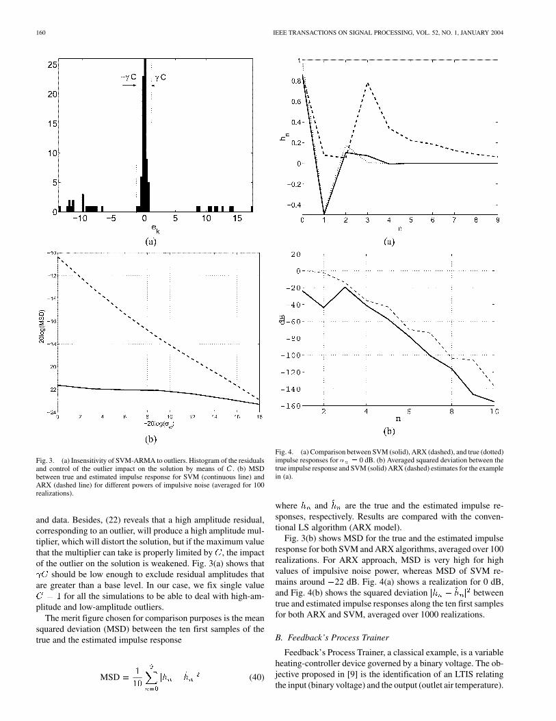
Fig. 3. (a) Insensitivity of SVM-ARMA to outliers. Histogram of the residualsand control of the outlier impact on the solution by means of C . (b) MSDbetween true and estimated impulse response for SVM (continuous line) andARX (dashed line) for different powers of impulsive noise (averaged for 100realizations).

and data. Besides, (22) reveals that a high amplitude residual,corresponding to an outlier, will produce a high amplitude mul-tiplier, which will distort the solution, but if the maximum valuethat the multiplier can take is properly limited by , the impactof the outlier on the solution is weakened. Fig. 3(a) shows that

should be low enough to exclude residual amplitudes thatare greater than a base level. In our case, we fix single value

for all the simulations to be able to deal with high-am-plitude and low-amplitude outliers.

The merit figure chosen for comparison purposes is the meansquared deviation (MSD) between the ten first samples of thetrue and the estimated impulse response

MSD (40)

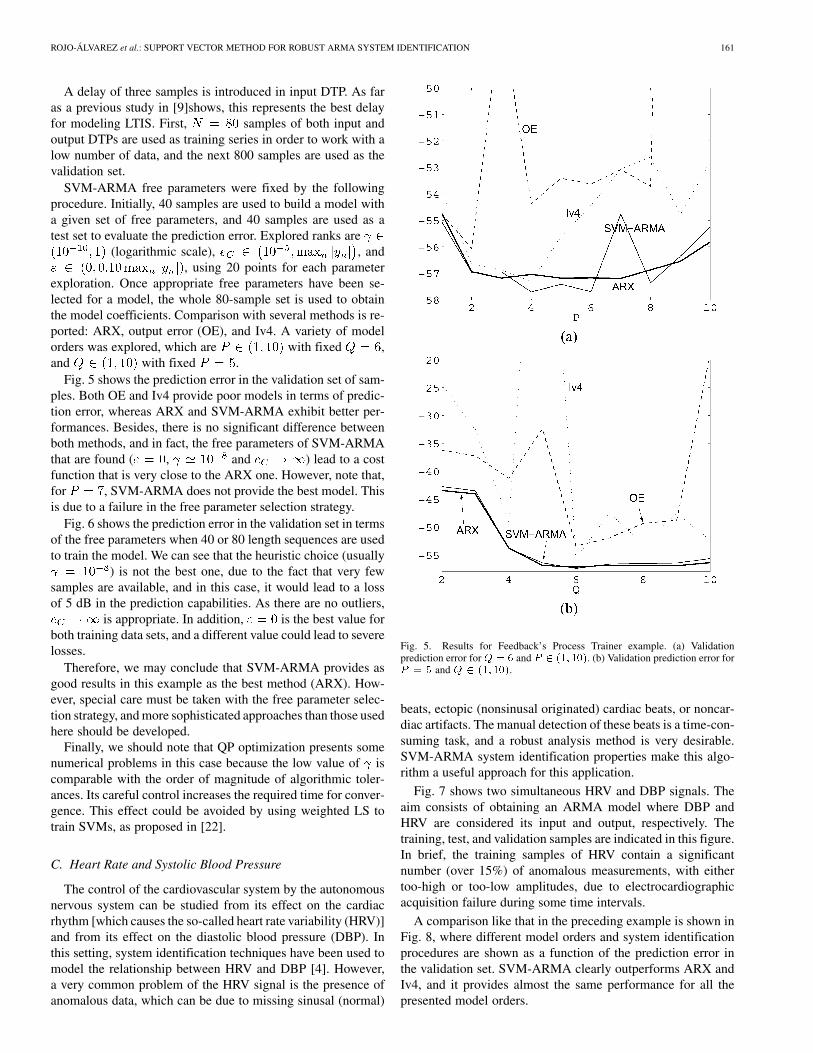
Fig. 4. (a) Comparison between SVM (solid), ARX (dashed), and true (dotted)impulse responses for � = 0 dB. (b) Averaged squared deviation between thetrue impulse response and SVM (solid) ARX (dashed) estimates for the examplein (a).

where and are the true and the estimated impulse re-sponses, respectively. Results are compared with the conven-tional LS algorithm (ARX model).

Fig. 3(b) shows MSD for the true and the estimated impulseresponse for both SVM and ARX algorithms, averaged over 100realizations. For ARX approach, MSD is very high for highvalues of impulsive noise power, whereas MSD of SVM re-mains around 22 dB. Fig. 4(a) shows a realization for 0 dB,and Fig. 4(b) shows the squared deviation betweentrue and estimated impulse responses along the ten first samplesfor both ARX and SVM, averaged over 1000 realizations.

B. Feedback’s Process Trainer

Feedback’s Process Trainer, a classical example, is a variableheating-controller device governed by a binary voltage. The ob-jective proposed in [9] is the identification of an LTIS relatingthe input (binary voltage) and the output (outlet air temperature).


A delay of three samples is introduced in input DTP. As faras a previous study in [9]shows, this represents the best delayfor modeling LTIS. First, samples of both input andoutput DTPs are used as training series in order to work with alow number of data, and the next 800 samples are used as thevalidation set.

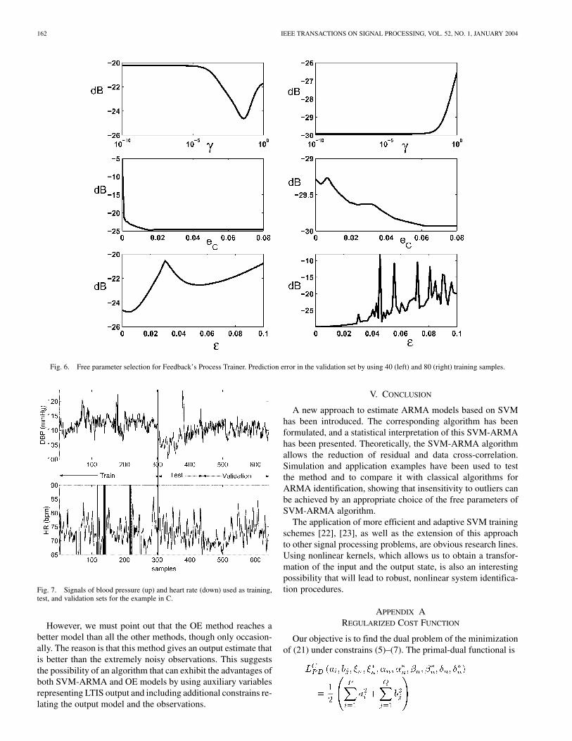
SVM-ARMA free parameters were fixed by the followingprocedure. Initially, 40 samples are used to build a model witha given set of free parameters, and 40 samples are used as atest set to evaluate the prediction error. Explored ranks are

(logarithmic scale), , and, using 20 points for each parameter

exploration. Once appropriate free parameters have been se-lected for a model, the whole 80-sample set is used to obtainthe model coefficients. Comparison with several methods is re-ported: ARX, output error (OE), and Iv4. A variety of modelorders was explored, which are with fixed ,and with fixed .

Fig. 5 shows the prediction error in the validation set of sam-ples. Both OE and Iv4 provide poor models in terms of predic-tion error, whereas ARX and SVM-ARMA exhibit better per-formances. Besides, there is no significant difference betweenboth methods, and in fact, the free parameters of SVM-ARMAthat are found ( , and ) lead to a costfunction that is very close to the ARX one. However, note that,for , SVM-ARMA does not provide the best model. Thisis due to a failure in the free parameter selection strategy.

Fig. 6 shows the prediction error in the validation set in termsof the free parameters when 40 or 80 length sequences are usedto train the model. We can see that the heuristic choice (usually

) is not the best one, due to the fact that very fewsamples are available, and in this case, it would lead to a lossof 5 dB in the prediction capabilities. As there are no outliers,

is appropriate. In addition, is the best value forboth training data sets, and a different value could lead to severelosses.

Therefore, we may conclude that SVM-ARMA provides asgood results in this example as the best method (ARX). How-ever, special care must be taken with the free parameter selec-tion strategy, and more sophisticated approaches than those usedhere should be developed.

Finally, we should note that QP optimization presents somenumerical problems in this case because the low value of iscomparable with the order of magnitude of algorithmic toler-ances. Its careful control increases the required time for conver-gence. This effect could be avoided by using weighted LS totrain SVMs, as proposed in [22].

C. Heart Rate and Systolic Blood Pressure

The control of the cardiovascular system by the autonomousnervous system can be studied from its effect on the cardiacrhythm [which causes the so-called heart rate variability (HRV)]and from its effect on the diastolic blood pressure (DBP). Inthis setting, system identification techniques have been used tomodel the relationship between HRV and DBP [4]. However,a very common problem of the HRV signal is the presence ofanomalous data, which can be due to missing sinusal (normal)

Fig. 5. Results for Feedback’s Process Trainer example. (a) Validationprediction error for Q = 6 and P 2 (1; 10). (b) Validation prediction error forP = 5 and Q 2 (1; 10).

beats, ectopic (nonsinusal originated) cardiac beats, or noncar-diac artifacts. The manual detection of these beats is a time-con-suming task, and a robust analysis method is very desirable.SVM-ARMA system identification properties make this algo-rithm a useful approach for this application.

Fig. 7 shows two simultaneous HRV and DBP signals. Theaim consists of obtaining an ARMA model where DBP andHRV are considered its input and output, respectively. Thetraining, test, and validation samples are indicated in this figure.In brief, the training samples of HRV contain a significantnumber (over 15%) of anomalous measurements, with eithertoo-high or too-low amplitudes, due to electrocardiographicacquisition failure during some time intervals.

A comparison like that in the preceding example is shown inFig. 8, where different model orders and system identificationprocedures are shown as a function of the prediction error inthe validation set. SVM-ARMA clearly outperforms ARX andIv4, and it provides almost the same performance for all thepresented model orders.


Fig. 6. Free parameter selection for Feedback’s Process Trainer. Prediction error in the validation set by using 40 (left) and 80 (right) training samples.

Fig. 7. Signals of blood pressure (up) and heart rate (down) used as training,test, and validation sets for the example in C.

However, we must point out that the OE method reaches abetter model than all the other methods, though only occasion-ally. The reason is that this method gives an output estimate thatis better than the extremely noisy observations. This suggeststhe possibility of an algorithm that can exhibit the advantages ofboth SVM-ARMA and OE models by using auxiliary variablesrepresenting LTIS output and including additional constrains re-lating the output model and the observations.

V. CONCLUSION

A new approach to estimate ARMA models based on SVMhas been introduced. The corresponding algorithm has beenformulated, and a statistical interpretation of this SVM-ARMAhas been presented. Theoretically, the SVM-ARMA algorithmallows the reduction of residual and data cross-correlation.Simulation and application examples have been used to testthe method and to compare it with classical algorithms forARMA identification, showing that insensitivity to outliers canbe achieved by an appropriate choice of the free parameters ofSVM-ARMA algorithm.

The application of more efficient and adaptive SVM trainingschemes [22], [23], as well as the extension of this approachto other signal processing problems, are obvious research lines.Using nonlinear kernels, which allows us to obtain a transfor-mation of the input and the output state, is also an interestingpossibility that will lead to robust, nonlinear system identifica-tion procedures.

APPENDIX AREGULARIZED COST FUNCTION

Our objective is to find the dual problem of the minimizationof (21) under constrains (5)–(7). The primal-dual functional is


Fig. 8. Results for the heart rate and blood pressure example. (a) Validationprediction error for Q = 5 and P 2 (1; 20). (b) Validation prediction error forP = 5 and Q 2 (1;10).

(41)

constrained to

(42)

By zeroing the derivative of with respect to the primalvariables, we obtain the expression for the prediction coeffi-cients as a function of Lagrange multipliers. However, a dif-ference appears when calculating the derivatives with respect to

with , for which

(43)

It is clear that and, necessarily, , so that

(44)

and denoting by the constant value

(45)

it is easy to see that

(46)

where is given by (19). This reveals that both functionsreach the minimum at the same values of Lagrange multipliers.

APPENDIX BRESIDUALS AND LAGRANGE COEFFICIENTS

The analytical relationship presented in (22) must be sepa-rately shown for three different cases, according to the differentKKT conditions for each one.

Case 1) For , we find that and .In the solution, the values reached by the primal andthe dual functional are equal. Therefore, taking intoaccount (11) and (12), the following equation holds:

(47)

Derivatives of the constraints corresponding tovanish at the solution. Thus, using the chain rule, weobtain, by zeroing the derivative of (47)

(48)

and hence

(49)

The derivation is similar for ,just considering that, in this case, , and

.


Case 2) When , it is straightforward to see thatcorresponding vanish.

Case 3) When , the Lagrange multiplier directioncannot be greater than , and hence, . Sim-ilar considerations can be made for .

REFERENCES

[1] N. D. Sidiropoulos and G. Z. Dimic, “Blind multiuser detection inW-CDMA systems with large delay spread,” in IEEE Signal ProcessingLett., vol. 8, Mar. 2001, pp. 87–89.

[2] S. Haykin and A. Steinhart, Adaptive Radar Detection and Estima-tion. New York: Wiley, 1992.

[3] S. de Waele and P. M. T. Broersen, “Modeling radar data with time seriesmodels,” in Proc. EUSIPCO, Tampere, Finland, Sept. 2000, Ref. 116.

[4] Task force of the European Society of Cardiology and the North Amer-ican Society of Pacing and Electrophysiology, “Heart rate variability.Standards of measurement, physiological interpretation and clinicaluse,” Eur. Heart J., vol. 17, pp. 354–381, Mar. 1996.

[5] C. Vlachopoulos and M. O’Rourke, “Genesis of normal and abnormalarterial pulse,” Current Prob. Cardiol., vol. 25, pp. 297–368, 2000.

[6] J. D. Bronzino, The Biomedical Engineering Hadbook. Boca Raton,FL: CRC/IEEE, 1995.

[7] K. R. Müller et al., “Predicting time series with support vector ma-chines,” in Advances in Kernel Methods—Support Vector Learning,B. Scholkopf et al., Eds. Cambridge, MA: MIT Press, 1999, pp.243–254.

[8] S. Mukherjee, E. Osuna, and F. Girosi, “Nonlinear prediction of chaotictime series using support vector machines,” in Proc. IEEE NNSP,Amelia Island, FL, Sept. 1997, pp. 511–519.

[9] L. Ljung, System Identification. Theory for the User, 2nded. Englewood Cliffs, NJ: Prentice-Hall, 1999.

[10] T. C. Hsia, Identification: Least Squares Methods. Lexington, MA:Lexington Books, 1977.

[11] T. Söderström and P. Stoica, System Identification. Englewood Cliffs,NJ: Prentice-Hall, 1987.

[12] J. Li, K. Miyashita, T. Kato, and S. Miyazaki, “GPS time series modelingby autoregressive moving average method: Application to the crustal de-formation in central Japan,” Earth Planets Space, vol. 52, pp. 155–162,Feb. 2000.

[13] V. Vapnik, The Nature of Statistical Learning Theory. New York:Springer-Verlag, 1995.

[14] B. Schölkopf and K. Sung, “Comparing support vector machines withGaussian kernels to radial basis function classifiers,” IEEE Trans. SignalProcessing, vol. 45, pp. 2758–2765, Nov. 1997.

[15] M. Pontil and A. Verri, “Support vector machines for 3D object recogni-tion,” IEEE Trans. Pattern Anal. Machine Intell., vol. 20, pp. 637–646,June 1998.

[16] C. J. C. Burges, “A tutorial on support vector machines for pattern recog-nition,” Data Mining Knowl. Discovery, vol. 2, pp. 1–32, Jan. 1998.

[17] A. J. Smola and B. Schölkopf, “A tutorial on support vector regression,”ESPRIT, Neural and Computational Learning Theory NeuroCOLT2NC2-TR-1998-030, 1998.

[18] A. N. Tikhonov and V. Y. Arsenin, Solution to Ill-Posed Prob-lems. Washington, DC: V.H. Winston, 1977.

[19] D. G. Luenberger, Linear and Nonlinear Programming. Reading, MA:Addison-Wesley, 1984.

[20] N. Cristianini and J. S. Taylor, An Introduction to Support Vector Ma-chines and Other Kernel-Based Learning Methods. Cambridge, U.K.:Cambridge Univ. Press, 2000.

[21] P. J. Huber, “Robust statistics: A review,” Ann. Stat., vol. 43, pp.1041–67, 1972.

[22] A. Navia-Vázquez, F. Pérez-Cruz, A. Artés-Rodríguez, and A. R.Figueiras-Vidal, “Weighted least squares training of support vectorclassifiers leading to compact and adaptive schemes,” IEEE Trans.Neural Networks, vol. 12, pp. 1047–1059, Sept. 2001.

[23] F. Pérez-Cruz, A. Navia-Vázquez, P. L. Alarcón-Diana, and A. Artés-Rodríguez, “An IRWLS procedure for SVR,” in Proc. EUSIPCO, Tam-pere, Finland, Sept. 2000, Ref. 156.

José Luis Rojo-Álvarez (M’01) received thetelecom engineer degree from University of Vigo,Vigo, Spain, in 1996 and the Ph.D. degree intelecommunication from the Polytechnical Univer-sity of Madrid, Madrid, Spain, in 2000.

He is an Assistant Professor with the Departmentof Signal Theory and Communications, UniversityCarlos III, Madrid. His main research interests in-clude statistical learning theory, digital signal pro-cessing, and complex system modeling, with appli-cations both to digital communications and to car-

diac signal processing. He has published work on cardiac arrhythmia and ar-rhythmia-genesis mechanisms, robust analysis, and echocardiographic imageand hemodynamic function evaluation.

Manel Martínez-Ramón (M’00) received thetelecom engineer degree from Politechnical Uni-versity of Catalunya, Barcelona, Spain, in 1994 andthe Ph.D. degree in telecommunication from theUniversity Carlos III, Madrid, Spain, in 1999.

He is a Visitant Professor with the Departmentof Signal Theory and Communications, UniversityCarlos III. His main research interests includestatistical learning theory, digital signal processing,and communications, with applications to digitalcommunications, areas of research on he has

published several works.

Mario de Prado-Cumplido (S’02) was born inMadrid, Spain, on December 1977. He receivedthe M.Sc. degree in telecommunication engineeringfrom the Universidad Politécnica de Madrid in 2000.He is currently pursuing the Ph.D. degree at Univer-sidad Carlos III, Madrid, where he is doing researchon machine learning algorithms, feature selection,and probability density estimation techniques andtheir application to biomedical problems, withparticular attention to cardiovascular pathologies.

Antonio Artés-Rodríguez (M’89–SM’01) was bornin Alhama de Almería, Spain, in 1963. He receivedthe Ingeniero de Telecomunicación and Doctor In-geniero de Telecomunicación degrees, both from theUniversidad Politécnica de Madrid, Spain, in 1988and 1992, respectively.

He is now a Professor with the Departamento deTeoría de la Señal y Comunicaciones, UniversidadCarlos III, Madrid. His research interests include de-tection, estimation, and statistical learning methodsand their application to signal processing and com-

munication.

Aníbal R. Figueiras-Vidal (S’74–M’76–SM’84)received the Telecom. Engineer degree from Univer-sidad Politécnica de Madrid, Madrid, Spain, in 1973(ranked number 1; National Award to graduation)and the Doctor degree (Honors) from UniversidadPolitécnica de Barcelona, Barcelona, Spain, in 1976.

He is a Professor of signal theory and commu-nications with Universidad Carlos III, Madrid. Hisresearch interests are digital signal processing,digital communications, neural networks, andlearning theory. He has (co)authored more than 300

journal and conference papers in these areas.Dr. Figueiras received an “Honoris Causa” Doctorate degree in 1999 from

Universidad de Vigo, Vigo, Spain. He is currently General Secretary of theAcademy of Engineering of Spain.

Support vector method for robust ARMA system identification

Documents

Transcript of Support vector method for robust ARMA system identification