Bayesian Modeling of Autoregressive PartialLinear Models with Scale Mixture of Normal

Errors

Guillermo Ferreira,1 Luis M. Castro,2 Victor H. Lachos3 and Ronaldo Dias 4

April 24, 2012

Abstract

Normality and independence of error terms is a typical assumption for partial linear mod-els. However, such an assumption may be unrealistic on many fields such as economics,finance and biostatistics. In this paper, we develop a Bayesian analysis for partial linearmodel with first-order autoregressive errors belonging to the class of scale mixtures of normal(SMN) distributions. The proposed model provides a useful generalization of the symmet-rical linear regression models with independent error, since the error distribution cover bothcorrelated and thick-tailed distributions, and has a convenient hierarchical representation al-lowing to us an easily implementation of a Markov chain Monte Carlo (MCMC) scheme. Inorder to examine the robustness of this model against outlying and influential observations,we present a Bayesian case deletion influence diagnostics based on the Kullback-Leibler(K-L) divergence. The proposed methodology is applied to the Cuprum Company monthlyreturns.

Keywords: Autoregressive Time Series Model, Gibbs Sampler, Influential Observations,Partial Linear Models, Scale Mixtures of Normal Distributions..

1 Departamento de Estadıstica, Facultad de Ciencias Fısicas y Matematicas, Universidad de Concepcion,Concepcion, Chile. E-mail: gferreir@udec.cl

2 Departamento de Estadıstica, Facultad de Ciencias Fısicas y Matematicas, Universidad de Concepcion,Concepcion, Chile. E-mail: luiscastroc@udec.cl

3 DepartamentodeEstatıstica,IMECC,Universidade Estadual de Campinas, Campinas, Sao Paulo, Brazil. E-mail: hlachos@ime.unicamp.br

4DepartamentodeEstatıstica,IMECC,Universidade Estadual de Campinas, Campinas, Sao Paulo, Brazil.E-mail: dias@ime.unicamp.br

Corresponding author: Guillermo Ferreira, Departamento de Estadıstica, Facultad de Ciencias Fısicas yMatematicas, Universidad de Concepcion, Concepcion, Chile. E-mail: gferreir@udec.cl

1. Introduction

It is a standard assumption for regression models that all random errors are mutuallyindependent. However, in some situations, this assumption is not necessarily appropriate.Situations in which data are collected sequentially over the time may give rise to substantialserial correlation in the errors [40]. Consequently, autoregressive models could be a practicalsolution for modeling this type of data. Specifically, we consider the process Yt following theregression model with first-order autoregressive stationary errors given by

Yt = x>t β + g(t) + εt, t = 1, . . . , T (1)

where xt is a vector of explanatory variables, β are the regression parameters, g(·) is anunknown smooth function of the auxiliary covariate t and εt is the sequence of autoregressiveerrors. This model is well known as a partial linear model and it is usually considered as asemi-parametric model since it contain both a parametric linear term and a non-parametriccomponent. In fact, in this type of model it is assumed that the mean response is linearlydependent on some covariates, whereas its relation to other variables is characterized by non-parametric functions.

Partial linear models have become an important tool in modeling economic and biomet-ric data and many authors have been proposed the estimation of β and g in various contextsincluding kernel smoothing, smoothing splines and penalized splines from the classical andBayesian points of view. For example, [48] proposed a semi-parametric model for longitu-dinal data in order to model the evolution of CD4 cell numbers in HIV seroconverters. [16]provided improvements in semi-parametric regression in time series studies of air pollutionin the context of GAM models. [23] considered robust generalized estimating equations forthe analysis of semi-parametric generalized partial linear models for longitudinal data.

Related to the Bayesian analysis of autoregressive errors, [8] developed a practical frame-work for the Bayesian analysis for normal and Student-t regression models under autocor-related errors. In this context, [30] considered applications of the Gibbs Sampler, showingthat the sampler applies nicely to various autoregressive processes. Besides, [42] have beendeveloped a practical and exact methods of analyzing ARMA(p, q) regression models in aBayesian framework by using the Gibbs sampling and Metropolis-Hastings algorithms.

More recently, and from the classical point of view, [33] have been study the influencediagnostics for linear models with first-order autoregressive elliptical errors, whereas [26]have analyzed a partial linear model with Student-t independent errors.

In this context, natural extensions for the model proposed by [26] can be obtained by as-suming that the distribution of the perturbations belongs to the scale mixture of normal (SMN)distributions family [see 1], from which the normal and Student-t models can be obtained asspecial cases. This class of distributions constitutes a class of thick-tailed distributions, someof which are the slash and the contaminated normal distributions.

To the best of our knowledge, there are no studies on Bayesian inference for the partiallinear models with autocorrelated errors belonging to the SMN family. Consequently, inthis paper we propose a Bayesian approach of the model (1) considering the distribution ofcorrelated errors εt belonging to the class of SMN distributions. In addition, we propose aBayesian influence diagnostic based on Kullback-Leibler (K-L) distance.

The outline of the paper is as follows. In Section 2 we give a brief introduction to theSMN class of distributions. In Section 3 we define the partial linear model with autoregressiveerrors. In Section 4 we propose the Bayesian approach for the partial linear model and wediscuss the use of prior information. In Section 5 we review influence measures based on K-Ldivergence. The main advantages of the proposed methodology are discussed via simulation

2

studies in Section 6. In Section 7, we analyze the monthly returns series of the CuprumCompany. Finally, Section 8 closes the paper with some conclusions.

2. Scale-mixtures of normal distributions familiy (SMN family)

A random variable Y belongs to the SMN family if it can be written as

Y = µ+ ω−1/2Z, (2)

where µ is a location parameter, Z ∼ N(0, σ2), ω is a positive random variable with cdfH(· | ν) and pdf h(· | ν); and ν is a scalar or vector parameter indexing the distribution ofω. Given ω, we have Y | ω ∼ N(µ, ω−1σ2). Thus, the pdf of Y is given by

fSMN(y | µ, σ2,ν) =

∫ ∞0

φ(y | µ, ω−1σ2)dH(ω | ν), (3)

where φ(· | µ, σ2) denotes the density of the univariate N(µ, σ2) distribution. The notationY ∼ SMN(µ, σ2,ν) will be used when Y has pdf as in (3). As was mentioned above, theSMN family constitutes a class of thick-tailed distributions including various sub-classes,some of which are the normal distribution when ω = 1, the Student-t distribution, de-noted by T(µ, σ2, ν), when ω ∼ Gamma(ν/2, ν/2), ν > 0; the slash distribution denoted bySL(µ, σ2, ν) when ω ∼ Beta(ν, 1), ν > 0 and the contaminated normal distribution, denotedby CN(µ, σ2, ν, γ) with ν, γ ∈ (0, 1), when ω is a discrete random variable taking one of twostates 1 or γ, with probability function given by h(ω | ν) = νI(ω = γ) + (1 − ν)I(ω = 1).We refer to [1] for details and additional properties related to this class of distributions.

3. Partial linear models with autoregressive SMN errors

3.1. The modelIn this section, we extend the classical partial linear model by introducing autocorrelated

errors defined as a discrete time autoregressive process. The discrete time representation ofthis model for the observed response at the time t is given by

Yt = x>t β + g(t) + εt, (4)εt = ρεt−1 + ηt, t = 1, . . . , T,

where Yt denotes the response variable, xt is a k × 1 vector of non-stochastic explanatoryvariable values, β is a k × 1 fixed parameter vector, t is a scalar, g is a smooth function,εt is the first-order autoregressive error with disturbance ηt belonging to the SMN family ofdistributions i.e. ηt ∼ SMN(0, σ2

η,ν) and ρ is the autoregressive coefficient (| ρ |< 1).The autoregressive model proposed in (4) has may applications in economical, agricul-

tural, biological and biomedical problems. For example, in predicting future stock prices, theeffect of an intervention might persist for some time, besides business and economics; seefor example [20] and [39]. It is important to stress that normal regression models with timeseries errors have received considerable attention in recent years. For example, [47], [31] and[6] give a complete review about time series regression models.

3

3.2. The likelihood functionAn alternative way of writing model (4) is given by

Yt = x>t β + g(t) + ρ[Yt−1 − x>t−1β − g(t− 1)

]+ ηt, t = 1, . . . , T. (5)

It is important to stress that for (5), we will use the conditional representation because it isvery useful since it allows us to write the likelihood function in a closed form. In fact, by theMarkov property, the conditional density of Yt with respect to Y1, Y2, . . . , Yt−1 is the same asthe conditional density of Yt with respect to Yt−1. Since ηt ∼ SMN(0, σ2

η,ν), the likelihoodfunction for an observed sample y = (y1, . . . , yT )> can be expressed by

L(θ | y) = fSMN(y1 | µ, σ2η,ν)

T∏t=2

[fSMN(yt | yt−1, µ, σ

2η,ν)

]

∝T∏t=2

[fSMN(yt | yt−1, µ, σ

2η,ν)

](6)

where µ(t) = x>t β+g(t)+ρ[yt−1 − x>t−1β − g(t− 1)

]and θ = (β, ρ, σ2

η,ν) [for numerousadvantages of conditional likelihoods see 4].

Our proposal considers the Bayesian paradigm for a number of reasons, primarily mo-tivated by the computational simplicity achieved. From the classical point of view, one ofthe difficulties for the partial linear model estimation is the maximization of the the penal-ized log-likelihood function, since under non-gaussian models the estimating equations aretypically nonlinear and require the implementation of iterative procedures. For example,[21] proposed a Newton-Raphson algorithm to solve the penalized estimating equations inthe semi-parametric case. The EM-type algorithm has also been applied in semi-parametricmodeling [see 41], but its routine for complicated autoregressive models is computationallycumbersome, and hence a single run of this algorithm is often more time consuming than theBayesian updating.

On the other hand, the high-dimensional integrals involved in the SMN likelihood func-tion further complicates ML-type estimation. Nevertheless, recent developments in Markovchain Monte Carlo (MCMC) methods facilitate easy and straightforward implementation ofthe Bayesian paradigm through conventional softwares like WinBUGS or OpenBUGS.

4. Bayesian implementation

The unknown non-parametric function g(t) is modeled by using penalized spline (P-spline) smooth function. Recently, penalized spline fitting has become very popular smooth-ing technique because of the link between smoothing functions and linear mixed modelswhich makes the procedure so attractive. Based on a suggestion by [13], this connectionis made by using pth-degree spline basis for representing g(t) by α0 + α1t + . . . + αpt

p +∑Ks=1 bs(t − κs)

p+, where κ1 ≤ κ2 . . . ≤ κK are fixed knots, and these knots are typically

placed at quantiles of the distribution of unique values of the covariate t. With respect to thedimension K we follow [38] recommendation that the actual choice of K and the location ofknots have little influence on the resulting penalized fit as long as K is large. The value ofK is chosen between 5 and 35 to ensure enough flexibility [see 37]. The random coefficientof the P-spline function b is assumed to be normally distributed with zero mean and varianceσ2b . A Bayesian penalized spline has the advantage of allowing for simultaneous estimation

of smooth functions and smoothing parameters.

4

4.1. Model specificationIn order to represent the model given by the equation (4) in the semi-parametric context,

we proceed as in [38] by considering a mixed model representation of a penalized spline, i.e.,

Yt = w>t Λ + z>t bt + εt, (7)

where wt = (x>t , t>)> and Λ = (β>,α>)>,withα = (α0, · · · , αp)> and t = (1, t, . . . , tp)>,

include the fixed and polynomial component of the model, z>t bt =∑K

s=1 bs(t−κs)p+ includes

the spline basis functions and εt represents the autoregressive error. As in Section (3), we canwrite the model (7) as

Yt = m(t) + ρ [Yt−1 − m(t− 1)] + ηt, t = 1, . . . , T, (8)

where m(t) = w>t Λ + z>t bt. Therefore, the autoregressive partial linear model can be easilyrepresented as follows:

Yt | Λ, ρ, σ2η, Yt−1,bt, ωt ∼ N(µ(t), ω−1

t σ2η), for 2 ≤ t ≤ T, (9)

bt | σ2b ∼ NK(0, σ2

bIK), for 1 ≤ t ≤ T, (10)ωt | ν ∼ H(ωt;ν), for 1 ≤ t ≤ T , (11)

where µ(t) = m(t) + ρ [Yt−1 − m(t− 1)]. It is important to stress that for t = 1, theconditional distribution for Y1 given Λ, ρ, σ2

η,b1, ω1 is N(m(1), [ωt(1− ρ2)]−1σ2

η

).

4.2. Prior distributionsIn order to complete the Bayesian specification, we need to consider prior distributions for

all unknown model parameters θ = (β>,α>, ρ, σ2η,ν)>. We propose the prior distributions

for the parametric and non-parametric components as follows.

• Parametric component: A popular choice to ensure posterior propriety in a linear modelis to consider proper (but diffuse) conditionally conjugate priors [25, 50]. Besides weused a reparameterization for ρ given by 2ρ? − 1, with ρ? ∈ (0, 1). This reparam-eterization allows us to specify a beta distribution as a prior for ρ?. In this context,[29] proposed a beta distribution instead of a uniform distribution, because the betadistribution represents extremely well a stationary autoregressive process, while theuniform distribution prior represents better the case of a random walk generating pro-cess. Specifically, we have that

β ∼ Nk(β0,Ω0), (12)ρ? ∼ Beta(aρ? , bρ?), (13)σ2η ∼ IGamma(q0/2, q1/2), (14)

where Beta(·, ·) is the beta distribution and IGamma(c, d) is the inverse gamma distri-bution with mean d/(c− 1), c > 1, d > 0. For the specific SMN models, the prior forν was chosen accordingly as follows.

(i) Student-t model: Here ν ∼ TExp(λ/2; (2,∞)), i.e., the degrees of freedom pa-rameter ν has a truncated exponential prior distribution on the interval (2,∞).This truncation point was chosen to assure finite variance.

(ii) Slash model: A Gamma(a, b) distribution with small positive values of a and b(b a) is adopted as a prior distribution for ν.

5

(iii) Contaminated normal model: A Beta(ν0, ν1) distribution is used as a prior for ν,and an independent Beta(γ0, γ1) is adopted as prior for γ.

• Non-parametric component: Likewise, for the non-parametric function g(.) we haveunknown parameters for fixed effects components and random effects components. Forthe fixed components, α = (α0, . . . , αp)

> we consider

α ∼ Np(0,Σ0). (15)

When the prior distributions for unknown parameters have been assessed, the next step isto combine the likelihood function (6) with the prior information in order to make Bayesianinference. This procedure is implemented by using a MCMC scheme.

4.3. Implementation of MCMC algorithmThe MCMC scheme was implemented using WinBUGS through the bugs() function im-

plemented in the package R2WinBUGS [see 45] called from R software [see 35]. The programcodes are available from the author upon request. When the MCMC implementation is ap-plied to the simulated data (see Section 6), convergence of the MCMC samples is assessedusing standard tools within WinBUGS software (trace plots, ACF plots, as well as Gelman-Rubin convergence diagnostic). After an initial 50000 burn-in iterations, 2500 samples withthinning 20 are obtained to make inference. After fitting these models, we also use a Bayesianmodel selection technique to choose the best model that fits the data in Section 7.

Let be the vectors ω = (ω1, . . . , ωT )> and b = (b>1 , . . . ,b>T )>.Thus, conditionally on

yt−1 and ω, all conditional posterior distributions are as in a standard normal model and havethe same form for any element of the SMN family. In fact, by considering the conditionalrepresentation (9-11) of the SMN partial linear model (7) and the prior specifications in (12)-(15), a Metropolis-within-Gibbs sampling algorithm could be implemented as follows:

Λ | θ,y,b,ω ∼ Nk+3(AΛµΛ, AΛ),

σ2η | θ,y,b,ω ∼ IGamma

(q0 + T

2,q1 + s

2

),

ν | θ,y,b,ω ∝ π(ν)T∏t=1

h(ωt | ν),

ρ? | θ,y,b,ω ∝ π(ρ?)(1− ρ2)1/2

× exp

−σ2−1η

2

((1− ρ2)ω1 [y1 − m(1)]2 +

T∑t=2

[yt − µ(t)]2)

,

bt | θ,y,b(−t),ω ∼ NK (Ctµb, Ct) ,

ωt | θ,y,b,ω(−t) ∼ ω(T−1)/2t h(ωt | ν) exp

−ωt

(yt − µ(t)√

2ση

)2,

for t = 2, · · · , T , where

µΛ = ∆−1Λ Λ0 + σ2−1

η (1− ρ2)ω1e1w1 + σ2−1η

T∑t=2

ωt [et − ρet−1] (wt − ρwt−1),

AΛ =

[∆−1

Λ + σ2−1η

(ω1w1w

>1 (1− ρ2) +

T∑t=2

ωt(wt − ρwt−1)(w>t − ρw>t−1)

)]−1

,

µb = z>t[(yt −w>t Λ)− ρ(yt−1 −w>t−1Λ) + z>t−1bt−1

],

6

and et = yt − z>t bt, Ct =(σ2−1b IK + σ2−1

η ωtztz>t

)−1, ρ = 2ρ? − 1, Λ0 = (β>0 , 0, 0, 0)>,

∆Λ = (Ω0,Σ0) and s = (1− ρ2)ω1(e1 −w>1 Λ)2 +∑T

t=2 ωt [yt − µ(t)]2 . For t = 1, we havethat,

b1 | θ,y1,ω1 ∼ NK

(C1z

>1 (y1 −w>1 Λ), C1

),

ω1 | θ,y1,b ∼ ω1/21 h(ω1 | ν) exp

−ω1(1− ρ2)

(e1 −w>1 Λ√

2ση

)2

where C1 =(σ2−1b IK + σ2−1

η (1− ρ2)ω1z1z>1

)−1.

As was mentioned above, the full conditionals for ωt, ν and ρ? require Metropolis-Hastings steps. Specifically, for the case of ωt and ν, the Metropolis-Hastings step willdepend on the form of the pdf h(ωt | ν). The full conditional distributions for a specific SMNdistribution are given in the Appendix.

5. Bayesian model selection and influence diagnostics

5.1. Model comparison criteriaOne of the most used methodologies to compare several competing models for a given

data set is derived from the conditional predictive ordinate CPO statistic [see 19, 7]. Lety = (y1, y2, · · · , yn) the full data and y(i) = (y1, y2, · · · , yi−1, yi+1, · · · , yn) denote the datawith the ith observation deleted. For the ith observation, the CPO is defined as

CPOi = f(yi | y(i)) =

∫θ∈Θ

f(yi | θ, y(i))π(θ | y(i))dθ

The CPO is a cross-validated predictive approach i.e. predictive distributions conditioned onthe observed data with a single data point deleted. In this paper, we propose to modify theCPO in order to obtain what we call the autoregressive CPO, which is computed for each newobservation using only the data from previous time periods.

Let y` = (y1, y2, · · · , y`) be the data vector at time point ` and yT = y1, y2 · · · , yT bethe complete data set. In our autoregressive context, the CPO at each time period is given by

CPOt = f(yt | yt−1) =

∫θ∈Θ

f(yt | θ,yt−1)π(θ | yt−1)dθ, t = 2, · · · , T.

where f(yt | θ,yt−1) =∫∞

0φ(yt | µ(t), ω−1σ2

η)dH(ω | ν), for t = 2, · · · , T and for t = 1

we have f(y1 | θ) =∫∞

0φ(y1 | m(1), ω−1σ2

η/ρ2)dH(ω | ν).

Since for the proposed model a closed form of the CPOt is not available, a Monte Carloestimate of the CPOt is obtained by using a single MCMC sample from the posterior distri-bution π(θ | y). Let θ1, . . . ,θQ be a sample of size Q of π(θ | y) after the burn-in. A MonteCarlo approximation of the CPOt is given by the following expression (for its proof see theAppendix):

CPOt =

(1

Q

Q∑q=1

f(yt−1 | θq)f(yT | θq)

)−1(1

Q

Q∑q=1

f(yt | θq)f(yT | θq)

).

In addition, a summary statistic of the CPOt’s is the log pseudo marginal likelihood (LPML),

defined by LPML=T∑t=1

log(CPOt). Models with greater LMPL values will indicate a bet-

ter fit. Other Bayesian measure of goodness-of-fit and complexity for model selection is

7

the Deviance Information Criterion (DIC) proposed by [44]. This criterion is based on

the posterior mean of the deviance. It can be approximated by D =Q∑q=1

D(θq)/Q, where

D(θ) = −2T∑t=2

log[f(yt | yt−1,θ)

]. It is important to stress that, for t = 1 we used

f(y1 | θ) instead of f(yt | yt−1,θ). The DIC criterion can be estimated using MCMCoutput by DIC = D + ρD = 2D − D, where ρD is the effective number of parameters,which is defined as ED(θ) −D(Eθ), where D(Eθ) is the deviance evaluated at theposterior mean. Finally, D(Eθ) can be estimated as

D = D

(1

Q

Q∑q=1

βq,1

Q

Q∑q=1

σ2ηq,

1

Q

Q∑q=1

αq,1

Q

Q∑q=1

νq,1

Q

Q∑q=1

ρq

).

Given the comparison of two alternative models, the model that better fits a data set is themodel with the smallest value of the DIC. Note that it is important to integrate out all latentvariables in the deviance calculation as this yields a more appropriate penalty term ρD; [see27]. It is important to stress that for all these criteria, the evaluation of the likelihood functionL(θ | y) is a key aspect. However, for our autoregressive SMN partial linear model, thatfunction can be easily computed from the result given in Subsection 3.2.

Finally, the Expected Information Criteria (EAIC) and the Expected Bayesian Informa-tion Criteria (EBIC) can be estimated by mean of EAIC = D + 2](ϑ) and EBIC =D + ](ϑ) log(T ), where ](ϑ) is the number of model parameters [see 5].

5.2. Bayesian case influence diagnosticsSince regression models are sensitive to the underlying model assumptions, generally

performing a sensitivity analysis is strongly advisable. [10] uses this idea to motivate his as-sessment of influence analysis. He suggests that more confidence can be put in a model whichis relatively stable under small modifications. The best known perturbation schemes are basedon case-deletion [11] in which the effects are studied of completely removing cases from theanalysis. This reasoning will form the basis for our Bayesian global influence methodologyand by so doing it will be possible to determine which subjects might be influential for theanalysis in SMN autoregressive partial linear models.

In this paper, we propose to modify the K(P, P(−t)) between P and P(−t), where P de-notes the posterior distribution of θ for full data, and P(−t) denotes the posterior distributionof θ without the tth case.

The K(·, ·) utilized is computed for each new observation using only the data from previ-ous time periods. Specifically,

K(Pyt , Pyt−1) =

∫π(θ | yt) log

[π(θ | yt)π(θ | yt−1)

]dθ. (16)

K(Pyt , Pyt−1) thus measures the effect of t-th case from the vector of all the observations upto time t. For the proposed model in (4) it can be shown that (16) can be expressed as follows

K(Pyt , Pyt−1) = f(yt+1, . . . , yT | yt)[Eθ|y

log [f(yt | yt−1,θ)]

f(yt | θ)

f(yT | θ)

− log (CPO)Eθ|y

f(yt | θ)

f(yT | θ)

],

(17)

8

where Eθ|y(·) denotes the expectation with respect to the joint posterior π(θ | y). Thus (17)can be computed by sampling from the posterior distribution of θ via MCMC methods. Letθ1, . . . ,θQ be a sample of size Q of π(θ | y). Then, a Monte Carlo estimate of the K-Ldivergence, K(Pyt , Pyt−1), is given by

K(Pyt , Pyt−1) = f(yt+1, . . . , yT | yt)

[1

Q

Q∑q=1

log f(yt | yt−1,θq)f(yt | θq)f(yT | θq)

− log(CPOt)

1

Q

Q∑q=1

f(yt | θq)f(yT | θq)

].

(18)

It is important to stress that we derived an approximation for f(yt+1, . . . , yT | yt) based on aMonte Carlo integration procedure (see Appendix).

6. Simulation studies

6.1. Frequentist properties of Bayesian estimatesThe goal of this simulation study is to show the good behavior of the Bayesian estimates,

based on the frequentist mean squared error (MSE) and the frequentist mean (Mean), and themeasurement used for model comparison e.g. LPML, DIC, EAIC and EBIC. We performedthe simulation scheme with the following model

yt = 2xt1 + 4xt2 + g(t) + εt, (t = 1, 2, . . . , 200), (19)

where g(t) = −1−10(t2+t3)−5 cos (t+ t2 + t3) and εt = 0.30εt−1+ηt with ηt ∼ T (0, 1, 4).The covariates xt1 and xt2 were simulated from a uniform random sample i.e. xt1 ∼ U(0, 1)and xt2 ∼ U(2, 3). We generated 200 data sets. Once the data are simulated, we fitteda partial linear model, assuming that η′ts have a normal, Student-t, slash and contaminatednormal distributions.

The following independent priors are considered to perform the Bayesian approach:

(a) parametric component, βk ∼ N(0, 1.0−6), for k = 1, 2, ρ? ∼ Beta(20, 1.5), (σ2

η) ∼ Gamma(0.001, 0.001);

(b) non-parametric component, b ∼ N15(0, σ2bI15), σ2

b ∼ IGamma(0.001, 0.001) andαk ∼ N1(0, 106), for k = 1, 2, 3. In addition, we consider ν ∼ TExp(0.1; ((2,∞)))for the Student-t model; ν ∼ Gamma(0.1, 0.01) for the slash model; and ν ∼ U(0, 1)and γ ∼ Beta(2, 2) for the contaminated normal model.

For each generated data set we simulate three chains of size 50000 for each parameter,discarding the first 25000 and considering a spacing of size 10 in order to avoid correlationproblems.

We compute the MSE and the ”Relative Bias” (RelBias) as follows:

RelBias(θ) =1

200

200∑i=1

(θi/θ − 1

), and

MSE(θ) =1

200

200∑i=1

(θi− θ

)2

,

9

Table 1: Monte Carlo results based on 200 simulated samples.

Model β1 β2 ρ σ2 ν

Normal MC Mean 1.974 4.031 0.332 1.425MC sd 0.317 0.346 0.071 0.114

RelBias 0.022 0.048 0.329 0.425MSE 6.6e-04 9.5e-04 6.7e-03 1.8e-01

Student-t MC Mean 2.003 4.046 0.313 1.049 6.377MC sd 0.273 0.212 0.062 0.094 3.246

RelBias 0.002 0.012 0.223 0.049MSE 1.6e-05 2.2e-06 4.0e-04 2.4e-05

Slash MC Mean 1.984 3.998 0.311 0.887 4.634MC sd 0.309 0.285 0.065 0.111 6.900

RelBias 0.078 0.015 0.243 0.113MSE 2.5e-04 2.4e-04 3.6e-03 1.3e-02

Cont. Normal MC Mean 1.969 4.021 0.315 0.977 0.303MC sd 0.277 0.302 0.064 0.139 0.150

RelBias 0.046 0.025 0.262 0.123MSE 9.8e-04 4.4e-04 4.3e-03 5.2e-04

where θ = (β1, β2, ρ, σ2η) and θ

iis the posterior estimates of θ for the ith sample. From Table

(1), we observe that the Student-t model has the smallest RelBias and MSE for β1, β2 and ρ,indicating the efficiency of Bayesian estimation of the fixed-effects.

Table (2) presents the arithmetic mean of the measurement used for model comparison,i.e., LPML, DIC, EAIC and EBIC. We notice that all these measures favored the Student-t model for our simulated data showing the ability of these Bayesian selection methods todetect an obvious departure from normality.

Table 2: Comparison between normal and SMN models. MC indicate the MonteCarlo mean of the respective criteria.

Criteria

Model MC LPML MC DIC MC EAIC MC EBIC

Normal -358.9722 2111.9274 714.6778 727.8710Student-t -350.7098 2064.6609 700.4542 713.6475

Slash -352.6526 2100.4751 710.5232 718.5244Cont. normal -360.0623 2514.9974 713.4181 726.6114

6.2. Influence of outlying observationsThe goal of this simulation study is to investigate the consequences on parameter in-

ference when the normality assumption is inappropriate as well as to investigate whether

10

the model comparison measures, e.g., LPML, DIC, EAIC and EBIC determines the best-fitting model to the simulated data. In addition, we are interested in show the capacity of themethodology in order to detect atypical data and the sensitivity of the Bayesian estimatorsunder alternative distributions. For that reason we considered the case-weight perturbationscheme [for more detail for details see 49].

We assume the following autoregressive partial linear model given by

yt = 1.5xt1 + 3.5xt2 + g(t) + εt, (t = 1, 2, . . . , 300), (20)

where g(t) = −3−10t2−5 sin (t+ t2 + t3)−5 cos (t+ t2 + t3) and εt = 0.15εt−1 +ηt withηt ∼ N(0, 1). The covariates xt1 and xt2 were simulated from a uniform random sample,namely, xt1 ∼ U(0, 1) and xt2 ∼ U(2, 3). We selected cases 55 and 250 for perturbation. Tocreate influential observation in the data set, we choose one, or two of these selected casesand we perturbed the response variable as follows yt = yt + 4Sy, t = 55, 250, where Sy isthe standard deviations of the yt’s.

The MCMC computations were done in a similar way to those given in the last section.In order to monitor the convergence of the Markov chains we used some of the methodsrecommended by [12].

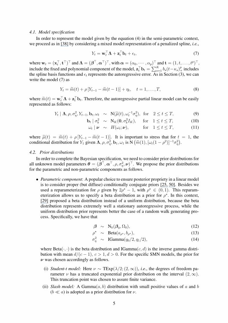
Table (3) shows that the posterior inferences are sensitive to the perturbation of the se-lected case(s). As expected, the estimates of β, σ2 and ρ under the SMN distributions areless affected than those under normal one. Table (4) reports the estimates of the EAIC, EBIC,LPML and DIC for each perturbed version of the original data set under different SMN mod-els. Once again we can see that the slash model presents a better fit.

Figure (1) shows the influence of the observations 55 and 250. We observed a high sen-sitivity of the Bayesian estimation in the presence of atypical data when the normal modelis considered. Figures (2)–(4) also show that the Bayesian estimates are more robust in thepresence of atypical data when the SMN distributions are used (a perturbed observation wasnot detected).

11

Table 3: Posterior mean and standard deviations of the parameters from fitting dif-ferent SMN models under normal data

NormalPerturbed β1 β2 ρ σ2

case Mean SD Mean SD Mean SD Mean SD

None 1.461 0.257 3.678 0.273 0.142 0.059 1.119 0.07255 1.476 0.282 3.757 0.284 0.147 0.089 1.821 0.087

250 1.157 0.283 3.719 0.296 0.148 0.116 1.890 0.10655,250 1.153 0.350 3.715 0.334 0.136 0.158 1.997 0.271

Student-tPerturbed β1 β2 ρ σ2

case Mean SD Mean SD Mean SD Mean SD

None 1.454 0.115 3.539 0.168 0.141 0.049 0.976 0.04555 1.443 0.136 3.624 0.175 0.145 0.068 0.986 0.055

250 1.504 0.148 3.498 0.185 0.151 0.101 0.993 0.05755,250 1.511 0.140 3.718 0.193 0.155 0.115 1.012 0.062

SlashPerturbed β1 β2 ρ σ2

case Mean SD Mean SD Mean SD Mean SD

None 1.441 0.109 3.630 0.167 0.125 0.053 0.962 0.05355 1.555 0.137 3.562 0.174 0.153 0.055 0.820 0.055

250 1.415 0.124 3.697 0.178 0.145 0.058 0.855 0.05455,250 1.429 0.135 3.516 0.184 0.152 0.104 0.784 0.066

Contaminated normalPerturbed β1 β2 ρ σ2

case Mean SD Mean SD Mean SD Mean SD

None 1.357 0.110 3.659 0.197 0.142 0.059 0.913 0.05555 1.448 0.118 3.593 0.205 0.151 0.065 1.004 0.058

250 1.427 0.122 3.647 0.195 0.148 0.056 1.007 0.05955,250 1.323 0.178 3.789 0.293 0.126 0.071 1.008 0.068

12

Tabl

e4:

Com

pari

son

betw

een

SMN

mod

els

byus

ing

diff

eren

tB

ayes

ian

crite

ria

unde

rnor

mal

data

.

Pert

urbe

dN

orm

alSt

uden

t-t

case

LPM

LD

ICE

AIC

EB

ICL

PML

DIC

EA

ICE

BIC

Non

e-4

33.6

939

2571

.452

867.

6429

882.

4580

-440

.611

026

11.1

9088

1.90

7989

6.72

3055

-465

.827

527

51.5

5792

7.93

8394

2.75

34-4

59.7

986

2719

.305

918.

4095

933.

2247

250

-457

.282

226

97.9

9391

0.44

5392

5.26

05-4

56.0

674

2692

.531

909.

9182

924.

7333

55,

250

-486

.688

828

66.8

4296

6.15

8598

0.97

36-4

70.7

402

2785

.482

940.

1577

954.

9728

Slas

hC

onta

min

ated

norm

alL

PML

DIC

EA

ICE

BIC

LPM

LD

ICE

AIC

EB

IC

Non

e-4

34.9

695

2573

.283

869.

8629

884.

6780

-444

.893

330

33.1

4988

7.03

0790

1.84

5955

-456

.606

727

07.2

7391

4.64

0692

9.45

57-4

64.9

615

3752

.528

989.

4628

934.

2780

250

-454

.087

026

92.7

2490

9.69

4592

4.50

97-4

48.3

947

3426

.717

993.

9765

938.

7916

55,

250

-468

.425

527

83.5

1393

9.23

0495

4.04

55-4

53.6

766

3811

.282

944.

6173

969.

4324

13

0 50 100 150 200 250 300

0.0

0.5

1.0

1.5

2.0

2.5

3.0

3.5

a

Index

K−

L di

verg

ence

0 50 100 150 200 250 300

0.0

0.5

1.0

1.5

2.0

2.5

3.0

3.5

b

Index

K−

L di

verg

ence

55

0 50 100 150 200 250 300

0.0

0.5

1.0

1.5

2.0

2.5

3.0

3.5

c

Index

K−

L di

verg

ence

250

0 50 100 150 200 250 300

0.0

0.5

1.0

1.5

2.0

2.5

3.0

3.5

d

IndexK

−L

dive

rgen

ce

55

250

Figure 1: Index plots of K(P, P( − i)) for normal model. (a) None, (b) 55, (c) 250,(d) 55,250.

0 50 100 150 200 250 300

0.0

0.5

1.0

1.5

2.0

2.5

3.0

3.5

a

Index

K−

L di

verg

ence

0 50 100 150 200 250 300

0.0

0.5

1.0

1.5

2.0

2.5

3.0

3.5

b

Index

K−

L di

verg

ence

55

0 50 100 150 200 250 300

0.0

0.5

1.0

1.5

2.0

2.5

3.0

3.5

c

Index

K−

L di

verg

ence

250

0 50 100 150 200 250 300

0.0

0.5

1.0

1.5

2.0

2.5

3.0

3.5

d

Index

K−

L di

verg

ence

55 250

Figure 2: Index plots of K(P, P( − i)) for Student-t model. (a) None, (b) 55, (c)250, (d) 55,250 .

14

0 50 100 150 200 250 300

0.0

0.5

1.0

1.5

2.0

2.5

3.0

3.5

a

Index

K−

L di

verg

ence

0 50 100 150 200 250 300

0.0

0.5

1.0

1.5

2.0

2.5

3.0

3.5

b

Index

K−

L di

verg

ence

55

0 50 100 150 200 250 300

0.0

0.5

1.0

1.5

2.0

2.5

3.0

3.5

c

Index

K−

L di

verg

ence

250

0 50 100 150 200 250 300

0.0

0.5

1.0

1.5

2.0

2.5

3.0

3.5

d

IndexK

−L

dive

rgen

ce

55 250

Figure 3: Index plots of K(P, P( − i)) for slash model. (a) None, (b) 55, (c) 250,(d) 55,250.

0 50 100 150 200 250 300

0.0

0.5

1.0

1.5

2.0

2.5

3.0

3.5

a

Index

K−

L di

verg

ence

0 50 100 150 200 250 300

0.0

0.5

1.0

1.5

2.0

2.5

3.0

3.5

b

Index

K−

L di

verg

ence

55

0 50 100 150 200 250 300

0.0

0.5

1.0

1.5

2.0

2.5

3.0

3.5

c

Index

K−

L di

verg

ence

250

0 50 100 150 200 250 300

0.0

0.5

1.0

1.5

2.0

2.5

3.0

3.5

d

Index

K−

L di

verg

ence

55 250

Figure 4: Index plots of K(P, P( − i)) for contaminated normal model. (a) None,(b) 55, (c) 250, (d) 55,250.

7. Real Data

In this section we considered the data utilized by [26] from Chilean stock market thatcorresponds to a monthly return of the Cuprum Company, responsible for the pension funds.The data corresponds to the period from January 1990 to December 2003. The return ofthe Selective Index of Share Prices monthly (IPSA) and the time (months) were used asexplanatory variables. Figure (5) displays the relationship between the returns of the CuprumCompany and IPSA.

Figure (5) shows a strong evidence of a linear tendency between Cuprum’s returns and

15

−0.4 −0.3 −0.2 −0.1 0.0 0.1 0.2 0.3

−10

−5

05

10

ipsa

cupr

um

104

105

Figure 5: Cuprum’s return versus IPSA .

IPSA. Figure (6)(a) displays the relationship between the returns of the company and time,suggesting that the stock market returns depend on the time in a nonlinear way. The estimatedpartial autocorrelation function for the Cuprum’s returns (Figure (6)(b)) exhibits a short seriesthat might be fitted by an AR(1) process. Thus, we can assume the following semi-parametricmodel:

yt = xtβ + g(t) + εt, t = 1, . . . , 168, (21)

where yt denotes the value of the tth return and xt represents the value of the tth return of theIPSA, both at time t, whereas εt are the autocorrelated errors following a SMN distribution.

0 50 100 150

−5

05

a

Time

Ret

urn

105

0 5 10 15 20

0.0

0.2

0.4

0.6

0.8

1.0

Lag

AC

F

b

Figure 6: (a) Returns versus time. (b) Estimated autocorrelation function of returns.

The Bayesian estimates of θ = (β, g>, ν, ρ, σ2)> under the four SMN models are pre-sented in Table (5).

Table (6) presents the comparison among the four different fitted models by using differ-ent models selection criteria as discussed in Section (5). It is important to stress that the SMN

16

Table 5: Bayesian estimates under SMN models for Chilean stock market data.

Parameter Normal Student-t Slash Cont. normalMean SD Mean SD Mean SD Mean SD

β 6.789 2.657 7.396 2.681 6.904 2.528 7.363 2.819ρ 0.188 0.104 0.197 0.126 0.224 0.120 0.210 0.134σ2 1.715 0.098 1.259 0.118 1.024 0.125 1.264 0.162ν 4.943 1.867 1.551 0.479 0.202 0.121γ 0.191 0.071

models improve the corresponding Normal one in all the criteria. Specifically the Student-tdistribution presents the best fit.

Table 6: Comparison between SMN models by using different Bayesian criteria.

Criteria Normal Student-t Slash Cont. normal

LPML -335.938 -330.567 -332.976 -336.296DIC 2077.523 1934.955 1964.26 2196.029

EAIC 664.135 657.270 666.648 662.903EBIC 676.631 669.766 679.144 675.398

In the Figure (7), we have depicted K(Pyt , Pyt−1) for the normal, Student-t, slash andcontaminated normal models, respectively. Clearly, we can see that K(·, ·) performed wellto identifying influential case, indicated that the perturbation scheme in the Return Cuprumgiven by the observation 23 and 105 is not influential for the SMN distributions with heavy-tailed.

0 50 100 150

05

10

15

20

25

a

Index

K−

L d

ive

rge

nce

23

105

0 50 100 150

05

10

15

20

25

b

Index

K−

L d

ive

rge

nce

23

105

0 50 100 150

05

10

15

20

25

c

Index

K−

L d

ive

rge

nce

23

105

0 50 100 150

05

10

15

20

25

d

Index

K−

L d

ive

rge

nce

23

105

Figure 7: Index plots of K-L divergence for assessing local influence for model (a)normal, (b) Student-t model, (c) slash and (d) contaminated normal.

17

Figure 8 presents the residuals et = yt − yt for Student-t model. This figure exhibitstwo panels exploring the residuals structure: panel (a) displays the residuals from the fit-ted Student-t model and panel (b) shows the sample ACF. From this figure we can see nosignificant autocorrelations.

0 50 100 150

−1

5−

10

−5

05

(a)

Time

Re

sid

ua

ls

0 5 10 15 20

−0

.20

.20

.61

.0

Lag

AC

F

(b)

Figure 8: Chilean Stock Market: Residuals analysis (a) Residuals from the fittedmodel, (b) Sample ACF.

8. Conclusions

This paper generalizes the work of [26] by considering a semi-parametric model withfirst order autoregressive errors belonging to a scale mixture of normals class of distributions.This class of distributions constitutes a class of thick-tailed distributions, some of which arethe Student- t, slash and the contaminated normal distributions

In order to study the sensitivity of the Bayesian estimates under perturbations in themodel/data, we have used Bayesian case influence diagnostics based on the Kullback-Leiblerdivergence concluding that Student-t, slash and the contaminated normal distributions aremore robust in the presence of atypical data.

Finally, we applied our results in a real data set of stock market returns showing that theStudent-t model presents the best fit. Although in this paper we only discuss partial linearmodels with AR(1) errors, we consider that similar conclusions for models with AR(p) errorscan be obtained.

Acknowledgement

L.M. Castro acknowledges funding support by Grant FONDECYT 11100076 from theChilean government. The research of V.H.Lachos was supported by Grant 308109/2008-2 from Conselho Nacional de Desenvolvimento Cientıfico e Tecnologico (CNPq-Brazil) andGrant 2011/17400-6 from Fundacao de Amparo a Pesquisa do Estado de Sao Paulo (FAPESP-Brazil).

18

References

[1] Andrews, D. and C. Mallows (1974). Scale mixtures of normal distributions. Journal ofthe Royal Statistical Society, Series B 36, 99–102.

[2] Beach, C. M. and J. G. MacKinnon (1978). A maximum likelihood procedure for regres-sion with autocorrelated errors. Econometrica 46(1), 514–58.

[3] Berry, S., R. Carrol, and D. Ruppert (2002). Bayesian smoothing and regression splinesfor measurement error problems. Journal of the American Statistical Association 97(5),160–169.

[4] Brockwell, P. and R. Davis (1991). Time Series Theory and Methods. New York:Springer.

[5] Brooks, S.P. (2002). Discussion on the paper by Spiegelhalter, Best, Carlin, and van deLinde (2002). Journal of the Royal Statistical Society Series B 64(3), 616–618.

[6] Chan, N. H. (2002). Time Series. Applications to Finance. Wiley Series in Probabilityand Statistics. New York: Wiley.

[7] Chen, M. H., Q. M. Shao, and J. Ibrahim (2000). Monte Carlo Methods in BayesianComputation. New York, NY: Springer?Verlag.

[8] Chib, S. (1993). Bayes resgression with autoregressive errors: A Gibbs sampling ap-proach. Journal of Econometrics 58(3), 275–294.

[9] Cho, H., J. G. Ibrahim, D. Sinha, and H. Zhu (2009). Bayesian case influence diagnosticsfor survival models. Biometrics 65, 116–124.

[10] Cook, R. D. (1986). Assessment of local influence. Journal of the Royal StatisticalSociety, Series B, 48, 133–169.

[11] Cook, R. D. and S. Weisberg (1982). Residuals and Influence in Regression. BocaRaton, FL: Chapman & Hall/CRC.

[12] Cowles, M. and B. Carlin (1996). Markov chain Monte Carlo convergence diagnostics:a comparative review. Journal of the American Statistical Association 91, 883–904.

[13] Crainiceanu, C., D. Ruppert, and M. Wand (2005a). Bayesian analysis for penalizedspline regression using WinBUGS. Journal of Statistical Software 14(14), 1–24.

[14] Crainiceanu, C. M., D. Ruppert, and M. Wand (2005b). Bayesian analysis for penalizedspline regression using WinBUGS. Journal of Statistical Software 14(14), 341–346.

[15] Dey, D. K., M. H. Chen, and H. Chang (1997). Bayesian approach for the nonlinearrandom effects models. Biometrics 53, 1239–1252.

[16] Dominici, F., A McDermott, and T Hastie (2004). Improved semiparametric time se-ries models of air pollution and mortality. Journal of the American Statistical Associa-tion 9(468), 938–948.

[17] Dunson, D. (2001). Commentary: practical advantages of Bayesian analysis of epi-demiologic data. American Journal of Epidemiology 153(12), 1222.

19

[18] Engle, R., C. Granger, J. Rice, and A. Weiss (1986). Semiparametric estimates ofthe relation between weather and electricity sales. Journal of the American StatisticalAssociation 81(394), 310–320.

[19] Gelfand, A. E., D. K. Dey, and H. Chang (1992). Model determination using predictivedistributions with implementation via sampling-based methods. In Bayesian Statistics 4(Penıscola, 1991), pp. 147–167. New York: Oxford Univ. Press.

[20] Gurland, J.(1954). An Example of Autocorrelated Disturbances in Linear Regression.Econometrica 22, 218–227.

[21] Green, P. and B. Silverman (1994). Nonparametric Regression and Generalized LinearModels: A Rougthness Penalty Approach. Boca Raton: Chapman and Hall.

[22] Hansen, M. and C. Kooperberg (2002). Spline adaptation in extended linear models.Statistical Science 17, 2–51.

[23] He, X., W. Fung, and Z. Zhu (2005). Robust estimation in generalized partial linearmodels for clustered data. Journal of the American Statistical Association 100(472), 1176–1184.

[24] Heckman, N. (1986). Spline smoothing in a partly linear model. Journal of the RoyalStatistical Society, Series B 48, 244–248.

[25] Hobert, J. and G. Casella (1996). The effect of improper priors on Gibbs Sampling inhierarchical linear mixed models. Journal of the American Statistical Association 91(436),1461–1473.

[26] Ibacache-Pulgar, G. and G. Paula (2011). Local influence for student-t partially linearmodels. Computational Statistics and Data Analysis (55), 1462–1478.

[27] Kim,S., M.H. Chen, and D. Dey. Flexible generalized t-link models for binary responsedata. Biometrika (95), 93-106.

[28] Liu, D., T. Lu, X. Niu, and H. Wu (2010). Mixed-effects state-space models for analysisof longitudinal dynamic systems. Biometrics.

[29] Marriott, J. and P. Newbold (1998). Bayesian comparison of ARIMA and stationaryARMA models. International Statistical Review 66(3), 323–336.

[30] McCulloch, R. and R. Tsay (1994). Bayesian analysis of autoregressive time series viathe Gibbs Sampler. Journal of Time Series Analysis 15(2), 235–250.

[31] Mills, T. C. (1999). The Econometric Modelling of Financial Time Series (second ed.).Cambridge: Cambridge University Press.

[32] Liu, C. (1996). Bayesian robust multivariate linear regression with incomplete data.Journal of the American Statistical Association 91, 1219–1227.

[33] Paula, G. A., M. Medeiros, and E. Vilca-Labra (2009). Influence diagnostics for linearmodels with first-order autoregressive elliptical errors. Statistical and Probability Let-ters 79, 339–346.

20

[34] Peng, F. and D. K. Dey (1995). Bayesian analysis of outlier problems using divergencemeasures. The Canadian Journal of Statistics 23, 199–213.

[35] R Development Core Team (2009). R: A language and environment for statistical com-puting. Vienna, Austria: R Foundation for Statistical Computing. ISBN 3-900051-07-0.

[36] Rosa, G.J.M., C.R. Padovani, and D. Gianola(2003). Robust linear mixed models withnormal/independent distribution and bayesian mcmc implementation. Biometrical Journal(45), 573–590.

[37] Ruppert, D. (2002). Selecting the number of knots for penalized splines. Journal ofComputational and Graphical Statistics (11), 735–757.

[38] Ruppert, D., M. Wand, and R. Carroll (2003). Semiparametric Regression. CambridgeUniversity Press.

[39] Sargan, J.D. (1964). Wages and Prices in the United Kingdom: A Study in EconometricMethodology. in Econometric Analysisf for National Economic Planning, ed. by P.E.Hart, G. Mills, and J.K. Whitaker. London: Butterworth and Co. Ltd pp 25–54,

[40] Seber, G.A.F., Wild, C.L.(1989). Nonlinear Regression . Wiley, New York.

[41] Segal, M., P. Bacchetti, and N. Jewell (1994). Variances for maximun penalized like-lihood estimates obtained via the em algorithm. Journal of the Royal Statistical SocietyB 56, 345–352.

[42] Siddhartha, Chib , and Edward, Greenberg (1994). Bayes inference in regression modelswith ARMA(p, q) errors. Journal of Econometrics 64, 183–206.

[43] Speckman, P. (1988). Kernel smoothing in partial linear models. Journal of the RoyalStatistical Society, Series B (50), 413–436.

[44] Spiegelhalter, D. J., N. G. Best, B. P. Carlin, and A. van der Linde (2002). Bayesianmeasures of model complexity and fit. 64(4), 583–639.

[45] Sturtz, S., U. Ligges, and A. Gelman (2005). R2WinBUGS:a package for runningWinBUGS form R. 12.

[46] Tsai, C.L., W. X. (1992). Assessing local influence in linear regression models withfirst-order autoregressive or heteroscedastic error structure. Statistical and ProbabilityLetters 14, 247–252.

[47] Tsay, R.S. (1984). Regression models with time series errors. Journal of AmericanStatistical Association 79, 118–124.

[48] Zeger, S. and P. Diggle (1994). Semiparametric models for longitudinal data with ap-plication to CD4 cell numbers in HIV seroconverters. Biometrics 50(3), 689–699.

[49] Zeller, C., V. Lachos, and F. Vilca-Labra (2011). Local infuence analysis for regressionmodels with scale mixtures of skew-normal distributions. Journal of Applied Statistics 38,343–368.

[50] Zhao, Y., J. Staudenmayer, B. Coull, and M. Wand (2006). General design Bayesiangeneralized linear mixed models. Statistical Science 21(1), 35–51.

21

Appendix

8.1. Conditional predictive ordinateThe conditional predictive ordinate (CPO) based on the forecasting predictive distribution

of yt given yt−1 is defined as

f(yt | yt−1) =

(∫f(yt−1 | θ)f(yT | θ)

π(θ | yT )dθ

)−1(∫f(yt | θ)f(yT | θ)

π(θ | yT )dθ

), (22)

where θ is a parameter, f(y | θ) is the likelihood function, and π(θ | y) is the posteriordensity function. The CPO given by (22) suggests what values of yt are likely, given that themodel was fitted to be observations y1, · · · , yt−1, and it is possible to see whether the obser-vation supports the model. Using the output from a MCMC procedure, θq, q = 1, · · · , Q, anapproximation to (22) may be obtained by Monte Carlo integration

CPOt =

[1

Q

Q∑q=1

f(yt−1 | θq)f(yT | θq)

]−1 [1

Q

Q∑q=1

f(yt | θq)f(yT | θq)

]

=

1

Q

Q∑q=1

(T∏j=t

f(yj | yj−1, θq)

)−1−1 1

Q

Q∑q=1

(T∏

j=t+1

f(yj | yj−1,θq)

)−1 .

Note that for the case t = 1 we utilized f(y1 | θq) instead of f(yt | yt−1, θq). Similarly, thepredictive distribution f(yt+1, . . . , yT | yt) can be obtained by using a Monte Carlo approxi-mation

f(yt+1, . . . , yT | yt) =

(1

Q

Q∑q=1

f(yt | θq)f(yT | θq)

)−1

.

8.2. Conditional distributionsIn this section we present the full conditional distributions for ωi and ν for some specific

SNM distributions.

Student-t distribution.

ωt | θ,y,b,ω(−t) ∼ Gamma((T − 1 + ν)/2, (ν + ψt)/2),

π(ν | θ,y,b,ω) ∝ (ν/2)Tν/2

Γ(ν/2)Texp

−ν

[1

2

T∑t=1

((ωt − log ωt) + λ)

]I(ν > 2),

for t = 2, . . . , T and ω1 | θ,y1,b ∼ Gamma((1 + ν)/2, (ν + ψ1)/2), where ψ1 =

σ−2η (1−ρ2)

(y1 −w>1 Λ− z>1 b1

)2. and ψt = σ−2

η (yt − µ(t))2 , with µ(t) = w>t Λ+z>t bt+

ρ[yt−1 −w>t−1Λ− z>t−1bt−1

]. As π(ν | γ, σ2

ε , ν,y,ω) do not have a standard form, we cangenerate a sample from this distribution using the Metropolis-Hastings path with a log-normalproposal density [see 32].

22

Slash distribution.

ωt | θ,y,b,ω(−t) ∼ TGamma((T − 1 + 2ν)/2, (ψt)/2; (0, 1)),

ν | θ,y,b,ω ∼ Gamma(T + a, b−T∑T=1

log ωT ),

for t = 2, . . . , T and ω1 | Λ, σ2η,ν,y1,b, ρ ∼ TGamma((1 + 2ν)/2, ψ1; (0, 1))/2, where

TGamma(a, b; (0, 1)) denotes the Gamma distribution with parameters a and b truncated inthe interval (0, 1) and ψ1, ψt are the same as in the Student-t case.

Contaminated normal distributions. The full conditionals distributions are

P(ωt = γ | θ,y,b,ω(−t)) = 1− P(ωt = 1 | θ,y,b,ω(−t)) = ηt/(ηt + ζt),

ν | θ,y,b,ω ∼ Beta(ν0 +mγ, T −mγ + ν1),

π(γ | θ,y,b,ωt) ∝ νmγ (1− ν)T−mγγγ0−1(1− γ)γ1−1,

for t = 2, . . . , T and P(ω1 = γ | θ, y1,b) = 1− P(ω1 = 1 | θ, y1,b) = η1/(η1 + ζ1),where ηt = νγ1/2 exp −(1/2)ψtγ, ζt = (1 − ν) exp −(1/2)ψt , for t = 1, 2, · · · , T andmγ = (T −

∑Tt=1 ωt)/(1 − γ) is the cardinality of the set t; ωt = γ. Note that ψt is the

same as in the Student-t case.

23