Evaluating Expectations About Negative Emotional States of AggressiveBoys Using Bayesian Model Selection

Rens van de Schoot, Herbert Hoijtink,Joris Mulder, Marcel A. G. Van Aken,Bram Orobio de Castro, and Wim Meeus

Utrecht University, The Netherlands

Jan-Willem RomeijnGroningen University, The Netherlands

Researchers often have expectations about the research outcomes in regard to inequality constraintsbetween, e.g., group means. Consider the example of researchers who investigated the effects of inducinga negative emotional state in aggressive boys. It was expected that highly aggressive boys would, onaverage, score higher on aggressive responses toward other peers than moderately aggressive boys, whowould in turn score higher than nonaggressive boys. In most cases, null hypothesis testing is used toevaluate such hypotheses. We show, however, that hypotheses formulated using inequality constraintsbetween the group means are generally not evaluated properly. The wrong hypotheses are tested, i.e.. thenull hypothesis that group means are equal. In this article, we propose an innovative solution to theseabove-mentioned issues using Bayesian model selection, which we illustrate using a case study.

Keywords: Bayesian model selection, informative hypothesis, power, planned comparison, one-sidedhypothesis testing, aggression, emotional state

Many psychology researchers rely on regression analysis, anal-ysis of variance, or repeated-measures analysis to answer theirresearch questions. The default approach in these procedures is totest the classical null hypothesis that “nothing is going on”: re-gression coefficients are zero, there are no group differences, andso on. We argue that many researchers have some very strong priorbeliefs about various components outcomes of their analyses andare not particularly interested in testing a traditional null hypoth-esis (see also Cohen, 1990, 1994; Wagenmakers, 2007). For ex-ample, a researcher might expect that highly aggressive boyswould, on average, score higher on aggressive responses towardsother peers than moderately aggressive boys, who in turn wouldscore higher than nonaggressive boys. Note that we refer to suchexplicit expectations as informative hypotheses.This aforementioned explicit expectation is clearly not the same as

the traditional null hypothesis: All scores for the boys are equal. Oftenresearchers are not particularly interested in this null hypothesis.

However, the average researcher specifies the traditional null hypoth-esis in a robotic way. Note that this is a critique of the researcher andnot of the method, since classical null hypothesis testing is very usefulfor testing the null hypotheses if one is interested in it. Even so, thereare already researchers who actually use prior beliefs directly in theirdata analyses (see, e.g., Kammers, Mulder, De Vignemont, & Dijk-erman, 2009; Meeus, Van de Schoot, Keijsers, Schwartz, & Branje, inpress; Meeus, Van de Schoot, Klimstra, & Branje, in press; Van deSchoot, Hoijtink, & Doosje, 2009; Van de Schoot & Wong, in press;van Well, Kolk, & Klugkist, 2009).In this article, we show how subjective beliefs influence analyses in

hidden ways and how they might be incorporated explicitly in dataanalysis. That is, we describe, by means of a case study, what canhappen if a researcher has informative hypotheses and uses traditionalfrequentist analysis or thoughtful frequentist analysis. Subsequently,we elaborate on an alternative strategy: the evaluation of informativehypotheses by means of Bayesian model selection (Hoijtink, 1998,2001; Hoijtink, Klugkist, & Boelen, 2008; Klugkist, Laudy, & Hoi-jtink, 2005; Klugkist, Laudy, & Hoijtink, 2010; Kuiper & Hoijtink,2010; Laudy, Boom, & Hoijtink, 2005; Laudy & Hoijtink, 2007;Mulder, Hoijtink, & Klugkist, 2009; Mulder, Klugkist, Van deSchoot, Meeus, Selfhout, & Hoijtink, 2009). Furthermore, we use oneof our own studies (Orobio de Castro, Slot, Bosch, Koops, & Veer-man, 2003) in the area of experimental psychology to illustrate thatour aim is not to disregard any specific study but to discuss a problemvery common to psychological research, a problem encountered inour own research as well.

Example: Emotional State in Aggressive Boys

Orobio de Castro et al. (2003) investigated the effects of induc-ing a negative emotional state in aggressive boys (overall M � 11years, SD � 1.2 year). The question was whether inducing nega-tive emotions would make boys with aggressive behavior prob-

Rens van de Schoot, Herbert Hoijtink, and Joris Mulder, Department ofMethodology and Statistics, Utrecht University, Utrecht, The Netherlands;Marcel A. G. Van Aken and Bram Orobio de Castro, Department ofDevelopmental Psychology, Utrecht University; Wim Meeus, Departmentof Child and Adolescent Studies, Utrecht University; and Jan-WillemRomeijn, Department of Philosophy, Groningen University, Groningen,The Netherlands.This article was supported by a grant from The Netherlands Organisa-

tion for Scientific Research (NWO-VICI-453-05-002). Many thanks toWenneke Hubeek for her support and for proofreading the manuscript. Wewould also like to thank Franz Mechsner for his feedback on the manu-script and the reviewers for their many good suggestions.Correspondence concerning this article should be addressed to Rens van

de Schoot, Department of Methodology and Statistics, Utrecht University,P.O. Box 80.140, 3508TC, Utrecht, The Netherlands. E-mail: a.g.j.vandeschoot@uu.nl

Developmental Psychology © 2011 American Psychological Association2011, Vol. 47, No. 1, 203–212 0012-1649/11/$12.00 DOI: 10.1037/a0020957

203

lems attribute more aggressive responses and hostile intentions totheir peers than did a group of nonaggressive boys. The authorsexamined three levels of aggression: high, moderate, and none.The highly aggressive group consisted of boys referred to spe-

cial education for aggressive behavior problems. Informed consentwas obtained from all participants and their parents. The moder-ately aggressive group consisted of boys in regular education withteacher-rated externalizing behavior problem scores on the Teach-er’s Report Form (Achenbach, 1991; for the Dutch version, seeVerhulst, Van der Ende, & Koot, 1997) in the borderline or clinicalrange. No socioeconomic status information was made availablefrom the original article.The authors induced mild negative emotions by manipulating

participants’ performance in a computer game. Each participantcompleted two conditions: a neutral-emotion condition prior toplaying a computer game (neutral) and a negative-emotion condi-tion following emotional manipulation after unjustly losing thegame (negative). The authors assessed hostile intent attributionsand aggressive responses to other peers by presenting the boyswith eight vignettes concerning ambiguous provocation by peers,for example:

Imagine: You and a boy in your class are taking turns at a computergame. Now it’s your turn, and you are doing great. You are reachingthe highest level, but you only have one life left. You never came thisfar before, so you are trying very hard. The boy you are playing withwatches the game over your shoulder. He sees how far you havecome. Then he shouts “Watch out! You’ve got to be fast now!” andhe pushes a button. But it was the wrong button, and now you havelost the game!

Two open-ended questions were asked directly after listening toeach vignette: (a) why the provocateur in the vignette acted theway he did; and (b) how the participants would respond were theyto actually experience the events portrayed in the vignette. An-swers to the first question were coded as benign, accidental,ambiguous, or hostile. The reactions of the boys to the secondquestion were coded as aggressive, coercive, solution attempt, oravoidant. The authors calculated respective scores for hostile in-tentions and responses by counting the number of vignettes in eachcondition with a hostile or an aggressive response to the questions.

Expectations

The first expectation (A) was that negative emotion manipula-tion would invoke more hostile intentions and aggressive re-sponses at all levels of aggression. This expectation was made onthe basis of Dodge’s (1985) hypothesis that a negative emotionalstate makes children more prone to attribute hostile intentions toother children with whom they interact. The constraints corre-sponding to the informative hypothesis HA,host in relation to hostileattribution are displayed in Table 1. It can be seen, for example,that the mean score for nonaggressive boys in the neutral conditionis expected to be lower than the mean score for nonaggressive boysin the negative condition, Mneu,non � Mneg,non. Note that the sameconstraints hold for aggressive responses (HA,aggr).A second expectation (B) was that emotion manipulation would

influence aggressive boys more than it would less aggressive boys.Consequently, the tendency to attribute more hostile intentions topeers in ambiguous situations was expected to increase more inhighly aggressive boys than in moderately aggressive and nonag-gressive boys. As was argued by Orobio de Castro et al. (2003),this hypothesis seems plausible, given the fact that many childrenwith aggressive behavior problems have histories of abuse, ne-glect, and rejection (Coie & Dodge, 1998). As a result, thesehighly aggressive boys exhibit a greater tendency to attributehostile intentions to peers in ambiguous situations than nonaggres-sive boys do (see also, Orobio de Castro, Veerman, Koops, Bosch,& Monshouwer, 2002). The constraints corresponding to the in-formative hypothesis for hostile attribution (HB,host) are displayedin the middle of Table 1. These constraints imply, for example, thatthe difference between the negative and neutral conditions issmaller for the nonaggressive group than for the moderately ag-gressive group, [Mneu,non � Mneg,non] � [Mneu,mod � Mneg,mod].The same constraints also hold for aggressive responses (HB,aggr).A third expectation (C) was a combination of expectations A

and B. The authors expected that negative emotion manipulationwould invoke more hostile intentions and aggressive responses atall levels of aggression and, at the same time, that emotion ma-nipulation would influence aggressive boys more than less aggres-sive boys (Orobio de Castro et al., 2003). The difference betweenthe neutral and the negative condition would be larger if boys were

Table 1Constraints for Hypotheses A, B, and C for Hostile Attribution

Hypothesis Condition

Aggression level

No aggression Moderate High

HA,host Neutral Mneu,non Mneu,mod Mneu,high

∧ ∧ ∧Negative Mneg,non Mneg,mod Mneg,high

HB,host Mneg,non – Mneu,non � Mneg,mod – Mneu,mod � Mneg,high – Mneu,high

HC,host Neutral Mneu,non Mneu,mod Mneu,high

∧ ∧ ∧Negative Mneg,non Mneg,mod Mneg,high

andMneg,non – Mneu,non � Mneg,mod – Mneu,mod � Mneg,high – Mneu,high

Note. M indicates a mean score for an aggression level within a condition (e.g., Mneu,non is the mean score for non-aggressive boys in the neutralcondition).

204 VAN DE SCHOOT ET AL.

more aggressive. The hypotheses HC,host and HC,aggr combine theconstraints presented in the upper part of Table 1 with the con-straints presented in the middle of Table 1.The research question we investigate in the current article is

which of these three informative hypotheses, HA, HB, or HC, isbest supported by the data. We try to answer this research questionusing traditional frequentist analysis, thoughtful frequentist anal-ysis, and Bayesian model selection.

Traditional Frequentist Analysis

The traditional frequentist approach, which is most often used inpractice, is to analyze data like ours using traditional null hypoth-esis testing. In our example, we used aggressive responses andhostile intentions as dependent variables in two analyses of vari-ance (ANOVA) with level of aggression (high, moderate, and noaggression) as a between-participants factor and condition (neu-tral/negative) as a within-participants factor. Three null hypothesescould be tested for both hostile intentions and aggressive re-sponses:

H0,1: There is no difference among levels of aggression;

H0,2: There is no difference between the condition means;

H0,1�2: There is no interaction between level of aggressionand the condition.

The results of these tests are presented in Table 2 (significantresults are in bold). It can be seen in this table that for bothaggressive responses and hostile intentions, there appear to besignificant differences between aggression level means and thatthere were no differences between condition means for both ag-gressive responses and hostile intentions. However, the only sig-nificant result for the interaction effect is found for hostile attri-bution (i.e., Level of Aggression � Condition). Many researcherswould perform a follow-up analysis, which we also do, but we firstshow what happens if the informative hypotheses HA, HB, and HCare evaluated using the null hypotheses H0,1, H0,2, and H0,1�2 .

What Goes Wrong?

Although traditional null hypothesis testing has been the dom-inant research tool for the latter half of the past century, it suffersfrom serious complications if used in the wrong way—that is,when the null hypotheses H0,1, H0,2, and H0,1�2 are used to deter-mine which informative hypothesis, HA, HB, or HC, is best sup-ported by the data. Let us elaborate on this.

The first and most vital problem is that there is no straightfor-ward relationship between the informative hypotheses under in-vestigation and the null hypotheses that are actually being tested.Orobio de Castro et al. (2003) were not interested in testing thehypotheses H0,1, H0,2, and H0,1�2 that were tested in the ANOVA.Although Wainer (1999) argues in “One Cheer for Null Hypoth-esis Significance Testing” that the null hypothesis can be useful insome cases, many researchers have no particular interest in the nullhypothesis (see, e.g., Cohen, 1990, 1994). So why test the nullhypothesis if one is not interested in it?Furthermore, the informative hypotheses HA, HB, and HC differ

from the traditional alternative hypotheses: “not H0,1,” “not H0,2”,and “not H0,1�2.” As can be seen in Table 2, some of the nullhypotheses are rejected in favor of the alternative hypothesis(significant results are in bold), but what does this tell us? Forexample, for hostile attribution there is a main level of aggressiondifference and an interaction between level of aggression andcondition. Does this provide any evidence that one of the threeinformative hypotheses is more likely than the other? Clearly, theanswer is “no,” because neither the null hypotheses nor the alter-native hypotheses resemble any of the informative hypothesesunder investigation.In conclusion, using traditional null hypothesis testing does not

result in a direct answer to the research question at hand. This issueis usually solved by a visual inspection of the sample means. Wheninspecting Table 3, which shows the descriptive statistics (i.e.,standardized means), it appears that there is a violation of Expec-tation A with regard to hostile attribution: the mean of the nonag-gressive group is lower in the negative condition than it is in theneutral condition, rather than higher. Does this imply that Expec-tation A is not supported by the data? Or is this a random devia-tion? The mean differences for hostile attribution between theneutral and negative condition for non-, moderate- and high-aggressive boys, presented in the lower part of Table 3, are inagreement with the constraints of Expectation B. However, doesthis imply that HB is preferred over HA? What if there had been asmall deviance of the constraints imposed on the mean differences:�.45, �.46, .45? Or what if there had been a larger deviancebetween the mean differences: �.45, �.55, .45? When would thedifference be large enough to conclude that the informative hy-pothesis was preferred?

Multiple Hypothesis Testing and Power

Alongside the complication of using it the wrong way, theprocedure of traditional null hypothesis testing itself suffers froma number of complications. We discuss two important issues here:an increase of Type I errors due to multiple analyses and the lossof power that results from the adjustment often used to correct forthese errors.Multiple tests are typically needed to evaluate the informative

hypotheses at hand, and this can be problematic (e.g., Maxwell,2004). In our example, six F tests were performed. In general,multiple testing increases the family-wise error rate, which is theprobability of incorrectly rejecting at least one null hypothesis ofall of those tested. For example, for two independent tests and analpha level of .05 per test, the probability of correctly concludingthat both null hypotheses are not rejected is .95 � .95 � .90, andfor six tests, .956 � .74. In the latter case, the probability of

Table 2Results of the Two 3 � 2 Univariate Analyses of Variance

Variable

Hostile Aggressive

F p F p

Aggressive level (df: 2, 55) 2.91 .047 8.82 <.001Condition differences (df: 2, 55) 1.10 .29 0.82 .36Interaction (df: 2, 54) 3.18 .049 1.46 .24

Note. Significant results are in bold.

205DIRECTLY EVALUATING EXPECTATIONS

incorrectly rejecting at least one null hypothesis is 1 � .74 � .26.Note that the six tests in Table 1 are not independent, but in thissituation, the overall alpha level is higher than .05 as well.A solution to the problem of Type I error inflation is to control

the overall alpha level by using, for example, the often-usedBonferroni correction. For this procedure, the overall alpha level isdivided by the number of tests performed. The price for using sucha correction is a severe reduction in power (see Cohen, 1992).Correcting the alpha level also requires a larger sample size tomaintain sufficient power, which may not always be realistic. Inour running example, ethical and clinical considerations urge us tolimit to an absolute minimum the number of boys with severebehavior problems who can be asked to participate in such a taxingmanipulation. These sample size restrictions are evident in manystudies in our field. Moreover, the Bonferroni correction is notunproblematic; the procedure is rather conservative, meaning thatthe smaller the alpha level, the lower the power. Improvements onthe Bonferroni procedure have been developed, including the falsediscovery rate (Benjamini & Hochberg, 1995) or the Holm-Bonferroni method (Holm, 1979); for an overview see Hsu (1996).However, larger sample sizes are still needed in these cases, and itremain difficult to determine how the overall alpha level should becorrected with all of these methods.For example, when using any form of correction, should the

overall alpha be corrected separately for each dependent variable?Or should the overall alpha be corrected by using the total numberof tests? The answers to these questions are not clear. If we were

to use the Bonferroni correction�

3for our example, then the

significant results for hostile attribution disappear, and the conclu-sion should be that there are no group main differences and thatthere is no interaction between group and condition. The nullhypothesis cannot be rejected, but what does this say about theinformative hypotheses HA, HB, and HC?For aggressive responses, aggression level differences remain

significant when using�

3, implying that (Mnon,neg � Mnon,neu) �

(Mmod,neg � Mmod,neu) � (Mneg,high � Mneu,high), where M is themean score of a group within a condition. A significant resultwould indicate that (0.52 � 0.47 � 0.99) � (1.02 � 1.08 �1.10) � (1.12 � 0.93 � 2.05), but what can we learn from thiswith respect to HA, HB, and HC? Clearly, the answer is “notmuch.” Even if we pursue this significant result further usingpost-hoc comparisons, these comparisons do not provide informa-tion about the informative hypotheses A, B, or C.

Thoughtful Frequentist Analysis

What have we learned so far? Testing the null hypothesesH0,1, H0,2, and H0,1�2 followed by a visual inspection of the data isnot the appropriate tool for evaluating the informative hypothesesHA, HB, and HC. If a researcher has explicit expectations in theform of inequality constraints between means, he or she might bebetter off using alternative procedures. In this section, we usethoughtful frequentist analysis, in other words, planned compari-sons, to evaluate HA, HB, and HC.First, three one-sided t-tests could be performed to evaluate HA:

Mneu,non � Mneg,non phostile � .22/ 2; paggr � .60/ 2;

Mneu,mod � Mneg,mod phostile � .88/ 2; paggr � .60/ 2;

Mneu,high � Mneg,high phostile � .02/ 2; paggr � .06/ 2.

To evaluate HB, planned comparisons could be used; a goodprimer is presented in Rosenthal, Rosnow, and Rubin (2000), whointroduced several types of contrasts. In our example, HB could beevaluated using the linear contrast �1 � �Mneu,non � Mneg,non � �0 � �Mneu,mod � Mneg,mod� � 1 � �Mneu,high � Mneg,high�. Aresearcher who expects a monotonic relationship can createlambda weights that represent that hypothesis (see Rosenthal et al.,2000). For now, we will use a linear increase, and since thishypothesis is also directional, we expect an increase in the differ-ence between conditions; the resulting p value can be divided bytwo. The results are a significant increase for hostile attribution(p � .008/2) but a nonsignificant result for aggression (p � .32/2).Both pieces of information (i.e., the results of the one-sided t testsand planned comparison) need to be combined to evaluate HC, butit is unclear how to do so.Although the above procedure generates better results than the

naive procedure presented in the previous section, there is still onemajor problem related to thoughtful frequentist analysis. Recallthat we wanted to evaluate HA, HB, and HC. Using plannedcomparisons, in whatever form, results again in testing the nullhypothesis. These tests are clearly not the same as evaluating HA,HB, and HC. A different approach is called for, and this is what wedo in the next section.

Bayesian Evaluation of Informative Hypotheses

As put forward by Walker, Gustafson, and Frimer (2007, p.366), “the Bayesian approach offers innovative solutions to somechallenging analytical problems that plague research in . . . psy-chology” (see also Howard, Maxwell, & Fleming, 2000; Lee &

Table 3Emotion Ratings by Aggression Level and Condition

Hypothesis Condition

Hostile Aggressive

No aggression Moderate High No aggression Moderate High

HA,host Neutral 0.15 0.39 �0.27 0.52 1.02 1.12∧ ∧ ∧ ∧ ∧ ∧

Negative �0.20 0.43 0.18 0.47 1.08 0.93

HB,host �0.45 � 0.04 � 0.45 �0.05 � 0.06 � �0.19

206 VAN DE SCHOOT ET AL.

Pope, 2006; Lee & Wagenmakers, 2005). The core idea of Bayes-ian inferences is that a priori beliefs are updated with observedevidence and both are combined in a so-called posterior distribu-tion. In the social sciences, however, only a few applications ofBayesian methods can be found; one good example is presented inWalker, Gustafson, and Hennig (2001). The authors used standardstatistical techniques as well as a Bayesian approach to investigateconsolidation and transition models in the domain of moral rea-soning. The posterior distribution of reasoning across stages ofmoral reasoning was used to predict subsequent development.Another example is the Schulz, Bonawitz, and Griffiths (2007)study about causal learning processes in preschoolers. Bayesianinference was used in this article to provide a rationale for updat-ing children’s beliefs in light of new evidence and was used toexplore how children solve problems.

Bayes in the Social Sciences

An important contribution Bayesian methods can offer to thesocial sciences is the evaluation of informative hypotheses formu-lated with inequality constraints using Bayesian model selection.Many technical papers have been published about this method instatistical journals (Hoijtink, 1998, 2001; Hoijtink et al., 2008;Klugkist et al., 2005; Klugkist et al., 2010; Kuiper & Hoijtink,2010; Laudy et al., 2005; Laudy & Hoijtink, 2007; Mulder et al.,2009; Mulder et al., 2009). Applied psychology/social sciencearticles that use this method to evaluate hypotheses have beenpublished as well.For example, in a study by van Well et al. (2008), the authors

investigated whether a possible match between sex or gender roleidentification on the one hand and gender relevance of a stressoron the other hand would increase physiological and subjectivestress responses. A first expectation represented a sex match effect;participants were expected to be most reactive in the condition thatmatched their sex. In a similar way, gender match, sex mismatch,and gender mismatch effects were evaluated using Bayesian modelselection software.Another example is the study by Meeus et al. (in press). In this

study, Bayesian model selection was used to evaluate the plausi-bility of certain patterns of increases and decreases in identitystatus membership on the progression and stability of adolescentidentity formation. Moreover, expected differences in prevalenceof identity statuses between early-to-middle and middle-to-lateadolescents and males and females were evaluated. In sum, Bayes-ian model selection as described in, for example, Hoijtink et al.(2008), is gaining attention and is a flexible tool that can deal withseveral types of informative hypothesis.The major advantage of evaluating a set of informative hypoth-

esis using Bayesian model selection is that prior information canbe incorporated into an analysis. As was argued by Howard,Maxwell, and Fleming (2000), replication is an important andindispensible tool in the social sciences. Evaluating informativehypotheses fits within this framework because results from differ-ent research papers can be translated into different informativehypotheses. The method of Bayesian model selection can provideeach informative hypothesis with the degree of support providedby the data. As a result, the plausibility of previous findings can beevaluated in relation to new data, which makes the method de-

scribed in this article an interesting tool for replication of researchresults.Another advantage of evaluating informative hypotheses is that

more power is generated with the same sample size. An increase inpower is achieved because using the data to directly evaluate HA, HB,and HC by directly evaluating HA versus HB versus HC is morestraightforward than testing several null hypotheses that are not di-rectly related to the hypotheses of interest. Besides, when HA versusHB versus HC are directly evaluated, there is no need to deal withcontradictory results or problems arising as a result of multiple testing.

Software

In this study, we analyzed the informative hypotheses of ourexample using the software presented in Mulder et al. (2009; seealso Mulder et al., 2009). The method described in this article canbe used to deal with many complex types of (in)equality con-straints in multivariate linear models, for example, multivariateanalysis of covariance (MANCOVA), regression analysis, andrepeated-measure analyses with time varying and time in-varyingcovariates. A typical example of an informative hypothesis in thecontext of regression analysis can be found in Dekovic, Wissink,and Meijer (2004), who hypothesized that adolescent disclosure isthe strongest predictor of antisocial behavior, followed by either anegative or positive relation with the parent.Software is also available for evaluating informative hypotheses

in AN(C)OVA models (Klugkist et al., 2005; Kuiper & Hoijtink,2010) and latent class analysis (Hoijtink, 1998, 2001; Laudy et al.2005), as well as order-restricted contingency tables (Laudy &Hoijtink, 2007; see also Klugkist et al., 2010). Readers interestedin this software can visit http://www.fss.uu.nl/ms/informativehy-pothesis. Users of the software need only provide the data and theset of constraints; the Bayes factors are computed automatically bythe software. A first attempt in analyzing data can best be made byusing the software program “confirmatory ANOVA” (Kuiper,Klugkist, & Hoijtink, 2010). We refer to the book of Hoijtink et al.(2008) as a first step for interested readers.

Introduction to Bayesian Model Selection

In this section, we provide a brief introduction to the evaluation ofinformative hypotheses formulated with inequality constraints usingBayesian model selection. The main ideas are introduced below; werefer interested readers to Lynch (2007) for a general introduction toBayesian analysis and to Gelman, Carlin, Stern and Rubin (2004) fora technical introduction to Bayesian analysis. For incorporating in-equality constraints in the context of Bayesian model selection, werefer interested readers to Hoijtink et al. (2008).

Bayes Factor

As was shown by Klugkist et al. (2005), informative hypothesescan be compared using the ratio of two marginal likelihood values,which is a measure for the degree of support for each hypothesisprovided by the data (see, e.g., Hoijtink et al., 2008). This ratioresults in the Bayes factor; see Kass and Raftery (1995) for astatistical discussion of the Bayes factor. The outcome representsthe amount of evidence in favor of one hypothesis compared withanother hypothesis.

207DIRECTLY EVALUATING EXPECTATIONS

Returning to our example of Orobio de Castro et al. (2003), theinformative hypotheses HA, HB, and HC can be evaluated usingBayesian model selection. To do so, we first compare these infor-mative hypotheses to a so-called unconstrained hypothesis, de-noted by Hunc. A hypothesis is unconstrained if no constraints areimposed on the means. The comparison with Hunc is made becauseit is possible that all informative hypotheses under investigation donot provide an adequate description of the population from whichthe data were sampled. In that case, the unconstrained hypothesiswill be favored by Bayesian model selection. Hence, Bayesianmodel selection protects a researcher against incorrectly choosingsuch a “bad” hypothesis.As was shown by Klugkist et al. (2005), the Bayes factor (BF)

of HAversus Hunc can be written as

BFA,unc �fi

ci, (1)

where fi can be interpreted as a measure for model fit and ci as ameasure for model complexity of HA. The Bayes factor of HAversus HB can be written as:

BFA,B �BFA,uncBFB,unc

. (2)

The Bayes factor in Equation 2 combines model fit and com-plexity and represents the amount of evidence, or support from thedata, in favor of one hypothesis (say, HA) compared to anotherhypothesis (say, HB).The results may be interpreted as follows: BFA,B � 1 states that

the two hypotheses are equally supported by the data; BFA,B � 10states that the support for HA is 10 times stronger than the supportfor HB; BFA,B � 0.25 states that the support for HB is four timesstronger than the support for HA. Note that there is no cut-off valueprovided; we return to this issue in the next section, but let us firstreanalyze our example elaborate on fi and ci.

Example Reconsidered

To reanalyze the data of Orobio de Castro et al. (2003), wecomputed the Bayes factors using two analysis of variance models,one for hostile attribution and one for aggressive response. Theresults are presented in Table 4.For hostile attribution, the BFA,unc of HAcompared with Hunc is

0.24. This implies that HA is not better than the unconstrainedhypothesis and is consequently not supported by the data (account-ing for model fit and complexity). The BFB,unc of HB comparedwith Hunc is 4, indicating that support from the data is 4 times

stronger for HB than for Hunc. The BFC,unc indicates that supportfrom the data is 1.5 times stronger for HCthan for Hunc. In sum,only HB and HC are supported by the data.Using these results, one can compute a Bayes factor between two

informative hypotheses. The resulting Bayes factor is equal to theratio of the Bayes factor for each informative hypothesis comparedwith the unconstrained hypothesis using Equation 2. The BFB,C for

hostile attribution between HB and HC is4

1.5� 2.66, which

means that the support for HB is 2.66 times stronger than thesupport for HC. A comparison with HA is not necessary since theconstraints of this hypothesis are not supported by the data any-way. In conclusion, there is no support for the expectation that anincrease in hostile intentions takes place for all three groupsfollowing emotion manipulation, but there is support for the ex-pectation that the increase in hostile intentions becomes largerwhen the groups consist of more aggressive boys.Similar computations can be performed for the aggressive re-

sponse; see Table 4. However, none of the hypotheses underinvestigation are better than an unconstrained hypothesis. Conse-quently, none of the hypotheses gives an adequate description ofthe population from which the data were sampled. As a result,there is no increase in aggressive response following emotionmanipulation, and there is no support for the expectation that theincrease in aggressive response becomes larger when the groupsconsist of more aggressive boys. A combination of both hypoth-eses, HC, receives even less support.

Complexity and Fit

For a better understanding of the Bayes factor and its relationwith model fit and model complexity, we elaborate on fi and ci. Aswas shown before, Bayesian model selection provides the degreeof support for each hypothesis under consideration and combinesmodel fit and model complexity. It has a close link with classicalmodel selection criteria such as the Akaike information criterion(AIC; Akaike, 1981) and the Bayesian information criterion (BIC;Schwarz, 1978) that also combine fit and complexity to determinethe support for a particular model. However, in contrast withBayesian model selection, these classical criteria are as of yetunable to deal with hypotheses specified using inequality con-straints (Mulder et al., 2009; Van de Schoot, Romeijn & Hoijtink,2009). In the specific application of Bayesian model selection usedin this article, the Bayes factor’s selection criteria also combinemodel fit and complexity, but it is able to account for inequalityconstraints. As we now illustrate, complexity and fit are (althoughimplicitly) also important parts of Bayesian model selection.

Table 4Estimates for Bayes Factors (BFs) Against Hunc, Model Fit, and Model Complexity for HA, HB,and HC

Hypothesis

Hostile Aggressive

fi ci BF fi ci BF

HA .06 .25 0.24 .23 .25 0.92HB .64 .16 4.00 .02 .16 0.12HC .03 .02 1.50 1e�6 .02 0.00Hunc 1 1 1 1 1 1

208 VAN DE SCHOOT ET AL.

Model complexity. The first component of the Bayes factor ismodel complexity, ci, which can be computed before observing anydata. The Bayes factor incorporates the complexity of a hypothesis bydetermining the number of restrictions imposed on the means. Notethat model complexity is independent of the data because it is theproportion of the prior distribution in agreement with the constraints.Let us elaborate on this using our running example.According to Sober (e.g., 2002), the simplicity of a hypothesis can

be seen as an indicator of the amount of information the hypothesisprovides. Classical model selection tools favor models that allow forfewer possibilities and call such models simpler. Relating this to, forexample, the AIC and BIC, where complexity is measured as thenumber of parameters in a model, the more dimensions are “shaved”away, the simpler the model becomes. We maintain that there is alsosuch a natural relation between introducing inequality constraints andruling out possibilities, that is, when specifying such inequality con-straints, a researcher also “shaves” away parameter space volume. Insum, a simple hypothesis contains more restrictions and more infor-mation and as such, is more specific and should be favored by themodel selection procedure.Returning to our example, the most complex hypothesis is

always Hunc, in the sense that all combinations of means areallowed and no constraints are imposed. Therefore, ci for Hunc isequal to 1; see Table 4. Let us consider the hypotheses specifiedfor hostile attribution. There are two constraints specified for HB(see Table 1). Consequently, not all combinations of means arepossible. HB is therefore considered simpler than Hunc. Threeconstraints are specified for HA, and this hypothesis is even sim-pler than HB. The simplest hypothesis is HC, because here the mostinformation is added: the constraints of HA in addition to theconstraints of HB. With respect to complexity, the hypotheses canbe ordered from simplest to most complex: HC, HB, HA.In Table 4, estimates for model complexity are displayed and

our expected ordering for both hostile attribution and aggression isconfirmed. That is, the proportion of the prior distribution inagreement with the constraints for HA is .25 and for HC only .02,making this latter hypothesis less complex because more informa-tion is specified in term of the number of inequality constraints.

Model fit. After observing some data, the second componentof the Bayes factor is model fit, fi. Loosely formulated, it quantifiesthe amount of agreement of the sample means with the restrictionsimposed by a hypothesis.Consider the sample means in Table 3. The observed sample

means fit perfectly with an unconstrained hypothesis because noconstraints are imposed on the means. Consequently, Hunc alwayshas the best model fit compared with any other informative hy-pothesis and fi � 1; see Table 4. With respect to the informativehypothesis on hostile attribution, it appears that one constraint isviolated for HA: The sample mean of the nonaggressive group forthe neutral condition is higher for the negative condition ratherthan lower. As a result, the model fit of HA is worse than the modelfit for Hunc. For HB there appeared to be no violations of theconstraints. Since HC is a combination of the constraints of HA andHB, there is one violation of the constraints imposed by thishypothesis. In sum, with regard to model fit, HB performs betterthan HA and HC, respectively.In Table 4, estimates for model fit for the three informative

hypotheses on hostile attribution are displayed and as can be seen,the expected ordering is confirmed. With regard to three informa-

tive hypotheses on aggression, the fit is rather low for all threehypotheses. After computing fi and ci, the Bayes factor shown inEquation (1) can be computed, for example, for hostile attribution:

BFB,unc �fi

ci�.64

.16� 4. (3)

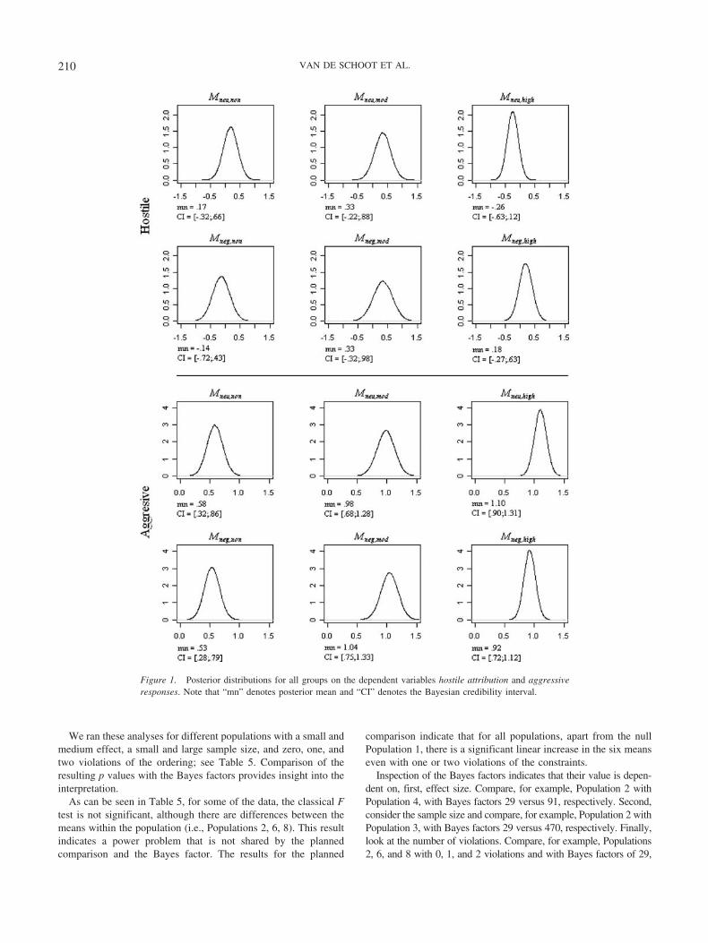
As was correctly noticed by one of the reviewers, it can be illustrativeto provide more information than just the Bayes factors in terms ofmodel fit and model complexity. Information about the posteriordistributions of the means and their credibility intervals can be foundin Figure 1. The interpretation of a Bayesian 95% credibility intervalis that, for example, the posterior probability that Mneu,non for hostileattribution lies in the interval from�.32 to .66 is .95 (see, e.g., Lynch,2007). These intervals are often used in practice to decide whethermeans differ from zero or from other means. It can, for example, beseen that the posterior meanMneu,non for aggression is .58 and that thereis a .95 probability that it is between .32 and .86. This credibilityinterval does not include zero and, consequently, the null hypothesisMneu,non � 0 is rejected. Furthermore, it can be seen that the credi-bility intervals forMneu,non andMneg,non for aggression show an overlap,so the constraint Mneu,non � Mneg,non is not supported by the data.Suppose we observed the same results (i.e., posterior means) but witha larger sample size: The posterior distributions would be morepeaked. Hence, the overlap of the credibility intervals for Mneu,non andMneg,non will disappear. Consequently, the fit of the model wouldincrease. In the next section, we elaborate on the relation betweenmodel fit on one hand, and effect size and sample size on the otherhand.

Bayes Factors Versus p Values

Recall that a Bayes factor provides a direct quantification ofsupport as evidenced in the data for two competing hypotheses.Most researchers would agree that 100 times more support seemsto be quite a lot and, for example, that 1.04 times more support isnot that much. However, clear guidelines are not provided in theliterature, and we do not provide these either. We refrain fromdoing so because we want to avoid creating arbitrary decisionrules. Remember the famous quote about p values: “[. . .] surely,God loves the .06 nearly as much as the .05” (Rosnow &Rosenthal, 1989, p. 1277).To gain insight into the interpretation of Bayes factors in com-

parison with p values, consider the following imaginary example.Suppose there are six means, denoted byM1, . . . , M6, and that theinformative hypothesis of interest is HD: M1 � M2 � M3 � M4 �M5 � M6. We created data in such a way that the sample meansand variance correspond exactly to population values, as shown inFootnote 1 in Table 5. Now let us compare

1. The F test for traditional frequentist analysis,

2. Planned comparisons for thoughtful frequentist analysisassuming a linear increase

� 2.5 � M1 � � 1.5 � M2 � � .5 � M3 � .5 �

M4 � 1.5 � M5 � 2.5 � M6,and

3. Bayesian evaluation of informative hypotheses usingBFs as described above for BFD,unc.

209DIRECTLY EVALUATING EXPECTATIONS

We ran these analyses for different populations with a small andmedium effect, a small and large sample size, and zero, one, andtwo violations of the ordering; see Table 5. Comparison of theresulting p values with the Bayes factors provides insight into theinterpretation.As can be seen in Table 5, for some of the data, the classical F

test is not significant, although there are differences between themeans within the population (i.e., Populations 2, 6, 8). This resultindicates a power problem that is not shared by the plannedcomparison and the Bayes factor. The results for the planned

comparison indicate that for all populations, apart from the nullPopulation 1, there is a significant linear increase in the six meanseven with one or two violations of the constraints.Inspection of the Bayes factors indicates that their value is depen-

dent on, first, effect size. Compare, for example, Population 2 withPopulation 4, with Bayes factors 29 versus 91, respectively. Second,consider the sample size and compare, for example, Population 2 withPopulation 3, with Bayes factors 29 versus 470, respectively. Finally,look at the number of violations. Compare, for example, Populations2, 6, and 8 with 0, 1, and 2 violations and with Bayes factors of 29,

Figure 1. Posterior distributions for all groups on the dependent variables hostile attribution and aggressiveresponses. Note that “mn” denotes posterior mean and “CI” denotes the Bayesian credibility interval.

210 VAN DE SCHOOT ET AL.

20, and 4, respectively. In the latter population there is still support forthe informative hypothesis, but 4 is clearly not a great deal of supportin comparison to the other, much larger, results.Recall the posterior means presented in Figure 1. Suppose the

sample size is increased; then the posterior distributions willbecome more peaked, and the overlap between distributions willdisappear. Stated otherwise, the Bayes factor will increase withincreasing sample size because of an increase in model fit. Thesame holds for an increase in effect size, that is, the further theposterior means are away from each other, the less overlap there isbetween distributions.What can be learned from this exercise? First, Bayes factors are

sensitive for effect size, the number of violations, and sample size.When comparing informative hypotheses, the complexity of eachhypothesis under investigation is independent of these three con-cepts, as we showed before. It is the fit of the model that isinfluenced by the three concepts; in other words, the fit of a modelwill increase with higher effect sizes, a decrease in the number ofviolations, and an increase in sample size. Second, in this sectionwe specified only one single informative hypothesis, which weevaluated with Bayes factors and p values. It is interesting to notethat the Bayes factor tells us exactly how much better a certaininformative hypothesis is against another hypothesis. In compari-son, a p value tells us the probability, given that the null hypothesisis true, of observing the same data or more extreme data than thoseactually observed. The p value, however, is often misinterpreted asthe probability that the null hypothesis is true. Recall that if wewere to specify more informative hypotheses, it would be difficult,or even impossible, to use p values as was shown before.

Conclusion

In this article, we showed how subjective beliefs influenceanalyses in hidden ways and how they might be incorporatedexplicitly. Researchers in developmental psychology often haveexplicit expectations about their research questions, or as Lee andPope (2006) say, “In the real-world much is usually already knownabout a problem before data are collected or observed.” As wehave shown, these expectations can be translated into informativehypotheses. However, as we demonstrated with a case study, theaverage researcher wants to evaluate such informative hypotheses

but tests a set of null hypotheses. We argued that researchersshould not use traditional frequentist analysis, not even thoughtfulfrequentist analysis, if they are not interested in the conclusion thatthe observed data either are or are not in agreement with the nullhypothesis. Rather, researchers should directly evaluate all of theinformative hypotheses under investigation without relying on atest of the null hypothesis. This can be done using Bayesian modelselection. This way, researchers can use all of the knowledgeavailable from previous investigations and can learn more fromtheir data than they can with traditional null hypotheses testing. Allcriticisms of null hypothesis testing aside, the best argument forevaluating informative hypotheses is probably that, like Orobio deCastro et al. (2003), many researchers want to evaluate a set ofhypotheses formulated with inequality constraints but have beenunable to do so because the statistical tools were not yet available.As this article has illustrated, these tools are available to anyresearcher.

References

Achenbach, T. M. (1991). Manual for the Teacher’s Report Form and1991 profiles. Burlington: University of Vermont, Department of Psy-chiatry.

Akaike, H. (1981). Likelihood of a model and information criteria. Journalof Econometrics, 16, 3–14.

Benjamini, Y., & Hochberg, Y. (1995). Controlling the false discoveryrate: A practical and powerful approach to multiple testing. Journal ofthe Royal Statistical Society, Series B, 57, 289–300.

Cohen, J. (1990). Things I have learned (so far). American Psychologist,45, 1304–1312.

Cohen, J. (1992). A power primer. Psychological Bulletin, 112, 155–159.Cohen, J. (1994). The earth is round ( p � . 05). American Psychologist, 49,997–1003.

Coie, J. D., & Dodge, K. A. (1998). Aggression and antisocial behavior. InW. Damon (Series Ed.) & N. Eisenberg (Vol. Ed.), Handbook of childpsychology (5th ed., Vol. 3, pp. 779–862). Toronto, Canada: Wiley.

Dekovic, M., Wissink, I., & Meijer, A. M. (2004). The role of family andpeer relations in adolescent antisocial behaviour: Comparison of fourethnic groups. Journal of Adolescence, 27, 497–514.

Dodge, K. A. (1985). Attributional bias in aggressive children. In P. C.Kendall (Ed.), Advances in cognitive-behavioral research and therapy(pp. 73–110). Orlando, FL: Academic.

Table 5Results of the Comparison Between a Classical F Test, Planned Comparison, and Bayes Factors

PopulationSmall/medium

effectaSmall/large samplesize per group

0/1/2violationsb Classical F test Linear increase

Bayes factor (BF) versusunconstrained model

1 No effectc 100 0 F � 0; p � 1 Contrast � 0; p � 1/2 BF � 1.052 Small 10 0 F � 1.40; p � .15 Contrast � 0.84; p � .01/2 BF � 29.513 Small 100 0 F � 14.0; p � .001 Contrast � 0.84; p � .001 BF � 470.294 Medium 10 0 F � 3.58; p � .007 Contrast � 1.34 p � .001 BF � 91.555 Medium 100 0 F � 35.84; p � .001 Contrast � 1.34; p � .001 BF � 694.276 Small 10 1 F � 1.40; p � .24 Contrast � 0.79; p � .02/2 BF � 20.527 Small 100 1 F � 14.0; p � .001 Contrast � 0.79; p � .001 BF � 48.228 Small 10 2 F � 1.40; p � .23 Contrast � 0.74; p � .02/2 BF � 12.749 Small 100 2 F � 14.0; p � .001 Contrast � 0.74; p � .001 BF � 4.75

a Effect size according to definition of Cohen (1992) with population means for the small effect: �.50, �.30, �.10, .10, .30, .50 (SD � 1; effect size �.11), and for the medium effect:�.80, �.48, �.16, .16, .48, .80 (SD� 1; effect size� .28). b With 1 violation two means are reversed (e.g.,�.50, �.10,�.30, .10, .30,.50) and with 2 violations four means are reversed (e.g. �.50, �.10,�.30, .10, .50, .30). c All means are zero in the population.

211DIRECTLY EVALUATING EXPECTATIONS

Gelman, A.,Carlin, J. B., Stern, H. S., & Rubin, D. B. (2004). Bayesiandata analysis (2nd edition). London: Chapman & Hall.

Hoijtink, H. (1998). Constrained latent class analysis using the Gibbssampler and posterior predictive p-values: Applications to educationaltesting. Statistica Sinica, 8, 691–712.

Hoijtink, H. (2001). Confirmatory latent class analysis: Model selectionusing Bayes factors and (pseudo) likelihood ratio statistics. MultivariateBehavioral Research, 36, 563–588.

Hoijtink, H., Klugkist, I., & Boelen, P. A. (Eds.). (2008). Bayesian eval-uation of informative hypotheses. New York: Springer.

Holm, S. (1979). A simple sequentially rejective multiple test procedure.Scandinavian Journal of Statistics, 6, 65–70.

Howard, G. S., Maxwell, S. E., & Fleming, K. (2000). The proof of thepudding: An illustration of the relative strengths of null hypothesis,meta-analysis, and Bayesian analysis. Psychological Methods, 5, 315–332.

Hsu, J. C. (1996). Multiple comparisons. London: Chapman and Hall.Kammers, M., Mulder, J., De Vignemont, F., & Dijkerman, H. (2009). Theweight of representing the body: Addressing the potentially indefinitenumber of body representations in healthy individuals. ExperimentalBrain Research, 204, 333–342.

Kass, R. E., & Raftery, A. E. (1995). Bayes factors. Journal of theAmerican Statistical Association, 90, 773–795.

Klugkist, I., Laudy, O., & Hoijtink, H. (2005). Inequality constrainedanalysis of variance: A Bayesian approach. Psychological Methods, 10,477–493.

Klugkist, I., Laudy, O., & Hoijtink, H. (2010). Bayesian evaluation ofinequality and equality constrained hypotheses for contingency tables.Psychological Methods, 15, 281–299.

Kuiper, R. M., & Hoijtink, H. (2010). Comparisons of means usingexploratory and confirmatory approaches. Psychological Methods, 15,69–86.

Kuiper, R. M., Klugkist, I., & Hoijtink, H. (2010). A FORTRAN 90program for confirmatory analysis of variance. Journal of StatisticalSoftware, 34, 1–31.

Laudy, O., Boom, J., & Hoijtink, H. (2005). Bayesian computationalmethods for inequality constrained latent class analysis. In A. Van derArk & M. A. C. K. Sijtsma (Eds.), New development in categorical dataanalysis for the social and behavioural sciences (pp. 63–82). London:Erlbaum.

Laudy, O., & Hoijtink, H. (2007). Bayesian methods for the analysis ofinequality constrained contingency tables. Statistical Methods in Medi-cal Research, 16, 123–138.

Lee, M. D., & Pope, K. J. (2006). Model selection for the rate problem: Acomparison of significance testing, Bayesian, and minimum descriptionlength statistical inference. Journal of Mathematical Psychology, 50,193–202.

Lee, M. D., & Wagenmakers, E.-J. (2005). Bayesian statistical inference inpsychology: Comment on Trafimow (2003). Psychological Review, 112,662–668.

Lynch, S. (2007). Introduction to applied Bayesian statistics and estima-tion for social scientists. New York: Springer.

Maxwell, S. E. (2004). The persistence of underpowered studies in psy-chological research: Causes, consequences, and remedies. PsychologicalMethods, 9, 147–163.

Meeus, W., Van de Schoot, R., Keijsers, L., Schwartz, S. J., & Branje, S.(2010). On the progression and stability of adolescent identity formation.A five-wave longitudinal study in early-to-middle and middle-to-lateadolescence. Child Development, 81, 1565–1581.

Meeus, W., Van de Schoot, R., Klimstra, T., & Branje, S. (2010). Changeand stability of personality types in adolescence: A five-wave longitu-dinal study in early-to-middle and middle-to-late adolescence. Manu-script submitted for publication.

Mulder, J., Hoijtink, H., & Klugkist, I. (2009). Equality and inequalityconstrained multivariate linear models: Objective model selection usingconstrained posterior priors. Journal of Statistical Planning and Infer-ence, 140, 887–906.

Mulder, J., Klugkist, I., Van de Schoot, R., Meeus, W. H. J., Selfhout, M.,& Hoijtink, H. (2009). Informative hypotheses for repeated measure-ments: A Bayesian approach. Journal of Mathematical Psychology, 53,530–546.

Orobio de Castro, B., Slot, N. W., Bosch, J. D., Koops, W., & Veerman,J. W. (2003). Negative feelings exacerbate hostile attributions of intentin highly aggressive boys. Journal of Clinical Child and AdolescentPsychology, 32, 56–65.

Orobio de Castro, B., Veerman, J. W., Koops, W., Bosch, J. D., &Monshouwer, H. J. (2002). Hostile attribution of intent and aggressivebehavior: A meta-analysis. Child Development, 73, 916–934.

Rosenthal, R., Rosnow, R. L., & Rubin, D. B. (2000). Contrasts and effectsizes in behavioral research: A correlational approach. Cambridge,England: Cambridge University Press.

Rosnow, R. L., & Rosenthal, R. (1989). Statistical procedures and thejustification of knowledge in psychological science. American Psychol-ogist, 44, 1276–1284.

Schulz, L. E., Bonawitz, E. B., & Griffiths, T. L. (2007). Can being scaredcause tummy aches? Naive theories, ambiguous evidence, and pre-schoolers’ causal inferences. Developmental Psychology, 43, 1124–1139.

Schwarz, G. (1978). Estimating the dimension of a model. Annals ofStatistics, 6, 461–464.

Sober, E. (2002). Bayesianism, its scope and limits. Oxford: Oxford Uni-versity Press.

Van de Schoot, R., Hoijtink, H., & Doosje, S. (2009). Rechtstreeksverwachtingen evalueren of de nul hypothese toetsen? nul hypothesetoetsing versus bayesiaanse model selectie [Directly evaluating expec-tations or testing the null hypothesis: Null hypothesis testing versusBayesian model selection]. De Psycholoog, 4, 196–203.

Van de Schoot, R., Romeijn, J.-W., & Hoijtink, H. (2010). Backgroundknowledge in model selection procedures. Manuscript submitted forpublication.

Van de Schoot, R., & Wong, T. (in press). Do antisocial young adults havea high or a low level of self-concept? Self and Identity.

van Well, S., Kolk, A. M., & Klugkist, I. (2008). The relationship betweensex, gender role identification, and the gender relevance of a stressor onphysiological and subjective stress responses: Sex and gender match andmismatch effects. Behavior Modification, 32, 427–449.

Verhulst, F. C., van der Ende, J., & Koot, H. M. (1997). Handleiding voorde Teacher’s Report Form (TRF): Nederlandse versie [Manual for theTeacher’s Report Form (TRF): Dutch version]. Rotterdam, The Nether-lands: Erasmus Universiteit Rotterdam.

Wagenmakers, E.-J. (2007). A practical solution to the pervasive problemsof p -values. Psychonomic Bulletin & Review, 14, 779–804.

Wainer, H. (1999). One cheer for null hypothesis significance testing.Psychological Methods, 4, 212–213.

Walker, L. J., Gustafson, P., & Frimer, J. A. (2007). The application ofBayesian analysis to issues in developmental research. InternationalJournal of Behavioral Development, 31, 366–373.

Walker, L. J., Gustafson, P., & Hennig, K. H. (2001). The consolidation/transition model in moral reasoning development. Developmental Psy-chology, 37, 187–197.

Received September 9, 2008Revision received July 5, 2010

Accepted July 8, 2010 �

212 VAN DE SCHOOT ET AL.