This is a preprint of an article accepted for publication in Journal of Fore-

casting Copyright c© 2002.

1

Selection of Value-at-Risk models∗†

Mandira Sarma ‡ Susan Thomas Ajay Shah

May 2, 2001

∗This is a preprint of an article accepted for publication in Journal of Forecasting Copyright c© 2002.†An earlier draft of this paper was presented at the Money, Macro and Finance Conference 2000 (South Bank

University, London), the International Conference of the Royal Statistical Society 2000 (University of Reading,Reading), the SIRIF conference on Value-at-Risk (Edinburgh, Scotland), and the 7th Annual Meeting of theGerman Finance Association and Conference on Intertemporal Finance (University of Konstanz, Germany).We thank the participants of these conferences for helpful comments and suggestions. We also thank PeterChristoffersen for his useful comments. All errors are ours.‡Corresponding author: Mandira Sarma, Indira Gandhi Institute of Development Research, Goregaon

(East), Mumbai 400 065. Phone: +91-22-840-0919. Fax: +91-22-840-2752. Email: mandira@igidr.ac.in

2

Abstract

Value-at-Risk (VaR) is widely used as a tool for measuring the market risk of asset

portfolios. However, alternative VaR implementations are known to yield fairly different

VaR forecasts. Hence, every use of VaR requires choosing amongst alternative forecasting

models.

This paper undertakes two case studies in model selection, for the S&P 500 index

and India’s NSE-50 index, at the 95% and 99% levels. We employ a two-stage model

selection procedure. In the first stage we test a class of models for statistical accuracy.

If multiple models survive rejection with the tests, we do a second stage filtering of the

surviving models using subjective loss functions. This two-stage model selection procedure

does prove to be useful in choosing a VaR model, while only incompletely addressing the

problem. These case studies give us some evidence about the strengths and limitations of

present knowledge on estimation and testing for VaR.

KEY WORDS model selection; Value-at-Risk; conditional coverage; loss functions

JEL Classification: C22, C52, G10, G28

3

1 Introduction

Value-at-Risk (VaR) is a measure of the market risk of a portfolio. It quantifies, in monetary

terms, the exposure of a portfolio to future market fluctuations. The concept of VaR as a tool

for risk measurement has been widely accepted in the finance profession. While the concept

is simple and attractive, there is no unique path which VaR implementations adopt. There

are a wide variety of alternative models which are used in VaR implementations, and every

real–world application of VaR is faced with the need to choose amongst these alternatives.

This is a non-trivial problem, since it has been found that different methodologies can yield

different Value-at-Risk measures for the same portfolio, sometimes leading to significant er-

rors in risk measurement. The risk of faulty risk management owing to deficiencies of the

underlying models is called “model risk”, and is recognised as an important issue in risk

management. This has led to a heightened interest in measuring the quality of alternative

VaR implementations, and in the problem of model selection.

One way to address this question is to do statistical hypothesis testing, in order to test

whether the VaR measures coming out from alternative models display the required theoretical

properties. An alternative approach is to define loss functions reflecting the loss from the

failure of a particular model to a particular risk manager. This approach emphasises the role

of the utility function of the risk manager: regulators may have very different utility functions

in this context as compared with firms, and a hedge fund may have a utility function which is

unlike that of a bank. The loss function approach integrally incorporates the risk manager’s

preferences into the model selection process.

In this paper we have employed a two stage VaR model selection framework, where testing

for statistical accuracy precedes measuring the loss to the economic agent using the model.

The first stage of the model selection process involves testing the competing VaR models for

statistical accuracy. A well specified VaR model should produce statistically meaningful VaR

forecasts. The basic feature of a 99% VaR is that it should be exceeded 1% of the time,

and that the probability of the VaR being exceeded at time t + 1 remains 1% even after

4

conditioning on all information known at time t. This implies that the VaR should be small

in times of low volatility and high in times of high volatility, so that the events where the loss

exceeds the forecasted VaR measure are spread over the entire sample period, and do not come

in clusters. A model which fails to capture the volatility dynamics of the underlying return

distribution will exhibit the symptom of clustering of failures, even if (on the average) it may

produce the correct unconditional coverage. The first stage of the model selection process

involves testing the VaR measures produced by different models for “conditional coverage”

(Christoffersen, 1998; Christoffersen and Diebold, 2000).

In the second stage of the evaluation process, certain “loss functions” are defined depend-

ing upon the utility function of the risk manager. The VaR model which maximises utility

(minimises loss) is considered attractive. In this paper we consider two loss functions: the

“regulatory loss function” and the “firm’s loss function”. The regulatory loss function ex-

presses the goals of a financial regulator and the firm’s loss function additionally measures

the opportunity cost of capital faced by the firm. A non parametric sign test has been used to

test for the superiority of a VaR model vis-a-vis another in terms of the loss function values.

We apply this two stage methodology to a class of 15 models of VaR estimation for two

prominent equity indices, the S&P 500 and India’s ‘Nifty’ index.

Our results highlight the limitations of present knowledge in VaR estimation and testing.

In the case of the S&P 500 index, all 15 models are rejected at the first stage (for 99% as

well as 95% level). In the case of the NSE-50 index for 95% VaR estimation, a statistically

appropriate model could be chosen in the first stage itself, while at 99% level, two models were

accepted in the first stage and we applied the second stage of filtering to the two competing

models, by using the loss functions reflecting the risk management problems of a regulator

and a firm.

Our proposed two–stage model selection procedure does help in reducing to a smaller set of

competing models, but it may not always uniquely identify one model. In such cases, other

real–world considerations, such as computational cost, might be applied to favour one model.

5

The rest of this paper is organised as follows. Section 2 presents the problems of VaR esti-

mation. Section 3 describes the first stage of the model selection process. Section 4 describes

the “loss function” approach and the loss functions that are used in this paper. The empirical

work is presented in Section 6 along with the major findings, and Section 7 concludes the

paper.

2 Issues in model selection

Let rt be the change in the value of a portfolio over a certain horizon, and let rt ∼ ft(r). The

VaR vt at a (1− p) level of significance is defined by :

∫ vt

−∞ft(r)dr = p

We define a ‘failure’ as an outcome rt < vt. Intuitively, a “good” VaR estimator vt would be

such that that Pr(rt < v̂t) is always “close” to p.

There is an extensive literature on estimators of vt, including methods such as the variance–

covariance approach, historical simulation, and techniques based on extreme value theory

(Jorion, 1997; Jordan and Mackay, 1997).1 VaR estimates obtained through alternative

methodologies prove to have economically significant differences (Beder, 1995; Hendricks,

1996). Given the existence of these alternative models for VaR estimation, and the impor-

tance of VaR to financial firms and financial regulators, evaluating the validity and accuracy

of such measures has become an important question. Every use of VaR in a real–world setting

faces the problem of choosing one amongst the alternative estimators, ranging from a variety

of structural models to model–free simulations.

There is a recent, and rapidly growing, literature on the evaluation of VaR models. From

a regulatory perspective, it is highly desirable to treat the VaR model as a black–box, and1Also see Danielsson and de Vries (1997, manuscript, London School of Economics); McNeil and Saladin

(1997, manuscript, Department Mathematik, ETH Zentrum, Zurich).

6

obtain inferences about its quality using the observed time–series of rt and vt. Strategies

for testing and model selection are said to be “model–free” if the information set that they

exploit is restricted to the time–series of rt and vt.

The literature dates back to Kupiec (1995) who offered a testing framework based on certain

theoretical properties of the VaR measures. These tests ignore conditional coverage, and

Kupiec finds that these tests have poor statistical power. Crnkovic and Dranchman (1996)

developed a testing methodology which incorporates the conditional coverage aspect, but is

not model–free. Berkowitz (1999) offered a powerful testing framework which is well suited

for samples, without being model–free.

The testing methodology developed by Christoffersen (1998) focuses on the essence of the

VaR estimation problem – that we should observe failures with probability p after taking

into account all conditioning variables. Christoffersen’s test is based on testing whether

Pr(rt < vt) = p after conditioning on all information available at time t. This methodology

is model–free, in that it only requires a time–series of the failure events. Christoffersen’s

original methodology offered an incomplete test for the correct conditional coverage. This

led to the work of Christoffersen and Diebold (2000) and Clements and Taylor (2000)2 on

improved tests for correct conditional coverage.

Tests of conditional coverage can be viewed as a necessary condition for a well specified

VaR forecasting procedure. However, we often find that multiple alternative models are not

rejected by such tests. In this situation, we turn to decision theory to assist in choosing a

VaR estimator. This is related to a significant literature on the role for the utility function

in forecasting (Granger and Pesaran, 2000).

One aspect of this is the importance of asymmetric utility functions. West et al. (1993) find

that in the context of model selection for models of exchange rate volatility, decision theory is

particularly relevant when utility functions are asymmetric. This is pertinent for our present

context, i.e. the use of VaR models in the risk management profession. Events where rt < vt2Clements MP and Taylor N, 2000. Evaluating interval forecasts of high-frequency financial data.

Manuscript, University of Warwick.

7

are particularly important in the eyes of the risk manager. Both the utility functions that we

specify – that of the regulator and that of the firm – exhibit asymmetry.3

We use a two–stage model selection strategy where, in the second stage, loss functions are used

to to choose the VaR model which yields the least loss amongst this set. Firms and regulators

use VaR for different purposes – for capital allocation (which generates opportunity cost),

for supervision of traders, or for capping the insolvency probability of firms, etc. We try to

specify loss functions which reflect the risk management problem at hand and then choose

the VaR model which generates the least loss. This approach is discussed in Section 4.

3 Statistical tests

A correctly specified VaR model should generate the pre specified failure rate conditionally

at every point in time. This is known as the property of “conditional coverage” of the VaR

model.

In an important paper, Christoffersen (1998) developed a framework for ‘interval forecast

evaluation’. The VaR is interpreted as a forecast that the portfolio return will lie in (−∞, vt]

with a pre specified probability p. Christoffersen emphasises testing the “conditional cover-

age” of the interval forecasts. The importance of testing “conditional” coverage arises from

the observation of volatility clustering in many financial time–series. Good interval forecasts

should be narrow in tranquil times and wide in volatile times, so that the observations falling

outside a forecasted interval are spread over the entire sample, and do not come in clusters.

A poor interval forecast may produce correct unconditional coverage, yet it may fail to ac-

count for higher-order time dynamics. In this case, the symptom that would be observed is

a clustering of failures.

Consider a sequence of one period ahead VaR forecasts {vt|t−1}Tt=1, estimated at a significance

level 1− p. These forecasts are intended to be one–sided interval forecasts (−∞, vt|t−1] with3A related question consists of asking how the utility function should be explicitly exploited in VaR esti-

mation itself. This is related to the work of Weiss (1996) in the context of forecasting. We do not address thisaspect in this paper.

8

coverage probability p. Given the realisations of the return series rt and the ex-ante VaR

forecasts, the following indicator variable may be defined

It =

{ 1 if rt < vt

0 otherwise

The stochastic process {It} is called the “failure process”. The VaR forecasts are said to

be efficient if they display “correct conditional coverage”, i.e., if E[It|t−1] = p ∀ t. This is

equivalent to saying that the {It} series is iid with mean p.

To test for the “correct conditional coverage”, Christoffersen develops a three step testing

procedure: a test for “correct unconditional coverage”, a test for “independence”, and a

test for “correct conditional coverage”. In the test for “correct unconditional coverage”,

the null hypothesis of the failure probability p is tested against the alternative hypothesis

that the failure probability is different from p, under the assumption of an independently

distributed failure process. In the test for “independence”, the hypothesis of an independently

distributed failure process is tested against the alternative hypothesis of a first order Markov

failure process. Finally, the test of “correct conditional coverage” is done by testing the null

hypothesis of an independent failure process with failure probability p against the alternative

hypothesis of a first order Markov failure process with a different tpm.

All the three tests are carried out in the likelihood ratio (LR) framework. The likelihood

ratio statistic for each is as follows:

1. LR statistic for the test of “unconditional coverage”:

LRuc = −2 log[ pn1(1− p)n0

π̂n1(1− π̂)n0

]∼ χ2

(1)

where

9

p = Tolerance level at which VaR measures are estimated

n1 = Number of 1’s in the indicator series

n0 = Number of 0’s in the indicator series

π̂ =n1

n0 + n1, the MLE of p

2. LR statistic for the test of independence:

LRind = −2 log(1− π̂2)(n00+n10)π̂

(n01+n11)2

(1− π̂01)n00 π̂n0101 (1− π̂11)n10 π̂n11

11

∼ χ2(1)

where

nij = Number of i values followed by a j value in the It series

(i, j = 0, 1)

πij = Pr{It = i|It−1 = j} (i, j = 0, 1)

π̂01 =n01

n00 + n01

π̂11 =n11

n10 + n11

π̂2 =n01 + n11

n00 + n01 + n10 + n11

3. LR statistic for the test of “correct conditional coverage”:

LRcc = −2 log(1− p)n0pn1

(1− π̂01)n00 π̂n0101 (1− π̂11)n10 π̂n11

11

∼ χ2(2)

If we condition on the first observation, then these LR test statistics are related by the identity

10

LRcc = LRuc + LRind.

Christoffersen’s basic framework is limited in that it only deals with first order dependence

in the {It} series. It would fail to reject an {It} series which does not have first order

Markov dependence but does exhibit some other kind of dependence structure (e.g., higher

order Markov dependence or periodic dependence). Two recent papers, Christoffersen and

Diebold (2000) and Clements and Taylor (2000), generalise this. These papers suggest that a

regression of the It series on its own lagged values and some other variables of interest, such as

day-dummies or the lagged observed returns, can be used to test for the existence of various

form of dependence structures that may be present in the {It} series. Under this framework,

conditional efficiency of the It process can be tested by testing the joint hypothesis:

H : Φ = 0, α0 = p (1)

where

Φ = [α1, ...αS , µ1, ..., µS ]′

in the regression

It = α0 +S∑s=1

αsIt−s +S−1∑s=1

µsDs,t + εt (2)

t = S + 1, S + 2, ..., T (3)

Ds,t are explanatory variables. (4)

The hypothesis (1) can be tested by using an F-statistic in the usual OLS framework.4

4In view of the fact that the It series is binary, a more appropriate way is to do a binary regression ratherthan an OLS regression. However, there seem to be a technical problem in the implementation of the binaryregression as more than 90% of the It’s are zero and only a few are unity. This asymmetry in the data

11

It should be noted that there is no one–to–one correspondence between the Christoffersen

(1998) test and the regression based test. While one can expect that a model rejected by the

Christoffersen (1998) test would also be rejected by the regression based test, this does not

necessarily have to be so. In this paper, we reject a model if it is rejected by either of these

two tests.

4 Loss functions

The idea of using loss functions as a means of evaluating VaR models was formalised by

Lopez (1998, 1999). Under this approach, loss functions reflecting specific concerns of the

risk managers are defined. Such loss functions are defined with a negative orientation – they

give higher scores when failures take place. VaR models are assessed by comparing the values

of the loss function. A model which minimises the loss is preferred over the other models.

As an illustration, consider the simplest loss function – the binomial loss function. Here a

score of 0 is attached to the loss function when It = 0 (i.e. when a success occurs) and a score

of 1 is attached when It = 1 (i.e. when a failure occurs). It is possible to treat this as a loss

function and identify the VaR estimation procedure which minimises this. This is effectively

the same as the estimated unconditional coverage in Christoffersen’s test. However, it is hard

to imagine an economic agent who has such a utility function: one which is neutral to all

It = 0 events, which abruptly shifts to It = 1 in the slightest failure, and penalises all failures

equally. Therefore, we need to think more closely about the utility functions of risk managers

in the evaluation of alternative VaR estimators.

Lopez proposed three loss functions which might reflect the utility function of a regulator:

the binomial loss function, the magnitude loss function and the zone loss function. Broadly

speaking, the latter two penalise failures more severely as compared with the binomial loss

function.

results in singular Hessian matrices in the estimation process and the maximum likelihood estimation fails asa result. This problem seems to be more severe in the case of 99% VaR models. Therefore we resort to anOLS regression, which is asymptotically equivalent to a binary regression.

12

The example above, which highlights the shortcomings of the binomial loss function, is per-

suasive insofar as it motivates a role for the utility function of the risk manager in the model

selection process. However, actually specifying the utility function of a real–world risk man-

ager is difficult. As in other applications of statistical decision theory, there is an element of

arbitrariness in writing down the utility function. In this paper we write down a “regulatory

loss function” to reflect the regulator’s utility function, and a “firm’s loss function” which

reflects the utility function of a firm. As with any application of loss functions, this approach

is vulnerable to mis-specification of the loss function.

4.1 Regulatory loss function (RLF)

The rlf that we use is similar to the “magnitude loss function” of Lopez (1998). It penalises

failures differently from the binomial loss function, and pays attention to the magnitude of

the failure.

lt =

{ (rt − vt)2 if rt < vt

0 otherwise

The quadratic term in the above loss function ensures that large failures are penalised more

than the small failures.

4.2 The firm’s loss function (FLF)

Firms use VaR in internal risk management. Here, there is a conflict between the goal of safety

and the goal of profit maximisation. A VaR estimator which reported “too high” values of

VaR would force the firm to hold “too much” capital, imposing the opportunity cost of capital

upon the firm. We propose to model the firm’s loss function by penalising failures (much like

the rlf) but also imposing a penalty reflecting the cost of capital suffered on other days. We

define the flf as follows:

13

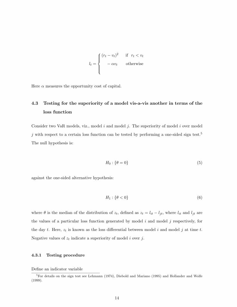
lt =

(rt − vt)2 if rt < vt

− αvt otherwise

Here α measures the opportunity cost of capital.

4.3 Testing for the superiority of a model vis-a-vis another in terms of the

loss function

Consider two VaR models, viz., model i and model j. The superiority of model i over model

j with respect to a certain loss function can be tested by performing a one-sided sign test.5

The null hypothesis is:

H0 : {θ = 0} (5)

against the one-sided alternative hypothesis:

H1 : {θ < 0} (6)

where θ is the median of the distribution of zt, defined as zt = lit − ljt, where lit and ljt are

the values of a particular loss function generated by model i and model j respectively, for

the day t. Here, zt is known as the loss differential between model i and model j at time t.

Negative values of zt indicate a superiority of model i over j.

4.3.1 Testing procedure

Define an indicator variable5For details on the sign test see Lehmann (1974), Diebold and Mariano (1995) and Hollander and Wolfe

(1999).

14

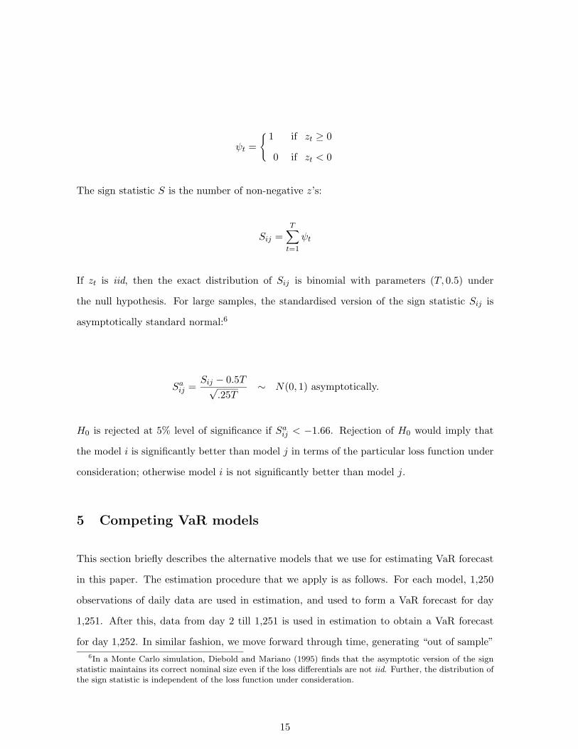
ψt =

{ 1 if zt ≥ 0

0 if zt < 0

The sign statistic S is the number of non-negative z’s:

Sij =T∑t=1

ψt

If zt is iid, then the exact distribution of Sij is binomial with parameters (T, 0.5) under

the null hypothesis. For large samples, the standardised version of the sign statistic Sij is

asymptotically standard normal:6

Saij =Sij − 0.5T√

.25T∼ N(0, 1) asymptotically.

H0 is rejected at 5% level of significance if Saij < −1.66. Rejection of H0 would imply that

the model i is significantly better than model j in terms of the particular loss function under

consideration; otherwise model i is not significantly better than model j.

5 Competing VaR models

This section briefly describes the alternative models that we use for estimating VaR forecast

in this paper. The estimation procedure that we apply is as follows. For each model, 1,250

observations of daily data are used in estimation, and used to form a VaR forecast for day

1,251. After this, data from day 2 till 1,251 is used in estimation to obtain a VaR forecast

for day 1,252. In similar fashion, we move forward through time, generating “out of sample”6In a Monte Carlo simulation, Diebold and Mariano (1995) finds that the asymptotic version of the sign

statistic maintains its correct nominal size even if the loss differentials are not iid. Further, the distribution ofthe sign statistic is independent of the loss function under consideration.

15

VaR estimates. For each dataset, this is done for each of the 15 VaR models described here.

1. The equally weighted moving average (ewma) model.

Under this model, the standard deviation of returns for date t is estimated over a window

from date t− k till date t− 1:

σt =

√√√√ 1(k − 1)

t−1∑s=t−k

r2s

The returns are assumed to be normally distributed, so the VaR estimates are obtained

using percentile points on the normal distribution: the 99% VaR is −2.33σt and the

95% VaR is −1.66σt.

In this procedure, the choice of window width k is critical. Short windows suffer from

inferior statistical efficiency, however they do better in capturing short–term volatility

dynamics. We report results for five window widths: 50, 125, 250, 500 and 1,250 days.7

2. The RiskMetrics (rm) model.

The RiskMetrics model J.P.Morgan/Reuters (1996) proposes an alternative estimator

of σt:

σt =

√√√√(1− λ)t−1∑s=t−k

λ(t−s−1)r2s

=√λσ2

t−1 + (1− λ)r2t−1

Once σt is estimated, the VaR is estimated under the assumption that returns are

normally distributed, as in the case of (ewma).

Here, λ ∈ (0, 1) is known as the decay factor, which reflects how the impact of past7Regardless of the window width, in all cases, we have exactly the same number of “out of sample” VaR

estimates. Suppose a window width of 50 days is used. Then the first VaR estimate (for date 1251) uses astandard deviation estimated from observations 1201 till 1250.

16

observations decays while forecasting one–day ahead σt. The most recent observation

has the largest impact and the impact decays exponentially, as the observations move

towards the past. With a low value of λ, the weight attached to historical returns decays

rapidly as we go further into the past. A high λ, on the other hand leads to a much

lower decay of the weights and thus indicate a longer memory of the past observations.

VaR estimates obtained using RiskMetrics are more variable for small values of λ.

Through this, the RiskMetrics procedure takes cognisance of the volatility cluster-

ing which has often been observed with financial time–series. Even at λ = 0.99, the

RiskMetrics estimates are more sensitive to recent observations than the (ewma) with

k = 1250: this is because 0.991250 is 3.5 × 10−2 whereas under the ewma(1250), the

oldest observation would have a weight of 8× 10−4.

The value λ = 0.94 has been widely used by J. P. Morgan and was recommended by the

Varma Committee in India. We have used four different values of λ for VaR estimation,

viz. λ = 0.90, 0.94, 0.96 and 0.99.

3. The garch model.

This uses the class of models developed by Engle (1982) and Bollerslev (1986). As with

the ewma and the rm models, the return series is assumed to be conditionally normally

distributed and VaR measures are calculated by multiplying the conditional standard

deviation by the appropriate percentile point on the normal distribution.

We have used an ar(1)-garch(1,1) for estimating the conditional volatility:8

rt = α0 + α1rt−1 + εt

ε ∼ N(0, σ2t )

σt =√γ0 + γ1ε2t−1 + γ2σ2

t−1

8The AR(1) term is included because we found significant AR(1) coefficients for both the portfolios underconsideration in this paper.

17

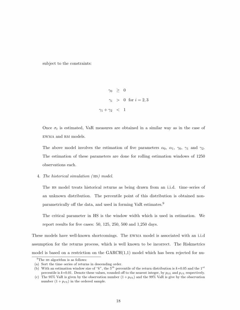
subject to the constraints:

γ0 ≥ 0

γi > 0 for i = 2, 3

γ1 + γ2 < 1

Once σt is estimated, VaR measures are obtained in a similar way as in the case of

ewma and rm models.

The above model involves the estimation of five parameters α0, α1, γ0, γ1 and γ2.

The estimation of these parameters are done for rolling estimation windows of 1250

observations each.

4. The historical simulation ( hs) model.

The hs model treats historical returns as being drawn from an i.i.d. time–series of

an unknown distribution. The percentile point of this distribution is obtained non-

parametrically off the data, and used in forming VaR estimates.9

The critical parameter in HS is the window width which is used in estimation. We

report results for five cases: 50, 125, 250, 500 and 1,250 days.

These models have well-known shortcomings. The ewma model is associated with an i.i.d

assumption for the returns process, which is well known to be incorrect. The Riskmetrics

model is based on a restriction on the GARCH(1,1) model which has been rejected for nu-9The hs algorithm is as follows:

(a) Sort the time–series of returns in descending order.(b) With an estimation window size of “k”, the 5th percentile of the return distribution is k∗0.05 and the 1st

percentile is k∗0.01. Denote these values, rounded off to the nearest integer, by p5% and p1% respectively.(c) The 95% VaR is given by the observation number (1 + p5%) and the 99% VaR is give by the observation

number (1 + p1%) in the ordered sample.

18

merous financial time-series, including the time-series used in this paper. The GARCH(1,1)

model is widely employed in the literature, though certain blemishes are fairly well known,

in particular with respect to difficulties of aggregation and persistence. Finally, historical

simulation is based on an i.i.d. assumption which is known to be incorrect.

We proceed with a case study of model selection with this weak set of models for two reasons.

First, we expect that powerful tests of VaR models should be effective in rejecting many of

these weak models. Second, these weak models are widely used in the real–world, and it is

useful to obtain feedback about their quality.

6 Empirical application

In this section, we present a set of case studies where these ideas are applied for model selection

in a class of standard models for 95% and 99% VaR estimation for two stock market indexes:

a long position on the S&P 500 and the S&P CNX Nifty (of India). Roughly speaking, in

both cases, we work with around 2,500 observations of daily returns from July 1990 through

July 2000.10

6.1 Model selection for 95% VaR

6.1.1 95% VaR for S&P 500

Christoffersen (1998) test. Table 1 provides the results of the Christoffersen (1998) test

for 95% VaR estimation for the S&P 500 portfolio.

[Table 1 about here.]10We use 2,534 daily logarithmic returns on the S&P 500 portfolio from 3 July, 1990 till 31 July, 2000.

The first 1,250 observations (from 3 July 1990 till 29 June, 1995) are used for estimating one day ahead VaRforecasts for the period 30 June, 1995 till 31 July 2000. This gives us 1,283 “out–of–sample” VaR forecasts forapplying our model selection procedure.

For the Nifty portfolio we use 2,391 daily logarithmic returns from 3 July 1990 till 6 December 2000. Thefirst 1,250 observations (from 3 July 1990 till 7 May 1996) comprise the estimation window and the rest of 1141observations (from 8 May 1996 till 6 December 2000) are used for making “out–of–sample” VaR forecasts.

19

Most often, we find that the normal distribution based models are not rejected, while the

historical simulation models are rejected quite often. Among the normal distribution based

models, Christoffersen’s test rejects ewma(500) and ewma(1250). On the other hand all

the hs models except hs(125) are rejected. Interestingly, all these models are rejected for

lacking the property of “correct unconditional coverage”, though they all are found to satisfy

the “independence” property (in the first order sense).

It is interesting to note that for the acceptable models, p̂ and π̂11 are approximately equal.

For the models which are rejected for not having the property of “correct coverage”, p̂ is

significantly different from the theoretical value of 0.05.

Higher order dependence. The next step of the statistical testing procedure is to perform

a test for the existence of higher order and/or periodic dependence on the models. We consider

two types of dependence structures:

1. Lagged dependence upto an order of five, and

2. Periodic dependence in the form of a day-of-the-week effect.

We perform an OLS regression of the It series on its five lagged values and five day–dummies

representing the trading days in a week. Significance of the F-statistic of this OLS will lead

to rejection of a model; otherwise it will lead to its non-rejection. It should be noted that

the non-significance of the F-statistic does not necessarily imply non-significance of the t-

statistics corresponding to the individual regressors in the OLS. We follow Hayashi (2000)

(page 44) and adopt the policy of preferring the F-statistic over the t-statistic(s) in the case

of a conflict. Therefore a model will not be rejected if the F-statistic is not significant even

though some individual t-statistic(s) may turn out to be significant.

Table 2 presents the results of the regression based tests for all the models of 95% VaR

estimation for the S&P 500 portfolio. The first column of this table gives the names of the

models, the second column reports the value of the F-statistics for testing the hypothesis

(1), the third column gives the corresponding p-values and the fourth column reports which

individual regressors, if any, are found significant in the OLS regression.

20

[Table 2 about here.]

For the S&P 500 portfolio, the F-statistic is found to be significant at 0.05 level for all the 15

models. This means that none of these models are able to produce a failure series which is iid,

and therefore all these models may be rejected as statistically flawed for estimating 99% VaR

estimates for the S&P 500 index. A closer look at the fourth column of the table 2 reveals

that these models exhibit significant second order Marcov dependence. The model hs(125)

exhibits a fifth order dependence as well.The models rm(.94) and rm(.96) also indicate the

presence of a significant “Wednesday” effect.

We see that the models which were not rejected by the Christoffersen (1998) test are rejected

by the regression based test. This is due to the fact that Christoffersen (1998) test is not

capable of rejecting a model which does not have first order dependence but does have higher

order (in this case second order) or periodic dependence (in this case Wednesday effect).

6.1.2 95% VaR for S&P CNX Nifty

Christoffersen (1998) test. For the Nifty portfolio, for 95% VaR estimation, the Christof-

fersen (1998) test rejects ewma(50), ewma(500), all the hs models except hs(1250), and

all the RiskMetrics models except RiskMetrics (.90) (Table 3). Among the rejected models,

all except the hs(50) lack the property of “independence”, while hs(50) lacks the property

of “correct unconditional coverage”. The model hs(500) is rejected on both counts.

[Table 3 about here.]

Higher order dependence. We perform an OLS regression of the failure process generated

by each model on five lagged values of the failure process and five day–dummies. The results

are presented in Table 4. The regression tests reject all but ar(1)-garch(1,1). The rejected

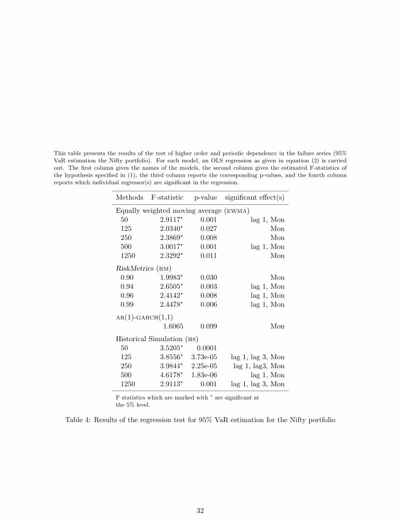
models exhibit the existence of significant lagged and “Monday” effects in the failure process.

The models which were rejected by Christoffersen (1998) test for the It process lacking “first

order Markov independence” property are found to be rejected on the same ground as well as

for having significant “Monday” effects, and in some cases a third order lagged dependence.

21

[Table 4 about here.]

At the end of the first stage of the model selection process, we are left with ar(1)-garch(1,1),

as the best model. Since this is the uniquely determined model, therefore we do not need to

proceed to the second stage of the model selection process, and infer that ar(1)-garch(1,1)

is the most appropriate model which can generate statistically meaningful 95% VaR measures

for the Nifty index.

6.2 Model selection for 99% VaR

6.2.1 99% VaR for S&P 500

Christoffersen (1998) test. The results of the Christoffersen (1998) test applied for 99%

VaR estimation for the S&P 500 portfolio (Table 5) are striking: each of the 15 models is

rejected. In this case, none of the models is found to possess the property of “correct coverage”

while all of them possess the “independence” property (in the first order sense). Thus, every

model that we have considered here underestimates the risk at a 99% significance level; i.e.,

the p̂ values for all the models are well above 0.01.

[Table 5 about here.]

Higher order dependence. The results of the regression tests for 99% VaR estimation for

the S&P 500 portfolio are shown in Table 6. All the models are found to have an α coefficient

which is significantly different from the hypothetical value 0.01. This was also confirmed

by Christoffersen’s test as the LR test of “unconditional coverage” was rejected for all the

models. Apart from this, we find a significant Wednesday effect in the It series for most of

the models. We can also see lagged effects of order 1 and 2 for some models.

[Table 6 about here.]

Thus, at the end of the first stage, we do not have any appropriate model for 99% VaR

estimation for the S&P 500 portfolio.

Hence, we do not proceed further to the second stage of the model selection procedure.

22

6.2.2 99% VaR for S&P CNX Nifty

Christoffersen (1998) test. Table 7 presents the results of Christoffersen’s test for 99%

VaR estimation for the Nifty portfolio. Christoffersen’s test rejects ewma(500), ewma(1250)

and all the hs models except hs(500). All these models have been rejected for not having

the “correct unconditional coverage”.

[Table 7 about here.]

Higher order dependence. The results of the regression based test for higher order and

periodic dependence in the failure process are shown in Table 8. The regression tests indicate

that most of the models indicate significant “Monday” effects in the failure processes produced

by them. Some of the models also indicate the presence of significant lagged dependence of

orders 4 and 1 in the failure processes. The F-statistics for two models, viz. the models

rm(.90) and ar(1)-garch(1,1) are found to be insignificant. Therefore both of these models

may be considered appropriate in terms of statistical accuracy of the 99% VaR estimates that

they are producing for the Nifty index.

[Table 8 about here.]

Are these two statistically equivalent models economically equivalent as well? To answer

this question we go to the second stage of the model selection process, where loss functions

reflecting two different risk management problems are calculated and tested to choose a model

which minimises the losses due to risk management.

Loss functions. Table 9 presents the summary results of the “loss function approach”

applied to the models rm(.90) and ar(1)-garch(1,1) which are found to be “acceptable”

in the first stage of the model selection procedure. The first column of the table pertains

to the “regulatory loss function” (rlf) and the second column pertains to the “firm’s loss

function” (flf). The Panel A of the table reports the average values of the two loss functions

produced by rm(.90) and ar(1)-garch(1,1). These values indicate that ar(1)-garch(1,1)

produces lower economic losses, both for a regulator and for a firm. To test whether the losses

are statistically significantly different, we carry out the nonparametric sign test described in

23

Section 4.3.

Panel B of Table 9 reports the values of the standerdised sign statistic given in Section 4.3.1.

The sign tests applied to the rlf values for rm(.90) and ar(1)-garch(1,1) implies that the

two models are not significantly different from each other. Therefore, as far as the specific

rlf is concerned, both of them may be considered equivalent. Hence, a financial regulator

would remain indifferent between these two models with respect to the rlf considered here.

The sign test applied to these models with respect to the flf shows that rm(.90) is signifi-

cantly better than ar(1)-garch(1,1). Therefore, it may be considered the best model for a

firm having this specific loss function.

[Table 9 about here.]

6.3 Summarising these results

[Table 10 about here.]

Table 10 summarises these four case studies. In each case, we started with 15 models. The

table shows the survivors left with the Christoffersen (1998) test, after regression–based test

for higher-order dependence in the It series, and the preferred model(s) amongst these based

on the loss function of the firm or the regulator.

7 Conclusion

In this paper we set out to think about how a VaR model should be selected. We view

statistical accuracy as a necessary condition: models which do not have the property of

“correct conditional coverage” are statistically flawed and should not be used. We use existing

first–order and regression based tests for the existence of “correct conditional coverage”.

There may be cases where more than a single model satisfy the property of “correct conditional

coverage” (as in the case of the Nifty portfolio for 99% VaR estimation in this paper). It is

useful to bring the utility function of the risk manager into the picture at this point. In

24

the light of the utility function of the risk manager, we are often able to find economically

significant differences between two VaR models, both of which have the correct conditional

coverage.

In general, our model selection procedure does help in reducing to a smaller set of competing

models, but it may not always uniquely identify one model. In such cases, other real–world

considerations such as, computational cost, might be applied to favour one model.

25

References

Beder TS, 1995 Sept Oct. VAR: Seductive but Dangerous. Financial Analysts Journal 12–23.

Berkowitz J, 1999 March. Evaluating the Forecasts of Risk Models. Federal Reserve Board.

Bollerslev T, 1986. Generalized Autoregressive Conditional Heteroskedasticity. Journal of

Econometrics 31:307–327.

Christoffersen PF, 1998. Evaluating Interval Forecasts. International Economic Review

39:841–862.

Christoffersen PF, Diebold FX, 2000. How Relevant is Volatility Forecasting for Financial

Risk Management. Review of Economics and Statistics 82:1–11.

Crnkovic C, Dranchman J, 1996. Quality Control. Risk 9(9):138–143.

Diebold FX, Mariano R, 1995 July. Comparing Predictive Accuracy. Journal of Business

and Economic Statistics 13(3):253–263.

Engle R, 1982 July. Autoregressive Conditional Heteroscedasticity with Estimates of the

Variance of United Kingdom Inflation. Econometrica 50:987–1007.

Granger CWJ, Pesaran MH, 2000. Economic and Statistical Measures of Forecast Accuracy.

Journal of Forecasting 19:537–560.

Hayashi F, 2000. Econometrics. Princeton Univ Press.

Hendricks D, 1996. Evaluation of Value at Risk Models for Historical Data. Federal Reserve

Bank of New York Economic Policy Review 2(1):49–69.

Hollander M, Wolfe DA, 1999. Nonparametric statistical methods. John Wiley, New York,

2nd edn.

Jordan JV, Mackay RJ, 1997. Assessing value at risk for equity portfolios: Implementing

alternative techniques. In Derivatives Handbook: Risk Management and Control , edited by

Schwartz R, Smith C, chap. 8, 265–309. John Willey and Sons Inc.

26

Jorion P, 1997. Value at Risk: The New Benchmark for Controlling Market Risk . Irwin

Professional Publishing.

J.P.Morgan/Reuters, 1996 December. RiskMetrics – Technical Document . New York, 4th

edn.

Kupiec PH, 1995 May. Techniques for Verifying the Accuracy of Risk Management Models.

Tech. Rep. 95-24, Board of Governors of the Federal Reserve Systems, Federal Reserve

Board, Washington, D. C. Finance and Economic Discussion Series.

Lehmann EL, 1974. Nonparametrics. Holden-Day Inc. McGraw Hill.

Lopez JA, 1998 May June. Testing your Risk Tests. The Financial Survey 18–20.

Lopez JA, 1999. Methods for Evaluating Value-at-Risk Estimates. Federal Reserve Bank of

San Francisco Economic Review (2):3–17.

Weiss AA, 1996. Estimating Time Series Models Using the Relevant Cost Function. Journal

of Applied Econometrics 11:539–560.

West KD, Edison HJ, Cho D, 1993. A utility-based comparison of some models of exchange

rate volatility. Journal of International Economics 35:23–45.

27

Biography of authors

Mandira Sarma holds an M.Sc. in Statistics from Gauhati University, and is a Ph.D. candi-

date at the Indira Gandhi Institute of Development Research, Mumbai, India. Her research

interests are in financial econometrics with an accent on Value at Risk.

Susan Thomas holds a B.Tech. in Civil Engineering from Indian Institute of Technology,

Bombay and a Ph.D. in Economics from University of Southern California, Los Angeles. Her

research is on time-series econometrics, volatility models, and the fixed-income market.

Ajay Shah holds a B.Tech. in Aeronautical Engineering from Indian Institute of Technology,

Bombay and a Ph.D. in Economics from University of Southern California, Los Angeles. His

work has been on market microstructure, market design and public policy issues associated

with securities markets.

28

This table shows the components of Christoffersen’s test applied to our family of models for 95% VaR estimationfor the S&P portfolio. The first column gives the name of the model, the next three columns give the values ofthe estimated LR statistics for each component: the test for unconditional coverage, the test of independenceand the test for conditional coverage. The fifth column gives the estimated coverage probability p̂ under thehypothesis of an independently distributed failure process, the sixth column reports the estimated transitionprobability π11, which is the probability of clustered failure under the hypothesis of a first order Markov failureprocess. For example, the LR test statistic for unconditional coverage of the ewma(50) model is 2.9536, theLR test statistic for independence is 0.3502, and the LR test statistic for conditional coverage is 3.4293. Theestimated unconditional failure probability under the independence hypothesis is 0.0608 and the estimatedconditional probability of clustered failure (under the hypothesis of a first order Markov process ) is 0.0761.

Methods LRuc LRind LRcc p̂ π̂11

Equally weighted moving average (ewma)50 2.9536 0.3502 3.4293 0.0608 0.0769125 0.546 0.0091 0.6675 0.0546 0.0571250 0.7453 0.2674 1.1266 0.0554 0.0423500 5.3574∗ 1.3986 6.8899∗ 0.0647 0.03611250 32.2375∗ 0.1270 32.5490∗ 0.0881 0.0973

RiskMetrics (rm)0.90 0.0004 0.0134 0.01162 0.0499 0.04680.94 0.1654 0.0036 0.2664 0.0476 0.04920.96 0.0767 0.0412 0.5873 0.0484 0.03230.99 0.1654 0.0036 0.2664 0.0476 0.0492

ar(1)-garch(1,1)1.8365 1.774 3.7544 0.0585 0.0267

Historical Simulation (hs)50 24.2233∗ 0.1995 24.5953∗ 0.0827 0.0943125 1.8365 0.0397 1.9967 0.0585 0.0533250 7.112∗ 0.6887 7.9388∗ 0.0671 0.0465500 12.0642∗ 0.5702 12.7849∗ 0.0725 0.05381250 32.2477∗ 0.1920 37.6311∗ 0.0827 0.0943

LR statistics which are marked with ∗ are significantat the 5% level.

Table 1: Decomposition of the test of conditional coverage into its component tests (95% VaRfor the S&P portfolio)

29

This table presents the results of the test of higher order and periodic dependence in the failure series (95%VaR estimation the S&P 500 portfolio). For each model, an OLS regression as given in the equation (2) iscarried out. The first column gives the names of the models, the second column gives the estimated F-statisticsof the hypothesis specified in (1), the third column reports the corresponding p-values, and the fourth columnreports which individual regressor(s), if any, is significant in the regression.

Models F-statistic p-value significant effect(s)

Equally weighted moving average (ewma)50 3.4736∗ 0.0002 lag 2125 3.6057∗ 9.78e-05 lag 2250 2.7928∗ 0.002 lag 2500 2.7730∗ 0.002 lag 21250 4.7936∗ 9.01e-07 lag 2

RiskMetrics (rm)0.90 2.3386∗ 0.009 lag 20.94 2.6336∗ 0.004 lag 2, Wed0.96 2.6336∗ 0.004 lag 2, Wed0.99 3.1717∗ 0.001 lag 2

ar(1)-garch(1,1)2.4228∗ 0.0075 lag 2

Historical Simulation (hs)50 3.4365∗ 0.0001 lag 2125 2.9702∗ 0.001 lag 2, lag 5250 2.5809∗ 0.004 lag 2500 2.3801∗ 0.009 lag 21250 4.8856∗ 6.21e-07 lag 2

F statistics which are marked with ∗ are significant atthe 5% level.

Table 2: Results of the regression test for 95% VaR estimation for the S&P 500 portfolio

30

This table shows the components of Christoffersen’s test applied to our family of models for 95% VaR estimationfor the Nifty portfolio. The first column gives the name of the model, the next three columns give the values ofthe estimated LR statistics for each component: the test for unconditional coverage, the test of independenceand the test for conditional coverage. The fifth column gives the estimated coverage probability p̂ under thehypothesis of an independently distributed failure process, the sixth column reports the estimated transitionprobability π11, which is the probability of clustered failure under the hypothesis of a first order Markov failureprocess.For example, the LR test statistic for unconditional coverage of the ewma(50) model is 0.0205, the LR teststatistic for independence is 5.2920, and the LR test statistic for conditional coverage is 5.4132. The estimatedunconditional failure probability under the independence hypothesis is 0.049 and the estimated conditionalprobability of clustered failure (under the hypothesis of a first order Markov process ) is 0.125.

Methods LRuc LRind LRcc p̂ π̂11

Equally weighted moving average (ewma)50 0.0205 5.2920∗ 5.4132∗ 0.049 0.125125 0.484 2.4913 3.0689 0.046 0.096250 1.594 1.6801 3.3596 0.042 0.083500 0.0204 7.6794∗ 7.801∗ 0.049 0.1421250 1.2531 1.5023 2.843 0.043 0.082

RiskMetrics (rm)0.90 0.0166 1.333 1.455 0.051 0.0860.94 0.0004 7.2519∗ 7.3545∗ 0.050 0.1400.96 0.3097 6.4052∗ 6.8100∗ 0.046 0.1320.99 0.6993 4.7617∗ 5.5525∗ 0.045 0.118

ar(1)-garch(1,1)0.0205 1.6746 1.7957 0.049 0.089

Historical Simulation (hs)50 24.5627∗ 2.8596 27.6002∗ 0.085 0.134125 2.4769 6.9286∗ 9.5303∗ 0.061 0.149250 1.7341 12.8385∗ 14.6935∗ 0.059 0.179500 4.8667∗ 14.2041∗ 19.2050∗ 0.065 0.1891250 2.4769 3.2276 5.8292 0.0605 0.116

LR statistics which are marked with ∗ are significantat the 5% level.

Table 3: Decomposition of the test of conditional coverage into its component tests (95% VaRfor the Nifty portfolio)

31

This table presents the results of the test of higher order and periodic dependence in the failure series (95%VaR estimation the Nifty portfolio). For each model, an OLS regression as given in equation (2) is carriedout. The first column gives the names of the models, the second column gives the estimated F-statistics ofthe hypothesis specified in (1), the third column reports the corresponding p-values, and the fourth columnreports which individual regressor(s) are significant in the regression.

Methods F-statistic p-value significant effect(s)

Equally weighted moving average (ewma)50 2.9117∗ 0.001 lag 1, Mon125 2.0340∗ 0.027 Mon250 2.3869∗ 0.008 Mon500 3.0017∗ 0.001 lag 1, Mon1250 2.3292∗ 0.011 Mon

RiskMetrics (rm)0.90 1.9983∗ 0.030 Mon0.94 2.6505∗ 0.003 lag 1, Mon0.96 2.4142∗ 0.008 lag 1, Mon0.99 2.4478∗ 0.006 lag 1, Mon

ar(1)-garch(1,1)1.6065 0.099 Mon

Historical Simulation (hs)50 3.5205∗ 0.0001125 3.8556∗ 3.73e-05 lag 1, lag 3, Mon250 3.9844∗ 2.25e-05 lag 1, lag3, Mon500 4.6178∗ 1.83e-06 lag 1, Mon1250 2.9113∗ 0.001 lag 1, lag 3, Mon

F statistics which are marked with ∗ are significant atthe 5% level.

Table 4: Results of the regression test for 95% VaR estimation for the Nifty portfolio

32

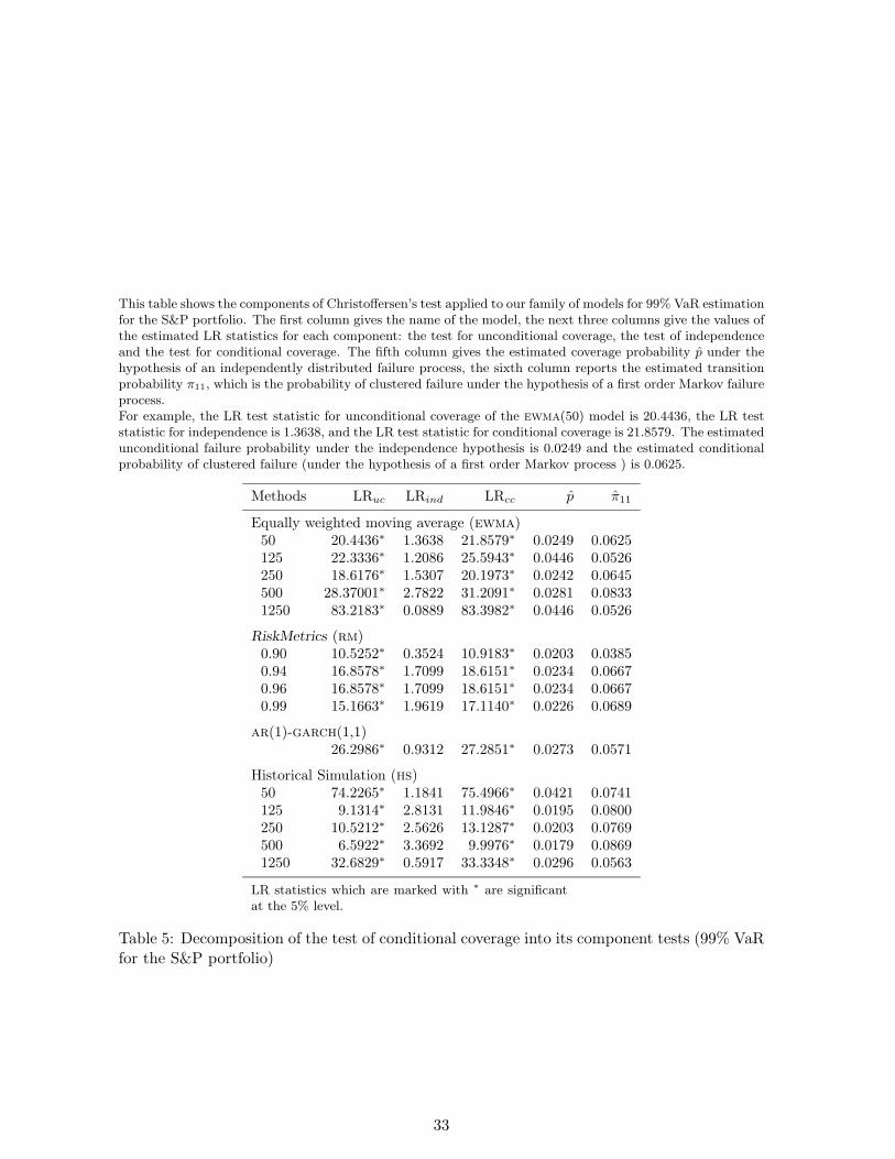
This table shows the components of Christoffersen’s test applied to our family of models for 99% VaR estimationfor the S&P portfolio. The first column gives the name of the model, the next three columns give the values ofthe estimated LR statistics for each component: the test for unconditional coverage, the test of independenceand the test for conditional coverage. The fifth column gives the estimated coverage probability p̂ under thehypothesis of an independently distributed failure process, the sixth column reports the estimated transitionprobability π11, which is the probability of clustered failure under the hypothesis of a first order Markov failureprocess.For example, the LR test statistic for unconditional coverage of the ewma(50) model is 20.4436, the LR teststatistic for independence is 1.3638, and the LR test statistic for conditional coverage is 21.8579. The estimatedunconditional failure probability under the independence hypothesis is 0.0249 and the estimated conditionalprobability of clustered failure (under the hypothesis of a first order Markov process ) is 0.0625.

Methods LRuc LRind LRcc p̂ π̂11

Equally weighted moving average (ewma)50 20.4436∗ 1.3638 21.8579∗ 0.0249 0.0625125 22.3336∗ 1.2086 25.5943∗ 0.0446 0.0526250 18.6176∗ 1.5307 20.1973∗ 0.0242 0.0645500 28.37001∗ 2.7822 31.2091∗ 0.0281 0.08331250 83.2183∗ 0.0889 83.3982∗ 0.0446 0.0526

RiskMetrics (rm)0.90 10.5252∗ 0.3524 10.9183∗ 0.0203 0.03850.94 16.8578∗ 1.7099 18.6151∗ 0.0234 0.06670.96 16.8578∗ 1.7099 18.6151∗ 0.0234 0.06670.99 15.1663∗ 1.9619 17.1140∗ 0.0226 0.0689

ar(1)-garch(1,1)26.2986∗ 0.9312 27.2851∗ 0.0273 0.0571

Historical Simulation (hs)50 74.2265∗ 1.1841 75.4966∗ 0.0421 0.0741125 9.1314∗ 2.8131 11.9846∗ 0.0195 0.0800250 10.5212∗ 2.5626 13.1287∗ 0.0203 0.0769500 6.5922∗ 3.3692 9.9976∗ 0.0179 0.08691250 32.6829∗ 0.5917 33.3348∗ 0.0296 0.0563

LR statistics which are marked with ∗ are significantat the 5% level.

Table 5: Decomposition of the test of conditional coverage into its component tests (99% VaRfor the S&P portfolio)

33

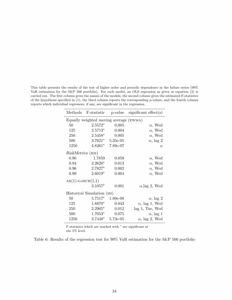
This table presents the results of the test of higher order and periodic dependence in the failure series (99%VaR estimation for the S&P 500 portfolio). For each model, an OLS regression as given in equation (2) iscarried out. The first column gives the names of the models, the second column gives the estimated F-statisticsof the hypothesis specified in (1), the third column reports the corresponding p-values, and the fourth columnreports which individual regressors, if any, are significant in the regression.

Methods F-statistic p-value significant effect(s)

Equally weighted moving average (ewma)50 2.5572∗ 0.005 α, Wed125 2.5713∗ 0.004 α, Wed250 2.5458∗ 0.005 α, Wed500 3.7621∗ 5.35e-05 α, lag 21250 4.8261∗ 7.89e-07 α

RiskMetrics (rm)0.90 1.7859 0.059 α, Wed0.94 2.2620∗ 0.013 α, Wed0.96 2.7827∗ 0.002 α, Wed0.99 2.6019∗ 0.004 α, Wed

ar(1)-garch(1,1)3.1057∗ 0.001 α,lag 2, Wed

Historical Simulation (hs)50 5.7517∗ 1.80e-08 α, lag 2125 1.8870∗ 0.043 α, lag 1, Wed250 2.2905∗ 0.012 lag 1, Tue, Wed500 1.7053∗ 0.075 α, lag 11250 3.7448∗ 5.73e-05 α, lag 2, Wed

F statistics which are marked with ∗ are significant atthe 5% level.

Table 6: Results of the regression test for 99% VaR estimation for the S&P 500 portfolio

34

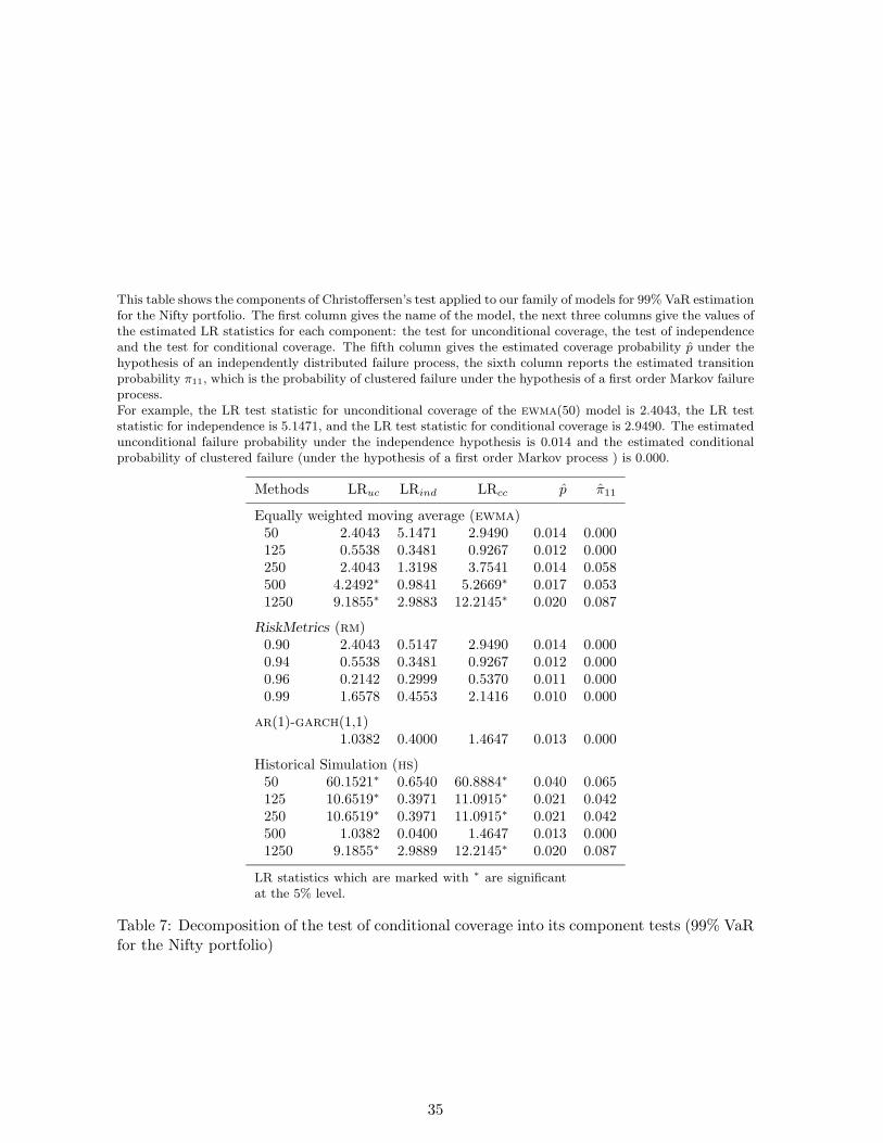
This table shows the components of Christoffersen’s test applied to our family of models for 99% VaR estimationfor the Nifty portfolio. The first column gives the name of the model, the next three columns give the values ofthe estimated LR statistics for each component: the test for unconditional coverage, the test of independenceand the test for conditional coverage. The fifth column gives the estimated coverage probability p̂ under thehypothesis of an independently distributed failure process, the sixth column reports the estimated transitionprobability π11, which is the probability of clustered failure under the hypothesis of a first order Markov failureprocess.For example, the LR test statistic for unconditional coverage of the ewma(50) model is 2.4043, the LR teststatistic for independence is 5.1471, and the LR test statistic for conditional coverage is 2.9490. The estimatedunconditional failure probability under the independence hypothesis is 0.014 and the estimated conditionalprobability of clustered failure (under the hypothesis of a first order Markov process ) is 0.000.

Methods LRuc LRind LRcc p̂ π̂11

Equally weighted moving average (ewma)50 2.4043 5.1471 2.9490 0.014 0.000125 0.5538 0.3481 0.9267 0.012 0.000250 2.4043 1.3198 3.7541 0.014 0.058500 4.2492∗ 0.9841 5.2669∗ 0.017 0.0531250 9.1855∗ 2.9883 12.2145∗ 0.020 0.087

RiskMetrics (rm)0.90 2.4043 0.5147 2.9490 0.014 0.0000.94 0.5538 0.3481 0.9267 0.012 0.0000.96 0.2142 0.2999 0.5370 0.011 0.0000.99 1.6578 0.4553 2.1416 0.010 0.000

ar(1)-garch(1,1)1.0382 0.4000 1.4647 0.013 0.000

Historical Simulation (hs)50 60.1521∗ 0.6540 60.8884∗ 0.040 0.065125 10.6519∗ 0.3971 11.0915∗ 0.021 0.042250 10.6519∗ 0.3971 11.0915∗ 0.021 0.042500 1.0382 0.0400 1.4647 0.013 0.0001250 9.1855∗ 2.9889 12.2145∗ 0.020 0.087

LR statistics which are marked with ∗ are significantat the 5% level.

Table 7: Decomposition of the test of conditional coverage into its component tests (99% VaRfor the Nifty portfolio)

35

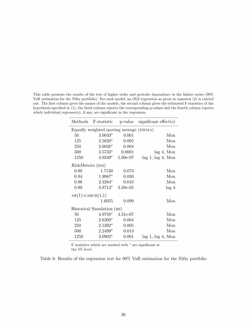
This table presents the results of the test of higher order and periodic dependence in the failure series (99%VaR estimation for the Nifty portfolio). For each model, an OLS regression as given in equation (2) is carriedout. The first column gives the names of the models, the second column gives the estimated F-statistics of thehypothesis specified in (1), the third column reports the corresponding p-values and the fourth column reportswhich individual regressor(s), if any, are significant in the regression.

Methods F-statistic p-value significant effect(s)

Equally weighted moving average (ewma)50 3.0033∗ 0.001 Mon125 2.5620∗ 0.005 Mon250 2.6026∗ 0.004 Mon500 3.5733∗ 0.0001 lag 4, Mon1250 4.9249∗ 5.30e-07 lag 1, lag 4, Mon

RiskMetrics (rm)0.90 1.7130 0.073 Mon0.94 1.9987∗ 0.030 Mon0.96 2.3284∗ 0.010 Mon0.99 3.8713∗ 3.50e-05 lag 4

ar(1)-garch(1,1)1.6055 0.099 Mon

Historical Simulation (hs)50 4.9758∗ 4.31e-07 Mon125 2.6300∗ 0.004 Mon250 2.5392∗ 0.005 Mon500 2.2499∗ 0.013 Mon1250 3.0903∗ 0.001 lag 1, lag 4, Mon

F statistics which are marked with ∗ are significant atthe 5% level.

Table 8: Results of the regression test for 99% VaR estimation for the Nifty portfolio

36

This table provides the summary results of the second stage of the model selection procedure applied to thetwo “acceptably accurate” models chosen in the first stage for 99% VaR estimation for the Nifty portfolio.The first column of the table pertains to the “regulatory loss function” (rlf) and the second column to the“Firm’s loss function” (flf) defined in sections 4.1 and 4.2. Panel A reports the average values of rlf andflf for the two competing models. Panel B provides the values of the standerdised sign statistics as givenin section 4.3.1. SRA denotes the standerdised sign statistic for testing the hypothesis of “non-superiority ofrm(.90) over ar(1)-garch(1,1)” and SAR denotes the standerdised sign statistic for testing “non-superiorityof ar(1)-garch(1,1) over rm(.90)” in terms of the specific loss functions.

rlf flf

Panel A: Averages values

rm(.90) 0.0861 0.2379ar(1)-garch(1,1) 0.0851 0.2362

Panel B: Sign statistics

SRA 33.48 −2.69∗

SAR 33.07 2.93

Sign statistics which is marked with ∗ is significant atthe 5% level.

Table 9: Summary results of the “Loss function” approach applied to the models chosen inthe first stage

37

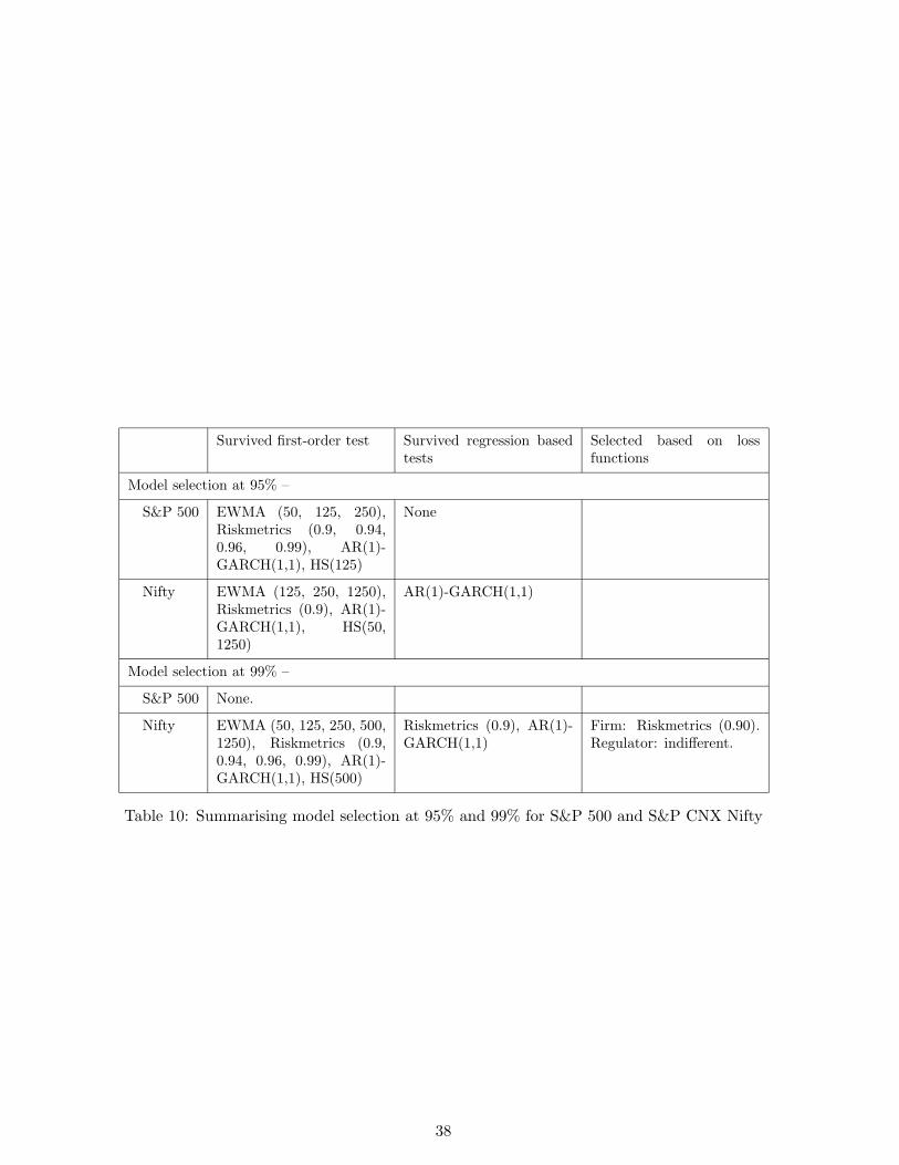
Survived first-order test Survived regression basedtests

Selected based on lossfunctions

Model selection at 95% –

S&P 500 EWMA (50, 125, 250),Riskmetrics (0.9, 0.94,0.96, 0.99), AR(1)-GARCH(1,1), HS(125)

None

Nifty EWMA (125, 250, 1250),Riskmetrics (0.9), AR(1)-GARCH(1,1), HS(50,1250)

AR(1)-GARCH(1,1)

Model selection at 99% –

S&P 500 None.

Nifty EWMA (50, 125, 250, 500,1250), Riskmetrics (0.9,0.94, 0.96, 0.99), AR(1)-GARCH(1,1), HS(500)

Riskmetrics (0.9), AR(1)-GARCH(1,1)

Firm: Riskmetrics (0.90).Regulator: indifferent.

Table 10: Summarising model selection at 95% and 99% for S&P 500 and S&P CNX Nifty

38