ModelOMatic: fast and automated model selection between RY, nucleotide, amino acid, and codon...

1/36

ModelOMatic: fast and automated model selection between

RY, nucleotide, amino acid, and codon substitution models

Simon Whelan1,2, James E. Allen2, Benjamin P. Blackburne2, David Talavera2

1 Evolutionary Biology, Evolutionary Biology Centre, Uppsala University, SE

2 Faculty of Life Sciences, University of Manchester, Manchester, UK

Corresponding author

Simon Whelan

Evolutionary Biology

Evolutionary Biology Centre

Uppsala University

Uppsala 75236

Sweden

Tel: +46-(0)18-4716483

e-mail: [email protected]

Key words

Phylogenetics; substitution models; model selection; AIC;

© The Author(s) 2014. Published by Oxford University Press, on behalf of the Society of Systematic Biologists. All rights reserved. For Permissions, please email: [email protected]

Systematic Biology Advance Access published September 9, 2014 by guest on June 22, 2016

http://sysbio.oxfordjournals.org/D

ownloaded from

by guest on June 22, 2016


ownloaded from



ownloaded from



ownloaded from

http://sysbio.oxfordjournals.org/




2/36

Abstract

Molecular phylogenetics is a powerful tool for inferring both the process

and pattern of evolution from genomic sequence data. Statistical approaches,

such as maximum likelihood and Bayesian inference, are now established as the

preferred methods of inference. The choice of models that a researcher uses for

inference is of critical importance, and there are established methods for model

selection conditioned on a particular type of data, such as nucleotides, amino

acids, or codons. A major limitation of existing model selection approaches is

that they can only compare models acting upon a single type of data. Here we

extend model selection to allow comparisons between models describing

different types of data by introducing the idea of adapter functions, which

project aggregated models onto the originally observed sequence data. These

projections are implemented in the program ModelOMatic and used to

perform model selection on 3,722 families from the PANDIT database, 68 genes

from an arthropod phylogenomic data set, and 248 genes from a vertebrate

phylogenomic data set. For the PANDIT and arthropod data, we find that amino

acid models are selected for the overwhelming majority of alignments; with

progressively smaller numbers of alignments selecting codon and nucleotide

models, and no families selecting RY-based models. In contrast, nearly all

alignments from the vertebrate data set select codon-based models. The

sequence divergence, the number of sequences, and the degree of selection

acting upon the protein sequences may contribute to explaining this variation in

model selection. Our ModelOMatic program is fast, with most families from

PANDIT taking fewer than 150 seconds to complete, and should therefore be

easily incorporated into existing phylogenetic pipelines.

by guest on June 22, 2016http://sysbio.oxfordjournals.org/

Dow

nloaded from


3/36

Introduction

The comparison of molecular sequence data in phylogenetics is a

statistical problem (Felsenstein 2003; Yang 2006). Modern approaches to the

problem use probabilistic substitution models, which describe biological factors

affecting molecular evolution through parameterisations of the relative rates of

substitution between the characters in a sequence (Yang and Rannala 2012). The

parameters of these models are inferred using statistical inference methods,

such as maximum likelihood or Bayesian inference (Kosiol, et al. 2006; Yang

2006). These inferential methods are statistically consistent, meaning that as

data are added they asymptotically tend towards the correct answer, providing

an adequate substitution model is used (Rogers 1997). There has been a

substantial research effort to create more realistic substitution models of protein

evolution that capture a wide range of evolutionary pressures, including generic

evolutionary pressures (Le and Gascuel 2008; Whelan and Goldman 2001), the

pressures resulting from protein structure (Liberles, et al. 2012; Thorne, et al.

1996), and selective pressures specific to individual sites (Halpern and Bruno

1998; Lartillot and Philippe 2004).

The importance of substitution models has led to model selection

becoming standard practice in phylogenetic studies. Model selection typically

follows an information-theoretic approach where a score, such as the Akaike

Information Criteria or the Bayesian Information Criteria, is used to measure the

fit of a model to a specific data set (Burnham and Anderson 2002; Posada and

Buckley 2004; Sullivan and Joyce 2005). These approaches are implemented in

the widely used jModelTest (Darriba, et al. 2012; Posada 2008) and ProtTest

(Darriba, et al. 2011) programs. Information-theoretic model selection measures

the relative fit of a set of models to the observed data, but does not assess

whether they those data are likely to have arisen under that model. Several

studies have suggested that model adequacy should be assessed alongside model

selection (Bollback 2002; Goldman 1993) or that model selection could be

conducted based on the performance of those models in estimating the

parameters of interest (Brown 2014; Minin, et al. 2003). Both assessment of


Dow

nloaded from


4/36

model adequacy and performance-based model selection, although not widely

used, provide valuable alternative perspectives to the information-theoretic

approach.

All model selection methods are dependent on the type of data analysed.

Models of amino acid substitution, for example, cannot be directly compared to

models of nucleotide substitution because they exist in different state-spaces.

More formally, the likelihood function is conditioned upon the state-space of the

model (Burnham and Anderson 2002), meaning that likelihoods obtained under

4-state nucleotide substitution models cannot be compared to likelihoods

obtained under 20-state amino acid substitution models. The inability to

compare likelihoods means we cannot use any standard approaches for model

selection across state-spaces, with the problem affecting both maximum

likelihood and Bayesian inference because both link observed data to the

substitution model through the same likelihood function (Yang 2006).

This limitation has resulted in a dearth of research on the comparison and

selection of substitution models between state-spaces. Most studies dealing with

model selection do not consider the possibility of choosing between state-spaces,

instead concentrating on model selection in one state-space, such as quantifying

the performance of model selection on nucleotide sequences with maximum

likelihood (Posada and Crandall 2001) and Bayesian inference (Huelsenbeck, et

al. 2004), or investigating the fit of amino acid substitution models (Keane, et al.

2006). Some studies have attempted to use simulation or properties of real data

to understand the relationship and performance between different state-spaces,

with most methods applying these approaches to models of RNA dinucleotide

evolution (Gibson, et al. 2005; Letsch and Kjer 2011; Schöniger and von Haeseler

1999; Telford, et al. 2005). An important exception to this pattern is a small

number of pioneering works that attempted to describe the statistical

relationships between state-spaces. These works include aggregating models

from larger state-spaces to smaller state-spaces, such as from codons to amino

acids (Yang, et al. 1998), and projecting models from smaller state-spaces to


Dow

nloaded from


5/36

larger state-spaces, such as the projection of nucleotide models or amino acid

models to codon models (Seo and Kishino 2009, 2008; Whelan and Goldman

2004) or the projection of 7-state RNA models to 16-state RNA models (Allen

and Whelan 2014).

This study takes a different approach for model comparison across state-

spaces by incorporating the aggregation step, where the originally observed

sequences are compressed to a lower state-space, into substitution models. Our

starting rationale is that all models used to analyse an alignment of sequences

must be capable of generating those sequences in their original state-space. In

other words, all models should be conditioned on the original sequence data and

not on their own aggregated forms of those data. We address this problem by

developing adapter functions that project the output of models from the

aggregated state-space onto the state-space of the original sequence. The

outcome of this approach is a generalised ‘correction’ that allows the comparison

of likelihoods obtained from models under any aggregated state-space, providing

they originated from the same original sequences. This approach is also used to

accommodate the comparison of mixture models across state-spaces, such as the

comparison of a nucleotide substitution model with Γ-distributed rates-across-

sites to a codon model. To demonstrate the utility of our approach, we develop a

model selection approach for choosing the best-fit model to describe protein-

coding regions, allowing a wide range of models from many different state-

spaces to be compared. These models and their corresponding projections are

implemented in a new program called ModelOMatic, which can rapidly select

the best model and state-space for performing phylogenetic analysis based on

information-theoretic measures. We apply this program to large numbers of

families from the PANDIT database (Whelan, et al. 2003; Whelan, et al. 2006) and

two phylogenomic data sets from arthropods (Regier, et al. 2010) and

vertebrates (Chiari, et al. 2012) to demonstrate its utility and to investigate

factors affecting model choice. For PANDIT and the arthropod data set, we find

the overwhelming majority of alignments select a version of the LG amino acid

substitution model (Le and Gascuel 2008) with Γ-distributed rates across sites.


Dow

nloaded from


6/36

For the vertebrate data set, nearly all alignments select models from the codon

state-space.

Materials and methods

Substitution models

Here we describe general principles of how substitution models

describing sequence evolution can be compared between state-spaces. First we

define models and sequences in our original and aggregated state-space. We

proceed to define the reverse of the aggregation step as a probabilistic process,

which allows substitution models acting on the aggregated sequences to be fitted

on the original sequences. This approach can be used to create a general

likelihood ‘correction’ that accounts for differences between state-spaces,

leading to a simple and fast method for model comparison between state-spaces.

Definitions

A phylogenetic substitution model is usually described through the

instantaneous rate matrix of a Markov process, �, which describes the rate of

change between two discrete characters �� and�� . We define a Distinct Model by

the instantaneous rate matrix ��, which describes the rates of change between

characters in the Distinct Model state-space, � = {�, … , � }. The state-space of

the Distinct Model is considered to be the original or natural state-space from

which the observed sequences were generated. A Compound Model, defined by

��, is one that is formed by aggregating �� such that a set of states in �

correspond to a single state in the Compound Model state-space, � = {�, … , ��}. Each state in D maps to a single state in C, so the relationship between the state-

spaces can be expressed through an explicit mapping function such that ��(�) links the distinct state �� with the compound state ��, and the reverse mapping

whereby the set of � distinct states contained within the compound state is

expressed as ��̅ = {�(�), … , ��(�)}. For clarity and brevity, substitutions

between states in � are indexed � and �, whereas substitutions between states in

�are indexed � and �. An aligned set of sequences from � and � are referred to


Dow

nloaded from


7/36

as �� and ��, respectively. Following standard notation, the substitution process

of the Compound Model can be parameterised such that ��,�� = ��,�� ∀� ≠ �, where ��,�� corresponds to the ‘exchangeability’ parameter between characters �� and

�� , and �� the equilibrium frequency of state �� (Whelan, et al. 2001; Yang

2006). The equilibrium frequencies of the Distinct Model are defined as

#$(�)� = ��, where the right hand side provides a convenient shorthand. The

totality of parameters from the Compound Model and Distinct Model can be

expressed as %� and %�, respectively. Over time & the probability matrices for

transitions between the characters from � and � are expressed as '�(&) and

'�(&), respectively.

Projecting a single Compound Model onto a Distinct Model state-space

The likelihoods of models with different state-spaces cannot usually be

compared because they are conditioned upon different data. In molecular

phylogenetics, however, we have a special scenario, where our initial

observation is of a set of protein-coding genomic sequences, but it may be

convenient to analyse them using a range of aggregated state-spaces, either due

to practical reasons, such as computational tractability, or scientific reasons,

whereby raw nucleotides do not capture the interdependencies between

characters induced by the genetic code (Whelan 2008). This choice between

direct modelling and aggregation is illustrated in Figure 1, where the original

genomic sequences are in the codon state-space and can be analysed in either

the original (codon; Distinct Model) state-space or the aggregated (amino acid;

Compound Model) state-space. The likelihood from the codon model,

((��)*)+|%�)*)+), and the likelihood from the amino acid model, ((�--|%--) are

not comparable because they are conditioned on different data. A similar

situation occurs when trying to compare likelihoods from models describing

other aggregated state-spaces, such as nucleotides or RY.

To address this problem we propose adding an additional term to the

Compound Model likelihood called an adapter function, P(��|��). This function


Dow

nloaded from


8/36

effectively provides a modelling component that reverses the aggregation step

used to produce � from �, allowing each known state in C to be ‘projected’ onto

the set of possible states in � from which it could have come. The adapter

function is applied after the Compound Model has generated sequences in � and

therefore contains no information about the phylogenetic tree. The practical

outcome of adding this adapter function to a Compound Model is that it now

generates sequences in �, allowing the likelihood of the original (Distinct Model)

state-space to be written in terms of the Compound Model likelihood and the

adapter function:

((��; %�) = ((��; %�)P(��|��) (2)

There are several key decisions when trying to create this adapter

function, which we will summarise here, although full details are available in the

Appendix. We propose the simplest form of adapter function possible, which

takes a state �� and projects it to one of the corresponding Distinct Model state,

��(�) ∈ ��̅, with probability P(�(�)|��) = #1(�)� /∑ #$(�)�#$∈45̅ = #1(�)� / ��. This

adapter function term is independent of the likelihood function of the Compound

Model, acts on each character in the data independently, and introduces up to a

maximum of |�| − |�| free parameters to the model. This approach means the

adapter function can be written in terms of which characters occur in �� and ��

and the frequency with which they occur:

((��; %�) = ((��; %�)∏ ∏ 89(:,;)<

8=(:,;)>LengthETaxaI (3)

where �(J, K) and �(J, K) are the character states in the original data matrix

from the Jth taxa and Kth site for the multiple sequence alignments recoded to

the � and �, respectively. For example, if character �(J, K) is the codon TGG, then

under an amino acid state-space the corresponding character �(J, K) would be

tryptophan (W). In practice, the term P(��|��) works as a ‘correction’ for the


Dow

nloaded from


9/36

likelihood function, adjusting it to explicitly state that the sequences observed in

�� are an aggregation of those observed in ��. This projection is illustrated in

Figure 1 where the ‘greyed out’ amino acid sequences can be considered an

intermediary step when calculating (L��)*)+; %--M. This projected Compound

Model likelihood, ((��; %�), can now be compared directly to the Distinct Model

likelihood, ((��; %�), because they are conditioned on the state-space of the

original sequence. Moreover, the likelihood from a range of different Compound

Models can be compared providing they are all conditioned on the same original

sequence state-space.

Projecting mixtures of Compound Models onto a single Distinct Model state-space

The approach described above provides a simple way to project the

output of the Compound Model onto the Distinct Model state-space given an

observed sequence. This approach is suitable for comparing simple substitution

models, but we may want to compare mixtures of Compound Models to models

from the Distinct Model state-space. This type of problem takes two forms and

detailed explanations of our approaches to enable model comparison under

these conditions are provided in the Appendix.

The first approach we examine projects random-effects mixtures of N

Compound Models – where the evolution of each site in an alignment is assigned

some form of substitution process, %�(O), according to a probability distribution –

to the Distinct Model state-space. An example of this type of comparison occurs

when we wish to compare an amino acid (Compound) model with Γ-distributed

rates-across-sites to a codon (Distinct) model. In order to perform this projection

we need to consider each mixture component of the Compound Model

substitution process in turn (e.g. each individual rate category from a Γ-

distribution) and provide an adapter function for it. This approach means that

we can apply equation (3) to each of the mixture categories in turn and compute

their likelihood before mixing them back together.


Dow

nloaded from


10/36

((��; %�) = ∑ P(%�(O))((��; %�(O))P(��|��(O))O (4)

However, if we assume that �� is the same across the mixture components, then

the adapter function and the Compound Model likelihood are independent,

which means that they can be separated from one another. Under these

conditions the same adapter function is applied to all mixtures and we find that

we can separate ((��; %�) into the ‘correction’ term provided by the projection

and the likelihood of the mixture of Compound Models:

((��; %�) = Q∏ ∏ 89(:,;)<

8=(:,;)>LengthETaxaI R∑ P(%�(O))((��; %�(O))O (5)

A similar approach can be taken for the second type of mixture model,

where the Distinct Model state-space is made of multiple instances of the

Compound Model state-space. For example, the codon (Distinct Model) state-

space of a codon is made from three individual instances of the nucleotide

(Compound Model) state-space. In these cases, the Distinct Model state-space

can be described by a sequential set of Compound Models, where %�(S) is the

model at the TUV position. Again we assume �� is the same across the mixture

components. In this case we can treat each of the Compound Models as an axis in

a multidimensional stochastic process that generates sequence in the Distinct

Model state-space. The individual Compound Models do not interact, so the

likelihood of the set of Compound Models is the product of their likelihoods:

((��; %�) = ∏ (L��(S); %�(S)M�(S)∈� (6)

These two cases represent the majority of applications of mixture models used in

phylogenetics and are adequate for providing projections onto most commonly

used state-spaces. It is also trivial to generalise our approach to cases where ��

varies between mixture components.


Dow

nloaded from


11/36

Parameterisation of the likelihood correction function

The correction described by equations (3) and (5) requires knowledge of

the equilibrium frequencies of the Distinct Model in order to calculate the

projected likelihood for the Compound Model. These frequencies should be

represented as free parameters in the Compound Model and their presence

needs to be accounted for in model comparison (see below). We investigate two

parameterisations of #$(�)� in the compound model, which represent the two

extremes of complexity in all possible parameterisations. The first ‘EQUAL’

approach is the lowest complexity and assumes only knowledge of the

frequencies of the Compound Model, so that #$(�)� = �� |��̅|⁄ . This

parameterisation adds no degrees of freedom to the model. The second ‘EMP’

approach represents the most complex scenario, which is to treat the #$(�)�

parameters as free parameters in the model. One can compute a standard

likelihood function for the EMP projection, but for the purpose of model

comparison we only need the ML estimates (MLEs), which are exactly expressed

as the empirical frequencies of the distinct characters in the data, X#$(�)� , scaled

so they reflect the frequencies from the compound model: #$(�)� = X#$(�)� �� X��Y ,

where X�� is the empirical compound state frequency. From this formulation it is

evident that using MLEs in the EMP projection adds |�| − |�| degrees of freedom

to the Compound Model.

Comparison to the Seo and Kishino approach

Conceptually there are similarities between our approach and that of Seo

and Kishino (2008; hereafter referred to as SK08), but the comparison between

our projection method and SK08 also provides some insight into the similarities

and differences between models in different state-spaces. The general SK08

approach reverses the aggregation step in the substitution model by building a

codon substitution model from the parameters of the amino acid substitution

model. (See Figure 1 for an illustration.) This approach is valid for creating

comparable models, but runs into problems regarding its generality. The codon


Dow

nloaded from


12/36

model produced by SK08 is only one of many possible codon models that would

exactly match the amino acid model when aggregated. Seo and Kishino (2008)

explore a small subspace of these codon models by parameterising SK08 with Z,

but their approach does not provide complete generality since they do not show

that the resulting codon models provide better fits than the set of all possible

codon models that aggregate to the original amino acid model.

In contrast, our approach reverses the aggregation step at the sequence

level. This allows us to use an exact representation of the Compound Model,

encompassing all of its properties, and then project its output onto the Distinct

Model state-space. This projection is achieved through a simple adapter function

that allows the Compound Model to describe substitutions in its own state-space,

but give rise to sequences in the Distinct Model state-space. In common with

SK08 model projection, the sequence projection given by our adapter function is

not unique. However, we suggest that the EQUAL and EMP parameterisations

provide a reasonable summary of the different possible parameterisations and

are suitable for most model selection applications.

Given these fundamental differences in approach it is intriguing to

observe that our likelihood correction in equation (3) is identical to equation (6)

from Seo and Kishino (2008). In SK08, equation (6) is obtained by setting the

rate of substitution between all characters in � that are not directly observable

in �, to infinity; in other words �#$(�),#[(�)� = ∞. We provide a brief summary

explaining why the process generating sequences from this Distinct Model with

infinite rates is exactly equivalent to generating sequences from the Compound

Model and projecting it to the Distinct Model state-space. Under the Distinct

Model the likelihood of observing the character � given a root character of � is

simply an element from the '�(&) matrix. Following Chapman-Kolmogorov we

can write:

]#$(�),#[(�)� (& + _) = ∑ ]#$(�),#`(O)� (&)]#`(O),#[(�)� (_)#`(O)


Dow

nloaded from


13/36

The infinite rate between �#$(�),#[(�)� means that our ability to discriminate

between the specific value of ��(�) and the elements of ��̅ disappears as the

process instantaneously reaches equilibrium, meaning that the first term of the

right hand side can be written solely in terms of the Compound Model. As _ tends

to zero, the second term is equivalent to our projection function P(��(�)|�), leading to:

]#$(�),#[(�)� (&) = ]�,�� (&)P(��(�)|��̅)

which when incorporated into the likelihood function for a set of sequences

leads to our equation (3) and equation (6) from Seo and Kishinos (2008). (Full

details of this proof are provided in the Appendix.)

Substitution models examined

In total 152 substitution models are compared for each multiple sequence

alignment examined. These can be conceptually grounded in 38 foundation

models, which can be subdivided by the state-space they examine and the

exchangeability and frequency parameters they define (see Table 1). The pair of

binary choices of whether models use Γ-distributed rates-across-sites or not

(four discrete categories; Yang 1994), and whether they use EQUAL or EMP

frequencies in the adapter function provide four additional options for each of

the foundation models (38 foundation models x {EQUAL⨁EMP} x {–Γ⨁+Γ} = 152

substitution models).

Model selection

For formal model selection we use the Akaike Information Criterion (AIC:

Akaike 1974). We note it is possible to use the corrected version of AIC with the

approximation of sample size of Posada and Buckley (2004) or BIC, although our

exploratory data analysis finds the choice of information theoretic measure has


Dow

nloaded from


14/36

minimal effect on model selection for our sequence data. For coding sequences it

is appropriate to select models based on their AIC on a 64 character state-space

corresponding to the Distinct Model describing all possible nucleotide triplets,

including coding and stop codons. For each model we calculate its maximal log-

likelihood under the Distinct Model state-space under both the EQUAL and EMP

corrections, then calculate an AIC value using an appropriate number of degrees

of freedom. Following standard theory the smallest AIC corresponds to the best-

fitting model (Burnham and Anderson 2002). The fit of other models is assessed

through the ΔAIC statistic, which measures the difference between their AIC and

that of the best-fit model. Smaller values of ΔAIC reflect models closer to the

best-fit model.

Sequence data and implementation

The first set of sequence data examined is taken from the PANDIT

database (version 17.0; Whelan, et al. 2003; Whelan, et al. 2006). We filter the

families available in PANDIT according to the following criteria: (i) there must be

between 6-100 sequences; (ii) the alignment must be >= 50 codons in length;

(iii) all branches of the DNA PANDIT tree and AA PANDIT tree must be <0.5 in

their respective time units; (iv) the coding sequence is compatible with the

universal genetic code; and (v) no sequence may have >85% gap characters in

any one sequence at the amino acid level. A small number of families were also

rejected due to errors during computation. These filters yielded 3 722 PANDIT

families available for further study, with a mean of 18.6 (interquartile range: 8,

21) sequences of length 707.9 nucleotides (327, 921) per family. We also

examine two phylogenomic data sets taken from the recent literature: (i) 68

arthropod protein-coding genes from Regier, et al. (2010), where each gene

covers an average of 64.9 taxa from a maximum of 80; and (ii) 248 vertebrate

protein-coding genes from (Chiari, et al. 2012), where each gene covers an

average of 11.4 taxa from a maximum of 16 taxa.


Dow

nloaded from


15/36

All computation and model comparison is performed in the C++

ModelOMatic program, available through a GNU GPL v3 license at the

googlecode repository: https://code.google.com/p/modelomatic/. The program

takes as input a multiple sequence alignment in sequential or interleaved format.

There is also an option to provide a Newick formatted tree or have the program

estimate one using the BIONJ algorithm from a Poisson amino acid substitution

model (Yang 2007) with empirically estimated amino acid frequencies ('+F'; see

Goldman and Whelan 2002). Extensive comparisons between results obtained

under the BIONJ tree with those obtained using the phyml (Guindon and

Gascuel 2003) derived ‘amino acid’ tree provided in PANDIT (Whelan, et al.

2003; Whelan, et al. 2006) suggest tree topology has a limited affect on model

selection. In total 3,499/3,715 (94.2%) of families showed no difference in the

best-fit model between the two topologies. Moreover, for 165 out of the 216

families showing differences, the best-fit model is from the same state-space. A

second consideration when estimating MLEs is the degree of rigour with which

the parameters are optimised. During the development of ModelOMatic we

considered full (slow; high rigour) optimisation and heuristic approximations

(fast; lower rigour). The results presented here are from our fast version of the

program, but results are very similar for the full version. For the PANDIT

database analysis, we find in 3,385/3,719 (91.0%) of families there is agreement

between the best-fit model under full and fast versions, and that our heuristics

make no change to the selected best-fit state-space in 3,651/3,719 (98.2%) of

families. (Note that the total number of families used in these performance

comparisons vary due to program failures when using particular heuristics and

that the exact details of the nodes used to run the program vary, with processor

speeds ranging between 2.27GHz-2.67GHz and memory ranging between 24Gb-

504Gb.)

Results

Finding optimal model fit in PANDIT protein domains

To assess the relative fit of RY, nucleotide, amino acid, and codon models,

the fast version of ModelOMatic was run on the 3,722 PANDIT families. Table 2


Dow

nloaded from


16/36

shows how frequently different state-spaces and specific models were chosen as

the best-fit model according to AIC. The large majority of families (3,363/3,722)

lead to a model describing amino acid substitutions to be selected, followed by

some families selecting a codon model (349/3,722), and a small number

(10/3,722) selecting a nucleotide model. No families found the RY state-space to

provide the best-fit model substitution model. Furthermore, in the

overwhelming majority of families (3,632/3,722) the Γ-distributed rates-across-

sites version of models provides a better fit than the equal rates-across-sites

version.

There is substantial variation in the model chosen for each state-space,

albeit with a tendency towards more complex models. For the nucleotide state-

space only HKY+Γ or REV+Γ were chosen, suggesting evidence of substantial

variation in the rates of substitution between nucleotides. For the amino acid

state-space no single model was consistently chosen. The most frequently

chosen baseline model was LG, which was selected in 2,412 (64.9%) of families,

with an even split between ‘-F’ and ‘+F’ amino acid frequencies of 1,265 and

1,147, respectively. The strong preference for LG could be expected since the LG

model was trained on a superset of families from Pfam (Finn, et al. 2010), upon

which PANDIT is based. The WAG, VT, rtREV, and JTT models were all selected in

over 100 families, whereas other amino acid substitution models were selected

much less frequently. These other models include those trained on other genetic

codes and genes held on organelle genomes, which might be expected to be

subjected to different selective pressures from ‘regular’ nuclear genes. For the

codon state-space all four possible descriptions of codon frequencies were

chosen, but the majority of families (212/349) that selected the codon state-

space also selected an individual frequency for each codon (F64). The total

number of families selecting each codon model corresponds with the complexity

of the model, such that the more complex the model, the more likely it is to be

chosen.


Dow

nloaded from


17/36

Relative model fit for different state-spaces

Compiling the list of best-fit models provides only a superficial insight

into how well different models in different state-spaces describe the data. A

model or state-space could have a very competitive AIC for all families, but rarely

be the best-fit for any individual family, suggesting a robust performance of the

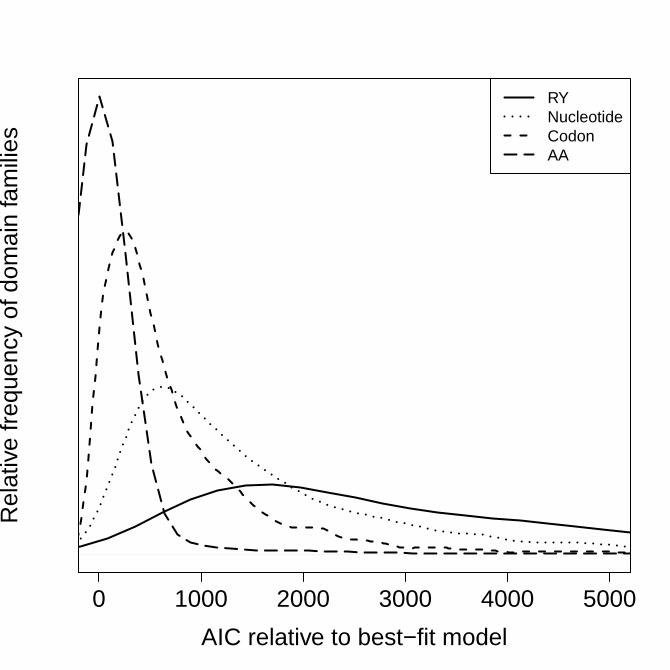
state-space. Figure 2 shows how the best-fit models from each state-space

compare to one another. Given the frequency that amino acid models are

selected as the best-fit model, the observation that the best-fitting state-space

tends to be that of amino acids is to be expected. Figure 2 shows there is,

however, a substantial difference in AIC between amino acids and other state-

spaces, with median (upper-; lower-quartile ranges) ΔAIC values of 477.3 (213.1;

987.2) for codons, 1,164.8 (620.1; 2,161.8) for nucleotides, and 2,983.5 (1,653.8;

5,734.1) for RY recoding. These ΔAIC values are large and suggest that models

describing substitutions in the amino acid state-space capture evolution better

than those of the other state-spaces.

One possible explanation for the dominance of the amino acid state-space

is that the number of possible amino acid models is so large relative to the

number of other models (Table 1). However, at least three factors suggest this is

not the case. First, the majority of amino acid best-fit models are dominated by a

small number of models. The LG+Γ and LG+F+Γ models account for the best-fit

model in 64.6% (2,404/3,722) families, whereas if WAG+F and WAG+F+Γ are

included this rises to 74.4% (2,768/3,722) of families. Second, the gap between

the best-fit amino acid model and the best-fit model of another state-space is

typically very large, suggesting relatively large variations in the amino acid

model may be tolerated before another state-space is selected. Finally, there is a

tendency for sets of amino acid models to be selected ahead of other state-

spaces. In 99.7% (3,354/3,363) of families where an amino acid model is

selected, the second choice model is also an amino acid model. Similarly in

families where an amino acid model is selected, a high proportion of other amino

acid models are selected before another state-space is selected. Around two

thirds of amino acid models are selected before any model of another state-space


Dow

nloaded from


18/36

is selected in around two thirds of families examined. We also note that these

sets of amino acid models also include those trained on different genetic codes

and organisms with very different life histories, such as HIV.

Factors affecting model selection and state-space selection

It is of interest to know which factors affect model selection and state-

space selection when performing phylogenetic inference. The relative dominance

of amino acid substitution models makes it difficult to resolve a clear

relationship, but Figure 3 provides evidence of some trends. Families that select

nucleotide models tend to have a low total divergence (tree length), whereas

families that select codon models tend to have intermediate tree lengths. For all

divergence levels, however, the majority of families select amino acid models. In

Figure 3, for example, the left-hand-tail of the density function is very shallow,

but the total number of families it encompasses is so large so as to dominate the

other data types. We also examined other potential relationships between the

selected state-space and properties of the sequence data. We find that neither

the number of sequences in an alignment nor the number of sites in an alignment

is predictive of the model or state-space chosen. Note, however, that the lengths

of protein domain alignments tend to be relatively similar, so examining a

greater range of alignments lengths may reveal a predictive relationship.

The strength and form of the selective pressures acting upon the coding

sequences could also influence the model selected. Neutrally or nearly neutrally

evolving proteins, with dN/dS values close to 1.0, could be more difficult to

differentiate from DNA sequences, whereas strong selection may result in very

different patterns of evolution. We find that the dN/dS rate ratios vary

substantially between the sets of state-spaces for the models selected. DNA

models tend to be selected for protein families with lower levels of purifying

selection, with the median dN/dS value along the sequence equal to 0.8 (range

0.3 – 1.9), whereas codon models tend to be selected for families with a median

dN/dS of 0.2 (range 0.1 – 2.0), indicating moderate purifying selection. Amino


Dow

nloaded from


19/36

acid models tend to be selected for families with stronger purifying selection,

with a median dN/dS of 0.1 (range 0.1 – 0.5).

Computation time

Another important consideration in model selection procedures is the

amount of computation time required. Figure 4 shows the overall computation

time required to run ModelOMatic and select both the best-fit model and state-

space. On average the program takes 78.0 seconds to complete (interquartile

range: 45.2 to 147.4 seconds), although a small number of families take

considerably longer (maximum 1,545.0 seconds). Figure 4 also shows a

breakdown of how long different components of the model selection process

take to complete. The RY and nucleotide model selection components are

extremely fast, taking 0.9 seconds (interquartile range 0.3 to 3.5 seconds) and

5.3 seconds (2.8 to 10.0 seconds), respectively. The amino acid model selection

component is a little slower, taking on average 27.8 seconds to complete (15.4 to

51.6), reflecting the larger number of models compared and the increased size of

the state-space. The codon model selection is slower still and the most

computationally intensive component of the model selection process, taking on

average 43.3 seconds to complete (25.5 to 81.8), including a small number of

families that take over 800 seconds to complete. This computation time also

reflects the substantially larger state-space and the need to estimate more model

parameters from the data.

Model selection in phylogenomic data sets

In order to study the generality of the results obtained from PANDIT we

also investigate model selection across state-spaces in phylogenomic data sets

covering arthropods (Regier, et al. 2010)and vertebrates (Chiari, et al. 2012).

The results from both data sets are shown in Table 2. The more taxon rich data

set of arthropod genes closely follows the pattern observed for PANDIT: in

65/68 genes an amino acid model is selected and for the majority of these

(54/65) that model is LG. In contrast to the PANDIT domains, the majority of the

arthropod genes selecting an amino acid model also select the “-F” version of that

http://mc.manuscriptcentral.com/systbiol


Dow

nloaded from


20/36

model (58/65), suggesting that the amino acid frequencies of those genes are

relatively close to the amino acid models examined. The remaining 3 genes select

an F64 codon model, which is the most frequent codon model selected by

PANDIT families. A Γ-distributed rates-across-sites model is also selected for all

genes.

Model selection on the vertebrate data follows a different pattern, with

codon models selected for the overwhelming majority of genes (247/248). The

distribution of selected codon models closely follows the pattern observed in

PANDIT, with genes selecting F64 most frequently (126/247) and progressively

fewer genes selecting further simplifications of the model. The single remaining

gene selects the VT-F amino acid model, which was rarely selected for PANDIT

and not selected for the arthropod genes. In general the best-fit model from the

amino acid state-space for these genes shows a different pattern to the

arthropod and PANDIT data sets. In total 38 (15.3%) genes select an amino acid

model based on a different genetic code or organism, such as an HIV-based

model, a mitochondrial model, or a chloroplast model. Moreover, only 28

(11.2%) genes select the LG model, which was selected by the overwhelming

majority of alignments in the other data sets. The overall amount of amino acid

substitution in the vertebrate genes is also lower than the other two data sets.

On average there are only 1.1 expected amino acid substitutions per site for the

vertebrate genes, in contrast to 9.6 for the arthropod data and 17.7 for the

PANDIT data. The single gene where an amino acid state-space is selected has a

tree length of 7.6 amino acid substitutions per site, which is the fifth longest

amino acid tree length observed in those data. The majority of genes again select

a model with Γ-distributed rates-across-sites (208/248), although this is a

smaller fraction than the other two data sets.

Discussion

In this study we have developed a novel and general method for

comparing phylogenetic substitution models across state-spaces and used it to


Dow

nloaded from


21/36

propose a general model selection strategy for protein-coding genes. Previous

attempts to achieve this goal have been limited by the inherent difficulties when

comparing models from different state-spaces. Under standard conditions,

models using different state-spaces are not comparable because they are

conditioned on different data. This difference is clear when one considers what

happens when those models are used to simulate data. Nucleotide substitution

models generate nucleotide sequences and amino acid substitution models

generate amino acid sequences, so there is no intersection in the space of

sequences they output and they cannot, therefore, be compared.

Previous research on reconciling models from different state-spaces has

focussed on trying to create models in one state-space that are analogous to

another in one of two ways. The first works by aggregating the larger state-space

to the smaller state-space, for example by aggregating codon models to amino

acid models (Yang, et al. 1998). If done at the level of the substitution model, this

approach loses information about the larger state-space, whereas simply

aggregating the sequences can disrupt the underlying assumptions of the model

(Kosiol and Goldman 2011). The second approach takes the smaller state-space

model and creates an analogous larger state-space model. For example, a

nucleotide model (Whelan and Goldman 2004) or amino acid model (Seo and

Kishino 2008) can be used to create an analogous codon model. These analogues

can generate sequence data that is comparable to the larger state-space model,

so their likelihoods are comparable. The problem arises because the analogous

model is only one of many possible larger state-space models that could have

been created from the smaller state-space model. This means for valid model

comparison one would have to be able to choose from the unknown, and

potentially very large, set of all possible analogous models.

Our approach is conceptually quite different from previous

reconciliations between state-spaces. We recognise that all of our substitution

models are attempting to describe the set of sequences we observe prior to any

aggregation process. If we wish to transform the state-space of this original


Dow

nloaded from


22/36

sequence to a smaller, more convenient, state-space then the substitution model

we use should explicitly include the aggregation step. This idea is clearer when

thinking about simulating data from our models. Imagine we have an original set

of codon sequences and we wish to compare them to the simulated output from

an amino acid substitution model. We argue that the amino acid substitution

model is incorrectly specified unless it explicitly contains the projection step that

maps amino acids onto codons, because otherwise it could never have generated

the original sequence data. Once this step is included, then the amino acid model

is naturally conditioned on the original sequences and comparable to all other

models also conditioned upon those sequences. To achieve this aim we introduce

simple adapter functions to the likelihood function that project the smaller state-

space model onto the larger state-space model after the substitution process has

finished. In practice, this projection approach can be used to create a ‘correction’

function for the likelihood of the smaller state-space substitution model that

accounts for the aggregation step. The projections we use are not unique, but

take a very simple form, which means the two extremities we examine in the

EQUAL and EMP forms of correction provide a reasonable summary of all

possible projections.

Our adapter functions for correcting likelihoods between state-spaces

have been implemented in the model selection tool ModelOMatic, which allows

users to choose both the best-fit model and the best-fit state-space under which

to analyse their sequence data. To demonstrate the utility of this new tool we

have applied it to selected families from the PANDIT database (Whelan, et al.

2003; Whelan, et al. 2006) and two phylogenomic data sets (Chiari, et al. 2012;

Regier, et al. 2010). For the PANDIT and the arthropod phylogenomic data set,

we find that in the majority of alignments ModelOMatic selects models from

the amino acid state-space rather than models from the other state-spaces

examined. Describing sequence evolution in the codon state-space provided a

better fit to the data in a substantial minority of families for both these data sets.

For the vertebrate phylogenomic data set we find that ModelOMatic selected

codon models for all but one gene. Across all data sets very few genes (or none)


Dow

nloaded from


23/36

were best described by the nucleotide (RY) state-space. These observations

suggest that, in some cases at least, researchers should consider using newly

developed tools for estimating trees using codon models, such as CodonPhyML

(Gil, et al. 2013), because they better describe the evolution of the sequences

than RY, nucleotide, or amino acid models.

The strong performance of models in the amino acid state-space in two

data sets is somewhat unexpected. Models from the RY, nucleotide, and codon

state-spaces all have more flexibility in how they describe relative rates due to

their parameterisations, whereas amino acid models provide fixed empirically

derived estimates of the relative rates of substitution. Moreover, other research

has suggested that amino acid models represent an aggregated process, meaning

that the process the models are trying to describe is non-Markovian (Kosiol and

Goldman 2011). Our examination of the factors affecting model choice on the

PANDIT data set suggests that sequence divergence, measured through tree

length, is predictive of the types of models that may be selected, which may be

linked to the total available information in the sequences from which to infer

patterns of substitution. In closely related sequences where there are relatively

few non-synonymous substitutions the impact of amino acid properties and the

genetic code may be relatively limited. This lack of constraint gives simple

nucleotide models the opportunity to be selected because they may capture

simple patterns of small numbers of substitutions. At intermediate divergence

the number of non-synonymous (and synonymous) substitutions increases. In

some of these families it may be that the primary factor affecting amino acid

replacement rates is the structure of the genetic code. Moreover, some of the

selective pressures acting at the amino acid level may be captured by the relative

frequency of codons, which dictate the frequency of amino acids. These factors

result in the selection of codon models for some moderately divergent families.

For more distantly related families the numbers of synonymous and non-

synonymous substitutions grows larger still. For these families each amino acid

position may have substituted multiple times over the tree, meaning the

selective pressures acting on the physiochemical properties of the amino acid


Dow

nloaded from


24/36

plays a greater role. Empirical amino acid models may capture many of the

properties of these constraints. Moreover, the relatively large number of

synonymous substitutions means that the precise identity of the ancestral codon

has less influence over which amino acid substitutions may occur through point

mutation. These factors combine to lead to the greater dominance of amino acid

models in more divergent families.

The arguments above do not explain the overall dominance of amino acid

models at all divergence levels in two of our data sets. One explanation is that

alignments from PANDIT and the arthropod data sets are solely from relatively

divergent proteins and do not include very conserved alignments. Although true,

our analyses do span a sufficiently large range of divergences to see variations in

the opportunities for nucleotide, codon, and amino acid models to occur. For

PANDIT families with moderate divergence, for example, codon models can be

chosen, but the majority of these families still select amino acid models.

Similarly, the genes selecting codon models tend to have relatively short tree

lengths, but many other genes with similar divergence select amino acid models.

An alternative explanation is that describing sequence evolution in the amino

acid state-space allows the model to capture the physiochemical properties of

amino acid residues. These properties may represent the strongest and most

consistent selective pressures acting on a protein during its evolution, so an

explicit description of them provides a better fit to the overall evolutionary

process. RY and nucleotide models account for these pressures by spatial rate

variation (Yang 1994), whereas the codon models examined capture differences

in rates between synonymous and non-synonymous substitutions, but not the

rate differences between non-synonymous sites attributable to the protein

structure. It would therefore be interesting to know how well classes of

empirical codon models (Kosiol, et al. 2007) would perform relative to amino

acid models and the codon models based on the formulation of Goldman and

Yang (1994). To further test this hypothesis, the likelihood projection

approaches described here would also allow the direct comparison of amino acid

models with mechanistic codon models of protein evolution that explicitly


Dow

nloaded from


25/36

account for protein folding (Liberles, et al. 2012; Robinson, et al. 2003; Rodrigue,

et al. 2005).

The results from the vertebrate phylogenomic data set are markedly

different, with the majority of genes selecting models in the codon-state space.

We conjecture several mutually compatible factors that may contribute to

explaining the difference between the state-space selected for these data and the

arthropod and PANDIT data sets. The vertebrate genes tend to consist of

relatively few closely related sequences so the structure of the genetic code plays

a substantial role in determining what amino acid substitution can occur. The

small number of sequences may compound this effect, both by lowering the

overall amount of amino acid substitution occurring and by reducing the number

of observations from which to discriminate between codon and amino acid

models. The nature of the selective constraint acting on the vertebrate sequences

may also play an important role. The procedure used to obtain 1:1 orthologs and

then select specific regions of those genes suitable for phylogenetic analysis may

tend to select slowly evolving sites from highly conserved proteins. The strong

purifying selection acting on these sites may mean that the patterns of amino

acid substitution occurring in these genes are quite different to those that occur

in the data used to estimate empirical substitution models. The wide range of

different best-fit amino acid substitution models, including those from other

genetic codes and organisms, support this suggestion. Our analyses cannot

discriminate between these and other possible causes, but in any case the

variation in state-spaces selected between the different data sets serves to

demonstrate that ModelOMatic may provide a valuable tool when selecting a

best-fit model for phylogenetic inference.

The methods described here can select both the best-fit model and the

best-fit state-space, but this formal model selection process provides only an

information theoretic measure between the generative process that created the

data and the model and its state-space (Burnham and Anderson 2002). If all of

the considered models and their state-spaces provide a poor description of the


Dow

nloaded from


26/36

generative process, then the inferences under those models may be biased, and

potentially biased in different ways. Ideally model selection should be used in

conjunction with methods to measure model adequacy (Goldman 1993; Nguyen,

et al. 2011) to ensure that at least some of the models reflect the generative

process. These methods are not widely used, in part because they are time-

consuming, and more generally because these and related tests show that our

current models are inadequate for describing protein-coding regions (Jermiin, et

al. 2008; Nguyen, et al. 2011). Alternatively one may use performance-based

model selection, where models are chosen or compared by their performance

when estimating the parameters of interest (Brown 2014; Minin, et al. 2003).

Given the limitations of substitution models, the measures of model-fit and state-

space fit provided by ModelOMatic offer several opportunities for

incorporating model uncertainty. One approach is to use model averaging

(Burnham and Anderson 2002), which offers two possible options. The first one

is to produce bootstrap replicates from a range of models and weight them by

the relative fit of those models and their state-spaces (Posada and Buckley

2004). A second option is to perform a series of approximate likelihood ratio

tests on the tree estimate (Anisimova and Gascuel 2006), where likelihoods from

different models and state-spaces are weighted by their fit to the data. Another

approach for incorporating model uncertainty would be to take a Bayesian

inference approach, using reverse-jump Markov chain Monte Carlo to sample the

model, state-space, the tree and the parameters of the models (Huelsenbeck, et

al. 2004; Suchard, et al. 2001).

The state-space projections and aggregations proposed here also offer

many immediate opportunities for practical application. If one wishes to ask

questions about the evolutionary history of a set of sequences, such as inferring a

phylogenetic tree or testing a tree-based hypothesis, then ModelOMatic

provides a fast, objective and statistically rigorous way of choosing which state-

space and model to use for analyses, albeit with the limitations outlined above. It

will also allow researchers to compare the inferences made under different

state-spaces. For example, RY-recoding has been proposed as a way to nullify


Dow

nloaded from


27/36

model misspecification biases in the inferential procedure attributable to

compositional heterogeneity (e.g. Phillips, et al. 2001). Formal model selection

across state-spaces will allow direct statistical comparisons between (e.g.) RY

and competing nucleotide models, allowing authors to judge model-fit and the

inferred trees together. ModelOMatic would allow the identification and

characterisation of cases where poorer fitting models with smaller state-spaces

can provide better tree estimates or whether differences in tree estimates are

attributable to the lower information content of smaller state-spaces and their

inability to distinguish between competing tree topologies.

Acknowledgements

BPB and DT were funded by the UK Biotechnology and Biological

Sciences Research Council on grant codes BB/H000445/1 and BB/H006818/1,

respectively. JA was funded by a NERC CASE PhD studentship, in collaboration

with EMBL-EBI, UK.

References

Akaike H 1974. A new look at the statistical model identification. Automatic

Control, IEEE Transactions on 19: 716-723

Allen JE, Whelan S 2014. Assessing the State of Substitution Models Describing

Noncoding RNA Evolution. Genome Biology and Evolution 6: 65-75

Anisimova M, Gascuel O 2006. Approximate likelihood-ratio test for branches: A

fast, accurate, and powerful alternative. Systematic Biology 55: 539-552

Bollback JP 2002. Bayesian Model Adequacy and Choice in Phylogenetics.

Molecular Biology and Evolution 19: 1171-1180

Brown JM 2014. Detection of Implausible Phylogenetic Inferences Using

Posterior Predictive Assessment of Model Fit. Systematic Biology 63: 334-348

Burnham KP, Anderson DR. 2002. Model selection and multi-model inference: a

practical information-theoretic approach: Springer Verlag.


Dow

nloaded from


28/36

Chiari Y, Cahais V, Galtier N, Delsuc F 2012. Phylogenomic analyses support the

position of turtles as the sister group of birds and crocodiles (Archosauria). BMC

Biology 10: 65

Darriba D, Taboada GL, Doallo R, Posada D 2011. ProtTest 3: fast selection of

best-fit models of protein evolution. Bioinformatics 27: 1164-1165

Darriba D, Taboada GL, Doallo Rn, Posada D 2012. jModelTest 2: more models,

new heuristics and parallel computing. Nature Methods 9: 772-772

Felsenstein J. 2003. Inferring Phylogenies. Sunderland, MA: Sinauer Associates.

Finn RD, et al. 2010. The Pfam protein families database. Nucleic Acids Research

38: D211-D222

Gibson A, Gowri-Shankar V, Higgs PG, Rattray M 2005. A comprehensive analysis

of mammalian mitochondrial genome base composition and improved

phylogenetic methods. Molecular Biology and Evolution 22: 251-264

Gil M, Zanetti MS, Zoller S, Anisimova M 2013. CodonPhyML: Fast Maximum

Likelihood Phylogeny Estimation under Codon Substitution Models. Molecular

Biology and Evolution 30: 1270-1280

Goldman N 1993. Statistical tests of models of DNA substitution. Journal of

Molecular Evolution 36: 182-198

Goldman N, Whelan S 2002. A novel use of equilibrium frequencies in models of

sequence evolution. Molecular Biology and Evolution 19: 1821-1831

Goldman N, Yang Z 1994. A codon-based model of nucleotide substitution for

protein-coding DNA sequences. Molecular Biology and Evolution 11: 725-736

Guindon S, Gascuel O 2003. A simple, fast, and accurate algorithm to estimate

large phylogenies by maximum likelihood. Systematic Biology 52: 696-704

Halpern AL, Bruno WJ 1998. Evolutionary distances for protein-coding

sequences: modeling site-specific residue frequencies. Molecular Biology and

Evolution 15: 910-917

Huelsenbeck JP, Larget B, Alfaro ME 2004. Bayesian phylogenetic model

selection using reversible jump Markov chain Monte Carlo. Molecular Biology

and Evolution 21: 1123-1133

Jermiin LS, Jayaswal V, Ababneh F, Robinson J. 2008. Phylogenetic model

evaluation. In. Bioinformatics: Springer. p. 331-364.


Dow

nloaded from


29/36

Keane TM, Creevey CJ, Pentony MM, Naughton TJ, Mclnerney JO 2006.

Assessment of methods for amino acid matrix selection and their use on

empirical data shows that ad hoc assumptions for choice of matrix are not

justified. BMC Evolutionary Biology 6: 29

Kosiol C, Bofkin L, Whelan S 2006. Phylogenetics by likelihood: Evolutionary

modeling as a tool for understanding the genome. Journal of Biomedical

Informatics 39: 51-61

Kosiol C, Goldman N 2011. Markovian and non-Markovian protein sequence

evolution: Aggregated Markov process models. Journal of Molecular Biology 411:

910-923

Kosiol C, Holmes I, Goldman N 2007. An Empirical Codon Model for Protein

Sequence Evolution. Molecular Biology and Evolution 24: 1464-1479

Lartillot N, Philippe H 2004. A Bayesian mixture model for across-site

heterogeneities in the amino-acid replacement process. Molecular Biology and

Evolution 21: 1095-1109

Le SQ, Gascuel O 2008. An improved general amino acid replacement matrix.


Letsch HO, Kjer KM 2011. Potential pitfalls of modelling ribosomal RNA data in

phylogenetic tree reconstruction: Evidence from case studies in the Metazoa.

BMC Evolutionary Biology 11: 146

Liberles DA, et al. 2012. The interface of protein structure, protein biophysics,

and molecular evolution. Protein Science 21: 769-785

Minin V, Abdo Z, Joyce P, Sullivan J 2003. Performance-Based Selection of

Likelihood Models for Phylogeny Estimation. Systematic Biology 52: 674-683

Nguyen MAT, Klaere S, von Haeseler A 2011. MISFITS: evaluating the goodness of

fit between a phylogenetic model and an alignment. Molecular Biology and

Evolution 28: 143-152

Phillips MJ, Lin Y-H, Harrison G, Penny D 2001. Mitochondrial genomes of a

bandicoot and a brushtail possum confirm the monophyly of australidelphian

marsupials. Proceedings of the Royal Society of London. Series B: Biological

Sciences 268: 1533-1538

Posada D 2008. jModelTest: phylogenetic model averaging. Molecular Biology



Dow

nloaded from


30/36

Posada D, Buckley TR 2004. Model selection and model averaging in

phylogenetics: advantages of Akaike information criterion and Bayesian

approaches over likelihood ratio tests. Systematic Biology 53: 793-808

Posada D, Crandall KA 2001. Selecting the best-fit model of nucleotide

substitution. Systematic Biology 50: 580-601

Regier JC, et al. 2010. Arthropod relationships revealed by phylogenomic

analysis of nuclear protein-coding sequences. Nature 463: 1079-1083

Robinson D, Jones D, Kishino H, Goldman N, Thorne J 2003. Protein Evolution

with Dependence Among Codons Due to Tertiary Structure. Molecular Biology


Rodrigue N, Lartillot N, Bryant D, Philippe H 2005. Site interdependence

attributed to tertiary structure in amino acid sequence evolution. Gene 347: 207-

217

Rogers JS 1997. On the consistency of maximum likelihood estimation of

phylogenetic trees from nucleotide sequences. Systematic Biology 46: 354-357

Schöniger M, von Haeseler A 1999. Toward assigning helical regions in

alignments of ribosomal RNA and testing the appropriateness of evolutionary

models. Journal of Molecular Evolution 49: 691-698

Seo T-K, Kishino H 2009. Statistical comparison of nucleotide, amino acid, and

codon substitution models for evolutionary analysis of protein-coding

sequences. Systematic Biology 58: 199-210

Seo T-K, Kishino H 2008. Synonymous substitutions substantially improve

evolutionary inference from highly diverged proteins. Systematic Biology 57:

367-377

Suchard MA, Weiss RE, Sinsheimer JS 2001. Bayesian selection of continuous-

time Markov chain evolutionary models. Molecular Biology and Evolution 18:

1001-1013

Sullivan J, Joyce P 2005. Model selection in phylogenetics. Annual Review of

Ecology, Evolution, and Systematics: 445-466

Telford MJ, Wise MJ, Gowri-Shankar V 2005. Consideration of RNA secondary

structure significantly improves likelihood-based estimates of phylogeny:

examples from the bilateria. Molecular Biology and Evolution 22: 1129-1136


Dow

nloaded from


31/36

Thorne JL, Goldman N, Jones DT 1996. Combining protein evolution and

secondary structure. Molecular Biology and Evolution 13: 666-673

Whelan S 2008. The genetic code can cause systematic bias in simple

phylogenetic models. Philosophical Transactions of the Royal Society B-

Biological Sciences 363: 4003-4011

Whelan S, de Bakker PIW, Goldman N 2003. Pandit: a database of protein and

associated nucleotide domains with inferred trees. Bioinformatics 19: 1556-

1563

Whelan S, de Bakker PIW, Quevillon E, Rodriguez N, Goldman N 2006. PANDIT:

an evolution-centric database of protein and associated nucleotide domains with

inferred trees. Nucleic Acids Research 34: D327-D331

Whelan S, Goldman N 2004. Estimating the frequency of events that cause

multiple-nucleotide changes. Genetics 167: 2027-2043

Whelan S, Goldman N 2001. A general empirical model of protein evolution

derived from multiple protein families using a maximum-likelihood approach.


Whelan S, Lio P, Goldman N 2001. Molecular phylogenetics: state-of-the-art

methods for looking into the past. Trends in Genetics 17: 262-272

Yang Z. 2006. Computational Molecular Evolution. Oxford: Oxford University

Press.

Yang Z, Nielsen R, Hasegawa M 1998. Models of amino acid substitution and

applications to mitochondrial protein evolution. Molecular Biology and Evolution

15: 1600-1611

Yang Z, Rannala B 2012. Molecular phylogenetics: principles and practice. Nature

Reviews Genetics 13: 303-314

Yang ZH 1994. Maximum-Likelihood Phylogenetic Estimation from DNA-

Sequences with Variable Rates over Sites - Approximate Methods. Journal of

Molecular Evolution 39: 306-314

Yang ZH 2007. PAML 4: Phylogenetic analysis by maximum likelihood. Molecular

Biology and Evolution 24: 1586-1591


Dow

nloaded from


32/36

Figure Legends

Figure 1 Schematic overview of modelling strategies. Given a set of observed

sequences in the codon (Distinct Model) state-space we can take several

approaches for analysing them. The simplest is the direct approach, which

models their evolution in their original state-space. The other common approach

is to aggregate the sequences to an amino acid (Compound Model) state-space

and model their evolution in this reduced state-space. The models used by direct

and aggregate cannot be compared because they are conditioned on different

types of data (indicated by emphasised lines). The SK08 method (Seo and

Kishino 2008) uses an amino acid model to build a set of codon models. Model

comparison takes place through these codon models, which include changes not

observable in the amino acid model (greyed out to indicate the amino acid model

is not used in comparison). Our new projection method rewrites the amino acid

model to describe evolution by substitutions in the amino acid state-space

followed by a projection from amino acids to codons. This new amino acid model

is conditioned on the codon state-space and is directly comparable to codon

models.

Figure 2 Relative fit (ΔAIC) of the best-fit model from each state-space

compared to the overall best-fit model in the PANDIT database.

Figure 3 Relationship between the logged phylogenetic tree length (sum of

branch lengths) and selection of a model state-space for families from the

PANDIT database. Nucleotide models (dotted line) tend to be selected for short

trees, whereas codon models (short-dashed line) tend to be selected for

intermediate trees. Amino acid models tend to dominate the selection process

(long-dashed line) and their distribution closely follows that for all families

(solid line).


Dow

nloaded from


33/36

Figure 4 Time taken to complete runs of ModelOMatic (Total) and its

individual components (RY, NT, Codon and AA) on the PANDIT database using a

Linux cluster at the University of Manchester. Boxes show the interquartile

ranges. The lines within the boxes are the median values for each total or partial

run. The notches around the medians represent the 95% confidence intervals for

the median. Whiskers extend up to 1.5 times the interquartile range. Values

above these limits are considered outliers, and are not plotted.


Dow

nloaded from


34/36

Table 1: Phylogenetic models examined in this study

State-space Foundation models*

Name (total=38) Size

RY (1) 2 RY

Nucleotide (5) 4 JC69; K80; F81; HKY85; REV

Amino acid†

(14x2=28)

20 Poisson; BLOSUM62; DAYHOFF; HIVb; HIVw; JTT; LG;

VT; WAG; cpREV; mtArt; mtMam; mtREV; rtREV

Codon (4) 61 EQU; F1X4; F3X4; codon table

* Naming convention where possible follows that available in PAML 4 (Yang 2007).

† All amino acid models have the additional option of ‘+F’ empirical frequencies (Goldman and Whelan 2002)


Dow

nloaded from


35/36

Table 2: Distribution of best-fit models across PANDIT families

State-space Model Number of times best-fit model

-Γ +Γ

RY

RY 0 0 0

DNA

HKY 0 2

REV 0 8

Total 0 10 10

Amino acid (-F;+F) (-F;+F)

LG 8

(5;3)

2 404

(1 260;1 144)

WAG 5

(3;2)

364

(153;211)

VT 9

(3;6)

110

(52;58)

rtREV 1

(0;1)

135

(13;122)

JTT 3

(0;3)

135

(57;78)

BLOSUM 10

(6;4)

89

(53;36)

Other 3

(1;2)

87

(18;69)

Total 39

(18;21)

3 324

(1 606;1 718)

3 363

(1 624; 1 739)

Codon

EQU 9 11

F1x4 10 38

F3x4 9 60

F64 23 189

Total 51 298 349

Grand Total 90 3 632 3 722


Dow

nloaded from


36/36

Table 3: Distribution of best-fit models across phylogenomic data sets

State-space Model

Regier et al. (2010)

68 genes

Chiari et al. (2012)

248 genes

-Γ +Γ -Γ +Γ

RY - 0 0 0 0

DNA - 0 0 0 0

Amino

Acid (-F;+F) (-F;+F)

Dayhoff 0 1 0 0

JTT 0 9

(7;2)

0 0

WAG 0 1

(1;0)

0 0

VT 0 0

0 1

(1;0)

LG 0 54

(50;4)

0 0

Codon

EQU 0 0 17 6

F1x4 0 0 11 17

F3x4 0 0 6 64

F64 0 3 6 120


Dow

nloaded from


Orig

inal cod

on se

quen

ces

Amino acid model

Codon model

‘Amino acid’ model

Amino acid model

Amino acid sequences

aggrega5on

L(XAA;θAA)

L(XCodon;θCodon)

inference

direct inference

Amino acid sequences

intermediate

L(XAA;θAA) P(Xcodon | XAA)

projec5on

Codon model 1

Codon model n

…

L(XCodon;θCodon) f(θCodon↤θ AA)

Large number of possible models

Inference

Aggrega&on Original sequence is translated to amino acids and modeled in that state-‐space

Direct Subs5tu5ons modeled in the original sequences’ state-‐space

Projec&on (new) Subs5tu5ons modeled in the aggregated state-‐space, but model fiDed to the original state-‐space through projec5on

SK08 New subs5tu5on models in the original sequences’ state-‐space are created from a model in the aggregated state-‐space

Comparable models

0 1000 2000 3000 4000 5000

AIC relative to best−fit model

Rel

ativ

e fr

eque

ncy

of d

omai

n fa

mili

es

RYNucleotideCodonAA

0.0 0.5 1.0 1.5 2.0 2.5Log10(Tree Length)

Rel

ativ

e fr

eque

ncy

of d

omai

n fa

mili

es

AllNucleotideCodonAA

Total RY NT Codon AA

050

100

150

200

250

300

Com

puta

tion

time

(sec

onds

)

ModelOMatic: fast and automated model selection between RY, nucleotide, amino acid, and codon...

Documents

Transcript of ModelOMatic: fast and automated model selection between RY, nucleotide, amino acid, and codon...