Lingnan University Lingnan University

Digital Commons @ Lingnan University Digital Commons @ Lingnan University

Theses & Dissertations Department of Finance and Insurance

2007

Evaluating predictive performance of value-at-risk models in Evaluating predictive performance of value-at-risk models in

Chinese stock markets Chinese stock markets

Jianshe OU

Follow this and additional works at: https://commons.ln.edu.hk/fin_etd

Part of the Finance and Financial Management Commons

Recommended Citation Recommended Citation Ou, J. (2007). Evaluating predictive performance of value-at-risk models in Chinese stock markets (Master's thesis, Lingnan University, Hong Kong). Retrieved from http://dx.doi.org/10.14793/fin_etd.4

This Thesis is brought to you for free and open access by the Department of Finance and Insurance at Digital Commons @ Lingnan University. It has been accepted for inclusion in Theses & Dissertations by an authorized administrator of Digital Commons @ Lingnan University.

Terms of Use The copyright of this thesis is owned by its

author. Any reproduction, adaptation,

distribution or dissemination of this thesis

without express authorization is strictly

prohibited.

All rights reserved.

EVALUATING PREDICTIVE PERFORMANCE OF

VALUE-AT-RISK MODELS IN CHINESE STOCK MARKETS

OU JIAN SHE

MPHIL

LINGNAN UNIVERSITY

2007

EVALUATING PREDICTIVE PERFORMANCE OF

VALUE-AT-RISK MODELS IN CHINESE STOCK MARKETS

by

OU Jianshe

A thesis

submitted in partial fulfillment

of the requirement for the degree of

Master of Philosophy in Business

(Finance and Insurance)

Lingnan University

2007

ABSTRACT

Evaluating Predictive Performance of

Value-at-Risk Models in Chinese Stock Markets

by

OU Jianshe

Master of Philosophy

Risk can be defined as the volatility of unexpected outcomes, generally for values of assets and liabilities. Financial risk, risk refer to possible losses in financial markets, includes markets risk, credit risk, liquidity risk, operational risk, and legal risk. This MPhil thesis is specializing on market risk, which involves the uncertainty of earnings or losses resulting from changes in market conditions such as asset prices, interest rates, and market liquidity.

The primary tool to evaluate market risk is VaR that is a method of assessing risk through standard statistical techniques. VaR is defined a measure for the worst expected loss over a given time interval under normal market conditions at a given confidence level. The greatest benefit of VaR for an asset manager lies in the imposition of a structured methodology for critically thinking about risk. Institutions applying VaR are forced to confront their exposure to market risk.

There are three methods to calculate VaR, parametric, nonparametric and semi-parametric. Parametric method includes The Equally Weighted Moving Average (EqWMA), The Exponentially Weighted Moving Average (EWMA), GARCH, Monte Carlo Simulation (MCS) approaches. Parametric method includes The Historical Simulation approach (HS), and semi-parametric method includes filtered historical simulation (FHS), extreme value theory (EVT) approaches.

At present stage, Chinese asset managers apply RiskMetrics approach, i.e. EWMA, proposed by J.P. Morgan to calculate VaR. But this approach assumes that error term is conditionally normally distributed. However, there has been criticism that the VaR is based on assumptions that do not hold in times when the financial markets are experiencing stress, and that the normal distribution does not make a good job in predicting the distribution of outcomes. Financial returns experience fat tails, skewness and kurtosis, which implies that the normal distribution works well in predicting frequent outcomes but is not a good estimator to predict extreme events. In addition, when applying EWMA approach, Chinese

asset managers often use the decay factor proposed by J.P. Morgan instead of obtaining it on the basis of China’s financial markets’ data.

The purpose of this MPhil thesis is to compare the applicability of different parametric VaR methods for Chinese equity portfolios. We will also analyze whether equity market cap has any impact on the VaR methods. To assess whether VaR can be considered as a reliable and stable risk measurement tool for Chinese equity portfolios, we have performed an empirical study. The study covers four VaR approaches at the 95% and 99% confidence levels. Moreover, in order to describe skewness and kurtosis, we propose EWMA approach with a mixture of normal distributions. Based on these results we discuss the implications of VaR for asset managers.

Our conclusion is that GARCH-normal is superior to Riskmetrics approach at both 95% and 99% confidence levels. The LOG-MLE (maximum Likelihood Estimation) can be improved when GARCH-t approach is used to replace GARCH-normal. However, GARCH-t is more conservative than GARCH-normal at 95% confidence level. At the same time, EWMA with mixed normal distributions is superior to RiskMetrics approach at 99% confidence level, but it is too conservative at 95% confidence level. For EWMA with mixed normal distributions and GARCH-type models, the former is better at 99% confidence level and the latter perform better at 95% confidence level. Due to this fact we recommend EWMA with mixed normal distributions and GARCH-t at 99% confidence level. The performance of GARCH-normal and EWMA is fairly good at 95% confidence level.

CERTIFICATE OF APPROVAL OF THESIS

Evaluating Predictive Performance of Value-at-Risk Models in Chinese stock markets

i

TABLE OF CONTENTS

ABSTRACT.......................................................................................................................................... 1 LIST OF TABLES ............................................................................................................................... 5 ACKNOWLEDGEMENT................................................................................................................... 7 CHAPTER 1 INTRODUCTION ...................................................................................................... 10

1.1 Background .......................................................................................................................... 10 1.1.1 Risk............................................................................................................................ 10 1.1.2 VaR Theory.............................................................................................................. 10 1.1.3 Normal distribution of financial returns............................................................ 12 1.1.4 Skewness and Kurtosis .......................................................................................... 13 1.2 Research Objective .............................................................................................................. 14 1.3 Feature of our research........................................................................................................ 15 1.4 Organization of the Thesis .................................................................................................. 16

CHAPTER 2 LITERATURE REVIEW .......................................................................................... 17 2.1 Introduction.......................................................................................................................... 17 2.2 VaR estimation methods ...................................................................................................... 17

2.2.1 Parametric method.................................................................................................. 17 2.2.1.1 Single state distribution approach .......................................................... 18 2.2.1.2 Mixed state distribution approach.......................................................... 19 2.2.2 Non-parametric methods........................................................................................ 19 2.2.3 Mixture of parametric and non-parametric methods ...................................... 20

2.3 Hypothesis-Testing Framework.......................................................................................... 20 2.4 Related research in the emerging and China financial markets ...................................... 22

CHAPTER 3 RESEARCH FRAMEWORK.................................................................................... 23 3.1 Introduction.......................................................................................................................... 23 3.2 VaR estimation models .................................................................................................... …23

3.2.1The equally weighted moving average.................................................................. 23 3.2.2 The Exponentially Weighted Moving Average Approach................................ 24 3.2.2.1 What value of lamada should be used ............................................... 24 3.2.2.2 Advantages and disadvantages with the ExpWMA approach......... 26 3.2.3 GARCH-typed models ............................................................................................ 26

3.3 Some concepts in time series econometrics ........................................................................ 27 3.3.1 Autogressive moving average ................................................................................ 28 3.3.1.1 Mathematical Model .................................................................................. 28 3.3.1.2 Steps in modeling....................................................................................... 30 3.3.2 Unit root test ........................................................................................................... 30 3.3.2.1 Dickey-Fuller (DF) test ............................................................................. 31 3.3.2.2 Augmented Dickey-Fuller (ADF) test ..................................................... 31

ii

3.3.3 ACF and PACF............................................................................................................ 32 3.3.4Akaike information criterion (AIC) ........................................................................... 32

CHAPTER 4 RESEARCH METHODOLOGY .............................................................................. 34 4.1 Introduction.......................................................................................................................... 34 4.2 Estimation of the mixed normal distributions................................................................... 34

4.2.1 Mixture of Normal Distributions ............................................................................... 34 4.2.1.1 Mixture of Two Normal Distributions .............................................................. 34 4.2.1.2 Mixture of K Normal Distributions .................................................................. 35 4.2.1.3 Example of a mixture of two normal distributions.......................................... 36

4.2.2 Maximum likelihood estimation for a discrete mixture of normals........................ 38 4.3 Estimation of the decay factor in EWMA.......................................................................... 39

4.3.1Minimizing MSE in EWMA........................................................................................ 39 4.3.2 MLE in GARCH ......................................................................................................... 40 4.3.3 Estimating the decay factor using MLE.................................................................... 41

CHAPTER 5 DATA COLLECTON AND ANALYSIS.................................................................. 42 5.1 Introduction.......................................................................................................................... 42 5.2 The procedure of data processing and model estimating.................................................. 42 5.3 Data Collection..................................................................................................................... 43 5.4 Data analysis......................................................................................................................... 44

5.4.1 SSE COMPOSITE ...................................................................................................... 44 5.4.1.1 GARCH approach.............................................................................................. 44 5.4.1.2 EWMA approach................................................................................................ 48 5.4.1.3 EWMA with a mixture of normal distributions .............................................. 50

5.4.2 SSE A Share ................................................................................................................. 52 5.4.2.1 GARCH approach.............................................................................................. 52 5.4.2.2 EWMA approach................................................................................................ 54 5.4.2.2 EWMA with a mixture of normal distributions .............................................. 55

5.4.2 SSE 30 .......................................................................................................................... 57 5.4.2.1 GARCH approach.............................................................................................. 57 5.4.2.2 EWMA approach................................................................................................ 58 5.4.2.2 EWMA with a mixture of normal distributions .............................................. 59

5.5 Hypothesis-testing................................................................................................................ 62 5.6 A short summary.................................................................................................................. 64

CHAPTER 6 CONCLUSION ........................................................................................................... 65 6.1 Introduction.......................................................................................................................... 65 6.2 Contribution of the Study.................................................................................................... 65 6.3 Conclusion ............................................................................................................................ 66 6.4 Limitations and Further Research ..................................................................................... 67

BIBLIOGRAPHY .............................................................................................................................. 69

iii

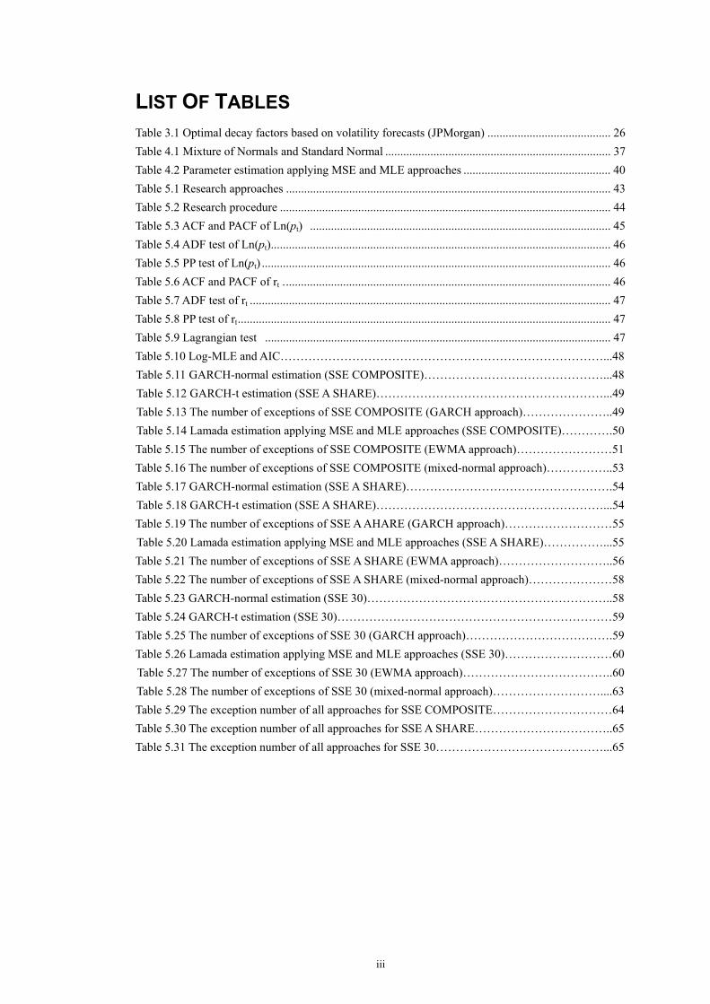
LIST OF TABLES Table 3.1 Optimal decay factors based on volatility forecasts (JPMorgan) ......................................... 26 Table 4.1 Mixture of Normals and Standard Normal ........................................................................... 37 Table 4.2 Parameter estimation applying MSE and MLE approaches ................................................. 40 Table 5.1 Research approaches ............................................................................................................ 43 Table 5.2 Research procedure .............................................................................................................. 44 Table 5.3 ACF and PACF of Ln(pt) .................................................................................................... 45 Table 5.4 ADF test of Ln(pt)................................................................................................................. 46 Table 5.5 PP test of Ln(pt) .................................................................................................................... 46 Table 5.6 ACF and PACF of rt ............................................................................................................. 46 Table 5.7 ADF test of rt ........................................................................................................................ 47 Table 5.8 PP test of rt............................................................................................................................ 47 Table 5.9 Lagrangian test ................................................................................................................... 47 Table 5.10 Log-MLE and AIC………………………………………………………………………...48 Table 5.11 GARCH-normal estimation (SSE COMPOSITE)………………………………………...48 Table 5.12 GARCH-t estimation (SSE A SHARE)…………………………………………………...49 Table 5.13 The number of exceptions of SSE COMPOSITE (GARCH approach)…………………..49 Table 5.14 Lamada estimation applying MSE and MLE approaches (SSE COMPOSITE)………….50 Table 5.15 The number of exceptions of SSE COMPOSITE (EWMA approach)……………………51 Table 5.16 The number of exceptions of SSE COMPOSITE (mixed-normal approach)……………..53 Table 5.17 GARCH-normal estimation (SSE A SHARE)…………………………………………….54 Table 5.18 GARCH-t estimation (SSE A SHARE)…………………………………………………...54 Table 5.19 The number of exceptions of SSE A AHARE (GARCH approach)………………………55 Table 5.20 Lamada estimation applying MSE and MLE approaches (SSE A SHARE)……………...55 Table 5.21 The number of exceptions of SSE A SHARE (EWMA approach)………………………..56 Table 5.22 The number of exceptions of SSE A SHARE (mixed-normal approach)…………………58 Table 5.23 GARCH-normal estimation (SSE 30)……………………………………………………..58 Table 5.24 GARCH-t estimation (SSE 30)……………………………………………………………59 Table 5.25 The number of exceptions of SSE 30 (GARCH approach)……………………………….59 Table 5.26 Lamada estimation applying MSE and MLE approaches (SSE 30)………………………60 Table 5.27 The number of exceptions of SSE 30 (EWMA approach)………………………………..60 Table 5.28 The number of exceptions of SSE 30 (mixed-normal approach)………………………....63 Table 5.29 The exception number of all approaches for SSE COMPOSITE…………………………64 Table 5.30 The exception number of all approaches for SSE A SHARE……………………………..65 Table 5.31 The exception number of all approaches for SSE 30……………………………………...65

iv

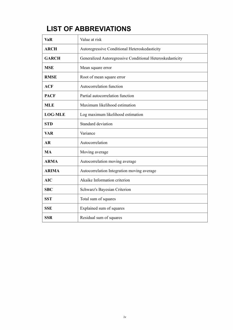
LIST OF ABBREVIATIONS

VaR Value at risk

ARCH Autoregressive Conditional Heteroskedasticity

GARCH Generalized Autoregressive Conditional Heteroskedasticity

MSE Mean square error

RMSE Root of mean square error

ACF Autocorrelation function

PACF Partial autocorrelation function

MLE Maximum likelihood estimation

LOG-MLE Log maximum likelihood estimation

STD Standard deviation

VAR Variance

AR Autocorrelation

MA Moving average

ARMA Autocorrelation moving average

ARIMA Autocorrelation Integration moving average

AIC Akaike Information criterion

SBC Schwarz's Bayesian Criterion

SST Total sum of squares

SSE Explained sum of squares

SSR Residual sum of squares

v

ACKNOWLEDGEMENT This thesis is a fruit work with assistance from many people. I appreciate so much to

my supervisor, Professor Ziyou Yu’s guidance, patience and help. I learnt how do a

research, how to think and how to keep pursuing “better” and study life-long. I

appreciate so much for her willingness to spend so much time on changing my way of

thinking, to be logic. “Thank you” is not enough to express my grateful heart. Learning

from her is my fortune of whole life. I want to present my best regards to Dr Yu, who

cared my study and growth, gave me warm feeling when I was far from home. I also

appreciate so much to Professor Daning Sun. Thanks to his encourages and supports, I

finished my thesis successfully. In addition, I am grateful to all the Professors and

colleagues at the Department of Finance and Insurance and Business School at Lingnan

University.

All my work is with my wife and son. I hereby present my improvements and thesis to

their deep understanding and endless love.

1

CHAPTER 1 INTRODUCTION

1.1 Background

1.1.1 Risk Risk can be defined as the volatility of unexpected outcomes, generally for values of assets

and liabilities (Jorion, 1997). Financial risk relates to possible losses in financial markets

arising from, for example, movements in interest rates and exchange rates. Financial risk can

be divided into the following five types of risk.

Market risk – arises from changes in the prices of financial assets and liabilities and

can be defined as the risk of losses due to adverse market conditions. Market risk can be

absolute, the loss measured in dollar terms, or relative, the loss relative to a benchmark

index.

Credit risk – is defined as the risk of a loss due to the inability of a counterpart to

meet its obligations. Credit risk can lead to losses when debtors are downgraded by

credit agencies, usually leading to a fall in the market value of its obligations.

Liquidity risk – can take two forms: market/product liquidity and cash flow/funding.

The former type of risk arises when a transaction cannot be conducted at prevailing

market prices due to insufficient market activity and poor depth and resiliency in the

market. The latter type of risk is associated with the inability of a firm to fund illiquid

assets or to meet cash flow obligations, which may force early liquidation.

Operational risk – the risk from the failure of internal systems such as management

failure, fraud, and errors made in instructing payments or settling transactions.

Legal risk – risk of changes in regulations or when a counterparty does not have the

legal or regulatory authority to engage in a transaction.

This MPhil thesis is specializing on market risk, which involves the uncertainty of earnings

or losses resulting from changes in market conditions such as asset prices, interest rates,

volatility, and market liquidity (see JP Morgan/RiskMetrics group, 1995, Introduction to

RiskMetrics).

1.1.2 VaR Theory

The primary tool for evaluating market risk is Value at risk (VaR, henceafter), which is a

2

method of assessing risk through standard statistical techniques. Philippe Jorion defines VaR

as a measure for the worst expected loss over a given time interval under normal market

conditions at a given confidence level (Jorion, 1997). Formally VaR is defined as:

∫∞−

=VaR

dxxf )(α or [ ] α=<VaRxPr (1.1)

where α is the significant level, f(x) represents probability distribution of the future

portfolio value; x stands for the change in the market value of a given portfolio over a given

time horizon with the probability. This specification is valid for any distribution, discrete, or

continuous, fat or thin tails (Jorion, 1997).

The factors that determine VaR for a certain asset are the volatility, time horizon and a

choice of confidence level. The volatility is estimated through econometric and statistical

models. The time period chosen affects both the measured volatility and therefore also the

VaR, where a longer time period gives a higher volatility measure and hence, a higher VaR.

The chosen confidence interval states how often the loss on the specific asset will be greater

than the VaR. The most commonly used confidence intervals are 95% and 99% (Danielsson

and de Vries, 1997).

The formula to calculate VaR for one asset is (Jorion, 1997):

VaR = E(W)-W* = -W0*(R*- µ) (1.2)

where W0 is the initial investment, W* is the minimum value, R* is the cutoff return, µ is the

expected return.

In practice, the VaR can be represented as a combination of volatilities and residual

(standardized return) distribution functions. Given the probability density function of the

standardized return, we can define the VaR as

1 ˆ( ) ( )t tVaR α α σ−= Φ (1.3)

3

where ˆtσ represents the conditional standard deviation estimated by at time t. Φ−1 (α) is the

quantile of a standardized normal variable, student-t variable, or other variable with assumed

distribution.

1.1.3 Normal distribution of financial returns

In most theoretical and empirical work regarding financial returns, a normal distribution is

assumed since it simplifies all calculations. In addition, it produces tractable results and all

moments of positive order exist (Lucas and Klaassen,1998). Moreover, the normal

distribution is characterized by its mean and variance and by only knowing these two

variables you know the entire distribution. A normal distribution can be defined by the

density function below:

−−= 2

2

2 2)(

exp2

1)(σµ

πσt

tr

rf (1.4)

Where tr is a random variable, µ is the mean and 2σ is the variance of tr .

However, these advantages have to be weighed against research showing that the

distribution of returns in financial markets experience fat tails (Hendricks, 1996). Financial

returns generally exhibit leptokurtic behavior and extreme price movements occur more

frequently than what is given by the normal distribution (see JPMorgan/Reuters, 1996,

RiskMetrics – Technical Document). A leptokurtic distribution implies that the distribution

has a high peak, the sides are low and the tails are fat.

Since VaR is concerned with unusual outcomes, the fact that tails are fat poses a problem.

More outcomes than predicted by the normal distribution will fall into the category that

exceeds the VaR measures generated with normal distribution, i.e. the assumption of normal

distribution underestimates the VaR (Lucas and Klaassen, 1998).

4

1.1.4 Skewness and Kurtosis

The normal distribution is symmetric with the mean equal to the median. Departure from

symmetry usually implies a skewed distribution. Skewness is a measure of the degree of

asymmetry of a frequency distribution. Positive skewness, or right-skewed, is an indication

of a distribution with an asymmetric side that is expanding towards more positive numbers.

Negative skewness, or left-skewed, implies the opposite, i.e. a distribution that stretches

asymmetrically to the left (Aczel, 1993). The formula for skewness is:

3

111

2)( ∑

=

−

−

−=

n

i x

i

sxx

nnnxSk (1.5)

where xs is the standard deviation, n is the number of observations, xi is the observed

variable at time i and x is the mean of all observations (Kleinbaum, Kupper and Muller,

1988).

Kurtosis is a measure of the flatness versus peakedness of a frequency distribution. In

statistics flat is called platykurtic and peaked is called leptokurtic. A positive kurtosis

indicates a relatively leptokurtic distribution, while a negative kurtosis indicates a relatively

platykurtic distribution (Aczel, 1993). The formula to calculate the kurtosis is the following

(Kleinbaum, Kupper and Muller, 1988):

4

111

)3)(2()1()( ∑

=

−

−

−−

+=

n

i x

i

sxx

nnnnnxKur (1.6)

Out of an asset manager perspective the portfolio risk is one of the most decisive parameters

to have perfect control over. A well-functioning VaR measurement method could therefore

be a superior way to supervise the portfolio risk and quantify potential losses. The greatest

benefit of VaR for an asset manager, according to Philippe Jorion, probably lies in the

imposition of a structured methodology for critically thinking about risk. Institutions

applying VaR are forced to confront their exposure to financial risk. A well- functioning

supervision of VaR should logically also imply less risk of unexpected and uncontrolled

losses.

5

1.2 Research Objective As is well known, most parametric VaR models use a normal distribution to characterize the

distribution of returns, and historical returns are used to make predictions about the future.

However, when the financial markets are experiencing stress, the hypothetical normal

distribution may not reflect the real situation and thus may not be able to make a good

predication for the outcomes. Lucas and Klaassen showed that the normal distribution

underestimates VaR by more than 30 percent at the 99% level under normal market

conditions (Lucas and Klaassen, 1998). Research has found that financial returns experience

fat tails, which implies that the normal distribution works well in predicting frequent

outcomes but is not a good estimator to predict extreme events (Dowd, 1999). In addition,

Venkataraman (1996) and Zangari (1996) argued that normal distribution cannnot

accommodate the observed skewness and the kurtosis of the financial time series.

The purpose of this thesis is to verify which method including methods using RiskMetrics,

Generalized Autoregressive Conditional Heteroscedasticity (GARCH) models, and

Exponential weighted moving average (EWMA) with a mixture of normal distributions is

better as a reliable and stable risk measurement tool for the Chinese stock markets, and to

find an appropriate VaR method for the Chinese asset managers to supervise the portfolio

risk and quantify the potential losses. This thesis compares the RiskMetrics (JP Morgan,

1996) and the GARCH-type models in order to estimate one-day VaR for three diversified

index portfolios including Shanghai Stock Exchange Composite Index (SSE COMPOSITE),

Shanghai Stock Exchange A Share Index (SSE A SHARE) and Shanghai Stock Exchange 30

Index (SSE 30) at 95% and 99% confidence level. Practically, the fitting of VaR measures

computed by the RiskMetric model and an alternative set of GARCH (p,q) models are

compared. The analysis includes the comparison among the fitted models based on all

results evaluated using backtesting performance criteria. Further on, EWMA approach with

mixed normal distributions is proposed and compared with GARCH-typed models and

EWMA. In detail, firstly, the probability density function for conditional variance is

assumed to be 2 2)1 1 1 1 1 2 2 2( ) ( , , ) (1 ( , , )f x p x p xφ µ σ φ µ σ= + − , where φ is the probability

density function of normal distribution. We use MLE to estimate the five parameters and get

the density function. Then we use the definition of VaR to calculate the quantile value for

standardized return. We can multiply the quantile value by conditional standard deviation to

get VaR.

The combination of VaR for Chinese stock and the risk topics is very appealing, which

explains the choice of subject for this MPhil thesis. From the discussion above, the

6

following questions are asked:

Is VaR (either RiskMetric model or GARCH-typed modesl) a useful tool for the

Chinese asset managers to monitor risk?

Which VaR method (RiskMetric model or GARCH-typed modes or EWMA with mixed

normal distributions) is more reliable as a risk measurement tool for Chinese equity

portfolios?

1.3 Feature of our research Even if some research papers similar have reported studies to the thesis, there are significant

differences ought to be mentioned. First, some previous studies in this area have mostly

focused on the developed financial markets. There are some studies regarding VaR in

Chinese financial markets. However, when applying RiskMetrics approach, most researches

used the decay factor (lamada) proposed by J.P. Morgan directly (0.94 daily and 0.97

monthly). Instead, we obtained the lamada by minimizing the Mean Square Error (MSE). At

the same time, we also estimate the lamada using Maximum Likelihood Estimation (MLE).

Further more, we compared these two approaches using the same data set.

Second, we employed the single state distribution and the mixed state distribution

parametric techniques in order to investigate their performance in a unified environment, in

contrary to the existent literature, which, to the best of our knowledge, focused only on

single state. Moreover, we compared EWMA approach with the combined normal

distribution with GARCH-type models. For this mixed state distribution approach, it is not

as complex as GARCH, but it considers heteroscedasticity and fat-tail effect, as well as

skewness and kurtosis.

Third, a clear procedure is developed to determine which GARCH specification is the most

appropriate. Briefly, we first ignored the heteroscedasticity and worked only on the mean

equation and determined the optimal lags in ARIMA. Then, based on the "optimal"

specification of mean equation, we proceeded to work with the GARCH part. We used the

MLE and AIC to determine the GARCH specification under the consideration of the

principle of parsimony. In detail, some Chinese scholars got the GARCH (p, q), where p>3,

q>=2. It is important to note that in practice the GARCH (1, 1) has been adequate for many

processes. In journal articles in, say, Journal of Applied of Econometrics, Journal of

Econometrics, and the like, people do not think about GARCH (p, q), where p>3, q>=2. For

concreteness, if we end up with a GARCH (3, 3), that may be unusual. In this thesis, we

choose GARCH (1, 1) specification as our favorite specification for conditional variance

models since it has been adequate for our research. Besides, considering that we have 1564

observations, there is no much difference between the Log-likelihood/AIC of GARCH (1, 1)

7

and GARCH (2, 2), the one with the highest maximum likelihood and the lowest AIC value.

1.4 Organization of the Thesis There are six chapters in this thesis. Chapter 1 introduces the research background and the

research objective. Chapter 2 reviews the literature related to all methods to calculate VaR

and the hypothesis-testing framework. Chapter 3 introduces the research framework.

EqWMA, EWMA, GARCH-typed models are introduced briefly. Some econometric

concepts including ACF, PACF, unit root test, AIC, are explained in this part. Chapter 4 is

the research methodology part. This part explains how to use MLE to estimate the

parameters of EWMA approach with a mixture of normal distributions, and compares the

MLE used in GARCH specification with the optimization method of minimizing MSE in

EWMA approach. Then these two approaches are applied to calculate the optimal decay

factor using China financial markets data. Chapter 5 is the data analysis part. We first briefly

introduce our procedure of data processing and model estimating. Then we calculate the

conditional variance and quantile for standardized return, and hence the VaR. In addition,

different approaches are compared under the Hypothesis-testing framework. In chapter 6, the

conclusion, suggestions for further study and the contributions of this study are introduced.

8

CHAPTER 2 LITERATURE REVIEW

2.1 Introduction Value at risk (VaR) has gradually become popular in risk management since it is an easily

understood and obviously concept to describe risk. Jorion (2000) provides an introduction to

value at risk and discusses its estimation. The www.gloriamundi.org website

comprehensively cites the value at risk literature.

Although explaining the concept of VaR is easy, creating the value is non-trivial. In

statistical terms, the task is to provide a given quantile for a portfolio return distribution that

is continuously changed and unobservable. In practice, VaR can be calculated as follows:

First, we need to calculate the variance. Since a distribution that is continuously changed and

unobservable, conditional variance is normally used. Second, we need to calculate the

percentile (95% and 99%) under some parametric distribution assumption (for standardized

return) at a given confidence level. Then we can multiply the conditional standard deviation

by the percentile to get VaR. In addition, since the task is complex, it is necessary to test the

quality of the procedures that are proposed. Hypothesis-Testing Framework proposed by

Kupiec (1995) is often used for this purpose.

In this chapter, we reviewed the relevant scholarly literatures including dissertations and

conference proceedings as well as business newsletters related to the topic of VaR research

models, constructs and measurements, methodologies for creating and testing VaR.

2.2 VaR estimation methods In order to calculate the VaR number, one can use parametric, non-parametric or

semi-parametric methods. The parametric, or namely the variance-covariance, involves

specifying a parametric distribution and estimating the parameters with historical data.

Based on the estimated distribution, one can calculate the conditional variance and

appropriate quantile. On the other hand, the nonparametric or portfolio approach involves

constructing the distribution of portfolio returns that mimic the past performance of the

portfolio (Wang, 2000).

2.2.1 Parametric method Many researchers prefer parametric methods since it is convenient to model the underlying

distribution. For parametric methods, we can calculate VaR for given distribution

assumptions, such as normal, t, and mixed normal distributions. Parametric method can be

classified in two categories, single state distribution and mixed state distribution approaches.

9

2.2.2.1 Single state distribution approach In the single state case, normal distribution is most often assumed. Some researches

proposed t-distribution since the latter can describe fat-tail more appropriately than normal

distribution. However, some people suggest that t-distribution is superior to normal at high

confidence level, say 99%, but normal distribution is god enough at 95% confidence level or

lower,. There are extensive literatures on models describing volatility under single state

distribution assumption.

Brooks and Persand (2003) consider the issue of the asymmetry in the VaR framework and

concluded that models, which do not allow for asymmetries in the volatility specification,

underestimate the “true” VaR. Angelidis, Benos, and Degiannakis (2003) evaluated the

performance of an extensive family of ARCH models in modelling daily VaR of perfectly

diversified portfolios in five stock indices, using a number of distributional assumptions and

sample sizes. Moreover, after comparing the skewed generalized-t distribution with 10

GARCH specifications, Bali and Theodossiou (2004) pointed out that the TS-GARCH,

proposed by Taylor (1986) and Schwert (1989), and the EGARCH, introduced by Nelson

(1991), performed best among all the models.

2.2.2.2 Mixed state distribution approach Mixture of normal distribution, which takes into account the skewness and kurtosis, is a

more flexible distribution for fitting the market data of daily changes. Actually, the normal

distribution is a special case of the mixture of normal distributions. For a mixture of normal

distributions with identical mean and variance, it is a normal distribution. Mixture of

normals has continued to receive increasing attention (McLachlan and Peel [2000]). This

model has been successfully applied in many fields including economics, marketing, and

finance (Clark [1973], Zangari [1996], Venkataraman [1997], Due and Pan [1997], Hull and

White [1998], and Wang [2000]). The mixture of normal distributions has become a popular

model for the distribution of daily changes in market variables with fat tails, skewness and

kurtosis.

In this case, Venkataraman (1996) and Zangari (1996) showed that the distributions of daily

changes, such as returns in equity, foreign exchanges, and commodity markets, are

frequently asymmetric with fat tails. The assumption of normality is far from perfect and

often inappropriate. They suggested the market practitioners to use a mixture of normal

distributions which can accommodate the observed skewness and the kurtosis of the

financial time series and hence can describe them better than the normal distribution. Billio

and Pelizzon (2000) estimated a multivariate switching regime model to calculate the VaR

for 10 Italian stocks and for several portfolios. They concluded that the switching regime

10

specification is more accurate than the other known methods (RiskMetricsTM or Garch (1,1)

under Normal and Student-t distribution).

The key step of this approach is to fit parameters to a mixture of normal distributions. A

variety of approaches have been used to estimate mixture of normal distributions. They

include the method of moments, maximum likelihood, and Bayesian approaches. A detailed

overview can be found in Titterington, Smith, and Makov [1985], and McLachlan [2000].

The method of maximum likelihood (MLE) is the most widely preferred method to the

estimation problem of a mixture of normals (Wang 2000).

2.2.2 Non-parametric methods Historical simulation (HS) is a non-parametric VaR-method which assumes that historical

returns are a good guide for future returns. The HS does not rest on the assumption about

normally distributed returns, but on an empirical distribution of returns. In addition, the

distribution of the returns in the portfolio should be constant over the sample period

(Danielsson, 1997). In other words, there should be no structure break in this period.

HS has been thoroughly examined. The sample size is the key issue in this approach. Frey

and Michaud (1997), Hoppe (1998) proposed the use of a smaller one, since it can

accommodate the structural changes of the trading behaviour. However, Hendricks (1996),

Vlaar (2000) and Dan´ielsson (2002) argued that the sample size affects the precision of the

VaR estimates, with the longer one producing the most accurate estimations.

2.2.3 Mixture of parametric and non-parametric methods Besides historical simulation and variance-covariance techniques, there are also models

based on mixture of parametric and non-parametric approach.

Hull and White (1998) and Barone-Adesi et al. (1999) proposed the filtered historical

simulation (FHS) to combine the historical simulation and the variance-covariance method.

This volatility model is without any distributional assumption about the standardized returns.

Moreover, Barone-Adesi and Giannopoulos (2001) demonstrated that the performance of the

filtered historical simulation is better than that of historical one since it generated better VaR

forecasts than the latter method.

Under the same framework, the Extreme Value Theory (EVT) has been proposed recently,

which models only the tails of the distribution rather than the entire one. Therefore, it

focuses on the parts of the distribution that are essential for the VaR.

11

2.3 Hypothesis-Testing Framework In order to evaluate the VaR forecasts from the actual VaR, we normally use

hypothesis-testing framework since the latter is unobservable and a direct comparison

between them can not be made. Evaluation methods based on a hypothesis-testing allow us

to test the null hypothesis that VaR forecasts are “acceptably accurate.”

For hypothesis-testing framework, the null hypothesis is that VaR forecasts in question

exhibit a specified property or characteristic of accurate VaR forecasts (Lopez, 1998). If the

null hypothesis is rejected, the VaR forecasts do not exhibit the specified property, and the

underlying VaR model can be said to be “inaccurate.” If the null hypothesis cannot be

rejected, the model is said to be“acceptably accurate.”

The most commonly used hypothesis-testing technique is unconditional coverage framework

firstly proposed by Kupiec (1995). Kupiec constructed VaR verification tests from the series

of Bernoulli trial outcomes generated by a daily performance comparison. That is, treat the

loss on trading activities less than the VaR estimated as a success, and beyond the VaR as a

failure (Kupiec, 1995). To be more specially, the most basic requirement of a VaR model is

that the proportion of times that the VaR forecast that it generates is exceeded (the number of

exceptions) should on average equal the nominal significance level, in other words the

model should provide correct unconditional coverage (Kupiec, 1995).

In order to test the null hypothesis that the unconditional coverage is equal to the nominal

significance level, Kupiec (1995) has derived an LR (Likelihood Ratio) statistic based on the

observation that the probability of observing N exceptions in a sample of size T is governed

by a binomial process and is given by NNT pp −− )1( . The LR statistic, which is chi-square

distribution with one degree of freedom, is computed as

})()](1ln{[2])1ln[(2 NTNNT

TNNNT

uc ppLR −− −+−−= (2.1)

where p is the desired significance, T is the total number of days in the whole period, N is

the the number of days on which the predicted VaR exceeds the actual VaR.

2.4 Related research in the Chinese financial markets Our research will focus on the China financial markets, so it is necessary to review research

conducted in the Chinese financial markets.

Financial issues related to China exemplify many intriguing characteristics of an emerging

12

financial market, which differs from the western well-developed financial markets. Laurence,

Cai, and Qian (1997) and Liu, Song, and Romily (1996) provide early studies on the

weak-form efficiency of the Chinese stock market. Using serial correlation tests, Laurence et

al conclude that the domestic A-share markets are weak-form efficient, while the B-share

market in Shanghai is not efficient. Liu et al find (1) each stock exchange (SHSE and SZSE)

share price index follows a random walk process; (2) there is cointegration between these

two indexes; and (3) there is bidirectional causality between these two indexes. Su and

Fleisher (1998) investigate the risk-return behavior of the Chinese stock market in light of

government regulation. Relative to the markets in the developed countries, they find that risk

adjusted return in Chinese stock market is low and volatility of returns is very high and

time–varying. Friedmann and Sandford-Kohle (2000) analyze volatility dynamics using

GARCH type models in the Chinese stock market. They find that bad news increase

volatility more than good news in A-share indices and Composite indices, whereas good

news increases volatility more than bad news in B-share indices. Lee, and Rui (2001) use a

different methodology to investigate the relation between stock return and volatility. The

results of GARCH and EGARCH models suggest there is a time-varying volatility but no

relation between expected return and expected risk level. Su (2003) investigates whether

corporate earnings disclosures convey information in the Chinese stock market. Su reports

significant abnormal returns for A-share market and little or no abnormal returns for B-share

market on the announcement date. Some of the findings in the Chinese stock market are

similar to those in the developed stock market, and some other results are very different.

These mixed findings indicate that China indeed has a different economic, institutional, and

market microstructure.

Ang Niu(1997), Gang Yao(1998),Naikang Gu(1998), Jianguo Chan(1998), Yaoting Zhang

(1998), Xingquan Liu(1999), Yuanrui Zhan(1999), Wende Pan(1999), Wentong Zheng(1999),

Yufei Liu(1999), Jun Tian(2001) discussed the principles and application of VaR , and

introduced historical simulations, Monte-Carlo and variance-covariance methods. Zhihui

Li(2001), Naquan Jiang(2003)discussed mean-variance investment model under VaR

constraint. Haitao Du(2000) proved that RiskMetric model is a relatively reliable risk

measurement tool in Chinese stock market. Ling Zhao(2002) theoretically analyzed the

optimal portfolio selection model under VaR Constraint.

At present stage, there are some studies regarding VaR in Chinese equity market, but most

empirical work only use models based on single state distribution. We detect this gap and

conduct thorough comparisons among RiskMetrics, GARCH-typed models and EWMA

based on mixed normal distribution. In addition, we use MLE and MSE to estimate the

decay factor for Chinese stock markets in RiskMetrics approach and make comparisons

13

between these two methods.

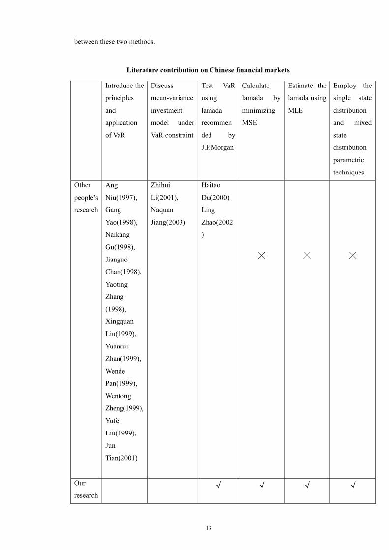
Literature contribution on Chinese financial markets

Introduce the

principles

and

application

of VaR

Discuss

mean-variance

investment

model under

VaR constraint

Test VaR

using

lamada

recommen

ded by

J.P.Morgan

Calculate

lamada by

minimizing

MSE

Estimate the

lamada using

MLE

Employ the

single state

distribution

and mixed

state

distribution

parametric

techniques

Other

people’s

research

Ang

Niu(1997),

Gang

Yao(1998),

Naikang

Gu(1998),

Jianguo

Chan(1998),

Yaoting

Zhang

(1998),

Xingquan

Liu(1999),

Yuanrui

Zhan(1999),

Wende

Pan(1999),

Wentong

Zheng(1999),

Yufei

Liu(1999),

Jun

Tian(2001)

Zhihui

Li(2001),

Naquan

Jiang(2003)

Haitao

Du(2000)

Ling

Zhao(2002

)

╳

╳

╳

Our

research

√ √ √ √

14

CHAPTER 3 RESEARCH FRAMEWORK

3.1 Introduction

This chapter introduces the framework of our research. Based on the existing theories in risk

management and time series econometrics, we will provide background for our research

methodology in Chapter 4. This part will introduce the Equally Weighted Moving Average

Approach (EqWMA), the Exponentially Weighted Moving Average Approach( EWMA),

GARCH-typed models very briefly, as well as explaining some basic econometric concepts

including unit root test, ACF, PACF, and AIC.

3.2 VaR estimation models

In the following part, EqWMA, EWMA and GRACH-typed models are introduced briefly.

3.2.1 The equally weighted moving average

The equally weighted moving average (EqWMA) approach assumes an unconditional

normal distribution for the probability density function of equity return and uses a fixed

amount of historical data to calculate the standard deviation. The calculation of the standard

deviation is:

∑−

−=

−−

=1

2)()1(

1 t

ktsst x

kµσ (3.1)

where tσ is the estimated standard deviation at time t, and k specifies the number of

observations included in the moving average. xs is the change in the value of the asset on day

s and μis the mean change in asset value during the estimated period (Hendricks, 1996).

For shorter periods of time, the standard deviation gets more irregular and reacts faster to

changes in asset price movements. The other parameters that have to be set is the confidence

interval. The most commonly used confidence levels are the 95th and the 99th percentile

(Hendricks, 1996).

An advantage with the EqWMA approach is that it is easy to use, since the normal

distribution is only characterized by its mean and variance. Many statistical formulas are

15

based on a normal distribution assumption and these facilitate the analysis of the results

(Lucas and Klaassen, 1998).

The most obvious disadvantage with the EqWMA approach, as mentioned above, is that

financial returns experience fat tails. Therefore using a normal distribution underestimates

the true VaR, which of course is a very serious drawback (Danielsson, 1997). Another

disadvantage is that the EqWMA approach gives the same weight to all the observations

instead of putting more weight on recent data.

3.2.2 The Exponentially Weighted Moving Average Approach

In contrast to the EqWMA approach, the exponentially weighted moving average (EWMA)

approach attaches different weights to past observations in the observation period (Jorion,

1997). The weights decline exponentially and therefore, the most recent observations get

much higher weight than earlier observations. The formula for the standard deviation under

the ExpWMA is shown below:

2

112 ))(1( µλλσσ −−+= −− ttt x (3.2)

where tσ and 1tσ − are the estimated standard deviations at time t and t-1, respectively,

and k specifies the number of observations included in the moving average. 1tx − is the

change in the value of the asset on day t-1 and μis the mean change in asset value during

the estimated period.

The parameter λ (lambda) determines at which rate past observations decline in value as

they become more distant (Hendricks, 1996). Formula (3.2) shows that on any given day the

standard deviation, calculated as an exponentially moving average, consists of two

components. One is the weighted average variance of the previous day. The other is

yesterday’s squared deviation, which is given a weight of (1-λ ). This means that a lower

value on λ makes the importance of observations decline at a more rapid speed (Hendricks,

1996).

16

3.2.2.1 What value of lamada should be used?

A low decay factor implies that almost the entire VaR measure is derived from the most

recent observations. This means that the VaR measure becomes very volatile over time. On

the one hand, relying on the most recent observations is important for capturing short-term

movements in volatility. On the other hand, a smaller sample size increases the possibility of

measurement error (Hendricks, 1996).

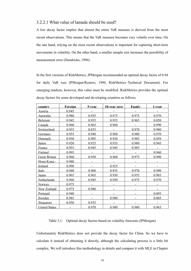
In the first versions of RiskMetrics, JPMorgan recommended an optimal decay factor of 0.94

for daily VaR (see JPMorgan/Reuters, 1996, RiskMetrics–Technical Document). For

emerging markets, however, this value must be modified. RiskMetrics provides the optimal

decay factors for some developed and developing countries as follows.

country Foreign 5-year 10-year zero Equity 1-year Austria 0.945 - - - -Australia 0.980 0.955 0.975 0.975 0.970Belgium 0.945 0.935 0.935 0.965 0.850Canada 0.960 0.965 0.960 - 0.990Switzerland 0.955 0.835 - 0.970 0.980Germany 0.955 0.940 0.960 0.980 0.970Denmark 0.950 0.905 0.920 0.985 0.850Spain 0.920 0.925 0.935 0.980 0.945France 0.955 0.945 0.945 0.985 -Finland 0.995 - - - 0.960Great Britain 0.960 0.950 0.960 0.975 0.990Hong Kong - 0.980 - - - -Ireland 0.990 - 0.925 - -Italy 0.940 0.960 0.935 0.970 0.990Japan 0.965 0.965 0.950 0.955 0.985Netherlands 0.960 0.945 0.950 0.975 0.970Norway 0.975 - - - -New Zealand 0.975 0.980 - - -Portugal 0.940 - - - 0.895Sweden 0.985 - 0.980 - 0.885Singapore 0.950 0.935 - - -United States - 0.970 0.980 0.980 0.965

Table 3.1: Optimal decay factors based on volatility forecasts (JPMorgan)

Unfortunately RiskMetrics does not provide the decay factor for China. So we have to

calculate it instead of obtaining it directly, although the calculating process is a little bit

complex. We will introduce this methodology in details and compare it with MLE in Chapter

17

4.

3.2.2.2 Advantages and disadvantages with the ExpWMA approach

The advantages with the EWMA approach are very much the same as with the EqWMA

approach. However, the volatility is much more receptive to variations over time. For an

exponential moving average, the standard deviation is responsive to market shocks and the

following gradual decline in the forecast of volatility. However, a simple moving average

does not react fast enough to changes in the volatility (JPMorgan/RiskMetrics group, 1995,

Introduction to RiskMetrics).

The disadvantage is that this approach does not fully consider the fat tail, skewness and

kurtosis, although it assumes a conditional normal distribution to describe the volatility over

time. In addition, the computations are somewhat more difficult and that the volatility over

time is more unstable than with the EqWMA approach (see JPMorgan/Reuters, 1996,

RiskMetrics–Technical Document). But the computation task is easy to handle with

statistical software package, such as Eview, SAS, GAUSS, and Matlab.

3.2.3 GARCH-typed models

GARCH models were introduced by the seminal works of Engle (1982) and Bollerslev

(1986). These models tried to explain several empirical findings of financial market series.

The main innovation was in the modelization of the conditional variances that were

structured with a time-dependent relation (Massimiliano and Greta, 2003).

The model can be represented with mean equation and variance equation. The mean

equation is as follows:

tttt zIy σµ += − )( 1

[ ] 01 =−tt IZE [ ] 112 =−tt IZE (3.3)

where tz is a standard normal distribution; 1tI − is mean equation at the time t-1.

in this case the standardized residual are coherent with a standardized normal distribution,

18

however other assumptions can be made, including the Student-t distribution and the GED

(Generalized Error Distribution).

The conditional variances are defined (Massimiliano and Greta, 2003):

∑∑=

−

=

−− ++=q

jjtj

p

iititit z

1

2

1

22 σβσαωσ (3.4)

where 1tz − is a standard normal distribution, ω , α , and β are three parameters for

estimation. The representation considered is the GARCH (p,q).

We can easily see that EWMA is a special case of GARCH under two assumptions. First, in

the mean equation, the mean is identically equal to zero, µ(It−1) = 0. Second, in the variance

equation, p,q are both equal to unity, the sum of a and B is equal to unity, and ω , the

intercept, is equal to zero.

Within GARCH-type models, the conditional volatilities play an essential role in the

computation of VaR levels. In fact, the VaR can be represented as a combination of

volatilities and residual distribution functions. In particular, assuming also that we know the

probability density function of the standardized residuals (given any GARCH model, these

are equal to the mean residuals divided by the conditional volatilities), the VaR can be

represented as (Massimiliano and Greta, 2003)

1 ˆ( ) ( )t tVaR α α σ−= Φ (3.5)

where Φ−1 (α) is the quantile of a standardized normal variable, student-t variable, or other

variable with assumed distribution. ˆtσ represents the conditional standard deviation

obtained at time t(Massimiliano and Greta, 2003).

Behind the GARCH-models lies an assumption of time-varying conditional volatility. The

GARCH (p,q) model successfully captures volatility clustering of financial time series, as

noted by Mandelbrot (1963): “. . . large changes tend to be followed by large changes of

either sign, and small changes tend to be followed by small changes. . . ”.

19

On the other hand, GARCH does not fully consider skewness and kurtosis, although it

assumes a conditional normal or student-t or other known distribution to describe the

volatility over time and the fat-tail effects. In addition, the GARCH structure presents some

drawbacks on implementation, since it requires large numbers of observations to produce

reliable estimates. In other words, GARCH-type models represent a more reliable solution

and a better efficiency at the higher level of complexity.

3.3 Some concepts in time series econometrics

Let pt represents the price index of stock return at the time of t. Normally we use

rt=logpt-logpt(-1). In chapter 5, we will explain why we define stock return in this form.

Some related concepts are introduced in this section.

3.3.1 Autogressive moving average

We have mentioned the mean equation, i.e. Autoregressive-moving-average (ARMA), in

GARCH-typed models. Actually we call it an Autoregressive-integrated-moving-average

(ARIMA) if the difference equation has at least one unit root equal to or bigger than unity.

This part will introduce ARMA model which are mathematical models of the persistence, or

autocorrelation, in a time series.

3.3.1.1 Mathematical Model

ARMA models can be described by a series of equations. The equations are somewhat

simpler if the time series is first reduced to zero-mean by subtracting the sample mean.

Therefore, we will work with the mean-adjusted series

, 1, 2....t ty Y Y t N= − = (3.6)

Where tY is the original time series, Y is its sample mean, and ty is the mean-adjusted

series. One subset of ARMA models are the so-called autoregressive, or AR models. An AR

model expresses a time series as a linear function of its past values plus a noise term. The

order of the AR model tells how many lagged past values are included. The simplest AR

model is the first order autoregressive, or AR(1), model. The equation for this model is

20

1 1t t ty a y e−− = (3.7)

where ty is the mean-adjusted series in year t, 1ty − is the series in the previous year, 1a is

the lag 1 autoregressive coefficient, and te is the noise. The noise also goes by various

other names: the error, the random-shock, and the residual. The residuals te are assumed to

be random in time (not autocorrelated), and normally distributed. The equation for the AR(1)

model can be rewritten as

1 1t t ty a y e−= + (3.8)

Higher-order autoregressive models include more lagged t y terms as predictors. For

example, the second-order autoregressive model, AR(2), is given by

1 1 2 2t t t ty a y a y e− −= + + (3.9)

where 1a , 2a are the autoregressive coefficients on lags 1 and 2. The pth order

autoregressive model, AR(p) includes lagged terms on years t −1 to t−p. Our research only

involve AR (1) process.

The moving average (MA) model is a form of ARMA model in which the time series is

regarded as a moving average (unevenly weighted) of a random shock series te . The

first-order moving average, or MA(1), model is given by

1 1t t ty e c e −= + (3.10)

Where te , 1te − are the residuals at times t and t-1, and 1c is the first-order moving average

coefficient. Like the AR models, higher-order MA models include higher lagged terms. The

letter q is used for the order of the moving average model. The second-order moving average

model is MA(q) with q = 2.

For example, the second order moving average model, MA(2), is

1 1 2 2t t t ty e c e c e− −= + + (3.11)

We have seen that the autoregressive model includes lagged terms on the time series itself,

and that the moving average model includes lagged terms on the noise or residuals. By

21

including both types of lagged terms, we arrive at what are called

autoregressive-moving-average, or ARMA, models. The order of the ARMA model is

included in parentheses as ARMA (p,q), where p is the autoregressive order and q the

moving-average order. The simplest, and most frequently used ARMA model is AR(1) and

ARMA(1,1) model

AR(1): 1 1t t ty a y e−= + (3.12)

ARMA(1,1) 1 1 1 1t t t ty a y e c e− −= + + (3.13)

Our research only involve AR (1) process.

3.3.1.2 Steps in modeling

ARMA modeling proceeds by a series of well-defined steps. The first step is to identify the

model. Identification consists of specifying the appropriate structure (AR, MA or ARMA)

and order of model. We can conduct it in two steps. First, we look at plots of the

autocorrelation function (ACF) and partial autocorrelation function (PACF) and find

different possible model structures and orders. Second, identification is done by an

automated iterative procedure -- fitting possible models and using a goodness-of-fit statistic,

say AIC, to select the best model.

The second step is to estimate the coefficients of the model. In practice, estimation is fairly

transparent to the user, as it accomplished automatically by a computer program with little or

no user interaction. The third step is to check the model. It includes two important elements;

that is to ensure that the residuals of the model are random, and to ensure that the estimated

parameters are statistically significant.

Moreover, the fitting process is guided by the principal of parsimony, by which the best

model is the simplest possible model that adequately describes the data. The simplest model

is the model with the fewest parameters.

3.3.2 Unit root test

The classical regression model requires that the dependent and independent variables in a

22

regression be stationary. To decide whether a time series is stationary, we normally use unit

root test. A unit root test tests whether a unit root is present in an autoregressive model. The

most famous test is the Dickey-Fuller (DF) test and the augmented Dickey-Fuller (ADF)

tests. Another test is the Phillips-Perron test.

3.3.2.1 Dickey-Fuller (DF) test

Suppose a simple AR(1) model is 1t t ty y uρ −= + , where yt is the variable of interest, t is the

time index, ρ is a coefficient, and ut is the error term. A unit root is present if 1ρ ≥ .

The regression model can be written as 1 1( 1)t t t t ty y u y uρ δ− −∆ = − + = + , where ∆ is

the first difference operator. This model can be estimated and testing for a unit root is

equivalent to testing 0δ = .

3.3.2.2 Augmented Dickey-Fuller (ADF) test

For the ADF tests, three different regression equations are considered.

2

p

t t i t i t i ti

y y y uα δ θ β− −=

∆ = + + + ∆ +∑ (3.14)

2

p

t t i i t i ti

y y y uα δ β− −=

∆ = + + ∆ +∑ (3.15)

2

p

t t i i t i ti

y y y uδ β− −=

∆ = + ∆ +∑ (3.16)

The first equation includes both a drift term and a deterministic trend; the second excludes

the deterministic trend; and the third does not contain an intercept or a trend term. In all three

equations, the parameter of interest is δ . Ifδ = 0, the ty sequence has a unit root. The

estimated t-statistic is compared with the appropriate critical value in the Dickey-Fuller

tables to determine if the null hypothesis is valid.

We also conduct the Phillips-Perron (1988) test for a unit root. This is because the DF or

ADF tests require that the error term be serially uncorrelated and homogeneous while the

23

Phillips-Perron test is valid even if the disturbances are serially correlated and heterogeneous.

In general PP test is preferred to the ADF tests if the diagnostic statistics from the ADF

regressions indicate autocorrelation or heteroscedasticity in the error terms.

3.3.3 ACF and PACF

As mentioned before, ACF and PACF will be used to find different possible ARMA model

structures and orders. But for a unit root process and a stationary process with the

characteristic root close to unity, ACF usually cannot tell the difference.

Autocorrelation is the correlation between observations of a time series separated by say, k

time units. Suppose there are n time based observations, X1, X2, X3, ....., Xn, ACF technique

finds correlation between the observations for different lags.

1

2

1

( )( )

( )

N k

i i ki

k N

ii

Y Y Y Yr

Y Y

−

+=

=

− −=

−

∑

∑ (3.17)

PACF technique is used to compute and plot the partial autocorrelations of a time series.

With PACF we can find correlation between some components of the series, eliminating the

contribution of other components. Put it simple, PACF is the parameter of Yi when we run

multiple regression of Yi+k on Yi…. Yi+k-1.

Here are some general guidelines for identifying the AR (1) process using ACF and PACF:

Autoregressive processes have an exponentially declining ACF and spikes in the first

lag of the PACF. The number of spikes indicates the order of the autoregression.

Nonstationary series have an ACF that remains significant for half a dozen or more lags,

rather than quickly declining to zero. Such a series must be differentiated until it is

stationary.

3.3.4 Akaike information criterion (AIC)

The Akaike information criterion (AIC) is a statistical model fit measure. It quantifies the

24

relative goodness-of-fit of various previously derived statistical models, given a sample of

data. The driving idea behind the AIC is to examine the complexity of the model together

with goodness of its fit to the sample data, and to produce a measure which balances

between the two.

Engle and Yoo (1987) suggest to select ARMA model with the lowest AIC value. We just

follow their conclusion in our research, as most econometricians do. For example, AR (1)

and ARMA(1,1) are two potential models we want to use for the mean equation. To decide

which one is better, we can compare their AIC value and select the one with the smaller

value. For AIC, its formula is AIC = 2k − 2ln(L), where k is the number of parameters, and L

is the likelihood function.

A model with many parameters will provide a very good fit to the data, but will have few

degrees of freedom and be of limited utility. This balanced approach discourages overfitting.

The preferred model is that with the lowest AIC value. The AIC methodology attempts to

find the model with fewest parameters, and at the same time, correctly explaining the data.

25

CHAPTER 4 RESEARCH METHODOLOGY

4.1 Introduction

Chapter 4 introduces our research methodology. In this part, we use MLE to estimate the

parameters of EWMA with a mixture of normal distributions. Also, we compare the MLE

used in GARCH with the optimization method of minimizing MSE in EWMA approach, and

get the conclusion that different parameters can be fitted for different approaches.

4.2 Estimation of the mixed normal distributions

While GARCH-typed models are successful models to describe asset returns, they are also

considerably complicated by practitioners. And these models with single-state distribution

usually do not consider skewness and kurtosis. Moreover, GARCH-type models are not

good at handling multivariate VaR estimation. So we can use the RiskMetrics framework

developed by JP Morgan, as well as a simple version of the mixture of normals approach

proposed by Zangari (1996).

Below, we discuss the mixture of normals approach, relate it to the existing academic

findings, and introduce its parameter estimation method-maximum likelihood estimation.

4.2.1 Mixture of Normal Distributions

In this subsection, we describe the univariate mixture of two normal distributions and derive

its basic properties. Actually, it is rather easy to derive the mixture of k(k>2) normals from

the case of two normals. In our research, we only use a simple version of the mixture of two

normals.

4.2.1.1 A mixture of two normal distributions

For a mixture of two normal distributions, the probability density function (pdf) of a mixture

of two normal random variable X can be defined as

2 2)1 1 1 1 1 2 2 2( ) ( , , ) (1 ( , , )f x p x p xφ µ σ φ µ σ= + − (4.1)

Where

26

212

1

( )22

1 1 11

1( , , )2

x

x eµσφ µ σ

πσ

−−

= (4.2)

222

2

( )22

2 2 22

1( , , )2

x

x eµσφ µ σ

πσ

−−

= (4.3)

we can obtain them a mixture of normals as follows (Wang, 2000).

1 1 2 2p pµ µ µ= + (4.4)

2 2 2 2 21 1 1 1 2 2( ) (1 )( )p pσ σ µ σ µ= + + − + (4.5)

2 2 2 2

1 1 1 1 1 2 2 23

1( ) { ( )[3 ( ) ] (1 )( )[3 ( ) ]}Sk x p pµ µ σ µ µ µ µ σ µ µ

σ= − + − + − − + − (4.6)

4 2 2 4 4 2 2 4

1 1 1 1 1 1 2 2 2 24

1( ) { [3 6( ) ( ) ] (1 )[3 6( ) ( ) ]}Kur x p pσ µ µ σ µ µ σ µ µ σ µ µ

σ= + − − + − + − − (4.7)

4.2.1.2 A mixture of k normal distributions

We can derive the mixture of k (k>2) normals from 4.2.1.1. For a mixture of normal

distributions, the probability density function (pdf) of a mixture of k normal random variable

X can be defined as

2

1( ) ( , , )

k

j j j jj

f x p xφ µ σ=

=∑ (4.8)

Where, for j = 1,2,…,k 2

2

( )

22 1( , , )2

j

j

x

j j jj

x eµ

σφ µ σπσ

−−

=

Where, 0 1,1

1k

j jj

p p≤ ≤

=

=∑

We obtain the mean, variance, skewness and kurtosis as follows (Wang, 2000).

1

k

j jj

pµ µ=

=∑ (4.9)

2 2 2

1( )

k

j j jj

pσ σ µ=

= +∑ (4.10)

27

2 23

1

1( ) ( )[3 ( ) ]k

j j j jj

Sk x p µ µ σ µ µσ =

= − + −∑ (4.11)

4 2 2 44

1

1( ) [3 6( ) ( ) ]k

j j j j jj

Kur x p σ µ µ σ µ µσ =

= + − −∑ (4.12)

In the next section, we will use a simple version of the mixture of two normal to show that

this method is appropriate for fitting market data, since its density does take into account the

fat tails, skewness and kurtosis.

4.2.1.3 Example of a mixture of two normal distributions

We consider a mixture of two normals with the following parameters.

1 2 1 2 1 20.5, 1, 1, 0.5, 1.32p p µ µ σ σ= = = − = = =

We use equation (4.6) and (4.7) to compute its skewness and kurtosis. The results, compared

to the standard normal distribution are summarized in the following table.

Distribution Mean Variance Skewness Kurtosis

Standard normals 0 1 0 3

Mixture of normals 0 1 -0.75 6.08

Table 4.1 Mixture of Normals and Standard Normal

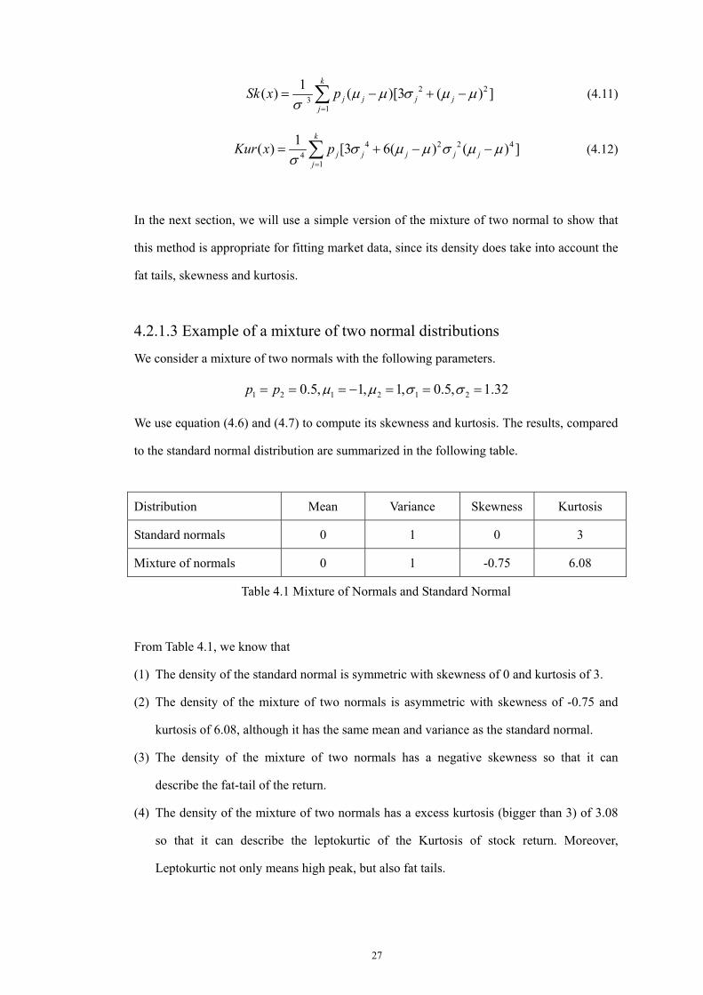
From Table 4.1, we know that

(1) The density of the standard normal is symmetric with skewness of 0 and kurtosis of 3.

(2) The density of the mixture of two normals is asymmetric with skewness of -0.75 and

kurtosis of 6.08, although it has the same mean and variance as the standard normal.

(3) The density of the mixture of two normals has a negative skewness so that it can

describe the fat-tail of the return.

(4) The density of the mixture of two normals has a excess kurtosis (bigger than 3) of 3.08

so that it can describe the leptokurtic of the Kurtosis of stock return. Moreover,

Leptokurtic not only means high peak, but also fat tails.

28

There are three data sets in our research, SSE COMPOSITE, SSE A share, and SSE 30. We

describe the standardized return as follows.

Figure 4.1 Standardized Return of SSE COMPOSITE

Figure 4.2 Standardized Return of SSE A SHARE

29

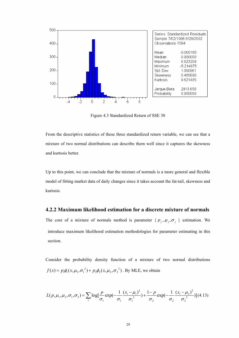
Figure 4.3 Standardized Return of SSE 30

From the descriptive statistics of these three standardized return variable, we can see that a

mixture of two normal distributions can describe them well since it captures the skewness

and kurtosis better.

Up to this point, we can conclude that the mixture of normals is a more general and flexible

model of fitting market data of daily changes since it takes account the fat-tail, skewness and

kurtosis.

4.2.2 Maximum likelihood estimation for a discrete mixture of normals

The core of a mixture of normals method is parameter { jp , ,j jµ σ } estimation. We

introduce maximum likelihood estimation methodologies for parameter estimating in this

section.

Consider the probability density function of a mixture of two normal distributions

2 21 1 1 1 2 2 2 2( ) ( , , ) ( , , )f x p x p xφ µ σ φ µ σ= + . By MLE, we obtain

2 21 2

1 2 1 2 2 21 1 1 2 2 2

( ) ( )1 1 1( , , , , ) log[ exp( ) exp( )]t t

t

x xp pL p µ µµ µ σ σσ σ σ σ σ σ

− −−= − + −∑ (4.13)

30

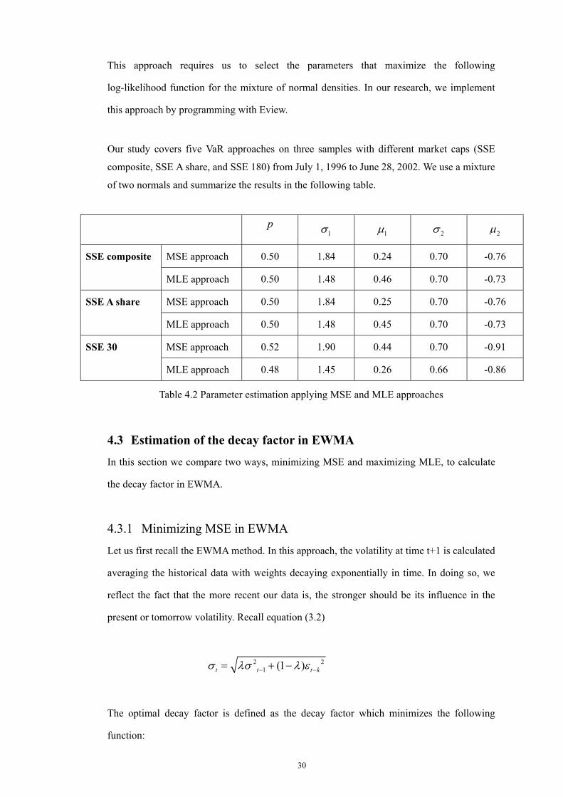
This approach requires us to select the parameters that maximize the following

log-likelihood function for the mixture of normal densities. In our research, we implement

this approach by programming with Eview.

Our study covers five VaR approaches on three samples with different market caps (SSE

composite, SSE A share, and SSE 180) from July 1, 1996 to June 28, 2002. We use a mixture

of two normals and summarize the results in the following table.

p 1σ 1µ 2σ 2µ

MSE approach 0.50 1.84 0.24 0.70 -0.76 SSE composite

MLE approach 0.50 1.48 0.46 0.70 -0.73

MSE approach 0.50 1.84 0.25 0.70 -0.76 SSE A share

MLE approach 0.50 1.48 0.45 0.70 -0.73

MSE approach 0.52 1.90 0.44 0.70 -0.91 SSE 30

MLE approach 0.48 1.45 0.26 0.66 -0.86

Table 4.2 Parameter estimation applying MSE and MLE approaches

4.3 Estimation of the decay factor in EWMA

In this section we compare two ways, minimizing MSE and maximizing MLE, to calculate

the decay factor in EWMA.

4.3.1 Minimizing MSE in EWMA

Let us first recall the EWMA method. In this approach, the volatility at time t+1 is calculated

averaging the historical data with weights decaying exponentially in time. In doing so, we

reflect the fact that the more recent our data is, the stronger should be its influence in the

present or tomorrow volatility. Recall equation (3.2)

2 21 (1 )t t t kσ λσ λ ε− −= + −

The optimal decay factor is defined as the decay factor which minimizes the following

function:

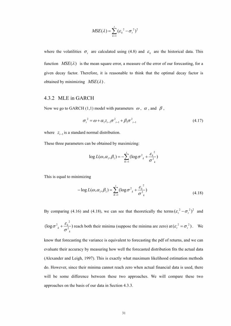
31

2 2 2

1( ) ( )

t

k tk

MSE λ ε σ=

= −∑

where the volatilities tσ are calculated using (4.8) and kε are the historical data. This

function ( )MSE λ is the mean square error, a measure of the error of our forecasting, for a

given decay factor. Therefore, it is reasonable to think that the optimal decay factor is

obtained by minimizing ( )MSE λ .

4.3.2 MLE in GARCH

Now we go to GARCH (1,1) model with parameters ω , α , and β ,

2 2 21 1 1 1 1t t t tzσ ω α σ β σ− − −= + + (4.17)

where 1tz − is a standard normal distribution.

These three parameters can be obtained by maximizing:

22

1 1 21

log ( , , ) (log )t

kk

K k

L εω α β σσ=

= − +∑

This is equal to minimizing

22

1 1 21

log ( , , ) (log )t

kk

K k

L εω α β σσ=

− = +∑ (4.18)

By comparing (4.16) and (4.18), we can see that theoretically the terms 2 2 2( )t tε σ− and

22

2(log )kk

k

εσσ

+ reach both their minima (suppose the minima are zero) at 2 2( )t tε σ= . We

know that forecasting the variance is equivalent to forecasting the pdf of returns, and we can

evaluate their accuracy by measuring how well the forecasted distribution fits the actual data

(Alexander and Leigh, 1997). This is exactly what maximum likelihood estimation methods

do. However, since their minima cannot reach zero when actual financial data is used, there

will be some difference between these two approaches. We will compare these two

approaches on the basis of our data in Section 4.3.3.

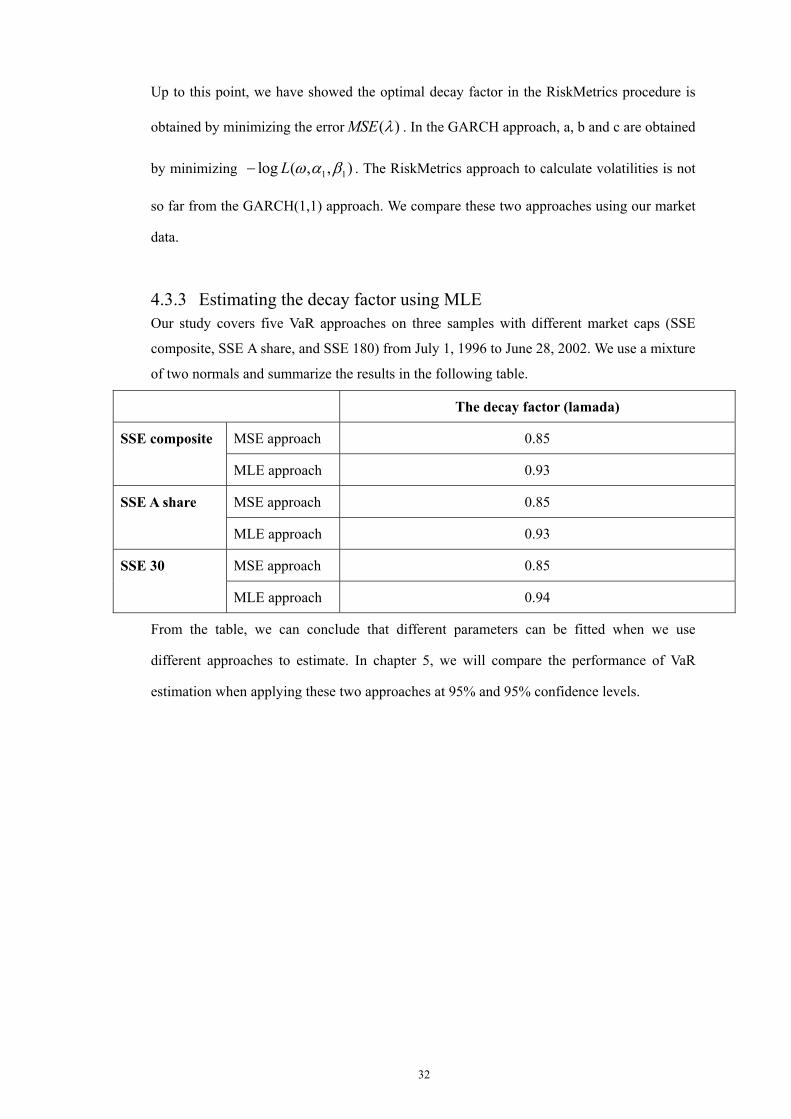
32

Up to this point, we have showed the optimal decay factor in the RiskMetrics procedure is

obtained by minimizing the error ( )MSE λ . In the GARCH approach, a, b and c are obtained

by minimizing 1 1log ( , , )L ω α β− . The RiskMetrics approach to calculate volatilities is not

so far from the GARCH(1,1) approach. We compare these two approaches using our market

data.

4.3.3 Estimating the decay factor using MLE Our study covers five VaR approaches on three samples with different market caps (SSE

composite, SSE A share, and SSE 180) from July 1, 1996 to June 28, 2002. We use a mixture

of two normals and summarize the results in the following table.

The decay factor (lamada)

MSE approach 0.85 SSE composite

MLE approach 0.93

MSE approach 0.85 SSE A share

MLE approach 0.93

MSE approach 0.85 SSE 30

MLE approach 0.94

From the table, we can conclude that different parameters can be fitted when we use

different approaches to estimate. In chapter 5, we will compare the performance of VaR

estimation when applying these two approaches at 95% and 95% confidence levels.

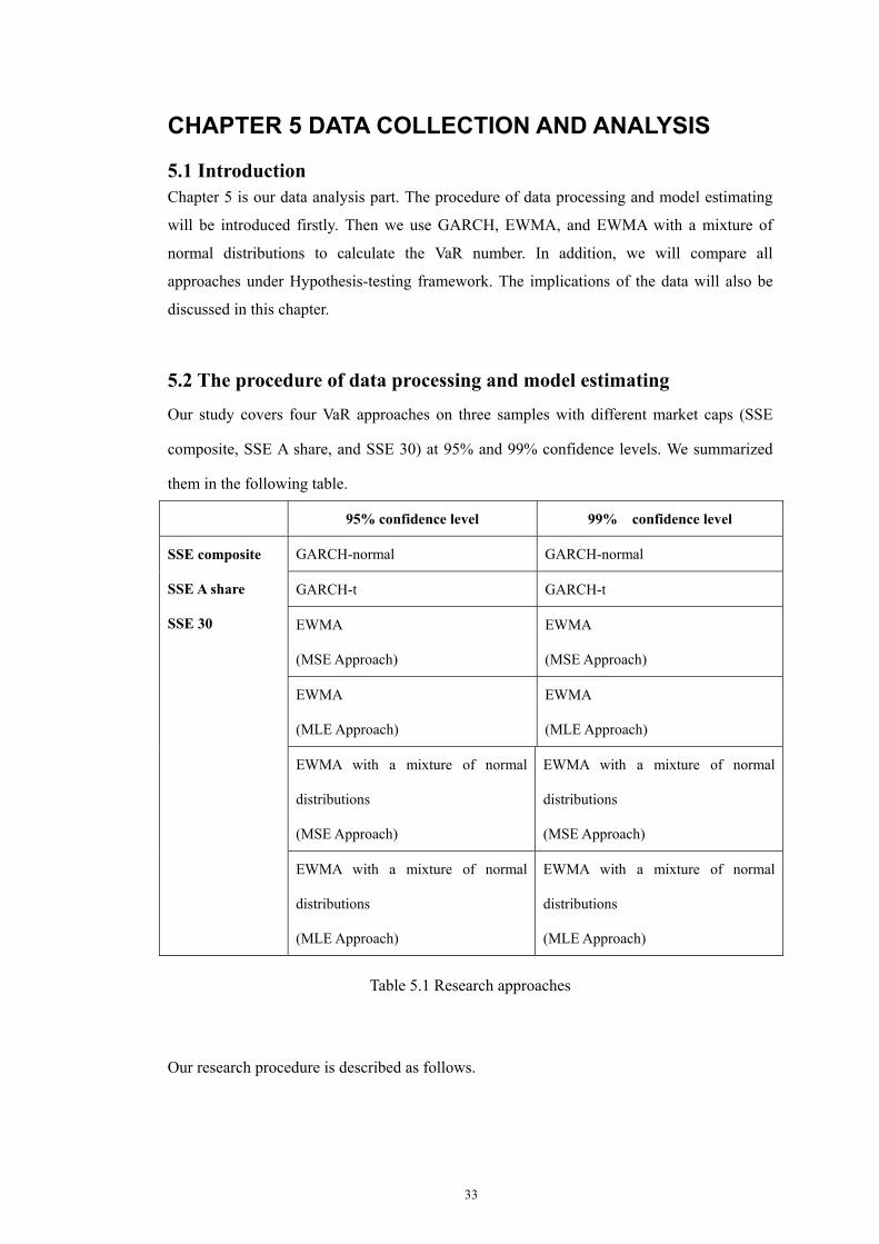
33

CHAPTER 5 DATA COLLECTION AND ANALYSIS

5.1 Introduction Chapter 5 is our data analysis part. The procedure of data processing and model estimating

will be introduced firstly. Then we use GARCH, EWMA, and EWMA with a mixture of

normal distributions to calculate the VaR number. In addition, we will compare all

approaches under Hypothesis-testing framework. The implications of the data will also be

discussed in this chapter.

5.2 The procedure of data processing and model estimating

Our study covers four VaR approaches on three samples with different market caps (SSE

composite, SSE A share, and SSE 30) at 95% and 99% confidence levels. We summarized

them in the following table.

95% confidence level 99% confidence level

GARCH-normal GARCH-normal

GARCH-t GARCH-t

EWMA

(MSE Approach)

EWMA

(MSE Approach)

EWMA

(MLE Approach)

EWMA

(MLE Approach)

EWMA with a mixture of normal

distributions

(MSE Approach)

EWMA with a mixture of normal

distributions

(MSE Approach)

SSE composite

SSE A share

SSE 30

EWMA with a mixture of normal

distributions

(MLE Approach)

EWMA with a mixture of normal

distributions

(MLE Approach)

Table 5.1 Research approaches

Our research procedure is described as follows.

34

GARCH approach

Step 1: Estimate mean equation

Step 2: Estimate variance equation

Step 3: Calculate conditional variance

Step 4: Calculate VaR

Step 5: Hypothesis testing

EWMA approach

Step 1: Calculate the optimal decay factor (lamada) using MLE and MSE

Step 2: Calculate conditional variance

Step 4: Calculate VaR

Step 5: Hypothesis testing

EWMA with a mixture

of normals

Step 1: Estimate parameter using MLE

Step 2: Calculate conditional variance

Step 3: Calculate the quintile for standardized return

Step 4: Calculate VaR

Step 5: Hypothesis testing

Table 5.2 Research procedure

5.3 Data Collection The first question is how many observations should be used. For EWMA, we follow Jorion’s

suggestion to use a wider data window in order to be able to estimate potential movements

accurately and to estimate the variance with precision. In addition, the GARCH structure

requires large numbers of observations to produce reliable estimates. So, we prefer a large

sample in our research.

The next question is which period will be used. Before 1993 the cap of China’s stock market

is very small and the market is very stable. So we will only use data after 1993. Also, since

we need to select three samples SSE 30 which was began on July 1, 1996 and replaced by

SSE 30 180 on June 28, 2002. Therefore, we select July 1, 1996 to June 28, 2002 as our

sample period. The data of SSE composite, SSE A share, and SSE 180 are downloaded from

DATASTREAM.

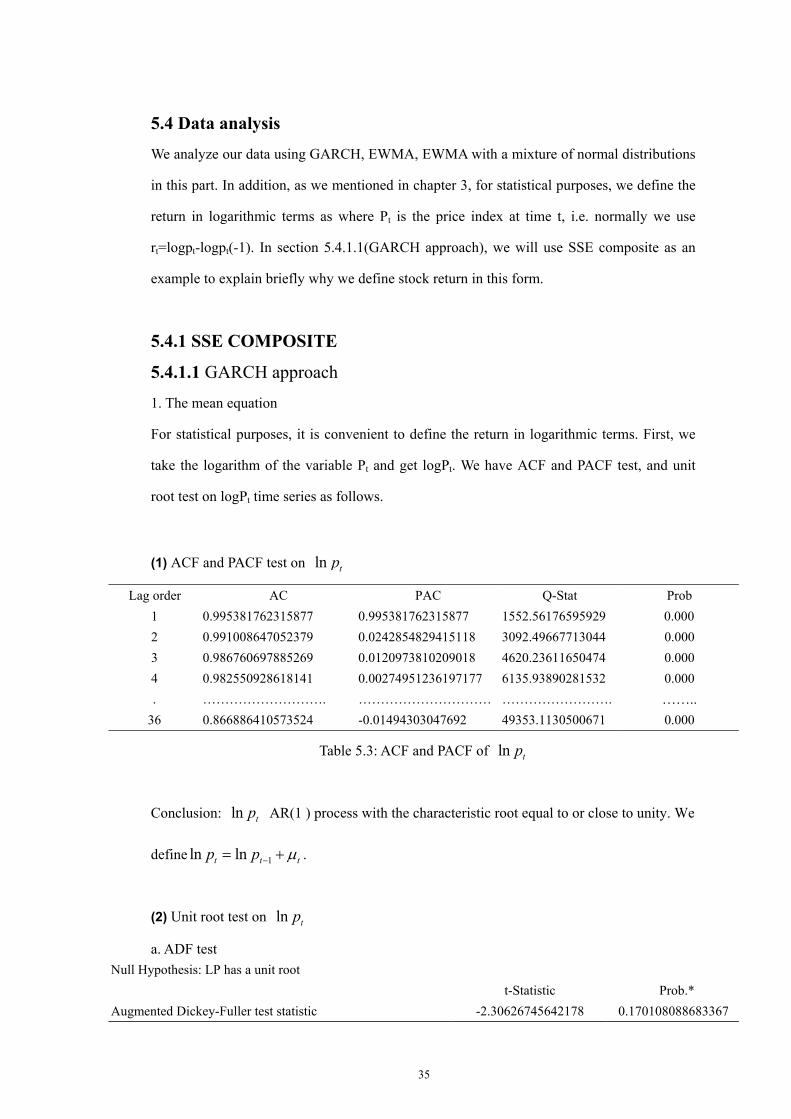
35

5.4 Data analysis

We analyze our data using GARCH, EWMA, EWMA with a mixture of normal distributions

in this part. In addition, as we mentioned in chapter 3, for statistical purposes, we define the

return in logarithmic terms as where Pt is the price index at time t, i.e. normally we use

rt=logpt-logpt(-1). In section 5.4.1.1(GARCH approach), we will use SSE composite as an

example to explain briefly why we define stock return in this form.

5.4.1 SSE COMPOSITE

5.4.1.1 GARCH approach

1. The mean equation

For statistical purposes, it is convenient to define the return in logarithmic terms. First, we

take the logarithm of the variable Pt and get logPt. We have ACF and PACF test, and unit

root test on logPt time series as follows.

(1) ACF and PACF test on ln tp

Lag order AC PAC Q-Stat Prob 1 0.995381762315877 0.995381762315877 1552.56176595929 0.000 2 0.991008647052379 0.0242854829415118 3092.49667713044 0.000 3 0.986760697885269 0.0120973810209018 4620.23611650474 0.000 4 0.982550928618141 0.00274951236197177 6135.93890281532 0.000 . ………………………. ………………………… ……………………. ……..

36 0.866886410573524 -0.01494303047692 49353.1130500671 0.000

Table 5.3: ACF and PACF of ln tp

Conclusion: ln tp AR(1 ) process with the characteristic root equal to or close to unity. We

define 1ln lnt t tp p µ−= + .

(2) Unit root test on ln tp

a. ADF test Null Hypothesis: LP has a unit root

t-Statistic Prob.* Augmented Dickey-Fuller test statistic -2.30626745642178 0.170108088683367

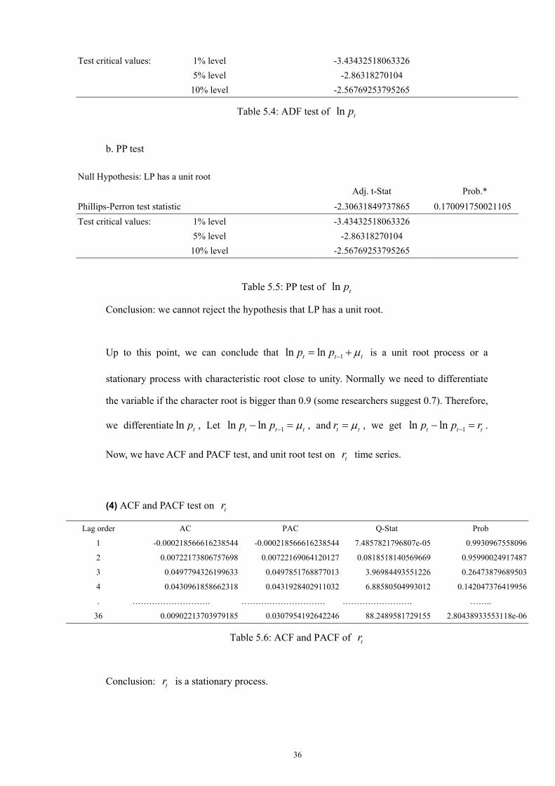
36

Test critical values: 1% level -3.43432518063326 5% level -2.86318270104 10% level -2.56769253795265

Table 5.4: ADF test of ln tp

b. PP test

Table 5.5: PP test of ln tp

Conclusion: we cannot reject the hypothesis that LP has a unit root.

Up to this point, we can conclude that 1ln lnt t tp p µ−= + is a unit root process or a

stationary process with characteristic root close to unity. Normally we need to differentiate

the variable if the character root is bigger than 0.9 (some researchers suggest 0.7). Therefore,

we differentiate ln tp , Let 1ln lnt t tp p µ−− = , and t tr µ= , we get 1ln lnt t tp p r−− = .

Now, we have ACF and PACF test, and unit root test on tr time series.

(4) ACF and PACF test on tr

Lag order AC PAC Q-Stat Prob

1 -0.000218566616238544 -0.000218566616238544 7.4857821796807e-05 0.9930967558096

2 0.00722173806757698 0.00722169064120127 0.0818518140569669 0.95990024917487

3 0.0497794326199633 0.0497851768877013 3.96984493551226 0.26473879689503

4 0.0430961858662318 0.0431928402911032 6.88580504993012 0.142047376419956

. ………………………. ………………………… ……………………. ……..

36 0.00902213703979185 0.0307954192642246 88.2489581729155 2.80438933553118e-06

Table 5.6: ACF and PACF of tr

Conclusion: tr is a stationary process.

Null Hypothesis: LP has a unit root Adj. t-Stat Prob.*

Phillips-Perron test statistic -2.30631849737865 0.170091750021105Test critical values: 1% level -3.43432518063326

5% level -2.86318270104 10% level -2.56769253795265

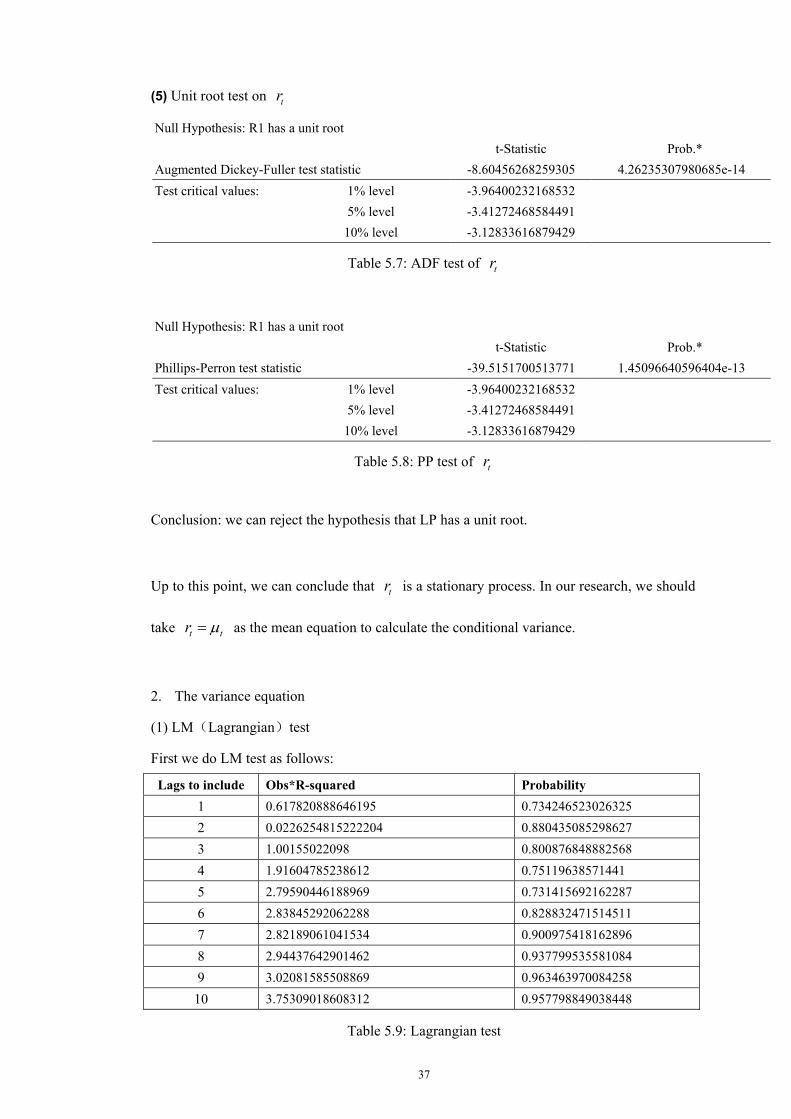
37

(5) Unit root test on tr

Null Hypothesis: R1 has a unit root t-Statistic Prob.*

Augmented Dickey-Fuller test statistic -8.60456268259305 4.26235307980685e-14 Test critical values: 1% level -3.96400232168532

5% level -3.41272468584491 10% level -3.12833616879429

Table 5.7: ADF test of tr

Null Hypothesis: R1 has a unit root t-Statistic Prob.*

Phillips-Perron test statistic -39.5151700513771 1.45096640596404e-13 Test critical values: 1% level -3.96400232168532

5% level -3.41272468584491 10% level -3.12833616879429

Table 5.8: PP test of tr

Conclusion: we can reject the hypothesis that LP has a unit root.

Up to this point, we can conclude that tr is a stationary process. In our research, we should

take t tr µ= as the mean equation to calculate the conditional variance.

2. The variance equation

(1) LM（Lagrangian）test

First we do LM test as follows:

Lags to include Obs*R-squared Probability 1 0.617820888646195 0.734246523026325 2 0.0226254815222204 0.880435085298627 3 1.00155022098 0.800876848882568 4 1.91604785238612 0.75119638571441 5 2.79590446188969 0.731415692162287 6 2.83845292062288 0.828832471514511 7 2.82189061041534 0.900975418162896 8 2.94437642901462 0.937799535581084 9 3.02081585508869 0.963463970084258

10 3.75309018608312 0.957798849038448

Table 5.9: Lagrangian test

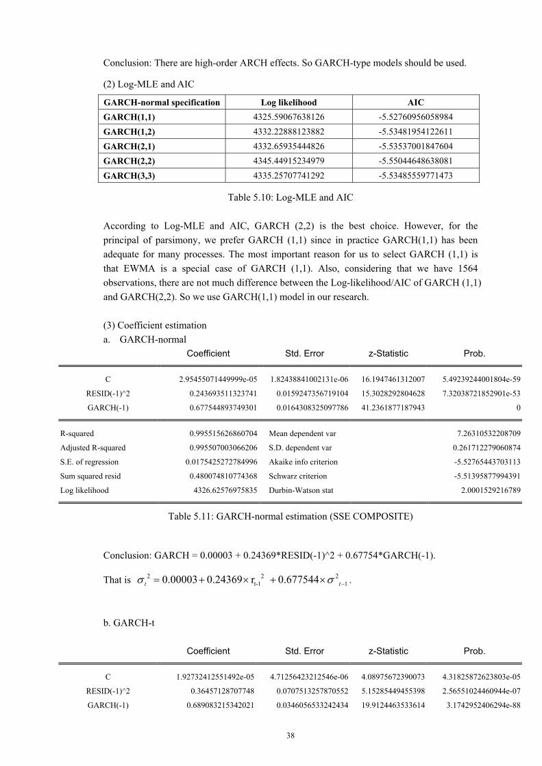
38

Conclusion: There are high-order ARCH effects. So GARCH-type models should be used.

(2) Log-MLE and AIC

GARCH-normal specification Log likelihood AIC GARCH(1,1) 4325.59067638126 -5.52760956058984 GARCH(1,2) 4332.22888123882 -5.53481954122611 GARCH(2,1) 4332.65935444826 -5.53537001847604 GARCH(2,2) 4345.44915234979 -5.55044648638081 GARCH(3,3) 4335.25707741292 -5.53485559771473

Table 5.10: Log-MLE and AIC According to Log-MLE and AIC, GARCH (2,2) is the best choice. However, for the principal of parsimony, we prefer GARCH (1,1) since in practice GARCH(1,1) has been adequate for many processes. The most important reason for us to select GARCH (1,1) is that EWMA is a special case of GARCH (1,1). Also, considering that we have 1564 observations, there are not much difference between the Log-likelihood/AIC of GARCH (1,1) and GARCH(2,2). So we use GARCH(1,1) model in our research. (3) Coefficient estimation a. GARCH-normal

Coefficient Std. Error z-Statistic Prob.

C 2.95455071449999e-05 1.82438841002131e-06 16.1947461312007 5.49239244001804e-59

RESID(-1)^2 0.243693511323741 0.0159247356719104 15.3028292804628 7.32038721852901e-53

GARCH(-1) 0.677544893749301 0.0164308325097786 41.2361877187943 0

R-squared 0.995515626860704 Mean dependent var 7.26310532208709

Adjusted R-squared 0.995507003066206 S.D. dependent var 0.261712279060874

S.E. of regression 0.0175425272784996 Akaike info criterion -5.52765443703113

Sum squared resid 0.480074810774368 Schwarz criterion -5.51395877994391

Log likelihood 4326.62576975835 Durbin-Watson stat 2.0001529216789

Table 5.11: GARCH-normal estimation (SSE COMPOSITE)

Conclusion: GARCH = 0.00003 + 0.24369*RESID(-1)^2 + 0.67754*GARCH(-1).

That is 2 2 2t-1 10.00003 0.24369 r 0.677544t tσ σ −= + × + × .

b. GARCH-t

Coefficient Std. Error z-Statistic Prob.

C 1.92732412551492e-05 4.71256423212546e-06 4.08975672390073 4.31825872623803e-05

RESID(-1)^2 0.36457128707748 0.0707513257870552 5.15285449455398 2.56551024460944e-07

GARCH(-1) 0.689083215342021 0.0346056533242434 19.9124463533614 3.1742952406294e-88

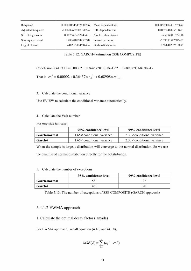
39

R-squared -0.000901515472834236 Mean dependent var 0.000526012431575692

Adjusted R-squared -0.00282632607951294 S.D. dependent var 0.0175246075511683

S.E. of regression 0.0175493552049491 Akaike info criterion -5.7274311329218

Sum squared resid 0.480448594250778 Schwarz criterion -5.71373547583457

Log likelihood 4482.85114594484 Durbin-Watson stat 1.99846237612877

Table 5.12: GARCH-t estimation (SSE COMPOSITE)

Conclusion: GARCH = 0.00002 + 0.36457*RESID(-1)^2 + 0.68908*GARCH(-1).

That is 2 2 2t-1 10.00002 0.36457 r 0.68908t tσ σ −= + × + × .

3. Calculate the conditional variance

Use EVIEW to calculate the conditional variance automatically.

4. Calculate the VaR number

For one-side tail case,

95% confidence level 99% confidence level Garch-normal 1.65×conditional variance 2.33×conditional variance Garch-t 1.65×conditional variance 2.33×conditional variance

When the sample is large, t-distribution will converge to the normal distribution. So we use

the quantile of normal distribution directly for the t-distribution.

5. Calculate the number of exceptions

95% confidence level 99% confidence level Garch-normal 58 22 Garch-t 48 20

Table 5.13: The number of exceptions of SSE COMPOSITE (GARCH approach)

5.4.1.2 EWMA approach

1. Calculate the optimal decay factor (lamada)

For EWMA approach, recall equation (4.16) and (4.18),

2 2

1( ) ( )

t

k tk

MSE λ ε σ=

= −∑

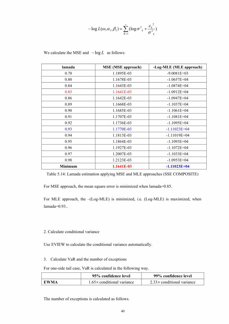
40

22

1 1 21

log ( , , ) (log )t

kk

K k

L εω α β σσ=

− = +∑

We calculate the MSE and log L− as follows:

lamada MSE (MSE approach) -Log-MLE (MLE approach) 0.70 1.1895E-03 -9.0081E+03 0.80 1.1678E-03 -1.0657E+04 0.84 1.1643E-03 -1.0874E+04 0.85 1.1641E-03 -1.0912E+04 0.86 1.1642E-03 -1.0947E+04 0.89 1.1668E-03 -1.1037E+04 0.90 1.1685E-03 -1.1061E+04 0.91 1.1707E-03 -1.1081E+04 0.92 1.1736E-03 -1.1095E+04 0.93 1.1770E-03 -1.11023E+04 0.94 1.1813E-03 -1.11019E+04 0.95 1.1864E-03 -1.1093E+04 0.96 1.1927E-03 -1.1072E+04 0.97 1.2007E-03 -1.1033E+04 0.98 1.2123E-03 -1.0953E+04

Minimum 1.1641E-03 -1.11023E+04

Table 5.14: Lamada estimation applying MSE and MLE approaches (SSE COMPOSITE)

For MSE approach, the mean square error is minimized when lamada=0.85.

For MLE approach, the –(Log-MLE) is minimized, i.e. (Log-MLE) is maximized, when

lamada=0.93..

2. Calculate conditional variance

Use EVIEW to calculate the conditional variance automatically.

3. Calculate VaR and the number of exceptions

For one-side tail case, VaR is calculated in the following way.

95% confidence level 99% confidence level EWMA 1.65×conditional variance 2.33×conditional variance

The number of exceptions is calculated as follows.

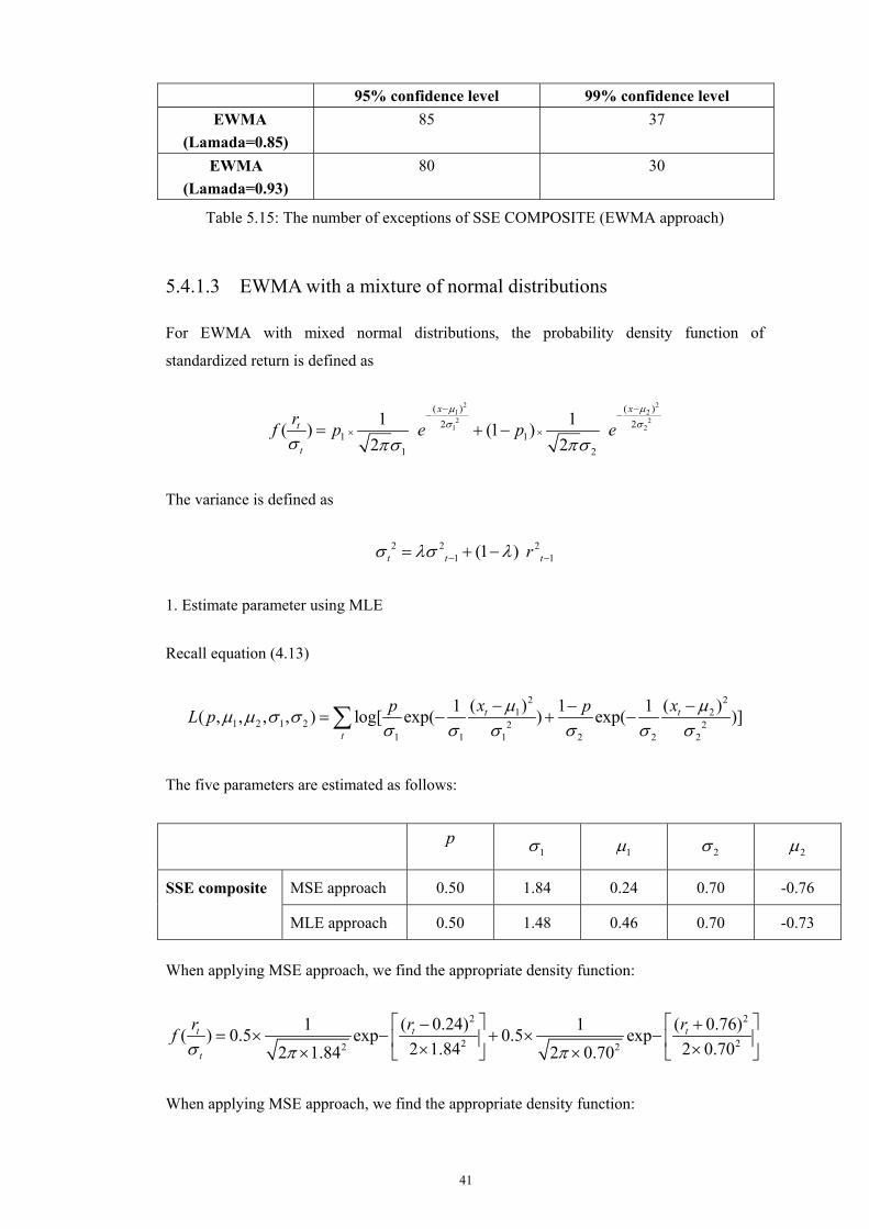
41

95% confidence level 99% confidence level EWMA

(Lamada=0.85) 85 37

EWMA (Lamada=0.93)

80 30

Table 5.15: The number of exceptions of SSE COMPOSITE (EWMA approach)

5.4.1.3 EWMA with a mixture of normal distributions

For EWMA with mixed normal distributions, the probability density function of

standardized return is defined as

2 21 22 2

1 2

( ) ( )2 2

1 11 2

1 1( ) (1 )2 2

x xt

t

rf p e p eµ µσ σ

σ πσ πσ

− −− −

× ×= + −

The variance is defined as

2 2 21 1(1 )t t trσ λσ λ− −= + −

1. Estimate parameter using MLE

Recall equation (4.13)

2 21 2

1 2 1 2 2 21 1 1 2 2 2

( ) ( )1 1 1( , , , , ) log[ exp( ) exp( )]t t

t

x xp pL p µ µµ µ σ σσ σ σ σ σ σ

− −−= − + −∑

The five parameters are estimated as follows:

p 1σ 1µ 2σ 2µ

MSE approach 0.50 1.84 0.24 0.70 -0.76 SSE composite

MLE approach 0.50 1.48 0.46 0.70 -0.73

When applying MSE approach, we find the appropriate density function:

2 2

2 22 2

( 0.24) ( 0.76)1 1( ) 0.5 exp 0.5 exp2 1.84 2 0.702 1.84 2 0.70

t t t

t

r r rfσ π π

− += × − + × − × ×× ×

When applying MSE approach, we find the appropriate density function:

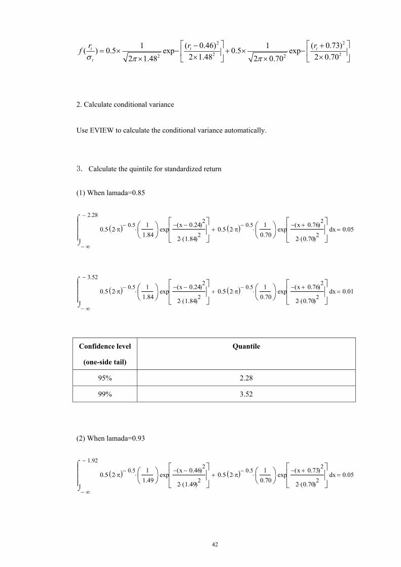
42

2 2

2 22 2

( 0.46) ( 0.73)1 1( ) 0.5 exp 0.5 exp2 1.48 2 0.702 1.48 2 0.70

t t t

t

r r rfσ π π

− += × − + × − × ×× ×

2. Calculate conditional variance

Use EVIEW to calculate the conditional variance automatically.

3. Calculate the quintile for standardized return

(1) When lamada=0.85

∞−

2.28−

x0.5 2 π⋅( ) 0.5−⋅

11.84

⋅ expx 0.24−( )2

−

2 1.84( )2⋅

⋅ 0.5 2 π⋅( ) 0.5−⋅

10.70

⋅ expx 0.76+( )2

−

2 0.70( )2⋅

⋅+

⌠⌡

d 0.05=

∞−

3.52−

x0.5 2 π⋅( ) 0.5−⋅

11.84

⋅ expx 0.24−( )2

−

2 1.84( )2⋅

⋅ 0.5 2 π⋅( ) 0.5−⋅

10.70

⋅ expx 0.76+( )2

−

2 0.70( )2⋅

⋅+

⌠⌡

d 0.01=

Confidence level

(one-side tail)

Quantile

95% 2.28

99% 3.52

(2) When lamada=0.93

∞−

1.92−

x0.5 2 π⋅( ) 0.5−⋅

11.49

⋅ expx 0.46−( )2

−

2 1.49( )2⋅

⋅ 0.5 2 π⋅( ) 0.5−⋅

10.70

⋅ expx 0.73+( )2

−

2 0.70( )2⋅

⋅+

⌠⌡

d 0.05=

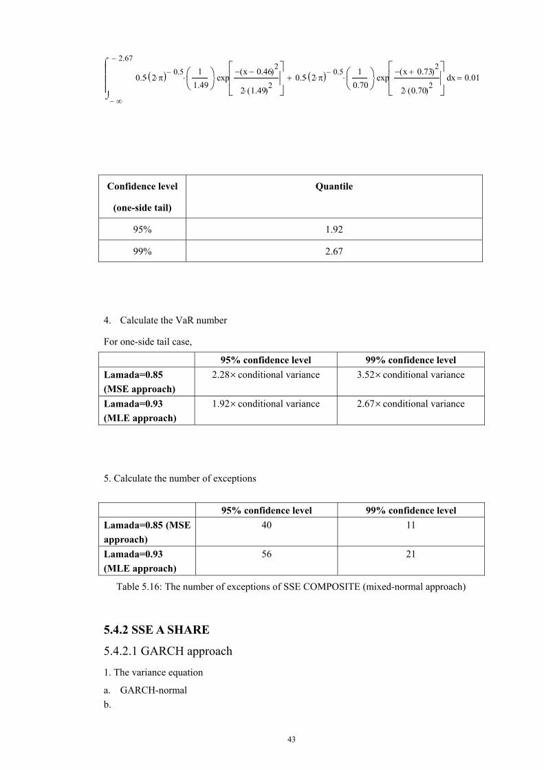
43

∞−

2.67−

x0.5 2 π⋅( ) 0.5−⋅

11.49

⋅ expx 0.46−( )2

−

2 1.49( )2⋅

⋅ 0.5 2 π⋅( ) 0.5−⋅

10.70

⋅ expx 0.73+( )2

−

2 0.70( )2⋅

⋅+

⌠⌡

d 0.01=

Confidence level

(one-side tail)

Quantile

95% 1.92

99% 2.67

4. Calculate the VaR number

For one-side tail case,

95% confidence level 99% confidence level Lamada=0.85 (MSE approach)

2.28×conditional variance 3.52×conditional variance

Lamada=0.93 (MLE approach)

1.92×conditional variance 2.67×conditional variance

5. Calculate the number of exceptions

95% confidence level 99% confidence level Lamada=0.85 (MSE approach)

40 11

Lamada=0.93 (MLE approach)

56 21

Table 5.16: The number of exceptions of SSE COMPOSITE (mixed-normal approach)

5.4.2 SSE A SHARE

5.4.2.1 GARCH approach

1. The variance equation

a. GARCH-normal b.

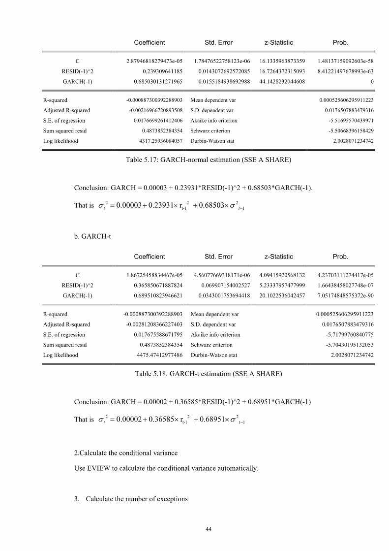
44

Coefficient Std. Error z-Statistic Prob.

C 2.87946818279473e-05 1.78476522758123e-06 16.1335963873359 1.48137159092603e-58

RESID(-1)^2 0.239309641185 0.0143072692572085 16.7264372315093 8.41221497678993e-63

GARCH(-1) 0.685030131271965 0.0155184938692988 44.1428232044608 0

R-squared -0.000887300392288903 Mean dependent var 0.000525606295911223

Adjusted R-squared -0.00216966720893508 S.D. dependent var 0.0176507883479316

S.E. of regression 0.0176699261412406 Akaike info criterion -5.51695570439971

Sum squared resid 0.4873852384354 Schwarz criterion -5.50668396158429

Log likelihood 4317.25936084057 Durbin-Watson stat 2.0028071234742

Table 5.17: GARCH-normal estimation (SSE A SHARE)

Conclusion: GARCH = 0.00003 + 0.23931*RESID(-1)^2 + 0.68503*GARCH(-1).

That is 2 2 2t-1 10.00003 0.23931 r 0.68503t tσ σ −= + × + ×

b. GARCH-t

Coefficient Std. Error z-Statistic Prob.

C 1.86725458834467e-05 4.56077669318171e-06 4.09415920568132 4.23703111274417e-05

RESID(-1)^2 0.365850671887824 0.069907154002527 5.23337957477999 1.66438458027748e-07

GARCH(-1) 0.689510823946621 0.0343001753694418 20.1022536042457 7.05174848575372e-90

R-squared -0.000887300392288903 Mean dependent var 0.000525606295911223

Adjusted R-squared -0.00281208366227403 S.D. dependent var 0.0176507883479316

S.E. of regression 0.017675588671795 Akaike info criterion -5.71799760840775

Sum squared resid 0.4873852384354 Schwarz criterion -5.70430195132053

Log likelihood 4475.47412977486 Durbin-Watson stat 2.0028071234742

Table 5.18: GARCH-t estimation (SSE A SHARE)

Conclusion: GARCH = 0.00002 + 0.36585*RESID(-1)^2 + 0.68951*GARCH(-1)

That is 2 2 2t-1 10.00002 0.36585 r 0.68951t tσ σ −= + × + ×

2.Calculate the conditional variance

Use EVIEW to calculate the conditional variance automatically.

3. Calculate the number of exceptions

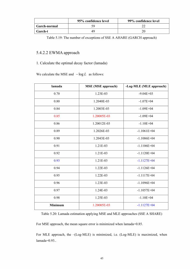
45

95% confidence level 99% confidence level Garch-normal 59 22 Garch-t 49 20

Table 5.19: The number of exceptions of SSE A AHARE (GARCH approach)

5.4.2.2 EWMA approach

1. Calculate the optimal decay factor (lamada)

We calculate the MSE and log L− as follows:

lamada MSE (MSE approach) -Log-MLE (MLE approach)

0.70 1.23E-03 -9.04E+03

0.80 1.2040E-03 -1.07E+04

0.84 1.2003E-03 -1.09E+04

0.85 1.20005E-03 -1.09E+04

0.86 1.20012E-03 -1.10E+04

0.89 1.2026E-03 -1.1061E+04

0.90 1.2043E-03 -1.1086E+04

0.91 1.21E-03 -1.1106E+04

0.92 1.21E-03 -1.1120E+04

0.93 1.21E-03 -1.1127E+04

0.94 1.22E-03 -1.1126E+04

0.95 1.22E-03 -1.1117E+04

0.96 1.23E-03 -1.1096E+04

0.97 1.24E-03 -1.1057E+04

0.98 1.25E-03 -1.10E+04

Minimum 1.20005E-03 -1.1127E+04

Table 5.20: Lamada estimation applying MSE and MLE approaches (SSE A SHARE)

For MSE approach, the mean square error is minimized when lamada=0.85.

For MLE approach, the –(Log-MLE) is minimized, i.e. (Log-MLE) is maximized, when

lamada=0.93..

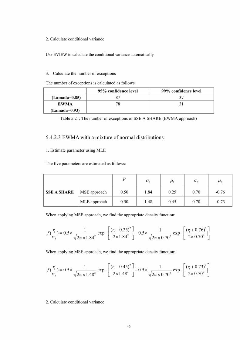
46

2. Calculate conditional variance

Use EVIEW to calculate the conditional variance automatically.

3. Calculate the number of exceptions

The number of exceptions is calculated as follows.

95% confidence level 99% confidence level (Lamada=0.85) 87 37

EWMA (Lamada=0.93)

78 31

Table 5.21: The number of exceptions of SSE A SHARE (EWMA approach)

5.4.2.3 EWMA with a mixture of normal distributions

1. Estimate parameter using MLE

The five parameters are estimated as follows:

p 1σ 1µ 2σ 2µ

MSE approach 0.50 1.84 0.25 0.70 -0.76 SSE A SHARE

MLE approach 0.50 1.48 0.45 0.70 -0.73

When applying MSE approach, we find the appropriate density function:

2 2

2 22 2

( 0.25) ( 0.76)1 1( ) 0.5 exp 0.5 exp2 1.84 2 0.702 1.84 2 0.70

t t t

t

r r rfσ π π

− += × − + × − × ×× ×

When applying MSE approach, we find the appropriate density function:

2 2

2 22 2

( 0.45) ( 0.73)1 1( ) 0.5 exp 0.5 exp2 1.48 2 0.702 1.48 2 0.70

t t t

t

r r rfσ π π

− += × − + × − × ×× ×

2. Calculate conditional variance

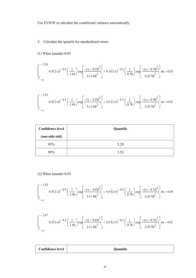
47

Use EVIEW to calculate the conditional variance automatically.

3. Calculate the quintile for standardized return

(1) When lamada=0.85

∞−

2.28−

x0.5 2 π⋅( ) 0.5−⋅

11.84

⋅ expx 0.25−( )2

−

2 1.84( )2⋅

⋅ 0.5 2 π⋅( ) 0.5−⋅

10.70

⋅ expx 0.76+( )2

−

2 0.70( )2⋅

⋅+

⌠⌡

d 0.05=

∞−

3.52−

x0.5 2 π⋅( ) 0.5−⋅

11.84

⋅ expx 0.25−( )2

−

2 1.84( )2⋅

⋅ 0.5 2 π⋅( ) 0.5−⋅

10.70

⋅ expx 0.76+( )2

−

2 0.70( )2⋅

⋅+

⌠⌡

d 0.01=

Confidence level

(one-side tail)

Quantile

95% 2.28

99% 3.52

(2) When lamada=0.93

∞−

1.92−

x0.5 2 π⋅( ) 0.5−⋅

11.48

⋅ expx 0.45−( )2

−

2 1.48( )2⋅

⋅ 0.5 2 π⋅( ) 0.5−⋅

10.70

⋅ expx 0.73+( )2

−

2 0.70( )2⋅

⋅+

⌠⌡

d 0.05=

∞−

2.67−

x0.5 2 π⋅( ) 0.5−⋅

11.48

⋅ expx 0.45−( )2

−

2 1.48( )2⋅

⋅ 0.5 2 π⋅( ) 0.5−⋅

10.70

⋅ expx 0.73+( )2

−

2 0.70( )2⋅

⋅+

⌠⌡

d 0.01=

Confidence level Quantile

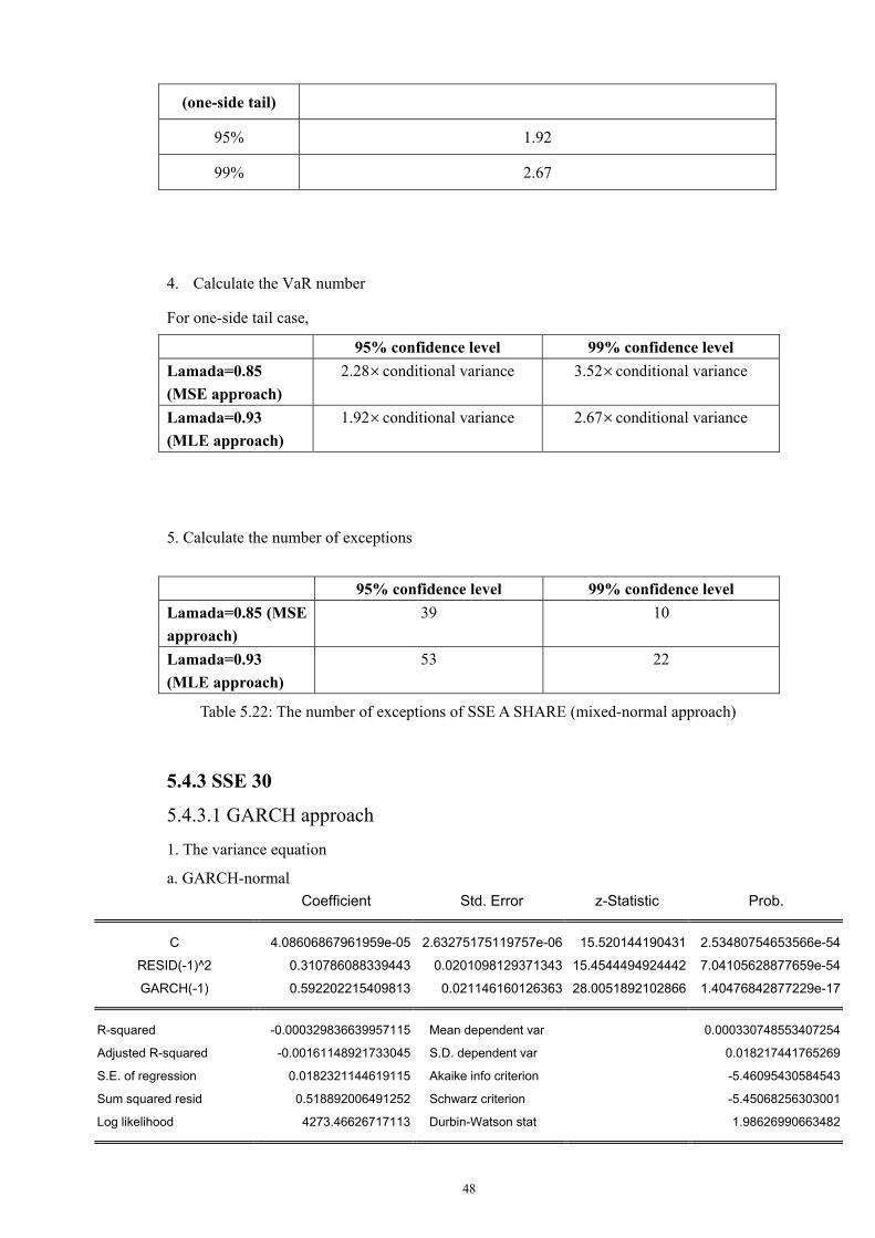
48

(one-side tail)

95% 1.92

99% 2.67

4. Calculate the VaR number

For one-side tail case,

95% confidence level 99% confidence level Lamada=0.85 (MSE approach)

2.28×conditional variance 3.52×conditional variance

Lamada=0.93 (MLE approach)

1.92×conditional variance 2.67×conditional variance

5. Calculate the number of exceptions

95% confidence level 99% confidence level Lamada=0.85 (MSE approach)

39 10

Lamada=0.93 (MLE approach)

53 22

Table 5.22: The number of exceptions of SSE A SHARE (mixed-normal approach)

5.4.3 SSE 30

5.4.3.1 GARCH approach

1. The variance equation

a. GARCH-normal Coefficient Std. Error z-Statistic Prob.

C 4.08606867961959e-05 2.63275175119757e-06 15.520144190431 2.53480754653566e-54

RESID(-1)^2 0.310786088339443 0.0201098129371343 15.4544494924442 7.04105628877659e-54

GARCH(-1) 0.592202215409813 0.021146160126363 28.0051892102866 1.40476842877229e-17

R-squared -0.000329836639957115 Mean dependent var 0.000330748553407254

Adjusted R-squared -0.00161148921733045 S.D. dependent var 0.018217441765269

S.E. of regression 0.0182321144619115 Akaike info criterion -5.46095430584543

Sum squared resid 0.518892006491252 Schwarz criterion -5.45068256303001

Log likelihood 4273.46626717113 Durbin-Watson stat 1.98626990663482

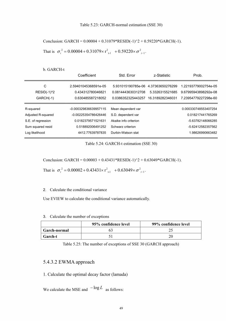
49

Table 5.23: GARCH-normal estimation (SSE 30)

Conclusion: GARCH = 0.00004 + 0.31079*RESID(-1)^2 + 0.59220*GARCH(-1).

That is 2 2 2t-1 10.00004 0.31079 r 0.59220t tσ σ −= + × + × .

b. GARCH-t Coefficient Std. Error z-Statistic Prob.

C 2.59401045368591e-05 5.931015190785e-06 4.37363650276299 1.22193779002754e-05

RESID(-1)^2 0.434312780046821 0.0814443630312708 5.3326315521685 9.67995943898292e-08

GARCH(-1) 0.630485587218052 0.0386352325443257 16.3189282346031 7.23954779227298e-60

R-squared -0.000329836639957115 Mean dependent var 0.000330748553407254

Adjusted R-squared -0.00225354786426446 S.D. dependent var 0.018217441765269

S.E. of regression 0.0182379571521631 Akaike info criterion -5.63782148066285

Sum squared resid 0.518892006491252 Schwarz criterion -5.62412582357562

Log likelihood 4412.77639787835 Durbin-Watson stat 1.98626990663482

Table 5.24: GARCH-t estimation (SSE 30)

Conclusion: GARCH = 0.00003 + 0.43431*RESID(-1)^2 + 0.63049*GARCH(-1).

That is 2 2 2t-1 10.00002 0.43431 r 0.63049t tσ σ −= + × + × .

2. Calculate the conditional variance

Use EVIEW to calculate the conditional variance automatically.

3. Calculate the number of exceptions

95% confidence level 99% confidence level Garch-normal 63 25 Garch-t 51 20

Table 5.25: The number of exceptions of SSE 30 (GARCH approach)

5.4.3.2 EWMA approach

1. Calculate the optimal decay factor (lamada)

We calculate the MSE and log L− as follows:

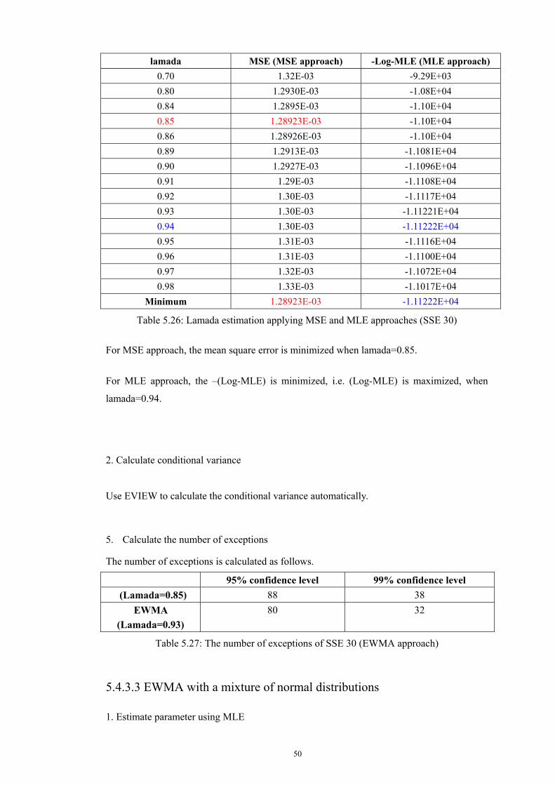
50

lamada MSE (MSE approach) -Log-MLE (MLE approach) 0.70 1.32E-03 -9.29E+03 0.80 1.2930E-03 -1.08E+04 0.84 1.2895E-03 -1.10E+04 0.85 1.28923E-03 -1.10E+04 0.86 1.28926E-03 -1.10E+04 0.89 1.2913E-03 -1.1081E+04 0.90 1.2927E-03 -1.1096E+04 0.91 1.29E-03 -1.1108E+04 0.92 1.30E-03 -1.1117E+04 0.93 1.30E-03 -1.11221E+04 0.94 1.30E-03 -1.11222E+04 0.95 1.31E-03 -1.1116E+04 0.96 1.31E-03 -1.1100E+04 0.97 1.32E-03 -1.1072E+04 0.98 1.33E-03 -1.1017E+04

Minimum 1.28923E-03 -1.11222E+04

Table 5.26: Lamada estimation applying MSE and MLE approaches (SSE 30)

For MSE approach, the mean square error is minimized when lamada=0.85.

For MLE approach, the –(Log-MLE) is minimized, i.e. (Log-MLE) is maximized, when

lamada=0.94.

2. Calculate conditional variance

Use EVIEW to calculate the conditional variance automatically.

5. Calculate the number of exceptions

The number of exceptions is calculated as follows.

95% confidence level 99% confidence level (Lamada=0.85) 88 38

EWMA (Lamada=0.93)

80 32

Table 5.27: The number of exceptions of SSE 30 (EWMA approach)

5.4.3.3 EWMA with a mixture of normal distributions

1. Estimate parameter using MLE

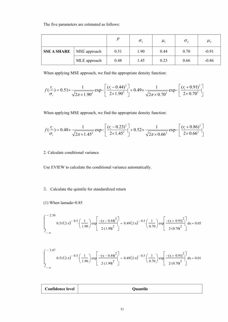
51

The five parameters are estimated as follows:

p 1σ 1µ 2σ 2µ

MSE approach 0.51 1.90 0.44 0.70 -0.91 SSE A SHARE

MLE approach 0.48 1.45 0.23 0.66 -0.86

When applying MSE approach, we find the appropriate density function:

2 2

2 22 2

( 0.44) ( 0.91)1 1( ) 0.51 exp 0.49 exp2 1.90 2 0.702 1.90 2 0.70

t t t

t

r r rfσ π π

− += × − + × − × ×× ×

When applying MSE approach, we find the appropriate density function:

2 2

2 22 2

( 0.23) ( 0.86)1 1( ) 0.48 exp 0.52 exp2 1.45 2 0.662 1.45 2 0.66

t t t

t

r r rfσ π π

− += × − + × − × ×× ×

2. Calculate conditional variance

Use EVIEW to calculate the conditional variance automatically.

3. Calculate the quintile for standardized return

(1) When lamada=0.85

∞−

2.30−

x0.51 2 π⋅( ) 0.5−⋅

11.90

⋅ expx 0.44−( )2

−

2 1.90( )2⋅

⋅ 0.49 2 π⋅( ) 0.5−⋅

10.70

⋅ expx 0.91+( )2

−

2 0.70( )2⋅

⋅+

⌠⌡

d 0.05=

∞−

3.47−

x0.51 2 π⋅( ) 0.5−⋅

11.90

⋅ expx 0.44−( )2

−

2 1.90( )2⋅

⋅ 0.49 2 π⋅( ) 0.5−⋅

10.70

⋅ expx 0.91+( )2

−

2 0.70( )2⋅

⋅+

⌠⌡

d 0.01=

Confidence level Quantile

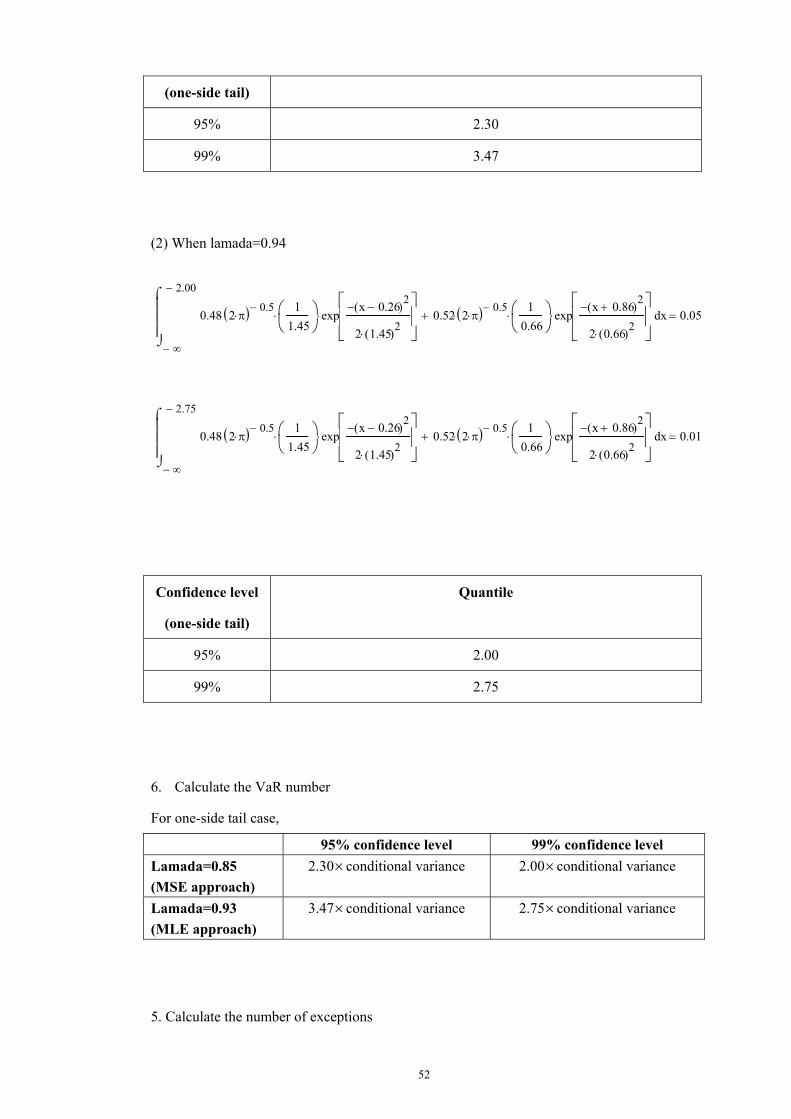
52

(one-side tail)

95% 2.30

99% 3.47

(2) When lamada=0.94

∞−

2.00−

x0.48 2 π⋅( ) 0.5−⋅

11.45

⋅ expx 0.26−( )2

−

2 1.45( )2⋅

⋅ 0.52 2 π⋅( ) 0.5−⋅

10.66

⋅ expx 0.86+( )2

−

2 0.66( )2⋅

⋅+

⌠⌡

d 0.05=

∞−

2.75−

x0.48 2 π⋅( ) 0.5−⋅

11.45

⋅ expx 0.26−( )2

−

2 1.45( )2⋅

⋅ 0.52 2 π⋅( ) 0.5−⋅

10.66

⋅ expx 0.86+( )2

−

2 0.66( )2⋅

⋅+

⌠⌡

d 0.01=

Confidence level

(one-side tail)

Quantile

95% 2.00

99% 2.75

6. Calculate the VaR number

For one-side tail case,

95% confidence level 99% confidence level Lamada=0.85 (MSE approach)

2.30×conditional variance 2.00×conditional variance

Lamada=0.93 (MLE approach)

3.47×conditional variance 2.75×conditional variance

5. Calculate the number of exceptions

53

95% confidence level 99% confidence level Lamada=0.85 (MSE approach)

48 17

Lamada=0.93 (MLE approach)

46 19

Table 5.28: The number of exceptions of SSE 30 (mixed-normal approach)

5.5 Hypothesis-testing

1. Calculate the acceptable range

We have introduced the hypothesis-testing technique proposed by Kupiec (1995) in chapter

2. To illustrate the procedure of decision making, suppose following conditions are given:

Number of exceptions: N Total observations: T

VaR number: VaR VaR confidence level: c

Test confidence level: p

The actual daily loss exceeds VaR or not is a sequence of success or failure with probability

1−c, thus assuming all the observations are independent, this is Bernoulli process, and

follows a binomial distribution. The pdf for this binomial distribution is given by

( ) (1 )N T NTf x C C

N−

= −

, for N=0,1,2,……

Note that for a binomial distribution, Expectation(x) =T (1−c) and Variance(x) =Tc(1−c) .

If the sample size T is large enough, we can apply the central limit theorem, and

approximate the binomial distribution by a normal distribution.

Let(1 )

(1 )N u N T CZ

TC Cσ− − −

= =−

, then by central limit theorem, Z follows a standard normal

distribution N(0, 1). Therefore, given a test confidence level p , Then the range for N can

be calculated as

1 1( ) (1 ) (1 ) ( ) (1 ) (1 )p TC C T C N p TC C T C− −−Φ − + − ≤ ≤ Φ − + −

Where 1( )p−Φ is the quantile of Z .

If the number of exceptions N is within the range, we accept the model, and if N is out of the

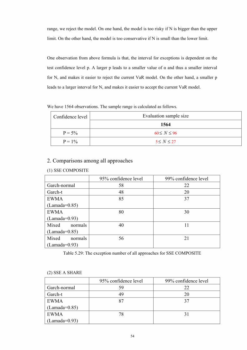
54

range, we reject the model. On one hand, the model is too risky if N is bigger than the upper

limit. On the other hand, the model is too conservative if N is small than the lower limit.

One observation from above formula is that, the interval for exceptions is dependent on the

test confidence level p. A larger p leads to a smaller value of α and thus a smaller interval

for N, and makes it easier to reject the current VaR model. On the other hand, a smaller p

leads to a larger interval for N, and makes it easier to accept the current VaR model.

We have 1564 observations. The sample range is calculated as follows.

Evaluation sample size Confidence level 1564

P = 5% 60 ≤≤ N 96

P = 1% 5 ≤≤ N 27

2. Comparisons among all approaches

(1) SSE COMPOSITE 95% confidence level 99% confidence level Garch-normal 58 22 Garch-t 48 20 EWMA (Lamada=0.85)

85 37

EWMA (Lamada=0.93)

80 30

Mixed normals (Lamada=0.85)

40 11

Mixed normals (Lamada=0.93)

56 21

Table 5.29: The exception number of all approaches for SSE COMPOSITE

(2) SSE A SHARE

95% confidence level 99% confidence level Garch-normal 59 22 Garch-t 49 20 EWMA (Lamada=0.85)

87 37

EWMA (Lamada=0.93)

78 31

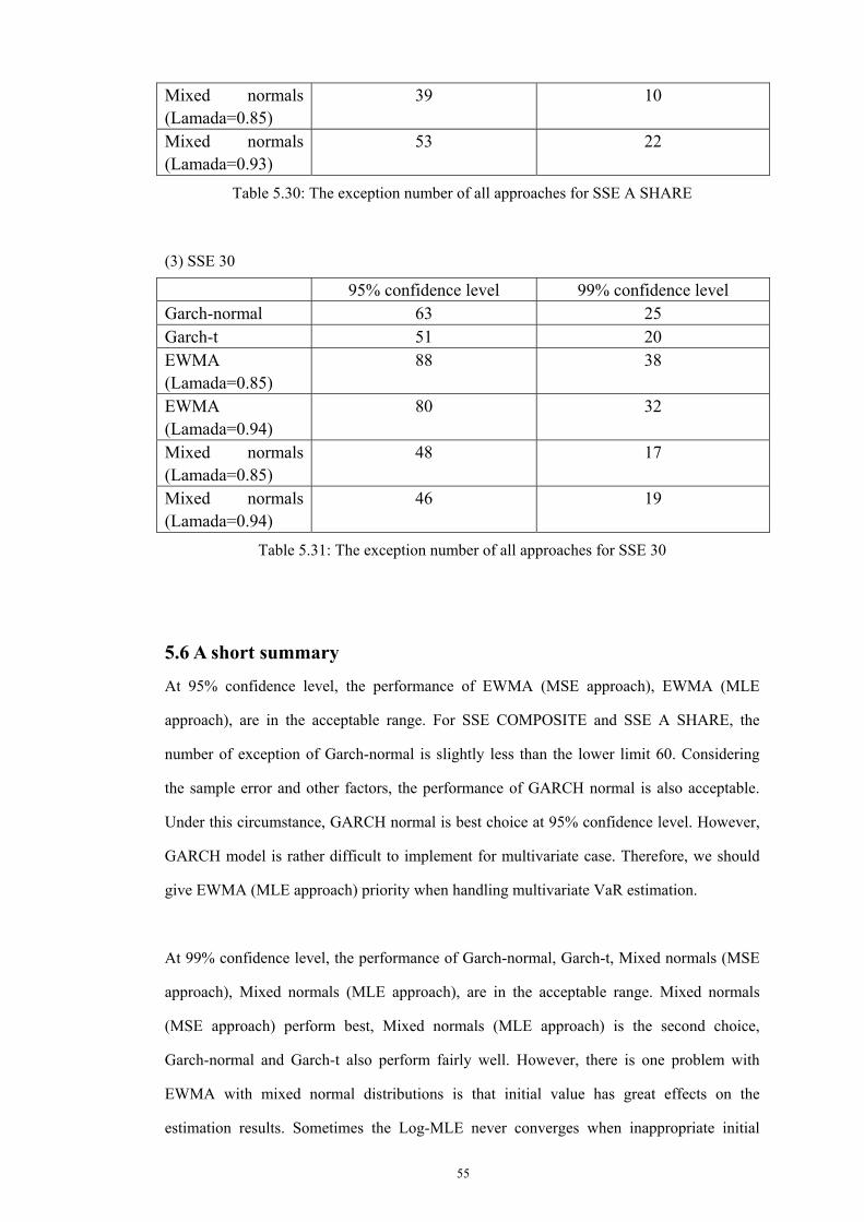
55

Mixed normals (Lamada=0.85)

39 10

Mixed normals (Lamada=0.93)

53 22

Table 5.30: The exception number of all approaches for SSE A SHARE

(3) SSE 30

95% confidence level 99% confidence level Garch-normal 63 25 Garch-t 51 20 EWMA (Lamada=0.85)

88 38

EWMA (Lamada=0.94)

80 32

Mixed normals (Lamada=0.85)

48 17

Mixed normals (Lamada=0.94)

46 19

Table 5.31: The exception number of all approaches for SSE 30

5.6 A short summary

At 95% confidence level, the performance of EWMA (MSE approach), EWMA (MLE

approach), are in the acceptable range. For SSE COMPOSITE and SSE A SHARE, the

number of exception of Garch-normal is slightly less than the lower limit 60. Considering

the sample error and other factors, the performance of GARCH normal is also acceptable.

Under this circumstance, GARCH normal is best choice at 95% confidence level. However,

GARCH model is rather difficult to implement for multivariate case. Therefore, we should

give EWMA (MLE approach) priority when handling multivariate VaR estimation.

At 99% confidence level, the performance of Garch-normal, Garch-t, Mixed normals (MSE

approach), Mixed normals (MLE approach), are in the acceptable range. Mixed normals

(MSE approach) perform best, Mixed normals (MLE approach) is the second choice,

Garch-normal and Garch-t also perform fairly well. However, there is one problem with

EWMA with mixed normal distributions is that initial value has great effects on the

estimation results. Sometimes the Log-MLE never converges when inappropriate initial

56

value is used. So it is more arbitrary than other methods. For practical use (asset manager

without much experience in this field), GARCH-t is a better choice at 99% confidence level.)

However, Mixed normals (MSE approach), Mixed normals (MLE approach) should be used

for multivariate case.

57

CHAPTER 6 CONCLUSION 6.1 Introduction “Which method (VaR methods using RiskMetrics, GARCH-typed models, and EWMA with

a mixture of normal distributions) is better as a reliable and stable risk measurement tool for

Chinese stock markets and an appropriate VaR method for Chinese asset managers to

supervise the portfolio risk and quantify potential losses?” Based on the analysis in prior

chapters, we draw a conclusion on this question. The contribution, limitation and future

research are discussed in this chapter.

6.2 Contribution of the Study There are mainly four contributions of this study. First, there is relatively few researches

regarding VaR in Chinese financial markets. Moreover, we obtain the decay factor both by

MSE approach and MLE approach. And, we compare these two approaches using the same

data set.

Second, we employ EWMA with a mixture of normal distributions and make comparisons

with GARCH-type models. We find mixed state distribution approach is better than GARCH

at 99% confidence level, and GARCH performs better at 95% confidence level.

Third, we develop a clear procedure to determine which GARCH specification is most

appropriate. We first work only on mean equation and ignore heteroscedasticity, and we

proceed to work with the GARCH part based on the "optimal" specification of mean

equation. In this thesis, we choose GARCH (1, 1) specification as our favorite specification

for conditional variance models under the consideration of the principle of parsimony.

Finally, the empirical analysis is performed on different market caps in order to compare the

performance of all the approaches in our research.

6.3 Conclusion At 95% confidence level, the performance of EWMA (MSE approach), EWMA (MLE

approach), and Garch-normal are acceptable. GARCH normal performs best. At 99%

confidence level, Garch-normal, Garch-t, Mixed normals (MSE approach), Mixed normals

(MLE approach) perform fairly well. Mixed normals (MSE approach) is best, the

performance of Mixed normals (MLE approach), Garch-normal and Garch-t are also

acceptable.

58

For unitivariate case our conclusion is

1. GARCH-normal is superior to Riskmetrics approach at both 95% and 99% confidence

levels.

2. GARCH-t is much more conservative than GARCH-normal for VaR estimationat 95%

confidence level. So it is not an appropriate approach at 95% confidence level.

3. EWMA with mixed normal distributions is superior to RiskMetrics approach at 99%

confidence level. But it is too conservative at 95% confidence level.

4. When EWMA with mixed normal distributions compares with GARCH-type, the former

performs better at 99% confidence level. But it is too conservative at 95% confidence level.

So for 95% confidence level, GARCH-normal is a fairly good choice.

6.4 Limitations and Further Research There are limitations in this research and more efforts are needed for further research.

First, the data collected from Chinese financial markets have regional limitations. It may not

be applicable to other time periods and other developing countries. Considering we use a

wider data window which is able to estimate potential movements accurately and to estimate

the variance with precision, we assume the result could be applicable to other time periods of

China’s financial markets; however, more tests should be conducted to get a confirmed

conclusion. As for the other developing countries, the generalization of this study needs more

tests to get a cautious conclusion.

Second, some of the factors have not be tested and explored in this study. Therefore, our

conclusion is only applicable to univariate portfolio. For multivariate case, we should note

that GARCH is hard to use. So the conclusion might change. For example, at 95%

confidence level, GARCH normal is best choice for univariate case. However, we should

give EWMA (MLE approach) priority when handling multivariate VaR estimation. At 99%

confidence level, Mixed normals perform best. However, the Log-MLE never converges

when inappropriate initial value is used. So for practical use, GARCH-t is a better choice at

99% confidence level. However, Mixed normals (MSE approach), Mixed normals (MLE

approach) should be used for multivariate case.

Third, VaR itself, recently, has been criticized as a measure of market risk on two grounds.

First，it is showed that VaR is not necessarily sub-additive, e.g. VaR of a portfolio with two

instruments maybe greater than the sum of individual VaRs of these two instruments and

therefore managing risk by VaR may fail to stimulate diversification. Moreover, VaR does

not give any indication about the size of the potential loss given that the loss exceeds VaR.

In order to remedy the effects of these shortcomings, the Expected Shortfall risk measure has

59

been introduced recently, which is the expected value of the losses conditioned that a VaR

violation has occurred. Some researches substantiated that the proposed procedure generates

losses that are lower than those of the VaR-based risk management techniques. So we should

be cautious when applying VaR to estimate and control risk.

Moreover, in this thesis, we assume that market is efficient. Actually this is not the case for

Chinese stock market. In future research, we can differentiate the market condition into

volatile and non-volatile conditions (using the T-test and the Mann-Whitney U-test) to see

how different VaR model works. For example, in order to see if the results remain the same

for various market conditions, the total data sample can be divided into two sub-samples:

one containing volatility figures greater than or equal to 2% (volatile); and the other

containing volatility figures less than 2% (non-volatile). The same analysis for total sample

could be repeated on the volatile sub-sample and the non-volatile sub-sample. Intuitively, for

EWMA, there might be different lamadas for different market conditions. GARCH model

should perform better than EWMA since it can captures the volatility well.

In addition, there are two lamadas we calculated using MSE and MLE respectively. The

results are quite different for different lamadas. J.P.Morgan recommends lamada by MSE.

Admittedly it is easily to calculate. For estimation, MLE should be more efficient than MSE.

However, it is still uncertain which lamada should be used under each circumstance. In this

thesis, we compare their performances in sample at different significant levels. We should

notice that the comparisons are only based on empirical results. In future research, we can

develop it further in two aspects: (1) find theoretic foundation of these two approaches’

differences and analyze which approach should be more appropriate; (2) apply these two

lamadas to do out-of-sample forecast to determine which one is good for forecasting.

60

BIBLIOGRAPHY

Aczel, D. Amir (1993), Complete Business Statistics. IRWIN.

Aggarwal, R., Inclan, C., Leal, R., 1999, “Volatility in Emerging Stock Markets”, Journal of Financial and Quantitative Analysis 34, 33-55.

Angelidis, T.; Benos, A.; and Degiannakis, S. 2004. The Use of GARCH Models in VaR Estimation. Statistical Methodology.

Bali, T. G., and Theodossiou, P. 2004. A Conditional-SGT-VaR Approach with Alternative GARCH Models. Annals of Operations Research.

Basle Committee on Banking Supervision, 1996, Amendment to the capital accord to incorporate market risks, January.

Barone-Adesi, G.; Giannopoulos, K.; and Vosper, L. 1999. VaR without correlations for nonlinear Portfolios. Journal of Futures Markets 19: 583-602.

Barone-Adesi, G., and Giannopoulos, K. 2001. Non-parametric VaR techniques. Myths and realities. Economic Notes by Banca Monte dei Paschi di Siena SpA 30: 167-181.

Bekaert, G., Erb, C., Campbell, R.H., Viskanta, T.E., 1998, “Distributional Characteristics of Emerging Market Returnas and Asset Allocation”, The Journal of Portfolio Management 24, 102-116.

Bekaert, G., Harvey, C.R., 1997, “Emerging Equity Market Volatility”, Journal of Financial Economics 43, 29-77.

Billio, M. and Pelizzon, L. 2000. Value-at-Risk: A multivariate switching regime approach. Journal of Empirical Finace 7: 531-554.

Bollerslev, T. 1986. A conditional heteroscedastic time series model for speculative prices and rates of return, Review of Economics and Statistics 69: 542-547.

Brooks, C., and Persand, G. 2003. The effect of asymmetries on stock index return Value-at-Risk estimates. The Journal of Risk Finance (Winter): 29-42.

Danielsson, Jon (1998-1999), “Class notes Corporate Finance & Financial Markets”. London School of Economics.

Danielsson, Jon & de Vries, G., Casper (1997), “Value-at-Risk and Extreme Returns”. London School of Economics, Financial Market Group Discussion Paper, No. 273, 1997.

Danielsson, Jon, & de Vries, G., Casper (1997), “Beyond the Sample: Extreme Quantile and Probability Estimation”. http://www.hag.hi.is/~jond/research/.

Dannielsson, J. 2002. The emperor has no clothes: Limits to risk modelling. Journal of Banking& Finance 26: 1273-1296.

Dowd, Kevin (1999), “A Value-at-Risk Approach to Risk-Return Analysis”. The Journal of Portfolio Management, Summer 1999.

61

Du, Haitao, 2000, The application of VaR in security risk management. Security introductory paper 8.

Du, Haitao, 2000, The application of VaR in security risk management. http//:www.drcnet.com.cn.

Engle, R.F. 1982. Autoregressive conditional heteroskedasticity with estimates of the variance of U.K. inflation. Econometrica 50: 987-1008.

Erb, C.B., Harvey, C.R., Viskanta, T.E., 1996, “Expected Returns and Volatility in 135 Countries”, The Journal of Portfolio Management , 46-58.

Frey, R. and Michaud, P. 1997. The effect of garch-type volatilities on prices and payoff distributions of derivative assets - a simulation study. Unpublished Working Paper, ETH Zurich.

Friedmann, R. and Sanddorf-Kohle, W., 2002, Volatility clustering and nontrading days in Chinese stock markets. Journal of Economics and Business 54, 193-217.

He, Peili, 2001, The empirical study of VaR model in China’s financial markets. Guangfa Security research, 3rd Issue, 21-27

Hendricks, Darryll (1996), “Evaluation of Value-at-Risk Models Using Historical Data”. FRBNY Economic Policy Review, April, 1996.

Hendricks, D. 1996. Evaluation of Value-at-Risk models using historical data. Economic Police Review 2: 39-70.

Hoppe, R. 1998. VAR and the unreal world. Risk 11: 45-50.

Hull, J., and White, A. 1998. Incorporating volatility updating into the historical simulation method for VaR. Journal of Risk 1: 5-19.

Hull, John (1997), Options, Futures, and Other Derivatives. Prentice-Hall Int.

Jorion, Philippe (1997), “In Defense of VaR”. http://www.derivatives.com/magazine/archive/1997/.

Jorion, Philippe (1997), Value at Risk. McGraw-Hill.

JPMorgan/RiskMetrics Group (1995), Introduction to RiskMetrics. JPMorgan.

JPMorgan/Reuters (1996), RiskMetrics-Technical Document. JPMorgan/Reuters.

JP Morgan/Reuters (1996), RiskMetrics - Monitor. JPMorgan/Reuters.

Kleinbaum, G. David, Kupper, L. Lawrence & Muller, E. Muller (1988), Applied Regression Analysis and Other Multivariate Methods. PWS-KENT Publishing Company.

Kupiec, P.H. 1995. Techniques for verifying the accuracy of risk measurement models. The Journal of Derivatives 3: 73-84.

Laurence, M., F. Cai, and S. Qian, 1997. Weak-form efficiency and causality tests in Chinese stock markets, Multinational Finance Journal 1, 291–307.

Lee, C.F., G.M. Chen and O. Rui, 2001, “Stock Returns and Volatility in China’s Stock

62

Markets,” Journal of Financial Research, Vol. XXIV, No.4, 523-543.

Lopez, J.A. 1998. Methods for evaluating Value-at-Risk estimates. Federal Reserve Bank of New York, Economic Policy Review financial time series: An extreme value approach. Journal of Empirical Finance 7: 271-300.

X. Liu, Song, H., and P. Romily, “A time-varying parameter approach to the Chinese aggregate consumption function”, Economics of Planning, Vol. 29, 1996, p185-203.

Lucas, André & Klaassen Pieter (1998), “Extreme Returns, Downside Risk, and Optimal Asset Allocation”. The Journal of Portfolio Management, Fall 1998.

Masters, S.J., 1998, “The Problem with Emerging Market Indexes”, The Journal of Portfolio Management 24, 93-100.

Massimiliano Caporin and Greta Associati(2003), “The trade off between complexity and efficiency of VaR measures: a comparision of RiskMetric and GARCH-type models”, http://www.gloriamundi.org

Nelson, D. 1991. Conditional Heteroskedasticity in Asset Returns: A New Approach. Econometrica 59: 347-370.

Sarma, M.; Thomas S.; and Shah., A. 2003. Selection of VaR models, Journal of Forecasting 22,4: 337-358.

Schwert, G. W. 1989. Why Does Stock Market Volatility Change Over Time? Journal of Finance 44: 1115-1153.

Su, D., and B. Fleisher, 1999. Why does return volatility differ in Chinese stock markets? Pacific Basin Finance Journal 7, 557–586.

Su, D., CARs around earnings announcement days for A shares. Review of Financial Economics 12 (2003) 271–286. 281.

Taylor, S. 1986. Modeling Financial Time Series. New York: Wiley.

Thornberg, John (1998), “Derivative users lack refined controls of risk”. Working Paper University of Paisley, December 1998.

Timotheos Angelidis, Alexandros Benos, and Stavros Degiannakis(2003), “The Use of GARCH Models in VaR Estimation”, http://www.gloriamundi.org

Yiehmin, Lui, R. (1996), “VaR and VaR derivatives”. Applied Derivatives Trading, December 1996.

Venkataraman, S. 1996. Value at Risk for a mixture of normal distributions: The use of quasi-bayesian estimation techniques. Economic Perspectives, Federal Reserve Bank of Chicago (March/April): 2-13.

Vlaar, P. 2000. Value at Risk models for Dutch bond portfolios. Journal of Banking and Finance 24: 131-154.

Wang, J. 2000. Mean-variance-VaR based portfolio optimization. Working Paper Department of Mathematics and Computer Science, Valdosta State University, GA.

63

Wang, J. 2001. Generating Daily Changes in Market Variables Using a Multivariat Mixture of Normal Distributions. Proceedings of the 2001 Winter Simulation Conference. Valdosta State University, GA.

Zangari, P. 1996. An improved methodology for measuring VAR. RiskMetrics Monitor, Reuters/JP Morgan.