Thema Working Paper n°2012-27 Université de Cergy Pontoise, France

Signing distortions in optimal tax or other adverse selection models with random participation

Laurence Jacquet Etienne Lehmann Bruno Van Der Linden

March, 2012

Signing distortions in optimal tax or other adverse selection

models with random participation∗

Laurence JACQUET†

THEMA - University of Cergy-PontoiseEtienne LEHMANN‡

CREST

Bruno VAN DER LINDEN§

IRES - Universite Catholique de Louvain, FNRS

March, 2012

Abstract

We develop a methodology to sign output distortions in the random participation frame-work. We apply our method to monopoly nonlinear pricing problem, to the regulatorymonopoly problem and mainly to the optimal income tax problem. In the latter framework,individuals are heterogeneous across two unobserved dimensions: their skill and their disu-tility of participation to the labor market. We derive a fairly mild condition for optimalmarginal tax rates to be non negative everywhere, implying that in-work effort is distorteddownwards. Numerical simulations for the U.S. confirm this property. Moreover, it is typi-cally optimal to provide a distinct level of transfer to the non-employed and to workers withzero or negligible earnings.

JEL Classification: H21, H23.

Keywords: Adverse selection, Optimal taxation, Random participation.

∗We thank for their comments participants at seminars at GREQAM-IDEP in Marseilles, IAPCORE/Ghent/KULeuven seminar in Ghent, CREST, BETA in Strasbourg, University of Cergy-Pontoise, NHH,Uppsala, Louis-Andre Gerard-Varet meeting in Marseilles, NTNU in Trondheim, the CESifo Norwegian-Germanseminar on public Economics, the ERASMUS university in Rotterdam, the UiB in Bergen, the Toulouse Schoolof Economics, the Max Planck Institute for Tax Law and Public Finance in Munich, the CESifo public economicsmeeting, the Canadian Public Economics Group meeting, the IIPF 2010 meeting in Uppsala and the TI confer-ence in Amsterdam with a particular mention to Soren Blomquist, Robin Boadway, Craig Brett, Pierre Cahuc,Philippe de Donder, Mike Golosov, Nicolas Gravel, Bas Jacobs, Guy Laroque, Nicola Pavoni, Patrick Pintus,Ray Rees, Emmanuel Saez, Francois Salanie, Agnar Sandmo, Dominik Sachs, Laurent Simula, Alain Trannoy,Matti Tuomala and Floris Zoutman. Any errors are ours. Laurence Jacquet would like to thank Skipsreder J.R.Olsen og hustrus legat to NHH. This research has been funded by the Belgian Program on Interuniversity Polesof Attraction (P6/07 Economic Policy and Finance in the Global Economy: Equilibrium Analysis and SocialEvaluation) initiated by the Belgian State, Prime Minister’s Office, Science Policy Programming.†Address: THEMA, Universite de Cergy-Pontoise, 33 boulevard du Port, 95011 Cergy-Pontoise Cedex, France.

Email: laurence.jacquet@u-cergy.fr. Laurence Jacquet is also research fellow at CESifo, Hoover Chair and IRES-Universite Catholique de Louvain.‡Address: CREST-INSEE, Timbre J360, 15 boulevard Gabriel Peri, 92245, Malakoff Cedex, France. Email:

etienne.lehmann@ensae.fr. Etienne Lehmann is also research fellow at IRES-Universite Catholique de Louvain,IDEP, IZA and CESifo.§Address: IRES, Universite Catholique de Louvain, Place Montesquieu 3, B1348, Louvain-la-Neuve, Belgium.

Email: bruno.vanderlinden@uclouvain.be. Bruno Van der Linden is also research fellow at IZA and externalmember of ERMES - Universite Paris 2.

I Introduction

The adverse selection framework has been fruitfully applied to many economic contexts including

the regulation of a monopoly (Baron and Myerson (1982)), monopoly nonlinear pricing (Mussa

and Rosen (1978), Maskin and Riley (1984)) or optimal nonlinear income taxation (Mirrlees

(1971)). This central setup for the theory of incentives assumes that the principal observes the

agents’ output but not their type. The principal is therefore unable to infer the agents’ effort

from their output, so it cannot make their payment varying with their type without distorting

their effort. In this literature, in order to characterize analytically the principal’s optimum, the

type space is frequently restricted to be one-dimensional. Rochet and Stole (2002) introduce

however an additional heterogeneity which matters for the agents’ participation decisions, but

not for their action once they participate. They label “random participation” this class of adverse

selection models with a two-dimensional unobserved heterogeneity. On the methodological side,

we propose a new method to determine the direction in which the output of participating agents

should be distorted in random participation models. Our paper is developed in the specific

context of the optimal income tax problem but we also transpose our results to the other above-

mentioned applications of the adverse selection setup.

The government, which is endowed with a social welfare objective, observes workers’ gross

earnings but neither their effort nor their type. The literature that follows the seminal paper

of Mirrlees (1971) focuses on labor supply decisions only along the intensive margin (in-work

effort). The type of an agent is her level of skill. The typical recommendation is that optimal

marginal tax rates (i.e. the change in tax liability when earnings marginally increase) should

be positive. Intensive labor supply decisions are thus distorted downwards.1 However, the

empirical literature (e.g., Heckman (1993) or Meghir and Phillips (2008)) suggests that a large

fraction of labor supply responses occurs along the extensive margin (the participation decision).

Moreover, at any skill level, we observe that some individuals choose to work, while some others

choose to remain out of the labor force. To account for these two facts, we need to introduce an

heterogeneity in the cost of participation. This leads us to study a random participation setting

where the unobserved agents’ type is a pair made of a level of skill and a cost of participation.

Our new method for signing output distortions among agents who participate consists in

starting from the case where the government observes the skill of workers but does neither

observe the skill of the non-employed nor the cost of participation of anyone. In this so-called

“first-and-a-half-best” setting, the optimal tax formula is expressed in terms of the participation

tax, i.e. the difference in tax liability between working and not working or, put differently, the

tax level on earnings plus the level of benefit if jobless. The optimal participation tax is very

similar to the one obtained in the optimal income tax literature which takes only the extensive

margin into consideration.2 The optimal participation tax equals one minus the social welfare

1Mirrlees (1971), Sadka (1976), Seade (1982), Hellwig (2007). See however the counterexamples of Chone andLaroque (2011).

2Diamond (1980), Saez (2002), Chone and Laroque (2005, 2011).

1

weight divided by the extensive behavioral response. If this ratio is increasing along the skill

distribution, the optimal marginal tax rates are positive. Our contribution is to show that this

implication, which is trivial in the first-and-a-half-best setting, is also valid in the second-best

setting where the government does not observe individuals’ types. This new method of analyzing

random participation models leads us to a sufficient condition for optimal marginal tax rates to

be positive everywhere (i.e. a downward distortion of the action of participating agents), except

at the two extremes of the skill distribution where we retrieve the “bunching or zero distortion”

results.3

Intuitively, the optimal first-and-a-half-best tax rule trades-off the mechanical (equity) effects

against the participation effects of a higher tax liability. It thus defines a “target” for the level of

tax liability in the second-best environment. When this target is increasing, applying the first-

and-half-best tax rule leads to positive marginal tax rates that distort the action of participating

agents downwards. The optimal second-best tax schedule is therefore flatter than the target, so

as to minimize distortions along the intensive margin, while at the same time it finds optimal

to minimize the distance with the target. In a nutshell, the second-best optimum inherits the

qualitative properties of the first-and-a-half-best optimum, so the intensive margin matters only

quantitatively.

Our sufficient condition that guarantees positive optimal marginal tax rates is expressed in

terms of endogenous variables. We explain how the primitives of the model can be chosen to

ensure that our sufficient condition holds at the second-best optimum. For instance, with a

Maximin government, we need to impose fairly weak additional restrictions on the structural

primitives to obtain our sufficient condition. We also calibrate our model for the US economy and

illustrate numerically that our sufficient condition holds in practice. We furthermore explain how

our method of signing distortions along the intensive margin can be applied in other applications

of the random participation models.

In the optimal income taxation literature with an extensive margin, whether or not the

participation tax should be negative at the bottom end of the earnings distribution is an im-

portant issue. A negative (respectively, positive) participation tax at the bottom characterizes

an Earned Income Tax Credit, EITC for short, (respectively, a Negative Income Tax or NIT).

Our paper contributes to clarify this issue in two different ways. Some insights come first from

the analytical properties. The optimal participation tax is positive if the social welfare weight

on the least skilled workers is lower than 1. We show that this condition, which is trivial in

the first-and-a-half-best setting, is also valid in the second-best setting whenever our sufficient

condition for positive optimal marginal tax rates is also verified. We also provide analytically

some restrictions on the primitives of the model under which the optimal participation taxes are

always positive and marginal tax rates are positive as well. Second, our simulations illustrate

that it is typically optimal to provide a different transfer to non-employed people and to work-

3Sadka (1976), Seade (1977). The zero marginal tax rate - “no distortion at the top” - result may not longerhold if the skill distribution is an unbounded Pareto distribution (Diamond (1998) and Saez (2001)).

2

ers with negligible earnings. Hence, the optimal tax transfer schedule is discontinuous at zero

earnings and the participation tax does not tend to zero. Intuitively, this discontinuity arises

because the characteristics of the non-employed population and those of workers with negligible

earnings differ. In particular, we numerically find that when the government has Benthamite

social preferences, optimal marginal tax rates are positive while the optimal participation tax

rates at the bottom are negative. This result is robust to a sensitivity analysis. So, an EITC is

not, as often thought, necessarily associated with negative marginal tax rates at the bottom of

the earnings distribution and, according to our simulations, it should not.

The previous sentence may seem at odds with the results of Saez (2002) who derives and

simulates an optimal tax formula in a model with intensive and extensive margins. In this

influential paper, individuals choose among a finite set of occupations. One of these occupations

is non-employment. In Saez’s terminology, the “marginal tax” is the difference in the net taxes

paid by two successive occupations. In particular, he defines the marginal tax at the bottom

end of the income distribution as the difference in tax liabilities due in the occupation with the

lowest annual earnings and in non employment (see p.1049). This is however what we (and

more recent studies) call the “participation tax” at the bottom. In his simulations as in ours,

the participation tax may be negative at the bottom (see his figure IV). Moreover, this figure

suggests that optimal marginal tax rates (in our words) are positive. So, when the extensive

margin matters, the absence of a distinction between a participation tax and a marginal tax in

Saez (2002) has probably led to some confusion about the features of the optimal tax profile

at the bottom of the earnings distribution. Once this distinction is made, we see no conflict

between the simulation results of Saez (2002) and ours. By considering earnings as a continuous

variable, we use a more standard notion of marginal tax and, overall, we can look at the shape

of the tax profile when earnings tend to zero.

Kleven and Kreiner (2006) consider a model with both margins. Their model as ours exhibits

a two-dimensional heterogeneity. However, they focus on the computation of the marginal

cost of public funds, while we are interested in the design of the optimal income tax schedule.

Immervoll et alii (2007) calibrate a model similar to Kleven and Kreiner (2006) on 15 European

countries to compute the effects of two prototypical tax reforms. Kleven, Kreiner and Saez (2009)

investigate the optimal taxation of couples in a model where primary earners respond along their

intensive margin and their spouses respond along their extensive margin. Secondary earners are

equally productive but have heterogeneous opportunity costs of work. Kleven, Kreiner and

Saez investigate whether the tax rate on one person should depend on the earnings of the

spouse. Boone and Bovenberg (2004) introduce search decisions in the Mirrlees model. Their

specification of the search technology implies that any individual with a skill level above (below)

an endogenous threshold searches at the maximum intensity (does not search).

Finally, the random participation setting has been introduced by Rochet and Stole (2002)

in the specific context of the nonlinear pricing by a monopoly. They too provide conditions

under which the optimal quantity traded is distorted below. We discuss in the text how our

3

various conditions can be applied to this nonlinear pricing model, as well as to the regulation of

monopoly problem. The restrictions we need are different and somehow less extreme than those

assumed by Rochet and Stole (2002). We in particular allow for income effects on the effort of

participating agents.

This paper is organized as follows. Section II presents the model. Section III provides a

sufficient condition to ensure positive optimal marginal tax rates. Section IV gives specifications

where this condition is satisfied. Section V presents the simulations for the U.S. The last section

concludes.

II The model

Our analysis applies to many distinct adverse selection models with random participation. This

section first presents the model in the specific terms of the optimal tax framework. The workers’

problem is detailed in II.1, while the government’s problem is described in II.2. Next, in II.3,

we explain how our analytical framework can be reinterpreted for studying the nonlinear pricing

setting and the regulation of a monopolist with unknown costs.

II.1 Individuals

Each individual derives utility from consumption C and disutility from labor supply or effort

`. More effort implies higher earnings Y , the relationship between ` and Y depending on the

individual’s skill endowment w. The literature typically assumes that Y = w · `. To avoid this

unnecessary restriction on the technology, we express individuals’ preferences in terms of the

observable variables (C and Y ) and the individuals’ exogenous characteristics (in particular w).

This also enables us to consider cases where the preferences over consumption C and effort `

are skill dependent. The skill endowments are exogenous, heterogeneous and unobserved by the

government. Hence, consumption C is related to earnings Y through the tax function T (Y ):

C = Y − T (Y ).

The empirical literature emphasizes that a significant part of the labor supply responses to

tax reforms are concentrated along the extensive margin. We integrate this feature by considering

a specific disutility of participation, which makes a difference in the level of utility only between

workers (for whom Y > 0) and the non-employed (for whom Y = 0). This disutility may arise

from commuting, job-search effort, or the reduced amount of time available for home production.

However, for some people, employment has a value per se, as at least some enjoy working (see,

e.g., Polachek and Siebert (1993, p.101)). Some individuals would even feel stigmatized if they

had no job. Let χ denote an individual’s disutility of participation net of this intrinsic job

value. We assume that people are endowed with different positive or negative (net) disutility of

participation χ. As for the skill endowment, χ is exogenous and unobserved by the government.

Because of this additional heterogeneity, individuals with the same skill level may take different

participation decisions. This is consistent with the observation that in all OECD countries,

4

skill-specific employment rates always lie inside (0, 1).

For tractability, we require that the intensive labor supply decisions Y of individuals that

have chosen to work depend only on their skill and not on their net disutility of participation.

To obtain this simplification, we need to impose some separability in individuals’ preferences.

We specify the utility function of an individual of type (w,χ) as:

U (C, Y,w)− 1Y >0 · χ (1)

where 1Y >0 equals 1 if the agent chooses to work and 0 otherwise. This utility function allows

preferences over C and Y to vary with w. The gross utility function U is twice-continuously

differentiable and concave with respect to (C, Y ). Individuals derive utility from consumption

C and disutility from labor supply, so U ′C > 0 > U ′

Y .4 Moreover, a more skilled employed

individual can get a given level of earnings by supplying a lower level of effort, so U ′w > 0. By

contrast, the non-employed do not supply effort. Their utility level U (C, 0, w) thus depends

only on their income and we denote:

U (C) ≡ U (C, 0, w) (2)

Finally, we impose the strict-single crossing (Spence-Mirrlees) condition. Starting from any

positive level of consumption and earnings, more skilled workers need to be compensated with a

smaller increase in their consumption to accept a unit rise in earnings. For any bundle (C, Y ),

the marginal rate of substitution −U ′Y (C, Y,w) /U ′

C (C, Y,w) thus decreases in the skill level

and we have:

U ′′Y w (C, Y,w) ·U ′

C (C, Y,w)−U ′′Cw (C, Y,w) ·U ′

Y (C, Y,w) > 0 (3)

Let k (χ,w) denote the joint density of types (χ,w). We normalize to unity the total size of

the population. We assume that k (., .) is continuous and positive over a connected support that

we now describe. The unconditional distribution of skill w is defined over a support [w0, w1],

with 0 ≤ w0 < w1 ≤ +∞. The support of χ is assumed to be (−∞, χmax], with χmax ≤ +∞.

The assumption about the lower bound ensures that at each skill level, there is always a positive

mass of employed individuals because for some individuals non participation is not a valuable

option. We exclude a perfect correlation between χ and w but we dot not impose any further

restriction on this correlation. Independence between χ and w is one possibility that occurs

whenever k is multiplicatively separable in (χ,w).

The labor supply decision can be decomposed into a participation decision (i.e., Y = 0 or

Y > 0) and an intensive choice (i.e., the value of Y when Y > 0). The intensive choice for a

worker of type (w,χ) writes:

U (w) ≡ maxY

U (Y − T (Y ) , Y, w) (4)

4 For any function f of multiple variables x, y, ..., we denote f ′x its first-order partial derivative with respectto x and f ′′xy its second-order partial derivative with respect to x and y.

5

Two workers with the same skill level but with distinct disutilities of participation χ face the

same intensive choice, thereby taking the same decisions along the intensive margin.5 Let

Y (w) be the intensive choice of a worker of skill w, and let C (w) = Y (w) − T (Y (w)) be

the corresponding consumption level. The gross utility of workers of skill w therefore equals

U (w) = U (C (w) , Y (w) , w). When the tax function is differentiable, the first-order condition

associated to (4) implies:

1− T ′ (Y (w)) = −U ′Y

U ′C

(C (w) , Y (w) , w) (5)

where the right-hand side is the marginal rate of substitution between earnings and consumption.

We now turn to the participation decisions. Let b denote the consumption level for the

non-employed. We refer to b as the welfare benefit. As the government observes participation

decisions, it may be optimal to provide a different transfer to the non-employed and to workers

with zero earnings, that is b 6= limY 7→0−T (Y ). If an individual of type (w,χ) chooses to work, she

obtains utility U (w)− χ. If she chooses not to participate, she obtains U (b). An individual of

type (w,χ) then chooses to work if χ ≤ U (w) − U (b).6 Figure 1 illustrates this decision in a

(w,χ) space. The non-employed are the individuals whose type (w,χ) is located in the shaded

area above the χ = U (w) − U (b) locus. Employed workers of any skill w′ are located on the

vertical half-line at the abscissa w′, below the χ = U (w)−U (b) locus. Therefore, the mass of

workers of skill w is given by:

K (U (w)−U (b) , w) ≡∫χ≤U(w)−U (b)

k (χ,w) dχ (6)

where K (x,w) denotes the mass of individuals of skill w whose net disutility of participation χ

is lower than x. When the gross utility U (w) of workers (the utility U (b) of the non-employed)

increases, more (fewer) individuals of skill w find profitable to enter the labor market and the

χ = U (w)−U (b) shifts upwards (downwards). The percentage change of the mass of workers

of skill w when these workers receive a lump-sum transfer of one unit, which we denote κ (w), is

thus proportional to the density at (w,χ = U (w)−U (b)). As their gross utility increases by

U ′C units we obtain:

κ (w) ≡ k

K(U (w)−U (b) , w) ·U ′

C (C (w) , Y (w) , w) > 0 (7)

5The key assumption for this result is that preferences over consumption and earnings for employed agentsvary only with skill and do not depend on the net disutility of participation χ. This property can be obtainedunder weakly separable preferences of the form:

V (U (C, Y,w) , w, χ)u (C,w, χ)

ifY > 0Y = 0

where V is an aggregator increasing in its first argument and u states for the preference of the non-employed andis increasing in C. Both V and u are twice-continuously differentiable over respectively R× [w0, w1]× (−∞, χmax]and R+ × [w0, w1] × (−∞, χmax]. For any level of C, Y , w and b, the function χ 7→ V (U (C, Y,w) , w, χ) −u (b, w, χ) is assumed decreasing and admits a positive limit whenever χ tends to −∞ while the function w 7→V (U (C, Y,w) , w, χ) − u (b, w, χ) is increasing. All results of this paper hold true under this more generalspecification, the additional difficulty being only notational. In the core of the paper, we take V (U,w, χ) = U −χand u (C,w, χ) = U (C) ≡ U (C, 0, w)

6Alternatively, Lorenz and Sachs (2011) introduce an extensive margin by assuming that workers cannot workless than a minimum working time.

6

χ

χ=U(w) – U(b)Non-employedMass: 1 – ! h(U(w),b,w) dwAverage marginal social weight : g0

Employed of skill w’M h(U( ’) b ’) K(U( ’) (b) ’)Mass: h(U(w’),b,w’)=K(U(w’)–U(b),w’)Average marginal social weight g(w’)

ww’w0 w1

Figure 1: Participation decisions

II.2 The government

The government’s budget constraint takes the form:

b =

∫ w1

w0

(Y (w)− C (w) + b) ·K (U (w)−U (b) , w) · dw − E (8)

where E is an exogenous amount of public expenditures. For each additional worker of skill w,

the government collects taxes T (Y (w)) = Y (w)− C (w) and saves welfare benefit b.

Turning now to the government’s objective, we adopt a welfarist criterion that sums over all

types of individuals a transformation G (U,w, χ) of individuals’ utility level U , with G twice-

continuously differentiable and G′U > 0. Given the labor supply decisions, the government’s

objective is:

∫ w1

w0

∫

χ≤U(w)−U (b)

G (U (w)− χ,w, χ) k (χ,w) dχ+

∫χ≥U(w)−U (b)

G (U (b) , w, χ) k (χ,w) dχ

dw (9)

Our social welfare function generalizes the Bergson-Samuelson social objective, since the latter

does not depend on the individuals’ type (w,χ). With the latter objective, the preferences for

redistribution would be induced by the concavity of G, G′′UU < 0. Our specification also encom-

passes the case where function G equals a type-specific exogenous weight times the individuals’

level of utility. The government’s desire to compensate for heterogeneous skill endowments

would then require G′′Uw < 0.

The government’s problem consists in finding the optimal tax schedule T and welfare benefit

b to maximize the social objective (9), subject to the budget constraint (8) and the labor supply

decisions along the intensive (4) and extensive (6) margins. According to the taxation principle

(Hammond (1979), Guesnerie 1995), the set of allocations induced by an income tax function

and an welfare benefit corresponds to the set of allocations that verify (6) and:

∀ (w, x) ∈ [w0, w1]2 U (w) U (C (w) , Y (w) , w) ≥ U (C (x) , Y (x) , w) (10)

7

The incentive-compatible constraints (10) impose that workers of skill w prefer the bundle

(C (w) , Y (w)) designed for them rather then the bundle (C (x) , Y (x)) designed for workers

of any other skill level x. We consider only allocations where Y is a piecewise-differentiable

function of skill.7 Piecewise-differentiability has been introduced by Guesnerie and Laffont

(1984) to allow for bunching. Piecewise-differentiability is a fairly weak regularity assumption,

unless one assumes some mass points in the skill distribution as Hellwig (2010).

From Equation (3), the strict single-crossing condition holds. Constraints (10) are thus equiv-

alent to imposing that earnings Y are non-decreasing in skill as well as the envelope condition

on (4):8

U ′ (w) = U ′w (C (w) , Y (w) , w) > 0. (11)

This is the so-called first-order incentive compatibility condition. Inequality U ′ (w) > 0 follows

from the assumption U ′w > 0 that more skilled workers enjoy a higher level of utility at a given

bundle (C, Y ). For any (Y,w), let C (., Y, w) denote the reciprocal of U (., Y, w). We obtain:

C ′U =1

U ′C

> 0 C ′Y = −U ′Y

U ′C

> 0 C ′w = −U ′w

U ′C

< 0 (12)

where the functions are evaluated at (C = C (U, Y,w) , U = U (C, Y,w) , Y, w). Function C de-

scribes workers’ indifference curve in the (Y,C) plane. The concavity of U (., ., w) implies the

convexity of C (., ., w) and vice-versa. To apply optimal control techniques, we rewrite (11) as

U ′ (w) = X (U (w) , Y (w) , w), where:

X (U, Y,w) ≡ U ′w (C (U, Y,w) , Y, w)

Equation (12) leads to:

X ′Y =

U ′′Y w ·U ′

C −U ′′Cw ·U ′

Y

U ′C

> 0 and X ′U =

U ′′Cw

U ′C

. (13)

The single-crossing assumption (3) implies X ′Y > 0. For equity reasons, the government may

want to reduce the inequality in gross utility levels U (w) among workers of different skills, i.e.

to reduce U ′ (w). According to Equation (11), such a reduction in U ′ (w) can only be achieved

by inducing employed individuals of skill w to work less, thereby reducing their earnings Y (w).

According to (5), the government obtains such a reduction through a higher marginal tax rate

at Y (w). Therefore, Equation (11) captures the equity-efficiency tradeoff along the intensive

margin. The government’s budget constraint (8) becomes:

b =

∫ w1

w0

(Y (w)− C (U (w) , Y (w) , w) + b) ·K (U (w)−U (b) , w) · dw − E

We consider Y as the control variable and U as the state variable. Let λ denote the Lagrange

multiplier associated with the budget constraint (8) and q the co-state variable associated with

7i.e. Y is differentiable everywhere, except at a finite number of skill levels where Y remains continuous andadmits left- and right-derivatives. Function Y may thus exhibit a finite number of kinks, but remains continuousat these kinks.

8From (3) and (10), C and U ′ are also piecewise-differentiable functions of skill with kinks at the same skilllevels as Y , if any.

8

(11). Following Boadway and Jacquet (2008) and to ease the reinterpretation of our optimal

taxation model in other random participation applications, we find more convenient to treat the

dual problem of maximizing the resources of the government under the constraint that the social

welfare function reaches a given value and subject to the incentive and participation constraints.

The Hamiltonian of this dual problem is:

H (Y, U, q, w, b, λ) ≡ [Y − C (U, Y,w) + b] ·K (U −U (b) , w) + q ·X (U, Y,w) (14)

+1

λ

{∫ U−U (b)

−∞G (U − χ,w, χ) · k (χ,w) · dχ +

∫ χmax

U−U (b)G (U (b) , w, χ) · k (χ,w) · dχ

}

We define g (w) (respectively g0) the average and endogenous marginal social weight associ-

ated with workers of skill w (resp., with the non-employed), expressed in terms of public funds

by:

g (w) ≡ Eχ[G′U (U (w)− χ,w, χ) ·U ′

C (C (w) , Y (w) , w)

λ|w,χ ≤ U (w)−U (b)

](15a)

g0 ≡ Ew,χ[G′U (U (b) , w, χ) ·U ′

b (b)

λ|χ > U (w)−U (b)

](15b)

The government values giving one extra dollar to a worker of skill w as a gain of g(w) in

government expenditure. Similarly, giving one extra dollar to a non-employed is valued g0 in

terms of government expenditure. The government wishes to transfer income from individuals

whose social weight is below 1 to those whose social weight is above 1. As will be made clear

below, g0 and the shape g of the marginal social weights of those employed entirely summarize

how the government’s preferences influence the optimal tax policy. Except that g0 and g (w) are

positive by definition, there are no restriction on their values. Function g can be non-monotonic,

decreasing or increasing and g0 can be above or below g (w0). However, Section IV argues that

the shape of g is decreasing if the government is averse to inequality. Using (7), (12), (15a) and

(15b), the derivatives of the Hamiltonian are:

H′Y =

(1 +

U ′Y

U ′C

)·K (U −U (b) , w) + q ·X ′

Y (16a)

H′U =

{Y − C (U, Y,w) + b− 1− g (w)

κ (w)

}· k (U −U (b) , w) + q ·X ′

U (16b)

H′b = K (U −U (b) , w)− (Y − C (U, Y,w) + b) ·U ′b (b) · k (U −U (b) , w) (16c)

+

∫ χmax

U−U (b)G′U (U (b) , w, χ) ·U ′

b (b) · k (χ,w) · dχ

where unless otherwise specified, the various functions are evaluated at U, Y, q, w, b, λ and C =

C (U, Y,w). Moreover, there is a slight abuse of notation as functions κ (w) and g (w) also depend

on functions Y and U , according to Equations (7) and (15a). Before we look at the properties

of an optimal allocation, the next subsection explains how our optimal tax framework can be

reinterpreted to deal with other application of the adverse selection setup.

9

II.3 A theoretical framework with applicability to other adverse selectionproblems

The optimal tax problem described above belongs to a large class of adverse selection envi-

ronments where a principal contracts with an agent or, equivalently, with a continuum of non-

interacting agents. This section highlights the correspondence between the optimal taxation

problem we just described and other economic settings where it is also empirically relevant

to incorporate that agents with the same type w take distinct participation decisions. This

correspondence will in later sections ease the presentation of our results in other economic en-

vironments.

We consider first the regulatory setting introduced by Baron and Myerson (1982). There, a

regulator designs an optimal mechanism for regulating a monopoly with an unknown marginal

cost 1/w and an unknown positive fixed cost χ. Baron and Myerson (1982) consider the case

where the marginal cost and the fixed cost of the monopolist are functions of a single unknown

parameter. This implausible restriction of perfect correlation is relaxed in the random partic-

ipation setup. The valuation of the monopolist’s production Q by the consumers is denoted

S (Q) where S is increasing and concave. Let Y = S (Q) and let C be the amount paid for

the Q units of output, including potential subsidies. The profit for the regulated monopolist is

U (C, Y,w) − χ ≡ C − Q/w − χ = C − S−1 (Y ) /w − χ. As the regulation contract specifies

the payment C as a function P of the outcome Q and hence of Y , Equation (4) applies and

becomes in the current context

U (w) ≡ maxY

C − S−1 (Y ) /w s.t. : C = P (Y )

when the monopolist goes into business, i.e. when U (w) ≥ χ. If the monopolist does not go

into business, it makes no profit, gets no subsidy, so in this application b and U (b) are equal to

0. Entry into business occurs with probability K (U (w) , w). The principal (i.e. the regulator)

maximizes a weighted sum of the consumer’s expected utility plus the expected profit made by

the monopoly, the latter being weighted by some parameter α, satisfying α ∈ [0, 1). Formally, for

any level of profit U , C (U, Y,w) is now defined by equality U = C − S−1 (Y ) /w. To guarantee

that the monopoly has no incentive to misrepresent its marginal cost, the incentive constraints

(10) apply. Following the same approach as in the above tax framework, they can be rewritten:

U ′(w) = X (U(w), Y (w), w) ≡ S−1 (Y (w))

w2.

With these notations, the Hamiltonian of the regulator’s problem is:

[Y − C (U, Y,w)] ·K (U,w) + q ·X (U, Y,w) + α

∫χ≤U

[U − χ] · k(χ,w) · dχ

This expression boils down to (14) with G(U,w, χ) = U and λ = 1/α. Moreover, from (15a),

the weights g (w) are constant and equal to α < 1.9

9Rochet (2009) considers also a regulatory problem in which the regulator observes neither the marginal northe fixed cost of production. However he considers stochastic mechanisms in which the monopoly participatesonly with a probability that the regulator observes ex-ante. This setup is to us less realistic than our setting.

10

Second, we can incorporate random participation decisions in the nonlinear pricing model

of Mussa and Rosen (1978) and Maskin and Riley (1984). Consider a firm (the principal)

producing a specific good at a constant marginal cost normalized to unity. There is a continuum

of potential consumers (agents) whose total size is normalized to one. Let now C be the amount

of goods bought by any consumer and Y the amount she pays for the C units. Consumers have

different unobservable tastes w for the good. Let U (C, Y,w) denote the preferences of consumer

w. An agent of a higher type w values more a given trade (C, Y ), so U ′w > 0. Moreover, this

agent is also ready to pay more a given increase in consumption C. Hence, the single-crossing

condition (3) is imposed. The firm proposes a nonlinear price schedule that expresses payment

Y as a nonlinear function of quantity through Y = P (C). Choosing such a price schedule

amounts to selecting a menu of bundles (C (w) , Y (w)) that satisfies self-selection constraints

(10). Consumers either accept to trade with the firm and solve (4) or they reject the offer.

In the original formulation of Mussa et Rosen (1978) and of Maskin and Riley (1984), it is

assumed that all consumers have an identical utility level if they reject the offer. It is however

more realistic to consider that each consumer may have distinct outside options χ that the firm

does not observe. Characteristics χ and w can be positively correlated but perfect correlation

would be a very unlikely restriction. Therefore, the random participation setup with imperfect

correlation between w and χ seems much more relevant (see Rochet and Stole (2002)). The firm

only values the profit Y − C made on each consumer, so the social transformation function is

G(U,w, χ) ≡ 0 and gw = 0. With these notations and b = U (b) = 0, the Hamiltonian of the

firm’s problem is a very simplified version of (14):

[Y − C (U, Y,w)] ·K (U,w) + q ·X (U, Y,w)

Our framework differs from the one in Rochet and Stole (2002) since they introduce random

participation but focus on independent distributions of w and χ, requiring that the former is

uniformly distributed on its support. They also restrict consumers’ preferences to be quasi-

linear. Income effects on consumers’ demand thus appear only along the extensive margin.

III The optimal allocation

III.1 The case where skills of employed are observable

As a reference case useful to sign distortions later on, we assume that the government observes

the skill w of workers but does neither observe the skill w of the non-employed nor the disutility

of participation χ of anyone. So, the government can offer bundles (C, Y ) to the workers that

do not verify the self-selection constraints (10). However, the government is constrained to

offer the same assistant benefit b to all non-employed individuals. The cost of participation χ

being unobservable, the number of participants of skill w remains given by (6). We refer to this

imperfect information setting as the “first-and-a-half-best”. We get:

11

Lemma 1 At the first-and-a-half-best optimum,

1 = −U ′Y

U ′C

(C (w) , Y (w) , w) (17a)

T (Y (w)) =1− g (w)

κ (w)− b (17b)

Proof The skill levels of those employed being observed, the self-selection constraints (10) be-

comes irrelevant and the government’s problem can be solved by setting q = 0 in (14). That

H′Y = 0 in Equation (16a) and H′U = 0 in (16b) then lead to respectively (17a) and (17b). �

Equation (17a) defines a benchmark level of earnings Y that the government can impose

when the skill levels of the workers are observable. Given the convexity of workers’ indifference

curve in the (Y,C) plane, we define a downward (upward) distortion of gross earnings as a

situation in which the right-hand side of (17a) is lower (higher) than 1. From Equation (5),

when skills are unobservable and the tax function is differentiable, earnings Y (w) of workers of

skill w are distorted downwards (upwards) whenever the marginal tax rate T ′ (Y (w)) is positive

(negative).

Once earnings are set according to (17a), the optimal level of tax (17b) is the one found

by the optimal tax literature with an extensive margin only (Diamond (1980) and Chone and

Laroque (2005, 2011)). Absent any behavioral response, a unit increase in the tax liability of

workers of skill w increases government’s revenue by one unit. It also decreases the welfare

of workers of skill w. The net social value of this mechanical effect equals then 1 − g (w) in

monetary units. However, the unit increase in T (Y (w)) also reduces the fraction of workers by

a relative amount equal to κ (w). Since each additional worker of skill w increases tax revenue

by Y (w) − C (w) + b, the social value of this participation effect equals κ (w) times the level

of the participation tax T (Y (w)) + b = Y (w) − C (w) + b. The mechanical and participation

effects sum to zero at the optimum, which explains (17b).

According to (17b), unless g(w0) = 1, the optimal participation tax at the bottom end is

different from zero. This property holds even if the optimal earnings of the least skilled worker

Y (w0) tends to 0. A discontinuity in the tax-transfer function at zero earnings then arises

because non-employed people and the least paid workers correspond to two distinct populations,

as illustrated by Figure 1. Employed workers with the lowest earnings are on a specific half-line

at abscissa w0 below the χ = U −U (b) locus while the non-employed are located in the shaded

area above the χ = U − U (b) locus. The discontinuity at zero earnings is undesirable only in

the unlikely particular case where the mechanical effect 1− g(w0) vanishes.10

10This discontinuity is in contrast with Diamond (1980) who considers a setting where no individual participatesbelow an endogenous threshold level of skill, say wD. Therefore, Diamond obtains κ

(wD)

= +∞ (see (7)), so

the optimal participation tax at the lowest earnings level Y(wD)

is zero and the discontinuity vanishes. Thisargument does not apply in our framework because we assume that the lower bound for the distribution of χ is−∞, so that at each skill level there are always some individuals for whom not working is not a valuable option.

12

III.2 The case where skills are not observable

We now return to the second-best case where the government cannot observe the skill of workers.

The following lemma, proved in Appendix A, provides the necessary conditions for an optimum.

Lemma 2 At the second-best optimum, there exists a differentiable function q whose derivative

is piecewise differentiable and such that:

• if there is no bunching at skill w:(1 +

U ′Y

U ′C

(C (w) , Y (w) , w)

)·K (U (w)−U (b) , w) = −q (w) ·X ′

Y (U (w) , Y (w) , w)

(18a)

• if there is bunching over [w,w] :∫ w

w

(1 +

U ′Y

U ′C

(C (w) , Y (w) , w)

)·K (U (w)−U (b) , w) · dw (18b)

= −∫ w

wq (w) ·X ′

Y (U (w) , Y (w) , w) · dw

For all skill levels:

− q′ (w) =

{Y (w)− C (U (w) , Y (w) , w) + b− 1− g (w)

κ (w)

}· k (U (w)−U (b) , w)

+q (w) ·X ′U (U (w) , Y (w) , w) (18c)

The transversality conditions are: q (w0) = q (w1) = 0 and the optimal condition with respect to

b is:

− (1− g0) ·∫∫

χ>U(w)−U (b)k (χ,w) · dχ · dw

= U ′ (b) ·∫ w1

w0

(Y (w)− C (w) + b) · k (U (w)−U (b) , w) · dw (18d)

The co-state variable q (w) associated to the first-order incentive compatibility condition

(11) measures the welfare impact of a marginal increase in the utility level of workers of skill

w. This impact takes into account that such an increase in U (w) induces further increases in

U (t) for skill levels t above w to keep the incentive constraints (10) verified. From (18c), q (w)

is hard to sign because of the participation responses. At a skill level w where the co-state

variable is negative (respectively, positive), the planner wishes to reduce (increase) the utility

of workers whose skill is higher than w. From (13), the planner achieves this goal by distorting

gross earnings Y (w) downwards (upwards). The optimal trade-off between this distortion of

gross earnings and the change in utility levels above w is expressed by (18a) when there is no

bunching and by (18b) when there is bunching. Combining (18a) with (5) highlights that the

optimal marginal tax rate and the co-state variable have opposite signs. A rise in b induces some

13

workers to exit the labor force. The right-hand side of (18d) captures the budgetary cost of these

withdrawals. However, a rise in b also increases mechanically the welfare of the non-employed.

The left-hand side of (18d) encapsulates this mechanical effect net of the budgetary cost.

One implication of Lemma 2 concerns the distortions of gross earnings at the boundaries of

the skill distribution. Due to the transversality conditions, we obtain:

Proposition 1 If the skill distribution is bounded from above w1 <∞ and there is no bunching

at the top, earnings Y (w1) are not distorted at the top and the marginal tax rate T ′ (Y (w1)) is

nil. If w0 > 0 and there is no bunching at the bottom, earnings Y (w0) are not distorted at the

bottom and the marginal tax rate T ′ (Y (w0)) is nil.

Proof For i = 0, 1, either there is bunching at wi, or (18a) applies. In the latter case, the result

follows from the transversality condition q (wi) = 0 and from (5). �

When the skill distribution is bounded from above, distorting earnings at the top would

distort the intensive labor supply decision of the highest earners but it would raise no additional

revenue because there are no workers with a skill above w1. Therefore, the optimal marginal tax

rate is nil at the top. Sadka (1976) and Seade (1977) obtain the same result in a model with an

intensive margin only. However, this result may be invalidated with an unbounded distribution.

Diamond (1998) and Saez (2001) in particular argue that the upper part of the skill distribution

is well approximated by a Pareto distribution, in which case optimal marginal tax rates are

increasing over this upper part and are thereby asymptotically positive. We conjecture that the

argument of Diamond and Saez also applies to our model with an extensive margin.

At the bottom of the skill distribution, because of the incentive constraints (10), a change in

U (w0) induces a rise in U for all skill levels. This implies mechanical and participation effects

that do not necessarily cancel out at each skill level. However, because the government optimally

selects U (w0), the aggregation of mechanical and participation effects over all skill levels cancel

out, which is the intuition for the transversality condition q (w0) = 0 (see Lemma 2). There is

therefore no rationale for distorting earnings at the bottom. Hence, in the absence of bunching,

the lowest earnings are not distorted and the optimal marginal tax rate at the bottom is nil.

The same argument holds in the optimal tax model with only an intensive margin of Seade

(1977) and in the monopoly pricing model with random participation of Rochet and Stole

(2002). The latter stresses that the “zero distortion or bunching at the bottom” result is in

sharp contrast with Mussa and Rosen (1978), Maskin and Riley (1984) and Baron and Myerson

(1982). There, the utility level of the agent with the worst type cannot be decreased below an

exogenous threshold because of the participation constraint. When this constraint is binding,

q (w0) < 0 and there is a downward distortion at the bottom. In the optimal taxation literature

with an intensive margin only, Boadway and Jacquet (2008) obtain a positive marginal tax rate

at the bottom under a Maximin objective. Because of the Maximin assumption, their model

amounts to maximizing the government’s resources for a given level of utility of the worst type

14

agents. Consequently, they retrieve the same mechanism as Mussa and Rosen (1978), Maskin

and Riley (1984) and Baron and Myerson (1982).

We now characterize the distortions of the second-best optimum for interior skill levels

w ∈ (w0, w1). Let us start with the particular case where the optimal first-and-a-half-best

is characterized by a constant tax level. According to (17b), this means that (1− g (w)) /κ (w)

is constant all along the skill distribution. Given that all workers pay the same amount of tax

whatever their skill, the government does not need to observe the skill level to decentralize the

optimal first-and-a-half-best allocation. The optimal first-and-a-half-best allocation therefore

coincides with the optimal second-best allocation. Optimal marginal tax rates in the second

best are consequently nil in this case. We henceforth assume that the optimal second-best

allocation satisfies instead the following property:

Property 1 Along the optimal second-best allocation, Function w 7→ 1−g(w)κ(w) admits everywhere

a positive left- and right-derivatives and almost everywhere a positive derivative.

In Section IV we specify the primitives of the model such that Property 1 holds at the

second-best optimum. Our quantitative exercises in Section V confirm the empirical plausibility

of Property 1 in practice. In a first-and-a-half-best environment, if the optimal allocation satisfies

Property 1, the tax schedule is increasing along the skill distribution, so optimal marginal tax

rates are positive. We now show that this implication is also valid in a second-best environment.

Proposition 2 If Property 1 holds,

i) Gross earnings Y (w) are distorted downwards for all w in (w0, w1).

ii) Marginal tax rates T ′ (Y ) are positive for all Y in (Y (w0) , Y (w1)) for which T (.) is

differentiable.

iii) The participation tax function Y 7→ T (Y ) + b is increasing over [Y (w0) , Y (w1)] and

1− g (w0)

κ (w0)< T (Y (w0)) + b and T (Y (w1)) + b <

1− g (w1)

κ (w1)(19)

Proof Let X (w) denote −q (w) · exp[∫ ww0

X ′U (U (x) , Y (x) , x) · dx

]. The signs of X (w) and

q (w) are then opposite.11. As q is differentiable and x 7→X ′U (U (x) , Y (x) , x) is continuous, X

is differentiable. Equation (18c) can then be rewritten as:

X ′ (w) =

{Y (w)− C (U (w) , Y (w) , w) + b− 1− g (w)

κ (w)

}(20)

·k (U (w)−U (b) , w) · exp

[∫ w

w0

X ′U (U (x) , Y (x) , x) · dx

]11When the utility function U is separable in C and (Y,w), one has U ′′Cw = 0, thereby X ′

U = 0. X (w) is thensimply the opposite of the costate variable q (w). One can therefore consider X (w) as a generalized shadow costfor the gross utility U (w) at skill level w.

15

First, we show that X(w) is positive in (w0, w1) otherwise the transversality conditions would be

violated. To show this, we need the following lemma. Next, using X (w) > 0 and the first-order

conditions allows to conclude.

Lemma 3 If there exists w such that:

(a) w ∈ [w0, w1), X (w) ≤ 0 and X ′ (w) ≤ 0, then X (.) is decreasing on [w, w1].

(b) w ∈ (w0, w1], X (w) ≤ 0 and X ′ (w) ≥ 0, then X (.) is increasing on [w0, w].

The proof is stated in Appendix B but we now give a rough sketch of it. If X (w) was nega-

tive, the participation tax rate T (Y (w)) + b = Y (w)− C (U (w) , Y (w) , w) + b would decrease

in skill w from (18a) and (5). Then, under Property 1, the term Y (w)− C (U (w) , Y (w) , b)

+b − (1− g (w)) /κ (w) in the right-hand side of (20) would also decrease in w. Also assum-

ing X ′ (w) ≤ 0 (respectively, that X ′ (w) ≥ 0), the already negative (positive) term Y (w) −C (U (w) , Y (w) , b) +b − (1− g (w)) /κ (w) would become even more negative (positive) as w

increases to w1 (decreases to w0). The formal proof also takes into account the possibility of

kinks in Y (e.g. to allow for bunching) and it checks the validity of the lemma when one assumes

X ′ (w) = 0.

We now show that X(w) is positive in (w0, w1). From Lemma 3(a), the transversality

condition X (w1) = q (w1) = 0 cannot be verified if X (w) ≤ 0 and X ′ (w) ≤ 0 for some

w ∈ [w0, w1). Symmetrically, according to the point (b) of Lemma 3, the transversality X (w0) =

q (w0) = 0 cannot be verified if X (w) ≤ 0 and X ′ (w) ≥ 0 for some w ∈ [w0, w1). We can thus

conclude that X (w) > 0 for all w ∈ (w0, w1) and that X ′ (w0) > 0 > X ′ (w1).

As X (w) > 0 for all w ∈ (w0, w1), one has q (w) < 0 for all w ∈ (w0, w1), by definition of

X. Recalling the comment under Lemma 2, gross earnings Y (w) are distorted downwards, as

stated in Proposition 2 (i). In the absence of bunching at skill level w, Equations (5), (13), (18a)

and q (w) < 0 everywhere lead to T ′(Y ) > 0. When bunching occurs, we know that any bunch

of skills correspond to a mass point of the earnings distribution and to an upward discontinuity

in the marginal tax rate schedule. Such a discontinuity occurs between two marginal tax rates

that correspond to skill levels without bunching at which we have shown that the marginal tax

rates are positive. Hence marginal tax rates are positive with or without bunching (Proposition

2 (ii)). It is straightforward to see that positive marginal tax rates guarantee an increasing

participation tax function. Finally, X ′ (w0) > 0 > X ′ (w1) leads to (19), using (20), so that

Proposition 2 (iii) is also shown. �

Figure 2 illustrates the economics behind Proposition 2. This figure depicts the level of the

participation tax T (Y ) + b as a function of the level of skill. The dashed curve depicts the

optimal participation tax schedule in the hypothetical situation where the government observes

workers’ skills (as in the first-and-a-half-best), while g (w) and κ (w) are equal to their second-

best values. It thus defines a “target” for the participation tax that corresponds to the optimal

16

trade-off between the mechanical and participation effects. If Property 1 holds, the dashed

schedule is increasing in skill. However, in a second-best environment, an increasing participation

tax schedule implies positive marginal tax rates and hence distortions of the intensive choices.

Hence, the second-best optimal tax function, which is depicted by the solid curve, is flatter

than the target-dashed curve to limit the distortions along the intensive margin. At the same

time, the distance to the dashed curve should be minimized to limit the departures from the

optimal trade-off between the participation and mechanical effects. To achieve this, the solid

curve is above (below) the dashed curve at the bottom (the top) of the skill distribution, which

corresponds to Equation (19).

If, instead of Property 1, one assumes that (1− g)/κ admits negative derivatives, it is then

straightforward to show a symmetric set of results, using the same type of proof as done for

Proposition 2. The dashed curve in Figure 2 is then downward slopping by assumption, and so

is the solid curve. However, Sections IV and V will argue that the case where (1− g)/κ admits

negative derivatives is highly implausible.

Optimal tax at the first and a half best

T (Y(w))+b

Optimal tax at the second bestOptimal tax at the first and a half best

ww0 w1

Figure 2: Intuitions of Propositions 2 and 3

Proposition 2 is along the numerical results of Saez (2002) who finds positive marginal (in

our words) tax rates. We now turn to sufficient conditions for having a positive participation

tax rate at the bottom of the earnings distribution. This implies that the tax-transfer scheme

exhibits an increasing discontinuity at the bottom.

Proposition 3 If Property 1 holds and g (w0) ≤ 1 then participation tax liabilities are positive.

In-work benefits −T (Y (w0)) (if any) are smaller than the welfare benefit b.

Proof Proposition 2 implies that T (Y (w)) + b ≥ T (Y (w0)) + b > 1−g(w0)κ(w0)

for any w ∈ [w0, w1].

The levels of the participation taxes are therefore positive whenever g (w0) ≤ 1. �

In the first-and-a-half-best setting, if g (w0) < 1, the optimal participation tax at the bottom

is positive (see Equation(17b)). According to Equation (19) in Proposition 2, this implication

17

also holds in the second-best setting, provided that Property 1 holds. Graphically, g (w0) ≤ 1

implies that all the dashed curve in Figure 2 is above zero.

The restriction g (w0) ≤ 1 is not innocuous in the optimal tax context. Indeed, when only

the extensive margin is present, a negative participation tax at the bottom is socially desirable

if and only if the social weight on the least skilled workers is above 1. When both intensive and

extensive margins are modeled, simulations of Saez (2002) illustrate that negative participation

tax rates can occur at the bottom, provided that labor supply responses along the intensive

margin are small enough. Section V will point out when negative participation tax rates occur

and, interestingly, whether our sufficient condition for positive marginal tax rates is satisfied

when participation tax rates are negative.

IV Applications

This section makes appropriate assumptions on the primitives of the model to ensure that

Property 1 holds at the second-best optimum. It also discusses the direction of the distortions

in the other adverse selection problems introduced in Section II.3.

IV.1 The extensive responses κ

It is highly plausible that κ is decreasing in the level of skill w. Empirical evidence suggests

that the elasticity of participation, which equals (Y − T (Y )− b)κ, is decreasing along the skill

distribution (see, e.g., Juhn et alii (1991), Immervoll et alii (2007) or Meghir and Phillips

(2008)). Given that consumption C is an increasing function of w, one then gets that κ is

decreasing. The profile of the participation responses κ may however be different in the actual

economy and along the second-best optimum. One can therefore imagine that κ is not decreasing

at the second-best optimum, despite it is decreasing in the actual economy. Lemma 5 will ensure

this is never the case under Assumptions 1 and 2 that we first introduce. Given the way κ is

defined, we need to specify workers’ preferences and the joint density k of types.

Assumption 1 The utility function satisfies U ′′CC ≤ 0, U ′′

CY ≤ 0 and U ′′Cw ≤ 0.

In particular, additively separable utility functions such that

U (C, Y,w) = u (C)− υ (Y,w) with u′C , υ′Y , υ

′′Y Y > 0 > υ′w, u

′′CC , υ

′′Y w (21)

satisfy Assumption 1.

Lemma 4 Under Assumption 1, function w 7→ U ′C (C (w) , Y (w) , w) admits everywhere non-

positive left- and right-derivatives and almost everywhere non-positive derivatives.

Proof Under the Spence-Mirrlees condition, the incentive compatibility constraints (10) can

be rewritten as the differential equation (11) and the monotonicity constraint that Y has to

be non-decreasing. As Y is piecewise-differentiable, w 7→ C (w) = C (U (w) , Y (w) , w) admits

18

everywhere non-negative left- and right-derivatives and almost everywhere non-negative deriva-

tives. Using Chain rule combined with Assumption 1 ends the proof. �

Assumption 2 Function (χ,w) 7→ kK (χ,w) admits everywhere a negative partial derivative in

χ and a non-positive partial derivative in w.

Decomposing the joint density k (χ,w) of types as the product of the unconditional density of

skill w to the conditional density of disutility of participation χ for each skill level w, Assumption

2 only restricts the hazard ratio12 of the conditional distribution of χ. It does not impose any

restriction on the unconditional skill distribution. That the hazard ratio k/K is decreasing in χ

is equivalent to assuming the log-concavity of the conditional cumulative distribution function

of χ. Many distributions commonly used are actually log-concave. Assuming that k/K is

also non-increasing in w encompasses the benchmark case where w and χ are independently

distributed.

Lemma 5 Function κ admits everywhere negative left- and right-derivatives and almost every-

where negative derivatives under Assumptions 1 and 2.

Proof From (11) and U ′w > 0, one has U ′ (w) > 0 everywhere. Function w 7→ k

K (U (w)−U (b) , w)

admits therefore everywhere a negative total derivative from Assumption 2. Equation (7) and

Lemma 4 end the proof. �

IV.2 The social welfare weights g

One would also expect that a government typically puts a higher social welfare weight on the

consumption of the least-skilled workers, i.e. g is non-increasing. In a model with a one-

dimensional heterogeneity w, such property would typically follow from the concavity of the

private utility U and the social utility function G. However, as stressed e.g. by Cuff (2000),

Boadway et alii (2002) and Chone and Laroque (2010, 2011), it is difficult to make sharp

predictions on the profile of social welfare weights g when these weights are aggregated over

individuals of the same skill w but with a different disutility of participation χ. We now specify

three alternative social welfare functions which, together with Assumption 1, lead to a non

increasing profile of social welfare weights.

Assumption 3 (Maximin government) The government maximizes the utility of the least

well-off in the economy.

Among individuals of the same skill level w, those employed obtain a higher utility level U (w)−χthan the non-employed who get U0 (b). The Maximin criterion therefore amounts to maximiz-

ing b subject to the budget constraint (8), the incentive-compatible constraints (10) and the

12k/K (., w) is actually the hazard ratio of the conditional distribution of the opposite of the disutility ofparticipation −χ.

19

participation constraint (6). Following Boadway and Jacquet (2008), it is equivalent to maxi-

mizing the government’s revenue for a given level of welfare benefit b and subject to (10) and

the participation constraint (6). This leads to 1/λ = 0 in (14) and the social welfare weights on

the employed are therefore nil, in particular g (w0) = 0.

Assumption 4 (Benthamite government) : The social welfare function G is linear and

type-independent.

The Benthamite criterion sums the utility levels of individuals. Therefore, g (w) simplifies to

U ′C (C (w) , Y (w) , w) /λ, which is non-increasing along the skill distribution according to Lemma

4. We also consider a more general objective where the government cares only about gross utility

levels:

Assumption 5 (Redistribution of gross utility levels) : For any (U,w, χ), the associated

social welfare G(U,w, χ) takes the form Φ (U + χ,w) with Φ′U > 0 ≥ Φ′′UU and Φ′′Uw ≤ 0.

Under Assumption 5, the government views individuals as responsible for their disutility of par-

ticipation χ. For workers, it cares about the level U (w), whatever the disutility of participation.

Conversely, it considers a non-employed with a high disutility cost as a lazy individual whose

utility level is valued at U (b) + χ in the social welfare function. The Benthamite criterion of

Assumption 4 is a special case of the present assumption with Φ′′UU = Φ′′Uw = 0.

IV.3 Characterization of the tax profile

Under Assumptions 1 and 2, we now consider the implications on the tax schedule of each of

the three social welfare functions in turn.

Proposition 4 Under Assumptions 1, 2 and 3, Property 1 holds. Hence, for all Y ∈ [Y (w0) , Y (w1)],

marginal tax rates T ′ (Y (w)) and participation tax levels T (Y (w)) + b are positive.

Proof As the non-employed are worse-off than any worker, Maximin implies g (w) ≡ 0 for all

skill levels. Lemma 5 thus ensures that (1− g) /κ = 1/κ is increasing along the skill distribution

under Assumptions 1 and 2. Propositions 2 and 3 then apply. �

Using simulations, Saez (2002) finds that optimal marginal and participation tax rates are

positive under Maximin. Proposition 4 analytically confirms this result under the two fairly

weak restrictions on the primitives specified in Assumptions 1 and 2.

Proposition 5 Under Assumptions 1, 2 and either 4 or 5, Property 1 holds if one also assumes

g (w0) ≤ 1. Then, for all Y ∈ [Y (w0) , (w1)], marginal tax rates T ′ (Y ) and participation tax

T (Y (w)) + b are positive .

20

Proof Equation (15a) implies that g (w) = U ′C (C (w) , Y (w) , w) /λ under Assumption 4 and

g (w) = U ′C (C (w) , Y (w) , w) · Φ′U (U (w) , w) /λ under Assumption 5. Therefore g admits ev-

erywhere non-positive left- and right- derivatives and almost everywhere non-positive derivative

from Equation (11), Assumption 1 and Lemma 4. Lemma 5 ensures that κ admits everywhere

negative left- and right-derivatives and negative derivatives almost everywhere. So,(1− g (w)

κ (w)

)′= (1− g (w))

−κ ′ (w)

(κ (w))2︸ ︷︷ ︸>0

+−g′ (w)

κ (w)︸ ︷︷ ︸>0

(22)

At kinks of Y , the above equality applies provided that primes are understood as denoting left-

or right- derivatives. Equation (22) implies Property 1 whenever g (w) ≤ 1. As g is non increas-

ing, g (w0) ≤ 1 is sufficient. The end of the proof follows from Propositions 2 and 3. �

IV.4 The quasi-linear utility function

The restriction g (w0) ≤ 1 is however not necessary to get optimal positive marginal tax rates,

as illustrated by the following example. Following e.g. Atkinson (1990) and Diamond (1998),

we consider a quasi-linear in consumption utility function:

U (C, Y,w) = C − υ (Y,w) with υ′Y , υ′′Y Y > 0 > υ′w, υ

′′Y w (23)

This utility function verifies Assumption 1 and induces that the marginal utility of consumption

U ′C (C, Y,w) always equals 1. For the distribution of types, we impose a joint density of the

form:

k (χ,w) = ζ · exp (a (w) + κ · χ) · f (w) , ζ > 0, κ > 0,

where a (w) is a skill-specific term that enables to match empirically plausible skill-specific

employment rates and f (w) is the unconditional density of skill. Note that this specification

implies independence between χ and w only if a (w) is constant. According to Equation (7),

κ (w) is then always equal to parameter κ. It is therefore constant along the skill distribution.

This specification is a limit case outside Assumption 2 as it implies a constant ratio k/K.

Finally, assume the social objective is linear in utility levels with skill-specific weights denoted

γ (w). In addition assume that γ is differentiable with negative derivatives everywhere. Since

the specification of the individuals’ utility function rules out income effects, we have g (w) =

γ (w) /∫∫

γ (n) f (n, χ) dn.13 Therefore, g′(w) < 0. From (22), as κ′ (w) = 0, Property 1

holds. According to Proposition 2, the marginal tax rates are then non-negative. Interestingly,

g (w0) is higher than one in this example. Therefore, Proposition 3 does not apply and optimal

participation tax rates may be negative at the bottom. With these specifications, optimal

13Under (23), one has X ′U = 0. Therefore, Equations (7) and (18c) and the transversality conditions q (w0) =

q (w1) = 0 imply that∫ w1

w0(1− g (w)) ·K (U(w)−U (b)) · dw =

∫ w1

w0(Y (w)− C (w) + b) · k (U(w)−U (b)) · dw.

Combining with (18d) gives:∫ w1

w0g (w) ·K (U(w)−U (b)) · dw +

∫∫χ>U(w)

g0 · k (χ,w) · dχ · dw = 1. Using now

(15a) and (15b) finally implies: λ =∫∫

γ (w) · k (χ,w) · dχ · dw.

21

participation tax rates are negative at the bottom for the skill distribution in the absence of

labor supply responses along the intensive margin. Hence, by continuity, provided that labor

supply responses along the intensive margin are sufficiently small, the optimal tax schedule is

characterized by positive marginal tax rates together with a negative participation tax at the

bottom.

IV.5 Optimal distortions in the other adverse selection problems

In the problem of regulating a monopoly, we have seen that the objective of the regulatory

monopoly is quasi-linear C − S−1 (Y ) /w − χ. Hence, Assumption 1 holds. Moreover, g (w)

boils down to α ∈ [0, 1) which is constant and 1 − g (w) > 0. In addition, if the conditional

distribution of fixed costs χ for given marginal costs 1/w satisfies Assumption 2, then Lemma 5

ensures that (1− g) /κ = (1− α) /κ is increasing. Proposition 2 then applies. It means that if

the monopoly goes into business, and if its marginal cost 1/w is interior, then its production is

distorted downwards, i.e the regulated price is above the marginal cost.

In the nonlinear pricing problem, the monopoly puts no weight on the utility of the con-

sumers, so g ≡ 0 (see Subsection II.3). Hence, if the consumer’s preferences verify Assumption

1 and if the joint distribution of the taste parameter w and of the outside option χ verifies

Assumption 2, Proposition 2 applies again. The payment Y by each consumer and thereby the

quantity bought C are distorted for all interior w. For a consumer of type w, the first-order

condition of the program maxC

U (C,P (C) , w) is:

1

P ′ (C(w))= −

U ′Y

U ′C

(C(w), Y (w), w)

So, Proposition 2 implies that the marginal price P ′ (C(w)) paid by this consumer is higher

than the marginal cost of production, which is normalized to unity in our notations. Rochet and

Stole (2002) find a similar result but under different specifications. First, they restrict the two

types to be uncorrelated, the taste parameter to be uniformly distributed and the hazard ratio

of the outside option k/K to be nondecreasing. Our Assumption 2 about the distribution of

types is much more general. Second, they take a very specific utility function, which amounts to

U (C, Y,w) = w√C−Y in our notations and does not verify our Assumption 1. Moreover, with

this specification, the demand for goods depends only on price, and not on the agent’s income,

which seems unrealistic.

V Numerical simulations for the U.S.

This section proposes numerical simulations of optimal income tax using a calibration based

on U.S data. This exercise allows us to check whether our sufficient condition for non-negative

marginal tax rates is empirically reasonable. It also highlights the quantitative impact of the

extensive margin on the optimal marginal and participation tax rates.

22

V.1 Calibration

To calibrate the model, we need to specify social and individual preferences and the distribution

of characteristics (w,χ). We consider Benthamite and Maximin social preferences. We specify

individuals’ preference as:

U (C, Y,w) =

(C −

(Yw

)1+ 1ε + 1

)1−σ

1− σ

This specification assumes away income effects along the intensive margin as Atkinson (1990)

and Diamond (1998). It also implies a constant labor supply elasticity ε as in Diamond (1998)

and Saez (2001). Saez et alii (2010) survey the recent literature estimating the elasticity of

earnings to one minus the marginal tax rate. They conclude that “the best available estimates

range from 0.12 to 0.4” in the U.S. We take a central value of ε = 0.25 for our benchmark.

Parameter σ drives the redistributive preferences of a Benthamite government. We take σ = 0.8

in the benchmark case, which is slightly below the central values used by Saez (2001, 2002). We

conduct a sensitivity analysis with respect to ε and σ.

We specialize the density for the distribution of types to be the product of an unconditional

density of skill f(w) and of a distribution of χ that is conditional on skill, i.e.

k (χ,w) = k (χ,w) · f (w)

Because the participation decision is dichotomous, we must specify a functional form for the

conditional density k of participation costs. We choose a logistic and skill-specific specification

to ensure that skill-specific employment rates are always between 0 and 1:∫x≤χ

k (x,w) dx =exp (−α (w) + β (w)χ)

1 + exp (−α (w) + β (w)χ)

Parameters α (w) and β (w) are calibrated to obtain empirically plausible skill-specific employ-

ment rates, denoted by L (w), and elasticities of employment rates with respect to the difference

in disposable incomes C (w)− b, denoted by π (w) = (C (w)− b) · κ (w) in the current economy.

We take:

L (w) = 0.7 + 0.1

(w − w0

w1 − w0

)1/3

and π (w) = π1 + (π0 − π1)(w − w0

w1 − w0

)1/3

(24)

These specifications are consistent with the empirical evidence that the employment rate L (w) is

higher for the highly skilled. The average employment rate in the current economy equals 75.7%.

We want the elasticity of participation to be higher at the lower end of the skill distribution.

Hence, we take π0 = 0.5 and π1 = 0.4 in our benchmark. This induces an average elasticity

of participation of 0.44 in our approximation of the current economy. Unreported simulations

indicate that the properties of the optimal tax schedule are qualitatively robust with respect to

changes in the w 7→ L (w) relationship. We present some sensitivity analysis with respect to π0

and π1.

23

We calibrate the unconditional skill distribution f from the previous calibration of k and the

earnings distribution taken from the Current Population Survey (CPS) for May 2007.14. We use

the first-order condition (5) of the workers’ program to infer the skill level from each observation

of earnings. This procedure gives a skill density among workers that we correct for participation

decisions to infer f using (24). We consider only single individuals to avoid the complexity of

interrelated labor supply decisions within families. Using the OECD tax database, the real tax

schedule of singles without dependent children is well approximated by a linear tax function

at rate 27.9% with an intercept of −$4, 024.9 on an annual basis. We use a quadratic kernel

with a bandwidth of $3, 832. High-income earners are under-represented in the CPS. Diamond

(1998) and Saez (2001) argue that the skill distribution actually exhibits a fat upper tail in

the U.S., which has dramatic consequences on the shape of optimal marginal tax rates. We

therefore expand (in a continuously differentiable way) our kernel estimation by taking a Pareto

distribution, with an index15 a = 2 for skill levels between w = $19, 800 and w1 = $40, 748.

These skill levels correspond respectively to $146, 200 and $356, 760 of annual gross earnings in

our approximation of the current economy and to the top 3.3% of the employed population. The

lower bound of the skill distribution is w0 = $0.1, which corresponds to an annual gross earnings

lower than one dollar. So, we will be able to discuss the shape of the tax profile around zero.

Figure 3 depicts the calibrated density of skills f (w) in solid line. The dotted line depicts the

density of skills among the employed population K (U (w)− U (b) , w).

0,0001 Skill density in the whole population

0 00008

,

Skill density among employed workers0,00008

y g y

0,00006

0,00004

0,00002

0

,

w0

0 10 000 20 000 30 000 40 000

w

Figure 3: Skill density

To fix the value of b in the current economy, we consider the net replacement ratio of a

long-term unemployed paid 67% of the average wage before entering unemployment. As this

ratio is 9% in 2007 according to the OECD tax-benefit calculator,16 we set b = $2, 381. Given

this calibration of the current economy, we find that the budget constraint (8) is verified when

we set the exogenous revenue requirement to E = $6, 110 per capita, which represents 17.5% of

total output in the current economy.

14We multiply by 52 the weekly earnings given by the CPS survey.15An (un-truncated) Pareto distribution with Pareto index a > 1 is such that Pr(w > w) = C/wa.16See http://www.oecd.org/document/18/0,3746,en_2649_34637_39717906_1_1_1_1,00.html

24

V.2 Results

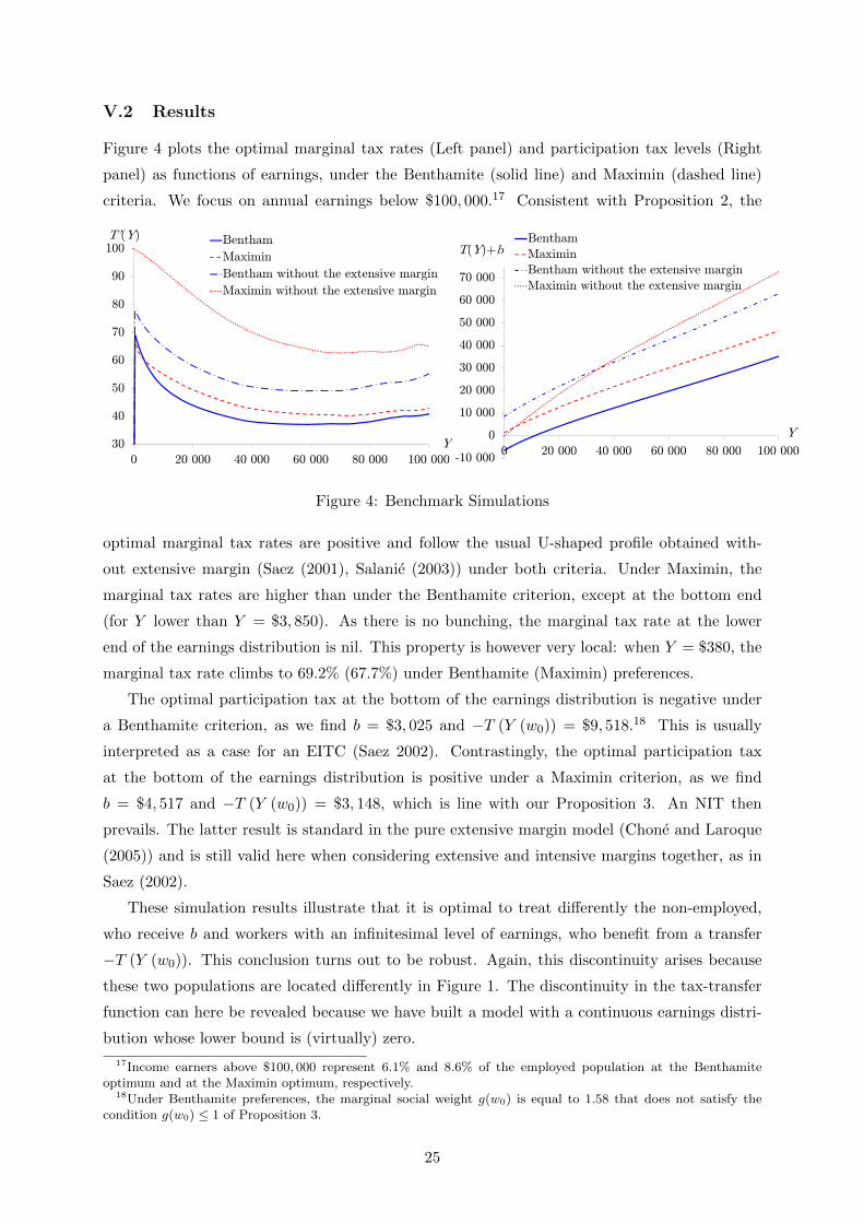
Figure 4 plots the optimal marginal tax rates (Left panel) and participation tax levels (Right

panel) as functions of earnings, under the Benthamite (solid line) and Maximin (dashed line)

criteria. We focus on annual earnings below $100, 000.17 Consistent with Proposition 2, the

100T’(Y) Bentham

Maximin

90

Maximin

Bentham without the extensive margin

M i i ith t th t i i80

Maximin without the extensive margin

70

60

50

40

300 20 000 40 000 60 000 80 000 100 000

Y

T(Y)+bBentham

Maximin

70 000

Maximin

Bentham without the extensive margin

Maximin without the extensive margin60 000

Maximin without the extensive margin

40 000

50 000

30 000

40 000

10 000

20 000

0

10 000

Y

-10 000

00 20 000 40 000 60 000 80 000 100 000

Figure 4: Benchmark Simulations

optimal marginal tax rates are positive and follow the usual U-shaped profile obtained with-

out extensive margin (Saez (2001), Salanie (2003)) under both criteria. Under Maximin, the

marginal tax rates are higher than under the Benthamite criterion, except at the bottom end

(for Y lower than Y = $3, 850). As there is no bunching, the marginal tax rate at the lower

end of the earnings distribution is nil. This property is however very local: when Y = $380, the

marginal tax rate climbs to 69.2% (67.7%) under Benthamite (Maximin) preferences.

The optimal participation tax at the bottom of the earnings distribution is negative under

a Benthamite criterion, as we find b = $3, 025 and −T (Y (w0)) = $9, 518.18 This is usually

interpreted as a case for an EITC (Saez 2002). Contrastingly, the optimal participation tax

at the bottom of the earnings distribution is positive under a Maximin criterion, as we find

b = $4, 517 and −T (Y (w0)) = $3, 148, which is line with our Proposition 3. An NIT then

prevails. The latter result is standard in the pure extensive margin model (Chone and Laroque

(2005)) and is still valid here when considering extensive and intensive margins together, as in

Saez (2002).

These simulation results illustrate that it is optimal to treat differently the non-employed,

who receive b and workers with an infinitesimal level of earnings, who benefit from a transfer

−T (Y (w0)). This conclusion turns out to be robust. Again, this discontinuity arises because

these two populations are located differently in Figure 1. The discontinuity in the tax-transfer

function can here be revealed because we have built a model with a continuous earnings distri-

bution whose lower bound is (virtually) zero.

17Income earners above $100, 000 represent 6.1% and 8.6% of the employed population at the Benthamiteoptimum and at the Maximin optimum, respectively.

18Under Benthamite preferences, the marginal social weight g(w0) is equal to 1.58 that does not satisfy thecondition g(w0) ≤ 1 of Proposition 3.

25

Finally optimal tax schedules without the extensive margin are also displayed under both

the Benthamite criterion (alternate line) and Maximin (dotted line). We exogenously fix the

distribution of skills and the number of non-employed at their calibrated levels given by Equation

(24). Canceling the extensive margin substantially increases the marginal tax rates. To quantify

this change, we compute the mean of marginal tax rates between 0 and $100, 000, weighted by

the density of workers. This mean increases by 13.0 percentage points under Bentham and by

8.9 percentage points under Maximin. As expected as well, the optimal marginal tax rate at

the lower bound is strictly positive (and very high) under Maximin when the extensive margin

is neglected.19 The right panel shows that under Benthamite preferences, the participation

tax becomes positive at the bottom of the earnings distribution when the extensive margin is

shut-down.

We also a conduct sensitivity analysis. First, a rise in the parameter σ increases the aversion

to inequality and this leads to a rise in marginal tax rates (see the left panel of Figure 5). The

right panel shows that the optimal participation tax at the low end of the earnings distribution

evolves ambiguously with σ. Intuitively participation taxes at the bottom are lower when the

welfare weight on the least skilled workers g (w0) becomes very important. However, with a

very high aversion to inequality, the welfare of the non-employed becomes dominant and g (w0)

decreases.

T’(Y) Bentham with s=0.5Bentham with s=0.8B h i h 1

65

70 Bentham with s=1Maximin

60

65

55

45

50

40

45

35

300 20 000 40 000 60 000 80 000 100 000

Y

T(Y)+b Bentham with s=0.5Bentham with s=0.8

40 000

Bentham with s 0.8Bentham with s=1Maximin

30 000

20 000

10 000

20 000

10 000

00 20 000 40 000 60 000 80 000 100 000

Y

-10 000

Figure 5: Simulations with different σ

Second, Figure 6 illustrates how the optimal tax schedule depends on the intensive labor

supply elasticity ε. When ε increases from 0.25 to 0.5, distortions along the intensive margin

become more important, so the solid curve in Figure 2 has to become flatter. The left panel

shows that marginal tax rates decrease when the elasticity of earnings ε increases from 0.25 to

0.5, under both Maximin and Benthamite preferences. The only exception is under Maximin for

earnings below $4, 700. The right panel emphasizes that participation taxes decrease (increase)

19In the absence of the extensive margin, the participation tax at the bottom end is adjusted so that the welfareof the non-employed is identical to the one of the least skilled worker. Consequently, there is a positive mass ofwelfare weights attached to these workers and the Boadway and Jacquet (2008)’s argument for positive marginaltax rate at the bottom applies.

26

with ε for earnings above (below) roughly around $30, 000, under both criteria.

85T’(Y)

Bentham

75

80 Maximin

Bentham with e=0.5

65

700 5

Maximin with e=0.5

55

60

65

45

50

55

35

40

45

30

35

250 20 000 40 000 60 000 80 000 100 000

Y

T(Y)+bBentham

M i i40 000

Maximin

Bentham with e=0.5

M i i ith 0 5

30 000

Maximin with e=0.5

20 00020 000

10 000

00 20 000 40 000 60 000 80 000 100 000

Y

-10 000

0 20 000 40 000 60 000 80 000 100 000

Figure 6: Simulations with different ε

Third, in addition to comparing what happens with and without the extensive margin (in

Figure 4), Figure 7 displays the result of a sensitivity analysis with respect to the profile of

the elasticity of participation. Instead of taking π0 = 0.5 and π1 = 0.4 in Equation (24), we

take π0 = 0.8 and π1 = 0.2, so as to concentrate participation responses more on low skilled

workers, while keeping the average elasticity of participation roughly unchanged. Consequently,

the dashed curve in Figure 2 becomes steeper under both social objectives. We thus expect that

marginal tax rates shift upwards and participation tax levels decrease at the bottom. Figure 7

confirms this intuition for earnings above $25, 000 under Benthamite and above $15, 000 under

Maximin.

70

T’(Y) Bentham

65

70Maximin

B th ith d i ti i ti

60

Bentham with a more decreasing participation elasticityMaximin with a more decreasing participation

55

Maximin with a more decreasing participation elasticity

50

45

40

350 20 000 40 000 60 000 80 000 100 000

Y

Bentham

M i iT(Y)+b Maximin

Bentham with a more decreasing

40 000

gparticipation elasticityMaximin with a more decreasing participation elasticity

30 000participation elasticity

20 000

10 000

0 Y

-10 000

0 20 000 40 000 60 000 80 000 100 000

Figure 7: Simulations with a more decreasing profile w 7→ π (w) in the current economy

The following properties appear robust across these sensitivity analyses: Marginal tax rates

are non negative and U-shaped; there is no bunching and our sufficient condition for positive

marginal tax rates (in the interior of the earnings distribution) holds under Maximin and Ben-

thamite criteria; participation taxes are positive under Maximin; participation taxes are negative

at the bottom of the earnings distribution under the Benthamite criterion.

27

VI Conclusion

This paper has derived a new method to sign distortions (along the intensive margin) in screening

models with random participation. It has focused on the design of the optimal income tax

schedule when labor supply responds along both the extensive and intensive margins. It has

also applied the new method to a range of other important adverse selection problems.

In the optimal taxation context, individuals are heterogeneous along two dimensions: Their

skill and their disutility of participation to the labor market. We have derived a mild sufficient

condition for non negative marginal tax rates over the entire skill distribution. We have also

derived conditions under with the participation tax should be positive everywhere.

Using U.S. data, we have implemented our optimal tax formula. The main conclusions of

our numerical analysis are twofold: Marginal tax rates should be non negative everywhere and

the participation tax should typically be discontinuous at zero earnings. So, when the optimal

participation tax is negative at the bottom of the earnings distribution, the optimal tax-transfer

schedule should jump at the lowest possible level of earnings, above which marginal tax rates

remain non negative. This suggests that the EITC phase-in range, where transfers increase

as earnings rise, would not be optimal. This numerical analysis has also emphasized that the

optimal tax schedule is U-shaped as in the literature without an extensive margin. However,

introducing a plausible extensive margin substantially reduces the marginal tax rates.

Appendices

A Proof of Lemma 2

As Y is assumed piecewise-differentiable, it is continuous. Hence, U is differentiable, so the co-

state variable q is differentiable as well. From Equation (11), a kink in function Y may induce a

kink in U ′. It may also correspond to a kink in the derivative of the co-state variable q′, however,

q′ remains continuous.

The proof of (18a), (18b) and (18c) follows Guesnerie and Laffont (1984) very closely. We

consider as the control variable the derivative denoted i (w) of gross earnings Y (.), we consider

as the state variables the gross utility levels U and gross earnings Y , with associated co-state

variables being denoted respectively as q and µ. Finally, we denote η (w) the Lagrange multiplier

associated to the monotonicity constraint i (w) = Y ′ (w) ≥ 0. From (14), the Hamiltonian of

this problem writes H (U (w) , Y (w) , q (w) , w, b, λ) + µ (w) · i (w) + η (w) · i (w). The optimality

conditions are:

i (w) : µ (w)a.e= −η (w) , η (w) i (w) = 0 , η (w) ≥ 0 , i (w) ≥ 0

Y (w) : −µ′ (w) = H′Y (U (w) , Y (w) , q (w) , w, b, λ) with µ (w0) = µ (w1) = 0

U (w) : −q′ (w) = H′U (U (w) , Y (w) , q (w) , w, b, λ) with q (w0) = q (w1) = 0

28

• If there is no bunching around skill w, constraint i (w) ≥ 0 is not binding, so µ (w) is

constant at zero in this neighborhood and µ′ (w) = 0 in this neighborhood. Consequently,

H′Y (U (w) , Y (w) , q (w) , w, b, λ) = 0 which gives (18a) using (16a).

• If there is bunching over a “maximal”interval [w,w], then there is no bunching at the

boundaries w and w. Consequently, µ (w) = µ (w) = 0 and∫ ww µ′ (w) · dw = 0. One thus

obtains∫ ww H

′Y (U (w) , Y (w) , q (w) , w, b, λ) · dw = 0, which leads to (18b) using (16a).

• For any w: −q′ (w) = H′U (U (w) , Y (w) , q (w) , w, b, λ) gives (18c) given (16b).

Finally, Equation (18d) is obtained using (16c) and the optimal condition on b, which is∫ w1

w0H′b (Y (w) , U (w) , q (w) , w, b, λ) dw = 1, as the left-hand side of (8) is not in the defini-

tion (14) of the Hamiltonian.

B Proof of Lemma 3

Let

τ (w) ≡ Y (w)− C (U (w) , Y (w) , w) + b− 1− g (w)

κ (w)

(1) From (20), the derivative of X (w) has the sign of τ (w) for all skill levels.

(2) From (11) and (12), function τ admits for all skill levels a left- and a right-derivative. It is

moreover differentiable at all skill levels where Y is differentiable with a derivative equal

to:

τ ′ (w) =

(1 +

U ′Y

U ′C

)· Y ′ (w)−

(1− g (w)

κ (w)

)′(25)

We now show that, under Property 1, X (w) ≤ 0 implies τ ′ (w) < 0. Assume X (w) ≤ 0.

Then, either there is bunching at w, in which case Y ′ (w) = 0, or Equation (18a) applies, in

which case 1 + U ′Y /U

′C is of the same sign as X (w), i.e. non positive. In both cases, from

Property 1 and Equation (25), we obtain τ ′ (w) < 0. At a kink in Y , τ is not differentiable.

However, the same expression as Equation (25) links the right- (left-) derivatives of τ , Y

and (1− g (w)) /κ (w). Applying the same reasoning, we obtain that the right- (left-)

derivatives of τ are negative if X (w) < 0.

Assuming X ′ (w) ≤ 0 and X (w) ≤ 0 implies that at w, τ is non-positive (from (1)) and

admits a negative right-derivative (from (2)). There thus exists an open interval whose lower

bound is w where τ , thereby X ′ are negative. X is thus negative and strictly decreasing on this

interval. Let (w, w∗) be a maximal interval on which X ′ (w) < 0 with w < w∗ ≤ w1. We thus

have that X (w∗) < X (w) ≤ 0, which implies τ ′ (w) < 0 on [w, w∗]. Consequently, τ (w∗) < 0,

so one must have X ′ (w∗) < 0. Therefore X (w) cannot stop decreasing on [w, w1], which ends

the proof of Point a) of the Lemma. The proof of Point b) is symmetric.

29

References

[1] Atkinson, T., 1990, Public Economics and the Economic Public, European Economic Re-view, 34(2-3), 225-48.

[2] Baron, D. P. and R. B. Myerson, 1982, Regulating a Monopolist with unknowns costs,Econometrica, 50(4), 911-30.

[3] Boadway, R. and L. Jacquet, 2008, Optimal Marginal and Average Income Taxation underMaximin, Journal of Economic Theory, 143(1), 425-41.

[4] Boadway, R., M. Marchand, P. Pestieau, M. Del Mar Racionero, 2002, Optimal Redistri-bution with heterogenous preferences for leisure, Journal of Public Economic Theory, 4(4),475-98.

[5] Boone, J. and L. Bovenberg, 2004, The optimal taxation of unskilled labour with job searchand social assistance, Journal of Public Economics, 88(11), 2227-58.

[6] Chone, P. and G. Laroque, 2005, Optimal incentives for labor force participation, Journalof Public Economics, 89(2-3), 395-425.

[7] Chone, P. and G. Laroque, 2010, Negative marginal tax rates and heterogeneity, AmericanEconomic Review, 100(5), 2532-47.

[8] Chone, P. and G. Laroque, 2011, Optimal Taxation in the extensive model, Journal ofEconomic Theory, 146(2), 425-53.

[9] Cuff, K., 2000, Optimality of Workfare with Heterogeneous Preferences, The CanadianJournal of Economics, 33(1): 149-174.

[10] Diamond, P., 1980, Income Taxation with Fixed Hours of Work, Journal of Public Eco-nomics, 13(1), 101-10.

[11] Diamond, P, 1998, Optimal Income Taxation: An Example with a U-Shaped Pattern ofOptimal Marginal Tax Rates, American Economic Review, 88(1), 83-95.

[12] Guesnerie, R., 1995, A Contribution to the Pure Theory of Taxation, Cambridge UniversityPress, Cambridge.

[13] Guesnerie, R. and J-J. Laffont, 1984, A complete solution to a class of principal-agent prob-lems with an application to the control of a self-managed firm, Journal of Public Economics,25(3), 329-69.

[14] Hammond, P., 1979, Straightforward Individual Incentive Compatibility in LargeEconomies, Review of Economic Studies, 46(2), 263-82.

[15] Heckman, J., 1993, What Has Been Learned about Labor Supply in the Past Twenty Years?,American Economic Review, 83(2), 116-21.

[16] Hellwig, M., 2007, A contribution to the theory of optimal utilitarian income taxation,Journal of Public Economics, 91(7-8), 1449-77.

[17] Hellwig, M., 2010, Incentive Problem with Unidimensional Hidden Characteristics: a Uni-fied Approach, Econometrica, 78(4), 1201-37.

[18] Immervoll, H., Kleven, H., C.T. Kreiner and E. Saez, 2007, Welfare reforms in Europeancountries: a Microsimulation analysis, Economic Journal, 117(516), 1-44.

30

[19] Juhn, C., K.M. Murphy, R.H. Topel, J.L. Yellen and M.N. Baily, 1991, Why has the NaturalRate of Unemployment Increased over Time?, Brookings Papers on Economic Activity,1991(2), 75-142.

[20] Kleven, H.J. and C. T. Kreiner, 2006, The Marginal Cost of Public Funds: Hours of Workversus Labor Force Participation, Journal of Public Economics, 90(10-11), 1955-73.

[21] Kleven, H.J., C. T. Kreiner and E. Saez, 2009, The Optimal Income Taxation of Couples,Econometrica, 77(2), 537-60.

[22] Lorenz, N and D. Sachs, 2011, Optimal Nonlinear Redistributive Taxation with MinimumHours of Work, mimeo, University of Konstanz.

[23] Maskin, E. and J. Riley, 1984, Monopoly with incomplete information, Rand Journal ofEconomics, 15(2), 171-96.

[24] Meghir C. and D. Phillips, 2008, Labour Supply and Taxes, IZA discussion paper 3405.

[25] Mirrlees, J., 1971, An Exploration in the Theory of Optimum Income Taxation, Review ofEconomic Studies, 38(2), 175-208.

[26] Mussa, M. and S. Rosen, 1978, Monopoly and Product Quality, Journal of Economic The-ory, 18, 301-17.

[27] Polachek, S.W. and W.S. Siebert, 1993, The Economics of Earnings, Cambridge UniversityPress.

[28] Rochet, J-C., 2009, Monopoly regulation without the Spence-Mirrlees assumption, Journalof Mathematical Economics, 45(9-10), 693-700.

[29] Rochet, J-C. and L. Stole, 2002, Nonlinear Pricing with Random Participation, Review ofEconomic Studies, 69(1), 277-311.

[30] Sadka, E., 1976, On income distribution, incentive effects and optimal income taxation,Review of Economic Studies, 43(2), 261-67.

[31] Saez, E., 2001, Using Elasticities to Derive Optimal Income Tax Rates, Review of EconomicsStudies, 68(1), 205-29.

[32] Saez, E., 2002, Optimal Income Transfer Programs: Intensive Versus Extensive LaborSupply Responses, Quarterly Journal of Economics, 117(3), 1039-73.

[33] Saez, E., Slemrod, J. and S. Giertz, 2010, The Elasticity of Taxable Income with Respectto Marginal Tax Rates: A Critical Review, Journal of Economic Literature, forthcoming.

[34] Salanie, B., 2003, The Economics of Taxation, MIT Press.

[35] Seade, J., 1977, On the shape of optimal tax schedules, Journal of Public Economics, 7(2),203-35.

[36] Seade, J., 1982, On the sign of the optimum marginal income tax, Review of EconomicStudies, 49(2), 637-43.

31