A sparse Bayesian approach for joint feature selection and classifier learning

Pattern Analysis and Applications manuscript No.(will be inserted by the editor)

A Sparse Bayesian Approach for Joint Feature

Selection and Classifier Learning

Agata Lapedriza1,2, Santi Seguı1, David Masip1,3, Jordi Vitria1,4

1 Computer Vision Center, Universitat Autonoma de Barcelona

Edifici O Bellaterra 08193, Spain

agata,ssegui,[email protected]

2 Dept. Informatica,Universitat Autonoma de Barcelona

Edifici O Bellaterra 08193, Spain

3 Universitat Oberta de Catalunya

Estudis d’Informatica Multimedia i Telecomunicacio

Rambla del Poblenou 156, 08018 Barcelona, Spain.

[email protected]

4 Dept. Matematica Aplicada i Analisi, Universitat de Barcelona

Gran Via de les Corts Catalanes 585, Barcelona (Spain)

Received: date / Revised version: date

Abstract In this paper we present a new method for Joint Feature Se-

lection and Classifier Learning (JFSCL) using a sparse Bayesian approach.

These tasks are performed by optimizing a global loss function that includes

a term associated with the empirical loss and another one representing a fea-

2 Agata Lapedriza1,2, Santi Seguı1, David Masip1,3, Jordi Vitria1,4

ture selection and regularization constraint on the parameters. To minimize

this function we use a recently proposed technique, the Boosted Lasso algo-

rithm, that follows the regularization path of the empirical risk associated

with our loss function. We develop the algorithm for a well known non-

parametrical classification method, the Relevance Vector Machine (RVM),

and perform experiments using a synthetic data set and three databases

from the UCI Machine Learning Repository. The results show that our

method is able to select the relevant features, increasing in some cases the

classification accuracy when feature selection is performed.

1 Introduction

Binary classification problems take as input a training data set D = (xn, yn)n=1,..N ,

where xi ∈ Rd is a sample (being d the subspace dimensionality) and yi is

an integer value representing its corresponding label. The goal is to learn

a classifier that predicts the correct label of any unseen sample x ∈ Rd.

Usually the data dimensionality d is large, which increases the difficulty

of the classifier parameters estimation. This phenomenon is known as the

curse of dimensionality [1,2], and it has been shown that the number of

samples needed to learn a reliable classifier increases exponentially with the

dimensionality d. To overcome this drawback, two different approaches are

followed in the current machine learning research: (i) to use robust classifi-

cation rules, such as Support Vector Machines [3], boosting variants [4] or

Bayesian logistic regression approaches [5], and (ii) to perform a previous

Feature selection 3

preprocessing step on the input data, obtaining the most informative feature

subset for the classification task [6,7]. When only a subset of features from

the original data are preserved, the process is known as feature selection [8],

while when the original features are combined by applying a learned map-

ping to a reduced space the process is known as feature extraction [9–11].

Feature selection has been shown to improve generalization when many

irrelevant features are present. According to Guyon and Elisseeff work [12],

feature selection approaches are divided into filters, wrappers and embedded

approaches. Most common approaches are filters, which act as a preprocess-

ing step independently of the final classifier. In contrast, wrappers take the

classifier into account as a black box. Finally, embedded approaches simul-

taneously determine features and classifier during the training process.

There are specifically tailored methods for feature selection in non-

parametric classifier learning. Guyon et al. [13] proposed a feature ranking

method for Support Vector Machines where the selection is performed by

Recursive Feature Elimination (RFE). Mao [14] used a pruning strategy for

the same Support Vector Machines framework. In the same context Chen et

al.[15] used the Fisher ratio in a forward feature selection for constructing

sparse kernels.

Hong and Mitchell [16] used the leave-on-out criteria in a backward

selection algorithm applied to post-processing procedures for classification

problems while Weston et al. [17] used the gradient descent method over

an upper bound of the leave-one-out error for selecting the optimal sub-


space. On the other hand, Automatic Relevance Determination (ARD) [18]

has been used to estimate scaling factors on features in different types of

classifiers. In kernel classifiers such as Support Vector Machines a Bayesian

method for model selection was proposed by Seeger [19], where a maximum

a posteriori (MAP) criterion on the parameters is imposed using a vari-

ational approach. Nevertheless, there exist only a few embedded methods

addressing the feature selection problem in connection with non-parametric

classifiers up to now. An embedded approach for the quadratic 1-norm SVM

was suggested by Zhu et al. [20], while Jebara and Jaakkola [21] developed

a feature selection method as an extension to the so-called maximum en-

tropy discrimination. Li at al [22] used a two stepwise forward procedure

for the same compacting model problem. Recently, Krishnapuram et al. [23]

developed a joint classifier and feature optimization method for kernel clas-

sifiers. The method shows promising results in high dimensional data sets.

Nevertheless, the resulting kernel classifier model is learned by the Expec-

tation Maximization algorithm and the computational complexity becomes

unpractical for large training data sets.

In this paper we propose an embedded method to jointly perform feature

selection and classification for a well known non-parametric classifier, the

Relevance Vector Machine (RVM) [24]. Our method uses a Laplace prior,

through an L1 penalty or constraint, to promote sparsity on the RVM pa-

rameters as well as in the distribution of selected features. Tibshirani et al.

[25] were the first to propose this prior to achieve sparse parameter esti-

Feature selection 5

mates in the regression context. Since then, the use of constraints based on

the absolute values of coefficients has been used to achieve sparseness in a

variety of learning tasks, such as L1-SVM or Logistic Regression Learning

[5]. However, Laplace priors produce a loss function that is not differen-

tiable, so that we can not use any gradient or higher order derivatives to

minimize our loss function.

Recently, a new method for coordinate descent that does not rely on

derivatives has been proposed for the optimization of general convex loss

functions penalized through an L1 constraint [26]. This algorithm, known

as Boosted Lasso (BLasso) [27], can be easily extended to the case of a

general loss penalized by a general convex function. Our main contribution

in this work is the use of a BLasso approach to jointly perform the feature

selection and the classifier training tasks.

This paper is organized as follows. In the next section we give a brief

review of the main statistical tools used in this work: the Vector Machines

classifiers, the Lasso problem and the BLasso algorithm, which yields to the

proposed new approach of the RVM, the Laplacean-RVM (L-RVM). Section

3 describes the proposed Joint Feature Selection and Classifier Learning

method (JFSCL). In section 4 we expose some experimental results for

different purposes: (i) comparison of classical RVM approach with L-RVM,

(ii) comparison of L-RVM with the proposed JFSCL, and (iii) comparison

of JFSCL with some of the state-of-the-art feature selection filters. Moreover

we also analyze the sensitivity of the proposed JFSCL with respect to the


design parameters of the method. Finally section 5 concludes this work

showing also some future lines of research.

2 Sparse Bayesian Learning using Laplace Priors

In this paper we present an embedded method to jointly perform the feature

selection and classifier training tasks in a Bayesian framework. Although

we will work on a specific classifier for this purpose (RVM), the proposed

framework could be used for almost any non-parametric classifier. The elec-

tion of the RVM classifier is justified by its performance in general learning

problems as well as by its elegant adaptation to the sparse Bayesian learn-

ing framework. This classifier fares similar to the “best of-the-shelf” SVM

classifier when considering its classification performance while overcomes

SVM main drawbacks: it gets a real sparse vector selection, it has a lower

computational cost and it is less prone to overfitting [24].

2.1 Vector Machines

Support Vector Machine (SVM) [28] is one of the most successful classifiers

developed in the pattern recognition field. Briefly, considering a 2-classes

classification problem, a SVM predicts the expected labels as

y(x) = χ(0,∞)(N∑

n=1

wnK(x, xn) + w0) (1)

being χ(0,∞) : R → R the characteristic function (defined to be identi-

cally 1 on (0,∞) and 0 elsewhere), K a kernel function, and w = (w0, ..., wN )

Feature selection 7

the weights vector that should be learned to minimize the empirical classifi-

cation error. The maximization of the margin criterion has been shown to be

an appropriate property to reduce the generalization error, and some upper

bounds have been defined in the literature [28]. Nevertheless, the method

suffers from some limitations, such as:

– predictions are binary, and no probabilistic value can be derived from

the classification of a sample.

– usually, the number of selected support vectors is small, but no specific

prior is imposed on the solution to control the desired sparsity level.

– in general, the solution that minimizes the training error is not the

solution with maximum margin, and thus this solution is not the one

with expected minimum generalization error. A trade off parameter is

needed to fix this optimal operation point. This process can only be

solved by cross validating the training set, being the tuning process

computationally costly.

– there is a variety of kernel functions K to use, but they must satisfy the

Mercer’s condition.

To overcome these drawbacks, Tipping [24] proposed the RVM classi-

fier, where a Bayesian approach for learning the parameters w is followed.

Briefly, he suggested the use of a set of hyperparameters associated to the

generation of the weights w, obtaining a sparse distribution on w. The ex-

perimental results show a generalization capability close to the SVM, using

an impressively few number of support vectors.


As a first step to our objective, we propose the use of a Laplace prior

to promote sparsity on the Relevant Vector Machine parameters. Formally,

and given the samples of a 2-classes classification problem, let us adopt a

Bernoulli probabilistic distribution on the prediction of the RVM as follows

P (y = 1|x) = σ(N∑

n=1

wnK(x, xn) + w0) (2)

where σ : R→ R is the sigmoid function, σ(a) = 1/(1+exp (−a)), for all

a ∈ R. From the definition of a Bernoulli distribution we have P (y = 0|x) =

1−P (y = 1|x), and the negated log-likelihood estimator for the parameters

set w = (w0, ..., wN ) is

L(D,w) = −N∑

i=1

σ(N∑

n=1

wnK(xi, xn)+w0)yn(1−σ(N∑

n=1

wnK(xi, xn)+w0)1−yn)

(3)

To promote sparsity on the selected vectors we can penalize the loss

function L(D,w) through a constraint such as R(w) = ‖w‖1, getting the

following loss function

G(w) = L(D,w) + λR(w) (4)

being λ a positive real value. In this formulation the estimate for w

when using this model can be interpreted as a Bayesian posterior mode esti-

mate when the prior on the parameters are independent double-exponential

(Laplace) distributions [26].

Feature selection 9

There are two aspects of this new RVM approach to be studied in order

to become a real alternative to the original one: (i) how to compute a feasible

solution, and (ii) how this solution compares to the solution obtained by

classical RVM.

Notice that this RVM approach corresponds to a Lasso problem, that is,

a Loss Function with a penalty on the L1-norm of the parameters. In the

next subsection we describe in detail the Lasso problem and include a brief

survey on Lasso methods and their applications.

2.2 The LASSO Problem

Traditional approaches to learning methods seek to optimize a function as-

sociated to the empirical error rate. For example, most of the statistical

procedures use likelihood or negated likelihood estimators to learn the pa-

rameters of the model. However, given that the training data is usually a

finite set, learning algorithms could lead to an arbitrary complex model

as a consequence of the training error minimization, obtaining in that way

a classifier that presents high variance on unseen data and poor classifi-

cation results on the testing data. To avoid this fact some regularization

constraints on the parameter set can be jointly imposed during the training

step. Thus, the learning method optimizes a loss function subject to some

model complexity restriction.

Lasso is a regularization approach for parameter estimation originally

proposed by Tibshirani [26] that shrinks a learned model through an L1


penalty on the parameters set. Formally, in a statistical classification frame-

work with parameters w, the Lasso loss can be expressed as

G(w, λ) = L(D,w) + λR(w) (5)

where L(D,w) is the negated empirical error rate, R(w) is the imposed

L1 restriction on the parameters, R(w) = ‖w‖1 ∈ R, and λ is a positive real

value. In fact, the sum term λR(w) is the negated log-likelihood obtained

when we impose a centered Laplace distribution (with variance inversely

proportionally to λ) on the components of w. Consequently, this constraint

imposes sparsity on the w components, and the parameter λ is controlling

the regularization level on the estimate. Observe that parameter λ is a

crucial selection to get a good solution. Notice that setting λ = 0 reverses

the Lasso problem to minimizing the unregularized loss while a very large

value will completely shrink the parameters to 0, leading to an empty model.

Based on the seminal paper of Tibshirani [26], different computational

algorithms have been developed to solve the regularization path. Osborne

et al. [29,30] developed the homotopy method for the squared loss function

case and Efron et al. the LARS method [31].

Lasso has been successfully applied to multiple disciplines. In the bioin-

formatics field Vert et al. [32] adapted the Lasso sparse modeling to the

problem of siRNA efficacy prediction. Tibshirani et al. [33] applied their

fussed Lasso algorithm to protein mass spectroscopy and gene expression

Feature selection 11

data, while Ghosh and Chinnaiyan [34] adapted the Lasso algorithm to the

selection and classification of genomic biomarkers.

Finally, Zhao and Yu combine boosting and Lasso approximating the

Lasso path in general situations. Their Boosted Lasso approach [27] has

the computational advantages of Boosting converging to the Lasso solution

with global L1 regularization. This methodology has been recently applied

to text classification [35] (reporting a significant improvement with respect

to classic parameter estimation), handwritten character recognition [36],

and intestinal motility analysis [37].

2.3 The Boosted Lasso Algorithm (BLasso)

The Boosted Lasso (BLasso) algorithm is a numerical method developed by

Zhao and Yu [27] that finds a solution for general Lasso problems. Moreover,

the algorithm can automatically tune the parameter λ. This method consists

of a forward step similar to the statistical interpretation of a well-known

learning method, Boosting [38], where an additive logistic regression model

is sought using a maximum likelihood approach as a criterion. Moreover,

there is a backward step that makes the algorithm able to correct mistakes

made in early stages. This step uses the same minimization rule as the

forward step to define each fitting stage with an additional restriction that

forces the model complexity to decrease. The algorithm is specified in table

1. The constant ε, which represents the step size, controls the fineness of

the grid BLasso runs on. On the other hand, the tolerance ξ controls how


big a descend needs to be made for a backward step to be taken. This

parameter should be much smaller than ε to have a good approximation

and can be even set to 0 when the base learners set is finite. In that case,

there is a theorem stated and proved in [27] that guarantees the convergence

of the algorithm to the Lasso path when ε tends to 0 and the empirical loss

L(D,w) is strictly convex and continuously differentiable in w.

BLasso can be easily extended to deal with convex penalties other than

the L1 restriction. This extended version, that is known as the Generalized

Boosted Lasso algorithm, was also proposed by Zhao and Yu [27] and the

procedure of the system remains the same. However, for general convex

penalties, a step on different coordinates does not necessarily have the same

impact on the penalty. For this reason one is forced to work directly with the

penalized function, what generates small changes in the resulting algorithm

as can be seen in [27].

2.4 The Laplacean Relevance Vector Machine (L-RVM)

As stated in section 2.1, a new formulation of the RVM is done by the

optimization of the global loss function

G(w) = L(D,w) + λR(w) (6)

being L(D,w) the negated log-likelihood estimator for the parameters

set w (see equation 3), and R(w) = ‖w‖1 a constraint to promote sparsity

on w. Given that this optimization corresponds to a Lasso problem, we


Table 1 Boosted Lasso Algorithm(BLasso)

Notation

va, a ∈ A = 1, ..., d is a vector with having all 0s except a 1 in the position a.

Inputs:

– ε > 0: small step size

– ξ ≥ 0: small tolerance parameter.

Initialization

– (a, s) arg mina∈A,s=±ε

Pni=1 L(Zi; sva)

– w0 = sva

– λ0 = 1ε(Pn

i=1 L(Zi; 0)−Pni=1 L(Zi; w

0))

– I0 = a

– r = 0

Iterative Step

– Compute (a) arg mina∈(Ir)

Pni=1 L(Zi; w

r + sava) where sa = −sign(wra)

– If G(Br + sa1j , λr)−G(wr, λr) < −ξ then

– wr+1 = wr + sa1j and λr+1 = λr.

– Otherwise

– (a, s) = arg mina∈A,s=±ε

Pni=1 L(Zi; wr + sva)

– wr+1 = wr + sva

– λr+1 = minλr, 1ε(Pn

i=1 L(Zi; wr)−Pn

i=1 L(Zi; wr+1))

– Ir+1 = Ir ∪ a

End: Stop when λr ≤ 0.


propose to minimize this function using the BLasso described in section 2.3.

This new formulation of the RVM will be called the Laplacean Relevance

Vector Machine and denoted by L-RVM.

3 Joint Feature Selection and Classifier Learning Method

(JFSCL)

The classification accuracy of a classifier can be improved by performing

an appropriate feature selection and determining which is the most suitable

subset of variables to be considered during the classification process. For

this purpose we extend the method proposed in section 2.4 by adding a new

parameters vector that will control the activation of the relevant features.

More concretely, we add a new sum term in the regularization part of the

global loss function (6) obtaining a new cost function that can also be

optimized using the described BLasso algorithm.

To control the activation of the features we consider a function σdk :

Rd → Rd defined as follows

σdk(a)(σk(a1), ..., σk(ad)),∀a(a1, ..., ad) ∈ Rd (7)

where k is any positive real value and σk : R→ R is the sigmoid function,

σk(a) =1

1 + exp (−ka),∀a ∈ R (8)

Let be v = (v1, ..., vd) a new parameters vector and x ∈ Rd an input

data. Then consider the following expression


σdk(v)¯ x : (σk(v1)x1, ..., σk(vd)xd) (9)

where ¯ denotes the Hadamard product. Observe, from the definition

of the sigmoid function (equation 7), that the components of σdk(v) take, in

general, values very close to 0 or very close to 1, supposing that k is high

enough. Thus, equation (9) can express an activation or a deactivation of

the ith feature by its corresponding parameter vi.

After these definitions and observations we can consider a new global

loss function for the RVM that is constrained by an extended parameter set

Ω = (w,v):

Γ (Ω) = L(D,w,v) + λ1‖w‖1 + λ2‖σdk(v)‖1 (10)

This loss function represents a preference for solutions that use a small

set of components from a small set of samples. In this case, a reasonable

choice is to impose the same value for both regularization terms, λ := λ1 =

λ2. Therefore we obtain the following expression of the loss:

Γ (Ω) = L(D,w,v) + λ(‖w‖1 + ‖σdk(v)‖1) (11)

that can be minimized using the extended version of BLasso, the above

mentioned Generalized Boosted Lasso. This approach will be called the

Joint Feature Selection and Classifier Learning method (JFSCL).


4 Experiments

In this section we evaluate different aspects of the proposed methodologies.

For this aim we use synthetic data and three public databases from the UCI

Machine Learning Repository [39] that are binary: the PIMA Dabetes, the

Breast Cancer and the Heart disease.

First of all we evaluate the performance of the proposed L-RVM and

we compare it with the classical RVM approach. After that, we test the

proposed JFSCL using synthetic data and perform some experiments to

evaluate the sensitivity of the method to the design parameters. Finally

we test the performance of the JFSCL with real data and compare this

proposed method with other feature selection filters.

4.1 Classical RVM and L-RVM

In this section we will test the performance of the L-RVM that has been

proposed in section 2.4. We have used a Gaussian kernel function K(x1, x2):

K(x1, x2) = exp(−γ‖x1 − x2‖2) (12)

being γ an appropriate positive real value that has been determined by

cross validation.

We have performed experiments with three public databases from the

UCI Machine Learning Repository, the PIMA Diabetes, the Breast Cancer,

and the Heart disease data. To train and test the methods we have used pub-

lic data sets from http://ida.first.fraunhofer.de/projects/bench/benchmarks.htm


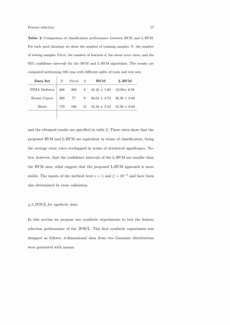
Table 2 Comparison of classification performance between RVM and L-RVM.

For each used database we show the number of training samples N , the number

of testing samples Ntest, the number of features d, the mean error rates, and the

95% confidence intervals for the RVM and L-RVM algorithms. The results are

computed performing 100 runs with different splits of train and test sets.

Data Set N Ntest d RVM L-RVM

PIMA Diabetes 468 300 8 24.10 ± 1.06 23.98± 0.58

Breast Cancer 200 77 9 26.04 ± 4.74 26.30 ± 0.80

Heart 170 100 13 16.34 ± 3.53 16.30 ± 0.68

and the obtained results are specified in table 2. These rates show that the

proposed RVM and L-RVM are equivalent in terms of classification, being

the average error rates overlapped in terms of statistical significance. No-

tice, however, that the confidence intervals of the L-RVM are smaller than

the RVM ones, what suggest that the proposed L-RVM approach is more

stable. The inputs of the method were ε = 1 and ξ = 10−5 and have been

also determined by cross validation.

4.2 JFSCL for synthetic data

In this section we propose two synthetic experiments to test the feature

selection performance of the JFSCL. This first synthetic experiment was

designed as follows: d-dimensional data from two Gaussian distributions

were generated with means:


−4 −3 −2 −1 0 1 2 3 4−4

−3

−2

−1

0

1

2

3

4

−4 −3 −2 −1 0 1 2 3 4−4

−3

−2

−1

0

1

2

3

4

(a) Scatter of the two first features from the Gaussian set (b) Scatter of two noise features from the Gaussian set

Fig. 1 Scatter of samples from the synthetic Gaussian data set. Symbol (+)

represents points from class 1 and symbol (.) represents points from class 2.

µ1 = [1√2,

1√2, 0, . . . , 0] (13)

µ2 = [− 1√2,− 1√

2, 0, . . . , 0] (14)

and standard deviation 1 for all the components (notice that the distance

between the d-dimensional Gaussian distribution centroids is 2). According

to the optimal linear classifier, the theoretical Bayes error can be computed

exactly for these two sets, and its value is 15.19. In the experiment, 200

samples (100 from each class) have been used for training the classical RVM,

the proposed L-RVM, and the proposed JFSCL. The test set was composed

by 1000 samples (500 from each class). An example of the scatter of the

first two features and two noise features is shown in Figure 1.


5 10 15 20 25 30 35 400.16

0.17

0.18

0.19

0.2

0.21

0.22

dimensions

erro

r ra

te

RVM

L−RVM

JFSCL

Fig. 2 Comparison of classification performance between RMV, L-RVM and JF-

SCL using the synthetic Gaussian data set. The X axis represents the data di-

mension, note that the only important dimensions are the two first ones, and the

rest dimensions are Gaussian noise. The Y axis represent the obtained mean error

rate over 20 runs.

Figure 2, shows the mean error rate of 20 random generations of the same

experiment, as a function of the space dimensionality. As can be observed,

the influence of adding spurious features on the RVM and L-RVM confuses

the classifier, while our approach keeps a quite constant error rate that is

close to the Bayes error. Moreover, our method focuses the classifier on the

first two features (the ones with class separability information).

In addition, a second set of synthetic databases has been generated in

order to test our proposal when data clusters are highly overlapped. Two

d-dimensional Gaussian data clusters (one per class) were generated for

d = 2, 10, 20, 30, 40 with means


Table 3 Mean error rate using the synthetic Gaussian data sets, varying the

distance between the Gaussian centroids to get different overlapping levels between

the classes. The error rate is shown as a function of both data dimensionality and

inter-class centroid distance.

Centroid distance

0.25

0.5

0.75

1

L-RVM

Dimensionality

2 10 20 30 40

41.09 43.09 44.92 45.52 46.25

32.24 33.87 35.46 36.35 38.26

23.42 24.27 26.13 27.06 28.74

15.94 17.49 19.21 20.07 21.20

JFSCL

Dimensionality

2 10 20 30 40

42.68 42.61 43.82 44.33 44.92

32.05 33.42 33.48 34.24 34.29

23.19 23.44 23.87 23.93 24.47

15.78 16.16 16.71 16.73 17.22

µ1 = [µ11, µ12, 0, . . . , 0] (15)

µ2 = [µ21, µ22, 0, . . . , 0] (16)

and standard deviation 1 for all the components. We vary the distance

between the centroids (µ11, µ12) and (µ21, µ22) from 0.25 to 1, having thus

different class overlapping levels. The experiments have been performed with

the L-RVM classifier and our proposed JFSCL method, and results can be

seen in table 3. Notice that our proposal fares significantly better in almost

all the cases, specially when the data dimensionality is high.


4.3 Analyzing the JFSCL Sensitivity to the Parameters Selection

In the proposed JFSCL there are two parameters that have to be fixed: (i)

k, that controls the steepness of the sigmoid function, and (ii) ε, the step

of the BLasso algorithm. Another parameter of the BLasso is the tolerance

ξ, but in all the cases it has been fixed at 10−5 and small variations of this

parameter do not affect the JSFCL.

In order to analyse the sensitiveness of the classification performance to

variations of these design parameters, we have performed the same experi-

ment for different values of k and ε. In particular we have performed these

experiments with the 40-dimensional train and test sets used in section 4.2,

having in this case 38 spurious components. These data were composed by

20 pairs of train and test sets, having 200 samples (100 per class) and 1000

samples (500 per class) respectively.

The means of the obtained error rates are shown in table 4. Notice that

there is no much variation in the results, although in this case ε = 1.2 and

k = 10 is the best option. Moreover, in all the cases except for k = 1, ε =

0.4 the obtained results are better than in the case of RV M (see this

results in figure 2). In these experiments the worst parameters combination

in terms of accuracy is k = 1, ε = 0.4. We think that here the main

problem is that the method can not significantly activate and/or deactivate

a feature in one step. That suggest that there have to be a compromise

between these two parameters. On the other hand, for ε greater than 50 the

method do not converge for any of the considered k values.


Table 4 Mean error rates obtained in the classification of the 40-dimensional

synthetic data with different values for the design parameters of the method.

Parameter ε corresponds to the step parameter in the BLasso algorithm, and the

k is the parameter of Eq.7

k = 1 k = 10 k = 20 k = 40 k = 80 k = 100 k = 500

ε = 0.4 26.39 17.59 17.66 17.20 16.58 17.44 17.61

ε = 0.8 17.20 17.36 17.98 16.31 16.53 16.89 17.13

ε = 1.2 16.77 16.01 16.41 16.48 16.40 17.02 18.56

ε = 2 17.25 16.92 17.15 17.18 16.99 17.35 16.98

ε = 5 17.42 17.52 16.40 16.62 16.70 16.39 17.38

ε = 10 17.97 16.91 17.08 17.09 17.71 19.39 17.91

4.4 UCI Machine Learning Repository using the proposed JFSCL

In this section we test the proposed JFSCL method using the PIMA Dia-

betes, the Breast Cancer and the Heart disease databases. The train and

test data sets are exactly the same as in section 4.1 to be able to compare

the error rate obtained when classical RVM or L-RVM are used. The results

are shown in table 5, where the mean in percentage of rejected features is

also specified. We can see that the error rates are equivalent to the cases

considered in section 4.1, comparing both tables 5 and 2. Nevertheless, the

JFSCL method allows us to reduce the number of used features to the half

of the original set.


Table 5 Obtained results (mean error rate and 95% confidence interval) using

the JFSCL, and mean number of rejected features (in percentage).

DataSet JFSCL Error rate Rejected Features

PIMA Diabetes 24.23 ± 0.34 48.33%

Breast Cancer 26.52 ± 0.92 41.25%

Heart 16.28 ± 0.65 31.15%

4.5 Comparison with Feature Selection Filters

In order to test the influence of the embedded feature selection in our JFSCL

method, we performed the same experiments using other state-of-the-art

feature selection techniques. In all the cases we ran the feature selection

algorithm selecting from one up to the maximum number of features (all

the possibilities) and then performed the classification with the L-RVM

classifier.

We have applied the following feature selection filters: (i) Forward Fea-

ture Selection (FFS) [40],(ii) Backward Feature Selection (BFS) [6], (iii)

Feature Ranking (FR) using 1-Nearest Neighbour leave-one-out [12], and

Floating Search (FS) [41].

The results obtained in these tests are shown in tables 6, 7, 8. Notice that

in the experiments performed with the Heart database, the JFSCL performs

always better than the other methods. However, with the other databases

there are methods that perform as well as the proposed JFSCL. For in-

stance, with the PIMA Diabetes database the best accuracy is obtained

with Feature Ranking using 5 features, being the error 23.74%. Neverthe-


Table 6 Obtained results (mean error and 95% confidence interval) using the

state-of-the-art feature selection methods with PIMA Diabetes Database. Notice

that the proposed JFSCL method selected in this case 51.66% of the features

(between 4 and 5 components) and obtained an error of 24.23± 0.34.

1 2 3 4 5 6 7

FSF 33.11 25.19 24.46 24.48 24.51 24.15 24.40

± 0.57 ± 0.49 ± 0.43 ± 0.37 ± 0.38 ± 0.35 ± 0.39

BSF 30.66 25.38 24.98 24.66 24.56 24.31 24.26

± 0.78 ± 0.45 ± 0.51 ± 0.37 ± 0.43 ± 0.36 ± 0.36

FR 33.11 28.59 23.90 23.37 23.74 23.95 24.20

± 0.57 ± 0.71 ± 0.52 ± 0.32 ± 0.32 ± 0.33 ± 0.32

FS 26.46 26.43 25.86 24.91 24.60 24.78 24.66

± 0.24 ± 0.27 ± 0.28 ± 0.23 ± 0.24 ± 0.22 ± 0.21

less, although this result is slightly better that the 24.23% obtained with

the JFSCL, the difference is not statistically significant, given that the con-

fidence intervals are overlapped. On the other hand, notice that the tested

state-of-the-art feature selection methods are not able to automatically fix

the number of needed features, while the proposed JFSCL can automati-

cally select both the features and the number of features. Moreover, these

results suggest that the number of features selected by the JFSCL is the

most appropriated. For instance, in the case of PIMA Diabetes Database

the best accuracy is obtained using 5 features and the JFSCL selects in this

case between 4 and 5 features. A similar behavior can be observed in the

results obtained with the other databases.



state-of-the-art feature selection methods with Breast Cancer Database. Notice

that the proposed JFSCL method selected in this case 58.75% of the features

(between 5 and 6 components) and obtained an error of 26.52± 0.92.

1 2 3 4 5 6 7 8

FSF 28.80 28.90 29.16 29.31 27.17 26.40 26.13 25.86

± 0.90 ± 0.90 ± 0.87 ± 0.91 ± 1.00 ± 0.95 ± 0.83 ± 0.89

BSF 28.82 29.07 29.56 28.38 27.31 26.78 26.23 25.54

± 0.89 ± 0.89 ± 0.89 ± 0.97 ± 0.94 ± 0.90 ± 0.86 ± 0.94

FR 28.80 28.80 28.80 28.32 26.58 25.21 25.21 25.61

± 0.90 ± 0.90 ± 0.90 ± 0.90 ± 0.92 ± 0.91 ± 0.89 ± 0.84

FS 28.81 25.16 24.83 25.48 26.04 26.30 26.62 26.62

± 0.90 ± 0.96 ± 0.82 ± 0.82 ± 0.82 ± 0.97 ± 0.82 ± 0.87

5 Conclusions

In this paper we present a new approach for the RVM classifier, the L-

RVM, that is based on the Lasso problem. In concrete, we learn this L-RVM

minimizing an empirical loss with L1 penalty using the BLasso algorithm.

Moreover, we extend this methodology to an embedded system for Joint

Feature Selection and Classifier Learning (JFSCL).

We have performed several experiments to test both L-RVM and JFSCL.



state-of-the-art feature selection methods with Heart Database. Notice that the

proposed JFSCL method selected in this case 68.85% of the features (between 8

and 9 components) and obtained an error of 16.28± 0.65.

1 2 3 4 5 6 7 8 9 10 11 12

FSF 42.84 30.39 26.44 24.08 22.22 20.64 19.83 19.78 19.11 18.72 18.52 17.90

± 1.11 ± 1.10 ± 0.94 ± 0.76 ± 0.85 ± 0.73 ± 0.73 ± 0.66 ± 0.71 ± 0.69 ± 0.74 ± 0.74

BSF 38.90 29.35 24.35 21.07 20.10 19.80 19.25 18.76 18.69 18.08 18.19 17.76

± 1.65 ± 1.08 ± 0.80 ± 0.86 ± 0.79 ± 0.75 ± 0.70 ± 0.73 ± 0.75 ± 0.73 ± 0.75 ± 0.68

FR 42.84 37.30 33.35 31.08 28.16 24.40 23.31 24.31 23.54 21.97 19.27 18.79

± 1.11 ± 1.22 ± 0.97 ± 0.96 ± 0.92 ± 0.83 ± 0.85 ± 0.78 ± 0.81 ± 1.00 ± 0.88 ± 0.80

FS 23.47 24.32 19.75 18.08 17.65 17.52 16.90 16.94 16.98 16.76 16.96 17.11

± 0.70 ± 0.79 ± 0.79 ± 0.78 ± 0.75 ± 0.79 ± 0.69 ± 0.69 ± 0.75 ± 0.75 ± 0.67 ± 0.68

5.1 Discussion

In our experiments we have seen that the proposed L-RVM can performs

as well as the classical RVM approach. The main advantages of the L-

RVM is that we do not have to compute any derivative of the model and,

moreover, the approach can be easily extended imposing other constraints

on the parameters set, for instance.

On the other hand, we have tested the JFSCL using both synthetic

data and real data. In the case of the synthetic data, where the problem is

specially designed according the assumptions of the method, we can see that

the JFSCL performs considerably better than the L-RVM or the classical


RVM. However, this difference is not evident in the case of real data. In this

second case the JFSCL can perform as well as the L-RVM while it uses less

features (just the selected ones).

Furthermore, we have compared the JFSCL with other state-of-the-art

feature selection filters. Although some of these methods can perform quite

well with the tested databases, the main drawback of them is that they take

as input the number of features to select. However, the proposed JFSCL

does it automatically. We have performed the experiments with the feature

selection filters, considering all the possibilities: selection from 1 up to d−1

features, being d the data dimensionality. Two important observations have

to be considered from these experiments:

– the quantity of features selected by the JFSCL coincides, usually, with

the quantity of features that achieve the best accuracy with the other

methods

– in terms of accuracy, the JFSCL is in some cases the best result and, in

other cases, is very close to the best rate. However, we want to emphasize

that the other filters need to try all the possible feature quantity, having

thus some advantage in comparison with the JFSCL.

Finally, another important issue of the proposed JFSCL is the following:

it can be seen as a meta-method to jointly learn a classifier and, at the same

time, select the most appropriate features to consider. This methodology

could be applied to other loss functions and classifiers. On the other hand,


given the classifier embedded nature of the JFSCL, density estimations on

the data sets are avoided.

5.2 Future work

The main drawback of the proposed JFSCL is its computational complexity.

Notice that the likelihood function has to be evaluated 2m times at each

iteration of the BLasso algorithm, being m the number of the model’s para-

meters. However we plan to reduce this complexity using some techniques

that can be found in the literature. For instance, a stochastic version could

be developed or blockwise strategies might be applied.

On the other hand, the JFSCL can be extended to simultaneously per-

form a feature extraction task. Instead of using a vector of sigmoid selectors,

we could use a complete discriminant projection matrix. In this context

there would be 2 options: to fix in advance the projection matrix, or to

properly combine the original features promoting sparsity with a Laplace

prior.

Moreover, the sparsity on both the model and feature selection tasks

are imposed using as regularization the L1 of the parameters vector. Other

norms could be used to enforce this sparsity, such as L 12.

Acknowledgements

This work was partially supported by MEC grant TIC2006-15308-C02-01

and CONSOLIDER-INGENIO 2010 (CSD2007-00018).


References

1. R. Bellman, Adaptive Control Process: A Guided Tour, Princeton University

Press, New Jersey, 1961.

2. R. Duda P.Hart and D. Stork, Pattern Classification, 2nd Edition, Jon Wiley

and Sons, Inc, New York, 2001.

3. V. N. Vapnik, The nature of statistical learning theory, Springer-Verlag New

York, Inc., 1995.

4. R. E. Schapire, Y. Freund, P. L. Bartlett, W. S. Lee, Boosting the margin: A

new explanation for the effectiveness of voting methods, Ann. Statist. 26 (5)

(1997) 322–330.

5. D. Madigan, A. Genkin, D. D. Lewis, D. Fradkin, Bayesian multinomial lo-

gistic regression for author identification, in: AIP Conference Proceedings –

25th International Workshop on Bayesian Inference and Maximum Entropy

Methods in Science and Engineering November 23, 2005 – Volume 803, pp.

509-516, 2005.

6. N. Abe, M. Kudo, J. Toyama, M. Shimbo, Classifier-independent feature se-

lection on the basis of divergence criterion, Pattern Analysis and Applications

9 (2-3) (2006) 127–137.

7. Z. Zivkovic, F. van der Heijden, Improving the selection of feature points for

tracking, Pattern Analysis and Applications 7 (2) (2004) 144–150.

8. A. Jain, D. Zongker, Feature selection: Evaluation, application, and small

sample performance, IEEE Trans. Pattern Anal. Mach. Intell. 19 (2) (1997)

153–158.

9. R. Fisher, The use of multiple measurements in taxonomic problems, Ann.

Eugenics 7 (1936) 179–188.


10. K. Fukunaga, Introduction to Statistical Pattern Recognition, 2nd Edition,

Academic Press, Boston, MA, 1990.

11. D. Masip, L. I. Kuncheva, J. Vitria, An ensemble-based method for linear

feature extraction for two-class problems, Pattern Analysis and Applications

8 (2005) 227–237.

12. I. Guyon, A. Elisseeff, An introduction to variable and feature selection, Jour-

nal of Machine Learning Research 3 (2003) 1157–1182.

13. I. Guyon, J. Weston, S. Barnhill, V. Vapnik, Gene selection for cancer classi-

fication using support vector machines, Machine Learning 46.

14. K. Z. Mao, Feature subset selection for support vector machines through dis-

criminative function pruning analysis, IEEE Transactions on Systems, Man,

and Cybernetics, Part B 34 (1) (2004) 60–67.

15. S. Chen, X. Wang, X. Hong, C. J. Harris, Kernel classifier construction using

orthogonal forward selection and boosting with fisher ratio class separability

measure, IEEE Transactions on Neural Networks 17 (6) (2006) 1652–1656.

16. X. Hong, R. J. Mitchell, Backward elimination model construction for regres-

sion and classification using leave-one-out criteria, Intern. J. Syst. Sci. 38 (2)

(2007) 101–113.

17. J. Weston, S. Mukherjee, O. Chapelle, M. Pontil, T. Poggio, V. Vapnik, Fea-

ture selection for SVMs, in: T. K. Leen, T. G. Dietterich, V. Tresp (Eds.),

NIPS, MIT Press, 2000, pp. 668–674.

18. R. M. Neal, Bayesian Learning for Neural Networks., Vol. 118 of LNS,

Springer, 1996.

19. M. Seeger, Bayesian model selection for support vector machines, gaussian

processes and other kernel classifiers, in: S. A. Solla, T. K. Leen, K.-R. Muller

(Eds.), NIPS, The MIT Press, 1999, pp. 603–609.


20. J. Zhu, S. Rosset, T. Hastie, R. Tibshirani, 1-norm support vector machines,

in: S. Thrun, L. Saul, and B. Scholkopf (eds.): Advances in Neural Information

Processing Systems 16. Cambridge, MA, USA: MIT Press, 2004.

21. T. Jebara, T. Jaakkola, Feature selection and dualities in maximum entropy

discrimination, in: Proc. 16th Conf. on Uncertainty in Artif. Intell. San Fran-

cisco, CA, pp. 291300, Morgan Kaufmann Publ. Inc., 2000.

22. K. Li, J. Peng, E. Bai, A two-stage algorithm for identification of nonlinear

dynamic systems, Automatica 42 (7) (2006) 1189–1197.

23. B. Krishnapuram, A. J. Hartemink, L. Carin, M. A. T. Figueiredo, A bayesian

approach to joint feature selection and classifier design, IEEE Trans. Pattern

Anal. Mach. Intell 26 (9) (2004) 1105–1111.

24. M. E. Tipping, Sparse bayesian learning and the relevance vector machine,

Journal of Machine Learning Research 1 (2001) 211–244.

25. B. Effron, T. Hastie, I. Johnstone, R. Tibshinrani, Least angle regression,

Ann. Statist. 32(2) (2004) 407–499.

26. B. Effron, T. Hastie, I. Johnstone, R. Tibshinrani, Regression shrinkage and

selection via the lasso, J. Royal. Statist. Soc B. 58(1) (1996) 267–288.

27. P. Zhao, B. Yu, Stagewise lasso, Journal of Machine Learning Research 8

(2007) 2701–2726.

28. V. N. Vapnik, The nature of statistical learning theory, Springer-Verlag New

York, Inc., New York, NY, USA, 1995.

29. M. Osborne, B. Presnell, B. Turlach, A new approach to variable selection in

least squares problems, Journal of Numerical Analysis 20 (3) (2000) 389–403.

30. M. Osborne, B. Presnell, B. Turlach, On the lasso and its dual, Journal of

Computational and Graphical Statistics 9 (2) (2000) 319–337.


31. B. Efron, T. Hastie, I. Johnstone, R. Tibshirani, Least angle regression, An-

nals of Statistics 32 (2004) 407.

32. J.-P. Vert, N. Foveau, C. Lajaunie, Y. Vandenbrouck, An accurate and in-

terpretable model for sirna efficacy prediction, BMC Bioinformatics 7 (2006)

520–537.

33. R. Tibshirani, M. Saunders, S. Rosset, J. Zhu, K. Knight, Sparsity and

smoothness via the fused lasso, Journal Of The Royal Statistical Society Series

B 67 (1) (2005) 91–108.

34. D. Ghosh, A. Chinnaiyan, Classification and selection of biomarkers in ge-

nomic data using lasso, Journal Of Biomed Biotechnology 2005 (2) (2005)

147–54.

35. J. Gao, H. Suzuki, B. Yu, Approximation lasso methods for language model-

ing, in: ACL ’06: Proceedings of the 21st International Conference on Com-

putational Linguistics and the 44th annual meeting of the ACL, Association

for Computational Linguistics, Morristown, NJ, USA, 2006, pp. 225–232.

36. G. Obozinsky, B. Taskar, M. Jordan, Multi-task feature selection, Tech. rep.,

Statistics Department UC Berkeley (2006).

37. L. Igual, S. Seguı, J. Vitria, F. Azpiroz, P. Radeva, Sparse bayesian feature

selection applied to intestinal motility analysis, in: XVI Congreso Argentino

de Bioingeniera, 2007, pp. 467–470.

38. J. Friedman, T.Hastie, R.Tibshirani, Additive logistic regression: a statistical

view of boosting, Annals of statistics 28 (2000) 337–374.

39. C. Blake, C. Merz, UCI repository of machine learning databases (1998).

URL http://www.ics.uci.edu/∼mlearn/MLRepository.html

40. E. Pranckeviciene, T. Ho, R. L. Somorjai, Class separability in spaces reduced

by feature selection, in: ICPR (3), IEEE Computer Society, 2006, pp. 254–257.


41. P. Pudil, J. Novovicova, J. Kittler, Floating search methods in feature-

selection, Pattern Recognition Letters 15 (11) (1994) 1119–1125.

A sparse Bayesian approach for joint feature selection and classifier learning

Documents

Transcript of A sparse Bayesian approach for joint feature selection and classifier learning