> REPLACE THIS LINE WITH YOUR PAPER IDENTIFICATION NUMBER (DOUBLE-CLICK HERE TO EDIT) <

1

Abstract— in this paper, a novel evolving fuzzy-rule-based

classifier, termed Parsimonious Classifier (pClass), is proposed. pClass can drive its learning engine from scratch with an empty rule base or initially trained fuzzy models. It adopts an open structure and plug and play concept where automatic knowledge building, rule-base simplification, knowledge recall mechanism and soft feature reduction can be carried out on the fly with limited expert knowledge and without prior assumptions to underlying data distribution. In this paper, three state-of-the-art classifier’s architectures engaging Multi-Input-Multi-Output (MIMO), Multi-Model (MM) and Round Robin (RR) architectures are also critically analyzed. The efficacy of pClass has been numerically validated by means of real-world and synthetic streaming data, possessing various concept drifts, noisy learning environments and dynamic class attributes. In addition, comparative studies with prominent algorithms using comprehensive statistical tests have confirmed that pClass delivers more superior performance in terms of classification rate, number of fuzzy rules and number of rule-base parameters. Keyword: evolving fuzzy rule-base classifier, data streams, online learning, classifier architectures, rule recall, rule pruning, feature weighting.

I. INTRODUCTION

LASSIFICATION in online real-time environments confronts a specific challenge to achieve a plausible tradeoff between classification accuracy, model complexity and

computational burden. The major stumbling block is the evolving, non-stationary nature of learning environments, invoking classifiers endued by self-adaptive, corrective aptitudes for the sake of tractable operation regimes of the system being processed. Another drawback is an information revolution, where we deal with a raft of data influx, collected from internet, stock market or multiple sensors networks etc in rapid rate. As a causal relationship, conservative classifiers of [1]-[4], entailing considerable computational resources, are impractical to conquer these issues.

In real-world applications, it is impractical to extract all properties of the system dynamics before the process runs, owing to possible non-stationary and evolving natures. Note that parameter modifications or external disturbances can instill a sort of regime shifting or drifting in the current data trend [5]. By extension, a retraining phase from scratch, incorporating new training samples to the old data block [6], benefiting from the wrapper concept, endures a grim viability, as the appropriate choice of sliding-window size is problem-dependent, usually soliciting laborious trial-error processes.

A. State-of-the-Art classifiers Incremental learning can be deemed as an alternative

approach of the batch learning to deal with online real-time situation [7]-[10]. The incremental learning is, even so, inadequate to cope with a possible non-stationary property of the system, as the knowledge-base domain is not evolvable, which is precarious to head off the non-stationary learning environments. To remedy these drawbacks, an open structure approach was proposed in [11]-[14], where the main goal is to automate the knowledge discovery process, thus allowing the classifiers to dig up paramount pillars of the systems in autonomous and swift modes.

Evolving Fuzzy Systems (EFS) of [15]-[24] whose network topology is fully adaptive and is expandable on demands and on-the-fly, whenever unlearned knowledge is observed, are a significant breakthrough in online real-time circumstances --- see [25] for a comprehensive survey on EFS methods. Another virtue of EFS puts forward an attractive working framework, as composed of local interpretable linguistic rules of [26] and emphasizes a low computational power, exploiting a small snapshot of complete training data in every training episode. Moreover, the use of fuzzy system principles as the primary learning engine is potent to surmount the imprecision and uncertainty of decision making process due to mimicking the approximate reasoning trait of human being. Note that they are different to computationally prohibitive evolving fuzzy rule-based evolutionary systems [27], as the evolving component makes use of the clustering techniques rather than genetic operators.

Some variants of evolving classifiers have turned up in the literatures in [28]-[33], tendering the so-called eClass, simple_eClass+, FLEXFIS-Class and eMG-class. The contributions of these articles revolve around the idea of evolving classifier architecture, the conformation of EFS concepts into the classification context, etc. Nonetheless, we contend that the evolving classifiers are still rudimentary where they are not coincident with the plug and play concept owing to the absence of several indispensable learning modules, thus possibly soliciting some pre- or post-processing stages, i.e., rule-base simplification procedure, rule recall mechanism and feature selection mechanism. B. Our Approach

Learning in dynamic and evolving environments deserves a more profound investigation, albeit a zealous research field nowadays. In this paper, a seminal evolving classifier termed Parsimonious Classifier (pClass), utilizing first-order or

pClass : An Effective Classifier for Streaming Examples

Mahardhika Pratama, Student Member, IEEE, Sreenatha G.Anavatti, Meng-joo Er, Senior Member, IEEE, Edwin Lughofer

C

> REPLACE THIS LINE WITH YOUR PAPER IDENTIFICATION NUMBER (DOUBLE-CLICK HERE TO EDIT) <

2

regression-based classifier concept, is presented, synergizing a holistic concept of evolving systems while fostering mild computational load. Salient traits of pClass are elaborated in the sequel. • The fuzzy rule antecedents of pClass are built upon fully flexible ellipsoids, arbitrarily revolved in any directions. This property makes them feasible to model local correlations among input variables, apart from endowing some advantages regarding a better representation of the data/class distribution, as could be verified in previous publications (see [17]-[20]) for regression problems. However, the generalized antecedents have not been applied in the context of evolving fuzzy classifiers so far. • To extract the fuzzy rules autonomously from streaming data, the so-called Datum Significance (DS) method and Generalized Adaptive Resonance Theory+ (GART+) are incorporated. The DS method accounts the statistical contribution of the datum landing on a possible contribution of a hypothetical fuzzy rule in the future, whereas the GART+ method confines the fuzzy region sizes, dodging the cluster delamination bottleneck. The input space granulation making use of GART+ and DS methods unfortunately anchors from an unrealistic assumption of uniformly distributed training data, which is susceptible to overcome a class imbalance problem and is incompetent to posit the focal points in strategic positions in the input space. Another cursor of the fuzzy rule proliferation is amalgamated in the pClass to overcome this bottleneck, motivated by the proposal of Angelov et al [16] with the recursive data density measure encompassing refinements to be in line with the pClass working framework. • The rule base simplification is settled by means of Extended Rule Significance (ERS) method, stemming from GENEFIS learning engine. It is nevertheless as with DS criterion, derived with a no sense prerequisite of uniformly distributed training data, which cannot discover obsolete or outdated fuzzy rules. To get rid of this issue, we refurbish the potential measure of eTS [16]. • Another salient aspect of our algorithm is retrofitted with the concept of “recall”, where the outdated rules are firstly impounded, but can be regenerated in the future, whenever their contributions are invoked to apprehend the future data distributions. One may concur the prominent facet of the rule recall mechanism in realm of cyclic drift, where the past data distribution may re-appear in the future training episodes. That is, the rule base should be augmented making use of already pruned fuzzy rules, thus retaining the adaptation history imposed to these rules in the past training cycle. • A feature weighting algorithm-based Fisher Separability Criterion (FSC) on-the-fly in empirical feature space with the help of kernel trick is assimilated in pClass algorithm, capable of underpinning a soft dimensionality reduction trait. The fundamental basis of this approach can be elicited in [34],[35], however, it is too costly to be directly deployed in the online situations due to the multi-pass learning context, thus leading us to customize it in such a way to be workable in the online update demand. In [29], the feature weighting strategy was introduced in connection with evolving fuzzy classifiers; the difference to our approach lies on the use of original features

(no kernel trick is applied), rendering the computational overhead higher and on the application of the weighting concept only to classical single-model architecture [36] and to multi-model architecture (model-based one-versus-rest) [28]. In this paper, we delve the feature weighting mechanism in the modern all-pairs classifier architecture as well. • Last but not least, Fuzzily Weighted Generalized Least Square (FWGRLS) method, proposed in our previous work [20] extended from the so-called Generalized Recursive Least Square (GRLS) method of [37], is integrated in the pClass learning engine to adjust the output parameters. A series of empirical studies and statistical tests has been undertaken to evince the effectiveness of pClass learning ingredients, involving the comparisons with its counterparts. In a nutshell, pClass is capable of outperforming other consolidated algorithms in terms of the predictive fidelity and the compactness of rule base.

The materials of this paper are organized as follows: Section II outlines the architectures of pClass, Section III details algorithmic development of pClass, Section IV elaborates numerical examples in various real-world and synthetic datasets, encompassing discussions to performances of benchmarked algorithms. Section V deliberates the contributions and the research gap, conceived in this paper. Conclusions and future works are presented in the last section.

II. ARCHITECTURES OF PCLASS pClass makes use of a generalized form of Takagi Sugeno

Kang (TSK) fuzzy system, where the premise part is composed of ellipsoids in arbitrary positions, generated by the multivariate Gaussian function in lieu of spherical rules or axis-parallel ellipsoidal rules, sparked by the uni-dimensional or diagonal Gaussian function.

This amendment is in practice appealing to capture non axis-parallel data distributions and is able to cast a scale-invariant trait. Another crucial merit of this fuzzy rule variant is capable of maintaining input variable interactions owing to non-diagonal covariance matrix, vanishing when the t-norm operator, spurred by a diagonal covariance matrix, is consolidated in the inference process. The generalized fuzzy rule is formally written as follows:

iR : IF X is Close to iϕ Then iei xy Ω=

Note that iΩ is a weight vector, which can be formed as Multi-

Input-Single

Output(MISO) 1)1(10 ],...,,[ ×+ℜ∈=Ω pT

ipiii www or as Multi-

Input-Multi-Output(MIMO) structure, expressed as follows:

=ΩK

ipk

ipipip

Ki

kiii

Ki

kiii

i

wwww

wwww

wwww

,..,,..,,

........................................

,..,,..,,

,.,,..,,

21

112

11

1

002

01

0

(1)

where K is the number of classes, whereas )1(1

21 ],...,,,1[ +×ℜ∈= ppe xxxx is an extended input vector to

include the intercept of the consequent hyper-planes with the number of input dimensions p.

> REPLACE THIS LINE WITH YOUR PAPER IDENTIFICATION NUMBER (DOUBLE-CLICK HERE TO EDIT) <

3

One may perceive that this rule type is less transparent to the user, as the input features are not directly connected with fuzzy sets, which are usually interpreted as linguistic labels (i.e: small, medium, high, etc). However, the classical-interpretable rules can be obtained, as the radii of fuzzy sets can be extracted from non-diagonal covariance matrix with the aid of eigenvalue and eigenvector of covariance matrix, subject to the maximal cosine of the angles spanned between the rule’s eigenvector and all axes, or (in a fast but a rough manner) the axis-parallel intersection with the ellipsoid. pClass rules, therefore, synchronize highly flexible clusters and intelligible rule semantics. Detailed formulas can be found in our previous works in [17],[20]. The decision making process is granted with input-output operations in tandem as follows:

∑∑

∑∑

=

−

=

−

=

=

−∑−−

−Σ−−==

R

i

Tiii

R

i

ki

Tiii

R

ii

R

i

kii

k

CXCX

yCXCXy

O

1

1

1

1

1

1

))()(exp(

))()(exp(

ϕ

ϕ

(2)

where pk

ipk

ik

ik

ik

i xwxwxwwy ++++= ...22110 stands for a

local sub-model or consequent parameter of i-th rule to k-th

class and ppxxxX ×ℜ∈= 1

21 ],...,,[ denotes an input vector.

Meanwhile, piC ×ℜ∈ 1 labels a center of i-th multivariate

Gaussian function and ppi

×− ℜ∈∑ 1 epitomizes an inverse

covariance matrix of i-th rule. R signifies the number of fuzzy rules. pClass classifier can be plugged in three architectures termed MIMO, Multi-Model and Round Robin. It is worth-stressing that we merely take into account a regression-based classifier herein, as it usually delivers a better classification accuracy in comparison with a zero-order classifier, employing singleton class labels in the rule consequents (as analysed in [28]) due to predicting the classification surface rather than a direct class label.

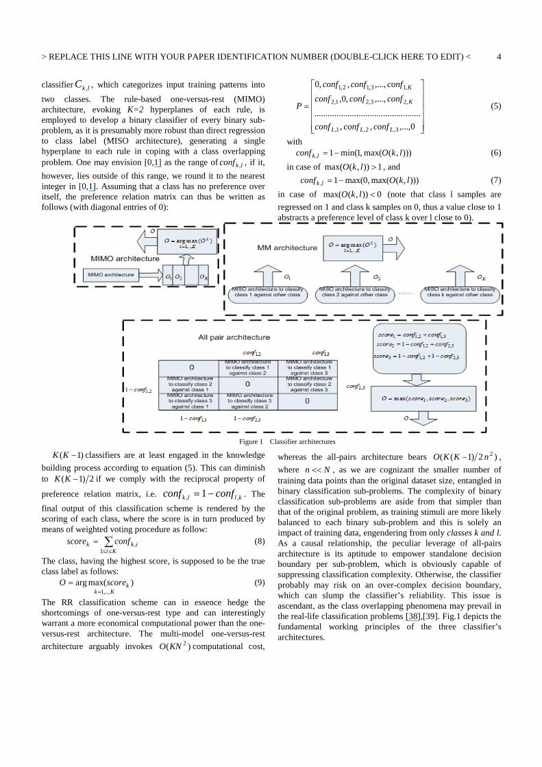
A. MIMO-pClass (rule-based one-versus-rest) The pillar of this architecture [30] is rule consequents,

carrying out a mapping from input features to class labels, where the consequent constitutes a first order polynomial (hyper-plane) for each class. Another landmark in this architecture is a transformation of true class labels to either 0 or 1 value. For instance: if the target class is 2 and the number of class is 2, it should be converted as ]1,0[ . If the input

features fall to Class #3 and the number of class is 3, we modify the true class labels to ]1,0,0[ . The learning on such

labelled data is known as regression by indicator matrix, making up a one-versus-rest regression-based classifier. As we extrapolate the decision boundary, via multiple linear regression models per rule separately (all rules contain K hyper-planes for the K classes), a rule-based one-versus-rest fuzzy classifier is crafted, providing an indicator-based regression for each local region. Each consequent in each rule is thus supposed to learn the respective target class in the local region that the rule represents. In this sense, MIMO architecture is concocted to achieve a more accurate

representation of decision boundaries than classical one-versus-rest approach in regions, where classes overlap.

Furthermore, a one-versus-rest classifier is more convenient to be applied, notably in multiclass classification problems, as direct regression on class labels may suffer severely from over-complex decision boundaries (see e.g. [38]). Apart from that, the TSK fuzzy structure inevitably resorts to predict the decision boundary in a smooth way. If an abrupt changing on class labels from one class to another class (i.e. Class #1 to Class #3) ensues, direct regression to class labels will dispatch a misclassification (i.e. Class #2 will be pointed out). The final classification decision is elicited as the class, which achieves a maximal activation degree over all rules as follow:

)(maxarg,..,1

k

KkOO

=

= (3)

B. Multi Model (MM)-pClass (model-based one-versus-rest) The construct of this architecture is to split multiclass

classification problem into K binary sub-problems on a model level, dubbed the classical one-versus-rest architecture. K Multi-Input-Single-Output (MISO) classifiers are generated with the help of K indicator matrix. This architecture is presumed to have a less flexibility in overlapping class regions than rule-based one-versus-rest approach.

This architecture, nonetheless, can incur costly computational effort and can evoke high system memory, especially if the number of classes and the degree of non-linearity of the decision boundary are high (requiring a high number of rules for each sub-model). Quadratic computational

complexity can be on the one hand imposed )( 2KNO [38]

where N is the total number of training data, as every sub-problem solicits identical number of training data to original problem. The resultant rule base burden is on the other hand a summation of independent rule base burdens, harming the memory demand in the case of an oversized rule base. The final classification decision in form of class O is composed by:

)(maxarg,..,1

k

KkOO

=

= (4)

with kO the regression output of the MISO TS fuzzy model for class K. In addition, both, MIMO and MM architectures may suffer from imbalanced learning problems (one-class is usually under-represented compared to the sum of all other classes). All-pairs architecture is consequently devised to compensate this shortcoming.

C. All-Pairs(AP)-pClass Round Robin (RR) aka all pairs classification scheme

[38],[39] is a plausible alternative to previous two architectures. This classifier architecture relies on all-pairs of target classes to construct binary sub-problems, stemming from a multiclass classification problem. Each sub-problem yields a confidence degree lkconf , , which is summarized in the

preference relation matrix. A confidence degree implies a preference level of class k over class l and the preference relation matrix is formulated by equation (5). The confidence degree lkconf , itself is gained from the output of the

> REPLACE THIS LINE WITH YOUR PAPER IDENTIFICATION NUMBER (DOUBLE-CLICK HERE TO EDIT) <

4

classifier lkC , , which categorizes input training patterns into

two classes. The rule-based one-versus-rest (MIMO) architecture, evoking K=2 hyperplanes of each rule, is employed to develop a binary classifier of every binary sub-problem, as it is presumably more robust than direct regression to class label (MISO architecture), generating a single hyperplane to each rule in coping with a class overlapping problem. One may envision [0,1] as the range of lkconf , , if it,

however, lies outside of this range, we round it to the nearest integer in [0,1]. Assuming that a class has no preference over itself, the preference relation matrix can thus be written as follows (with diagonal entries of 0):

=

0,...,,,

................................................

,...,,0,

,...,,,0

3,2,1,

,23,21,2

,13,12,1

LLL

K

K

confconfconf

confconfconf

confconfconf

P (5)

with ))),(max(,1min(1, lkOconf lk −= (6)

in case of 1)),(max( >lkO , and

))),(max(,0max(1, lkOconf lk −= (7)

in case of 0)),(max( <lkO (note that class l samples are

regressed on 1 and class k samples on 0, thus a value close to 1 abstracts a preference level of class k over l close to 0).

Figure 1 Classifier architectures

)1( −KK classifiers are at least engaged in the knowledge

building process according to equation (5). This can diminish to 2)1( −KK if we comply with the reciprocal property of

preference relation matrix, i.e. kllk confconf ,, 1−= . The

final output of this classification scheme is rendered by the scoring of each class, where the score is in turn produced by means of weighted voting procedure as follow:

∑≤≤

=

Kiikk confscore

1, (8)

The class, having the highest score, is supposed to be the true class label as follows:

KkkscoreO

,..,1)max(arg

=

= (9)

The RR classification scheme can in essence hedge the shortcomings of one-versus-rest type and can interestingly warrant a more economical computational power than the one-versus-rest architecture. The multi-model one-versus-rest

architecture arguably invokes )( 2KNO computational cost,

whereas the all-pairs architecture bears )2)1(( 2nKKO − ,

where Nn << , as we are cognizant the smaller number of training data points than the original dataset size, entangled in binary classification sub-problems. The complexity of binary classification sub-problems are aside from that simpler than that of the original problem, as training stimuli are more likely balanced to each binary sub-problem and this is solely an impact of training data, engendering from only classes k and l. As a causal relationship, the peculiar leverage of all-pairs architecture is its aptitude to empower standalone decision boundary per sub-problem, which is obviously capable of suppressing classification complexity. Otherwise, the classifier probably may risk on an over-complex decision boundary, which can slump the classifier’s reliability. This issue is ascendant, as the class overlapping phenomena may prevail in the real-life classification problems [38],[39]. Fig.1 depicts the fundamental working principles of the three classifier’s architectures.

> REPLACE THIS LINE WITH YOUR PAPER IDENTIFICATION NUMBER (DOUBLE-CLICK HERE TO EDIT) <

5

III. ALGORITHMIC DEVELOPMENT OF PCLASS A. Rule generation via data quality

Automatic knowledge discovery from streaming data of pClass is undertaken by the so-called data quality concept. The data quality paradigm, introduced in this paper, resorts to manifest two dual goals, where the knowledge, offering good summarization power and generalization potential in both of current and future data distributions, is a major subject of investigation.This rule growing adornment, to this end, probes the possible contribution of data in the future, benefiting from approximations of their statistical contributions. The mathematical expression of this method can be for brevity written according to [17],[20] as follows:

∑+=

+=

1

1

1R

ii

Rn

V

VQ (10)

where 1+RV indicates the estimated volume of a hypothetical

new rule (the R+1st). Meanwhile, the expression of nQ can be

observed from the following equation.

dxXSCXCX

XXXXQ

X iii

NRNn )(

1)

)()(

)()((

1

11∫ −∑−

−∑−=−

−+ (11)

where NX and )(XS denote the current data point and size of

the range X respectively. Note that )(XS stems from the

sampling density function )(xl , when the training data are

uniformly distributed, we can define

)(

1)(

XSxl = where ∫=

X

dxXS 1)( . Applying P-fold numerical

integration, we can arrive in the same expression of equation (10) (see also [20]). To circumvent a laborious pre-training process to choose an optimum value of predefined parameters, we heuristically set the condition of the rule generation as follows:

RiiR VV

,...,11 )max(

=+ ≥ (12)

If equation (12) is satisfied, the datum owns a good generalization potential due to a sufficient coverage span, thus crafting it as an extraneous fuzzy rule (it becomes the real R+1st rule).The foundation of this strategy supports to flourish the clusters with a high generalization potential. It can be perceived with the use of the cluster volume to proliferate an extraneous cluster. A cluster, holding high volume, on the one hand, implies a good coverage span to capture the data points. On the other hand, completeness in encompassing feature space in turn navigates to intensify pClass generalization.

This method, solely, makes sense when the training samples are uniformly distributed [33], but imposing many needless clusters evolved, as it does not take into account the data distribution or data history and is regardless of spatial proximity between training samples. The type of data distribution is deemed unfathomable prior to the training process, alongside probable shift, drift in the data streams. Outliers can be, moreover, existent in real-world systems due to a noisy characteristic of the training samples and so the training samples can be imbalanced.

This technical flaw was postulated in [33] where the breakthrough of this bottleneck was lodged, albeit employing a sliding window technique, maintaining some preceding training signals in the memory. This indeed precludes its viability in the limited computational resource circumstance, as the size of sliding window can be possibly very large, notably in confronting a complex classification problem. Another cursor in breeding the fuzzy rules should be devised, where the crux is to supply the summarization power of a newly created cluster. This purpose can be certainly sorted out, enumerating the matching factor or firing strength of the (potential, R+1st) new cluster (rule) against all training samples, observed so far, but with the absence of preceding training stimuli to be salvaged in the memory. In other words, the crux of the Recursive Density Estimation (RDE) method of [16] is taken place to tailor a newly proposed rule growing scenario, termed Extended RDE (ERDE) method as the supplementary cursor of the fuzzy rule generation, in order to hinder the aforementioned drawbacks. Nonetheless, the RDE concept should be carefully implemented, as has been observed in [40], where a large pair-wise distance can be compelled to training samples injected subsequent to noisy training samples or outliers, diminishing the quality of existing clusters. We should weight the distance measure with the quality of the previous sample. We end up with the final expression of the RDE method as follow:

NNNN

NN

n NNNNN

Nin cbaU

U

cbaUU

U

+−+=

+−+=∑−

=2)1(2

1

1

ϕ

(13)

where iN

iN

iN UU 11 −−

+= ϕ TiiiN CCa 1−∑= ,

Nii

NN Cb αϕ 1−= , TNiNN X 1

11 −

−

−Σ+=αα

11

111 −

−

−−−∑+= NiN

iNNN XXcc ϕ .

Furthermore, we amalgamate the so-called condition A in accordance with eTS+ of [41], in order to deter the detrimental effect of predefined parameter selections as follows:

∑ ∑ ∑∑−

==

−

=

−

==

+−

=

+ ≤≥1

1,...,1

1

1

1

1,..,1

11

1

1 )(min)max(N

nRi

N

n

in

N

nRi

Rn

N

n

in

Rn or ϕϕϕϕ (14)

This condition beckons that the datum is either more adjacent than the existing rules to the already seen data clouds or in a region, which is not covered by any of the existing rules. This strategy is efficacious to trace the footprints of training data, as it is delved from the distances of cluster focal-points to all training samples, while abolishing preceding training stimuli to be restrained in the memory. One can be

cognizant the condition ∑ ∑−

=

−

==

+ ≤1

1

1

1,..,1

1 )(minN

n

in

N

nRi

Rn ϕϕ , presiding

to an incorrect provision in generating outliers to be fuzzy rules, as outliers are usually situated in the remote areas, thus yielding low values of data quality. This condition is conversely capable of hinting abrupt or smooth changes of system characteristics, advocating to embed in the rule base the training data, dwelled beyond the zones of influences of the existing fuzzy rules. The drawback against outliers can be

> REPLACE THIS LINE WITH YOUR PAPER IDENTIFICATION NUMBER (DOUBLE-CLICK HERE TO EDIT) <

6

addressed with the use of the rule pruning leverage elaborated in the next section, where the rules, which are superflous during their lifespan, can be trimmed in order to salvage the rule base parsimony and compactness.

The volume of cluster or fuzzy region prevails in the input space partitions with hindsight of two rule growing scenarios, where it is in line with the concept of completeness. We should nevertheless take into account the cluster de-lamination phenomenon [42], weakening the rule semantic and degenerating the classifier’s accuracy. This fact entails us to confine the cluster sizes, in order to in turn evade the cluster de-lamination paradigm, as one cluster can cover two or more data clouds and the first two rule growing scenarios cannot inhibit clusters to culminate uncontrollably.

The size of winning cluster necessitates to be monitored in every training observation, assuring its moderate volume. This idea is coincident with Bayesian Adaptive Resonance Theory (BART) [43] and the so-called GART+ in our past work [20], affirming a demand of limited in size fuzzy regions, so as to allow proper input space granulation. The winning cluster

indexed bywin is sought in accord with the construct of

Bayesian posterior probability as follow:

)(ˆ)|(ˆ)(maxarg ,...,1 iiiRi PXpXPwin ϕϕϕ == =

)

(15)

where )(ˆ iXp ϕ and )(ˆ iP ϕ label the likelihood and prior

probability respectively, where they can be outlined by the following mathematical expression:

))()(exp()2(

1)(ˆ 1

212

1T

iii

i

i CXCXV

XP −Σ−−= −

πϕ (16)

∑=

+

+=

K

kki

kii

N

NP

1,

,

)1log(

)1log()(ˆ ϕ (17)

where iN shows the support of the i-th cluster (rule), which

supplies us a kind of density information, how many samples forming the cluster in the past. Meanwhile,kiN , denotes the

number of supports of the i-th cluster falling into the k-th class. The advantage of Bayesian concept in pinpointing the winning cluster over a pure distance-based concept is a more accurate representation of the winning cluster, paying attention to the number of samples occupying i-th cluster. This is in line with the reality, where two clusters can reside in almost the same proximity to the datum: in this case, the Bayesian concept chooses a cluster supported by more training samples, increasing its likelihood to become the winner. Note that (17) is an enhanced version of prior probability definition of [20], where the prior probability formula is softened. This amendment is aimed to intensify the likelihood of less populated clusters to undergo the resonance and develop their shapes. iV is thereafter calculated as the estimated hyper-

volume of i-th fuzzy rule, which can be defined for ellipsoids in the arbitrary position as follows:

)2/(

*)/(*21

2/

p

rV

p

j

piji

i Γ=∏ =

πλ (18)

with ir the Mahalnobis distance radius of the i-th fuzzy rule,

which defines its (inner) contour (default set to 1) , ijλ the j-th

eigenvalue of the i-th fuzzy rule and Γ the gamma function defined by

dxexp xp∫∞ −−=Γ0

1)( (19)

To expedite the computation of (19), a look-up table can be beforehand generated and used during on-line learning for the actual dimensionality p in the current data set. In a nutshell, the fuzzy rule interpolation is deemed necessary, when the training observation accords with the following condition.

∑=

≥R

iiwin VV

13ρ (20)

where 3ρ stands for a predefined constant, governing the

maximum limit of cluster volume. We allocate this parameter in the range of [0.1,0.5]. The rationale of this parameter setting is as follows: a higher value assigned to this parameter features a more compact and parsimonious rule base produced, this, nonetheless, deteriorates the classification accuracy. Vice versa, a smaller value, opted to this parameter, ameliorates the predictive accuracy, albeit consuming a costlier structural load. A plausible choice is indeed the value, underpinning a trade-off between accuracy and simplicity. We tabulate the pClass experimental results, where3ρ is varied in this range,

exploiting iris dataset [50], in order to amplify the validity of [0.1,0.5] as a sensible option of 3ρ . The data proportion is

70:30 for training and testing respectively and we specify 3ρ

as [0.1,0.3,0.4,0.5]. The predefined constant3ρ can be opted in

this range referring to Table 1, thus warranting to select 3ρ in

[0.1,0.5] as their emphasis between accuracy or simplicity. Table.1. Consolidated performances of pClass varying 3ρ

1.03 =ρ 3.03 =ρ 4.03 =ρ 5.03 =ρ

( rule, acc) (3,1) (2,0.99) (2,0.96) (1,0.95)

As an alternative, one may envision the cluster split technique to obviate the cluster delamination situation in [42]. This strategy is usually carried out with a trial-and-error fashion, where the quality of cluster partition, after halving the cluster size, is scrutinized. This method is, however, very intuitive, where this technique confronts a precarious challenge to maintain a proper input space partition, as the real world data distribution is usually not smooth and two data clouds dwelling one cluster can be imbalanced. It is uneasy to be arranged to simply halve one cluster into two clusters.

Equation (13) is arguably similar with eTS family [16] and the recursive density estimation in [44], [45]. We, in conjunction with this issue, contend that three differences are still at hand. We exploit the non-diagonal covariance matrix for generalized rule antecedents in lieu of the spherical clusters and inverse multi-quadratic function instead of Cauchy function. Furthermore, this rule growing strategy is not standalone to orchestrate the fuzzy rule recruitment. Note that, the computational cost depleted by these rule growing strategies is yet affordable )3( RO , notwithstanding adopting

> REPLACE THIS LINE WITH YOUR PAPER IDENTIFICATION NUMBER (DOUBLE-CLICK HERE TO EDIT) <

7

three different cursors to automate fuzzy rule recruitments. The memory complexities of these rule growing modules are very low which is in the order of )1(O mainly endured by a

recursive calculation of equation (13). B. Initialization of a Newly Born Fuzzy Rule and Premise Part Adaptation

Allocation of a new fuzzy rule parameter ought to be carried out after satisfying all criteria to work up an extraneous fuzzy rule. This step should be carefully plotted, so that a new cluster leads to a favorable input space partition. On the one hand, the datum is amalgamated as a cluster focal point, whereas covariance matrix is stitched up as follows:

NR XC =+1 (21)

distdistcxdist TRjij

pij =∑−= +

=1,

,..,1),(min (22)

Note that the initialization of covariance matrix in equation (22) is different with our works [17]-[20], where the new covariance matrix is set as a diagonal covariance matrix, meaning that the initial contour and shape of the new cluster is the ellipsoidal cluster in the main position. After populated by training exemplars, this cluster initiates to spin, evoked by premise parameter adaptation in equations (25-27). The allocation of covariance matrix, presented herein directly, incurs exact shape and contour of non-axis parallel ellipsoidal clusters, even prior to obtain premise parameter adaptations. On the other side, the output parameters and covariance matrix are plugged in as follows:

winnerR WW =+1 (23)

IR ω=Ψ +1 (24)

where )1()1(1

+×++ ℜ∈Ψ PP

R stands for the inverse covariance

matrix of the output fuzzy rule and the constantϖ is set up as a positive big value. The consequent of the nearest rule is selected as a new rule consequent as the winning rule is expected to delineate a similar trend of the new rule. It is worth-noting that pClass benefits from the concept of local learning scheme [26] with the aid of the so-called Fuzzily Weighted Generalized Least Square (FWGRLS). The noteworthy pillar in local learning is capable of polishing up the fuzzy rule consequents separately, so that the impacts of fuzzy rule growing and pruning do not jeopardize the convergence of existing fuzzy rules. In addition, the strategy of fixing new output covariance matrix is a desirable one, as it can encourage the optimization of FWGRLS, so as to closely forge the real solution using a batched learning scheme [26]. C. Rule Base Simplification C.1 Rule pruning procedure

The similar ideas, as utilized in rule growing components, are adopted in this module. We, first of all, vet the statistical contribution of fuzzy rules in order to oversee fuzzy rule contributions in the future and inspect the position of fuzzy rules in the feature space afterward, whether or not the fuzzy rules are located in the valuable zones according to data distributions. The first objective can be achieved by simply quantifying the following equation.

PR

ii

Pi

P

p

kipi

V

Vy

∑∑

=

+

=

=

1

1

1

β (28)

where iV stands for the volume of i-th rule obtained by

equation (19), thus representing the contribution of input part of the i-th rule, whereas ipy constitutes a hyperplane of i-th

fuzzy rule and in the case of MIMO

architecture ∑=

=

K

k

kipip yy

1

pointing out the total contribution

of output part of i-th fuzzy rule. iβ denotes the statistical

contribution of fuzzy rules and is derived in the tantamount way of equation (10).

If σβββ −< ˆi , where σββ ,ˆ are the average and standard

deviation of fuzzy rule statistical contributions, the fuzzy rule looms to the classifier’s output during its lifespan, it can be pruned without a significant loss of accuracy. This avenue is expedient to that, a cluster, having a light volume, just snapshots a tiny zone in the feature space and a cluster, exploiting a small weight vector y, does not influence the calculation of classifier’s output too much. The forecasting accuracy of superfluous fuzzy rules, exploiting this approach is still debatable, as equation (28) stems from the assumption of uniformly distributed training data. This formula just engages the cluster zone of influence and output parameters to unveil the significances of the fuzzy rules and does not take into account the spatial and temporal proximity of the fuzzy rules to other training samples. It is incapable of pinpointing the cluster, which is not laid on the strategic position of feature space. This method cannot consequently discover the fuzzy rules, which are outdated and obsolete with respect to shift or drift in the data trends.

The later goal is doable with the use of fuzzy rule potential [46]. The key idea is to reflect, whether the fuzzy rules are located in the appropriate positions with respect to the up-to-date data distribution. This method is fruitful not only to seize inactive fuzzy rules, but also to discover obsolete or outdated fuzzy rules, which are no longer relevant to capture the current data trends (e.g, due to shifts). Low potential is clearly yielded to the rules, which reside in the far zone to the recently observed training samples, whereas pivotal clusters, situated in dense regions or dwelled with many training patterns, conversely land on a high value. We can obtain the expression of fuzzy rule contribution as follows:

niininin

ini

dNN

N2

,12

,12

,1

2,1

)1)(2()1(

)1(

−−−

−

+−−+−

−=

χχχ

χχ (29)

where iχ labels the potential of the i-th fuzzy rule whereas nid

epitomizes the Malanobis distance between i-th rule to the newest datum. One can arrive in equation (29), following the same mathematical derivations of [46]. If σχχχ −< ˆi , where

σχχ ,ˆ stand for the average and standard deviation of fuzzy

rule contributions, the fuzzy rules can be subsumed as obsolete fuzzy rules. Hence, the fuzzy rule can be temporarily

> REPLACE THIS LINE WITH YOUR PAPER IDENTIFICATION NUMBER (DOUBLE-CLICK HERE TO EDIT) <

8

deactivated without catastrophic effect of classification accuracy, but can be regenerated in the future subject to the rule recall mechanism condition, deliberated in the next sub-section. One may contemplate the distinct facet of this potential measure with those in eTS family or the rule pruning in [46]. The salient notion of our method is the use of inverse multi-quadratic function in lieu of Cauchy function and the potential measure is exacerbated to endorse the non-axis parallel ellipsoidal clusters driven by the generalized fuzzy

rules. We also refurbish the so-called potential measure to find out inconsequential knowledge (pruning), whereas eTS family adopts it to accomplish an automatic knowledge discovery. We affirm the light computational burden and low memory demand of this method, where it burdens )2( RO as

computational load and )(RO as memory demand to the

system.

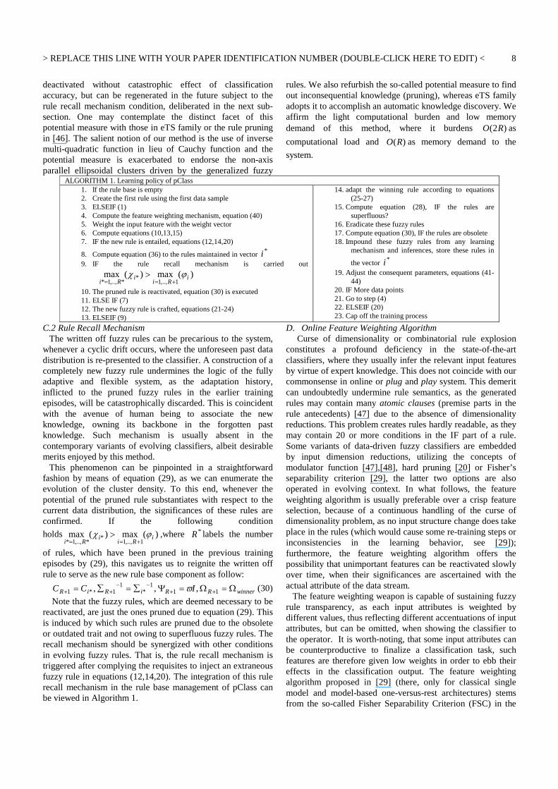
ALGORITHM 1. Learning policy of pClass 1. If the rule base is empty 2. Create the first rule using the first data sample 3. ELSEIF (1) 4. Compute the feature weighting mechanism, equation (40) 5. Weight the input feature with the weight vector 6. Compute equations (10,13,15) 7. IF the new rule is entailed, equations (12,14,20)

8. Compute equation (36) to the rules maintained in vector *i 9. IF the rule recall mechanism is carried out

)(max)(max1,..,1

**,..,1*

iRi

iRi

ϕχ+==

>

10. The pruned rule is reactivated, equation (30) is executed 11. ELSE IF (7) 12. The new fuzzy rule is crafted, equations (21-24) 13. ELSEIF (9)

14. adapt the winning rule according to equations (25-27)

15. Compute equation (28), IF the rules are superfluous?

16. Eradicate these fuzzy rules 17. Compute equation (30), IF the rules are obsolete 18. Impound these fuzzy rules from any learning

mechanism and inferences, store these rules in

the vector *i 19. Adjust the consequent parameters, equations (41-

44) 20. IF More data points 21. Go to step (4) 22. ELSEIF (20) 23. Cap off the training process

C.2 Rule Recall Mechanism The written off fuzzy rules can be precarious to the system,

whenever a cyclic drift occurs, where the unforeseen past data distribution is re-presented to the classifier. A construction of a completely new fuzzy rule undermines the logic of the fully adaptive and flexible system, as the adaptation history, inflicted to the pruned fuzzy rules in the earlier training episodes, will be catastrophically discarded. This is coincident with the avenue of human being to associate the new knowledge, owning its backbone in the forgotten past knowledge. Such mechanism is usually absent in the contemporary variants of evolving classifiers, albeit desirable merits enjoyed by this method.

This phenomenon can be pinpointed in a straightforward fashion by means of equation (29), as we can enumerate the evolution of the cluster density. To this end, whenever the potential of the pruned rule substantiates with respect to the current data distribution, the significances of these rules are confirmed. If the following condition

holds )(max)(max1,..,1

**,..,1*

iRi

iRi

ϕχ+==

> ,where *R labels the number

of rules, which have been pruned in the previous training episodes by (29), this navigates us to reignite the written off rule to serve as the new rule base component as follow:

winnerRRiRiR ICC Ω=Ω=Ψ∑=∑= ++−−

++ 111

*1

1*1 ,,, ϖ (30)

Note that the fuzzy rules, which are deemed necessary to be reactivated, are just the ones pruned due to equation (29). This is induced by which such rules are pruned due to the obsolete or outdated trait and not owing to superfluous fuzzy rules. The recall mechanism should be synergized with other conditions in evolving fuzzy rules. That is, the rule recall mechanism is triggered after complying the requisites to inject an extraneous fuzzy rule in equations (12,14,20). The integration of this rule recall mechanism in the rule base management of pClass can be viewed in Algorithm 1.

D. Online Feature Weighting Algorithm Curse of dimensionality or combinatorial rule explosion

constitutes a profound deficiency in the state-of-the-art classifiers, where they usually infer the relevant input features by virtue of expert knowledge. This does not coincide with our commonsense in online or plug and play system. This demerit can undoubtedly undermine rule semantics, as the generated rules may contain many atomic clauses (premise parts in the rule antecedents) [47] due to the absence of dimensionality reductions. This problem creates rules hardly readable, as they may contain 20 or more conditions in the IF part of a rule. Some variants of data-driven fuzzy classifiers are embedded by input dimension reductions, utilizing the concepts of modulator function [47],[48], hard pruning [20] or Fisher’s separability criterion [29], the latter two options are also operated in evolving context. In what follows, the feature weighting algorithm is usually preferable over a crisp feature selection, because of a continuous handling of the curse of dimensionality problem, as no input structure change does take place in the rules (which would cause some re-training steps or inconsistencies in the learning behavior, see [29]); furthermore, the feature weighting algorithm offers the possibility that unimportant features can be reactivated slowly over time, when their significances are ascertained with the actual attribute of the data stream.

The feature weighting weapon is capable of sustaining fuzzy rule transparency, as each input attributes is weighted by different values, thus reflecting different accentuations of input attributes, but can be omitted, when showing the classifier to the operator. It is worth-noting, that some input attributes can be counterproductive to finalize a classification task, such features are therefore given low weights in order to ebb their effects in the classification output. The feature weighting algorithm proposed in [29] (there, only for classical single model and model-based one-versus-rest architectures) stems from the so-called Fisher Separability Criterion (FSC) in the

> REPLACE THIS LINE WITH YOUR PAPER IDENTIFICATION NUMBER (DOUBLE-CLICK HERE TO EDIT) <

9

original feature space. In this paper, we go a step further, extending the feature weighting approach, as introduced in [29], to the empirical feature space, utilizing the kernel trick [34],[35], retaining the geometrical structure of training data. The separability criterion is easier to be evaluated in the empirical feature space than in the original feature space, consequently affecting its run-time performance. The within-class-scatter-matrix and between-class-scatter-matrix wb SS , expressions can be then expressed as follows:

∑ ∑−= KN

WStr b

1)( (31)

∑−= WKtrStr w )()( (32)

Note that the symbol WΣ means the sum of matrix W in every

dimension∑ji

W,

.

KiNKdiagN

W iii ,...,1),/(1

== (33)

=

KKKkKK

Kk

Kk

KKKK

KKKK

KKKK

K

,..,,..,,

....................................

,..,,..,,

,..,,..,,

21

222221

111211

(34)

where K represents a kernel-Gram-matrix. One may

comprehend, that 1111

NNK ×ℜ∈ signifies a kernel-Gram-sub-

matrix, emanating from data in class 1,

whereas 2112

NNK ×ℜ∈ constitutes a kernel-Gram-sub-matrix,

originating from data in class 1 and 2 and so on. The kernel class separability is then gauged as follows:

∑∑ ∑

−

−

=WKtr

NK

WJ

)( (35)

Assuming that the Gaussian kernel is used, the element of

kernel-Gram-matrix (for class-pair )ˆ,( kk ) is enumerated as

follows:

))()(exp( 1ˆ

jk

ikkk

jk

ik

ijkk

XXXXK ))) −∑−−= − (36)

where the indices i,j stand for the i or j-th training sample and i

kX exhibits the i-th training sample of k-th class. This

method is obviously compatible in the offline learning scenario wherein all training samples are accessible before this process can commence to act. Gaussian kernel is in addition unable to endorse a recursive calculation, thus impending the incremental learning. Our contribution herein is to suit the FSC in the empirical feature space to the online learning platform. We accordingly borrow the construct of Angelov [28] to a recursive version of Cauchy kernel:

NNN

Nkk N

NK ςθϑ 2)1)(1(

)1(ˆ

−++−

−= (37)

where ∑=

=

P

p

kpN Nx

1

2))((ϑ , ∑=

− −+=P

p

kpNN Nx

1

2ˆ1 ))1((θθ

∑=

=

P

pN

kpN Nx

1

)( νς , kNNN x

ˆ11 −−

+=νν . kp Nx )( is the p-th

element of the N-th training sample falling into class k. 0θ and

0ν can be initialized as zero before the process runs. This

Cauchy kernel constitutes a Taylor series approximation of Gaussian function and more importantly leads to a possible recursive computation: adapting (37) for all class pairs, automatically yields (31), (32) and hence (35) in incremental learning context.

Weights of input features are defined through Leave-One-Feature-Out (LOFO) approach [29]. The major ingredient of this technique is to figure out the class separability J in equation (37) P times ],...,,[ 21 PJJJJ = . Whenever a

measurement of the class separability is undertaken, one input attribute is masked. This is intended to conceive the discrimination power of each input attribute, where the input weights are then enacted as follows:

)(min)(max

)(min1

,..,1,..,1

,..,1

pPp

pPp

pPp

p

p JJ

JJ

==

=

−

−

−=λ (38)

Essentially, each feature weight is normalized to [0,1] and

a feature p with a high value of pJ gains a low weight, as it

has been left out and still a high value remains meaning that the change in discriminatory power is marginal, thus being able to judge as inconsequential features. The input weight vector is later on consolidated in the inference and learning scheme as follows:

)))(*.())(*.(exp( 1,

Tiniinwi CXCX −∑−−= − λλϕ (39)

Furthermore, the input weighting scheme will also be used in the training and evolution engine of pClass: in all distance calculations, in all calculations, involving solely the covariance or inverse covariance matrix. This is prone to apply, as it is the same as (39). The output part is indeed affected by this input weighting technique, notwithstanding taken place in the premise part due to consequent adaptations. The rationale of the use of LOFO approach rather than Single dimension-wise (SD) [29] approach is that it provides a much better approximation of the discriminatory power of single features, as the decrease along all remaining ones is measured. LOFO approach, still and all, costs heavier computational

burden in the order of )( 22PKO whereas SD approach burns

into )(PO computational overhead. Meanwhile, the memory

complexity is approximated around )( 22 PKPO + . This

assumption holds if the evaluation of class separability is enforced in the feature space. The complexity can be mitigated with the use of the class separability in the empirical feature space, as within class scatter and between class scatter matrices do not attract adaptations in every training observation, solely necessitating the kernel-gram matrix to be carved out, thus incurring the computational complexity in the

> REPLACE THIS LINE WITH YOUR PAPER IDENTIFICATION NUMBER (DOUBLE-CLICK HERE TO EDIT) <

10

order of )( 2KPO . Apart from that, this ingredient truncates

the memory complexity to the order of )(KO .

To pry the efficacy of our proposed learning module, we compare the online feature weighting algorithm, benefiting from Fisher’s separability criterion in the feature space [29], in the empirical feature space, postulated in this paper, and without feature weighting algorithm, benefiting from three problems, namely spam base, ionosphere emanating from University of California, Irvine (UCI) machine learning repository [51] and food production (supervision of eggs) [29]. All numerical results are granted by means of 10-folds cross-validation method (evolving the models on 9 out of 10 folds) and classical MIMO architecture is in charge as a classifier inference scheme. Table 2 summarizes the consolidated experimental results of three learning configurations.

Clearly, the feature weighting-based empirical feature space devolves more accurate classification rates than those of the feature weighting-based feature space and no feature weighting with the same sensitivity on the various folds. Regarding computation times, the improvement is major, when using the new feature weighting approach in the empirical feature space, as the update of the within-class scatter matrix and between-class scatter matrix is not operated, which is deemed to cost a considerable computational load.

Table 2. Comparisons between two feature weighting schemes Algorithms Spam base Ionosphere Eggs Empirical feature space

Classification rate

0.9±0.02 0.82±0.18 0.93±0.06

Rule 2.1±0.05 2.8±0.19 3±1.33 Time 19.5±3.3 0.15±0.02 4.73±0.33

Feature space Classification rate

0.89±0.02 0.82±0.19 0.92±0.05

Rule 2.1±0.05 2.8±1.48 3±1.33 Time 279.15±3.4

9 0.72±0.08 55.45±2.2

6 No feature weighting

Classification rate

0.87±0.01 0.81±0.15 0.9±0.03

Rule 2.1±0.05 2.8±1.48 2.22±0.6 Time 7.11±0.16 0.06±0.01 3±1.33

A. Adaptation of Consequent Parameters pClass algorithm makes use of Fuzzily Weighted

Generalized Least Square (FWGRLS) method of [20], developed from Fuzzily Weighted Recursive least Square (FWRLS) theory to fine tune fuzzy rule consequents. Some prominent works of the RLS method were proposed in [49],[50]. The FWGRLS method is motivated by Generalized Recursive Least Square (GRLS) [37], we, yet, conform it in the local learning context, in order to achieve better flexibility, a higher robustness etc. [26]. The crux of FWGRLS method synergizes the local learning concept and the weight decay term in the adaptation scheme. The weight decay term is useful to decay the consequents, thus hovering around the small bounded values. This improvement confers better generalization ability and is by extension worthwhile to induce a more compact and parsimonious rule base. As the weight vectors fluctuate in the small values, inactive fuzzy rules usually own very small weights and then can be pruned to mitigate structural burden by virtue of equations (27). We set off from the new definition of the energy function as follow:

∑=

−

−

−−+

Ω+−−=Ω

n

n

T

iynyPyny

nnyntnRnyntE

11

0

1

)))0()(())0()((

))((2))()(()())()((()(

ϖξ (40)

where )1()1()( +××ℜ∈ ppnR stands for a covariance matrix of

modelling error and ))(( nΩξ labels the genaralized decay

function. There are two salient facets of this energy function in contrast with the standard energy function of Recursive Least Square (RLS) method, which constitute the covariance matrix of modelling error and the generalized decay function. The covariance matrix of modelling error induces more realistic assumption notably, when the output of each local sub-system possesses different statistical properties. A generalized weight decay regularizer can contain any weight decay functions, enabling to suit with more general training cases. Following with the same mathematical derivations of [26], we can arrive in the mathematical expression of FWGRLS method as follows:

1))()1()()(

)()(()1()( −−Ψ+Λ

−Ψ= nFnnFn

nRnFnn T

ii

iψ (41)

)1()()()1()( −Ψ−−Ψ=Ψ nnFnnn iii ψ (42)

))()()((

))1(()()1()(

nyntn

nnnn iiii

−Ψ+−Ω∇Ψ−−Ω=Ω ξϖ

(43)

)()( nxny ienΩ= and enxn

nynF =

Ω∂∂=

)(

)()( (44)

where )1()1()( ××+ℜ∈Λ PPi n denotes a diagonal matrix, whose

diagonal elements comprise iϕ and the covariance matrix of

modelling error )(nR is set to an identity matrix as its default in

[26]. Meanwhile, ϖ represents a predefined constant whose

default value 1510−

≈ϖ and ))1(( −Ω∇ niξ stands for a

gradient of a weight decay function. Note that the generalized weight decay function can be stipulated as any non-linear functions, in which no exact solution to it can be obtained. As breakthrough, )( iΩ∇ξ can be therefore expanded at n-

1 ))1(( −Ω∇ niξ .

There are four weight decay functions, which are omnipresent in the current literature involving constant, quadratic, quartic, multimodal weight decay functions. We choose the most eminent one, which is the quadratic weight decay function as follow:

2))1((2

1))1(( −Ω=− nny iiξ (45)

Its derivative is written as follow )1())1(( −Ω=−∇ nny iiξ (46)

The centric trait of this weight decay function is capable of smoothly shrinking the weight vector values to a factor proportional to its current values.

IV. EMPIRICAL STUDY A. Comparisons of various classifier architectures

This sub-section finds out the efficacy of the classifier’s architectures deliberated in Section II, embracing the MIMO, one-against-all and one-versus-rest architectures and the leverages of the classifier’s architectures in the computational complexity, predictive quality and memory burden of the

> REPLACE THIS LINE WITH YOUR PAPER IDENTIFICATION NUMBER (DOUBLE-CLICK HERE TO EDIT) <

11

classifier are addressed. pClass algorithm is embedded in each classifier architecture to which they are benchmarked in 6 multi-category classification problems, obtained from UCI machine learning repository [51].

The study cases, namely iris, wine, thyroid and image segmentation, are cultivated by virtue of 10-fold Cross Validation (CV) procedure [51]. In the CV procedure, we, firstly, split the complete dataset into 10 mutually exclusive data bins. Henceforth, the first data bin is exploited to quiz the generalization of the classifier, whereas the training process to work out the classifier’s model is embarked with other data bins. The experimental process continues with the second data bin as testing samples, whereas other data bins are injected in the training process to elicit the classifier’s structure. The CV process is terminated, when all data bins have been depleted as testing samples. This CV mechanism is auspicious to avert the data order dependency problem, thus leading to reliable numerical results.

Meanwhile, the numerical results in the shuttle and pen digits datasets are generated with the periodic hold-out process. The periodic hold-out process segregates the dataset into 10 standalone sub-problems, where it commences with the first sub-problem. Every sub-problem pulls out 70% of the total data in each sub-problem to the training process, whereas the rest of data is enacted to assess the classifier’ generalization. The periodic hold-out process is capped off, when experiments with the use of all sub-problems have been undergone. The periodic hold-out process is digestible as a simulation of the training and testing processes in the real-time circumstance. Note that pClass algorithm executes the training samples in the single-pass learning mode. The dataset characteristics are encapsulated by Table 3, including the number of input features, classes and data points.

Table 3. Dataset specifications. datasets Num of input

attributes Num of classes

Num of data points

SEA 3 2 60000 Iris 4 3 150

Wine 13 3 178 Electricity pricing 8 2 45312

Weather Line

Circle Sin Sinh

Boolean Noise corrupted

signal

4 2 2 2 2 3 1

2 2 2 2 2 2 3

60000 2500 2500 2500 2500 1200 100K

Image segmentation

19 7 2310

Spam base 57 2 4601 Shuttle recognition 9 8 14500

Pen digits 16 9 10992 Ionosphere 34 2 351

Egg inspections 57 2 11000

Hyper-planes Thyroid

4 21

2 3

120 K 7200

On the one hand, we quantify the classification rate as the ratio of correctly classified testing samples towards the total samples in the testing process. On the other hand, we gauge the memory efficiency of the classifier with the aid of the total rule base parameters conserved in the memory, where the

pClass rule base parameters in the three different architectures

are fathomed as follows: ))1(( 2 +++ PKRPRRPO (MIMO),

)))1(2(( 2 +++ PRPRRPKO (one versus rest) and

)))1(2)(1(2/( 2 +++− PRPRRPKKO (round robin). By

extension, the training times of the algorithms are so reported, where the specification of computational resources to spark the numerical results is intel (R) core (TM) i7-2600 CPU @3.4 GHz processor and 8 GB memory. The numerical results of consolidated classifiers are organized in Table 4, where the highlighted results of Table 4 are formed as the average results of all sub-problems of the CV or periodic hold-out process.

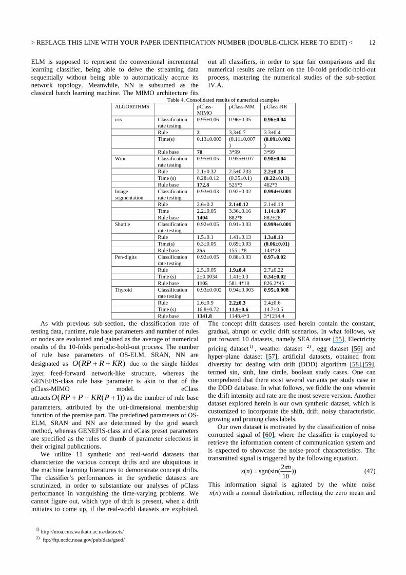
pClass, making use of RR architecture, could outperform the predictive accuracies of other architectures in all study cases. Presumably, the RR architecture can unravel the classification complexities of multi-class classification problems, revamping the complicated multi category classification problems into simpler binary classification problems. This concept sustains to unfold a standalone classification boundary per sub-problems, which can in turn stave off over-complex decision boundaries, as produced by the other two architectures. We allege that over-complex decision boundaries can blunt the predictive accuracy, as spotted in MIMO and MM architectures. As the nature of real-world classification problems can be encroached by the class-overlapping issue, the MIMO and MM architectures essentially do not relieve the classification complexity into independent binary sub-problems. Nonetheless, the MIMO architecture can dispatch better classification results than that of the MM architecture, as the MIMO architecture is mounted with multiple local linear hyper-planes per rule, which may goad to govern one class to other classes and can eventually dodge misclassifications due to class-overlapping phenomena.

The MIMO architecture could bear the costliest computational burden, notwithstanding carried out with the single classifier model. Conversely, the MM and RR architectures break the overall problem into several sub-problems, where every sub-problem is settled by means of a more provident rule base load. The RR architecture could produce swifter training times than that of the MM architecture, as every sub-problem in the RR architecture does not lean on a complete dataset. The MIMO architecture, nevertheless, withstands the most modest memory demand than those of other two architectures, as the total rule base burden of the MM and RR architectures strains the total rule-base burdens of the sub-problems. B. Benchmarks with state-of-the-art classifiers in the concept drift datasets

This subsection is plotted to uphold the precedents of pClass aptitude in handling the learning in the non-stationary environments or concept drifts. In parallel to that, benchmarks with contemporary classifiers are unveiled herein, in order to confirm that pClass is more vigorous than those of other consolidated algorithms to cope with the concept drifts of data streams. We contest pClass against eClass [30], GENEFIS-class [53], SRAN [54], where these algorithms pose a class of evolving classifiers. Other algorithms amalgamated in our numerical studies are NN [2] and OS-ELM [7], where OS-

> REPLACE THIS LINE WITH YOUR PAPER IDENTIFICATION NUMBER (DOUBLE-CLICK HERE TO EDIT) <

12

ELM is supposed to represent the conventional incremental learning classifier, being able to delve the streaming data sequentially without being able to automatically accrue its network topology. Meanwhile, NN is subsumed as the classical batch learning machine. The MIMO architecture fits

out all classifiers, in order to spur fair comparisons and the numerical results are reliant on the 10-fold periodic-hold-out process, mastering the numerical studies of the sub-section IV.A.

Table 4. Consolidated results of numerical examples

ALGORITHMS pClass-MIMO

pClass-MM pClass-RR

iris Classification rate testing

0.95±0.06 0.96±0.05 0.96±0.04

Rule 2 3,3±0.7 3.3±0.4 Time(s) 0.13±0.003 (0.11±0.007

) (0.09±0.002)

Rule base 70 3*99 3*99 Wine Classification

rate testing 0.95±0.05 0.955±0.07 0.98±0.04

Rule 2.1±0.32 2.5±0.233 2.2±0.18 Time (s) 0.28±0.12 (0.35±0.1) (0.22±0.13) Rule base 172.8 525*3 462*3 Image segmentation

Classification rate testing

0.93±0.03 0.92±0.02 0.994±0.001

Rule 2.6±0.2 2.1±0.12 2.1±0.13 Time 2.2±0.05 3.36±0.16 1.14±0.07 Rule base 1404 882*8 882±28 Shuttle Classification

rate testing 0.92±0.05 0.91±0.03 0.999±0.001

Rule 1.5±0.1 1.41±0.13 1.3±0.13 Time(s) 0.3±0.05 0.69±0.03 (0.06±0.01) Rule base 255 155.1*8 143*28 Pen-digits Classification

rate testing 0.92±0.05 0.88±0.03 0.97±0.02

Rule 2.5±0.05 1.9±0.4 2.7±0.22 Time (s) 2±0.0034 1.41±0.3 0.34±0.02 Rule base 1105 581.4*10 826.2*45 Thyroid Classification

rate testing 0.93±0.002 0.94±0.003 0.95±0.008

Rule 2.6±0.9 2.2±0.3 2.4±0.6 Time (s) 16.8±0.72 11.9±0.6 14.7±0.5 Rule base 1341.8 1148.4*3 3*1214.4

As with previous sub-section, the classification rate of testing data, runtime, rule base parameters and number of rules or nodes are evaluated and gained as the average of numerical results of the 10-folds periodic-hold-out process. The number of rule base parameters of OS-ELM, SRAN, NN are designated as )( KRRRPO ++ due to the single hidden

layer feed-forward network-like structure, whereas the GENEFIS-class rule base parameter is akin to that of the pClass-MIMO model. eClass attracts ))1(( +++ PKRPRPO as the number of rule base

parameters, attributed by the uni-dimensional membership function of the premise part. The predefined parameters of OS-ELM, SRAN and NN are determined by the grid search method, whereas GENEFIS-class and eCass preset parameters are specified as the rules of thumb of parameter selections in their original publications.

We utilize 11 synthetic and real-world datasets that characterize the various concept drifts and are ubiquitous in the machine learning literatures to demonstrate concept drifts. The classifier’s performances in the synthetic datasets are scrutinized, in order to substantiate our analyses of pClass performance in vanquishing the time-varying problems. We cannot figure out, which type of drift is present, when a drift initiates to come up, if the real-world datasets are exploited.

The concept drift datasets used herein contain the constant, gradual, abrupt or cyclic drift scenarios. In what follows, we put forward 10 datasets, namely SEA dataset [55], Electricity

pricing dataset)1 , weather dataset )2 , egg dataset [56] and hyper-plane dataset [57], artificial datasets, obtained from diversity for dealing with drift (DDD) algorithm [58],[59], termed sin, sinh, line circle, boolean study cases. One can comprehend that there exist several variants per study case in the DDD database. In what follows, we fiddle the one wherein the drift intensity and rate are the most severe version. Another dataset explored herein is our own synthetic dataset, which is customized to incorporate the shift, drift, noisy characteristic, growing and pruning class labels.

Our own dataset is motivated by the classification of noise corrupted signal of [60], where the classifier is employed to retrieve the information content of communication system and is expected to showcase the noise-proof characteristics. The transmitted signal is triggered by the following equation.

))10

2sgn(sin()(

nns

π= (47)

This information signal is agitated by the white noise )(nn with a normal distribution, reflecting the zero mean and

)1 http://moa.cms.waikato.ac.nz/datasets/ )2 ftp://ftp.ncdc.noaa.gov/pub/data/gsod/

> REPLACE THIS LINE WITH YOUR PAPER IDENTIFICATION NUMBER (DOUBLE-CLICK HERE TO EDIT) <

13

the standard deviation 6.0=nσ . The noise induced signal

)(nsn is expressed as follow:

)()()( nnnsnsn += (48)

Table 5.The consolidated results of benchmarked algorithms ALGORITHMS pClass eClass GENEFIS-class SRAN OS-ELM NN

SEA dataset Classification rate

0.88±0.02 0.87±0.03 0.87±0.001 0.63±0.11 0.61±0.001 0.86±0.03

Rule 2.1±0.74 9.2±2.2 2.9±1 39.7±1 100 100 Time(s) 2.97±0.5 6.1±1.5 3.02±0.26 6.93±0.4 0.006±0.00

8 3.27±0.6

Rule base 42 104.2 58 238.2 600 600 Electricity pricing dataset Classification

rate 0.78±0.05 0.77±0.07 0.75±0.0 0.53±0.07 0.57±0.09 0.53±0.0

8 Rule 3.2±1.2 11.9±0.07 3.5±1.5 37.7±3.1 100 100

Time(s) 0.74±1.01 1.12±2.2 0.49±0.4 5.3±0.4 2.43±0.2 9.61±2.2 Rule base 288 321.3 315 414.7 1100 1100

Sin dataset Classification rate

0.82±0.2 0.81±0.5 0.81±0.2 0.52±0.3 0.8±0.2 0.78±0.18

Rule 3.3±1.2 4±1.14 5.4±2.2 35.8±3.8 50 100 Time(s) 0.15±0.01 0.1±0.02 0.32±0.3 0.17±0.00

1 0.25±0.02 0.66±0.6

3 Rule base 39.6 44 58.8 250.6 500 700

Circle dataset Classification rate

0.73±0.17 0.7±0.11 0.7±0.03 0.7±0.14 0.66±0.14 0.69±0.02

Rule 2.8±1.1 3.6±0.84 3.2±1.03 23.3±5.37 50 800 Time(s) 0.15±0.008 0.09±0.01 0.15±0.01 0.16±0.01 0.08±0.02 6.7±0.8

Rule base 33.6 32.4 38.4 209.7 500 5600 Line dataset Classification

rate 0.91±0.07 0.89±0.06 0.9±0.07 0.79±0.2 0.91±0.08 0.89±0.1

Rule 2.5±0.71 4.4±0.51 3.6±0.7 16.3±0.7 25 200 Time(s) 0.15±0.000

9 0.1±0.009 0.14±0.01 0.12±0.00

6 0.04±0.02 0.82±0.1

2 Rule base 30 39.6 43.2 81.5 250 1400

Sinh dataset Classification rate

0.71±0.09 0.7±0.07 0.71±0.06 0.64±0.3 0.68±0.04 0.69±0.12

Rule 3.6±1.9 6.3±1.5 3.6+0.8 31.8±2.5 50 500 Time(s) 0.17±0.01 0.13±0.02 0.15±0.02 0.2±0.03 0.07±0.02 0.6±0.02

Rule base 43.2 56.7 43.2 286.2 500 3500 Weather dataset Classification

rate 0.8±0.01 0.8±0.05 0.8±0.02 0.63±0.12 0.74±0.06 0.8±0.07

Rule 3.8±2.5 5.6±1.72 4.4±1.64 39±1.8 80 80 Time(s) 1.27±0.18 1.13±0.3 1.13±0.14 1.5±0.1 0.56±0.7 1.4±0.1

Rule base 342 151.2 396 1053 2160 2160 Hyper-plane dataset Classification

rate 0.92±0.02 0.91±0.02 0.91±0.01 0.66±0.09 0.88±0.03 0.91±0.0

9 Rule 2.2±0.63 8.6±2 3.39±0.12 40 35.3±4.16 10

Time(s) 1.86±0.07 13.48±3.61

3.4±0.05 14.3±0.5 1.22±0.13 5.65±0.06

Rule base 66 124.4 90 280 2118 70 Noise corrupted signal

dataset Classification

rate 0.74±0.12 0.72±0.12 0.73±0.09 0.71±1.3 0.72±0.14 0.68±0.3

Rule 3±1.2 3.7±1.3 4.5±1.1 36.4±12.5 50 80 Time(s) 6.4±0.7 6.9±1.9 7.5±0.9 7.64±2.52 2.23±0.11 10.6±0.3

Rule base 24 29.6 36 291.2 400 640 Boolean dataset Classification

rate 0.83±0.2 0.81±0.2 0.82±0.2 0.68±0.35 0.8±0.17 0.8±0.1

Rule 2.6±0.8 3.7±1.1 2.6±1.1 4.8±0.6 100 100 Time (s) 0.08±0.002 0.04±0.01 0.09±0.05 0.01±0.03 0.24±0.02 0.2±0.02 Rule base 52 44.4±12.7 52 28.8±3.8 600 600

Egg dataset Classification rate

0.78±0.1 0.75±0.16 0.76±0.01 0.73±0.07 0.74±0.1 0.66±0.5

Rule 5.3±2.1 16.3±5.5 5.9±5.5 34.2±0.6 50 50 Time(s) 5.47±2.2 5.5±1.2 12.01±18.8 1±0.1 0.3±0.03 19.14±3.

9 Rule base 1813.7 2836.2 2019 2052 3000 3000

To arouse the abrupt changing data distribution, the external disturbance encroaches the system at n=10000 to n=20000. The received signal is then defined as follows:

)()()( nfnsnx += (49)

where the disturbance )(nf actualizes a step signal as follows:

> REPLACE THIS LINE WITH YOUR PAPER IDENTIFICATION NUMBER (DOUBLE-CLICK HERE TO EDIT) <

14

≤≤><=

2000010000,1

20000,10000,0)(

n

nnnf (50)

The demodulator is supposed to categorize the received signal )(nx as class 1 signals, if they fall beneath the

thresholdθ and vice versa. The threshold θ is initially stipulated as 0=θ , subsequently, it is altered to spur the recurrent drift circumstance. The cyclic drift property is sorted out, assigning 1−=θ at 3000020000 <≤ n and

1=θ at 4000030000 <≤ n . Henceforth, a new class 3 is appended in the time period 5000040000 <≤ n to complicate the study case with an addition of a new class. Therefore, the classification problem is amended, where the data are grouped as the class 1, if the samples are below the threshold 1−≤θ , whereas they are classified as class 2 when they fall into the range of 11 <<− θ . If )(nx is higher than the threshold 1>θ ,

we annotate the data to class 3. The classification problem reverts as the binary classification problem, by which the class 2 is ruled out for 50000≥n .

Generally speaking, this dataset not only devolves the abrupt or smooth changing of data distributions, but also goads the dynamic class labels, working up the new class label and eroding the past class label. Apart from that, the dataset can accommodate the inquiry of the noise-proof trait of the classifiers, in which the information signal is corrupted by the Gaussian white noise. )(nx is a sole input feature, guiding to

categorize the training exemplars. The schematic diagram of the classification problem is depicted by Fig.2. The

experimental results of the benchmarked algorithms are encapsulated by Table 5. Fig.3(a) visualizes the fuzzy rule trace in one of 10-fold hold-out processes, exploiting the weather dataset and Fig.3(b) portrays the feature weight evolutions in the 10-fold periodic hold-out process, using weather dataset.

pClass could produce the most encouraging numerical results in terms of the classification rate, number of fuzzy rules, and number of rule base parameters. pClass is, furthermore, capable of outperforming the classification rates of other algorithms in almost all study cases except sinH dataset, where GENEFIS-class and NN could outstrip the predictive accuracy of pClass. The number of fuzzy rules, scattered in the training process, is as with the classification rate, where pClass could tailor the most compact and parsimonious rule bases in 10 out of 11 empirical studies. Interestingly, pClass could incur the most modest memory demand in SEA, electricity pricing, line, hyper-plane, egg and noise corrupted signals datasets, notwithstanding making use of the generalized fuzzy rule type, quibbled to consume a more demanding rule-base burden than the conservative axis-parallel clusters or spherical clusters. In term of runtime, pClass runtimes are comparable with other algorithms, where pClass could land on the second place in SEA, electricity pricing, sin, hyperplane, noise corrupted signals datasets, on the third place in the circle, egg and Boolean datasets and on the fourth place in the weather and line datasets.

Table 6. Classifier ranking according to 4 evaluation criteria Study cases pClass

(CR, R, ET, RB) eClass

(CR, R, ET, RB) GENEFIS-class (CR, R, ET, RB)

SRAN (CR, R, ET, RB)

OS-ELM (CR, R, ET, RB)

NN (CR, R, ET, RB)

Sea dataset (1,1,2,1) (3,3,5,3) (2,2,3,2) (5,4,6,4) (6,6,1,5) (4,6,4,5) Electricity

pricing dataset (1,1,2,1) (2,3,3,3) (3,2,1,2) (4,4,5,4) (5,5,4,5) (6,5,6,5)

Sin dataset (1,1,2,1) (3,2,1,2) (2,3,5,3) (6,4,3,4) (4,5,4,5) (5,6,6,6) Circle dataset (1,1,3,2) (3,3,2,1) (2,2,3,3) (4,4,5,4) (6,5,1,5) (5,6,6,6) Line dataset (1,1,5,1) (4,3,2,2) (3,2,4,3) (6,4,3,4) (2,5,1,6) (5,6,6,6) Sinh dataset (2,2,4,2) (3,3,2,3) (1,1,3,1) (5,4,5,4) (5,5,1,5) (4,6,6,6)

Weather dataset (1,1,5,2) (3,3,3,1) (2,2,2,3) (6,4,6,5) (3,5,1,5) (4,5,5,5) Hyper-plane

dataset (1,1,2,2) (3,3,5,4) (2,2,3,3) (6,6,6,6) (5,5,1,6) (4,3,5,2)

Noise corrupted signal dataset

(1,1,2,1) (3,2,3,2) (2,3,4,3) (5,4,5,4) (4,5,1,5) (6,6,6,6)

Boolean dataset (1,1,3,3) (3,3,2,2) (2,2,4,4) (6,4,1,1) (5,5,6,5) (4,5,5,5) Egg dataset (1,1,3,1) (3,3,4,4) (2,2,5,2) (5,4,2,3) (4,5,1,5) (6,5,6,5)

Average (1.1,1.1,3,1.5) (3,2.8,2.9,2.5) (2.1,2.6,3.4,2.4) (5.3,4.2,4.3,3.9) (4.5,5.1,2,5.2) (4.8,5.4,5.5,5.2) CR=classification rate, R=rule, ET=execution time, RB=rule base

Fig.3(b) visualizes the impact of the feature weighting algorithm, coupled in pClass, where the feature weights, illustrating the input feature significances, fluctuate, hinging on the learning context. The high feature weight, granted a weight around 1, is vetted, as the input attribute supplies the informative guide to resolve the classification problem. However, the input feature could be out-weighted, stipulated with a low weight about zero, smoothly repealing its influence to upgrade the decision boundary and to adapt the fuzzy rules. The rule recall module, as depicted by Fig.3(a), plays a noteworthy role, when the cyclic drift ensues. This learning module uncovers a possibility to revive the already pruned focal points, as the current data trend toughens its relevancy,

hindering the forfeit of adaptation history in the earlier training observations.

C. Statistical test The performance evaluation by virtue of a direct inspection

is not conclusive to deduce the efficacy of the algorithms. Statistical tests to guide to trustworthy conclusions on the consolidated algorithm performances are committed to judge which classifier can incur the most coherent numerical results. The algorithms are ranked according to the 4 evaluation criteria, entangled in table 5, to all datasets in Table 6. pClass’s average rankings are enviable, surmounting other algorithms in terms of the classification rate, the number of fuzzy rule and the rule base parameters, whereas, in realm of the execution time, pClass is ranked on the top three, trailing

> REPLACE THIS LINE WITH YOUR PAPER IDENTIFICATION NUMBER (DOUBLE-CLICK HERE TO EDIT) <

15

OS-ELM, and eClass. The statistical tests embark with Friedman non parametric statistical test [61], where the centric aim of this test is to seize the significant differences of

classifier performances. The mathematical formulation of the Friedman non parametric statistical test is defined as follow

Figure 2 Schematic diagram of classification of noise corrupted signals.

Table 7. the performance difference between pClass and other algorithms Algorithms Classification Rates Fuzzy Rules Rule base parameters Execution times

eClass 2.3818 2.131 1.2358 0.1254 GENEFIS-class 1.2536 1.8804 1.1282 0.5

SRAN 5.2651 3.8864 3.0086 1.2536 OS-ELM 4.2623 5.0144 4.6383 1.63

NN 4.6383 5.3905 4.6383 3.13

)4

)1()((

)1(

12 2

1

22 +−

+= ∑

=

MMR

MM

Q M

iiFχ (51)

where Q is the number of study cases outlined (11 in this paper), M is the number of classifiers (6 in this paper) and iR

is the average rank of i-th classifier. We, on the one hand, respectively arrive at 39.3, 47.5, 25.8,

31.6 of 2Fχ to the classification rate, number of fuzzy rule,

runtime, rule base parameters. On the other hand, the critical value of a significance level 05.0=α with 5 degree of freedom is 11.07. This result undoubtedly reveals that the null hypothesis can be denied for all evaluation criteria, implying visible differences of classifier’s performance. The Friedman statistical test is deemed conservative, so that the so-called ANOVA test offers a better evaluation. We end up with 6.4,21.3,8.12,4.7=FF for the 4 evaluation criteria,

whereas the critical value of a significance level α/2 with (5,50) degree of freedom is just 2.83. These results noticeably reinforce the conclusion of Friedman statistical test, where the null hypothesis can be safely rejected. The post-hoc test is henceforth exploited, as we can satisfy the two statistical tests. The crux of this test is to grasp, whether the performances of two classifiers are significantly contrast. The difference of two classifier performances is arguably significant, if it is higher than a critical difference quantified as follows:

Q

MMqCD

6

)1( += α (52)

where αq is a critical value specified by the Studentized range

statistic divided by 2 as presented in [61], thus consequently obtaining 05.2=CD . Conversely, the difference of two classifier’s performances is supplied by the following equation.

QMM

RRz ji

6)1(

)(

+

−= (53)

Table 7 summarizes the performance differences between pClass and other consolidated algorithms enumerated via (53). Our scrutiny departs from the difference of two classifier’s performances in the realm of classification rate where pClass’s predictive accuracy can essentially excel eClass, SRAN, OS-ELM and NN. Our next inquiry is to spot the performance differences of pClass and other algorithms in terms of the compactness and parsimony of the rule base by means of the number of evolved fuzzy rules and the rule base parameters, garnered in the memory. pClass works out significantly more parsimonious rule bases than eClass, SRAN, OS-ELM and NN, tailoring substantially less number of fuzzy rules. Apart from that, tangible performance differences, in the realm of rule base parameters, can be conferred by pClass, spending less number of rule base parameters than SRAN, OS-ELM, NN. We also delve the performance differences of pClass, in the facet of execution time with OS-ELM and eClass, argued to deliver more instantaneous training processes. Apparently, pClass is just slightly more inferior to those given by OS-ELM and eClass in the facet of the runtimes. We emphasize that

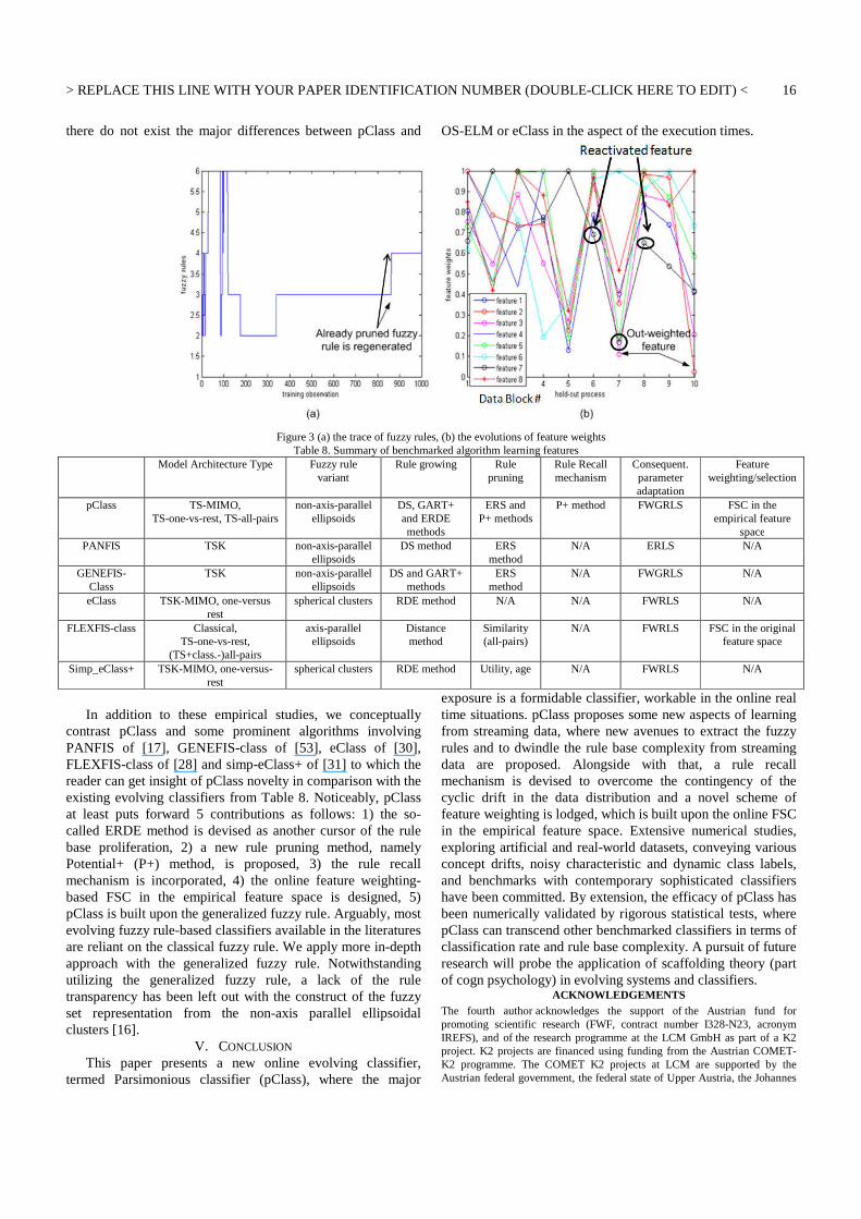
> REPLACE THIS LINE WITH YOUR PAPER IDENTIFICATION NUMBER (DOUBLE-CLICK HERE TO EDIT) <

16

there do not exist the major differences between pClass and OS-ELM or eClass in the aspect of the execution times.

Figure 3 (a) the trace of fuzzy rules, (b) the evolutions of feature weights

Table 8. Summary of benchmarked algorithm learning features Model Architecture Type Fuzzy rule

variant Rule growing Rule

pruning Rule Recall mechanism

Consequent. parameter adaptation

Feature weighting/selection

pClass TS-MIMO, TS-one-vs-rest, TS-all-pairs

non-axis-parallel ellipsoids

DS, GART+ and ERDE methods

ERS and P+ methods

P+ method FWGRLS FSC in the empirical feature

space PANFIS TSK non-axis-parallel

ellipsoids DS method ERS

method N/A ERLS N/A

GENEFIS-Class

TSK non-axis-parallel ellipsoids

DS and GART+ methods

ERS method

N/A FWGRLS N/A

eClass TSK-MIMO, one-versus rest

spherical clusters RDE method N/A N/A FWRLS N/A

FLEXFIS-class Classical, TS-one-vs-rest,

(TS+class.-)all-pairs

axis-parallel ellipsoids

Distance method

Similarity (all-pairs)

N/A FWRLS FSC in the original feature space

Simp_eClass+ TSK-MIMO, one-versus-rest

spherical clusters RDE method Utility, age N/A FWRLS N/A

In addition to these empirical studies, we conceptually

contrast pClass and some prominent algorithms involving PANFIS of [17], GENEFIS-class of [53], eClass of [30], FLEXFIS-class of [28] and simp-eClass+ of [31] to which the reader can get insight of pClass novelty in comparison with the existing evolving classifiers from Table 8. Noticeably, pClass at least puts forward 5 contributions as follows: 1) the so-called ERDE method is devised as another cursor of the rule base proliferation, 2) a new rule pruning method, namely Potential+ (P+) method, is proposed, 3) the rule recall mechanism is incorporated, 4) the online feature weighting-based FSC in the empirical feature space is designed, 5) pClass is built upon the generalized fuzzy rule. Arguably, most evolving fuzzy rule-based classifiers available in the literatures are reliant on the classical fuzzy rule. We apply more in-depth approach with the generalized fuzzy rule. Notwithstanding utilizing the generalized fuzzy rule, a lack of the rule transparency has been left out with the construct of the fuzzy set representation from the non-axis parallel ellipsoidal clusters [16].

V. CONCLUSION This paper presents a new online evolving classifier,

termed Parsimonious classifier (pClass), where the major

exposure is a formidable classifier, workable in the online real time situations. pClass proposes some new aspects of learning from streaming data, where new avenues to extract the fuzzy rules and to dwindle the rule base complexity from streaming data are proposed. Alongside with that, a rule recall mechanism is devised to overcome the contingency of the cyclic drift in the data distribution and a novel scheme of feature weighting is lodged, which is built upon the online FSC in the empirical feature space. Extensive numerical studies, exploring artificial and real-world datasets, conveying various concept drifts, noisy characteristic and dynamic class labels, and benchmarks with contemporary sophisticated classifiers have been committed. By extension, the efficacy of pClass has been numerically validated by rigorous statistical tests, where pClass can transcend other benchmarked classifiers in terms of classification rate and rule base complexity. A pursuit of future research will probe the application of scaffolding theory (part of cogn psychology) in evolving systems and classifiers.

ACKNOWLEDGEMENTS The fourth author acknowledges the support of the Austrian fund for promoting scientific research (FWF, contract number I328-N23, acronym IREFS), and of the research programme at the LCM GmbH as part of a K2 project. K2 projects are financed using funding from the Austrian COMET-K2 programme. The COMET K2 projects at LCM are supported by the Austrian federal government, the federal state of Upper Austria, the Johannes

> REPLACE THIS LINE WITH YOUR PAPER IDENTIFICATION NUMBER (DOUBLE-CLICK HERE TO EDIT) <

17

Kepler University and all of the scientific partners which form part of the K2-COMET Consortium. This publication reflects only the authors' views.

REFERENCES [1] V. N. Vapnik, The Statistical Learning Theory. New York: Springer-

Verlag, 1998 [2] S. Haykin, Neural Networks: A Comprehensive Foundation (2nd

Edition), Prentice Hall inc., Upper Saddle River, New Jersey, 1999 [3] G.-B. Huang,Q.-Y. Zhu and C.-K. Siew “Extreme Learning Machine:

Theory and Applications” Neurocomputing, vol.70 (1-3), pp.489-501, (2006)

[4] X. Wu, V. Kumar, J.R. Quinlan, J. Gosh, Q. Yang, H. Motoda, G.J. MacLachlan, A. Ng, B. Liu, P.S. Yu, Z.-H. Zhou, M. Steinbach, D.J. Hand and D. Steinberg, Top 10 algorithms in data mining, Knowledge and Information Systems, vol. 14 (1), pp. 1-37, (2006)

[5] E. Lughofer and P. Angelov, Handling Drifts and Shifts in On-line Data Streams with Evolving Fuzzy Systems, Applied Soft Computing, vol. 11(2), pp. 2057--2068, 2011

[6] H. Ishibuchi and T. Nakashima, Effect of rule weights in fuzzy rule-based classification systems, IEEE Transactions on Fuzzy Systems, vol. 9 (4), pp. 506--515, 2001

[7] N.-Y. Liang, G.-B. Huang, P. Saratchandran, and N. Sundararajan “ A Fast and Accurate On-line Sequential Learning Algorithm for Feedforward Networks”, IEEE Transactions on Neural Networks, vol.17(6), pp.1411-1423, (2006)

[8] A.Bouchachia, R.Mittermeir, “ Towards Incremental Fuzzy Classifiers”, Soft Computing, vol.11, pp.193-207, (2007)

[9] S.Pang, S.Ozawa, N.Kasabov, “Incremental Linear Discriminant Analysis for Classification of Data Streams”, IEEE Transactions on System, Man and Cybernetics-Part : Cybernetics, Vol.35(5),pp.905-914, (2005)

[10] C. Diehl and G. Cauwenberghs, “SVM incremental learning, adaptation and optimization,” in Proceedings of the International Joint Conference on Neural Networks Vol. 4, Boston, 2003, pp. 2685–2690, (2005)

[11] R.Zhang, G-B Huang, N.Sundarajanan, P.Saratchandran,” Improved GAP-RBF Network for Classification Problems”, Neurocomputing, Vol.70, pp.3011-3018, (2002)

[12] G.-B. Huang, P. Saratchandran, N. Sundararajan, An efficient sequential learning algorithm for growing and pruning RBF (GAP-RBF) networks, IEEE Transactions on Systems, Man and Cybernetic., part-B: Cybernetics, vol.34, pp. 2284–2292, (2004)

[13] G.-B. Huang, P. Saratchandran, and N. Sundararajan, A generalized growing and pruning RBF (GGAP-RBF) neural network for function approximation, IEEE Transactions on. Neural Networks.vol 16, pp. 57–67, (2005)

[14] A.Bouchachia, “ An Evolving Classification Cascade with Self-Learning”, Evolving System, Vol.1 (3), pp.143-160, (2010)

[15] P.Angelov and D. Filev, "An approach to online identification of Takagi-Sugeno fuzzy models," IEEE Transactions on Systems, Man, and Cybernetics, Part B: Cybernetics, vol. 34, pp. 484-498 (2004)

[16] M.Pratama, S.Anavatti, P.Angelov, E.Lughofer, PANFIS: A Novel Incremental Learning, IEEE Transactions on Neural Networks and Learning Systems, online and in press, 2013.

[17] M.Pratama, S.Anavatti, M.Garratt, E.Lughofer, “ Online Identification of Complex Multi-Input-Multi-Output System Based on GENERIC Evolving Neuro-Fuzzy Inference System”, in Proceedings of the Symposium Series on Computational Intelligence, Singapore, 2013.

[18] M.Pratama, M-J.Er, X.Li, R.J.Oentaryo, E. Lughofer, I.Arifin, “Data Driven Modelling Based on Dynamic Parsimonious Fuzzy Neural Network”, Neurocomputing, vol. 110, pp. 18-28, 2013

[19] M.Pratama, S.Anavatti, E.Lughofer, “GENFIS: Towards An Effective Localist Network”, IEEE Transactions on Fuzzy Systems, on line and in press, (2013)

[20] R.J.Oentaryo, M.J.Er, L.San, L-Y.Zhai, X.Li, “ Bayesian ART-Based Fuzzy Inference System: A New Approach to Prognosis of Machining Process”, IEEE Annual Conference of The Prognostic and Health Society, 2011.

[21] P. Angelov, Evolving Takagi-Sugeno Fuzzy Systems from Data Streams (eTS+), In Evolving Intelligent Systems: Methodology and Applications (Angelov P., D. Filev, N. Kasabov Eds.), John Willey and Sons, IEEE Press Series on Computational Intelligence, pp. 21-50, ISBN: 978-0-470-28719-4, April 2010.

[22] P.Angelov and D. Filev, "Simpl_eTS: A simplified method for learning evolving Takagi-Sugeno fuzzy models," in IEEE International Conference on Fuzzy Systems (FUZZ), pp. 1068-1073.(2005)

[23] H,Han, J.Qiao, “A Self-Organizing Fuzzy Neural Network Based on a Growing-and-Pruning Algorithm”, IEEE Transactions on Fuzzy System, vol.. 18(6), pp. 1129-1143, (2010).

[24] G. Leng, T.M. McGinnity, G. Prasad, Design for Self Organizing Fuzzy Neural Network Based on Genetic Algorithm, IEEE Transactions on Fuzzy Systems, vol. 14(6), pp. 755-766, (2006)

[25] E. Lughofer, Evolving Fuzzy Systems --- Methodologies, Advanced Concepts and Applications, Springer, Heidelberg, (2011)

[26] Zadeh, L. A. Soft computing and fuzzy logic. IEEE Software, 11,48–56.(1994)

[27] J. C. Bezdek, J. Keller, R. Krishnapuram, and N. R. Pal, Fuzzy Models and Algorithms for Pattern Recognition and Image Processing. Norwell, MA: Kluwer, (1999)

[28] P. Angelov, E. Lughofer, and X. Zhou, “Evolving fuzzy classifiers using different model architectures,” Fuzzy Sets and Systems, vol. 159(23), pp. 3160–3182, (2008)

[29] E.Lughofer,“On-line incremental feature weighting in evolving fuzzy classifiers,” Fuzzy Sets and Systems, vol. 163(1), pp. 1–23, (2011)

[30] P. Angelov and X. Zhou, “Evolving fuzzy-rule-based classifiers from data streams,” IEEE Transactions on Fuzzy Systems, vol. 16(6), pp. 1462–1475, (2008)

[31] R.D.Baruah, P.Angelov, J.Andreu, “ Simpl_eClass: Simplified Potential-Free Evolving Fuzzy Rule-Based Classifiers”, In: Proceedings of 2011 IEEE International Conference on Systems, Man and Cybernetics, SMC 2011, Anchorage, Alaska, USA, 7-9 Oct, 2011. IEEE, 2011. pp. 2249-2254

[32] A. Lemos, W. Caminhas and F. Gomide, Adaptive fault detection and diagnosis using an evolving fuzzy classifier, Information Sciences (special issue on Online Fuzzy Machine Learning and Data Mining), vol. 220, pp. 64--85, (2013)

[33] H-J.Rong, N.Sundarajan, G-B.Huang, G-S Zhao, “ Extended Sequential Adaptive Fuzzy Inference System for Classification Problems”, Evolving System, Vol.2 (2), pp.71-82, (2011)

[34] H.Xiong, M.N.S.Swamy, M.O.Ahmad,” Optimizing The Kernel in The Empirical Feature Space”, IEEE Transactions on Neural Networks, Vol.16(2), pp.460-474, (2005)

[35] M.Ramona, G.Riachard, B.David, “ Multiclass Feature Selection with Kernel Gram-Matrix-Based Criteria”, IEEE Transactions on Neural Networks and Learning Systems, Vol.23 (10), pp.1611-1622, (2012)

[36] H. Ishibuchi and T. Nakashima, Effect of rule weights in fuzzy rule-based classification systems, IEEE Transactions on Fuzzy Systems, vol. 9 (4), pp. 506--515, (2001)

[37] Y.Xu, K.W.Wong, C.S.Leung, “ Generalized Recursive Least Square to The Training of Neural Network”, IEEE Transactions on Neural Networks, Vol.17 (1), (2006)

[38] E.Lughofer, O.Buchtala, “ Reliable All-Pairs Evolving Fuzzy Classifiers”, IEEE Transactions on Fuzzy Systems, Vol.21 (4), pp. 625-641, (2013)

[39] E. Hüllermeier and K. Brinker, Learning Valued Preference Structures for Solving Classification Problems, Fuzzy Sets and Systems, vol. 159 (18), pp. 2337--2352, (2008)

[40] L.Wang, H-B.Ji, Y.Jin, “ Fuzzy Passive-Aggressive Classification: A Robust and Efficient Algorithm for Online Classification Problems”, Information Sciences, Vol.220,pp.46-63, (2013)

[41] P. Angelov, Evolving Takagi-Sugeno Fuzzy Systems from Data Streams (eTS+), In Evolving Intelligent Systems: Methodology and Applications (Angelov P., D. Filev, N. Kasabov Eds.), John Willey and Sons, IEEE Press Series on Computational Intelligence, pp. 21-50, ISBN: 978-0-470-28719-4, April (2010)

[42] E.Lughofer, “A Dynamic Split-and-Merge Approach for Evolving Cluster Models”, Evolving Systems, Vol.3 (3), pp.135-151, (2012)

[43] B. Vigdor and B. Lerner, “The Bayesian ARTMAP,” IEEE Transactions on Neural Networks, vol. 18(6), pp. 1628–1644, (2007)

[44] J. J. Rubio, SOFMLS: Online Self-Organizing Fuzzy Modified Least Square Network, IEEE Transactions on Fuzzy Systems, Vol. 17, No. 6, pp. 1296-1309, 2009

[45] P. Angelov, A. Kordon, Adaptive Inferential Sensors Based on Evolving Fuzzy Models, IEEE Transactions on Systems, Man, and Cybernetics, Part B: Cybernetics, Vol. 40, No. 2, pp. 529-539, (2010)

> REPLACE THIS LINE WITH YOUR PAPER IDENTIFICATION NUMBER (DOUBLE-CLICK HERE TO EDIT) <

18

[46] J-C.de Barros, A.L.Dexter, “ On-line Identification of Computationally Undemanding Evolving Fuzzy Models”, Fuzzy Sets and Systems, Vol.158, pp.1997-2012, (2007)

[47]Y-C.Chen, N.R.Pal, I-F.Chung, “ An Integrated Mechanism for Feature Selection and Fuzzy Rule Extraction to Classifications”, IEEE Transactions on Fuzzy Systems, Vol.20 (2), pp.683-698, (2012)

[48]N.R.Pal, S.Saha, “ Simultaneous Structure Identification and Rule Generations for Takagi-Sugeno Models”, IEEE Transactions on Systems, Man and Cybernetics-part B: Cybernetics, Vol.38(6), pp.1626-1638, (2008)

[49] J. J. Rubio, J. H. Pérez-Cruz, Evolving intelligent system for the modelling of nonlinear systems with dead-zone input, Applied Soft Computing, online and in press, (2013)

[50] J. J. Rubio, D. M. Vazquez, D. Mujica-Vargas, Acquisition system and approximation of brain signals, IET Science, Measurement and Technology, 2013.

[51] A. Asuncion and D. J. Newman. (2007). UCI Machine Learning Repository [Online]. School of Information and Computer Science, University of California, Irvine. Available: http://www.ics.uci.edu/mlearn/MLRepository.html

[52] M.Stone, “Cross-Validatory Choice and Assessment of Statistical Predictions”, Journal of Royal Statistic Society, vol.36, pp. 111-147, (1974)

[53] M.Pratama, S.Anavatti, E.Lughofer, “ Evolving Fuzzy Rule-Based Classifier Based on GENEFIS”, Proceedings of the IEEE Conference on Fuzzy Systems, Hyderabad, India, 2013

[54] S.Suresh, K.Dong, H.J.Kim, “ A Sequential Learning Algorithm for Self-Adaptive Resource Allocation Network Classifier”, Neurocomputing, Vol.73, pp.3012-3019, (2010)

[55] W.N.Street, Y.Kim, “A streaming ensemble algorithm SEA for large- scale classification”, in the proceeding of 7th ACM SIGKDD, pp 377-382, (2001)

[56] E. Lughofer, On-line Evolving Image Classifiers and Their Application to Surface Inspection, Image and Vision Computing, Vol.28 (7), pp.1065–1079,(2010)

[57] A. Bifet, G. Holmes, R. Kirkby, and B. Pfahringer, “MOA: Massive online analysis,” Journal of Machine Learning Research, vol. 11, pp.1601–1604, (2010)

[58]L.LMinku, X.Yao, “ DDD: A New Ensemble Approach for Dealing with Drifts”, IEEE Transactions on Knowledge and Data Engineering, Vol.24(4), 2012

[59]L.L.Minku, A.P.White, X.Yao, “ The Impact of Diversity on Online Ensemble Learning in The Presence Concept of Drift”, IEEE Transactions on knowledge and Data Engineering, Vol.22(5),2010

[60] E-Y.Cheu, C.Quek, S-K.Ny, ARPOP: An Appretitive Reward-Based Pseudo-Outer-Product Neural Fuzzy Inference System Inspired from The Operant Conditioning of Feeding Behaviour in Aplysia, IEEE Transactions on Neural Networks and Learning Systems, Vol.23(2), (2012)

[61] J.Demsar, “ Statistical Comparisons of Classifiers over Multiple Datasets”, Journal of Machine Learning Research, Vol.7, pp.1-30, 2006

Mahardhika Pratama, was born in Surabaya, Indonesia. He received B.Eng degree (First Class Honor) in Electrical Engineering from the Sepuluh Nopember Institute of Technology, Indonesia, in 2010. At the same time, he was awarded the best and most favorite final project by the same institution. Mr. Pratama holds his Master of Science (M.Sc) degree in Computer Control and Automation (CCA) from Nanyang Technological University,

Singapore, in 2011 and achieved prestigious engineering achievement award given by Institute of Engineer, Singapore. He currently pursues a PhD program in University of New South Wales, Australia, where he was awarded the high impact publication award in 2013. Mr.Pratama is a member of IEEE, IEEE Computational Intelligent Society (CIS) and IEEE System, Man and Cybernetic Society (SMCS), and Indonesian Soft Computing Society (ISC-INA) and is an active reviewer in some top tier journals such as: IEEE Transactions on System, Man and Cybernetics part-B: Cybernetics,

Neurocomputing and Applied Soft Computing. His research interests involve machine learning, computational intelligent, evolutionary computation, fuzzy logic, neural network and evolving adaptive systems.

Sreenatha Anavatti received his Ph.D degree in aerospace engineering from the Indian Institute of Science in 1990, his Bachelor of Engineering degree in mechanical engineering from the Mysore University, India in 1984. He is currently a Senior Lecturer at the School of Aerospace, Civil and Mechanical Engineering (ACME), University of New South Wales at Australian Defence Force Academy (UNSW@ADFA), Australia.

His current research interests include control systems, flight dynamics, robotics, aeroelasticity, artificial neural networks, fuzzy systems and unmanned systems.

Professor Er Meng Joo is currently a Full Professor in Electrical and Electronic Engineering, Nanyang Technological University, Singapore. He has authored 5 books, 16 book chapters and more than 400 refereed journal and conference papers in his research areas of interest. His areas of research interests are Intelligent control theory and applications, computational intelligence, robotics and automation, sensor networks, biomedical engineering

and cognitive science. Currently, Professor Er serves as the Editor-in-Chief of the Transactions on Machine Learning and Artificial Intelligence and International Journal of Electrical and Electronic Engineering and Telecommunications, an Area Editor of International Journal of Intelligent Systems Science, an Associate Editor of eleven refereed international journals including the IEEE Transaction on Fuzzy Systems and an editorial board member of the EE Times.

Edwin David Lughofer received his PhD. degree from the Department of Knowledge-Based Mathematical Systems, University Linz. He is now employed as key researcher at the department’s branch Fuzzy Logic Laboratorium in the Softwarepark Hagenberg. He participated in several international research (EU) projects and has published more than 100 journal and conference papers in the fields of evolving fuzzy systems, machine learning and vision, clustering, fault

detection, including a monograph on ‘Evolving Fuzzy Systems’ (Springer, Heidelberg) and an edited book on ‘Learning in Non-stationary Environments’ (Springer, New York). He acts as a reviewer in peer-reviewed international journals and as (co-)organizer of special sessions and issues at international conferences and journals. In 2014, he served as Main Chair of the international IEEE conference on Evolving and Adaptive Intelligent Systems. He served as programme committee member in several international conferences and is a member of the editorial board and associate editor of the international Springer journal ‘Evolving Systems’ and the international Elsevier Journal ‘Information Fusion’. In 2006 he received the best paper award at the International Symposium on Evolving Fuzzy Systems, and in 2013 the best paper award at the IFAC conference in Manufacturing Modeling, Management and Control Conference.