DOCTORAL THESIS

Mgr. Michal Brabec

Procedural code integration instreaming environments

Department of Software Engineering

Supervisor of the doctoral thesis: David Bednarek, Ph.D.

Study programme: 4I2, Softwarove systemy

Study branch: Compilers

Prague 2017

I declare that I carried out this doctoral thesis independently, and only with thecited sources, literature and other professional sources.

I understand that my work relates to the rights and obligations under the ActNo. 121/2000 Sb., the Copyright Act, as amended, in particular the fact that theCharles University has the right to conclude a license agreement on the use ofthis work as a school work pursuant to Section 60 subsection 1 of the CopyrightAct.

In Prague date 12.12.2017 Mgr. Michal Brabec

Title: Procedural code integration in streaming environments

Author: Mgr. Michal Brabec

Department: Department of Software Engineering

Supervisor: David Bednarek, Ph.D.

Abstract: Streaming environments and similar parallel platforms are widely usedin image, signal, or general data processing as means of achieving high perfor-mance. Unfortunately, they are often associated with domain specific program-ming languages, and thus hardly accessible for non-experts. In this work, wepresent a framework for transformation of a procedural code to a streaming ap-plication. We selected a restricted version of the C# language as the interface forour system, because it is widely taught and many programmers are familiar withit. This approach will allow creating streaming applications or their parts usinga widely known imperative language instead of the intricate languages specific tostreaming.

The transformation process is based on the Hybrid Flow Graph – a novel inter-mediate code which employs the streaming paradigm and can be further convert-ed into streaming applications. The intermediate code shares the features andlimitations of the streaming environments, while representing the applicationswithout platform specific technical details, which allows us to use well knowngraph algorithms to work with the code efficiently.

In this work, we present the entire transformation process from the C# codethe complete streaming application. This includes the management of the con-trol flow, data flow, processing of arrays, method integration and optimizationsnecessary to produce efficient applications. Control flow represents the main dif-ference between procedural code, driven by control flow constructs, and streamingenvironments, driven by data. We transform the code directly into the HybridFlow Graph and then we optimize the graph to introduce a structure better suitedfor the streaming environments. Finally we transform the graph into a streamingapplication.

We use procedurally generated code to verify the framework’s correctness, wherewe test methods containing all combinations of loops, branches and serial codenested in each other. We also evaluate the performance of the produced applica-tions and since the use of a streaming platform automatically enables parallelismand vectorization, we were able to demonstrate that the streaming applicationsgenerated by our method may outperform their original C# implementation.

Keywords: code transformation; intermediate code; parallel programming; vec-torization; streaming systems;

I would like to give many thanks to all the people who helped me with this workand all the research leading up to it. First of all, I would like to thank my advisorDavid Bednarek, Ph.D. who helped me tremendously with my research, and hisadvice was indispensable for all my publications. I would also like to thank allmy other colleagues from the university, who provided technical expertise andsupport.

Next, I would like to thank my family for understanding and support. Specialthanks to my wife Klara, who believed in me all the way through.

Finally, I would like to thank my coworkers for creative environment, supportand important feedback.

Contents

1 Introduction 51.1 Motivation . . . . . . . . . . . . . . . . . . . . . . . . . . . . . . . 71.2 Objectives . . . . . . . . . . . . . . . . . . . . . . . . . . . . . . . 81.3 Contributions . . . . . . . . . . . . . . . . . . . . . . . . . . . . . 81.4 Text Structure . . . . . . . . . . . . . . . . . . . . . . . . . . . . . 9

2 Streaming Environments 112.1 Related Work – Streaming Environments . . . . . . . . . . . . . . 122.2 Configuration and Programming . . . . . . . . . . . . . . . . . . . 142.3 Available Parallelism . . . . . . . . . . . . . . . . . . . . . . . . . 162.4 Performance Concerns . . . . . . . . . . . . . . . . . . . . . . . . 17

3 Common Techniques 193.1 Graph Rewriting Systems . . . . . . . . . . . . . . . . . . . . . . 19

3.1.1 Associative Graph Rewriting Systems . . . . . . . . . . . . 203.1.2 Graph Rewriting System Use Cases . . . . . . . . . . . . . 21

3.2 Kahn Process Networks . . . . . . . . . . . . . . . . . . . . . . . . 213.3 CIL Basics . . . . . . . . . . . . . . . . . . . . . . . . . . . . . . . 22

3.3.1 Common Language Runtime . . . . . . . . . . . . . . . . . 223.3.2 Common Intermediate Language . . . . . . . . . . . . . . 23

3.4 SIMD Instructions . . . . . . . . . . . . . . . . . . . . . . . . . . 253.4.1 Vectorization . . . . . . . . . . . . . . . . . . . . . . . . . 253.4.2 SIMD Instructions Types . . . . . . . . . . . . . . . . . . . 253.4.3 Memory Organization . . . . . . . . . . . . . . . . . . . . 273.4.4 SIMD in C++ . . . . . . . . . . . . . . . . . . . . . . . . . 27

4 Hybrid Flow Graph 294.1 Related Work – Hybrid Flow Graph . . . . . . . . . . . . . . . . . 314.2 Basic Operation Semantics . . . . . . . . . . . . . . . . . . . . . . 324.3 Representation of Control Flow . . . . . . . . . . . . . . . . . . . 334.4 Hybrid Flow Graph Execution . . . . . . . . . . . . . . . . . . . . 354.5 Layered Hybrid Flow Graph . . . . . . . . . . . . . . . . . . . . . 36

5 Compiler for Streaming Environments 395.1 Related Work – Intermediate Code and Parallelism . . . . . . . . 395.2 Compiler Architecture . . . . . . . . . . . . . . . . . . . . . . . . 405.3 Input Language Restrictions . . . . . . . . . . . . . . . . . . . . . 42

6 Compiler Front-end 456.1 Front-end Overview . . . . . . . . . . . . . . . . . . . . . . . . . . 45

6.1.1 Transformation Example . . . . . . . . . . . . . . . . . . . 466.2 Related Work – Compiler Front-end . . . . . . . . . . . . . . . . . 466.3 Method Selection . . . . . . . . . . . . . . . . . . . . . . . . . . . 486.4 Method Integration . . . . . . . . . . . . . . . . . . . . . . . . . . 49

6.4.1 Integration overview . . . . . . . . . . . . . . . . . . . . . 506.4.2 Variable Renaming . . . . . . . . . . . . . . . . . . . . . . 50

1

6.4.3 Parameter Patch . . . . . . . . . . . . . . . . . . . . . . . 506.4.4 Jump Extension . . . . . . . . . . . . . . . . . . . . . . . . 516.4.5 Code Integration . . . . . . . . . . . . . . . . . . . . . . . 516.4.6 Stack Limit . . . . . . . . . . . . . . . . . . . . . . . . . . 51

6.5 Code Preprocessing . . . . . . . . . . . . . . . . . . . . . . . . . . 526.6 Data Flow Analysis . . . . . . . . . . . . . . . . . . . . . . . . . . 53

6.6.1 CIL Sequential Graph . . . . . . . . . . . . . . . . . . . . 546.6.2 Symbolic Semantics of the CIL Sequential Graph . . . . . 576.6.3 Execution of the Symbolic CIL Sequential Graph . . . . . 586.6.4 Construction of the CIL Sequential Graph . . . . . . . . . 596.6.5 Instruction Classifier . . . . . . . . . . . . . . . . . . . . . 60

6.7 Control Flow Analysis . . . . . . . . . . . . . . . . . . . . . . . . 626.7.1 Branch Infrastructure . . . . . . . . . . . . . . . . . . . . . 636.7.2 Loop Infrastructure . . . . . . . . . . . . . . . . . . . . . . 646.7.3 Control-Flow Analysis Overview . . . . . . . . . . . . . . . 646.7.4 Hybrid Flow Graph Construction . . . . . . . . . . . . . . 656.7.5 Broadcast Introduction . . . . . . . . . . . . . . . . . . . . 676.7.6 Source Code and HFG Equivalence . . . . . . . . . . . . . 69

6.8 Data types . . . . . . . . . . . . . . . . . . . . . . . . . . . . . . . 706.9 Array Support . . . . . . . . . . . . . . . . . . . . . . . . . . . . . 706.10 Aliasing . . . . . . . . . . . . . . . . . . . . . . . . . . . . . . . . 71

7 Optimization 737.1 Related Work – Transformations Improving Parallelism . . . . . . 747.2 Component Extraction . . . . . . . . . . . . . . . . . . . . . . . . 757.3 Dead and Empty Nodes Elimination . . . . . . . . . . . . . . . . 767.4 Range Extraction . . . . . . . . . . . . . . . . . . . . . . . . . . . 777.5 Array Extraction . . . . . . . . . . . . . . . . . . . . . . . . . . . 787.6 Token Extraction . . . . . . . . . . . . . . . . . . . . . . . . . . . 807.7 Vectorization . . . . . . . . . . . . . . . . . . . . . . . . . . . . . 817.8 Array Extraction and Vectorization Chaining . . . . . . . . . . . . 81

8 Compiler Back-end 838.1 Related Work – Compiler Back-end . . . . . . . . . . . . . . . . . 838.2 Supported Environments . . . . . . . . . . . . . . . . . . . . . . . 838.3 Bobox Transformation . . . . . . . . . . . . . . . . . . . . . . . . 848.4 Transformation Overview . . . . . . . . . . . . . . . . . . . . . . . 848.5 Execution Plan Construction . . . . . . . . . . . . . . . . . . . . . 858.6 Component Extraction . . . . . . . . . . . . . . . . . . . . . . . . 86

9 Additional Environments 899.1 .NET Asynchronous Method . . . . . . . . . . . . . . . . . . . . . 89

9.1.1 Transformation Overview . . . . . . . . . . . . . . . . . . 899.1.2 Graph Without Control-Flow . . . . . . . . . . . . . . . . 909.1.3 Branch Transformation . . . . . . . . . . . . . . . . . . . . 909.1.4 Loop Transformation . . . . . . . . . . . . . . . . . . . . . 91

9.2 Managed Bobox Integration . . . . . . . . . . . . . . . . . . . . . 929.2.1 Graph Execution . . . . . . . . . . . . . . . . . . . . . . . 939.2.2 Graph Integration . . . . . . . . . . . . . . . . . . . . . . . 93

2

10 Case Study: Matrix-based Dynamic Programming 9710.1 Problem Details . . . . . . . . . . . . . . . . . . . . . . . . . . . . 9810.2 Related Work – Matrix-based Dynamic Programming Parallelization 9910.3 Levenshtein Distance Blocked Algorithm . . . . . . . . . . . . . . 99

10.3.1 Parallelogram Blocks . . . . . . . . . . . . . . . . . . . . . 10010.3.2 Blocked Algorithm . . . . . . . . . . . . . . . . . . . . . . 101

10.4 Matrix-based Dynamic Programming in Streaming Environments 10110.4.1 Blocked Algorithm Implementation in C# . . . . . . . . . 10110.4.2 Blocked Algorithm in ParallaX Compiler . . . . . . . . . . 104

11 Experiments 10711.1 Correctness Experiments . . . . . . . . . . . . . . . . . . . . . . . 10711.2 Levenshtein Distance Experiments . . . . . . . . . . . . . . . . . . 10911.3 Streaming Experiments . . . . . . . . . . . . . . . . . . . . . . . . 113

11.3.1 Convolution Experiment . . . . . . . . . . . . . . . . . . . 11411.3.2 Cryptography Experiment . . . . . . . . . . . . . . . . . . 11411.3.3 Baseline Experiments . . . . . . . . . . . . . . . . . . . . . 11611.3.4 Single Filter . . . . . . . . . . . . . . . . . . . . . . . . . . 11711.3.5 Serial Filter . . . . . . . . . . . . . . . . . . . . . . . . . . 11811.3.6 Multiple Filter . . . . . . . . . . . . . . . . . . . . . . . . 11911.3.7 Experiment Conclusions . . . . . . . . . . . . . . . . . . . 120

12 Conclusions 12112.1 Future Work . . . . . . . . . . . . . . . . . . . . . . . . . . . . . . 122

Appendix A: Compiler Infrastructure 12312.2 Compiler Work Flow . . . . . . . . . . . . . . . . . . . . . . . . . 12312.3 Application structure . . . . . . . . . . . . . . . . . . . . . . . . . 12412.4 Compiler Configuration . . . . . . . . . . . . . . . . . . . . . . . . 125

12.4.1 Configuration File . . . . . . . . . . . . . . . . . . . . . . 12512.4.2 Transformation File . . . . . . . . . . . . . . . . . . . . . . 126

Appendix A: Compiler Library 129

Bibliography 129

Attachments: Digital Content 139

Index 141

Bibliography of the Author 142

3

4

1. Introduction

Streaming environments form an important niche of parallel computing, original-ly designed for efficient implementation of image or digital signal processing. Asthese application domains interacted with other areas, particularly with databas-es, the idea of streaming environments developed from simple fixed-rate pipelinestowards systems allowing arbitrary networks of operators with variable data rates.In addition, many parallel software systems resemble streaming environment, al-though they are not categorized as streaming.

Gradually, streaming environments became almost universal parallel comput-ing platforms; however, no widely accepted standard emerged yet. Thus, eachstreaming platform often consists of a specialized language, its compiler, andone or more run-time environments, targeted at special hardware (like FPGA),GPUs, and/or general CPUs. An application is either constructed completely ina stream-specific language or it incorporates parts (kernels) written in a generallanguage like C or VHDL.

With respect to performance, the specialized streaming languages may haveimportant advantages including enforcing a particular (i.e. streaming) program-ming style and the absence of optimization disablers (like unrestricted memoryaccess and aliasing) known from general-purpose procedural languages. On theother hand, programming streaming systems is a kind of rare expert knowledge.Moreover, the interaction between streaming and traditional code is often diffi-cult; therefore, it might be advantageous to introduce a compiler able to createstreaming applications from a procedural code.

Thus, allowing the use of a well-known general programming language for thedesign of streaming applications would allow the participation of non-experts whodo not posses the knowledge of the required streaming language or the intricatedetails of the system interfaces. It would also make existing code available forthe use in streaming systems.

In our research, we investigate whether modern general programming lan-guages like C# may be used in streaming systems and, in particular, whether acompiler may convert non-parallel C# code into a network of operators whichcould be executed by a streaming runtime environment. Our research is target-ed at streaming platforms implemented on general purpose CPUs and allowingvariable data rates using a dynamic scheduler.

We wanted a language widely known among current programmers and re-searchers, which ruled out older languages like Fortran. We wanted a languagewith a comprehensive intermediate code so we could avoid the necessity to imple-ment parser of the input language and this narrowed the choice to either Java orC#. We selected C#, because its intermediate language and entire environmentis standardized and C# supports structures – object types with value semantics.Another advantage is the Cecil library which provides great tools for work withthe C# intermediate code (CIL).

In shared-memory implementations of streaming systems, the overhead ofdata communication may be as low as writing and reading memory or cache.Thus, parallelism may be improved by decomposing an application into a largenumber of very small components, each comprising of only a handful or few

5

C#

source code

CIL code

HFGC#

compiler

Graph

construction

Component

extraction

Code

generation

Global

HFG

Layered

HFG

Runtime

environment

Plan

generation

front-end optimization back-end

Figure 1.1: Compilation and code generation

dozens of arithmetic operations. This arrangement also naturally supports theuse of vector operations.

Our target architecture is illustrated in Figure 1.1. In this case, a sourcecode in C# is compiled (by a standard C# compiler) into the CIL intermediatecode and then converted into the Hybrid Flow Graph(HFG) intermediate code[3]. While the CIL code is a classical intermediate code based on sequences ofinstructions, the HFG code assumes the form of a network of communicatingoperators; thus, it corresponds to the architecture of the run-time system, albeitin much finer granularity.

At this stage, the operators are equivalents of individual CIL instructions;therefore they are typically too small to become an efficient streaming operator.Consequently, in the next stage, the optimization technique called componentextraction rearranges the original operators into small groups, producing a layeredHFG containing a subgraph for each such group and a global HFG describingthe interaction between the groups. For each component HFG, executable codecorresponding to a streaming operator is generated. The global HFG is convertedto a plan which defines the run-time connections (i.e. streams) between theoperators.

In this work, we present theoretical basis of the Hybrid Flow Graph formal-ism, followed by the description of the graph extraction phase that converts asequential intermediate code into the HFG. Next, we present the graph optimiza-tion – component extraction and its transformation into an application for theBobox streaming system. Since the HFG follows the data-flow paradigm of thestreaming systems, branches and loops must be converted from their sequentialform into flows of control data.

Note that function calls have to be eliminated from the converted C# pro-gram by means of procedure integration. Of course, procedure integration is notpossible in the presence of non-tail recursion and it may lead to unacceptable codeexpansion in some other cases; however, the same limitations typically apply alsoin streaming languages. In this work, we use a restricted version of the C# lan-guage, where we limit the use of referential data types (classes), assuming thatvalue types (including structures) and arrays are predominantly used in typicalstreaming applications. The restrictions are described and explained in detail inSection 5.3. Consequently, while our approach is obviously not applicable as a

6

method of converting arbitrary C# programs for execution by streaming systems,it is applicable as a new interface for the streaming systems.

In order to implement a compiler capable of producing the HFG code, we hadto implement multiple algorithms similar to those used in standard compilers, butmodified for the HFG intermediate language. In most cases it was necessary toslightly modify the algorithms so that they reflect the HFG structure. We pointout the algorithms in the sections focusing on related work, where we identify theoriginal algorithm and the changes necessary for it to work in our environment.

To estimate the performance of the applications produced by our compiler,we measured the performance of several algorithms, including the Levenshteindistance, in their original C# implementation as well as when converted intostreaming applications. Our measurements show that even the current proto-type implementation of our compiler is able to generate streaming code, whichis significantly faster than the original C# code. Additional optimizations mightfurther improve the performance of the produced applications.

1.1 Motivation

Many streaming environments are well suited for execution of database-like queries.However; creating applications by mixing declarative languages, like SQL, andprocedural components, like user-defined functions, is not easy in such environ-ments. The following example shows where our proposed system could improvethe situation:

select ∗ from T1 , T2 where T1 . r eg i on = T2 . r eg i on andDISTANCE( T1 . name , T2 . name) < 10

Listing 1.1: Sql query with a user-defined function

When implemented in a traditional database system, the query in Figure 1.1contains a custom (user-defined) function DISTANCE, usually programmed ina platform-specific procedural language, like PL/SQL in Oracle or PL/pgSQL inPostgreSQL. In the database systems, the SQL part of the query is transformedinto a highly optimized plan, where the T1 and T2 are initially joined based ontheir values and then the system applies the DISTANCE function.

The SQL plan is usually executed in a specialized environment provided bythe database engine, which contains optimized operators for all the standard SQLconstructs. However; the execution of the custom functions requires a differentenvironment, because they are implemented in a language with vastly differ-ent properties, which brings significant communication overhead. The matter isfurther complicated when the system tries to parallelize the custom functions,because they behave differently from the SQL operators and both can competefor resource.

One solution would be to transform the custom DISTANCE function intoan execution plan similar to that produced from SQL, connect both the planstogether and execute them in the same environment. This solution would not beideal, because both parts may have significantly different granularity. Therefore;parallelism will not be optimal due to different complexity and performance ofcomponents, but this approach eliminates communication overhead.

7

More advanced solution must incorporate decomposition of both the customfunctions and the SQL operators and then it has to provide a mechanism to groupsmaller components into bigger blocks. This way the decomposed operators andfunctions can be grouped according to the structure of the entire query, thusreducing the communication overhead and providing more efficient parallelism.This approach can improve the overall structure of the query, because it bypassesthe strict separation of custom functions and SQL operators and processes themall together.

The following two cases illustrate further benefits of the proposed solution:

1. The custom function can call other SQL commands. In this case, the ad-vanced solution might be able to merge both the SQL plans and the customfunction into a single query and optimize all its components together.

2. The custom function can be used to generate data. This might severelychange the behavior of the query, because the custom functions are treateddifferently. However; the proposed approach decomposes custom functionsand SQL operators and treats them the same, thus eliminating this problem.

It is important to note that in most cases, the custom functions are relativelysmall, without advanced constructs, like objects or exceptions. This allows us torestrict the input language while still providing sufficient tools for design of thesefunctions.

This work provides the basis for the advanced solution presented in this sec-tion. The ParallaX compiler produced as the main part of this work is ableto transform custom functions written in restricted C# to an intermediate lan-guage similar to the execution plans. Further work will be necessary to efficientlymerge and optimize the produced plans, but the difficult transformation from theprocedural code to the execution plan is solved in this work.

1.2 Objectives

Our main objective is to design an intermediate representation with propertiessimilar to the streaming environments, which would allow us to work with theapplications efficiently but without platform-specific limitations. This representa-tion would also allow us to transform the applications for multiple environmentsusing the same input language. To achieve this objective, we designed the HybridFlow Graph that is the main representation of the code in the compiler.

Our second objective is to facilitate the design of streaming applications toprogrammers without the domain specific knowledge of the streaming environ-ment or its associated languages. To achieve this objective, we designed a com-piler that transforms C# code, compiled to CIL, into applications for the Boboxstreaming system [2].

1.3 Contributions

• We have designed the Hybrid Flow Graph, which can be used to representapplications in a way that they can be executed in streaming environments

8

or on other similar platforms. The Hybrid Flow Graph could be used asa common representation of applications for multiple different streamingenvironments.

• We have designed the compiler front-end capable of transforming a C#code, compiled to CIL, into the Hybrid Flow Graph. The compiler is able totransform code between two different programming paradigms and producea representation suitable for streaming environments.

• We have designed a series of optimizations for the Hybrid Flow Graph, thatimprove its structure and behavior during execution.

• We have designed a compiler that transforms the Hybrid Flow Graph intoan application for the Bobox system. The HFG structure is transformedinto the domain-specific language Bobolang, while the separate kernels aretransformed into C++. The entire application is then compiled with theBobox runtime.

• We have modified algorithms and analyses, used in traditional compilers, forthe HFG intermediate language. The algorithms rely on the same theoret-ical basis, but reflect the structural specifics of a graph-based intermediatelanguage.

1.4 Text Structure

The rest of this work is organized as follows: After reviewing the general conceptsof the streaming environments in Chapter 2, we present the well-known techniquesand algorithms that form the basis of our work in Chapter 3. Next we define thestructure of the Hybrid Flow Graphs in Section 4, especially their componentsrelated to control flow handling.

The next chapters define parts of the compiler for streaming environment thatis the main contribution of this work. Chapter 5 sums the compiler’s generalconcepts and structure, Chapter 6 explains the transformation of the C# sourceto the intermediate language – the Hybrid Flow Graph, Chapter 7 defines theHFG optimizations and Chapter 8 focuses on the HFG transformation into theapplication for the Bobox streaming system.

After all the compiler details are explained, we present alternative targetenvironments supported by the compiler in Chapter 9. Chapter 10 presents ourmain case studies used to evaluate the performance of the applications producedby the compiler – the Levenshtein edit distance. Finally, section 11 illustratesthe performance reachable using the complete compilation chain.

9

10

2. Streaming Environments

Stream processing is a programming paradigm that simplifies parallelization ofsome applications by restricting their structure1. Limiting the application archi-tecture leads to better defined and more predictable behavior, which significantlyenhances available parallelism and can help with scheduling, distribution andload balancing. This also means that the application can automatically use mul-tiple CPUs and even heterogeneous processing units, such as graphical processors(GPUs) or field-programmable gate arrays (FPGAs), without explicitly managingmemory or synchronization.

Streaming processing paradigm defines the application general architecture.An application designed according to this paradigm is constructed from the fol-lowing components:

• Stream – a sequence of data.

• Kernel2 – a series of operations (a function) applied to each element of itsinput streams.

• Plan3 – an oriented graph, with nodes representing kernels and streamspassed along edges.

The most important aspect of the streaming processing architecture is thefact that the kernels are able to communicate only by passing data to the streamsconnecting them. Kernels cannot communicate through the memory, network orexternal storage. This principle is crucial to exposing the available parallelism.It is possible to allow some kernels to read or write data to external storage toprovide data for the application, but the locations should be independent, so thekernels do not influence one another.

Kernels can be either stateless or stateful depending on their semantics. Thestateless kernels do not store any state information and their output always de-pends solely on the actual inputs. Stateful kernels maintain internal state, whichcan influence their output.

Figure 2.1 shows a plan of a simple join that merges two sets of values readfrom a data source (database) by the kernels source1 and source2. The joincondition is implemented in the merge kernel. The plan declares kernels andtheir connections via streams, but it does not define the kernel implementation.Kernels are implemented separately as functions or objects, usually in a standardprocedural language, and together with the plan they comprise the application.

The start kernel in Figure 2.1 initiates the application execution, since it is theonly kernel without input. We use the start kernel to simplify the plan structure.The source kernels read the input from a data source (database or file), whilethe print kernel prints the result to the output (console).

1This chapter does not provide the analysis of all the systems that can be possibly cate-gorized as streaming environments. Instead, we focus only on the systems best suited for theimplementation of data-intensive application, like database queries.

2Alternatively called Operator or Box3Alternatively called Execution plan

11

broadcast

source2

merge

source1

start print

Figure 2.1: Simple join programmed for the Bobox streaming environment

A streaming environment is a system which is able to execute applicationsdesigned according to the streaming processing paradigm, also called streamingapplications . The environment defines supported languages for programming theseparate parts of the application. This usually means that the kernels are createdin some general programming language, while the plan is defined in some specialdeclarative language or constructed during runtime by explicit system calls.

Our selected target platform is the Bobox [2] streaming environment. It sup-ports kernels implemented as C++ classes and for the execution plan, Bobox usesa special declarative language called Bobolang [3].

The rest of this chapter will discuss important aspects of streaming environ-ments, with main focus on the Bobox system. We will explain how compatibleapplications are designed in Section 2.2. In Section 2.3, we will examine howthese systems expose and exploit available parallelism and in Section 2.4, we willfocus on factors that influence performance.

2.1 Related Work – Streaming Environments

This section presents other research related to the general concepts of this work,while the works related to the specific parts of our research are presented in latersections alongside the appropriate technique or algorithm. This approach meansthat the related works are discussed when relevant instead of being collected atthe beginning without connection to the actual algorithm or concept.

The definition of a streaming environment or system is not strict, the labelhas been applied to a broad range of systems. The lower tier is occupied withsystems designed for tight integration with hardware, often accompanied withcircuit synthesis or specialized hardware.

The Brook system adds simple parallelization constructs to the C language,allowing the programmers to use the GPU as a streaming co-processor [4]. TheBrook system provides extensions for the C language and a special runtime library.The applications are designed in the extended C, transformed into a code for thetarget environment (originally designed for DirectX and OpenGL) and compiledalong with the runtime library.

Esterel is a language for programming synchronous parallel reactive systems[5]. A system designed in the Esterel language consists of multiple components(modules), which communicate through signals broadcast through the entire sys-tem. Each component defines the signals it recognizes and actions it can perform.The components can react to the signals by initiating or terminating actions orproducing other signals. The language is the main programming environment forthe experimental Kiel Esterel Processor [6].

The StreaMIT language was designed as a tool for efficient development ofstreaming applications [7]. The language adds streaming constructs to a restricted

12

version of the Java language and the programmers use the constructs to definethe structure of the streaming applications (their plan, kernels and streams).The StreaMIT code is then compiled by a specialized compiler to a code for thetarget environment. The compiler is designed as an extension of the Kopi JavaCompiler.

All these streaming systems rely on their own platform-specific languages,which contain special constructs necessary to define the structure of the stream-ing applications. This approach requires that the programmers construct theapplication structure by hand, which means that they have to know the proper-ties of the constructs and target platform.

The field-programmable gate array (FPGA) can be considered a special caseof low-level streaming hardware, where the separate programmable gates repre-sent kernels. The FPGAs are traditionally programmed in a low-level hardwaredescription language (HDL), but there are purely streaming technologies devel-oped over it, like the Folding Streams algorithm [8], which generates the HDLcode from a declarative implementation.

The upper tier of streaming systems consists of environments typically im-plemented using traditional CPUs which allow dynamic scheduling and variabledata rates. The need for variable data rates often stems from their use relatedto databases, as in the case of Aurora [9], a system designed for data processingin monitoring applications. Aurora defines its own query algebra called SQuAl,where the structure of the query is declarative, while the operators are imple-mented in a procedural language similar to the Oracle PL/SQL.

STREAM [10] is a general streaming system with extensions focusing on dataprocessing and databases. The STREAM system is programmed using a supersetof the SQL language called CQL. This language provides additional constructsfor the design of more efficient streaming applications, but it is heavily focusedon database environment, with limited general application.

Streaming environments also involve wide-spread systems for big data process-ing, including application real-time database management [11] or image recogni-tion [12]. The most influential technology of this field are MapReduce [13] andApache Hadoop [14].

MapReduce is a distributed streaming system. The applications are construct-ed from the map and reduce operators, implemented in a well-known proceduralor object-oriented language, like Java or C++ [15]. The applications must definehow the data is allocated between the map and reduce operators, this is done bythe partition and compare functions that assign and deliver the data from themap to the reduce operator.

Hadoop is a system for distributed scalable data processing and in essenceit is a coarse-grained streaming system [16]. Hadoop applications are typicallyprogrammed in the Java language and the system supports multiple programmingtechniques, like MapReduce. Aside from Java programming, there is also the PigLatin high-level programming language designed as an extension of the AppacheHadoop that provides more flexible tools for data processing [17].

For our experiments, we have chosen the Bobox system [2] which is well suitedfor database applications, but it is not limited to them. Bobox stream layouts(denoted execution plans) are defined using the Bobolang language [18], whilethe underlying operators are programmed in C++. The low-level details of the

13

operator main()−>() {bobox : : broadcast ()−>()[ to odd ] , ( ) [ to even ] broadcast ;Source ()−>( int ) odd ( odd=true , l ength =100);Source ()−>( int ) even ( odd=false , l ength =100);Merge ( int ) , ( int)−>( int ) merge ;F i l t e r ( int)−>( int ) f i l t e r ;Pr int ( int )−>() p r i n t ;

input −> broadcast ;broadcast [ to odd ] −> odd ;broadcast [ to even ] −> even ;odd −> [ l e f t ] merge ;even −> [ r i g h t ] merge ;merge −> f i l t e r −> pr in t −> output ;

}

Listing 2.1: Boboland representation of the application introduced in Figure 2.1

system are hidden by our system and the restricted version of the C# languagewithout any special streaming constructs.

2.2 Configuration and Programming

Bobox applications follow the architecture defined by the Streaming processingparadigm, they are constructed from kernels connected by streams. The structureis defined as an execution plan in Bobolang and separate kernels are implementedin C++. We will explain the basic principles on an application that joins valuesread from an external data source (database).

A Bobox application requires three main parts:

• Plan – an execution plan written in Bobolang.

• Kernels – an implementation of all kernels in C++.

• Environment – an object connecting the plan and the kernels.

The application plan defines its structure and available parallelism. The planis defined in a special declarative language Bobolang, which is described in muchdetail in the following works [3], [19]. Bobolang has many advanced features,but its basic structure is intuitive and we will explain it on the example. Agraphical representation of our example plan is in Figure 2.1 and its Bobolangrepresentation is in Listing 2.1.

The Bobolang code defines the application as an operator called main. Allthe used kernels are declared in the first section, where each kernel is identifiedby a type, parameters and a name with parameters. For example, the mergekernel is of type Merge, it has two integer inputs and a single integer outputand it is called merge in the rest of the code. The streams are defined in thesecond section, where each stream is represented by an arrow between the kernelsit connects, along with a parameter name is connects. For example the stream

14

class merge box : public bas i c box {public :

typedef gener ic mode l<merge box> model ;

BOBOX BOX INPUTS LIST( l e f t , 0 , r i ght , 1 ) ;BOBOX BOX OUTPUTS LIST( main , 0 ) ;

merge box ( const box parameters pack &box params ): bas i c box ( box params )

{}

virtual void sync body ( ) o v e r r i d e{

input stream<int> l e f t ( this , inputs : : l e f t ( ) ) ;input stream<int> r i g h t ( this , inputs : : r i g h t ( ) ) ;output stream<int> output ( this , outputs : : main ( ) ) ;

while ( ! l e f t . e o f ( ) && ! r i g h t . e o f ( ) ) {int l = l e f t . cur r ent ()−>get <0>();int r = r i g h t . cur r ent ()−>get <0>();i f ( l <= r ) {

output . next()−>get<0>() = l ;l e f t . move next ( ) ;

} else {output . next()−>get<0>() = r ;r i g h t . move next ( ) ;

}}

}} ;

Listing 2.2: Merge kernel implemented in C++

between the odd and merge kernels is connected to the left input of the mergekernel.

Aside from the execution plan, we have to implement the necessary ker-nels. Some common kernels are already provided by the Bobox system, likethe bobox::broadcast kernel that copies every single input value into all its inputs.Bobox kernels, also called boxes, are implemented as a C++ class that inheritsthe basic box class provided by the Bobox system.

Listing 2.2 contains the implementation of the Merge kernel that sorts andmerges the values from two input streams. The class first declares its inputsand outputs, constructor and model (a type used to reference the kernel fromBobolang). The main functionality is in method sync body, that first links theinputs and outputs to objects and then iterates while the inputs contain data,merging the values to its output.

Last part of the application the environment object based on the class runtimeprovided again by the Bobox system. This environment links the plan withthe kernels via a register, where all the kernel classes and data types must be

15

virtual void i n i t i m p l ( ) o v e r r i d e{

r e g i s t e r b o x<source box : : model>( box t id type ( ” Source ” ) ) ;r e g i s t e r b o x<pr in t box : : model>( box t id type ( ” Pr int ” ) ) ;r e g i s t e r b o x<merge box : : model>( box t id type ( ”Merge” ) ) ;r e g i s t e r b o x<f i l t e r b o x : : model>( box t id type ( ” F i l t e r ” ) ) ;

r e g i s t e r t y p e<int>( t y p e t i d t y p e ( ” i n t ” ) ) ;}

Listing 2.3: Kernel regisrtation section for the application

registered. The register is then used to execute the plan. The registration is donein the method init impl, which is called prior to the application execution. Theinitialization for our join sort example is in Listing 2.3, where kernels and datatypes are registered with the name used in the Bobolang code.

2.3 Available Parallelism

The streaming processing paradigm exposes available parallelism by limiting theapplication structure to a graph of kernels able to communicate only throughstreams of data. All the kernels are therefore completely independent and can beexecuted in parallel with the streams as the only points of synchronization.

There are two sources of parallelism in streaming environments: multiplekernels executed in parallel and vectorization of the kernel code. Both approachescan be combined.

Kernels can be executed completely independently, because they communicateonly through streams and their execution has no side effects. This parallelismis limited only by stream connections which represent synchronization and alsointroduce communication overhead.

load

inc

add

mul

Figure 2.2: Kernel parallelism

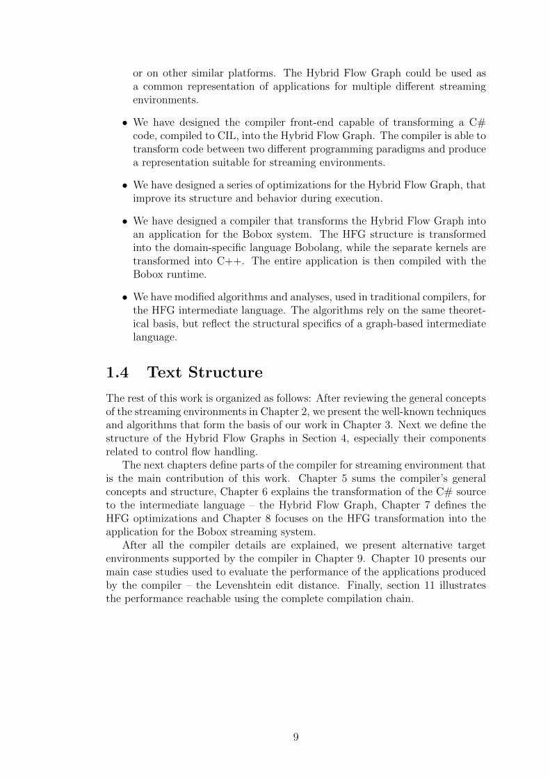
Figure 2.2 shows a simple plan, where we can exploit two kinds of kernelparallelism. First, we can always execute kernels mul and inc in parallel, becausethey are not connected by a stream. Second, we can execute all kernels in parallelfor different values in the input stream. Figure 2.3 shows the kernels executed inparallel for different values of the stream - 1, 2, 3, ... .

Kernel code can be vectorized, because a single kernel is executed on a singleprocessing unit, which is usually equipped with a vector unit (or co-processor),for example SSE or AVX in Intel processors. This unit can be used to parallelizecode inside a single kernel further improving the application performance. Itmight be important to account for the actual number of vector units and theirdistribution between processors, but that is dependent on target platform.

16

load(3)

inc(2)

add(1)mul(2)

Figure 2.3: Kernels executed in parallel for the stream - 1, 2, 3, ...

Bobox prohibits the use of multi-threading inside a kernel, because the pro-duced threads can compete for resources with the Bobox runtime and hinder theoverall performance.

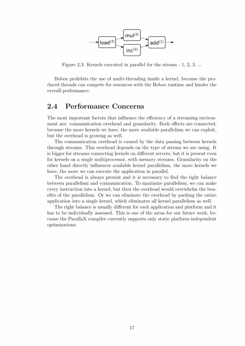
2.4 Performance Concerns

The most important factors that influence the efficiency of a streaming environ-ment are: communication overhead and granularity. Both effects are connected,because the more kernels we have, the more available parallelism we can exploit,but the overhead is growing as well.

The communication overhead is caused by the data passing between kernelsthrough streams. This overhead depends on the type of stream we are using. Itis bigger for streams connecting kernels on different servers, but it is present evenfor kernels on a single multiprocessor, with memory streams. Granularity on theother hand directly influences available kernel parallelism, the more kernels wehave, the more we can execute the application in parallel.

The overhead is always present and it is necessary to find the right balancebetween parallelism and communication. To maximize parallelism, we can makeevery instruction into a kernel, but then the overhead would overwhelm the ben-efits of the parallelism. Or we can eliminate the overhead by packing the entireapplication into a single kernel, which eliminates all kernel parallelism as well.

The right balance is usually different for each application and platform and ithas to be individually assessed. This is one of the areas for our future work, be-cause the ParallaX compiler currently supports only static platform-independentoptimizations.

17

18

3. Common Techniques

In this chapter we provide context on the more complex well known techniquesand systems used in this work. We provide basic description, with small exam-ples, and links to other works that offer more detailed information. The chapterdescribes four important concepts necessary to understand our ParallaX compilerand the examples used in this work: graph rewriting systems in Section 3.1, Kahnprocess networks in Section 3.2, basics of the Common intermediate language codein Section 3.3 and an introduction to the SIMD instructions in Section 3.4.

3.1 Graph Rewriting Systems

A graph rewriting system is a grammar designed to transform graphs [20]. Similarto formal text grammars, the system consists of rules of the form r : L→ R, whereL is the pattern graph and R is the replacement graph [21]. Rewriting systemscan be defined for any type of graph, but in this work, we focus only on orientedannotated graphs, where the annotation is a string.

The semantics and application of the rewriting rules are defined algebraical-ly using either the double-pushout or single-pushout approach. In the double-pushout approach [22], each rule is a pair of graph morphisms, where the firstthe defines nodes and edges to be deleted and the other defines nodes and edgesto be added. In contrast, each rule in the single-pushout approach [23] is repre-sented by a single morphism that applies the transformation in a single pushoutoperation. We use the single-pushout approach, because its rules are simpler andtheir application is more intuitive.

In the case of single-pushout approach, a rule is defined as a morphism r :L→ R, where all the nodes and edges affected by the replacement graph R mustbe matched by the pattern graph L [24]. The pattern graph can contain emptynodes , which do not have specified annotation and can match any node. To makethe semantics and examples more readable, we use a simplified notation, wherewe omit the empty nodes.

cast add add cast add add

Figure 3.1: Simple graph rewriting rules.

Figure 3.1 shows two rewriting rules, the one on the left is a standard graphrewriting rule and the right one is simplified. The nodes without annotation arethe empty nodes that can match a node with any annotation. In the simplifiedrule, we remove the empty nodes and leave only the edges connecting them tosignify where the empty nodes are.

The rules are applied to an input graph one at a time while there is at leastone that matches. The application can be nondeterministic when multiple rules

19

are applicable at the same time. The rewriting system must specify what ruleshould be selected in case nondeterminism, usually according to their order orpriority.

The rule application itself is very intuitive, the matched subgraph is replacedby the replacement. The full theoretical basis of this process is described in detailin the following works [22, 20, 24], but an intuitive understanding is sufficient tofollow the examples.

3.1.1 Associative Graph Rewriting Systems

The original rewriting systems support empty nodes in their pattern graph (Lin rules r : L → R), which can match any node [21]. We had to extend thebasic behavior, because our optimization component requires more control overthe matching process. The associative graph rewriting systems provide enoughcontrol to implement optimizations used in our compiler.

An associative graph rewriting system is a graph rewriting system, wherethe pattern graph can contain group nodes, repeat nodes and chain nodes withbehavior similar to regular expressions.

A group node is defined by a list of allowed annotations, similar to the regularexpression ”[abc]”, where the empty node is basically a special version of thegroup node, equivalent to the expression ”.”.

A repeat node, declared with a + symbol, defines a set of nodes that sharethe same connections but they do not have to be directly connected among them-selves, this construct does not have any regular expression equivalent.

A chain node is defined as ”a∗”, where we require that the repeated nodesare connected as a single string matching the annotation without any outgoingor incoming edges besides the first and last. The rewriting system also allows theuse of special nodes $N in the product graphs, which represent the subgraphsmatched by the group or chain nodes. The behavior is best shown on an example.

cast*

[add|mul]

cast

mul

castldc 8

ret

cast

ldc 1

MATCH$1

REWRITE

ldc+ ldc 5$2$2

Figure 3.2: Regex pattern graph match

Figure 3.2 shows a pattern graph matching an annotated directed graph.The pattern graph contains a group node [add|mul], which matches any nodewith either the add or mul annotation. The empty nodes match a node withany annotation and the chain node cast∗ matches any number od cast nodesconnected one after another. The chain node would not match the graph, if therewas another node connected between the casts. The group and repeat nodes canbe combined, like [add|mul]∗. The repeat node matches any number of ldc nodesconnected to the central group node.

Besides matching the pattern, an associative graph rewriting system must alsoproduces an associative collection connecting the matched and pattern nodes.

20

With it, it is possible to match the pattern and then modify the nodes based onhow they were matched.

3.1.2 Graph Rewriting System Use Cases

We use the graph rewriting systems for multiple different purposes that are notnecessarily connected, besides their graph-based data structures. The work con-tains the following use cases:

Intermediate Language Semantics

We use a graph rewriting system to define the semantics of our intermediatelanguage. The system defines all the operations available in the language and itis part of the language definition.

Source Code Emulation

We developed a graph rewriting system that is able to emulate the calculation ofthe source code (C# code compiled to CIL code) and it is an instrumental partof our data flow analysis. The system is used solely for CIL emulation and hasno relation to the intermediate language.

Optimizations

The optimization component of our compiler is implemented as an associativegraph rewriting system, where each optimization is represented by a single rule.Although the rewriting system modifies the intermediate code, the optimizationcomponent does not change the semantics of the code.

Component Extraction

The component extraction is a special optimization step that groups parts of theintermediate code into bigger, more efficient components. The behavior of eachnew component is defined by the subgraph it represents, we do not add new rulesto the graph rewriting system defining the intermediate language behavior.

3.2 Kahn Process Networks

The Kahn process networks is a distributed model of computation, where inde-pendent serial processes communicate through unlimited serial queues (FIFO)[25]. The processes read and write atomic data elements (tokens) from and tothe queues and they cannot communicate with one another outside of the queues.The entire modeled system is deterministic, despite synchronization and paral-lel execution of the processes. Figure 3.3 shows a small part of a Kahn processnetwork, where the arrows represent queues transferring data and the circles rep-resent processes.

The Kahn process networks were originally designed as a model of compu-tation for distributed systems [26], but they are also used to model embedded

21

p2

p1

p3

Figure 3.3: Part of a Kahn process network

system [27], signal processing [28] and they can be even used to replace streamingenvironments for some applications [29].

The Kahn process networks are similar to the streaming environments, pre-sented in Chapter 2, where processes are an analogy to the kernels and queuesto the streams. Kahn process networks, though purely theoretical, can be con-sidered a subset of streaming environments, because they have similar semantics.The main difference is that the Kahn process networks require processes withdeterministic behavior1, which is not necessary, in the streaming environments.

We do not use the Kahn process networks directly in this work, but the inter-mediate language we designed as part of our compiler satisfies the requirementsand can be considered a KPN. This means that its calculation is deterministicand it does not produce any unpredictable results.

3.3 CIL Basics

We selected the C# programming language as the interface for our ParallaXcompiler, because it is widely known, the language and its entire ecosystem (theCommon language runtime) is standardized [30, 31] and there are advanced utili-ties available for it. Our system processes C# applications compiled to CIL code,which is the intermediate language of the Common language runtime, the processis shown in Figure 3.4. Therefore, a basic understanding of the CIL instructionsand inner workings is useful, because most of the examples used in this work usethe CIL notation or rely on its structure or invariants.

C#

compiler

ParallaX

compilerCIL codeC# code

streaming

application

Figure 3.4: ParallaX compiler interface overview

3.3.1 Common Language Runtime

The Common language runtime, or CLR for short, is and application ecosystem,which allows multiple high level programming languages to be used interchange-ably and platform independently. The infrastructure is standardized under ISOand ECMA [31] and specifies the execution environment, libraries and struc-ture necessary for applications to work. Figure 3.5 shows the CLR architectureoverview.

1The process always produces the same results in the same order for the same inputs.

22

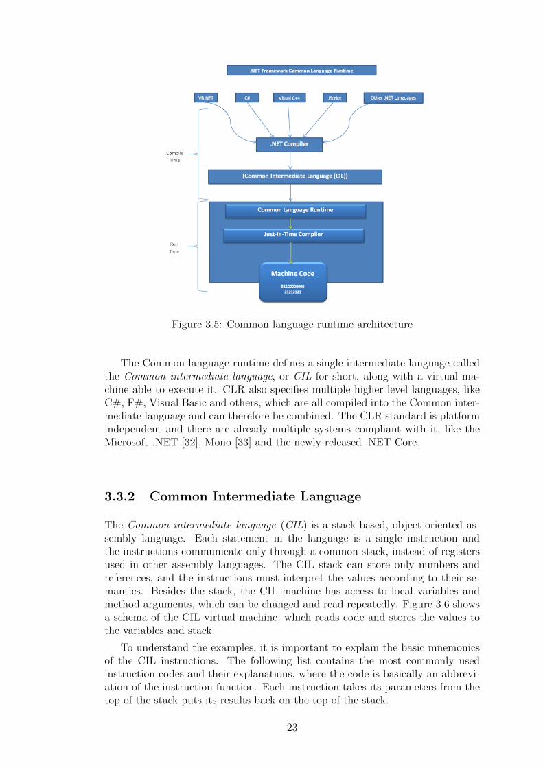
Figure 3.5: Common language runtime architecture

The Common language runtime defines a single intermediate language calledthe Common intermediate language, or CIL for short, along with a virtual ma-chine able to execute it. CLR also specifies multiple higher level languages, likeC#, F#, Visual Basic and others, which are all compiled into the Common inter-mediate language and can therefore be combined. The CLR standard is platformindependent and there are already multiple systems compliant with it, like theMicrosoft .NET [32], Mono [33] and the newly released .NET Core.

3.3.2 Common Intermediate Language

The Common intermediate language (CIL) is a stack-based, object-oriented as-sembly language. Each statement in the language is a single instruction andthe instructions communicate only through a common stack, instead of registersused in other assembly languages. The CIL stack can store only numbers andreferences, and the instructions must interpret the values according to their se-mantics. Besides the stack, the CIL machine has access to local variables andmethod arguments, which can be changed and read repeatedly. Figure 3.6 showsa schema of the CIL virtual machine, which reads code and stores the values tothe variables and stack.

To understand the examples, it is important to explain the basic mnemonicsof the CIL instructions. The following list contains the most commonly usedinstruction codes and their explanations, where the code is basically an abbrevi-ation of the instruction function. Each instruction takes its parameters from thetop of the stack puts its results back on the top of the stack.

23

CIL

virtual

machine

add

ldl a

ldc 0

stl a

...

324

5

...

Stack

Code10p

......

324a

......

Local variables Parameters

Figure 3.6: CIL virtual machine

• ldc – load constant written directly in the code

• ldarg, starg – load argument, store argument

• ldloc, stloc – load local variable, store local variable

• mul, add, div, ... – arithmetical operations (multiply, add, divide, ...)

• blt, bge, ... – conditional jumps (brunch less than, branch grater than, ...)

• ret – return method result

The CIL instruction set contains specialized instruction versions defined bysuffixes. For example ldc.i4 0 is an instruction that loads zero to the stack as afour-byte integral number. There is also ldc.i8 0 and ldc.r8 0, for an eight-byteinteger and a double precision floating point number. We usually omit thesespecialized versions, because they specify data types and we store data typesseparately.

Aside from the data type specialization, there are also short version of instruc-tions that access first few parameters and local variables. These instructions havethe suffix identifying the index of the variable or argument, like stloc.0 that storesa value into the first local variable and is the short version of the stloc C instruc-tion for the code in Listing 3.1. The most commonly used short instructions areldloc.N , stloc.N , ldarg.N , starg.N and ldc.N , where N represents the constantvalue.

Listing 3.1 shows a minimum function implemented in C# as a static methodand Listing 3.2 shows the same method compiled into CIL. The CIL code containsonly the instructions listed above and we added comments that help separateparts of the code to better match it to the original C# code.

24

public stat ic int minimum( int A, int B){

int C;i f (A < B)

C = A;else

C = B;return C;

}

Listing 3.1: Minimum method implemented in C#

3.4 SIMD Instructions

The principles of the vector instructions are important for the algorithm structureand in this section, we revise the instructions and memory model fundamentalswith particular emphasis on the aspects important for the studied problem. Wewill explain vectorization on the Intel / AMD SIMD extensions, mainly SSE.

3.4.1 Vectorization

The Streaming SIMD Extensions (SSE) is a vector instruction set extension tothe x86 and x64 architecture, designed by Intel and introduced in 1999 as a suc-cessor to the older MMX extension. SSE provides new instructions that performvector calculations on 128 bit vectors, stored in newly added registers. SIMDinstructions can increase performance for algorithms that can keep the data inthe special registers and perform multiple instructions before moving then backinto the memory. The SSE instructions follow the Single Instruction MultipleData or SIMD model, where a single operation is applied to all elements of avector at once.

The original SSE was updated to SSE2 and SSE3, with each adding newinstructions, and introducing new data types available in the 128 bit vectors.The original SSE supported mostly single precision floating point numbers andthe later versions added double precision and integral numbers of differing sizes (8,16 and 32 bits). The SSE extension was further expanded by the AVX and AVX2expansions adding 256 bit vectors and new instruction and AVX-512 introducing512 bit vectors.

The vector instructions have similar requirements as the GPU, which wasthe original target platform for the blocked Levenshtein distance algorithm. Thesimilarities allow us to adapt the algorithm for our compiler without fundamentalchanges.

3.4.2 SIMD Instructions Types

SSE and its updates provide vector instructions similar to the arithmetic in-structions available in CIL, but instead of a single number the instructions vorkwith a whole vector of values. The SIMD instructions are divided into multiplecategories:

• Arithmetic operations – instructions that perform the vector calculations.

25

. method public h idebys i g stat ic i n t32 minimum (int32 A, in t32 B) c i l managed

{. maxstack 2. l o c a l s i n i t ( [ 0 ] in t32 C )

// i n i t i a l i z a t i o n o f C to 0IL 0000 : ldc . i 4 . 0IL 0001 : s t l o c . 0// i f c o n d i t i o n (A < B)IL 0002 : lda rg . 0IL 0003 : lda rg . 1IL 0004 : bge . s IL 000a// t r u e branch (C = A; )IL 0006 : lda rg . 0IL 0007 : s t l o c . 0IL 0008 : br . s IL 000c// f a l s e branch (C = B; )IL 000a : lda rg . 1IL 000b : s t l o c . 0// re turn CIL 000c : l d l o c . 0IL 000d : r e t

} // end o f method FlowGraphTest : : minimum

Listing 3.2: Minimum method defined in Listing 3.1 compiled to CIL

26

• Logic operations – instructions that perform logical operations on the vectorvalues.

• Memory management – instructions that transfer the data from or to thememory.

• Shuffle operations – instructions that efficiently exchange data in the vectorregisters.

• Miscellaneous – additional instructions for initialization and configurationof the SIMD unit.

The arithmetic operations are further categorized based on the data type theysupport. Each instruction interprets the registers as a vector of different valuesand using incompatible instructions can lead to invalid values.

3.4.3 Memory Organization

The original SSE supported eight new 128 bit registers which was extended tosixteen with the introduction of the 64-bit architecture. The AVX extensionadded sixteen new 256 bit registers. These registers are dedicated to the vectorextensions and they are not available to the CPU for standard instructions.

The vectors must be filled by special SSE or AVX instructions, which eithermove data from memory or fill the vector with a constant. Moving data to theregisters can be costly operation, especially when performed frequently. Theapplications should reuse the data in registers as much as possible, which meansthat any compiler producing the SIMD instructions must keep the live variables[4] in the registers while they are needed.

The memory transfers to the SSE registers are limited to the data aligned to16 bytes 2. The unaligned data can be transfered as well, since SSE2, but thetransfer is much slower than for the aligned data. To mitigate this effect, theParallaX compiler produces code that automatically allocates all the vector dataaligned to 16 using a custom memory manager.

3.4.4 SIMD in C++

The SIMD instructions are accessed via intrinsic functions provided by the C++compiler or its library. The intrinsics are provided as simple functions, where eachinternally represents a single SSE or AVX instruction, and each call is replaced bythe instruction (inlined). The ParallaX compiler produces C++ code containingthe intrinsic functions and the C++ compiler produces the final code with theSIMD instructions.

The special registers are represented by special data types, like the m128itype representing four 32 bit integers. The registers are used by declaring avariable of the data type.

2Address is divisible by 16

27

28

4. Hybrid Flow Graph

The Hybrid Flow Graph, or HFG for short, is a compact format designed forrepresentation of procedural code with operational semantics similar to the be-havior of streaming systems. All the data types, control flow and data flow arerepresented by a single graph, unlike the control-flow graphs [35] and data-flowgraphs [36] constructed by the traditional compilers, where each graph representsa single aspect of the processed code. The HFG definition is platform specific;nevertheless, the construction of the graph is a general algorithm that can beadapted for many platforms (intermediate codes).

A Hybrid flow graph is an annotated directed graph, where nodes togeth-er with their labels represent operations and edges define data transfers. Theorientation of the edge indicates the direction of data flow and the edge annota-tion defines the data type transported along the edge. The complete list of allsupported operations and data types is part of the HFG definition.

The HFG defines two sets of operations necessary to represent both the CILsemantics and control flow structure. The first set of operations is borrowed fromthe underlying environment, the CIL standard [30]. These operations are deriveddirectly from the CIL instructions and we call them the basic operations . Thesecond set contains the special operations that model the control flow structure,their semantics are defined in detail in Section 4.3.

The data types supported by the HFG edges are taken from CIL standard[30] and we add a single new data type called Token, which represents elementswithout value used to initialize the HFG nodes.

Figure 4.1 shows an example Hybrid flow graph implementing the factorialfunction defined in Listing 4.1. The graphical notation introduced in this sampleis carried over to the other examples. The graph nodes represent:

int f a c t o r i a l ( int a ) {int b = 1 ;do {

b = a ∗ b ;a = a − 1 ;

} while ( a > 1 ) ;return b ;

}

Listing 4.1: Method containing a single loop

29

• basic operations – rounded rectangles inscribed with instruction codes

• start special operation – squares inscribed with I

• return special operation – squares inscribed with R

• parameter special operation – squares inscribed with P and parameter name

• merge special operations – squares inscribed with M

• split special operations – squares inscribed with S

• loop primer special operations – squares inscribed with L

• broadcast special operations – filled squares without inscription

• input special operations – circles inscribed with number

The special operations represent control flow and data distribution, they aredefined later, in Section 4.3. The input operations represent specific input forother operations, especially for those with more than one, we omit them foroperations with a single input to make the examples more compact. The datatypes of the edges are defined by their graphics as follows:

• integer – solid lines

• boolean – dashed lines

• Token – dotted lines

M L

S

3

1

2

1

2

1 2

bgt

ldc 1sub

1

2

1 2

M

S

3

1

2

1

2

ldc 1

ret

mul

1

2

Pa I

R

Figure 4.1: The HFG representation of the factorial function

30

4.1 Related Work – Hybrid Flow Graph

We designed the Hybrid Flow Graph (HFG for shot) as an intermediate languagecapable of representing procedural applications across various streaming environ-ments in a form similar to the structure of their native applications. The HFGis a graph-based declarative language that uses operators defined according tothe CIL instructions and it is defined along with a compiler able transform C#code into the HFG. The final structure of the Hybrid flow graph was presentedin our work [1], where we defined the graph structure, semantics and construc-tion. The original theoretical basis was formulated in our previous work [5], butthe graph was further refined to accommodate all the features necessary for coderepresentation and efficient execution.

The Hybrid Flow Graph described in this work is similar but not identical toother modeling languages, like Petri nets [39] or Kahn process networks [40]. Themain difference is that the HFG was designed for automatic generation from thesource code, where the other languages are generally used to model the applicationprior to implementation [41] or to verify a finished system [42].

The Hybrid Flow Graph is not only a compiler data representation, it is a pro-cessing model as well, similar to KPN graphs [43]. It can be used as a source codefor specialized processing environments, where frameworks for pipeline parallelismare the best target, since these frameworks use similar models for applications[44]. One such a system is the Bobox framework [2], where the flow graph can beused to generate the execution plan similarly to the way Bobox is used to executeSPARQL queries [45].

The Hybrid Flow Graph is closely related to the program dependence graph(PDG), which can be also used to represent procedural code [46]. The programdependence graph was designed for traditional procedural languages, like For-tran, where the graph construction relies on the source code statements. Modernlanguages, like C#, provide far more complex source code syntax and their directtransformation into a graph is impractical, since it means replicating the C#compiler to parse the code. To offset the complexity, we transform the CIL code,which is more simple. The main cost of this approach is increased granularity ofHFG compare to the PDG, which we reduce lated using optimizations.

The flow graph has similar traits to frameworks that allow applications to begenerated from graphs, like UML diagrams [47] [48], but we concentrate on graphextraction from procedural code, which is more convenient for the design of dataprocessing application.

The flow graph semantics is defined using the graph rewriting system [49],which can be used to design and analyze applications, but it is not convenient forexecution. The graph rewriting systems continuously modify the graph structure,which severely limits optimization. There are other frameworks that generategraphs rewriting systems from procedural code like Java [50], but the producedsystems are inconvenient for efficient execution and we use them solely to definethe graph semantics.

Since the global determinism of our flow graphs is ensured by the generator,the Hybrid Flow Graph has more relaxed local constraints than a KPN, butstill more stringent than a Petri net. There are frameworks which are able toconstruct KPN graphs from simple programs [51], but the flow graph contains

31

more information about the source code and it is designed for data processingapplications.

The Hybrid Flow Graph is closely related to graphs used in compilers, mainlythe dependence and control flow graphs [36], where the HFG merges the infor-mation from both. The construction of a HFG and its subsequent optimizationis related to well-known compiler techniques, like points-to analysis [52], depen-dence testing [35] and control-flow analysis [53]. In compilers, graphs resultingfrom these techniques are typically used as additional annotation over intermedi-ate code. On the contrary, our Hybrid Flow Graph contains complete informationand, thus, it is an intermediate code representation in itself.

The close relationship to the data-flow (dependence) [36] and control-flowgraphs [54] is natural, because together they represent the two most importantaspects of the procedural code. However; it is not possible to use either of thegraphs alone to fully represent an application, because each lacks some informa-tion about the code. The control-flow graph does not define data connectionsand the data-flow graph is not deterministic. One approach would be to combineboth graphs into one, but that generally leads to a graph with an exponentialnumber of nodes relative to the size of the original code.

4.2 Basic Operation Semantics

We use graph rewriting systems [48] to define the semantics of operations, whichis the approach we used in formal definition of the HFG semantics [6]. We usethe graph rewriting systems only as a theoretical tool, because the real imple-mentations work as streaming systems rather than graph rewriting systems.

To properly define the semantics of the Hybrid flow graph we add a thirdset of operations, the data operations . Nodes annotated with these operationsrepresent values processed by the HFG during execution and they do not performany actual work. We show the data operations as elliptic nodes in the examples.

The data operations are introduced, because the edges represent streams in thestreaming systems, but the pure graph representation provides no mechanism toimplement this behavior. Instead we chain data as nodes where otherwise wouldbe a stream. These operations are used only to define the semantics and theyare not used in the actual implementation, because there, the edges representstreams that store the processed value.

First, we define the semantics of the basic operations based on the CIL in-structions. The semantics are defined according to the CIL standard [30], wherethe consumed and produced values are taken from the input and output streamsinstead of the common stack or variable memory. It is the responsibility of thecompiler to construct the graph so that the edges represent the connections thatthe stack provides in the original CIL.

Figure 4.2 defines the semantics of a few select CIL instructions, where theelliptic nodes represent the data operations and the ∗ represents an empty token.We do not show the definition of all the instructions, because it is straight forward,the instruction consumes data and produces the results from and to the edges.

The only special case are the branch instructions (like bgt in Figure 4.2) whichnormally move the program counter. In our semantics they just produce a boolean

32

ldc x ldc x add add

1 2 1 2

bgt bgt

x y

x+y x>yx

* 1 2 1 2

x y

Figure 4.2: Semantics of load constant, add and compare (<)

value that says whether the jump should happen or not and the actual control flowmanagement is handled by the special operations described in the next section.

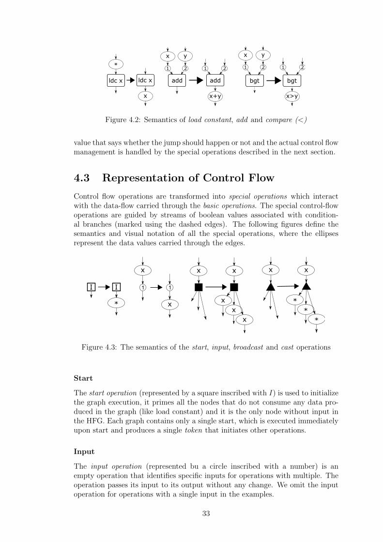
4.3 Representation of Control Flow

Control flow operations are transformed into special operations which interactwith the data-flow carried through the basic operations. The special control-flowoperations are guided by streams of boolean values associated with condition-al branches (marked using the dashed edges). The following figures define thesemantics and visual notation of all the special operations, where the ellipsesrepresent the data values carried through the edges.

x

I I

*

x

x

x

x

x

x

x x

*

*

*

Figure 4.3: The semantics of the start, input, broadcast and cast operations

Start

The start operation (represented by a square inscribed with I) is used to initializethe graph execution, it primes all the nodes that do not consume any data pro-duced in the graph (like load constant) and it is the only node without input inthe HFG. Each graph contains only a single start, which is executed immediatelyupon start and produces a single token that initiates other operations.

Input

The input operation (represented bu a circle inscribed with a number) is anempty operation that identifies specific inputs for operations with multiple. Theoperation passes its input to its output without any change. We omit the inputoperation for operations with a single input in the examples.

33

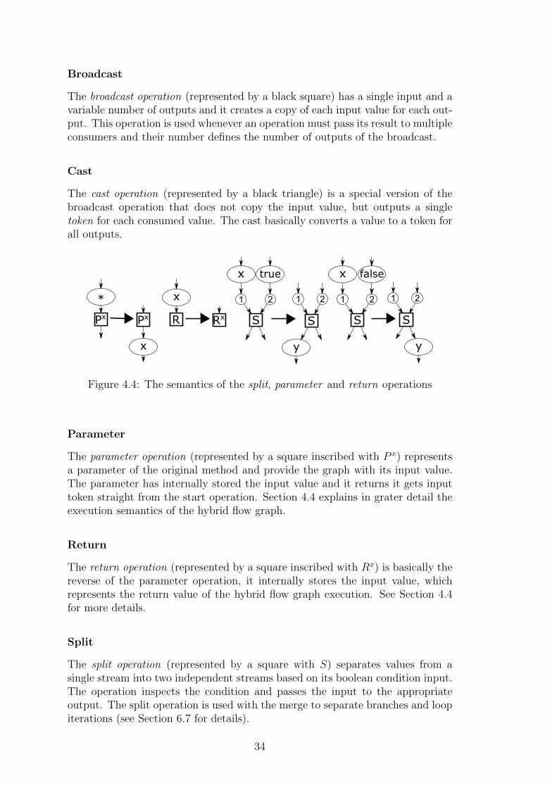
Broadcast

The broadcast operation (represented by a black square) has a single input and avariable number of outputs and it creates a copy of each input value for each out-put. This operation is used whenever an operation must pass its result to multipleconsumers and their number defines the number of outputs of the broadcast.

Cast

The cast operation (represented by a black triangle) is a special version of thebroadcast operation that does not copy the input value, but outputs a singletoken for each consumed value. The cast basically converts a value to a token forall outputs.

S S

falsex

y

S S

truex

y

Px

*

Px

x

R

x

Rx

Figure 4.4: The semantics of the split, parameter and return operations

Parameter

The parameter operation (represented by a square inscribed with P x) representsa parameter of the original method and provide the graph with its input value.The parameter has internally stored the input value and it returns it gets inputtoken straight from the start operation. Section 4.4 explains in grater detail theexecution semantics of the hybrid flow graph.

Return

The return operation (represented by a square inscribed with Rx) is basically thereverse of the parameter operation, it internally stores the input value, whichrepresents the return value of the hybrid flow graph execution. See Section 4.4for more details.

Split

The split operation (represented by a square with S) separates values from asingle stream into two independent streams based on its boolean condition input.The operation inspects the condition and passes the input to the appropriateoutput. The split operation is used with the merge to separate branches and loopiterations (see Section 6.7 for details).

34

M M

truex

x

M M

falsex

y

Figure 4.5: The semantics of the merge operation

Merge

The merge operation (represented by a square with M) combines two inputstreams into a single output stream according to a boolean condition input stream.The operations first inspects the condition value and then passes the appropriatevalue from one of the input streams to the output stream, one input contains thevalues for the true condition and the other for false.

true

true

false

false

L L L L L L

*

Figure 4.6: The semantics of the loop primer operation

Loop Primer

The loop primer operation (represented by a square with L) it the only operationwith two states. The operations first reads its first input and returns false, thenit reads its second input while it is true and returns true. When the secondinput is false, the loop primer returns to the initial state (reads first input). Thisoperation is used with split and merge to control loop iterations, because the loopbody must first consume data produced prior to the loop and than it consumesdata produced in the previous iterations.

4.4 Hybrid Flow Graph Execution

The hybrid flow graph is an intermediate language that is not meant to be ex-ecuted by itself, it is further transformed into a streaming system application,but it is still beneficial to fully define its execution semantics. The hybrid flowgraph operational semantics is defined by the graph rewriting system presented

35

in the previous sections, but an actual execution (even if theoretical) still requiressimple preparation.

The HFG is defined and constructed so that there is a single node withoutinput that initialized the entire graph. This means that the parameters mustbe filled into the graph before it is executed, we call this step the instantiationand it requires that all parameters are annotated with their actual values. Nextwe apply the rules of the graph rewriting system, while there is at least oneapplicable, we named this phase evaluation. And finally we extract the result inan operation we call reduction, where we get the value from the return operation.The process is defined in Algorithm 1.

add

Pa Pb

R

I

1 2

add

P3 P5

R

I

1 2

add

P3 P5

R

I

1 2

add

P3 P5

R8

I

1 2

add

P3 P5

R8

I

1 2

instantiate

(a=3, b=5)

evaluate reduce

8

Figure 4.7: Hybrid flow graph execution example

The actual execution can be illustrated on a small example. Figure 4.7 showsa graph that adds the value of two parameters and returns the result. Thefigure shows all three steps of the HFG execution – instantiation (with parametervalues), evaluation and reduction (producing the result).

Algorithm 1 Hybrid flow graph execution

Require: G – hybrid flow graphGRS – graph rewriting system defining HFG semanticsP – set of all the parameter values

Ensure: X – return valueGI := instantiate(G,P )R := r ∈ GRS : applicable(r,GI)while R 6= ∅ dor := first(R)GI := r(GI)R := r ∈ GRS : applicable(r,GI)

end whileX := reduce(GI)

4.5 Layered Hybrid Flow Graph

The hybrid flow graph definition is based on the CIL instructions, which meansthat the graph is generally large and granulated, which can cause inefficiency in

36

the final streaming application. We designed a transformation called componentextraction to offset this effect.

The component extraction takes select parts of the graph and combines theminto a single operation with equivalent semantics. In practice, this would requireadding new operations and their semantics into the hybrid flow graph languagedefinition, which would be impractical.

We define a extended version of HFG to allow the components to be defineddirectly by their original subgraph. A layered hybrid flow graph is a hybrid flowgraph which can contain custom operations that have semantics defined by an-other hybrid flow graph.

custom

Pa

Pb

RI

1

2

mul1

2add

2

11

2

custom

Figure 4.8: Layered hybrid flow graph example

Figure 4.8 shows a small hybrid flow graph with a custom operation definedby another graph that adds and multiplies its two inputs and returns a singlevalue.

37

38

5. Compiler for StreamingEnvironments

The design of applications for streaming environments can be complicated andrequires specific knowledge of the environment and sometimes even the underlyinghardware. We discussed the specifics in Section 2.2.

The goal of this project is to make the design of applications for streamingenvironments simpler and more efficient. To accomplish this, we have designedthe ParallaX compiler that allows developers to design entire applications ortheir parts in a common procedural language, we selected C# for its wide spreadknowledge and well documented intermediate code. Developers simply createan application in C# and our compiler transforms it for a supported streamingenvironment. We currently support multiple parallel environments, but we mainlyfocus on a native implementation of the Bobox [2] streaming environment. Theother supported environments are specified in Section 8.2.

5.1 Related Work – Intermediate Code and

Parallelism

The ParallaX compiler was designed to simplify the development of applicationsfor the Bobox streaming system, its structure is based on our work [1], where wedefined the compiler architecture and the compilation process. The theoreticalbasis of the entire system is based on our previous work [7], where we presentedthe basic concepts of the Hybrid Flow Graph and its construction.

Compilers of procedural programming languages traditionally use interme-diate code separated into two layers – the control flow and the data flow, theformer being a graph of basic blocks while the latter assigns either a sequence ofinstructions or a data-flow graph to each basic block. This textbook approach[57] has become standard whenever the target machine is a CPU which possesdirect representation of the control-flow instructions. Data-flow graphs in com-pilers are usually limited to individual basic blocks – this limitation guaranteesacyclic structure of the data-flow graphs (named dags therefore) which in turnallows simpler semantics and easier handling.

Attempts to integrate the control-flow and data-flow levels of intermediatecode occurred throughout the decades of development of compilers, the mostsuccessful being probably the Program Dependence Graph (PDG) [46] used re-cently in compilers for GPU architectures [58]. Nevertheless, the PDG is only anannotation over the underlying sequential code and modern compiler ecosystemslike LLVM still rely on intermediate codes based on instruction sequences.

Different representations are used in hardware synthesis where the result ofcompilation is not a code but an electronic circuit [59]; however, the source lan-guage SystemC, although originated from C, was significantly changed towardsthe hardware definition domain; consequently, the language as well as the prin-ciples of compilation are not easily applicable to general programming.

Synthesis of electronic circuits has been the main motivation for data-flow

39

representations of procedural code; nevertheless, intermediate codes and conver-sion algorithms targeted at general computing appeared both in the history [60]and present times [61], sometimes suggesting a new hardware architecture as thetarget platform [62]. Since conversion of low-level languages like C++ is difficultdue to aliasing problems, some conversion algorithms require hints in the form ofannotations added to the procedural source code [63, 64].

Although none of the suggested approaches reached wide recognition yet, thecurrent success of high-level data-flow architectures like TensorFlow suggests thatdata-flow orientation may be a viable alternative to von-Neumann architectures.

In the environment of modern languages like C# or Java, there already wereseveral alternate intermediate codes introduced. Of particular importance to ourapproach are systems similar to graph-rewriting systems, like the one described forJava [50]. Java was also subject of numerous approaches to vectorization [65, 66]or parallelization [67, 68]. Parallelization often makes use of additional user-inputthrough the use attributes or other ways of annotation [69, 70]. Another techniquewhich shares some similarity with stream-based processing was described in [71].

There are also works focusing on the parallelization of dynamic languages,mainly used for web content production or scripting, like JavaScript, PHP andPython. JavaScript can efficiently take advantage of the parallel capabilities ofHTML5 [72], or there is the possibility to employ even more powerful technologieslike OpenCL [73]. The parallelization of PHP is one potential goal of the Peachpiecompiler [74]. All the previous works focus mostly on loop parallelization orvectorization and cannot be directly adapted for streaming systems, but theyshow that the dynamic languages can be adapted as an interface for parallelsystems.

5.2 Compiler Architecture

We have designed a compiler that takes a C# application compiled to CIL andtransforms it to an application for a streaming environment. We call it theParallaX compiler . The compiler mostly follows the standard architecture shownin Figure 5.1, where we omit only the platform specific optimizations as they areperformed by the streaming environment and the C++ compiler associated withit.

The architecture in Figure 5.1 is designed for a direct transformation, sourcecode to a machine / binary / byte code, but streaming environments require planand operations, not just a single code. Therefore; our compiler requires some non-standard parts and a special intermediate language better suited for streamingenvironments. The structure of our compiler is shown in Figure 5.2. We havedesigned a special intermediate language with platform independent structureand semantics well suited for streaming environments. We named this languageHybrid flow graph, or HFG for short, and it allowed us to adapt our compiler formultiple target platforms besides just native Bobox. The language was describedin detail in Chapter 4.

Figure 5.2 shows the architecture of the ParallaX compiler with its componentsgrouped into the three main parts – front-end, optimization and back-end. Thecompilation process is explained in the following chapters, but the basic idea isstraight-forward: the CIL instructions are transformed into the graph nodes and

40

Figure 5.1: Standard compiler architecture overview taken from the book Com-pilers: principles, techniques, tools [57]

C#

source code

CIL code

HFGC#

compiler

Graph

construction

Component

extraction

Code

generation

Global

HFG

Layered

HFG

Runtime

environment

Plan

generation

front-end optimization back-end

Figure 5.2: Compilation and code generation

connected by edges, representing data transfers, created according to the data andcontrol flow. The instructions are then grouped based on the graph structure tocreate kernels (basically complex instructions) for the streaming environment.The data transfers between the operations from the execution plan, because theydefine how the operations are executed and how they interact.

The first part of our compiler is the front-end, where the code of a singleprocedure, usually the main method, is transformed into a hybrid flow graph.The input of our compiler is a C# code compiled into a CIL code by a C#compiler. Chapter 6 describes all the steps necessary to create a HFG equivalentto the input code.

Next, the graph is transformed into a layered hybrid flow graph, defined in Sec-tion 4.5. This step is called optimization, because it reduce the graph granularityand improves the efficiency of the final application. The process is explained indetail in Chapter 7.

Last part of the compiler is the back-end, where we take the layered graph andtransform the top layer to the execution plan for the streaming environment andthe rest we transform into C++ code implementing the custom operations. The

41

back-end is platform specific, depending on the target environment, we discussthe available versions in Chapter 8. The produced application is then processedby the runtime environment and executed.

5.3 Input Language Restrictions

A compiler must always produce a valid code, which means that it has to bevery conservative when it encounters constructs that do not follow a patternthat allows for optimization. This is especially important for a compiler thattransforms the code between two very different platforms, like the object-orientedC# and streaming environments.

The structure of the streaming environments is significantly different fromthe object-oriented environment of the CLR and C# and we impose restrictionson the applications the ParallaX compiler is able to process. Without the re-strictions, the produced code would be too inefficient or the application mightbe impossible to compile. The ParallaX compiler does not currently support thefollowing constructs:

• objects – the compiler supports only static methods, which can call otherstatic methods.

• multi-dimensional arrays – we support one-dimensional arrays, but it ispossible to represent multi-dimensional arrays in one-dimensional arrays.

• exceptions – exceptions and guarded blocks are not allowed, errors can bereported by returning invalid values.

• libraries – library methods and classes are not supported, because we donot have access to their code (in case of native implementation) and theydo not have equivalent in streaming environments. In the future, we willprovide special library compatible with the streaming environments.

• switch – the compiler supports only if-else, but switch support will be addedin the future.

• break, continue and goto – we do not allow these constructs, because theycan abruptly interrupt the control flow in a way that is not possible instreaming environments.

This work is a proof-of-concept and the purpose of the ParallaX compiler isnot to parallelize arbitrary C# applications, but to provide another interface forthe streaming environments to developers without specific domain knowledge ofthe systems. However; the compiler can be further improved to incorporate someof the restricted concepts.

Switch can be added with slight modifications to the compiler, because it canbe represented by a series of if-else branches already supported by the compil-er. Custom libraries must be implemented, but there is already a small libraryintegrated with the compiler that can be used as an example.

Break, continue and goto cannot be simple introduced, because the streamingenvironment lack the means to replicate their behavior. It might be possible to

42

add break and continue by restructuring the respective loops, but a general gotocannot be added as it can change the control-flow too significantly.

Multi-dimensional arrays can be added as well, but they would introduce com-plex aliasing and their efficient handling would require advanced optimizations,which are currently not implemented.

Value object types (structs) can be added with proper handling. They do notintroduce aliasing, because they do not have reference semantics. Their integra-tion could be achieved in a similar way as single-dimensional arrays, described inSection 6.9.

Objects and exceptions cannot be fully supported, because they do not haveany equivalents in the streaming environments. Exceptions can unpredictablychange the execution order and modify the application state and there is no wayto do that in a streaming system, which is driven by data. Objects along withthe garbage collector can be also very unpredictable and they introduce aliasing,which could severely limit available parallelism.

43

44

6. Compiler Front-end

Figure 6.1 shows the overview of the HFG construction process. Our input isa CIL assembly compiled from a C# code. The original C# code is compiledusing Microsoft cs to CIL and packed to an assembly (library or executable) byMSBuild. The resulting CIL assembly is analyzed and directly transformed byour compiler to the final Hybrid flow graph.

6.1 Front-end Overview

The compiler transforms a single procedure to a streaming application, whichusually means the main method of the C# application. Aside from the compileritself, we provide also a small library of attributes that allow users to specify otherprocedures for transformation and they can also modify the way it is carried out,used optimizations and generated outputs.

The basic idea of the HFG construction is to transform all the CIL instruc-tions to graph nodes and connect them according to data and control flow. Wecreate a set of basic nodes, each representing a CIL instructions. Then we addspecial nodes based on control flow analysis completing the HFG, which repre-sents the entire input code (procedure or application). A complete HFG is latertransformed to plan for a streaming environment or another parallel system. Fi-nally, we optimize the complete HFG to better balance overhead and availableparallelism.

General parallelization approach is to analyze the source code and locate cer-tain patterns or dependences to find opportunities for parallelism. We use areverse approach, we transform the application to the HFG directly and then weoptimize the resulting graph by merging instruction nodes wherever it is benefi-cial.

C#

source code

CIL code

HFGC#

compiler

Procedure

selection

front-end

Procedure

integration

CIL

preprocessor

Data-flow

analysis

Control-flow

analysis

Instruction

classifier

CIL

procedure

CIL procedure

(without calls)

CIL

instructions

Annotated

instruction

stream

Reaching

definitions

Figure 6.1: Overview of the ParallaX compiler front-end component

Figure 6.1 shows the front-end structure with the two main parts being: thedata-flow and control-flow analyses. The data flow analysis is similar to thereaching definitions analysis [75], but we calculate it using a graph rewritingsystem emulating the CIL code behavior. The control flow analysis is based on acontext-free grammar and parser generator commonly used in standard compilers.

45

The compilation starts with three preparation steps that produce a singleCIL instruction list that is then transformed into a HFG by the data-flow andcontrol-flow analyses. The preparation steps are: the procedure selection, theprocedure integration and the CIL preprocessor. The algorithms are described inSection 6.3, Section 6.4 and Section 6.5 respectively.

We use the data-flow analysis to locate all producers and consumers for eachinstruction, we describe the process in Section 6.6. The data-flow analysis pro-duces a set for each instruction that contains all the instructions that consumea value produced by the instruction, basically a set of all consumer. The outputis similar to the result of the reaching definitions analysis , which locates all thevalues able to reach each statement [75].

The instruction classifier categorizes the instructions according to their con-trol flow behavior: conditional and fixed jumps, jump targets and standard in-structions. The process is described in Section 6.6.5.

The control-flow analysis takes the output of both the data-flow analysis andthe instruction classifier and constructs the final hybrid flow graph. The control-flow analysis locates the control flow constructs (loops and branches) and foreach construct, the analysis produces its body and connects it to the entire graphusing special operations. The non-jump instructions are transformed to basicoperations and connected to the graph.

CIL code represents control flow as a set of conditional jumps. However, weanalyze the CIL code produced by the Microsoft C# compiler, which transformscontrol flow into a well defined structure of jumps. We reconstruct the controlflow based on that structure. This approach does not support general CIL code,but it is sufficient for a CIL generated from a C# source code, which is our targetplatform.

6.1.1 Transformation Example

We will illustrate the entire transformation process on a single example to providea more coherent insight into each step. Listing 4.1, from the previous chapter,contains a C# source code of the factorial method and Listing 6.1 contains theCIL code produced by compiling the C# source. Figure 4.1 shows the com-plete HFG created from the CIL code using the algorithms described in the nextsections and throughout this chapter, we will construct the graph step-by-step.

6.2 Related Work – Compiler Front-end

The compiler front-end is responsible for the transformation of a source code intoa more manageable intermediate language, which is either simpler, more efficientor similar to the target environment. The textbook solution contains a seriesof analyses that explore the aspects of the source code and provide informationabout its structure for the intermediate code construction or further optimizations[57].

The front-end of our compiler follows the standard solution – we constructthe Hybrid Flow Graph (intermediate code) from a C# code, compiled into CILcode by a standard C# compiler (source code). To properly construct the HFG,

46

Listing 6.1: CIL code created from C# code in Listing 4.1

. method private stat ic i n t32 f a c t o r i a l ( in t32 a ){

. maxstack 2

. l o c a l s i n i t ( [ 0 ] in t32 b)

IL 0000 : ldc . i 4 . 1IL 0001 : s t l o c . 0// loop s t a r t ( head : IL 0002 )

IL 0002 : lda rg . 0IL 0003 : l d l o c . 0IL 0004 : mulIL 0005 : s t l o c . 0IL 0006 : lda rg . 0IL 0007 : ldc . i 4 . 1IL 0008 : subIL 0009 : s t a r g . s aIL 000b : lda rg . 0IL 000c : ldc . i 4 . 1IL 000d : bgt . s IL 0002

// end loopIL 000 f : l d l o c . 0IL 0010 : r e t

} // end o f method Program : : F a c t o r i a l

47

we require three main analyses: the data-flow analysis, the data type analysis andthe control-flow analysis.

Before we apply the aforementioned analyses, we must address the procedurecalls present in the source code. The procedure calls limit our ability to safelyconstruct the Hybrid Flow Graph structure and this is especially problematicwith procedures where we do not have access to their source code. To eliminatethis problem, we limit the use of C# standard library, instead; we provide ourown library that contains procedures known to the compiler. We use procedureintegration (also known as inlining) [76], which reduces the source code into asingle procedure without any additional calls [1]. The integration is commonlyperformed by the CIL runtime to produce more efficient code [77], but we haveto perform the integration ourselves since we work with the CIL code directly.

The data-flow analysis is responsible for mapping producers and consumersfor all potential variables. The analysis creates a set of producers and consumerfor each CIL instruction, so we can properly connect the graph nodes based onthem. The concept is very similar to the reaching definitions analysis [75], wherewe use a more dynamic solution to gather additional information about the codebehavior. We statically emulate the source code to analyze the data-flow, datatypes of values and most commonly used control-flow paths. The concept issimilar to the optimizations based on runtime behavior of the application or aprofiler [78].

The compiler accepts CIL code as the input for the front-end, which is astrongly typed language. Therefore; we are not subject to the undecidable da-ta types commonly encountered in dynamic languages, like PHP [79]. The CILstructure still allows for implicit and explicit conversion [31], which can seriouslylimit the performance of the resulting applications, because it might lead to con-stant vector conversions. We analyze the data types during the data-flow analysisand assign a strict type constraint to each edge of the resulting HFG [1].

Another common problem of the object-oriented languages is aliasing , whichis usually addressed by the points-to analysis [80]. We do not have to addresscomplex aliasing, because we forbid the use of object types in the source code,with the exception of the arrays. In the Hybrid Flow Graph produced by the front-end, the nodes always exchange complete arrays and modify them locally beforepassing them on. This inefficient behavior is later addressed by the optimizations,which optimize only arrays that are not aliased in the relevant context, where weuse a process similar to the live variable analysis [4].

The control-flow analysis must determine the order in which the instructionsare processed in the source code and we use this information to properly mergethe HFG edges, representing data transfers. Our implementation follows thepattern similar to the process of basic blocks extraction [54]. We use a pushdownautomaton, commonly used in syntax analysis [57], to analyze the control-flowand we construct the Hybrid Flow Graph in the process (according to the resultsof the previous analyses).

6.3 Method Selection

The first preparation step must select methods, which will be transformed intostreaming applications, and provide their CIL byte code. This step is important,

48

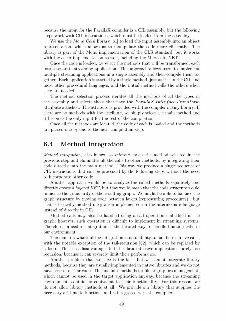
because the input for the ParallaX compiler is a CIL assembly, but the followingsteps work with CIL instructions, which must be loaded from the assembly.

We use the Mono Cecil library [81] to load the input assembly into an objectrepresentation, which allows us to manipulate the code more efficiently. Thelibrary is part of the Mono implementation of the CLR standard, but it workswith the other implementation as well, including the Microsoft .NET.

Once the code is loaded, we select the methods that will be transformed, eachinto a separate streaming application. This approach allows users to implementmultiple streaming applications in a single assembly and then compile them to-gether. Each application is started by a single method, just as it is in the CIL andmost other procedural languages, and the initial method calls the others whenthey are needed.

The method selection process iterates all the methods of all the types inthe assembly and selects those that have the ParallaX.Interface.Transformattribute attached. The attribute is provided with the compiler in tiny library. Ifthere are no methods with the attribute, we simply select the main method andit becomes the only input for the rest of the compilation.

Once all the methods are located, the code of each is loaded and the methodsare passed one-by-one to the next compilation step.

6.4 Method Integration

Method integration, also known as inlining , takes the method selected in theprevious step and eliminates all the calls to other methods, by integrating theircode directly into the main method. This way we produce a single sequence ofCIL instructions that can be processed by the following steps without the needto incorporate other code.

Another approach would be to analyze the called methods separately anddirectly create a layered HFG, but that would mean that the code structure wouldinfluence the granularity of the resulting graph. We might be able to balance thegraph structure by moving code between layers (representing procedures) , butthat is basically method integration implemented on the intermediate languageinstead of directly in CIL.

Method calls may also be handled using a call operation embedded in thegraph; however, such operation is difficult to implement in streaming systems.Therefore, procedure integration is the favored way to handle function calls inour environment.

The main drawback of the integration is its inability to handle recursive calls,with the notable exception of the tail-recursion [82], which can be replaced bya loop. This is a disadvantage, but the data intensive applications rarely userecursion, because it can severely limit their performance.

Another problem that we face is the fact that we cannot integrate librarymethods, because they are usually implemented in native libraries and we do nothave access to their code. This includes methods for file or graphics management,which cannot be used in the target application anyway, because the streamingenvironments contain no equivalent to their functionality. For this reason, wedo not allow library methods at all. We provide our library that supplies thenecessary arithmetic functions and is integrated with the compiler.

49

Calling

method

Copy

code

Called

method

Integrated

method

Patameter

patch

Variable

renaming

Jump

extensionPatched calling

method

Patched called

method

Code

integration

Figure 6.2: Method integration process

We have implemented an explicit method integration algorithm, because wehave to eliminate method calls in the analyzed code. The CLR just-in-timecompiler , or JIT for short, integrates small methods, when the code is loaded forexecution, which is too late for us. We needed to be able to integrate methodsin the CIL so we can produce a code without any calls and transform it to HFG.The following sections describe the process in detail.

6.4.1 Integration overview

The integration process is straightforward but requires many technical detailsto be addressed for the code to be valid according to the standard [30]. Theintegration always integrates a single called method into a calling method . Ifa method calls multiple methods then they are integrated one after another.Figure 6.2 show the entire integration process for a single method. We use theCecil library, which allows us to change the code efficiently without complexbinary calculations.

The first step is to copy the code of the called method, because we do not wantto modify the original code, because that would make it invalid. On the otherhand, we can modify the calling method, because it will be fully valid at the endof the integration. The further steps are described in the following sections indetail.

6.4.2 Variable Renaming

We must rename all the local variables of the called method so that they do notconflict with variables of the calling method. This requires that we also patchthe instructions accessing the variables by swapping the original name for thenew one. Algorithm 2 shows the renaming, where the AvailableName methodgenerates a new variable name available in the calling method. For example:V ariableN : N ∈ N ∧ V ariableN /∈ V ar(calling).

6.4.3 Parameter Patch

Parameters of the called method must be renamed as well, but they also have to bereplaced by local variables and the instructions accessing them changed to reflectthis. The process is the same as for the local variables, with the exception, thatwe also change the instruction operation code. Store argument (starg) is changedto store local (stloc) instruction and load argument (ldarg) is changed to loadlocal (ldloc) instruction. The actual implementation is a bit more complicated,

50

Algorithm 2 Variable renaming

Require: I – instructions of the called methodV – local variables of the called methodC – local variables of the calling method

Ensure: M – patched called method{Rename variables}

1: REG := ∅ // associative register mapping renamed and original variables2: for all v ∈ V do3: rv := AvailableName(v, C)4: C := C ∪ {rv}5: REG := REG ∪ {(v, rv)}6: end for{Patch instructions}

7: for all i ∈ I do8: if i.Operand ∈ V then9: i.Operand := REG[i.Operand]10: end if11: end for12: M := (C, I)

because it has to properly transform all the specific versions of the instructionto their appropriate counterparts, for example the transformation must preservethe difference between integer and object versions of the instructions or the codewould be invalid.

6.4.4 Jump Extension

Before we integrate the code, we have to first ensure that all the jumps in thecalling method will remain valid. This means that we have to locate all the jumpsthat traverse the integrated call instructions and extend them by the number ofinstructions in the called method. Algorithm 3 shows the entire process, we assumethat the instructions can be compared according to their position in the code.Jump instructions contain target offset (relative distance) as their operand.

6.4.5 Code Integration

The code can be copied to the calling method, once both the methods are pre-pared. The call instruction is replaced by all the previously copied and patchedinstructions of the called method.

6.4.6 Stack Limit

There is one last technical detail that has to be addressed for the code to bevalid. The .NET runtime require all methods to indicate the maximal size of thestack they require, see Section 3.3 for details. This information has to be updatedfor the calling method, because the integrated code can change the require size.We calculate the new size by adding the required size of the calling and calledmethods:

51

Algorithm 3 Jump extension

Require: I – instructions of the calling methodC ∈ I – the call instructionJUMP – list of all jump instruction codesN – number of instructions of the called method

Ensure: M – patched instructions1: for all i ∈ I do2: if i.OpCode ∈ JUMP then3: if i < C ∧ i+ i.Operand > C then4: i.Operand := i.Operand+N5: else if i > C ∧ i+ i.Operand < C then6: i.Operand := i.Operand−N7: end if8: end if9: end for10: M := I

calling.MaxSize := calling.MaxSize+ called.MaxSize (6.1)

6.5 Code Preprocessing

Before we transform the CIL code to the hybrid flow graph, we have to prepare itfor the compiler. The preprocessor accepts a single sequence of CIL instructionswithout calls, produced by the method integration, and produces another sequencewithout calls.

The inherent structure of a procedural code has one important feature thathas to be addressed, before it can be transformed to a Hybrid flow graph. Themost important fact is that procedural application has a memory that is set oncebut can be read multiple times. This is not possible in streaming environments,because that would mean that such ”variable” would have to be connected toall kernels that access its value, which would limit the available parallelism andcause unnecessary synchronization.

There are two situations, where the lack of persistent storage can cause prob-lems. The code in Listing 6.2 shows a situation, where the variable x is repeatedlyread in a loop without being assigned there and we have to repeatedly reproducethe value in the resulting graph. The second situation is in Listing 6.3, where thevariable y is updated in every other iteration of a loop and we have to preservethe correct value through all the iterations.

Listing 6.2: Value recyclation

int x = 2 ;int y = 0 ;for ( int i = 0 ; i < 5 ; i++){

y = y + x ;}

52

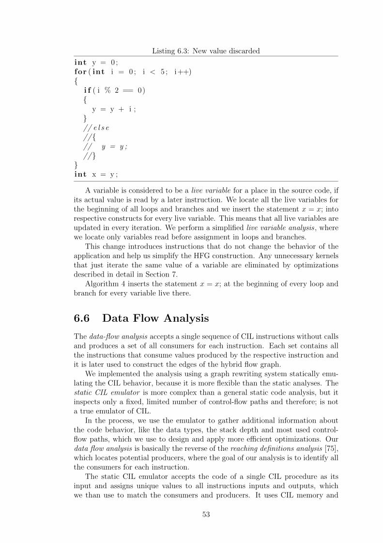
Listing 6.3: New value discarded

int y = 0 ;for ( int i = 0 ; i < 5 ; i++){

i f ( i % 2 == 0){

y = y + i ;}// e l s e//{// y = y ;//}

}int x = y ;

A variable is considered to be a live variable for a place in the source code, ifits actual value is read by a later instruction. We locate all the live variables forthe beginning of all loops and branches and we insert the statement x = x; intorespective constructs for every live variable. This means that all live variables areupdated in every iteration. We perform a simplified live variable analysis , wherewe locate only variables read before assignment in loops and branches.

This change introduces instructions that do not change the behavior of theapplication and help us simplify the HFG construction. Any unnecessary kernelsthat just iterate the same value of a variable are eliminated by optimizationsdescribed in detail in Section 7.

Algorithm 4 inserts the statement x = x; at the beginning of every loop andbranch for every variable live there.

6.6 Data Flow Analysis

The data-flow analysis accepts a single sequence of CIL instructions without callsand produces a set of all consumers for each instruction. Each set contains allthe instructions that consume values produced by the respective instruction andit is later used to construct the edges of the hybrid flow graph.

We implemented the analysis using a graph rewriting system statically emu-lating the CIL behavior, because it is more flexible than the static analyses. Thestatic CIL emulator is more complex than a general static code analysis, but itinspects only a fixed, limited number of control-flow paths and therefore; is nota true emulator of CIL.

In the process, we use the emulator to gather additional information aboutthe code behavior, like the data types, the stack depth and most used control-flow paths, which we use to design and apply more efficient optimizations. Ourdata flow analysis is basically the reverse of the reaching definitions analysis [75],which locates potential producers, where the goal of our analysis is to identify allthe consumers for each instruction.

The static CIL emulator accepts the code of a single CIL procedure as itsinput and assigns unique values to all instructions inputs and outputs, whichwe than use to match the consumers and producers. It uses CIL memory and

53

Algorithm 4 CIL code variable access patch

Require: I – sequence of instructionsL – sequence of all loops ∀l ∈ L : l ⊆ I

Ensure: C – patched set of instructions1: C := I2: for all l ∈ L do3: V := ∅4: P := ∅5: for all i ∈ l do6: if i == ldl then7: V := V ∪ {i.Operand}8: end if9: if i == ldarg then10: P := P ∪ {i.Operand}11: end if12: end for13: for all v ∈ V do14: C = C[0 : l.start]|[ldl v]|[stl v]|C[l.start : C.length]15: end for16: for all p ∈ P do17: C = C[0 : l.start]|[ldarg p]|[starg p]|C[l.start : C.length]18: end for19: end for

execution model (variables, stack and program counter) transformed to a graph.This emulator is not a hybrid flow graph, even though it uses graph rewriting todefine its semantics. The emulator uses CIL instruction behavior specified in theECMA standard [30] to properly model the CIL behavior.

Instead of emulating the actual calculation, we modify the instruction behav-ior, the instructions then exchange unique identifiers instead of actual values andwe store all the identifiers consumed and produced for each instruction. Thisway, we assign a unique identifier to each input and output and we can producethe consumer sets that are the final output of the data-flow analysis. We emulateonly the minimal number of control-flow paths to limit the complexity of theanalysis. The initialization and emulation is explained in the next sections.

Listing 6.4 shows identifiers assigned by our emulator to the CIL instructionsof the factorial method (original C# code is in Listing 4.1), where the identifiersare shown as (inputs)→ (outputs).

We take the identified values and produce the sets of consumers according otthe Algorithm 5, which iterates over all the instructions and assigns each the setof consumers based on the values the instruction produces. The final result ofthe entire data-flow analysis for the factorial method is in Listing 6.5.

6.6.1 CIL Sequential Graph

A CIL sequential graph is an annotated directed graph, with semantics definedby a graph rewriting system. It has a strict control flow that directly copiesthat of the source code using a program counter and it has nodes representing

54

IL 0000 : ldc . i 4 . 1 ()−>( id1 )IL 0001 : s t l o c . 0 ( id1)−>( id2 )// loop s t a r t ( head : IL 0002 )IL 0002 : lda rg . 0 ( p1 , id10)−>( id3 )IL 0003 : l d l o c . 0 ( id2 , id6)−>( id4 )IL 0004 : mul ( id3 , id4)−>( id5 )IL 0005 : s t l o c . 0 ( id5)−>( id6 )IL 0006 : lda rg . 0 ( p1 , id10)−>( id7 )IL 0007 : ldc . i 4 . 1 ()−>( id8 )IL 0008 : sub ( id7 , id8)−>( id9 )IL 0009 : s t a r g . s a ( id9)−>( id10 )IL 000b : lda rg . 0 ( id10)−>( id11 )IL 000c : ldc . i 4 . 1 ()−>( id12 )IL 000d : bgt . s IL 0002 ( id11 , id12 )−>()// end loopIL 000 f : l d l o c . 0 ( id6)−>( id13 )IL 0010 : r e t ( id13 )−>()

Listing 6.4: Produced and consumed values

IL 0000 : ldc . i 4 . 1 { IL 0001}IL 0001 : s t l o c . 0 { IL 0003}// loop s t a r t ( head : IL 0002 )IL 0002 : lda rg . 0 { IL 0004}IL 0003 : l d l o c . 0 { IL 0004}IL 0004 : mul { IL 0005}IL 0005 : s t l o c . 0 { IL 0003 , IL 000 f }IL 0006 : lda rg . 0 { IL 0008}IL 0007 : ldc . i 4 . 1 { IL 0008}IL 0008 : sub { IL 0009}IL 0009 : s t a r g . s a { IL 0002 , IL 0006 , IL 000b}IL 000b : lda rg . 0 { IL 000d}IL 000c : ldc . i 4 . 1 { IL 000d}IL 000d : bgt . s IL 0002 {}// end loopIL 000 f : l d l o c . 0 { IL 0010}IL 0010 : r e t {}

Listing 6.5: Data-flow analysis assigned consumer sets

55

Algorithm 5 Consumer set construction

Require: I – sequence of instructionsIN – array containing sets of all the values consumed by each instructionOUT – array containing sets of all the values produced by each instruction

Ensure: C – array containing sets of consumers for every instruction1: for all i ∈ I do2: C[i] := ∅3: for all j ∈ I do4: if OUT [i] ∩ IN [j] then5: C[i] := C[i] ∪ {j}6: end if7: end for8: end for

all variables, arguments and one for the stack, see Section 3.3 for details of theCIL language. Figure 6.3 shows a sample CIL sequential graph representing thefactorial method, where the nodes annotated in upper case represent the specialoperations implementing the execution stack (STACK), the variable a (V AR),the argument p (ARG) and the program counter (P ). The variables have aninitial value according to the CIL standard and the stack has an empty value sowe do not have to define separate semantics for an empty stack.

ARG

STACK

P ldc

VAR

stloc ldarg ldloc mul stloc ldarg

ldc

substargldargldcbgtldlocret

0 0

head

Figure 6.3: CIL sequential graph representing the factorial method

The CIL sequential graph is a parallel to the hybrid flow graph, but it isnot the same because it has a completely different semantics and its structure isuseless for streaming environments as it provides only a very limited parallelism.

The semantics of the CIL sequential graph are defined using a graph rewritingsystem based on the CIL semantics defined in its standard [30]. Figure 6.4 con-tains the rules defining the behavior of the basic CIL instructions, we present onlythe rules necessary for our examples, the rest are defined the same way accordingto the behavior of the respective instructions. It is important to note that theedges graphical design defines its annotation, which is most important for theconditional jumps, where the thicker dashed edge represents the jump and theregular edge is used when the condition is false.

The semantics directly copy the CIL standard, mainly the stack management.

56

ldc x STACKP ldc x STACK

P x

mul STACKP mul STACK

P x*y

y

x

ldloc x STACKP ldloc x STACK

P x

VAR a VAR axx

stloc x STACKP stloc x STACK

Px

VAR a VAR axy

bgt STACKP bgt STACK

P

x

bgt STACKP bgt STACK

Py

x > y x < y

x

y

Figure 6.4: Semantics of selected CIL sequential HFG operations

The control-flow is driven by the program counter (node P ), which follows theedges between instructions. The data management is handled by the stack andvariable operations, where each instruction consumes and produces the propernumber of stack levels or changes the variable values, based on its definition. Theconstruction of the CIL sequential graph is described later in Section 6.6.4.

The CIL sequential graph execution follows the same principle as a graphrewriting system, rules are applied as long as there is at least one applicable. Theexecution copies the work of the CLR virtual machine, the control flow followsthe same path, variables and stack contain the same value after every evaluatedinstruction and there is always at most one applicable rule, because there is onlyone program counter (P ).

6.6.2 Symbolic Semantics of the CIL Sequential Graph

To analyze the data flow, we must introduce a modified version of the CIL sequen-tial graph. The symbolic semantics do not emulate the CIL calculation, insteadwe collects the consumed values.

We define the symbolic semantics of the CIL sequential graph by anothergraph rewriting system. The modified rules work with instruction identifiersinstead of actual values. This way, we can analyze which instructions consumethe values produced other instructions. The example symbolic rules are shownin Figure 6.5, we modify other rules the same way.

We assign each instruction an identifier equal to its position in the sequence

57

ldloc x STACKP ldloc x STACK

P ID

VAR a VAR aID1ID1

bgt STACKP bgt STACK

P

ID1

ID ID

ID1

X X-1

ID2

Figure 6.5: Symbolic semantics of selected Sequential HFG operations

(∀i ∈ I : id(i) = i). Last modification is that the rules store identifiers ofconsumed values, this is indicated by the bold dash-edged nodes in Figure 6.5.

The identifiers of branches decide how many times the branch is evaluatedas true and how many times it is false, we use this to drive the control flow(explained in the next section). Branches do not require an identifier, becausehey do not produce any values, they just change the execution order.

6.6.3 Execution of the Symbolic CIL Sequential Graph

We use the symbolic semantics defined in the previous section to analyze thevalues produced and consumed by instructions, we call this process a symbolicCIL emulation. The symbolic semantics work with instruction identifiers insteadof actual values and conditional branches behavior is predefined. The result ofthe symbolic emulation is a list of consumed values we than use to construct setsof consumers for each instruction.

The symbolic emulation requires one extra step before the standard rule ap-plication. The conditional branches have to be setup with information about theway they should be executed. This means simply assigning a number to eachbranch defining how many times it is evaluated as true and false. To cover allthe possible execution paths, we have to use all combinations of branches – eachjump must be at least twice true and false for every other nested jump, whichleads to the maximum of 4#jumps execution paths. This is necessary to modelthe loops, where the first iteration consumes values produced before the loop andall the following iterations consume the values produced by the loop itself. Thenumber of passes may be high, but the emulator is very efficient, because it usesonly the instruction stack behavior, which is a constant number, to model thedata-flow. This process is not valid for loops with goto and break, but we do notallow these constructions in the input code, Section 5.3 contains details.

Algorithm 6 defines the symbolic CIL emulation process. I is a set of arraysthat define the setup information for each node (a positive number) – the numberof true and false evaluations for jumps and identifiers for the other instructions.The applicable and apply functions check and apply the symbolic rules, theyimplement the graph rewriting system functionality. The extract ids functionobtains the values consumed by the node (dashed boxes in Figure 6.5).

The conditional jumps are evaluated based on their identifier x according tothe formula x ≥ 0, which means that the emulator jumps while the identifier ispositive. This way we change the number of loop iterations, because the loop

58

Algorithm 6 Symbolic emulation

Require: G – CIL sequential graphR – symbolic rulesI – list of setup information

Ensure: ID – list of collected IDs1: for all i ∈ I do2: Gs := G3: for all v ∈ V (G) do4: V (Gs) := V (Gs) ∪ {i[v]}5: E(Gs) := E(Gs) ∪ {(i[v], v)}6: end for7: while ∃r ∈ R : applicable(Gs, r) do8: Gs := apply(Gs, r)9: end while10: ID := ∅11: for all v ∈ V (G) do12: ID[v] := (v, extract ids(v), i[v]);13: end for14: end for

ends once the jumps identifier is x < 0.

Result of the algorithm is an aray of sets of consumed and produced valuesfor each node / instruction in the CIL sequential graph. The array is constructedusing the function extract ids that extracts the identifiers of the nodes / instruc-tions. The lists are used to construct the consumer sets that are the output ofthe entire data-flow analysis.

6.6.4 Construction of the CIL Sequential Graph

The construction of the CIL sequential graph is straightforward and requires onlythe code sequence and static information about instructions, we do not need anyadditional analyses. The basic transformation of a CIL code to a CIL sequentialgraph requires the following four steps:

59

1. Create nodes based on the instructions.

2. Connect the instruction nodes based on the control-flow sequence.

• Standard instructions follow one another.

• Conditional jumps have two outgoing edges, one to the jump target(specified by its operand) and the other leading to the next instruction.

• Fixed jumps have only one edge going to the jump target.

3. Create special nodes for stack, program counter, variables and arguments.

4. Connect the instruction nodes to the special nodes based on their data-flowbehavior.

• Program counter node is connected to the first instruction in the code.

• All instructions are connected to the stack.

• Instructions that access a variable (based on their operand) are con-nected to its node.

The entire transformation is in Algorithm 7. The instruction set I and variableset M are extracted from the source code and the sets J and F contain instructioncodes of all conditional and fixed jumps respectively, as defined in CIL standard[30]. Each instruction contains information about its code and operand accessedusing the comma operator. The transformation can be illustrated on the exampleof the factorial method, Listing 6.4 contains the CIL source code and Figure 6.3shows the resulting graph.

6.6.5 Instruction Classifier

The instruction classifier accepts a single sequence of CIL instructions as itsinput and it produces a sequence of classification tokens. A classification tokenis a tiny structure that contains a classification and the respective instruction, ifrelevant. The classification defines the instruction type and it is a value from thefollowing list:

• INSTRUCTION – Basic instruction that does not change control-flow.

• FIXED – Instruction representing a fixed (non-conditional) jump.

• CONDITIONAL – Instruction representing a conditional jump.

• TARGET – Target place of a single jump. The token is not associatedwith an instruction, because it represents a space between instructions.

We processes the code one instruction at a time and using a table we assigneach instruction a classification token. We create a sequence of the classificationtokens representing the instructions, classified as either the INSTRUCTION ,FIXED or CONDITIONAL. Then we locate all the jumps and for each jump,we add a token with the TARGET classification just before the instruction that

60

Algorithm 7 Transformation of CIL to Sequential HFG

Require: I – sequence of instructions (source code)M – set containing all variables and argumentsJ – conditional jump instruction codesF – fixed jump instruction codes

Ensure: G – CIL sequence graph{Special nodes}

1: V := {P, STACK} ∪ {Vm : m ∈M}{Instruction nodes}

2: V := V ∪ {Vi : i ∈ I}{Control-flow edges}

3: E := {(P, V0∈I)}4: for all i ∈ I do5: if i.code ∈ J then6: E := E ∪ {(Vi, Vi.operand∈I)}7: E := E ∪ {(Vi, Vi+1)}8: else if i.code ∈ F then9: E := E ∪ {(Vi, Vi.operand∈I)}10: else11: E := E ∪ {(Vi, Vi+1)}12: end if13: end for{Data-flow edges}

14: for all i ∈ I do15: if i.code ∈ {stloc, ldloc, starg, ldarg} then16: E := E ∪ {(Vi, Vi.operand∈M)}17: end if18: end for19: G := (V,E)

61

Listing 6.6: Lexer tokens

IL 0000 : ldc . i 4 . 1 (INSTRUCTION, ldc )IL 0001 : s t l o c . 0 (INSTRUCTION, s t l o c )// loop s t a r t ( head : IL 0002 ) (TARGET, n u l l )IL 0002 : lda rg . 0 (INSTRUCTION, ldarg )IL 0003 : l d l o c . 0 (INSTRUCTION, l d l o c )IL 0004 : mul (INSTRUCTION, mul )IL 0005 : s t l o c . 0 (INSTRUCTION, s t l o c )IL 0006 : lda rg . 0 (INSTRUCTION, ldarg )IL 0007 : ldc . i 4 . 1 (INSTRUCTION, ldc )IL 0008 : sub (INSTRUCTION, sub )IL 0009 : s t a r g . s a (INSTRUCTION, s t a rg )IL 000b : lda rg . 0 (INSTRUCTION, ldarg )IL 000c : ldc . i 4 . 1 (INSTRUCTION, ldc )IL 000d : bgt . s IL 0002 (CONDITIONAL, bgt )// end loopIL 000 f : l d l o c . 0 (INSTRUCTION, l d l o c )IL 0010 : r e t (FIXED, r e t )

is the operand of the jump (its target).Listing 6.6 shows the classification tokens for the factorial method defined in

Listing 4.1. The token TARGET is not assigned to an instruction, it is placedbetween instructions because it represents the target of a jump.

6.7 Control Flow Analysis

In this section, we will explain in detail the final step of the front-end of theParallaX compiler – the control-flow analysis. We start by analyzing the availablecontrol flow constructs and their representation in a hybrid flow graph. Then weexplain the algorithms used to transform the procedural code to a hybrid flowgraph, based on the control-flow structure.

The control-flow analysis consumes the output of both the instruction clas-sifier and data-flow analysis and produces a hybrid flow graph, the graph isgradually expanded as the code is analyzed. We parse the code, one instructionat a time, and we either add the new instruction directly to the graph (in caseof basic instructions), or we create a control flow sub-graph and connect it tothe main graph. Basic instructions do not influence the control-flow, they aredirectly transformed into an appropriate node and then connected according todata flow. Control flow constructs are handled in three steps:

1. Recursively create the sub-graph representing the loop or branch body.

2. Add special operations that handle the data flow.

3. Connect the created graph into the final HFG according to the data-flow.

One special construct is the HFG start node. It is used to start the entire

62

graph and it does not have any input from inside of the graph. It sends an inputto nodes that do would not have an input otherwise, like a load constant. Thestarting impulse must be specially handled in control flow, because in branch-es only some operations must be started (in active branch) and some must berestarted (in loops).

6.7.1 Branch Infrastructure

Each conditional branch, also known as if-else, is composed of a condition andtwo branches (represented by sub-graphs), which can be empty. The basic infras-tructure used to represent a branch is shown in Figure 6.6 (left), it is the onlyinterface between the branches and the rest of the HFG.

S

1

2

x cond

M

1 2

BBtrue

3

BBfalse

xnew

previous BB

branch

body

next BB

post-branch

infrastructure

pre-branch

infrastructure M

1 3

x

cond

S1

body

2

xnew

previous BB

loop

body

next BB

loop output

infrastructure

loop input

infrastructure 2

L

start

Figure 6.6: Branch (left) and loop (right) infrastructure

Figure 6.6 shows the branch with the surrounding code, where the previousbasic block and both branches are already constructed and the next basic blockis connected once it is ready. The infrastructure is built around the branches andit serves as their only interface with the rest of the HFG. The figure defines theinfrastructure for a single variable. The special nodes (pre-branch and post-branchsections) must be replicated for each variable used in the branch.

For branches we use combination split-merge, where the split separates datafor branches and merge collects them at the end. Split-merge interface is createdonly for values used in the branch (accessed variables or arguments). The splitand merge nodes are defined in Section 4.3 as part of the Hybrid Flow Graphsemantics.

The infrastructure must make sure that the right branch is executed, based onthe condition. And it must ensure that only one branch is executed at a time, nonodes from the other can executed, because that would mean that unused valuesmay remain in the graph and make further computations skewed or completelyinvalid.

The starter node is handled like a variable, by a split-merge, and it is addedonly if a starter impulse is necessary (when a branch contains a node withoutinput, like a load constant).

If one of the branches does not modify a variable, we simply connect the splitto the merge, thus the value is transfered unchanged. When a variable is not

63

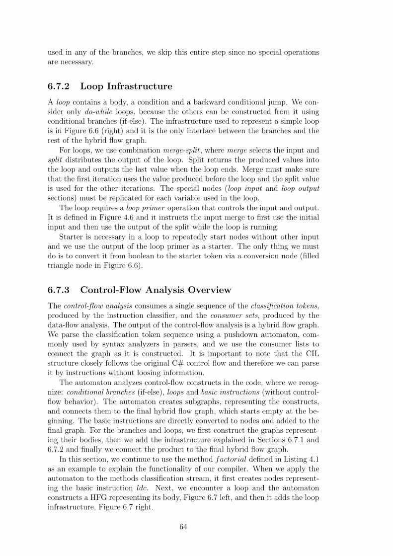
used in any of the branches, we skip this entire step since no special operationsare necessary.

6.7.2 Loop Infrastructure

A loop contains a body, a condition and a backward conditional jump. We con-sider only do-while loops, because the others can be constructed from it usingconditional branches (if-else). The infrastructure used to represent a simple loopis in Figure 6.6 (right) and it is the only interface between the branches and therest of the hybrid flow graph.

For loops, we use combination merge-split , where merge selects the input andsplit distributes the output of the loop. Split returns the produced values intothe loop and outputs the last value when the loop ends. Merge must make surethat the first iteration uses the value produced before the loop and the split valueis used for the other iterations. The special nodes (loop input and loop outputsections) must be replicated for each variable used in the loop.

The loop requires a loop primer operation that controls the input and output.It is defined in Figure 4.6 and it instructs the input merge to first use the initialinput and then use the output of the split while the loop is running.

Starter is necessary in a loop to repeatedly start nodes without other inputand we use the output of the loop primer as a starter. The only thing we mustdo is to convert it from boolean to the starter token via a conversion node (filledtriangle node in Figure 6.6).

6.7.3 Control-Flow Analysis Overview

The control-flow analysis consumes a single sequence of the classification tokens,produced by the instruction classifier, and the consumer sets, produced by thedata-flow analysis. The output of the control-flow analysis is a hybrid flow graph.We parse the classification token sequence using a pushdown automaton, com-monly used by syntax analyzers in parsers, and we use the consumer lists toconnect the graph as it is constructed. It is important to note that the CILstructure closely follows the original C# control flow and therefore we can parseit by instructions without loosing information.

The automaton analyzes control-flow constructs in the code, where we recog-nize: conditional branches (if-else), loops and basic instructions (without control-flow behavior). The automaton creates subgraphs, representing the constructs,and connects them to the final hybrid flow graph, which starts empty at the be-ginning. The basic instructions are directly converted to nodes and added to thefinal graph. For the branches and loops, we first construct the graphs represent-ing their bodies, then we add the infrastructure explained in Sections 6.7.1 and6.7.2 and finally we connect the product to the final hybrid flow graph.

In this section, we continue to use the method factorial defined in Listing 4.1as an example to explain the functionality of our compiler. When we apply theautomaton to the methods classification stream, it first creates nodes represent-ing the basic instruction ldc. Next, we encounter a loop and the automatonconstructs a HFG representing its body, Figure 6.7 left, and then it adds the loopinfrastructure, Figure 6.7 right.

64

bgt

ldc 1 sub

1

2

12

mul2

M L

S

3

1

2

1

2

1

2

bgt

ldc 1sub

1

2

1 2

M

S

3

1

2

1

2

mul

1

2

Figure 6.7: factorial loop body (left) and infrastructure (right).

Finally, we connect the loop to the ldc node and complete the graph by addingthe return ret node. We eliminate instructions like load local (ldloc), because theydo not modify data, they are removed by the optimizations presented in the nextchapter. The complete graph is in Figure 6.8.

M L

S

3

1

2

1

2

1 2

bgt

ldc 1sub

1

2

1 2

M

S

3

1

2

1

2

ldc 1

ret

mul

1

2

Pa I

R

Figure 6.8: The HFG representation of the factorial function

6.7.4 Hybrid Flow Graph Construction

To analyze the control flow, we designed a pushdown automaton based on acontext-free grammar. The grammar takes the classifications , produced by the in-struction classifier, as terminals and assigns semantic values to the non-terminalslike a purely-synthesized attribute grammar. The automaton is generated fromthe grammar in Listing 6.7, where the used functions are explained in the follow-ing text. The functions are defined using pseudo-code algorithms, which containthe implementation without technical details that would make them too long.

For basic instruction, the AddBasicNode function creates a small graph con-taining a node representing the instruction and its input nodes connected byedges. The function is defined in Algorithm 9. The block rule then connectsthe new graph with the main HFG using the MergeGraph function defined inAlgorithm 9.

65

Listing 6.7: Parser grammar

s t a r t :b lock{ $$ = CompleteGraph ( $1 ) ; }

;b lock :

b lock cons t ruc t{ $$ = MergeGraph ( $1 , $2 ) ; }| cons t ruc t{ $$ = $1 ; }

;c on s t ruc t :

i n s t r u c t i o n{ $$ = $1 ; }| i f{ $$ = $2 ; }| loop{ $$ = $2 ; }

;i n s t r u c t i o n :

INSTRUCTION{ $$ = AddBasicNode ( $1 ) ; }

;i f :

CONDITIONAL block FIXED TARGET block TARGET{ $$ = AddBranch ( $1 , $2 , $5 ) ; }| CONDITIONAL block TARGET{ $$ = AddBranch ( $1 , $2 , EmptyGraph ) ; }

;loop :

TARGET block CONDITIONAL{ $$ = AddLoop( $4 , $2 ) ; }

;

Algorithm 8 AddBasicNode

Require: REG – associative register mapping instructions to nodesI – CIL instructionIN – the number of inputs of I

Ensure: G – graph representing iREG′ – updated register

1: N := {VI} ∪ {In : n ∈ Z ∧ n ≥ 0 ∧ n < IN}2: E := {(In, VI) : In ∈ N} ∪ {([I], In) : In ∈ N}3: REG[I] := VI4: G = (N,E)5: REG′ = REG

66

The graphs are created with input edges that do not have source, but they areannotated with the identifier of the value they represent, [I] in the algorithms.These empty edges are connected according to the consumer sets when the sub-graph is merged to the HFG. We start HFG creation with the first instruction,which has no inputs because the stack is empty, and then we merge others to it.During the construction, we continually update a register mapping the construct-ed nodes to the original instructions so we can properly connect them accordingto the data-flow analysis.

Algorithm 9 MergeGraph

Require: REG – associative register mapping instructions to nodesSET – consumer sets, produced by data-flow analysisG – previous version of HFGS – subgraph

Ensure: HFG – new HFG1: HFG := (G.N ∪ S.N,G.E ∪ S.E)2: Empty := ((I, V ) ∈ HFG.E : I /∈ HFG.V )3: HFG.E = HFG.E \ Empty4: for all (I, V ) ∈ Empty do5: HFG.E = HFG.E ∪ {(REG[SET [I]], V )}6: end for

The function AddBranch, used in the rules for conditional branches (if-then-else and if-then), creates a subgraph consisting of the conditional jump instruc-tion, and either one or two branches. The jump instruction itself is converted asa basic instruction, because it contains the condition (e.g. bgt – branch if greaterthan). Then we create the split-merge infrastructure, explained in Section 6.7.1,and we connect the branch inputs to the splits and the outputs to the merges.The resulting graph is then merged to the final HFG using the MergeGraphfunction.

The AccessedV ariables function collects all the variables and arguments ac-cessed by at least one node in a graph. The accessed variables are then usedto construct the split-merge infrastructure for the conditional branch, which ishandled by the AddSplitMerge function. The merge-split infrastructure replacesthe variables in the register (REG) with the appropriate merge or split output.

The rule for do-while loops is similar to that for the conditionals, but it usesthe loop infrastructure described in Section 6.7.2.

The rule for the complete graph connects the HFG after all instructions andcontrol flow constructs are processed. The function CompleteGraph adds a globalstarter node (I), parameter nodes (P x) and a return node (R). We add thesenodes here because it is the root non-terminal that has to produce a completehybrid flow graph.

6.7.5 Broadcast Introduction

One last step is necessary to make the final hybrid flow graph valid, we have tointroduce broadcast operations, which ensure that every other operation exceptsplit has just a single output. The process is defined in Algorithm 12, where abroadcast is introduced for every node with more than one output.

67

Algorithm 10 AddBranch

Require: REG – associative register mapping instructions to nodesSET – consumer sets, produced by data-flow analysisJ – conditional jumpB0 – false branchB1 – true branch

Ensure: G – new HFG1: G := AddBasicNode(REG, J)2: V alues := AccessedV ariables(REG,G1, G2)3: for all val ∈ V alues do4: G := MergeGraph(REG,SET,G,AddSplitMerge(REG, val))5: end for6: G := MergeGraph(REG,SET,G,B0)7: G := MergeGraph(REG,SET,G,B1)

Algorithm 11 AddLoop

Require: REG – associative register mapping instructions to nodesSET – consumer sets, produced by data-flow analysisJ – conditional jumpB – loop body

Ensure: G – new HFG1: G := AddBasicNode(REG, J)2: V alues := AccessedV ariables(Body)3: for all val ∈ V alues do4: G := MergeGraph(REG,SET,G,AddMergeSplit(REG, val))5: end for6: G := AddLoopPrimer(REG,G)7: G := MergeGraph(REG,SET,G,B)

Algorithm 12 AddBroadcasts

Require: G – complete hybrid flow graphEnsure: H – modified HFG1: V := V (G)2: E := E(G)3: for all v ∈ V : v.code 6= split ∧ |{o ∈ V : {(v, o) ∈ E}}| > 1 do4: OUT := {o ∈ V : (v, o) ∈ E}5: E := E \ {(v, o) ∈ E : o ∈ OUT}6: V := V ∪ {b : b.code = broadcast}7: E := E ∪ {(v, b)} ∪ {(b, o) : o ∈ OUT}8: end for9: H := (V,E)

68

6.7.6 Source Code and HFG Equivalence

Finally, we present sketch of a proof that the HFG, produced by the presentedalgorithm, is equivalent to the source code.

To prove the equivalence, we must prove 1) that each instruction is executedin a HFG if and only if it would have been executed in the source code, 2) thateach HFG operation produces the same output (including the order of values) asits CIL counterpart and 3) each operation can be executed multiple times withoutinfluencing its behavior.

When we prove both, we can conclude that when a HFG is executed, the sameinstructions are executed, they get the same input and produce the same outputas they do in the source code. This means that the outputs are the same and noadditional side effects were introduced.

The second requirement is fulfilled by the fact that basic operations are definedexactly according to a CIL instructions. They produce the same output with thesame input in the same order - when triggered multiple times with different inputsit produces the same sequence of outputs as the original. The only special case isinstructions without input, like ldc (load constant). These operations have inputin HFG so they can be triggered by control flow and the first requirement makessure that they are executed exactly as they are in the source code.

The first requirement can be proven via induction over basic blocks. Basicblocks in a HFG are subgraphs containing only basic operations. The blocks areconnected by special operations and their interface is a set of live variables.

The operations in a basic block are executed only when they receive input.This means that all the operations are executed once they get all the valuesin the block interface, because each operations gets an input (either from theinterface or from another operation). The starter node is special, we consider it aseparate block executed automatically. This behavior is the same as CIL, whereall instruction in a block are executed once the block starts.

Next we consider the branch infrastructure (Figure 6.6) and the semantics ofthe split operation. The infrastructure contains split for every variable accessedin any branch and once the these splits get input, they pass the data to just oneof the branches. They always select the same branch as they have the same inputcondition. The selected branch is executed, while the other is not. This behavioris the same as in CIL.

Loop infrastructure (Figure 6.6) is controlled by a set of split operations placedat the end of the loop body. These splits either return the data to the loop orpass it to the next basic block, which controls when the loop ends (block thatgets the data is executed). Their behavior is controlled by the loop condition.The loop ends once the condition is false, just as in CIL.

The final step is inductive, we have proved that a basic block is executed onceit gets inputs and that the control flow infrastructure distributes inputs properly.Now we use induction over the control flow complexity: 1) single basic blockexecuted (via starter) 2) loop and branch distribute inputs and thus start thecorrect basic block (body/branch or the next one). Thus every basic operationis executed if and only if it is executed in the source code.

69

6.8 Data types

The Hybrid flow graph is strongly typed to prevent unpredictable or incorrectbehavior. The data types are assigned to edges, where each edge has a single typethat defines what data can be transfered over it. The information is passed tothe streaming environment plan that uses it to properly define the data streams.In HFG, we use the data types based on the types available in C# and we thenmap the types to the data types of the target platform, C++ types in case of theBobox system.

We extract the data types during the data flow analysis, see Section 6.6, wherewe identify both the consumer identifier and the incoming type. The data typesof all potential producers for a single instruction must be identical or implicitlyconvertible (like int to long) and the compilation fails if the types do not match.It is important to note that all the CIL instructions have a single output, withthe exception of the instruction dup that duplicates its input and all its outputshave the same type as its input.

The data-flow analysis extracts the output type for each instruction using thefollowing rules that assign data type to each instruction based on its operationcode and operand:

• constant – the type is defined by the instruction suffix (I4 for Int32 etc.)

• conversions – the type is defined by the suffix

• load / store variable – the type is identical to the type of the variable

• load / store argument – the type is identical to the type of the argument

• arithmetical operations – the type is identical to the type of the inputs

• conditional jumps – the output is always bool

• fixed jumps – no output, the jumps are never part of the HFG

Data types for edges connecting basic nodes (representing CIL instructions)are all gathered in the data flow analysis. Control flow introduces special nodesthat are not part of the original CIL and their data types are dependent on thebasic nodes they connect. We solve this situation in the control-flow analysis,where we assign the edges data types once the branch or loop infrastructure isconnected to all its inputs and outputs. When the infrastructure is connected, wepropagate the data type from inputs, which are typed by the data flow analysis,through the special operations to all the edges.

6.9 Array Support

The compiler supports one dimensional arrays, treating them as any other da-ta type. The compiler supports only one dimensional arrays to limit potentialaliasing of the embedded arrays, which is extremely difficult to trace. Most im-portantly, multi dimensional arrays can be represented in an one dimensionalarray by appending the embedded arrays one after another. The process is il-lustrated in Figure 6.9, where the elements can be accessed using the following

70

formula: array[y ∗ width + x]. Thanks to this limitation, the data flow analysisis able to track the arrays through their entire lifetime and eliminate aliasing.

A1

A2

A3

A4

A1 A2 A3 A4A

A

Figure 6.9: Array flattening.

Arrays are transported as other data types, an entire array is a single valuein the stream. The elements are extracted by kernels only when needed. Thisapproach is not very efficient, especially when the array is accessed sparsely, butit allows us to support the arrays in any control flow structure including multiplenested loops. Without this approach, it would be impossible to manage loopscontaining both scalars and arrays, since the array streams would be longer andit would not be possible to match the values and loop iterations. The efficiencyis addressed by optimizations that unpack the arrays in situations where it ispossible and they restructure the graph around them so that the expansion ismanaged properly, see Sections 7.

We do not support objects, because they cause similar problems as the multi-dimensional arrays, and they are not necessary to implement the data intensiveapplications or database procedures. The purpose of the compiler is not to executeany C# code in a streaming environment, but to allow programmers to implementstreaming applications using a restricted C#.

6.10 Aliasing

The compiler strongly restricts the input language to limit the effects of aliasing,where a single memory location can be accessed via multiple symbolic names(pointers or references). There are two possible causes in of aliasing in a C#code, multiple references can point to a single object or multiple array indicescan point to the same array in a multi-dimensional array. There are also pointersin unsafe C# code, but we do allow the unsafe code at all.

Value types, like numbers, cannot cause aliasing, because they cannot beaccessed via references of indices and we do not allow boxing1. We allow only asingle data type with reference semantics – single-dimensional arrays. However;we handle the arrays in a way that they cannot introduce aliasing, because wealways transport the entire array as a single value and our data analysis tracksthe array from its creation and through all the statements that can access it. Theprocess is explained in Section 6.9.

There is one situation, where aliasing can happen: the parameters of theentire application can be single-dimensional arrays and multiple parameters cancontain a reference of the same array. There is no way for our data analysis todecide if the parameters are aliased and we assume that they are never aliased.

1Boxing is a process that converts a value type into a reference type by wrapping it intoa simple object. The process is used to allow the use of value types in contexts that requirereference types, like some containers.

71

This assumption may cause us problems in general applications, but we focus onthe data intensive applications and database queries, which can be analyzed andwe can ensure that the parameters are not aliased.

72

7. Optimization

The previous chapter explained the front-end of the ParallaX compiler that pro-duces a hybrid flow graph from C# code compiler to CIL. The produced HFG canbe, thanks to its structure, almost directly executed using a streaming system.However, the HFG produced by the front-end does not offer much kernel paral-lelism as there is always at most one data element at each edge. In addition, thecommunication overhead in the streaming system would probably cost more thanthe sequential execution of the original code, since all instructions are represent-ed by separate nodes. Fortunately, there are several transformations which mayimprove the level of parallelism available as well as reduce the synchronizationoverhead.

All the optimizations are a special case of a process we call the componentextractions . The optimizations are implemented as rules of an associative graphrewriting system that modifies a layered hybrid flow graph, where the HFG pro-duced by the front-end can be considered a layered HFG with a single layer. Theproduced layered HFG contains custom operations implemented by a subgraphthat they replace, which means that they represent more complex nodes withoutcommunication overhead (we rely on the C++ compiler to place the variablesinto registers). For a detailed description of the layered hybrid flow graph, seeSection 4.5.

In streaming environments, the custom operations become components (seeFigure 5.2) implemented in a single kernel, avoiding the communication overhead.In addition some custom operations can allow other operations to be vectorized,by replacing control-flow constructs, mainly loops.

The optimization process used in the ParallaX compiler generally involvesgraph transformations, since our intermediate language, the Hybrid Flow Graph,is graph-based [5]. The optimizations we use can be divided in two main groups:general and HFG-specific optimizations [1]. The general optimizations fulfill asimilar function as those used in traditional compilers, despite being implementedas a graph rewriting system.

We demonstrate the optimization technique on a vectoradd function that addstwo vectors and stores the result in third vector. The source code is in Listing 7.1.We transform the source code to a HFG and use the presented optimizations toimprove the efficiency of the resulting graph, which is in Figure 7.1. The graphis gigantic and inefficient and we will gradually improve it as we introduce andapply the optimizations.

In unoptimized HFG, any array is treated similarly to a elementary datatype, it is passed around the graph, undergoing partial modifications by storeinstructions which change the array at the referenced positions. Although thisbehavior might be efficiently mimicked by the implementation if the underlyingstreaming system allows passing data by reference, this is certainly not as effectiveas required. Therefore, the optimizations described below try to recognize typicalpatterns in array handling and transform them into alternative representationswhich avoid passing the array as a whole. Consequently, the movement of thecomplete array is used only as a fall-back behavior when these optimizations fail,which is sometimes inevitable given the general undecidability associated with

73

Listing 7.1: Vector addition

int [ ] vectoradd ( int [ ] a , int [ ] b , int [ ] c ){

for ( int i = 0 ; i < c . Length ; i++){

c [ i ] = a [ i ] + b [ i ] ;}return c ;

}

M L

S

31

2

1

2

1 2

clt

ldc 1add

1 2

1 2

M

S

3

1

2

12

ret

I

R

ldc 1

Pc

length

M

S

1

2

1

2

Pa

M

S

1

2

1

2

Pb

ldelem ldelem

addstelem

33

Figure 7.1: Hybrid flow graph representing the vectoradd function

Turing-complete programming environments.The optimizations introduce the split between code and plan generation de-

scribed in the compiler overview, Chapter 5. The split is defined by the layers ofthe produced layered HFG, where the top layer represents the execution plan andthe layers representing the custom operations are transformed to kernels. Theirimplementation is defined by the subgraph they replace (the left hand side ofthe optimization rule, for example Figure 7.3). Both the plan and the separateoperations are provided to the streaming environment for execution.

7.1 Related Work – Transformations Improving

Parallelism

In the optimization stage, the compiler restructures the intermediate code pro-duced by the front-end to produce a more efficient and compact code, which canbe than transformed into an application. The goals of the transformations aresimilar to some phases known from traditional compilers: the optimizations focuson better memory management and simple code restructuring [57], vectorization[36] or general parallelization [72].

The Hybrid Flow Graph requires custom optimizations that modify its struc-ture, usually reducing granularity of the operations. The basic optimization usedin the compiler is the component extraction, which performs a single graph trans-formation, replacing a subgraph by another [1]. The general principle is thenused to implement all the other optimizations.

74

The general optimizations focus mainly on vectorization of the array oper-ations. We locate arrays that are read or modified in a loop following certainstructure and we replace the inefficient array management with more efficientcustom nodes, able to perform the computations using vector instruction. Thisprocess usually involves advanced numerical methods that study the ranges ofarray indices [36], but we avoid this by restricting the graph structure eligiblefor optimization. We require that the array is either read or modified (not both)and the index used is always the variable controlling of the loop plus a constant.This constraint does not currently allow for maximal vectorization, but it sup-ports the most common patterns, see Chapter 11 for experimental results. Theoptimizations will be gradually improved to include more complex code.

Compilers can contain even more advanced optimizations that significant-ly modify the structure of the intermediate code. These optimizations includetransformation, like loop skewing [36], where the loop iterations are restructureto provide more predictable behavior. Our optimizations always restructure theHFG, because they rely on graph rewriting, but the current implementation doesnot yet support transformation that would completely restructure the code. Onepotential example is the use of the parallelogram blocks to optimize the matrix-based dynamic algorithms (like Levenshtein distance) [2], which is our main casestudy. At the moment, we apply this transformation manually (at the input C#code), but it is theoretically possible to do so automatically, which is one area ofour future study.

The HFG specific optimizations focus on removing the special operations in-troduced by control-flow, because they usually prevent efficient vectorization andmay limit kernel parallelism. We apply these optimizations after the graph hasbeen vectorized, because we can eliminate the control-flow infrastructure onlyif the surrounding graph no longer needs the them. The actual process is verysimilar to the dead code elimination commonly used in compilers [57, 36, 84].

7.2 Component Extraction

The component extraction is an operation that transforms a layered hybrid flowgraph to another layered HFG. The transformation itself is implemented as a ruleof an associative graph rewriting system defined over layered hybrid flow graphs.The transformation combines multiple nodes into one complex node, reducingboth the kernel parallelism and communication overhead. It can greatly improvethroughput of the graph, but it can also limit parallelism, so it has to be usedcarefully. The concept is shown in Figure 7.2, where three arithmetic operationsare replaced by a custom operation with the same behavior.

sub

mul

add

custom

1

2ldloc

ldloc ldloc

ldloc

stloc stloc

Figure 7.2: Component extraction application

75

The optimization can be applied to any subgraph, but we limit the applicationmostly to the bodies of loops which represent the most computation-heavy part ofthe code. This way, we are able to create one custom node for the loop body andvectorize the entire loop, if its structure supports it. The rule for the example inFigure 7.2 is in Figure 7.3, where the custom1 operation is implemented by thesecond layer, represented by the graph in dashed box titled custom1. The cus-tom operation code is represented by the node $1 which represents the subgraphmatched by the [add|mul|sub|div]∗ node in the pattern graph.

[add|mul|

sub|div]*

stloc

ldloc ldloc

1 2

1

custom1

stloc

ldloc ldloc

1 2

1

$1

1 2

custom1

Figure 7.3: Component extraction pattern graph

The theoretical implementation of the custom node produced by this opti-mization is a custom operation and an embedded subgraph with properly matchedinputs and outputs, where the embedded graph defines the semantics of the cus-tom operation it implements. The actual implementation is more efficient and itwill be explained in detail in Section 8 that focuses on the implementation of thecompiler back-end.

The following optimizations are special cases of the component extractionadapted for common patterns or constructs. The optimization differ slightly fromthe general version, because they not only introduce a custom component, butthey also optimize its implementation (the subgraph). This is possible, becausethe optimizations match a very specific subgraph with known properties.

7.3 Dead and Empty Nodes Elimination

The component extraction is our main optimization method, but we also intro-duced two additional optimizations – the empty node elimination and the deadnode elimination. Both these additional optimizations are applied after each ap-plication of the component extraction to eliminate unnecessary nodes and makethe graph more compact.

The empty nodes elimination is an algorithm that removes operations thatperform no action and are not needed in the final hybrid flow graph. The algo-rithm removes all the operations representing the instructions loading and storinglocal variables and arguments, because they are no longer used to manage thevariables, they simply copy their input to output. The optimization is defined byAlgorithm 13.

76

Algorithm 13 Empty node elimination

Require: G – original HFGEnsure: H – new HFG1: V := V (G)2: E := E(G)3: for all v ∈ V : v.code ∈ {ldloc, stloc, ldarg, starg} do4: IN := {i ∈ V : (i, v) ∈ E} // always just one5: OUT := {o ∈ V : (v, o) ∈ E} // always just one6: E := E \ {(i, v) E : i ∈ IN}7: E := E \ {(v, o) E : o ∈ OUT}8: V := V \ {v}9: E := E ∪ {(i, o) : i ∈ IN ∧ o ∈ OUT}10: end for11: H := (V,E)

The dead nodes elimination recursively removes all the nodes without output,because HFG nodes have no side-effects, nodes without output have no purpose.All the nodes without any output are considered dead and are removed. Thistransformation is applied recursively. The complete process is defined in Algo-rithm 14.

Algorithm 14 Dead node elimination

Require: G – original HFGEnsure: H – new HFG1: V := V (G)2: E := E(G)3: change := TRUE4: while change do5: dead := {v ∈ V : {(v, o) ∈ E : o ∈ V } = ∅}6: change := dead 6= ∅7: for all d ∈ dead do8: E := E \ {(a, d) E : a ∈ V }9: V := V \ {v}10: end for11: end while12: H := (V,E)

7.4 Range Extraction

First optimization we use is called range extraction. It replaces the complex struc-ture of the loops controlling variable (usually i) with a range custom operation.The range operation has three inputs, initial value, limit and step, and it producesa sequence (x0, x1, x2, ... : x0 := init∧xi+1 := xi+step). The range has three out-puts, numerical sequence, boolean sequence and a final value. All three sequencesare the same length (determined by the loop condition) and the boolean sequenceproduces flags defining whether the numbers satisfy the comparison. The boolean

77

sequence is used to drive the remaining loop. The final value is output outsidethe loop and contains the final value of the control variable.

The pattern required by this optimization is a loop containing add node, amerge and a split node (plus some potential broadcasts). The rewriting rule usedto implement this optimization is in Figure 7.4.

M

S

3

1

2

1

2clt

add

1

2

1 2

1

range

2 3

Figure 7.4: Range extraction pattern graph

Figure 7.5 shows the application of the range extraction optimization on thevectoradd function, the add node and the loop infrastructure are replaced by arange operation. All the unnecessary edges are removed.

7.5 Array Extraction

The second optimization we need is called array extraction. This optimizationeliminates the constant array copying inside loops, removing unnecessary com-munication overhead. This optimization is based on custom operations load arrayand store array. These operations replace a cyclical subgraph that copies an arrayin every iteration with a single operation that caches the array and provides thevalues according to the range introduced by the previous optimization.

L1

2

ldc 1

range

1 2

M

S

3

1

2

12

ret

I

R

ldc 1

Pc

length

M

S

1

2

1

2

Pa

M

S

1

2

1

2

Pb

ldelem ldelem

addstelem

3

33

Figure 7.5: Range extraction application

78

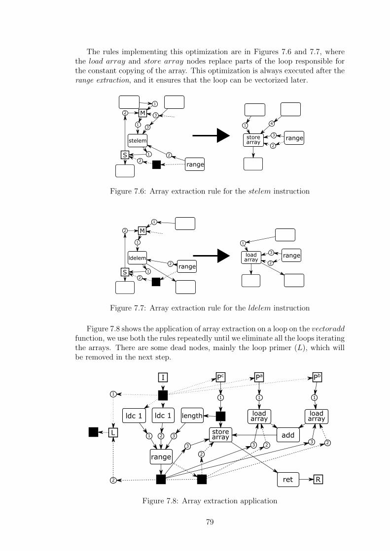
The rules implementing this optimization are in Figures 7.6 and 7.7, wherethe load array and store array nodes replace parts of the loop responsible forthe constant copying of the array. This optimization is always executed after therange extraction, and it ensures that the loop can be vectorized later.

M

S

3

1

2

1

2

stelem

1

range

rangestorearray

2

3 1

2

3

4

Figure 7.6: Array extraction rule for the stelem instruction

M

S

1

2

1

2

ldelem

1

range

rangeloadarray

2

1

2

3

Figure 7.7: Array extraction rule for the ldelem instruction

Figure 7.8 shows the application of array extraction on a loop on the vectoraddfunction, we use both the rules repeatedly until we eliminate all the loops iteratingthe arrays. There are some dead nodes, mainly the loop primer (L), which willbe removed in the next step.

L

1

2

ldc 1

range

1 2

1

2

ret

I

R

ldc 1

Pc

length

1

2

Pa

1

2

Pb

loadarray

loadarray

addstorearray3

333

Figure 7.8: Array extraction application

79

Listing 7.2: Store array node

void s t o r e a r r a y ( stream in1 , stream in2 , stream in3 ,stream in4 , stream out1 )

{while ( ! in1 . e o f ( ) ){

var a r r = in1 . next ( ) ;while ( in2 . next ( ) ){

ar r [ in3 . next ( ) ] = in4 . next ( ) ;}out1 . put ( a r r ) ;

}}

Listing 7.3: Load array node

void l o ad a r ray ( stream in1 , stream in2 , stream in3 ,stream out1 , stream out2 )

{while ( ! in1 . e o f ( ) ){

var a r r = in1 . next ( ) ;while ( in2 . next ( ) ){

out2 . put ( a r r [ in3 . next ( ) ] ) ;}out1 . put ( a r r ) ;

}}

Pseudo-code implementation of the custom operations is in the following list-ings, store array is in Listing 7.2 and the load array is in Listing 7.3.

7.6 Token Extraction

Once all the arrays are extracted, we must make sure that the Tokens are dis-tributed properly even when the loop is later vectorized. This means that wemust replace the loop infrastructure for the Tokens with a vectorizable node thatproperly distributes the tokens according to the range node.

The rule implementing this optimization is in Figure 7.9, we just remove thecast node connected to the loop primer node and add a token cast node connectedto the range node. This way we connect the last of the loops infrastructure tothe range node and the loop primer can be safely removed.

80

L2

1

range L2

1

range

tokencast

Figure 7.9: Token extraction rule for the cast special operation

[add|mul|

sub|div]*storearray

token?cast

load+

array

1

2

1

$11

2

vector1

3

3

range vector1v-storearray

v-tokencast

v-load+

array

1

2

1

3

3

v-range

Figure 7.10: Vectorization rule

7.7 Vectorization

Finally, we introduce the vectorization to further improve the performance of thegraph. Vectorization is almost impossible to use when a graph contains controlflow nodes, because consecutive values may take different paths in the graph,which would break the vectors. However, the custom operations introduced bythe optimizations are fully predictable and if they replace all the control flow ofa loop then we can vectorize that loop.

This optimization takes the body of a loop, which has been completely trans-formed into custom operations, and transforms it into a single vectorized customoperation, unless it contains another nested loop or branch. The rule implement-ing the optimization is in Figure 7.10, where the loop body is replace with a newcustom operation (vector1 in the example), unlike the other optimization, wherewe use a predefined custom operation designed specifically for the situation.

We illustrate the process on the vectoradd function. We take the hybrid flowgraph representing the function and apply all the component extraction-basedoptimizations, the resulting graph is in Figure 7.8. Then we eliminate all thedead nodes and once the loop is completely removed, we can batch the data sothat the range, load array and store array operations can process and producedata in vectors containing parts of the arrays not just single elements. We usethe vectorization optimization to replace the loop with vectorized versions of theoperations, which use vector instructions, like mm add epi32(v1, v2) in SSE. Thecompletely optimized hybrid flow graph is in Figure 7.11.

7.8 Array Extraction and Vectorization Chain-

ing

We can further modify the array extraction and vectorization so they can bechained one after another. First, we introduce the chained vectorization opti-mization, by allowing the output to be a ldelem operation in a proper format.

81

ldc 1

v-range

1 2

1

2

ret

I

R

ldc 1

Pc

length

1

2

Pa

1

2

Pb

v-loadarray

v-loadarray

vectoradd

v-storearray3

333

Figure 7.11: Fully optimized and vectorized vectoradd function

[add|mul|

sub|div]*ldelem+

token?cast

load+

array

1

2

2

$11

2

vector1

3

3

range vector1

v-tokencast

v-load+

array

1

2

2

3

3

v-range

1M

ldelem+

1M

Figure 7.12: Modified vectorization rule

Figure 7.12 shows the modification, where the ldelem operation is required to bedirectly connected to the merge operation to ensure that there is no broadcast.Broadcast would meant that the array is accessed more than once in the loop andcannot be optimized due to potential data dependences.

Next, we introduce the chained array extraction optimization, which supportsother custom operations as a source of the array index, not just the range oper-ation. The rule is in Figure 7.13.

M

S

1

2

1

2

ldelem

1

rangerange

loadarray

2

1

2

3customcustom

Figure 7.13: Array extraction rule for the ldelem instruction

82

8. Compiler Back-end

The compiler back-end transforms the optimized hybrid flow graph to a platformspecific code. It must produce all the components necessary to execute the ap-plication in the environment, which usually means a machine code or byte code,but streaming environments are more complex. They require en execution planand kernel implementations, usually in different language.

We present all the platforms currently supported by our compiler in Sec-tion 8.2. The following sections describe the specific back-end implementationsfor each platform.

8.1 Related Work – Compiler Back-end

The compiler back-end transforms the intermediate code into the code for thetarget platform. The standard practice is to transform the optimized intermedi-ate code into machine or byte code and apply platform-specific optimizations toproduce application best suited for the target environment [57].

The ParallaX compiler back-end transforms an optimized Hybrid Flow Graphinto a Bobox application. We cannot implement the back-end of the compiler inthe standard, straight-forward way, because the applications for Bobox frameworkmust contain both an execution plan and the code of all used kernels (boxes)[2]. The beck-end is divided in two parts: component transformation and planconstruction.

First we transform the subgraph representing the components, created usingthe component extraction, into C++ classes. The native implementation of theBobox system supports kernels implemented as C++ classes [2] and the managedimplementation uses C#. The process is similar to the call graph analysis [85],where the subgraph nodes represent procedures.

The Hybrid Flow Graph structure is very similar to the Bobox execution plan.We transform the top layer of the optimized HFG directly into Bobolang [3]. Theprocess requires only the export of the graph in the correct Bobolang notation.

The produced application must be compiled with the Bobox runtime, whichloads both the kernels and the execution plan and executes the application. TheBobox system creates a memory representation of the execution plan, instantiatesthe used kernels (boxes) and executes the plan. This process is similar to themodern dynamic languages, like C#, where the source code is compiled into anintermediate byte code, which is later executed by a CLR runtime [30].

The back-end traditionally performs platform-specific optimization [57, 36],but we can skip this step, because the optimizations are performed by the C++compiler (for the boxes) and the Bobox environment (for the execution plan) [2].

8.2 Supported Environments

The compiler currently supports four target platforms. Each platform requiresits own back-end implementation that is able to produce all the necessary com-ponents for the final application.

83

The compiler supports the native and managed implementation of the Boboxstreaming system. Both implementations have similar basics and the main differ-ence is supported language for the kernel implementation. The native implemen-tation requires kernels implemented as C++ classes with the basic box (providedby Bobox) as the base class, while the managed implementation uses C#. Bothenvironments require an execution plan implemented in the Bobolang declarativelanguage [3].

The compiler is able to parallelize the C# application directly by embeddingthe managed Bobox directly into the application assembly. The methods aretransformed into plans, executed by the embedded Bobox.

The last currently supported platform are the .NET asynchronous methods.The asynchronous methods internally create a graph of parallel tasks executedby the .NET runtime. The HFG structure is similar to that of an applicationimplemented using asynchronous methods, with the nodes representing separatemethods and edges representing calls and we use this similarity to transform thehybrid flow graph to the asynchronous methods.

8.3 Bobox Transformation

The Bobox system is our main target environment and the back-end for Boboxperforms two main operations. We transform the application HFG directly intoa Bobox plan and then we add custom operations created by the componentextraction. Component extraction groups the bodies of optimized loops into singlevectorized operations.

All the kernels, based on CIL instructions, are already implemented in alibrary attached to Bobox. The custom operations must be handled separately,because we must provide Bobox with their implementation. They are transformedinto a C++ class and attached to the Bobox system, which is then compiled intothe final application. This approach allows us to generate C++ code and theC++ compiler performs all the necessary optimizations.

The transformation is the same for both the native and managed implementa-tion of Bobox, the only difference is the programming language used to implementcustom operations, C++ for native and C# for managed. The native imple-mentation is our main platform, because it is more optimized for data intensiveapplications. The managed implementation is used mainly for testing.

8.4 Transformation Overview

Transforming the HFG into a Bobox plan is a straight-forward process and if thereare no custom operations then the plan is the only thing necessary to completethe application, because the standard operations are already implemented in alibrary attached to Bobox.

The Bobox execution plan must be implemented in the Bobolang declarativelanguage, which is described in detail in Section 2.2. The plan is divided intotwo sections, kernel and stream declaration. Kernels are declared along withtheir type, unique name, parameters, inputs and outputs (including their unique

84

identifiers). Streams connects declared kernels including the identification of aspecific input or output, if the kernels have more than one.

It is important to note that we include in the HFG input nodes, which alwaysrepresent the inputs of other nodes, perform no action and contain only identifierand data type. The inputs are added for all other nodes and every edges has eitherinput as a source or a sink. The input nodes are used in the transformation foBobolang to match the stream inputs and outputs and they are removed in theprocess.

8.5 Execution Plan Construction

Algorithm 15 Hybrid flow graph transformation to Bobolang plan

Require: G – source HFGEnsure: B – Bobolang plan1: B := ”operatormain()− > (){”2: for all n ∈ N(G) do3: IN := {i ∈ N(G) : (i, n) ∈ E(G)}4: INPUTS := ””5: for all i ∈ IN do6: INPUTS := INPUTS + ”({i.TY PE})[i {i.ID}]”7: end for8: OUT := {o ∈ N(G) : (n, o) ∈ E(G)}9: OUTPUTS := ””10: for all o ∈ OUT do11: OUTPUTS := OUTPUTS + ”({o.TY PE})[o {o.ID}]”12: end for13: B := B + ”{n.ANNOTATION}{INPUTS} → {OUTPUTS} {n.ID}; ”14: end for15: for all e ∈ {ed ∈ E(G) : e.SINK.ANNOTATION = Input} do16: ID := e.SINK.ID17: B := B + ”{e.SOURCE}[o {ID}]→ {e.SINK}[i {ID}]”18: end for19: B := B + ”}”

Algorithm 15 shows the entire transformation process using the C# stringnotation, where the {X} part is replaced in the final string by the value of X.The algorithm first transforms nodes to Bobolang kernels, where we omitted thekernel parameters, since they are used only for the constants to indicate theirvalues. Next, we transform the edges that connect a node through an input toanother node, we use the input to match the stream ends.

The transformation is best demonstrated on an example, we take a small HFGand transform it to Bobolang plan. We transform the right graph in Figure 8.1and the produced Bobolang plan is in Listing 8.1. In the graph, we omit inputnodes for nodes with only one input and we perform the component extractionoptimization described in Section 7.2, which replaces the arithmetical nodes witha custom operation.

85

sub

mul

addldc 1

ret

I Pa

ldc 1

ret

I Pa

custom

1

2

Figure 8.1: Optimized vector addition HFG

operator main()−>() {Star t ()−>( token ) [ o 6 ] s t a r t 0 ;Ldc ( token ) [ i 7 ]−>( i n t ) [ o 9 ] l d c 1 ( 1 ) ;Ldarg ( token ) [ i 8 ]−>( i n t ) [ o 10 ] l d a rg 2 (” a ” ) ;Ret ( i n t ) [ i 1 1 ]−>() r e t 3 ;broadcast ( token ) [ i 6 ]−>( token ) [ o 7 ] , ( token ) [ o 8 ] broad 4 ;CustomBody( i n t ) [ i 9 ] ( i n t ) [ i 1 0 ]−>( i n t ) [ o 11 ] custom 5 ;

s t a r t 0 [ o 6 ] −> [ i 6 ] broad 4 ;broad 4 [ o 7 ] −> [ i 7 ] l d c 1 ;broad 4 [ o 8 ] −> [ i 8 ] l d a r g 2 ;l d c 1 [ o 9 ] −> [ i 9 ] custom 5 ;l d a r g 2 [ o 10 ] −> [ i 1 0 ] custom 5 ;custom 5 [ o 11 ] −> [ i 1 1 ] r e t 3 ;}

Listing 8.1: Bobolang plan produced from the HFG in Figure 8.1

All the nodes in the Bobox plan are standard instruction kernels provided byour library or broadcasts built in Bobox, the only exception is the CustomBodynode produced by the component extraction. This kernel has to be crated by thecompiler back-end and provided along with the plan, which is explained in thenext section.

8.6 Component Extraction

Component extraction is an optimization defined in Section 7.2, which reducescommunication overhead of the final application by grouping multiple HFG nodesinto a single custom node.

A graph without control flow can be directly transformed into a single customoperation with semantics defined by a C++ function. The transformation isperformed in two steps. First, we sort the HFG nodes topologically and thenwe transform each node into a method call, one after another. The topologicalordering makes sure that all the methods are called in correct order.

Figure 8.2 shows an example of the transformation, where the graph is topo-logically ordered top-to-bottom and left-to-right. The produced code calls onlytiny methods representing CIL instructions, which are attached as a library andinlined by the C++ compiler.

Algorithm 16 transforms a HFG without control flow nodes to a C++ func-tion. The algorithm constructs the code directly from nodes, where each node isrepresented by a call to a tiny function. We use C# string notation to build the

86

ldc 3

mul

add

ret

ldc 5 ldloc aauto in1 = ldc(5);

auto in2 = ldloc(a);

auto in3 = add(in1, in2);

auto in4 = ldc(3);

auto in5 = mul(in3, in4);

return in5;

Figure 8.2: Transformation of a graph without control flow

Algorithm 16 Component transformation algorithm

Require: G – source HFGEnsure: C – C++ code (sequence of statements)1: C := ””2: NODES := topology sort(G)3: REG := ∅4: X := 05: for all node ∈ NODES do6: REG[X] := node7: IN := {”in” +REG[n] : n ∈ NODES ∧ (n, node) ∈ E(G)}8: S := ”auto in{X} = {annotation(node)}({join(′,′ , IN)})”9: C := C + S10: X := X + 111: end for

statements, where the {X} is replaced by the value of X.In the Bobox environment, this requires that we create a new kernel class and

compile it into the final application. We use Algorithm 16 to produce the codefor the custom box. We can do this, because we perform the optimization onlyon the bodies of optimized loops that do not contain any control flow nodes. Weproduce code that uses only the basic instructions implemented as tiny functionsimmediately inlined by the compiler, which does not limit performance.

Once we have the source code for the kernel body, we create the class rep-resenting the kernel. This class is always very similar, the only difference is theBody method and the input / output streams. We transform the HFG to thesource code of the Body method and add the rest of the class implementation.We omit the actual algorithm as its only job is to generate the input and outputstream names and copy the body code.

Listing 8.2 shows the implementation of the custom kernel used in Figure 8.1.The Body method implements the component showed in the left graph in Fig-ure 8.1, which is then extracted and replaced by the custom node, shown in theright graph.

87

class merge box : public bas i c box {public :

typedef gener ic mode l<merge box> model ;

BOBOX BOX INPUTS LIST( in1 , 0 , in2 , 1 ) ;BOBOX BOX OUTPUTS LIST( out , 0 ) ;

merge box ( const box parameters pack &box params ): bas i c box ( box params )

{}

virtual void sync body ( ) o v e r r i d e{

input stream<int> in1 ( this , inputs : : in1 ( ) ) ;input stream<int> in2 ( this , inputs : : in2 ( ) ) ;output stream<int> out ( this , outputs : : out ( ) ) ;

while ( ! in1 . e o f ( ) && ! in2 . eo f ( ) ) {int l = in1 . cur r ent ()−>get <0>();int r = in2 . cur r ent ()−>get <0>();out . next()−>get<0>() = Body( in1 , in2 ) ;

}}

int Body( int in1 , int in2 ){

auto i 1 = add ( in1 , in2 ) ;auto i 2 = sub ( in1 , in2 ) ;auto i 3 = mul ( i1 , i 2 ) ;return i 3 ;

}} ;

Listing 8.2: Implementeation of the custom kernel in Figure 8.1

88

9. Additional Environments

The ParallaX compiler contains multiple back-end implementations that providethe support for other platforms, besides the managed and native implementationof the Bobox streaming environment. The compiler also supports the .NET asyn-chronous methods and a direct integration of the managed Bobox system. In thischapter, we will explain the basics of the other platforms and we will describethe implementation of the respective back-ends.

9.1 .NET Asynchronous Method

The asynchronous methods are parallel methods managed by the .NET frame-work. The methods are implemented and called as synchronous methods, butinstead of immediately calculating their result, they return a task object thatcontains the information about the ongoing calculation. The framework intro-duces the await operator that pauses the caller, until the given task is completedand then it returns the result.

The asynchronous methods are designed to mainly improve responsiveness andthroughput of applications that require time consuming operations, like networkcommunication. They are not well suited to parallelization of calculation heavyor data intensive applications. As such, we use this platform mainly for testingand evaluation.

9.1.1 Transformation Overview

The back-end for this platform transforms a HFG into a C# code composed ofasynchronous methods. The transformation process must handle three cases – asubgraph without control flow, a branch (split-merge) infrastructure and a loop(merge-split-primer) infrastructure. First, we explain the entire algorithm andthen we introduce the three separate steps.

All the CIL instructions are implemented as asynchronous methods in a libraryattached to the produced code, so they can be used directly.

Algorithm 17 transforms an input HFG info a C# code containing a listof methods representing the control-flow constructs and a single main method,which is an entry point to the produced code. The algorithm uses procedures thattransform loops, branches and graphs without control-flow, which are defined inthe following sections along with the pattern graphs LOOP and BRANCH. Be-sides the transformation procedures, we us additional helper procedures describedin the following list:

• copy – creates a deep copy of a graph

• match – matches an associative graph rewriting rule (see Section 3.1.1)

• replace – replaces a subgraph by a single node with the given annotation

89

Algorithm 17 HFG transformation to asynchronous methods

Require: G – source HFGLOOP – loop pattern graphBRANCH – branch pattern graph

Ensure: C – C# code (set of methods)1: C := ∅2: H := copy(G)3: X := 04: M := ∅5: while Split ∈ N(H) do6: if match(LOOP,H,M) then7: C := C ∪ {LoopToMethod(G,M, ”loop” +X)}8: H := replace(M, ”loop” +X)9: else if match(BRANCH,H,M) then10: C := C ∪ {BranchToMethod(G,M, ”branch” +X)}11: H := replace(M, ”branch” +X)12: end if13: X := X + 114: end while15: C := C ∪ {ToMethod(H, ”main”)}

9.1.2 Graph Without Control-Flow

A hybrid flow graph does not contain any control-flow constructs, when it containsno split or merge nodes. Without control-flow a HFG can be directly transformedinto a C# method the same way we transform the subgraphs after the componentextraction in the Bobox back-end.

We use the procedure ToMethod to transform a HFG without control-flow toa single C# asynchronous method. The method is implemented using a modifiedversion of Algorithm 16 defined in the previous chapter (Section 8.6). A slightmodification is necessary for the algorithm to produce C# code instead of C++,we replace the variables automatic type auto by the C# equivalent var.

9.1.3 Branch Transformation

The branch pattern graph shown in Figure 9.1 matches the infrastructure in-cluding the conditional jump and the bodies of both branches, where we do notuse the traditional notation for split and merge so we can add the plus signmeaning repetition in the associative graph rewriting systems. The bodies areHFG subgraphs, without any control flow nodes that can be transformed by theToMethod procedure. Iterative application of the algorithm ensures, that nestedbranches and loops are replaced from the inside of the nest out, starting withconstructs containing no embedded control flow.

Algorithm 18 transforms the subgraph matched by the pattern graph in Fig-ure 9.1 to a single asynchronous method, which is then added to the final code.The subgraph is then replaced by the method name.

Figure 9.2 shows the transformation of a simple branch subgraph matched bythe patter graph. The transformation produces a single asynchronous method

90

[^split|

merge]* merge+split+

[blt|bgt|...]

[^split|

merge]*

Figure 9.1: Branch pattern graph

Algorithm 18 BranchToMethod algorithm

Require: G – original HFGM – matched HFG subgraphN – method name

Ensure: C – C# code (method)1: IN := {”p{i.ID}” : i ∈ N(M) ∧ ∃(n, i) ∈ E(G)→ n /∈ N(M)}2: OUT := {”p{o.ID}” : o ∈ N(M) ∧ ∃(o, n) ∈ E(G)→ n /∈ N(M)}3: C := ”async void {N}({join(′,′ , IN)}, out {join(′, out′, OUT )}){”4: C := C + ”if({ToMethod(M.JUMP )}){”5: C := C + ToMethod(M.BODY TRUE)6: C := C + ”}else{”7: C := C + ToMethod(M.BODY FALSE)8: C := C + ”}}”

that is called by the other methods produced from the HFG.

9.1.4 Loop Transformation

The loop transformation is similar to the branch, but the final method is recur-sive to accommodate the loop behavior. A loop can be transformed to either aC# loop or recursion, where the recursion allows the separate iterations to runin parallel, if they are independent, taking an advantage of the asynchronousbehavior.

Pattern graph in Figure 9.3 matches an array infrastructure including itsconditional jump and body. The loop body does not contain any other controlflow constructs.

Algorithm 19 transform the matched loop subgraph to a recursive asyn-

S

1

2

blt

M

1 2

inc

3

dec

async void branch1(int p1, out int p2)

{

if(blt()) {

p2 = inc(p1);

} else {

p2 = dec(p1);

}

}

Figure 9.2: Branch transformation

91

[^split|

merge]*split+merge+

[blt|bgt|...]L

Figure 9.3:

Algorithm 19 LoopToMethod algorithm

Require: G – original HFGM – matched HFG subgraphN – method name

Ensure: C – C# code (method)1: IN := {”p{i.ID}” : i ∈ N(M) ∧ ∃(n, i) ∈ E(G)→ n /∈ N(M)}2: OUT := {”p{o.ID}” : o ∈ N(M) ∧ ∃(o, n) ∈ E(G)→ n /∈ N(M)}3: C := ”async void {N}({join(′,′ , IN)}, out {join(′, out′, OUT )}){”4: C := C + ToMethod(M.BODY )5: C := C + ”if({ToMethod(M.JUMP )}){”6: C := C + ”{N}({join(′,′ , IN)}, out {join(′, out′, OUT )}); ”7: C := C + ”}else{”8: for all I ∈ IN ∧O ∈ OUT do9: C := C + ”{I} = {O}; ”10: end for11: C := C + ”}}”

chronous method. The algorithm is a bit simplified in regarding the parameterspassing, where the inputs and outputs are matched, because every merge-splitpair represents a single variable. The process is illustrated in Figure 9.4, where asimple loop is transformed according to the algorithm.

M

1 3

bgt 0

S1

dec

2

2

L

async void loop1(int p1, out int p2)

{

p1 = dec(p1);

if(bgt0(p1))

{

loop1(p1, out p2);

} else {

p2 = p1;

}

}

Figure 9.4: Loop transformation

9.2 Managed Bobox Integration

The last currently supported target platform is an integrated managed Bobox. Inthis setup, the compiler integrates the managed Bobox directly into the optimized

92

application, which is transformed into HFG and then to Bobox plan for the Boboxto execute. The process overview is in Figure 9.5. This platform was implementedas the original proof of concept and it is not optimized for efficiency.

application

compiler HFG

optimized

application

graph

register

Bobox

Figure 9.5: Application parallelization overview

The compiler transforms the application methods to HFGs and replaces theiroriginal code with a simple command that executes the produced plan by Bobox.The compiler also adds a graph register, which efficiently stores all the HFGstransformed to Bobox plans. Bobox is attached as a dynamic library to theapplication so it can be used to execute the plans.

The compiler creates an application that produces the same outputs as theoriginal, but its methods are implemented in HFGs transformed in Bobox plans.

9.2.1 Graph Execution

Bobox computation is defined by an execution plan that is very similar to a hybridflow graph, it is also an annotated directed graph. We have designed an adapterthat transforms a HFG to a Bobox plan which is then executed by Bobox. Theadapter is part of the graph register that stores all the HFGs and executes themin Bobox.

A HFG is basically identical to a Bobox execution plan, but it requires specifickernels to be executed, because Bobox must have access to the operations assignedto each node. We must provide a set of kernels for all CIL instructions and allcontrol flow nodes. The kernels are already part of the Bobox library attachedto the optimized application.

Once all the kernels are available, we simply convert each HFG to a planby transforming each node to an appropriate kernel and connecting the kernelsaccording to the edges.

The source HFG is transformed to a Bobox plan and stored in a graph register(see Section 9.2.2). This way we are able to execute the HFG efficiently andrepeatedly, which is necessary for methods called in a loop or similar.

9.2.2 Graph Integration

We use the compiler front-end presented in Section 6 to transform the methodsto HFGs. The Produced graphs are stored in the graph register, which is used bythe rest of the application to execute them via Bobox. The resulting structure ofthe application is in Figure 9.6, in an UML-like notation.

The resulting parallel application contains some of its original code, paral-lelized methods, a graph register and a Bobox library. Which methods are par-allelized is driven by the configuration described in Section 12.1. The register

93

Figure 9.6: Structure of the parallelized application

contains a list of graphs, one for each parallelized method, and an instance ofthe Bobox environment. The compiler provides configuration tools that allowusers to specify which methods are parallelized and it automatically integratesmethods before parallelization.

The register is a singleton injected into the application by the compiler. Itscode is in Listing 9.1. The graphs are stored in the register in the variablegraphRegister, where they are inserted in the Initialize method. The graphsare initially stored as strings and in the Initialize method, they are transformedinto a binary representation, optimized for efficient execution. The register ini-tialization is performed only once when the application starts.

Listing 9.1: Graph register

public stat ic class GraphRegister{

stat ic Bobox . Scheduler s chedu l e r ;stat ic List<Tuple<Box [ ] , ModelInstance>> graphReg i s te r ;stat ic bool i n i t i a l i z e d = fa l se ;stat ic sbyte methodCounter ;

private stat ic Scheduler Scheduler{

get{i f ( s chedu l e r == n u l l )s chedu l e r = new Bobox . S e r i a l S c h e d u l e r ( 1 ) ;return s chedu l e r ;}

}

private stat ic void I n i t i a l i z e ( ){i n i t i a l i z e d = true ;Logger . debug out = fa l se ;g raphReg i s te r = new List<Tuple<Box [ ] , ModelInstance >>();

FlowGraph graph = FlowGraph . Dese r i a l i z eFromStr ing ( ”” ) ;ModelInstance in s t ance = new ModelInstance ( ) ;Box [ ] i n t e r f a c e = f low graph . BuildPlan ( graph , i n s t anc e ) ;g raphReg i s te r . Add( i n t e r f a c e , i n s t anc e ) ;

94

}

public stat ic void ExecuteGraph ( int id ){i f ( ! i n i t i a l i z e d )

I n i t i a l i z e ( ) ;Scheduler .Go( graphReg i s te r [ id ] . Item2 ) ;}

public stat ic Bobox . Box [ ] GetInputOutput ( int id ){i f ( ! i n i t i a l i z e d )

I n i t i a l i z e ( ) ;return graphReg i s te r [ id ] . Item1 ;}

}

The Bobox environment is also managed by the graph register. The registeruses the C# implementation of Bobox. The environment is represented by thevariable scheduler that contains the scheduler that manages the Bobox executionplans. The graph register provides the ExecuteGraph method which submitsselected graph to the scheduler that executes it.

The parallelized methods are replaced by a short code that uses the registerto execute the HFG constructed from their original code. The replacement codeof the method is in Listing 9.2.

Listing 9.2: Method replacement

{int id = 0 ;Box [ ] param = register . GraphRegister . GetInputOutput ( id ) ;( param [ 2 ] as param<Int32 >). Value = P;( param [ 1 ] as l d c i 4 r e p e a t ) . Repeat = 1 ;register . GraphRegister . ExecuteGraph ( id ) ;return ( param [ 0 ] as ret<Int32 >). AcceptedValues . F i r s t ( ) ;

}

The replaced method must do only three things - provide parameters for thegraph (based on its actual parameters), execute the graph and obtain the returnedvalue. In the code in Listing 9.2, the first four lines prepare parameters, callingthe ExecuteGraph executes the graph using the parallel environment and thelast line returns the value produced by the graph.

95

96

10. Case Study: Matrix-basedDynamic Programming

In the previous chapters, we presented the ParallaX compiler for streaming en-vironments that transforms a C# application to an application for the Boboxstreaming system. In this chapter, we will focus on the basic problem of edit dis-tance, the Levenshtein distance, that will serve as a case study for the compiler.The Levenshtein distance calculates the number of changes necessary to maketwo strings equal, thus calculating their relative similarity.

The structure of the algorithm calculation, shown in Figure 10.1, severelylimits any available parallelism. To improve this situation, the author of this work,as a member of a wider research team, has developed a special optimization thatrestructures the calculation to blocks that offer parallelism, suitable for vectorinstructions.

The author of this work designed the blocked Levenshtein distance algorithmalong with two colleagues and the algorithm was initially published with GPU-specific optimizations [8] and then in a wider study that added Intel Xeon Phi andCPU optimization [2]. In the team, the author was responsible for the algorithmoptimization for the GPUs. In the collaborative work, we described optimizationsgreatly improving the application of SIMD instructions and the main principlesare described in the following sections.

The Levenshtein distance is just one problem of the matrix-based dynamicprogramming class. A similar problem that uses dynamic programming is dy-namic time warping (DTW) defined by Muller [87]. Since the performance issueis also quite important for DTW applications, Sart et al. discussed parallelizationtechniques for GPUs and FPGAs [88]. They focused mainly on a specific versionof DTW algorithm, which reduces the dependencies of the dynamic programmingmatrix, thus allows more efficient parallelization. Another example of a problemsuitable for dynamic programming is the Smith-Waterman algorithm [89], whichis used for protein sequences alignment. One of the first attempts to parallelizethis algorithm on GPUs was made by Liu et al. [90].

We evaluate the ParallaX compiler correctness and efficiency on the blockedversion of Levenshtein distance and compare the results to its serial C# imple-mentation. The compiler must correctly transform the application to a streamingprocessing application and then add the necessary kernel and vector parallelismto improve its performance.

The rest of this chapter describes the blocked algorithm and its parallelizationby our compiler. In Section 10.2 we explored other approaches to optimize theLevenshtein distance. Section 10.1 explains the distance algorithm and its prop-erties. In Section 10.3 we present the details of the blocked version of Levenshteindistance. In Section 10.4 we adapt the blocked algorithm for streaming environ-ments and in the next chapter, we present thw experiments with the applicationsproduced by our compiler.

97

10.1 Problem Details

In the original research, we have selected the Wagner–Fischer dynamic program-ming algorithm [91] for the Levenshtein distance problem as a representative forour implementation since its computational simplicity emphasizes the communi-cation and synchronization overhead associated with parallel computations. Inthis work, we use the blocked Levenshtein distance to evaluate the ability of theParallaX compiler to exploit parallelism in a complex algorithm that providesopportunities for vectorization.

In the matrix-based dynamic programming algorithms, the values vi,j of thematrix are calculated recursively based on algorithm-specific function f(i, j). TheFunctions f(i, j) employed in these calculations are often very simple. In thecase of the Wagner-A–Fischer dynamic programming algorithm [91] for the Lev-enshtein distance, the function involves only comparison, incrementation, andminimum:

f(i, j) = min(vi−1,j + 1, vi−1,j−1 + 1− δv[j]u[i] , vi,j−1 + 1),

where the Kronecker δ compares the i-th and j-th positions in the input stringsu and v respectively.

The dependencies between individual invocations of the formula f significantlylimit the parallelism available in the problem. For a M ×N matrix (i.e., inputsof size M and N respectively), at most min(M,N) elements may be computed inparallel using the diagonal approach illustrated in Figure 10.1. Therefore, whenthe computation of f does not take orders of magnitude more time than the dataexchange, a pure diagonal approach cannot be effectively employed on currentCPU and GPU architectures, because it would require global synchronizationafter every diagonal is processed.

current iteration

previous iteration

the iteration before last

Figure 10.1: Dependencies in the matrix and the diagonals

On the other hand, the diagonal approach gives us basis for processing sub-sections of the distance matrix using SIMD instructions (in case of CPU and IntelXeon Phi) or threads running in lockstep (in case of GPU). Although possible, thediagonal approach still produces insufficient parallelism and unnecessary memorytransfers, because the diagonals must be constantly rotated through the SIMDregisters. In Section 10.3 we present a special transformation that divides the al-gorithms matrix into block, which can be processed directly by SMID instructionswithout unnecessary memory operations.

98

10.2 Related Work – Matrix-based Dynamic

Programming Parallelization

The algorithm and optimizations presented in this chapter are based on our previ-ous work focusing on the parallelization of the matrix-based dynamic algorithmson GPUs [8] and out next research that further extended the optimizations toencompass Intel Xeon Phi [2]. Both our previous works focused on the vector-ization capabilities of the respective accelerators. In this work, we transfer theoptimizations to the environment of streaming systems using the ParallaX com-piler described in the previous chapters.

Most parallel algorithms are based on an observation of Delgado et al. [92],who studied the data dependencies in the dynamic programming matrix. Twopossible ways of processing the matrix were defined in their work – uni-directionaland bi-directional filling. The original idea allows limited concurrent processing,but it needs to be modified for massively parallel environment.

One of the first papers that covers the whole issue of the parallelization ofLevenshtein distance on GPUs was presented by Tomiyama et al. [93]. Theirapproach divides the dynamic programming matrix into parallelogram blocks.Independent parallelograms are computed by separate CUDA thread blocks whileeach block is computed in a highly cooperative manner. The main focus ofthe work addressed the problem of appropriate block size and its automaticalselection. On the other hand, their experiments are currently out of date, sincethey were performed on a GPU with compute capability 1.3 only.

Manavski et al. [94] reimplemented the Smith-Waterman algorithm using CU-DA technology. Slightly different solution was presented by Ligowski et al. [95].Their work focused on searching in the entire database of proteins. Khajeh-Saeedet al. [96] utilized the computational power of multiple GPUs to solve this prob-lem. Perhaps the most recent version was presented again by Liu et al. [97] andit combines observations from the previous work.

10.3 Levenshtein Distance Blocked Algorithm

As illustrated by Figure 10.2, the dependencies between elementary calculationsin the two-dimensional matrix allow parallel computation for all elementary taskson any diagonal line. An elementary task is consists of evaluation of the functionf(i, j) producing the value for a single element of the algorithm matrix. Thus, thecomputation may be done by a single sequential sweep through all the diagonalsin the matrix whilst each diagonal is computed in parallel. Unfortunately, suchsimple approach to parallelization suffers from two deficiencies: First, the size ofthe diagonal (n) varies throughout the matrix which requires frequent additionand removal of computing units (threads) during the sweep. Second, regardlessof the exact assignment of the physical threads to the elementary tasks, eachthread processing a task must interchange information with at least one otherthread when the computation advances to a subsequent diagonal. The compu-tational cost of the elementary tasks is assumed to be small, thus the threadcommunication cost plays an important role as well.

When more than one instance of the problem is computed simultaneously, it is

99

Figure 10.2: A single block with emphasized input, output, and data dependencies

also possible to compute the instances in parallel while each instance is evaluatedsequentially (e.g., row-wise). However, this approach suffers from the inability toutilize the SIMD while efficiently using the caches.

Thus, although the multi-instance problem seems to be embarrassingly par-allel, non-trivial algorithms must be investigated to overcome the memory andSIMD instruction constraints.

10.3.1 Parallelogram Blocks

Due to the nature of data-dependencies in the computation matrix, SIMD in-structions work best when assigned to parallelogram-like portions of the matrix,as depicted in Figure 10.2. The picture also shows the input values for such ablock, divided into left buffer (red), upper-left buffer (blue), and upper buffer(green). The arrows show the dependencies for the first diagonal in the blockwhich will be computed in parallel. The output of the parallelogram block isshown in light gray, the white fields inside the parallelogram correspond to tem-porary values computed and later discarded during the block evaluation.

Each block is processed in three steps: load input data from the memory toSIMD registers, compute the values, and write the results back to the memory forthe subsequent blocks. A block of height H and width W , with H equal to theSIMD register size (4 for SSE and 8 for AVX), is processed by SIMD instructionsin W iterations. Between subsequent iterations, data is shuffled in the registers.

If H is bigger than the SIMD register size then the data must be processedin multiple SIMD streams, which must exchange data between registers.

Figure 10.3: Distance matrix divided into parallelogram blocks

100

10.3.2 Blocked Algorithm

The elements of the distance matrix are grouped into parallelogram blocks asshown in Figure 10.3, where the numbers denote coarse diagonals. Blocks thatare not completely contained in the distance matrix can be processed the sameway as the others, which allows us to avoid checking any conditions during theblock calculation, which comes at the cost of calculating some values that arenot used. Gray area represents the input values for the left and upper blocksand the black square is the final result (computed edit distance). The blockscommunicate through memory buffers, allocated in advance and aligned to 16bits. The division of the matrix into the blocks follows a similar pattern as in thework of Tomiyama [93].

Similarly to the fine diagonals in Figure 10.2, the coarse diagonals allow paral-lel processing of blocks. Blocks retain the same scheme of dependencies as singleelements, thus the blocks in a coarse diagonal can be processed in parallel, be-cause they depend only on blocks from two previous coarse diagonals. The blocknumbers depicted in Figure 10.3 indicate the order in which they are computed.

Each coarse diagonal of blocks is computed by a group of identical kernels,where each corresponds to a single parallelogram block. Selecting appropriateblock size (i.e., its width and height) is an important factor that affects theefficiency of the algorithm.

10.4 Matrix-based Dynamic Programming in

Streaming Environments

In the previous section, we presented the blocked implementation of the Leven-shtein distance algorithm originally designed for CPUs. In this section, we ex-amine the way the ParallaX compiler transforms the C# implementation of thealgorithm into a streaming application. The blocked algorithm can be adaptedfor other problems that share similar dependences and data structure.

However; we can adapt the optimizations, presented in Chapter 7, to vec-torize the blocked implementation. This allows programmers to optimize theiralgorithm once it has been adapted to the blocked design.

The compiler is able to vectorize the code using the Intel CPU streamingextensions, SSE and AVX, but it can be later extended to other hardware, likeGPUs, once the Bobox system supports it.

10.4.1 Blocked Algorithm Implementation in C#

We start with the blocked version of the Levenshtein distance algorithm imple-mented in C# and we will deconstruct it to explain the necessary optimizations.This is necessary, because the blocked implementation is complex and optimizeis all at once not be practical.

Listing 10.1: Blocked Levenshtein edit distance algorithm

int BlockedLevenshte inDistance ( int [ ] s t r1 , int [ ] s t r2 ,int width , int he ight )

101

{#reg ion I n i t i a l i z a t i o n

var strWidth = s t r 1 . Length ;var s t rHe ight = s t r 2 . Length ;var blockHeight = st rHe ight / he ight ;var o f f se tWidth = blockHeight ∗ ( he ight − 1 ) ;var blockWidth = ( strWidth + of f se tWidth ) / width + 1 ;var maxWidth = width ∗ blockWidth ;var appendixWidth = maxWidth − strWidth ;

int [ ] [ ] p r e l a s t = new int [ b lockHeight ] [ he ight + 1 ] ;int [ ] [ ] l a s t = new int [ b lockHeight ] [ he ight + 1 ] ;int [ ] [ ] cu r r ent = new int [ b lockHeight ] [ he ight + 1 ] ;int [ ] [ ] h o r i z o n t a l = new int [ blockWidth ] [ width + 1 ] ;int [ ] [ ] newhor izonta l = new int [ blockWidth ] [ width + 1 ] ;

Set ( p r e l a s t , MaxValue ) ;Set ( l a s t , MaxValue ) ;l a s t [ 0 ] [ 1 ] = 1 ;Set ( newhor izonta l , MaxValue ) ;

for ( int i = 0 ; i < blockWidth ; i++){

for ( int j = 0 ; j <= width ; j++){

h o r i z o n t a l [ i ] [ j ] = i ∗ width + j ;}

}

#endreg ion // I n i t i a l i z a t i o n

for ( int j = 0 ; j < blockHeight ; j++){

for ( int i = 0 ; i < blockWidth ; i++){

var o f f s e t 1 = of f se tWidth + i ∗width − j ∗( height −1);var o f f s e t 2 = j ∗ he ight ;var newHor = SolveBlock ( width , height ,

r e f p r e l a s t [ j ] , r e f l a s t [ j ] , r e f cur r ent [ j ] ,h o r i z o n t a l [ i ] , newhor izonta l [ i ] ,s t r1 , s t r2 , o f f s e t 1 , o f f s e t 2 ) ;

r e s [ 0 ] = ( i >0)? h o r i z o n t a l [ i − 1 ] [ width ] : MaxValue ;var t = h o r i z o n t a l [ i ] ;h o r i z o n t a l [ i ] = r e s ;newhor izonta l [ i ] = t ;

}

102

}

var pos = of f se tWidth + strWidth ;return h o r i z o n t a l [ pos / width ] [ pos % width ] ;

}

The blocked version of the Levenshtein distance algorithm is implemented inListing 10.1. The implementation uses two additional functions, the function Setinitializes all elements of an array to a specified value and the function SolveBlockcalculates the results for a single parallelogram block. The SolveBlock functionis implemented in Listing 10.2

Listing 10.2: Solve single parallelogram block

int [ ] So lveBlock ( int width , int height ,r e f int [ ] p r e l a s t , r e f int [ ] l a s t , r e f int [ ] current ,int [ ] ho r i z on ta l , int [ ] newHorizontal , int [ ] s t r1 ,int [ ] s t r2 , int o f f s e t 1 , int o f f s e t 2 )

{p r e l a s t [ 0 ] = h o r i z o n t a l [ 0 ] ;int x = 1 ;do{

int nX = x − 1 ;l a s t [ 0 ] = h o r i z o n t a l [ x ] ;int y = 1 ;do{

int nY = y − 1 ;int s1 = o f f s e t 1 + nX − nY;int s2 = o f f s e t 2 + nY;

int char1 = s t r 1 [ s1 ] ;int char2 = s t r 2 [ s2 ] ;int l e f t = l a s t [nY ] ;int upper = l a s t [ y ] ;int u p p e r l e f t = p r e l a s t [nY ] ;

// ParallaXMath p r o v i d e s f u n c t i o n s s i m i l a r to// C# Math , des i gned f o r the Paral laX compi lerint d i s t 1 = ParallaXMath . Min( l e f t , upper ) + 1 ;int d i s t 2 = u p p e r l e f t +

ParallaXMath . NotEquals ( char1 , char2 ) ;cur r ent [ y ] = ParallaXMath . Min( d i s t1 , d i s t 2 ) ;y++;

}while ( y <= he ight ) ;

newHorizontal [ x ] = cur rent [ he ight ] ;

103

var temp = p r e l a s t ;p r e l a s t = l a s t ;l a s t = cur rent ;cur r ent = temp ;x++;

}while ( x <= width ) ;return newHorizontal ;

}

10.4.2 Blocked Algorithm in ParallaX Compiler

The Levenshtein distance calculates the edit distance of two strings, by comparingevery combination of characters in both. In this section, we call strWidth thelength of the first string and strHeight the length of the second one. Thisbasically means that the algorithm fills a matrix with strWidth ∗ strHeightelements and returns the one in the lower right corner.

The blocked algorithm is a nest of four loops, where the outer two loopsiterate over bocks and the inner two loops solve a single block. The vectorizationis centered in the innermost loop, which does most of the actual computationsand is executed the most times. The body of the innermost loop is executed forevery element of the virtual matrix, which means that it is executed strWidth ∗strHeight times.

The outer loops offer no significant opportunity for vectorization (they justswap arrays) and they are executed significantly less times. The SolveBlockfunction is called approximately (strHeight/height) ∗ (strWidth/width), whichis far less that the inner loop body, for reasonably big blocks.

Inner Loop Vectorization

Listing 10.3: Inner loop code

do{

// index computationint nY = y − 1 ;int s1 = o f f s e t 1 + nX − nY;int s2 = o f f s e t 2 + nY;// array l o a d sint char1 = s t r 1 [ s1 ] ;int char2 = s t r 2 [ s2 ] ;int l e f t = l a s t [nY ] ;int upper = l a s t [ y ] ;int u p p e r l e f t = p r e l a s t [nY ] ;// d i s t a n c e computationint d i s t 1 = ParallaXMath . Min( l e f t , upper ) + 1 ;int d i s t 2 = u p p e r l e f t +

104

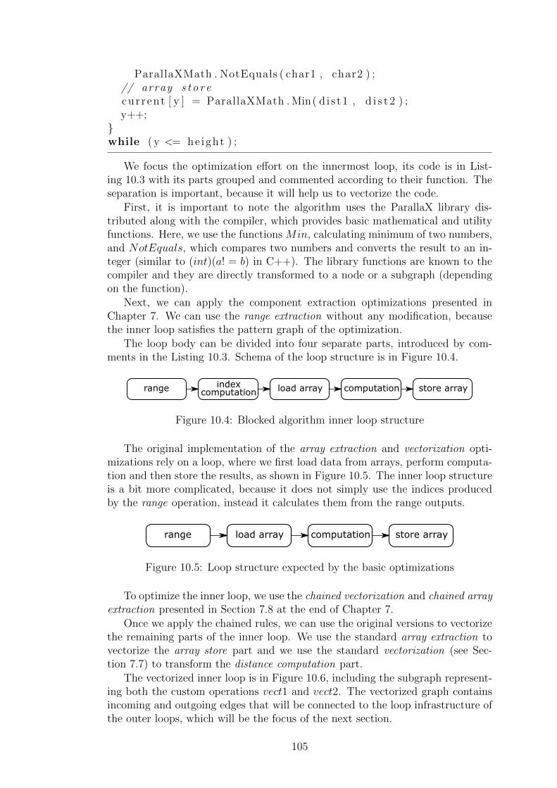
ParallaXMath . NotEquals ( char1 , char2 ) ;// array s t o r ecur r ent [ y ] = ParallaXMath . Min( d i s t1 , d i s t 2 ) ;y++;

}while ( y <= he ight ) ;

We focus the optimization effort on the innermost loop, its code is in List-ing 10.3 with its parts grouped and commented according to their function. Theseparation is important, because it will help us to vectorize the code.

First, it is important to note the algorithm uses the ParallaX library dis-tributed along with the compiler, which provides basic mathematical and utilityfunctions. Here, we use the functions Min, calculating minimum of two numbers,and NotEquals, which compares two numbers and converts the result to an in-teger (similar to (int)(a! = b) in C++). The library functions are known to thecompiler and they are directly transformed to a node or a subgraph (dependingon the function).

Next, we can apply the component extraction optimizations presented inChapter 7. We can use the range extraction without any modification, becausethe inner loop satisfies the pattern graph of the optimization.

The loop body can be divided into four separate parts, introduced by com-ments in the Listing 10.3. Schema of the loop structure is in Figure 10.4.

computationload array store arrayindexcomputationrange

Figure 10.4: Blocked algorithm inner loop structure

The original implementation of the array extraction and vectorization opti-mizations rely on a loop, where we first load data from arrays, perform computa-tion and then store the results, as shown in Figure 10.5. The inner loop structureis a bit more complicated, because it does not simply use the indices producedby the range operation, instead it calculates them from the range outputs.

computationload array store arrayrange

Figure 10.5: Loop structure expected by the basic optimizations

To optimize the inner loop, we use the chained vectorization and chained arrayextraction presented in Section 7.8 at the end of Chapter 7.

Once we apply the chained rules, we can use the original versions to vectorizethe remaining parts of the inner loop. We use the standard array extraction tovectorize the array store part and we use the standard vectorization (see Sec-tion 7.7) to transform the distance computation part.

The vectorized inner loop is in Figure 10.6, including the subgraph represent-ing both the custom operations vect1 and vect2. The vectorized graph containsincoming and outgoing edges that will be connected to the loop infrastructure ofthe outer loops, which will be the focus of the next section.

105

loadarray

1 2 3

range

loadvar

loadvar

loadvar

loadarray

loadarray

loadarray

loadarray

vect1

vect2

storearray

1 2 3

12 12 12

4

1 2 3 4

1

23

1 2 3 1 2 3 1 2 3 1 2 3

5

ldc 1

sub

add

sub add

1 2 3 4

1 2 3 4

1 2

1 2

12 1 2

vect1

ldc 1 min

add add

notequals

min

1 2

1 2 1 2

1 2

1 2

12 3 4 5

1

vect2

Figure 10.6: Fully vectorized inner loop of the blocked version of the Levenshteindistance algorithm

The HFG contains operation load var, which is an accumulator providing therepeatedly read variables offset1, offset2 and nX. The custom operation vect1implements the index computation, which provides the indices used to access thearrays. The vect2 operation represents the actual distance computation, where weuse the built-in functions min and notEquals to efficiently calculate the distance.

Outer Loop Vectorization

The outer loops of the entire algorithm contain almost no arithmetic operationsand thus a very limited options for vectorization. We will inspect the loops oneafter another and focus on the optimizations we can apply there.

The outer loop of the SolveBlock function calculates the value of the nXvariable and swaps the arrays used in the inner loop. This loop supports rangeextraction and we can extract the variable calculation as a tiny custom operation,but the rest of the loop must be preserved for the arrays to be swapped properly.

The inner loop of the blocked algorithm calculates the value of the two offsetsand swaps the arrays used by the SolveBlock. This loop supports the rangeextraction and the offset calculation can be extracted as a custom operation, butthe rest of the loop infrastructure (merge-split) must remain to properly swapthe arrays.

The outermost loop contains no additional code and supports only the rangeextraction.

The vectorization of the outer loops is limited, but they are not the mostimportant, because it is the inner loop that does most of the work. The innerloop is completely vectorized including all the array accesses and computations.In the next chapter, we will present experiments performed with the compiledblocked algorithm.

106

11. Experiments

We described the ParallaX compiler in the previous chapters and in this chap-ter, we will present the experiments we used to validate the correctness of theproduced code and performance of the final applications. The experiments aredivided in two groups: the correctness experiments validate the code produced bythe ParallaX compiler against the original code and the performance experimentscompare the performance of the produced applications with the C# original.

The actual implementation of the ParallaX compiler is a prototype that doesnot support the full range of optimizations necessary to efficiently parallelize alltarget applications. The goal of our work is to provide a proof of concept – aworking compiler, with a framework for optimizations, able to produce a correctcode. Because of this limitation, we test the performance of the produced codeon a limited spectrum of applications, where the presented optimizations aresufficient to produce efficient applications.

11.1 Correctness Experiments

Before, we look at the performance, we must first verify that the applicationsproduced by the ParallaX compiler are equivalent to the original C# code, theyare based on. This is necessary to evaluate, because a compiler must primarilyproduce a correct code. We test the Bobox applications produced by the ParallaXcomplier. We use the managed implementation of Bobox, because that enablesus to evaluate both the original and the product in the same environment, theMicrosoft .NET.

In the case of the Bobox applications produced by the ParallaX compiler, acorrect code is an application representing a C# method that can be executedin any implementation of Bobox and produces the same results as the originalcode. The results of an application are only its return values, there are no sideeffects, because we integrate all the called methods and we do not support librariesbesides the one specially provided with our compiler.

We verify the correctness of the compiler on a huge set of generated methodsand on well known algorithms including the factorial, greatest common divisorand Levenshtein distance. The process is same for all the experiments:

1. Input – the CIL code of the tested method

2. Compile the CIL code to a Bobox application using the ParallaX compiler

3. Execute the tested method using .NET reflection

4. Execute the Bobox application using the managed implementation of theBobox system

5. Compare the returned values for both environments

• Values equal – report success

• Values differ – report failure

107

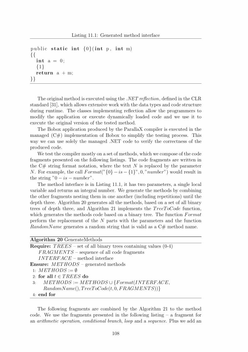
Listing 11.1: Generated method interface

pub l i c stat ic int {0}( int p , int m){{

int a = 0 ;{1}return a + m;

}}

The original method is executed using the .NET reflection, defined in the CLRstandard [31], which allows extensive work with the data types and code structureduring runtime. The classes implementing reflection allow the programmers tomodify the application or execute dynamically loaded code and we use it toexecute the original version of the tested method.

The Bobox application produced by the ParallaX compiler is executed in themanaged (C#) implementation of Bobox to simplify the testing process. Thisway we can use solely the managed .NET code to verify the correctness of theproduced code.

We test the compiler mostly on a set of methods, which we compose of the codefragments presented on the following listings. The code fragments are written inthe C# string format notation, where the text N is replaced by the parameterN . For example, the call Format(”{0}− is−{1}”, 0, ”number”) would result inthe string ”0− is− number”.

The method interface is in Listing 11.1, it has two parameters, a single localvariable and returns an integral number. We generate the methods by combiningthe other fragments nesting them in one another (including repetitions) until thedepth three. Algorithm 20 generates all the methods, based on a set of all binarytrees of depth three, and Algorithm 21 implements the TreeToCode function,which generates the methods code based on a binary tree. The function Formatperform the replacement of the N parts with the parameters and the functionRandomName generates a random string that is valid as a C# method name.

Algorithm 20 GenerateMethods

Require: TREES – set of all binary trees containing values (0-4)FRAGMENTS – sequence of all code fragmentsINTERFACE – method interface

Ensure: METHODS – generated methods1: METHODS := ∅2: for all t ∈ TREES do3: METHODS := METHODS ∪ {Format(INTERFACE,

RandomName(), T reeToCode(t, 0, FRAGMENTS))}4: end for

The following fragments are combined by the Algorithm 21 to the methodcode. We use the fragments presented in the following listing – a fragment foran arithmetic operation, conditional branch, loop and a sequence. Plus we add an

108

Algorithm 21 TreeToCode

Require: TREE – binary tree containing values (0-4), represented in an arrayN – index in the tree, initially 0FRAGMENTS – sequence of all code fragments

Ensure: CODE – generated code1: if N < TREE.Length then2: CODE := Format(FRAGMENTS[N ],

T reeToCode(TREE, 2 ∗N + 1, FRAGMENTS),T reeToCode(TREE, 2 ∗N + 2, FRAGMENTS))

3: else4: CODE := ””5: end if

Listing 11.2: Arithmetic operation

a ∗= p ;

empty string representing empty code, which is used to terminate the replacementat the appropriate depth (three).

Using the presented algorithm and code fragments, we are able to generate ahuge number of methods with all possible nesting of control flow constructs upto the depth of three. We generate nested loops, branches and any combination.The decremental behavior in loops is necessary to prevent endless iteration andassure that the code always ends and produces a valid result.

The correctness test is implemented in the ParallaX project automatic MSUnit test named – CILParserMultitest, distributed along with the project.The description of the project structure and instructions involving the automatictests are in the chapter Attachments: Digital Content.

11.2 Levenshtein Distance Experiments

In this section, we evaluate the performance of the application produced by ourcompiler. We take the blocked implementation of the Wagner–Fischer dynamicprogramming algorithm [91], as explained in Section 10.3. We parallelize theblocked algorithm using the compiler and compare the performance of the result-ing application with the original C# implementation, executed in .NET 4.6 withall optimizations. The blocked version of the algorithm enables the compiler to

Listing 11.3: Conditional branch

i f ( a % 2 == 0){{{0}

}}

109

Listing 11.4: Loop

do {{{0}a += p−−;

}}while (p > 0 ) ;

Listing 11.5: Construct sequence

{0}{1}

optimize the block code and employ vectorization as described in Section 10.4.2.

The compiler produces an application for the native implementation of Bobox.We compare two versions, one is accelerated using the older SSE streaming ex-tension and the other uses the AVX extension. We measure both versions toprovide better insight into the vectorization impact on the overall performanceof the application.

We measure the performance of both the versions on pairs of strings of thesame size varying between 8 and 128 MB. We also measure the performancefor different block sizes, because the block size influences the ratio between thekernel parallelism and vectorization. Bigger blocks provide more opportunities forvectorization, because the blocks inner loop is strongly optimized, where smallerblocks leave more room for parallel computation of separate blocks. We use blockswith height equal to the vector size (4 for SSE and 8 for AVX) and with is alwaysspecified in the experiment.

We measure the performance on two separate systems. First we a serverrunning Windows 10 equipped with the Intel Xeon E5-4620v4 processor, with10 physical cores and 20 virtual threads, and 16 GB of DDR4 random accessmemory. The second platform is a workstation running Windows 10 with Inteli7-6500U CPU, with 2 physical cores and virtual threads, and 8 GB of RAM.We use the high precision Performance counter, available in Windows, which iscapable to measure the time in nanoseconds.

We measure only the actual computation run time, all data is loaded prior tothe application start. In every experiment, we measure the application 10 timesfor both the original and the compiled version and we print the results in a singlebox plot to compare the performance including any special cases.

The experiment results are displayed as the time consumed to complete anelementary task, for Levenshtein distance, this means the computation of thevalue of a single element of the matrix. The results are acquired by dividing thetotal wall time by the size of the matrix. The results are summed in two-quartileboxplots with whiskers signifying the lowest value within 1.5∗ IQR (interquartilerange) of the lower quartile, and the highest value within 1.5 ∗ IQR of the upperquartile. The plots vertical axes are in logarithmic scale.

110

4 4 8 8 16 16

34

56

8

Data size (MB)

Tim

e pe

r el

emen

tary

task

(ns

),lo

g sc

ale

original bobox

4 4 8 8 16 16

23

45

Data size (MB)

Tim

e pe

r el

emen

tary

task

(ns

),lo

g sc

ale

original bobox

Figure 11.1: Levenshtein distance calculated with block size 16, workstation(left)server(right) , Bobox application is accelerated with SSE

2 2 4 4 8 8

23

45

6

Data size (MB)

Tim

e pe

r el

emen

tary

task

(ns

),lo

g sc

ale

original bobox

2 2 4 4 8 8

12

34

Data size (MB)

Tim

e pe

r el

emen

tary

task

(ns

),lo

g sc

ale

original bobox

Figure 11.2: Levenshtein distance calculated with block size 128, workstation(left)server(right) , Bobox application is accelerated with SSE

16 16 32 32 64 64

23

45

6

Data size (MB)

Tim

e pe

r el

emen

tary

task

(ns

),lo

g sc

ale

original bobox

16 16 32 32 64 64

0.5

1.0

2.0

5.0

Data size (MB)

Tim

e pe

r el

emen

tary

task

(ns

),lo

g sc

ale

original bobox

Figure 11.3: Levenshtein distance calculated with block size 1024, worksta-tion(left) server(right) , Bobox application is accelerated with SSE

Figures 11.1, 11.2, 11.3, 11.4 contain the results for the Bobox applicationaccelerated with SSE, where we measure the performance for the block sizes 16,128, 1024 and 32768. The block size defines the width of the parallelogram blocksexplained in the previous chapter, the block height is always equal to the vectorsize (4 for SSE and 8 for AVX).

Figures 11.5, 11.6, 11.7, 11.8 contain the results for the Bobox applicationaccelerated with AVX. The results are better than the SSE acceleration, becauseAVX supports bigger vectors and provides better performance, especially for big-ger blocks.

The compiler is able to apply all the optimization described in Section 7 and

111

16 16 32 32 64 64

23

45

6

Data size (MB)

Tim

e pe

r el

emen

tary

task

(ns

),lo

g sc

ale

original bobox

16 16 32 32 64 64

0.5

1.0

2.0

5.0

Data size (MB)

Tim

e pe

r el

emen

tary

task

(ns

),lo

g sc

ale

original bobox

Figure 11.4: Levenshtein distance calculated with block size 32768, worksta-tion(left) server(right) , Bobox application is accelerated with SSE

4 4 8 8 16 16

46

810

Data size (MB)

Tim

e pe

r el

emen

tary

task

(ns

),lo

g sc

ale

original bobox

4 4 8 8 16 16

23

45

Data size (MB)

Tim

e pe

r el

emen

tary

task

(ns

),lo

g sc

ale

original bobox

Figure 11.5: Levenshtein distance calculated with block size 16, workstation(left)server(right) , Bobox application is accelerated with AVX

2 2 4 4 8 8

23

45

67

Data size (MB)

Tim

e pe

r el

emen

tary

task

(ns

),lo

g sc

ale

original bobox

2 2 4 4 8 8

12

34

Data size (MB)

Tim

e pe

r el

emen

tary

task

(ns

),lo

g sc

ale

original bobox

Figure 11.6: Levenshtein distance calculated with block size 128, workstation(left)server(right) , Bobox application is accelerated with AVX

the special optimization added in Section 10.4. The produced application was ableto employ both vectorization and kernel parallelism thanks to the optimizationswhich significantly reduced the HFG complexity and granularity.

The performance is better for bigger blocks, which provide more opportunitiesfor vectorization and reduced loop overhead. The Bobox application outperformsthe original implementation in all experiments, with the exception of the smallestblock size on the workstation, where the small number of cores and block sizelimit parallelization.

112

16 16 32 32 64 64

23

45

7

Data size (MB)

Tim

e pe

r el

emen

tary

task

(ns

),lo

g sc

ale

original bobox

16 16 32 32 64 64

0.5

1.0

2.0

5.0

Data size (MB)

Tim

e pe

r el

emen

tary

task

(ns

),lo

g sc

ale

original bobox

Figure 11.7: Levenshtein distance calculated with block size 1024, worksta-tion(left) server(right) , Bobox application is accelerated with AVX

16 16 32 32 64 64

23

45

6

Data size (MB)

Tim

e pe

r el

emen

tary

task

(ns

),lo

g sc

ale

original bobox

16 16 32 32 64 64

0.5

1.0

2.0

5.0

Data size (MB)

Tim

e pe

r el

emen

tary

task

(ns

),lo

g sc

ale

original bobox

Figure 11.8: Levenshtein distance calculated with block size 32768, worksta-tion(left) server(right) , Bobox application is accelerated with AVX

11.3 Streaming Experiments

In this section, we evaluate the ParallaX performance for a series of one dimen-sional algorithms. We present a convolution from the DSP category, with datadependences similar to the Levenshtein distance, but in one dimension. Next,we present an algorithm similar to the S-boxes used in the Serpent cipher, withmultiple inputs and outputs. We conclude the experiments with a series of verysimple algorithms, that apply a single function to a stream of value, to test theParallaX compiler on very simple applications.

The experimental environment is the same as in case of the Levenshtein dis-tance. We measure the performance on two separate systems. First, we use aserver, running Windows 10, equipped with the Intel Xeon E5-4620v4 processor,with 10 physical cores and 20 virtual threads, and 16 GB of DDR4 random accessmemory. The second platform is a workstation running Windows 10 with Inteli7-6500U CPU, with 2 physical cores and virtual threads, and 8 GB of RAM.We use the high precision Performance counter, available in Windows, which iscapable to measure the time in nanoseconds.

We measure only the actual computation run time, all data is loaded prior tothe application start. In every experiment, we measure the application 10 timesfor both the original and the compiled version and we print the results in a singlebox plot to compare the performance including any special cases.

The experiment results are displayed as the time consumed to complete anelementary task, for Levenshtein distance, this means the computation of the

113

value of a single element of the matrix. The results are acquired by dividing thetotal wall time by the size of the matrix. The results are summed in two-quartileboxplots with whiskers signifying the lowest value within 1.5∗ IQR (interquartilerange) of the lower quartile, and the highest value within 1.5 ∗ IQR of the upperquartile. The plots vertical axes are in logarithmic scale.

11.3.1 Convolution Experiment

The first experiment is a simple convolution algorithm, which represents simpleralgorithms from the digital signal processing category. The algorithm constructsa new signal by combining the neighboring values of the input signal, using thefunction:

A[I] = 2 ∗B[I]− 0.5 ∗B[I − 1] + 0.5 ∗B[I − 2]

The function contains data dependences between the accesses to the array A,but the dependences are of the type read-read, which do no prevent paralleliza-tion. The application code is in Listing 11.6.

Listing 11.6: Convolution algorithm code

int [ ] Convolution ( int [ ] a , int [ ] b ){

int i = 2 ;int l en = a . Length ;do{

var p r e l a s t = b [ i − 2 ] ;var l a s t = b [ i − 1 ] ;var cur rent = b [ i ] ;a [ i ] = 2 ∗ cur r ent − 0 .5 ∗ l a s t + 0 .5 ∗ p r e l a s t ;i ++;

} while ( i < l en ) ;return a ;

}

The experiment results shown in Figures 11.9 and 11.10. The ParallaX compil-er successfully transformed, optimized and vectorized the code and the resultingapplication outperforms the original C# implementation on both platforms.

11.3.2 Cryptography Experiment

The second experiment is based on the linear transformation used in the SerpentCipher to mix the outputs of the S-Boxes, the boxes combine the data with partsof the key and the transformation produces the final cypher [98]. The algorithmhas four inputs and outputs and combines the values according to the followingequations, where ⊕ denotes xor, <<< denotes left rotation and << denotes leftshift:

114

16 16 32 32 64 64

45

67

89

Data size (MB)

Tim

e pe

r el

emen

tary

task

(ns

),lo

g sc

ale

original bobox

16 16 32 32 64 64

12

5

Data size (MB)

Tim

e pe

r el

emen

tary

task

(ns

),lo

g sc

ale

original bobox

Figure 11.9: Convolution algorithm performance, workstation(left) server(right), Bobox application is accelerated with SSE

16 16 32 32 64 64

34

56

8

Data size (MB)

Tim

e pe

r el

emen

tary

task

(ns

),lo

g sc

ale

original bobox

16 16 32 32 64 64

0.5

1.0

2.0

5.0

Data size (MB)

Tim

e pe

r el

emen

tary

task

(ns

),lo

g sc

ale

original bobox

Figure 11.10: Convolution algorithm performance, workstation(left) server(right), Bobox application is accelerated with AVX

b0 = b0 <<< 13;

b2 = b2 <<< 3;

b1 = b1 ⊕ b0 ⊕ b2;b3 = b3 ⊕ b2 ⊕ (b0 << 3);

b1 = b1 <<< 1;

b3 = b3 <<< 7;

b0 = b0 ⊕ b1 ⊕ b3;b2 = b2 ⊕ b3 ⊕ (b1 << 7);

b0 = b0 <<< 5;

b2 = b2 <<< 22;

The C# implementation of the algorithms is in Listing 11.7. The originalcipher was designed for parallelization and the ParallaX compiler is able to fullyexploit the available parallelism. The experiment results are summed in Fig-ures 11.11 and 11.12, the algorithm is more complex than the convolution ex-periment, because it contains more arithmetic operations that take more time toevaluate.

Listing 11.7: Convolution algorithm code

115

void Cipher ( int [ ] a0 , int [ ] a1 , int [ ] a2 , int [ ] a3 ,int [ ] b0 , int [ ] b1 , int [ ] b2 , int [ ] b3 )

{int i = 0 ;int l en = a0 . Length ;do{

var b 0 = b0 [ i ] ;var b 1 = b1 [ i ] ;var b 2 = b2 [ i ] ;var b 3 = b3 [ i ] ;b 0 = ( b 0 << 13) | ( b 0 >> −13);b 2 = ( b 2 << 3) | ( b 2 >> −3);b 1 = b 1 ˆ b 0 ˆ b 2 ;b 3 = b 3 ˆ b 2 ˆ ( b 0 << 3 ) ;b 1 = ( b 1 << 1) | ( b 1 >> −1);b 3 = ( b 3 << 7) | ( b 3 >> −7);b 0 = b 0 ˆ b 1 ˆ b 3 ;b 2 = b 2 ˆ b 3 ˆ ( b 1 << 7 ) ;b 0 = ( b 0 << 5) | ( b 0 >> −5);b 2 = ( b 2 << 22) | ( b 2 >> −22);a0 [ i ] = b 0 ;a1 [ i ] = b 1 ;a2 [ i ] = b 2 ;a3 [ i ] = b 3 ;i ++;

} while ( i < l en ) ;}

16 16 32 32 64 64

1015

20

Data size (MB)

Tim

e pe

r el

emen

tary

task

(ns

),lo

g sc

ale

original bobox

16 16 32 32 64 64

25

1020

Data size (MB)

Tim

e pe

r el

emen

tary

task

(ns

),lo

g sc

ale

original bobox

Figure 11.11: Serpent linear transformation algorithm performance, worksta-tion(left) server(right) , Bobox application is accelerated with SSE

11.3.3 Baseline Experiments

To evaluate the performance of the applications produced by the ParallaX compil-er for extremely simple applications, we constructed a series of filter-like applica-tions with different structure to examine the application performance in different

116

16 16 32 32 64 64

510

1520

Data size (MB)

Tim

e pe

r el

emen

tary

task

(ns

),lo

g sc

ale

original bobox

16 16 32 32 64 64

12

510

20

Data size (MB)

Tim

e pe

r el

emen

tary

task

(ns

),lo

g sc

ale

original bobox

Figure 11.12: Serpent linear transformation algorithm performance, worksta-tion(left) server(right) , Bobox application is accelerated with AVX

situations. We use the function Filter defined in Listing 11.8 to process the val-ues and we use them in varying control flow structures to test the performance.The functions are purely artificial, designed to provide the required computation-al complexity and neither compiler uses the common sub-expressions to optimizethe application (we verified it by studying both the HFG and the CIL producedby C# compiler).

Listing 11.8: Filter code

int F i l t e r ( int [ ] b , int i ){

int x = b [ i ] + i∗ i ∗ i ∗ i ∗ i ∗ i ∗ i∗ i ∗ i ∗ i ∗ i ∗ i ∗ i∗ i ∗ i ∗ i ∗ i ∗ i ∗ i∗ i ∗ i ∗ i ∗ i ∗ i ∗ i ;

return i ∗ x ;}

11.3.4 Single Filter

The first application applies the Filter function to a series of values in a sin-gle loop, Listing 11.9 contains the application code. The performance of theapplication is shown in Figure 11.13.

Listing 11.9: Complex filter code

int [ ] S i n g l e F i l t e r ( int [ ] a , int [ ] b ){

int i = 0 ;do{

a [ i ] = F i l t e r (b , i ) ;i ++;

} while ( i < a . Length ) ;

117

return a ;}

16 16 32 32 64 64

24

68

Data size (MB)

Tim

e pe

r el

emen

tary

task

(ns

),lo

g sc

ale

original bobox

16 16 32 32 64 64

0.5

1.0

2.0

5.0

Data size (MB)

Tim

e pe

r el

emen

tary

task

(ns

),lo

g sc

ale

original bobox

Figure 11.13: Performance of the SingleF ilter application, workstation(left)server(right) , Bobox application is accelerated with AVX

11.3.5 Serial Filter

The second application applies two filters to a series of data in two loops, one afteranother. Listing 11.10 contains the application code, where the Filter function iseither the SimpleF ilter or ComplexF ilter. The performance of the applicationis shown in Figure 11.14.

Listing 11.10: Complex filter code

int [ ] S e r i a l F i l t e r ( int [ ] a , int [ ] b , int [ ] c ){

// f i l t e r 1int i = 0 ;do{

a [ i ] = F i l t e r (b , i ) ;i ++;

} while ( i < a . Length ) ;

// f i l t e r 2i = 0 ;do{

c [ i ] = F i l t e r ( a , i ) ;i ++;

} while ( i < c . Length ) ;

return c ;}

118

16 16 32 32 64 64

510

15

Data size (MB)

Tim

e pe

r el

emen

tary

task

(ns

),lo

g sc

ale

original bobox

16 16 32 32 64 64

12

510

Data size (MB)

Tim

e pe

r el

emen

tary

task

(ns

),lo

g sc

ale

original bobox

Figure 11.14: Performance of the SerialF ilter application, workstation(left) serv-er(right) , Bobox application is accelerated with AVX

11.3.6 Multiple Filter

The last application applies two filters in parallel and then it merges the resultin three loops. Listing 11.11 contains the application code, where the Filterfunction is either the SimpleF ilter or ComplexF ilter. The performance of theapplication is shown in Figure 11.15.

Listing 11.11: Multi filter code

int [ ] M u l t i F i l t e r ( int [ ] a , int [ ] b , int [ ] c , int [ ] d ){

// f i l t e r 1int i = 0 ;do{

b [ i ] = F i l t e r ( a , i ) ;i ++;

} while ( i < a . Length ) ;

// f i l t e r 2int i = 0 ;do{

d [ i ] = F i l t e r ( c , i ) ;i ++;

} while ( i < c . Length ) ;

// mergeint i = 0 ;do{

a [ i ] = b [ i ] + d [ i ] ;i ++;

} while ( i < a . Length ) ;return a ;

}

119

16 16 32 32 64 64

510

1520

Data size (MB)

Tim

e pe

r el

emen

tary

task

(ns

),lo

g sc

ale

original bobox

16 16 32 32 64 64

12

510

20

Data size (MB)

Tim

e pe

r el

emen

tary

task

(ns

),lo

g sc

ale

original bobox

Figure 11.15: Performance of the MultiF ilter application, workstation(left) serv-er(right) , Bobox application is accelerated with AVX

11.3.7 Experiment Conclusions

The results show that the currently produced Bobox plans are efficient enoughthat the final Bobox applications outperform the original C# implementation.The results are better for applications that contain more arithmetic operationsthan control flow, especially for bigger data sets. This means that the morecalculations outweigh control flow, the better is the Bobox doing in comparisonto the original application.

The results are best for the more complex applications accelerated with theAVX extension. The produced Bobox applications achieve speedup roughly equalto the number of cores of the CPU. The achieved performance is not ideal, but theresults suggest that the approach is viable. Additional optimizations can furtherimprove the performance of the final applications.

120

12. Conclusions

We introduce the Hybrid Flow Graph as an alternative intermediate represen-tation for procedural code. The main advantage of the HFG is its conceptualequivalence to streaming systems which, consequently, allows the use of stream-ing systems as run-time environments for such programs. HFG can be used acrossmultiple systems, because it does not contain any domain-specific concepts.

We successfully implemented a prototype compiler that allows programmersto design simple streaming applications in a restricted version of the C# languageand transform the produced code into HFG which is then executed in the Boboxstreaming system.

The compiler supports code written in a restricted version of the C# language,where we limit the use of concepts that significantly modify control flow, like ex-ception management. We experimentally verified the correctness of the producedapplications on a huge collection of generated methods, which we transformed,executed and compared the results with the original.

Although the HFG allows direct execution by a streaming system, it requiresadvanced optimizations to produce efficient applications. As our measurementspresented in Section 11 show, these steps reduce the synchronization overhead sosignificantly that the performance bonuses, associated with vectorized executionavailable in streaming systems, become clearly visible. The produced applicationsdo not use the system resources to the maximal extent, but additional optimiza-tions should further improve the performance.

In our experiment setup, we were able to produce plans for the Bobox stream-ing environment that outperform the original C# code. These result suggest thattransforming a well-known procedural language to streaming plans is a viable al-ternative to dedicated non-procedural streaming languages. This approach allowsthe use of streaming systems by programmers who are not experts in C++ and/orparallel programming.

The steps used to optimize the code used for our experiments (Section 11) areonly a part of the effort required to encompass the variability of programmingpatterns which must be supported by any parallelizing or vectorizing technique.Thus, our current and future work will focus on further optimizing steps – severaltraditional compiler techniques such as loop skewing may be transferred to theenvironment of HFG; however, there are also optimization techniques native tothe streaming environments that we would like to introduce to our system.

The compiler is currently able to handle all aliases in the code, because werestrict reference data types in the input code, with the exception of arrays.Arrays can cause aliasing between subscripts, but we handle the arrays as compactobjects, which prevents aliasing at the expense of efficiency. This behavior ischanged by optimizations that break arrays into streams and access the elementsone by one, but the optimizations are designed to be applicable only when thereis no risk of aliasing.

121

12.1 Future Work

In our future work, we will focus on widening the scope of applications the Paral-laX compiler is able to transform and optimize efficiently. We will remove someof the restrictions currently imposed on the supported source code and we willfurther improve the code generation process to allow the compiler to producebuilding blocks of the Bobox applications to encompass the use cases presentedin the motivation.

We currently use method integration (inlining) to process method calls, but itis also possible to use the layered HFG to perform inter-procedural analysis. Wecan introduce more layers to represent the called methods and their components,thus creating basically a graph of Hybrid Flow Graphs. This way, the compilerwill be able to handle a wider scope of applications, including recursion.

The structure of streaming applications does not allow for a full object modelsupported by C#. We will add at least structs, because they do not have referencesemantics and thus do not introduce complex aliasing. A full object support isnot necessary, because the compiler was not designed to optimize general C#applications, but as a tool to implement algorithmic parts of bigger streamingapplications, such as database-like queries. These applications require at leastarrays, but the introduction of structures could simplify their design.

We can treat the structures as arrays and always transfer and access theentire structure at once, or we might be able to break the structures into separatevariables and handle them more efficiently. The second approach means that wetreat a.x, a.y, b.x and b.y as separate variables for V ector2 a, b. This approach ismore efficient, but it requires more complex analysis to prevent aliasing, especiallywhen the method integration introduces multiple structure variables.

Our current experiments focus mainly on data intensive applications as ourtarget use cases, which are mostly streaming processing friendly. Other appli-cations are also supported by the compiler, but their performance is inferior,because they would require other special optimizations which are not currentlyimplemented. In the future we will focus on additional optimizations necessaryto produce efficient code for a wider selection of application.

In this work, we present a compiler that allows programmers to design stream-ing applications with the C# programming language. Our work was motivatedby the intention to design algorithmic parts of bigger streaming applications ina general programming language and integrate them directly into the streamingapplication. To achieve this goal, the compiler must be able to produce partsof streaming applications and integrate them with existing plans. This processis not yet implemented, but it requires only a minor modification of the inputsand outputs, which must be properly connected to the wider plan and we willimplement the changes in our future work.

122

Appendix A: CompilerInfrastructure

The ParallaX compiler for streaming environments presented in this work is acomplex piece of software, which requires configuration to provide access to allits features. This sections provides information about the configuration, generalwork-flow and examples of an application structure that takes advantage of thecompiler features.

The compiler internally uses a newly developed intermediate language calledHybrid flow graph or HFG to represent the parallelized code. Each processedapplication is transformed to HFG, the resulting code can be used to parallelizeapplications or it can be exported directly and executed by external parallelenvironment, like Bobox. This allows us to process an application, produce a setof HFG algorithms that we can combine directly in a streaming environment. Thecompiler can be used as a cross-compiler for parallel environments that requireinput in a form of computation plan represented by a directed graph, like Bobox.

12.2 Compiler Work Flow

The compiler is presented in detail in Chapters 5, 6, 7 and 8. It provides a unifiedinterface, based on C# code, and it offers multiple target platforms, focusingmostly on the Bobox system. The work-flow is strongly influenced by the targetplatforms, because they introduce additional steps and requirements.

The main target platform is the native implementation of the Bobox streamingenvironment. The overview of its work flow is in Figure 12.1, where the compilerproduces execution plan and kernels for Bobox and the user must integrate thecomponents with the environment. In the case of a managed Bobox, this can bedone dynamically by attaching Bobox as a library, but the native (C++) imple-mentation must be compiled along with the custom kernels to achieve optimalperformance. This allows the C++ compiler to optimize the kernels along withthe rest of the code.

C# code

C#

compiler

CIL codeParallaX

compilerkernels

Bobox

application

plan Bobox

Figure 12.1: ParallaX compiler architecture

Our compiler also provides back-end for direct parallelization of C# applica-tions, either by integrating the managed implementation of Bobox or by trans-forming the application code into asynchronous methods. The work-flow for both

123

platforms is very similar and requires much less additional work on the side of theprogrammer. The compiler simply produces a new .NET application that withdifferent code but the same behavior. This work-flow is summed in Figure 12.2,where the Bobox runtime and execution plans are necessary only for the Boboxintegration method.

C# code

C#

compiler

CIL codeParallaX

compiler

Bobox

runtime

modified

CIL

execution

plans

optimized

application

Boboxintegration

Figure 12.2: Compiler work flow overview

Both the different work-flows require that the input application is implement-ed in C#, compiled into CIL and then fed to our compiler. This extra step canbe automatized via scripts or pre-build code.

12.3 Application structure

The compiler provides the user with a complete control over the applicationprocessing and parallelization, because parallelism is beneficial only for certainalgorithms. The optimization process is controlled by two factors - the applicationstructure and the compiler configuration. The configuration is explained in nextsection.

An application, that is to be parallelized, can be annotated by special at-tributes provided as part of a tiny library distributed with the compiler. Theseattributes do not modify the application behavior in any way, they are just usedby the compiler to locate parts of code that should be parallelized or transformedto plan and kernels.

The code in Listing 12.1 shows a simple application that adds numbers in aloop. The Add method has an attribute called Transform that tells the compilerwhat is to be done with the function. The attribute has a parameter that specifiesthe operation performed by the compiler. Each operation is identified by a stringand it is applied to all methods or classes that have the Transform attribute withthat exact string as parameter.

The actual operations are defined the compiler configuration described innext section. The configuration defines the operation identifiers which are thencompared to the parameters of the Transform attributes used in the application.

The Add method is very simple and it would have been integrated by the.NET JIT compiler, but by transforming it to a HFG, we can make it run inparallel for each iteration of the loop. This does not improves performance as themethod is too simple, but it serves as an example.

124

Listing 12.1: Annotated application

class Program{

[ Transform ( ” CreateBobolang ” ) ]stat ic int Add( int A, int B){

return A + B;}

stat ic void Main( s t r i n g [ ] a rgs ){

for ( int i = 0 ; i < 1000 ; i++){

int r e s += Add( i , 1 00 ) ;}Console . WriteLine ( r e s ) ;

}}

12.4 Compiler Configuration

The compiler work is controlled by a XML configuration file. The configurationcontains a list of transformation files, where each transformation file represents aset of transformations applied to a single assembly and its result is exported asa new assembly. The transformation files are applied in series, which allows forrecursive optimizations.

A transformation file contains a list of profiles, where each profile representsa single transformation applied to all methods with the attribute Transform,where the profiles name matches the attributes parameter profile name. Fig-ure 12.3 contains a schematic view on the application configuration in an UML-like notation.

ConfigurationTransformation

file

Profile[name]

*

*

ParallaX

Input

assembly

Method[Transform(name)]

*

*

1

1

Figure 12.3: Configuration file structure

12.4.1 Configuration File

The configuration also contains parameter OptimizationLevelLogging that de-fines how much information is logged during the optimization. Available values

125

Listing 12.2: Compiler configuration file

<?xml version=” 1 .0 ”?><Globa lConf igurat ion><Transf i leNames><s t r i n g> t r a n s f i l e . xml</ s t r i n g>

</ Transf i leNames><Optimizeat ionLoggingLeve l>None</ Optimizeat ionLoggingLeve l>

</ Globa lConf igurat ion>

are None, Info and Debug, where None prints no logs (only fatal errors) andDebug outputs everything. Listing 12.2 shows a sample configuration file.

12.4.2 Transformation File

Transformation files have two parameters TargetAssembly and OutputAssembly,which identify input and output assemblies. The transformation files can bechained to incrementally modify an assembly, because every transformation fileproduces a new version that can be loaded by the following transformation file.

All transformation files and profiles are processed in the order they are defined.The profiles always apply only to the methods with the attribute Transform withthe profiles name as parameter. Each transformation file loads a single assembly,processes all the profiles and produces a new assembly.

Listing 12.3 shows a simple transformation file, which contains a profile namedCreateBobolang. The C# source code shown in Listing 12.1 would be affectedby this configuration, because the Add method has an attribute Transform witha parameter ”CreateBobolang”. This particular transformation file contains asingle profile that represents the CreateBobolang optimization, which produces aBobox execution plan from every method with the proper Transform attribute.

126

Listing 12.3: Compiler transformation file

<?xml version=” 1 .0 ”?><T r a n s f i l e><TargetAssembly>Example . exe<TargetAssembly><OutputAssembly>Example out . exe<OutputAssembly><P r o f i l e s>

<P r o f i l e><Name>CreateBobolang</Name><Pro f i l eOpt im i za t i on>

CreateBobolang</ Pro f i l eOpt im i za t i on><Optimizat ionParameters><s t r i n g>bobolang1 . txt</ s t r i n g>

</ OptimizationParameters></ P r o f i l e>

</ P r o f i l e s></ T r a n s f i l e>

127

128

Appendix A: Compiler Library

This chapter is focuses on the library distributed along with the ParallaX com-piler. The library, called ParallaXMath, is part of the ParallaX interface thatprovides the attributes used to control the compiler process, see Appendix A fordetails.

The library is designed as an analogy of the Math library distributed as partof the .NET framework, we include most of the same functions, like minimum(min) or absolute value (abs). The library provides fully functioning proceduresthat can be tested with the C# source code.

The library functions are recognized by the ParallaX compiler, which does notintegrate them. Instead, the compiler transforms each call to one of the functionsdirectly into an optimized custom node that implements its functionality. Thisgives programmers the basic arithmetic functionality and also allows them toproduce more efficient code, because the compiler can use specifically optimizednodes, instead of using general optimizations.

The library currently provides only a limited selection of functions, becauseit is a prototype designed to support the tests and experiments presented in thiswork. The final release will contain more functions and algorithms to providea good foundation for the applications designed for the compiler. The librarycurrently provides the following functions:

• Min – minimum of two numbers.

• Max – maximum of two numbers.

• Abs – absolute value of a number.

• Sign – sign of a signed integral number.

• Equals – compares two values for equality and converts the result to integer.

• NotEquals – negation of Equals.

129

130

Bibliography

[1] Michal Brabec and David Bednarek. Programming parallel pipelines usingnon-parallel C# code. CEUR Workshop Proceedings, 1003:82–87, 2013.

[2] Zbynek Falt, Martin Krulis, David Bednarek, Jakub Yaghob, and Filip Za-voral. Locality aware task scheduling in parallel data stream processing. InDavid Camacho, Lars Braubach, Salvatore Venticinque, and Costin Badi-ca, editors, Intelligent Distributed Computing VIII, volume 570 of Studies inComputational Intelligence, pages 331–342. Springer International Publish-ing, 2015.

[3] Zbynek Falt, David Bednarek, Martin Krulis, Jakub Yaghob, and Filip Zavo-ral. Bobolang: A language for parallel streaming applications. In Proceedingsof the 23rd international symposium on High-performance parallel and dis-tributed computing, pages 311–314. ACM, 2014.

[4] Ian Buck, Tim Foley, Daniel Horn, Jeremy Sugerman, Kayvon Fatahalian,Mike Houston, and Pat Hanrahan. Brook for GPUs: stream computing ongraphics hardware. In ACM Transactions on Graphics (TOG), volume 23,pages 777–786. ACM, 2004.

[5] Frederic Boussinot and Robert De Simone. The ESTEREL language. Pro-ceedings of the IEEE, 79(9):1293–1304, 1991.

[6] Xin Li and Reinhard Von Hanxleden. Multithreaded reactive programming– the Kiel Esterel processor. Computers, IEEE Transactions on, 61(3):337–349, 2012.

[7] William Thies, Michal Karczmarek, and Saman Amarasinghe. StreamIt: Alanguage for streaming applications. In Compiler Construction, pages 179–196. Springer, 2002.

[8] A. Hagiescu, W. F. Wong, D. F. Bacon, and R. Rabbah. A computingorigami: Folding streams in FPGAs. In Design Automation Conference,2009. DAC ’09. 46th ACM/IEEE, pages 282–287, July 2009.

[9] Daniel J. Abadi, Don Carney, Ugur Cetintemel, Mitch Cherniack, Chris-tian Convey, Sangdon Lee, Michael Stonebraker, Nesime Tatbul, and StanZdonik. Aurora: A new model and architecture for data stream management.The VLDB Journal, 12(2):120–139, August 2003.

[10] Arvind Arasu, Brian Babcock, Shivnath Babu, Mayur Datar, Keith Ito,Itaru Nishizawa, Justin Rosenstein, and Jennifer Widom. STREAM: Thestanford stream data manager (demonstration description). In Proceedings ofthe 2003 ACM SIGMOD International Conference on Management of Data,SIGMOD ’03, pages 665–665, New York, NY, USA, 2003. ACM.

[11] Dhruba Borthakur, Jonathan Gray, Kannan Sarma, Joydeep Sen Spiegel-berg, Nicolas Muthukkaruppan, Hairong Kuang, Karthik Ranganathan,Dmytro Molkov, Aravind Menon, Samuel Rash, et al. Apache hadoop goes

131

realtime at facebook. In Proceedings of the 2011 ACM SIGMOD Interna-tional Conference on Management of data, pages 1071–1080. ACM, 2011.

[12] Hakan Kocakulak and Tugba Taskaya Temizel. A hadoop solution forballistic image analysis and recognition. In High Performance Computingand Simulation (HPCS), 2011 International Conference on, pages 836–842.IEEE, 2011.

[13] Jeffrey Dean and Sanjay Ghemawat. Mapreduce: a flexible data processingtool. Communications of the ACM, 53(1):72–77, 2010.

[14] Milind Bhandarkar. Mapreduce programming with apache hadoop. In Paral-lel & Distributed Processing (IPDPS), 2010 IEEE International Symposiumon, pages 1–1. IEEE, 2010.

[15] Jeffrey Dean and Sanjay Ghemawat. Mapreduce: simplified data processingon large clusters. Communications of the ACM, 51(1):107–113, 2008.

[16] Paul Zikopoulos, Chris Eaton, et al. Understanding big data: Analytics forenterprise class hadoop and streaming data. McGraw-Hill Osborne Media,2011.

[17] Christopher Olston, Benjamin Reed, Utkarsh Srivastava, Ravi Kumar, andAndrew Tomkins. Pig latin: a not-so-foreign language for data processing.In Proceedings of the 2008 ACM SIGMOD international conference on Man-agement of data, pages 1099–1110. ACM, 2008.

[18] Zbynek Falt, David Bednarek, Martin Krulis, Jakub Yaghob, and Filip Zavo-ral. Bobolang: A language for parallel streaming applications. In Proceedingsof the 23rd International Symposium on High-performance Parallel and Dis-tributed Computing, HPDC ’14, pages 311–314, New York, NY, USA, 2014.ACM.

[19] Martin Krulis, David Bednarek, Zbynek Falt, Jakub Yaghob, and Filip Za-voral. Towards semi-automated parallelization of data stream processing. InIntelligent Distributed Computing IX, pages 235–245. Springer, 2016.

[20] Hartmut Ehrig, Grzegorz Rozenberg, and Hans-Jorg Kreowski. Handbook ofgraph grammars and computing by graph transformation, volume 3. worldScientific, 1999.

[21] Reiko Heckel. Graph transformation in a nutshell. Electronic notes in theo-retical computer science, 148(1):187–198, 2006.

[22] Hartmut Ehrig, Michael Pfender, and Hans Jurgen Schneider. Graph-grammars: An algebraic approach. In Switching and Automata Theory,1973. SWAT’08. IEEE Conference Record of 14th Annual Symposium on,pages 167–180. IEEE, 1973.

[23] Michael Lowe. Algebraic approach to single-pushout graph transformation.Theoretical Computer Science, 109(1):181–224, 1993.

132

[24] Hartmut Ehrig, Reiko Heckel, Martin Korff, Michael Lowe, Leila Ribeiro,Annika Wagner, and Andrea Corradini. Algebraic approaches to graph trans-formation: part ii: single pushout approach and comparison with doublepushout approach. In Handbook of Graph Grammars, pages 247–312, 1997.

[25] Gilles Kahn and David MacQueen. Coroutines and networks of parallelprocesses. 1976.

[26] Stephen A Edwards. Kahn process networks. Languages for Digital EmbeddedSystems, pages 189–195, 2000.

[27] Todor Stefanov, Claudiu Zissulescu, Alexandru Turjan, Bart Kienhuis, andEd Deprettere. System design using kahn process networks: the com-paan/laura approach. In Proceedings of the conference on Design, automa-tion and test in Europe-Volume 1, page 10340. IEEE Computer Society,2004.

[28] Edward A Lee and Thomas M Parks. Dataflow process networks. Proceedingsof the IEEE, 83(5):773–801, 1995.

[29] Zeljko Vrba, Pal Halvorsen, Carsten Griwodz, and Paul Beskow. Kahn pro-cess networks are a flexible alternative to mapreduce. In High PerformanceComputing and Communications, 2009. HPCC’09. 11th IEEE InternationalConference on, pages 154–162. IEEE, 2009.

[30] European Computer Manufacturers Association et al. Standard ECMA-334:C# Language Specification. ECMA, 2006.

[31] ECMA ECMA. 335: Common language infrastructure (cli). ECMA, Geneva(CH),, 2005.

[32] David S Platt. Introducing Microsoft. Net. Microsoft press, 2002.

[33] Miguel de Icaza, P MOLARO, R PRATAP, D PORTER, et al. The monoproject. Available from www. mono-project. com, 2004.

[34] Michal Brabec, David Bednarek, and Petr Maly. Transformation of pipelinestage algorithms to event-driven code. In ITAT, pages 13–20, 2014.

[35] Steven S. Muchnick. Advanced compiler design implementation. MorganKaufmann Publishers, 1997.

[36] Randy Allen and Ken Kennedy. Optimizing compilers for modern architec-tures. Morgan Kaufmann San Francisco, 2002.

[37] Michal Brabec and David Bednarek. Transforming procedural code forstreaming environments. In Parallel, Distributed and Network-based Pro-cessing (PDP), 2017 25th Euromicro International Conference on, pages167–175. IEEE, 2017.

[38] Michal Brabec and David Bednarek. Procedural code representation in aflow graph. In DATESO, pages 89–100, 2015.

133

[39] James L. Peterson. Petri nets. ACM Comput. Surv., 9(3):223–252, Septem-ber 1977.

[40] KAHN Gilles. The semantics of a simple language for parallel programming.In Information Processing: Proceedings of the IFIP Congress, volume 74,pages 471–475, 1974.

[41] Mark B Josephs. Models for data-flow sequential processes. In Commu-nicating Sequential Processes. The First 25 Years, pages 85–97. Springer,2005.

[42] Joaquin Ezpeleta, Jose Manuel Colom, and Javier Martinez. A Petrinet based deadlock prevention policy for flexible manufacturing systems.Robotics and Automation, IEEE Transactions on, 11(2):173–184, 1995.

[43] Marc Geilen and Twan Basten. Requirements on the execution of Kahnprocess networks. In Programming languages and systems, pages 319–334.Springer, 2003.

[44] Angeles Navarro, Rafael Asenjo, Siham Tabik, and Calin Cascaval. Analyt-ical modeling of pipeline parallelism. In Parallel Architectures and Compi-lation Techniques, 2009. PACT’09. 18th International Conference on, pages281–290. IEEE, 2009.

[45] Zbynek Falt, Miroslav Cermak, Jirı Dokulil, and Filip Zavoral. ParallelSPARQL query processing using Bobox. International Journal On Advancesin Intelligent Systems, 5(3 and 4):302–314, 2012.

[46] Jeanne Ferrante, Karl J Ottenstein, and Joe D Warren. The program depen-dence graph and its use in optimization. ACM Transactions on ProgrammingLanguages and Systems (TOPLAS), 9(3):319–349, 1987.

[47] Leif Geiger and Albert Zundorf. Graph based debugging with fujaba. Electr.Notes Theor. Comput. Sci., 72(2):112, 2002.

[48] Daniel Balasubramanian, Anantha Narayanan, Christopher van Buskirk,and Gabor Karsai. The graph rewriting and transformation language: Great.Electronic Communications of the EASST, 1, 2007.

[49] Hartmut Ehrig, Karsten Ehrig, Ulrike Prange, and Gabriele Taentzer. Graphtransformation systems. Fundamentals of Algebraic Graph Transformation,pages 37–71, 2006.

[50] Andrea Corradini, Fernando Luıs Dotti, Luciana Foss, and Leila Ribeiro.Translating java code to graph transformation systems. In Graph Transfor-mations, pages 383–398. Springer, 2004.

[51] Mark Thompson, Hristo Nikolov, Todor Stefanov, Andy D. Pimentel,Cagkan Erbas, Simon Polstra, and Ed F. Deprettere. A framework forrapid system-level exploration, synthesis, and programming of multimediamp-socs. In Proceedings of the 5th IEEE/ACM International Conference onHardware/Software Codesign and System Synthesis, pages 9–14. ACM, 2007.

134

[52] Manu Sridharan and Rastislav Bodık. Refinement-based context-sensitivepoints-to analysis for Java. ACM SIGPLAN Notices, 41(6):387–400, 2006.

[53] Thomas Reps. Program analysis via graph reachability. Information andsoftware technology, 40(11):701–726, 1998.

[54] Frances E Allen. Control flow analysis. In ACM Sigplan Notices, volume 5,pages 1–19. ACM, 1970.

[55] Michal Brabec, David Bednarek, and Petr Maly. Transformation of pipelinestage algorithms to event-driven code. In Vera Kurkova, Lukas Bajer, andVojtech Svatek, editors, Proceedings of the 14th Conference on InformationTechnologies - Applications and Theory, Jasna, Slovakia, 2014., volume 1214of CEUR Workshop Proceedings, pages 13–20. CEUR-WS.org, 2014.

[56] Michal Brabec and David Bednarek. Programming parallel pipelines usingnon-parallel c# code. In ITAT, pages 82–87, 2013.

[57] Alfred V Aho, Monica S Lam, Ravi Sethi, and Jeffrey D Ullman. Compilers:principles, techniques, & tools, volume 1009. Pearson/Addison Wesley, 2007.

[58] Krste Asanovic, Stephen W. Keckler, Yunsup Lee, Ronny Krashinsky, andVinod Grover. Convergence and scalarization for data-parallel architectures.In Proceedings of the 2013 IEEE/ACM International Symposium on CodeGeneration and Optimization (CGO), CGO ’13, pages 1–11, Washington,DC, USA, 2013. IEEE Computer Society.

[59] S. A. Edwards. The challenges of synthesizing hardware from C-like lan-guages. IEEE Design Test of Computers, 23(5):375–386, May 2006.

[60] S. J. Allan and A. E. Oldehoeft. A flow analysis procedure for the transla-tion of high-level languages to a data flow language. IEEE Transactions onComputers, C-29(9):826–831, Sept 1980.

[61] P. A. Arras, D. Fuin, E. Jeannot, and S. Thibault. DKPN: A compositedataflow/Kahn process networks execution model. In 2016 24th Euromi-cro International Conference on Parallel, Distributed, and Network-BasedProcessing (PDP), pages 27–34, Feb 2016.

[62] F. Yazdanpanah, C. Alvarez-Martinez, D. Jimenez-Gonzalez, and Y. Etsion.Hybrid dataflow/von-Neumann architectures. IEEE Transactions on Paral-lel and Distributed Systems, 25(6):1489–1509, June 2014.

[63] Marco Danelutto, Tiziano De Matteis, Gabriele Mencagli, and MassimoTorquati. Data stream processing via code annotations. The Journal ofSupercomputing, pages 1–15, 2016.

[64] M. Danelutto, J. D. Garcia, L. M. Sanchez, R. Sotomayor, and M. Torquati.Introducing parallelism by using repara c++11 attributes. In 2016 24thEuromicro International Conference on Parallel, Distributed, and Network-Based Processing (PDP), pages 354–358, Feb 2016.

135

[65] Jiutao Nie, Buqi Cheng, Shisheng Li, Ligang Wang, and Xiao-Feng Li.Vectorization for Java. In Network and Parallel Computing, pages 3–17.Springer, 2010.

[66] Curt Albert, Alastair Murray, and Binoy Ravindran. Applying source levelauto-vectorization to Aparapi Java. In Proceedings of the 2014 InternationalConference on Principles and Practices of Programming on the Java plat-form: Virtual machines, Languages, and Tools, pages 122–132. ACM, 2014.

[67] Alan Leung, Ondrej Lhotak, and Ghulam Lashari. Parallel execution ofJava loops on graphics processing units. Science of Computer Programming,78(5):458–480, 2013.

[68] Rafael Duarte, Alexandre Mota, and Augusto Sampaio. Introducing con-currency in sequential Java via laws. Information Processing Letters,111(3):129–134, 2011.

[69] Walter Cazzola and Edoardo Vacchi. @ java: Bringing a richer annotationmodel to Java. Computer Languages, Systems & Structures, 40(1):2–18,2014.

[70] Cristian Dittamo, Antonio Cisternino, and Marco Danelutto. Parallelizationof C# programs through annotations. In Computational Science–ICCS 2007,pages 585–592. Springer, 2007.

[71] Soumya S Chatterjee and R Gururaj. Lazy-parallel function calls for auto-matic parallelization. In Computational Intelligence and Information Tech-nology, pages 811–816. Springer, 2011.

[72] Yeoul Na, Seon Wook Kim, and Youngsun Han. Javascript parallelizing com-piler for exploiting parallelism from data-parallel html5 applications. ACMTransactions on Architecture and Code Optimization (TACO), 12(4):64,2016.

[73] Martin Krulis. Is there a free lunch for image feature extraction in web appli-cations. In International Conference on Similarity Search and Applications,pages 323–331. Springer, 2015.

[74] Jakub Misek, Benjamin Fistein, and Filip Zavoral. Inferring common lan-guage infrastructure metadata for an ambiguous dynamic language type. InOpen Systems (ICOS), 2016 IEEE Conference on, pages 111–116. IEEE,2016.

[75] Paolo Tonella, Giuliano Antoniol, Roberto Fiutem, and Ettore Merlo.Variable-precision reaching definitions analysis. Journal of Software Main-tenance: Research and Practice, 11(2):117–142, 1999.

[76] Stephen Richardson and Mahadevan Ganapathi. Interprocedural analysis vs.procedure integration. Information Processing Letters, 32(3):137–142, 1989.

[77] George Necula, Scott McPeak, Shree Rahul, and Westley Weimer. Cil: In-termediate language and tools for analysis and transformation of c programs.In Compiler Construction, pages 209–265. Springer, 2002.

136

[78] Herodotos Herodotou and Shivnath Babu. Profiling, what-if analysis, andcost-based optimization of mapreduce programs. Proceedings of the VLDBEndowment, 4(11):1111–1122, 2011.

[79] Jakub Misek and Filip Zavoral. Control flow ambiguous-type inter-procedural semantic analysis for dynamic language compilation. ProcediaComputer Science, 109:955–962, 2017.

[80] Marc Berndl, Ondrej Lhotak, Feng Qian, Laurie Hendren, and Navin-dra Umanee. Points-to analysis using BDDs. ACM SIGPLAN Notices,38(5):103–114, 2003.

[81] Jb Evain. Mono cecil. a vailable at: http://www. mono-p roject. com/Cecil,accessed May, 2007.

[82] Henry G Baker. Garbage collection, tail recursion and first-class continua-tions in stack-oriented languages, December 31 1996. US Patent 5,590,332.

[83] David Bednarek, Michal Brabec, and Martin Krulis. Improving matrix-based dynamic programming on massively parallel accelerators. InformationSystems, 64:175–193, 2017.

[84] Hongwei Xi. Dead code elimination through dependent types. In PADL,volume 99, pages 228–242. Springer, 1999.

[85] David Grove, Greg DeFouw, Jeffrey Dean, and Craig Chambers. Callgraph construction in object-oriented languages. ACM SIGPLAN Notices,32(10):108–124, 1997.

[86] Martin Krulis, David Bednarek, and Michal Brabec. Improving parallel pro-cessing of matrix-based similarity measures on modern gpus. In InternationalConference on Similarity Search and Applications, pages 283–294. Springer,2015.

[87] Meinard Muller. Dynamic time warping. Information retrieval for musicand motion, pages 69–84, 2007.

[88] Doruk Sart, Abdullah Mueen, Walid Najjar, Eamonn Keogh, and Vit Ni-ennattrakul. Accelerating dynamic time warping subsequence search withgpus and fpgas. In Data Mining (ICDM), 2010 IEEE 10th InternationalConference on, pages 1001–1006. IEEE, 2010.

[89] Temple F Smith and Michael S Waterman. Identification of common molec-ular subsequences. Journal of molecular biology, 147(1):195–197, 1981.

[90] Yang Liu, Wayne Huang, John Johnson, and Sheila Vaidya. Gpu accelerat-ed smith-waterman. In Computational Science–ICCS 2006, pages 188–195.Springer, 2006.

[91] Robert A Wagner and Michael J Fischer. The string-to-string correctionproblem. Journal of the ACM (JACM), 21(1):168–173, 1974.

137

[92] Guillermo Delgado and C Aporntewan. Data dependency reduction in dy-namic programming matrix. In Computer Science and Software Engineering(JCSSE), 2011 Eighth International Joint Conference on, pages 234–236.IEEE, 2011.

[93] Ayumu Tomiyama and Reiji Suda. Automatic parameter optimization foredit distance algorithm on gpu. In High Performance Computing for Com-putational Science-VECPAR 2012, pages 420–434. Springer, 2013.

[94] Svetlin A Manavski and Giorgio Valle. Cuda compatible gpu cards as effi-cient hardware accelerators for smith-waterman sequence alignment. BMCbioinformatics, 9(Suppl 2):S10, 2008.

[95] Lukasz Ligowski and Witold Rudnicki. An efficient implementation of smithwaterman algorithm on gpu using cuda, for massively parallel scanning ofsequence databases. In Parallel & Distributed Processing, 2009. IPDPS 2009.IEEE International Symposium on, pages 1–8. IEEE, 2009.

[96] Ali Khajeh-Saeed, Stephen Poole, and J Blair Perot. Acceleration of thesmith–waterman algorithm using single and multiple graphics processors.Journal of Computational Physics, 229(11):4247–4258, 2010.

[97] Yongchao Liu, Adrianto Wirawan, and Bertil Schmidt. Cudasw++ 3.0:accelerating smith-waterman protein database search by coupling cpu andgpu simd instructions. BMC bioinformatics, 14(1):117, 2013.

[98] Ross Anderson1 Eli Biham2 Lars Knudsen. Serpent: A proposal for the ad-vanced encryption standard. In First Advanced Encryption Standard (AES)Conference, Ventura, CA, 1998.

138

Attachments: Digital Content

The optical disk distributed with this work contains the following items:

• This thesis in a digital form (thesis.pdf in the root directory).

• LaTeX source codes of this thesis including all the figures and graphs (thethesis directory).

• Source code of the ParallaX compiler including all the tests and experiments(the parallax directory).

• Source code of the native Bobox framework is included in the ParallaXcompiler so we can directly integrate the experiments with it and executethem (the parallax/NativeBobox/bobox directory).

• The results of the experiments presented in this work are in the resultsdirectory. The data is in the SCV format which can be opened in Excel.

• Detailed instructions for experimental environment setup (readme.txt).

The digital content can also be downloaded from:

https://data.ksi.ms.mff.cuni.cz/svn/brabec_parallax/ThesisData.zip

The attached software contains the source code of the experiments and it ispossible to build and execute them using the included batch scripts. Visual Studiowith support of both the C# and C++ is necessary to build the experiments1.The compiler was developed and tested with Visual Studio 2015. The followingguide documents the steps necessary to execute the experiments:

1. Open the solution parallax.sln in Visual Studio.

2. Build the solution (Build→ Build Solution).

3. Open windows console

4. Make the parallax/Experiments directory the working directory.

5. Build the experiment applications using either the build.bat or complete build.bat.

• Use the complete build.bat if the MSBuild.exe is installed in the direc-tory %ProgramFiles(x86)%/MSBuild/14.0/Bin/MSBuild.exe

• Use the build.bat if the MSBuild.exe is located in another directory,execute: build.bat ”path to MSBuild.exe”

6. Execute the experiments by running the measure.bat.

• The results are in the parallax/Experiments/results directory.

• The plots are in the parallax/Experiments/plots directory.

The unit tests are part of the parallax solution (parallax.sln). The tests mustbe executed in the Visual Studio using the command Tests→ Run→ All Testsin menu.

1The Community edition can be downloaded from Microsoft –https://www.visualstudio.com/vs/community/. See readme.txt for details.

139

140

Index

aliasing, 48array extraction, 78associative graph rewriting system, 20,

73asynchronous method, 89

basic instruction, 62basic operations, 29boxing, 71broadcast operation, 34

C# programming language, 22called method, 50calling method, 50cast operation, 34chain node, 20chained array extraction, 82chained vectorization, 81CIL, 23CIL sequential graph, 54classification, 65classification token, 60CLR, 22Common intermediate language, 23Common language runtime, 22component extraction, 37, 73–75conditional branch, 63control-flow analysis, 48, 62, 64custom operation, 37, 73

data operations, 32data-flow analysis, 48, 53dead code elimination, 75dead nodes elimination, 77digital signal processing, 114double-pushout approach, 19

empty node, 19empty nodes elimination, 76evaluation, 36

graph rewriting systems, 19group node, 20

HFG, 29Hybrid flow graph, 29

inlining, 49

input operation, 33instantiation, 36

JIT, 50just-in-time compiler, 50

Kahn process networks, 21kernel, 11, 14

layered hybrid flow graph, 37live variable, 27, 53live variable analysis, 48, 53loop primer operation, 35

merge, 63, 64merge operation, 35merge-split, 64method integration, 49Mono Cecil, 49

ParallaX compiler, 39, 40parameter operation, 34pattern graph, 19plan, 11, 14points-to analysis, 48procedure integration, 48program dependence graph, 31

range extraction, 77reaching definitions analysis, 46, 48reduction, 36reflection, 108repeat node, 20replacement graph, 19return operation, 34

single-pushout approach, 19split operation, 34, 63, 64split-merge, 63start operation, 33static CIL emulator, 53stream, 11streaming applications, 12symbolic CIL emulation, 58symbolic semantics, 57

Token, 29Transform attribute, 49

vectorization, 81

141

142

Bibliography of the Author

[1] Michal Brabec and David Bednarek. Transforming procedural code forstreaming environments. In Parallel, Distributed and Network-based Pro-cessing (PDP), 2017 25th Euromicro International Conference on, pages167–175. IEEE, 2017.

[2] David Bednarek, Michal Brabec, and Martin Krulis. Improving matrix-based dynamic programming on massively parallel accelerators. InformationSystems, 64:175–193, 2017.

[3] Michal Brabec and David Bednarek. Programming parallel pipelines usingnon-parallel C# code. CEUR Workshop Proceedings, 1003:82–87, 2013.

[4] Michal Brabec, David Bednarek, and Petr Maly. Transformation of pipelinestage algorithms to event-driven code. In ITAT, pages 13–20, 2014.

[5] Michal Brabec and David Bednarek. Procedural code representation in aflow graph. In DATESO, pages 89–100, 2015.

[6] Michal Brabec, David Bednarek, and Petr Maly. Transformation of pipelinestage algorithms to event-driven code. In Vera Kurkova, Lukas Bajer, andVojtech Svatek, editors, Proceedings of the 14th Conference on InformationTechnologies - Applications and Theory, Jasna, Slovakia, 2014., volume 1214of CEUR Workshop Proceedings, pages 13–20. CEUR-WS.org, 2014.

[7] Michal Brabec and David Bednarek. Programming parallel pipelines usingnon-parallel c# code. In ITAT, pages 82–87, 2013.

[8] Martin Krulis, David Bednarek, and Michal Brabec. Improving parallel pro-cessing of matrix-based similarity measures on modern gpus. In InternationalConference on Similarity Search and Applications, pages 283–294. Springer,2015.

143

144