BACHELOR THESIS

Petr Laitoch

Procedural Modeling of Tree Bark

Department of Software and Computer Science Education

Supervisor of the bachelor thesis: Mgr. Jan BenesStudy programme: Computer Science

Study branch: General Computer Science

Prague 2018

I declare that I carried out this bachelor thesis independently, and only with thecited sources, literature and other professional sources.I understand that my work relates to the rights and obligations under the ActNo. 121/2000 Sb., the Copyright Act, as amended, in particular the fact that theCharles University has the right to conclude a license agreement on the use ofthis work as a school work pursuant to Section 60 subsection 1 of the CopyrightAct.

In ........ date ............ signature of the author

i

Title: Procedural Modeling of Tree Bark

Author: Petr Laitoch

Department: Department of Software and Computer Science Education

Supervisor: Mgr. Jan Benes, Department of Software and Computer ScienceEducation

Abstract: Even though procedural modeling of trees is a well-studied problem,realistic modeling of tree bark is not. However, the more general techniquesof texture synthesis, including texture-by-numbers, may be helpful for modelingtree bark. Texture synthesis is a process of generating an arbitrarily large texturesimilar to an input image. This method is capable of generating homogeneoustextures. This is not enough as many types of bark are inhomogeneous. Texture-by-numbers improves texture synthesis by further guiding the process with pro-vided label maps to allow the generation of even inhomogeneous textures. Manytexture-by-numbers algorithms are not currently implemented. In this thesis, weimplement a promising texture-by-numbers algorithm along with algorithms forgenerating the required label maps. This combination of algorithms creates apipeline for synthesizing realistic tree bark textures based on a single small inputimage. We test out the pipeline on samples of multiple types of real-world treebark images and discuss the results. We further suggest multiple directions forimproving the employed techniques.

Keywords: procedural modeling modelling tree bark

ii

I would like to thank my supervisor, Mgr. Jan Benes, for the help and guidancehe has given me while working on this thesis.

iii

Contents

1 Introduction 4

2 Previous Work 72.1 Procedural Modeling of Trees . . . . . . . . . . . . . . . . . . . . 72.2 Types of Tree Bark . . . . . . . . . . . . . . . . . . . . . . . . . . 72.3 Procedural Modeling of Tree Bark . . . . . . . . . . . . . . . . . . 82.4 Generating Textures . . . . . . . . . . . . . . . . . . . . . . . . . 9

2.4.1 Types of Textures . . . . . . . . . . . . . . . . . . . . . . . 92.4.2 Overview of Texture Synthesis Algorithms . . . . . . . . . 102.4.3 Neural Networks for Texture Synthesis . . . . . . . . . . . 11

3 Tree Bark Generation 133.1 Image Analogies . . . . . . . . . . . . . . . . . . . . . . . . . . . . 133.2 Method Overview . . . . . . . . . . . . . . . . . . . . . . . . . . . 133.3 Texture-by-Numbers . . . . . . . . . . . . . . . . . . . . . . . . . 14

3.3.1 Algorithm Overview . . . . . . . . . . . . . . . . . . . . . 153.3.2 Hierarchical Image Pyramid . . . . . . . . . . . . . . . . . 173.3.3 Approximate Nearest Neighbor Search . . . . . . . . . . . 183.3.4 Distance Metric of Texture Similarity . . . . . . . . . . . . 183.3.5 Discrete Solver Based on k-coherence . . . . . . . . . . . . 193.3.6 k-coherence Search . . . . . . . . . . . . . . . . . . . . . . 21

3.4 Texture-by-Numbers Initialization . . . . . . . . . . . . . . . . . . 223.4.1 Random Initialization . . . . . . . . . . . . . . . . . . . . 223.4.2 Texture Synthesis Based Initialization . . . . . . . . . . . . 22

3.5 Input Label Map Generation . . . . . . . . . . . . . . . . . . . . . 233.5.1 CIELAB Color Space . . . . . . . . . . . . . . . . . . . . . 243.5.2 Denoising . . . . . . . . . . . . . . . . . . . . . . . . . . . 243.5.3 Quantization . . . . . . . . . . . . . . . . . . . . . . . . . 243.5.4 Erosion . . . . . . . . . . . . . . . . . . . . . . . . . . . . 243.5.5 Grayscaling and Edge Detection . . . . . . . . . . . . . . . 25

3.6 Output Label Map Generation . . . . . . . . . . . . . . . . . . . . 263.6.1 Shape Similarity Measure . . . . . . . . . . . . . . . . . . 263.6.2 Boundary Patch Matching . . . . . . . . . . . . . . . . . . 273.6.3 Shape Adjustment . . . . . . . . . . . . . . . . . . . . . . 273.6.4 Layer Map Generation . . . . . . . . . . . . . . . . . . . . 28

4 Results and Discussion 304.1 Texture Synthesis . . . . . . . . . . . . . . . . . . . . . . . . . . . 304.2 Texture-by-Numbers Algorithm Initialization . . . . . . . . . . . . 314.3 One-Layer Label Maps . . . . . . . . . . . . . . . . . . . . . . . . 334.4 Multi-Layer Label Maps . . . . . . . . . . . . . . . . . . . . . . . 344.5 Rendered Tree Bark Images . . . . . . . . . . . . . . . . . . . . . 37

1

5 Implementation 395.1 Installation and Dependencies . . . . . . . . . . . . . . . . . . . . 395.2 Program Structure . . . . . . . . . . . . . . . . . . . . . . . . . . 395.3 Running Experiments . . . . . . . . . . . . . . . . . . . . . . . . . 405.4 Rendering in 3D . . . . . . . . . . . . . . . . . . . . . . . . . . . . 40

6 Conclusion 42

Bibliography 44

List of Figures 48

2

3

1. IntroductionMuch of computer graphics is involved with the creation and rendering of com-puter-generated scenes. Many of these scenes contain trees. One can find treesin architectural visualizations, see Figure 1.1a, landscape management applica-tions, see Figure 1.1b, simulators, video games, see Figure 1.1c, and movies. Thevisual quality of trees present in a scene can greatly increase its visual appeal tohumans.

(a) Public space recon-struction visualization.

(b) Professional high qual-ity plant models (Max-tree).

(c) Video game (UrbanTerror).

Figure 1.1: Tree models in current software applications.

Consequently, many methods for automatic tree generation are being re-searched. Some of the most significant aspects of trees such as their overallstructure and their leaves are a common subject of study in procedural modeling,see Pirk et al. [2012].

Tree bark has a significant influence on tree appearance, especially at closerange. However, literature dealing with procedural modeling of bark is limited.

Currently, tree bark is typically only represented by a photograph-based tex-ture. For example, the commercial tree modeling package Xfrog offers tree barktexture scans. When many tree objects are present in a software product suchas a computer game, a bark texture is typically repeated many times on all treesof a given species. When viewed from a close distance, this becomes apparent tothe viewer. For applications requiring a higher degree of visual quality such ashigh-end architectural visualizations or movies, trees including bark are designedutilizing a significant amount of manual labor of computer graphic designers.

Sometimes, when a tree or a group of trees are very important components ofa scene, a designer might want to control a tree’s visual appearance by manuallyor automatically modifying its bark. Specific patterns in the bark could be neededin a specific location on the tree. For example, one could want to grow moss fromthe same direction on all tress. Or maybe tree bark should be damaged or rippedoff on logs where crossing forest paths. The ability to easily and intuitively addmore complex structure to tree bark would lead to procedural trees with a muchhigher quality, especially when seen from a close distance.

4

Nowadays, for scenes demanding high quality, trees are generated using com-mercial procedural modeling software such as Xfrog or they are bought and im-ported as complete 3D models from companies like, for instance, Maxtree. Theobtained models are then used by scene designers, who are responsible for thecreation of whole scenes. It is therefore beneficial to create tools that will allowcomputer graphic designers to create trees more easily and without the use ofcommercial software.

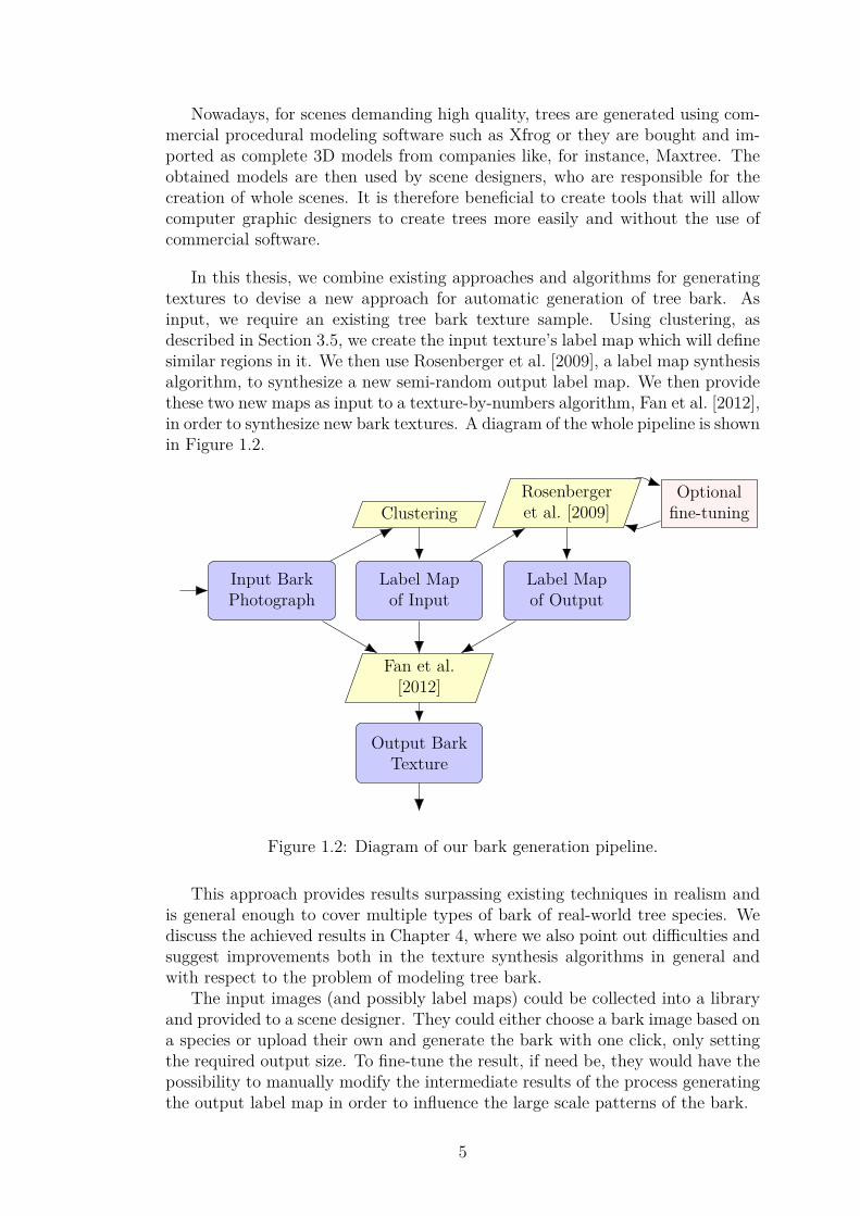
In this thesis, we combine existing approaches and algorithms for generatingtextures to devise a new approach for automatic generation of tree bark. Asinput, we require an existing tree bark texture sample. Using clustering, asdescribed in Section 3.5, we create the input texture’s label map which will definesimilar regions in it. We then use Rosenberger et al. [2009], a label map synthesisalgorithm, to synthesize a new semi-random output label map. We then providethese two new maps as input to a texture-by-numbers algorithm, Fan et al. [2012],in order to synthesize new bark textures. A diagram of the whole pipeline is shownin Figure 1.2.

Label Mapof Input

Input BarkPhotograph

Label Mapof Output

ClusteringRosenbergeret al. [2009]

Fan et al.[2012]

Output BarkTexture

Optionalfine-tuning

Figure 1.2: Diagram of our bark generation pipeline.

This approach provides results surpassing existing techniques in realism andis general enough to cover multiple types of bark of real-world tree species. Wediscuss the achieved results in Chapter 4, where we also point out difficulties andsuggest improvements both in the texture synthesis algorithms in general andwith respect to the problem of modeling tree bark.

The input images (and possibly label maps) could be collected into a libraryand provided to a scene designer. They could either choose a bark image based ona species or upload their own and generate the bark with one click, only settingthe required output size. To fine-tune the result, if need be, they would have thepossibility to manually modify the intermediate results of the process generatingthe output label map in order to influence the large scale patterns of the bark.

5

Our main contribution is the design of a new method for procedural generationof tree bark. As there exist no implementations of the chosen algorithms by Fanet al. [2012] and Rosenberger et al. [2009] used in this method, a significantportion of the work will be the reimplementation of these known algorithms.

6

2. Previous WorkIn this Chapter, we first present a brief overview of existing techniques for proce-dural modeling of trees in Section 2.1. We then talk about tree bark and classifyit in into multiple categories in Section 2.2. In Section 2.3, we discuss previ-ous attempts at procedural modeling of tree bark. Since we will use methodsof texture synthesis to model and generate tree bark in this thesis, we present aclassification of textures in Section 2.4.1 and then provide an overview of existingtexture synthesis algorithms in Section 2.4.2. Lastly, in Section 2.4.3, we brieflydiscuss the possibility of utilizing neural networks.

2.1 Procedural Modeling of TreesThe creation of botanical tree computer models is a complex task requiring spe-cialized modeling methods, Shek et al. [2010]. One of the first methods in-troduced for tree modeling were Lindenmayer-systems (also called L-systems),Prusinkiewicz and Lindenmayer [1990]. L-systems are a formal grammar withwhich one can model trees and plants by defining special rules and by hand-tuning parameters. Barron et al. [2001] later introduced a method for proceduralmodeling of tree movement in the wind and in the rain.

When a high-quality tree model is needed, a valid possibility is recreatingan actual real-world tree by the means of three-dimensional laser scanning, seeXu et al. [2007]. Livny et al. [2011] devised a method of encoding an inputtree model using an intermediate representation called lobes that represent theindividual subsections of three-dimensional space taken up by leaves and branchesto capture overall tree shape.

TreeSketch, introduced by Longay et al. [2012], is an approach to tree mod-eling with which artists may produce trees of varying shapes in just a few brushstrokes. Often, the structure of a tree does not need to be designed. It onlyneeds to match its surroundings. When growing, trees accommodate for nearbyobstacles such as buildings, walls or other trees. Pirk et al. [2012] created a treemodel that self-adapts and changes shape when presented with a nearby obstacle.

2.2 Types of Tree BarkTree bark is the protective outer layer of a tree completely covering its trunk,branches and roots. The process of bark formation is very complex - even morecomplex than that of wood. Many patterns found on tree bark are created bythe interaction of the two different tissues that play a role in bark formation.In comparison, wood is composed of only one tissue. Bark is also exposed toexternal factors such as weather, injury or disease that all contribute to its visualappearance. The physical and other processes in bark formation differ amongbark types.

Dendrologists often classify tree bark into various categories. These tree barktypes are largely arbitrary and differ from author to author. Nevertheless, havingsuch a classification helps with the recognition of tree species. It is however

7

important to note that bark structure changes significantly during the lifespanof a tree. It is common, that a tree may be assigned to multiple bark categoriesdepending on its age. Bark category may even differ among different branches ofthe same tree.

Vaucher [2003] classifies bark into 18 types. There exist more classificationsand Vaucher himself warns, that his classification is entirely arbitrary. In Fig-ure 2.1, you can see an incomplete classification heavily inspired by his work.

(a) 1: Bark smooth,bumpy; thin. Carpinusbetulus.

(b) 2: Bark with shallow,vertical fissures; thin. Acercapillipes.

(c) 3: Bark with deep, ver-tical furrows; thick. Cas-tanea sativa.

(d) 4: Bark with interlac-ing ridges; thick and hard.Fraximus excelsior.

(e) 5: Bark divided intorectangular blocks by deepfissures; thick and hard.Diospyros melanoxylon.

(f) 6: Corky bark wirhraised rhytidomes; thickand hard. Phellodendronamurense.

Figure 2.1: Types of bark.

2.3 Procedural Modeling of Tree BarkOnly a handful of papers were published on the topic of modeling tree bark.Bloomenthal [1985] created one of the first works concerned with the modelingof trees. He modeled tree bark using a digitized bump-map of actual maple barkusing plaster and an x-ray. The bump-map was then overlapped at its sides fora seamless mapping.

Trees are commonly being covered by bark textures using simple texture map-ping. Most often, a single bark image is taken, used multiple times and blended.An overview of texture mapping approaches specifically suited for covering anentire tree with a bark texture, including a list of several blending approaches,can be found in Maritaud [2003].

8

Some of the first bark models were those of Federl and Prusinkiewicz [1996]and Federl and Prusinkiewicz [2002]. They used a mass-spring model and createda physics-based simulation of fractures in bi-layered materials such as tree barkor drying mud. Inspired by their work, some of the most promising results oftree bark synthesis are likely due to Lefebvre and Neyret [2002]. Their modelis also based upon the physics of fractures. It is applicable to all fracture-basedbarks, such as the bark of a fir tree. The appearance of the generated bark isadjustable by the user through parameters of their algorithm. These includeamong others bark stiffness, fracture density and fracture shape. The generatedfractures were mapped onto a three-dimensional tree model and mapped withtextures containing fine-grain details of both the fracture interior and the outerbark layer. These textures were to be created by a skilled artist - once for a giventree species. Desbenoit et al. [2005] later built up upon this method and modeledcracks and fractures on a large variety of surfaces, including wood. Methods forcreating realistic-looking bark using GPU shaders can be found in Ricklefs [2005].

Wang et al. [2003] produced models of tree bark of very high quality. However,they were not concerned with generating tree bark. They proposed a sequenceof methods and implemented a software tool for the end user who could thenconstruct a height-map of a provided bark image. They then used this height-map to filter out shadows from the original bark photograph by an estimatedposition of a single light source. Finally, they proposed an appropriate renderingmethod.

Another notable model of tree bark is that of Dale et al. [2014]. Their goal wasnot to procedurally generate bark for use in computer animated scenes. Instead,it was to describe the biological process of bark creation. They created a bio-mechanical model of a single tree, namely xanthorrhoea, commonly known as thegrasstree. Parameters adjust the overall appearance. Their simulation capturedthe growth of the tree along with the aging of its bark.

To further improve the quality of tree bark, one may add additional featuressuch as mold on top of the bark. See Joshua [2005] for mold modeling. J. et al.was capable of deforming tree bark around objects such as street signs or fences.

2.4 Generating TexturesTexture synthesis is the process of creating (usually large) digital images from asmall sample image. It aims to create images of a given size as similar to theoriginal image as it can. Visual artifacts, such as repeating copy-pasted structuresor seams, should be kept at a minimum.

2.4.1 Types of TexturesAccording to Lin et al. [2004], textures may be classified into a spectrum ofregular, near-regular, irregular, near-stochastic and stochastic textures as seenin Figure 2.2 1. Stochastic textures are completely random textures and lookalmost like noise. These are the easiest to synthesize, since they exhibit no large

1Reused from https://commons.wikimedia.org/wiki/File:Texture_spectrum.jpg on18th May 2018

9

scale patterns visible to a human observer. On the opposite extreme of thespectrum are regular textures, which can be created by periodically repeatinga small shape or pattern by tiling it in equal intervals. Near-regular texturesinclude for example weaved baskets, cloth or brick walls. Near-stochastic texturesare images generated by nature in a random fashion such as grass, clouds or watersurfaces. Irregular textures are the ones in between these two extremes. Theyinclude most day-to-day photographs of objects.

Figure 2.2: Texture spectrum by James Hays of Lin et al. [2004].

Often, a simpler terminology is used. Non-homogeneous textures refer toirregular textures of the texture spectrum, while homogeneous textures are eitherregular or stochastic textures. Homogeneity may be described from a statisticalpoint of view. Homogeneous textures have equivalent statistical properties in allregions. At least when the region size is chosen appropriately.

2.4.2 Overview of Texture Synthesis AlgorithmsTexture synthesis algorithms can be classified into pixel-based, patch-based andoptimization-based methods. Recently, also into methods based on neural net-works.

First, let us discuss some of the simplest, most specific, texture synthesis meth-ods. They usually work on a very narrow set of textures. These include stochastictexture synthesis, single purpose structured texture synthesis and others. Thereare also other techniques based upon tiling, blending and seam reduction.

Pixel-based methods are based on copying pixels from the input texture tothe output texture one at a time. Some of the most notable pixel-based methodsinclude Efros and Leung [1999], Wei and Levoy [2000] and Hertzmann et al.[2001]. These methods may not only be used for synthesizing two-dimensionaltextures, but also for synthesizing textures directly on three-dimensional objects.

Patch-based methods copy whole coherent patches from the input texture tothe output texture. These methods include Liang et al. [2001], Efros and Freeman[2001] and Kwatra et al. [2003]. These methods are susceptible to discontinuitiesalong the edges of individual patches. Wu and Yu [2004] introduced FeatureMatching to prevent breaking of features important to the human visual system,such as edges. They first create feature maps that locate these features. Then,they modify previous algorithms to increase continuity along the feature map.

10

Optimization-based methods first define an energy function that correspondsto the similarity between the input texture and the output texture. An initialoutput texture is generated. This initial output texture is iteratively modified,which causes the optimization of the energy function. One of the most notableoptimization methods is that of Kwatra et al. [2005]. The two algorithms weimplement in Section 3.3 and in Section 3.6 are based on this algorithm.

A more detailed overview of texture synthesis methods can be found in Weiet al. [2009]. They also state that patch-based and optimization-based meth-ods are more successful at synthesizing two-dimensional images than pixel-basedmethods. Meanwhile, pixel-based methods perform well when synthesizing tex-tures directly on three-dimensional objects.

2.4.3 Neural Networks for Texture SynthesisRecently, neural network-based approaches are being introduced. These includeGatys et al. [2015], Gatys et al. [2016], Ustyuzhaninov et al. [2016] and Wilmotet al. [2017]. These approaches mostly use convolutional neural networks tosynthesize textures. This may be due to the fact, that convolutional neuralnetworks closely resemble Gaussian image pyramids often used in classic texturesynthesis algorithms.

When beginning work on this thesis, we decided against the use of neuralnetworks due to a limited amount of literature and few available out-of-the boximplementations. We were aiming to create a method capable of modeling treebark based on a single small input bark photograph. We were concerned by thefact, that neural networks in general require large datasets and computationalresources for training. We later learned that this is not always the case. Formore information, see Ulyanov et al. [2017].

During the work on this thesis, the following implementations of image anal-ogy and texture syntheses algorithms were being created independently of ourwork: Neural Doodle (based on Li and Wand [2016]) Deep Textures, and ImageAnalogies. These implementations might be a good alternative to the algorithmwe implemented and described in Section 3.3.

11

12

3. Tree Bark GenerationIn this Chapter, we describe our proposed tree bark texture synthesis pipelinealong with all implemented algorithms. We start with Section 3.1, where wedescribe the Image Analogy framework. We then give an overview of our wholepipeline in Section 3.2, where we describe how the individual pipeline compo-nents fit together and how they fit into the Image Analogy framework. A majorcomponent of the pipeline, texture-by-numbers by Fan et al. [2012], is describedin Section 3.3. In Section 3.4, we describe a texture-by-numbers initializationmethod for increased quality of the resulting bark texture. Aside from an in-put tree bark photograph, texture-by-numbers requires two additional inputs -namely the input label map and the output label map. In Section 3.5, we presenta clustering-based image segmentation method for creating an input label mapfrom an input tree bark photograph. In Section 3.6, we present the algorithm ofRosenberger et al. [2009] for generating an output label map from an input labelmap.

3.1 Image AnalogiesImage Analogies is a framework for processing images by example by Hertzmannet al. [2001]. Using this method, when given an input image A, a filtered versionof the input image A′ and an unfiltered version B of the wanted output image,we are able to create a filtered output image B′. B′ should visually relate to (beanalogous to) B in the same manner as A′ relates to A.

Applications of image analogies include creating arbitrary image filters, tex-ture synthesis, super-resolution, texture transfer, artistic filters and texture-by-numbers.

The simplest application is texture synthesis. In this case, the images A andB are not used or left blank. Since there is nothing else to guide the analogyprocess except for the input image A′, the output image B′ is created as if thewhole framework were just a texture synthesis algorithm.

When performing texture-by-numbers with the image analogy framework, theimages A and B are used as discrete label maps, where pixels of A′ and B′ aregrouped into regions marked as having the same color at their respective positionsin A and B. Changing the color of a region in both A and B to a different unusedcolor should ideally have no impact. This property is not true for the remainingapplications of image analogy. Due to this reason, one can design algorithmstaking advantage of this specific property and implement a texture-by-numbersalgorithm only instead of the whole image analogy framework.

3.2 Method OverviewNow that we understand the image analogies framework (Section 3.1), we canproceed with the explanation of the pipeline we use to generate tree bark. Theinput of our algorithm is a small photograph capturing tree bark details. Theinput must contain examples of all patterns we want to generate on the resulting

13

tree bark. Our aim is to be able to generate many different output images oftree bark at random, given a desired output size. Of course, we want the outputimages to be as visually close to the input as possible.

First, we generate the input label map A from the input image A′, as describedin Section 3.5. Then, using the algorithm described in Section 3.6, we generatethe output label map B from the generated input label map A. Since now we havethe images A′, A and B, we can use texture-by-number (Section 3.3) to generatethe output image B′, which is the output of our whole pipeline. Notice thecorrespondence to the diagram in Figure 1.2. In addition, Section 3.4 describesa sophisticated method of providing an initial input to the texture-by-numbersalgorithm, greatly increasing quality of the final output.

A nice feature of our approach is that we are using multiple algorithms ina sequence and that these algorithms themselves have intermediate results, cor-responding to finer and finer details of synthesis. This means, that if the userwants more control over the resulting image, they can stop the computation atany time, manually modify the image corresponding to an intermediate result,and let the pipeline run its course and complete all the fine-grained detail theuser does not want to deal with anymore.

3.3 Texture-by-NumbersTexture-by-numbers is an integral part of our pipeline. This method is capableof synthesizing non-homogeneous images with global-varying patterns. We usethis algorithm to generate the final resulting tree bark texture based on the user-provided input and additional images generated specifically for it using all otheralgorithms of our pipeline. Those are described in the following Sections of thisChapter. Existing texture-by-numbers algorithms bordering with the state-of-the-art (not considering neural-network based approaches) include Busto et al.[2010], Sivaks and Lischinski [2011] and Fan et al. [2012].

For our implementation, we have chosen Fan et al. [2012]. Their algorithmbuilds upon the research of Sivaks and Lischinski [2011]. Choosing to implementan improved version of a given algorithm made more sense to us.

The chosen algorithm offers a more complete pipeline, improving the synthesisprocess in several parts of the framework. The core idea behind the algorithmis based upon texture optimization as introduced by Kwatra et al. [2005]. Thechosen framework improves previous results by utilizing a sophisticated initial-ization step based on Bonneel et al. [2010] instead of random initialization, seeSection 3.4 for details. To further improve synthesis quality, a distance metric canbe specified based on texture type, see Section 3.3.4. For structural textures, Fanet al. [2012] define a distance metric utilizing a feature distance map inspired bythe work of Wu and Yu [2004], as previously used in Lefebvre and Hoppe [2006].Also, the chosen algorithm is parallelizable on a GPU using CUDA.

Busto et al. [2010] is mainly concerned with one of the most important stepsof the algorithm - the nearest neighbor search strategy - which we discus fur-ther in Section 3.3.6. They aim to improve upon parallel k-coherence search

14

by introducing their own search strategy called parallel randomized correspon-dence. However, in comparison to Fan et al. [2012], the approach of Busto et al.[2010] was not yet implemented and tested on a GPU. Our chosen frameworkalso claims, that their improvements provide a similar quality increase to thatof randomized correspondence. In addition, it should be possible to improve ourimplemented texture-by-numbers framework by simply substituting k-coherencesearch by parallel randomized correspondence. This is left as future work.

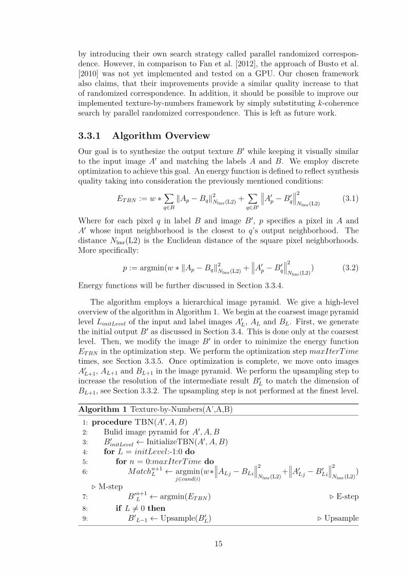
3.3.1 Algorithm OverviewOur goal is to synthesize the output texture B′ while keeping it visually similarto the input image A′ and matching the labels A and B. We employ discreteoptimization to achieve this goal. An energy function is defined to reflect synthesisquality taking into consideration the previously mentioned conditions:

ET BN := w ∗∑q∈B

∥Ap −Bq∥2Nlmr(L2) +

∑q∈B′

A′p −B′

q

2

Nlmr(L2)(3.1)

Where for each pixel q in label B and image B′, p specifies a pixel in A andA′ whose input neighborhood is the closest to q’s output neighborhood. Thedistance Nlmr(L2) is the Euclidean distance of the square pixel neighborhoods.More specifically:

p := argmin(w ∗ ∥Ap −Bq∥2Nlmr(L2) +

A′p −B′

q

2

Nlmr(L2)) (3.2)

Energy functions will be further discussed in Section 3.3.4.

The algorithm employs a hierarchical image pyramid. We give a high-leveloverview of the algorithm in Algorithm 1. We begin at the coarsest image pyramidlevel LinitLevel of the input and label images A′

L, AL and BL. First, we generatethe initial output B′ as discussed in Section 3.4. This is done only at the coarsestlevel. Then, we modify the image B′ in order to minimize the energy functionET BN in the optimization step. We perform the optimization step maxIterT imetimes, see Section 3.3.5. Once optimization is complete, we move onto imagesA′

L+1, AL+1 and BL+1 in the image pyramid. We perform the upsampling step toincrease the resolution of the intermediate result B′

L to match the dimension ofBL+1, see Section 3.3.2. The upsampling step is not performed at the finest level.

Algorithm 1 Texture-by-Numbers(A’,A,B)1: procedure TBN(A′, A, B)2: Bulid image pyramid for A′, A, B3: B′

initLevel ← InitializeTBN(A′, A, B)4: for L = initLevel:-1:0 do5: for n = 0:maxIterT ime do6: Matchn+1

L ← argminj∈cand(i)

(w∗ALj −BLi

2

Nlmr(L2)+

A′Lj −B′

Li

2

Nlmr(L2))

▷ M-step7: B′n+1

L ← argmin(ET BN) ▷ E-step8: if L = 0 then9: B′

L−1 ← Upsample(B′L) ▷ Upsample

15

Pixel Neighborhood

When referring to a pixel neighborhood in this thesis, we always mean its squareneighborhood. A neighborhood N(p) centered on a pixel p in an image at a givenindex is further defined by the neighborhood size. This is an algorithm parameterthat needs to be fine-tuned by the user. A neighborhood’s size denotes the lengthof a side of the square defining the neighborhood. Only odd sizes are acceptable.

Nlmr(p) denotes of full square neighborhood. The individual letters stand for left,middle and right. The number of pixels in this type of neighborhood of size issize2.

Nlr(p) denotes of a square neighborhood with the middle pixel p left out. Theindividual letters stand for left and right. The number of pixels in this type ofneighborhood of size is size2 − 1.

Image of References

The optimization works by copying pixels from the input image A′ to the outputimage B′. The algorithm requires us not only to keep a color value of all pixels ofthe synthesized image B′, but we must also keep a reference to the source imagepixel from which the pixel is copied over. The algorithm will use the knowledge ofthe neighborhood of that pixel to its advantage in k-coherence search and duringforward-shifting. Since we already have the information about pixel positions, wewill also use it later during upsampling when increasing the synthesized imageresolution. B′ will thus be an image of references.

Using this fact and the fact that the energy function essentially only usesthe squared Euclidean distance, we can change the number of channels of theinput image A′ arbitrarily. We can for example add a height-map correspondingto A′ as a fourth channel and the algorithm we generate an output height-mapcorresponding to B′ without any extra effort. As a plus, this may actually increasesynthesis quality, as if in were a feature distance map. See Section 3.3.4 for moredetails.

Forward-Shifted Pixel Neighborhood

For each referenced pixel in the input neighborhood, we compute an appropriatelyforward shifted reference based on relative pixel positions, as visually explainedin Figure 3.1. The illustration is using wrap.

When using wrap, forward-shift pixels across neighborhood boundaries.When not using wrap, output NaN instead of crossing neighborhood boundaries.

16

A B C DE F G HI J K LM N O P

(a) Referenced image

A F HC L PG L I

(b) Neighborhood ofreferences

F J KD L OD H H

(c) Forward-shiftedneighborhood of

references

Figure 3.1: Illustration of forward-shifting.

3.3.2 Hierarchical Image PyramidImages are kept in an image pyramid. This way, we can first optimize images at alow resolution to focus on large scale patterns. When maxIterT ime optimizationsteps were performed at a given pyramid layer, we move on to the next level.We must also increase the resolution of the synthesized image. This is doneby upsampling. The pyramid itself is created by first calculating image sizesat individual pyramid levels and then downsampling the original images to thesesizes. We must take care that the indices used in the downsampled and upsampledimages match at each pyramid level. These two operations must be inverse toeach other.

Pyramid Level Size Computation

Given an input image size and a number of levels, we will calculate the image sizesat individual pyramid levels. We always want to keep both the number of pyramidlevels and the lowest resolution size at a minimum. Somewhat arbitrarily, we willadopt the strategy of always doubling both the image width and hight when goingup the pyramid when possible. This may be impossible for the level at the finestresolution, where we may have to increase the sizes by less then a factor of two.

Downsampling

We will usually downsample by a factor of two. This means to simply removingevery other row and column and recomputing references. However, during ourfirst downsampling, we may have to downsample by less than a factor of two.Then we downsample the images by uniformly removing rows and columns fromthe input image. We never remove two rows or columns that are next to eachother. This will allow us to perform upsampling. We however need to make sure

17

that we add back the exact same rows and columns during upsampling as weremoved during downsampling.

Upsampling

The upsampling step is performed in order to increase the resolution of an imageof references by a factor of 2 or less. Pixel references must first be recomputed.We now add rows and columns matching the positions from which downsamplingremoves rows and columns. Each newly created pixel inherits an appropriatelyshifted coordinate of its left, top or top-left neighbor. An illustration of upsam-pling pixel q in B′

L−1 when generating B′L is shown in Figure 3.2.

q r

s t

(a) Referenced image A′L.

q

(b) Image of referencesB′

L−1 before upsampling.

q r

s t

(c) Image of referencesB′

L after upsampling.

Figure 3.2: Illustration of upsampling.

3.3.3 Approximate Nearest Neighbor SearchOne of the most computationally expensive steps of the algorithms we implementin this thesis is nearest neighbor search. Given a dataset of points in an arbitrarydimension and a testset of points in the same dimension, the goal of k-nearestneighbors is to find for each point in the test set, k points in the dataset, whichare closest under a given metric. In this thesis, we will always use the squaredEuclidean metric with k-nearest neighbors. There are no known algorithms forsolving this problem faster than by linear search. Given our use case, this istime complexity unacceptable. However, an approximate nearest neighbor searchgives results comparable to the exact search. They are at least for more thangood enough for our purposes.

The only external algorithm library used when implementing the algorithmsof Fan et al. [2012] and of Rosenberger et al. [2009] is the FLANN library, Mujaand Lowe [2014], for computing approximate nearest neighbors. More possibilitiesexist. However, we did not pursue them. For example, Fan et al. [2012] suggeststhe use of Tang et al. [2012] and claims faster computation time on images ofsizes ≤ 256 ∗ 256 pixels. That would cover most of the images we generated.

3.3.4 Distance Metric of Texture SimilarityFor images exhibiting structural patterns, such as clearly defined edges and ridges,the L2 distance of image neighborhood is not sufficient. The human visual system

18

places an extra value on edges and ridges. To take this into account, we canmodify the energy function as follows:

ET BN := w ∗∑q∈B

∥Ap −Bq∥2Nlmr(L2) + z ∗

∑q∈B′∥FDMp − FDMq∥2

Nlmr(L2)

+∑

q∈B′

A′p −B′

q

2

Nlmr(L2)

(3.3)

Alternatively, we can keep the energy function the same. We just consider FDMas an additional image channel of A′.

Coefficients w and z determine the importance of the label and feature dis-tance channels respectively. These parameters need to be adjusted properly forgood output image quality. The value of these coefficients chosen by Fan et al.[2012] were w = 1 and z = 3. In our bark generation pipeline, we found goodperforming values to be w = 3 and z = 8. It however depends on a given set ofinputs.

More information about the calculation of feature distance maps can be foundin Lefebvre and Hoppe [2006].

3.3.5 Discrete Solver Based on k-coherenceThis discrete optimization solver we employ was introduced by Han et al. [2006]and is an adaptation of the original EM-like texture optimization framework byKwatra et al. [2005]. The original adaptation utilized a hierarchical tree searchfor the M-step and least-squares for the E-step. The hierarchical tree search wasthe computational bottleneck with a time complexity of O(log(N)) where N wasthe number of input pixels. k-coherence 3.3.6 has constant time complexity persearch while keeping satisfactory quality, as stated by Lefebvre and Hoppe [2005].

The least squares method originally used in the E-step is incompatible withk-coherence and must be changed as a consequence. In particular, k-coherencestores references to pixels in the exemplar in the synthesized image. This is donebecause k-coherence needs to know the source pixel location of every synthesizedpixel. The least squares method however does direct computation on the RGBvalues in the synthesized image and thus does not allow for direct pixel copyingfrom the exemplar. To overcome this problem, a different E-step was adopted.

One iteration of the discrete solver:

(Inputs):• A′: Input texture image with the optional feature distance map FDM

included as additional channels.• A: Input label map.• B: Output label map.• B′: Output reference image generated in the previous iteration. For gener-

ating the initial B′ before the first discrete solver iteration, see 3.4.

(0) Definitions:

19

Let X and Y be two images of the same shape. Then concat(X, Y ) is animage with all image channels of X and Y concatenated.Let X be an image (or neighborhood) of references. Then Xref is an image(or neighborhood) with references resolved.Let X be an image. Then N(X) is a list of all neighborhoods in X. Thelength of N(X) is the same as the number of pixels in X.Let X be an image of references. N forward shift(X) is the set of all forwardshifted neighborhoods of references in X. The length of N forward shift(X) isthe same as the number of references in X.

(1) Construct a candidate set:A candidate set for each reference in B′ is built using k-coherence search3.3.6.Let x ∈ B′ be a reference. Then cand(x) is the candidate set of x.

(2) M-step: Find best-matching candidate.Let E := concat(A, A′).Let S := concat(B, B′

ref).We want to create an image of references MatchL of the same shape as S.Let X† be a subset of indices of S. The references in MatchL will be definedonly at indices in X†.X† is created by uniformly leaving out pixels of MatchL.For every neighborhood in the subset of the synthesized image, find theclosest neighborhood to it in the exemplar among the coherence candidatesand save its reference into MatchL:

∀i ∈ X† : MatchLi:= argmin

j∈cand(i)(∥Nlr(S)i −Nlr(E)j∥2

L2) (3.4)

(3) E-step: Find candidate minimizing the energy function.Let M := N forward shift

lmr (MatchL)ref be an image of neighborhoods.Create the image Avg by converting each neighborhood into a single pixelby taking the channel-wise average over all neighbors. Undefined neighborsdo not take part in the average computation.Let T := concat(B, M).Let I be the set of indices in T .For every pixel in the synthesized image, take the channel-wise average ofthe corresponding forward shifted neighborhood in MatchL, find the closestpixel to it in the exemplar among the coherence candidates and save itsreference into BL:

∀i ∈ I : BLi:= argmin

j∈cand(i)(∥Ti − Ej∥2

L2) (3.5)

20

(Output):• B′

L: The new reference image. It should be converted to B′Lref

after the lastiteration.

3.3.6 k-coherence SearchIn many texture-by-numbers algorithms, we repeatedly replace each synthesizedpixel by the exemplar pixel with most the similar neighborhood. As this is afrequent and expensive step, multiple search strategies for the most similar pixelexist. They aim at a balance between a fast runtime and a high-quality output.

These nearest neighbor search strategies include:• Coherence search by Ashikhmin [2001].• k-coherence search by Tong et al. [2002].• Patch Match by Barnes et al. [2009].• Coherent random walk method by Busto et al. [2010].

In this thesis, the texture-by-numbers framework we chose to implement wasFan et al. [2012]. k-coherence search was the method chosen in this framework,which is why we implemented it. Newer methods, such as coherent random walk,show promising results by improving synthesis quality while maintaining fastsynthesis times. As future work, it would be beneficial to implement these newermethods to try and improve our bark synthesis pipeline.

Computation of k-coherence search:Let B′ be an image of references to pixels in the image A′.For each pixel p0 ∈ B′, we want to compute the candidate set C(p0).

First, we need a precomputed list of (k − 1)-nearest neighbors for each pixelin the image. We use the FLANN library. (Both the dataset and the testsetcontain all image pixels).

Next, we compute coherence candidates C1(p0) of pixel p0 ∈ B′:

• We denote Nlmr(p0) the set of pixels in the neighborhood of p0.

• Every pixel p ∈ Nlmr(p0) corresponds to a pixel p′ ∈ A′.

• We can then compute p′′ by forward-shifting p′.

• Forward-shifting means that the difference in coordinates between p′ andp′′ ∈ A′ is the same as the difference in coordinates between p and p0 ∈ B′.

• The set of all possible pixels p′′ is the coherence candidate set C1(p0).

Finally, the candidate set C(p0) of k-coherence search is created as a union ofthe coherence candidate set C1(p0) and the precomputed lists of (k − 1)-nearestneighbors for each pixel in C1(p0).

21

3.4 Texture-by-Numbers Initialization

3.4.1 Random InitializationOriginally, the texture optimization framework initialized the algorithm by copy-ing random pixels from the input to the output. A slightly improved techniquecopies random neighborhoods from the input to the output. A simple texture-by-numbers adaptation would be to only assign pixels or neighborhoods withincorresponding label map regions.

While a simple initialization is sufficient for homogeneous textures, synthesisof non-homogeneous textures may be significantly improved by better initializa-tion. In fact, we have found that a high quality result during bark synthesisfor certain types of bark may be achieved by simply utilizing texture synthe-sis (not even texture-by-numbers) with this more sophisticated initialization, seeSection 4.1. An illustration of the effect a proper initialization can have on thequality of the result is shown in Figure 4.4. Fan et al. [2012] also notes an in-creased runtime speed in his implementation due to faster convergence of thelater optimization compared to a random initialization.

3.4.2 Texture Synthesis Based InitializationAs a sophisticated initialization for the optimization of texture-by-numbers, weuse the first pass of the fast guided texture synthesis method of Bonneel et al.[2010]. In the cited paper, a texture-by-numbers algorithm is also being created.However, their goal is to use this algorithm to quickly and easily synthesize three-dimensional scenes. Fan et al. [2012] decided to only use only the first pass of thisother texture-by-numbers algorithm as initialization for our texture-by-numbersalgorithm, as it is fast and improves results. It would also be interesting to know,if further increase in synthesis quality would be gained by also implementing thesecond pass, or if the optimization we perform would renders it unnecessary. Thisis left as future work.

To initialize the optimization of texture-by-numbers, we create an approxi-mate texture-by-numbers result by using chamfer distance as a metric in a regiongrowth method. The initialization process proceeds as follows:

First, discrete label maps must be generated: IDA from A and IDB from B.Pixels of a similar color in the label map must be mapped into one discrete value.In Figure 3.3, this is visualized by gray-scale values. An edge detection algorithmis then used to locate all borders between different discrete label regions. Finallythe 3-4 DT method of Borgefors [1988] is used to produce distance maps DA andDB. Distance maps mark the approximate distance of each pixel from the closestpixel of a different discrete label region.

Now that we have computed the necessary chamfer distance, we can definethe following metric:

d(pA, pB) := w ∗ ∥IDApA− IDBpB

∥Nlmr(chamfer) + ∥DApA−DBpB

∥Nlmr(L2) (3.6)

22

Where w = 90. In the last step, we first create a blank image initB. We randomlyselect seeds to grow in initB and grow it using a floodfill algorithm. The regiongrowth stop condition is d(pB, p′

B) < t. t is defined as (d(pA, pB) + 5) ∗ 1.25.pB ∈ IDB is the seed of the floodfill algorithm. pA ∈ IDA is the pixel nearest topB under the Equation (3.6). p′

B is a pixel neighboring the region being seededby pB and it is a candidate to join the region if it fulfills the condition specifiedfor the floodfill algorithm.

This method is an example of a patch-based texture synthesis algorithm wherethe input and output label maps provide extra inputs in addition to the originalimage. This initialization process could also be parallelized to facilitate GPUsynthesis.

(a) A (b) IDA (c) A edges (d) DA

(e) B (f) IDB (g) B edges (h) DB

(i) A’ (j) initB (k) colorInitB

Figure 3.3: Illustration of generation of initial output.

3.5 Input Label Map GenerationGeneration of an input label map for the texture-by-numbers framework is tra-ditionally left to the user. In general, it is not easy to determine the individualregions present in an image nor the number of regions present. It not only dependson the image itself, but also on our overall goal. In fact, image segmentation is asignificant area of research in computer science.

We are however only interested in the specific case of bark textures. Wewould like to capture large-scale patterns in tree bark by mapping pixels into kregions (usually k <= 5). This would correspond to key bark attributes suchas fractures, lenticels, furrows, fissures, flaking patches, etc. For this purpose,a clustering-based method into regions of similar colors will be sufficient. Theamount of colors corresponds to the parameter k. This parameter will depend

23

mostly on the type of bark and the artifacts present in the bark. Hierarchicalclustering methods could relieve the user from having to specify this parameter.However, there are only few possible choices. Also the performance of the otheralgorithms in our bark generation pipeline depends heavily on the choice of k, aswill be discussed in Chapter 4. For these reasons, k is left to be specified by theuser.

This whole process is illustrated in Figure 3.4.

3.5.1 CIELAB Color SpaceDuring the generation of the input label map, the denoising and quantizationsteps will be performed in the CIELAB (sometimes called Lab) color space, asopposed to the standard RGB color space. CIELAB was designed as a colorspace approximating human vision. The three components are L, a and b. Lclosely matches the human concept of lightness and a and b are green-red andblue-yellow color components. This conversion into CIELAB and back greatlyincreases the quality of our algorithm.

3.5.2 DenoisingAs preprocessing of the quantization step, we will denoise the image in order toremove small-scale patterns in the image. Figure 3.4b shows a denoised image.The task of denoising is the opposite of adding random noise to the image. Oneof the motivations behind denoising algorithms is the removal of noise generatedby the process of taking a photograph with a digital camera. When using thismethod, more coherent regions are created in the quantization step. We havechosen the non-local means denoising algorithm by Buades et al. [2011], which iscurrently implemented in OpenCV as cv::fastNlMeansDenoisingColored.

It is important that this step looks at the neighborhood of a given pixelwhen creating its denoised counterpart. This is useful, since humans do not onlyconsider the absolute pixel color as important when recognizing regions, but alsodiscontinuities such as edges or ridges. In a similar algorithm for creating inputlabel maps by Rosenberger et al. [2009], the quantization is performed using k-means on pixel neighborhoods instead of pixels. For us, quantization of pixels issufficient thanks to this denoising step.

3.5.3 QuantizationThe MiniBatchKMeans clustering algorithm is used to cluster the denoised clus-ters converted into CIELAB color space into k clusters. This reduces the numberof colors present in an image to k. The individual colors of the result correspondto the k individual regions of the label map. Figure 3.4c shows a quantized image.

3.5.4 ErosionSometimes, the quantization creates very small regions of one or just a few pixelsinside a huge monolithic region. Such tiny regions are undesirable. An erosionstep further improves the result. A simple heuristic is employed: Each pixel

24

becomes its most common neighbor. Figure 3.4d shows an image after erosionwas applied.

3.5.5 Grayscaling and Edge DetectionSince we only care about designating regions on an images, the actual k-meanscenter colors are unimportant. It is sufficient to keep a grayscale value. We alsofound that adding a separate region for all edges among the regions found sofar often improves quality of the texture-by-numbers framework. However, thispostprocessing adds complexity for the algorithm creating the output label map.Therefore, this step should be performed on both input and output label mapsafter they are both generated. Figure 3.4e shows the final output.

(a) A’ (b) Denoising (c) Quantization

(d) Erosion (e) Grayscaling and EdgeDetection

Figure 3.4: Illustration of Label generation.

25

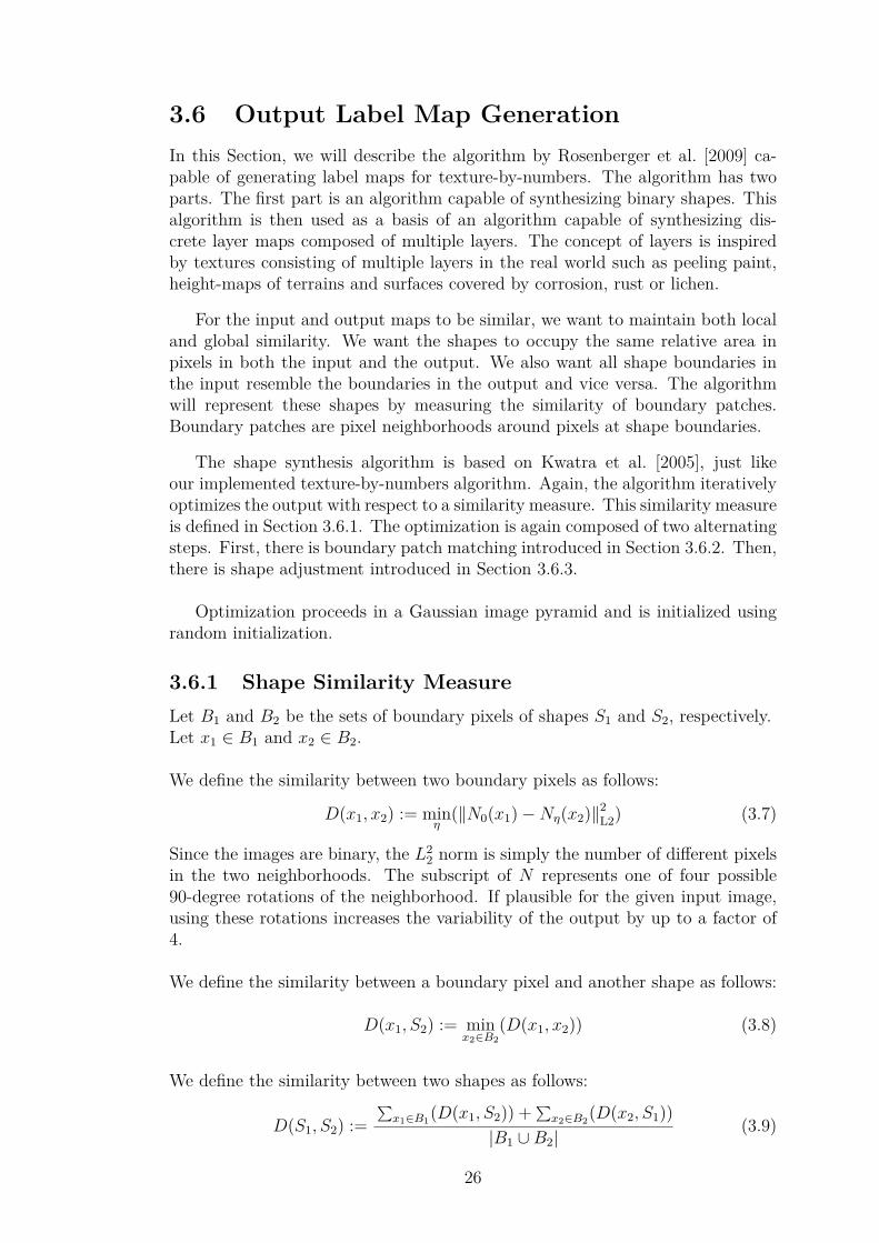
3.6 Output Label Map GenerationIn this Section, we will describe the algorithm by Rosenberger et al. [2009] ca-pable of generating label maps for texture-by-numbers. The algorithm has twoparts. The first part is an algorithm capable of synthesizing binary shapes. Thisalgorithm is then used as a basis of an algorithm capable of synthesizing dis-crete layer maps composed of multiple layers. The concept of layers is inspiredby textures consisting of multiple layers in the real world such as peeling paint,height-maps of terrains and surfaces covered by corrosion, rust or lichen.

For the input and output maps to be similar, we want to maintain both localand global similarity. We want the shapes to occupy the same relative area inpixels in both the input and the output. We also want all shape boundaries inthe input resemble the boundaries in the output and vice versa. The algorithmwill represent these shapes by measuring the similarity of boundary patches.Boundary patches are pixel neighborhoods around pixels at shape boundaries.

The shape synthesis algorithm is based on Kwatra et al. [2005], just likeour implemented texture-by-numbers algorithm. Again, the algorithm iterativelyoptimizes the output with respect to a similarity measure. This similarity measureis defined in Section 3.6.1. The optimization is again composed of two alternatingsteps. First, there is boundary patch matching introduced in Section 3.6.2. Then,there is shape adjustment introduced in Section 3.6.3.

Optimization proceeds in a Gaussian image pyramid and is initialized usingrandom initialization.

3.6.1 Shape Similarity MeasureLet B1 and B2 be the sets of boundary pixels of shapes S1 and S2, respectively.Let x1 ∈ B1 and x2 ∈ B2.

We define the similarity between two boundary pixels as follows:

D(x1, x2) := minη

(∥N0(x1)−Nη(x2)∥2L2) (3.7)

Since the images are binary, the L22 norm is simply the number of different pixels

in the two neighborhoods. The subscript of N represents one of four possible90-degree rotations of the neighborhood. If plausible for the given input image,using these rotations increases the variability of the output by up to a factor of4.

We define the similarity between a boundary pixel and another shape as follows:

D(x1, S2) := minx2∈B2

(D(x1, x2)) (3.8)

We define the similarity between two shapes as follows:

D(S1, S2) :=∑

x1∈B1(D(x1, S2)) + ∑x2∈B2(D(x2, S1))

|B1 ∪B2|(3.9)

26

3.6.2 Boundary Patch MatchingLet BE and BS be the set of boundary patches of E and S, respectively.Compute the boundary patch matching using the following greedy algorithm:

1. Assign each patch in BE to its nearest neighbor in BS.2. For each boundary patch s ∈ BS, keep only its nearest assignment.3. Remove all assigned patches from consideration and repeat until all patches

have been matched.Assume, that |BS| = Q |BE|+ R.Create Choice as a random choice of R elements from BE.Each exemplar patch is to be assigned to a synthesized patch precisely Q timesif e /∈ Choice and Q + 1 times if e ∈ Choice.

3.6.3 Shape AdjustmentWe will now increase the similarity of the two shapes by minimizing the energyfunction D(S, E). That is, we modify the boundary of the synthesized imageB(S) by increasing its similarity to the exemplar boundary B(E).

We start by creating weights for pixels near boundaries of the synthesizedimage. These weights determine pixel changes during an iteration. This weightcreation will be done by superimposing each exemplar patch over its counterpartin BS.

We will assign a score to each pixel xS in the vicinity of a boundary in thesynthesized image B(S). The score predicts if the pixel xS should belong to theshape or not. A positive value means that it should be a part of the shape S anda negative value means that it shouldn’t be a part of S. The absolute value ofthe score is a measure of certainty of our prediction. We will only change pixelswith a prediction higher than a certain threshold.

Let xS ∈ B(S) be a synthesized boundary pixel and xE ∈ B(E) its corre-sponding match found in Section 3.6.2. The weights wxS

of the neighborhoodN(xS) are calculated as follows:

wxS:= 1

1 + D(xS, xE) ∗ indicator(xE)⊙ falloff (3.10)

Where ⊙ denotes element-wise matrix multiplication. indicator is +1 if the pixelbelongs the to the given shape and −1 if not. falloff is the Gaussian fallofffunction. This function will make the weight decrease away from the center ofthe patch - a pixel should have more effect on its immediate surroundings thanon the most distant pixels in the neighborhood.

We accumulate the weights of all neighborhoods of pixels in the vicinity of aboundary in the synthesized image B(S) into the weight matrix W . We constructthe weight matrix W by adding wxS

to W at the coordinate of xS for every xS.

A threshold determines pixel changes resulting from a given shape adjustmentstep. The threshold is set dynamically to the value in the interval [10−2, 10−7]

27

which will minimize the relative difference in the amount of pixels between theexemplar and the synthesized image. Convergence is reached after a predefinednumber of iterations or when the number of pixel changes falls below a certainthreshold.

3.6.4 Layer Map GenerationThe shape optimization algorithm presented in the previous Subsections of Sec-tion 3.6 can only synthesize a binary image. However, we want to synthesize alabel map which will possibly have more than two colors.

In order to achieve our goal, we will consider label maps to be layer maps.The difference between the two is that a layer map has an additional orderingof its individual regions while a label map does not. A pixel of a given layer isconsidered to be a part of all lower layers as well. Due to this layer representation,we can decide for every pixel in an image if it belongs to a given layer or not. Wecan thus create a binary image for each layer. The ordering of layers is left tobe specified by user. If the texture is visibly composed of layers, the user shouldspecify this obvious ordering.

The shape optimization algorithm without modification will be used to gen-erate the coarsest layer. We will initialize the algorithm by a randomly generatedbinary image with the number of foreground pixels matching the correspondingexemplar layer. The shapes of all following layers must be nested inside the pre-viously generated shapes. Also, we will aim at preserving correlation betweeneach pair of successive shapes.

The synthesis of each subsequent layer begins by the creation of a mask. Thismask defines the area of the image where the current layer is allowed to synthesizeand grow. Each mask is initially set to the shape of the previous layer and thenis shrunk according to a weight matrix created based on the last boundary patchmatching. We are again superimposing pixels, but this time we are predictingpixels belonging to the subsequent layer. Both the shape of the mask and the layerinitialization are determined by the weight matrix using thresholds. At higherresolutions, a similar step is repeated. However, we only modify the upsampledmask and layer shape based on the thresholds used earlier. We do not recreatethem.

28

29

4. Results and DiscussionIn this Chapter, we present experiments we ran with our pipeline under variousconfigurations. We judge the results and discuss the advantages and shortcomingsof the utilized methods. In Section 4.1, we discuss the quality of the texture-by-numbers algorithm when used only for texture synthesis. At the same time, wediscuss the limits and possibilities of generating bark textures using only texturesynthesis. In Section 4.2, we show the importance of proper initialization ofthe texture-by-numbers algorithm we implemented and state a hypothesis forthe reasons behind the need of that particular initialization. In Section 4.3, weuse our pipeline to generate tree bark using two-color label maps. The use ofmulti-color label maps in the pipeline is discussed in Section 4.4

4.1 Texture SynthesisIn the following Section, we use our implemented texture-by-numbers algorithm(Section 3.3) to perform texture synthesis. No label maps are used.

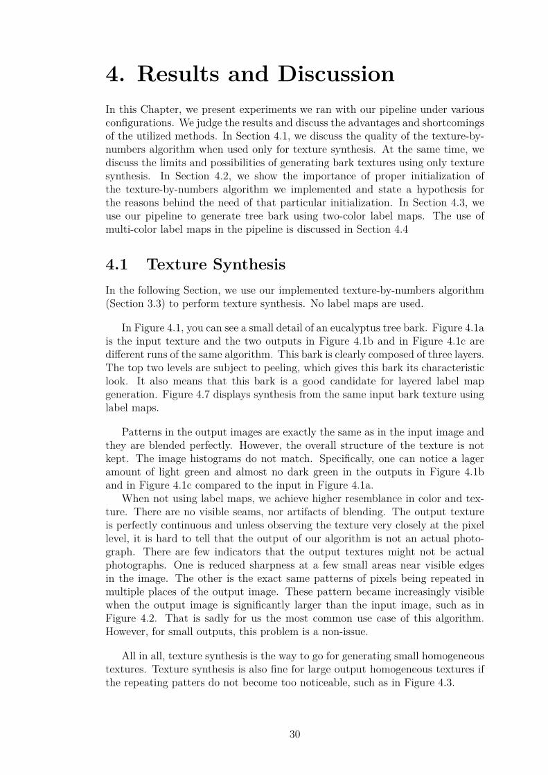
In Figure 4.1, you can see a small detail of an eucalyptus tree bark. Figure 4.1ais the input texture and the two outputs in Figure 4.1b and in Figure 4.1c aredifferent runs of the same algorithm. This bark is clearly composed of three layers.The top two levels are subject to peeling, which gives this bark its characteristiclook. It also means that this bark is a good candidate for layered label mapgeneration. Figure 4.7 displays synthesis from the same input bark texture usinglabel maps.

Patterns in the output images are exactly the same as in the input image andthey are blended perfectly. However, the overall structure of the texture is notkept. The image histograms do not match. Specifically, one can notice a lageramount of light green and almost no dark green in the outputs in Figure 4.1band in Figure 4.1c compared to the input in Figure 4.1a.

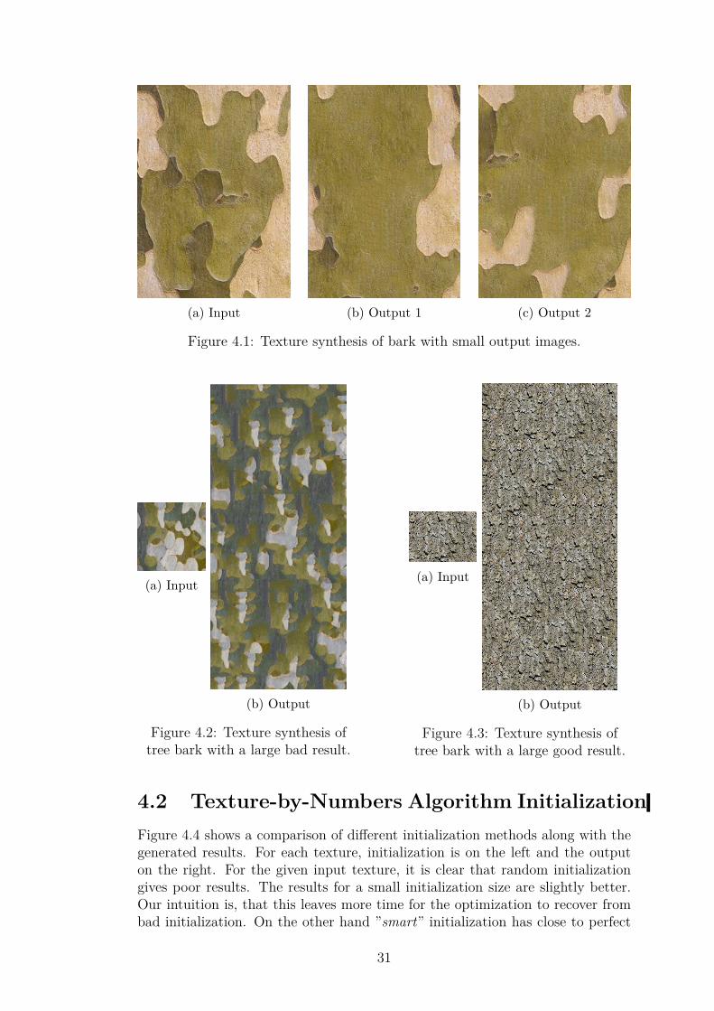
When not using label maps, we achieve higher resemblance in color and tex-ture. There are no visible seams, nor artifacts of blending. The output textureis perfectly continuous and unless observing the texture very closely at the pixellevel, it is hard to tell that the output of our algorithm is not an actual photo-graph. There are few indicators that the output textures might not be actualphotographs. One is reduced sharpness at a few small areas near visible edgesin the image. The other is the exact same patterns of pixels being repeated inmultiple places of the output image. These pattern became increasingly visiblewhen the output image is significantly larger than the input image, such as inFigure 4.2. That is sadly for us the most common use case of this algorithm.However, for small outputs, this problem is a non-issue.

All in all, texture synthesis is the way to go for generating small homogeneoustextures. Texture synthesis is also fine for large output homogeneous textures ifthe repeating patters do not become too noticeable, such as in Figure 4.3.

30

(a) Input (b) Output 1 (c) Output 2

Figure 4.1: Texture synthesis of bark with small output images.

(a) Input

(b) Output

Figure 4.2: Texture synthesis oftree bark with a large bad result.

(a) Input

(b) Output

Figure 4.3: Texture synthesis oftree bark with a large good result.

4.2 Texture-by-Numbers Algorithm InitializationFigure 4.4 shows a comparison of different initialization methods along with thegenerated results. For each texture, initialization is on the left and the outputon the right. For the given input texture, it is clear that random initializationgives poor results. The results for a small initialization size are slightly better.Our intuition is, that this leaves more time for the optimization to recover frombad initialization. On the other hand ”smart” initialization has close to perfect

31

results. It is hard to tell which of the initialization sizes produces a higher qualityresult.

The advantages of ”random” initialization is its ease of implementation andfast runtime. ”Smart” initialization has neither. However, as is seen in Fig-ure 4.4, in certain cases the texture-by-numbers algorithm essentially does notwork properly unless ”smart” initialization is used. We believe that this is dueto the fact that the initialization and optimization steps complement each other.

During the course of optimization, the output texture is blended. It is beingmade more continuous. Breaks and seams in the output are being fixed. However,we do not optimize for the coherence of input patches. We do not support pixelsclose to each other in the input to be in the same relative positions in the output.This is by definition done by patch-based texture synthesis methods. Nor do weoptimize so that all pixels in the input are represented in the output. We do notoptimize for the input and output histograms to match.

The algorithm we use for ”smart” initialization is a simple patch-based texturesynthesis algorithm that copies coherent patches from the input image and triesto cover all of the input image equally. When this coherence is supplied to thetexture synthesis algorithm by the means of initialization, we get a good result.

(a) Input

(b) 32px - random (c) 64px - random (d) 128px - random

(e) 32px - smart (f) 64px - smart (g) 128px - smart

Figure 4.4: Comparison of texture-by-numbers initializations.

32

We therefore propose as future work a possible change to the energy func-tion being optimized by the texture-by-numbers algorithm to account for thiscoherence of pixels and equal representation of the input in the output.

4.3 One-Layer Label MapsLet us first focus on the generated label maps in Figure 4.5. The generatedtwo-color input label map in Figure 4.5b nicely separates the input bark texture(Figure 4.5a) into regions of fracture interiors as the darker color and of the top-most bark layer as the lighter color. We believe that the generated output labelmap in Figure 4.5c exhibits the same patterns as the input label map. We believeit is of very high quality and that it exhibits no visible defects.

If this label map were used successfully, we believe it would improve synthesisquality by fixing problems described in Section 4.1, such as seams or blendingartifacts. It could prevent the repetition of the same input regions over and overagain when generating large output textures and could promote the creation ofnew fracture patterns similar to existing ones by blending them.

The output texture Figure 4.5d generated by our implemented texture bynumbers algorithm is very blurry. Some regions are not blurry, but that is becausethe output label of these regions resembles the input label very closely. An inputtexture region can thus be copied to the output whole.

This is the same kind of blur as seen in Section 4.2. We thus suppose thatthis could be fixed by the improved energy function proposed as future work inSection 4.2 or by improving the texture-by-numbers initialization algorithm fromSection 3.4 on label maps with many small regions. On the other hand, if welook past the blur, all other problems of generating bark textures we describedin previous Sections are fixed.

33

(a) Input Texture (b) Input Label

(c) Output Label (d) Output Texture

Figure 4.5: Texture-by-numbers with 2-color label maps.

4.4 Multi-Layer Label MapsIn the previous Section, we have praised the results of the shape synthesis algo-rithm from Section 3.6 when used on a label map with two colors. In this Section,we will show that the result quality decreases dramatically with the number ofcolors used.

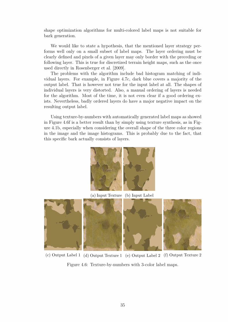
In Figure 4.6, we generate output label maps with three colors and in Fig-ure 4.7, we generate output label maps with five colors. The label map qualityachieved for three colors is still acceptable. We had to however manually choosethe correct layer ordering as described in Section 3.6.4. With five colors, theoutput label is completely different from the input label.

The output quality of the layered shape synthesis algorithm from Section 3.6decreases rapidly with a growing number of layers. This shows that althoughthe shape optimization algorithm for binary images from Section 3.6 is good, asdiscussed in Section 4.3, the layer strategy from Section 3.6.4 to generalize the

34

shape optimization algorithms for multi-colored label maps is not suitable forbark generation.

We would like to state a hypothesis, that the mentioned layer strategy per-forms well only on a small subset of label maps. The layer ordering must beclearly defined and pixels of a given layer may only border with the preceding orfollowing layer. This is true for discretized terrain height maps, such as the onceused directly in Rosenberger et al. [2009].

The problems with the algorithm include bad histogram matching of indi-vidual layers. For example, in Figure 4.7c, dark blue covers a majority of theoutput label. That is however not true for the input label at all. The shapes ofindividual layers is very distorted. Also, a manual ordering of layers is neededfor the algorithm. Most of the time, it is not even clear if a good ordering ex-ists. Nevertheless, badly ordered layers do have a major negative impact on theresulting output label.

Using texture-by-numbers with automatically generated label maps as showedin Figure 4.6f is a better result than by simply using texture synthesis, as in Fig-ure 4.1b, especially when considering the overall shape of the three color regionsin the image and the image histograms. This is probably due to the fact, thatthis specific bark actually consists of layers.

(a) Input Texture (b) Input Label

(c) Output Label 1 (d) Output Texture 1 (e) Output Label 2 (f) Output Texture 2

Figure 4.6: Texture-by-numbers with 3-color label maps.

35

(a) Input Texture (b) Input Label

(c) Output Label 1 (d) Output Texture 1 (e) Output Label 2 (f) Output Texture 2

(g) Output Label 3 (h) Output Texture 3

Figure 4.7: Texture-by-numbers with 5-color label maps.

36

4.5 Rendered Tree Bark Images

(a) With Bump-map

Figure 4.8: Projections of tree bark textures onto a cylinder.

37

38

5. ImplementationA significant portion of this thesis is the implementation of a bark generationpipeline. Our implementation was done in Python with performance-critical partsin-lined in C++ using the Python library weave. The source code is availableon the attached CD. Consider our implementation as a prototype of a tree barkgeneration pipeline, not an end-user application.

5.1 Installation and DependenciesThe software was developed and tested under Linux. It is written in Python2, thus the package python2 is required (Python version 2.7.14 was used). Werecommend the Python package manager pip2 for installing all required Pythonpackages. A required package list is available in the file requirements.txt.

Besides standard general-purpose Python packages, we require the use of theFLANN library (see Section 3.3.3) available through the python package pyflann.At this time, this package is only available in Python 2, not in Python 3.

The package weave used to in-line C++ code requires a C++ compiler. Bydefault, it will use the compiler with which Python was installed. weave docu-mentation states that any C++ compiler should work, they however recommendgcc.

We also used the package numpy-indexed in our implementation. As thispackage is not overly popular, we also discovered that at this moment it is badlypackaged. It now requires the package pyyaml to be installed beforehand. If thiswere an end-user application, we would probably avoid use of the numpy-indexedpackage (it is not critical to the software).

To install our implementation of a bark generation pipeline, check that you arerunning Linux and have installed the following software on your distribution• C++ compiler (gcc)• Python 2• pip

and run the script setup.sh.

5.2 Program StructureOur tree bark generation pipeline can be executed using the script tree bark -synthesis/generate tree bark.py. Most important algorithm parameters can beset directly as parameters of this function. The only required input image is theinput bark texture A′, usually in the file ai.png. Also, the output image size mustbe specified. Optionally, a height-map matching the input image can be specifiedin order to create an output height-map.

We implemented the texture-by-numbers algorithm of Fan et al. [2012], asdescribed in Section 3.3 in the sub-folder tree bark synthesis/TextureByNumbers.

39

The main function is tbn(). Important parameters include initialization type, ini-tialization image size, neighborhood sizes used during optimization, optimizationiteration count and channel weight coefficients of the energy function.

We implemented the texture-by-numbers initialization as described in Sec-tion 3.4 in the sub-folder tree bark synthesis/TextureByNumbers/init. The mainfunction is generate initial output(). If you just want to generate ”random” initialoutput and not ”smart” initial output, use the function random init().

We implemented the texture-by-numbers algorithm of Fan et al. [2012], asdescribed in Section 3.5 in the sub-folder tree bark synthesis/LabelGeneration.The main function is color region label(). The most important parameter is k,the number of colors in a label map.

We implemented the control map generation algorithm of Rosenberger et al.[2009], as described in Section 3.6 in tree bark synthesis/ShapeOptimization. Themain function is shape optimization(). Important parameters include Gaussianpyramid size, neighborhood size and how the input image may be rotated formore shape variability.

Intermediate results of the algorithms are being dumped into log folders atruntime.

5.3 Running ExperimentsThe experiments we ran using our pipeline are included in sub-folders of theexperiments directory. The input bark image is denoted as ai.png. The generatedlabel maps are called a.png and b.png. The resulting output image is in the filebi.png. Intermediate results can be found in subdirectories. The Python functioncall responsible for synthesis is run.py. This script contains the parameters usedin the particular experiment. A makefile is provided for comfort. To re-run theexperiment, run make. It will first clean the directory by deleting previouslygenerated output files and intermediate results. It will then synthesize anew.Since we did not seed the random number generator used in our pipeline, theresult will thus differ from our previous synthesis.

5.4 Rendering in 3DThe three-dimensional rendering software chosen for the rendering of the finalresults in Section 4.5 was VPython. Scripts launching three-dimensional renderingof tree bark are in the display 3d directory. As this package is not needed duringbark synthesis, it is only optional to install. We use it, since it is a free and opensource package that is very quick to get up and running. Using more sophisticatedrendering software would yield higher quality renders. Also, if this software weremeant for the end-user, it would be preferable to offer it as a plugin of somepopular 3D modeling application rather than to leave it as stand-alone software.

40

41

6. ConclusionIn this thesis, we created a pipeline capable of automatically generating a treebark texture based on a single small bark photograph. In order to do this, wehad to implement two texture synthesis algorithms - namely Fan et al. [2012] andRosenberger et al. [2009] - for which there were no existing implementations. Wealso implemented a clustering-based image segmentation algorithm to completethe pipeline. The implementation was done in Python and is available on the CDattached to this thesis.

We classified tree bark into multiple types and successfully applied our pipelineto photographs of tree species samples for several types of bark. We discussed theachieved quality of the generated bark texture based on the choice and tuning ofpipeline parameters and based on the properties of bark texture itself.

We were able to generate good-looking textures with only texture synthesiswhere possible. The generated textures however exhibited discontinuities andseams. In order to enhance synthesis, we generated label maps to guide thesynthesis process. The quality of two-color label maps for bark textures was veryhigh. The more colors we tried to generate in the label map, the lower was theachieved quality.

When applying these generated label maps, we were able to remove all discon-tinuities and seams. However, we ran into limitations of the texture-by-numbersalgorithm when applying them. A more sophisticated texture-by-numbers ini-tialization method was able to significantly improve performance in some cases.Regrettably, some blur still remained when label maps consisted of many smallcolor regions.

We also succeeded at generating bark not easily synthesizable by texture syn-thesis algorithms using three-color label maps. With these label maps, we wereable to control the large-scale regions and patterns in the bark texture.

Using label maps has the advantage, that artists or designers can use ourmethod to precisely control the results being generated. They can simply alterthe output label map during its synthesis at a resolution level of their choice.The resulting bark will then exhibit the large scale patterns of the altered labelmap.

We pointed out the biggest insufficiencies in the algorithms used when appliedto high quality tree bark generation. We further suggested possible improvementsas future work. This includes the implementation of other existing nearest neigh-bor search strategies for texture-by-numbers, as listed in Section 3.3.6. We alsosuggested an improved energy function taking into account pixel references inSection 4.2. Lastly, the strategy of layered label map synthesis presented in Sec-tion 3.6.4 proved mostly ineffective for the purpose of generating tree bark.

42

43

BibliographyMichael Ashikhmin. Synthesizing natural textures. In Proceedings of the 2001

symposium on Interactive 3D graphics, pages 217–226. ACM, 2001.

Connelly Barnes, Eli Shechtman, Adam Finkelstein, and Dan Goldman. Patch-match: A randomized correspondence algorithm for structural image editing.28, 08 2009.

Jeremy T Barron, Brian P Sorge, and Timothy A Davis. Real-time proceduralanimation of trees. PhD thesis, Citeseer, 2001.

Jules Bloomenthal. Modeling the mighty maple. In SIGGRAPH, 1985.

Nicolas Bonneel, Michiel Van de Panne, Sylvain Lefebvre, and George Drettakis.Proxy-guided texture synthesis for rendering natural scenes. PhD thesis, INRIA,2010.

G. Borgefors. Hierarchical chamfer matching: a parametric edge matching algo-rithm. IEEE Transactions on Pattern Analysis and Machine Intelligence, 10(6):849–865, November 1988. ISSN 0162-8828. doi: 10.1109/34.9107.

Antoni Buades, Bartomeu Coll, and Jean-Michel Morel. Non-local means denois-ing. Image Processing On Line, 1:208–212, 2011.

Pau Panareda Busto, Christian Eisenacher, Sylvain Lefebvre, Marc Stamminger,et al. Instant texture synthesis by numbers. In VMV, pages 81–85, 2010.

Holly Dale, Adam Runions, David Hobill, and Przemyslaw Prusinkiewicz. Mod-elling biomechanics of bark patterning in grasstrees. Annals of botany, 114(4):629–641, 2014.

Brett Desbenoit, Eric Galin, and Samir Akkouche. Modeling cracks and fractures.The Visual Computer, 21(8-10):717–726, 2005.

Alexei A Efros and William T Freeman. Image quilting for texture synthesis andtransfer. In Proceedings of the 28th annual conference on Computer graphicsand interactive techniques, pages 341–346. ACM, 2001.

Alexei A Efros and Thomas K Leung. Texture synthesis by non-parametric sam-pling. In Computer Vision, 1999. The Proceedings of the Seventh IEEE Inter-national Conference on, volume 2, pages 1033–1038. IEEE, 1999.

Jing Fan, Xiao-Ying Shi, Zhan Zhou, and Ying Tang. A fast texture-by-numberssynthesis method based on texture optimization. In Proceedings of the 5th In-ternational Symposium on Visual Information Communication and Interaction,pages 1–10. ACM, 2012.

Pavol Federl and Przemyslaw Prusinkiewicz. A texture model for cracked surfaces,with an application to tree bark. In Proceedings of Western Computer GraphicsSymposium, pages 23–29, 1996.

44

Pavol Federl and Przemyslaw Prusinkiewicz. Modelling fracture formation in bi-layered materials, with applications to tree bark and drying mud. In Proceedingsof the 13th Western Computer Graphics Symposium, 2002.

Leon Gatys, Alexander S Ecker, and Matthias Bethge. Texture synthesis usingconvolutional neural networks. In Advances in Neural Information ProcessingSystems, pages 262–270, 2015.

Leon A Gatys, Alexander S Ecker, and Matthias Bethge. Image style transferusing convolutional neural networks. In Computer Vision and Pattern Recog-nition (CVPR), 2016 IEEE Conference on, pages 2414–2423. IEEE, 2016.

Jianwei Han, Kun Zhou, Li-Yi Wei, Minmin Gong, Hujun Bao, Xinming Zhang,and Baining Guo. Fast example-based surface texture synthesis via dis-crete optimization. 22:918–925, 2006. ISSN 0178-2789. doi: 10.1007/s00371-006-0078-3.

Aaron Hertzmann, Charles E Jacobs, Nuria Oliver, Brian Curless, and David HSalesin. Image analogies. In Proceedings of the 28th annual conference onComputer graphics and interactive techniques, pages 327–340. ACM, 2001.

Kratt J., Spicker M., Guayaquil A., Fiser M., Pirk S., Deussen O., Hart J.C., and Benes B. Woodification: User-controlled cambial growth modeling.Computer Graphics Forum, 34(2):361–372. doi: 10.1111/cgf.12566. URLhttps://onlinelibrary.wiley.com/doi/abs/10.1111/cgf.12566.

Aimee Joshua. Modeling and Rendering of Mold on Cut Wood. PhD thesis,University of Maryland, Baltimore County, 2005.

Vivek Kwatra, Arno Schodl, Irfan Essa, Greg Turk, and Aaron Bobick. Graphcuttextures: image and video synthesis using graph cuts. In ACM Transactionson Graphics (ToG), volume 22, pages 277–286. ACM, 2003.

Vivek Kwatra, Irfan Essa, Aaron Bobick, and Nipun Kwatra. Texture optimiza-tion for example-based synthesis. In ACM Transactions on Graphics (ToG),volume 24, pages 795–802. ACM, 2005.

Sylvain Lefebvre and Hugues Hoppe. Parallel controllable texture synthesis, 2005.

Sylvain Lefebvre and Hugues Hoppe. Appearance-space texture synthesis. ACMTrans. Graph., 25(3):541–548, July 2006. ISSN 0730-0301. doi: 10.1145/1141911.1141921. URL http://doi.acm.org/10.1145/1141911.1141921.

Sylvain Lefebvre and Fabrice Neyret. Synthesizing bark. In 13th EurographicsWorkshop on Rendering Techniques (EGSR’02), volume 28, pages 105–116.Eurographics Association, 2002.

Chuan Li and Michael Wand. Combining markov random fields and convolutionalneural networks for image synthesis. In Proceedings of the IEEE Conferenceon Computer Vision and Pattern Recognition, pages 2479–2486, 2016.

45

Lin Liang, Ce Liu, Ying-Qing Xu, Baining Guo, and Heung-Yeung Shum. Real-time texture synthesis by patch-based sampling. ACM Transactions on Graph-ics (ToG), 20(3):127–150, 2001.

Wen-Chieh Lin, James Hays, Chenyu Wu, Vivek Kwatra, and Yanxi Liu. Acomparison study of four texture synthesis algorithms on near-regular textures.In ACM SIGGRAPH 2004 Posters, SIGGRAPH ’04, pages 16–, New York, NY,USA, 2004. ACM. ISBN 1-58113-896-2. doi: 10.1145/1186415.1186435. URLhttp://doi.acm.org/10.1145/1186415.1186435.

Yotam Livny, Soeren Pirk, Zhanglin Cheng, Feilong Yan, Oliver Deussen, DanielCohen-Or, and Baoquan Chen. Texture-lobes for tree modelling, volume 30.ACM, 2011.

Steven Longay, Adam Runions, Frederic Boudon, and Przemyslaw Prusinkiewicz.Treesketch: interactive procedural modeling of trees on a tablet. In Proceedingsof the international symposium on sketch-based interfaces and modeling, pages107–120. Eurographics Association, 2012.

Karl Maritaud. Rendu realiste d’arbres vus de pres en images de synthese. PhDthesis, Limoges, 2003.

M. Muja and D. G. Lowe. Scalable nearest neighbor algorithms for high dimen-sional data. IEEE Transactions on Pattern Analysis and Machine Intelligence,36(11):2227–2240, November 2014. ISSN 0162-8828. doi: 10.1109/TPAMI.2014.2321376.

Soren Pirk, Ondrej Stava, Julian Kratt, Michel Abdul Massih Said, Boris Neu-bert, Randomir Mech, Bedrich Benes, and Oliver Deussen. Plastic trees: in-teractive self-adapting botanical tree models. ACM Transactions on Graphics,31(4):1–10, 2012.

Przemyslaw Prusinkiewicz and Aristid Lindenmayer. Modeling of trees, 1990.ISSN 1431-939X.

Hannes Ricklefs. Renderman bark shader, 2005.

Amir Rosenberger, Daniel Cohen-Or, and Dani Lischinski. Layered shape syn-thesis: automatic generation of control maps for non-stationary textures. ACMTransactions on Graphics (TOG), 28(5):107, 2009.

Arthur Shek, Dylan Lacewell, Andrew Selle, Daniel Teece, and Tom Thompson.Art-directing disney’s tangled procedural trees. In ACM SIGGRAPH 2010Talks, page 53. ACM, 2010.

Eliyahu Sivaks and Dani Lischinski. On neighbourhood matching for texture-by-numbers. In Computer Graphics Forum, volume 30, pages 127–138. WileyOnline Library, 2011.

Ying Tang, Xiaoying Shi, Tingzhe Xiao, and Jing Fan. An improved imageanalogy method based on adaptive cuda-accelerated neighborhood matchingframework. The Visual Computer, 28(6-8):743–753, 2012.

46

Xin Tong, Jingdan Zhang, Ligang Liu, Xi Wang, Baining Guo, and Heung-YeungShum. Synthesis of bidirectional texture functions on arbitrary surfaces. InACM Transactions on Graphics (ToG), volume 21, pages 665–672. ACM, 2002.

Dmitry Ulyanov, Andrea Vedaldi, and Victor Lempitsky. Deep image prior. arXivpreprint arXiv:1711.10925, 2017.

Ivan Ustyuzhaninov, Wieland Brendel, Leon Gatys, and Matthias Bethge. Whatdoes it take to generate natural textures? 2016.

Hugues Vaucher. Tree bark: a color guide. Timber Press (OR), 2003.

Xi Wang, Lifeng Wang, Ligang Liu, Shimin Hu, and Baining Guo. Interactivemodeling of tree bark. In Computer Graphics and Applications, 2003. Proceed-ings. 11th Pacific Conference on, pages 83–90. IEEE, 2003.

Li-Yi Wei and Marc Levoy. Fast texture synthesis using tree-structured vectorquantization. In Proceedings of the 27th annual conference on Computer graph-ics and interactive techniques, pages 479–488. ACM Press/Addison-WesleyPublishing Co., 2000.

Li-Yi Wei, Sylvain Lefebvre, Vivek Kwatra, and Greg Turk. State of the artin example-based texture synthesis. In Eurographics 2009, State of the ArtReport, EG-STAR, pages 93–117. Eurographics Association, 2009.

Pierre Wilmot, Eric Risser, and Connelly Barnes. Stable and controllable neuraltexture synthesis and style transfer using histogram losses. arXiv preprintarXiv:1701.08893, 2017.

Qing Wu and Yizhou Yu. Feature matching and deformation for texture synthesis.ACM Transactions on Graphics (TOG), 23(3):364–367, 2004.

Hui Xu, Nathan Gossett, and Baoquan Chen. Knowledge and heuristic-basedmodeling of laser-scanned trees. ACM Transactions on Graphics (TOG), 26(4):19, 2007.

47

List of Figures

1.1 Tree models in current software applications. . . . . . . . . . . . . 41.2 Diagram of our bark generation pipeline. . . . . . . . . . . . . . . 5

2.1 Types of bark. . . . . . . . . . . . . . . . . . . . . . . . . . . . . . 82.2 Texture spectrum by James Hays of Lin et al. [2004]. . . . . . . . 10

3.1 Illustration of forward-shifting. . . . . . . . . . . . . . . . . . . . . 173.2 Illustration of upsampling. . . . . . . . . . . . . . . . . . . . . . . 183.3 Illustration of generation of initial output. . . . . . . . . . . . . . 233.4 Illustration of Label generation. . . . . . . . . . . . . . . . . . . . 25

4.1 Texture synthesis of bark with small output images. . . . . . . . . 314.2 Texture synthesis of tree bark with a large bad result. . . . . . . . 314.3 Texture synthesis of tree bark with a large good result. . . . . . . 314.4 Comparison of texture-by-numbers initializations. . . . . . . . . . 324.5 Texture-by-numbers with 2-color label maps. . . . . . . . . . . . . 344.6 Texture-by-numbers with 3-color label maps. . . . . . . . . . . . . 354.7 Texture-by-numbers with 5-color label maps. . . . . . . . . . . . . 364.8 Projections of tree bark textures onto a cylinder. . . . . . . . . . . 37

48