METHODS ARTICLEpublished: 20 January 2012

doi: 10.3389/fpsyg.2012.00002

Illustrating Bayesian evaluation of informative hypothesesfor regression modelsAnouck Kluytmans1*, Rens van de Schoot 2,3, Joris Mulder 4 and Herbert Hoijtink 2

1 Faculty of Social Sciences, Radboud University Nijmegen, Nijmegen, Netherlands2 Department of Methods and Statistics, Utrecht University, Utrecht, Netherlands3 Optentia Research Program, Faculty of Humanities, North-West University, Vanderbijlpark, South Africa4 Department of Methodology and Statistics, Tilburg University, Tilburg, Netherlands

Edited by:

Joshua A. McGrane, University ofWestern Australia, Australia

Reviewed by:

Ben Colagiuri, University ofNew South Wales, AustraliaAndrew Stuart Kyngdon,MetaMetrics, Inc., AustraliaDenny Borsboom, University ofAmsterdam, NetherlandsDaniel Saverio John Costa, Universityof Sydney, Australia

*Correspondence:

Anouck Kluytmans, Department ofMethodology and Statistics, UtrechtUniversity, P.O. Box 80.140, 3508TCUtrecht, Netherlands.e-mail: anouck.kluytmans@gmail.com

In the present article we illustrate a Bayesian method of evaluating informative hypothesesfor regression models. Our main aim is to make this method accessible to psychologi-cal researchers without a mathematical or Bayesian background. The use of informativehypotheses is illustrated using two datasets from psychological research. In addition, weanalyze generated datasets with manipulated differences in effect size to investigate howBayesian hypothesis evaluation performs when the magnitude of an effect changes. Afterreading this article the reader is able to evaluate his or her own informative hypotheses.

Keywords: informative hypotheses, Bayes factor, effect size, BIEMS, multiple regression, Bayesian hypothesis

evaluation

The data-analysis in most psychological research has been dom-inated by null hypothesis testing for decades. The evaluation ofnull hypotheses is usually combined with p-values that give apoint-probability of obtaining a certain test statistic under the nulldistribution. For example, the probability of finding a difference insample means when μ1 − μ2 is zero in the population. Despite thepopularity of null hypothesis testing there have been some objec-tions to the use of null hypotheses (Berger, 1985; Cohen, 1994;Krueger,2001;Wagenmakers,2007;Van de Schoot and Strohmeier,2011; Van de Schoot et al., 2011a).

One often encountered objection is that the amount of infor-mation that one null hypothesis provides is usually nil (Cohen,1994). Imagine that a researcher wants to predict adult IQ-scoresby height, age and IQ-score as a child. H 0 would state thatβheight = βage = βIQ child = 0. Rejection of this H 0 would tell usthat something is going on at best. It does not tell us which predic-tors are related to IQ-score, nor does it indicate the magnitude ordirection of the effect(s). As a consequence the researcher needsfollow-up tests to establish a solid predictor model.

An issue in this example is that the null hypothesis is not thescenario that the researcher was interested in to begin with. Froma theoretical point of view, a person’s height is an absurd predic-tor for adult IQ-score. Put more scientifically, there is no previousresearch or body of knowledge that would lead us to expect ameaningful relation between height and IQ-score. Before havingseen any data, we already know that height is less likely to be a pre-dictor of IQ-score than age and child IQ are. Unfortunately thisbackground knowledge can not be included in a null hypothesis.

The researcher might have even more specific expectationswhich are reflected by inequality constraints between the para-meters of interest. For example, the researcher may expect thatchild IQ is the strongest predictor of IQ-score in adult life:βheight = 0 < βage < βchild IQ. We call this inequality constrainedhypothesis an informative hypothesis and it is denoted by theabbreviation Hi. Hi is the hypothesis that the researcher trulywants to test and it clearly does not resemble the null hypothe-sis. Klugkist et al. (2011) showed that null hypotheses often do notreflect what the social scientist really wants to test (Van de Schootet al., 2011c). Instead, they argue, the researcher is interested inhypotheses that impose constraints upon parameters such as Hi.From now on we will call these informative hypotheses (Hoijtink,2012).

There are various advantages to the use of informative hypothe-ses. First, it allows researchers to include background knowledgein the hypothesis and directly confront this background knowl-edge with empirical data. The use of inequality constraints makeshypotheses sophisticated and specific, unlike the null hypothesiswhich has a fixed form for every research endeavor. Using back-ground knowledge will also add to the cumulative character ofscience; one can build upon previous research by including ear-lier empirical findings in new hypotheses. The use of informativehypotheses largely eliminates the multiple testing problem thatoccurs when one needs follow-up tests to unravel an omnibuseffect. Taken together, informative hypotheses provide a solutionto many of the limitations and problems that are inherent to nullhypothesis testing.

www.frontiersin.org January 2012 | Volume 3 | Article 2 | 1

Kluytmans et al. Informative hypotheses for regression models

The reader may have noted that some forms of informativehypotheses can be tested by use of contrasts. For example Rosen-thal et al. (2000) illustrated several ways of formulating differenttypes of contrasts reflecting background knowledge. Silvapulleet al. (2002) developed a two-step procedure for using null hypoth-esis testing to test one single informative hypothesis for an analysisof variance, see also Silvapulle and Sen (2004). In the first step theinformative hypothesis serves the role as the alternative hypothe-sis and in the second step it serves the role as the null hypothesis.Van de Schoot and Strohmeier, 2011; see also, Van de Schoot et al.,2010) extended their procedure for structural equation model-ing. To conclude, if one wishes to evaluate one single informativehypothesis, contrast testing can easily be used.

We acknowledge that contrast testing is a flexible way to evalu-ate directed expectations and that it can partly eliminate multipletesting problems as well. However, contrast testing still relies onthe classical frequentist philosophy and the (ritualistic) use of p-values, against which many cases have been made (Cohen, 1994;Krueger, 2001; Wagenmakers, 2007; Van de Schoot et al., 2011a,c).Moreover, contrast testing only allows the evaluation of one singlehypothesis at a time (Van de Schoot et al., 2011a). This may proveproblematic when a researcher is interested in a set of hypothesesor wants to engage in model selection. For example, the adult-IQresearcher from the previous example might have a competinghypothesis which states that not child IQ but age is the strongestpredictor of adult IQ. The researcher, then, does not want to assessthe hypotheses one by one but intends to compare them in orderto select the one that best fits the data. We get back to the topicof contrast testing in the discussion when the reader has gainedfamiliarity with Bayesian hypothesis evaluation.

In the present article we introduce the reader to a method for theBayesian evaluation of informative hypotheses. This method aban-dons point-probability estimates and null distributions entirelyand is both computationally and philosophically distinct from thefrequentist framework (Klugkist et al., 2005; Hoijtink et al., 2008;Van de Schoot et al., 2011a; Hoijtink, 2012). Our main aim is tomake the Bayesian evaluation of informative hypotheses insight-ful and accessible to the reader. We do not expect the reader tohave any mathematical or Bayesian background and avoid formu-las and technicalities as much as possible. Instead, we provide thereader with textual and intuitive illustrations of Bayesian hypoth-esis evaluation and demonstrate the use of a free software packagethat performs Bayesian calculations without going into detail1,where many other resources are available for the interested readeras well.

The outline of the present article is as follows. We will firstintroduce two datasets from existing psychological research andformulate informative hypotheses. The purpose of these examplesis to illustrate the application of the proposed method. After hav-ing introduced the datasets we provide a brief intermezzo wherewe explain the key concepts of Bayesian statistics intuitively. Whenthe reader has gained some familiarity with those key concepts wemove on to the Bayesian analyses of the datasets and spend some

1Throughout the paper we will use a software package called BIEMS (Mulderet al., in press). The software can be obtained through http://www.tinyurl.com/informativehypotheses

time interpreting the output. We will then move on to seven gener-ated datasets where we manipulated the effect size to demonstratehow the Bayesian output is affected by differences in effect size. Wewill introduce these datasets, evaluate informative hypotheses forevery dataset and discuss what we have learned about the influ-ence of effect size. We conclude with a discussion of the merits andpitfalls of Bayesian hypothesis evaluation and discuss the value ofour method for psychological researchers.

INTRODUCING THE DATASETSWe believe applying our technique to existing psychologicalresearch is a convenient way to illustrate the method. Before doingso we introduce the datasets2 by explaining the variables andformulating informative hypotheses3.

DATASET 1: PREDICTING OVERCONSUMPTION FROM EATINGBEHAVIORThe first research example stems from research on overconsump-tion by Van Strien et al. (2009). Amongst many other variables,Van Strien et al. (2009) assessed emotional and restrained eatingbehavior with two sub-scales of the DEBQ, short for Dutch EatingBehavior Questionnaire. An item used to assess emotional eatingwas: “Do you have a desire to eat when you are irritated?” while “Doyou try to eat less at mealtimes than you would like to?” was used tomeasure restrained eating. The scales had a Cronbach’s alpha of0.96 and 0.92 respectively (Cronbach, 1951).

Both types of eating behavior were expected to be related tooverconsumption, which was assessed by asking participants towhat degree they eat too much. The development of a model foroverconsumption can help psychologists understand how emo-tion and self-imposed restraints affect people’s eating habits andhealth. The regression equation for such a model is given by

ZOCi = β0 + βemo · Zemoi + βres · Zresi + ∈i (1)

where βemo and βres are the regression weight of emotional andrestrained eating on overconsumption. The i-subscript indicatesthe subject number and implies that participants can have differ-ent scores on the predictors, overconsumption, and the error inprediction. Z indicates that all variables were standardized. Thisstandardization delivers β weights instead of b weights, makingthe regression coefficients independent of the scale of the predic-tor. This allows us to compare the beta weights of emotional andrestrained eating even if they have different ranges.

The researchers’ expectations revolved around the beta weightsin equation (1). First, they expected

H1 : βemo > 0, βres > 0, (2)

stating that both emotional and restrained eating are positivelyrelated to overconsumption, Further, the researchers expected that

H2 : βemo > βres (3)

2Both datasets 1 and 2 were obtained from the covariance matrix that was found inthe original papers with N = 1342 and N = 2242 respectively.3Note that the researchers used Likert-scale variables instead of interval scales. Inpsychology it is common practice to use ordinal Likert scales in regression modelsand therefore we will adopt this approach.

Frontiers in Psychology | Quantitative Psychology and Measurement January 2012 | Volume 3 | Article 2 | 2

Kluytmans et al. Informative hypotheses for regression models

stating that emotional eating is the strongest predictor of the two.The rationale behind this is that emotional eating directly leads tooverconsumption. Restrained eating first inhibits food intake andonly then rebounds, causing overconsumption. Adding hypothe-ses H 1 and H 2 together leads to the more specific hypothesisthat

H3 : βemo > βres > 0. (4)

The researchers evaluated null hypotheses of the formH 0 = βemo = βres = 0 in a multiple hierarchical regressiontogether with many more variables and complex paths not dis-cussed here. They found that both types of eating behavior wereindeed related to overconsumption and rejected H 0

4. In the cur-rent paper we show how the hypotheses stated above could havebeen evaluated directly. We will also compare the three informativehypotheses to determine which one fits the data best.

DATASET 2: WORK-FAMILY INTERFERENCEThe second example we use comes from the field of occupa-tional psychology. Geurts et al. (2009) investigated the effects ofemployes’ contractual hours and overtime hours on family life.Contractual hours (contr) and overtime hours (over) were assessedby asking participants to give an average estimate of workinghours. Work-family interference (WFI ) was assessed with a single-item Likert-scale assessed “To what degree do you neglect familyactivities because of your job?”. A model surrounding work-familyinterference could be interesting to a variety of experts rangingfrom family oriented psychologists to employer advisors and hasthe form

ZWFIi = β0 + βover · Zoveri + βcontr · Zcont ri + ∈i (5)

with the notation being comparable to that of equation (1). Again,the researchers had expectations about the parameter values anddirection of effects. The following hypotheses accompany theoriginal research expectations:

H1 : βover > 0, βcontr > 0, (6)

which states that both predictors are related to WFI because timespent on the work-floor cannot be spent at home. More specifically,the researcher expected that

H2 : βover > βcontr , (7)

stating that overtime hours are more important in predictingwork-family interference than contractual hours are. The argu-ment here is that overtime hours are quite an uncertain factor inan employes’ life and thus tend to interfere with planned fam-ily events to a higher degree than scheduled contractual hours do.Putting together H 1 and H 2 provides us with the more constrainedhypothesis

H3 : βover > βcontr > 0. (8)

4The exact pattern was slightly more complex, involving mediator and moderatoreffects that are outside the scope of this paper.

Again the original researchers used null hypothesis testing andfound that both predictors were significantly related to work-family interference. We will illustrate how the three hypothesescan be evaluated directly and compared them to one another bymeans of Bayesian statistics.

We will describe the analysis of both datasets after a brief inter-mezzo where we introduce the key concepts of Bayesian hypothesisevaluation.

INTERMEZZO: AN EXPLANATION OF THE BAYES FACTORIn this intermezzo we explain the necessary concepts of Bayesianhypothesis evaluation without diving into the mathematicaldetails. For a detailed introduction see Van de Schoot et al. (2011b)and Hoijtink (2012). For an in-depth discussion of the Bayes fac-tor and its properties we refer the interested reader to Kass andRaftery (1995) or Lynch (2007). For more technical details aboutBayesian evaluation of informative hypotheses see Mulder et al.(2010), Mulder et al. (2009), or Hoijtink et al. (2008).

In Bayesian hypothesis evaluation one may compute a Bayesfactor that expresses the relative support for one hypothesis versusanother hypothesis given the data. Whereas the frequentist frame-work expresses hypothesis support as the probability of obtainingdata given the null hypothesis P(D | H 0), the Bayesian frameworkrevolves around determining the support for any hypothesis giventhe data P(H | D). It is important to stress that a Bayes factor isnever tied to one individual hypothesis, rather, it is the relativesupport for that specific hypothesis compared to another specifichypothesis. For example, BF 12 = 5 means H 1 is five times as likelyas H 2. This makes the Bayes factor an interesting tool for modelselection. As stated earlier we are interested in model selection,specifically, we wish to compare H 1, H 2, or H 3 for all datasetsintroduced above.

In the introduction we announced that our approach abandonsthe null distribution. We also abandon the assumption that a nullhypothesis is true. Instead, we think of the population parametersas being distributed in a parameter space. Figure 1 provides anillustration of the entire parameter space for our examples. Thetwo β weights could take on any value from minus to plus infin-ity, creating a large 2D plane. This entire plane is described by anempty or unconstrained hypothesis of the form Hu: β1, β2.

FIGURE 1 | Sketch of parameter space.

www.frontiersin.org January 2012 | Volume 3 | Article 2 | 3

Kluytmans et al. Informative hypotheses for regression models

Because we can only determine a Bayes factor for our threeinformative hypotheses in comparison to another hypothesis, wewill use this Hu as the opponent. The Bayes factor can then beinterpreted as a support measure for our hypotheses versus anempty model and is defined as follows:

BFHi ,Hu = FitHi

ComplexityHi

. (9)

From equation (9) it follows that two ingredients are needed tocompute the Bayes factor: complexity and fit. We will discuss thetwo separately and then show how they are combined to determinethe Bayes factor.

Complexity can be perceived as the quantification of back-ground knowledge. Let us determine the complexity of H 1 to makethe reader familiar with this quantification process. H 1 states thatboth β1 and β2 should be greater than zero. Earlier we establishedthat this expectation counts as background knowledge about theparameters β1 and β2. Because complexity only depends on thisbackground knowledge we can compute it without having col-lected any data. To determine the complexity of H 1 we shouldask ourselves which proportion of the entire parameter space inFigure 1 is allowed by the constraints of H 1. As can directly beseen from the hypothesis, only the right-upper quadrant of theparameter space satisfies the condition that both βs are positive.The right-upper quadrant is defined as one fourth of the totalparameter space, and thus the complexity of H 1 is 1/4 = 0.25. Thisproportion corresponds to the redly marked area in Figure 15. Thehigher the complexity, the more vague the hypothesis is becausehigh complexity indicates a large proportion of allowed parameterspace.

With complexity defined we can now look at fit, which is thesecond ingredient of a Bayes factor. Unlike complexity, the fit ofan hypothesis depends on the data and hence can be seen as pos-terior information (i.e., our state of knowledge after having seenthe data). Fit can be conceptualized as the proportion of parame-ter space that the prior distribution and the distribution of thedata have in common. The higher the fit, the better the hypothesisdescribes the data. A fit value of one, for example, would occur ofthe distribution of β1 and β2 falls entirely within the redly markedarea of Figure 1.

Now that an intuitive definition of complexity and fit is estab-lished, we look at the formula for the Bayes factor in equation(9) again. Suppose two researchers compare their informativehypotheses to the same unconstrained alternative. They bothobserve a fit of 0.80 but the hypothesis of researcher 1 had a com-plexity of 0.20 whereas researcher 2 was more vague about hisa priori expectations and had a complexity of 0.70. Researcher 1will then find a Bayes factor of 4 whereas researcher 2 finds a Bayesfactor of 1.14. The higher the Bayes factor, the stronger the supportfor the informative hypothesis against the unconstrained, empty

5BIEMS asks the user to determine the hypotheses and then computes a distribu-tion of the parameters for each hypothesis. It is important to note that this priorparameter distribution is not subjective, even though the hypothesis itself may be.The prior distribution is chosen with desirable frequency properties, see Hoijtink(2012).

model. This implies that researcher 1 is rewarded for having beenmore specific than the other researcher. This reward for low com-plexity only holds when the hypothesis indeed fits the data well.If the a priori expectation of researcher 1 had been inaccurate, hisprior distribution would show little overlap with the distributionof the data and his Bayes factor would be considerably lower thanthat of researcher 2.

When we know the Bayes factor for two informative hypothesesagainst their unconstrained models, such as the Bayes factors of 4and 1.14 in the previous example, we can obtain the Bayes factorfor their comparison by dividing the two Bayes factors. This yieldsa Bayes factor of 4/1.14 = 3.51. This means that there is about threeand a half times more support for the hypothesis of researcher 1than that of researcher 2.

We choose to refrain from defining when a Bayes factor is highor low. Instead, we leave this to the interpretation and judgmentof the researcher. One question the reader may be left with is“But how do I know if my Bayes factor is of 1.05 is significantlydifferent from 1.00?”, to which we would reply “Do you think thisdifference is meaningful?”. We want to make it abundantly clearthat the Bayes factor is computationally and philosophically dif-ferent from the frequentists’ p-values. A Bayes factor cannot beinterpreted as a measure of significance. Even if one would rescaleit into a probability – which is possible but beyond the scopeof this paper – it would still have an entirely different meaningthan the p-value does. We want to avoid a situation where read-ers try to interpret Bayesian statistics in the light of frequentistphilosophy, or where cut-off values determine which hypothesisis best. Rather, we believe in the judgment and interpretation ofexperienced researchers as a key determinant in selecting the besthypothesis. We realize that the ability to interpret a Bayes factortakes time and that interpreting Bayesian output may be difficultfor the novice reader at this point.

What we can say about Bayes factor interpretation is that thevalue 1 is important. A Bayes factor of exactly 1 indicates no prefer-ence for either of two hypotheses. A Bayes factor above 1 indicatespreference for the first hypothesis in the comparison. In equation9 that would be the informative hypothesis. A Bayes factor below 1indicates preference for the other hypothesis, which would be theunconstrained hypothesis.

Now that the reader gained some familiarity with the Bayesfactor and its (philosophical) properties it is time to look at theanalyses and output of the real-world research examples.

ANALYZING THE DATASETSTo analyze our data we used a free software package called BIEMS(see Mulder et al., 2009; Mulder et al., 2010) which can be obtainedthrough http://www.tinyurl.com/informativehypotheses. We pro-vide a step-by-step explanation of the analysis procedure andprovide screenshots of BIEMS. We have chosen to stick to thedefault options in the software program. For a more detailed andtechnical explanation of all the options and steps in BIEMS, pleaseconsult Mulder et al., in press, but included in the BIEMS soft-ware package folder). The analysis of the first dataset (predictingoverconsumption from emotional and restrained eating) is thor-oughly illustrated and explained. The analysis of the second datasetis discussed more briefly.

Frontiers in Psychology | Quantitative Psychology and Measurement January 2012 | Volume 3 | Article 2 | 4

Kluytmans et al. Informative hypotheses for regression models

ANALYZING THE OVERCONSUMPTION DATARecall from the example by Van Strien et al. (2009) that weformulated three informative hypotheses for predicting overcon-sumption from emotional and restrained eating behavior:

H1 : βemo > 0, βres > 0,

H2 : βemo > βres ,

H3 : βemo > βres > 0.

(10)

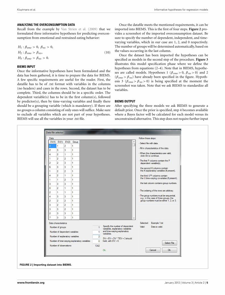
BIEMS INPUTOnce the informative hypotheses have been formulated and thedata has been gathered, it is time to prepare the data for BIEMS.A few specific requirements are useful for the reader. First, thedatafile has to be of .txt format with variables in the columns(no headers) and cases in the rows. Second, the dataset has to becomplete. Third, the columns should be in a specific order. Thedependent variable(s) has to be in the first column(s), followedby predictor(s), then by time-varying variables and finally thereshould be a grouping variable (which is mandatory). If there areno groups a column consisting of only ones will suffice. Make sureto exclude all variables which are not part of your hypotheses.BIEMS will use all the variables in your .txt file.

Once the datafile meets the mentioned requirements, it can beimported into BIEMS. This is the first of four steps. Figure 2 pro-vides a screenshot of the imported overconsumption dataset. Besure to specify the number of dependent, independent, and time-varying variables, which in our case are 1, 2, and 0 respectively.The number of groups will be determined automatically, based onthe values occurring in the last column.

Once the dataset has been imported the hypotheses can bespecified as models in the second step of the procedure. Figure 3illustrates this model specification phase where we define thehypotheses from equations (2–4). Note that in BIEMS, hypothe-ses are called models. Hypotheses 1 (βemo > 0, βres > 0) and 2(βemo > βres) have already been specified in the figure. Hypoth-esis 3 (βemo > βres > 0) is being specified at the moment thescreenshot was taken. Note that we ask BIEMS to standardize allvariables.

BIEMS OUTPUTAfter specifying the three models we ask BIEMS to generate adefault prior. Once the prior is specified, step 4 becomes availablewhere a Bayes factor will be calculated for each model versus itsunconstrained alternative. This step does not require further input

FIGURE 2 | Importing dataset into BIEMS.

www.frontiersin.org January 2012 | Volume 3 | Article 2 | 5

Kluytmans et al. Informative hypotheses for regression models

FIGURE 3 | Specifying hypothesis 3 in BIEMS.

from the user. Figure 4 displays the output screen of BIEMS. TheBayes factor for every model against its unconstrained alternativeis displayed. For every hypothesis a more detailed output filecan be obtained where, among many other statistics, the fit, andcomplexity can be found.

For H 1 – which stated that both predictors were positivelyrelated to overconsumption – we find a complexity of 0.250, afit of 1, and a resulting Bayes factor of 4.00. This means thatthe hypothesis in equation (2) receives four times more supportfrom the data than an unconstrained (empty) model does. H 2 –stating that emotional eating is more important for predictingoverconsumption than restrained eating – has a complexity of0.500, a fit of 1 as well, and consequently receives a Bayes factorof 2.00. This indicates that H 2 is still a better model for the datathan its unconstrained alternative. Finally, H 3 – which stated thatβemo > βres > 0 has a complexity of 0.125, a fit of 0.96, and a Bayesfactor of 8.04. This indicates that H 3 is eight times more likelythan the empty model it was compared to.

Recall that we were not merely interested in the hypothesesthemselves; we wanted to compare them and select the most opti-mal hypothesis for the data. As discussed in the intermezzo we

can obtain Bayes factors for the comparison of two hypotheses bydividing the Bayes factors of those hypotheses against an uncon-strained alternative. For example, comparing the Bayes factor ofH 3 with that of H 2 gives a Bayes factor of 8.04/2.00 = 4.02 and H 3

versus H 1 results in a Bayes factor of 8.04/4.00 = 2.01. This indi-cates that H 3 receives most support from the data, either whenit is being compared to an empty model or another informativehypothesis. To conclude, we would say that both emotional andrestrained eating are related to overconsumption with emotionaleating being the strongest predictor of the two.

ANALYZING THE WORK-FAMILY INTERFERENCE DATAFor the second analysis – predicting work-family interference fromcontractual hours and overtime hours – we again prepared thedata file and obtained Bayes factors for all three models. Recall ourinformative hypotheses from the introduction:

H1 : βover > 0, βcontr > 0,

H2 : βover > βcontr ,

H3 : βover > βcontr > 0.

(11)

Frontiers in Psychology | Quantitative Psychology and Measurement January 2012 | Volume 3 | Article 2 | 6

Kluytmans et al. Informative hypotheses for regression models

FIGURE 4 | BIEMS output screen.

The Bayes factor for H 1 against the unconstrained hypoth-esis is 4.05. For H 2 it is 1.73 and for H 3 it is 6.95. Althoughall informative hypotheses receive more support from the datathan their unconstrained alternatives do, H 3 fits the data best.Our conclusion would be that contractual hours and overtimehours are both related to work-family interference, but the rela-tion is stronger for overtime hours. A causal interpretation of theresults remains complicated because this research project was nota controlled experiment.

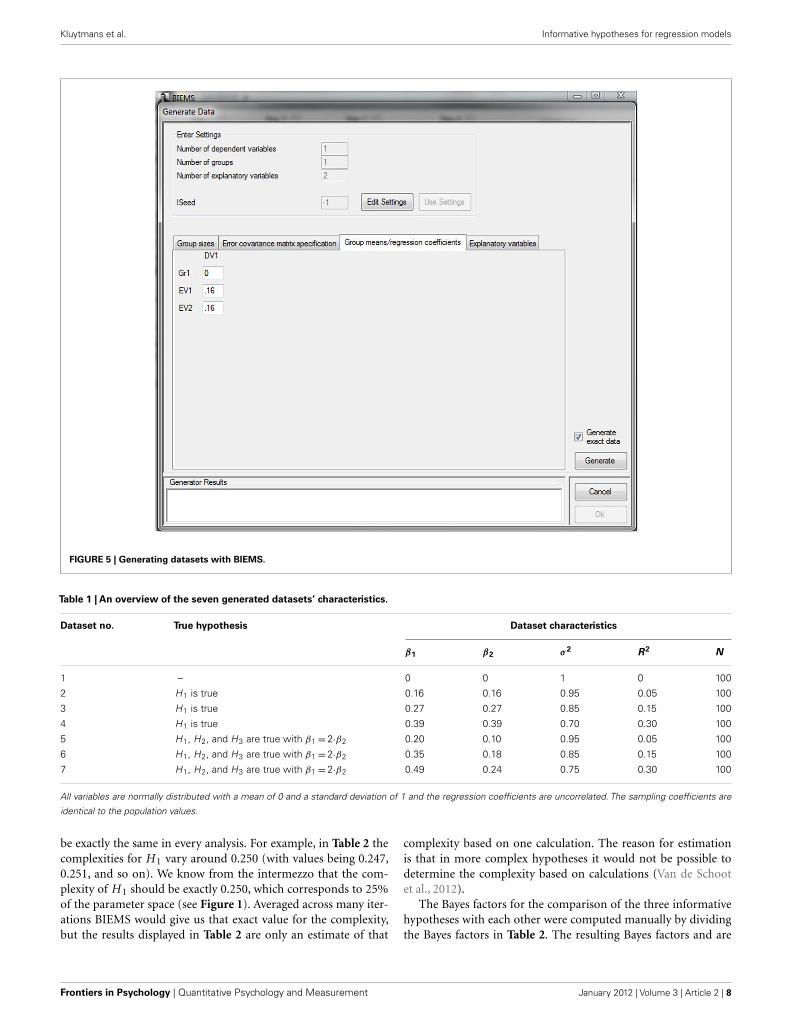
GENERATED DATASETS: VARIOUS EFFECT SIZESAs mentioned earlier we also want to demonstrate how theBayesian output is affected by differences in effect size. The pur-pose is to gather insight into the effect R2 has on the Bayesfactor (a concept that will be discussed in the next section).This influence has never been studied before in regression mod-els. Although our study is not extensive enough to serve as afull overview, it does give the reader a feeling of how effect sizeaffects the statistical output. In contrast to the real-world datasets,the generated datasets consist of 100 observations each. Thismakes them more comparable to certain areas of psychologicalresearch where smaller datasets are common, such as experimentalpsychology.

We determine the influence of R2 by generating seven datasetsthat have different β values and therefore different values for R2.

Table 1 displays the exact design of the seven datasets. All datasetswere generated with the DataGen function of the software packageBIEMS. Figure 5 provides a screenshot of the generation of dataset2 (see Table 1 for the corresponding βs).

The hypotheses we want to evaluate for these seven datasets area generalized form of the hypotheses outlined in the real-worldexamples:

H1 : β1 > 0, β2 > 0,

H2 : β1 > β2,

H3 : β1 > β2 > 0.

(12)

Because we exerted full control over the parameter values weknow which hypothesis describes which dataset best (see Table 1).For example, we know that if β1 > β2 then H 1 is not the besthypothesis for the data. We also know that in the first dataset,whereboth βs are zero, none of our informative hypotheses describe thedata well. This helps us judge the performance of our Bayesianmethod.

We evaluated the three informative hypotheses in equation (10)in the same way as the screenshots for the overconsumption dataillustrate. The fit, complexity, and Bayes factor for each hypoth-esis against an unconstrained hypothesis are reported in Table 2.Note that BIEMS estimates the complexity and due to the esti-mation process, the complexity for the three hypotheses will not

www.frontiersin.org January 2012 | Volume 3 | Article 2 | 7

Kluytmans et al. Informative hypotheses for regression models

FIGURE 5 | Generating datasets with BIEMS.

Table 1 | An overview of the seven generated datasets’ characteristics.

Dataset no. True hypothesis Dataset characteristics

β1 β2 σ 2 R2 N

1 – 0 0 1 0 100

2 H1 is true 0.16 0.16 0.95 0.05 100

3 H1 is true 0.27 0.27 0.85 0.15 100

4 H1 is true 0.39 0.39 0.70 0.30 100

5 H1, H2, and H3 are true with β1 = 2·β2 0.20 0.10 0.95 0.05 100

6 H1, H2, and H3 are true with β1 = 2·β2 0.35 0.18 0.85 0.15 100

7 H1, H2, and H3 are true with β1 = 2·β2 0.49 0.24 0.75 0.30 100

All variables are normally distributed with a mean of 0 and a standard deviation of 1 and the regression coefficients are uncorrelated. The sampling coefficients are

identical to the population values.

be exactly the same in every analysis. For example, in Table 2 thecomplexities for H 1 vary around 0.250 (with values being 0.247,0.251, and so on). We know from the intermezzo that the com-plexity of H 1 should be exactly 0.250, which corresponds to 25%of the parameter space (see Figure 1). Averaged across many iter-ations BIEMS would give us that exact value for the complexity,but the results displayed in Table 2 are only an estimate of that

complexity based on one calculation. The reason for estimationis that in more complex hypotheses it would not be possible todetermine the complexity based on calculations (Van de Schootet al., 2012).

The Bayes factors for the comparison of the three informativehypotheses with each other were computed manually by dividingthe Bayes factors in Table 2. The resulting Bayes factors and are

Frontiers in Psychology | Quantitative Psychology and Measurement January 2012 | Volume 3 | Article 2 | 8

Kluytmans et al. Informative hypotheses for regression models

Table 2 | Results corresponding to the generated datasets: Bayes factors for each informative hypothesis against its unconstrained alternative.

Dataset Bayes factor

f 1,u c1,u BF 1,u f 2,u c2,u BF 2,u f 3,u c3,u BF 3,u

1 0.25 0.247 1.01 0.50 0.49 1.01 0.12 0.12 0.99

H1 ISTRUE

2 0.88 0.251 3.56 0.49 0.503 0.99 0.44 0.124 3.51

3 0.99 0.250 3.90 0.49 0.499 1.00 0.49 0.124 3.97

4 0.99 0.251 3.95 0.50 0.498 1.01 0.49 0.125 3.96

H1, H2, AND H3 ARETRUE WITH β1 = 2·β2

5 0.81 0.252 3.29 0.73 0.500 1.50 0.58 0.126 4.66

6 0.96 0.247 3.84 0.88 0.500 1.76 0.84 0.125 6.62

7 0.99 0.250 3.93 0.96 0.496 1.90 0.94 0.126 7.60

Table 3 | Bayes factors for the comparison of the informative

hypotheses with one another.

Dataset Bayes factor

BF 12 BF 13 BF 23

1 1.00 1.02 1.02

H1 ISTRUE

2 3.59 1.01 0.28

3 3.90 0.98 0.25

4 3.91 0.99 0.25

H1, H2, AND H3 ARETRUE

5 2.19 0.71 0.32

6 2.18 0.58 0.26

7 2.07 0.52 0.25

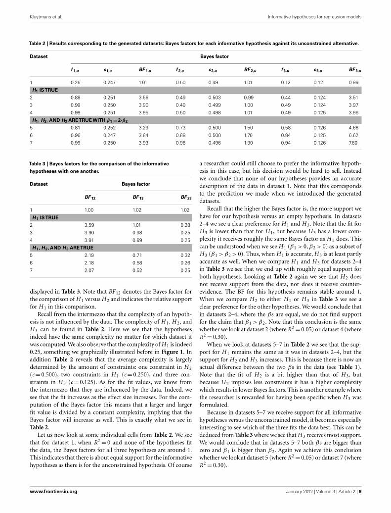
displayed in Table 3. Note that BF 12 denotes the Bayes factor forthe comparison of H 1 versus H 2 and indicates the relative supportfor H 1 in this comparison.

Recall from the intermezzo that the complexity of an hypoth-esis is not influenced by the data. The complexity of H 1, H 2, andH 3 can be found in Table 2. Here we see that the hypothesesindeed have the same complexity no matter for which dataset itwas computed. We also observe that the complexity of H 1 is indeed0.25, something we graphically illustrated before in Figure 1. Inaddition Table 2 reveals that the average complexity is largelydetermined by the amount of constraints: one constraint in H 2

(c = 0.500), two constraints in H 1 (c = 0.250), and three con-straints in H 3 (c = 0.125). As for the fit values, we know fromthe intermezzo that they are influenced by the data. Indeed, wesee that the fit increases as the effect size increases. For the com-putation of the Bayes factor this means that a larger and largerfit value is divided by a constant complexity, implying that theBayes factor will increase as well. This is exactly what we see inTable 2.

Let us now look at some individual cells from Table 2. We seethat for dataset 1, when R2 = 0 and none of the hypotheses fitthe data, the Bayes factors for all three hypotheses are around 1.This indicates that there is about equal support for the informativehypotheses as there is for the unconstrained hypothesis. Of course

a researcher could still choose to prefer the informative hypoth-esis in this case, but his decision would be hard to sell. Insteadwe conclude that none of our hypotheses provides an accuratedescription of the data in dataset 1. Note that this correspondsto the prediction we made when we introduced the generateddatasets.

Recall that the higher the Bayes factor is, the more support wehave for our hypothesis versus an empty hypothesis. In datasets2–4 we see a clear preference for H 1 and H 3. Note that the fit forH 3 is lower than that for H 1, but because H 3 has a lower com-plexity it receives roughly the same Bayes factor as H 1 does. Thiscan be understood when we see H 1 (β1 > 0, β2 > 0) as a subset ofH 3 (β1 > β2 > 0). Thus, when H 1 is accurate, H 3 is at least partlyaccurate as well. When we compare H 1 and H 3 for datasets 2–4in Table 3 we see that we end up with roughly equal support forboth hypotheses. Looking at Table 2 again we see that H 2 doesnot receive support from the data, nor does it receive counter-evidence. The BF for this hypothesis remains stable around 1.When we compare H 2 to either H 1 or H 3 in Table 3 we see aclear preference for the other hypotheses. We would conclude thatin datasets 2–4, where the βs are equal, we do not find supportfor the claim that β1 > β2. Note that this conclusion is the samewhether we look at dataset 2 (where R2 = 0.05) or dataset 4 (whereR2 = 0.30).

When we look at datasets 5–7 in Table 2 we see that the sup-port for H 1 remains the same as it was in datasets 2–4, but thesupport for H 2 and H 3 increases. This is because there is now anactual difference between the two βs in the data (see Table 1).Note that the fit of H 2 is a bit higher than that of H 3, butbecause H 2 imposes less constraints it has a higher complexitywhich results in lower Bayes factors. This is another example wherethe researcher is rewarded for having been specific when H 3 wasformulated.

Because in datasets 5–7 we receive support for all informativehypotheses versus the unconstrained model, it becomes especiallyinteresting to see which of the three fits the data best. This can bededuced from Table 3 where we see that H 3 receives most support.We would conclude that in datasets 5–7 both βs are bigger thanzero and β1 is bigger than β2. Again we achieve this conclusionwhether we look at dataset 5 (where R2 = 0.05) or dataset 7 (whereR2 = 0.30).

www.frontiersin.org January 2012 | Volume 3 | Article 2 | 9

Kluytmans et al. Informative hypotheses for regression models

The generated datasets were designed to demonstrate how R2

influences the results of Bayesian statistics. After having seen theseresults we would say that even when effect size is zero or relativelylow the Bayes factor helps us choose an accurate model for thedata. We conclude that the Bayes factor can be used even when theresearcher expects a small effect.

DISCUSSION AND CONCLUSIONIn this paper we have illustrated how informative hypothesescan be evaluated by means of Bayesian statistics. We applied themethod to existing psychological research, where we showed thereader the process of formulating informative hypotheses, evalu-ating them in light of the data, and interpreting the outcomes. Inaddition to this application we generated and analyzed datasetswith manipulated differences in effect size. This endeavor demon-strated how the Bayes factor was or was not affected by themagnitude of an effect. We now review our findings and discuss thepractical value of Bayesian hypothesis evaluation for psychologicalresearchers.

In the introduction we claimed that the null hypothesis isoften not the expectation that a psychological researcher wishesto evaluate. Instead we argued that researchers often have veryspecific prior expectations about parameter values. In the real-world examples for overconsumption and work-family inter-ference we saw that this was indeed the case: researchers hadprior expectations about the direction and magnitude of theeffects. We formulated these prior expectations and put them inthe form of informative hypotheses. We then pursued to eval-uate these hypotheses and express support for or against them.We were able to point out which hypothesis fit the data bestwithout having used any null hypothesis. Moreover, we pro-vided the reader with a step-by-step guide to enable him to dothe same.

From the generated datasets we saw that the Bayes factor helpsus select one of three models even when effect sizes are relativelylow. We also saw that the Bayes factor increased when effect sizedid, reflecting more and more certainty about the parameter val-ues as the magnitude of the effect increased. The tables in whichwe summarized the statistics will help the reader decide whetherthe approach is appealing enough for the effect sizes he/she isexpecting.

In sum, we have provided the reader with a non-technicalintroduction to Bayesian hypothesis evaluation while avoidingtechnical or mathematical language. Unfortunately there are somelimitations to this paper. For example, we have chosen artifi-cially simple designs with only two predictors and one crite-rion each. We acknowledge that the reader will likely be con-fronted with more complex designs in practice. For informativehypothesis testing in structural equation modeling, for example,please consult Van de Schoot et al. (2012). Second, our gener-ated datasets were nowhere near exhaustive. It would have beenmore thorough to also vary sample size. Third, we made a con-scious choice to omit mathematical formulas or calculations. Thismeans that the reader should either trust our intuitive expla-nations or read further into the method. For technical detailsof our proposed methodology we refer the interested reader to

Mulder et al. (2010). Fourth, we deliberately chose not to makethis paper a comparison between null hypothesis testing and theBayesian evaluation of informative hypotheses. For such com-parisons we refer the reader to Kuiper and Hoijtink (2010) orVan de Schoot et al. (2011a). Moreover, we chose not to providethe reader with any guidelines or cut-off values to interpret theBayesian output. This may seem unfriendly, especially because weexpect the reader to be a novice. Although we had good reasonsto exclude comparisons and cook-book rules, we acknowledgethat the lack of both may have been hard on the reader. Formore details on interpreting the Bayes factor see Kass and Raftery(1995).

In the introduction we promised to get back to the subject ofcontrast testing. We then acknowledged that contrast testing is aflexible tool to evaluate one informative hypothesis. Neverthelesswe still maintain that there are two important reasons for switchingto Bayesian hypothesis evaluation.

First, contrast testing only allow the evaluation of one singleinformative hypothesis. It does not provide an option for compar-ing competing hypotheses, which is essentially what model selec-tion is about. The Bayesian evaluation of informative hypothesisdoes allow the simultaneous evaluation of multiple informativehypothesis and, as we have demonstrated, assists the researcher inselecting one hypothesis from a set of hypotheses.

Second, although there is nothing wrong with null hypoth-esis testing, the philosophy behind Bayesian hypothesis evalu-ation may simply be more interesting to some researchers. InBayesian statistics the focus is on updating the state of knowl-edge: we quantified what we knew about parameters before wesaw any data and we updated this quantity after having seenthe data. The knowledge one gathers from one Bayesian analy-sis may serve as background knowledge for the next, creating anaccumulative science. In addition, Bayesian statistics focus on thesupport for a model rather than on p-values. This brings withit an entirely different line of interpreting and thinking aboutstatistics.

Of course there are certain situations in which the evaluation ofinformative hypotheses is not optimal. For example, a researchermay find himself truly interested in the null hypothesis (Wainer,1999). Note that in this situation the researcher may still choosebetween Bayesian and frequentist statistics as both frameworkscan handle null hypotheses. The choice will then likely be deter-mined by which framework’s philosophy is most appealing to theresearcher.

To conclude, we hope to have awakened some interest andawareness in the reader. We would advise the curious readerto become acquainted with informative hypotheses and theirBayesian evaluation through experimentation and literature. TheBayesian hypothesis evaluation we illustrated may not replace nullhypothesis testing entirely, but it may be a welcome addition to aresearcher’s toolbox.

ACKNOWLEDGMENTSWe thank our reviewers for their inspiring and constructive com-ments. Supported by a grant from the Dutch organization forscientific research: NWO-VICI-453-05-002.

Frontiers in Psychology | Quantitative Psychology and Measurement January 2012 | Volume 3 | Article 2 | 10

Kluytmans et al. Informative hypotheses for regression models

REFERENCESBerger, J. (1985). Statistical Decision

Theory and Bayesian Analysis, 2ndEdn. New York: Springer-Verlag.

Cohen, J. (1994). The earth is round(p<0.05). Am. Psychol. 49, 997–1003.

Cronbach, L. J. (1951). Coefficient alphaand the internal structure of tests.Psychometrika 16, 297–334.

Geurts, S., Beckers, D., Taris, T., Kom-pier, M., and Smulders, P. (2009).Worktime demands and work-family interference: does worktimecontrol buffer the adverse effects ofhigh demands? J. Bus. Ethics 84,229–241.

Hoijtink, H. (2012). InformativeHypotheses: Theory and Practice forthe Behavioral and Social Scientists.New York: CRC-press.

Hoijtink, H., Klugkist, I., and Boelen,P. A. (2008). Bayesian Evaluation ofInformative Hypotheses. New York:Springer.

Kass, R. E., and Raftery, A. E. (1995).Bayes factors. J. Am. Stat. Assoc. 90,773–795.

Klugkist, I., Laudy, O., and Hoi-jtink, H. (2005). Inequality con-strained analysis of variance: aBayesian approach. Psychol. Methods10, 477–493.

Klugkist, I., Van Wesel, F., and Bullens, J.(2011). Do we know what we test anddo we test what we want to know?Int. J. Behav. Dev. 35, 550–560.

Krueger, J. I. (2001). Null hypothesis sig-nificance testing: on the survival ofa flawed method. Am. Psychol. 56,16–26.

Kuiper, R. M., and Hoijtink, H.(2010). Comparisons of means

using exploratory and confirmatoryapproaches. Psychol. Methods 15,69–86.

Lynch, S. (2007). Introduction to AppliedBayesian Statistics and Estimationfor Social Scientists. New York:Springer.

Mulder, J., Hoijtink, H., and de Leeuw,C. (in press). BIEMS: a fortran90 program for calculating Bayesfactor for inequality and equal-ity constrained models. J. Stat.Softw.

Mulder, J., Hoijtink, H., and Klugkist, I.(2010). Equality and inequality con-strained multivariate linear mod-els: objective model selection usingconstrained posterior priors. J. Stat.Plan. Inference 4, 887–906.

Mulder, J., Klugkist, I., Van de Schoot,R., Meeus, W., Selfhout, M., andHoijtink, H. (2009). Bayesian modelselection of informative hypothesesfor repeated measurements. J. Math.Psychol. 53, 530–546.

Rosenthal, R., Rosnow, R., and Rubin,D. (2000). Contrasts and Effect Sizesin Behavioral Research: A Correla-tional Approach. Cambridge: Cam-bridge University Press.

Silvapulle, M. J., and Sen, P. K.(2004). Constrained Statistical Infer-ence: Order, Inequality, and ShapeConstraints. Series in Probability andStatistics. London: John Wiley Sons.

Silvapulle, M. J., Silvapulle, P., andBasawa, I. V. (2002). Tests againstinequality constraints in semipara-metric models. J. Stat. Plan. Inference107, 307–320.

Van de Schoot, R., Hoijtink, H., andDekovic, M. (2010). Testing inequal-

ity constrained hypotheses in SEMmodels. Struct. Equ. Modeling 17,443–463.

Van de Schoot, R., Hoijtink, H.,Hallquist, M. N., and Boelen,P. A. (2012). Bayesian evalua-tion of inequality-constrainedhypotheses in SEM models usingMplus. Struct. Equ. Modeling (inpress).

Van de Schoot, R., Hoijtink, H., Mul-der, J., van Aken, M., Orobio deCastro, B., Meeus, W., and Romeijn,J. (2011a). Evaluating expectationsabout negative emotional statesof aggressive boys using Bayesianmodel selection. Dev. Psychol. 47,203–212.

Van de Schoot, R., Mulder, J., Hoi-jtink, H., van Aken, M. A. G. ,Dubas, J. S., de Castro, B. O.,Meeus, W., and Romeijn, J.-W.(2011b). Psychological functioning,personality and support from fam-ily: an introduction Bayesian modelselection. Eur. J. Dev. Psychol. 8,713–729.

Van de Schoot, R., Romeijn, J.-W.,and Hoijtink, H. (2011c). Mov-ing beyond traditional null hypoth-esis testing: evaluating expecta-tions directly. Front. Psychol. 2:24.doi:10.3389/fpsyg.2011.00024

Van de Schoot, R., and Strohmeier,D. (2011). Testing informativehypotheses in SEM increases power:an illustration contrasting classicalhypothesis testing with a parametricbootstrap approach. Int. J. Behav.Dev. 35, 180–190.

Van Strien, T., Herman, C. P., andVerheijden, M. W. (2009). Eating

style, overeating, and overweight ina representative Dutch sample. Doesexternal eating play a role? Appetite52, 380–387.

Wagenmakers, E.-J. (2007). A practicalsolution to the pervasive problemsof p values. Psychon. Bull. Rev. 14,779–804.

Wainer, H. (1999). One cheer for nullhypothesis significance testing. Psy-chol. Methods 4, 212–213.

Conflict of Interest Statement: Theauthors declare that the research wasconducted in the absence of any com-mercial or financial relationships thatcould be construed as a potential con-flict of interest.

Received: 02 June 2011; accepted: 04 Jan-uary 2012; published online: 20 January2012.Citation: Kluytmans A, Van de SchootR, Mulder J and Hoijtink H (2012)Illustrating Bayesian evaluation ofinformative hypotheses for regressionmodels. Front. Psychology 3:2. doi:10.3389/fpsyg.2012.00002This article was submitted to Frontiersin Quantitative Psychology and Measure-ment, a specialty of Frontiers in Psychol-ogy.Copyright © 2012 Kluytmans, Van deSchoot, Mulder and Hoijtink. This is anopen-access article distributed under theterms of the Creative Commons Attribu-tion Non Commercial License, which per-mits non-commercial use, distribution,and reproduction in other forums, pro-vided the original authors and source arecredited.

www.frontiersin.org January 2012 | Volume 3 | Article 2 | 11