Using a Spreadsheet Simulation to Test Hypotheses About ...

Tested Studies for Laboratory TeachingProceedings of the Association for Biology Laboratory EducationVol. 36, Article 12, 2015

1

Using a Spreadsheet Simulation to Test HypothesesAbout Genetic Drift and SelectionRobert J. Kosinski

Clemson University, Department of Biological Sciences, 132 Long Hall, Clemson SC 29634-0314 USA ([email protected])

This exercise uses physical simulations, numerical simulations, and integrated statistical tests to allow students to explore a wide variety of population genetics topics. After a coin-flipping simulation, students use an elaborate Excel spreadsheet that allows both large-population (deterministic) and small-population (stochastic) simulations of allele frequencies. An unusual feature is that the spreadsheet has three kinds of built-in chi-square tests. The class is divided into groups, and all members of the same group perform replicate simulations. This allows both individual and group tests of hypotheses. Effects that may not be significant individually may be significant when group results are considered.

FirstpageKeywords: population genetics, evolution, Hardy-Weinberg equilibrium, Excel, simulation, genetic drift

© 2015 Clemson University

In this exercise, the students use a spreadsheet simula-tion to investigate the persistence time of both alleles at a two-allele locus as affected by population size, unselective mortality, and several kinds of selection. Three kinds of chi-square tests allow the students to test hypotheses individu-ally and (using pooled data) in groups. This is a “dry-lab” exercise with no safety concerns. To reduce time required to do the simulation, if desired, the theoretical background for Hardy-Weinberg equilibrium can be covered in lecture.

The spreadsheet model includes both deterministic and stochastic models of allelic frequency dynamics. Students will experience the sharp difference between the steady, smooth deterministic model and the unpredictable stochas-tic models. The models will allow students to rapidly verify expected outcomes (such as the extinction of a deleterious allele), and may surprise them with other outcomes (such as the rapid extinction of alleles in small populations, the ability of a recessive deleterious allele to persist for many generations once it falls to a low frequency, and stabiliza-tion of allele frequencies by amazingly small heterozygote advantage).

Some simulations (such as predator-prey simulations) only have interesting results with a narrow range of param-

eter choices. That is not true here. The simulations are the embodiment of Hardy-Weinberg assumptions (such as ran-dom mating, no mutation, etc.). Even the simulations using selection maintain the Hardy-Weinberg rules except the one prohibiting selection. The only parameters used are mortality rates and population size. All the rest of the models’ behavior comes directly from the assumptions of the Hardy-Weinberg Principle and random numbers generated by Excel.

The statistical component is an important part of the exercise. Even though this is a “dry” lab, it still generates data that allow the testing of hypotheses. Students must choose appropriate treatments to compare, must gather data from numerous replicates within each treatment, and must test these data with recognized statistical tools provided in the spreadsheet. A very important lesson is that when a larg-er group pools their observations, a more sensitive test is possible. Therefore, the exercise directs students to perform individual simulations first, then to combine all the data in their group (e.g., a lab table) for the more powerful test of the hypothesis.

Introduction

mailto:[email protected]

2 Tested Studies for Laboratory Teaching

Kosinski

Student OutlineOverview

In this exercise, you will learn how to compute allelic frequencies, and will use a coin-flipping simulation to understand why allelic frequencies in small populations fluctuate randomly even when there is no selection. Then you will use a spread-sheet simulation to explore the role of genetic drift and selection in evolution. Because of random elements, no two simulations will turn out the same way. You will be able to use the simulation results to carry out statistical tests of evolutionary hypotheses.

Exercise A. Allelic FrequenciesObjective

• Learn how to compute allelic frequencies.

We can track the fortunes of a population by noting how the number of individuals rises and falls. However, if we aremore interested in the evolution of the population, it would be more productive to keep track of how the numbers of different alleles rise and fall. We track the abundance of an allele by a measure called the allelic frequency. Changes in allelic frequencies are the basis of an area of study called population genetics.

Say we are studying the B/b locus, and this locus has two alleles, B and b. The frequency of B is defined as the fraction of all the alleles at the B/b locus in a population that are B. For example, if the whole population has the Bb genotype, half the alleles at the B/b locus are B, and the frequency of B is 0.5. If 70% of the population is bb, 10% is Bb, and 20% is BB, we compute the frequency of B by reasoning that none of the bb alleles are B and only half of the Bb alleles are B:

Population 0.7 bb 0.1 Bb 0.2 BBFrequency of B = [B] = (0)(0.7) + (0.5)(0.1) + (1.0)(0.2) = 0.25Frequency of b = [b] = (1.0)(0.7) + (0.5)(0.1) + (0.0)(0.2) = 0.75

An allelic frequency can never get higher than 1.0 (at which point the allele is said to be “fixed”) and cannot get lower than 0 (at which point the allele is said to be “extinct”).

Evolution is a change in allelic frequencies. This change might be adaptive, as when natural selection gradually elimi-nates as harmful allele, or it might be neutral or even harmful, as when random fluctuations eliminate an allele, reducing the ability of the population to adapt to future changes in the environment.

ProcedureGiven: population 1 has 20% BB, 0% Bb, 80% bb

Frequency of B = ___________ because

Given: population 2 has 5% BB, 30% Bb, 65% bb

Frequency of B = ___________ because:

Proceedings of the Association for Biology Laboratory Education, Volume 36, 2015 3

Major Workshop: Drift and Selection Simulation

Exercise B. Hardy-Weinberg EquilibriumObjectives

• Learn the conditions under which evolution will not occur (Hardy-Weinberg equilibrium);• Learn the genotypic frequencies predicted when Hardy-Weinberg equilibrium prevails;• Assess populations for their deviation from these predicted genotypic frequencies.

In 1908, Godfrey Hardy and Wilhelm Weinberg imagined a population that was large, mated randomly, and had no se-lection, mutation, or migration. They showed mathematically that under these very restrictive conditions, allelic frequencies would not change and therefore evolution would not occur. While the conditions may be unrealistic, Hardy-Weinberg Equi-librium (HWE) is a useful concept because it is a no-evolution null hypothesis and departures from its conditions indicate that evolution might be occurring.

If Hardy-Weinberg equilibrium prevails and mating is indeed random, we can imagine that all the gametes are put in a blender and collide randomly with one another. This means that the fraction of zygotes that are BB, Bb, and bb can be computed by a contingency table similar to a Punnett square. If p is the frequency of B and q is the frequency of b, then random collisions between the gametes will produce the zygote frequencies below:

Table 1. Predictions of genotypic frequencies if Hardy-Weinberg equilibrium prevails.

[B] = p [b] = q

[B] = p [BB]= p2 [Bb] = pq

[b] = q [bB] = pq [bb] = q2

This predicts that in a world of truly random mating and no selection, the frequency of BB should be p2, the frequency of bb should be q2, and the frequency of Bb should be 2pq (because it is the sum of the “Bb” and “bB” cells in the table above).

ProcedureIn Exercise A, you computed the frequencies of B in population 1 and population 2. Because there are only two alleles,

[b] = 1 – [B]. Which of these two Exercise A populations, 1 or 2, is closer to the genotypic frequencies predicted by Hardy-Weinberg equilibrium?

Try answering this question by filling in the information below:

Population 1: [B] = p = ________ [b] = q = ________

Population 2: [B] = p = ________ [b] = q = ________

Then fill Table 2:


Kosinski

Table 2. Observed and predicted genotypic frequencies for two populations.

Pop. 1 [BB] [Bb] [bb]

Observed 0.20 0 0.80

Expected


Observed 0.05 0.30 0.65

Expected

Which of these two populations is closer to the genotypic frequencies predicted by Hardy-Weinberg equilib-rium?

Look at the population above that diverges from the Hardy-Weinberg expectations. If there really were ran-dom mating and no selection, why is this distribution of genotypes hard to explain? What kind of selection and/or nonrandom mating could explain these genotypic ratios?

Exercise C. Genetic Drift Due to Chance Mating OutcomesObjective

• Use a coin-flipping simulation in order to demonstrate why allelic frequencies can be expected to fluctuate due to chancemating outcomes.

Genetic drift is the change in allelic frequencies that results from random events such as mating outcomes and unselec-tive mortality. These forces are more powerful in smaller populations, and can radically change allelic frequencies. An analogy would be a coin toss. If 100 people tossed coins at the same time, the percentage of heads would fluctuate close to 50%. All heads or all tails would be very unlikely results. However, if only three people were tossing the coins, it would be impossible to have half heads and half tails, and it would be expected that the tosses would produce all heads or all tails relatively frequently. The same chance deviations from predicted frequencies occur for combinations of alleles. For example, say that a population consists of two individuals, both Bb. If these two parents have two offspring, the offspring might be Bb and Bb, or BB and Bb, or BB and bb, or bb and bb, etc. In most of these cases, [B] will fluctuate away from 0.5. It might even fluctuate to zero and be lost. You will have the opportunity to see this effect for yourself in a simple coin-flipping simulation.

Procedure1. Pair with another student. You and your partner represent a Bb x Bb mating pair, and will repeatedly create pairs of off-

spring by each flipping a coin twice.

2. If the coin of a parent comes up heads, that person contributes a B to the mating; if it comes up tails, the contribution isa b. The two Bb people stay Bb despite what their offspring are. For example, say the two Bb people flip coins and getheads and heads. Their first offspring is BB. If they get a heads and a tails on their second flip, their second offspring willbe Bb. However, on every flip, the “parents” will remain Bb and Bb.

3. Create five pairs of offspring and fill in Table 3 below. Mating “zero” is done for you to show you what you have to do.



Table 3. Genetic drift as a result of random mating outcomes.Mating Offspring 1 Offspring 2 [B] [b]

0 BB Bb 0.75 0.2512345

Did these random fluctuations ever cause the frequency of B to reach zero or 1.0?

If so, this would have caused extinction of either the B or b allele in this “population.” If the population were larger (say, 100 offspring per generation instead of two), do you think the chance of allele extinction or fixation would be greater or less? Why?

The Spreadsheet SimulationAs Exercise C makes clear, random mating outcomes will cause violent fluctuations in the allelic frequencies of a small

population, and will probably cause the rapid extinction of one of the alleles at a locus. Thus, genetic drift can cause drastic and permanent changes in allelic frequencies. This is usually a harmful change because it reduces genetic diversity.

Coin-flipping simulations will only take us so far, however. To explore more complex dynamics, larger populations, and many generations, we will need a numerical simulation. This exercise uses a spreadsheet simulation that you will run on your laptop. Not only does it have simulations of various population sizes and selection regimes, but it also allows you to test hy-potheses with built-in chi-square tests.

The spreadsheet has two kinds of simulation models—deterministic and stochastic. Deterministic models have no random elements and produce the same results every time they are run. Because the random elements in an allelic frequencies model are more powerful with small population sizes, it could be said that the deterministic model (with zero random effects) simulates an infinitely large population. Stochastic models have random elements and each simulation may differ in its details from other simulations. The stochastic models in simulate population sizes of 4, 20, 100, and 500 organisms. As the popula-tion size gets larger, the models produce qualitatively different results. There are even more striking differences between the stochastic models and the deterministic one.

A stochastic simulation always starts with population that is 50% BB and 50% bb. These organisms contribute their gam-etes to the random-mating “blender,” and zygotes are produced that randomly draw from this gamete pool. The distribution of zygotes will vary randomly around the HWE genotypic frequencies of p2,, 2pq, and q2 for BB, Bb, and bb, respectively. Some simulations will have selection, expressed as a mortality rate for each type of zygote. A random number uniformly distributed between 0 and 1 is generated for each zygote. If the number is higher than the mortality rate, the zygote grows up to be an adult. If the number is lower than the mortality rate, the zygote dies, its alleles are deleted from the pool, and it is randomly replaced by one of the surviving organisms. This replacement is another source of random effects in the model. All adults then contribute their gametes to the gamete pool again. All simulations run for 200 generations, although fewer generations might be plotted for the smaller populations.

As it runs, the simulation automatically tests the distribution of genotypes in each generation for deviation from the p2, 2pq, and q2 predictions of HWE. This usually shows that unless selection against certain genotypes is operating, there isn’t a significant deviation from the HWE ratios. Another chi-square test allows you to test simulations for different persistence times of both the B and b alleles. Persistence of both alleles is much shorter with a smaller population because either B or b tends to go extinct. A final chi-square test compares simulations for their qualitative outcomes (e.g., does a simulation end with both B and b still present, or has one of the alleles gone extinct?).

The following exercises allow you to investigate the effect of population size and differing patterns of mortality on allele persistence.


Kosinski

Exercise D. The Effect of Population Size on Allele PersistenceObjectives

• Learn to use the spreadsheet simulation;• Observe and explain the difference between the deterministic and stochastic simulations;• Learn to use the spreadsheet’s built-in chi-square median test;• Use the median test to compare persistence times of both alleles in small and large populations.

There will be no mortality and no selection in this series of simulations, so all effects will be caused by drift due to ran-dom mating outcomes, as in your coin-flipping simulation. Watch for the startling contrast between the results of the determin-istic simulations and the stochastic ones, especially for small population sizes.

Procedure1. Open the spreadsheet. If it says the file is already open, indicate that you want to open it again. Click on the “Pop = 100”

tab. Adjust the size of the Excel window until you can see the part of the screen in Figure 1.

2. To the left of the screen you’ll see a heavy, black, vertical line. There’s no need for you to change or worry about anythingto the left of this line. The area to the left of the line keeps track of the reproduction of the “organisms” in the simulation.You will be concerned only with the display area to the right of the line.

3. Look at the tabs along the bottom of the screen, and click on the “Pop Infinite” tab unless it is already selected. This isthe deterministic model, with no random effects.

4. Check to see that the yellow mortality boxes (top right of the screen) all have zeroes in them, and that the violet “InitialBB” box has a 0.5 in it:

This starts the simulation with 50% BB and 50% bb.

Figure 1. The portion of the screen that should be visible as you work with the simulation.



5. Find the pink “Run” box, probably with a zero in it. You run the simulation by entering any number into this box andpressing Return or Enter. The number you enter has no effect on the outcome.

6. The graph may not appear to change, but the simulation just ran for 200 generations. Now change the “Initial [BB]” inthe purple run box to some other decimal between zero and 1.0 and press Enter or Return. Change to another initial [BB]and press Enter or Return.

7. Summarize the rather simple behavior of the deterministic model. Specifically:

a) If there is no selection, does the frequency of B change? Does evolution (defined as a change in allelic frequencies)occur with this model?

b) Is there any equilibrium [B] to which the model “homes,” or does it just stay wherever you start it?

c) If there is no selection and the population is very large, do these unchanging allelic frequencies make sense?

8. Click on the “Pop = 100” tab. First check that the yellow mortality boxes all have zeroes in them. If not, fill them in withzeroes and press Enter or Return. Here, the [B] may “wander” due to genetic drift, but it still is not homing to any equi-librium value. Therefore, if it drifts to a low or high value, there is nothing to bring it back but random chance. If it driftstoo high, it will fix. If it drifts too low, it will go extinct. It is like a blind, randomly-moving robot wandering around nearthe edge of a cliff.

9. Take a look at the right graph, which shows the value of chi-square from comparison of the genotypic frequencies withthose predicted by HWE. The horizontal red line is chi-square for P = 0.05, and the green line is chi-square for P = 0.01.

a) Does it look as if these genotypic frequencies are mostly consistent with those predicted by HWE? Given the model,why does this make sense?

b) Important question: Despite your HWE answer above, is evolution occurring in this population of 100 organisms?If your answer is yes, what is causing it?

Figure 2. The controls of the deterministic simulation.


Kosinski

10. The great differences between the simple output of the infinite population model and the complex and variable outputof the “Pop = 100” model needs some explanation. A population of 100 is small enough so that random mating outcomes can have a big effect over many generations. When the “Pop = 100” model was run three times, the three varying curves on the left of Figure 3 were obtained; when it was run 15 times, the curves on the right of Figure 3 were produced. However, when all the curves in the right graph were averaged together to produce the average [B] for each generation, the curve on Figure 4 was obtained. Figure 4 should remind you of the deterministic “Pop Infinite” output, and should convince you that there is no significant bias in the model. Figure 4 would probably be similar to the output of a model with 1,500 organisms.

11. Click on the “Pop = 500” tab, then 20, then 4. Make sure that all the mortality rates are zeroes, and just look at thecurves that are already present. As the population gets smaller, is there a greater or a lesser tendency for the B allele to either fix or go extinct? We will investigate this rigorously in just a moment, but you should be able to see some patterns.

12. We will now do a test on the persistence of both the B allele and the b allele as influenced by population size. We willdo this with all population sizes. Starting with “Pop = 4,” write down the length of time that both the B and b alleles persisted (that is, the time before extinction of one of the alleles). You could read this from the graph, or you might look just to the right of the heavy, vertical black line, under the “Freq. of B” column, to see the last generation in which [B] is neither 0 nor 1 (4 generations in Figure 5). This is the “persistence time” for that simulation.

Figure 3. Three (left) and 15 (right) “Pop = 100” simulations.

Figure 4. The average [B] of the 15 simulations in 3 at each generation.



13. Record this persistence time in the table below. Then click on the “Pop = 20” tab, check that all the mortality rates are zeroes, and record the persistence time there. Continue on through “Pop = 100” and “Pop = 500,” filling in the first line of Table 4 with persistence times. If the simulation reached 200 with both alleles still present, record that the persistence time was 200 generations.

14. Run “Pop = 500” again, and record the persistence at each population size again. Continue doing this until you have filled up Table 4 with 10 persistence times at each population size. Don’t worry about the last three rows of Table 4; we are about to use a statistical program to fill those in.

Table 4. The number of generations of persistence for both the B and b alleles.

RunPopulation Size

4 20 100 500

1

2

3

4

5

6

7

8

9

10

Mean

Chi-Sq

P Value

Figure 5. Output showing B and b persisted for four generations before B fixed.


Kosinski

15. A statistical test called the chi-square median test will allow us to determine whether larger populations have longer persistence of both alleles. In this test, the program pools all the persistence times together, determines the median of the persistence time data set, and then examines where persistence times fall with reference to the median. If population size makes no difference, we would expect that each population size would have times both above and below the median. If size does make a difference, the persistence times of some population sizes would be mostly below the median and others would be above it. The chi-square median test is more fully explained in the Student Appendix.

16. Click on the “Chi-Square Median” tab. Select any cells that have numbers in them and select “Clear Contents” from the edit menu. Put in the data points you’ve collected. The four population sizes are the treatments. It doesn’t matter that there is room for five treatments and one column is left blank. A typical set of entered data might look like this:

17. To the right, you’ll see information on the mean persistence times of the four population sizes, and how many of them were above and below the median. The yellow square on the left center of that page shows the result:

The P value is the probability that the differences in persistence times were just due to chance. If the P value is less than 0.05, there was a statistically significant difference between the population sizes. This is certainly the case in this example.

18. Fill in the means, chi-square and P value in Table 4. Did you find a significant difference in your data? If so…

Important question: Why do small populations tend to have far lower persistence times of both alleles than larger populations do?

Why are small, isolated populations of endangered species at great risk for loss of their genetic diversity?

Figure 6. Data entry area of the chi-square median test spreadsheet.

Figure 7. Results section of the median test spreadsheet. It has a yellow background.



Exercise E. Understanding Chi-Square FluctuationsObjective

• Determine whether rare but large chi-square values for deviation from HWE genotypic ratios can be explained as random fluctuations.

The second graph in the display area of the spreadsheet plots the chi-square values for deviation of genotypic ratios from the p2, 2pq, and q2 values expected if the conditions of the Hardy-Weinberg Principle are satisfied (principally, random mating and no selection). These curves seem like white noise that periodically exceeds the significant chi-square values for 1 degree of freedom and P = 0.05 (red line) and P = 0.01 (green line):

Statistics such as chi-square can give significant results if there is a real difference between treatments, but they might also give a false significant result just due to chance deviations. When we set our significance level at 0.05, for example, we’re saying that we will declare a significant difference when the differences are sufficiently large that they would only occur by chance 5% of the time. However, this means we will falsely declare a significant difference in 5% of all tests. We will now see if we can explain these fluctuations by the theory that they are random events and that the number of times the red and green lines are exceeded can be predicted.

Procedure

1. Select the “Pop = 500” page because this population is sufficiently large so that an allele rarely goes extinct in the 200-generation time span of the graph. It seems that this population should fit the Hardy-Weinberg conditions. It is large, mating is random, and there is no mutation, selection, or migration. There is no force but chance that can cause deviation from the expected Hardy-Weinberg genotypic ratios.

2. Run the “Pop = 500” simulation and count the number of times the chi-square line exceeds the red line and the green line. If the chi-square curve touches a line, count that as well. If it exceeds the green line, it must exceed the red line as well. Fill in your values in Table 5.

Figure 8. A chi-square graph for a Pop = 500 simulation. The red line is exceeded 8 times and the green line is exceeded once in this simulation.


Kosinski

Table 5. Times chi-square exceeded the red line and the green line.

Your Data Class Average

Exceeded Red

Exceeded Green

3. The simulation ran for 200 generations. We would predict that 5% of the time (10 generations), chance alone would causethe chi-square value to exceed the red line, and 1% of the time (2 generations), it would exceed the green line. Your in-structor will poll the class and find the class average, which you should write in Table 5 as well.

How close did the class average come to the expected values of 10 and 2 per 200 generations?

Exercise F. The Effect of Unselective Mortality on Allele PersistenceObjectives

• Determine the lowest unselective morality rate that causes a significant difference in the fraction of simulations that endin the extinction of one of the alleles;

• Determine if severe but unselective mortality causes significant deviations from the genotypic ratios predicted by Hardy-Weinberg equilibrium.

Genetic drift is a random fluctuation in allelic frequencies. One major cause is random mating outcomes, as detailed above. Another cause is random mortality such as deaths caused by accidents. Recall that in the stochastic model, dead zygotes are replaced by living organisms. Even though the mortality is not causing consistent selection, this random replacement effect does intensify drift.

Procedure1. Start with the “Pop Infinite” model. Enter mortality rates of 0.5, 0.5, and 0.5 for the three genotypes. This mortality is

serious but unselective.

What happens? Why does this outcome make sense for an infinite population with no random influences?

2. Go to the “Pop = 100” model. This population size has some tendency for alleles to go extinct so we can use it to measureallele persistence times. Run several simulations with all mortality rates zero. Note the persistence times of both allelesand the size of the chi-square values on the right graph in relation to the red and green lines (the significant chi-squarevalues).

3. Now enter mortality rates of 0.5, 0.5, and 0.5. Run the simulation several times.

What effect does the mortality have on the ability of both alleles to persist in the population for the whole 200 generations?

4. Also, look at the right graph, which shows the chi-square values for deviation from HWE genotypic ratios.

Do they seem larger than in the zero mortality case? Why?

5. At this point, your instructor may assign several different mortality rates to different groups in the lab (for example, eachlab table will use a different rate). These should range from about 0.5 down to 0.1. Don’t start doing simulations yet, butusing the “Pop = 100” model, everyone at a table will do 20 simulations with zero mortality for all genotypes, and then20 more simulations in which all genotypes have the assigned mortality.

6. Recording persistence time will not be the best strategy here because there will be many ties at 200 generations. Insteadof recording persistence times, you should count the number of simulations that end in each of two conditions: either bothB and b are still present, or one of the alleles is extinct. The chi-square spreadsheet that uses these categories is found



at the tab “Chi-Square on B Fates.” The null hypothesis for this test is that the fraction of simulations in the control and the mortality groups that end with both B and b present are the same. There is more information on this chi-square test in the Appendix.

7. So, for example, say a lab table is assigned a mortality of 0.5. Each student would run 20 control simulations without anymortality and 20 simulations with all genotypes suffering a 0.5 mortality. Each student will record how many terminatedwith B fixed or extinct, and how many terminated with both B and b still present. Each student will perform an individualchi-square test on his or her 40 simulations. Remember, the mortality for all three genotypes should always be the same.

8. One of the important principles of statistics is that more observations allow the detection of smaller effects. For this rea-son, everyone in the group will add up their results for both the control and the mortality treatment. Say the results werethat out of 40 control simulations, 20 ended up with B fixed or extinct, and 20 ended with both B and b still “alive.” Thiswould be entered next to “Trt 1.” For the mortality simulations (“Trt 2”), these numbers were 10 and 30. The left side ofFigure 9 below shows the data entry on the “Chi-Square on B Fates” page, and the right shows the chi-square results—there was a significant difference between the two treatments because the P value was less than 0.05.

9. Now do your simulations. Enter your individual results as hash marks in Table 6. Perform the chi-square test in Figure 9and record your individual results on the last two rows of Table 6. When your group is finished doing their simulations,add up all their numbers and fill in the top four cells of Table 7. Perform the same chi-square test on these summed num-bers. Come to a conclusion about your mortality rate, and be ready to contribute to a class discussion about the lowestuniversal mortality rate that can create a significant difference in the fate of the alleles over 200 generations.

Your group’s assigned mortality rate____________

Table 6. Numbers of simulations (your individual results).

B & b Both Present One Allele Extinct

No Mortal-ity

Mortality

Chi-Sq.

P Value

Table 7. Numbers of simulations and statistical results (group)


No Mortality

Mortality

Chi-Sq.

P Value

Figure 9. Data entry and results for the sample unselective mortality results.


Kosinski

Natural SelectionSelection against a genotype occurs when its fitness (success at survival and reproduction) is not as great as the fitness

of another genotype. Some students believe that selective value lies with the allele, that there are certain superior alleles that increase in frequency, while the inferior alleles decrease. However, selection is usually against a genotype. So, for example, if a person has two mutated CFTR alleles, he or she has cystic fibrosis. However, people with only one mutated allele are carriers and have normal health, just like the individuals with no mutated CFTR allele. There is no selection against the mutated, reces-sive allele provided it is in a heterozygote.

Genotypes that have selection against them will slowly decrease in frequency until the deleterious alleles responsible disappear from the gene pool of the population. However, the situation may be more complicated than simple elimination. Much depends on the selective pressure against the affected genotypes and whether the harmful allele is dominant or recessive. If the heterozygote has a substantial advantage over both homozygotes, the persistence of both alleles in the population will be prolonged. If the homozygotes have an advantage over the heterozygote, the system may become unstable, leading to the rapid elimination of one of the alleles. The allele eliminated may not be the one whose homozygote has the lower fitness. The one eliminated may just be a matter of chance.

In the remaining exercises, you will use the simulation to explore selection against a genotype and heterozygote advan-tage as factors influencing the persistence of deleterious alleles in a population.

Exercise G. The Effect of Selection and Recessiveness on Persistence of Harmful AllelesObjectives

• Observe the effect of selective mortality on the persistence of a harmful allele;• Contrast the different rates of elimination when the allele is recessive, incompletely dominant, or completely dominant.

In this exercise, you will assume that the b allele has a deleterious effect on survival, either just on the bb genotype (asin cystic fibrosis) or on both the bb and the Bb genotypes. In other words, we will test a recessive harmful b allele vs. an in-completely dominant one vs. a completely dominant one. Because the noise of genetic drift can obscure the effects we wish to examine, we will work with the “Pop Infinite” simulation in this exercise.

Procedure1. Go to the “Pop Infinite” simulation and enter that BB will start with a genotypic frequency of 0.5. Then enter 0.5 into the

yellow mortality box for bb, and make the other mortality rates zero. Run the simulation and see what happens. Keep in mind that the B allele is being graphed, so as the graph climbs higher, the b allele is being eliminated.

2. Leave the bb mortality rate at 0.5 and enter a mortality rate of 0.25 for Bb. How does this change affect the persistenceof the harmful b allele?

3. Leave the bb mortality rate at 0.5 and enter a rate of 0.5 for Bb as well. This simulates a completely dominant harmfulallele.

4. Repeat step 1, but use 0.1 as the mortality rate of bb and 0 for the other two rates (recessive b). Note how b seems to fallto a low level and then persist for a long time rather than being eliminated.

5. Repeat step 2, but use 0.1 and 0.05 as the mortality rates (incompletely dominant b).

6. Repeat step 3, but use 0.1 and 0.1 as the two mortality rates (completely dominant b).

First, what do you conclude about the relationship between the mortality rate a deleterious allele causes (e.g., 0.5 vs. 0.1) and its ability to persist in the population?

Second, what do you conclude about the relative persistence times of harmful alleles that are recessive, incompletely dominant, and completely dominant?

Explain why the great majority of rare, recessive deleterious alleles are present not in affected individu-als, but in asymptomatic “carriers.” For example, in cystic fibrosis, there are 100 times more carriers than people with the disease in the United States.



Exercise H. Heterozygote AdvantageObjectives

• Observe and explain the tendency of heterozygote advantage to prevent the extinction of the alleles in the advantaged hetero-zygote;

• Observe and explain the fact that populations with heterozygote advantage have equilibrium allelic frequencies to which thepopulation is attracted;

• Observe and explain the tendency of populations experiencing heterozygote advantage to depart strongly from predictedHardy-Weinberg genotypic frequencies;

• As a class, determine the smallest heterozygote advantage that can significantly prolong the existence of both alleles of aheterozygote.

Another way in which alleles are preserved is if heterozygotes have a selective advantage over both of the homozygotes (as-suming that only two alleles are possible at a locus). This is sometimes called “overdominance.” In a population in which heterozy-gotes are the most abundant and successful organisms, both alleles must be preserved. A classic example of heterozygotes advantage is the persistence of sickle-cell anemia in equatorial Africa. Sickle-cell anemia is a severe blood disease present in ss individuals. Ss individuals have some mild sickle-cell symptoms, but they are also resistant to malaria. Finally, normal (SS) individuals are not anemic at all but may suffer disability or death if they become infected with malaria. In areas of Africa where malaria is prevalent, heterozygotes seem to have a selective advantage over normal individuals, which seems to preserve the sickle-cell allele in the gene pool. However, in areas where malaria is not common, Ss individuals have no advantage and the sickle-cell allele is eliminated.

Heterozygote advantage is also theoretically interesting because it can cause allelic frequencies to converge on an equilibrium density, no matter where they start. The fact that the population gravitates to this equilibrium from any starting point is the key factor preserving both alleles.

There is also a “homozygote advantage” (or “underdominance”), in which the outcome is dramatically different. Here the equilibrium exists but is unstable, and one allele or the other rapidly goes extinct.

Procedure1. Go to the infinite population model. Start the fraction of BB in the population at 0.5. Give the heterozygote a zero mortality

rate, but give the two homozygotes the same mortality rate (say 0.5). Run the model.

2. Now change the initial fraction of BB to either a low or high value, but not 0.0 or 1.0. Run the model.

Important Question: What do you observe? How is this different from what happened with zero mortality for all genotypes? Why do you think it is happening?

3. Make the homozygote mortality rates unequal, but both greater than the heterozygote mortality rate. Run the model.

How is this behavior different from the behavior in step 2?

4. Not only does heterozygote advantage create an equilibrium allelic frequency, but the degree of fluctuation is affected aswell. Go to the “Pop = 100” simulation. Make the mortality rate of both homozygotes some low number like 0.05. Leave theheterozygote mortality at zero. Run the simulation. Note both the degree of fluctuation and the size of the chi-square numbersin the right graph with respect to the red and green significance level lines.

5. Gradually increase the homozygote mortality.

What happens to the degree of fluctuation in the allelic frequency of B as you increase the mortality rate? In a population where, increasingly, only Bb organisms survive, why do the fluctuations diminish?


Kosinski

6. Look at the chi-square deviation values as you increase the homozygote mortality rates.

Allelic frequencies are probably not changing very much so why are the chi-square deviation values in-creasing?

7. We will now do a systematic investigation of how heterozygote advantage affects the qualitative outcome of simulations.We will follow the procedure used in the unselective mortality exercise. Using the “Pop = 100” model, each group (e.g.,table) will do multiple simulations using both all-zero mortality rates (the no-selection control) and mortality rates thatshow balanced heterozygote advantage (the experimental treatment). Each person will do 20 simulations for each treat-ment (40 in all), and then the table will pool their results in order to determine if the fate of B is significantly differentin the control and the heterozygote advantage treatment. We wish to determine the lowest mortality rate that will give asignificant effect.

8. Unless your instructor gives different directions, the different groups should use the following mortality regimes for theheterozygote advantage treatment (and mortalities of 0, 0, 0 for the control treatment):

BB Bb bb

0.1 0.0 0.10.05 0.0 0.050.02 0.0 0.020.01 0.0 0.010.005 0.0 0.005

If there aren’t enough groups to do all these, leave out the lines at the top; 0.1 is certain to show a heterozygote advan-tage effect.

9. Enter your individual results as hash marks in Table 8. Perform the “Chi-Square on B Fates” test and record your individ-ual results on the last two rows of Table 8. When your group is finished doing their simulations, add up all their numbersand fill in the top four cells of Table 9. Perform the same chi-square test on these summed numbers. Come to a conclusionabout your mortality rate, and be ready to contribute to a class discussion about the lowest homozygote mortality rate thatcan create a significant difference in the fate of the alleles over 200 generations.



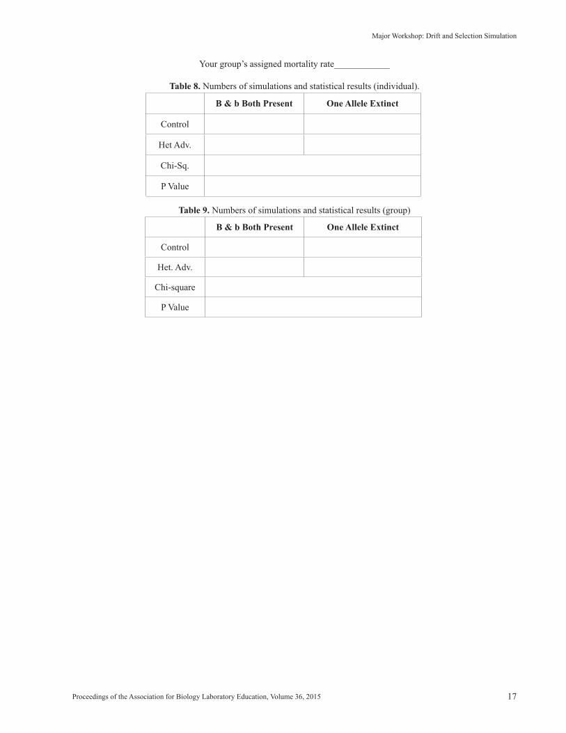
Your group’s assigned mortality rate____________

Table 8. Numbers of simulations and statistical results (individual).


Control

Het Adv.

Chi-Sq.

P Value

Table 9. Numbers of simulations and statistical results (group)


Control

Het. Adv.

Chi-square

P Value


Kosinski

Appendix to Student Outline: The Chi-Square TestsThe Role of Statistics

Say that you have measured the persistence times of both the B and b alleles under two selection regimes. Alleles in one treatment seemed to last longer than in the other treatment, but not by much. So what do you conclude? How big a difference between groups do we need before we reject the null hypothesis that the two selection situations give the same results? Giving assistance with this problem is the purpose of experimental statistics.

Statistics give us the probability of the observed difference between treatments if there were really no treatment effects. Put another way, statistics gives us the probability that the results are due to chance and not some real difference between the treatments. In biology, it is traditional to “fail to reject the null hypothesis” if this probability (the P value) is higher than 0.05 (5%). We say that 0.05 is our significance level, and that differences with a P value of less than 0.05 are “significant at the 0.05 level.” Therefore,

• if the P value is equal to or less than 0.05, we can reject the null hypothesis. This means we have evidence that thereis a difference between the treatments;

• if the P value is greater than 0.05, we cannot reject the null hypothesis. This means that we have no evidence that thereis a difference between the treatments.

These principles can be seen in one of the statistical tests we will use in this lab, the chi-square (c2) median test. This test is easy to understand and can be used in almost any situation in which two (or more) treatments are being compared.

The Chi-Square Median TestImagine that a series of simulations with no selection (A) and with weak selection (B) produce the following persistence

times of both alleles:

A: 120, 140, 160, 195, 109, 93, 110, 130, 101, 85 average = 124.3B: 114, 145, 165, 102, 200, 115, 95, 118, 91, 125 average = 127.0

Say that we pool these observations into one data set, order them from shortest persistence to the longest persistence (irrespective of treatment), and then code A observations as an “A” and B observations as a “B.” The shortest persistence was 85 generations (from A), so the first letter on our list should be an A. The next longest was 91 (from B), so the next letter will be a B. The longest time of all was 200, a B. The median of the pooled data set is 116.5. The median divides the data set into two parts. Half the observations will always be below the median and half above it. If we look at the number of As and Bs above and below the median, we see:

Table 10. Number of observations above and below the median for the A vs. B comparison.A B

Below Median 5 5Above Median 5 5

This is exactly the distribution of A and B observations above and below the median we would expect if the two sets of conditions produced the same persistence time.

On the other hand, let’s say we try some more severe selection (selection regime C) and when we compare A (no selec-tion) with C we find:

A: 120, 140, 160, 195, 109, 93, 110, 130, 101, 85 average = 124.3C: 75, 84, 85, 80, 80, 115, 98, 79, 82, 200, 125 average = 127.0

The median of the pooled data set is now 99.5 and if we look at the number of As and Cs above and below the median we see:



Table 11. The A vs. C comparison.A C

Below Median 2 8Above Median 8 2

If there were really no difference between the treatments, this very uneven distribution, with almost all A observations longer than the median persistence time and almost all C observations shorter than the median persistence time, would be very im-probable.

A statistic called chi-square (c2) can attach a probability to both the arrangements above. c2 contrasts the counts of ob-servations in classes (for example, above and below the median) with the counts expected if there were really no difference between the treatments. Statisticians have compiled extensive tables of how often c2 values of various sizes occur in simulated data where there is really no difference between the treatments.

The c2 and probability values associated with increasingly uneven distributions of two treatments (Trt 1 and Trt 2) with ten observations each are shown below. The probabilities shown are the probabilities that this distribution above and below the median could have originated just due to chance, not due to any real difference between the treatments. Note how the distribu-tions become more and more improbable (if due to chance alone) as they become more uneven.

Table 12. Chi-squares and P values for median tests with increasingly uneven distributions of observations.

Again, in biology, the traditional significance level is 0.05. We would say the last case above shows a significant differ-ence between Treatment 1 and Treatment 2 at the 0.05 level. The case above it does not because “0.05-0.10” is not equal to or less than 0.05.

Trt 1 Trt 2Below Median 5 5Above Median 5 5




c2 = 0Probability = 0.75-0.90

c2 = 0.8Probability = 0.25-0.50

c2 = 3.2Probability = 0.05-0.10

c2 = 7.2Probability = 0.005-0.01


Kosinski

Chi-Square Calculations in the Median Testc2 compares observed versus expected counts, and uses the formula

c2 = S[(O - E)2/E]

where O is the observed count, E is the expected count, and the S means summation over all classes. For example, in the A-B experiment and the A-C experiment, we have 10 observations per treatment and therefore we expect 5 observations in each treatment to be above the median and 5 to be below it. There are four classes (treatment A above and below the median, and treatment B above and below the median). Therefore, for the A vs. B experiment, c2 would be:

c2 = (5 - 5)2/5 + (5 - 5)2/5 + (5 - 5)2/5 + (5 - 5)2/5 = 0

For the A vs. C experiment, c2 would be

c2 = (2 - 5) 2/5 + (8 - 5) 2/5 + (2 - 5) 2/5 + (8 - 5) 2/5 = 7.2

The “B Fates” Chi-SquareAny simulation can only end two ways—either one of the alleles is extinct, or both are still present in the population. The

“B Fates” chi-square evaluates whether two treatments differ in the proportion of these two fates. It uses a contingency table chi-square.

Using the previous example, say that the control has 20 simulations that ended with one allele, and 20 that ended with two alleles. Say the experimental has 10 ending with one allele and 30 ending with two alleles. The contingency table would be:

Table 13. Observed numbers of observations in the B fates example.

One Allele Two Alleles Marginal Sums

Control 20 20 40Experimental 10 30 40

Marginal Sums 30 50 80

Looking at the marginal sums, note that overall 3/8 of the finishes had one allele and 5/8 had two alleles. This means that since there were 40 control simulations and 40 experimental simulations, if those two treatments were the same, 3/8 of the con-trols and 3/8 of the experimentals (15) should have been one-allele finishes, and 5/8 (25) should have been two-allele finishes. All the expected values would be either 15 or 25:

Table 14. Expected values (assuming the null hypothesis) for the B fates example.One Allele Two Alleles

Control 15 25Experimental 15 25

Using the formula c2 = S[(O - E)2/E] (above) and totaling over all cells of the table,c2 = 1.67 + 1 + 1.67 + 1 = 5.33

The degrees of freedom is (rows -1)(columns – 1) = 1. The observed Chi-squared value of 5.33 with 1 df is significant at the 0.05 level. The deviation between the observed and expected values is large enough so that we can reject the null hypothesis that the controls and experimentals had the same proportion of one-allele and two-allele finishes.



MaterialsEquipment Needed for a Class of 25

None, aside from coins for Exercise C and laptops for each student, presumably furnished by the students them-selves. I wrote the simulations in Excel because it is so uni-versally available to students. At least until the end of 2014 (and maybe after that), the spreadsheet (called “Drift-Selec-tion Spreadsheet”) can be downloaded from Clemson’s bi-ology majors lab site, <HTTP://biology.clemson.edu/bpc/bp/Lab/110/handouts.html>. It is found with the other ma-terial for the week of December 1. For the indefinite future, it can also be downloaded from HTTP://www.clemson.edu/~rjksn/ABLE/Drift-Selection.xlsx. The spreadsheet will be downloaded to your downloads folder or desktop. However, apparently this download is a read-only file, so to save it, you must give it another name such as “Drift-Selec-tion1.xlsx.”

Time and Background RequirementsAt Clemson, we will use this exercise in a laboratory

on evolution in an introductory biology course for majors. The students also do an analysis of some mitochondrial DNA data during the laboratory, so the exercise at Clemson does not take a whole period. However, our students are already familiar with the basic concepts of allelic frequencies and Hardy-Weinberg equilibrium from lecture, and they have used the chi-square median test several times already. If the preparation of your students is not as good, you could gain some time by leaving out Exercise E first, and jettisoning both Exercises E and F if you need even more time to fin-ish. This will leave out unselective mortality (not usually an important population genetics topic), but will still give full coverage to drift and selection.

Notes for the InstructorExercises A and B

Ideally, the students would cover allelic frequencies and Hardy-Weinberg equilibrium (HWE) in lecture before they did this laboratory. For this reason, Exercises A (com-puting allelic frequencies) and B (genotypic frequency pre-dictions of HWE) are short, merely a review. In both popu-lations in Exercise A, [B] = 0.2 and [b] = 0.8. The filled-in Table 2 should be:

Table 15. The correct answers for Table 2.


Observed 0.20 0 0.80

Expected 0.04 0.32 0.64


Observed 0.05 0.30 0.65

Expected 0.04 0.32 0.64

Obviously, Population 2 is much closer to the geno-typic frequencies predicted by Hardy-Weinberg equilibrium. In Population 1, it would be hard to explain how a population with random mating would have no heterozygotes. Perhaps in Population 1 there is selection pressure against the hetero-zygotes, or homozygotes preferentially mate with their own genotypes. The basic problem students sometimes have with these exercises is that they’re still thinking of genetics, and they think the genotypic ratio must be 1:2:1 or 3:1 or some other well-known genotypic ratio from a classic Mendelian cross.

Exercise C The experiment using the flipped coins can be confus-

ing because the students don’t understand that they are a pair of Bb organisms that are repeatedly generating pairs of off-spring. The main idea is that even when the parents stay the same, random assortment of maternal and paternal chromo-somes into gametes can create very different offspring, and this causes fluctuations in the frequencies of alleles.

The simulation exercises (Exercises D-G) should be easy for students to follow. Once they get proficient with the spreadsheet, they will be able to go through 20 simulations with astonishing speed. However, some exercises require the students to operate as a group, and then groups are asked to convene to reach a conclusion. The challenge for the instruc-tor is to keep the class together enough for these collabora-tive activities.

Exercise DIn the population size experiment, there is a sharp dif-

ference between the no-selection deterministic simulation results (left) and one example of the stochastic results using a population size of 100 (right):

The students might have a hard time believing that these two graphs represent the same system, but refer to Fig-ures 3 and 4, which show that many graphs like the one on the right do average precisely to the one on the left. The left graph is so steady because the zygotes of each genotype are

http://biology.clemson.edu/bpc/bp/Lab/110/handouts.html

http://biology.clemson.edu/bpc/bp/Lab/110/handouts.html

http://www.clemson.edu/~rjksn/ABLE/Drift-Selection.xlsx

http://www.clemson.edu/~rjksn/ABLE/Drift-Selection.xlsx


Kosinski

produced by multiplying allelic frequencies together (the fa-miliar p2, 2pq, and q2). As long as p and q do not change, the fraction of BB, Bb, and bb zygotes will be the same in every generation…which means that p and q and the genotypic fre-quencies will be the same in the next generation. Thus, it is understandable that the allelic frequencies in the left graph never change, and stay wherever they start.

In the right graph, zygotes are produced with a random element. Given the allelic frequencies, zygotes are produced by random selection of gametes. Before selecting each gam-ete, the programs asks if a rectangularly-distributed random number between 0 and 1 is less than p2, between p2 and p2 + 2pq, or greater than p2 + 2pq. One run of random numbers may produce more BB than it “should” in one generation, and more bb than it “should” in another generation. This random effect will be overpowering if the population is small. Refer the students back to Exercise C, the coin-flipping experiment. Also, the fact that there is no equilibrium point to which the allelic frequencies are attracted means that allelic frequencies wander in a true random walk.

In Exercise D, the students record individual data on allelic persistence, but there is no requirement for collabora-tion. This is to get them used to using the statistical program without the additional complication of collaboration. The chi-square median test is explained in the Appendix of the student outline.

Exercise EThe exercise involving chi-square fluctuations might

surprise students. Students often think that statistical tests can magically “see through” random variation and detect true dif-ferences. Actually, the tests can only compare the degree of variation between treatments with that expected due to ran-dom chance, and sometimes tests falsely declare differences that do not exist. This exercise asks students to compare the number of times the chi-square value for deviation from HWE genotypic ratios exceeds the P = 0.05 and P = 0.01 significance level with the number of times expected from chance alone.

The instructor then polls the class to find out how close the values from a 200-generation simulation come to the expect-ed values of 10 (5% of 200) and 2 (1% of 200). Because the “Pop = 500” simulation without selection is very close to a perfect Hardy-Weinberg machine, we would expect the ob-served and expected values would be very close. They are, but there are usually slightly more significant chi-squares than expected. In one series of 30 simulations, the average was 10.63 times for P = 0.05 value and 2.33 times for the P = 0.01 value. There is probably a non-random factor in the simulations that is causing large chi-squares, but most of the significant chi-squares are false positives caused by random events. This is a worthwhile lesson for anyone intending to test populations for deviation from Hardy-Weinberg expect-ed genotypic ratios.

A question to which I do not have a ready answer is why the chi-square that tests for deviations from HWE geno-typic ratios gets more and more significant as the unselective mortality rate increases. While mortality might be severe, it is still random, and no selection is going on. Part of the effect may be that mortality makes the population smaller. But this is not the whole reason because small populations (e.g., 20 individuals) without mortality don’t have an unusual num-ber of significant genotypic frequency chi-squares. Another reason may be chance fluctuations in low-density genotypes. For example, in one case with a population size of 100, the expected number of BB organisms was 1.44, but due to deaths, the number of BB organisms fluctuated up to 5. This doesn’t sound like a big discrepancy, but (5-1.44)2/1.44 = 8.80. This was enough to guarantee a highly significant chi-square for that iteration. Another factor is the fact that when zygotes die, they are randomly replaced by a living individu-al. This adds another level of variability that may inflate the chi-square for deviation from HWE predictions.

Exercise FEven unselective mortality can intensify drift because

it randomly kills some zygotes and then replaces them with

Figure 10. Two simulations with no selection: infinite population (left) and population of 100 organisms (right)



living organisms from the population (not necessarily the “bereaved” parents). When drift is intensified, it shortens the persistence time of the two alleles. The students engage in their first collaboration here. The instructor divides them into groups (such as lab tables) and assign each group a different mortality rate. These rates should vary from about 0.1 (not likely to show an effect) to 0.5 (effect obvious). Unselec-tive mortality should start to cause a significant decrease in the number of two-allele finishes starting with a mortality of about 0.15 to 0.2. Using 100 simulations per treatment, the percentage of two-allele finishes was 53% with no mortality, still 53% with mortality of 0.1, 40% with mortality of 0.15, 38% with a mortality of 0.2, and 22% with a mortality of 0.3. With a mortality of 0.5, two-allele finishes dropped to less than 5%.

The students each do 20 simulations with no mortal-ity (the control) and then 20 simulations with the assigned mortality rate. In each treatment, they record the number of times that B either fixed or went extinct vs. the times that B and b were both present at the end of the simulation. That is, they determine the number of simulations that ended with one allele vs. the number that ended with two alleles. The two treatments will generate four numbers of simulations. Each student individually enters his or her four numbers into the “B Fates” chi-square to determine if the two treatments were significantly different in their proportions of these fates. After the individual conclusions, the group adds up their tallies to produce two numbers (one allele left at end or two alleles left at end) for the control treatment and the cor-responding two numbers for the experimental treatment. The group reaches an overall conclusion on the effect of “their” mortality rate. Other groups with other mortality rates do the same thing, and at the end the class has a hopefully well-informed discussion on the lowest unselective mortality rate that can cause a significant shortening of the persistence of two alleles.

Exercise G The selective mortality experiment uses only the de-

terministic simulation. The worse the mortality rate, and the more dominant the harmful allele is, the shorter the time be-fore the harmful allele goes extinct. The students have to do only one simulation for each set of conditions and there is no collaboration, so this exercise goes fast. Since b is the harm-ful allele, the most difficult point for the students to under-stand is that, for example, mortality rates for BB, Bb, and bb of 0, 0, and 0.5 indicate a recessive b, 0, 0.25 and 0.5 indicate an incompletely dominant b, and 0, 0.5, and 0.5 indicate a completely dominant b.

Question 9 in this section brings up a fairly significant point. Say a harmful allele (such as the mutated CFTR allele) does not experience selection pressure in the heterozygote. Once it falls to a low frequency, it will rarely experience any selection pressure since homozygous offspring from matings between heterozygotes will be rare. Therefore, the lower its frequency gets, the less selection pressure there is against it,

and it can persist at a low level for hundreds of generations even though the homozygous genotype would be lethal. This could be called “the recessive refuge” for a deleterious al-lele. This effect is quite obvious when the infinite population has mortality rates of 0, 0, and 0.1 for BB, Bb, and bb. The b allele is eliminated quickly at first, and then more and more slowly as its frequency drops. However, making the mortal-ity rates 0, 0.05, and 0.1 eliminates the b allele in about 100 generations because now there is selection pressure against the heterozygote as well.

Exercise HThe structure of the heterozygote advantage exercise

in terms of group collaboration is identical to that of Exer-cise F. However, the outcome is the opposite. Heterozygote advantage can prolong the allele persistence times, making it almost impossible for alleles to go extinct provided the population is reasonably large. The reason for this is easy to understand—the heterozygote could not exist if both alleles did not exist. If the population fluctuates too much towards the BB or bb genotypes, larger numbers of them will die, freeing up space for the heterozygotes, and pulling the allelic frequencies of B and b (in balanced heterozygote advantage) back to 0.5. You can see this by putting in extreme mortality of 0.99 for BB and bb (and 0 for Bb). Almost all the surviving organisms are Bb, and the average mortality rate is almost zero because almost all the organisms that survive are Bb. This keeps the frequency of B very close to 0.5.

It’s harder to understand why unbalanced heterozygote advantage leads to stable equilibria for [B] away from 0.5, but the same situation prevails. If the mortality rates for BB, Bb and bb are (for example) 0.2, 0, and 0.5, bb will die the most, BB not so much, and Bb not at all. When replacement organisms are generated, Bb and BB organisms will tend to increase and bb will tend to decrease, resulting in an equilib-rium that has more B than b. Random mating will produce a characteristic mix of the three genotypes. However, if bb gets too low, random mating will cause reduced formation of Bb offspring and more BB offspring. More BB offspring will free up space by dying and Bb organisms (with the best sur-vival) will tend to take most of these spots. [B] will decline, and [b] will come back up to its equilibrium point.

The mortality advantage of the heterozygote that can create a detectable prolongation of the existence of two al-leles is surprisingly low, maybe around 0.02. Therefore, a mortality regime of 0.02, 0, 0.02 could probably cause statis-tically detectable increase in persistence time. The exercise asks the class to determine the lowest heterozygote mortality advantage that can be detected statistically by comparison to the no-mortality control. It would be best to assign mortality rates that both show the effect and that are too small to show the effect. Homozygote mortalities ranging from 0.1 down to 0.005 will probably accomplish this. The exercise tells stu-dents to pool their data, and this pooling may be necessary to detect a significant effect at the lowest mortalities.


Kosinski

I ran 40 simulations with pop = 100 at each of the mor-tality rates mentioned in Exercise H. The heterozygote mor-tality rate was always zero. The numbers of simulations that ended with both alleles present or only one allele are shown below. Only the 0.05 and 0.1 mortality rates were significantly different from the zero mortality case with 40 simulations per mortality rate, although a mortality rate of 0.02 came close (P = 0.08).

Table 16. Two-allele vs. one-allele endings of simulations with several levels of homozygote mortality.

HomozygoteMortality Both Alleles One Allele

0 21 190.005 28 120.01 29 110.02 29 110.05 38 20.1 40 0

Exercise H is a good place to show the advantage of pooling data from different groups. For example, I simulated two students trying to determine if a 0.02 mortality rate on both homozygotes (a very weak heterozygote advantage) could increase the persistence time of both alleles over the case where there was zero mortality for all genotypes. I did 20 simulations of the zero case, and the results were 10 simula-tions ending with one allele and 10 endings with two alleles. For the heterozygote advantage treatment, there were 6 end-ings with one allele and 14 endings with two alleles. This was not significant. The chi-square on fates showed chi-square was 1.67 with 1 df (P = 0.197). However, pooling results from four students in my “group” brought the number of observa-tions per treatment to 80. This time chi-square was 4.10 with 1 df (P = 0.042). This showed significant enhanced allele per-sistence with a small heterozygote advantage.

Dean et al. (2002) present a review of the surprisingly diverse occurrences of heterozygote advantage produced by infectious disease.

When Does Hardy-Weinberg Equilibrium Prevail?Finally, the instructor might be asked what kind of evi-

dence we can use to determine if Hardy-Weinberg equilib-rium (HWE) prevails in a population. The simple fact that a population is not evolving is not enough because populations experiencing heterozygote advantage can show very stable allelic frequencies coupled with selection against some geno-types and significant deviations from HWE genotypic ratios. A purist would say that HWE prevails when a population is not evolving because the conditions of the Hardy-Weinberg Principle are satisfied. However, this standard would require much data on the randomness of mating, the absence of muta-tion, etc. Freeman and Herron (2004:154) take the more prac-

tical position that we can say that HWE is in force when a) the population is not evolving, and b) genotypic frequen-cies can be predicted from allelic frequencies. They say if either of these assertions is false, violations of the Hardy-Weinberg Principle are occurring. However, the simulations show that even if heterozygote advantage (for example) is fairly strong, the majority of c2s for deviation from HWE genotypic ratios will be non-significant, and the population’s allelic frequencies will be very stable at the same time. In a series of simulations with no heterozygote mortality, ho-mozygote mortality had to be between 25% and 50% before more than 50% of the chi-squares for deviation from HWE genotypic ratios were significant. In other words, selection in the form of heterozygote advantage can be very strong before the HWE hypothesis will be rejected due to a signifi-cant chi-square from one sampling event. Therefore, these simpler criteria should be used with caution.

Literature CitedDean, M., M. Carrington, and S. J. O’Brien. 2002. Balanced

polymorphism selected by genetic versus infectious hu-man disease. Annual Review of Genomics and Human Genetics, 3: 263-292. http://www.annualreviews.org/doi/full/10.1146/annurev.genom.3.022502.103149.

Freeman, S. and J. C. Herron. 2004. Evolutionary analyses. Third edition. Pearson-Prentice–Hall, Upper Saddle River, New Jersey, 802 pages.

About the AuthorRobert J. Kosinski is a professor of Biology at Clem-

son University, where he lectures in the Introductory Bi-ology course for majors and is also the coordinator of the laboratories for that course. He received his B.S. degree from Seton Hall University and his Ph.D. in Ecology from Rutgers University. His interests include laboratory development, in-vestigative laboratories, and the educational use of computer simulations, all in introductory biology. He was chosen as the Alumni Master Teacher of Clemson University in 2007. In 2012, the Princeton Review featured him in the book The Best 300 Professors. He has attended almost every ABLE meeting since 1989, has presented at 17 of those meetings, and acted as the Chair of the Host Committee for the 2000 ABLE meeting at Clemson University.



Mission, Review Process & Disclaimer The Association for Biology Laboratory Education (ABLE) was founded in 1979 to promote information exchange

among university and college educators actively concerned with teaching biology in a laboratory setting. The focus of ABLE is to improve the undergraduate biology laboratory experience by promoting the development and dissemination of interesting, innovative, and reliable laboratory exercises. For more information about ABLE, please visit http://www.ableweb.org/

Papers published in Tested Studies for Laboratory Teaching: Peer-Reviewed Proceedings of the Conference of the As-sociation for Biology Laboratory Education are evaluated and selected by a committee prior to presentation at the conference, peer-reviewed by participants at the conference, and edited by members of the ABLE Editorial Board.

Citing This Article Kosinski, R.J. 2015. Using a Spreadsheet Simulation to Test Hypotheses About Genetic Drift and Selection. Article 12 in

Tested Studies for Laboratory Teaching, Volume 36 (K. McMahon, Editor). Proceedings of the 36th Conference of the Associa-tion for Biology Laboratory Education (ABLE). http://www.ableweb.org/volumes/vol-36/?art=12

Compilation © 2014 by the Association for Biology Laboratory Education, ISBN 1-890444-17-0. All rights reserved. No part of this publication may be reproduced, stored in a retrieval system, or transmitted, in any form or by any means, elec-tronic, mechanical, photocopying, recording, or otherwise, without the prior written permission of the copyright owner.

ABLE strongly encourages individuals to use the exercises in this proceedings volume in their teaching program. If this exercise is used solely at one’s own institution with no intent for profit, it is excluded from the preceding copyright restric-tion, unless otherwise noted on the copyright notice of the individual chapter in this volume. Proper credit to this publication must be included in your laboratory outline for each use; a sample citation is given above.

Endpage

http://www.ableweb.org/

http://www.ableweb.org/volumes/vol-36/v36reprint.php?ch=12

Using a Spreadsheet Simulation to Test Hypotheses About ...

Documents

Transcript of Using a Spreadsheet Simulation to Test Hypotheses About ...