Simple Robust Testing of Hypotheses in

Non-Linear Models

Helle Bunzel¤

Nicholas M. Kiefer

Timothy J. Vogelsang

August 11, 2000

¤Correspondence: Helle Bunzel, Department of Economics, Iowa State University, Ames, Iowa 50014, E-

mail: hbunzel@iastate.edu, Phone: (515) 294-6163, Fax: (515) 294-6644; Nicholas M. Kiefer, Department of

Economics, Department of Statistical Sciences and CAE, Cornell University and Department of Economics,

CAF and CDME, University of Aarhus; Timothy J. Vogelsang, Department of Economics, Department of

Statistical Sciences and CAE, Cornell University. The authors are grateful to two anonymous referees and

an associate editor for helpful comments that helped improve the paper.

1

Abstract

We develop test statistics to test hypotheses in nonlinear, weighted regression models

with serial correlation or conditional heteroskedasticity of unknown form. The novel aspect

is that these tests are simple and do not require use of heteroskedasticity autocorrelation

consistent (HAC) covariance matrix estimators. This new new class of tests utilize stochastic

transformations to eliminate nuisance parameters as a substitute for consistently estimating

the nuisance parameters. We derive the limiting null distributions of these new tests in a

general nonlinear setting, and show that while the tests have nonstandard distributions, the

distributions depend only upon the number of restrictions being tested. We perform some

simulations on a simple model and we apply the new method of testing to an empirical

example and illustrate that the size of the new test is less distorted than tests utilizing HAC

covariance matrix estimators.

2

1 Introduction

It is a well known result that in models with errors that have autocorrelation or heteroskedas-

ticity of unknown form, standard estimators remain consistent and are asymptotically nor-

mally distributed under weak regularity conditions. However, the standard results required

for testing hypotheses in the usual manner no longer hold. In this paper we develop new

test statistics in weighted, nonlinear regression models that are robust to serial correlation

or heteroskedasticity of unknown form in the errors. Included in this class of models are

instrumental variables (IV) estimation of nonlinear models and some Quasi-likelihood mod-

els. Our results extend those obtained in Kiefer,Vogelsang, and Bunzel (2000) for the linear

regression model.

When the error covariance structure is known, the model can be transformed and stan-

dard testing results can be obtained using generalized least squares (GLS) methods. This

is usually not possible in practice, as the serial correlation or heteroskedasticity encoun-

tered is frequently of unknown form. To obtain valid testing procedures, the most common

approach in the literature to date has been to estimate the variance-covariance matrix of

the parameter estimates. Often, nonparametric spectral methods are used to construct het-

eroskedasticity autocorrelation consistent (HAC) estimates the variance-covariance matrix.

Using these HAC estimators, standard tests (i.e. t and Wald tests) are constructed based

on the asymptotic normal distribution of the weighted NLS estimator.

The HAC literature has grown out of the literature on estimation of standard errors robust

to heteroskedasticity of unknown form (e.g. Eicker (1967), Huber (1967) and White (1980))

3

and extended that literature to allow for autocorrelation. In the econometrics literature

HAC estimators and their properties have recently attracted considerable attention. Among

the important contributions are Andrews (1991), Andrews and Monahan (1992), Gallant

(1987), Hansen (1992), Hong and Lee (1999), Newey and West (1987), Robinson (1991) and

White (1984). The direct contribution of the HAC literature has been the development of

asymptotically valid tests that are robust to serial correlation and/or heteroskedasticity of

unknown form. This literature builds upon and extends the classic results from the spectral

density estimation literature (see Priestley (1981)).

A theoretical limitation of the HAC approach is that, while the variance-covariance matrix

is consistently estimated, the resulting variation in …nite samples is not taken into account.

Asymptotically, this clearly is not a problem; in fact, once the variance-covariance matrix

has been estimated, it can be assumed to be known. In …nite samples, however, this can

cause substantial size distortions. In this paper, we develop an alternative approach that

does not require a direct estimate of the variance-covariance matrix.

A practical limitation of the HAC approach is that in order to obtain HAC estimates,

a truncation lag for a spectral density estimator must be chosen. Although asymptotic

theory dictates the rate at which the truncation lag must increase as the sample size grows,

no concrete guidance is provided. In fact, any choice of truncation lag can be justi…ed for

a sample of any size by cleverly choosing the function that relates the truncation lag to the

sample size. Thus, a practitioners is faced with a choice that is ultimately arbitrary. It

is perhaps for this reason that no standard of practice has emerged for the computation of

4

HAC robust standard errors. Our approach provides an elegant solution to this practical

problem by avoiding the need to consistently estimate the variance-covariance matrix and

thus removing the need to choose a truncation lag.

Intuitively, the approach we take is similar in spirit to Fisher’s classic construction of the

t test. A data-dependent transformation is applied to the NLS estimates of the parameters of

interest. This transformation is chosen such that it ensures that the asymptotic distribution

of the transformed estimator does not depend on nuisance parameters. The transformed

estimator can then be used to construct a test for general hypotheses on the parameters of

interest. The asymptotic distribution of the resulting test statistic turns out to be symmetric,

but with fatter tails than the normal distribution; it is not normal, but has the form of a

scale mixture of normals. Furthermore, it depends only on the number of restrictions that

are being tested. We are therefore able to tabulate the critical values in the usual manner

as a function of the number of restrictions and the level of the test.

To gain insight about the performance of the new tests in a simple environment, we per-

form simulations for the simplest special case of our framework: a location model with AR(1)

serially correlated data. These simulations illustrate that our new approach can outperform

traditional tests in terms of the accuracy of the asymptotic approximation. We also provide

an empirical example illustrating our new tests in a non-linear model. Speci…cally, we ex-

amine the e¤ect of U.S. Gross Domestic Product (GDP) growth on the growth of aggregate

restaurant revenues. We use quarterly data over 26 years for the analysis, and there is rea-

son to suspect the presence of autocorrelation and heteroskedasticity. We do not, however,

5

have any knowledge of the speci…c forms of autocorrelation and heteroskedasticity we may

encounter in this data set, hence making it an excellent candidate for the application of both

the HAC based tests and the new tests. We also report results from …nite sample simulations

calibrated to the empirical example. These simulations con…rm the superior …nite sample

size of the new tests and show that …nite sample power of the new tests is competitive.

The rest of the paper is organized as follows. In section 2, we introduce the statistical

model and derive basic asymptotic results. In section 3 we develop the new test statistics.

In section 4 we report the results of the …nite sample simulations for the simple location

model. Section 5 contains the empirical example and associated …nite sample simulations.

Section 6 concludes, and proofs are collected in an appendix.

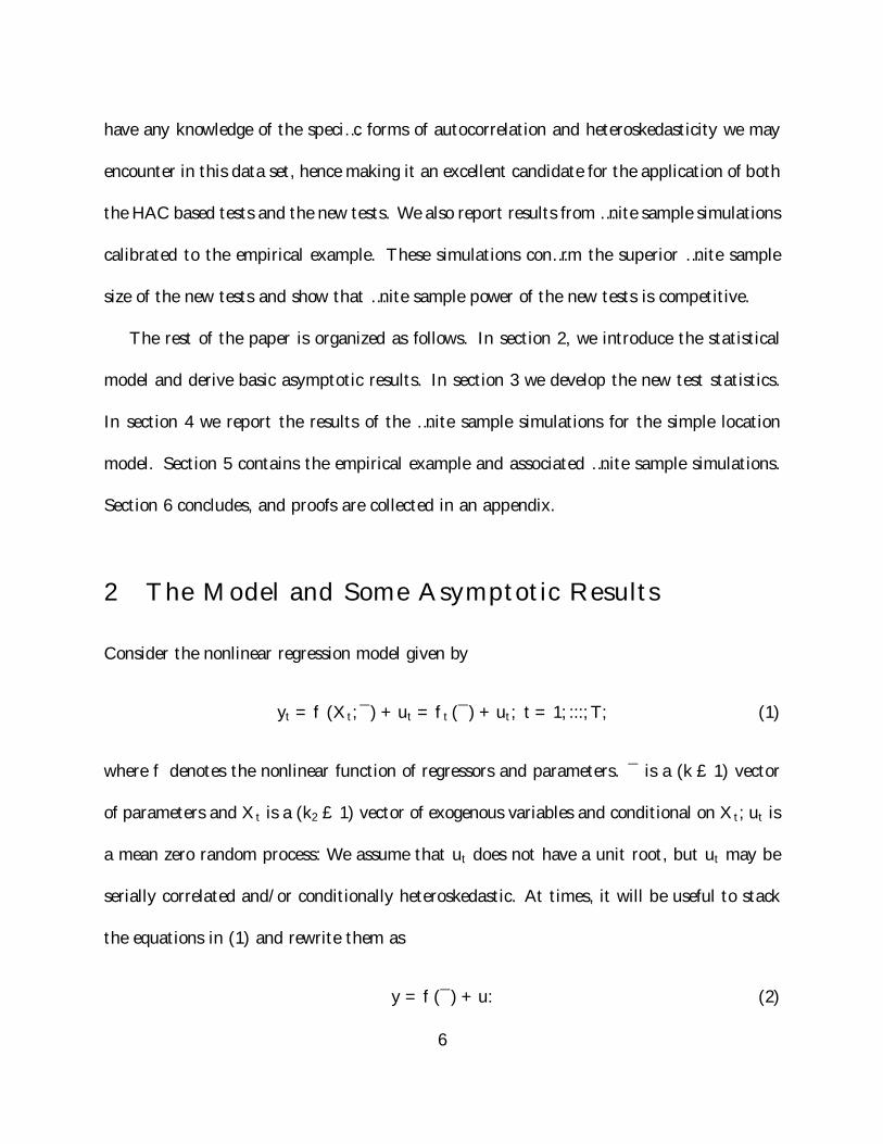
2 The Model and Some Asymptotic Results

Consider the nonlinear regression model given by

yt = f (Xt; ¯) + ut = ft (¯) + ut; t = 1; :::; T; (1)

where f denotes the nonlinear function of regressors and parameters. ¯ is a (k £ 1) vector

of parameters and Xt is a (k2 £ 1) vector of exogenous variables and conditional on Xt; ut is

a mean zero random process: We assume that ut does not have a unit root, but ut may be

serially correlated and/or conditionally heteroskedastic. At times, it will be useful to stack

the equations in (1) and rewrite them as

y = f (¯) + u: (2)

6

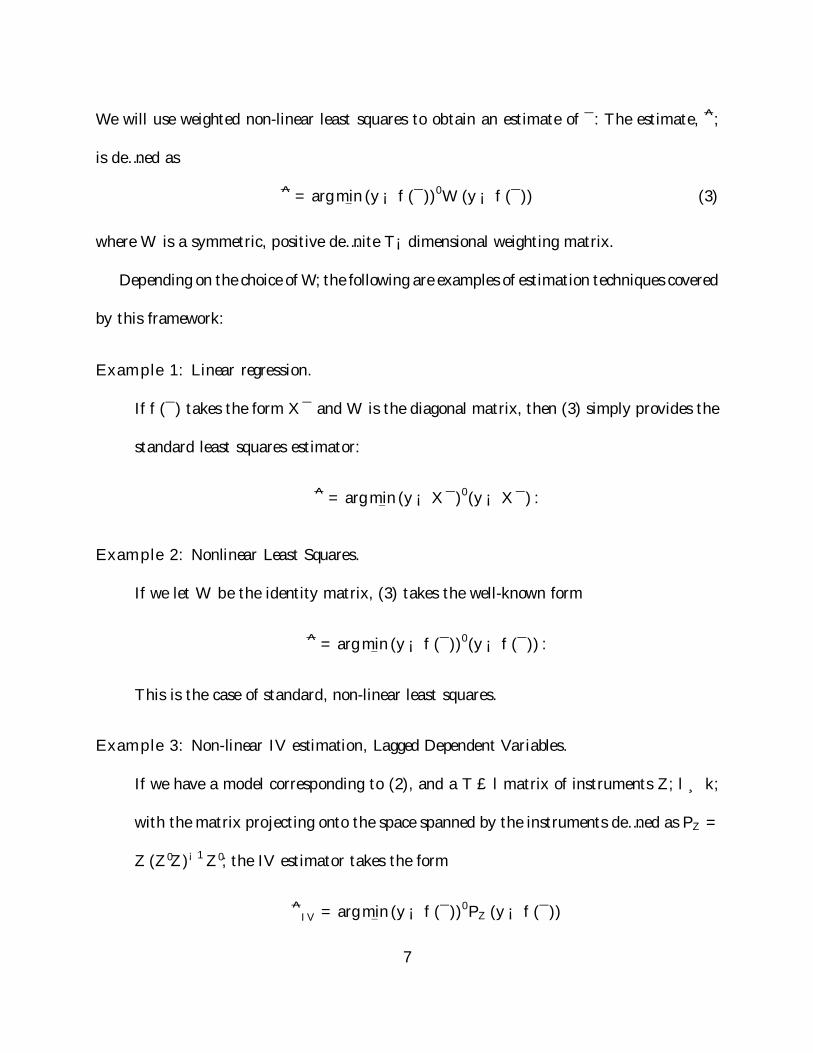
We will use weighted non-linear least squares to obtain an estimate of ¯: The estimate, ^;

is de…ned as

^ = argmin¯

(y ¡ f (¯))0W (y ¡ f (¯)) (3)

where W is a symmetric, positive de…nite T¡dimensional weighting matrix.

Depending on the choice ofW; the following are examples of estimation techniques covered

by this framework:

Example 1: Linear regression.

If f (¯) takes the form X¯ and W is the diagonal matrix, then (3) simply provides the

standard least squares estimator:

^ = argmin¯

(y ¡X¯)0 (y ¡X¯) :

Example 2: Nonlinear Least Squares.

If we let W be the identity matrix, (3) takes the well-known form

^ = argmin¯

(y ¡ f (¯))0 (y ¡ f (¯)) :

This is the case of standard, non-linear least squares.

Example 3: Non-linear IV estimation, Lagged Dependent Variables.

If we have a model corresponding to (2), and a T £ l matrix of instruments Z; l ¸ k;

with the matrix projecting onto the space spanned by the instruments de…ned as PZ =

Z (Z 0Z)¡1 Z 0; the IV estimator takes the form

^IV = argmin

¯(y ¡ f (¯))0 PZ (y ¡ f (¯))

7

corresponding to W = PZ in (3).

A special case is models including lagged dependent variables as regressors. Here we

are interested in a model

y = X¯ + Y2¡ + U; (4)

where Y2 is a matrix containing lagged values of y while ¯ and ¡ are parameters. If we

let A = [X; Y2] and ± = (¯; ¡)0 ; we can rewrite (4) as

y = A± + U:

Using the method of instrumental variables with instruments Z; the estimate of ± is

de…ned as

± = argmin±

(y ¡A±)0 PZ (y ¡A±) (5)

where PZ = Z (Z 0Z)¡1 Z 0: Comparing (5) and (3), we see that ± is the weighted least

squares estimator in a model with weighting matrix PZ.

These examples illustrate that several well-known models and estimation techniques are

special cases of the framework we use.

In developing the tests, we also work with the following transformed model

W12y =W

12 f (¯) +W

12u

or, simplifying the notation

~y = ~f (¯) + ~u (6)

where ~yt; ~ft and ~ut are de…ned in the natural way. The following additional notation is used

throughout the paper. Let the k£1 vector ~Ft (¯) denote the derivative of ~ft (¯) with respect

8

to ¯ and F (¯) the derivative of f (¯) with respect to ¯. In addition, let vt ´ ~Ft (¯) ~ut and

de…ne ­ = ¤¤0 = ¡0 +P1j=1

¡¡j + ¡0j

¢where ¡j = E

¡vtv0t¡j

¢: For later use, note that ­

is equal to 2¼ times the spectral density matrix of vt evaluated at frequency zero. De…ne

St =Ptj=1 vj and let Wk (r) denote a k-vector of independent Wiener precesses, and let

[rT ] denote the integer part of rT; where r 2 [0; 1] : We let ¯0 denote the true value of the

parameter ¯: We use ) to denote weak convergence. The following two assumptions are

su¢cient to obtain the main results of the paper.

Assumption 1 plimhT¡1

P[rT ]t=1

~Ft (¯0) ~F 0t (¯0)i

= rQ 8r 2 [0; 1] ; where Q is invertible.

Furthermore, @@¯0

~Ft (¯0) exists, is uniformly continuous in ¯ for all ¯ in a small open

ball around ¯0 and @@¯0

~Ft (¯0) is bounded in probability.

Assumption 2 T¡ 12S[rT ] = T¡

12P[rT ]t=1

~Ft (¯0) ~ut = T¡12P[rT ]t=1 vt ) ¤Wk (r) :

Assumptions 1 and 2 are more than su¢cient for obtaining an asymptotic normality re-

sult for b: Assumption 1 is fairly standard and rules out trends in the linearized regression

function of the transformed model, but not necessarily in the Xt process. Assumption 1 also

implies the standard assumption that plim£ 1TF

0 (¯0)WF (¯0)¤= Q: On the surface, assump-

tion 2 appears to be stronger than what is necessary compared to the standard approach.

Indeed, to obtain an asymptotic normality result, a conventional central limit theorem for

T¡12PTt=1 vt is all that would be required. However, according to the standard approach,

asymptotically valid testing requires consistent estimation of ­ , i.e. an HAC estimator.

Typical regularity conditions for HAC estimators to be consistent are that the fvtg process

be fourth order stationary and satisfy well known mixing conditions (see Andrews (1991)

9

for details). Interestingly, our assumption 2 holds under the weaker condition that the fvtg

process is only second order (2 + ²; ² > 0) stationary and mixing (see Phillips and Durlauf

(1986) for details). Therefore, we are able to obtain asymptotically valid tests under weaker

regularity conditions than the standard approach.

Using assumptions 1 and 2, we obtain the well known asymptotic normality of ^:

pT

³^ ¡ ¯0

´) Q¡1¤Wk (1) » N

¡0; Q¡1¤¤0Q¡1

¢= N

¡0; Q¡1­Q¡1

¢= N (0; V ) : (7)

The asymptotic distribution is a k-variate normal distribution with mean zero and variance

covariance matrix V = Q¡1­Q¡1: The asymptotic distribution of ^ can be used to test

hypothesis about ¯: In the standard approach an estimate of V (and therefore Q¡1 and ­) is

required: A natural estimate of Q is bQ = 1TF

0³^´WF

³^´: ­ can be estimated by a HAC

estimator, ­: Letting ut be the residuals of the transformed model, the HAC estimate would

utilize vt = ~Ft³^´ut to estimate nonparametrically the spectral density of vt at frequency

zero, and hence ­: A typical estimator takes the form

b­ =T¡1X

j=¡(T¡1)k(j=M)b¡j

with

b¡j = T¡1TX

t=j+1

bvtbv0t¡j for j ¸ 0; b¡j = T¡1TX

t=¡j+1

bvt+jbv0t for j < 0;

where k(x) is a kernel function satisfying k(x) = k(¡x), k(0) = 1, jk(x)j · 1, k(x) contin-

uous at x = 0 andR1¡1 k

2(x)dx < 1. The parameter, M , is often called the truncation

lag. A typical condition for consistency of b­ is that M ! 1 as T ! 1 but M=T ! 0.

For example, the rule M = cT 1=3 where c is any positive constant satis…es this asymptotic

10

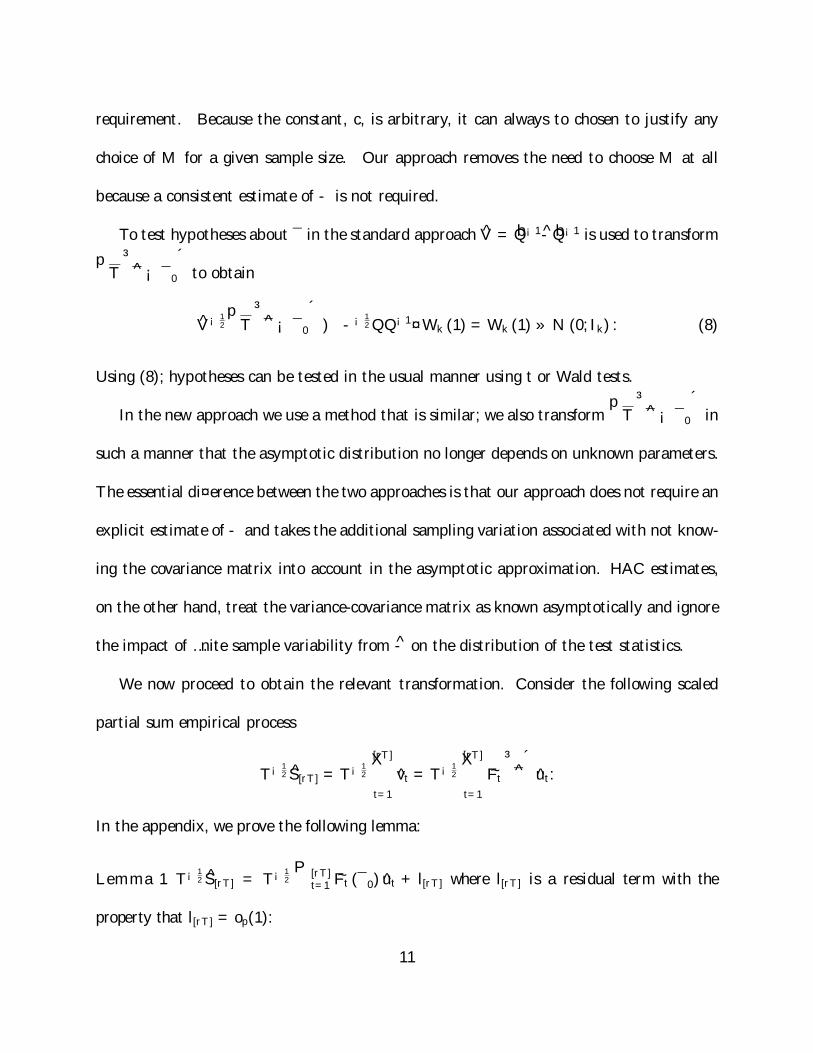
requirement. Because the constant, c, is arbitrary, it can always to chosen to justify any

choice of M for a given sample size. Our approach removes the need to choose M at all

because a consistent estimate of ­ is not required.

To test hypotheses about ¯ in the standard approach V = bQ¡1­ bQ¡1 is used to transformpT

³^ ¡ ¯0

´to obtain

V ¡12pT

³^ ¡ ¯0

´) ­¡

12QQ¡1¤Wk (1) =Wk (1) » N (0; Ik) : (8)

Using (8); hypotheses can be tested in the usual manner using t or Wald tests.

In the new approach we use a method that is similar; we also transformpT

³^ ¡ ¯0

´in

such a manner that the asymptotic distribution no longer depends on unknown parameters.

The essential di¤erence between the two approaches is that our approach does not require an

explicit estimate of ­ and takes the additional sampling variation associated with not know-

ing the covariance matrix into account in the asymptotic approximation. HAC estimates,

on the other hand, treat the variance-covariance matrix as known asymptotically and ignore

the impact of …nite sample variability from ­ on the distribution of the test statistics.

We now proceed to obtain the relevant transformation. Consider the following scaled

partial sum empirical process

T¡12 S[rT ] = T¡

12

[rT ]X

t=1

vt = T¡12

[rT ]X

t=1

~Ft³^´ut:

In the appendix, we prove the following lemma:

Lemma 1 T¡ 12 S[rT ] = T¡

12P[rT ]t=1

~Ft (¯0) ut + l[rT ] where l[rT ] is a residual term with the

property that l[rT ] = op(1):

11

Using this lemma it follows that

T¡12 S[rT ] = T¡

12

[rT ]X

t=1

~Ft (¯0) ut + l[rT ]

= T¡12

[rT ]X

t=1

~Ft (¯0)h~ft (¯0) + ~ut ¡ ~ft

³^´i

+ l[rT ]

= T¡12

[rT ]X

t=1

~Ft (¯0) ~ut + T¡ 1

2

[rT ]X

t=1

~Ft (¯0)h~ft (¯0) ¡ ~ft

³^´i

+ l[rT ]:

Using a Taylor expansion of ~ft(^) around ¯0; we see ~ft(^) = ~ft (¯0)+ ~F 0t³Ä´(^¡¯0); where

Ä 2h^;¯0

i: This expansion allows us to write

T¡12 S[rT ] = T¡

12S[rT ] ¡ T¡

12

[rT ]X

t=1

~Ft (¯0) ~F 0t³Ä´³

^ ¡ ¯0´+ l[rT ] (9)

= T¡12S[rT ] ¡ r

24 1rT

[rT ]X

t=1

~Ft (¯0) ~F 0t³Ä´35pT

³^ ¡ ¯0

´+ op (1) :

Applying assumptions 1 and 2 and equation (7) to (9) gives the asymptotic result

T¡12 S[rT ] ) ¤Wk (r) ¡ rQ

£Q¡1¤Wk (1)

¤= ¤(Wk (r) ¡ rWk (1)) : (10)

Note that (Wk (r) ¡ rWk (1)) is a k-dimensional Brownian Bridge.

Now consider C = T¡2PTt=1 StS

0t: From (10) and the continuous mapping theorem, it

follows that

C = T¡1TX

t=1

³T¡

12 St

´³T¡

12 St

´0) ¤

Z 1

0(Wk (r) ¡ rWk (1)) (Wk (r) ¡ rWk (1))0 dr¤0:

De…ne Pk ´R 10 (Wk (r) ¡ rWk (1)) (Wk (r) ¡ rWk (1))0 dr: The asymptotic distribution of C

can then be written as ¤Pk¤0:We have now obtained a matrix whose asymptotic distribution

is a quadratic form in ¤: In what follows, this enables us to apply a transformation to

12

pT

³^ ¡ ¯0

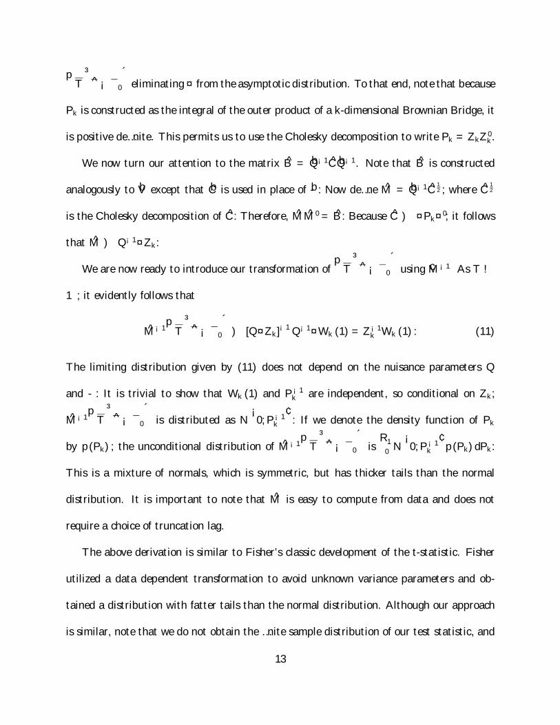
´eliminating ¤ from the asymptotic distribution. To that end, note that because

Pk is constructed as the integral of the outer product of a k-dimensional Brownian Bridge, it

is positive de…nite. This permits us to use the Cholesky decomposition to write Pk = ZkZ 0k.

We now turn our attention to the matrix B = bQ¡1C bQ¡1. Note that B is constructed

analogously to bV except that bC is used in place of b­: Now de…ne M = bQ¡1C 12 ; where C

12

is the Cholesky decomposition of C: Therefore, MM 0 = B: Because C ) ¤Pk¤0; it follows

that M ) Q¡1¤Zk:

We are now ready to introduce our transformation ofpT

³^ ¡ ¯0

´using cM¡1 As T !

1; it evidently follows that

M¡1pT³^ ¡ ¯0

´) [Q¤Zk]

¡1Q¡1¤Wk (1) = Z¡1k Wk (1) : (11)

The limiting distribution given by (11) does not depend on the nuisance parameters Q

and ­: It is trivial to show that Wk (1) and P¡1k are independent, so conditional on Zk;

M¡1pT³^ ¡ ¯0

´is distributed as N

¡0; P¡1k

¢: If we denote the density function of Pk

by p (Pk) ; the unconditional distribution of M¡1pT³^ ¡ ¯0

´is

R 10 N

¡0; P¡1k

¢p (Pk) dPk:

This is a mixture of normals, which is symmetric, but has thicker tails than the normal

distribution. It is important to note that M is easy to compute from data and does not

require a choice of truncation lag.

The above derivation is similar to Fisher’s classic development of the t-statistic. Fisher

utilized a data dependent transformation to avoid unknown variance parameters and ob-

tained a distribution with fatter tails than the normal distribution. Although our approach

is similar, note that we do not obtain the …nite sample distribution of our test statistic, and

13

that Z¡1k Wk (1) is not a multivariate t distribution.

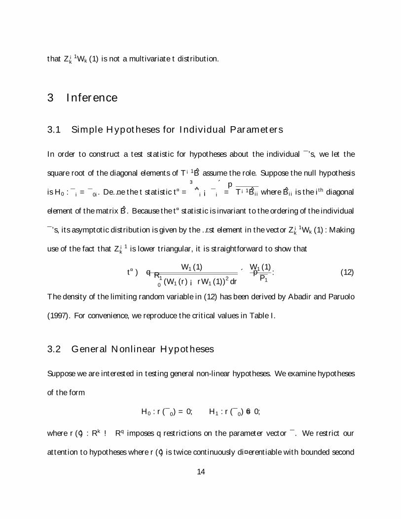
3 Inference

3.1 Simple Hypotheses for Individual Parameters

In order to construct a test statistic for hypotheses about the individual ¯’s, we let the

square root of the diagonal elements of T¡1B assume the role. Suppose the null hypothesis

is H0 : ¯i = ¯0i. De…ne the t statistic t¤ =³^i ¡ ¯i

´=pT¡1Bii where Bii is the ith diagonal

element of the matrix B. Because the t¤ statistic is invariant to the ordering of the individual

¯’s, its asymptotic distribution is given by the …rst element in the vector Z¡1k Wk (1) :Making

use of the fact that Z¡1k is lower triangular, it is straightforward to show that

t¤ ) W1 (1)qR 10 (W1 (r) ¡ rW1 (1))

2 dr´ W1 (1)p

P1: (12)

The density of the limiting random variable in (12) has been derived by Abadir and Paruolo

(1997). For convenience, we reproduce the critical values in Table I.

3.2 General Nonlinear Hypotheses

Suppose we are interested in testing general non-linear hypotheses. We examine hypotheses

of the form

H0 : r (¯0) = 0; H1 : r (¯0) 6= 0;

where r (¢) : Rk ! Rq imposes q restrictions on the parameter vector ¯. We restrict our

attention to hypotheses where r (¢) is twice continuously di¤erentiable with bounded second

14

derivatives near ¯0; andR (¢) ´ @@¯0 r (¢) has full rank q in a neighborhood around ¯0; implying

that there are genuinely q restrictions. For later use, de…ne R = R³^´

and R0 = R (¯0) :

The relevant test statistic is analogous to the standard Wald (or F ) statistic for non-linear

models. We simply substitute B for the standard variance-covariance matrix to obtain

F ¤ = T r³^´0 hRBR0

i¡1r³^´=q:

The asymptotic distribution of F ¤ follows from application of the delta method to r³^´

and

is given by the following theorem which is proved in the appendix.

Theorem 2 Suppose that Assumptions 1 and 2 hold. Then under the null hypothesis H0 :

r (¯0) = 0; F ¤ )Wq (1)0 P¡1q Wq (1) =q as T ! 1:

With F ¤ we have constructed a test for general nonlinear hypotheses of the parameters in a

broad class of non-linear models. The asymptotic distribution depends only on the number

of restrictions (as would a standard Wald test). The density of Wq (1)0 P¡1q Wq (1) =q has

not been derived to our knowledge. However, critical values are easily simulated, and we

tabulate critical values in Table II for q = 1; 2; 3; :::; 30:

4 Finite Sample Evidence in a Simple Location Model

In this section, we consider the …nite sample performance of the t¤ statistic in a simple special

case of our more general framework. Consider a simple location model with AR(1) serially

correlated data:

yt = ¯ + ut; t = 1; ::; T; (13)

15

ut = ½ut¡1 + "t;

"t » iid N (0; 1) :

Inference regarding ¯ even in this simple model can often be related to interesting empirical

applications. For example, Zambrano and Vogelsang (2000) used this simple model to test

the Law of Demand which is one of the core ideas in economics. Another example is testing

whether the radon level in the basement of a house exceeds the limit recommended by the

Environmental Protection Agency. When radon levels are measured in a house, typically

hourly readings are taken over some short time period like 48 hours. This generates time

series data that is highly serially correlated. The relevant question is whether the ”average”

radon level exceeds the cuto¤. In other words, the question is whether an estimate of ¯ in

model (13) is consistent with a true value of ¯ above the cuto¤.

To make matters concrete suppose the null hypothesis of interest is H0 : ¯ · 0 and the

alternative hypothesis is H0 : ¯ > 0: Suppose we estimate ¯ by least squares to obtain b =

T¡1PTt=1 yt:We compare the performance of t¤ to several HAC based t statistics. Note that

all of the t statistics can be written as b=se(b). The …rst statistic, labelled, tHAC, uses a HAC

standard error calculated using the quadratic spectral kernel as recommended by Andrews

(1991). The truncation lag is chosen using the data dependent method recommended

by Andrews (1991) based on an AR(1) plug-in formula (see Andrews (1991) for details).

The second statistic, tPARM uses a standard error calculated using a parametric estimate

of ­ given by e­ = s2"=(1 ¡ b½)2 where b½ =PTt=2 butbut¡1=

PTt=2 bu2t¡1; but = yt ¡ b and s2" =

(T ¡ 1)¡1PTt=2b"2t where b"t = but¡b½but¡1. Note that in practice, the form of serial correlation

16

is usually unknown so that tPARM is not often feasible. It is included here as a benchmark.

Some authors in the HAC literature, most notably Andrews and Monahan (1992), have

recommended using prewhitened spectral density estimators. Therefore, we also implement

t¤ and tHAC using AR(1) prewhitening. The idea is to take b"t and then calculate b­ (or

bC for the case of t¤) and then ”recolor” these estimates by multiplying by (1 ¡ b½)¡2. The

prewhitened statistics are denoted by tHAC¡PW and t¤PW .

We generated data according to (13) under the null hypothesis of ¯ = 0: We computed

empirical null rejection probabilities of the t tests using 5% (right tail) asymptotic critical

values. We report results for ½ = ¡0:5;¡0:3; 0:0; 0:3; 0:5; 0:7; 0:9; 0:95; 0:99 and sample sizes

of T = 25; 50; 100; 200: We used 10,000 replications in all cases. The results are given in

Table III. In nearly all cases, the t¤ statistic has empirical rejection probabilities closest to

the nominal level of 0.05. When prewhitening is used and the sample size is 200, as long as

½ · 0:7, t¤ has empirical rejection probabilities almost exactly equal to 0.05 unlike the other

t tests: When ½ is close to one, all of the statistics are size distorted, but the distortions for

t¤ are always much less.

Why is the asymptotic approximation so much better for t¤ compared to the more stan-

dard t statistics? Consider the standard tests. Asymptotic standard normality of these tests

follows by appealing to consistency of the estimated asymptotic variance. In a sense, merely

appealing to consistency of the estimated asymptotic variance leads to a poor asymptotic

approximation: If one is interested in testing hypotheses about ¯; then an asymptotic nor-

mality result forpT (b ¡ ¯) is required. This is a …rst order asymptotic approximation for

17

the sampling behavior of b. But, this approximation cannot be used itself because there is

an unknown asymptotic variance. Simply replacing the unknown asymptotic variance with

an estimator, i.e. studentizing, and appealing to consistency of that estimator does not fully

preserve the …rst order asymptotic approximation (consistency is a less than …rst order ap-

proximation). In other words, the sampling variability of the variance estimator is ignored

in the asymptotics (the unknown variance is treated as known). Therefore, the …rst order

asymptotic approximation is not ”complete” for the standard tests. On the other hand, the

asymptotic approximation for t¤ captures the sampling variability of the standard error to

…rst order through the random variable,pP1, that appears in the denominator. Thus, the

…rst order asymptotic approximation for t¤ can be viewed as ”complete” and is hence more

accurate in …nite samples. Note that we are not claiming that our asymptotic approxima-

tion for t¤ is more accurate than …rst order (i.e. second order). There may still be room

for further improvements in accuracy that could perhaps be obtained via bootstrapping or

other resampling methods.

5 Empirical Nonlinear Regression: Example and Fur-

ther Finite Sample Evidence

In this section we illustrate the new tests using an empirical example that includes a non-

linear regression model. We wish to examine the e¤ects of growth in U.S. Gross Domestic

Product (GDP) on the growth of aggregate restaurant revenues. Let ¢RR denote the …rst

18

di¤erence of the natural logarithm of real, seasonally adjusted aggregate restaurant revenues

for the United States, and ¢GDP denote the …rst di¤erence of the natural logarithm of real,

seasonally adjusted GDP. Initially, we consider the basic regression model

¢RRt = ¯1 + ¯2¢GDPt + ut; (14)

where ¯1 is an intercept term, while ¯2 is the parameter measuring the long run e¤ect of

GDP growth on restaurant revenues. It is well known that macroeconomic aggregates are

serially correlated over time. To eliminate some of the autocorrelation in the error structure,

we consider an AR(1) transformation of the model. The idea is to ”soak” up some of the

autocorrelation using the AR(1) transformation and then use HAC robust t tests or t¤ to

deal with any remaining autocorrelation in the model. Therefore, consider the model:

¢RRt ¡ ½¢RRt¡1 = ¯1 (1 ¡ ½) + ¯2 (¢GDPt ¡ ½¢GDPt¡1) + ut; t ¸ 2 (15)

¡1 ¡ ½2

¢ 12 ¢RR1 =

¡1 ¡ ½2

¢ 12 ¯1 +

¡1 ¡ ½2

¢ 12 ¯2¢GDP1 + u1

where ¢RRt¡1 and ¢GDPt¡1 are lagged values of …rst di¤erences of real log-restaurant

revenue and real log-GDP respectively. Model (15) is a nonlinear regression that can be

estimated by NLS using a grid search over values of ½.

We use quarterly data from 1971 through 1996 (a total of 104 observations). The restau-

rant revenues are total for all sectors and the source is Current Business Reports, published

by the Bureau of the Census. The real GDP series was obtained from the Survey of Current

Business published by the Bureau of Economic Analysis, US Department of Commerce and

is seasonally adjusted. We converted nominal restaurant revenue to real revenue by dividing

19

by the GDP de‡ator price index also obtained from the Survey of Current Business. We are

interested in ¯2; the long-run e¤ect of GDP growth on the growth of restaurant revenues:

We computed 95% con…dence intervals for ¯2 using t¤ and tHAC. We implemented tHAC as

recommended by Andrews (1991) using the quadratic spectral kernel with a data dependent

truncation lag based on the V AR(1) plug-in method (see Andrews (1991) for details). Table

IV summarizes the results. We see that the di¤erent methods of calculating con…dence

intervals result in di¤erent intervals, and that t¤ provides a tighter con…dence interval than

tHAC .

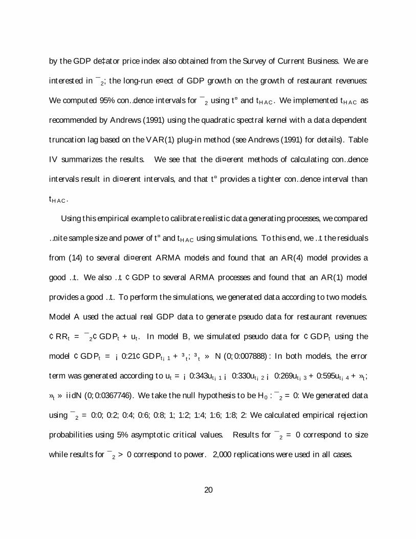
Using this empirical example to calibrate realistic data generating processes, we compared

…nite sample size and power of t¤ and tHAC using simulations. To this end, we …t the residuals

from (14) to several di¤erent ARMA models and found that an AR(4) model provides a

good …t. We also …t ¢GDP to several ARMA processes and found that an AR(1) model

provides a good …t. To perform the simulations, we generated data according to two models.

Model A used the actual real GDP data to generate pseudo data for restaurant revenues:

¢RRt = ¯2¢GDPt + ut. In model B, we simulated pseudo data for ¢GDPt using the

model ¢GDPt = ¡0:21¢GDPt¡1 + ³t; ³t » N (0; 0:007888) : In both models, the error

term was generated according to ut = ¡0:343ut¡1 ¡ 0:330ut¡2 ¡ 0:269ut¡3 + 0:595ut¡4 + »t;

»t » iidN (0; 0:0367746). We take the null hypothesis to be H0 : ¯2 = 0: We generated data

using ¯2 = 0:0; 0:2; 0:4; 0:6; 0:8; 1; 1:2; 1:4; 1:6; 1:8; 2: We calculated empirical rejection

probabilities using 5% asymptotic critical values. Results for ¯2 = 0 correspond to size

while results for ¯2 > 0 correspond to power. 2,000 replications were used in all cases.

20

The results are summarized in Table V. We see that t¤ dominates tHAC with respect to

size. There is signi…cantly less distortion in the sense that the …nite sample size of t¤ is closer

to the nominal level of 5% than for the other statistics. The fact that tHAC is so undersized

explains why the empirical con…dence intervals are wider. No single test dominates in terms

of power and in many cases, t¤ has the highest power.

6 Conclusion

In this paper, we have developed test statistics to test possibly non-linear hypotheses in

nonlinear, weighted regression models with errors that have serial correlation and/or het-

eroskedasticity of unknown form. These tests are simple and do not require use of het-

eroskedasticity autocorrelation consistent (HAC) estimators. Thus, our approach avoids the

pitfalls associated with the choice of truncation lag required when using HAC estimators. We

derived the limiting null distributions of these new tests in a general nonlinear setting, and

showed that while the tests have nonstandard distributions, the distributions depend only

upon the number of restrictions, and critical values were easily obtained using simulations.

Monte Carlo simulations show that in …nite samples the …rst order asymptotic approxima-

tion for the new tests is more accurate than the …rst order asymptotic approximation for

standard tests. The simulations also show that the new tests have competitive power.

21

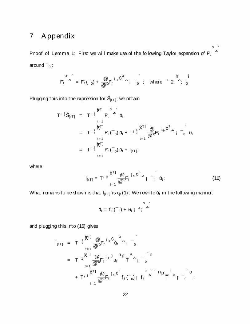
7 Appendix

Proof of Lemma 1: First we will make use of the following Taylor expansion of ~Ft³^´

around ¯0 :

~Ft³^´= ~Ft (¯0) +

@@¯0

~Ft¡¹¢ ³

^ ¡ ¯0´; where ¹ 2

h^; ¯0

i

Plugging this into the expression for S[rT ]; we obtain

T¡12 S[rT ] = T¡

12

[rT ]X

t=1

~Ft³^´ut

= T¡12

[rT ]X

t=1

~Ft (¯0) ut + T¡ 1

2

[rT ]X

t=1

@@¯0

~Ft¡¹¢ ³

^ ¡ ¯0´ut

= T¡12

[rT ]X

t=1

~Ft (¯0) ut + l[rT ];

where

l[rT ] = T¡12

[rT ]X

t=1

@@¯0

~Ft¡¹¢ ³

^ ¡ ¯0´ut: (16)

What remains to be shown is that l[rT ] is op (1) : We rewrite ut in the following manner:

ut = ~ft (¯0) + ~ut ¡ ~ft³^´

and plugging this into (16) gives

l[rT ] = T¡12

[rT ]X

t=1

@@¯0

~Ft¡¹¢ut

³^ ¡ ¯0

´

= T¡1[rT ]X

t=1

@@¯0

~Ft¡¹¢

~utnpT

³^ ¡ ¯0

´o

+ T¡1[rT ]X

t=1

@@¯0

~Ft¡¹¢ ³

~ft (¯0) ¡ ~ft³^´´np

T³^ ¡ ¯0

´o:

22

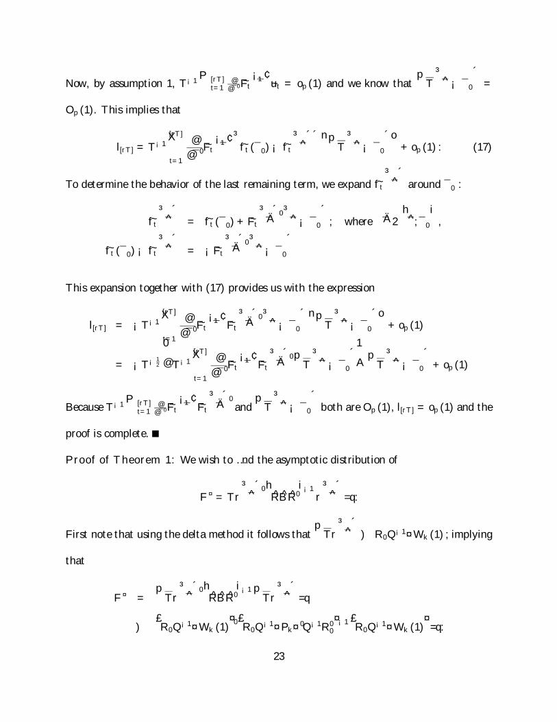
Now, by assumption 1, T¡1P[rT ]t=1

@@¯0

~Ft¡¹¢

~ut = op (1) and we know thatpT

³^ ¡ ¯0

´=

Op (1). This implies that

l[rT ] = T¡1[rT ]X

t=1

@@¯0

~Ft¡¹¢ ³

~ft (¯0) ¡ ~ft³^´´np

T³^ ¡ ¯0

´o+ op (1) : (17)

To determine the behavior of the last remaining term, we expand ~ft³^´

around ¯0 :

~ft³^´

= ~ft (¯0) + ~Ft³Ä´0 ³^ ¡ ¯0

´; where Ä 2

h^; ¯0

i,

~ft (¯0) ¡ ~ft³^´

= ¡ ~Ft³Ä´0 ³^ ¡ ¯0

´

This expansion together with (17) provides us with the expression

l[rT ] = ¡T¡1[rT ]X

t=1

@@¯0

~Ft¡¹¢ ~Ft

³Ä´0 ³^ ¡ ¯0

´npT

³^ ¡ ¯0

´o+ op (1)

= ¡T¡ 12

0@T¡1

[rT ]X

t=1

@@¯0

~Ft¡¹¢ ~Ft

³Ä´0 pT

³^ ¡ ¯0

´1ApT

³^ ¡ ¯0

´+ op (1)

Because T¡1P[rT ]t=1

@@¯0

~Ft¡¹¢ ~Ft

³Ä´0

andpT

³^ ¡ ¯0

´both are Op (1), l[rT ] = op (1) and the

proof is complete.

Proof of Theorem 1: We wish to …nd the asymptotic distribution of

F ¤ = Tr³^´0 hRBR0

i¡1r³^´=q:

First note that using the delta method it follows thatpTr

³^´

) R0Q¡1¤Wk (1) ; implying

that

F ¤ =pTr

³^´0 hRBR0

i¡1 pTr

³^´=q

)£R0Q¡1¤Wk (1)

¤0 £R0Q¡1¤Pk¤0Q¡1R00¤¡1 £R0Q¡1¤Wk (1)

¤=q:

23

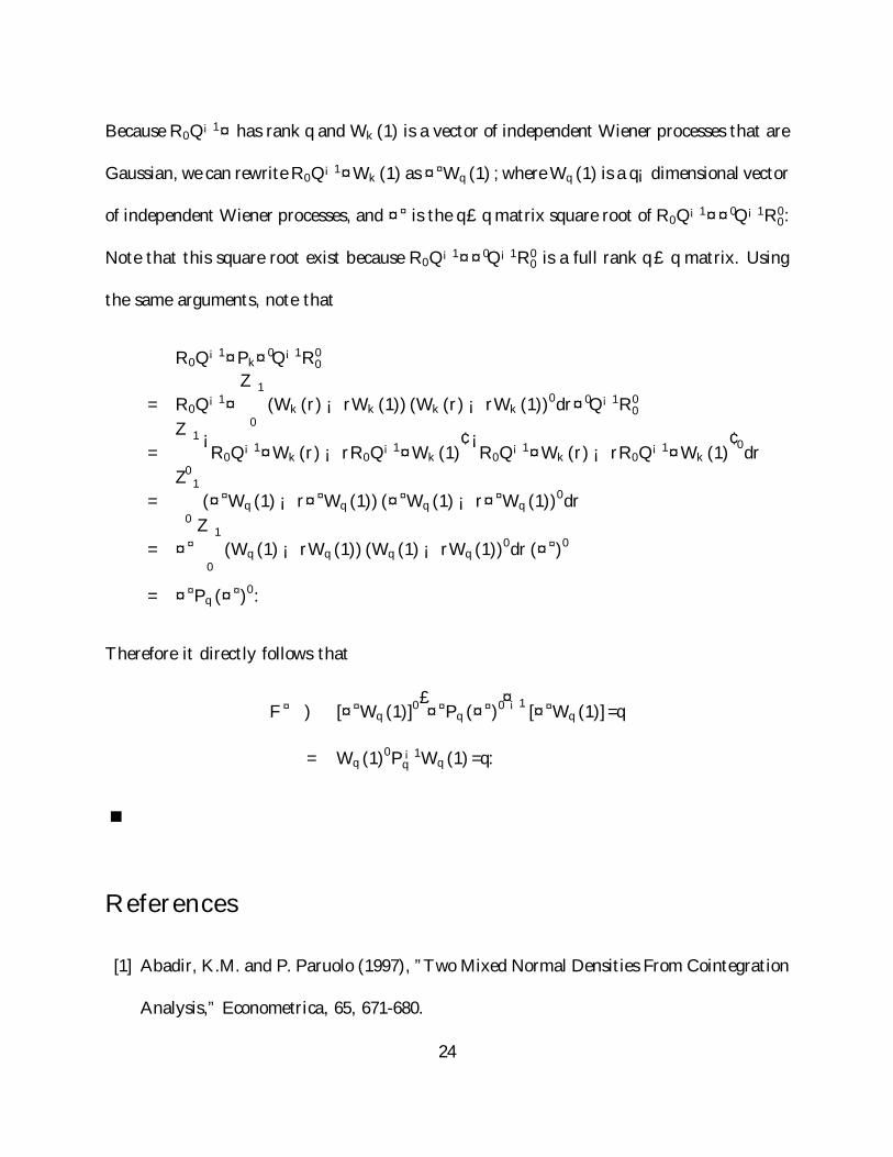
Because R0Q¡1¤ has rank q andWk (1) is a vector of independent Wiener processes that are

Gaussian, we can rewriteR0Q¡1¤Wk (1) as ¤¤Wq (1) ; whereWq (1) is a q¡dimensional vector

of independent Wiener processes, and ¤¤ is the q£q matrix square root of R0Q¡1¤¤0Q¡1R00:

Note that this square root exist because R0Q¡1¤¤0Q¡1R00 is a full rank q£ q matrix. Using

the same arguments, note that

R0Q¡1¤Pk¤0Q¡1R00

= R0Q¡1¤Z 1

0(Wk (r) ¡ rWk (1)) (Wk (r) ¡ rWk (1))0 dr¤0Q¡1R00

=Z 1

0

¡R0Q¡1¤Wk (r) ¡ rR0Q¡1¤Wk (1)

¢ ¡R0Q¡1¤Wk (r) ¡ rR0Q¡1¤Wk (1)

¢0 dr

=Z 1

0(¤¤Wq (1) ¡ r¤¤Wq (1)) (¤¤Wq (1) ¡ r¤¤Wq (1))0 dr

= ¤¤Z 1

0(Wq (1) ¡ rWq (1)) (Wq (1) ¡ rWq (1))0 dr (¤¤)0

= ¤¤Pq (¤¤)0 :

Therefore it directly follows that

F ¤ ) [¤¤Wq (1)]0 £¤¤Pq (¤¤)0

¤¡1 [¤¤Wq (1)] =q

= Wq (1)0 P¡1q Wq (1) =q:

References

[1] Abadir, K.M. and P. Paruolo (1997), ”Two Mixed Normal Densities From Cointegration

Analysis,” Econometrica, 65, 671-680.

24

[2] Andrews, D.W.K. (1991), “Heteroskedasticity and Autocorrelation Consistent Covari-

ance Matrix Estimation,” Econometrica, 59, 817-858.

[3] Andrews, D.W.K. and J.C. Monahan (1992), “An Improved Heteroskedasticity and

Autocorrelation Consistent Covariance Matrix Estimator,” Econometrica, 60, 953-966.

[4] Davidson, R. and J.G. MacKinnon (1993), Estimation and Inference in Econometrics,

New York: Oxford University Press.

[5] Eicker, F. (1967), ”Limit Theorems for Regressions with Unequal and Dependent Er-

rors,” Proceedings of the Fifth Berkeley Symposium on Mathematical Statistics and Prob-

ability, 1, 59-82, Berkeley, University of California Press.

[6] Gallant, A.R. (1987), Nonlinear Statistical Models, New York: Wiley.

[7] Hansen, B.E. (1992), “Consistent Covariance Matrix Estimation for Dependent Het-

erogenous Processes,” Econometrica, 60, 967-972.

[8] Hong, Y. and J. Lee, “Wavelet-based Estimation of Heteroscedasticity and Autocorre-

lation Consistent Covariance Matrices”, Cornell Working paper, October 1999.

[9] Huber, P.J. (1967), ”The Behavior of Maximum Likelihood Estimates Under Nonstan-

dard Conditions,” Proceedings of the Fifth Berkeley Symposium on Mathematical Statis-

tics and Probability, 1, 221-233, Berkeley, University of California Press.

[10] Kiefer, N.M., Vogelsang, T.J, and H. Bunzel (2000), “Simple Robust Testing of Regres-

sion Hypotheses”, Econometrica, 68, 695-714.

25

[11] Newey, W.K. and K.D. West (1987), “A Simple Positive Semi-De…nite, Heteroskedas-

ticity and Autocorrelation Consistent Covariance Matrix,” Econometrica, 55, 703-708.

[12] Phillips, P.C.B. and S.N. Durlauf (1986), “Multiple Time Series Regression with Inte-

grated Processes,” Review of Economic Studies, 53, 473-495.

[13] Priestley, M.B. (1981), Spectral Analysis and Time Series, Vol. 1, Academic Press,

NewYork.

[14] Robinson, P.M (1991), “Automatic Frequency Domain Inference on Semiparametric and

Nonparametric Models”, Econometrica, 59, 1329-1363.

[15] White, H. (1980), ”A Heteroskedasticity-Consistent Covariance Matrix Estimator and

Direct Test for Heterskedasticity,” Econometrica, 48, 817-838.

[16] White, H. (1984), Asymptotic Theory for Econometricians, Orlando: Academic Press.

[17] Zambrano, E. and T.J. Vogelsang (2000), ”A Simple Test of the Law of Demand for the

United States,” Econometrica, 68, 1013-1022.

26

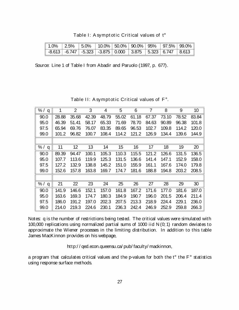
Table I: Asymptotic Critical values of t¤

1.0% 2.5% 5.0% 10.0% 50.0% 90.0% 95% 97.5% 99.0%-8.613 -6.747 -5.323 -3.875 0.000 3.875 5.323 6.747 8.613

Source: Line 1 of Table I from Abadir and Paruolo (1997, p. 677).

Table II: Asymptotic Critical values of F ¤.

% / q 1 2 3 4 5 6 7 8 9 1090.0 28.88 35.68 42.39 48.79 55.02 61.18 67.37 73.10 78.52 83.8495.0 46.39 51.41 58.17 65.33 71.69 78.70 84.63 90.89 96.38 101.897.5 65.94 69.76 76.07 83.35 89.65 96.53 102.7 109.8 114.2 120.099.0 101.2 96.82 100.7 108.4 114.2 121.2 126.9 134.4 139.6 144.9

% / q 11 12 13 14 15 16 17 18 19 2090.0 89.39 94.47 100.1 105.3 110.3 115.5 121.2 126.6 131.5 136.595.0 107.7 113.6 119.9 125.3 131.5 136.6 141.4 147.1 152.9 158.097.5 127.2 132.9 138.8 145.2 151.0 155.9 161.1 167.6 174.0 179.899.0 152.6 157.8 163.8 169.7 174.7 181.6 188.8 194.8 203.2 208.5

% / q 21 22 23 24 25 26 27 28 29 3090.0 141.9 146.6 152.1 157.0 161.8 167.2 171.6 177.0 181.6 187.095.0 163.6 169.3 174.7 180.3 184.9 190.7 196.0 201.5 206.4 211.497.5 186.0 191.2 197.0 202.3 207.5 213.3 218.9 224.4 229.1 236.099.0 214.0 219.3 224.6 230.1 236.3 242.4 246.9 252.9 259.8 266.3

Notes: q is the number of restrictions being tested. The critical values were simulated with100,000 replications using normalized partial sums of 1000 iid N(0; 1) random deviates toapproximate the Wiener processes in the limiting distribution. In addition to this tableJames MacKinnon provides on his webpage,

http://qed.econ.queensu.ca/pub/faculty/mackinnon,

a program that calculates critical values and the p-values for both the t¤ the F ¤ statisticsusing response surface methods.

27

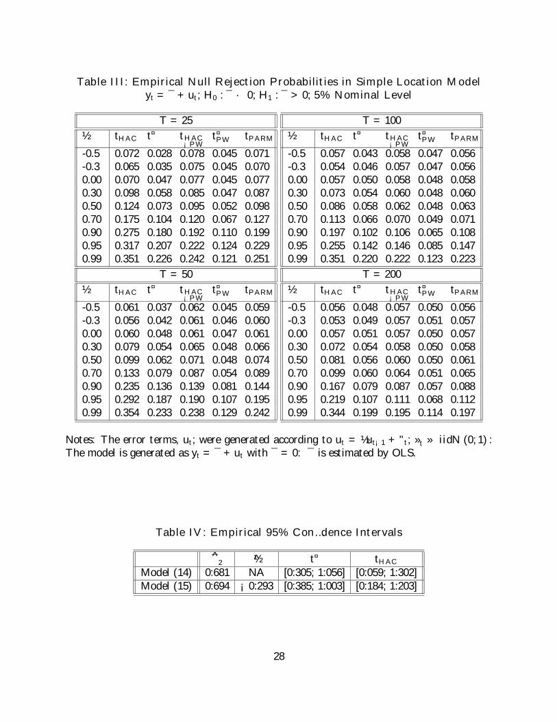
Table III: Empirical Null Rejection Probabilities in Simple Location Modelyt = ¯ + ut; H0 : ¯ · 0; H1 : ¯ > 0; 5% Nominal Level

T = 25½ tHAC t¤ tHAC

¡PWt¤PW tPARM

-0.5 0.072 0.028 0.078 0.045 0.071-0.3 0.065 0.035 0.075 0.045 0.0700.00 0.070 0.047 0.077 0.045 0.0770.30 0.098 0.058 0.085 0.047 0.0870.50 0.124 0.073 0.095 0.052 0.0980.70 0.175 0.104 0.120 0.067 0.1270.90 0.275 0.180 0.192 0.110 0.1990.95 0.317 0.207 0.222 0.124 0.2290.99 0.351 0.226 0.242 0.121 0.251

T = 50½ tHAC t¤ tHAC

¡PWt¤PW tPARM

-0.5 0.061 0.037 0.062 0.045 0.059-0.3 0.056 0.042 0.061 0.046 0.0600.00 0.060 0.048 0.061 0.047 0.0610.30 0.079 0.054 0.065 0.048 0.0660.50 0.099 0.062 0.071 0.048 0.0740.70 0.133 0.079 0.087 0.054 0.0890.90 0.235 0.136 0.139 0.081 0.1440.95 0.292 0.187 0.190 0.107 0.1950.99 0.354 0.233 0.238 0.129 0.242

T = 100½ tHAC t¤ tHAC

¡PWt¤PW tPARM

-0.5 0.057 0.043 0.058 0.047 0.056-0.3 0.054 0.046 0.057 0.047 0.0560.00 0.057 0.050 0.058 0.048 0.0580.30 0.073 0.054 0.060 0.048 0.0600.50 0.086 0.058 0.062 0.048 0.0630.70 0.113 0.066 0.070 0.049 0.0710.90 0.197 0.102 0.106 0.065 0.1080.95 0.255 0.142 0.146 0.085 0.1470.99 0.351 0.220 0.222 0.123 0.223

T = 200½ tHAC t¤ tHAC

¡PWt¤PW tPARM

-0.5 0.056 0.048 0.057 0.050 0.056-0.3 0.053 0.049 0.057 0.051 0.0570.00 0.057 0.051 0.057 0.050 0.0570.30 0.072 0.054 0.058 0.050 0.0580.50 0.081 0.056 0.060 0.050 0.0610.70 0.099 0.060 0.064 0.051 0.0650.90 0.167 0.079 0.087 0.057 0.0880.95 0.219 0.107 0.111 0.068 0.1120.99 0.344 0.199 0.195 0.114 0.197

Notes: The error terms, ut; were generated according to ut = ½ut¡1 + "t; »t » iidN (0; 1) :The model is generated as yt = ¯ + ut with ¯ = 0: ¯ is estimated by OLS.

Table IV: Empirical 95% Con…dence Intervals

^2 ½ t¤ tHAC

Model (14) 0:681 NA [0:305; 1:056] [0:059; 1:302]Model (15) 0:694 ¡0:293 [0:385; 1:003] [0:184; 1:203]

28

Table V: Empirical Rejection Probabilities, Model (14)T = 103, 5% Nominal Level.

Power is Size Adjusted Power not Size AdjustedDGP ¯0 t¤ tHAC t¤ tHAC

A 0.0 0.028 0.006 0.028 0.0060.2 0.158 0.177 0.101 0.0390.4 0.429 0.504 0.339 0.1870.6 0.744 0.813 0.652 0.4730.8 0.925 0.961 0.871 0.7501.0 0.978 0.993 0.957 0.9111.2 0.994 1.000 0.988 0.9791.4 1.000 1.000 0.996 0.9951.6 1.000 1.000 1.000 1.0001.8 1.000 1.000 1.000 1.0002.0 1.000 1.000 1.000 1.000

B 0.0 0.046 0.031 0.046 0.0310.2 0.108 0.106 0.098 0.0700.4 0.252 0.289 0.233 0.2230.6 0.449 0.542 0.423 0.4590.8 0.628 0.739 0.607 0.6781.0 0.768 0.872 0.753 0.8331.2 0.867 0.941 0.854 0.9161.4 0.924 0.976 0.913 0.9631.6 0.954 0.990 0.947 0.9851.8 0.972 0.997 0.967 0.9952.0 0.980 0.998 0.977 0.997

Notes: For both models, pseudo data for ¢RRt was generated using (14) with the error termsgiven by ut = ¡0:343ut¡1 ¡ 0:330ut¡2 ¡ 0:269ut¡3 + 0:595ut¡4 + »t; »t » N (0; 0:0367746) :Model A uses the original ¢GDPt data as the regressor, while Model B generates the GDPseries according to the following process: ¢GDPt = ¡0:21¢¢GDPt+³t; ³t » N (0; 0:007888) :The slanted script provide empirical null rejection probabilites while the other table entriesare …nite sample power.

29