Optimization Methods and Software

Vol. 00, No. 00, Month 200x, 1–20

Classification model selection via bilevel programming

G. KUNAPULI*†, K. P. BENNETT†, JING HU† and JONG-SHI PANG‡

†Department of Mathematical Sciences,

Rensselaer Polytechnic Institute, 110 8th Street, Troy NY 12180.

‡ Department of Industrial and Enterprise Systems Engineering,

University of Illinois at Urbana-Champaign, 104 S. Mathews Ave., Urbana IL 61801.

(Received 31 July 2006; revised 24 January 2007; in final form 23 October 2007)

Support vector machines and related classification models require the solution of convex optimizationproblems that have one or more regularization hyper-parameters. Typically, the hyper-parametersare selected to minimize cross validated estimates of the out-of-sample classification error of themodel. This cross-validation optimization problem can be formulated as a bilevel program inwhich the outer-level objective minimizes the average number of misclassified points across thecross-validation folds, subject to inner-level constraints such that the classification functions for eachfold are (exactly or nearly) optimal for the selected hyper-parameters. Feature selection is includedin the bilevel program in the form of bound constraints in the weights. The resulting bilevel problemis converted to a mathematical program with linear equilibrium constraints, which is solved usingstate-of-the-art optimization methods. This approach is significantly more versatile than commonlyused grid search procedures, enabling, in particular, the use of models with many hyper-parameters.Numerical results demonstrate the practicality of this approach for model selection in machinelearning.

Keywords: Support vector classification; Cross validation; Bilevel Programming; Model Selection;Feature Selection

1 Introduction

Support Vector Machines (SVM) [1,2] are one of the most widely used methodsfor classification. The underlying quadratic programming problem is convex(thus, is generally not difficult to deal with, both theoretically and compu-tationally), but typically it contains hyper-parameters that must be selectedby the users. Despite many interesting attempts to use bounds or other tech-niques [3–5], the most widely accepted and commonly used method for select-

∗Corresponding author. Email: kunapg@rpi.edu

2 Kunapuli, Bennett, Hu, and Pang

ing these hyper-parameters is still based on minimizing cross-validated esti-mates of the classification errors. For example, one might define a grid overthe hyper-parameters of interest, and then perform 10-fold cross validation foreach of the grid values. Since the size of the grid grows exponentially with thenumber of hyper-parameters, grid search becomes prohibitively expensive fora large number of parameters. In this work, we use bilevel programming toidentify hyper-parameters for classification problems.

The work nontrivially extends our recent work on applying the methodologyof bilevel programming to parameter identification problems in machine learn-ing. The motivation and benefits of the bilevel approach are explained in ourprevious paper, [6], where we have discussed the application to constrainedregression within the framework of cross validation. In essence, unlike manytraditional grid search methods used in machine learning that are severelyrestricted by the number of hyper-parameters to be searched, the bilevel ap-proach enables the identification of many such parameters all at once by wayof the state-of-the-art optimization methods and their softwares (such as thosepublicly available on the neos servers). Another important advantage of thebilevel approach is its modeling versatility in handling multiple machine learn-ing goals simultaneously and efficiently; these include optimal choice of modelparameters [3, 7], feature selection for dimension reduction [8], inexact crossvalidation, kernelization to handle nonlinear data sets [9], and variance controlfor fold consistency through multi-tasking.

Solution path methods [5, 10] also tackle selection of regularization param-eters as a continuous optimization problem using parametric linear/quadraticprogramming, which necessarily restricts the selection to one single parameteronly. These methods solve the problem of picking the best parameter using onetraining set and one testing set very efficiently. One paper used this approachto optimize parameters [11] by combining the solution paths of the two pathsfor each of the two parameters. Solution path approaches are a special caseof the bilevel approach, but the bilevel approach is far more general in that itcan be applied to many parameters and alternative measures of generalization,based on many solutions such as cross-validation.

From the optimization point of view, bilevel programs resulting from theseapplications belong to the general class of mathematical programs with equi-librium constraints (MPECs), [12], for which there are extensive advances intheory, algorithms, and software in recent years. Some selected references fo-cusing on algorithm developments and analysis include [13–25].

We focus on the bilevel binary classification problem where the main taskis to classify data into two groups according to a linear model using a clas-sical support-vector (SV) classifier [1]. The hyper-parameters are selected tominimize the T -fold cross validated estimate of the out-of-sample misclassi-fication error. Each fold of training defines an inner-level convex quadratic

Bilevel Model Selection for Classification 3

program (QP) with parameters constrained by some bounds that are part ofthe overall variables to be optimized; such bounds provide a mechanism forfeature selection whereby those features corresponding to small bounds in thesolution of the bilevel problem will be deemed insignificant. The outer-levelproblem minimizes the T -fold average classification error based on the optimalsolutions of the inner-level QPs for all possible hyper-parameters. Using theapproach in [26], we add inner-level linear programs to compute the numberof misclassified test points for each fold. In principle, the objective functionsin the inner-level classification optimization problems could be rather general;the only restriction we impose is their convexity so that the only non-convexitygenerated by the inner-level problems in the MPEC is essentially the comple-mentarity slackness in the optimality conditions of the inner-level problems.

The organization of the paper is as follows. In Section 2, we present themathematical formulation of the bilevel cross validation classification modeland show how it can be converted to an instance of an MPEC. In Section 3,we illustrate the power of the formulations to address variations of the classi-fication problems. In Section 4, we describe grid search and present a relaxednonlinear programming reformulation of the MPEC called inexact cross vali-dation. In Section 5, we describe the experimental setup, the data sets used,and present some computational results comparing the grid search and bilevelcross validation methods. We conclude the paper with some final remarks inSection 6.

2 Model Formulation

We first say a few words about our notation. Let Ω denote a given finite setof ℓ = |Ω| labeled data points, (xi, yi)ℓ

i=1 ⊂ Rn+1. Since we are interested in

the binary classification case, the labels yi are ±1. Let the set of indices forthe points in Ω be N = 1, . . . , ℓ. For T -fold cross validation, Ω is partitionedinto T pairwise disjoint subsets, Ωt, called the validation sets. The sets Ωt =Ω \Ωt are the training sets within each fold. The corresponding index sets forthe validation and training sets are Nt and N t respectively. The hyperplanetrained within the t-th fold using the training set Ωt is identified by the pair(wt, bt) ∈ R

n+1. For compactness of notation, the vectors wt are collected,column-wise, into the matrix W ∈ R

n×T , and the scalars bt into the vectorb ∈ R

T . A vector of ones of arbitrary dimension is denoted by 1. Given twovectors, r and s ∈ R

n, the complementarity condition r ⊥ s means r ′s = 0,where the prime ′ denotes the transpose; and r⋆ denotes the step functionapplied to each component of the vector r as defined in (7).

The well-known SV classification problem depends on a nonnegative regu-larization parameter, λ, which is selected through cross validation based on

4 Kunapuli, Bennett, Hu, and Pang

the average misclassification error measured on the out-of-sample data, i.e, thevalidation sets. Specifically, the basic bilevel model for support vector classifi-cation, is formulated as follows:

minimizeW,b,λ,w

Θ(W,b)

subject to λ lb ≤ λ ≤ λ ub, w lb ≤ w ≤ w ub ,

and for t = 1, . . . , T,

(1)

(wt, bt) ∈ arg min−w≤w≤w

b∈R

λ

2‖w ‖2

2 +∑

j∈N t

max(1 − yj(x

′jw − b), 0

)

. (2)

Problem 1 is called the outer-level problem and subproblems 2 are called theinner-level problems. The outer-level objective, Θ(W,b), is some measure ofvalidation accuracy over all the folds, typically the average number of misclas-sifications. There are T inner-level subproblems, one for each fold in T -foldcross validation. The arg min is the last constraint in (1) and denotes the setof all optimal solutions to the T convex optimization problems (2). Each t-thsubproblem is simply a classical support vector classification problem appliedto the corresponding training set, Ωt, along with the additional box constraintof the form −w ≤ w ≤ w, where w is a variable in the overall bilevel opti-mization; in turn, w is restricted to given bounds wub ≥ wlb ≥ 0.

The symmetric box constraint is included for the purposes of wrapper-typefeature selection and regularization. In addition, the box constraint was se-lected to illustrate that the bilevel approach can successfully optimize manyhyper-parameters. Note that there is one box constraint parameter for everydescriptor. Consider a particular feature that is expected to be redundant orirrelevant i.e., that feature does not contribute much to the final classifier.Then, the corresponding weight in w would be small or zero, which, in turn,constrains the corresponding weights in each wt, thereby effectively control-ling their capacity and potentially increasing generalization performance. Thebilevel program will effectively be a wrapper feature selection method. Wrap-per methods search for subsets of feature that optimize estimates of the testinggeneralization error for models trained with those features [27]. Sparse 1-normregularization can also be used for feature selection but the subset features ineach of the CV folds illustrates great variability [8]. The box constraints willensure that a consistent subset of the features will be used across all the folds.If w can be picked effectively, the box constrained SVM, (2), could represent afundamentally new way to perform feature selection. Thus, the box constraintsare embedded in the bilevel cross validation scheme and w becomes a vectorof hyper-parameters in the problem.

Note that we use λ2‖w‖2

2 for regularization rather than the typical term

Bilevel Model Selection for Classification 5

C∑

j∈N t

max(1 − yj(x′jw − b), 0), where C is the parameter to be chosen.

This is due to our empirical observation that the former is more numericallyrobust than the latter within the bilevel setting. Clearly, the two modes ofregularization are equivalent for each inner-level problem with C = 1

λ, provided

that both parameters are positive. Note that the bilevel program selects thehyperparameters. The final classifier can be constructed by optimizing a singleinstance of the lower-level problem using the optimal hyper-parameters andall of the training data. In this case, the final λ should be scaled by T

T−1 toaccount for the larger training set size.

Similar to w, the parameter λ is subject to given bounds λub ≥ λlb > 0. Thisis done for three reasons: first, to facilitate direct comparison with grid searchbased cross validation (see Section 4.2); second, to improve the stability andspeed up convergence of a general purpose NLP solver; and third, to ensurethe positivity of the parameters λ and w: so that the bilevel approach yields,in case of the former, a nonzero regularization parameter, in case of the latter,a nontrivial box constraint for feature selection.

2.1 The inner-level problems

As mentioned above, there are T inner-level problems that model the trainingof classifiers within each fold. Consider the inner-level problem correspondingto the t-th fold i.e., the t-th training set, Ωt, indexed by N t, is used. With λand w fixed in this subproblem, we introduce slack variables, ξt, in (2) to refor-mulate the max function using standard linear programming techniques. Thisgives the the box-constrained SV classifier (BoxSVC) which is nearly identicalto the classical SVM for classification, except that it has the additional boxconstraint for regularization and feature selection:

minimizewt, bt, ξ

t

λ

2‖wt‖2

2 +∑

j∈N t

ξtj

subject to −w ≤ wt ≤ w,

yj(x′jw

t − bt) ≥ 1 − ξtj

ξtj ≥ 0

∀ j ∈ N t.

(3)

The BoxSVC is a convex quadratic program in the variables wt, bt andξt

jj∈N t

. Let γt,− and γt,+ be the multipliers of the lower and upper bound

constraints −w ≤ wt ≤ w respectively and αtj be the multiplier for the hyper-

plane constraint, yj(x′jw

t − bt) ≥ 1− ξtj. Using these multipliers, we can write

down the primal and dual feasibility and complementarity slackness conditions

6 Kunapuli, Bennett, Hu, and Pang

of (3) compactly as follows:

0 ≤ αtj ⊥ yj(x

′jw

t − bt) − 1 + ξtj ≥ 0

0 ≤ ξtj ⊥ 1 − αt

j ≥ 0

∀ j ∈ N t,

0 ≤ γt,+ ⊥ w − wt ≥ 0,

0 ≤ γt,− ⊥ w + wt ≥ 0,

(4)

which together with the following first-order conditions,

λwt −∑

j∈N t

yjαtjxj + γt,+ − γt,− = 0,

∑

j∈N t

yjαtj = 0,

(5)

constitute the Karush-Kuhn-Tucker (KKT) optimality conditions to (3). TheKKT conditions are necessary and sufficient conditions for the optimal solutionof (3). Thus the inner-level optimization problems (2) can be replaced withthe system of equations (4) and (5).

2.2 The outer-level optimization

The inner-level problems solve T box-constrained SV classification problemson the training sets to yield T hyperplanes, (wt, bt), one for each fold. Theouter-level objective function is a measure of generalization error based on theT out-of-sample validation sets, which we minimize. The measure used hereis the classical cross-validation error for classification, the average number ofpoints misclassified. The outer-level objective that achieves this can be writtenusing the step function, ()⋆, as

Θ(W,b) =1

T

T∑

t=1

1

|Nt |∑

i∈Nt

[−yi(x

′iw

t − bt)]⋆. (6)

Note that in the inner summation, Ωt, the t-th validation set, indexed by Nt,is used. The inner summation averages the number of misclassifications withineach fold while the outer summation averages the averaged misclassificationerror over the folds. The step function used in (6) can be defined, componen-

Bilevel Model Selection for Classification 7

twise, for a vector, r, as

(r⋆)i =

1, if ri > 0,0, if ri ≤ 0.

(7)

It is clear that ()⋆ is discontinuous and that (6) cannot be used directly inthe bilevel setting. The step function, however, can be characterized as thesolution to a linear program as demonstrated in [26], i.e.,

r⋆ = arg minζ

−ζ ′r : 0 ≤ ζ ≤ 1. (8)

Thus, we have to solve T linear programs of the form (9) to determine whichvalidation points, xi ∈ Nt, are misclassified within the t-th fold, i.e., whenthe sign of yi(x

′iw

t − bt) is negative. These LPs are inserted as inner-levelproblems into the bilevel setting in order to recast the discontinuous outer-level objective into a continuous one. They yield ζt =

[−yi(x

′iw

t − bt)]⋆, with

ζti = 1 if the point xi is misclassified and 0 otherwise. Finally, it should be

noted that if xi lies on the hyperplane, (wt, bt), then we will have 0 < ζti < 1.

ζt ∈ arg min0≤ζ≤1

∑

i∈Nt

ζiyi

(x ′

iwt − bt

)

. (9)

Returning to the general case, we introduce additional multipliers, z, for theconstraint ζ ≤ 1. Consequently, any solution to (8) should satisfy the followinglinear complementarity conditions:

0 ≤ ζ ⊥−r + z ≥ 0,

0 ≤ z ⊥ 1 − ζ ≥ 0.(10)

We noted in Section 2.1 that the inner-level problems, (2), can be replacedwith the first-order KKT conditions, (4–5). Furthermore, the inner-level stepfunction LPs, (9), can be rewritten using the linear complementarity condi-

8 Kunapuli, Bennett, Hu, and Pang

tions, (10). The overall two-level classification problem becomes

min1

T

T∑

t=1

1

|Nt |∑

i∈Nt

ζti

s. t. λ lb ≤ λ ≤ λ ub, w lb ≤ w ≤ w ub ,

and for t = 1 . . . T,

0 ≤ ζti ⊥ yi

(x ′

iwt − bt

)+ zt

i ≥ 0

0 ≤ zti ⊥ 1 − ζt

i ≥ 0

∀ i ∈ Nt,

0 ≤ αtj ⊥ yj(x

′jw

t − bt) − 1 + ξtj ≥ 0

0 ≤ ξtj ⊥ 1 − αt

j ≥ 0

∀ j ∈ N t,

0 ≤ γt,+ ⊥ w − wt ≥ 0,

0 ≤ γt,− ⊥ w + wt ≥ 0,

λwt −∑

j∈N t

yjαtjxj + γt,+ − γt,− = 0,

∑

j∈N t

yjαtj = 0,

(11)

which is an instance of an MPEC. It is a nonconvex optimization problembecause of the complementarity constraints. We refer to this problem as theBilevel Misclassification Minimization (BilevelMM) problem.

3 Bilevel Classification Variations

There are many possible variations of the bilevel classification problem. Toillustrate the versatility of the bilevel approach, we discuss the outer-levelobjective, feature selection strategies, and kernel selection.

3.1 Outer-level objective

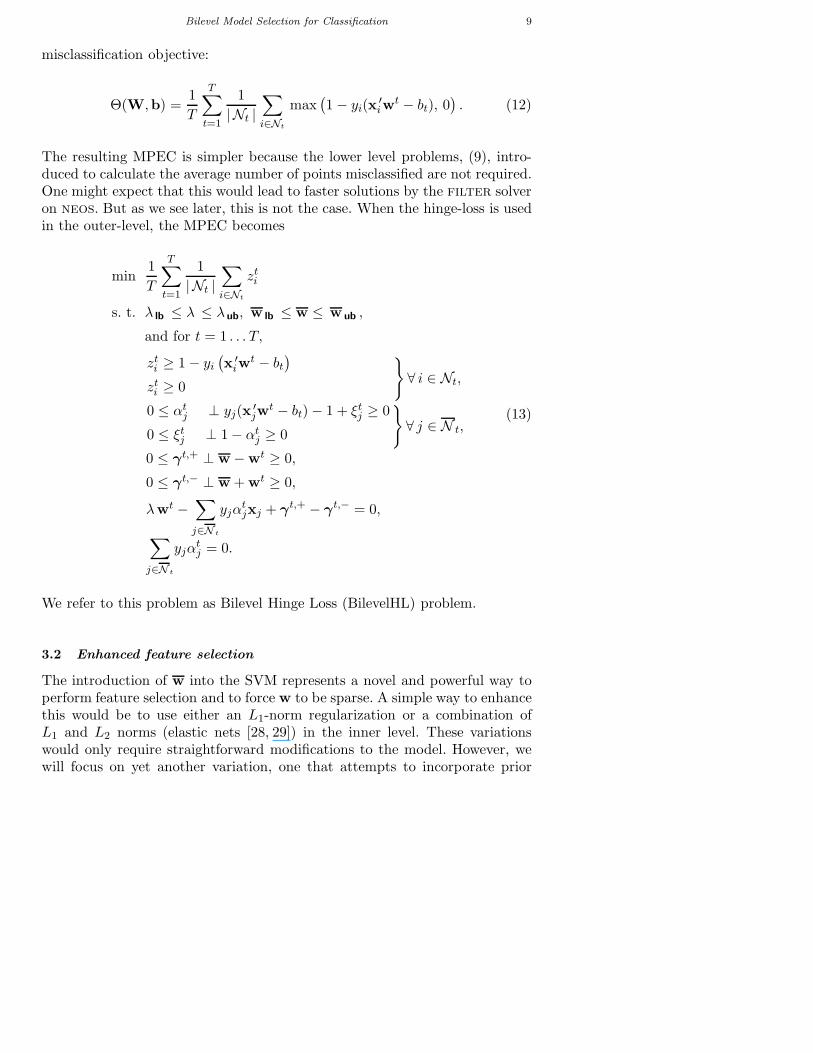
The outer-level objective, (6), is not the only criterion that can be used toestimate generalization error within the cross validation scheme. An intuitivelyappealing alternative is to use the same misclassification measure for both theouter- and inner-level problems. Thus, we can also use the hinge loss, whichminimizes the distance of each misclassified validation point from the classifiermargin trained within each fold. The hinge loss is an upper bound on the

Bilevel Model Selection for Classification 9

misclassification objective:

Θ(W,b) =1

T

T∑

t=1

1

|Nt |∑

i∈Nt

max(1 − yi(x

′iw

t − bt), 0). (12)

The resulting MPEC is simpler because the lower level problems, (9), intro-duced to calculate the average number of points misclassified are not required.One might expect that this would lead to faster solutions by the filter solveron neos. But as we see later, this is not the case. When the hinge-loss is usedin the outer-level, the MPEC becomes

min1

T

T∑

t=1

1

|Nt |∑

i∈Nt

zti

s. t. λ lb ≤ λ ≤ λ ub, w lb ≤ w ≤ w ub ,

and for t = 1 . . . T,

zti ≥ 1 − yi

(x ′

iwt − bt

)

zti ≥ 0

∀ i ∈ Nt,

0 ≤ αtj ⊥ yj(x

′jw

t − bt) − 1 + ξtj ≥ 0

0 ≤ ξtj ⊥ 1 − αt

j ≥ 0

∀ j ∈ N t,

0 ≤ γt,+ ⊥ w − wt ≥ 0,

0 ≤ γt,− ⊥ w + wt ≥ 0,

λwt −∑

j∈N t

yjαtjxj + γt,+ − γt,− = 0,

∑

j∈N t

yjαtj = 0.

(13)

We refer to this problem as Bilevel Hinge Loss (BilevelHL) problem.

3.2 Enhanced feature selection

The introduction of w into the SVM represents a novel and powerful way toperform feature selection and to force w to be sparse. A simple way to enhancethis would be to use either an L1-norm regularization or a combination ofL1 and L2 norms (elastic nets [28, 29]) in the inner level. These variationswould only require straightforward modifications to the model. However, wewill focus on yet another variation, one that attempts to incorporate prior

10 Kunapuli, Bennett, Hu, and Pang

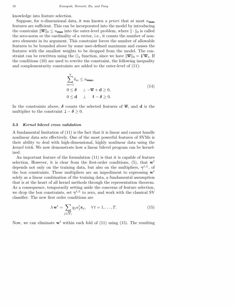
knowledge into feature selection.Suppose, for n-dimensional data, it was known a priori that at most nmax

features are sufficient. This can be incorporated into the model by introducingthe constraint ‖w‖0 ≤ nmax into the outer-level problem, where ‖ · ‖0 is calledthe zero-norm or the cardinality of a vector, i.e., it counts the number of non-zero elements in its argument. This constraint forces the number of allowablefeatures to be bounded above by some user-defined maximum and causes thefeatures with the smallest weights to be dropped from the model. The con-straint can be rewritten using the ()⋆ function, since we have ‖w‖0 = 1′w⋆. Ifthe conditions (10) are used to rewrite the constraint, the following inequalityand complementarity constraints are added to the outer-level of (11):

n∑

m=1

δm ≤ nmax,

0 ≤ δ ⊥ −w + d ≥ 0,

0 ≤ d ⊥ 1− δ ≥ 0.

(14)

In the constraints above, δ counts the selected features of w, and d is themultiplier to the constraint 1− δ ≥ 0.

3.3 Kernel bilevel cross validation

A fundamental limitation of (11) is the fact that it is linear and cannot handlenonlinear data sets effectively. One of the most powerful features of SVMs istheir ability to deal with high-dimensional, highly nonlinear data using thekernel trick. We now demonstrate how a linear bilevel program can be kernel-ized.

An important feature of the formulation (11) is that it is capable of featureselection. However, it is clear from the first-order conditions, (5), that wt

depends not only on the training data, but also on the multipliers, γt,±, ofthe box constraints. These multipliers are an impediment to expressing wt

solely as a linear combination of the training data, a fundamental assumptionthat is at the heart of all kernel methods through the representation theorem.As a consequence, temporarily setting aside the concerns of feature selection,we drop the box constraints, set γt,± to zero, and work with the classical SVclassifier. The new first order conditions are

λwt =∑

j∈N t

yjαtjxj , ∀ t = 1, . . . , T. (15)

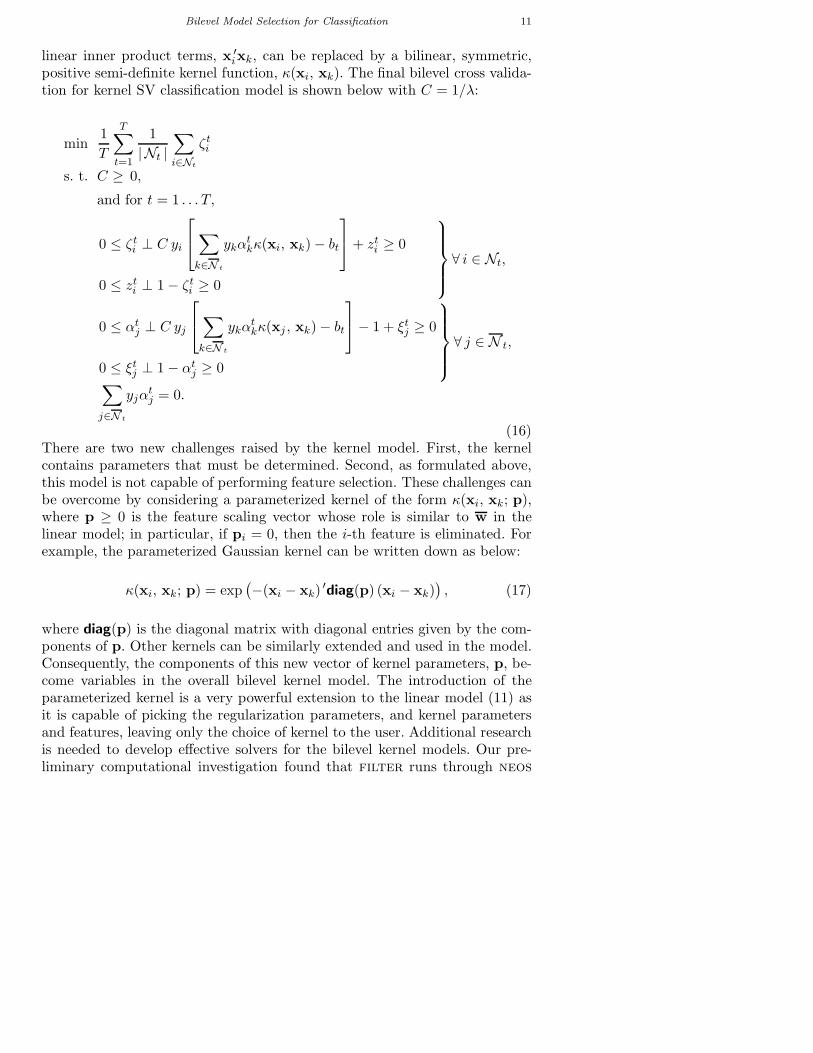
Now, we can eliminate wt within each fold of (11) using (15). The resulting

Bilevel Model Selection for Classification 11

linear inner product terms, x ′ixk, can be replaced by a bilinear, symmetric,

positive semi-definite kernel function, κ(xi, xk). The final bilevel cross valida-tion for kernel SV classification model is shown below with C = 1/λ:

min1

T

T∑

t=1

1

|Nt |∑

i∈Nt

ζti

s. t. C ≥ 0,

and for t = 1 . . . T,

0 ≤ ζti ⊥ C yi

∑

k∈N t

ykαtkκ(xi, xk) − bt

+ zti ≥ 0

0 ≤ zti ⊥ 1 − ζt

i ≥ 0

∀ i ∈ Nt,

0 ≤ αtj ⊥ C yj

∑

k∈N t

ykαtkκ(xj , xk) − bt

− 1 + ξtj ≥ 0

0 ≤ ξtj ⊥ 1 − αt

j ≥ 0

∀ j ∈ N t,

∑

j∈N t

yjαtj = 0.

(16)There are two new challenges raised by the kernel model. First, the kernelcontains parameters that must be determined. Second, as formulated above,this model is not capable of performing feature selection. These challenges canbe overcome by considering a parameterized kernel of the form κ(xi, xk; p),where p ≥ 0 is the feature scaling vector whose role is similar to w in thelinear model; in particular, if pi = 0, then the i-th feature is eliminated. Forexample, the parameterized Gaussian kernel can be written down as below:

κ(xi, xk; p) = exp(−(xi − xk)

′diag(p) (xi − xk)), (17)

where diag(p) is the diagonal matrix with diagonal entries given by the com-ponents of p. Other kernels can be similarly extended and used in the model.Consequently, the components of this new vector of kernel parameters, p, be-come variables in the overall bilevel kernel model. The introduction of theparameterized kernel is a very powerful extension to the linear model (11) asit is capable of picking the regularization parameters, and kernel parametersand features, leaving only the choice of kernel to the user. Additional researchis needed to develop effective solvers for the bilevel kernel models. Our pre-liminary computational investigation found that filter runs through neos

12 Kunapuli, Bennett, Hu, and Pang

could only successfully solve small problems. Thus, the results and discussionin this paper are limited to the linear case.

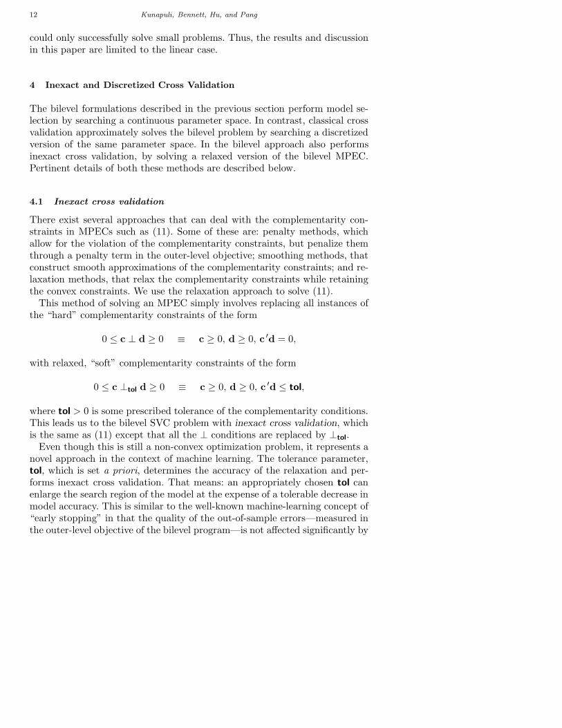
4 Inexact and Discretized Cross Validation

The bilevel formulations described in the previous section perform model se-lection by searching a continuous parameter space. In contrast, classical crossvalidation approximately solves the bilevel problem by searching a discretizedversion of the same parameter space. In the bilevel approach also performsinexact cross validation, by solving a relaxed version of the bilevel MPEC.Pertinent details of both these methods are described below.

4.1 Inexact cross validation

There exist several approaches that can deal with the complementarity con-straints in MPECs such as (11). Some of these are: penalty methods, whichallow for the violation of the complementarity constraints, but penalize themthrough a penalty term in the outer-level objective; smoothing methods, thatconstruct smooth approximations of the complementarity constraints; and re-laxation methods, that relax the complementarity constraints while retainingthe convex constraints. We use the relaxation approach to solve (11).

This method of solving an MPEC simply involves replacing all instances ofthe “hard” complementarity constraints of the form

0 ≤ c ⊥ d ≥ 0 ≡ c ≥ 0, d ≥ 0, c ′d = 0,

with relaxed, “soft” complementarity constraints of the form

0 ≤ c ⊥tol d ≥ 0 ≡ c ≥ 0, d ≥ 0, c ′d ≤ tol,

where tol > 0 is some prescribed tolerance of the complementarity conditions.This leads us to the bilevel SVC problem with inexact cross validation, whichis the same as (11) except that all the ⊥ conditions are replaced by ⊥tol.

Even though this is still a non-convex optimization problem, it represents anovel approach in the context of machine learning. The tolerance parameter,tol, which is set a priori, determines the accuracy of the relaxation and per-forms inexact cross validation. That means: an appropriately chosen tol canenlarge the search region of the model at the expense of a tolerable decrease inmodel accuracy. This is similar to the well-known machine-learning concept of“early stopping” in that the quality of the out-of-sample errors—measured inthe outer-level objective of the bilevel program—is not affected significantly by

Bilevel Model Selection for Classification 13

small perturbations to a computed solution, in turn facilitating an early ter-mination of cross validation. This approach also has the advantage of easingthe difficulty of dealing with the disjunctive nature of the complementarityconstraints. The exact same approach can also be applied to the hinge-lossMPEC, (13).

4.2 Grid search

Classical cross validation is performed by discretizing the parameter space intoa grid and searching for the combination of parameters that minimizes the out-of-sample error, also referred to as validation error. This corresponds to theouter-level objective of the bilevel program (11). Typically, coarse logarithmicparameter grids of base 2 or 10 are used. Once a locally optimal grid point withthe smallest validation error has been found, it may be refined or fine-tunedby a local search.

In the case of SV classification, the only hyper-parameter is the regular-ization constant, λ. However, the bilevel model (11) uses the box-constrainedSVM for feature selection; Grid Search has to determine w as well. It is thissearch in the w-space that causes a serious combinatorial difficulty for thegrid approach. To see this, consider the case of T -fold cross validation usinggrid search, where λ and w are each allowed to take on d discrete values.Assuming the data is n-dimensional, grid search would have to solve roughlyO(Tdn+1) problems. The resulting combinatorial explosion makes grid searchintractable for all but the smallest n. In this paper, to counter this difficulty,we implement the following heuristic scheme:

• To determine λ: Perform a one-dimensional grid search using the classi-cal SVC problem (without the box constraint). The range [λlb, λub] is dis-cretized into a coarse, base-10, logarithmic grid. These grid points constitutethe search space for this step, which we will call unconstrained grid search.At each grid point, T SVC problems are solved on the training sets and theerror is measure on the validation sets. The grid point with the smallestaverage validation error, λ, is “optimal”.

• To determine w: Perform a n-dimensional grid search to determine the rele-vant features of w using the box-constrained SVC problem (BoxSVC) and λobtained from the previous step. Only two distinct choices for each featureare considered: 0, to test feature redundancy, and some large value thatwould not affect the choice of an appropriate feature weight. In this set-ting, 3-fold cross validation would involve solving about O(3 ∗ 2n) BoxSVCproblems. We call this step constrained grid search.

• The number of problems in constrained grid search is already impracticalnecessitating a further restriction of the relevant features to a maximum of

14 Kunapuli, Bennett, Hu, and Pang

Table 1. Descriptions of data sets used.

Data set ℓtrain ℓtest n T

Pima Indians Diabetes Database 240 528 8 3Wisconsin Breast Cancer Database 240 442 9 3Cleveland Heart Disease Database 216 81 14 3Johns Hopkins University Ionosphere Database 240 111 33 3Star/Galaxy Bright Database 600 1862 14 3Star/Galaxy Dim Database 900 3292 14 3

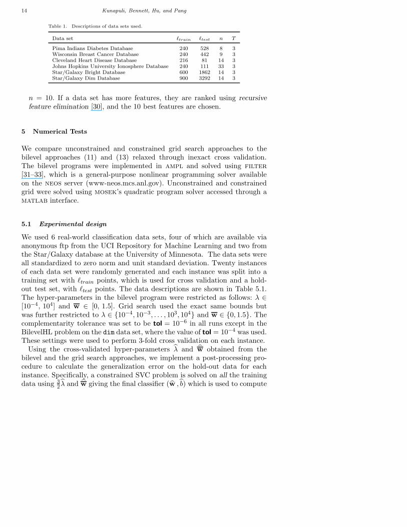
n = 10. If a data set has more features, they are ranked using recursive

feature elimination [30], and the 10 best features are chosen.

5 Numerical Tests

We compare unconstrained and constrained grid search approaches to thebilevel approaches (11) and (13) relaxed through inexact cross validation.The bilevel programs were implemented in ampl and solved using filter

[31–33], which is a general-purpose nonlinear programming solver availableon the neos server (www-neos.mcs.anl.gov). Unconstrained and constrainedgrid were solved using mosek’s quadratic program solver accessed through amatlab interface.

5.1 Experimental design

We used 6 real-world classification data sets, four of which are available viaanonymous ftp from the UCI Repository for Machine Learning and two fromthe Star/Galaxy database at the University of Minnesota. The data sets wereall standardized to zero norm and unit standard deviation. Twenty instancesof each data set were randomly generated and each instance was split into atraining set with ℓtrain points, which is used for cross validation and a hold-out test set, with ℓtest points. The data descriptions are shown in Table 5.1.The hyper-parameters in the bilevel program were restricted as follows: λ ∈[10−4, 104] and w ∈ [0, 1.5]. Grid search used the exact same bounds butwas further restricted to λ ∈ 10−4, 10−3, . . . , 103, 104 and w ∈ 0, 1.5. Thecomplementarity tolerance was set to be tol = 10−6 in all runs except in theBilevelHL problem on the dim data set, where the value of tol = 10−4 was used.These settings were used to perform 3-fold cross validation on each instance.

Using the cross-validated hyper-parameters λ and w obtained from thebilevel and the grid search approaches, we implement a post-processing pro-cedure to calculate the generalization error on the hold-out data for eachinstance. Specifically, a constrained SVC problem is solved on all the trainingdata using 3

2 λ and w giving the final classifier (w , b) which is used to compute

Bilevel Model Selection for Classification 15

1 2 3 4 5 6 7 8 9 10 110.18

0.19

0.2

0.21

0.22

0.23

0.24

0.25

0.26

0.27

0.28

Number of folds

Ave

rage

Err

or r

ate

(%)

Hold−out Test ErrorCross validation Error

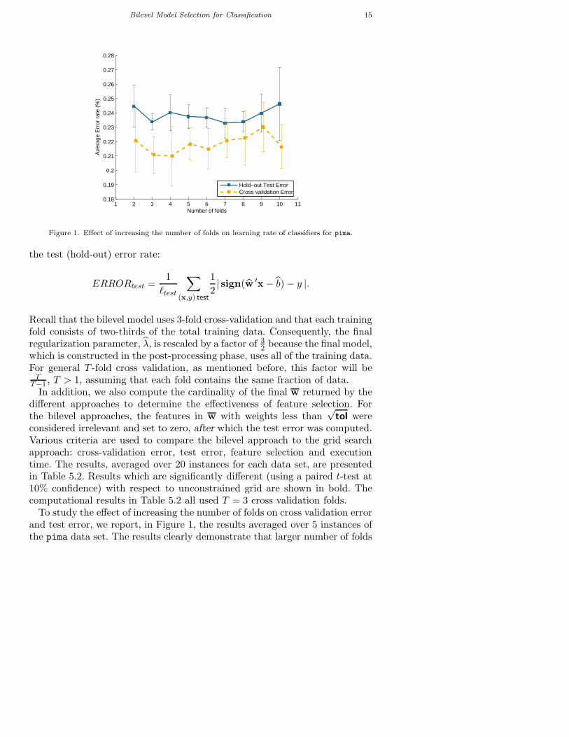
Figure 1. Effect of increasing the number of folds on learning rate of classifiers for pima.

the test (hold-out) error rate:

ERRORtest =1

ℓtest

∑

(x,y) test

1

2| sign(w ′x− b) − y |.

Recall that the bilevel model uses 3-fold cross-validation and that each trainingfold consists of two-thirds of the total training data. Consequently, the finalregularization parameter, λ, is rescaled by a factor of 3

2 because the final model,which is constructed in the post-processing phase, uses all of the training data.For general T -fold cross validation, as mentioned before, this factor will be

TT−1 , T > 1, assuming that each fold contains the same fraction of data.

In addition, we also compute the cardinality of the final w returned by thedifferent approaches to determine the effectiveness of feature selection. Forthe bilevel approaches, the features in w with weights less than

√tol were

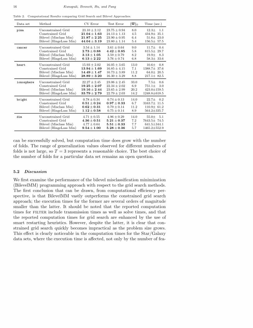
considered irrelevant and set to zero, after which the test error was computed.Various criteria are used to compare the bilevel approach to the grid searchapproach: cross-validation error, test error, feature selection and executiontime. The results, averaged over 20 instances for each data set, are presentedin Table 5.2. Results which are significantly different (using a paired t-test at10% confidence) with respect to unconstrained grid are shown in bold. Thecomputational results in Table 5.2 all used T = 3 cross validation folds.

To study the effect of increasing the number of folds on cross validation errorand test error, we report, in Figure 1, the results averaged over 5 instances ofthe pima data set. The results clearly demonstrate that larger number of folds

16 Kunapuli, Bennett, Hu, and Pang

Table 2. Computational Results comparing Grid Search and Bilevel Approaches.

Data set Method CV Error Test Error ‖w‖0 Time (sec.)

pima Unconstrained Grid 23.10 ± 2.12 23.75 ± 0.94 8.0 12.3± 1.1Constrained Grid 21.04± 1.63 24.13 ± 1.13 4.5 434.9± 35.1Bilevel (Misclass Min) 21.87± 2.25 23.90 ± 0.95 6.4 51.8± 23.0Bilevel (HingeLoss Min) 44.04± 3.19 23.80 ± 1.14 5.4 156.5± 57.5

cancer Unconstrained Grid 3.54 ± 1.14 3.61 ± 0.64 9.0 11.7± 0.4Constrained Grid 2.73 ± 0.88 4.42 ± 0.85 5.8 815.5± 29.7Bilevel (Misclass Min) 3.13 ± 1.05 3.59 ± 0.79 8.2 19.9± 8.3Bilevel (HingeLoss Min) 6.13 ± 2.22 3.76 ± 0.74 6.8 58.3± 33.6

heart Unconstrained Grid 15.93 ± 2.02 16.05 ± 3.65 13.0 10.6± 0.8Constrained Grid 13.94± 1.69 16.85 ± 4.15 7.1 1388.7± 37.6Bilevel (Misclass Min) 14.49± 1.47 16.73 ± 3.89 11.2 64.0± 20.5Bilevel (HingeLoss Min) 28.89± 3.20 16.30 ± 3.29 8.8 217.1± 82.5

ionosphere Unconstrained Grid 22.27 ± 2.45 23.06 ± 2.45 33.0 7.5± 0.6Constrained Grid 19.25± 2.07 22.34 ± 2.02 6.9 751.1± 3.0Bilevel (Misclass Min) 19.16± 2.44 23.65 ± 2.99 20.2 423.0±159.5Bilevel (HingeLoss Min) 33.79± 2.79 22.79 ± 2.03 14.2 1248.8±618.5

bright Unconstrained Grid 0.78 ± 0.34 0.74 ± 0.13 14.0 22.7± 0.2Constrained Grid 0.51 ± 0.24 0.97 ± 0.33 6.7 3163.7± 11.5Bilevel (Misclass Min) 0.62 ± 0.31 0.79 ± 0.14 11.2 110.9± 61.2Bilevel (HingeLoss Min) 1.12 ± 0.58 0.75 ± 0.14 8.9 564.2±335.7

dim Unconstrained Grid 4.71 ± 0.55 4.96 ± 0.29 14.0 55.0± 5.1Constrained Grid 4.36 ± 0.51 5.21 ± 0.37 7.2 7643.5± 74.5Bilevel (Misclass Min) 4.77 ± 0.64 5.51 ± 0.33 7.7 641.5±344.1Bilevel (HingeLoss Min) 9.54 ± 1.00 5.28 ± 0.36 5.7 1465.2±552.9

can be successfully solved, but computation time does grow with the numberof folds. The range of generalization values observed for different numbers offolds is not large, so T = 3 represents a reasonable choice. The best choice ofthe number of folds for a particular data set remains an open question.

5.2 Discussion

We first examine the performance of the bilevel misclassification minimization(BilevelMM) programming approach with respect to the grid search methods.The first conclusion that can be drawn, from computational efficiency per-spective, is that BilevelMM vastly outperforms the constrained grid searchapproach; the execution times for the former are several orders of magnitudesmaller than the latter. It should be noted that the reported computationtimes for filter include transmission times as well as solve times, and thatthe reported computation times for grid search are enhanced by the use ofsmart restarting heuristics. However, despite the latter, it is clear that con-strained grid search quickly becomes impractical as the problem size grows.This effect is clearly noticeable in the computation times for the Star/Galaxydata sets, where the execution time is affected, not only by the number of fea-

Bilevel Model Selection for Classification 17

tures, but also by the data set sizes, which contain hundreds of training points.BilevelMM, on the other hand, is capable of cross-validating the dim data set,with 900 training points, in around 10-11 minutes on average. This suggeststhat the scalability of the bilevel approach could be improved significantly byexploiting the structure and sparsity inherent in SVMs. Research is currentlyunderway in this direction and findings will be reported elsewhere.

With regard to generalization error, two interesting points emerge. First,the BilevelMM approach consistently produces results that are comparableto, if not slightly better than the grid search approaches, in spite of the factthat the cross-validation error is typically higher. This can be attributed to thefact that general-purpose NLP solvers tend to converge to acceptable solutions,with no guarantee of global optimality. Second, the only exception is the dim

data set where the slight degradation in generalization performance can beimputed to numerical difficulties experienced by the NLP solvers because oflarge dimensionality and large data set size. Again, a specialized algorithmthat could guarantee global optimality could produce better generalizationperformance.

With regard to feature selection, it is clear that unconstrained grid performsnone at all, while, interestingly, constrained grid search uses less features thanBilevelMM, albeit at the expense of excessive computational times and poorergeneralization. This can be attributed to the fact that constrained grid isgreedy, i.e., it analyzes every combination of features to find an optimal setand performs feature selection aggressively on data sets with more than 10features as it drops the remaining features using RFE. BilevelMM has nosuch heuristic or mechanism to drive the number of selected features down.Despite this, it is clear that it does succeed in performing a better trade-offbetween feature selection and generalization. See Section 3.2 for ideas thatmight improve feature selection in the bilevel setting.

Next, we discuss the performance of the bilevel hinge-loss (BilevelHL) ap-proach and compare it to BilevelMM. The most striking difference is in thecomputation times of the two approaches, with BilevelHL, quite unexpectedly,taking two to three times longer. We theorize that this is because BilevelMMhas many more stationary points (for an intuitive explanation of this curiousproperty that is endemic to misclassification minimization problems, see [26])than BilevelHL and consequently, a general-purpose NLP solver tends to con-verge to stationarity faster. However, BilevelHL is still considerably faster thangrid search; again, the only exception being the ionosphere data set. It shouldbe noted that constrained grid search used only 10 features—after recursivefeature elimination was used to drop 23 of the 33 features—while BilevelHLsolved the full problem using all the features. If constrained grid were to useall 33 features, it would have to solve around O(1011) BoxSVC problems.

In terms of generalization error, BilevelHL performs as well or better than

18 Kunapuli, Bennett, Hu, and Pang

BilevelMM and never significantly worse than unconstrained grid (except forthe dim data set), despite the fact that the CV errors of BilevelHL are uni-formly higher. Recall that a complementarity tolerance of 10−4 was used forthe dim data set. This was to relax the problem further for the numerical sta-bility of the NLP solver. This relaxation, however, leads to a slight degradationin the quality of the solution.

Finally, BilevelHL tends to pick fewer features than BilevelMM, butstill more than constrained grid. This comparison between BilevelMM andBilevelHL indicates that the best choice of outer-level objective is still anopen question in need of further research.

6 Conclusions

We demonstrated how T -fold cross-validation can be cast as a continuousbilevel program: inner-level problems are introduced for each of the T -folds tocompute classifiers on the training sets and to calculate the misclassificationerrors on the training sets within each fold. Furthermore, we introduced thebox-constrained SVM which has a hyper-parameter for each feature to per-form feature selection. The resulting bilevel program is converted to an MPEC,which is in turn converted to a nonlinear programming problem through in-exact cross validation. The advantage of the bilevel approach is that manyhyper-parameters can be optimized simultaneously, unlike prior grid searchapproaches that are practically limited to one or two parameters. Initial com-putational results using filter through neos were very promising. High qual-ity solutions were found using few features using much less computation timethan grid search approaches over the same hyper-parameters.

This work represents a first proof of concept. We showed that cross-validation through minimization of different objectives such as averaged mis-classification error and hinge loss could be solved efficiently with large numbersof hyper-parameters. The resulting classifiers demonstrated good generaliza-tion ability and were dependent on only a few features. The success of thesetwo different bilevel approaches suggests that other changes in the objectiveand regularization can lead to further enhancement of performance for classifi-cation problems. Furthermore, the versatility of the bilevel approach suggeststhat further variations could be developed to tackle other challenges in machinelearning such as missing data, semi-supervised learning, kernel learning andmulti-task learning. Future theoretical and computational work is needed toinvestigate this flexibility–that the bilevel approach has the ability to optimizelarge number of hyper-parameters for many types of outer-level objectives.

A major outstanding research question is the development of efficient opti-mization algorithms for the bilevel program. Our current work is limited to

Bilevel Model Selection for Classification 19

the use of an off-the-shelf NLP solver. A recent linear time SVM algorithm cansolve traditional SVM classification problems with millions of data points [34]using advanced decomposition techniques that exploit the underlying structureof the problem. Many other efficient and scalable methods for SVM aboundand these methods should be compared with and incorporated into the bilevelapproach [35, 36]. Solution path algorithms traverse the feasible regions forvery limited bilevel problems. The hope is that by developing related specialpurpose solvers the scalability of the bilevel program can be achieved as well.

Acknowledgement

This work was supported in part by the Office of Naval Research under grantno. N00014-06-1-0014.

References

[1] Cortes, C. and Vapnik, V., 1995, Support-vector networks. Machine Learning, 20, 273–297.[2] Vapnik, V., 2000, The Nature of Statistical Learning Theory (2nd edn) (New York, NY: Springer-

Verlag).[3] Chapelle, O, Vapnik, V., Bousquet, O. and Mukherjee, S., 2002, Choosing multiple parameters

for support vector machines. Machine Learning, 46, 131–159.[4] Duan, K., Keerthi, S. and Poo, A., 2003, Evaluation of simple performance measures for tuning

SVM hyperparameters. Neurocomputing, 51, 41–59.[5] Hastie, T., Rossett, S., Tibshirani, R. and Zhu, J., 2004, The entire regularization path for the

support vector machine. Journal of Machine Learning Research, 5, 1391-1415.[6] Bennett, K. P., Ji, X., Hu, J., Kunapuli, G. and Pang, J.-S., 2006, Model selection via bilevel

programming. Proceedings of the IEEE International Joint Conference on Neural Networks,Vancouver, B.C., Canada, July 16–21, 1922–1929.

[7] Golub, G., Heath, M. and Wahba, G., 1979, Generalised cross validation as a method for choosinga good ridge parameter. Technometrics, 21, 215–223.

[8] Bi, J., Bennett, K. P., Embrechts, M., Breneman, C. and Song, M., 2003, Dimensionality reduc-tion via sparse support vector machines. Journal on Machine Learning Research, 3, 1229–1243.

[9] Shawe-Taylor, J. and Cristianini, N., 2004, Kernel Methods for Pattern Analysis (Cambridge,UK: Cambridge University Press).

[10] Zhu, J., Rosset, S., Hastie, T. and Tibshirani, R., 2003, 1-norm support vector machines. Ad-vances in Neural Information Processing Systems, 16.

[11] Wang, G., Yeung, D. and Lochovsky, F., 2006, Two-dimensional solution path for support vectorregression. Proceedings of the 23th International Conference on Machine Learning, 148, 993–1000.

[12] Luo, Z. Q., Pang, J.-S. and Ralph, D., 1996, Mathematical Programs With Equilibrium Con-straints (Cambridge, UK: Cambridge University Press).

[13] Anitescu, M., 2005, On solving mathematical programs with complementarity constraints asnonlinear programs. SIAM Journal on Optimization, 15, 1203–1236.

[14] Anitescu, M., Tseng, P. and Wright, S. J., 2005, Elastic-mode algorithms for mathematical pro-grams with equilibrium constraints: Global convergence and stationarity properties. PreprintANL/MCS-P1242-0405, Mathematics and Computer Science Division, Argonne National Lab-oratory.

[15] Dempe, S., 2002, Foundations of Bilevel Programming. (Dordrecht, The Netherlands: KluwerAcademic Publishers).

[16] Dempe, S., 2003, Annotated bibliography on bilevel programming and mathematical programswith equilibrium constraints. Optimization, 52, 333–359.

20 Kunapuli, Bennett, Hu, and Pang

[17] Fletcher, R. and Leyffer, S., 2004, Solving mathematical programs with complementarity con-straints as nonlinear programs. Optimization Methods and Software, 19, 15-40.

[18] Fletcher, R., Leyffer, S., Ralph, D. and Scholtes, S., 2006, Local convergence of SQP methodsfor mathematical programs with equilibrium constraints. SIAM Journal on Optimization, 1,259–286.

[19] Facchinei, F. and Pang, J.-S., 2003, Finite-Dimensional Variational Inequalities and Comple-mentarity Problems, (New York, NY: Springer-Verlag).

[20] Fukushima, M. and Pang, J.-S., 1999, Convergence of a smoothing continuation methodfor mathematical programs with complementarity constraints. In: Michel Thera and RainerTichatschke (Eds) Ill-posed variational problems and regularization techniques: Lecture Notesin Economics and Mathematical Systems, 477 (Berlin, Germany: Springer), pp. 99–110.

[21] Fukushima, M. and Tseng, P., 2002, An implementable active-set algorithm for computing a B-stationary point of the mathematical program with linear complementarity constraints. SIAMJournal on Optimization, 12, 724–739.

[22] Jiang, H. and Ralph, D., 2000, Smooth SQP methods for mathematical programs with nonlinearcomplementarity constraints. SIAM Journal on Optimization, 10, 779–808.

[23] Scheel, H. and Scholtes, S., 2000, Mathematical programs with complementarity constraints:Stationarity, optimality, and sensitivity. Mathematics of Operations Research, 25, 1–22.

[24] Scholtes, S. and Stohr, M., 1999, Exact penalization of mathematical programs with equilibriumconstraints. SIAM Journal on Control and Optimization, 37, 617–652.

[25] Scholtes, S., 2001, Convergence properties of a regularization scheme for mathematical programswith complementarity constraints. SIAM Journal on Optimization, 11, 918–936.

[26] Mangasarian, O., L., 1994, Misclassification minimization. Journal of Global Optimization, 5,309–323.

[27] Kohavi, R. and John, G., 1997, Wrappers for feature subset selection. Artificial Intelligence, 97,273-324.

[28] Tibshirani, R., 1996, Regression shrinkage and selection via the lasso. Journal of the RoyalStatistical Society, Series B, 58, 267-288.

[29] Zou, H. and Hastie, T., 2005, Regularization and variable selection via the elastic net. Journalof the Royal Statistical Society, Series B, 67(2), 301–320.

[30] Guyon, I., Weston, J., Barnhill, S. and Vapnik, V., 2002, Gene selection for cancer classificationusing support vector machines. Machine Learning, 46, 389–422.

[31] Fletcher, F. and Leyffer, S., 2002, Nonlinear programming without a penalty function. Mathe-matical Programming, 91, 239-270.

[32] Fletcher, R. and Leyffer, S., 1999, User manual for FilterSQP. Available online at http://www-unix.mcs.anl.gov/leyffer/papers/SQP manual.pdf (accessed 10 October 2006).

[33] Fletcher, R., Leyffer, S. and Toint, Ph. L., 2002, On the global convergence of a filter-SQPalgorithm. SIAM J. Optimization, 13, 44-59.

[34] Joachims, T., 2006, Training SVMs in Linear Time. Proceedings of the 12th ACM SIGKDDInternational Conference on Knowledge Discovery and Data Mining, 217–226.

[35] Ferris, M. and Munson, T., 2004, Semismooth support vector machines. Mathematical Program-ming, 101, 185–204.

[36] Scheinberg, K., 2006, An efficient implementation of an active set method for SVMs. Journal ofMachine Learning Research, 7, 2237–2257.