Bilevel programming applied to optimising urbantransportation

Janet Clegg, Mike Smith *, Yanling Xiang, Robert Yarrow

Department of Mathematics, Networks and Non-linear Dynamics Group, University of York, Heslington,

York YO10 5DD, UK

Received 8 October 1999; accepted 14 October 1999

Abstract

This paper outlines a multi-modal, elastic, equilibrium transportation model in which signal green-timesand prices charged to traverse a route (public transport fares, parking charges or road-use charges) areexplicitly included. An algorithm is speci®ed which, for a fairly general objective function, continuallymoves current tra�c ¯ows, green-times and prices within the model toward locally optimal values whiletaking account of usersÕ responses. The directions of movement of current tra�c ¯ows, green-times andprices are determined by solving linear approximations to the actual problem. The results of applying asimpli®ed form of the algorithm to a small network model with ®ve routes and two signal-controlledjunctions are given.

It is proved that under realistic conditions the sequence of (tra�c ¯ows, green-times, prices) triplesgenerated by the algorithm does indeed approach those triples which possess a reasonable local optimalityproperty. However the optimal control problem discussed here is non-convex and just a Karush±Kuhn±Tucker point is the ``answer'' sought. Ó 2000 Elsevier Science Ltd. All rights reserved.

Keywords: Decision support system; Bilevel programming; Transportation networks; Signal control; Road pricing

1. The need for a decision support system

Urban Transportation is at a cross-roads; with changing targets ahead, and an expandingplethora of increasingly sophisticated controls to assist in the task of meeting them, the transportplanner faces a daunting task.

Transportation Research Part B 35 (2001) 41±70www.elsevier.com/locate/trb

* Corresponding author. Tel.: +44-1904-433096; fax: +44-1904-432239.

E-mail address: mjs7@york.ac.uk (M. Smith).

0191-2615/00/$ - see front matter Ó 2000 Elsevier Science Ltd. All rights reserved.

PII: S0191-2615(00)00018-7

Currently, computer models of transportation with reasonable detail only assess strategiesgiven to them. So the planner is left with complete responsibility for designing strategies, includingpricing levels, likely to be successful when tested (in computers and in reality) against new andchanging targets; and yet the design of optimal or near-optimal strategies, including the prices tobe charged and signal timings to be implemented, for controlling urban travel is far, far moredi�cult than assessing any given option.

The single most important tool currently almost entirely absent from the transportationplannerÕs tool-box is an e�ective and proven mathematical optimisation methodology; imple-mented within helpful and easy-to-use software and applicable to detailed urban network models.The tool is now becoming a practical necessity for two reasons. Firstly; for transport plannersthemselves to devise prices and systems for controlling urban travel which are anywhere near thebest would take (i) great e�ort, (ii) great insight, (iii) a long period of time and (iv) luck; theproblem simply has too many rami®cations and feedback loops for a really good solution to arise,reasonably quickly, without the assistance of the very best tools. Secondly; the mathematical toolsare now (and only just now) becoming available to allow this development to actually take place.Thus now, for the ®rst time, it is perhaps possible to implement a really helpful decision supportsystem like that described above.

The currently absent design tool advocated above, since it is applicable to detailed networkmodels, might be thought of as a ``supervisor'' by those interested in tra�c control systems and asa means of calculating ``second-best'' prices by those interested in pricing structures.

In this paper, we outline a model designed to be utilised as such a design tool. The approachadopted here allows a wide variety of objective functions. This is important because for urbantransport new and di�erent targets are currently being introduced and it is important to be ableto ®nd control variables which are good with reference to these changing targets whatever theymay be.

1.1. Prices

Prices are important controls of economic and transportation systems. The decision supporttool based on mathematical optimisation envisaged above should have immediate application tothe estimation of approximately optimal prices for transportation taking account of real-lifeconstraints and also taking into account other controls such as tra�c signal control settings andbus lane provision.

Realistic approximately optimal prices are likely to be very di�erent to either the unrealisticmarginal cost prices or the prices arising from strategic models which lack essential detail. Inorder to calculate approximately optimal prices for realistic networks it is necessary to solve, ondetailed transport networks, the problem known as the ``second best'' problem; that is: whatshould the prices be set at when some prices cannot be marginal cost prices? For example, supposesome prices are readily changed by an authority (say car park prices) but others (say bus fares orroad prices) are not readily changed by the same authority. Given the limitations (not being ableto change bus fares or road prices from their current values, say) what should the car parkingcharge be? If the Authority could change at will all prices and if standard ``economic bene®t''objectives are used then under natural conditions an optimal set of prices might be determinedusing marginal cost pricing. But with limited jurisdiction, or with di�erent objective functions, the

42 J. Clegg et al. / Transportation Research Part B 35 (2001) 41±70

only available optima will almost certainly not arise from the usual marginal cost prices, calcu-lated in the usual way. Or again, the usual network theoretic ``System-Optimal'' ¯ow pattern onlygives the right prices if all links are charged; as soon as some links are not charged then we have a``second-best'' problem and we need a more general optimisation procedure to calculate optimalcontrols (prices) and ¯ows, subject to constraints re¯ecting the fact that certain links must not besubject to charge. Finally, real life is essentially dynamic and so marginal cost prices must in factvary with time and it is quite unrealistic at this moment to contemplate either a chargingmechanism or a user-friendly form for such charges if they are to be faithfully implemented.

As soon as we have a sound optimisation model, e�ciently implemented in software, we will beable to calculate optimal road-use charges and other prices even if there are severe constraints onthe charges and prices which may be implemented. Such constraints would naturally ensure thatthe charges should only vary in a very simple and understandable manner; and that the chargeswere within the limits of political acceptability.

1.2. Signal timings

There is a vast literature concerning signal timings. The following address the control problemsubject to equilibrium choices by travellers: Allsop (1974), Gartner (1976), Maher and Akcelik(1975), Smith (1979a,b, 1980, 1987), Tan et al. (1979), Fisk (1984), Tobin and Friesz (1988), Yanget al. (1994a,b, 1995), Yang (1996a,b,c), Chiou (1997), Clegg and Smith (1998), Smith et al. (1997)and Smith et al. (1998a,b). The optimisation model described here should certainly be able tooptimise signal timings, and the e�ect of optimising signal timings and prices simultaneously islikely to be particularly interesting.

2. The optimisation problem in a complementarity framework

We seek to devise a method of ®nding control values which optimise a transportation networksubject to (i) natural capacity constraints, (ii) natural demand constraints and also (iii) the naturalconstraint that the network is in equilibrium. The equilibrium assumption is the way we choose torepresent the route and mode choices of travellers who are supposed to choose the best forthemselves. The ®rst careful and fairly complete mathematical discussion of tra�c equilibria wasthat by Beckmann et al. (1956). In that analysis all road links possessed a speci®c capacity and¯ows beyond that capacity were not permitted. Also demand was elastic. Here our model is wideenough to embrace these particular possibilities, and several others.

2.1. A complementarity constraint

Suppose a transportation network is given. The capacity, demand and equilibrium constraints,(i), (ii) and (iii) above; when combined (with a vector of controls ``p'' ®xed and omitted for themoment); may be written, generalising Aashtiani and Magnanti (1981) and Smith (1979c), asfollows: x belongs to Rn

� and

ÿf �x� is normal at x to Rn�: �1�

J. Clegg et al. / Transportation Research Part B 35 (2001) 41±70 43

Here f is a function from Rn� to Rn. Condition (1) means that if you stand at x and look in di-

rection )f(x) then no part of Rn� is in front of you, or

ÿf �x� � �y ÿ x�6 0 for all y 2 Rn�: �2�

The x here, in condition (1) or (2), will be a vector representing ¯ows on links and routes, delays atlink exits, and also costs-to-destinations at nodes. The function )f will here take on some of thecharacteristics of an ``excess demand function''. In economic theory excess demand functionsdescribe aspects of the out-of-equilibrium nature of a given pattern of consumption and suggestthe likely direction of motion as consumers change the distribution of their current disequilibriumconsumptions. However here )f has more aspects than usual within a pure economic model so asto embrace network constraints as well as purely ``economic'' equilibrium constraints.

This structure of condition (1) or (2) is that of a complementarity condition. Including thevector p of all those controls which may be employed, constraint (1) or (2) becomes

ÿf �x; p� is normal at x to Rn� �3�

or

ÿf �x; p� � �y ÿ x�6 0 for all y 2 Rn�: �4�

Now f is a function from Rn� � Rm

� to Rn. (Thus p is a vector with m non-negative components.)This function is determined by network and user characteristics and is here regarded as thecentral, unalterable, ``given'' feature of the problem.

2.2. The optimisation problem and the development of the solution method

Our optimisation problem will be as follows, where the function f : Rn� � Rm

� ! Rn is given, aset of feasible control vectors is given and an objective function is given

find the feasible control vector p which minimises

the given objective function subject to �3� or �4�: �5�

Our proposed ``solution'' of this problem here follows up ideas introduced in Smith (1979a,b),Battye et al. (1998), Smith et al. (1998a,b), Clegg and Smith (1998), and Clune et al. (1999). (Thislatter work is related to Dupuis and Nagurney (1993), Zhang and Nagurney (1995), Nagurneyand Zhang (1996, 1998).) Throughout the ``equilibrium objective function'' introduced byBeckmann et al. (1956) is changed to one which allows asymmetries, and ``Lyapunov'' methodsare continually exploited. See Lyapunov (1907). We have been led to a solution method based onsolving a sequence of linear programs.

There is a large and rapidly increasing mathematical literature concerning bilevel programmingproblems. See, for example, Gauvin and Savard (1994), Outrata and Zowe (1995) and Luo et al.(1996). In this paper, we do not seek to review this literature and nor do we seek to show how theideas presented here ®t within that literature. These tasks are deferred to a future occasion. Thispaper is driven by the engineering necessity; engineers require practical optimisation methods now.

The paper gives (i) a fairly complete account of one possible approach to solving bileveltransportation problems such as (5), including a speci®c algorithm, (ii) the results of a simpleillustrative example calculation of signal timings using this approach, (iii) a rigorous proof of

44 J. Clegg et al. / Transportation Research Part B 35 (2001) 41±70

convergence of the algorithm to a set of points with reasonable local optimality characteristics,and (iv) a fairly complete description of how problem (5) arises naturally within transportationmodelling.

2.3. Control constraints

The fundamental given element of (5) is a function f :Rn� � Rm

� ! Rn, so the vector p of controlparameters belongs to Rm

�. Thus p must be a vector in m-dimensional Euclidean space and mustalso have all co-ordinates non-negative.

Other constraints on p will comprise (i) engineering constraints, such as minimum green-timeconstraints and ``upper'' constraints on the stage green-times (at each junction these must add upto a sum which is no greater than 1 ± the lost time), (ii) political constraints (perhaps, for example,the ``road-pricing charge'' for traversing a link must be between two limits, say, where the upperlimit for many links may be zero); and (iii) jurisdictional constraints (perhaps the City Engineer orTransport Planner has no control of the bus fares which an independent public transport com-pany chooses to charge travellers for traversing certain routes; and on the other hand perhaps theEngineer or Transport Planner does have some control of certain parking charges).

In this paper, we suppose that all of these constraints may be written as

rj�p�6 0 for j � 1; 2; 3; . . . ; J : �6�We shall suppose that these are all linear.

2.4. Objective functions

We suppose an objective function Z�x; p� is given and seek to minimise Z�x; p� subject toconstraints (6) on p and subject to (3) or (4). Throughout we let Z�x; p� have the following form:

Z�x; p� � maxfZ1�x; p�; Z2�x; p�; . . . ; ZK�x; p�g;so that several objective functions may be taken into account. To do this we introduce a new freevariable z and add constraints:

Zk�x; p� ÿ z6 0 for k � 1; 2; 3; . . . ;K: �7�The function Zk(. , .) may be thought of as the degree to which the kth measurable exceeds its

pre-speci®ed target upper limit. So minimising z minimises the maximum of these degrees.We shall here also suppose that the Zk are linear. This implies that for any �x; p� there is a z such

that Zk�x; p� ÿ z6 0 for k � 1; 2; 3; . . . ;K. One such z is the maximum of all the Zk�x; p� fork � 1; 2; 3; . . . ;K.

2.5. Alternative formulations of the bilevel programming problem

Given a function f :Rn� � Rm

� ! Rn, given the constraints (3), (6), (7) and given that x P 0; thebilevel programming problem (5) may be written in several equivalent ways as follows, beginningwith P1. In P1, P2, P3 below the constraints in the second line will all be supposed linear.

J. Clegg et al. / Transportation Research Part B 35 (2001) 41±70 45

Problem P1: Find �x; p; z� 2 Rn� � Rm

� � R which minimises z subject to

Zk�x; p� ÿ z6 0 �k � 1; 2; . . . ;K�; rj�p�6 0 �j � 1; 2; . . . ; J�;and ÿ f �x; p� is normal at x to Rn

�:

Problem P2: Find �x; p; z� 2 Rn� � Rm

� � R which minimises z subject to

Zk�x; p� ÿ z6 0 �k � 1; 2; . . . ;K�; rj�p�6 0 �j � 1; 2; . . . ; J�;ÿ fi�x; p�6 0 for i � 1; 2; . . . ; n; and xifi�x; p�6 0 for i � 1; 2; . . . ; n:

If we add the last n of these inequalities we obtainProblem P3: Find �x; p; z� 2 Rn

� � Rm� � R which minimises z subject to

Zk�x; p� ÿ z6 0 �k � 1; 2; . . . ;K�; rj�p�6 0 �j � 1; 2; . . . ; J�;ÿ fi�x; p�6 0 �i � 1; 2; . . . ; n�; and h�x; p� �

Xxifi�x; p�6 0:

It is easy to see that these problems are equivalent: �x; p; z� solves problem P1() �x; p; z� solvesproblem P2() �x; p; z� solves problem P3.

This is because the set of those �x; p; z� which satisfy the constraints is the same for all threeproblems. The h-constraint in P3 is just half of a version of an orthogonality constraint (obtainedby replacing the 6 here by � ) familiar in other contexts, including linear programming. At asolution of P3 equality here does in fact hold so it is possible that replacing 6 by� may yieldmore e�cient algorithms by imposing greater constrictions. We choose at this moment not to dothis replacement; in part because the consequent greater constriction might militate against thesequential linear programming approach to be adopted later in the paper. (The linear programs inour approach are guaranteed to have solutions with 6 and this guarantee might cease with � .)

If it is assumed that an appropriate set of routes is known and ®xed and that all active bot-tlenecks are also known the problem P3 above may be written as problem P4 below.

Problem P4: Find �x; p; z� 2 Rn� � Rm

� � R which minimises z subject to

Zk�x; p� ÿ z6 0 �k � 1; 2; . . . ;K�; rj�p�6 0 �j � 1; 2; . . . ; J�; and fi�x; p� � 0 �i 2 I�:Here I is the subset of f1; 2; 3; . . . ; ng which arises when the set of used routes is ®xed to be somepredetermined set of routes and the set of active bottlenecks is ®xed to be some predetermined setof bottlenecks. If all the fi are linear then problem P4 is a linear program. It follows that thesolution technique suggested in this paper of solving a sequence of linear programs, reduces in thiscase to the solution of just one linear program. This happens here because we are assuming that allthe fi are linear and the necessarily non-linear h-constraint has been omitted. The omission will bejusti®ed if at the solution of the single LP a cheapest route calculation reveals no new routes and amost violated bottleneck calculation reveals no new bottlenecks. If new cheapest routes or newbottleneck violations are discovered then it would be natural to add these, increasing the set I, andto repeat the single LP P4. With this approach we are led again to a sequence of linear programs;this sequence will either cycle or be ®nite. We expect that natural updating choices for I and theaddition of appropriate additional constraints will preclude cycling. (With the nonlinear approachdescribed below ®nite termination will not occur.)

46 J. Clegg et al. / Transportation Research Part B 35 (2001) 41±70

3. The simplest case: a monotone linear network response function

We now consider just P3 above and also we assume:(M) that f is monotone in x for each ®xed p; and(L) that all the fi in P3 are linear (or, more properly, a�ne) in x for each ®xed p (and hence f islinear (or a�ne) for each ®xed p).These severe restrictions seem to give rise to the simplest bilevel programming algorithm and

also the simplest proof of convergence of the algorithm to a point with reasonable local optimalitycharacteristics. They are employed initially here to allow a (comparatively) simple theoreticaldevelopment; they may be relaxed, as is suggested later, by linearising a monotone but non-linearproblem about a point and applying the monotone linear results repeatedly. With our assump-tions (M) and (L) in P3, the constraints ÿfi6 0 on line 3 become linear and there will then be justone non-linear constraint ± the h-constraint. Thus P3 may be written as follows:

Problem P: Find �x; p; z� 2 Rn� � Rm

� � R which minimises z subject to

ej�x; p; z�6 0 �j � 1; 2; 3; . . . ; J�; and h�x; p; z�6 0:

Here ej stands for an ``easy'' (or linear) function; h stands for a ``hard'' (or non-linear) function;and the role of j is extended.

The h-constraint in P is the single non-linear constraint on the bottom line of P3. (P here hasjust one nonlinear constraint.) The e-constraints represent the three other sets of constraints ofproblem P3; these are linear by our assumption (L). Also, we will regard non-negativity con-straints on x and p as being included within the constraints ej�x; p; z�6 0. Although z does not herea�ect h or some of the ej, we include z as an argument to make the formulation P and followingformulations more uniform.

The e-constraints will be regarded as feasibility constraints. So ``�x; p; z� is feasible'' means thatej�x; p; z�6 0 for all j, and this will imply non-negativity of the vectors x and p. Also p 2 Rm

� will becalled feasible if all rj�p�6 0 �j � 1; 2; 3; . . . ; J�.

3.1. Convexity for ®xed controls and the implications of this convexity

We shall now suppose that the following existence condition holds.Existence condition (E): For each feasible p there is an equilibrium solution to problem P3.This implies that, in addition to conditions (M) and (L), for each feasible p there is a solution to

the e-constraints and the h-constraint in problem P.By (M) and (L), for each feasible ®xed p the function f ��; p� is monotone and linear. So

f �x; p� � Apx� ap

for some square positive semi-de®nite matrix Ap and some n-vector ap which both depend on p.Since Ap is positive semide®nite (that is xTApx � x � Apx P 0 for each n-vector x), x �Apx is a convexfunction of x (the positive semi-de®nite �Ap � AT

p � is the Hessian of this function); and so x � f(x, p)is a convex function of x for each ®xed p. Thus h�x; p; z��� x � f �x; p�� in problem P3 and P is convexin x (and so in �x; z�) for each ®xed feasible p.

For a ®xed feasible p, consider a solution of all the constraints in problem P. Let (x�; p; z�) be asolution of the e-constraints and the h-constraint for this p. Since each ej is linear and since h is

J. Clegg et al. / Transportation Research Part B 35 (2001) 41±70 47

convex in x or �x; z� for ®xed p; traversing the line joining any feasible �x; p; z� and �x�; p; z�� willreduce h to zero while retaining feasibility. At any feasible �x; p; z� the direction of this line reducesh, if this is positive, while preserving feasibility. Thus, at any feasible �x; p; z�, there is a feasibledescent direction for h (if h�x; p; z� > 0); and so equilibria for a given ®xed p may be determined byfollowing such feasible descent directions.

The assumptions (E), (M) and (L) yield more than this however. Suppose �x; p; z� is feasible andconsider moving in the, at the moment arbitrary, direction d � �dx; dy; dz�. Since we seek tominimise z it is natural to consider the following linearisation of problem P:

Problem P�x; p; z�: Find d 2 Rn�m�1 which minimises dz subject to

ej��x; p; z� � d� � ej�x; p; z� � e0j�x; p; z� � d6 0 for all j; and h�x; p; z� � h0�x; p; z� � d6 0:

(Here and elsewhere e0j�x; p; z� and h0�x; p; z� stand for the gradients of ej and h, in Rn�m�1.)Under our three assumptions (M), (L) and (E), if p is ®xed the constraints in problem P have a

solution �x�; p; z�� with the same p and also are convex. So the linear programming problem P�x; p; z�is feasible for any �x; p; z�. The feasibility of the linear programs P�x; p; z�, for all feasible �x; p; z�,suggests solving problem P by solving a sequence of approximating linear problems P�x; p; z�. Tobe more speci®c, let d�x; p; z� be any vertex solution of problem P�x; p; z�. (If there are severalvertex solutions to problem P�x; p; z� one must be chosen to be d�x; p; z�.) To seek a minimum of zit would then seem natural to move from �x; p; z� in the feasible direction d�x; p; z�; solve a similarproblem, and so on.

Similar directions have been utilised often to solve non-linear programming problems. See forexample Topkis and Veinott (1967) or Bazaraa et al. (1993). The implementation suggested heredi�ers somewhat from that due to Topkis and Veinott, as described in Bazaraa et al. (1993). Wespecify just two di�erences. First, we propose to begin at a point which may not satisfy theh-constraint in problem P (or may be a non-equilibrium) and also we permit the sequence offurther points generated to fail to satisfy this constraint; and, second, we have imposed no sizeconstraint on d.

To generate a smooth algorithm we consider also the following relaxation of problem P�x; p; z�,where e > 0:

Problem P�x; p; z; e�: Find d 2 Rn�m�1 which minimises dz subject to

ej�x; p; z� � e0j�x; p; z� � d6 0 for allj; and h�x; p; z� � h0�x; p; z� � d6 e:

For each e > 0, problem P �x; p; z; e� must be feasible since problem P �x; p; z� is feasible, for all�x; p; z�. At each �x; p; z� let de�x; p; z� be any vertex solution of problem P �x; p; z; e�. (Choice may beneeded here.) This direction has a smaller ``down h'' component than d�x; p; z� if h > e; and alarger ``down-z'' component if h < e.

3.2. e-equilibria and local e-optimality

We shall let e > 0 and put

Ee � f�x; p; z�; �x; p; z� is feasible and h�x; p; z� ÿ e6 0g: �8�

De®nition 1. We shall call any �x; p; z� in Ee an e-equilibrium.

48 J. Clegg et al. / Transportation Research Part B 35 (2001) 41±70

We shall be satis®ed with this as a su�ciently accurate approximation to equilibrium and so wedo not insist on exact equilibrium. This relaxation of the equilibrium constraint obtained byintroducing a positive e ensures that under natural conditions the bilevel optimisation problem ismore straightforward to solve; because the constraint set Ee speci®ed in (8) is a better behavedconstraint set than

E0 � f�x; p; z�; �x; p; z� is feasible and h�x; p; z�6 0g:For instance, under natural conditions, Ee has a non-empty interior whereas the interior of E0 isoften empty. Using this relaxation of the equilibrium constraint we obtain the following twofurther natural de®nitions. These utilise the function Z(. , . , . ) which takes the value z at the point�x; p; z�; so the gradient of Z at �x; p; z�; Z 0�x; p; z� � �0; 0; 1�.

De®nition 2. Let e > 0. Given an e-equilibrium �x; p; z�, d will be called an e-descent direction from�x; p; z� if and only if Z 0�x; p; z� � d < 0 and the straight line joining �x; p; z� and �x; p; z� � d liesentirely in the set Ee of e-equilibria.

De®nition 3. Let e > 0. �x; p; z� will be called locally e-optimal if and only if �x; p; z� is ane-equilibrium and there is no e-descent direction from �x; p; z�.

Remark. This condition, of being locally e-optimal, would mean very little without the positive e.For instance, consider the problem (in the plane) of ®nding (x, y) which minimises y subject to�x; y� 2 E � f�x; y�; y � x2g. Put h�x; y� � �y ÿ x2�2 for all (x, y) and Ee � f�x; y�; h�x; y�6 eg.Now any point �x0; y0� in E � E0 is ``locally 0-optimal'' inasmuch as there is no straight liney-descent direction d from �x0; y0� which has the property that the whole straight line joining�x0; y0� and �x0; y0� � d belongs to E0 � f�x; y�; h�x; y�6 0g. On the other hand if e > 0 the point�0;ÿpe� is the only point in Ee � f�x; y�; h�x; y�6 eg which is ``locally e-optimal''; there is noy-descent direction d from �0;ÿpe� which has the property that the whole straight line joining�0;ÿpe� and �0;ÿpe� � d belongs to Ee but there is such a straight line for any other point inEe. Moreover this point �0;ÿpe� is (for small e) close to the optimal solution (0, 0) of theunrelaxed problem.

4. Feasible descent directions and an algorithm

We combine the directions d�x; p; z� and de�x; p; z� in such a way that when we follow thecombination we approach e-equilibrium and local e-optimality simultaneously. This combinationwill be called D�x; p; z� and will have the form

D�x; p; z� � b�x; p; z��a�x; p; z�d�x; p; z� � �1ÿ a�x; p; z��de�x; p; z��;where 06 a�x; p; z�6 1 and 06 b�x; p; z�.

For many �x; p; z�; D�x; p; z� will be simply a multiple of de�x; p; z�; that is a � 0. This will be thecase when moving in direction de�x; p; z� does not decrease z. When moving in direction de�x; p; z�does decrease z we interpolate between d�x; p; z� and de�x; p; z� ± the object here is to reduce h ifh > e and to reduce z (maintaining h6 e) if h6 e.

J. Clegg et al. / Transportation Research Part B 35 (2001) 41±70 49

For any ®xed �x; p; z� it is convenient to consider three possible cases, shown below, separately.Case 1: de�x; p; z� � Z 0�x; p; z�P 0,Case 2: de�x; p; z� � Z 0�x; p; z� < 0 and d�x; p; z� � Z 0�x; p; z� < 0, andCase 3: de�x; p; z� � Z 0�x; p; z� < 0 and d�x; p; z� � Z 0�x; p; z�P 0.The speci®cation of D�x; p; z� will be given for each of these three cases. Here we will specify

D1�x; p; z� and then put D�x; p; z� � b�x; p; z�D1�x; p; z� for an appropriate b�x; p; z�P 0.In case 1 we put D1�x; p; z� � de�x; p; z�:In case 2 we put D1�x; p; z� � 1

2d�x; p; z� � 1

2de�x; p; z�:

In case 3, initially we put we�x; p; z� � ÿde�x; p; z� � Z 0�x; p; z� and w�x; p; z� � d�x; p; z� � Z 0�x; p; z�;and then (omitting the �x; p; z� for the sake of clarity) put:

D1�x; p; z� � 1

2f�we=�w� we��d� �w=�w� we��deg � 1

2de:

The two square brackets in case 3 comprise non-negative weights �we=�w� we�� and�w=�w� we�� which add to 1. Thus the vector in the curly brackets is a convex combination ofd�x; p; z� and de�x; p; z�. Then D1�x; p; z� is the average of this vector and de�x; p; z�, and is again aconvex combination of d�x; p; z� and de�x; p; z�.

It follows from the above speci®cation that

D1�x; p; z� � ad�x; p; z� � �1ÿ a�de�x; p; z�; �9�where

a � 0 in case 1; a � 1

2in case 2 and a � 1

2�we=�w� we�� in case 3:

It is important that a > 0 if de�x; p; z� � Z 0�x; p; z� < 0.

4.1. Local e-optimality in terms of h and D1

The vector D1�x; p; z�, de®ned in (9), contains an ``amount'', a�x; p; z�d�x; p; z�, of d�x; p; z�. Herea�x; p; z� > 0 if de�x; p; z� � Z 0�x; p; z� < 0 since in this case a � 1

2or 1

2�we=�w� we�� and the latter is

positive since we � ÿde�x; p;Z� � Z 0�x; p;Z� > 0:Moreover D1�x; p; z� � Z 0�x; p; z� is not far removed from de�x; p; z� � Z 0�x; p; z� for any �x; p; z�.

Taking the three cases in turn:In case 1: D1�x; p; z� � Z 0�x; p; z� � de � Z 0.In case 2:

de � Z 0 � 1

2de � Z 0 � 1

2de � Z 06D1�x; p; z� � Z 0�x; p; z� � 1

2d � Z 0 � 1

2de � Z 0 < 1

2de � Z 0:

(Remember that de � Z 0 < 0 and d � Z 0 < 0 in this case!) Finally in case 3:

D1�x; p; z�Z 0�x; p; z� � 1

2f�we=�w� we��d � Z 0 � �w=�w� we��de � Z 0g � 1

2de � Z 0

� 1

2f�we=�w� we��w� �w=�w� we���ÿwe�g � 1

2de � Z 0

� 1

2f0g � 1

2de � Z 0 � de � Z 0:

50 J. Clegg et al. / Transportation Research Part B 35 (2001) 41±70

Thus in all three cases

de � Z 06D1�x; p; z� � Z 0�x; p; z�6 1

2de � Z 0

and it follows that

D1�x; p; z� � Z 0�x; p; z� < 0 if and only if de�x; p; z� � Z 0�x; p; z� < 0:

This means that we can be sure that there is no e-descent direction from an e-equilibrium�x; p; z� if the speci®c direction D1�x; p; z� is not itself an e-descent direction.

It follows that for feasible �x; p; z�h�x; p; z� ÿ e6 0 and D1�x; p; z� � Z 0�x; p; z� � 0 �10�

is equivalent to: �x; p; z� is locally e-optimal. Local e-optimality is the condition we aim for and wehave shown that this is equivalent to condition (10).

4.2. The algorithm

Put:

Me�x; p; z� � max�h�x; p; z� ÿ e; 0�: �11�Then (see (8)):

Ee � f�x; p; z�; �x; p; z� is feasible and Me�x; p; z� � 0g:Begin at any feasible (but not necessarily e-equilibrium) �x; p; z� and continually follow a polyg-onal path with steps b�x; p; z�D1�x; p; z� where b�x; p; z�P 0 is chosen at each iteration to bemaximal subject to the conditions:

�x; p; z� � b�x; p; z�D1�x; p; z� is feasible and Me is minimised

or

Mef�x; p; z� � b�x; p; z�D1�x; p; z�g6Mef�x; p; z� � tD1�x; p; z�gfor all t P 0 such that �x; p; z� � tD1�x; p; z� is feasible:

[Note: If Me�xn; pn; zn� > 0 the multiplier bf�xn; pn; zn�g does not have to precisely minimiseMe��xn; pn; zn� � t�xn; pn; zn��. It would be su�cient for �xn; pn; zn� � b�xn; pn; zn�D1�xn; pn; zn� toachieve (say) at least 1=2 of the maximum possible reduction in M at each n.]

Let D�x; p; z� � b�x; p; z�D1�x; p; z�. Then, beginning at a feasible point �x1; p1; z1�, we obtain thesequence of feasible points f�xn; pn; zn�g where

�xn�1; pn�1; zn�1� � �xn; pn; zn� � D�xn; pn; zn� �12�for all n � 1; 2; 3; 4; . . . : At each iteration a step of maximal length is made subject to Me beingminimised and to feasibility.

This algorithm may be performed provided there are vertex solutions to the linear program-ming problems P �x; p; z� and P �x; p; z; e� at each feasible �x; p; z�. Now we know that under theassumptions (L), (M) and (E) these problems are feasible; so, unless there is an unbounded so-lution, the existence of vertex solutions is guaranteed. (Unbounded solutions may be ruled out bynatural conditions on the objective function and on the functions C���;W ��� and g��; �� below. We

J. Clegg et al. / Transportation Research Part B 35 (2001) 41±70 51

shall suppose henceforth that unbounded solutions do not exist.) Thus if conditions (L), (M) and(E) hold the algorithm may be performed and so generates an in®nite sequence f�xn; pn; zn�g. Thealgorithm may also generate an in®nite sequence without these conditions and the ``minimum''condition on f that is needed is that f is di�erentiable so that the linear programs are de®ned. Itturns out that it is convenient to impose continuous differentiability and this becomes oursmoothness condition (S).

Condition (S): f : Rn� � Rm

� ! Rn is di�erentiable on the interior of Rn� � Rm

� and is continuouson Rn

� � Rm�. Furthermore the derivative or gradient f 0 is to be continuous on the interior of

Rn� � Rm

�.

5. A small example

The algorithm outlined above, with minor variations, has been tested on the network shown inFig. 1, considered by Yang (1996c). This network has one origin (node 1) and one destination(node 6) and a total of ®ve possible routes. The network also has two signal-controlled junctions(at nodes 4 and 5). The detailed data for this network are given in Appendix A, and are veryslightly di�erent from the data used by Yang. (The di�erence is speci®ed.)

The problem is to ®nd signal timings which minimise total travel cost subject to user-equilib-rium behaviour by travellers. We have followed Hai Yang and calculated timings for a range ofrigid demands: in our case we have calculated timings for each rigid integer demand from 1 to 328(the greatest possible demand for this network, given the maximum throughput of each link forgiven green times and the strict capacity constraints). Since the demand is rigid and there are strictcapacity constraints the conditions of Theorem 1 do not hold for this problem; nonetheless thealgorithm does yield answers for all feasible demands and we have called the timings which result

Fig. 1. The network.

52 J. Clegg et al. / Transportation Research Part B 35 (2001) 41±70

``optimal'' (although there is only a guarantee of local optimality). We have also compared these``optimal'' timings with P0 timings. (See Smith (1979a,b; 1980) for an introduction and discussionof the P0 policy; and see Ghali and Smith (1994) for comparisons of the performance achieved byP0 compared to standard control policies.)

In Fig. 2 below the bold curve shows the ``optimum'' green times for approach 1 (generated bythe algorithm described above in this paper), as demand varies. The fainter curve shows the greentimes for approach 1 generated by the responsive P0 policy, again as demand varies.

The highly variable green times for demands up to about 100 arise because the feasible regionhas a large uncongested green-time region and so we are seeking to optimise where many green-times are very close to being optimal.

In Fig. 3, the bold curve shows the ``optimum'' green times for approach 4 and the fainter curveshows the green times for approach 4 generated by P0.

Fig. 2. Green times for approach 1.

Fig. 3. Green times for approach 4.

J. Clegg et al. / Transportation Research Part B 35 (2001) 41±70 53

In Fig. 4, the bold curve shows the average journey times resulting from the ``optimum'' green-times and the faint curve shows the journey times resulting from following the P0 policy at bothjunctions. It may be seen that the loss incurred by using the simple P0 policy is small and that forhigh demand levels the green-times which evolve with P0 are very close to our calculated ``opti-mum'' green-times for this network.

6. Convergence

Suppose that the algorithm does in fact work in that (12) does generate an in®nite sequence. Wegive no stopping condition; this arrangement (of not having a stopping condition) is merely toclarify the convergence proof below. Consider this in®nite sequence.

Let �x�; p�; z�� be approached arbitrarily closely for arbitrarily large n by the sequence generatedby the algorithm. We shall show that �x�; p�; z�� is, under natural conditions, locally e-optimal.

De®nition 4. The limit set, Lf�xn; pn; zn�g, of the sequence f�xn; pn; zn�g is the set of those �x; p; z�such that for any r > 0 and natural number n0

there is n > n0 such that dist��xn; pn; zn�; �x; p; z�� < r:

(Here ``dist[(xn, pn, zn), (x, p, z)]'' means the ordinary Euclidean distance between the two points�xn; pn; zn� and �x; p; z�.)

Lf�xn; pn; zn�gmay be thought of as the set of points which the sequence f�xn; pn; zn�g approachesarbitrarily closely for arbitrarily large values of n. This limit set is non-empty if the sequencef�xn; pn; zn�g is bounded.

6.1. Conditions required for a convergence guarantee

Suppose now that the algorithm does generate an in®nite sequence f�xn; pn; zn�g. For a proof ofconvergence we require the smoothness condition (S) and also ``Condition B'' below. This involvesthe set G of all those vectors used to generate f�xn; pn; zn�g; so let

Fig. 4. Average journey cost.

54 J. Clegg et al. / Transportation Research Part B 35 (2001) 41±70

G � fd�xn; pn; zn�; n � 1; 2; 3; . . .g [ fde�xn; pn; zn�; n � 1; 2; 3; . . .gbe this set.

Condition (B): The set G de®ned above is bounded. That is: there is a number R such that for alli and all n the ith co-ordinate di�xn; pn; zn� of d�xn; pn; zn� and the ith co-ordinate de

i�xn; pn; zn� ofde�xn; pn; zn� satisfy

ÿR6 di�xn; pn; zn�6R and ÿ R6 dei�xn; pn; zn�6R:

Theorem 1. Let the function f: Rn� � Rm

� ! Rn satisfy the smoothness condition (S). Let the al-gorithm (summarised by (11) and (12) and before) generate the in®nite sequence f�xn; pn; zn�g andsuppose that in this generation the condition (B) holds. Let �x�; p�; z�� be in the limit setLf�xn; pn; zn�g of f�xn; pn; zn�g. Then

Me�x�; p�; z�� � maxfh�x�; p�; z�� ÿ e; 0g � 0 �so �x�; p�; z�� is an e-equilibrium�and

Z 0�x�; p�; z�� � D1�x�; p�; z�� � 0 �so there is no e-descent direction at �x�; p�; z���:

Proof. This is given as the Proofs of Lemmas B.1 and B.2 in Appendix B.

7. Other cases

A simplified case when the active routes and the active bottlenecks are known. This arises byapplying similar ideas to problem P4; in this case the h-constraint does not arise and so all theconstraints are linear and the problem reduces to an LP. However care must be taken to include inan appropriate manner new cheapest routes and new active bottlenecks as these arise.

A more general but still convex-with-controls-fixed case. Think now of problem P3 where f is notnecessarily linear. There will now be n� 1 nonlinear constraints. Thus P3 may now be written asfollows:

Problem P�n� 1�: Find �x; p; z� 2 Rn� � Rm

� � R which minimises z subject to

ej�x; p; z�6 0 for j � 1; 2; 3; . . . ; J

and

hk�x; p; z�6 0 for k � 1; 2; 3; . . . ; n� 1:

Suppose that the existence condition (E) still holds. Instead of (M) and (L) we now suppose thatthe h-constraints are all convex in x for ®xed p. (Conditions which give rise to hk�: ; : ; :� which areconvex in x or �x; z� for ®xed p are identi®ed below.) These assumptions ensure that for each�x; p; z� the following linear program is feasible:

Problem P�n� 1; x; p; z�: Find d 2 Rn�m�1 which minimises dz subject to

ej�x; p; z� � e0j�x; p; z� � d6 0 for all j � 1; 2; 3; . . . ; J

J. Clegg et al. / Transportation Research Part B 35 (2001) 41±70 55

and

hk�x; p; z� � h0k�x; p; z� � d6 0 for all k � 1; 2; 3; . . . ; n� 1:

The feasibility of this linear program suggests, as before, solving problem P�n� 1� by solving asequence of problems P�n� 1; x; p; z�. To generate our algorithm we consider also the followingrelaxation of problem P�n� 1; x; p; z�, where e � �e1; e2; e3; . . . ; en�1� and each ei > 0:

Problem P�n� 1; x; p; z; e�: Find d 2 Rn�m�1 which minimises dz subject to

ej�x; p; z� � e0j�x; p; z� � d6 0 for all j � 1; 2; 3; . . . ; J

and

hk�x; p; z� � h0k�x; p; z� � d6 ek for all k � 1; 2; 3; . . . ; n� 1:

Now, with n� 1 non-linear functions instead of just 1, the ``equilibrium tolerance'' becomes an�n� 1�-vector e and we put

Me�x�; p�; z�� � maxfh1�x�; p�; z�� ÿ e1; h2�x�; p�; z�� ÿ e2; . . . ; hn�1�x�; p�; z�� ÿ en�1; 0g:It may be shown that under these conditions a similar algorithm as that described works andunder similar conditions to those prevailing before does give a sequence which approximateslocally e-optimal points. The only signi®cant di�erence now is that the tolerance becomes a vectorof tolerances.

7.1. A non-convex case

Suppose again that f is not necessarily linear, but now in P2. There will now in this problem be2n nonlinear constraints. Thus P2 may now be written as follows:

Problem P(2n): Find �x; p; z� 2 Rn� � Rm

� � R which minimises z subject to

ej�x; p; z�6 0 for j � 1; 2; 3; . . . ; J

and

hk�x; p; z�6 0 for k � 1; 2; 3; . . . ; 2n:

Instead of the existence condition suppose that for each �x; p; z� satisfying the e-constraintsthere is away from equilibrium a feasible direction for �x; p; z� which simultaneously reduces allÿfi > 0. Then Theorem C.2 in Appendix C tells us that there is a single feasible descent directionfor all ÿfi > 0 and all xifi > 0. That is for all 2n hk > 0 in problem P(2n). Accordingly somewhatsimilar procedures may be invoked to approximate locally e-optimal �x; p; z�, by following thesedescent directions and taking account of z too. We do not go into details here.

8. The complementarity formulation

8.1. Model structure and notation

There is to be a base network and a multi-copy (Charnes and Cooper, 1961) version of this.Within each single copy the travellers or vehicles all have a single destination node (or a single

56 J. Clegg et al. / Transportation Research Part B 35 (2001) 41±70

origin node). It is permitted for each copy to comprise ¯ows between one OD pair. This networkstructure is very similar to that adopted in Smith et al. (1998a,b) where here we have chosen togive a route-formulation in which each copy has links which comprise routes in the base network.In this paper, then, a link will always be an element of the base network; links in the multi-copynetwork will here be called routes since they are routes constructed from base network links.Route costs (on the multi-copy network) may have components which are sums of costs on basenetwork links (link delays will add in this way along routes) but may also have elements which arenon-additive with respect to base network links; so that bus fares and so on may be represented.

The structure also represents multi-mode networks; ¯ow on the routes in a single copy mayrepresent travellers using a single mode, or vehicles of a certain type. Within the framework givenhere multi-modal e�ects are most easily represented by thinking of all ¯ows on the multi-copynetwork in simple congestion-causing units and de®ning the demand functions (Wm(.) below)appropriately. A typical link in the multi-copy part of the network will have su�x r (as here thiswill be a route) and a typical base network link will have su�x i. (It would be interesting togeneralise this framework to deal with congestion felt by bus passengers and caused by buspassengers waiting to board.)

There is also a copy of the base network which speci®es those sets of base network links whichwill be called stages. A typical stage, stage k (say), will be a subset of base network links which(i) have the same downstream node and (ii) may be shown green, or given priority, simulta-neously. This is natural for signal controlled junctions. For each node which is not a signal-controlled junction all links terminating at that node comprise the only ``stage''. Links in such astage will be ``given green'' at all times and so will be able to always operate, within the model, atfull capacity.

Variables which are to be found in the equilibrium problemXr ¯ow along route r in the multi-copy network;Cm least cost of reaching the destination from node m in the multi-copy network,

where Cm � 0 if m is a destination; andbi bottleneck delay at the exit of link i in the base network.Control variablesYk proportion of time stage k is green. (This must be 1 if stage k is the only stage at a

junction.)Pr price to be paid for traversing route r (this could represent a bus fare, a parking

charge, or a sum of road use charges on the separate links comprising route r).Fixed given variables and multi-copy network structuresi saturation ¯ow at exit of base link i (may be in®nite);Sri the uncongested cost of traversing link i when this is part of route r and 0

otherwise;Sr

Pi Sri, the cost of traversing route r when all the links in route r are uncongested;

Bmr 1 if node m is the entrance node of route r in the multi-copy network (m Before r)and 0 otherwise;

Nik si if link i is in stage k and 0 otherwise �k � 1; 2; 3; . . .�;Jmk 1 if links in stage k terminate at node m and 0 otherwise; andMir 1 if route r in the multi-copy network contains link i and 0 otherwise.

J. Clegg et al. / Transportation Research Part B 35 (2001) 41±70 57

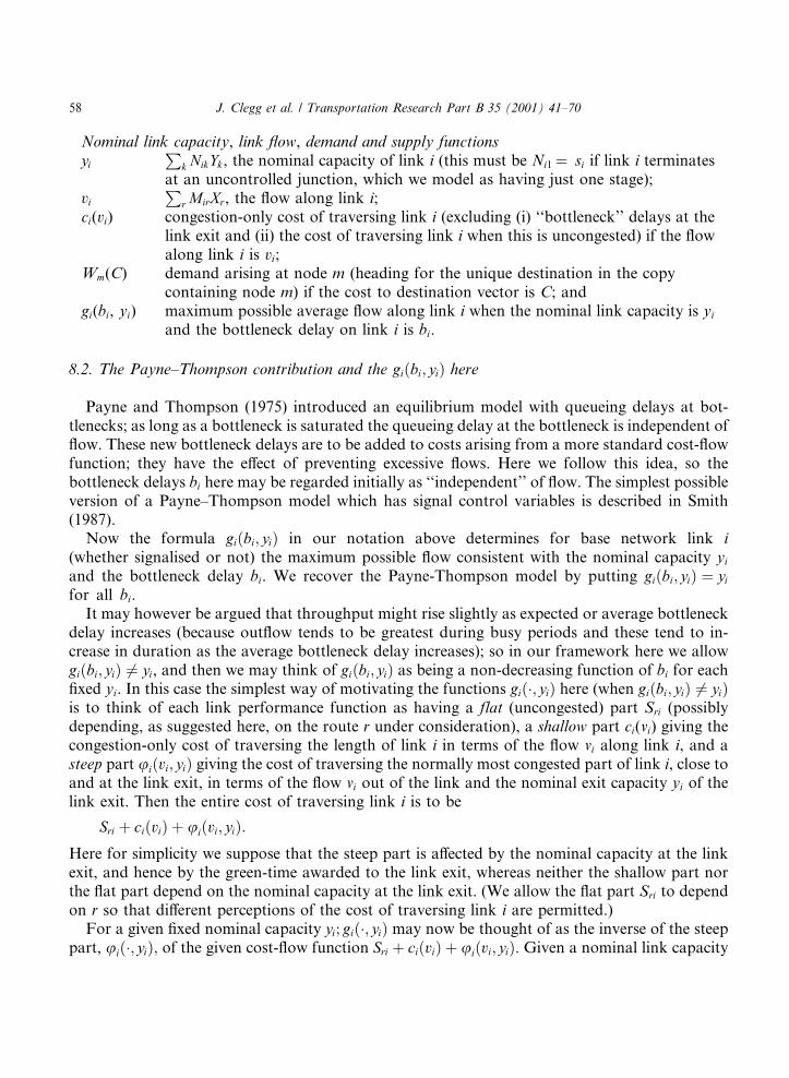
8.2. The Payne±Thompson contribution and the gi�bi; yi� here

Payne and Thompson (1975) introduced an equilibrium model with queueing delays at bot-tlenecks; as long as a bottleneck is saturated the queueing delay at the bottleneck is independent of¯ow. These new bottleneck delays are to be added to costs arising from a more standard cost-¯owfunction; they have the e�ect of preventing excessive ¯ows. Here we follow this idea, so thebottleneck delays bi here may be regarded initially as ``independent'' of ¯ow. The simplest possibleversion of a Payne±Thompson model which has signal control variables is described in Smith(1987).

Now the formula gi�bi; yi� in our notation above determines for base network link i(whether signalised or not) the maximum possible ¯ow consistent with the nominal capacity yi

and the bottleneck delay bi. We recover the Payne-Thompson model by putting gi�bi; yi� � yi

for all bi.It may however be argued that throughput might rise slightly as expected or average bottleneck

delay increases (because out¯ow tends to be greatest during busy periods and these tend to in-crease in duration as the average bottleneck delay increases); so in our framework here we allowgi�bi; yi� 6� yi, and then we may think of gi�bi; yi� as being a non-decreasing function of bi for each®xed yi. In this case the simplest way of motivating the functions gi��; yi� here (when gi�bi; yi� 6� yi�is to think of each link performance function as having a flat (uncongested) part Sri (possiblydepending, as suggested here, on the route r under consideration), a shallow part ci(vi) giving thecongestion-only cost of traversing the length of link i in terms of the ¯ow vi along link i, and asteep part ui�vi; yi� giving the cost of traversing the normally most congested part of link i, close toand at the link exit, in terms of the ¯ow vi out of the link and the nominal exit capacity yi of thelink exit. Then the entire cost of traversing link i is to be

Sri � ci�vi� � ui�vi; yi�:Here for simplicity we suppose that the steep part is a�ected by the nominal capacity at the linkexit, and hence by the green-time awarded to the link exit, whereas neither the shallow part northe ¯at part depend on the nominal capacity at the link exit. (We allow the ¯at part Sri to dependon r so that di�erent perceptions of the cost of traversing link i are permitted.)

For a given ®xed nominal capacity yi; gi��; yi� may now be thought of as the inverse of the steeppart, ui��; yi�; of the given cost-¯ow function Sri � ci�vi� � ui�vi; yi�. Given a nominal link capacity

Nominal link capacity, link ¯ow, demand and supply functionsyi

Pk NikYk, the nominal capacity of link i (this must be Ni1� si if link i terminates

at an uncontrolled junction, which we model as having just one stage);vi

Pr MirXr, the ¯ow along link i;

ci(vi) congestion-only cost of traversing link i (excluding (i) ``bottleneck'' delays at thelink exit and (ii) the cost of traversing link i when this is uncongested) if the ¯owalong link i is vi;

Wm(C) demand arising at node m (heading for the unique destination in the copycontaining node m) if the cost to destination vector is C; and

gi(bi, yi) maximum possible average ¯ow along link i when the nominal link capacity is yi

and the bottleneck delay on link i is bi.

58 J. Clegg et al. / Transportation Research Part B 35 (2001) 41±70

yi; gi�bi; yi� delivers a (largest) ¯ow vi compatible with a given end-of-link cost bi, instead ofdelivering a cost bi for each ¯ow vi: (We shall think of this end-of-link cost as ``bottleneck delay'' ±hence the letter b.)

This formulation here includes the Payne±Thompson formulation and also extends this to aformulation which allows throughput at bottlenecks to vary as average delays vary. These twomay be combined by thinking of the ``gi�bi; yi� � yi for all bi'' case as gi��; yi� being the inverse of a``vertical'' ui��; yi�. The inverse delay-¯ow or cost-¯ow functions (these are the ¯ow-delay or ¯ow-cost functions gi) may be expected to have computational advantages if the delay-¯ow or cost-¯ow function is steep or ``vertical''; because the gi are then shallow or ¯at.

8.3. User-equilibrium constraints formulated as a complementarity condition

We take Wardrop's (1952) condition: for each OD pair more costly routes carry no flow. But wechoose to write this in the following form: for each route r the cost CB�r� to the destination from thenode B(r) upstream of route r (Before r) is no more than the cost to the destination via route r,Sr � Pr �

Pi MT

ri �ci�vi� � bi�, and if it is less then no flow will enter route r, or for each route rXm

BTrmCm ÿ Sr ÿ Pr ÿ

Xi

MTri �ci�vi� � bi�6 0

and Xm

BTrmCm ÿ Sr ÿ Pr ÿ

Xi

MTri �ci�vi� � bi� < 0 implies Xr � 0:

HereP

m BTrmCm is a sum over all nodes in m in the multi-copy network; this sum just picks out one

term, CB�r�, the cost at that node (called B(r) above) at the entrance of route r. Here, for each r,Sr �

Pi Sri.

8.4. Demand constraints formulated as a complementarity condition

To ensure that the demand which arises is consistent with the travel costs we begin with thenatural assumption that for each node n the total route-flow

PrBmrXr out of node m equals the

demand Wm(C). Then we weaken this slightly to become: for each node m the total route-flowPrBmrXr out of node m is no less than the demand Wm(C) and if it is greater then Cm � 0, or: for

each m

Wm�C� ÿX

r

BmrXr6 0

and

Wm�C� ÿX

r

BmrXr < 0 implies Cm � 0:

(The sums here are over all the routes in the multi-copy network.) This is in fact, under naturalconditions (which include the Wardrop condition above), equivalent to the stronger equalitycondition.

J. Clegg et al. / Transportation Research Part B 35 (2001) 41±70 59

8.5. Capacity constraints formulated as a complementarity condition

We suppose here that for any link i with average bottleneck delay bi and nominal link capacityyi there is a maximum possible ¯ow, gi�bi; yi�, consistent with the delay bi. Then the capacityconstraint condition here becomes: the flow out of link i is no more than gi�bi; yi� and if this flow isless than gi�bi; yi� then the delay bi at the link exit is zero. In symbols this condition becomes: foreach iX

s

MisXs ÿ gi�bi; yi�6 0

and Xs

MisXs ÿ gi�bi; yi� < 0 implies bi � 0:

As speci®ed here this condition will ensure that congestion costs normally represented by the steep(or vertical) part of a cost-¯ow function will in fact occur as ``bottleneck'' delays bi which arisefrom equilibrating via the functions gi. This condition ensures that only ¯ows which ®t realisticcapacity constraints occur. Here, for each i, yi �

Pk NikYk.

8.6. A more compact formulation

First we de®ne network response functions ÿf1r;ÿf2m;ÿf3i; at each (X, C, b, Y, P),

ÿf1r�X ;C; b; Y ; P � �X

m

BTrmCm ÿ Sr ÿ Pr ÿ

Xi

MTri �ci�vi� � bi� for all r;

ÿf2m�X ;C; b; Y ; P � � Wm�C� ÿX

r

BmrXr for all m; and

ÿf3i�X ;C; b; Y ; P � �X

s

MisXs ÿ gi bi;X

k

NikYk

!for all i:

Then we rewrite the equilibrium, demand and capacity constraints above as follows:

ÿf1r�X ;C; b; Y ; P �6 0 and ÿ f1r�X ;C; b; Y ; P � < 0 implies Xr � 0;

ÿf2m�X ;C; b; Y ; P �6 0 and ÿ f2m�X ;C; b; Y ; P� < 0 implies Cm � 0;

ÿf3i�X ;C; b; Y ; P �6 0 and ÿ f3i�X ;C; b; Y ; P � < 0 implies bi � 0:

Finally we put x � �X ;C; b�; p � �Y ; P� and f �x; p� � �f1�x; p�; f2�x; p�; f3�x; p�� to obtain:x belongs to Rn

� and )f(x, p) is normal, at x, to Rn�; or

x belongs to Rn�;ÿf �x; p�6 0; and ÿfi�x; p� < 0 implies xi � 0.

(The su�x i here embraces the previous su�ces i, r and m.)These conditions are similar to a Tobin economic model and are of the form (3) or (4) above. It

remains to add the constraints:

60 J. Clegg et al. / Transportation Research Part B 35 (2001) 41±70

Zk�x; p� ÿ z6 0 for k � 1; 2; 3; . . . ;K;

rj�p�6 0 for j � 1; 2; 3; . . . ; J :

The last J inequalities include the constraints that, at each uncontrolled node the single arti®cial``stage green-time'' equals 1, and that at each signal-controlled node the sum of the stage green-times cannot exceed 1. Feasibility limits on the prices Pr are also included here. We are led toProblems P, P�n� 1� and P(2n) above.

8.7. Convexity of the n+1 functions hk in problem P�n� 1� above, for ®xed p

Convexity of the constraints for a ®xed control vector p in problem P�n� 1� ensures that ifproblem P�n� 1� is soluble then the linearised problem P�n� 1; x; p; z� is soluble for each feasible�x; p; z�. In this case, the algorithm described above is well-de®ned. Thus for our algorithm it isrelevant to determine conditions under which the n� 1 functions hk are convex for ®xed controls.

The hk in problem P�n� 1� are

ÿf1r�X ;C; b; Y ; P � �X

m

BTrmCm ÿ Sr ÿ Pr ÿ

Xi

MTri �ci�vi� � bi�;

ÿf2m�X ;C; b; Y ; P � � Wm�C� ÿX

r

BmrXr;

ÿf3i�X ;C; b; Y ; P� �X

s

MisXs ÿ gi bi;X

k

NikYk

!and

hn�1�x; p; z� � x � f �x; p�� �X ;C; b� � �ÿBTC � S � P �MT�c�v� � b�;ÿW �C� � BX ;ÿMX � g�b;NY ��� ÿX � BTC � X �MTb� C � BX ÿ b �MX � X � �S � P �MTc�v��ÿ C � W �C� � b � g�b; y�

� 0� v � c�v� ÿ C � W �C� � b � g�b; y� � X � �S � P�:It follows that all these are convex for each ®xed control vector �Y ; P� if ÿci�vi� and vici�vi� areboth convex in vi for all i, Wm(C) is convex for all nodes m in the multi-copy network and)CáW(C) is convex in C, and ÿgi�bi; yi� and bigi�bi; yi� are convex in bi for all i (for ®xed yi).

If each ci�vi� is a positive non-decreasing linear function of vi then ÿci�vi� and vici�vi� are bothconvex. If )W(C) is linear and monotone then all the Wm(C) are convex and )C�W(C) is convex.Finally, as far as the gi are concerned, consider, for example, the second term of WebsterÕs delayformula. This is equal to kvi=�yi ÿ vi� for some k > 0. For ®xed yi the inverse of this function of vi

is: gi�bi; yi� � biyi=�k � bi� for all bi. So, for ®xed yi;ÿgi�bi; yi� is a convex function of bi and alsobigi�bi; yi� is a convex function of bi. Hence the second part of Webster's delay formula has aninverse gi��; yi� such that both ÿgi�bi; yi� and bigi�bi; yi� are convex. Further, it is clear that addingtwo g's with these two desired convexity properties yields another function with the desiredconvexity properties. Of course positive linear functions satisfy both the convexity properties andso Kimber and Hollis (1979) delay formulae satisfy the convexity property as they are generated in

J. Clegg et al. / Transportation Research Part B 35 (2001) 41±70 61

precisely this manner; by adding the inverse of a function of the form kvi=�yi ÿ vi� and a positivelinear function (two functions each having the required convexity property) and then inverting thesum. Thus if the steep delay formula ui��; yi� is of Kimber and Hollis type and gi��; yi� is the inverseof ui��; yi� for ®xed yi then ÿgi�bi; yi� and bigi�bi; yi� will both be convex for ®xed yi.

9. Conclusion

The paper has outlined the need for a decision support system, implemented in software, whichmakes positive suggestions and has provided in some detail a theoretical model which may beappropriate as the basis of one such support system.

An algorithm has been outlined in which ¯ows and controls are moved so as to approachapproximate equilibrium and approximate local optimality simultaneously. We have also givencomputational results for 328 demand levels on a small network with two signalised junctions.

The method described here is currently being implemented within software but much workremains to re®ne and extend the implementation and to assess the practical e�ciency of themethod, comparing with other possible bilevel design methods.

It would be best if comparisons were made on a family of identical problems and perhaps theHai Yang network should be part of this family.

Acknowledgements

The equilibrium framework was greatly developed during a LINK project undertaken withMVA Limited and the Centre for Transport Studies at University College, London. The basiccomplementarity equilibrium condition utilised here was extensively re®ned during that LINKproject and, in particular, the section concerning the Kimber and Hollis formulae was developedduring this collaborative project.

We are grateful for the funding for the LINK project provided by DETR, ESRC and EPSRC.We are also grateful for DGVII (E2), which supported the MUSIC (Management of tra�c

USIng Control) project over three years to February 1999; and to EPSRC for consistent fundingover many years.

Finally, thanks are due to the referees whose constructive criticism has led to improvements inthe content, accuracy and style of the paper.

Appendix A. Network data for the example

In this appendix we give the data for the simple example problem concerning the networkshown in Fig. 1. Let Xr be the ¯ow along route r �r � 1; 2; 3; 4; 5�, vi be the ¯ow along link i, bi bethe cost of the bottleneck delay at the exit of link i, si be the saturation ¯ow at the exit of link i, ci

0

be the free-¯ow cost incurred in traversing link i, ci be the actual cost incurred in traversing thelength of link i (allowing for congestion along the length of the link but excluding the cost of anybottleneck delay at the link exit), and Yi be the proportion of time link i is given green�i � 1; 2; 3; 4�.

62 J. Clegg et al. / Transportation Research Part B 35 (2001) 41±70

The cost-¯ow formula used here has Sri � c0i for all i � 1; 2; 3; . . . ; 9; ci�vi� � c0

i �vi=si�2; andgi�bi; yi� � yi for all bi. This is a modi®cation of one used by Hai Yang (1996c). The bottleneckdelay ``cost'' bi experienced at the exit of link i has an important equilibrating e�ect in this net-work.

The aim is to ®nd signal green-times Yi �i � 1; 2; 3; 4� which locally minimise total travel cost,

Z � Z�X ; Y � �X

i

vi�Sri � ci�vi� � bi�;

subject to each integer rigid demand constraint: X1 � X2 � X3 � X4 � X5 � q �q � 1; 2; 3; . . . ; 328�;control constraints: Y1 � Y3 � 1; Y2 � Y4 � 1 and Yi P 0:05 �i � 1; 2; 3; 4�; capacity constraints:vi6 Yisi �i � 1; 2; 3; 4�; vi6 si �i � 5; 6; 7; 8; 9�; and user-equilibrium. (See Table 1).

Appendix B. Convergence of the algorithm

In this appendix we prove that under certain conditions every point in the limit set of the se-quence f�xn; pn; zn�g is locally e-optimal.

The main condition required involves the set of all those directions used to calculatef�xn; pn; zn�g; so let G � fd�xn; pn; zn�; n � 1; 2; 3; . . .g [ fde�xn; pn; zn�; n � 1; 2; 3; . . .g be this set.

Condition (B): The set G is bounded. That is: there is a number R such that for all i and all n theith co-ordinate di�xn; pn; zn� of d�xn; pn; zn� and the ith co-ordinate de

i�xn; pn; zn� of de�xn; pn; zn� satisfy

ÿR6 dpi �xn; pn; zn�6R and R6 de

i�xn; pn; zn�6R:

Lemma B.1. Suppose that the smoothness condition (S) holds, that f�xn; pn; zn�g is an in®nitesequence generated by the algorithm and that condition (B) holds. Suppose also that �x�; p�; z�� isin the limit set of f�xn; pn; zn�g. Then h�x�; p�; z�� ÿ e6 0.

Proof of Lemma B.1. Suppose that �x�; p�; z�� is in the limit set of f�xn; pn; zn�g and thath�x�; p�; z�� ÿ e > 0. We shall show that for all �xn; pn; zn� su�ciently close to �x�; p�; z��,

h�xn�1; pn�1; zn�1� < h�x�; p�; z��:It is clear, since Me�xn; pn; zn� is a non-increasing function of n, that this contradicts the suppositionthat �x�; p�; z�� belongs to the limit set of f�xn; pn; zn�g.

Table 1

Data for the simple example network in Fig. 1a

Link no. 1 2 3 4 5 6 7 8 9

vi � X1 X2 X3 X4 X1 � X2 X2 � X4 X1 � X 3 X 2� X 4 X5

si � 50 50 50 80 100 100 100 100 200

c0i � 4 2 3 4 4 3 4 4 15

a Note: The only di�erence between the model considered by Hai Yang and this one is that the ``shallow'' congestion-

only cost function for the length of each link i is c0i �vi=si�2 instead of c0

i �vi=Yisi�2.

J. Clegg et al. / Transportation Research Part B 35 (2001) 41±70 63

We are supposing that �x�; p�; z�� is in the limit set of f�xn; pn; zn�g and that h�x�; p�; z�� ÿ e �s > 0. Now h�xn; pn; zn� is plainly non-increasing until h6 e. It follows that h�xn; pn; zn� ÿ e P s forall n and hence

h0�xn; pn; zn� � dp�xn; pn; zn�6 ÿ s and h0�xn; pn; zn� � de�xn; pn; zn�6 ÿ s

for any chosen solution d�xn; pn; zn� of P�xn; pn; zn� and for any chosen solution de�xn; pn; zn� ofQ�xn; pn; zn�; for each n.

Hence for each n

h0�xn; pn; zn;e� � D1�xn; pn; zn� � ah0�xn; pn; zn� � dP �xn; pn; zn� � �1ÿ a�h0�xn; pn; zn� � dQ�xn; pn; zn�6 a�ÿs� � �1ÿ a��ÿs� � ÿs:

Consider moving along the line in direction D1�xn; pn; zn� from �xn; pn; zn�. Since fD1�xn; pn; zn�g isbounded and h0 is uniformly continuous, there is a positive t0 (independent of n) such that for06 t6 t0,

h0��xn; pn; zn� � tD1�xn; pn; zn�� � D1�xn; pn; zn�6 ÿ s=2 < 0:

Hence if we put H�x; p; z; t� � h��x; p; z� � tD1�x; p; z��:oH�xn; pn; zn; t�=ot � h0��xn; pn; zn� � tD1�xn; pn; zn�� � D1�xn; pn; zn�6 ÿ s=2 < 0

for all n and 06 t6 t0.Integrating oH�xn; pn; zn; t�=ot over t from 0 to t0, we deduce

H�xn; pn; zn; t0� ÿ H�xn; pn; zn; 0�6 �ÿs=2�t0:

Hence

h�xn�1; pn�1; zn�1�6H�xn; pn; zn; t0�6H�xn; pn; zn; 0� ÿ st0=2 � h�xn; pn; zn� ÿ st0=2:

Now, by continuity of h, for �xn; pn; zn� in some neighbourhood N of �x�; p�; z��h�xn; pn; zn� < h�x�; p�; z�� � st0=2:

Combining these two facts yields

h�xn�1; pn�1; zn�1�6 h�xn; pn; zn� ÿ st0=2

< h�x�; p�; z�� � st0=2ÿ st0=2 � h�x�; p�; z��;provided �xn; pn; zn� belongs to N. (There must be such an �xn; pn; zn� as we have supposed that�x�; p�; z�� is in the limit set of f�xn; pn; zn�g.)

Thus we have shown that, provided �xn; pn; zn� belongs to N,

h�xn�1; pn�1; zn�1� < h�x�; p�; z��and so, since fh�xm; pm; zm�g is non-increasing, �x�; p�; z�� cannot in fact be in the limit set off�xn; pn; zn�g. This contradiction proves that h�x�; p�; z�� ÿ e > 0 cannot hold and so h�x�; p�; z��ÿe6 0.

Lemma B.2. Under the same assumptions as stated in Lemma B.1:

Z 0�x�; p�; z�� � D1�x�; p�; z�� � 0:

64 J. Clegg et al. / Transportation Research Part B 35 (2001) 41±70

Proof of Lemma B.2. We shall show that if �x�; p�; z�� is in the limit set of f�xn; pn; zn�g andZ 0�x�; p�; z�� � D1�x�; p�; z�� < 0 then, for �xn; pn; zn� su�ciently close to �x�; p�; z��,

Z�xn�1; pn�1; zn�1� < Z�x�; p�; z��and

h�xn�1; pn�1; zn�1� ÿ e6 0:

Since Z�xn; pn; zn� is a non-increasing function of n on Ee this contradicts our assumption that�x�; p�; z�� is in the limit set of f�xn; pn; zn�g.

Accordingly suppose �x�; p�; z�� is in the limit set of f�xn; pn; zn�g and Z 0�x�; p�; z�� �D1�x�; p�; z�� < 0. We may also, by Lemma B.1, suppose Me�x�; p�; z�� � h�x�; p�; z�� ÿ e6 0.Without loss of generality we shall suppose that Me�x�; p�; z�� � h�x�; p�; z�� ÿ e � 0.

Suppose then that Me�x�; p�; z�� � h�x�; p�; z�� ÿ e � 0. Then, from the de®nition of d and de,

h0�x�; p�; z�� � d�x�; p�; z��6 ÿ e and h0�x�; p�; z�� � de�x�; p�; z��6 0:

We now move �x�; p�; z�� slightly. As both h and h0 are continuous, there is a neighbourhood N 0 of�x�; p�; z�� and a0 > 0 such that, for those �xn; pn; zn� in N 0

a�xn; pn; zn�P a0 > 0

and

h0�xn; pn; zn� � d�xn; pn; zn�6 ÿ e� a0e=2 and h0�xn; pn; zn� � de�xn; pn; zn�6 a0e=2

for any chosen solution d�xn; pn; zn� of P �xn; pn; zn� and for any chosen solution de�xn; pn; zn�.Hence for each such n

D1�xn; pn; zn� � h0�xn; pn; zn�� a�xn; pn; zn�d�xn; pn; zn� � h0�xn; pn; zn� � �1ÿ a�xn; pn; zn��de�xn; pn; zn� � h0�xn; pn; zn�6 a�xn; pn; zn��ÿe� a0e=2� � �1ÿ a�xn; pn; zn��a0e=2

� a�xn; pn; zn��ÿe� � a0e=2

6 ÿ a0e=2 � ÿh < 0:

With the above choice of N 0, consider moving along the line in direction D1�xn; pn; zn� from�xn; pn; zn� for �xn; pn; zn� 2 N 0. Since fD1�xn; pn; zn�g is bounded and h0 is uniformly continuous,there is a positive t0 such that for 06 t6 t0 and �xn; pn; zn� in N 0

h0��xn; pn; zn� � tD1�xn; pn; zn�� � D1�xn; pn; zn�6 ÿ h=2 < 0:

Hence if we put H�x; p; z; t� � h��x; p; z� � tD1�x; p; z��oH�xn; pn; zn; t�=ot � h0��xn; pn; zn� � tD1�xn; pn; zn�� � D1�xn; pn; zn�6 ÿ h=2 < 0

for 06 t6 t0 and �xn; pn; zn� in N 0.Integrating oH�xn; pn; zn; t�=ot with respect to t from 0 to t0, we deduce

H�xn; pn; zn; t0� ÿ H�xn; pn; zn; 0�6 �ÿh=2�t0:

J. Clegg et al. / Transportation Research Part B 35 (2001) 41±70 65

Hence

h�xn�1; pn�1; zn�1�6 maxfH�xn; pn; zn; t0�; eg6 maxfH�xn; pn; zn; 0� ÿ ht0=2; eg� maxfh�xn; pn; zn� ÿ ht0=2; eg:

Now, by continuity of h, for �xn; pn; zn� in some neighbourhood N 00 of �x�; p�; z��h�xn; pn; zn� < h�x�; p�; z�� � ht0=2:

Combining these two facts yields

h�xn�1; pn�1; zn�1�6 maxfh�xn; pn; zn� ÿ ht0=2; eg6 maxfh�x�; p�; z�� � ht0=2ÿ ht0=2; eg� maxfh�x�; p�; z��; eg � e:

provided �xn; pn; zn� belongs to N 0 \ N 00.Thus we have shown that under our conditions the sequence f�xn; pn; zn�g is in Ee from some

point onwards.Now we turn to Z and use similar arguments. The main assumption here is that

Z 0�x�; p�; z�� � D1�x�; p�; z�� < 0.Z 0 is continuous and so as above there is a negative number ÿu with the property that for

�xn; pn; zn� su�ciently close to �x�; p�; z�� and t su�ciently close to 0,

Z 0��xn; pn; zn� � tD1�xn; pn; zn�� � D1�x; p; z� < ÿu < 0:

Let G�xn; pn; zn; t� � Z��xn; pn; zn� � tD1�xn; pn; zn��. Then oG�xn; pn; zn; t�=ot � Z 0��xn; pn; zn��tD1�xn; pn; zn�� � D1�xn; pn; zn� < ÿu < 0. Integrating, as before, with respect to t from 0 to t0

Z�xn�1; pn�1; zn�1�6G�xn; pn; zn; t0�6 Z�xn; pn; zn� ÿ �ut0�:Now for �xn; pn; zn� su�ciently close to �x�; p�; z��

Z�xn; pn; zn� < Z�x�; p�; z�� � ut0:

Combining these two facts yields

Z�xn�1; pn�1; zn�1�6 Z�xn; pn; zn� ÿ �ut0� < Z�x�; p�; z�� � �ut0� ÿ �ut0� � Z�x�; p�; z��:Once again this shows that �x�; p�; z�� cannot belong to the limit set of our sequence as Z is non-increasing.

Thus our assumption that Z 0�x�; p�; z�� � D1�x�; p�; z�� < 0 has led to the conclusion that�x�; p�; z�� does not belong to the limit set of our sequence f�xn; pn; zn�g. This is a contradiction andshows that Z 0�x�; p�; z�� � D1�x�; p�; z�� � 0 for any point of the limit set.

Appendix C. Simultaneous feasible descent directions

Under certain conditions the existence of a feasible direction which reduces all the positive )fi

simultaneously ensures that there is a direction which reduces all positive )fi and all positive xi fi

simultaneously. The reason is monotonicity. Here we outline a proof of this initially surprisingfact.

66 J. Clegg et al. / Transportation Research Part B 35 (2001) 41±70

De®nitions and notation. Let a 2 Rn�. Then a vector v 2 Rn is said to be normal at a to Rn

� if andonly if v � �xÿ a�6 0 for all x 2 Rn

�. The set of all vectors which are normal at a to Rn� will be

denoted by N � N�a�.We shall say that a direction d in x-space is feasible at x P 0 if and only if x� d P 0. Gradients

in x-space will, for di�erentiable real-valued ui, be written: u0i.

Observation C.1. It may be veri®ed that having a single feasible descent direction for all positive ui

(say) is equivalent to: ``ÿP ciu0i is not normal at x to Rn

� for each c P 0 with at least one co-ordinate which is positive when ui > 0 and which also satis®es: ui6 0 implies ci � 0''. By thisresult, if c P 0 has at least co-ordinate which is positive when ÿfi > 0 and also has zero co-ordinates corresponding to any ÿfi6 0; then ÿP cif�ÿfi�x���g0 is not normal at x to Rn

�.Monotonicity of f now implies that, if c P 0 has at least one co-ordinate which is positivewhen �ÿfi�x��� � �xifi�x��� > 0 and also has zero co-ordinates corresponding to any �ÿfi�x��� ��xifi�x���6 0; then ÿP cif�ÿfi�x��� � �xifi�x���g0 is not normal at x to Rn

�. This is the content ofTheorem C.1 below; where for any f and any ai P 0; bi P 0 we de®ne

I � fi : aifi�a� < 0g; J � fi : ÿfi�a� < 0g and v � v�a; b� �X

J

bif0i �a� ÿ

XI

ai�xifi�0�a�:

Theorem C.1. Let f : Rn�7!Rn be monotone and di�erentiable, and a 2 Rn

�. Suppose that

bi

"� 0 for all i 62 J ;bi P 0 for all i 2 J and

XJ

bif0i �a� 2 N

#) bi � 0 for all i 2 J :

Then: {ai � 0 for all i 62 I ; ai P 0 for all i 2 I;bi � 0 for all i 62 J ; bi P 0 for i 2 J and v �Pj bif

0i �a� ÿ

PI ai�xifi�0�a� 2 N} implies ai � 0 for all i 2 I and bi � 0 for all i 2 J .

Proof of Theorem C.1. We show that, if the hypotheses of the theorem holds and if ai are zerooutside I, ai P 0 for all i 2 I , bi are zero outside J, bi P 0 for all i 2 J and not all the ai, bi are zero,then

v � v�a;b� �X

J

bif0i �a� ÿ

XI

ai�xifi�0�a�

is not normal at a to Rn�.

We do this by ®nding x 2 Rn� such that v � �xÿ a� > 0; in which case v (``based'' at a) ``looks

toward'' x. (We only need to verify this in the case that ai are not all zero since the assumptions ofthe theorem will then ensure that this is also the case if all ai are zero and all bi with i 2 J are notall zero.) So suppose that in v above the ai vanish outside I and that the ai are not all zero. Alsosuppose bi P 0 and vanish outside J and put

x � a� k

"ÿX

I

aiaiei �X

J

biei

#;

where k is a (small) positive real number. We shall show that, for an appropriately small k; x 2 Rn�

and v � �xÿ a� > 0.

J. Clegg et al. / Transportation Research Part B 35 (2001) 41±70 67

First we show that x 2 Rn�. Now I must be non-empty, ai is zero outside I and for

i 2 I; aifi�a� > 0 and so ai > 0 (otherwise aifi would be zero). Hence, for i 2 I,

xi � ai ÿ kaiai � �1ÿ kai�ai P 0 if 1ÿ kai P 0:

If, for example, we let k � minf1=ai; i 2 Ig then 1ÿ kai P 0 for all i 2 I. So we now choose k to bethis positive number and then xi P 0 for i 2 I .

Also, for this choice of k and any i 2 J ; xi � ai � kbi P ai P 0 (as a 2 Rn�; ai P 0 and also

bi P 0). Hence with our choice of k, for i 2 I and also for i 2 J ; xi P 0. It follows that x has allco-ordinates non-negative and so x 2 Rn

�.Now we show that v � �xÿ a� > 0. We have

v � ÿX

I

ai�xifi�x��0�a� �X

J

bif0i �a�

� ÿX

I

aiaif 0i �a� ÿX

I

aieifi�a� �X

J

bif0i �a�

and

xÿ a � k

"ÿX

I

aiaiei �X

J

biei

#:

Hence

�xÿ a� � v � kX

i

a2i aifi�a� ÿ k

XI

biei

!�X

J

aifi�a�ei

!

� k

ÿX

I

aiaiei �X

J

biei

!� ÿX

I

aiaif 0i �a� ÿX

J

bif0i �a�

!� kX

I

a2i aifi�a� ÿ 0

� kX

I

aif 0�a�ei

ÿX

J

bif0�a�ei

!�X

I

aiaiei

ÿX

J

biei

!

� kX

I

a2i aifi�a� � kf 0�a�

XI

aiaiei

ÿX

J

biei

!�X

I

aiaiei

ÿX

J

biei

!:

The ®rst term here is greater than 0 as, for all i 2 I; aifi�a� > 0 and at least one ai > 0. Also thesecond term has the form �Md� � d � dTMTd which must be greater than or equal to 0 as thematrix M � f 0�a� is positive semi-de®nite (since f is monotone). The proof is complete.

References

Aashtiani, H.Z., Magnanti, T.L., 1981. Equilibria on a congested transportation network. SIAM Journal of Algebraic

and Discrete Methods 2, 213±226.

68 J. Clegg et al. / Transportation Research Part B 35 (2001) 41±70

Allsop, R.E., 1974. Some possibilities for using tra�c control to in¯uence trip distribution and route choice. In:

Proceedings of the Seventh International Symposium on Transportation and Tra�c Theory, pp. 345±374.

Battye, A, Smith, M.J., Xiang, Y., 1998. The cone projection method of designing controls for transportation networks,

Mathematics in Transport Planning and Control. In: Selected Proceedings of the Third IMA International

Conference on Mathematics in Transport Planning and Control. Pergamon Press, New York, pp. 197±206.

Bazaraa, M.S., Sherali, H.D., Shetty, C.M., 1993. Nonlinear Programming ± Theory and Algorithms. Wiley, New

York, Chichester, Brisbane, Singapore.

Beckman, M., McGuire, C.B., Winsten, C.B., 1956. Studies in the Economics of Transportation. Yale University Press,

New Haven, CT.

Chiou, S-W., 1997. Optimisation of area tra�c control subject to user equilibrium tra�c assignment. In: Proceedings of

the 25th European Transport Forum, Seminar F, Volume II, pp. 53±64.

Charnes, A., Cooper, W.W., 1961. Multi-copy tra�c network models. In: Herman, R. (Ed.), Proceedings of the

Symposium on the Theory of Tra�c Flow, held at the General Motors Research Laboratories, 1958. Elsevier,

Amsterdam.

Clegg, J., Smith, M.J.,1998. Bilevel optimisation of transportation networks. In: Mathematics in Transport Planning

and Control. The Proceedings of the Third International IMA Conference on Mathematics in Transport Planning

and Control. Pergamon Press, New York, pp. 29±36.

Clune, A., Smith, M., Xiang, Y., 1999. A theoretical basis for implementation of a quantitative decision support system

± using bilevel optimisation. In: Ceder, A. (Ed.), Proceedings of the Fourteenth International Symposium on

Transportation and Tra�c Theory, Jerusalem. Pergamon Press, New York, pp. 489±514.

Dupuis, P., Nagurney, A., 1993. Dynamical systems and variational inequalities. Annals of Operations Research 24, 9±42.

Fisk, C.S., 1984. Optimal signal controls on congested networks. In: Volmuller, J., Hammerslag, R. (Eds.), Proceedings

of the Ninth International Symposium on Transportation and Tra�c Theory, Delft. VNU Science Press, Utrecht,

pp. 197±216.

Gartner, N.H., 1976. Area tra�c control and network equilibrium. In: Proceedings of the International Symposium on

Tra�c Equilibrium Methods, Montreal, 1974. Springer, Berlin, pp. 247±297.

Gauvin, J., Savard, G., 1994. The steepest descent direction for the nonlinear bilevel programming problem. Operations

Research Letters 15, 265±272.

Ghali, M.O., Smith, M.J., 1994. Comparisons of the performances of three responsive tra�c control policies, taking

drivers' day-to-day route-choices into account. Tra�c Engineering and Control 35, 555±560.

Kimber, R.M., Hollis, E.M., 1979. Tra�c queues and delays at road junctions. Transport and Road Research

Laboratory Report, 909.

Luo, Z.Q., Pang, J.S., Ralph, D., 1996. Mathematical Programs with Equilibrium Constraints. Cambridge University

Press, Cambridge.

Maher, M.J., Akcelik, R., 1975. The redistributional e�ects of an area tra�c control policy. Tra�c Engineering and

Control 16, 383±385.

Lyapunov, A.M., 1907. Probleme general de la stabilite de mouvement, Ann. Fac. Sci. Toulouse 9, 203±274. Reprinted

in Ann. Math. Stud. No 12, 1949.

Nagurney, A., Zhang, D., 1996. Projected dynamical systems and variational inequalities with applications. Kluwer

Academic Publishers, Boston, MA.

Nagurney, A., Zhang, D., 1998. Network equilibria and disequilibria, equilibrium and advanced transportation

modelling. In: Marcotte, P., Nguyen, S. (Eds.). Kluwer Academic Publishers, Boston, MA, pp. 201±243.

Outrata, J., Zowe, J., 1995. A numerical approach to optimization problems with variational inequality constraints.

Mathematical Programming 68, 105±130.

Payne, H.J., Thompson, W.A., 1975. Tra�c assignment on transportation networks with capacity constraints and

queueing. Paper presented at the 47th National ORSA/TIMS North American Meeting.

Smith, M.J., 1979a. Tra�c control and route ± choice; a simple example. Transportation Research B 13, 289±294.

Smith, M.J., 1979b. The existence uniqueness and stability of tra�c equilibria. Transportation Research B 13, 295±304.

Smith, M.J., 1979c. The marginal cost taxation of a transportation network. Transportation Research B 13, 237±242.

Smith, M.J., 1980. A local tra�c control policy which automatically maximises the overall travel capacity of an

urban road network. Paper presented at the International Symposium on Urban Tra�c Control Systems,

J. Clegg et al. / Transportation Research Part B 35 (2001) 41±70 69

Berkeley, California, August 1979). Published in the Proceedings, 11±32, and in Tra�c Engineering and Control

21, 298±302.

Smith, M.J., 1987. Tra�c control and tra�c assignment in a signal ± controlled network with queueing. In: Proceedings

of the Tenth International Symposium on Transportation and Tra�c Theory, Boston, Massachusetts. Elsevier,

Amsterdam, pp. 61±78.

Smith, M.J., Xiang, Y., Yarrow, R., 1997. Bilevel optimisation of signal timings and road prices on urban road

networks. Preprints of the IFAC/IFIP/IFORS Symposium, Crete, pp. 628±633.

Smith, M., Xiang, Y., Yarrow, R., 1998a. Descent methods of calculating locally optimal signal controls and prices in

multimodal and dynamic transportation networks. Transportation Networks: Recent Methodological Advances.

Selected Proceedings of the Fourth EURO Transportation Meeting, pp. 9±34.

Smith, M.J., Xiang, Y., Yarrow, R., Ghali, M.O., 1998b. Bilevel and other modelling approaches to urban tra�c

management and control. In: Marcotte, P., Nguyen, S. (Eds.), Equilibrium and Advanced Transportation

Modelling. Kluwer Academic Publishers, Boston, MA, pp. 283±325.

Tan, H.N., Gershwin, S.B., Athans, M., 1979. Hybrid optimization in urban transport networks. Laboratory for

information and Decision Systems, Technical Report DOT-TSC-RSPA-79-7; published by Massachusetts Institute

of Technology, Cambridge, MA, USA.

Tobin, R.L., Friesz, T.L., 1988. Sensitivity analysis for equilibrium network ¯ow. Transportation Science 22, 242±250.

Topkis, D.M., Veinott, A.F., 1967. On the convergence of some feasible direction algorithms for nonlinear

programming. SIAM J Control 5, 268±279.

Wardrop, J.G., 1952. Some theoretical aspects of road tra�c research. Proceedings Institution of Civil Engineers II 1,

235±278.

Yang, H., Yagar, S., Iida, Y., Asakura, Y., 1994a. An algorithm for the in¯ow control problem on urban freeway

networks with user ± optimal ¯ows. Transportation Research B 28, 123±139.

Yang, H., Yagar, S., 1994b. Tra�c assignment and tra�c control in general freeway ± arterial corridor systems.

Transportation Research B 28, 463±486.

Yang, H., Yagar, S., 1995. Tra�c assignment and signal control in saturated road networks. Transportation Research

A 29, 125±139.

Yang, H., 1996a. Sensitivity analysis for queueing equilibrium network ¯ow and application to tra�c control.

Mathematical and Computer Modelling 22, 247±258.

Yang, H., 1996b. Sensitivity analysis for the elastic ± demand network equilibrium problem with applications.

Transportation Research B 31, 55±70.

Yang, H., 1996c. Equilibrium network tra�c signal setting under conditions of queueing and congestion. Applications

of Advanced Technologies in transportation Engineering. In: Stephanedes, Y.J., Filippi, F. (Eds.), Proceedings of

the 4th International Conference. American Society of Civil Engineers, pp. 578±582.

Zhang, D., Nagurney, A., 1995. On the stability of projected dynamical systems. Journal of Optimisation Theory and

Applications 85, 97±124.

70 J. Clegg et al. / Transportation Research Part B 35 (2001) 41±70