
Modelling and optimising decision-making for the control of ...
199
THESE DE DOCTORAT NNT : 2022UPASB008 Modelling and optimising decision-making for the control of infectious diseases spreading on animal metapopulation networks Modélisation et optimisation de la prise de décision pour la gestion de maladies infectieuses se propageant sur des réseaux de métapopulations animales Thèse de doctorat de l’université Paris-Saclay Ecole doctorale n ◦ 581, Agriculture, Alimentation, Biologie, Environnement, Santé (ABIES) Spécialité de doctorat: Mathématiques appliquées Graduate School : Biosphera, Référent : AgroParisTech Thèse préparée dans les unités de recherche MaIAGE (Université Paris-Saclay, INRAE) et BIOEPAR (INRAE, Oniris), sous la direction de Elisabeta VERGU, Directrice de recherche, et la co-direction de Pauline EZANNO, Directrice de recherche Thèse soutenue à Paris-Saclay, le 17 mars 2022, par Lina CRISTANCHO FAJARDO Composition du jury Nicolas VAYATIS Président Professeur, ENS Paris-Saclay Ludovic MAILLERET Rapporteur & Examinateur Directeur de recherche, INRAE Centre PACA Rowland KAO Rapporteur & Examinateur Professor, University of Edinburgh Anne CORI Examinatrice Lecturer, Imperial College London Guillaume FOURNIÉ Examinateur Chercheur, Royal Veterinary College London Elisabeta VERGU Directrice de thèse Directrice de recherche, INRAE (Université Paris-Saclay) Pauline EZANNO Co-Directrice de thèse Directrice de recherche, INRAE Centre Pays de la Loire
-
Upload
khangminh22 -
Category
Documents
-
view
2 -
download
0
Transcript of Modelling and optimising decision-making for the control of ...

TH
ESE
DE
DO
CT
OR
AT
NN
T:2
022U
PASB
008
Modelling and optimising decision-makingfor the control of infectious diseasesspreading on animal metapopulation
networksModélisation et optimisation de la prise de décision pour la
gestion de maladies infectieuses se propageant sur desréseaux de métapopulations animales
Thèse de doctorat de l’université Paris-Saclay
Ecole doctorale n581, Agriculture, Alimentation, Biologie,Environnement, Santé (ABIES)
Spécialité de doctorat: Mathématiques appliquées
Graduate School : Biosphera, Référent : AgroParisTech
Thèse préparée dans les unités de recherche MaIAGE (UniversitéParis-Saclay, INRAE) et BIOEPAR (INRAE, Oniris), sous la direction deElisabeta VERGU, Directrice de recherche, et la co-direction de Pauline
EZANNO, Directrice de recherche
Thèse soutenue à Paris-Saclay, le 17 mars 2022, par
Lina CRISTANCHO FAJARDO
Composition du jury
Nicolas VAYATIS PrésidentProfesseur, ENS Paris-SaclayLudovic MAILLERET Rapporteur & ExaminateurDirecteur de recherche, INRAE Centre PACARowland KAO Rapporteur & ExaminateurProfessor, University of EdinburghAnne CORI ExaminatriceLecturer, Imperial College LondonGuillaume FOURNIÉ ExaminateurChercheur, Royal Veterinary College LondonElisabeta VERGU Directrice de thèseDirectrice de recherche, INRAE (Université Paris-Saclay)Pauline EZANNO Co-Directrice de thèseDirectrice de recherche, INRAE Centre Pays de la Loire

Titre: Modélisation et optimisation de la prise de décision pour la gestion de maladies infectieuses se propageantsur des réseaux de métapopulations animales
Mots clés: modélisation épidémiologique, réseau de métapopulation, optimisation, comportement humain, allo-cation de ressources, gestion de maladies infectieuses.
Résumé: Cette thèse porte sur la modélisation etl’optimisation de la maîtrise d’un agent pathogènese propageant dans une metapopulation d’animauxd’élevage via un réseau d’échanges commerciaux, entenant compte des processus de décision concernantl’adoption de mesures de maîtrise.
D’une part, concernant la prise de décision des éleveurs,un modèle stochastique intégrant la dynamique intra-troupeau de la maladie (composantes démographiqueset réseau d’échanges) et la dynamique des décisions deséleveurs a été développé et exploré par simulations in-tensives et analyses de sensibilité. En particulier, unmécanisme de décision dynamique qui tient comptedu comportement aléatoire des éleveurs, de leur ap-prentissage et de la dynamique d’imitation stratégiquea été proposé. Le modèle a été formalisé pour unedynamique d’infection théorique (modèle SIR), et unemesure de contrôle spécifique (vaccination). Ce premiermodèle a été étendu et adapté à une maladie réelle, laBVD (diarrhée virale bovine), où tant la transmissionde l’agent pathogène que les échanges d’informations
entre éleveurs peuvent passer par le réseau d’échanges,mais aussi par un voisinage géographique.
D’autre part, dans une perspective plus générale, il aété supposé qu’un planificateur social central cherchaità allouer dynamiquement et de manière optimale uneressource limitée entre les différentes sous-populationsd’un réseau de métapopulation donné, afin de réduirela propagation d’un agent pathogène. L’approche,basée sur des scores permettant de classer les sous-populations pour l’allocation des ressources, a été for-malisée pour le modèle épidémiologique théorique con-sidéré dans la première partie de la thèse, pour deuxmesures différentes (vaccination et traitement). Denouveaux scores ont été obtenus par l’adaptation d’uneapproche d’optimisation gloutonne au cadre des mé-tapopulations. Par le biais de simulations, les perfor-mances de ces nouveaux scores ont été comparées àcelles de plusieurs heuristiques qui pourraient être ap-propriées lorsque le réseau de métapopulation corre-spond à un réseau de commerce d’animaux.
Title: Modelling and optimising decision-making for the control of infectious diseases spreading on animalmetapopulation networks
Keywords: epidemiological modelling, metapopulation network, optimisation, human-behaviour, resource alloca-tion, infectious disease control.
Abstract: This thesis focuses on the modeling and op-timisation of the control of a pathogen spreading ina livestock metapopulation via a trade network, tak-ing into account the decision processes concerning theadoption of control measures.
On the one hand, regarding farmers’ decision-making, astochastic model integrating the intra-herd disease dy-namics (demographic components and trade network)and the dynamics of farmers’ decisions was developedand explored through intensive simulations and sen-sitivity analyses. In particular, a dynamic decision-mechanism that accounts for farmers’ random be-haviour, their learning and strategic imitation dynamicswas proposed. The model was formalised for a theo-retical infection dynamics (SIR model), and a specificcontrol measure (vaccination). This first model was ex-tended and adapted to a real-life disease, BVD (bovineviral diarrhoea), where both the pathogen spread andthe exchange of information between farmers can oc-
cur through the trade network, but also through a geo-graphical neighbourhood.
On the other hand, from a more general perspective,it was assumed that a central social planner soughtto dynamically and optimally allocate a limited re-source among the different sub-populations of a givenmetapopulation network, in order to reduce pathogenspread. The approach, based on scores allowing torank subpopulations for resource allocation, was for-malised for the theoretical epidemiological model con-sidered in the first part of the thesis, for two differentmeasures (vaccination and treatment). New scores wereobtained by adapting a greedy optimisation approach tothe metapopulation framework. Through simulations,the performances of these new scores were comparedto those of several heuristics that might be appropri-ate when the metapopulation network corresponds toan animal trade network.

Acknowledgements
In these acknowledgements I would like to thank each person that has contributed to me becom-ing a doctor and that has shaped my life in some way or another. I apologise in advance if I forgetanyone (which I probably will).
Je voudrais remercier tout d’abord mes directrices, Eliza et Pauline, qui m’ont guidé tout aulong de la thèse tant sur des questions scientifiques comme sur le plan administratif (qui n’a pasété sans complications) et qui m’ont toujours impulsé pour faire mieux. Un merci particulierpour l’encouragement pendant les confinements, la rédaction du manuscrit et la préparation dela soutenance. Merci aussi pour avoir de la confiance sur moi en me proposant de continuer àtravailler ensemble un peu plus.
I thank Ludovic Mailleret and Rowland Kao for their detailed, benevolent and constructive re-view of my thesis manuscript, which greatly helped me for the preparation of the defense. Ungrand merci aussi aux examinateurs: Anne Cori, Guillaume Fournié et Nicolas Vayatis pour fairepartie du jury pour la soutenance.
Merci aux personnes de BIOEPAR avec qui j’ai pu interagir et/ou travailler, et également auxpersonnes dans l’unité MaIAGE, l’unité où j’ai passé ces trois dernières années. En particulier,merci aux doctorants avec lesquels j’ai le plus partagé ce parcours: Romain, Henri, Léo, Ajmal,et aussi à ceux qui sont plus récemment arrivés. Merci en spécial à Romain, Henri et Madeleinede m’avoir aidé à gérer le stress de la fin de thèse.
Je voudrais aussi remercier les membres de mon comité de thèse: Nathalie Peyrard, Régis Sab-badin, Argyris Kalogeratos, Alban Thomas et Romulus Breban, pour les discussions riches et var-iées concernant l’avancement de ma thèse. Ces discussions m’ont permis de faire le point chaqueannée, ainsi que de mieux orienter mes choix scientifiques. Merci en particulier à Nathalie etRégis, qui m’ont encadrée pour mon stage de M2, grâce auquel j’ai pu confirmer mon intérêtpour faire une thèse. Plus en général, merci à toute l’unité MIAT pour tout ce que vous m’avezappris sur la France (et pas n’importe laquelle).
Merci à tous mes professeurs du M2. En particulier à Pierre Alquier et Christophe Giraud quià l’époque coordonnaient le Master Stat ML, grâce auquel j’ai compris que je voulais faire dela recherche. J’ai beaucoup apprécié votre qualité pédagogique et je vous remercie pour votreencouragement et votre aide pendant la recherche de stage et de sujet de thèse. Merci aussi à mesautres professeurs de l’ENSAE, avec qui j’ai appris énormément. En particulier merci à PierreAlquier (à nouveau), Nicolas Chopin, Arnak Dalalyan, Alexandre Tsybakov. C’était un honneurde suivre vos cours. Je remercie également tous les amis que j’ai pu me faire pendant ma scolaritéà l’ENSAE.
Merci aussi à toutes les personnes qui m’ont permis de venir en France. A l’équipe de ParisTech,en particulier à Vincent Brenier, pour avoir vu des qualités dans mon examen et mon entretien,et pour toute son aide administrative. Merci d’avoir eu confiance sur le fait que je pouvais passerd’un niveau nul en français à réussir un examen B2 en moins de 6 mois. Ce que j’ai réussi grâceà ma prof de français, Carol, qui a accepté que je rejoigne son groupe en cours de route alorsqu’elle n’était pas du tout obligée. Merci de nous avoir préparés non seulement pour l’examenmais aussi plus largement pour notre vie en France. Merci à tous mes camarades du cours defrançais qui m’ont aidée à rapidement rattraper le groupe. Gracias a las facultades de Ciencias e
3

4
Ingeniería por toda su ayuda administrativa. En particular a esta última por haber aceptado queyo siguiera la preparación al examen de ParisTech y los cursos de francés de la facultad.
Gracias a los profesores que tuve durante la carrera de estadística. A Liliana Blanco, en cuyocurso de procesos estocásticos comencé a pensar que me podía interesar la investigación y lamodelación matemática de epidemias. A Leonardo Trujillo, en especial por su recomendaciónpara la estancia de investigación en Purdue (a pesar de que finalmente decidiera venir a Eu-ropa). A Oscar Melo, por su excelente curso de diseño de experimentos, por haberme aconsejadocuando tenía dudas sobre venir a Francia, y por su recomendación para ser aceptada y becadaen el Master Statistics and Machine Learning (beca gracias a la cual pude sostenerme duranteel segundo año en Francia). Gracias también a Sergio Calderón por su ayuda en cuanto a lahomologación de materias con la UNAL. Gracias a tantos otros profesores que contribuyeron ami formación: José Alfredo Jimenez, Martha Bohorquez, German Fonseca, entre otros. Graciastambién a todas las demás personas que crucé en esta primera etapa universitaria. A mis com-pañeros y profesores de salsa y danzas afrocolombianas, con quienes aprendí que la danza podíatambién formarme como persona. Gracias en particular a mis amigos José, Emely y Adriana porlos momentos de estudio, de canto, de baile y de compartir chismes.
Gracias a los amigos que he podido hacer en Francia. A Michelle, que fue como mi mamáfrancesa durante el primer año aquí. A mis amigos colombianos: Juan, Raúl, Santiago, MariaJuliana y David, con quienes afronté el proceso de adaptación a Francia y a las grandes escuelasde ingenieros. A Juan y Raúl, por ser mi mayor soporte durante el primer año. A Juan, por suapoyo durante la thèse. A Juan y Santiago, por toda su ayuda para la soutenance.
Gracias a mis demás amigos que me quieren y apoyan desde la distancia. A mis amigas delcolegio, por las travesuras y por alegrarse tanto o incluso más que yo con mis logros académicos.Gracias en general a todas la niñas, ya mujeres, que crucé en esta etapa y para las que esperopuedan cumplir sus sueños.
Gracias a mi familia (ese batallón de tíos y tías, primos y primas), que sé que siempre me tieneen sus pensamientos. En particular, gracias a mis abuelos: Agripina, Elizabeth, Diógenes y LuisAlberto. Aunque ya no están, es gracias a ellos, quienes impulsaron sus respectivas familiasa pesar de las dificultades de la época y del contexto, que mis padres se convirtieron en losmaravillosos seres humanos que nos criaron a mí y a mis hermanos.
Merci à Sébastien, por quererme durante estos años a través de los cuales hemos crecido juntos(no en altura, ça c’est raté). Gracias por toda su ayuda y apoyo durante la thèse. Todavía mesorprende que una niñita de los Andes y un bobito d’un petit village français (encore plus petitqu’ArZacq ArraZiguet) se conocieran y encontraran en el otro a su compañero de camino. Mercià Doña Béatrice, Don Jérôme, Raphaël et Hélène de m’avoir accueillie si gentiment au sein devotre famille. Merci pour les repas, Noël, le jardinage, les balades avec les chiens, et tant d’autreschoses.
Gracias a mis hermanos y compañía. A la compañía (Sandra, José y Ale), por su apoyo constante.En particular a José, por sus relecturas (a pesar del miedo), y a mi Alejita, por ser la más ñoñade todas, en la que me veo más reflejada, y a la que espero inspirar para que haga lo que seaque le apasione. A mi hermano, César, por las relecturas también, pero sobre todo por ser mihermanito, por siempre cuidarme y hacerme la ñoña que soy. A mi hermana, Mimi, por ser mimejor amiga, y por su personalidad que me complementa.
El mayor agradecimiento de todos es para mis papás. A mi papá, William, por las madrugadasal colegio y a la universidad, por acompañarme para aquí y para allá, por ayudarme con todocuanto podía, y por acompañarme desde la distancia, pensando y rezando por mi desde quevine a Francia. A mi mamá, Miyerlandi, que es la persona más increíble e incansable que alguienpueda conocer. Ella es el motor de toda nuestra familia y de la vida de muchas personas, en par-ticular de la mía. Gracias por venir a acompañarme, cuidarme, ayudarme y soportarme durantela escritura del manuscrito, y desde siempre. Junto con mi papá hacen el mejor equipo, que nosimpulsa a actuar siempre desde la honestidad, a trazarnos grandes metas (aunque parezcan inal-canzables) y a esforzarnos por lograrlas. En especial, gracias por ‘voltear’ para que estudiáramosidiomas y expandiéramos nuestro mundo.

Contents
1 Introduction 9
1.1 Dynamic control of a disease spreading on a complex network . . . . . . . . . . . . 9
1.2 Endemic livestock diseases spreading through animal trade . . . . . . . . . . . . . 10
1.3 Main objective and structure of the thesis . . . . . . . . . . . . . . . . . . . . . . . . 12
2 State of the art and problem formulation 15
2.1 Epidemiological modelling . . . . . . . . . . . . . . . . . . . . . . . . . . . . . . . . 15
2.1.1 Compartmental models . . . . . . . . . . . . . . . . . . . . . . . . . . . . . . 16
2.1.1.1 Deterministic formalism . . . . . . . . . . . . . . . . . . . . . . . . 16
2.1.1.1.1 SIR-like models . . . . . . . . . . . . . . . . . . . . . . . . 16
2.1.1.1.2 Models with demography . . . . . . . . . . . . . . . . . . 17
2.1.1.1.3 Structured models by host-heterogeneities . . . . . . . . . 18
2.1.1.1.4 Modelling control measures . . . . . . . . . . . . . . . . . 19
2.1.1.2 Stochastic formalism . . . . . . . . . . . . . . . . . . . . . . . . . . 21
2.1.1.2.1 Event-driven approaches . . . . . . . . . . . . . . . . . . . 21
2.1.1.2.2 Simulation of stochastic models . . . . . . . . . . . . . . . 22
2.1.1.2.3 Measures of persistence . . . . . . . . . . . . . . . . . . . 23
2.1.1.3 Generalisation of classic hypotheses in epidemiological modelling 23
2.1.2 Spatial structure in epidemiological models . . . . . . . . . . . . . . . . . . . 24
2.1.3 Network epidemiology . . . . . . . . . . . . . . . . . . . . . . . . . . . . . . 25
2.1.3.1 Static networks . . . . . . . . . . . . . . . . . . . . . . . . . . . . . . 25
2.1.3.1.1 Network connectivity measures . . . . . . . . . . . . . . . 26
2.1.3.1.2 Network models for complex networks . . . . . . . . . . 27
2.1.3.2 Dynamic networks . . . . . . . . . . . . . . . . . . . . . . . . . . . 28
2.1.3.3 Infection dynamics on metapopulation networks . . . . . . . . . . 29
2.1.3.4 Infection dynamics on animal trade networks . . . . . . . . . . . . 30
2.2 Decision-making with application in epidemiology . . . . . . . . . . . . . . . . . . 30
2.2.1 Types of decision problems . . . . . . . . . . . . . . . . . . . . . . . . . . . . 31
2.2.2 Decentralised decision-making: modelling human behaviour . . . . . . . . 32
2.2.2.1 Phenomenological models . . . . . . . . . . . . . . . . . . . . . . . 32
2.2.2.2 Psychological models . . . . . . . . . . . . . . . . . . . . . . . . . . 33
5

6 CONTENTS
2.2.2.3 Classical game theory . . . . . . . . . . . . . . . . . . . . . . . . . . 34
2.2.2.4 Evolutionary game theory . . . . . . . . . . . . . . . . . . . . . . . 35
2.2.2.5 Reinforcement Learning . . . . . . . . . . . . . . . . . . . . . . . . 37
2.2.3 Centralised decision-making: optimising the system . . . . . . . . . . . . . 40
2.2.3.1 Control levers and practical considerations . . . . . . . . . . . . . 40
2.2.3.2 Allocation problems . . . . . . . . . . . . . . . . . . . . . . . . . . . 41
2.2.3.3 Control approaches . . . . . . . . . . . . . . . . . . . . . . . . . . . 41
2.2.3.3.1 Spectral control . . . . . . . . . . . . . . . . . . . . . . . . 42
2.2.3.3.2 Optimal control theory . . . . . . . . . . . . . . . . . . . . 42
2.2.3.3.3 Markov decision processes . . . . . . . . . . . . . . . . . . 43
2.2.3.3.4 Score-based approaches . . . . . . . . . . . . . . . . . . . 43
2.3 Decision-making regarding the control of disease spread on a trade network:problem formulation and selected approaches . . . . . . . . . . . . . . . . . . . . . 44
3 Accounting for farmers’ control decisions in a model of pathogen spread through ani-mal trade 49
3.1 Introduction . . . . . . . . . . . . . . . . . . . . . . . . . . . . . . . . . . . . . . . . . 50
3.2 Integrative model . . . . . . . . . . . . . . . . . . . . . . . . . . . . . . . . . . . . . . 51
3.2.1 Epidemic model with demography in a metapopulation based on a tradenetwork . . . . . . . . . . . . . . . . . . . . . . . . . . . . . . . . . . . . . . . 51
3.2.2 Farmers’ decision-making model . . . . . . . . . . . . . . . . . . . . . . . . . 54
3.2.3 An epidemic control measure . . . . . . . . . . . . . . . . . . . . . . . . . . . 56
3.2.4 An economic-epidemiological cost function . . . . . . . . . . . . . . . . . . . 57
3.3 Setting for simulations and sensitivity analyses . . . . . . . . . . . . . . . . . . . . . 58
3.3.1 Fixed simulation setting . . . . . . . . . . . . . . . . . . . . . . . . . . . . . . 58
3.3.2 Parameters of the integrative model . . . . . . . . . . . . . . . . . . . . . . . 64
3.3.3 Sensitivity analysis experiments . . . . . . . . . . . . . . . . . . . . . . . . . 64
3.4 Results of the simulation study and sensitivity analyses . . . . . . . . . . . . . . . . 66
3.4.1 Model predictions for different decision scenarios . . . . . . . . . . . . . . . 66
3.4.2 Key determinant parameters of decision-making and epidemiological dy-namics . . . . . . . . . . . . . . . . . . . . . . . . . . . . . . . . . . . . . . . . 74
3.5 Discussion . . . . . . . . . . . . . . . . . . . . . . . . . . . . . . . . . . . . . . . . . . 76
4 Dynamic resource allocation for controlling pathogen spread on a large metapopulationnetwork 79
4.1 Introduction . . . . . . . . . . . . . . . . . . . . . . . . . . . . . . . . . . . . . . . . . 80
4.2 Dynamic resource allocation in the metapopulation framework . . . . . . . . . . . 81
4.3 Score-based strategies . . . . . . . . . . . . . . . . . . . . . . . . . . . . . . . . . . . 82
4.3.1 Greedy scores . . . . . . . . . . . . . . . . . . . . . . . . . . . . . . . . . . . . 82
4.3.2 Heuristic scores . . . . . . . . . . . . . . . . . . . . . . . . . . . . . . . . . . . 84
4.4 Simulation setting and numerical explorations . . . . . . . . . . . . . . . . . . . . . 84

CONTENTS 7
4.4.1 Setting for the exploration of infection-related dynamics with score-basedresource allocation . . . . . . . . . . . . . . . . . . . . . . . . . . . . . . . . . 84
4.4.2 Setting for percolation analysis . . . . . . . . . . . . . . . . . . . . . . . . . . 86
4.5 Results . . . . . . . . . . . . . . . . . . . . . . . . . . . . . . . . . . . . . . . . . . . . 87
4.5.1 Greedy scoring functions . . . . . . . . . . . . . . . . . . . . . . . . . . . . . 87
4.5.2 Results of numerical explorations . . . . . . . . . . . . . . . . . . . . . . . . 88
4.5.2.1 Infection-related dynamics following score-based resourceallocation . . . . . . . . . . . . . . . . . . . . . . . . . . . . . . . . . 88
4.5.2.2 Percolation analysis results . . . . . . . . . . . . . . . . . . . . . . . 95
4.6 Discussion . . . . . . . . . . . . . . . . . . . . . . . . . . . . . . . . . . . . . . . . . . 102
4.7 Appendix: Analytical derivation of the greedy scoring functions . . . . . . . . . . . 105
4.7.1 Vaccination . . . . . . . . . . . . . . . . . . . . . . . . . . . . . . . . . . . . . 106
4.7.1.1 Minimise a function of the number of infected herds . . . . . . . . 106
4.7.1.2 Minimise a function of the total number of infected animals . . . . 109
4.7.2 Treatment . . . . . . . . . . . . . . . . . . . . . . . . . . . . . . . . . . . . . . 110
4.7.2.1 Minimise a function of the number of infected herds . . . . . . . . 110
4.7.2.2 Minimise a function of the total number of infected animals . . . . 114
5 Application study: Learning and strategic imitation in modelling farmers’ dynamic de-cisions on BVD vaccination 117
5.1 Introduction . . . . . . . . . . . . . . . . . . . . . . . . . . . . . . . . . . . . . . . . . 117
5.2 The BVD model . . . . . . . . . . . . . . . . . . . . . . . . . . . . . . . . . . . . . . . 118
5.2.1 Data description . . . . . . . . . . . . . . . . . . . . . . . . . . . . . . . . . . 118
5.2.2 Within-herd epidemiological-demographic dynamics . . . . . . . . . . . . . 122
5.2.2.1 Life-cycle and health-state dynamics . . . . . . . . . . . . . . . . . 122
5.2.2.2 Handling trade movements . . . . . . . . . . . . . . . . . . . . . . 128
5.2.2.3 Epidemiological effect of vaccination . . . . . . . . . . . . . . . . . 129
5.3 Farmer’s decision-making on vaccination . . . . . . . . . . . . . . . . . . . . . . . . 129
5.3.1 Decision-mechanism . . . . . . . . . . . . . . . . . . . . . . . . . . . . . . . . 129
5.3.2 Economic-epidemiological cost . . . . . . . . . . . . . . . . . . . . . . . . . . 131
5.4 Simulation setting . . . . . . . . . . . . . . . . . . . . . . . . . . . . . . . . . . . . . . 133
5.5 Results . . . . . . . . . . . . . . . . . . . . . . . . . . . . . . . . . . . . . . . . . . . . 134
5.6 Discussion . . . . . . . . . . . . . . . . . . . . . . . . . . . . . . . . . . . . . . . . . . 140
6 Conclusions and perspectives 143
6.1 Main contributions . . . . . . . . . . . . . . . . . . . . . . . . . . . . . . . . . . . . . 143
6.1.1 Integrative model for pathogen spread over an animal trade network ac-counting for farmers’ dynamic decisions regarding the adoption of a healthmeasure . . . . . . . . . . . . . . . . . . . . . . . . . . . . . . . . . . . . . . . 144
6.1.2 Strategies for the dynamic resource allocation of a limited resource for con-trolling disease spread on a metapopulation network . . . . . . . . . . . . . 144

8 CONTENTS
6.1.3 Study on farmers’ vaccination decisions integrated in a model of BVD’sspread at a large scale . . . . . . . . . . . . . . . . . . . . . . . . . . . . . . . 145
6.2 Perspectives . . . . . . . . . . . . . . . . . . . . . . . . . . . . . . . . . . . . . . . . . 145
6.2.1 On decentralised decision-making . . . . . . . . . . . . . . . . . . . . . . . . 145
6.2.1.1 Noisy observation of costs . . . . . . . . . . . . . . . . . . . . . . . 145
6.2.1.2 Variations of the decision-making algorithm . . . . . . . . . . . . . 146
6.2.1.3 Robustness to parameter values . . . . . . . . . . . . . . . . . . . . 146
6.2.1.4 More relevant field measures . . . . . . . . . . . . . . . . . . . . . . 147
6.2.2 On centralised decision-making . . . . . . . . . . . . . . . . . . . . . . . . . 147
6.2.2.1 Noisy or partial health information . . . . . . . . . . . . . . . . . . 147
6.2.2.2 Sub-network . . . . . . . . . . . . . . . . . . . . . . . . . . . . . . . 148
6.2.2.3 Dynamic network . . . . . . . . . . . . . . . . . . . . . . . . . . . . 148
6.2.3 On decentralised and centralised decision-making . . . . . . . . . . . . . . . 148
6.2.3.1 Coupled centralised-decentralised decision-making . . . . . . . . 148
6.2.3.2 Decision-step optimisation: when to allocate? . . . . . . . . . . . . 149
6.3 Conclusion . . . . . . . . . . . . . . . . . . . . . . . . . . . . . . . . . . . . . . . . . . 149
7 Résumé en français: contexte et contributions de la thèse 151
7.1 Contexte . . . . . . . . . . . . . . . . . . . . . . . . . . . . . . . . . . . . . . . . . . . 151
7.1.1 Gestion dynamique de la propagation d’une maladie sur un réseau complexe151
7.1.2 Maladies endémiques du bétail se propageant par le biais du commerce desanimaux . . . . . . . . . . . . . . . . . . . . . . . . . . . . . . . . . . . . . . . 153
7.2 Contributions . . . . . . . . . . . . . . . . . . . . . . . . . . . . . . . . . . . . . . . . 155
7.2.1 Modèle intégratif pour la propagation d’agents pathogènes sur un réseaude commerce d’animaux rendant compte des décisions dynamiques desagriculteurs concernant l’adoption d’une mesure sanitaire . . . . . . . . . . 155
7.2.2 Stratégies pour l’allocation dynamique d’une ressource limitée pour la ges-tion de la propagation des maladies sur un réseau de métapopulation . . . 156
7.2.3 Etude sur les décisions de vaccination des agriculteurs intégrées dans unmodèle de propagation de la diarrhée virale bovine à grande échelle . . . . 157
7.3 Conclusion . . . . . . . . . . . . . . . . . . . . . . . . . . . . . . . . . . . . . . . . . . 157

Chapter 1
Introduction
1.1 Dynamic control of a disease spreading on a complexnetwork
The structure of contacts between individuals is a key element to account for to better understandthe spread of infectious diseases, and ultimately to control it (Keeling et al. 2005). This is partic-ularly true for disease transmission between several sub-populations on a large geographic area.Although pathogens can be transmitted between sub-populations in several ways, depending onthe particular pathogen and context (e.g. shared environment, wild-animal vectors), one of themost usual paths for transmission occurs through the movement of infected individuals (Danonet al. 2011).
Indeed, the movements of individuals between different sub-populations form a network struc-ture in which the sub-populations are interconnected by the movement links, called a metapop-ulation network (Keeling et al. 2005). Such a network is directed, as individuals move from onesub-population to another; weighted, as there is a weight (flow of individuals) associated witheach link; and dynamic, as flows change over time (different movement connections and differ-ent amounts of individuals). Furthermore, when spatial coordinates are explicitly considered,the links can connect sub-populations even if there is no geographical proximity between them(spatial network).
In particular, this context allows to describe two specific phenomena. First, the introduction of apathogen in a sub-population where it was not present, known as a colonisation event (Donahueet al. 2008). The second type of phenomenon is the persistence of pathogen propagation at largescale despite fade-out at small scale, which is known as a rescue effect (Brown et al. 1977). Thisis a well known concept in ecology: there are short-lived epidemics at the sub-population level,but the disease is maintained at a large scale due to interactions among sub-populations.
The question of controlling a disease spreading on such a complex network rapidly emerges(Enright et al. 2018). The system is intrinsically dynamic (due to the movements of individu-als, demographic changes in the sub-populations over time, and disease spread), as can be thedecision-making. Indeed, real-life control of infectious diseases is usually conducted throughrepeated decisions over time (vaccine campaigns, temporal movement restrictions, etc.).
Moreover, given the fact that the network is large and encompasses many sub-populations, thedecisions regarding the adoption of control measures to reduce the disease spread can be takenat two different levels. On the one hand, if there is a human decision-making agent associatedto each sub-population of the system, we are concerned with decentralised human decision-making.On the other hand, the management can be carried out by a central planner, usually a social plan-ner. This is referred to as centralised social-planner decision-making. The distinction between thesetwo types of decision-making is important since depending on the decision-maker, decisionswould respond to different motivations. Furthermore, decentralised human decision-making
9

10 CHAPTER 1. INTRODUCTION
can naturally introduce strategic behaviour and heterogeneous implementation of control mea-sures among the many sub-populations of the system (Kreps 1997).
In this context, the use of suitable mathematical approaches is really helpful and strongly recom-mended for describing and controlling such a system. In particular, mechanistic epidemiologicalmodels can be useful instruments to represent and understand the complex system involvedin pathogen spread (Keeling et al. 2011). Since human behaviour can have a major role in thespread of diseases, especially for those whose control is voluntary, taking into account decision-making related to controlling the spread can increase the accuracy of these models, in terms ofunderstanding and prediction. Furthermore, on the basis of these mechanistic models, strate-gies can be designed for controlling the propagation of the disease (Manfredi et al. 2013). Yet, inthe process of modelling and controlling such a system, crucial methodological challenges arisewhen accounting for dynamic decision-making, either made by a social-planner or by the humanagents in the system.
Though mathematical mechanistic modelling is increasingly being used in the study of infectiousdiseases, most existing models in literature do not refer to voluntary decisions of interactingagents (Wang et al. 2016), or they do not consider that the decision-making process is dynamic(Rat-Aspert et al. 2010). Furthermore, classical approaches either consider humans as particles(Manfredi et al. 2013), or when economic aspects are taken into account agents are considered tobe perfectly rational (e.g. Bauch et al. 2004; Zhang et al. 2012), which is a strong and controversialhypothesis for human decision-making (Wang et al. 2016). Finally, influences between agentsdecisions are often neglected (Shi et al. 2019), despite the fact that it is an important feature ofhuman behaviour, particularly regarding the management of livestock diseases (Hidano et al.2018).
Hence, from a modelling perspective, a first challenge consists in building a framework thatappropriately formalises the relation between the dynamics of a disease spreading on a largemetapopulation network, and the dynamics of the voluntary adoption of control measures ineach sub-population, while accounting for relevant psychological, cognitive or economic consid-erations.
A second challenge consists in developing or adapting methods that can effectively be appliedfor optimally controlling the spread of the disease on the network. Among the considerations tobe taken into account, one of the most important should be of computational nature. Indeed, thisis the major challenge for solving an optimisation problem in the present framework, due to thelarge dimension of the network (Pellis et al. 2015).
For this reason, research on this matter has mostly been focused on two types of situations: ei-ther the network is small (e.g. Chernov et al. 2020; Viet et al. 2018), or it is a large network ofindividuals, i.e. not a meta-population (e.g. Lorch et al. 2018; Zhang et al. 2015). In the first case,studies are mostly based on Markov Decision processes (MDP) (Puterman 2014) or game-theory(Myerson 1997). In the second one, authors usually recur to mean-field approximations inspiredfrom physics (Lasry et al. 2007), which can be inappropriate if one wishes to account for limitedrationality or heterogeneities among agents. For example, this can concern the influence thatan agent may have on other agents’ decisions, which can be determined by their place in thenetwork.
The expected advances from these two perspectives, modelling and optimisation, can contributeto better understand and take into account different characteristics of the complex system in-volved in pathogen spread on such a network, and ultimately to effectively control it.
1.2 Endemic livestock diseases spreading through animal trade
In essence, the transmission of a disease does not much differ whether the individuals are hu-mans or animals (wildlife or livestock), yet they present some differences. First, humans tendto move freely between households, work places, study places, cities, countries, etc. while live-stock are usually in one farm for a long time before going to another one through animal trade

1.2. ENDEMIC LIVESTOCK DISEASES SPREADING THROUGH TRADE 11
(Brooks-Pollock et al. 2015). Second, economic considerations can be more central for the con-trol of livestock diseases than for human diseases, where the public health aspect generally takesprecedence over the rest. Hence, methodological advances for controlling the first are in principlemore likely to find the compliance of field agents.
Following the crisis on bovine spongiform encephalopathy (commonly known as mad cow dis-ease) that took place particularly in the United Kingdom between 1986 and 2000, European coun-tries maintain national databases regarding cattle movements between farms. Indeed, animalmovements caused by trading are a major path on which livestock pathogens can be transmittedbetween holdings (Fèvre et al. 2006), e.g. paratuberculosis (Beaunée et al. 2015), foot-and-mouthdisease (FMD) (Ferguson et al. 2001) and bovine tuberculosis (bTB) (Donnelly et al. 2003).
These exchanges occur directly between two farms, or can pass through intermediate structures.The first ones generally concern farms that are geographically close, so the disease spread ismostly concentrated in a small geographic area. Also, animal movements can occur via mar-kets or assembling centres. These structures facilitate animal trade at a large geographical scale,increasing exchanges of animals that come from a holding that is geographically far from thedestination holding. Hence, they further increase the transmission risk of pathogens over largeareas (Robinson et al. 2007). Figure 1.1 illustrates the example of a cattle trade network formed bythe dairy animal movements between cattle herds, that occurred in 2009 in France based on theFrench cattle identification database (FCID), which records the life history of each cattle animalfrom birth to death. This figure evidences geographically close and far animal exchanges thatcan take place in an animal trade network, and through which a disease spread is susceptible toattain the whole French territory.
Figure 1.1: Cattle trade flows (dairy animals only) for year 2009 in France, based on the French cattle identi-fication database. Each node is a commune (the smallest French administrative unit). Source: Gaël Beaunée.
A disease spreading though animal exchange has high chances of becoming endemic in a givenarea, i.e. present at a given (generally moderate) prevalence in the whole population for longperiods of time (Carslake et al. 2011). As mentioned for the general metapopulation setting, inanimal metapopulations disease persistence can be observed at large scale by the means of twoprocesses. First, a long infection duration in a sub-population gives rise to long metapopulationinfection. Second, persistence can be observed if there is a rescue effect due to interactions amongsub-populations (see for example Jesse et al. 2008).
Alternatively, a disease can exhibit epidemic dynamics, which by definition means that a largeand rapid spread in a short period of time is observed. Examples of this type are FMD (Fergusonet al. 2001), African swine fever (ASF) (Nigsch et al. 2013), and avian influenza (Benincà et al.

12 CHAPTER 1. INTRODUCTION
2020). For a given disease, the distinction between endemic and epidemic dynamics is madeusing surveillance data. Yet, detailed surveillance data is mainly available for diseases that havealready been labelled as epidemics (Carslake et al. 2011).
Once a disease is associated to an epidemic dynamics, significant political efforts are made inorder to eradicate it. In particular, public policies generally target livestock epidemic diseases byregulating their control in a mandatory manner. In that case, it is said that the disease is regulated.Meanwhile, endemic diseases are generally of less interest to public opinion and policy-makers.Hence, their control is often left to individual or local initiatives, and is therefore not mandatory,causing endemic diseases to be most often unregulated.
Nevertheless, as they persist over long time periods, endemic diseases can have a large cumu-lative incidence, leading to a reduction in farms economic profitability and in animal welfare(Tomley et al. 2009). Furthermore, zoonotic diseases (i.e. infectious diseases that have jumpedfrom animals to humans) play a major role in the increasing number of human emerging dis-eases (Lefrançois et al. 2014). Indeed, at least 60% of human emerging infectious diseases arezoonotic, and in particular over 30% of emerging infectious zoonotic diseases are associated withfood animals (Otte et al. 2021). Hence, the control of livestock endemic diseases represents a ma-jor challenge for animal health and for sustainable agrifood systems, particularly in a context ofsub-populations that trade animals, and of endemic diseases for which control is not compulsory.
Decision-making for the adoption of one or several health measures is therefore of interest forassessing the control of animal endemic diseases. As farmers production objectives are not onlydriven by animal health but also by criteria of working time, productivity, profitability, etc, theheterogeneity of the measures implementation is increased (Ezanno et al. 2020). For example, acentral decision-maker may decide to isolate a herd if this implies an overall reduction in disease,provided that this is the objective. However, if the farmers themselves decide whether or not toisolate their herd, they will rather make this decision solely on the basis of their own criteria,which is generally not optimal at the collective level (Krebs et al. 2018).
For unregulated diseases, it is natural to think that decisions concerning herd management aremade mostly by the farmers themselves. Yet, decisions on control measures can also be taken at acentralised level, even if only by local organisations composed of several farmers. In some Frenchadministrative areas, for example, animal health services (GDS: groupement de défense sanitaire)may engage in various types of control actions to reduce the local disease prevalence. Theseactions may involve, for example, the allocation of health resources for intervening in the systemwithout requiring all farmers to implement the measure, or the use of campaigns to encourage thevoluntary adoption of the measure by farmers. Intervention can also be achieved by facilitatingaccess to information on the infection-related status of herds, so that farmers can make moreinformed, and possibly better, decisions.
Moreover, many control or prevention measures are possible (application of vaccines or treat-ments, testing and culling of positive animals, isolation of infected animals, etc.). It can be dif-ficult to choose, either from the farmer or the social planner point of view, among the differentoptions whose effectiveness is not always known or comparable. Furthermore, anticipating theimpact of these individual or collective choices on the large-scale dynamics of infectious diseasesremains a challenge.
1.3 Main objective and structure of the thesis
The main objective of this thesis was to identify, adapt and build the suitable approaches foreffectively model and optimise the adoption of control measures for limiting a disease spreadingon a large metapopulation network. The network was specifically considered to be a livestocktrade network through which the disease can spread over a certain region.
The manuscript is structured in the following manner. This introductory chapter is followedby Chapter 2, that presents the state of the art on epidemiological modelling, particularly onnetworks, and on decision-making approaches in systems with several individuals. These two

1.3. MAIN OBJECTIVE AND STRUCTURE OF THE THESIS 13
categories of modelling approaches are put together for selecting the suitable elements that areused in the rest of the thesis.
Chapter 3 addresses the modelling challenge, through the development of a new integrativemechanistic model, with a feedback loop between the dynamics of a (theoretical) pathogen spread-ing on an animal trade network, and the decision-making of farmers regarding the voluntaryapplication of control measures. The decision process is governed by a stochastic algorithm. Thework in this chapter was published in Scientific Reports in 2021 (Cristancho Fajardo et al. 2021).
For the optimisation challenge, in Chapter 4, the point of view is the one of a single social plannerdistributing a limited resource aimed at reducing the spread of a (theoretical) disease on thenetwork. At first, the focus is on the construction of optimised indicators to target the nodes of ametapopulation network. Then, the performances of these analytical scores are explored as wellas those of relevant heuristic indicators, from an epidemiological and feasibility point of view.This chapter has been published in the Journal of the Royal Society Interface (Cristancho-Fajardoet al. 2022).
Chapter 5 presents a new variant of the decision making algorithm as an extension of the modeldeveloped in Chapter 3, with application to a specific disease, the bovine viral diarrhoea (BVD).Here, farmers exchange information relative to their decisions either through the trade network,or through a geographic proximity network.
The final chapter (Chapter 6) summarises the developed methods and contributions, discussestheir relevance and limitations, and presents some perspectives on the basis of this thesis work,for the control of diseases spreading on metapopulation networks.


Chapter 2
State of the art and problemformulation
Contents2.1 Epidemiological modelling . . . . . . . . . . . . . . . . . . . . . . . . . . . . . . 15
2.1.1 Compartmental models . . . . . . . . . . . . . . . . . . . . . . . . . . . . . 162.1.2 Spatial structure in epidemiological models . . . . . . . . . . . . . . . . . 242.1.3 Network epidemiology . . . . . . . . . . . . . . . . . . . . . . . . . . . . . 25
2.2 Decision-making with application in epidemiology . . . . . . . . . . . . . . . . 302.2.1 Types of decision problems . . . . . . . . . . . . . . . . . . . . . . . . . . . 312.2.2 Decentralised decision-making: modelling human behaviour . . . . . . . 322.2.3 Centralised decision-making: optimising the system . . . . . . . . . . . . 40
2.3 Decision-making regarding the control of disease spread on a trade network:problem formulation and selected approaches . . . . . . . . . . . . . . . . . 44
This thesis relies on two main topics: epidemiological modelling and decision-making appliedto epidemiology. In this chapter, I present a non-exhaustive state of the art on these two topics(sections 2.1 and 2.2, respectively), focusing on the mathematical ingredients that could address(or be involved in) the challenges presented in section 1.3. Finally, some choices regarding suchingredients are made in section 2.3 to be integrated to approaches developed in the followingchapters.
2.1 Epidemiological modelling
In epidemiology, mathematical models are used to describe the spread of infectious diseases in aformalised manner. The first known such mathematical model is attributed to Daniel Bernoulliin 1760 (Hethcote 2000). The next registers of mathematical epidemiological models appear inthe XX century, through the works of Hamer 1906 for measles, and Ross 1910 on malaria. Inparticular, Hamer’s work introduces the law of mass action into epidemiology, consisting in theidea that the number of new infections within a population is proportional to the number ofinfected and susceptible individuals. This law implicitly assumes that the population verifies thehomogeneous mixing hypothesis, so the contact rate between two individuals is the same for anypair of them. The work of Hamer and Ross, as well as that of Kermack and McKendrick in the1920s, constitute the basic models for describing the spread of infectious diseases: compartmentalmodels. Then, in the mid-1980s, the work of Klovdahl 1985 and May et al. 1987 paved the wayfor the developement of connections between epidemiology and network theory (Danon et al.2011).
15

16 CHAPTER 2. STATE OF THE ART AND PROBLEM FORMULATION
2.1.1 Compartmental models
Compartmental models consist in dividing the population into homogeneous compartments,according to their health status regarding the disease. Each compartment contains the number(proportion) of the individuals in a given state. Their evolution over time is described by adynamical system.
From the point of view of the mathematical formalism, models can be deterministic or stochastic,even if their compartmental structure is the same. Although the spread of infectious diseases isstochastic, as it is influenced by many random factors, deterministic models are widely used. Inparticular, when the stochasticity is only related to the population size, and this one is large, itcan be neglected by using a deterministic model. Indeed, for such type of intrinsic stochasticity,(and under certain conditions) the deterministic formulation corresponds to the large populationlimit of the stochastic formulation (Britton et al. 2019).
In the following, for simplicity reasons, I use the deterministic formalism for describing the maintypes of structures that compartmental models can present.
2.1.1.1 Deterministic formalism
Most deterministic models are represented by ordinary differential equations (ODE) and cantherefore be simulated using numerical schemes such as the Euler method (Euler 1794), the sim-plest algorithm yet not the best one (Keeling et al. 2011).
2.1.1.1.1 SIR-like models The first simple compartmental model is the SIR model of Kermacket al. 1927. In this model, the population is divided into three compartments: the susceptible (S),the infected (I), and the recovered (R) compartments. In the most basic form of the model, theonly two possible transitions are: getting infected (going from the S to the I compartment), orrecovering (going from I to R). In its deterministic form, the SIR model can be mathematicallywritten through the following ODE:
dS(t)
dt= −λ(t)S(t),
dI(t)
dt= λ(t)S(t)− γI(t),
dR(t)
dt= γI(t).
(2.1)
S(t), I(t) and R(t), are the numbers of susceptible, infected and recovered individuals at timet. The usual initial conditions of the system described by the previous equations are S(0) >0, I(0) > 0 and R(0) = 0. The parameter γ is the self-recovery rate, and can be defined as theinverse of the mean duration of the infectious period. This constant recovery rate, independentfrom the time since infection, implies that the infectious period follows an exponential distribu-tion in the stochastic setting (see section 2.1.1.3 for a discussion on this hypothesis).
The force of infection λ(t) is defined as the per capita rate at which a susceptible individual con-tracts the infection, so λ(t)S(t) is the rate at which new infections are produced in the population.The model is represented in figure 2.1.
S I Rλ γ
Figure 2.1: SIR flow diagram. λ(t) is the force of infection and γ is the recovery rate.
Concerning the form of λ(t) two options are mostly used (McCallum et al. 2001). First, one canassume density-dependence, where the contact rate between individuals depends on the size of

2.1. EPIDEMIOLOGICAL MODELLING 17
the population, N(t), and therefore the rate at which new infections take place depends on thedensity of infected individuals, I(t). So λ(t) = βI(t), where β accounts for the product betweenthe contact rate of a susceptible and an infected individual, and the probability of transmissionfollowing contact. On the contrary, it is possible to suppose that the transmission is frequency-dependent, where the contact rate does not depend on the size of the population, so the newinfections depend on the proportion of infected individuals rather than on their density. In thiscase λ(t) = βI(t)/N(t). The choice of one of the two hypotheses will be important if N(t) showsgreat variation over time, otherwise 1/N(t) can be considered as a multiplicative factor of theβ coefficient. Indeed, it is often assumed that the size of the population is constant in time, inwhich case both functions are proportional, i.e. N(t) = N = S(t) + I(t) + R(t),∀t. In othercases, when population size varies over time, there is no absolute way to know if, for an applica-tion, the density-dependence or the frequency-dependence is the more appropriate hypothesis.Yet, frequency-dependence is most often assumed for human diseases, since usually there aresimilar social patterns between individuals irrespective of N . Meanwhile, density-dependenceis more often assumed for animal diseases, as animals might be more crowded in the same ge-ographical area, which would increase their contact rate. However, it has been evidenced thatthe frequency-dependence assumption can sometimes show more agreement with experimentaland observation data than the density-dependence assumption, even for small livestock popu-lations (De Jong et al. 1994). Hence, the frequency-dependence assumption can also be used formodelling infection transmission in animal populations (e.g. Ruget et al. 2021) .
An important note is that the contact rate can be a function of time β(t). This illustrates seasonalvariation in the transmission due to weather influence, for example for vector-transmitted dis-eases where vector density depends on the weather season, or periodic behaviour, related forexample to the school calendar for childhood diseases (Altizer et al. 2006).
From the analysis of the system of equations that describe the SIR model, a fundamental quantityfor the study of compartmental epidemiological models like the SIR model can be obtained: thebasic reproduction rateR0, defined as the number of infections one infected individual can generatein a otherwise susceptible population. IfR0 < 1 the outbreak will fade out at an early stage, whileif R0 > 1 it will be able to invade the population.
On the basis of the SIR model, other models can be constructed by adding or removing compart-ments and transitions. The SI model for example, can be thought as a particular case of the SIRmodel, where there is no recovery from the disease, i.e. γ = 0. Other examples do not considerthe life-lasting immunity assumed in the SIR model. The SIS and the SIRS models are some sim-ple examples of this, where individuals can reacquire the susceptible status immediately afterbeing infected, or where immunity lasts for a limited period, respectively.
Another option is to consider additional compartments to account for specific epidemiologicalcharacteristics of individuals. For example, the SEIR model considers an Exposed compartment(E), for individuals that have been infected but are not yet infectious, so their contact with suscep-tible individuals does not lead to new infections, if the contact occurs during the latency period,i.e. the duration between being infected and being infectious.
In the following, I precise some specific extensions of the basic SIR model.
2.1.1.1.2 Models with demography Demographic changes can be easily taken into accountthrough a birth and a death terms in the model. Newborns are usually assumed to be suscepti-ble. However, for some diseases, a vertical transmission can be possible. That is, mother-to-childtransmission during pregnancy or childbirth, opposed to the horizontal transmission, where thepathogen is transmitted among individuals of the same generation. Deaths can occur in any ofthe health-state. Furthermore, an additional disease-related mortality can be taken into accountfor infected individuals.
The SIR model with demography (births and deaths), without disease-related mortality nor verti-cal transmission can be represented by equations 2.2, where µ is the birth rate and τ is the naturaldeath rate. Usually, µ = τ to ensure constant population size.

18 CHAPTER 2. STATE OF THE ART AND PROBLEM FORMULATION
dS(t)
dt= −λ(t)S(t) + µN(t)− τS(t),
dI(t)
dt= λ(t)S(t)− γI(t)− τI(t),
dR(t)
dt= γI(t)− τR(t).
(2.2)
The need of inclusion of demographic terms depends on the lifespan of the population, and onthe time scale on which processes are studied. Indeed, for human populations studied on a shorttime scale (for example a year or less) demography is usually neglected. This is not the casefor livestock populations, where births and deaths are important to be taken into account forrealistically representing such populations and hence infection-related dynamics.
Furthermore, for some diseases, newborns of mother who have antibodies (i.e. mothers thatwere infected or have immunity) can acquire maternal antibodies for a certain amount of time,protecting them from getting infected (Hethcote 2000). In that case, it is appropriate to consider acompartment for individuals protected by maternal immunity (M), and newborns will either beS or M, depending on the health-state of the mother (S or other). The following equations (2.3)describe an SIR model with demography and maternal protection, which is lost at a rate α:
dM(t)
dt= µ[N(t)− S(t)]− αM(t),
dS(t)
dt= αM(t)− λ(t)S(t) + µS(t)− τS(t),
dI(t)
dt= λ(t)S(t)− γI(t)− τI(t),
dR(t)
dt= γI(t)− τR(t).
(2.3)
Considering such a maternal immunity compartment is appropriate for diseases such as the BVD(bovine viral diarrhoea) (Zimmer et al. 2004) or measles (Keeling et al. 2011).
2.1.1.1.3 Structured models by host-heterogeneities In the previous subsections only healthrelated compartments have been considered, as it was implicitly assumed that individuals onlydiffered in their health status, and that contacts were random and homogeneous between allindividuals in the population (homogeneous mixing hypothesis). However, populations can befurther structured by other host- characteristics, such as risk classes or age classes (Keeling et al.2011). Another type of structure in the population is spatial structure, a situation to which I referin section 2.1.2.
To limit the homogeneous mixing assumption, one solution is to introduce discrete subcategorieswithin the compartments involving specific transmission rates for their interactions. In partic-ular, transitions between groups can be considered, for example when the structure is given byage (if ageing is compatible with the times scales considered). Figure 2.2 shows the scheme of aSIR model structured in two categories with possible transitions between them.
The model where individuals can only pass from group 1 to group 2 (age-structured model) can

2.1. EPIDEMIOLOGICAL MODELLING 19
S1 I1 R1
S2 I2 R2
η η η
λ11 + λ12 γ
λ21 + λ22 γ
η η η
Figure 2.2: SIR model structured in two groups. λ(t)kl = βklIl(t)Nl(t)
, where βkl is the infectious contact ratebetween a susceptible individual of group k and an infected individual of group l, for k, l = 1, 2
be formalised through the following ODE:
dS1(t)
dt= −(λ(t)11 + λ(t)12)S1(t)− ηS1(t),
dI1(t)
dt= (λ(t)11 + λ(t)12)S1(t)− γI1(t)− ηI1(t),
dR1(t)
dt= γI1(t)− ηR1(t),
dS2(t)
dt= −(λ(t)21 + λ(t)22)S2(t) + ηS1(t),
dI2(t)
dt= (λ(t)21 + λ(t)22)S2(t)− γI2(t) + ηI1(t),
dR2(t)
dt= γI2(t) + ηR2(t),
(2.4)
where η is the rate at which individuals from group 1 pass to group 2. And λ(t)kl = βklIl(t)Nl(t)
,where βkl is the infectious contact rate between a susceptible individual of group k and an in-fected individual of group l, for k, l = 1, 2. If groups do not refer to age but to other type ofstructure (for example, a risk structure for sexually transmitted infections), then transitions canoccur in both directions.
Alternatively, host-heterogeneities can be taken into account by assuming a continuum betweendifferent categories using partial differential equations (PDE). This seems natural when the het-erogeneities are due to age, since it is a continuous variable. Yet, the compartmental approachcan be more appropriate if the population is divided in groups in real life. This is the case forchildhood infections, since children are often grouped into school classes of a given age range(Keeling et al. 2011).
Regarding the basic reproduction rate R0, for deterministic structured epidemiological models itusually corresponds to the spectral radius (i.e. the largest eigenvalue) of the next-generation ma-trix, which depends on the group sizes, and the parameters that quantify the level of interactionbetween the groups (Diekmann et al. 2010).
2.1.1.1.4 Modelling control measures When considering control strategies, the previous com-partmental models can be modified, either by adding new relevant compartments, or by mod-ifying or adding new transitions, hence increasing state and/or parameter space dimension.Among these, one of the most basic models is the SIRV model, represented in figure 2.3.
In this model, susceptible individuals are vaccinated, i.e. pass to the Vaccinated (V) compart-ment, at a rate ν, which protects them from getting infected. If the vaccine does not provideimmunity lasting for the duration of the study, they can loose this protection at a rate ζ, andbecome susceptible again. Besides the possibility of the effect being limited in time, vaccines canprovide an imperfect protection from infection. Let the force of infection of vaccinated individ-uals be noted as λ(t)v;λ(t)v < λ(t). In particular, if the vaccine provides a perfect protection,λ(t)v = 0.

20 CHAPTER 2. STATE OF THE ART AND PROBLEM FORMULATION
S
V
I R
ν ζλv
λ γ
Figure 2.3: SIRV model. ν is the rate at which individuals are vaccinated, and ζ the rate at which vaccinatedindividuals loose their protection. λ(t)v is the force of infection for vaccinated individuals.
Let V (t) be the number of vaccinated individuals at time t. The SIRV model can therefore beexpressed by the following equations:
dS(t)
dt= −λ(t)S(t)− νS(t) + ζV (t),
dV (t)
dt= −λ(t)vV (t) + νS(t)− ζV (t),
dI(t)
dt= λ(t)S(t) + λ(t)vV (t)− γI(t),
dR(t)
dt= γI(t).
(2.5)
Other vaccination strategies can be designed, such as vaccinating only a part of the population,e.g. newborns or individuals in risk classes. Furthermore, a similar model can be considered fora treatment administered to infected individuals, by considering an additional compartment T.In particular, the treatment can reduce disease-related mortality (if there is one), or reduce themean duration of infection for treated individuals. Since infected individuals are supposed tobe under treatment, reducing the entire duration of their symptomatic/infectious period, it isusually assumed that treated individuals do not return to the I compartment. This model can bedescribed by the following equations:
dS(t)
dt= −(λ(t) + λ(t)′)S(t),
dI(t)
dt= (λ(t) + λ(t)′)S(t)− (γ + ν)I(t),
dT (t)
dt= νI(t)− γ′T (t),
dR(t)
dt= γI(t) + γ′T (t),
(2.6)
where λ(t)′ = ( 1N(t) )β
′T (t), with β′ ≤ β the rate at which a susceptible individual contractsthe infection from a treated individual. Parameter ν denotes here the rate at which infectedindividuals are treated and γ′ is the rate at which treated individuals recover.
Measures can also be focused on preventing the contact of infected and susceptible individuals.For example, through the isolation of infected individuals, which would require to add a newcompartment for these individuals Q (quarantine). The following ODE system describes suchmodel, where ν denotes here the rate of placement in quarantine of infected individuals, and γ′
is here the recovery rate of individuals in Q:

2.1. EPIDEMIOLOGICAL MODELLING 21
dS(t)
dt= −λ(t)S(t),
dI(t)
dt= λ(t)S(t)− (γ + ν)I(t),
dQ(t)
dt= νI(t)− γ′Q(t),
dR(t)
dt= γI(t) + γ′Q(t),
where under a frequency-dependent transmission assumption, λ(t) = β I(t)N(t)−Q(t) .
2.1.1.2 Stochastic formalism
Following the classification given in Keeling et al. 2011, there are several types of noise that canbe considered to affect the infection dynamics.
First, stochasticity can arise from the fact that individuals are different, and transitions betweenstates do not occur in the same way for all of them. This is called demographic stochasticity. It ishigher for small population sizes, or when the number of infected individuals is small (in whichcase the probability of an early extinction is positive). This type of stochasticity can be modelledby event-driven approaches, i.e. approaches that explicitly consider (at the unit scale) the differ-ent events that can occur in the infection process, or taken into account through the introductionof additional noise terms in the ODE system that describes the deterministic model. A secondsource of noise can be due to exogenous events that affect the course of the infection dynamics,which is referred to as environmental stochasticity, e.g. climatic or individuals’ behaviour changes.This is accounted for by considering that the model’s parameters are random. Finally, the observa-tional noise, i.e. uncertainty in epidemiological data, occurs for instance in case of asymptomaticinfectious or under-reporting.
In the following, I focus on event-driven approaches for modelling demographic stochasticity, asthey mechanistically represent the randomness that arises from the individual level.
2.1.1.2.1 Event-driven approaches One of the most classical ways to explicitly consider de-mographic stochasticity is to represent the infection dynamics by a Markov jump process. Thatis, to assume that each compartment of the model is represented by a discrete random variable,and that the stochastic process that determines the evolution of such random variables satisfiesthe Markov property (Allen 2008). This implicitly assumes that the periods individuals spend ineach of the compartments have an exponential distribution (see a discussion on this hypothesisin section 2.1.1.3).
In particular, the Markov jump process analogous to the deterministic SIR model with constantpopulation size (equations 2.1) is the process Xt = (St, It) with values x = (s, i) where s and i,the number of susceptible and infected individuals, are integer values between 0 and N . Sincethe number of recovered Rt is deduced from N , the process Xt is bi-dimensional. There are onlytwo possible events at the individual level (infection or recovery), that can increase or decreasethe number of individuals in each compartment by one. That is, a hypothesis of this model isthat only one transition can occur at each instant. Under the Markov property, the evolution ofthe system can be described by the following instantaneous transition probabilities:
pinfection = P [Xt+dt = (s− 1, i+ 1)|Xt = (s, i)] = λ(t)s× dt+ o(dt),
precovery = P [Xt+dt = (s, i− 1)|Xt = (s, i)] = γi× dt+ o(dt).
The probability of no transition taking place within the time interval of length dt, being equal to1− pinfection − precovery + o(dt).

22 CHAPTER 2. STATE OF THE ART AND PROBLEM FORMULATION
Bretó et al. 2009 proposed a framework for representing a stochastic compartmental model interms of flows between compartments, i.e. the number of individuals who have transitionedfrom one compartment to another. The model is a continuous-time Markov chain (CTMC) thatis implicitly-defined via the limit of coupled discrete-time multinomial processes. In particular,this framework allows to also consider environmental stochasticity, through the use of randomrates. In the simplest case where the rates are not random, the model corresponds to a Poissonsystem, i.e. there cannot be simultaneous transitions between compartments Bretó et al. 2009.
An alternative to Markov jump processes that is particularly adapted for modelling the beginningof an epidemic is the branching process specifically modelling infectious individuals dynamics.The underlying assumption is that the number of S is sufficiently large to be assumed constantand equal to N (i.e. S depletion is neglected in the first steps of epidemic dynamics). This ap-proximation facilitates the probabilistic study of the epidemic dynamics, in particular regardingthe probability of a major outbreak (Britton 2010).
Diffusion processes are another possible approximation valid in the limit of large N . A diffusionprocess considers a continuous space state, that is the random variables that represent each com-partment are real-valued (Andersson et al. 2012). Several studies have been devoted to the studyof diffusion processes as approximations of Markov jump processes in the context of epidemio-logical modelling (e.g. Ethier et al. 2009; Guy et al. 2015).
2.1.1.2.2 Simulation of stochastic models Since the analytical study of stochastic models canprove to be difficult, an alternative is to study their behaviour through the simulations of theirtrajectories.
One of the most used methods for simulating infectious disease spread, is the Gillespie algorithm(Gillespie 1976), which can exactly simulate the Markov jump process that represents infectiondynamics. The principle of the method is to simulate the transition of each individual from onestate to another, which involves two main steps. The first step consists in simulating the timeof the next jump of the process according to an exponential distribution whose parameter is thesum of the transition rates among the different compartments. In the second step, the type oftransition is randomly chosen according to probabilities that depend on the state of the process.In a large population, where many transitions can occur at the same time or almost, Gillespie’salgorithm can be very costly to use from a computational point of view.
Given this computational cost, several approximations of the direct Gillespie algorithm havebeen proposed. The most popular one is called τ -leap algorithm, of which many variants exist.This approximation, initially proposed in Gillespie 2001, assumes that the jumps take place ata discrete and fixed time step, τ . Therefore, the rates at which transitions occur are constantbetween two time steps t and t + τ . Yet, in reality such rates can change each time there isan individual transition, so the τ -leap algorithm has a certain approximation error. Hence, thetime step τ should be set small enough for the approximation error to be small. Furthermore,in the τ -leaping algorithm, the number of transitions of each type follows independent Poissonlaws. Since this law is not bounded, too many reactions can occur during the interval, leadingto negative numbers in some compartments. Therefore, alternatives to the original τ -leapingalgorithm have been proposed. In particular, Anderson 2008 proposed a technique for postleapchecks, which guarantees to never produce negative population values.
The framework developed by Bretó et al. 2009 for representing compartmental models (section2.1.1.2.1), can be simulated in a straightforward manner through a discrete time-step Euler-scheme, where the number of transitions (between any two compartments) that take place dur-ing a small time interval of length δ > 0 are drawn from a multinomial distribution. The useof the multinomial distribution (instead of an unbounded one such as the Poisson distribution)for determining the flows between compartments, allows in particular to always have a positivenumber of individuals in each compartment.

2.1. EPIDEMIOLOGICAL MODELLING 23
2.1.1.2.3 Measures of persistence Several indicators exist to quantify the persistence of a dis-ease (Keeling et al. 2011). For certain more or less simple models, some results are available (e.g.time to extinction for the SIR stochastic model). In particular, the classic results regarding themean time to extinction are due to (Bartlett 1956, 1957). Then, much work has been devoted toapproximating the expected time to extinction for slightly more complex epidemiological models(e.g. Andersson et al. 2000; Nåsell 1999). Yet, in general, it can be quite difficult to analyticallystudy this quantity (Andersson et al. 2012).
From a simulation point of view, the time to extinction can be explored either by starting thesimulations near the deterministic equilibrium and measuring the mean time when the numberof infected individuals extinguishes, or by evaluating the proportion of simulations where thisextinction occurs after a certain time. Another relevant measure of persistence that can be calcu-lated is the asymptotic rate of extinction conditional on the disease being present in populationswithout imports. This can be obtained by simulating populations for many generations, keepingonly those where infection is still present, and then further simulating such populations. Finally,it is possible to simulate the population dynamics together with a random infection import, andcount the average number of extinctions within a period. Such an approach is biologically re-alistic yet it is strongly impacted by the pattern of imports, which can be difficult to observe ormodel (Keeling et al. 2011).
2.1.1.3 Generalisation of classic hypotheses in epidemiological modelling
Although models based on simplified assumptions are mostly used, Kermack et al. 1927 pro-posed rather generic models considering infection–age dependent infectivity (the infectivity ofan individual is dependent on the time since the individual was infected), and infection–age de-pendent recovery rate (the infectious period follows any continuous distribution). Consideringconstant rates was only a special case of such generic models that is widely used since it simpli-fies its analysis (Forien et al. 2021). Indeed, this assumption allows deterministic models to bewritten as a system of ODEs.
However, assuming constant rates is a strong hypothesis. The underlying assumption is thatindividuals have the same chance of leaving a compartment no matter the time they have spentin the compartment, which seems biologically not very realistic. This property can be referred toas the absence of memory in the deterministic formalism, or the markovian property in the stochasticformalism.
The generic models that do not consider absence of memory can be described by integro-differentialequations (Kermack et al. 1927) or by PDEs (Kermack et al. 1932). In particular, the latter workadditionally considers a recovery-age dependent level of immunity (the susceptibility of a previ-ously infected individual depends on the time since the individual recovered).
Regarding the recovery rate, a simpler alternative to considering generic non-markovian modelsbased on integro-differential equations or PDE is the method of stages (Anderson et al. 1980).Instead of assuming that the infectious period is exponentially distributed with parameter γ, themethod considers that the infectious period follows an Erlang distribution (i.e. the distributionof the sum of independent and identically distributed exponential variables). Therefore, it canbe modelled by decomposing the infectious compartment into K sub-compartments I1, ..., IK ,with the same transition rate for all transitions, such that γK = γ × K between them, whichmakes it possible to keep an ODE formulation, while keeping track of the time since infection,and making the chance of recovery dependent on it. This alternative hypothesis has proven tocause a major destabilisation in the system’s dynamics, which in the presence of seasonality canlead to complex dynamics patterns with lower levels of seasonality than predicted without thishypothesis (Lloyd 2001).

24 CHAPTER 2. STATE OF THE ART AND PROBLEM FORMULATION
2.1.2 Spatial structure in epidemiological models
Many models can be used to account for spatial structure in disease spread. Their relevancevaries with various factors such as spatial distribution of the population, interaction among hosts,data-availability, and computational constraints (Keeling et al. 2011).
First, metapopulations models are useful when the study population is naturally divided in sub-populations, an ecological concept known as metapopulation. Sub-populations have a certaindynamics, and there may be some interaction between them. Regarding infectious diseases, theinteraction between sub-populations concerns the mechanisms that allow for the transmissionof pathogens. In case of geographical proximity, transmission can occur for example throughsmall particles suspended in the air, i.e. airborne transmission. When the sub-populations arenot necessarily geographically close, transmission occurs mostly by movements of individuals.
In such a case, the metapopulation SIR-type model with demography for J sub-populations canbe written as:
dSj(t)
dt= −λ(t)jSj(t) + µjNj(t)− τjS(t)−
J∑
l=1
mjlSj(t) +
J∑
l=1
mljSl(t),
dIj(t)
dt= λ(t)jSj(t)− γjIj(t)− τjIj(t)−
J∑
l=1
mjlIj(t) +
J∑
l=1
mljIl(t),
dRj(t)
dt= γjIj(t)− τRj(t)−
J∑
l=1
mjlRj(t) +
J∑
l=1
mljRl(t),
(2.7)
where Sj(t), Ij(t), Rj(t) are respectively the number of susceptible, infected and recovered indi-viduals in sub-population j = 1, ..., J at time t, and mjl is the rate at which individuals movefrom sub-population j to sub-population l. Other parameters have the same interpretation as inequations 2.2, but are defined at the sub-population scale.
In a stochastic setting, the extinction of the disease at both levels (the sub-population and the en-tire metapopulation) emerges from the interaction between the sub-populations and is thereforenot easy to predict (Jesse et al. 2011). Indeed, at the sub-population level, an infectious contactwith another sub-population can yield a new invasion of the pathogen, a recolonisation, if the sub-population had already been infected but had recovered, or an increase in the number of infectedindividuals of the sub-population, if this latter is currently infected. At the metapopulation level,when the pathogen got extinct in some sub-populations, but persisted in others (i.e. asynchronousepidemics), the recolonisation of disease-free sub-populations is possible. This asynchronicityfurther complicates the extinction of the pathogen at the metapopulation level. On the contrary,when epidemics in the sub-populations are synchronous, disease extinction is easier to be attained(Hagenaars et al. 2004; Heino et al. 1997).
The spread of a pathogen in a metapopulation occurs at the sub-population level and at themetapopulation level. For an epidemiological model at a given scale, the dynamics at lowerscales are usually neglected. In particular, for metapopulation models, if the internal dynamics ofeach sub-population is ignored, and each one is considered either as infected or not infected, werefer to a Levins-type metapopulation model, first introduced by Levins 1969. This model assumesthat extinction and recolonisation among the sub-populations are rare events compared to thestandard epidemiological dynamics. Yet, if there is a high heterogeneity among the entities at thelower scale it may be necessary to explicitly account for both scales, since predictions will not beaccurate otherwise (Keeling 2000). For metapopulation models, this can occur, for example, if theprevalence of infection can be highly different among the infected sub-populations.
If sub-populations can be considered to be uniformly distributed over space, and interactionsmostly occur with geographically close sub-populations, one may use a lattice model, which isa type of metapopulation model that places the sub-populations in sites of a grid. A particular

2.1. EPIDEMIOLOGICAL MODELLING 25
lattice-based model is the cellular-automata, for which there is a small number of sites in the grid,and each site generally represents only one individual. Lattice-based models have been useful forunderstanding simple effect of the spatial heterogeneity (e.g. Kao 2003; Keeling et al. 2000), andthey generally allow easily to account for stochasticity. Yet, they are rarely relevant for describingthe behaviour of complex real-life problems (Keeling et al. 2011).
If the population is densely geographically distributed, an option is to consider continuousand deterministic representations, and use continuous-space continuous-population models (Murray2003). Among these, we find reaction-diffusion models, which use PDEs for describing diseasespatial transmission. Other options are integro-differential and PDE models, which considertransmission kernels specifying the form in which the risk of transmission decreases with spatialdistance.
Alternatively, it is possible to consider individual-based models (IBM), that is, models where thestate of each individual is explicitly tracked. This allows to know not only how many individ-uals are in a certain compartment, for example infected, but also which individuals are in thecompartment. Furthermore, IBM allow to consider complex behaviours of the hosts. In partic-ular, they can consider a spatial heterogeneity that is not restricted to a grid. Yet, such level ofdetail in IBM implies a high number of parameters that can be difficult to estimate or calibrate.Also, they are more computationally intensive than compartmental models (DeAngelis 2018),even if there are ways to accelerate simulations (Keeling et al. 2011).
A final approach for taking into account spatial structure are networks, although these are notlimited to accounting for spatial heterogeneity. Indeed, they provide an unified representation ofthe interaction between individuals or populations (Newman 2010), and are particularly usefulwhen the entities of the network mostly have few contacts with others. In particular, metapopula-tion networks can represent a metapopulation in a flexible manner, since they provide an intuitivegraphical representation of it when spatial coordinates of sub-populations are considered, whiledirectly accounting for the (time-varying) movements of individuals between sub-populations,or for other transmission ways due to geographical proximity.
2.1.3 Network epidemiology
Although simple compartmental models are useful and relevant when the homogeneous mixinghypothesis is plausible, they neglect specific and complex contact structures in the population,which can be important for correctly reproducing the infection-related dynamics in such a pop-ulation (Keeling et al. 2011). In this context, network theory is a relevant field to accuratelyrepresent and study the contacts between individuals or populations through which pathogensspread. Indeed, networks are made up of a set of nodes, and a set of links between some of thosenodes, which allows to account for the heterogeneity of contacts, and can therefore generate abetter understanding and control of infectious diseases spread (Keeling et al. 2005).
In the following, I focus on the study of networks and pathogen spreading on networks that areformed by several interacting populations.
2.1.3.1 Static networks
A network (or graph) can be noted as G = (V, E), where V = 1, ..., J is defined as the collectionof network’s nodes (or graph’s vertices), and E = (i, j) : i, j ∈ V is the set of links between thenodes (or edges between the vertices). Hence, the link (i, j) ∈ E , if nodes i and j are connected inthe network.
A network can either be represented by a list of its links, i.e. of the elements in E , or by itsadjacency matrix A = (aij), of size J × J , where aij = 0 if there is a link between i to j, i.e. if(i, j) ∈ E , also noted i− j, and aij = 0 otherwise. If i− j, we say that i and j are adjacent.
Having aij = 0⇔ aji = 0, means the network is undirected (figure 2.4a). Otherwise, the networkis called directed (figure 2.4b), and is noted as
−→G = (V,−→E ), where
−→E is the set of directed links.

26 CHAPTER 2. STATE OF THE ART AND PROBLEM FORMULATION
As the adjacency matrix A is not symmetric, aij = 0 if there is a link from i to j, also noted asi→ j, and aji = 0 if there is a link from j to i, i.e. j → i.
Finally, if there is a particular weight associated with each link, the network is said to be weighted(figure 2.4c). We can note it as Gw = (V, Ew), where Ew = (i, j, wij) : i, j ∈ V, wij = 0. Thatis, (i, j, wij) ∈ Ew. The adjacency matrix of a weighted network is W = (wij), since we assumewij = 0 if there is no link between two nodes i and j.
(a) Undirected (b) Directed (c) Weighted directed
Figure 2.4: Representations of a undirected network (a), a directed network (b), and a weighted directednetwork. Arrows represent directed links.
We call the neighbours of a node j in the network G, nbr(j,G) := i : (i, j) or (j, i) ∈ E, i.e. theset of nodes connected to j in the network. In a directed network
−→G , we call the parents of the
node j, Par(j,−→G) := i : (i, j) ∈ −→E . That is, the set of nodes that directly point to j in
−→G . In
the same way, we can define the children of the node j, Ch(j,−→G) := i : (j, i) ∈ −→E , i.e. the set of
nodes to which j is directed in−→G . In that case, nbr(j,
−→G) = i ∈ Par(j,−→G)
⋃Ch(j,
−→G).
We call a path the finite or infinite sequence of links which joins a sequence of nodes in which allnodes (and therefore also all links) are distinct. For directed networks, links must be in the samedirection. A shortest path between two nodes in a network is a path with the minimum numberof links, or for a weighted network, a path for which the sum of the links’ weights is minimised.Finding a shortest path is a classical problem in network theory, and many algorithms exist forsolving it, e.g. Dijkstra’s algorithm (Dijkstra 1959). The distance between two nodes in a networkis the length of a shortest path between them, if there is one, and otherwise the distance is infinite.
A directed network is said to be strongly connected if every node is reachable from every othernode, i.e. if there is a path in each direction between each pair of nodes of the network. That is,for any pair of nodes i, j of the network, a path exists from i to j, and another path exists fromj to i. The strongly connected components of a directed network form a partition into subgraphsthat are themselves strongly connected. A giant component of a directed network is a stronglyconnected component that contains a finite fraction of all the nodes of the network.
2.1.3.1.1 Network connectivity measures The connectivity of a network can be described byseveral measures (Newman 2010). In the following, I focus on measures of local connectivity,and I describe a particular measure that concerns global connectivity.
Topological centrality measures describe local connectivity, i.e. how important or ‘central’ is anode given the topological characteristics of the network. The most basic centrality measure isthe degree, which is defined as the number of links connected to the node, i.e. the number ofneighbours of the node. Then, the degree of a node j is the size of the set nbr(j,G). In terms ofthe adjacency matrix A, for an undirected network the degree of a node j is deg(j) =
∑i∈V aij .
For a directed network, we can distinguish between incoming degree, in-degree, and outgoingdegree, out-degree. The in-degree of a node j corresponds to the number of links pointing towardsj, i.e. the number of parents of j, which is
←−−−−deg(j) =
∑i∈V aij . The out-degree of j is the number
of links coming from it, i.e. the number of children of j, which is−−−−→deg(j) =
∑j∈V aji. The total
degree of the node is therefore the sum of the in and out-degree.

2.1. EPIDEMIOLOGICAL MODELLING 27
For weighted networks, we talk instead about the strength of a node or the weighted degree, i.e.the sum of the weights of its links
∑i∈V wij . For a directed weighted network, the in-strength of
node j is therefore the sum of the weights of all links going to j, and out-strength is the sum ofthe weights of all links coming out of j. Like for the total degree, the total strength of a node, willbe the sum of its in and out strength.
Among other more elaborate centrality measures we find the closeness. It is defined, for a nodej, as: closeness(j) = 1∑
i∈V d(j,i), where d(j, i) is the topological distance between j and another
node i. According to this measure, a node is central in the network, if it is ‘close’ to all othernodes.
Another measure that is also based on shortest paths is the betweenness centrality. For a node j,it is defined as the ratio of the number of shortest paths passing through j over the number ofall such paths in the network: betweenness(j) =
∑i=j =k
σik(j)σik
, where σik is the total (weighted)number of shortest paths between node i and k, and σik(j) is the number of those paths that passthrough j.
The eigenvector is a centrality measure based on the eigenvectors of the adjacency matrix. Theeigenvector score of node j is the j-th element of the eigenvector corresponding to the largest (inabsolute value) eigenvalue ξ of the adjacency matrix. Therefore, the eigenvector score of a nodej has recursive dependence on the eigenvector score of other nodes that point to it. Since fordirected networks, the adjacency matrix is asymmetric, it has two different sets of left- and right-eigenvectors. One can either use the left eigenvectors, to find nodes that have a large number ofincoming paths, or the right eigenvector, if the interest is in nodes having many outgoing paths.The (left) eigenvector score for a node j is: eigenvector(j) = 1
ξ
∑i aij×eigenvector(i). According
to this measure, a node j is central in the network if it is connected to many nodes that are in turnvery connected. It is worth noticing that eigenvector centrality can have issues with directednetworks. Indeed, real-life directed networks are in general not strongly connected. Due to this,almost only nodes in strongly connected components will have non-zero eigenvector centrality.Meanwhile, all the other nodes will have a null centrality. This happens because nodes withno incoming links have, by definition, a null eigenvector centrality. Therefore, nodes that arepointed only by nodes with a null centrality, will also have a null centrality.
The PageRank is a centrality measure conceived for directed networks, based on the eigenvectorcentrality and random jumps, that among other features corrects the previous issue. It is definedas PageRank(j) = a
∑iaijdiPageRank(i) + b, where a and b are constants, di equals
−−−→deg(i) if
(i, j) ∈ −→E , 1 otherwise.
Finally, an indicator of global connectivity for directed networks, particularly useful in epidemi-ology, is the giant strongly connected component (GSCC), the sub-network of maximal size in whichthere is a path between each pair of nodes of the sub-graph. Therefore, the GSCC informs aboutthe maximal proportion of nodes that can be reached from any node of this sub-network (Doro-govtsev et al. 2001).
2.1.3.1.2 Network models for complex networks There exist many models that search to ex-plain the probabilistic mechanisms underlying the generation of network structures. They areusually referred to as network models, or they are sometimes called random networks. The simplestexample of an undirected random network model is the Erdös-Rényi model (Erdös et al. 2011),initially introduced in 1960. This network can be generated for a certain number n of nodes, byindependently connecting each pair of nodes with a probability p. The resulting degrees followa Binomial(n, p) distribution (see an example in figure 2.5a). For its simplicity, much attentionhas been given to its analysis (Newman 2010).
Yet, real-systems networks often have non-trivial topological features that do not occur in simplenetworks like those generated by the Erdös-Rényi model, we refer to them as complex networks(Albert et al. 2002). One of the most common features of complex networks is the scale-free prop-erty. We say a network has the scale-free property, or is scale-free, if its degree distribution follows

28 CHAPTER 2. STATE OF THE ART AND PROBLEM FORMULATION
(a) Erdös-Rényi (b) Barabási–Albert (c) Configuration
Figure 2.5: Representations of networks of n = 1000 nodes generated according to three models. (a) Erdös-Rényi model with p = 0.5 (the probability of connecting any pair of nodes). (b) Barabási–Albert model withυ = 2 (the scale parameter). (c) Configuration model where half of the nodes have a degree 2, and half havedegree 100.
a power law, i.e. the proportion of nodes having x neighbours in the network, goes for large val-ues of x as p(x) ∼ x−υ, where υ is called the scale parameter. This means that in the networkthere are nodes, called hubs, with much higher degree than the average. A network model thatmight explain the appearance of power-law distributions in real-world networks is the preferen-tial attachment model, a term initially used for the Barabási–Albert model in Barabási et al. 1999.This model lies on the idea that a new node prefers to connect with an existing node in the net-work that has already established some links with others nodes, which would eventually lead tothe appearance of hubs (figure 2.5b).
Contrary to the Erdös-Rényi model, or the Barabási–Albert model, the configuration model gener-ates a random network from any given degree sequence (see figure 2.5c). Indeed, instead of hav-ing a distribution from which the given degree is chosen, the degree of each node is predefined.It is therefore not restricted to a Binomial degree distribution, or to a power-law distribution. Forits flexibility, it is widely used as a model for representing real-life social networks.
The study of scale-free networks are of special interest in epidemiology. One of the reasons isthat the most connected individuals or populations, i.e. the hubs, can play a major role in thespread of a disease at a large scale (Keeling et al. 2011).
2.1.3.2 Dynamic networks
Until here, I have implicitly assumed that the network is static, since its structure (nodes andlinks) does not evolve over time. However, several real-life contact patterns have a temporaldimension, as nodes and/or links can appear or disappear over time. The network is thereforereferred to as dynamic or temporal (Masuda et al. 2016).
A dynamic network takes into account the chronological order at which links are established.While the definition of dynamic networks is an extension of static networks, the definition oftheir properties is not as straightforward. A path, for example, should respect the chronolog-ical appearance of links, which complicates its conceptual definition, and in particular makesthe shortest path problem more complex. The previously described centrality measures do nottake into account the temporal dimension. Several alternative centrality measures have been de-fined, mostly by generalising static centrality measures. In particular, Kim et al. 2012 consider atemporal betweenness, and Taylor et al. 2017 describe a temporal coupling of eigenvector-basedcentralities. However, these methods suffer from a high computational cost, due to the additionalcomplexity of temporal networks. In this context, Rocha et al. 2014 proposed a measure based ontime-respecting random walks, as an extension to the PageRank centrality. Hoscheit et al. 2021showed this measure can be efficiently computed using stochastic simulations, so it can be wellsuited for large temporal networks.

2.1. EPIDEMIOLOGICAL MODELLING 29
Finally, in dynamic networks, it is possible to consider discrete or continuous time. Althoughdiscrete time can theoretically be seen as an approximation, it can be well adapted for certaincontexts, particularly from a practical point of view. Indeed, real-life data-sets that can be repre-sented as temporal networks are recorded in discrete-time. For example, records on animal trademovements are usually done on a daily basis, so it is natural to consider daily static networks.Furthermore, data can be aggregated so as to consider snapshots of the dynamic network, if itis assumed or verified that the structural characteristics of the aggregated snapshots are similar(Holme et al. 2012).
2.1.3.3 Infection dynamics on metapopulation networks
The structure of the underlying network (linking individuals of a population, or sub-populationsin a metapopulation) on which a pathogen can spread can strongly affect infection-related dy-namics (Keeling et al. 2005). In the following, the focus is on infectious diseases spreading onmetapopulation networks.
Many studies have focused on pathogens spreading on networks, both from a theoretical andapplied point of view (e.g. Pastor-Satorras et al. 2015, 2001), particularly in metapopulation net-works (e.g. Colizza et al. 2008b; Hagenaars et al. 2004; Lloyd et al. 2004; Vergu et al. 2010). Inparticular, mathematical models have been used to explore the spread (over time and space) ofa pathogen, by accounting for the individual movements as a source of infection for popula-tions where a pathogen is not present (e.g. Colizza et al. 2006). As mentioned before, infectiouscontacts can either be undirected, for example in social networks of individuals, or directed, forexample in the previously mentioned mobility networks. Additionally, contacts can be assumedhomogeneous, or they can depend on node/link specific factors, i.e. weights can be associatedto the nodes/links of the network, which ultimately implies a different infection risk.
Furthermore, in a meta-population, it is possible to ignore or not the dynamics internal to eachsub-population. The first option is rarely realistic, since it neglects heterogeneities in the severityof infection of an infected sub-population over time, or among infected sub-populations. Also,it supposes that the infection spreads rapidly in a sub-population, compared to the setting upof contacts between sub-populations. On the contrary, considering the within-node infectiondynamics of each sub-population can be more accurately represented when processes occur insimilar time-scales. Yet, this increases the complexity of the model, as it requires a couplingbetween the sub-populations internal dynamics, and the dynamics among them, given by inter-actions. This increased complexity often prohibits the analytical study of model behaviour, andcan make model simulation studies very computationally intensive.
Additionally, if the structure of the network varies over time, the order of events occurrence mustbe taken into account, since it will affect the propagation among nodes. Indeed, it has been shownthat not taking into account the temporality of the network can result in major differences in thespread (see figure 2.6 for an example). In particular, static networks fail to capture the predictedinfection dynamics behaviour associated with dynamic networks, as they do not account fortemporal structures that prohibit or allow infectious contacts (Fefferman et al. 2007; Vernon etal. 2009). The temporal structure of contacts can be taken into account as being exogenous tothe infection dynamics, by plugging in network data (e.g. Beaunée et al. 2015). However, thepredictions concerning the disease spread will necessarily be associated to past observations ofthis underlying network. Indeed, there is no guarantee for predictions to hold for another timeperiod, since the links of the network may have probably changed over time. Another option isto consider the network as being endogenous to the pathogen spread, by defining the setting upof links as a transition event jointly occurring with infection dynamics. This approach has thepotential of being well-adapted if one is searching for more potentially generic results, althoughit may be harder to implement.
A final important issue that must be considered when studying infectious diseases on networksis computational complexity (Newman 2010). Indeed, current research is looking at larger andmore complex networks. This has been made possible by advances in the collection and analysis

30 CHAPTER 2. STATE OF THE ART AND PROBLEM FORMULATION
Figure 2.6: Representation of a simple dynamic network. The coefficients on the arrows indicate the timesteps at which the link is active. If node A was infected at time 0, the infection could only reach node B, yetaccording to the static network (i.e. if the temporality of the links is not accounted for) the infection wouldspread to the whole network.
of these data. Even if many standard algorithms for the study and simulation of networks arealready available, computational complexity needs to be considered in order to understand howto use these pre-made tools and not be limited by what a certain package can do. Computationmust be taken into account even in the way network data is stored, e.g. as an adjacency list, as anadjacency matrix, etc. Indeed, these aspects can also have an impact on the simulation time andthe amount of used memory. This issue must be of particular attention in temporal networks, aslinks occurrence varies over time, so the memory space and speed of simulations can be furtherincreased.
2.1.3.4 Infection dynamics on animal trade networks
Animal movements databases can all intuitively be represented as directed weighted (dynamic)networks, where holdings are represented by the nodes of each network and animal flows arerepresented by the weighted directed (dynamic) links between the nodes.
Many studies have been devoted to the statistical description of animal movements databases,such as Dutta et al. 2014 in France, Robinson et al. 2007; Vernon 2011 in the United Kingdom,Martinez-Lopez et al. 2009 in Spain, Matos Baptista et al. 2007 in Portugal, or Natale et al. 2009in Italy. Furthermore, numerous studies used this representation along with network-analysistechniques (e.g. characterising degree distributions, analysing the giant component or the weaklyand strongly components of the network) to study animal trade data, such as Bajardi et al. 2011;Mweu et al. 2013; Natale et al. 2009; Vernon et al. 2009. In particular, it has been observed thatanimal trade networks have the scale-free property (Rautureau et al. 2011).
Additionally, it has been possible to study the potential spread of infectious diseases at a largescale through these movements. In particular, evaluating the impact of this (time-varying) struc-ture regarding pathogen spread and control (e.g. Bajardi et al. 2012; Beaunée et al. 2017; Bigras-Poulin et al. 2006; Dubé et al. 2008; Ezanno et al. 2006; Gilbert et al. 2005; Kao et al. 2007; Nöre-mark et al. 2011; Volkova et al. 2010). For example, Bajardi et al. 2011; Vernon et al. 2009 showthat the temporal variability of the network is an important factor determining its vulnerabilityto disease propagation.
Finally, modelling the spread of pathogens between farms represented as a metapopulation net-work not only allows for contact or spatial heterogeneity, but also naturally considers hetero-geneity in the application of control measures across farms in the network (Ezanno et al. 2020)(e.g. Rautureau et al. 2011).
2.2 Decision-making with application in epidemiology
The study of decision problems is a large and interdisciplinary topic that has been treated fromdifferent perspectives by mathematicians, economists, psychologists, game-theorists, biologists,

2.2. DECISION-MAKING WITH APPLICATION IN EPIDEMIOLOGY 31
social scientists, computer scientists, etc.
The decision problem can concern a system with only one entity or agent, i.e. decisions solelyconcern this agent. Yet, in the following I focus on cases where decisions are made for or bymany agents. I attempt to give a short and not comprehensive review of such problems, and ofthe mathematical approaches available to represent and eventually solve them. I emphasise thatfor both problem types and mathematical approaches, the state of the art is rendered difficultsince elements can be found in different fields.
2.2.1 Types of decision problems
Decision problems can be classified in several manners depending on the used criterion. In thefollowing, the first two criteria are relevant both for systems with a single agent or many agents,while the third one is specific to the latter case.
First, a distinction can be made according to when decisions are taken: just once, or through re-peated actions. For problems with repeated actions I refer to a sequential decision problem (Diederich2001). Examples of sequential decision problems are optimal stopping problems (Chow et al.1971), in which the agent makes a sequence of decisions based on a sequence of observations tofind a time to perform a particular action, in order to maximise an expected reward. The moststudied is the secretary problem, in which an administrator has to hire a secretary among n ap-plicants. Yet, they are interviewed one by one and the administrator must decide immediatelyafter the interview whether to hire or reject the person, and cannot call back a previously rejectedapplicant. The objective is then to find the time at which the best applicant is the hired person,finding a strategy that maximises the probability of selecting the best person for the job (Fergu-son 1989). Other well known sequential decision problems are inventory problems and multi-armedbandit (MAB) problems. The first one is the problem faced by a firm that must regularly decidehow much of a product to stock in order to meet future demand for its products (Dvoretzky et al.1952). The latter takes its name from a situation where a gambler faced with several slot machines(or one-armed bandits) has to decide which machines to play, how many times, in which order,and whether to change the machine. It concerns therefore the decision-maker that must chooseat each time among several possibilities in order to maximise the overall expected gain, wherethere is uncertainty in the result of each choice in advance. The player collects information overtime, i.e. learns, in order to better decide in the following steps (Berry et al. 1985). See section2.2.2.5 for more details on this problem.
Though the terms sequential and dynamic are sometimes indistinguishably used, we talk abouta dynamic decision problem only if the sequence of decisions are made in order to control andoptimise the performance of a dynamic system (Busemeyer 2001). The dynamic aspect of thesystem is given by a state change over time, both due to the system itself and to the previousactions of the decision maker (Hotaling et al. 2015).
Second, a decision-problem can be classified depending on the degree of certainty that the decision-maker has on the result of his/her actions. Generally, a deterministic setting will result in a deci-sion problem without uncertainty, i.e. the decision-maker knows in advance the consequences ofeach possible decision. On the contrary, when decisions are made on the basis of outcomes thatare unknown in advance, there is decision-making under uncertainty (Kochenderfer 2015). Whenthe probability distributions of such outcomes are known by the decision-maker, the decision-making is said to be under risk, and the term uncertainty only refers to situations where thesedistributions are unknown (Etner et al. 2009). When the uncertainty in the probability distribu-tions is extreme, some authors say that the decision is made under ignorance (e.g. Cohen et al.1985).
Finally, when the system is composed by more than one agent, one of the main distinctionsregards the decision-maker, i.e. the agent who makes the decisions, with two main options.If there is a central decision-maker for all the agents in the system, we talk about centraliseddecision-making, while if each entity or agent of the system makes its own decisions, we talkabout decentralised decision-making (Xuan et al. 2002).
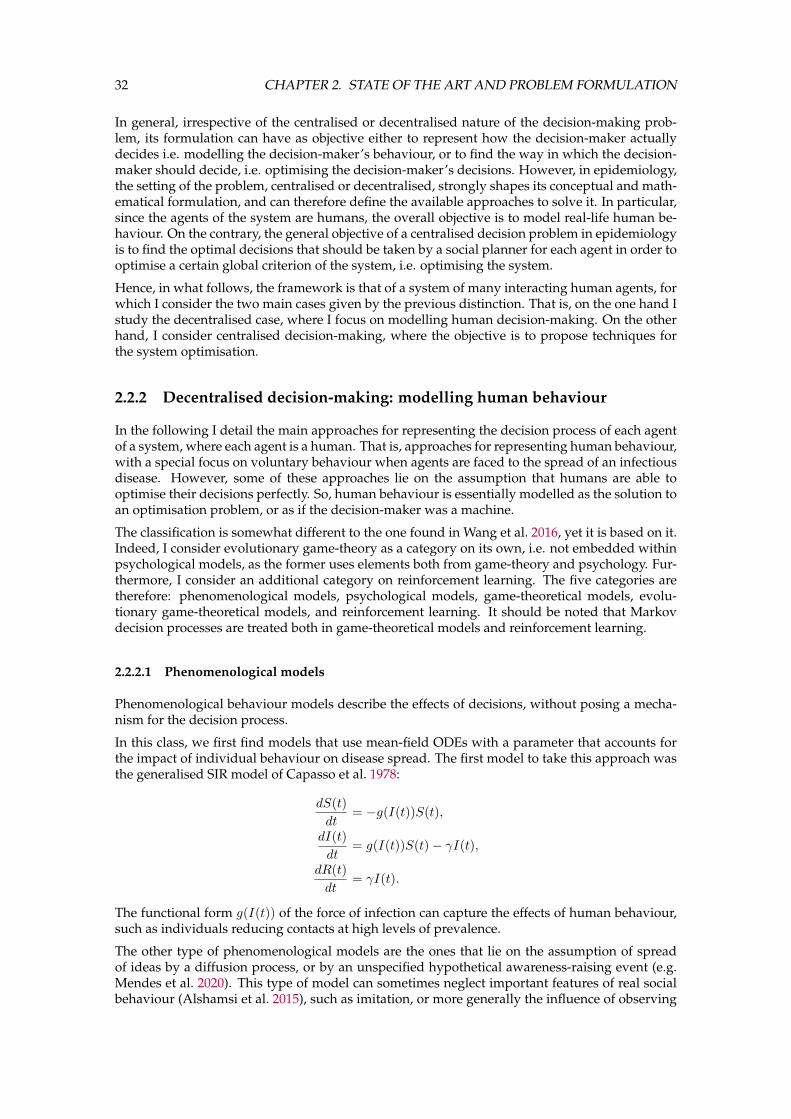
32 CHAPTER 2. STATE OF THE ART AND PROBLEM FORMULATION
In general, irrespective of the centralised or decentralised nature of the decision-making prob-lem, its formulation can have as objective either to represent how the decision-maker actuallydecides i.e. modelling the decision-maker’s behaviour, or to find the way in which the decision-maker should decide, i.e. optimising the decision-maker’s decisions. However, in epidemiology,the setting of the problem, centralised or decentralised, strongly shapes its conceptual and math-ematical formulation, and can therefore define the available approaches to solve it. In particular,since the agents of the system are humans, the overall objective is to model real-life human be-haviour. On the contrary, the general objective of a centralised decision problem in epidemiologyis to find the optimal decisions that should be taken by a social planner for each agent in order tooptimise a certain global criterion of the system, i.e. optimising the system.
Hence, in what follows, the framework is that of a system of many interacting human agents, forwhich I consider the two main cases given by the previous distinction. That is, on the one hand Istudy the decentralised case, where I focus on modelling human decision-making. On the otherhand, I consider centralised decision-making, where the objective is to propose techniques forthe system optimisation.
2.2.2 Decentralised decision-making: modelling human behaviour
In the following I detail the main approaches for representing the decision process of each agentof a system, where each agent is a human. That is, approaches for representing human behaviour,with a special focus on voluntary behaviour when agents are faced to the spread of an infectiousdisease. However, some of these approaches lie on the assumption that humans are able tooptimise their decisions perfectly. So, human behaviour is essentially modelled as the solution toan optimisation problem, or as if the decision-maker was a machine.
The classification is somewhat different to the one found in Wang et al. 2016, yet it is based on it.Indeed, I consider evolutionary game-theory as a category on its own, i.e. not embedded withinpsychological models, as the former uses elements both from game-theory and psychology. Fur-thermore, I consider an additional category on reinforcement learning. The five categories aretherefore: phenomenological models, psychological models, game-theoretical models, evolu-tionary game-theoretical models, and reinforcement learning. It should be noted that Markovdecision processes are treated both in game-theoretical models and reinforcement learning.
2.2.2.1 Phenomenological models
Phenomenological behaviour models describe the effects of decisions, without posing a mecha-nism for the decision process.
In this class, we first find models that use mean-field ODEs with a parameter that accounts forthe impact of individual behaviour on disease spread. The first model to take this approach wasthe generalised SIR model of Capasso et al. 1978:
dS(t)
dt= −g(I(t))S(t),
dI(t)
dt= g(I(t))S(t)− γI(t),
dR(t)
dt= γI(t).
The functional form g(I(t)) of the force of infection can capture the effects of human behaviour,such as individuals reducing contacts at high levels of prevalence.
The other type of phenomenological models are the ones that lie on the assumption of spreadof ideas by a diffusion process, or by an unspecified hypothetical awareness-raising event (e.g.Mendes et al. 2020). This type of model can sometimes neglect important features of real socialbehaviour (Alshamsi et al. 2015), such as imitation, or more generally the influence of observing

2.2. DECISION-MAKING WITH APPLICATION IN EPIDEMIOLOGY 33
the behaviour of other agents (Bandura et al. 1977). However, they can be useful to easily observethe effect of individuals’ behaviour on disease spread, and to describe through simple ideas howcomplex behaviours can emerge in populations (Wang et al. 2016).
A final example of a model that phenomenologically accounts for behaviour is one that dividespopulation into groups according to a static vaccination profile (such as "vaccinates" vs "does notvaccinate"), and only explores infection dynamics given the interaction of agents in the differentassigned groups (e.g. Hill et al. 2021). Indeed, such a model does not consider how the agentscan acquire (nor loose) such vaccination profiles.
2.2.2.2 Psychological models
Among the models that do formulate mechanisms to describe individuals’ behaviour we find theones that lie on specific psychological theories.
A first example are models that rely on subjective expected utility (SEU) theory (Savage 1972),which is an extension of expected utility (EU) theory. EU theory supposes that individual decisionsarise from a utility function U(xi) of the possible outcome xi of a given decision i, and theprobability of each outcome p(xi) (Machina 1987). Then, if the individual has another optionfor the decision with possible outcomes yi, it chooses the decision with the highest EU. SEUtheory adds a psychological aspect to EU theory, supposing that the agent only has a personalbelief of the probability of each outcome, and decides based on the subjective expected value ofthe utility. That is, for computing the SEU of each option, the agent uses their subjective beliefon the probabilities, and then chooses the decision with the highest SEU. It is to be stressed thatmany economic experiments have pointed out that the theory is not consistent with real humandecision-making (Karni 2008). In particular, Ellsberg 1961 used simple hypothetical experimentsto show how sometimes it can be impossible to infer probabilities from the choices made byan individual, concluding that individuals do not always decide as a function of a probabilitydistribution on the outcomes.
Another important approach is prospect theory (Kahneman et al. 1979), which belongs to be-havioural economics, a relatively recent economic field that (contrary to classical economics)accounts for psychological, cognitive, emotional, cultural and social factors on individuals de-cisions (Teitelbaum et al. 2018). Unlike EU theory, prospect theory does not consider perfectlyrational agents, i.e. agents that decide by performing a cost-benefit analysis to determine theoption that maximises their benefit at the smallest cost. In particular, it describes individualspreferring to avoid losses rather than to acquire equivalent gains. Also, it accounts for a cogni-tive human bias consisting in over-estimating the probability of very rare events. It is thereforerelevant in epidemiology for accounting for the influence of rare events, such as vaccine adverseevents or disease complications, on human decision-making (Wang et al. 2016). It has been moreoften used in mean-field models coupling vaccinating behaviour and disease spread. In partic-ular, Oraby et al. 2015 built a disease-behaviour model in the context of vaccination against apaediatric infectious disease, accounting for bounded rationality using prospect theory. In thiswork, a comparison with a simpler model where individuals behave rationally is made, show-ing that taking into account cognitive considerations in the first model could profoundly impactpredictions.
A third approach belonging to psychological models are belief-decision models. These models lieon the Dempster–Shafer theory (Shafer 2020), a general statistical framework for reasoning withuncertainty. This framework allows for an agent to combine evidence from different sources toupdate the belief on the probability of an event, belief that determines his subsequent decisions.In epidemiology, belief-decision models have been used for coupling vaccination and diseasedynamic decisions, particularly to account for the influence of awareness concerning diseaseprevalence and vaccine safety (see Xia et al. 2014).

34 CHAPTER 2. STATE OF THE ART AND PROBLEM FORMULATION
2.2.2.3 Classical game theory
Game theory studies mathematical models of strategic interactions among decision-makers (My-erson 1997). In classical game theory, individuals are generally assumed to be perfectly rational,i.e. able to perform a cost-benefit analysis to determine whether an option is good for them andto choose that option.
To be fully defined, a game must specify its players, the information and actions available to eachplayer at each decision point, and the payoffs for each outcome. Furthermore, the game can beeither cooperative, if players are supposed to be able to form alliances, or non-cooperative other-wise. Cooperative game theory focuses then on predicting coalitions, joint actions and collectivepayoffs. Meanwhile, non-cooperative game theory focuses on predicting individual players’ ac-tions and payoffs. In particular, it analyses Nash equilibria, a set of strategies for each playersuch that, when employed, no player can profit by unilaterally changing strategy.
The most studied non-cooperative game is the Prisoner’s Dilemma, formalised by Albert W.Tucker in by 1950 (Poundstone 1992). This game consists in two members of an organisation be-ing imprisoned separately without possibility for communicating with each other. Each prisonerA and B can either betray by saying that the other committed the crime. It is implicitly assumedthat prisoners cannot punish the other’s betrayal, i.e. the only thing that matters in decision is theyears of conviction they can get according to their decision. If both prisoners betray each other,each will have 2 years in prison. If one prisoner betrays, but the other remains silent, the onethat betrays will be set free and the other one will have 3 years in prison. Lastly, if both prisonersremain silent, each will have 1 year in prison.
The pay-off matrix of this game is then:
B silent B betraysA silent (-1, -1) (-3, 0)
A betrays (0, -3) (-2, - 2)
Table 2.1: The Prisoner’s Dilemma. Terms in parenthesis indicate the pay-off of the players under the givenstrategy.
From an individual point of view, betraying always results in a better payoff than keeping silentregardless of the other’s player action. Then, mutual betrayal is the only strong Nash equilibriumin the game (i.e. the only outcome from which each player could only do worse by unilaterallychanging strategy). Hence, the dilemma consists in the fact that, although mutual cooperationwould be more beneficial to both players than mutual defection, the most ‘rational’ strategy isbetraying, i.e. is the best strategy from a self-interest point of view, while keeping silent wouldbe irrational.
Classical game theory is commonly used to model human behaviour, i.e. it is commonly as-sumed that the Nash equilibria of the studied games can predict human decisions on a similarreal-life problem. This point of view regarding classical game theory has been extensively criti-cised, arguing that the assumptions made do not hold for real human decision-making processes,as humans do not always act in a fully rational way (Chang et al. 2019; Newton 2018). On theone hand, individuals can exhibit bounded rationality, given by cognitive, informational or timeconstraints that do not allow them to compute the optimal strategy, so they rather choose a sat-isfactory option (Sent 2018). On the other hand, humans can simply make irrational decisions.That is, not choose the best option from their individual point of view, for example when theyimitate others’ behaviour (Pingle 1995).
These criticisms encouraged the emergence of the field of evolutionary game theory, whichsearches to resolve these issues by avoiding to assume that individuals are perfectly rational(Wallace et al. 2015).
In epidemiology, classical game theory has been extensively used to study voluntary vaccination

2.2. DECISION-MAKING WITH APPLICATION IN EPIDEMIOLOGY 35
uptake in human populations (e.g. Bauch et al. 2004, 2003; Jijón et al. 2017; Mohr et al. 2020.In particular, the Prisoner’s Dilemma has been used for defining optimal strategies from theindividual and from the group point of view. Assuming an initial high level of vaccine coverage,vaccinators are considered to be the Cooperators, while non-vaccinators are the Defectors, whichfree-ride, i.e. benefit from the herd-immunity levels acquired by the vaccinators, without havingto bear the cost of the vaccine. At a low initial level of vaccine coverage, the Prisoner’s Dilemmais not however a relevant analogy, since what would be optimal for each individual would be toget vaccinated (Wang et al. 2016).
As mentioned before, classical game theory assumes that individuals optimise their payoffs in aselfish rational way. However, effects like social learning (i.e. learning by imitation) and boundedrationality (cognitive, informational or time constraints) are very important in vaccination deci-sions (e.g. Sturm et al. 2005). Furthermore, classical game theory mostly studies problems of onlytwo players. In a context of many interacting agents, mean field game theory (Lasry et al. 2007)studies strategic decision making in such large populations by making a mean field simplifica-tion. That is, assuming atomic agents determine their strategy by considering the evolution ofthe group of players as a whole, rather than the set of individual behaviours. Indeed, each playersearches to minimise an individual cost that depends on the agent’s state and action, and on amean criterion based on the global state of the group of players. However, the predictive valueof an approach relying on this simplification is limited for cases where disease and behaviourdynamics depend on a non-homogeneous population structure (Wang et al. 2016).
A particular game-theoretic framework that is worth mentioning here, is the one of Markovdecision processes (MDP). MDP provide a mathematical approach for modelling decision mak-ing in situations where outcomes are partly random and partly under the control of a deci-sion maker. They lie on the assumption that the conditional probability distribution of the fu-ture states of the dynamic system, given past states and the present state, only depends onthe present state and not on past states (‘absence of memory’ of a Markov process). Hence, aMDP is given by a set of states X , a set of actions A, a (Markovian) transition model Pa(x, x′) =P (xt+1 = x′|xt = x, at = a) (probability that action a in state x at time t leads to state x′ at timet + 1), and a reward function Ya(x, x′) = P (yt+1 = y|xt = x, at = a, xt+1 = x′) (probability thatyt+1, the reward at time t+ 1, equals y after transitioning from state x to state x′ due to action a).
MDP are not specific to game-theory, as they are used and studied in other fields, such as rein-forcement learning (see section 2.2.2.5). From the game-theory point-of-view, a MDP is a stochas-tic game with only one player. In epidemiology, it has been used by many authors to formulategame-theoretic models of vaccinating behaviour using mean-field and rationality assumptions(Wang et al. 2016). In particular, Reluga et al. 2011 proposes a general framework for vaccinationgames lying on three models: one CTMC for epidemiological changes at the individual scale (in-fluenced by individual’s strategy and external factors such as population state), one mean-fielddeterministic model for the infection dynamics at the population level, and one model for indi-vidual decisions. The decision model lies on a combination of classical game theory postulatesand MDP theory. Indeed, the first one assumes individuals maximise their inter-temporal ex-pected utility, since they can predict their future evolution in probabilistic terms, i.e. integrateover the probability distribution of all possible paths of their future states. Meanwhile, MDPtheory is used for the evaluation of decisions, that is, for associating values with events, andcalculating the expected value conditional on each choice.
Yet, the criticisms made to classical game-theory can also be pointed out when using MDP withinthe game-theory framework. Indeed, within this framework, the MDP lies on classical game-theoretical assumptions (i.e. individuals are fully rational), and hence the questioning regardingthe extent to which it can represent actual human decision-making still holds.
2.2.2.4 Evolutionary game theory
Here I discuss models that account for psychological or cognitive features of human behaviourbut in which decisions are based on a certain payoff. I refer to them as evolutionary game-theoretical

36 CHAPTER 2. STATE OF THE ART AND PROBLEM FORMULATION
models. Since such models are in a way inspired both by classical game theory and by psychology,they are sometimes referred to as game theoretical-psychological models.
Evolutionary game theory is the application of game theory to evolving populations in biology.It originated with the work of Maynard Smith 1982. Maynard Smith’s evolutionary version ofgame theory does not require that players are rational, only that they have a strategy. The resultsof a game show how good that strategy was, like evolution shows how good strategies are forsurviving and reproducing.
Following the works of Bauch 2005 and Fu et al. 2010, several studies subsequently used evo-lutionary game theory in human disease epidemiology to represent individual’s vaccination be-haviour in a social network (Tanimoto 2021) (e.g. Cardillo et al. 2013; Fukuda et al. 2014; Li et al.2017; Liu et al. 2012; Voinson et al. 2015). The decision of the ’vaccination game’ is usually playedbefore or after the epidemic season which allows for a ‘strategy updating’, which determines theform of the influence of the neighbours in the social network on the decisions of each individual.See figure 2.7 for an example of a two-stage vaccination game considered in evolutionary-gametheory applied to epidemiology.
Figure 2.7: Scheme of a two-stage vaccination game. At stage 1, some individuals decide to vaccinate at acost CV . At stage 2, vaccinated individuals cannot get infected (vaccine provides perfect immunity) whilenon-vaccinated individuals can get infected (and hence pay a cost of infection CI ), or remain healthy (free-ride by being indirectly protected by the vaccination of other individuals). Reproduced from Fu et al. 2010.
There are several strategy updating rules in studies of evolutionary game theory applied to epi-demiology (Tanimoto 2021). First, the Imitation Max (IM) rule, in which each player copies thestrategy of the neighbour that has obtained the largest payoff in the previous decision time. Ateach decision time step, this rule is deterministic since the individual always copies the strategyof such neighbour.
The most studied stochastic updating rule is the Fermi-Pairwise rule (individual or socially based).A pairwise rule consists in randomly selecting a neighbour and copying the neighbour’s strat-egy with a probability given by a certain function in which there is a comparison between theindividual’s payoff and the neighbour’s payoff. The Fermi-Pairwise rule uses the Fermi function(Szabó et al. 1998) which reproduces the non-linearity of human decision-making processes (Pin-gle 1995; Tanaka et al. 2021). According to this rule, the probability of an individual i switchingto the strategy of a selected neighbour j is
p(dj ← di) =1
1 + exp[−κ(Πj −Πi)], (2.8)

2.2. DECISION-MAKING WITH APPLICATION IN EPIDEMIOLOGY 37
where di is the previous strategy of i, and dj is the previous strategy of j. The parameter κ cap-tures the individual’s sensitivity to the difference on the last payoff of j and i, respectively Πjand Πi. In general, the Fermi-Pairwise rule is considered to be the strategy that most closely rep-resents individual’s vaccination behaviour, and is therefore the most used one in the literature(Tanaka et al. 2021). It has also been referred to as IB-RA (Individual Based Risk Assessment) byFu et al. 2010. An extension of this rule called SB-RA (Strategy Based Risk Assessment) has beenproposed by Kuga et al. 2019, where the probability of switching strategy depends on the com-parison between the individual’s payoff and the average payoff of neighbours with the contrarystrategy.
Most of the strategies of evolutionary game theory applied to the vaccination game imply thatthe possibility of changing strategy only appears if the comparison occurs with a neighbour orgroup of neighbours with the opposite strategy. Then, if most of the population has initiallythe same strategy (vaccinate or not vaccinate), there would be a high chance that there are nochanges when updating the individual strategies. An updating rule that does not have this issueis the Fermi-like myopic updating rule (Zhang et al. 2013). However, this rule does not considerimitation. Applied to the vaccination game, it assumes that individuals first have a perceivedpayoff of vaccinating and of not vaccinating. Then, they update their vaccination preferenceaccording to their own observation of the consequences of vaccinating or not, using a Fermifunction.
The different updating rules have been used for evaluating the effect of subsidy policies on vac-cination uptake (e.g. Kuga et al. 2019; Zhang et al. 2013). Indeed, since the cost of vaccination isusually assumed to be simply the cost of a vaccine dose, it is quite straightforward to considerthat a subsidy policy that covers such a cost could impact vaccine willingness to vaccinate. Somestudies have found that the updating rule that is considered for human decision-making canhave an impact on the efficiency of the subsidy policy (e.g. Zhang et al. 2013), or on the pathogenspread (Ning et al. 2020). In particular, Kuga et al. 2019 found that even if results are qualita-tively the same, in the case humans behave according to the IB-RA rule more individuals shouldbe subsidised when compared to the case when they behave according to the SB-RA, since in thelatter case there are more people that would vaccinate without subsidies.
The last point introduces the main limitation of this approach: a priori, it is unclear to what extentthe chosen mechanism of individual decision-making has an impact on the model’s dynamics(Tanimoto 2021) and therefore it should be carefully chosen (Wang et al. 2016). Indeed, it is oftendifficult to test on a representative sample if people actually take decisions in the way postulatedby the updating rule, in particular regarding their response to different external incentives. Whenat least small data samples can be obtained, econometrical techniques can be used to statisticallymodel individual’s decisions (e.g. Sok et al. 2020, 2018). Ultimately, these could provide a data-driven baseline to compare models issued from an evolutionary game-theoretical approach.
2.2.2.5 Reinforcement Learning
Reinforcement learning (RL), is an area of machine learning in which optimal control policies arelearned by the means of experience (by interacting through actions with a dynamic environment),as the environment’s state transition probabilities or the rewards (observations) associated witheach possible action are unknown (see figure 2.8). In the following, I review two main instances ofRL: MDP (a discrete-time stochastic control process whose basic structure is described in section2.2.2.3) and multi-armed bandit (MAB) problems.
Within RL, both MDP and MABs problems are generally concerned with a decision-maker thatis a machine, not a human. Hence, they do not usually search to represent real-life human be-haviour (i.e. how humans actually make decisions) but search the optimal sequence of actionsthat the agent should make, i.e. how the agent should make decisions in order to maximise theexpected sum of rewards. Even when social learning is considered, RL approaches are not usu-ally concerned with modelling how a group of human agents would make decisions, but withoptimising their collaboration, in particular by enabling or improving communication between
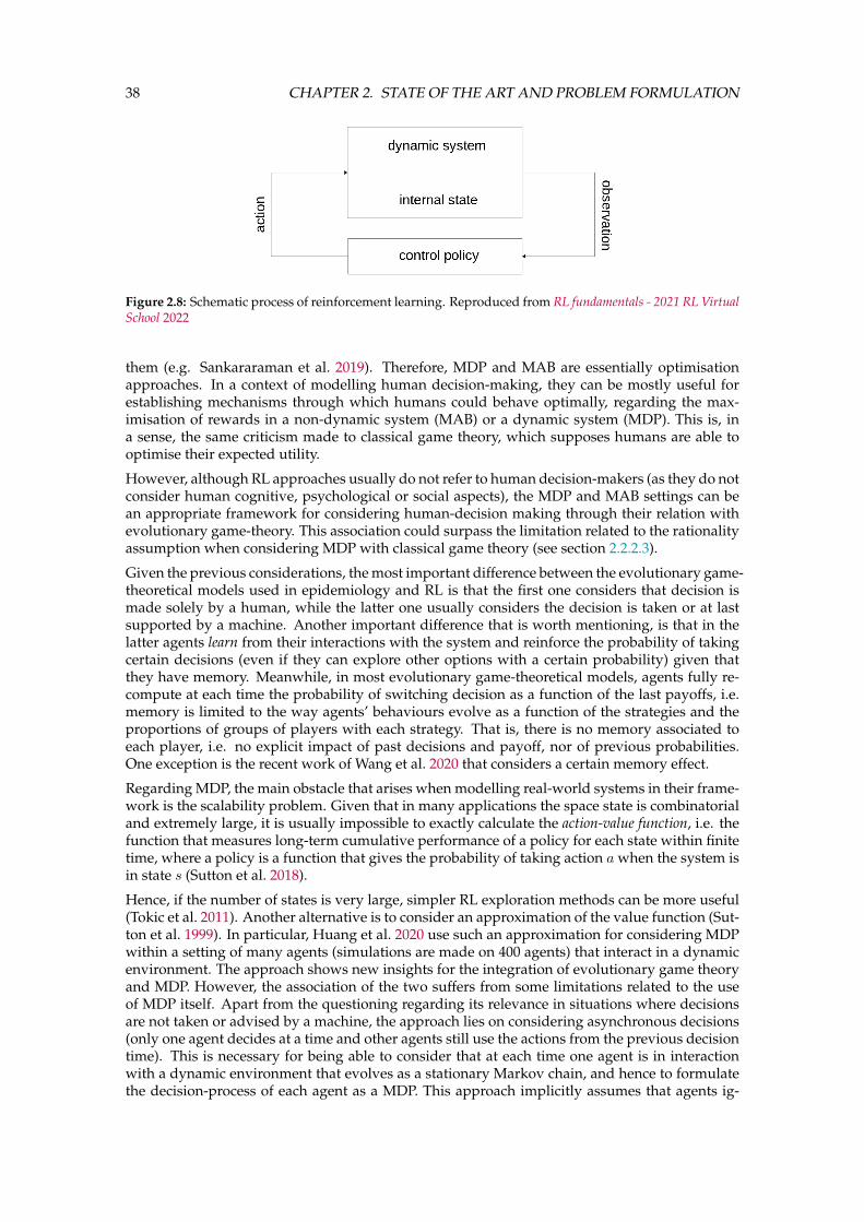
38 CHAPTER 2. STATE OF THE ART AND PROBLEM FORMULATION
Figure 2.8: Schematic process of reinforcement learning. Reproduced from RL fundamentals - 2021 RL VirtualSchool 2022
them (e.g. Sankararaman et al. 2019). Therefore, MDP and MAB are essentially optimisationapproaches. In a context of modelling human decision-making, they can be mostly useful forestablishing mechanisms through which humans could behave optimally, regarding the max-imisation of rewards in a non-dynamic system (MAB) or a dynamic system (MDP). This is, ina sense, the same criticism made to classical game theory, which supposes humans are able tooptimise their expected utility.
However, although RL approaches usually do not refer to human decision-makers (as they do notconsider human cognitive, psychological or social aspects), the MDP and MAB settings can bean appropriate framework for considering human-decision making through their relation withevolutionary game-theory. This association could surpass the limitation related to the rationalityassumption when considering MDP with classical game theory (see section 2.2.2.3).
Given the previous considerations, the most important difference between the evolutionary game-theoretical models used in epidemiology and RL is that the first one considers that decision ismade solely by a human, while the latter one usually considers the decision is taken or at lastsupported by a machine. Another important difference that is worth mentioning, is that in thelatter agents learn from their interactions with the system and reinforce the probability of takingcertain decisions (even if they can explore other options with a certain probability) given thatthey have memory. Meanwhile, in most evolutionary game-theoretical models, agents fully re-compute at each time the probability of switching decision as a function of the last payoffs, i.e.memory is limited to the way agents’ behaviours evolve as a function of the strategies and theproportions of groups of players with each strategy. That is, there is no memory associated toeach player, i.e. no explicit impact of past decisions and payoff, nor of previous probabilities.One exception is the recent work of Wang et al. 2020 that considers a certain memory effect.
Regarding MDP, the main obstacle that arises when modelling real-world systems in their frame-work is the scalability problem. Given that in many applications the space state is combinatorialand extremely large, it is usually impossible to exactly calculate the action-value function, i.e. thefunction that measures long-term cumulative performance of a policy for each state within finitetime, where a policy is a function that gives the probability of taking action a when the system isin state s (Sutton et al. 2018).
Hence, if the number of states is very large, simpler RL exploration methods can be more useful(Tokic et al. 2011). Another alternative is to consider an approximation of the value function (Sut-ton et al. 1999). In particular, Huang et al. 2020 use such an approximation for considering MDPwithin a setting of many agents (simulations are made on 400 agents) that interact in a dynamicenvironment. The approach shows new insights for the integration of evolutionary game theoryand MDP. However, the association of the two suffers from some limitations related to the useof MDP itself. Apart from the questioning regarding its relevance in situations where decisionsare not taken or advised by a machine, the approach lies on considering asynchronous decisions(only one agent decides at a time and other agents still use the actions from the previous decisiontime). This is necessary for being able to consider that at each time one agent is in interactionwith a dynamic environment that evolves as a stationary Markov chain, and hence to formulatethe decision-process of each agent as a MDP. This approach implicitly assumes that agents ig-

2.2. DECISION-MAKING WITH APPLICATION IN EPIDEMIOLOGY 39
nore each other, so the problem is reduced to a single-agent problem, and interactions with otheragents are possible only through the stochastic environment. Yet, under different conditions (inparticular synchronous decisions) the actions of all agents would have to be explicitly consid-ered in a multi-agent MDP (see section 2.2.3.3.3), and the curse of dimensionality for solvingMDP would be enhanced (Bloembergen et al. 2015).
Since there are alternative RL approaches (such as the MAB problem) that could be scalable, theycould have the potential of also addressing the concern on representing actual human-behaviour,provided that they imply less cognitive and computational resources for the decision-maker. Inparticular, if the process is not Markovian, or if the agent does not truly behaves optimally, thedecision-making process of the agent can still be formulated within the MAB setting.
Regarding MAB, they are a particular type of RL problems, much simpler than MDP. A MAB is asequential decision problem under uncertainty where an agent faces a number of options, calledarms in the MAB terminology, each with an associated distribution of rewards. Since the agentdoes not know these distributions, it chooses an arm at each decision time, in order to optimise apreviously established objective which depends on the rewards and thus on the agent’s choices(Kaufmann 2014). In general, the objective on a MAB problem is to maximise the sum of rewards(in expectation) for a given time horizon T . To do this, the agent must explore the differentoptions to obtain information on the distributions, but also exploit the options that maximise theempirical mean of the realised rewards. It will thus have to manage an exploration-exploitationtrade-off.
The most studied MAB problem is the stochastic iid problem: the reward generating process israndom, and reward observations are independent and identically distributed (i.i.d.) over time.That is, to each option corresponds an unknown distribution of rewards that is fixed in time,i.e. it is not modified either by the agent’s actions or by external elements. The generalisation ofthe stochastic MAB problem which removes all assumptions on the distribution of the arms isthe bandit adversarial problem. It supposes that at each iteration the agent chooses an arm andan ‘adversary’ simultaneously chooses the payoff structure for each arm. An example for ad-versarial bandits is the iterated prisoner’s dilemma, where two players play prisoner’s dilemmamore than once in succession and they remember previous actions of their opponent and changetheir strategy accordingly. A strategy well adapted for the adversarial bandit problem is theExp3 adversarial algorithm (algorithm 1) proposed by Auer et al. 2002b. It consists in exploitinggood arms (i.e. arms with higher weights) with probability 1 − ψ, and possibly exploring otherarms with probability ψ. After receiving the rewards, the weights are updated by exponentiallyincreasing the weight of good arms.
One can remark the similarity between the exponential weight scheme for updating probabilitiesused in the Exp3 adversarial MAB algorithm (algorithm 1), and the one in the Fermi-Pairwiserule used for computing the probability of switching decision (equation 2.8). Similarities be-tween evolutionary game theory (not restricted to its application in epidemiology) and RL (notrestricted to MAB) had been previously pointed out, mostly in the economic field (Börgers et al.1997; Vega-Redondo 2003). Their relation has however received less attention from the RL com-munity (Tuyls et al. 2005). In the field of epidemiology, Shi et al. 2019 considered RL and evo-lutionary game theory in a context of human decision-making regarding voluntary vaccination.Yet the two approaches are not actually combined together, as they refer to two different stepsof the decision-making process. Indeed, a very simple MAB algorithm is used to dynamicallydetermine if a human agent rationally decides according to the local prevalence of the disease, orif he/she imitates his/her neighbours.
More generally, evolutionary games settings can directly be formulated as MAB problems, sincemost of the heuristics in evolutionary game theory define MAB strategies that do not search to beoptimal (i.e. in which human aspects of decision-making are taken into account). Yet, as statedbefore, agents actually learn in MAB strategies, i.e. they explicitly take into account the historyof past decisions to make their following decisions, through the probabilities for the decisionoptions. Furthermore, from a methodological point-of-view, they are generally described by analgorithm that mathematically formalises all the steps of the decision-making process.

40 CHAPTER 2. STATE OF THE ART AND PROBLEM FORMULATION
Algorithm 1 Exp3 adversarial MAB algorithm (Auer et al. 2002b)
Input: ψ ∈ (0, 1], K arms.1: wk(1) = 1 for k = 1, ...,K ▷ Weights initialisation2: for t = 1, 2, ..., T do ▷ At each decision time3: pk(t) = (1− ψ) wk(t)∑K
i=1 wl(t)+ ψ
K ; k = 1, ...,K ▷ Compute the probability of pulling armk at time t as a function of the weights ofall arms and the exploration parameter ψ
4: at ←Multinom(1, (p1(t), ..., pK(t))) ▷ Draw an arm at randomly according tothe probabilities p1(t), ..., pK(t)
5: xat(t) ∈ [0, 1] ▷ Observe a reward given by the pulledarmed and the environment
6:7: for k = 1, ...,K do ▷ For each arm
8: xk(t) =
xk(t)/pk(t) if k = at
0, otherwise▷ Standardise the reward of the pulled
armed by the probability of pulling it, tocompensate for a potentially small prob-ability of getting the observed reward
9: wk(t+ 1) = wk(t)exp(ψxk(t)/K) ▷ Update the weight of the pulled arm kthrough exponential function of the ob-served standardised reward. The expo-nential growth significantly increases theweight of good arms
10: end for11: end for
2.2.3 Centralised decision-making: optimising the system
Controlling infectious diseases is a general and important problem that has been extensivelytreated in the epidemiology literature. In the following, I begin by precising the usual controllevers that are considered for infectious diseases on metapopulation networks. Then, I describesome strategies and mathematical approaches that can been used to achieve such control froma central social planner’s point of view. Even if most of the approaches have been initially andmostly applied on well-mixed populations, the focus here is on the elements that have or couldbe applied on a metapopulation network.
2.2.3.1 Control levers and practical considerations
Measures for controlling pathogen spread on metapopulation networks are generally focusedon either accelerating recovery (reducing illness duration), or decreasing the infection rate ofeach sub-population (Nowzari et al. 2015). The measures to attain the first of these two objec-tives focus on providing treatments to infected individuals, or improving existing conditions oftreatment (for example through investments in health sector facilities). Regarding the second ob-jective, there are several available measures from a centralised point-of-view, including the twoprevious ones as they can also impact the infection rate. Another measure is the distribution ofvaccines among sub-populations. Other types of measures are movement restrictions betweensub-populations (which can particularly imply quarantining some sub-populations), or acting onthe awareness of the agents regarding the disease, for example through information campaigns,to increase the adoption of control measures (self-isolation, social distancing, hygiene measures)taken at the individual level. A measure that is specific to animal health is the culling of animalsthat have been tested positive, or even culling of all animals, not necessarily in infected herds,with a more preventive objective (e.g. for herds in the neighbourhood of an infected one).
The more radical is a measure, the less likely it will be considered and adopted, especially fora disease that does not have a rapid and strong economic and health burden. For example,

2.2. DECISION-MAKING WITH APPLICATION IN EPIDEMIOLOGY 41
though movement restrictions can be very effective, as they seek to completely eliminate therisk of contagion by cutting the transmission path, they are also very costly in practice. In thecase of movement restrictions, the agricultural and societal impact should be taken into account.Furthermore, particularly in the context of animal health, the cost of culling measures is not onlyeconomical (production losses) but it also affects animal well-being.
2.2.3.2 Allocation problems
The above considerations can be formally taken into account by the means of an allocation problem,consisting in distributing a fixed budget of some sort in order to best mitigate the spread of thepathogen on the network. The constraint can be for example on the maximal number of sub-populations to isolate or immunise. The budget constraint prevents the control measure frombeing applied to the whole metapopulation, which would certainly quickly reduce the pathogenspread but is rarely applicable in real-life, mainly due to high economic costs.
The control levers described in section 2.2.3.1, can be distinguished through a main classifica-tion regarding their effect: measures that impact the network structure and measures that impactepidemiological parameters within sub-populations. Following Nowzari et al. 2015, from an op-timisation perspective, one can consider two broad problems related to the first type of measures,and a third problem regarding the second type of measures:
Problem 1 Given an original network G and a fixed budget C > 0 of nodes, minimise a functionF , by removing (isolating or immunising) at most C nodes from G.
Problem 2 Given an original network G and a fixed budget C > 0 of links, minimise a functionF , by removing at most C links from G.
Problem 3 Given a network G, given epidemiological parameters Θ, and a fixed budget C > 0 ofa resource (that has an impact on Θ), minimise a function F , by distributing the budget among theN nodes of the network, under the constraint
∑N∗
i f(i) ≤ C, where f(i) is the cost of allocatingthe resource to node i, and N∗ is the number of nodes to which the resource is actually allocated.
Usually, these problems are formalised for a static network (Cohen et al. 2003; Tong et al. 2012;Wang et al. 2003), yet they could also be considered dynamically. The first problem consists inoptimally "removing" (i.e. perfectly immunising or completely disconnecting) some nodes of thenetwork so as to prevent or reduce pathogen spread, which we refer to as node removal. Thesecond problem is link removal. This is an even more complex problem than the previous one,given that the number of links in the network can be much higher than the number of nodes.Related problems to Problems 1 and 2 can consider, instead of a complete removal, a certaintype of control, consisting for example in reducing the intensity of the contacts on the links. Thethird problem consists in optimally allocating a limited budget of a certain resource, such as atreatment or an (imperfect) vaccine, on the nodes of the network, i.e. resource allocation.
An example of an allocation problem related to the generic problem 3 is worth to be mentioned.It can be formulated as:
Problem 4 Minimise the quantity of vaccines, such that herd immunity is reached.
In problem 4, the budget to minimise is usually considered to be a quantity of vaccines thatprovide perfect and life-long immunity, and the constraint concerns reaching a herd-immunitythreshold. That is, the level at which a ’sufficient‘ percentage of the population has becomeimmune against an infection to hinder infection-related dynamics.
This problem particularly concerns the first of the approaches that are described in section 2.2.3.3.
2.2.3.3 Control approaches
In the following, I present mathematical tools that can be concerned with either of the problemsdescribed above, i.e. when the budget is expressed in the number of nodes, number of links, or

42 CHAPTER 2. STATE OF THE ART AND PROBLEM FORMULATION
in the quantity of a resource. Yet, the focus is made on the third problem, i.e. resource allocation,as the main motivation of this thesis are endemic livestock diseases, for which a strong controlof such as movement bans is not very relevant. Furthermore, the nature of the budget to allocatecan certainly determine the allocation strategy, e.g. the optimal allocation of imperfect vaccinesmay not coincide with the optimal node removal strategy. In addition, some approaches thatare feasible for determining a node removal or resource allocation strategy, could be too costly,computationally speaking, to be deployed for finding the optimal link removal strategy. Seeworks on network dismantling (Braunstein et al. 2016) or link rewiring (Schwartz et al. 2010) fora focus on approaches that are specifically adapted to node or link removal.
2.2.3.3.1 Spectral control For some of the considered problems, the function F to minimise (orthe constraint to satisfy) usually depends on the network structure (Problems 1, 2 and 4). This isusually related to reaching the herd-immunity threshold.
For classical compartmental epidemiological models, the herd-immunity threshold can be ex-pressed with respect to R0, the basic reproduction number of the infection (Keeling et al. 2011)(cf. section 2.1.1.1.1). It is possible to show that if a proportion 1− 1
R0of susceptible individuals
is perfectly immunised (the herd-immunity threshold), then the disease will be eradicated.
In a context of structured populations, much work has been devoted to determining the minimalfraction of each group that should be immunised (i.e. Problem 4), i.e. the level of vaccination foreach sub-population that minimises the spectral radius of the next-generation matrix (cf. section2.1.1.1.3), which is why such works can be grouped under the term of spectral control (Nowzariet al. 2015). These works usually consider a small number of groups, with strong interactionbetween them (e.g. Feng et al. 2017; Zhao et al. 2019). In particular, Hill et al. 2003 studiedthe properties of the solution to Problem 4, and computed the solution for an influenza A modelstratified in age groups. However, within the framework of networks, the problem of minimisingthe spectral radius by removing a given number of nodes or links are respectively NP-completeand NP-hard (Mieghem et al. 2011), so heuristics have to be used to approximate its solution.Recently, Delmas et al. 2021, combined problems 1 and 4 into a bi-objective optimisation problemon an infinite-dimensional metapopulation SIS model, studied within the framework of a kernelmodel, and proved the existence and properties of its solutions.
Spectral control approaches have also been used for solving Problem 3 by assuming it is possibleto tune the epidemiological parameters, such as the node or link dependent infection rates. Solu-tions often recur to geometric programming (Boyd et al. 2007), a type of constrained-optimisationproblem with a particular form. The first main drawback is that, since they are based solely onthe spectral radius, they do not take into account the state of the system, which can result in use-lessly allocating resources to some nodes. Additionally, although some variants of the problemcan be solved in polynomial time, this may not be sufficient for very large networks (Nowzariet al. 2015).
2.2.3.3.2 Optimal control theory Optimal control theory (OCT) is an analytical approach usedfor optimising the control of a dynamic system over a period of time (Lenhart et al. 2007). Inepidemiology, it has been widely used for finding the optimal deployment of measures such asvaccination, treatment, or quarantine, (e.g. Behncke 2000; Sethi et al. 1978). Various costs havebeen considered, in particularly integrating economic considerations (e.g. Perrings et al. 2014).
Yet, the mathematical complexity of this method limits its use to the case of dynamic systemsthat can be described by simple models. Furthermore, the strategies identified as optimal can behighly complex, for example needing for a strategy switch at specific times. This can be bene-ficial for controlling pathogen spread if the exact switch times are known, notably if there is nouncertainty in model parameters, but can lead to poor results otherwise (Bussell et al. 2019).
Complex population structures are therefore rarely considered in OCT. In particular, Mbah etal. 2011; Rowthorn et al. 2009 apply it for resource allocation in a metapopulation of only twogroups. Indeed, Zaric et al. 2001 showed that the resource allocation problem among n cou-

2.2. DECISION-MAKING WITH APPLICATION IN EPIDEMIOLOGY 43
pled sub-populations is intractable. Hence, OCT usually relies on numerical approaches to findapproximate solutions to these problems. However, such methods suffer from a lack of intuitiveinterpretation, which greatly limits their usefulness for the control of pathogen spread (Brandeauet al. 2003).
Bussell et al. 2019 proposed to overcome the limitations related to using optimal control in epi-demiology, by the means of techniques consisting in approximating the epidemiological modelby a simpler one, which facilitates the mathematical analysis necessary to OCT. A similar ap-proach by Lemaitre et al. 2021, proposes a novel OCT framework for vaccine allocation on ametapopulation network of roughly 100 nodes using a deterministic COVID-19 model. Thisframework relies on a simplification of the full model that in particular reduces the problem toa tractable size, by considering only the most important links for deriving the optimal strategy,and the full network for evaluating it. The optimal control strategy provides a benchmark for theallocation on such metapopulation, as it outperforms all the other strategies. Yet, as the optimalstrategy is complex and difficult to explain, the questioning regarding whether OCT strategieswould be adopted by decision-makers in real-life control still holds.
2.2.3.3.3 Markov decision processes RL, in particular MDP, can not only be useful for decen-tralised decision-making as discussed in section 2.2.2.5, but also refer to the decisions taken by asocial planner to control a system of many interacting agents. In this setting, the control can beformalised in two ways.
On the one hand, the social planner could take a decision for each agent of the system, in whichcase its decision process may be formulated as a centralised multi-agent MDP. On the other hand,decisions can concern the system as a whole (i.e. not be specific to each agent), in which casethe social planner is the agent whose decision process is formalised as a single-agent MDP, ashe/she should decide for the action to take at each decision time, and the interacting agents areconsidered to be part of the dynamic system (i.e. their number only increases the dimension ofthe MDP state space, not the dimension of the action space). This approach has already beenapplied in the context of livestock control by Viet et al. 2018, who proposed a MDP frameworkfor a central social planner that searches to dynamically determine the incentive to implement agiven measure, in order to optimise the collective financial benefit of a group of farmers. The in-centive impacts farmers decisions, which are taken into account in a phenomenological manner,and farmers decisions impact the costs related to the disease and control.
In both cases, the decision-maker does not explicitly consider learning processes correspondingto each agent (i.e. each agent is not a decision maker on its own), which allows to use standardMDP policy evaluation algorithms (Xuan et al. 2002). However, this implies that irrespectiveto the approach, using MDP for controlling a very large multi-agent system suffers from theclassic limitations of MDP regarding the curse of dimensionality in the system’s space state, whichis combinatorial in the number of agents. In particular Viet et al. 2018 consider a system of onlyN = 50 agents (where each agents is a herd). As each herd could either be in one of five healthcompartments, the number of states was given by
(N+44
). Additionally, from an implementation
point-of-view having such a large state space renders the optimal policy too complex to be usedin the field, which is why authors proposes an approximated policy.
2.2.3.3.4 Score-based approaches The three previous approaches formalise and address theallocation problem by searching to directly determine the optimal allocation decisions. I referhere to approaches that, instead of seeking to directly determine the order in which the resourceshould be prioritised to the nodes of a network, aim to find the optimal score to rank the nodes(and not directly the optimal decisions) for the resource allocation. Such approaches are score-based.
The scores or indicators are most often heuristics, but can alternatively be derived from a certainoptimisation procedure, i.e. optimisation-based. Furthermore, they can be dynamic or static, eitherfrom the network topology perspective, i.e. consider a dynamic or a static network, or from thepathogen spread perspective, i.e. taking or not into account the infection dynamics.

44 CHAPTER 2. STATE OF THE ART AND PROBLEM FORMULATION
For a complex network of individuals, Pastor-Satorras et al. 2002 showed that the strategy con-sisting in randomly immunising individuals does not allow to eradicate the disease. Particu-larly for scale-free networks, authors argue that their structural properties should be accountedfor. This implies to design the immunisation strategy taking into account nodes’ connectivity,which would consist in identifying and targeting the most connected individuals. This is usuallyachieved through local metrics of the network topology, i.e. centrality measures, that can be di-rectly used as heuristic scores to target the nodes. This includes classic static centrality measures(degree, PageRank, etc.) (cf. 2.1.3.1.1) and more recent temporal centrality measures, such asTempoRank (cf. section 2.1.3.2). Alternatively, the global network topology can be used to deriveoptimal scores. Examples of this are the CURE policy (Drakopoulos et al. 2014) and the maxcutminimization policy proposed by Scaman et al. 2016, where treatments are allocated according toa priority-order pre-computed offline, and the chosen priority-order is the one associated to thesolution of a minimisation problem based on the network topology.
All these topologically-based scores do not explicitly consider the dynamics of the pathogenspread, but only the potential role each node may play in the pathogen spread based on thenode’s place in the network. Yet, this is not necessarily a shortcoming of topological scores, sincedetailed information on pathogen spread is rarely available. Therefore, although scores takinginto account such information could be suited for a better control, scores that do not use updatedepidemiological information and yet perform well are eligible for disease control.
An alternative is to use strategies that rely on epidemiological information. For example, it ispossible to use data-driven or simulation-based approaches (Alamo et al. 2021). In particular,Venkatramanan et al. 2019 propose an optimisation procedure that at each decision step allocatesvaccines to the sub-population that would lead to the maximum marginal reduction in the ob-jective function according to simulations. This implies to run, at each decision step, a number ofone-step simulations that is equal to the number of sub-populations.
Otherwise, it is possible to build approximations of the objective function (the function related topathogen spread that the social planner searches to minimise, e.g. cumulative number of infectedsub-populations over time) and seek to optimise these approximations. For example Dangerfieldet al. 2019, consider the resource allocation problem in a meta-population of independent sub-populations, and approximate it as a 0-1 knapsack problem, a problem that consists in finding thesubset of items (each with a certain value and a weight) that maximise the total value of theselected items under a constraint on their total weight. Another example is the LRIE (LargestReduction in Infectious Edges) strategy for treatment allocation found in Scaman et al. 2015,where the LRIE score is derived through a greedy minimisation of a certain function associatedto the pathogen spread on an arbitrary and large network.
Finally, it can be possible to propose heuristics that are ultimately proven to correspond to op-timal, or at least locally optimal solutions of a certain objective on the pathogen spread. As anexample, the LRIE strategy was initially proposed in Scaman et al. 2014 as an heuristic consistingin targeting nodes whose recovery would minimise the number of links between infected andsusceptible nodes. Then, it was proven to be the local solution to a certain optimisation problem(Scaman et al. 2015).
2.3 Decision-making regarding the control of disease spread ona trade network: problem formulation and selectedapproaches
In order to address the methodological challenges posed by dynamic decision-making regardingthe adoption of control measures to limit the spread of a disease over a metapopulation network,and in the light of the state of the art presented in this chapter, I made the following modellingand formalism choices.
First, regarding the modelling framework, the motivation of the work (unregulated livestock dis-

2.3. PROBLEM FORMULATION AND SELECTED APPROACHES 45
eases spreading on an animal trade network) strongly suggests the use of a metapopulation net-work. Also, the internal sub-population infection dynamics and demographic changes are im-portant features to be taken into account. Oversimplifying this internal dynamics could result ina loss of important characteristics of the system that emerge from this complexity. Furthermore,regarding the type of measures to consider, I decided to focus on within sub-population healthmanagement such as vaccination, instead of more stringent measures (such as trade movementrestrictions). Indeed, for unregulated diseases and from a decentralised point-of-view it seemedunlikely that farmers would impose such strong restrictions on themselves. In addition, de-cisions involving measures that alter the network are more difficult to consider, especially inoptimisation from a centralised perspective.
Second, concerning the decentralised decision approach, the choice was driven by the considerationsin table 2.2, which summarises the main advantages and limitations of each approach presentedin the state of the art. The following remarks were accounted for in the studies presented in chap-ters 3 and 5. Here, the main considered factor was the extent to which the approach could repre-sent real-life human behaviour. Therefore, I chose not to consider phenomenological approachesas they could not show how behaviours emerge in the population. Also, even if classical game-theory studies strategic interactions among agents, the rationality assumption seemed a stronglimitation in the representation of actual human behaviour under uncertainty. This issue is over-come by psychological models, yet these generally do not explicitly account for phenomena thatcan be important in the emergence of human behaviours, such as imitation dynamics. Finally,although a complex reinforcement learning approach (using Markov decision processes) couldhave been used, it offered little to account for real-life considerations, particularly for cognitiveconstraints in the farmers’ decision-process.
Approach Advantages LimitationsPhenomenological Simple way of accounting for human
behaviourDirectly assumes an effect that couldbe caused by a decision, not thedecision-making process. Hence, it isunclear whether the effect can actuallyemerge from the behaviour.
Classicalgame-theory
Rigorous mathematical frameworkunder rationality assumption
Does not account for humans havinglimited rationality (either for cognitiveor psychological reasons, or becausethey imitate each other).
Psychological Accounts for individuals’ limited ra-tionality for cognitive and psychologi-cal reasons.
In general, does not consider limitedrationality that can arise in a system ofmany interacting agents, for examplethrough imitation.
Evolutionarygame-theory
Can account for stochastic behaviourand human decision-making, as itmakes no assumptions on the individ-ual’s rationality.
In general, individuals are not as-sumed to actually learn, as the prob-ability of switching decision is notupdated based on previous decisiontimes, but only as a function of thenew payoffs.
ReinforcementLearning
Can account for stochastic behaviour,learning (reinforcing good choicesover time), and exploring. Algorith-mic formalisation flexible enough forgeneric dynamic decision problems.
The decision-maker is essentially amachine, i.e. not intended to repre-sent voluntary human behaviour, butto optimally solve a sequential deci-sion problem by learning. Hence, al-gorithms do not usually consider hu-man cognitive, psychological, and so-cial aspects.
Table 2.2: Summary of the main advantages and limitations of decentralised decision-making approachesfor modelling human-behaviour regarding voluntary control of an infectious disease.
There are similarities between the other two approaches, evolutionary game-theory and rein-

46 CHAPTER 2. STATE OF THE ART AND PROBLEM FORMULATION
forcement learning, in particular between the Exp3 MAB adversarial algorithm of Auer et al.2002b (algorithm 1) and the most used rule-of-thumb of evolutionary game-theory in epidemi-ology, the Fermi-Pairwise rule (equation 2.8). Both approaches, MAB and evolutionary game-theory, have limitations regarding their suitability to the context presented in this thesis. Indeed,on the one hand, the simple heuristics of evolutionary game-theory in epidemiology are basedon cognitive considerations for representing human decision-making. Yet, such heuristics donot usually consider that the decision-makers learn, and are not formalised as algorithms, whichlimits their generalisation. On the other hand, MAB algorithms are not really intended to rep-resent human decision-making. Yet, they seem appropriate for formalising a decision-makingmechanism, since they explicitly consider a learning process.
For the above reasons, the two approaches (evolutionary game-theory and reinforcement learn-ing) seemed the most suitable way of addressing the challenges regarding decentralised decision-making, particularly through the use of adapted multi-armed bandit algorithms inspired by theheuristics of evolutionary game theory.
Third, regarding the centralised decision approach, i.e. the optimisation of the system made by asocial planner, the choice of the method was made by integrating the considerations in table 2.3that summarises the reviewed approaches concerning allocation problems. These considerationsunderlie the work presented in chapter 4.
Approach Advantages LimitationsSpectral control Directly addresses the topology of
the population networkDoes not consider the system state.Intractable for very high dimen-sions.
Optimal control theory Can take into account the systemstate. Theoretical guarantees on thetrue optimal strategy.
Intractable for very high dimen-sions. When approximation-basedapproaches are used to address di-mensionality, no intuitive interpre-tation of the optimal strategy.
MDP Can take into account the systemstate. Theoretical guarantees onthe true optimal strategy. Usefulin the absence of a mathematicalmodel of the dynamic system, whenused with a RL perspective (learnthrough experience).
Intractable for very high dimen-sions. When approximation-basedapproaches are used to address di-mensionality, no intuitive interpre-tation of the optimal strategy.
Score-based Some can take into account the sys-tem state. Approaches can be scal-able and strategies have an intuitiveinterpretation.
No guarantee on achieving a globaloptimum, i.e. may not solve the al-location problem in an optimal way.
Table 2.3: Summary of the main advantages and limitations of centralised decision-making approaches foroptimising the control of an infectious disease on a network-structured system.
Here, the main factor that motivated the choice was the scalability of the approach. Indeed, themotivation of this work concerns very large networks of animal populations. Approaches en-sued from spectral control did not appear as computationally feasible for explicitly taking intoaccount the structure of very large networks. Furthermore, they did not allow to integrate thesystem’s epidemiological state. Optimal control theory and MDP approaches seemed in theoryparticularly well-suited for controlling the system by determining the sequence of allocation de-cisions that would optimise a global objective. However, they could not be used for such a largeproblem without resorting to approximations that no longer have guarantees of optimality andthat neglect the network structure or the intra-node dynamics. Furthermore, while using suchapproximations allows for dealing with relatively large networks, the policies have no intuitiveinterpretation and seem therefore not suitable for providing advice to real-life decision-makerson how to allocate the available resource.
Hence, the choice concerning centralised decision-making fell on score-based approaches. Al-

2.3. PROBLEM FORMULATION AND SELECTED APPROACHES 47
though those methods do not necessarily have optimality guarantees, they are scalable and canallow an intuitive interpretation of the allocation policies, which could motivate their adoptionby a central social planner.


Chapter 3
Accounting for farmers’ controldecisions in a model of pathogenspread through animal tradeCristancho Fajardo, L., Ezanno, P., and Vergu, E. (2021). “Accounting forfarmers’ control decisions in a model of pathogen spread through animaltrade”. In: Scientific Reports 11. DOI: 10.1038/s41598-021-88471-6
Contents3.1 Introduction . . . . . . . . . . . . . . . . . . . . . . . . . . . . . . . . . . . . . . . 503.2 Integrative model . . . . . . . . . . . . . . . . . . . . . . . . . . . . . . . . . . . . 51
3.2.1 Epidemic model with demography in a metapopulation based on a tradenetwork . . . . . . . . . . . . . . . . . . . . . . . . . . . . . . . . . . . . . 51
3.2.2 Farmers’ decision-making model . . . . . . . . . . . . . . . . . . . . . . . 543.2.3 An epidemic control measure . . . . . . . . . . . . . . . . . . . . . . . . . 563.2.4 An economic-epidemiological cost function . . . . . . . . . . . . . . . . . 57
3.3 Setting for simulations and sensitivity analyses . . . . . . . . . . . . . . . . . . 583.3.1 Fixed simulation setting . . . . . . . . . . . . . . . . . . . . . . . . . . . . 583.3.2 Parameters of the integrative model . . . . . . . . . . . . . . . . . . . . . . 643.3.3 Sensitivity analysis experiments . . . . . . . . . . . . . . . . . . . . . . . . 64
3.4 Results of the simulation study and sensitivity analyses . . . . . . . . . . . . . 663.4.1 Model predictions for different decision scenarios . . . . . . . . . . . . . . 663.4.2 Key determinant parameters of decision-making and epidemiological dy-
namics . . . . . . . . . . . . . . . . . . . . . . . . . . . . . . . . . . . . . . 743.5 Discussion . . . . . . . . . . . . . . . . . . . . . . . . . . . . . . . . . . . . . . . . 76
Accounting for individual decisions in mechanistic epidemiological models remains a challenge,especially for unregulated endemic animal diseases for which control is not compulsory (section3.1). We propose an original integrative model built by combining two sub-models. The first onecorresponds to the dynamics of a livestock epidemic on a metapopulation network, groundedon demographic and animal trade data (section 3.2.1). The second one describes farmers’ be-haviour regarding the adoption of a control measure against the disease spread in their herd, i.e.decentralised decision-making (section 3.2.2). The measure is specified as a protective vaccine(section 3.2.3) with given economic implications (section 3.2.4), and the model is numericallystudied through intensive simulations and sensitivity analyses (sections 3.3 and 3.4). This studyis relevant for the understanding of the interplay between decision related human behaviour and
49

50 CHAPTER 3. ACCOUNTING FOR FARMERS’ DECISIONS
livestock epidemic dynamics (detailed discussion in section 3.5). The model can be used for otherstructures of epidemic models or different interventions, by adapting its components.
The modelling choices in this chapter were motivated by the state of the art in section 2.1.1.1.2,section 2.1.1.1.4 and section 2.1.3.4, regarding epidemiological modelling, and in section 2.2.2 andsection 2.3, regarding decentralised decision-making modelling.
3.1 Introduction
Fighting livestock diseases spreading through animal trade is a major issue to guarantee sustain-able farming, competitive agrifood chains and public health (Tomley et al. 2009). Epidemic pre-vention and reduction of prevalence require improved methods of control and compliance of theactors, especially for non-regulated diseases for which control decisions are left to individual orcollective initiatives (Carslake et al. 2011). Mechanistic epidemiological models can provide a re-fined mathematical description and understanding of the complex system involved in pathogenspread, and be used to assess the effectiveness of control measures. They are complementary toobservational or experimental approaches (Keeling et al. 2011). However, accounting for humanbehaviour in such models in order to increase their predictive power remains a challenge (Hi-dano et al. 2018; Manfredi et al. 2013), in particular for livestock diseases spreading through atrade network.
Indeed, most works on infectious diseases that consider the adoption of control measures usuallydo not account for human decision-making (Wang et al. 2016) or they do not consider a structuredpopulation (Morin et al. 2013; Perrings et al. 2014). In particular, in models based on a metapopu-lation over an explicit network (Keeling et al. 2005) such as Colizza et al. 2008a, control decisionsare usually assumed to be taken at a centralised level (e.g. Braunstein et al. 2016; Scaman et al.2016). Furthermore, when human decision-making is explicitly taken into account, it generallyfocuses on the context of human diseases (e.g. Fu et al. 2010; Kuga et al. 2019; Wang et al. 2012),but it has barely been applied to veterinary epidemiology yet (Horan et al. 2010). However, inthe context of animal diseases, the decision of implementing control measures can be much moreinfluenced by economic considerations than for human diseases, an aspect that should be takeninto account in the decision model. Finally, in the field of veterinary epidemiology, studies havebeen mostly focused on regulated diseases, so human behaviour mainly consists in delaying theapplication of a central policy (e.g. Tago et al. 2016). In the few works that investigate controlmeasures for unregulated animal diseases, there is generally no dynamic feedback on decisiondue to epidemic evolution (Rat-Aspert et al. 2010). Additionally, some real-life aspects, suchas farmers having limited rationality or learning are generally missing (Krebs et al. 2018; Shi etal. 2019). There is therefore a special need for models combining the dynamics of an epidemicprocess that takes place on a livestock trade network, and the behaviour of farmers regardingthe voluntary implementation of control measures (Brooks-Pollock et al. 2015; Heesterbeek et al.2015).
We build an integrative model that can meet this need by coupling the dynamic spread of alivestock disease over a structured metapopulation, and the dynamics of the human decision-making process for applying a sanitary measure against the epidemic spread. To model theepidemic spread through a trade network we use a stochastic compartmental model that takesinto account demographic dynamics and animal exchanges. The population structure of themodel is calibrated using real data. Our decision model is inspired by previous studies (Fuet al. 2010; Kuga et al. 2019; Wang et al. 2012), in which the result of a decision regarding thevoluntary adoption of a control measure for a human disease is evaluated after being applied,and preferences over the possible decisions are updated through time. We specifically formalisethe dynamic decision problem that each farmer faces, and propose a mechanism that representsfarmers’ decision-making process in such a context. Our formalisation considers some real-lifephenomena that can be present in the context of human decision-making: stochastic behaviour,learning, and the emergence of imitation and free-riding (Hershey et al. 1994).

3.2. INTEGRATIVE MODEL 51
First, we present the two components of the integrative model: the epidemic-demographic model,and the decision model. Then, we describe the specific control measure we consider, as well asits economic implications. Later, we describe the setting for simulations and sensitivity analyseswe perform on the model, as well as the results of this simulation studies. Finally, we examinethe model as well as the results of numerical explorations.
3.2 Integrative model
In the following, we describe the two main components of our integrative model: the epidemic-demographic one, and the decision-making one. We then detail the integrative model by consid-ering vaccination as a specific control measure.
3.2.1 Epidemic model with demography in a metapopulation based on a tradenetwork
For this work we place ourselves in the context of a hypothetical livestock infectious diseasethat is transmitted only through a contact network structure consisting in herds that exchangeanimals. This population structure is inspired by real data on animal movements, extracted fromthe French Cattle Identification Database (FCID). We assume this is a closed metapopulation, thatis, we neglect exchanges with herds outside of it. This livestock trade network can be describedas a directed weighted time-varying network, where nodes represent herds and links representanimal trade. The direction of each link is determined by the transfer’s direction, and its weightcorresponds to the amount of animals exchanged. By nature, this network is time-varying sincelinks may change over time. In fact, not only trade connections may appear or disappear, but theamount of animals exchanged can vary on a daily basis.
Given this trade network, we consider an infectious livestock disease that can potentially bespread on it, and that can only be directly transmitted between animals within the same herd.The disease is assumed to be spread between herds only by animal transfers, as can be observedfor diseases such as paratuberculosis (Beaunée et al. 2015), bovine tuberculosis when there is nocontact with wildlife (Cousins 2001), and porcine reproductive and respiratory syndrome virus(Mortensen et al. 2002). In addition, the infection risk and status are assumed independent ofanimal breed, age or sex. In the absence of any intervention, the intra-herd disease spread is de-scribed by a stochastic SIR model (Keeling et al. 2011) with demography, accounting for animaltransfers over the trade network. In a compartmental SIR model, the population is divided intothree compartments: Susceptible (S), Infected (I), and Recovered (R), according to their healthstatus. The only two possible transitions in a basic SIR model correspond to infection (S→I) andrecovery (I→R). The implicit modelling assumptions we make are the following: intra-herd ho-mogeneous mixing, meaning that the contact rate is the same among all the animals in a givenherd; absence of a latent period, i.e. animals become infectious as soon as they are infected; acqui-sition of immunity after recovery; no vertical transmission, i.e. no mother-to-child transmissionduring pregnancy or childbirth; frequency-dependent intra-herd transmission, i.e. the transmis-sion rate depends on the proportion of infected animals in the herd, rather that on their number;variation in time of herd size due to births, deaths and animal transfers, which we assume arenot affected by the disease prevalence. The intra-herd transmission of the disease (without anyintervention) can therefore be described by the scheme in figure 3.1.

52 CHAPTER 3. ACCOUNTING FOR FARMERS’ DECISIONS
µ jN j(t)+∑i θi jSi(t) ∑i θi jIi(t) ∑i θi jRi(t)
S j I j R j
[τ j +∑i θ ji]S j(t) [τ j +∑i θ ji]I j(t) [τ j +∑i θ ji]R j(t)
β jI j(t)N j(t)
S j(t) γI j(t)
Figure 3: Kalman filter system model
µ jN j(t)+∑i θi jSNVi(t) ∑i θi jIi(t) ∑i θi jRi(t)
[τ j +∑i θ ji]SNVj(t) SNVj I j R j
∑i θi jSVi(t) SVj
[τ j +∑i θ ji]SVj(t) [τ j +∑i θ ji]I j(t) [τ j +∑i θ ji]R j(t)
β jI j(t)N j(t)
S j(t)
β vj
I j(t)N j(t)
S j(t)
γI j(t)
Figure 4: Kalman filter system model
2
Figure 1. Schematic representation of the intra-herd epidemic-demographic dynamics for a herd j, without any control measure.Horizontal arrows represent transitions between health-related compartments, corresponding to the course of infection inside the herd (yellowrectangle), while vertical arrows represent population flows to and from the herd. The coefficients on the arrows are the transition rates. Seemain text in Methods for parameter definitions.
evaluating the effect of the time length between successive decisions on the behavior of the integrative model. Formally, we90
suppose that each farmer j = 1, ...,J searches to solve:91
minat
j
E[Ct
atj( j)]
; t = ∆d ,2∆d ,3∆d ... (1)
where t = ∆d ,2∆d ,3∆d ... are the decision times, so ∆d is the duration (in days) between any two consecutive decisions. It also92
determines the instant at which the first decisions are taken. The term atj ∈ 0,1 refers to the control decision: if at
j = 1,93
the control-measure is applied in herd j at decision time t, otherwise it is not. Ctat
j( j) is the cost in herd j associated with the94
decision taken at time t. This constitutes a dynamic decision-making problem under uncertainty, this latter affecting the cost95
distribution associated with each possible decision.96
To define the farmer’s decision-making process that attempts to solve this problem, we take an approach inspired by [13–15],97
in which farmers evaluate the result of a decision after its application, and update their preferences over time as a function of98
this result. In this particular context, this approach seems suitable for several reasons. First, as we mentioned earlier, costs over99
time not only depend on the epidemic and decision dynamics in the herd where the decision is made, but also on other herds.100
To exactly solve this optimization problem would imply that farmers integrate the actions and epidemic status of other herds.101
This is a very complex problem due to the dimensionality on the number of herds, and on the possible status of the system.102
Second, since we pose a dynamic decision-making problem, there is an effect of learning through repeated decisions. Indeed,103
we have supposed that the cost associated to a decision is observed before making the next decision. Then, it is natural to think104
that farmers learn from the costs they have obtained with their previous choices, to take their next decisions. Finally, through105
this approach we can easily consider social dynamics such as imitation effects between farmers. In our context, this consists in106
considering a stochastic decision mechanism where the probability of applying the measure is updated through the costs each107
farmer observes over time, and the costs observed by his/her neighbors.108
The mechanism we propose (Algorithm 1) works by updating the probability of applying the measure, proportionally to an109
exponential weight that takes into account the last decision taken by the farmer and that taken by one of his/her neighbors,110
through a weighted sum of the associated costs. Then at each decision time, each farmer j = 1, ...,J takes a decision atj using111
his/her current probability of applying the measure pt1( j). We assume that this probability is initially the same for all farmers,112
and equal to a value pinit1 , and that each farmer observes the cost related to his/her decision, and the decision and associated cost113
observed by one of his/her neighbors in the trade network, who is randomly chosen by the farmer. A neighbor of j in the trade114
network is a farmer with whom j exchanges animals according to the daily trade rates, i.e. a farmer j∗ such that θ j j∗ 6= 0, or115
θ j∗ j 6= 0. In the algorithm, we note as B( j) the set of neighbors of j in the trade network.116
The update in the probability is then given by Equation 2. The parameter κ represents farmer’s “sensitivity” to his/her own117
observed costs. A κ close to zero implies that farmers are not very sensitive to their own observed costs, and therefore mostly118
rely on their initial probability of applying the measure, whereas a large κ represents the situation in which farmers are very119
sensitive to their own observed costs for updating their probability of applying the measure. For considering an imitation effect,120
we introduce the parameter ρ that works analogously to κ , but on the cost observed by the chosen neighbor. The parameters κ121
and ρ act then as weights to the farmer’s and the neighbor’s observed cost, respectively. In our model, farmer’s next decision122
can be updated considering any of his/her neighbors, regardless of what the neighbor has decided in the previous step. Finally,123
for updating the probabilities, it is natural that these are set so that the decision with a smaller sum of weighted costs receives124
higher probability. Although there are many ways to turn the sum of weighted costs into probabilities, a simple and popular125
method is to use an exponential weighting scheme. This scheme quickly reduces the probability of the decision that has resulted126
3/16
Figure 3.1: Schematic representation of the intra-herd epidemic-demographic dynamics for a herd j, with-out any control measure. Horizontal arrows represent transitions between health-related compartments,corresponding to the course of infection inside the herd (yellow rectangle), while vertical arrows representpopulation flows to and from the herd. The coefficients on the arrows are the transition rates.
Formally, we consider J herds in the population. Without any control-related measure, for eachherd j = 1, ..., J the intra-herd transmission of the disease between times t ≥ 0 and t+ δt whereδt > 0, is described by a stochastic SIR model with demography, characterised by the followingupdating equations:
Sj(t+ δt) = S∗j (t) +BSj(t) +←−Sj(t), (3.1)
Ij(t+ δt) = I∗j (t) +NSj→Ij (t) +←−Ij (t), (3.2)
Rj(t+ δt) = R∗j (t) +NIj→Rj(t) +
←−Rj(t), (3.3)
where Sj(t), Ij(t), Rj(t) are the number of susceptible, infected and recovered animals in herd jfor t ≥ 0. We suppose Sj(0) > 0 for all j, Ij(0) > 0 for at least one herd j, Rj(0) = 0 for all j. Wenote as Nj(t) = Sj(t) + Ij(t) + Rj(t) the size of herd j at time t. The terms NXj→Yj
(t) representthe number of animals going from epidemic state X to Y in herd j in the time interval ]t, t+ δt].BSj(t) is the number of births.
←−Sj(t),
←−Ij (t),
←−Rj(t), are the number of susceptible, infected and
recovered animals (respectively) purchased by herd j. Finally, S∗j (t), I∗j (t), R
∗j (t) are the number
of susceptible, infected and recovered at time t that remain in the same state after all outgoingflows are accounted for. Each one of the terms results from a stochastic process. In order toprecise the probabilities of the different possible change events in the status of an animal, we firstdefine the following epidemic and demographic daily rates:
• βj : daily rate of transmission of the disease in herd j. That is, the rate at which a susceptibleanimal gets infected by contact with an infected one in herd j. It is equal to the productbetween the contact rate in the herd, and the transmission rate of the disease if there iscontact. Then, the rate at which a susceptible becomes infected by contact with the Ij(t)infected is βj
Ij(t)Nj(t)
.
• γ: self-recovery rate of the disease. That is, the rate at which the infected individuals re-cover from the disease. Equivalent to the inverse of the mean duration (in days) of theinfectious period.
• τj : daily crude death rate in herd j. That is, the rate at which the animals are removed fromherd j (not related to the disease).
• µj : daily crude birth rate in herd j. It is the rate at which new animals are born in a herd.
•−→θj : daily out rate from herd j. It corresponds to
∑i=j θji where θji is the daily out rate from
herd j to herd i, that is, the mean number of animals going from herd j to herd i in a day,over the mean population of herd j in a day.

3.2. INTEGRATIVE MODEL 53
The stochasticity is considered in continuous time, but simulated in discrete time. The simulationin discrete time appears as more natural given available data, and is computationally more effi-cient. Formally, we consider a continuous time Markov chain simulated by an Euler simulationscheme that uses coupled discrete-time multinomial processes, as described in Bretó et al. 2009.In order to increase computational efficiency, we adapt this scheme by splitting it into two steps:one for the intra-herd epidemic-demographic dynamics, and one for the inter-herd dynamics.
In the first step, we use the coupled Multinomial chains defined by:
NSj→Ij(t), NSj→Dj
(t),−→Sj(t), S
∗j (t)←Multin
(Sj(t),
[pSIj
, pSDj, p−→
Sj, 1−
(pSIj
+ pSDj+ p−→
Sj
)]), (3.4)
NIj→Rj(t), NIj→Dj
(t),−→Ij (t), I
∗j (t)←Multin
(Ij(t),
[pIRj
, pIDj, p−→
Ij, 1−
(pIRj
+ pIDj+ p−→
Ij
)]), (3.5)
NRj→Dj(t),−→Rj(t), R
∗j (t)←Multin
(Rj(t),
[pRDj
, p−→Rj, 1−
(pRDj
+ p−→Rj
)]), (3.6)
BSj(t)← Bin(Nj(t), pBj
), (3.7)
where NSj→Dj (t), NIj→Dj (t), NRj→Dj (t) are the number of deaths of susceptible, infected, andrecovered individuals, respectively.
−→Sj(t),
−→Ij (t),
−→Rj(t) are the number of susceptible, infected
and recovered animals (respectively) sold in the same period by herd j. Each term pXYjrefers
to the probability of an animal in herd j of going from epidemiological compartment X to thecompartment Y , and p−→
Xjrefers to the probability that an animal of compartmentX is sold. These
probabilities are defined as:
pSIj=
1− e−(βj
Ij(t)
Nj(t)+τj+
−→θj
)δt
βjIj(t)
Nj(t)
βjIj(t)
Nj(t)+ τj +
−→θj
, pSDj=
1− e−(βj
Ij(t)
Nj(t)+τj+
−→θj
)δt
τj
βjIj(t)
Nj(t)+ τj +
−→θj
, (3.8)
p−→Sj
=
1− e−(βj
Ij(t)
Nj(t)+τj+
−→θj
)δt
−→θjβj
Ij(t)
Nj(t)+ τj +
−→θj
,
pIRj=
(1− e−
(γ+τj+
−→θj
)δt
)γ
γ + τj +−→θj
, pIDj=
(1− e−
(γ+τj+
−→θj
)δt
)τj
γ + τj +−→θj
, p−→Ij
=
(1− e−
(γ+τj+
−→θj
)δt
)−→θj
γ + τj +−→θj
, (3.9)
pRDj=
(1− e−
(τj+−→θj
)δt
)τj
τj +−→θj
, p−→Rj
=
(1− e−
(τj+−→θj
)δt
)−→θj
τj +−→θj
, (3.10)
pBj= 1− e−µjδt . (3.11)
In the second step, we randomly assign a destination to each exiting animal of the herd j = 1, ..., J .LetCh(j) = i = 1, ..., J : θji = 0, and let j∗1 , ..., j∗|Ch(j)| be the elements of that set, where |Ch(j)|is its cardinality. That is, the herds for which herd j is a seller according to θji; i = 1, ..., J . Wedefine Sjj∗(t), Ijj∗(t), Rjj∗(t) as the number of susceptible, infected and recovered animals, re-spectively, sold by herd j to herd j∗ in ]t, t + δt]. So that
−→Sj(t) :=
∑j∗∈Ch(j) Sjj∗(t),
−→Ij (t) :=
∑j∗∈Ch(j) Ijj∗(t),
−→Rj(t) :=
∑j∗∈Ch(j)Rjj∗(t). Then, the assignation of destination for sold ani-
mals of herds j = 1, ..., J is obtained through the following coupled multinomial chains:
Sjj∗1(t), ..., Sjj∗|Ch(j)|
(t)←Multin
−→Sj(t),
−→p jj∗1, ...,−→p jj∗|Ch(j)|−1
, 1−∑
j∗=j∗1 ,...,j∗|Ch(j)|−1
−→p jj∗
, (3.12)
Ijj∗1(t), ..., Ijj∗|Ch(j)|
(t)←Multin
−→Ij (t),−→p jj∗1
, ...,−→p jj∗|Ch(j)|−1, 1−
∑j∗=j∗1 ,...,j∗|Ch(j)|−1
−→p jj∗
, (3.13)
Rjj∗1(t), ..., Rjj∗|Ch(j)|
(t)←Multin
−→Rj(t),
−→p jj∗1, ...,−→p jj∗|Ch(j)|−1
, 1−∑
j∗=j∗1 ,...,j∗|Ch(j)|−1
−→p jj∗
, (3.14)

54 CHAPTER 3. ACCOUNTING FOR FARMERS’ DECISIONS
where the probabilities −→p jj∗ ; j∗ = j∗1 , ..., j∗|Ch(j)| are defined according to the rates θjj∗ analo-
gously to the previous multinomial chains:
−→p jj∗ =
(1− e−δt
∑j∗∈Ch(j) θjj∗
)θjj∗
∑j∗∈Ch(j) θjj∗
. (3.15)
Finally, the terms referring to the entries in herd j are computed as:←−Sj(t), :=
∑i =j Sij(t),
←−Ij (t) :=∑
i =j Iij(t), and←−Rj(t) :=
∑i=j Rij(t).
3.2.2 Farmers’ decision-making model
We suppose that farmers can apply a sanitary measure that has a certain efficacy on the diseasespread for a limited amount of time. Then, we assume they search to take the control decisionthat allows them to obtain an optimal value of an individual criterion, i.e. an expected costresulting from the decision. To consider a simple and clear framework, we restrict ourselves tobinary decisions (the measure is applied or not). Additionally, we make the assumption thatdecision times are synchronized, discrete, and equally spaced in time. This proves to be usefulwhen considering the interaction of farmers’ decisions, and for evaluating the effect of the timelength between successive decisions on the behaviour of the integrative model. Formally, wesuppose that each farmer j = 1, ..., J searches to solve:
minatj
E[Ctatj
(j)]
; t = ∆d, 2∆d, 3∆d..., (3.16)
where t = ∆d, 2∆d, 3∆d... are the decision times, so ∆d is the duration (in days) between anytwo consecutive decisions. It also determines the instant at which the first decisions are taken.The term atj ∈ 0, 1 refers to the control decision: if atj = 1, the control-measure is appliedin herd j at decision time t, otherwise it is not. Ctatj (j) is the cost in herd j associated with thedecision taken at time t. This constitutes a dynamic decision-making problem under uncertainty,this latter affecting the cost distribution associated with each possible decision.
To define the farmer’s decision-making process that attempts to solve this problem, we take anapproach inspired by Fu et al. 2010; Kuga et al. 2019; Wang et al. 2012, in which farmers evaluatethe result of a decision after its application, and update their preferences over time as a functionof this result. In this particular context, this approach seems suitable for several reasons. First, aswe mentioned earlier, costs over time not only depend on the epidemic and decision dynamics inthe herd where the decision is made, but also on other herds. To exactly solve this optimizationproblem would imply that farmers integrate the actions and epidemic status of other herds. Thisis a very complex problem due to the dimensionality on the number of herds, and on the possiblestatus of the system. Second, since we pose a dynamic decision-making problem, there is an effectof learning through repeated decisions. Indeed, we have supposed that the cost associated to adecision is observed before making the next decision. Then, it is natural to think that farmerslearn from the costs they have obtained with their previous choices, to take their next decisions.Finally, through this approach we can easily consider social dynamics such as imitation effectsbetween farmers. In our context, this consists in considering a stochastic decision mechanismwhere the probability of applying the measure is updated through the costs each farmer observesover time, and the costs observed by his/her neighbours.
The mechanism we propose (Algorithm 2) works by updating the probability of applying themeasure, proportionally to an exponential weight that takes into account the last decision takenby the farmer and that taken by one of his/her neighbours, through a weighted sum of theassociated costs. Then at each decision time, each farmer j = 1, ..., J takes a decision atj usinghis/her current probability of applying the measure pt1(j). We assume that this probability isinitially the same for all farmers, and equal to a value pinit1 , and that each farmer observes the

3.2. INTEGRATIVE MODEL 55
Algorithm 2 Exponential weighting stochastic mechanism with imitation
Input: 2 options = 0,1, p∆d1 (j) := pinit1 ∀j, κ≥ 0, ρ≥ 0,B(j) = i; θij = 0 or θji = 0; j = 1, ..., J .
1: for t = ∆d, 2∆d, 3∆d... do ▷ At each decision time2: for j = 1, ..., J do ▷ Each farmer3: atj ← Bernoulli(pt1(j)) ▷ Takes a decision using his/her current probability of ap-
plying the measure4: Ctatj
(j) ▷ Observes the cost related to his/her decision5: j∗ ← Unif(B(j)) ▷ Selects one of his/her neighbours in the trade network6: (atj∗ , C
tatj∗(j∗)) ▷ Observes the decision taken by j∗ and his/her observed
cost7:
pt+∆d1 (j) =
pt1(j)e−κCt
1(j)−ρCt1(j∗)
pt1(j)e−κCt
1(j)−ρCt1(j∗) + (1− pt1(j))e−κC
t0(j)−ρCt
0(j∗)
(3.17)
▷ Updates the probability of applying the measure, where the costs of the non taken optionsare equal to 0, i.e. for k = 0, 1
• Ctk(j) = Ctatj(j) if k = atj , 0 otherwise.
• Ctk(j∗) = Ctat
j∗(j∗) if k = atj∗ , 0 otherwise.
8: end for9: end for
cost related to his/her decision, and the decision and associated cost observed by one of his/herneighbours in the trade network, who is randomly chosen by the farmer. A neighbour of j in thetrade network is a farmer with whom j exchanges animals according to the daily trade rates, i.e.a farmer j∗ such that θjj∗ = 0, or θj∗j = 0. In the algorithm, we note asB(j) the set of neighboursof j in the trade network.
The update in the probability is then given by equation 3.17. The parameter κ represents farmer’s“sensitivity” to his/her own observed costs. A κ close to zero implies that farmers are not verysensitive to their own observed costs, and therefore mostly rely on their initial probability ofapplying the measure, whereas a large κ represents the situation in which farmers are very sen-sitive to their own observed costs for updating their probability of applying the measure. Forconsidering an imitation effect, we introduce the parameter ρ that works analogously to κ, buton the cost observed by the chosen neighbour. The parameters κ and ρ act then as weights to thefarmer’s and the neighbour’s observed cost, respectively. In our model, farmer’s next decisioncan be updated considering any of his/her neighbours, regardless of what the neighbour hasdecided in the previous step. Finally, for updating the probabilities, it is natural that these are setso that the decision with a smaller sum of weighted costs receives higher probability. Althoughthere are many ways to turn the sum of weighted costs into probabilities, a simple and popularmethod is to use an exponential weighting scheme. This scheme quickly reduces the probabilityof the decision that has resulted to be very bad (high sum of weighted costs). This form is foundin the Fermi-Pairwise rule, which has been previously used in similar contexts, as its stochasticbehaviour is similar to real-life human decision-making (Nagashima et al. 2019). In this update,the cost associated to non-taken decisions are zero, i.e. either Ct1(j) or Ct0(j) is zero, and eitherCt1(j
∗) or Ct0(j∗) is zero. The non-zero costs define the final form of the probability update. In or-der to see the effect of the decisions and the associated observed costs in this update, we remarkthat since we consider binary decisions, equation 3.17 can be rewritten as an update on the oddsof applying the measure:
oddst+∆d1 (j) = oddst1(j)× e
(1−2atj)κCtatj(j)+(1−2atj∗ )ρC
tatj∗
(j∗), (3.18)
where oddst1(j) := pt1(j)/(1 − pt1(j));∀t = ∆d, 2∆d, ... From this we can see that the odds arereinforced or decreased as a result of the farmer’s and the neighbour’s decision and cost. If they

56 CHAPTER 3. ACCOUNTING FOR FARMERS’ DECISIONS
both apply the measure at time t, the term in the exponential is negative since costs are positiveor zero, so the odds for j applying the measure decrease. Analogously, if neither of them appliesthe measure at time t, the term in the exponential is positive and the odds of applying it increase.Finally, if they do not make the same decision at time t it is the comparison between κCtatj (j) and
ρCtatj∗(j∗) that determines the direction of the update.
Additionally, we explore an extension of the model where each farmer considers the decisionsand costs observed by all of his/her neighbours at each decision time. To update his/her prob-ability of vaccinating, he/she takes into account the costs observed by his/her neighbours whodid not vaccinate at the previous decision time, and the costs observed by those who vaccinated,as described in Algorithm 3.
Algorithm 3 Exponential weighting stochastic mechanism with imitation
Input: 2 options = 0,1, p∆d1 (j) := pinit1 ∀j, κ≥ 0, ρ≥ 0,B(j) = i; θij = 0 or θji = 0; j = 1, ..., J .
1: for t = ∆d, 2∆d, 3∆d... do ▷ At each decision time2: for j = 1, ..., J do ▷ Each farmer3: atj ← Bernoulli(pt1(j)) ▷ Takes a decision using his/her current probability of ap-
plying the measure4: Ctatj
(j) ▷ Observes the cost related to his/her decision
5: Ct1(B(j)), Ct0(B(j)) ▷ Observes the mean cost observed by his/her neighborsthat vaccinated, and the one observed by those that didnot vaccinate. If no neighbor vaccinated/did not vacci-nate, the mean associated cost of this group is zero
6:
pt+∆d1 (j) =
pt1(j)e−κCt
1(j)−ρnt1(j)C
t1(B(j))
pt1(j)e−κCt
1(j)−ρnt1(j)C
t1(B(j)) + (1− pt1(j))e−κC
t0(j)−ρnt
0(j)Ct0(B(j))
(3.19)
▷ Updates the probability of applying the measure, where nt1(j) and nt0(j) are the number ofneighbors of j that vaccinated, and the number that did not vaccinate, respectively. The costsof the non taken options are equal to 0, i.e. for k = 0, 1 : Ctk(j) = Ctatj
(j) if k = atj , 0 otherwise.7: end for8: end for
3.2.3 An epidemic control measure
For the control measure that can be applied to manage the spread of the disease, we specificallyconsider a vaccine that can reduce the rate of disease transmission towards a susceptible vacci-nated animal. We assume this is the only effect the vaccine has. We make the assumption that thevaccine maintains a constant efficacy during a certain time period, whose duration is the sameas the decision time-step. Then, if the vaccine is applied on a susceptible animal in herd j at timet, the rate of transmission towards that susceptible animal during the period ]t; t + ∆d] will beβvj = βj(1− ev), where 0 ≤ ev ≤ 1 is the protection efficacy of the vaccine.
When considering such a vaccine, the epidemic-demographic model is modified as a conse-quence. Indeed, the susceptible compartment is divided in two sub-compartments: the non vac-cinated susceptible animals (SNVj) and the vaccinated ones (SVj). We note as SVj(t) the suscep-tible animals in herd j at time t that were vaccinated at decision time td (where td < t ≤ td +∆d)either in herd j or elsewhere, and as SNVj(t) the susceptible animals in herd j at time t that werenot vaccinated. We have then for t ∈]td; td +∆d]:
NSNVj→Ij(t), NSNVj→Dj
(t),−−−−→SNVj(t), SNV
∗j (t) ← Multin
(SNVj(t),
[pSIj
, pSDj, p−→
Sj, 1 −
(pSIj
+ pSDj+ p−→
Sj
)]), (3.20)
NSVj→Ij(t), NSVj→Dj
(t),−−→SVj(t), SV
∗j (t) ← Multin
(SVj(t),
[pSV Ij
, pSV Dj, p−−→
SVj, 1 −
(pSV Ij
+ pSV Dj+ p−−→
SVj
)]). (3.21)

3.2. INTEGRATIVE MODEL 57
Equations 3.20 and 3.21 replace equation 3.4 in the model. The transition probabilities of the non-vaccinated susceptible animals are exactly defined as before for the susceptible compartment inthe SIR model without vaccination (equation 3.8). For the vaccinated susceptible animals, sincewe assume that the vaccine has only an effect on their probability to get infected after contacthence on the corresponding transmission rate, the related probabilities are modified as:
pSV Ij =
(1− e
−(βvj
Ij(t)
Nj(t)+τj+
−→θj
)δt
)βvj
IjNj
βvj
Ij(t)
Nj(t)+ τj +
−→θj
, pSV Dj =
(1− e
−(βvj
Ij(t)
Nj(t)+τj+
−→θj
)δt
)τj
βvj
Ij(t)
Nj(t)+ τj +
−→θj
, (3.22)
p−−→SVj
=
(1− e
−(βvj
Ij(t)
Nj(t)+τj+
−→θj
)δt
)−→θj
βvj
Ij(t)
Nj(t)+ τj +
−→θj
,
3.2.4 An economic-epidemiological cost function
We assume that the farmers are able to asses the economic impact that their decisions have onthe disease spread in their herd. Therefore, we define the costs on the basis of a simple economiccost function, related to the epidemiological consequences of the decision taken at t in herd j. Wedefine it in particular for the considered control measure, a protective vaccine, but it can easilybe modified for a control measure with a different impact on the epidemic transition rates. Thecost function we considered is:
Ctatj(j) :=
[CFv + CUvNj(t)]atj + ϕrNSj→Ij (t, t+∆d)
Nj(t, t+∆d), (3.23)
where in the numerator the first term refers to the cost farmers pay to apply the vaccine, andthe second one to the economic impact of the epidemic consequences of the vaccine. Precisely,in the first term atj equals 1 if the vaccine is applied on herd j at decision time t, and it equals0 otherwise. CUv is the unitary cost of the vaccine per animal, and CFv defines a fixed costof applying vaccination per herd. This would typically correspond to the cost of a veterinaryvisit. In the second term, r is the monetary value of a healthy animal, and 0 ≤ ϕ ≤ 1 is the rateof reduction of this value if the animal gets infected. So ϕr is the cost of an infection, that is,the loss in the monetary value of an animal if it gets infected. NSj→Ij (t, t + ∆d) is the numberof new infections in the herd, from the moment decision is taken until the next decision time.Therefore, the benefit of having healthy animals is implicitly given by the animal not reducingits value due to an infection. We remark that we make the assumption that each farmer perfectlyobserves the number of new infections that occurred during the decision period, or at least theglobal loss in the monetary value of the herd ϕrNSj→Ij (t, t+∆d) related to these new infections.However, farmers can not identify which animals are infected, which is why we assume theychoose to vaccinate the whole herd if vaccination is decided. Finally, in order to account fordifferences in the costs that may only be related to the variation of the herd size over the period,we standardize the cost by the sum of the daily herd size during the concerned period, whichwe note as Nj(t, t + ∆d) = Nj(t) + Nj(t + 1) + Nj(t + 2) + ... + Nj(t + ∆d). This is equivalentto standardizing by ∆dN j(t, t + ∆d), where N j(t, t + ∆d) is the mean daily herd size over theperiod.
The scheme of the integrative model for vaccination can be found in figure 3.2. It shows thefeed-back loop between the epidemic-demographic dynamics, and the decision dynamics. Theepidemic-demographic process takes place for a period of length ∆d, until a new decision istaken. This decision is itself a function of economic and epidemic consequences of the previousdecision.

58 CHAPTER 3. ACCOUNTING FOR FARMERS’ DECISIONS
of the decision taken at t in herd j. We define it in particular for the considered control measure, a protective vaccine, but it153
can easily be modified for a control measure with a different impact on the epidemic transition rates. The cost function we154
considered is:155
Ctat
j( j) :=
[CFv +CUvN j(t)]atj +φrNS j→I j(t, t +∆d)
N j(t, t +∆d)(4)
where in the numerator the first term refers to the cost farmers pay to apply the vaccine, and the second one to the economic156
impact of the epidemic consequences of the vaccine. Precisely, in the first term atj equals 1 if the vaccine is applied on herd j157
at decision time t, and it equals 0 otherwise. CUv is the unitary cost of the vaccine per animal, and CFv defines a fixed cost158
of applying vaccination per herd. This would typically correspond to the cost of a veterinary visit. In the second term, r is159
the monetary value of a healthy animal, and 0 ≤ φ ≤ 1 is the rate of reduction of this value if the animal gets infected. So160
φr is the cost of an infection, that is, the loss in the monetary value of an animal if it gets infected. NS j→I j(t, t +∆d) is the161
number of new infections in the herd, from the moment decision is taken until the next decision time. Therefore, the benefit of162
having healthy animals is implicitly given by the animal not reducing its value due to an infection. We remark that we make the163
assumption that each farmer perfectly observes the number of new infections that occurred during the decision period, or at164
least the global loss in the monetary value of the herd φrNS j→I j(t, t +∆d) related to these new infections. However, farmers165
can not identify which animals are infected, which is why we assume they choose to vaccinate the whole herd if vaccination166
is decided. Finally, in order to account for differences in the costs that may only be related to the variation of the herd size167
over the period, we standardize the cost by the sum of the daily herd size during the concerned period, which we note as168
N j(t, t +∆d) = N j(t)+N j(t +1)+N j(t +2)+ ...+N j(t +∆d). This is equivalent to standardizing by ∆dN j(t, t +∆d), where169
N j(t, t +∆d) is the mean daily herd size over the period.170
The scheme of the integrative model for vaccination can be found in Figure 2. It shows the feed-back loop between the171
epidemic-demographic dynamics, and the decision dynamics. The epidemic-demographic process takes place for a period172
of length ∆d , until a new decision is taken. This decision is itself a function of economic and epidemic consequences of the173
previous decision.174
µ j +∑i θi j ∑i θi j ∑i θi j
τ j +∑i θ ji SNVj I j R j
∑i θi j SVj
τ j +∑i θ ji τ j +∑i θ ji τ j +∑i θ ji
β jI j(t)N j(t)
β vj
I j(t)N j(t)
γ
Figure 1: Kalman filter system model
µ j +∑i θi j ∑i θi j ∑i θi j
S j I j R j
τ j +∑i θ ji τ j +∑i θ ji τ j +∑i θ ji
β jI j(t)N j(t) γ
Figure 2: Kalman filter system model
1
SNVj
SVj
atj = 1 at
j = 0
Figure 1: Kalman filter system model
at+∆dj ∼ odds
at+∆dj =1
atj ∼ oddsat
j=1
(atj∗,C
tat
j∗( j))
Y tat
j( j)
oddsa
t+∆dj =1
= oddsatj=1× e
(1−2atj)κCt
atj( j)+(1−2at
j∗)ρCtat
j∗( j∗)
Ctat
j( j)= f [at
j,CFv,CUv,φr,N j(t),NS j→I j(t, t+∆d),N j(t, t+∆d)]
atj
1
SNVj
SVj
atj = 1 at
j = 0
Figure 1: Kalman filter system model
at+∆dj ∼ odds
at+∆dj =1
atj ∼ oddsat
j=1
(atj∗,C
tat
j∗( j))
Y tat
j( j)
oddsa
t+∆dj =1
= oddsatj=1× e
(1−2atj)κCt
atj( j)+(1−2at
j∗)ρCtat
j∗( j∗)
Ctat
j( j)= f [at
j,CFv,CUv,φr,N j(t),NS j→I j(t, t+∆d),N j(t, t+∆d)]
atj
1
Epidemic-demographic component
Decision component
cost function
at time t+ΔdΔdd
control measure
from time t to t+ΔdΔdd
neighbor’s decision and cost
SNVj
SVj
atj = 1 at
j = 0
Figure 1: Kalman filter system model
at+∆dj ∼ odds
at+∆dj =1
atj ∼ oddsat
j=1
(atj∗,C
tat
j∗( j))
Y tat
j( j)
oddsa
t+∆dj =1
= oddsatj=1× e
(1−2atj)κCt
atj( j)+(1−2at
j∗)ρCtat
j∗( j∗)
Ctat
j( j)= f [at
j,CFv,CUv,φr,N j(t),NS j→I j(t, t+∆d),N j(t, t+∆d)]
atj
1
SNVj
SVj
atj = 1 at
j = 0
Figure 1: Kalman filter system model
at+∆dj ∼ odds
at+∆dj =1
atj ∼ oddsat
j=1
(atj∗,C
tat
j∗( j))
Y tat
j( j)
oddsa
t+∆dj =1
= oddsatj=1× e
(1−2atj)κCt
atj( j)+(1−2at
j∗)ρCtat
j∗( j∗)
Ctat
j( j)= f [at
j,CFv,CUv,φr,N j(t),NS j→I j(t, t+∆d),N j(t, t+∆d)]
atj
1
SNVj
SVj
atj = 1 at
j = 0
Figure 1: Kalman filter system model
at+∆dj ∼ odds
at+∆dj =1
atj ∼ oddsat
j=1
(at
j∗,Ctat
j∗( j∗)
)
Y tat
j( j)
oddsa
t+∆dj =1
= oddsatj=1× e
(1−2atj)κCt
atj( j)+(1−2at
j∗)ρCtat
j∗( j∗)
Ctat
j( j)= f [at
j,CFv,CUv,φr,N j(t),NS j→I j(t, t+∆d),N j(t, t+∆d)]
atj
1
SNVj
SVj
atj = 1 at
j = 0
Figure 1: Kalman filter system model
at+∆dj ∼ odds
at+∆dj =1
atj ∼ oddsat
j=1
(at
j∗,Ctat
j∗( j∗)
)
Y tat
j( j)
oddsa
t+∆dj =1
= oddsatj=1× e
(1−2atj)κCt
atj( j)+(1−2at
j∗)ρCtat
j∗( j∗)
Ctat
j( j)= f [at
j,CFv,CUv,φr,N j(t),NS j→I j(t, t+∆d),N j(t, t+∆d)]
atj
1
Figure 2. Representation of the integrative epidemic-decision dynamical model for a herd j, accounting for vaccinating decisions with aprotective effect (β v
j < β j). See main text in Methods for parameter definitions.
5/16
Figure 3.2: Representation of the integrative epidemic-decision dynamical model for a herd j, accountingfor vaccinating decisions with a protective effect (βv
j < βj).
The flow between the non vaccinated compartment, SNVj(t), and the vaccinated one, SVj(t), isdeterministic once the decision is taken. Indeed, if atj = 1, all susceptible animals in herd j willenter the SVj(t) compartment for the next decision period. If atj = 0, they will be in SNVj(t). Ifdecided, vaccination is then applied only once per decision time. Indeed, in livestock diseases,as opposed to what happens for human diseases, it is not customary that farmers vaccinate new-borns or the animals they buy after they have already vaccinated the herd, since each vaccinationwould then imply a cost for a veterinary visit. Furthermore, if the herd is vaccinated, farmersgenerally rely on herd immunity to indirectly protect susceptible animals in the herd.
3.3 Setting for simulations and sensitivity analyses
In this section we describe the methodology used for the simulation and analysis of the model.The simulation code is available at github.com/CristanchoLina/IntegrativeEpiDecisionModel.
3.3.1 Fixed simulation setting
For our simulation study, the population structure is set close to the one observed in real dataobtained from the FCID. Furthermore, demographic parameters are fixed close to real-life val-ues. In particular, the simulated trade network is scale-free, as the one observed in the real-lifeanimal movements, then the in-degree and out-degree distributions follow a power law. Thatis, the majority of herds only buy (sell) animals to a few other herds, and very few herds buy

3.3. SETTING FOR SIMULATIONS AND SENSITIVITY ANALYSES 59
(sell) to many different herds, which are known as hubs. We simulate this network through theconfiguration model, using degree sequences generated from a power law.
The trade network is therefore simulated as a directed, weighted, scale-free network using iGraphpython library calibrated to have herd’s sizes, in-degree, out-degree, etc. distributions similar tothe ones of Finistère’s, a French region whose number of herds is close to 5000 according to theFCID. Movements of animals coming from outside this metapopulation are neglected. We specif-ically search to approach the distributions for 3 years (2013-2016). The followed steps are:
1. Simulate the in-degree sequence from a power-law distribution of parameter 2, chosen soas to be close to the estimated values in Dutta et al. 2014 for the parameter of the in-degreeand out-degree annual distributions, 1.8 and 1.5 respectively.
That is, the fraction P (k) of herds in the network having k ingoing edges for a large kin,follows: P (kin) ∼ k−ψin with ψ = 2. We take the in-degree sequence also as the out-degreesequence, in order to build a directed non-weighted network with the given in and outdegree sequences using the Degree_Sequence function of the iGraph python’s module. Thisfunction uses the configuration model for generating random directed or undirected net-works from given degree sequences. We then simplify the network so that it does notcontain loops or multiple edges, while making sure that every node has at least an ingoingedge, and an outgoing edge.
2. Simulate the initial herd sizes from a Gamma distribution of shape parameter 9 and scale12, in order to roughly obtain the shape of the herd size distribution in the FCID. That isNj(0) ∼ Γ(9, 12) for j = 1, .., L.
3. Simulate the daily out-rates−→θj :=
∑j∗∈|Ch(j)| θjj∗ as a random sample (with replacement)
of size J , from the interval [0.0006, 1[, where the probabilities of selection are given by apower-like law of parameter 2. This roughly reproduces the out-strength distribution inthe FCID, that is, the number of animals bought and sold over the 3 years by farm.
4. Assign the initial herd sizes and the daily out-rates proportionally to the out-degrees. Thisallows to reproduce the rather high correlation between the out-strength (the total numberof animals sold by each herd over three years) and the out-degree, that is observed in thedata.
5. Assign the daily trade-rates going from a herd j to its buyers j∗1 , ..., j∗|Ch(j)| inversely pro-portional to the in-degree of each buyer j∗, and directly proportional to the length of theshortest path going from j∗ to j. The objective is first to prevent that a herd with a lotof potential sellers receives too many animals, as herds with few sellers could end up notreceiving any, and to avoid generating loops of two herds that only sell and buy to eachother.
Regarding demographic parameters, we consider fixed theoretical birth and death daily ratesacross herds. That is µj = µ and τ = τj ; ∀j = 1, ..., J . For the death rate the value used inall simulations is τ = 0.0009. This value is chosen for animals to have approximately a meanexpectancy life time of three years. The birth rate is chosen the double of the death rate, thatis µ = 0.0018 so that on average an animal has a calf every 1.5 years. We remark that in oursimulations birth rates actually vary across herds, since we consider a soft constraint on themaximal capacity of each herd defined as Kj = 1.5 × Nj(0) for each herd j. We note as 1xthe indicator function (i.e. it equals 1 if condition x is verified, 0 otherwise). The births andtrades given by the multinomial draws (equations 3.7 , 3.12 - 3.14) are modified as following:
• The births in herd j are given by min(BSj(t),Kj −Nj(t))1Kj−Nj(t)>0.
• Susceptible, infected and recovered animals going from a herd i to a herd j are equal to:
min(Sij ,Kj −Nj(t))1Kj−Nj(t)>0, min(Iij ,Kj −Nj(t))1Kj−Nj(t)>0,min(Rij ,Kj −Nj(t))1Kj−Nj(t)>0, respectively.

60 CHAPTER 3. ACCOUNTING FOR FARMERS’ DECISIONS
The comparison between the number of animals in each epidemic state (and the numberof births) to Kj − Nj(t), or simultaneously importing from different herds, can give riseto situations where the maximal capacity is exceeded at some time instants. Figure 3.3shows however that only a minimal proportion of herds lightly exceeds the constraint onKj/Nj(0) so we allow for this excess in these herds. This is consistent over different simu-lations.
In figure 3.3 we present population dynamics regarding herd sizes evolution over the simulationfor a single run. Figures 3.3a and 3.3b correspond to the initial and final herd size distributionsof our synthetic data. As for figure 3.3c, it follows each herd size over time, where the coloris given by the ratio between final and initial herd size. We see that the shape of the herd sizedistribution is rather stable over time. We remark that most herds quickly increase their size upto their maximal capacity. Indeed, one can have Nj(t) higher than Kj , if j receives animals frommore than one herd at the same time, which is why the ratio between the final and initial herdsize is for some herds higher than 1.5. This dynamics is qualitatively stable over different runs.
(a) (b)
(c)
Figure 3.3: Population dynamics over 3 years. Results for a single run. (a) Initial herd size distribution, (b)Final herd size distribution (after 3 years), and (c) Herd size evolution over time. In (c) color is given by theratio between final and initial herd size.
In figure 3.4 we present the herd size distribution in Finistère for years 2013 and 2015 accordingto the FCID. We roughly reproduce the range and shape of the herd size distribution, but not thehigh proportion of herds with very few animals (less than 5). Yet, we remark that the category

3.3. SETTING FOR SIMULATIONS AND SENSITIVITY ANALYSES 61
of these small herds is marginal, since it represents less than 0.1% of the total metapopulation (innumber of animals).
(a) (b)
Figure 3.4: Herd size distribution in Finistère from real data (FCID) for years (a) 2013 and (b) 2015.
Figure 3.5a presents on a log scale the in(out)- degree distribution of the generated network usingthe previously described procedure. Figure 3.5b and 3.5c contain the respective representation ofthe in-strength and out-strength distribution resulting from a single run of the model (equations3.1 - 3.22) for 3 years, again using a log scale. These two network indicators are respectivelydefined as the number of animals bought and sold by each farm over the 3 years simulated. Thegenerated distributions are qualitatively stable over different runs.
Finally, figure 3.6 presents the respective distributions in real data from the FCID, for Finistère,corresponding to the 2013-2016 period. The degree distribution of the simulated network closelyresembles the in-degree of the real data, the out-degree distribution being moderately different.As for the animals sold and bought over a run of our model, we roughly reproduce the shape oftheir distributions in the real data. In particular, the shape of the simulated out-strength distri-bution is quite similar to the one observed for the real network.

62 CHAPTER 3. ACCOUNTING FOR FARMERS’ DECISIONS
(a)
(b) (c)
Figure 3.5: Distribution of characteristics of the simulated network in log-log scale. (a) In-degree distri-bution of the simulated trade network as described in the Trade Network section of this document. Theout-degree sequence is the same as the in-degree sequence in our simulation. (b) In-strength distribution,and (c) out-strength distribution. These correspond respectively to the number of animals bought and soldover the 3 years for a single run of the model (equations 3.1 - 3.22).

3.3. SETTING FOR SIMULATIONS AND SENSITIVITY ANALYSES 63
(a) (b)
(c) (d)
Figure 3.6: Distribution of characteristics of the real network (data from the FCID, for Finistère 2013-2016) inlog-log scale. (a) In-degree distribution, (b) out-degree distribution, (c) in-strength distribution, and (d) out-strength distribution. The in-strength and out-strength correspond respectively to the number of animalsbought and sold by each farm over the 3 years.

64 CHAPTER 3. ACCOUNTING FOR FARMERS’ DECISIONS
3.3.2 Parameters of the integrative model
The values of the epidemic, economic and decision related parameters used in the simulationstudy are given in Table 3.1.
Parameter Definition Standard value Values tested in the sensitivity analysis
β/γ transmission rate per herd × average durationof infection
2. [ 1.1 , 2.07 , 3.05 , 4.02 , 5. ]
Epid
emic 1/γ average duration of infection (in days) 90. [ 10. , 32.5 , 55. , 77.5 , 100. ]
p0Iherdsinitial proportion of infected herds 0.10 [ 0.01 , 0.22 , 0.43 , 0.64 , 0.85 ]
p0Ianiminitial proportion of infected animals in infectedherds
0.15 [ 0.01 , 0.25, 0.50 , 0.75, 1. ]
r monetary value of a healthy animal (in euros) 2000. [1000. , 1500. , 2000. , 2500. , 3000. ]
Econ
omic ϕ reduction in the monetary value of an animal if
it gets infected0.8 [ 0.01 , 0.25, 0.50 , 0.75, 1. ]
CUv unitary cost of the vaccine per animal (in euros) 5. [ 1. , 4.5 , 8. , 11.5 , 15. ]CFv fixed cost of applying vaccination per herd (in
euros)50. [ 1. , 25.75 , 50.5 , 75.25 , 100. ]
ev protection efficacy of the vaccine on susceptibleanimals
1. [ 0.01 , 0.25, 0.50 , 0.75, 1. ]
Dec
isio
nre
late
d ∆d duration of the decision (time between two con-secutive decisions). It also determines the timeof the first decision, and is equal to the durationefficacy of the vaccine (in days)
180. [ 30. , 114 , 198 , 281. , 365. ]
pinitv farmers’ initial probability of vaccinating 0.01 [ 0.01 , 0.25 , 0.5 , 0.74 , 0.99 ]κ farmers’ sensitivity to their own observed cost 0.5. or 12.5 [ 0.5 , 3.5 , 6.5 , 9.5 , 12.5 ]ρ/κ farmers’ sensitivity to a neighbour’s cost / farm-
ers’ sensitivity to his/her own observed cost0.5 [ 0. , 0.25 , 0.5 , 0.75 , 1. ]
Table 3.1: Parameters of the integrative model: description, standard values and values tested in the fullsensitivity analysis.
We remark that these are set close to realistic values, having in mind a standard SIR endemicdisease. In particular, we consider the same transmission rate across herds, so βj = β;∀j =1, ..., J . As for the duration of the decision it is chosen to be 180 days, which is a reasonableassumption in practice. The values for κ and ρ are chosen so as to have two potentially contrasteddecision scenarios.
3.3.3 Sensitivity analysis experiments
Sensitivity analysis is useful to study how much the variation in each parameter of the modelcontributes to the variation of the model outputs (Saltelli et al. 2008). In our sensitivity analy-ses we consider 13 input parameters in total. Other parameters, in particular the demographicones, are fixed as specified earlier. We consider eight outputs corresponding to the three modelcomponents: epidemic, economic and decision related, and one additional output that combinesepidemic and decision related elements. These outputs are defined in Table 3.2.
The values of the inputs used in the sensitivity analyses are chosen using Fractional Factorialdesign (Gunst et al. 2009) with 5 equally spaced levels, which results in 625 combinations of pa-rameters. To obtain this design we use the R package PLANOR (Kobilinsky et al. 2020). Sincethe model is stochastic, we run 50 simulations for each combination, and we consider the meanand the variance of each output over runs. Table 3.1 contains the values considered for eachinput in the full sensitivity analysis. Since we use a IV-resolution design, we are able to esti-mate main effects unconfounded by two-factor interactions, while limiting the number of runsrequired for the analysis. With this design, we can also estimate two-factor interaction effects,even if these may be confounded, i.e. can not be estimated independently to each other (Mont-gomery 2017). We study the outputs individually, by groups regarding the nature of the outputs,

3.3. SETTING FOR SIMULATIONS AND SENSITIVITY ANALYSES 65
Group Output Definition
pTIherds(final inter-herd prevalence rate) final proportion of infected herds = 1
J
∑Jj=1 1Ij(T )>0
pTIanim(final intra-herd mean prevalence rate) mean over final infected herds of the final proportion of infected animals =(∑J
j=1Ij(T )Nj(T )
)/(∑J
j=1 1Ij(T )>0
)
Epid
emic
p[0,T ]Iherds
(inter-herd cumulative incidence rate) cumulative proportion of newly infected herds ( i.e. herds with new infec-tions) = 1
J
∑Jj=1 1
∑Tt=0NSj→Ij
(t)>0
p[0,T ]Ianim
(mean cumulative intra-herd incidence rate) mean cumulative proportion of new infected animalsover susceptible animals, for newly infected herds =(∑J
j=11T
∑Tt=0
NSj→Ij(t)
Sj(t)
)/(∑J
j=1 1∑T
t=0NSj→Ij(t)>0
)
I[0,T ]
anim (mean cumulative intra-herd incidence) mean cumulative number of new infected animals for new infected herds =(∑Jj=1
∑Tt=0NSj→Ij(t)
)/(∑J
j=1 1∑T
t=0NSj→Ij(t)>0
)
Econ
omic C [0,T ] (total economic cost of the disease) sum of the non standardized cumulative disease-related
costs (costs of vaccination and costs of new infections):∑Jj=1
[∑⌊T/∆d⌋n=0 Cn∆d
an∆dj
(j)∆dNj(t, t+∆d)
]. Counts costs even before
the first decision and after the last one.
Dec
isio
nre
late
d
p[0,T ]v (mean vaccination proportion) mean proportion of herds that vaccinate over the different decision times
except the first one =(∑⌊T/∆d⌋
n=21J
∑Jj=1 1a
n∆dj =1
)/ (⌊T/∆d⌋ − 1)
aggregated vaccination patterns vector consisting in three proportions: of herds that never vaccinate, ofherds that vaccinate at least once and at most half of the time, and of herdsthat vaccinate more than half of the time but not always. Without takingthe first decision into account.
Epid
emic
-dec
isio
nre
late
d
mean cumulative intra-herd incidence rate by ag-gregated vaccination pattern
vector of the mean cumulative intra-herd incidence rate (see output p[0,T ]Ianim
)of herds grouped by the aggregated vaccination pattern: herds that nevervaccinate, herds that vaccinate at least once and at most half of the time,and herds that vaccinate more than half of the time but not always. Withouttaking the first decision into account.
Table 3.2: Description of the outputs of the sensitivity analyses.
and by considering all outputs together. For the multivariate analyses, we use PCA (PrincipalComponent Analysis) to reduce the dimension of the output space, before using Analysis ofvariance (ANOVA) for the computation of Global Sensitivity Indices (GSI), which are weightedmeans of the sensitivity indices over the retained dimensions in the PCA, as described in Lam-boni et al. 2011. More precisely, ANOVA is particularly suited for analyzing the outcome of afactorial design (Van Schepdael et al. 2016). For all the sensitivity analyses we use the R packagemultisensi (Bidot et al. 2018). In the PCAs the means are centered and scaled, and the dimensionis selected as the smallest value that keeps at least 95% of the total variability. Among the manyexperiments, we retain the results of the three following ones:
(i) First experiment: all 13 inputs. The means and variances of all outputs: by group, and alloutputs simultaneously.
(ii) Second experiment: all inputs except the four epidemic parameters (fixed to their standardvalues in Table 3.1). Means and variances of all outputs.
(iii) Third experiment: all inputs except the two epidemic parameters (p0Iherdsand β/γ) and the
two decision related parameters (∆d and pinitv ), fixed to their standard values in Table 3.1.Means and the variances of decision related outputs.

66 CHAPTER 3. ACCOUNTING FOR FARMERS’ DECISIONS
3.4 Results of the simulation study and sensitivity analyses
3.4.1 Model predictions for different decision scenarios
Results regarding the inter-herd prevalence, and the intra-herd prevalence for infected herdsare provided for four different scenarios (figure 3.7): no farmer ever vaccinates, never scenario;every farmer vaccinates at every decision-time , always scenario; farmers vaccinate following theproposed decision-making mechanism (Algorithm 2) using κ = 0.5, neigh-expw(0.5) scenario; andthe same mechanism using κ = 12.5 , neigh-expw(12.5) scenario.
0 200 400 600 800 1000day (t)
0.0
0.1
0.2
0.3
0.4
0.5
prop
ortio
n of
infe
cted
her
ds (p
t Iher
ds )
neverneigh-expw (0.5)neigh-expw (12.5)always
(a)
0 200 400 600 800 1000day (t)
0.00
0.05
0.10
0.15
0.20
0.25
intra
-her
d pr
opor
tion
of in
fect
ed a
nim
als (
pt Ia
nim
) neverneigh-expw (0.5)neigh-expw (12.5)always
(b)
Figure 3.7: Temporal dynamics of the epidemic spread for each vaccination scenario over 50 runs. Eachdecision instant is represented by a vertical grey line. (a) Inter-herd prevalence. Mean over runs (solidlines), 10th and 90th percentiles over runs (dotted lines). Mean proportion of herds that vaccinate at eachdecision-time in each neigh-expw scenario (light blue and orange dots), and its variation over runs (fromthe 10th to the 90th percentile in light blue and orange vertical lines). (b) Intra-herd prevalence for infectedherds. Mean over runs of the means over infected herds (solid lines), 10th percentile over runs of the 10thpercentiles over infected herds, and 90th percentile over runs of the 90th percentiles over infected herds(dotted lines).
As expected, the worst and best case scenarios are the scenario where farmers never vaccinate,and the one where they all vaccinate at each decision time. We remark that the vaccinationgain particularly affects inter-herd prevalence (figure 3.7a), but is still observable for intra-herdprevalence (figure 3.7b). In the intermediate scenarios, farmers’ sensitivity to observed costsdetermines the changes in the proportion of herds that vaccinate over time, and therefore in thecontrol of the pathogen spread. Indeed, in the scenario with higher farmers’ sensitivities to costs(neigh-expw(12.5) scenario), the proportion of farmers that vaccinate quickly increases after thefirst decision, generating a mean inter-herd and intra-herd prevalence dynamics rather close tothe best case scenario. On the contrary, the scenario with smaller farmers’ sensitivities to costs(neigh-expw(0.5) scenario) exhibits a slow increase in the proportion of herds that vaccinate, whichgives rise to a prevalence behaviour close to the one observed for the worst case scenario, even ifaround two years it starts to decline.
Additionally, figure 3.8 presents the temporal dynamics of the vaccination decisions of the twointermediate scenarios (for a single run as an example). In the neigh-expw(0.5) scenario most herdsnever vaccinate (67%). They are followed by herds that only vaccinate at the last decision time,which are in turn followed by those that only vaccinate at the next to last decision time, etc. Only28 out of the 64 possible patterns (over 6 decision times) are observed in this scenario. On theother hand, in the neigh-expw(12.5) scenario the most frequent behaviour (39%) is to not vaccinateat the initial decision and to always vaccinate afterwards. However, this vaccination patternis closely followed by the one where herds never vaccinate (33%). We also observe a highervariety of behaviours than in the neigh-expw(0.5) scenario, 44 out of the 64 possible patterns,

3.4. RESULTS 67
which translates into less frequent patterns. Nevertheless, some of them stand out: the onewhere herds vaccinate from the second decision time, the one where herds only vaccinate at thesecond decision time, and the one where herds vaccinate from the third decision time.
NV1
V1
NV2
V2
NV3
V3
NV4
V4
NV5
V5
NV6
V6
0000
00
0000
01
0000
10
0000
11
0001
00
0010
00
0001
01
0100
00
0001
11
0001
10
vaccination pattern
0.0
0.1
0.2
0.3
0.4
0.5
0.6
0.7
prop
ortio
n of
her
ds
(a)
NV1
V1
NV2
V2
NV3
V3
NV4
V4
NV5
V5
NV6
V6
0111
11
0000
00
0011
11
0100
00
0001
11
0010
00
0001
00
0111
10
0111
01
0000
10vaccination pattern
0.0
0.1
0.2
0.3
0.4
0.5
0.6
0.7
prop
ortio
n of
her
ds
(b)
Figure 3.8: Temporal dynamics of the vaccination decisions using the decision mechanism defined in Algo-rithm 2 with κ = 0.5 (a), and κ = 12.5 (b). Results for one run. NV and 0 stand for not vaccinating, whileV and 1 for vaccinating. Each color represents a different vaccination pattern, defined by the sequence ofvaccination decisions at each of the six decision times. So the pattern 001111 (or equivalently [NV1, NV2,V3, V4, V5, V6] ) concerns herds that do not vaccinate at the two first decision times, and always vaccinateafterwards. In the left plots, each vertical black line represents a decision time, and the width of the flowsbetween decisions is proportional to the frequency of the pattern. In the right plots, the histogram of thepatterns with a frequency >= 1% is plotted. Hence, in (a), 67% of herds never vaccinate (pattern 000000).In (b), 39% of farms always vaccinate except in the first instant (pattern 011111), and 33% never vaccinate(pattern 000000).
The scenarios concerning vaccination exhibit some peaks in the intra-herd prevalence roughly ateach decision time (figure 3.7b). This behaviour is firstly explained by the fact that we considerthis prevalence only for infected herds at each time, so the concerned herds are not the same overthe whole trajectory. Furthermore, since we consider a perfect vaccine, when a herd is vaccinatedall its susceptible animals are completely protected, so that the number of animals that can actu-ally get infected drops instantaneously to zero, until there are births or imports of non-vaccinatedsusceptible animals. Figures 3.9 and 3.10 present an exploration of this behaviour. In particular,these figures present the epidemic evolution of herds when grouped by their vaccination pat-tern (i.e. the sequence of individual decisions with respect to vaccination), as well as their main

68 CHAPTER 3. ACCOUNTING FOR FARMERS’ DECISIONS
characteristics concerning population and trade dynamics. We focus on the most frequent pat-terns for the two decision scenarios considered: the neigh-expw(0.5) scenario, where farmers havea low sensitivity to the observed costs (κ = 0.5), and the neigh-expw(12.5) scenario, where theirsensitivity to the observed costs is higher (κ = 12.5). We recall that for both scenarios ρ/κ = 0.5.
In the neigh-expw(0.5) scenario (figure 3.9), the most frequent vaccination pattern (67%) is to notvaccinate at any of the six decision times: 000000. Followed by 000001, 10% of herds; 000010, 6%of herds; 000011, 3% of herds; 000100, 3% of herds; and 001000, 2.5% of herds. We observe inthis figure that for each pattern, the change from not vaccinating to vaccinating (0 to 1) followsa period of strong increase in the number of infected animals in infected herds with the pattern,and allows for an abrupt reduction in the number of non vaccinated susceptible animals. Thisis a consequence of the fact that decision implies the vaccination of all animals in the herd. Thisreduction is therefore accompanied by a decline in the number of infected animals, which is easilyexplained by the highly effective vaccine (ev = 1), causing the peak to be exactly at the time ofthe decision switch from 0 to 1. Furthermore, the number of non vaccinated susceptible stabilizesafter the decision, which can be attributed to birth and imports of animals in this epidemic state.
In the neigh-expw(12.5) scenario (figure 3.10), the most frequent vaccination pattern (39%) is tovaccinate in all of the six decision times expect the first one: 011111, followed by never vacci-nating, 000000, 33% of herds; 001111, 4% of herds; and 010000, 2% of herds. Like for the firstscenario, we see in this figure that in all patterns the change from not vaccinating to vaccinatingfollows a period of increase on the number of infected animals of the herds, but here the increaseis smaller given the high sensitivity of farmers to costs. At the same time, we also have a sharpreduction in the number of non vaccinated susceptible animals. This reduction is again accompa-nied by a decline in the number of infected animals, causing the peak to be exactly at the time ofthe decision changes from 0 to 1. The peaks are more pronounced than in the first scenario, giventhe stronger reduction in the number of infected herds. Indeed, since we look only at infectedanimals among infected herds, and since in the neigh-expw(12.5) scenario there is a higher declinein the number of infected herds, over time the herds that are concerned are only those that arestill infected, which corresponds to herds with not frequent vaccinating patterns.
Figure 3.11 shows that in both scenarios, herds that never vaccinate tend to be less connectedthat the others (smaller out-degree, smaller in-strength), contrary to herds that vaccinate more,for example, herds that only not vaccinate at the first decision time, in the neigh-expw(12.5) sce-nario. The in-degree is highly and positively correlated to the out-degree, and the out-strength iscorrelated with the in-strength, so their plots are not shown.
In order to analyse model predictions on the long term, we simulated each of the four scenariosover a trajectory of 9 years (figure 3.12). We observe that for the inter-herd prevalence (figure3.12a), in the never scenario the pathogen is indeed endemic in the meta-population, reachinga stable level after 6 years at 38% percent of infected herds. The always and neigh-expw(12.5)scenario do not change their behaviour after the initial three years. As for the neigh-expw(0.5)scenario, even if in the first three years it is rather similar to the never scenario, in the followingyears the inter-herd prevalence declines to be close to zero at the end of the year 9. The intra-herd prevalence (figure 3.12b) does not really change in any of the scenarios with respect tothe behaviour observed in the 3-year simulation. There is only an increased variation amonginfected herds, for the two intermediate scenarios, that is explained by the fact that infectedherds change over time, and that in the long run the concerned herds are only those with notfrequent vaccination patterns. The dynamics of the total number of infected animals (figure3.12c) is an alternative quantity to study. Yet, as evidenced by the figure, it is highly correlated tothe proportion of infected herds.
Concerning decisions, in figure 3.12a we observe that for the two intermediate scenarios, theproportion of herds that vaccinate over time follows the same behaviour as in the three yearsimulations, arriving to around 35% at nine years, for both scenarios. This indicates that usingthe model, a high proportion of farmers keeps vaccinating even if there are no more infectedherds.

3.4. RESULTS 69
(a) pattern 000000 : 67% of herds
(b) pattern 000001: 10% of herds
(c) pattern 000010: 6% of herds
(d) pattern 000011: 3% of herds
(e) pattern 000100: 3% of herds
Figure 3.9: Epidemic spread for each vaccination pattern for the most frequent patterns in scenario neigh-expw(0.5), based on a single run. The plots in the left show intra-herd prevalence among infected herds of thegiven pattern (mean, median, 10th and 90th percentiles). The plots in the right show the proportion of nonvaccinated animals among infected herds of the given pattern (mean, median, 10th and 90th percentiles).Decisions instants are represented by the vertical grey lines. 0 stands for not vaccinating, while 1 stands forvaccinating.

70 CHAPTER 3. ACCOUNTING FOR FARMERS’ DECISIONS
(a) pattern 011111: 39% of herds
(b) pattern 000000: 33% of herds
(c) pattern 001111: 4% of herds
(d) pattern 010000: 2% of herds
Figure 3.10: Epidemic spread for each vaccination pattern for the most frequent patterns in scenario neigh-expw(12.5), based on a single run. The plots in the left show intra-herd prevalence among infected herdsof the given pattern (mean, median, 10th and 90th percentiles). The plots in the right show the proportionof non vaccinated animals among infected herds of the given pattern (mean, median, 10th and 90th per-centiles). Decisions instants are represented by the vertical grey lines. 0 stands for not vaccinating, while 1stands for vaccinating.

3.4. RESULTS 71
(a)
(b)
Figure 3.11: Exploration of network characteristics (intial herd size, out-degree and in-strength) of herds inthe most frequent vaccination patterns in scenarios using the decision mechanism defined in Algorithm 2with κ = 0.5 (a), and κ = 12.5 (b). 0 stands for not vaccinating, while 1 stands for vaccinating. Results for asingle run.

72 CHAPTER 3. ACCOUNTING FOR FARMERS’ DECISIONS
(a) (b)
(c)
Figure 3.12: Model predictions over 9 years. Temporal dynamics of the epidemic spread for each vacci-nation scenario over 50 runs. Each decision instant is represented by a vertical grey line. (a) Inter-herdprevalence. Mean over runs (solid lines), 10th and 90th percentiles over runs (dotted lines). Mean propor-tion of herds that vaccinate at each decision-time in each neigh-expw scenario (light blue and orange dots),and its variation over runs (from the 10th to the 90th percentile in light blue and orange vertical lines). (b)Intra-herd prevalence for infected herds. Mean over runs of the means over infected herds (solid lines), 10thpercentile over runs of the 10th percentiles over infected herds, and 90th percentile over runs of the 90thpercentiles over infected herds (dotted lines). (c) Total number of infected animals in the metapopulation.Mean over runs (solid lines), 10th and 90th percentiles over runs (dotted lines). Inter-herd and intra-herdprevalence rates are defined in Table 3.2.
We now present the model predictions according to Algorithm 3, where each farmer considersthe decisions and costs observed by all of his/her neighbors in the trade network at each deci-sion time. Two numerical scenarios are considered based on this model: the all-neigh-expw(0.5)scenario, where κ = 0.5, and the all-neigh-expw(12.5) scenario, where κ = 12.5. Figures 3.13aand 3.13b show the model predictions over 9 years according to these experiments, as well asfor the scenario where no farmer ever vaccinates, never scenario, and the scenario where everyfarmer vaccinates at every decision-time, always scenario. A focus on the epidemic and decisiondynamics over 3 years can be found in figures 3.13c, 3.13d and 3.14.
We observe that results are not very different for both scenarios, all-neigh-expw(0.5) and all-neigh-expw(12.5), with respect to the neigh-expw(0.5) and neigh-expw(12.5) scenarios (figures 3.8 and3.12). In both scenarios there are slightly less vaccination patterns, and patterns that are morefrequent, such as 011111 in the all-neigh-expw(0.5) scenario, or 011110 in the all-neigh-expw(12.5)scenario (figure 3.14). In the all-neigh-expw(0.5) scenario, the proportion of herds that vaccinate in-creases and stabilizes more rapidly to a smaller value (20% versus 30% using only one neighbor).The epidemic dynamics is therefore different (figure 3.13): the highest proportion of infectedherds is 30% (versus 40% using only one neighbor), but afterwards the prevalence decreases less

3.4. RESULTS 73
rapidly. While in the all-neigh-expw(12.5) scenario the proportion of herds that vaccinate increasesmore rapidly at the second decision time, and then it continues to decrease. We remark that inthis scenario the proportion of herds that never vaccinate is about 15% smaller, and the propor-tion of herds that always vaccinate from the second decision time is almost 25% higher than inthe scenario considering only one neighbor. Yet, the prevalence of the disease decreases onlyslightly faster.
(a) (b)
(c) (d)
Figure 3.13: Model predictions considering information from all neighbors in the decision, as described inAlgorithm 3. Temporal dynamics of the epidemic spread for each vaccination scenario over 50 runs. Eachdecision instant is represented by a vertical grey line. (a) Inter-herd prevalence over 9 years, and (c) over3 years. Mean over runs (solid lines), 10th and 90th percentiles over runs (dotted lines). Mean proportionof herds that vaccinate at each decision-time in each neigh-expw scenario (light blue and orange dots), andits variation over runs (from the 10th to the 90th percentile in light blue and orange vertical lines). (b)Intra-herd prevalence for infected herds over 9 years, and (d) over 3 years. Mean over runs of the meansover infected herds (solid lines), 10th percentile over runs of the 10th percentiles over infected herds, and90th percentile over runs of the 90th percentiles over infected herds (dotted lines). Inter-herd and intra-herdprevalence rates are defined in Table 3.2.

74 CHAPTER 3. ACCOUNTING FOR FARMERS’ DECISIONS
(a)
(b)
Figure 3.14: Temporal dynamics of the vaccination decisions using the decision mechanism defined in Al-gorithm 3 with (a) κ = 0.5 , and (b) κ = 12.5. Results for one run. NV and 0 stand for not vaccinating, whileV and 1 for vaccinating. Each color represents a different vaccination pattern, defined by the sequence ofvaccination decisions at each of the six decision times. So the pattern 001111 (or equivalently [NV1, NV2,V3, V4, V5, V6] ) concerns herds that do not vaccinate at the two first decision times, and always vaccinateafterwards. In the left plots, each vertical black line represents a decision time, and the width of the flowsbetween decisions is proportional to the frequency of the pattern. In the right plots, the histogram of thepatterns with a frequency >= 1% is plotted.
3.4.2 Key determinant parameters of decision-making and epidemiologicaldynamics
We present the results for the sensitivity analyses on the means over runs for the concernedoutputs in each experiment in figure 3.15. Overall, in figure 3.15a we see that according to exper-iment (i), the most influential parameters of the model are the epidemic parameter β/γ, whichcontributes to 25% of the variation of the means, and the decision related parameter ∆d, whichcontributes to 14%. So only these two parameters account for more than 38% of the variation.They are followed by other epidemic and decision related parameters, as well as by an economicparameter. Furthermore, for each group of outputs, the parameters with the highest main ef-fects on the means are of the same nature as the outputs (epidemic parameters have the greatestinfluence on epidemic outputs, economic parameters on the economic output, etc). For the epi-demic outputs, the most influential parameter, β/γ, has a contribution of 61% to the variation

3.4. RESULTS 75
of the means. As expected, the exploration of simulation results evidences that this contributiontranslates into an increase in the propagation of the pathogen.
all outputsepidem
ic outputseconom
ic outputdecision outputs
epi−dec output
0.0 0.2 0.4 0.6 0.8
interactions
main
interactions
main
interactions
main
interactions
main
interactions
main
GSI
input
p0_I_herds
p0_I_anim
beta/gamma
1/gamma
r
phi
CU_v
CF_v
Delta_d
p_init_v
kappa
rho/kappa
e_v
(a)
0.0 0.2 0.4 0.6
interactions
main
GSI
input
r
phi
CU_v
CF_v
Delta_d
p_init_v
kappa
rho/kappa
e_v
(b)
0.0 0.2 0.4 0.6 0.8
interactions
main
GSI
input
p0_I_anim
1/gamma
r
phi
CU_v
CF_v
kappa
rho/kappa
e_v
(c)
Figure 3.15: Global Sensitivity Indices (GSI) for the means over runs of the outputs considered in eachexperiment. Sensitivities are split in main effect and two-factor interactions. Blue colors correspond toepidemic parameters, green colors to economic parameters, and pink colors to decision related parameters.(a) GSI for the means of all outputs, and by group of outputs in experiment (i). (b) GSI for the means of alloutputs in experiment (ii). (c) GSI for the means of decision outputs in experiment (iii). See Table 3.1 forparameters definition, and Table 3.2 for outputs definition.
When focusing on the mean of decision related outputs, even if interactions have the strongesteffect, the most influential main effect is ∆d, i.e. the duration between two consecutive decisions,which contributes 30% of the variation. It is followed by the initial probability of vaccinating,which contributes 21% to the variation. We remark that ∆d has an overall negative influenceon vaccination of herds, as it determines if control decisions are taken at early stages of the epi-demic, and is therefore associated with a higher spread of the pathogen. The initial probabilityof vaccinating has, on the contrary, a positive effect on the vaccination and on the limitation ofthe epidemic spread. Concerning the interaction effects, epidemic parameters have the highestinfluence on the means of each group of outputs, and when considering the means of all out-puts together. In particular, p0Iherds
is for each group the most influential parameter through itsinteraction effects. It mostly interacts with other epidemic parameters such as p0Ianim
, but it hassmaller interactions with other parameters as well.
For experiment (ii), figure 3.15b shows that when fixing epidemic parameters, overall the greatestmain effects are those of the vaccine efficacy ev (29% contribution), the duration of the decision∆d (19% contribution), and the initial probability of vaccinating pinitv (14% contribution). Theyare followed by the main effect of the economic parameter: ϕ (6% contribution). Concerninghigher order effects, we mainly observe interactions between the first three parameters: ev , ∆d,and pinitv . Overall, ev has the greatest interaction influence. Finally, figure 3.15c shows that inexperiment (iii) the parameters ϕ and κ manage to explain about 50% of the variability of themeans through their main effects, having a 35% and a 16% contribution, respectively. Each of theother parameters explains less than 10% of the variation.

76 CHAPTER 3. ACCOUNTING FOR FARMERS’ DECISIONS
Figure 3.16 presents the results of the three sensitivity analysis experiments regarding the vari-ance of outputs over runs. We remark that in each experiments and for every group of outputsthat we consider, the variation in the variances over runs is mostly explained by interaction ef-fects between the input parameters.
(a)
(b)
(c)
Figure 3.16: Global Sensitivity Indices (GSI) for the variances over runs of the outputs considered in eachexperiment. Sensitivities are split in main effect and two-factor interactions. Blue colors correspond toepidemic parameters, green colors to economic parameters, and pink colors to decision related parameters.(a) GSI for the variances of all outputs, and by group of outputs in experiment (i). (b) GSI for the variancesof all outputs in experiment (ii). (c) GSI for the variances of decision outputs in experiment (iii). See Table3.1 for parameters definition, and Table 3.2 for outputs definition.
3.5 Discussion
In this work we present a new integrative model for the epidemic spread of a livestock disease ona trade network, accounting for farmers’ dynamic decisions concerning the adoption of a controlmeasure in their herd. The model consists of an epidemic-demographic and a decision-makingcomponents that are interlinked through a feed-back loop. On the one hand, control decisionshave consequences on the epidemic spread, both at the intra-herd and the inter-herd levels. Onthe other hand, the epidemic spread has an impact on the control decisions that farmers sub-sequently take. For the epidemic-demographic component we use a stochastic compartmentalmodel with demography on a trade network, that accounts for intra-herd population changes,in particular those that concern animal transfers. For the decision-making component we as-sume the same dynamic decision problem for each farmer, and we propose a mechanism thatrepresents their decision-making strategy.
Whereas most epidemiological models found in literature do not consider the voluntary adop-tion of a control measure for the spread of a disease (Wang et al. 2016), or consider an exoge-nous probability of applying the measure in order to only study the observed effects of decisions(Rat-Aspert et al. 2010), we propose a decision model that considers strategic interactions andcognitive considerations in the decision-making process. Our model can therefore be consid-ered as a game-theoretical or a psychological model, according to the conceptual classificationof behavioural epidemiological models found in Wang et al. 2016. The decision-mechanism we

3.5. DISCUSSION 77
propose takes into account different phenomena such as learning, stochastic behaviour, and im-itation dynamics. To our knowledge, these elements are not present in the few existing mod-els that have aimed at dynamically integrating the epidemic and decision-making processes ofa livestock unregulated disease (Krebs et al. 2018). We remark that the basic structure of thedecision-problem and the decision-mechanism can be found in different fields, particularly inthe field of online optimization (such as multi-armed bandits (Auer et al. 2002a)). However, wedo not seek to find an asymptotically optimal algorithm, which is often the goal in that area, butrather to describe farmers’ decision-making process for the application of a control measure suchas vaccination. More precisely, we consider an update of the probability of a farmer applying themeasure, that is based on self-obtained results, and on neighbours’ results.
In our model, farmer’s next decision is based on a neighbour regardless of what the neighbourhas decided in the previous step. This is not the case in similar models focused on human dis-eases (Fu et al. 2010; Kuga et al. 2019; Wang et al. 2012), in which a person only considers otherpeople’s observations if they have taken the opposite decision. In particular, this allows to al-ways decrease the odds of a farmer vaccinating if both the farmer and his/her neighbour havepreviously vaccinated. Together with the use of the trade network as the information networkin our model, this can amplify the emergence of strategic behaviours, as the farmer can search tobenefit from the vaccination of one of their neighbours, while avoiding the cost of the vaccine.The behaviour where individuals (consciously or not) benefit from the actions of others withouthaving to bear the cost, is known as free-riding, and has been previously addressed within vacci-nation decision-making models for human diseases (Wang et al. 2016). In particular, Ibuka et al.2014 shows it is possible that individuals will consciously free-ride when making vaccinatingdecision.
Overall, our integrative model can be considered as an SIR model with pulsed vaccination (Choisyet al. 2007) in a metapopulation (Terry 2010), but where the pulse vaccination is asynchronousamong sub-populations, and non equally spaced in time for each population, since the decisionto vaccinate is not made at each decision time by each farmer. Our formalization of the integra-tive model is presented as general as possible so it can potentially be adapted to more complexepidemiological models or to other decision-making mechanisms that may be more relevant forspecific contexts. Similar models have been previously proposed for human diseases (Fu et al.2010; Kuga et al. 2019; Wang et al. 2012), yet none truly establishes the model in a generic man-ner in order to facilitate its adaptation for other diseases, or control measures. Even if the eco-nomic cost we propose is associated with vaccination and the consequences of an SIR model,its basic structure could take into account the epidemiological and economic consequences ofother measures, for example a treatment that would increase the recovery rate of infected ani-mals. In particular, if the epidemic model was aged-structured, the cost on which farmers basetheir decisions could be refined to take into account the age of the animals. The real-life farmersdecision-making being undoubtedly complex, the decision model we propose is reductive. Yet itprovides a complete and adaptive framework with respect to state-of-the-art methods in veteri-nary epidemiology. In the presence of detailed information on farmer’s real-life behaviour, ourmodel could be run with other parameter values, or it could be modified to stick closer to realityif observations on farmers’ decisions denote a different decision-making process.
Among the methodological extensions to consider, we believe that the model could mostly ben-efit from a relaxation of some hypotheses in the decision-making mechanism. First, we considerthat farmers perfectly observe the costs associated to their control decisions, as well as the de-cisions and costs of their neighbours, which is not completely realistic. Actually, farmers mayobserve costs with some error, or neighbours may not communicate their true actions or costs.Second, we assume that the trade network is the information network through which farmersshare their observations. But farmers may be informed about other herds control practices in amore aggregated way, or only from geographical neighbours. Furthermore, from an economicpoint of view, in our decision-model we consider only the financial results of the farmer’s deci-sion, which is in principle a good indicator of what interests him/her. We remark however thatfarmers may have social, personal or environmental motivations for taking decisions related toanimal welfare (Hansson et al. 2015). For example, farmers may have a non-use value for their

78 CHAPTER 3. ACCOUNTING FOR FARMERS’ DECISIONS
animals, that is, a value related to the animal well-being independently of the use the farmer maymake of the animal (Lagerkvist et al. 2011). Even if some refinement could be made in this direc-tion, this does not seem straightforward from a mathematical modelling perspective. However,our decision model can implicitly integrate this information through the values of the initial prob-ability of vaccinating and the parameters κ and ρ. In addition, considering other types of farmers’behaviour can be of interest in this context. For example, the adaptation of the exchange networkas a function of other farmers’ health state. This intervention is known as network rewiring (Kisset al. 2017), and is generally appropriate for regulated diseases for which there is aggregated in-formation on the health status of each herd, i.e. neglecting the intra-herd epidemic dynamics.Yet, even with this aggregated information, the adaptation of the network can be quite complex.Lastly, an exploration on the emergence of collaborative behaviours (Cardillo et al. 2013; Karls-son et al. 2020; Wang et al. 2017), in particular through network reciprocity (Nowak 2006), can bean interesting perspective for a deeper understanding of the observed decision dynamics.
Regarding model’s predictions, simulations evidence the retroactive effect between the dynamicsof the epidemic spread, and the dynamics of the vaccination decisions. A deeper examinationof the model through sensitivity analysis confirms that decision-parameters play a role in themodel’s behaviour. Apart from the epidemic parameters, the time between two consecutive de-cisions has the highest impact overall, and is the main driver in decision related outputs. Indeed,the shorter the time between decisions, the more frequently farmers evaluate their informationon epidemic spread, and the fastest they start vaccinating if necessary. A constantly updatedlocal information on the disease spread regularly helps updating farmers’ vaccination decisionsfrom the beginning of the epidemic, and is therefore crucial for limiting the disease spread. Thisis consistent with observations from models for human diseases, where health information canproduce the eradication of the disease if there is a rapid diffusion of this information and if in-dividuals decide to act based on this information (Kiss et al. 2010). Furthermore, it has beendocumented that the impact of locally spreading information is amplified if information and dis-ease transmission networks overlap (Funk et al. 2009), as it is the case in our model. Finally,an extension of the model where each farmer considers all of his/her neighbours decisions inthe decision-making process, evidenced small differences with respect to the model consideringonly one neighbour per decision instant. In particular, when farmers have a small sensitivityto costs, taking into account all of their neighbours seems to be slightly better in the short termfor controlling the epidemic diffusion, but not in the long term. When farmers have a very highsensitivity to costs, considering all of their neighbours does not significantly change the courseof the epidemics with respect to the scenario where they consider only one neighbour.
Overall, we conclude that our model effectively integrates the dynamics of the decision processregarding the voluntary adoption of a sanitary measure in each herd, and the dynamics of theepidemic spread over a structured population of herds in a trade network. Hence, we make asignificant step towards accounting for human decision-making in mechanistic epidemiologicalmodels, in particular for endemic animal diseases. Given its integrative structure, its flexibilityand stability in results, our model can be well adapted for simulation studies concerning specificreal-life diseases or other control measures.

Chapter 4
Dynamic resource allocation forcontrolling pathogen spread on alarge metapopulation networkCristancho-Fajardo L., Ezanno P. and Vergu E. (2022) "Dynamic resourceallocation for controlling pathogen spread on a large metapopulationnetwork" In: Journal of the Royal Society Interface 19. DOI:10.1098/rsif.2021.0744
Contents4.1 Introduction . . . . . . . . . . . . . . . . . . . . . . . . . . . . . . . . . . . . . . . 804.2 Dynamic resource allocation in the metapopulation framework . . . . . . . . . 814.3 Score-based strategies . . . . . . . . . . . . . . . . . . . . . . . . . . . . . . . . . 82
4.3.1 Greedy scores . . . . . . . . . . . . . . . . . . . . . . . . . . . . . . . . . . 824.3.2 Heuristic scores . . . . . . . . . . . . . . . . . . . . . . . . . . . . . . . . . 84
4.4 Simulation setting and numerical explorations . . . . . . . . . . . . . . . . . . . 844.4.1 Setting for the exploration of infection-related dynamics with score-based
resource allocation . . . . . . . . . . . . . . . . . . . . . . . . . . . . . . . 844.4.2 Setting for percolation analysis . . . . . . . . . . . . . . . . . . . . . . . . 86
4.5 Results . . . . . . . . . . . . . . . . . . . . . . . . . . . . . . . . . . . . . . . . . . 874.5.1 Greedy scoring functions . . . . . . . . . . . . . . . . . . . . . . . . . . . . 874.5.2 Results of numerical explorations . . . . . . . . . . . . . . . . . . . . . . . 88
4.6 Discussion . . . . . . . . . . . . . . . . . . . . . . . . . . . . . . . . . . . . . . . . 1024.7 Appendix: Analytical derivation of the greedy scoring functions . . . . . . . . 105
4.7.1 Vaccination . . . . . . . . . . . . . . . . . . . . . . . . . . . . . . . . . . . . 1064.7.2 Treatment . . . . . . . . . . . . . . . . . . . . . . . . . . . . . . . . . . . . 110
To control the spread of an infectious disease over a large network, the optimal allocation by asocial planner of a limited resource is a fundamental and difficult problem (section 4.1). We ad-dress this problem for a livestock disease that propagates on an animal trade network accordingto an epidemiological-demographic model based on animal demographics and trade data (sec-tion 3.2.1). We assume that the resource is dynamically allocated following a certain score, upto the limit of resource availability. We adapt a greedy approach to the metapopulation frame-work, obtaining new scores that minimise approximations of two different objective functions(sections 4.3.1, 4.5.1 and 4.7), for two control measures: vaccination and treatment (section 4.3).Through intensive simulations, we compare the greedy scores with several heuristics (section4.4). Although topology-based scores can limit the spread of the disease, information on herd
79
80 CHAPTER 4. DYNAMIC RESOURCE ALLOCATION
health status seems crucial to eradicating the disease. In particular, greedy scores are amongthe most effective in reducing disease prevalence, even though they do not always perform thebest (section 4.5.2). However, some scores may be preferred in real life because they are easierto calculate or because they use a smaller amount of resources. The developed approach couldbe adapted to other epidemiological models or to other control measures in the metapopulationsetting (detailed in section 4.6).
The modelling choices in this chapter were motivated by the state of the art in section 2.1.1.1.2,section 2.1.1.1.4 and section 2.1.3.4, regarding epidemiological modelling, and in section 2.2.3 andsection 2.3, regarding centralised decision-making.
4.1 Introduction
Infectious disease spread is a problem that can have important social, sanitary, and economicconsequences. Like for human diseases, this is a major public health concern for animal dis-eases, for guaranteeing animal welfare and food security (Tomley et al. 2009). In this context,epidemiological models, together with other relevant mathematical approaches, can help in thedescription and understanding of the mechanisms involved in the disease propagation, as wellas in assessing the effectiveness of control measures (Heesterbeek et al. 2015). An approach forcontrolling a disease spreading on a population, from a social planner’s point of view, is the al-location of a resource that has an effect on this spread (Preciado et al. 2013). Many questionscan arise in this context: how much resource is needed to restrain the disease propagation to acertain level (Enayati et al. 2020; Holme et al. 2017; Tanner et al. 2008), when should it be allo-cated (Thompson et al. 2018), and where. In this work we are interested in the third question.More specifically, we are concerned with the problem of dynamically deciding where to allocatea limited available resource in an optimal manner, in order to minimise disease spread on a largeanimal metapopulation network.
On the one hand, most of the research addressing the issue of resource optimal allocation on alarge network (Lorch et al. 2018; Scaman et al. 2016; Wijayanto et al. 2019; Zhan et al. 2017; Zhanget al. 2015) does not focus on metapopulation networks, i.e. does not account for infection-relateddynamics within each sub-population represented by a node of the network. Even more, worksrelying on mean-field theory (e.g. Forster et al. 2007), do not consider structured populations, inparticular as a network.
On the other hand, the existing studies addressing the resource allocation problem on metapop-ulation networks are based on techniques that lack of scability. For example, optimal control(Lenhart et al. 2007) and reinforcement learning (Sutton et al. 2018), which would theoreticallygive an optimal strategy, cannot be used in the context of very large networks due to the dimen-sionality in the space state (Andriotis et al. 2019; Dvijotham et al. 2013). Even if we consider asub-population as healthy or infected (only two possible states per sub-population), a networkwith J sub-populations would have 2J possible health states, which yields an asymptotically in-tractable optimal allocation when the network is very large. Hence, authors that study resourceallocation on metapopulation networks generally build and evaluate their approach in a smallnumber of sub-populations, usually less than 50 (Bussell et al. 2019; Carli et al. 2020; Chernov etal. 2020; Duijzer et al. 2018; Long et al. 2018; Matrajt et al. 2013; Mbah et al. 2011; Rao et al. 2021).Recently, Lemaitre et al. 2021 proposed a framework built upon optimal control theory that isable to deal with the dynamic allocation problem in a network of hundreds of sub-populations,thanks to several simplifications, among which considering only a subset of edges for the op-timisation. Yet, such a scale does not allow to capture the structural characteristics of complexnetworks, such as the animal trade network we consider here. In particular, animal trade net-works are in general scale-free (Rautureau et al. 2011) (most herds have few trading partnerswhile a few herds have many) and dynamic, as the amount of exchanged animals can vary overtime (Brooks-Pollock et al. 2015).
Finally, published studies assume the resource is in general distributed only once, before or at

4.2. DRA IN THE METAPOPULATION FRAMEWORK 81
the beginning of an outbreak (e.g. Dangerfield et al. 2019; Rao et al. 2021). Therefore, the resourceallocation problem is static. However, the allocation problem can be intrinsically dynamic if itis studied in the long run. For example, if the available resource is a vaccine, these can have alimited effect in time, so there is need for several vaccination campaigns.
Given the intractability of the optimal strategy, in this work we restrict ourselves to score-basedstrategies, i.e. strategies that consist in allocating the resource according to a scoring function (orindicator), up to the limit given by the available quantity of the resource. Furthermore, given thepractical importance of dynamical aspects of the allocation problem, we include this view in thepresent study, i.e. we assume the resource allocation is dynamic.
The contribution of this work is twofold. First, from a methodological perspective, by adapt-ing the greedy approach in Scaman et al. 2015, we obtain analytic scores for controlling dis-ease spread on a large animal trade network, where the disease propagation is represented by astochastic SIR model that accounts for demography and trade (model introduced in section 3.2.1).The approach consists in finding the scoring function that minimises a short-term approximationof a given objective function (sections 4.2, 4.3.1 and 4.5.1). Our generalisation is mainly drivenby the metapopulation framework, which implies that a herd is not only infected or healthy, butthat it has an internal infection and demographic dynamics. In particular, this allows for the pos-sibility of needing different amounts of resources for different herds. Furthermore, we extendthis approach for two different types of resources (vaccination and treatment) and two differentobjective functions (the number of infected animals and the number of infected herds). Second,regarding real-life disease control for livestock diseases, in section 4.5.2 we evaluate the perfor-mances of the analytically obtained strategies along with the one of several heuristic strategies(introduced in section 4.3.2) that can be relevant for this context. Finally, in section 4.6 we extendthe interpretation of the analytically found scores and discuss their suitability in a metapopula-tion context in the light of simulation-based results. We also consider several perspectives, eitherbased on the development of other greedy scores or on new simulation studies that could use theexplorations performed in this work.
4.2 Dynamic resource allocation in the metapopulationframework
We supposed that there is a central social planner seeking to minimise the disease propagationon the animal trade metapopulation network detailed in section 3.2.1, by distributing a limitedamount of a resource among the herds in the network, dynamically with a given decision time-step. This dynamic resource allocation problem was formulated as:
minAF (A) subject to
J∑
j=1
bj(t)Aj(t) ≤ bfix, ∀t = ∆d, 2∆d, ... (4.1)
F (A) in equation 4.1 is the function that the planner has to minimise, which depends on theallocation strategy A, i.e. the function that determines the decisions Aj(t),∀j = 1, ..., J, ∀t =∆d, 2∆d, ..., where j denotes the herd, and ∆d is the decision time-step. We assumed binaryallocation decisions for each herd, i.e. Aj(t) = 1 if the resource is allocated to herd j at timet, Aj(t) = 0 otherwise. In the condition of equation 4.1, bfix is the quantity of resource that isavailable at each decision time and bj(t) is the quantity of the resource that would be needed forherd j at time t if this herd was selected for the allocation.
We supposed that the resource to allocate could either be a vaccine or a treatment. For the vaccine,we assumed that if applied to a susceptible animal at time t, the disease transmission rate towardsthis susceptible becomes βv = β(1 − ev) during the period ]t; t + ∆d], where 0 ≤ ev ≤ 1 is theprotective efficacy of the vaccine. That is, ∆d is also the duration of the vaccine’s efficacy. Weunderline that even if all susceptible animals in herd j are vaccinated at time t, infections can

82 CHAPTER 4. DYNAMIC RESOURCE ALLOCATION
occur within j from time t to t + ∆d if new susceptible animals enter the herd, through birthsor imports of susceptible animals from other herds. For the treatment, we supposed it increasesthe recovery rate of treated infected animals by an additional factor γ′, i.e. reducing the meanduration of the infectious period for these animals to (γ + γ′)−1.
Regarding the resource constraint, for vaccination we assumed it concerned the number of avail-able doses, and if a herd j was selected at time t all the animals in the herd would be vaccinated.So in the condition in equation 4.1, bj(t) = Nj(t) (the size of herd j at time t). For the treatment,the resource constraint was on the number of herds in which animals were treated at each deci-sion time, so bj(t) = 1. The choice to consider that the constraint for the treatment involves thenumber of herds was mainly motivated by analytical considerations discussed in section 4.3.1.
4.3 Score-based strategies
Score-based strategies consist in ordering herds according to a certain scoring function Ξ andselecting the top herds, up to the limit given by the condition in equation 4.1. Let ΩΞ(t) be theset that contains the selected herds according to Ξ(t) (the score values at time t) and bfix (theavailable quantity of resource per decision time-step). Then, Aj(t) = 1 if j ∈ ΩΞ(t), 0 other-wise. Figure 4.1 represents the modelling and optimisation framework of the dynamic resourceallocation of vaccines under a score-based strategy. The treatment allocation differs only in theinfection and demographic dynamics component, and in the control measure component. Thatis, for any herd j, there is an additional compartment Tj for treated infected animals, where an-imals go from Ij to Tj at decision time t, if Aj(t) = 1. Unlike vaccination, the transition from Tjto Ij is not possible even if Aj(t) = 0, i.e. treated individuals can only recover.
Regarding the scoring function, it can either be optimised or heuristic. In the following we ad-dress the two possibilities.
4.3.1 Greedy scores
First, following the approach in Scaman et al. 2015 we searched for optimised scoring functions.This approach consists in finding a scoring function that minimises a short-term approximationof the objective function:
F (A) :=
∫ ∞
0
e−at E[JAI (t)]dt,
where JAI (t) is a function of the infection-related state of the network at time t. The objectiveestablishes an infinite time horizon, and a parameter a ≥ 0 which reduces the long term impactof JAI (t). This means that the larger a, the more we are interested in the short-term behaviourof the infection dynamics, i.e. the more weight we put on the initial stochasticity of the diseasediffusion.
Let us note X(t) the infection-related state of the network at time t. In the SIR metapopulationframework, X(t) is a J × 3 matrix where each row j ∈ 1, ..., J contains the values of Sj(t), Ij(t)and Rj(t) at time t. Since the allocation strategy has no impact on the initial state, and since theprocess is Markovian, the minimisation problem (equation 4.1) is equivalent to:
minA
∫ ∞
u=0
e−au E[JAI (t+ u)
∣∣X(t) = X]du, (4.2)
for all decision times t and for all network possible statesX , under the same constrain as in equa-tion 4.1.Then, focusing on the short-term behaviour of the system, it is possible to obtain an approxima-tion of the objective function, which is based on a Taylor expansion of E
[JAI (t+ u)
∣∣X(t) = X]

4.3. SCORE-BASED STRATEGIES 83
SNVj
SVj
A j(t) = 1 A j(t) = 0
Figure 1: Kalman filter system model
INTj
ITj
A j(t) = 1
Figure 2: Kalman filter system model
Ξ = [score1, ...,score j, ...,scoreJ]
ΩΞ(t) containing the first JΞ pop. (descending order in Ξ)to be controlled under limited resources.
A j(t +∆d) = 1, if j ∈ΩΞ(t),0 otherwise
1
Infection and demographic dynamics component
Decision component
scores
at time t+ΔdΔdd
control measure
from time t to t+ΔdΔdd
µ jN j(t)+∑i θi jSi(t) ∑i θi jIi(t) ∑i θi jRi(t)
S j I j R j
[τ j +∑i θ ji]S j(t) [τ j +∑i θ ji]I j(t) [τ j +∑i θ ji]R j(t)
β jI j(t)N j(t)
S j(t) γI j(t)
Figure 3: Kalman filter system model
µ jN j(t)+∑i θi jSNVi(t) ∑i θi jIi(t) ∑i θi jRi(t)
[τ j +∑i θ ji]SNVj(t) SNVj I j R j
∑i θi jSVi(t) SVj
[τ j +∑i θ ji]SVj(t) [τ j +∑i θ ji]I j(t) [τ j +∑i θ ji]R j(t)
β jI j(t)N j(t)
SNVj(t)
β vj
I j(t)N j(t)
SVj(t)
γI j(t)
Figure 4: Kalman filter system model
S Iβ I γ
δ
3
herd j
µ jN j(t)+∑i θi jSi(t) ∑i θi jIi(t) ∑i θi jRi(t)
S j I j R j
[τ j +∑i θ ji]S j(t) [τ j +∑i θ ji]I j(t) [τ j +∑i θ ji]R j(t)
β jI j(t)N j(t)
S j(t) γI j(t)
Figure 3: Kalman filter system model
µ jN j(t)+∑i θi jSNVi(t) ∑i θi jIi(t) ∑i θi jRi(t)
[τ j +∑i θ ji]SNVj(t) SNVj I j R j
∑i θi jSVi(t) SVj
[τ j +∑i θ ji]SVj(t) [τ j +∑i θ ji]I j(t) [τ j +∑i θ ji]R j(t)
β jI j(t)N j(t)
SNVj(t)
β vj
I j(t)N j(t)
SVj(t)
γI j(t)
Figure 4: Kalman filter system model
S Iβ I γ
δ
3
SNVj
SVj
A j(t) = 1 A j(t) = 0
Figure 1: Kalman filter system model
INTj
ITj
A j(t) = 1
Figure 2: Kalman filter system model
Ξ(t+∆d)= [score1(t+∆d), ...,score j(t+∆d), ...,scoreJ(t+∆d)]
ΩΞ(t +∆d) containing the herds to be controlled(given by the descending order in Ξ(t +∆d) and b f ix)
ΩΞ(t) containing the first JΞ pop. (descending order in Ξ)to be controlled under limited resources.
A j(t +∆d) = 1, if j ∈ΩΞ(t +∆d),0 otherwise
1
Figure 4.1: Representation of the modelling and optimisation framework of the score-based dynamic re-source allocation under constraint, applied to a metapopulation and vaccine allocation. See main text insections 3.2.1 and 4.2 for parameter definitions.
for a small value of u. Finally, one must find the scoring function that minimises the obtainedapproximation. This approach is therefore called greedy, as it yields locally (i.e. short-term) op-timal allocation decisions. We stress that the form of the scoring function will not depend on theparameter a in equation 4.2, i.e. we do not need to fix a value for this parameter when exhibitingthe scoring function. Yet, the higher is a, the lower is the impact of the approximation accuracy.See section 4.7 for more details on the approach.
We adapted this greedy approach to the metapopulation framework by considering, for each ofthe two types of resource (vaccination and treatment), the minimisation of two different objectivefunctions in equation 4.2. A function on the number of infected animals:
JAI (t) =
J∑
j=1
Ij(t), (4.3)
and a function on the number of infected herds:
JAI (t) =
J∑
j=1
1Ij(t)>0. (4.4)
That is, we treated four different cases, depending on the type of resource (vaccine or treatment)and the objective to be minimised: the number of infected animals (equation 4.3) or the number

84 CHAPTER 4. DYNAMIC RESOURCE ALLOCATION
of infected herds (equation 4.4). In particular, the derivation of the score for the allocation of atreatment under the objective of equation 4.4 required to consider that the resource constraint ofequation 4.1 was expressed in terms of the number of attainable herds (bj(t) = 1). This allowedthe total number of treated herds to be formulated as the minimum between bfix and the numberof herds that have exactly one infected animal (see section 4.7.2.1 for details).
4.3.2 Heuristic scores
In addition, we considered three types of heuristic scores based on: the topology of the static ag-gregated network; the demographic changes in the network; the dynamic infection-related stateof the network. Table 4.1 contains the list of the 16 heuristic scoring functions we tested for themetapopulation framework: 5 topological ones (in-strength, out-strength, closeness, between-ness, pagerank), 5 demographic ones (Nj(t), purchasesj(0, t), purchasesj(t − ∆d, t), salesj(0, t),salesj(t −∆d, t)), 5 epidemiological ones (sj(t), ij(t), rj(t), ij(t −∆d, t), rj(t −∆d, t)), and a ran-dom scoring function. All the topological scoring functions are classical centrality measures innetworks (Newman 2018).
4.4 Simulation setting and numerical explorations
The simulation setting was described in detail in section 3.3.1 of chapter 3. The metapopula-tion structure was set close to real data, extracted from the French Cattle Identification Database(FCID): animal movements correspond to the Finistère administrative area in Western France,which is densely populated with cattle. The trade parameters (θji,∀j, i = 1, ..., J) underlying thenetwork structure were set to values based on this data. It is scale-free and consists of J = 5000herds.
Without loss of generality, the values of demographic and epidemiological parameters were set tothe same value for all herds. In particular, death and birth rates were τj = τ, µj = µ,∀j = 1, ..., J ,where τ = 0.0009 days−1 and µ = 2τ . So, based on field reality, animals have a mean life timeof approximately three years, and on average an animal gives birth to a calf every 1.5 years. Asherd sizes could vary not only through births and deaths, but also through animal movements,we established a constraint on the capacity of each herd, Nj(t) ≤ 1.5Nj(0), so that these remainrelatively stable over time. Figure 3.3b in chapter 3 shows the final herd sizes distribution for arun of the epidemiological-demographic model (without resource allocation) on the simulatedtrade network. Regarding the epidemiological parameters, we set βj = β,∀j = 1, ..., J , andconsidered a disease with moderate immediate impact and long-lasting development (β/γ = 2and 1/γ = 90 days). A second numerical setting, corresponding to a disease with higher earlypeak and smaller infection duration (β/γ = 4, 1/γ = 30 days), was also explored. Finally, forthe available resource, we assumed it could either be a perfectly effective protective vaccine,i.e. ev = 1, or a treatment that greatly reduces the infectious period of infected animals (butwhich is not perfect in order to avoid instantaneous recovery, an unrealistic assumption). Morespecifically, the duration of the infectious period with treatment was assumed to be 3% of theduration without treatment, i.e. the mean duration of the infectious period for a treated infectedanimal is (γ + γ′)−1 = 0.03(1/γ) = 2.7 days.
The simulation code is available at github.com/CristanchoLina/DRAAnimalMetapop.
4.4.1 Setting for the exploration of infection-related dynamics with score-based resource allocation
Given these parameter values, we simulated the infection-related dynamics of the metapopula-tion during 3 years in 74 (= ([16+3]+[16+2])×2) cases characterised by the type of resource, thescore according to which it is allocated (16 × 3 for vaccination and 16 × 2 for treatment) and the

4.4. SIMULATION SETTING AND NUMERICAL EXPLORATIONS 85
Scoring function for herd j Description
in-strengthj weighted in-degree, i.e. the sum of the weights of all edgesgoing to j. Weights≡ daily mean trade rates. Measures howmuch j purchases from other herds.
out-strengthj weighted out-degree, i.e. the sum of the weights of all edgesgoing from j. Weights ≡ daily mean trade rates. Measureshow much j sells to other herds.
Topo
logi
cal closenessj inverse of the sum of distances to other herds, based on the
weighted shortest paths going from/to j. Weights ≡ dailymean trade rates. Measures how ’close’ j is to other herds.
betweennessj ratio of the weighted shortest paths that pass through j overall such paths in the network. Weights ≡ daily mean traderates. Measures the influence of j on the animal exchangesof the network.
pagerankj stationary density of a discrete-time random walk. Weights≡ daily mean trade rates. Measures the accessibility to j.
Dem
ogra
phic Nj(t) current herd size.
purchasesj(0, t)
number of animals bought by j over the period ]0, t]and ]t−∆d, t], respectively.purchasesj(t−∆d, t)
salesj(0, t)
number of animals sold by j over the period ]0, t]and ]t−∆d, t], respectively.salesj(t−∆d, t)
sj(t) current proportion of susceptible animals in j: Sj(t)Nj(t)
.
Epid
emio
logi
cal
ij(t) current proportion of infected animals in j: Ij(t)Nj(t)
.
rj(t) current proportion of recovered animals in j: Rj(t)Nj(t)
.
ij(t−∆d, t) increment of the proportion of infected animals in j betweentimes t−∆d and t: Ij(t)
Nj(t)− Ij(t−∆d)
Nj(t−∆d).
rj(t−∆d, t) increment of the proportion of recovered animals in j be-tween times t−∆d and t: Rj(t)
Nj(t)− Rj(t−∆d)
Nj(t−∆d).
randomj(t) assigns a random score for j at each decision time t.
Table 4.1: Heuristic scoring functions for herd j at time t. Dependence on t means the score is dynamic intime, otherwise it is static.
scenario. This last one can be: an epidemic scenario, where initially 10% of the herds (chosen com-pletely at random) had a random subset of 15% of their animals infected; or an endemic scenario,where the initial state was given by the state at roughly 3 years (1080 days) without resource al-location departing from the epidemic scenario. Indeed, figure 3.12 in chapter 3 shows that if thesimulations are extended beyond 3 years, the total proportion of infected animals remains ratherstable, and that there is only a 10% reduction in the proportion of infected herds between levelsattained at 3 and 9 years. Hence, although the infection dynamics after 3 years of simulationdid not reach a steady state state rigorously speaking, this date was chosen as the initial pointof the endemic scenario. Indeed, on the one hand, at this date the pathogen had widely spreadin the metapopulation (see figure 3.12 in chapter 3), and on the other hand, considering 3 yearslimits the simulation cost. In each case, we explored the dynamics of the proportion of infectedherds and of the total number of infected animals for a fixed value of the available quantity ofresource, bfix. The values of bfix and ∆d parameters can be found in table 4.2. We supposed vac-cination decisions were more spaced in time since vaccines have a preventive nature and tend to

86 CHAPTER 4. DYNAMIC RESOURCE ALLOCATION
have long-lasting effect. Meanwhile, we supposed that treatment decisions were more frequentas they are more prone to being applied in a critic situation.
Resource Parameter Definition ValuesVaccine bfix number of available doses at
each decision time (as a % of theinitial total number of animals).
(25%×∑Jj=1Nj(0))
1 and([5%− 90%]×∑J
j=1Nj(0))2
∆d decision step (in days). 180Treatment bfix number of attainable herds at each
decision time.251 and [5 - 100] 3
∆d decision step (in days). 15
Table 4.2: Parameter values in the allocation problem depending on the type of resource. 1Values forinfection-related dynamics explorations. 2 Values for percolation analysis of vaccination. From 5% to 30%:by 0.5%. From 40% to 90%: by 10%. 3 Values for percolation analysis of treatment. From 5 to 75: by 5. From80 to 100: by 10.
We stress that in all simulations for the vaccine allocation, only herds with at least one susceptibleanimal were eligible, and that the treatment allocation only considered herds with at least oneinfected animal.
Furthermore, we evaluated how other quantities of interest, raw proxies of ‘costs’, varied withthe chosen scoring function and the amount of available resource. We stress that the quantityof resource that is actually used may be less than the available quantity (bfix). For vaccination,we explored the mean proportion of wasted doses over time, i.e. the total number of vaccinedoses allocated to infected or recovered animals, out of the number of available doses. For thetreatment, where we assumed that only infected animals were treated, we evaluated the meannumber of used doses over time, and we explored the mean size of the target population, i.e. thetotal number of animals in treated herds.
4.4.2 Setting for percolation analysis
We performed percolation experiments Li et al. 2021; Stauffer et al. 2018 by assessing the final(after 3 years) proportion of infected herds when the allocation was done using a given scoringfunction, and a fixed quantity of resource. We also included in this analysis an exploration ofthe raw proxies of costs. The range of values tested for bfix (cf. table 4.2) was chosen so as toexacerbate differences in the infection-related dynamics by scoring function. The objective was toanalyse the dependence of the relative performances of the scoring functions on limiting diseasespread with respect to the available quantity of the resource. To avoid increasing computationtime, we chose to run the percolation analysis only for a subset of scoring functions. This subsetwas determined from the results of the complete exploration setting described in section 4.4.1.
Finally, we investigated the sensibility of the infection-related results of percolation analysis tothe value of the vaccine efficacy ev . More specifically, we evaluated through simulations twocases where vaccine efficacy is not perfect: ev = 0.9 and ev = 0.7. Lower values for ev werenot considered, since it is very unlikely that a vaccine for a livestock disease with an efficacybelow 0.7 is even considered in the field, as its implementation could induce greater economiccosts than epidemiological benefits. With each of these values we ran the percolation analysisdescribed above, for three values of the available number of doses: [25%, 40%, 70%] of the initialtotal number of animals in the metapopulation.

4.5. RESULTS 87
4.5 Results
4.5.1 Greedy scoring functions
We obtained four different analytic scoring functions by considering the minimisation problem inequation 4.2 for each resource and for each objective with the greedy approach. The scoring func-tions for an objective on the number of infected herds (greedyV_infherds and greedyT_infherds)were obtained through a second-order Taylor expansion, while the other two scoring functions(greedyV_infanimals and greedyT_infanimals) were obtained using a first-order approximation.Details on how the greedy scoring functions were computed in each case can be found as anappendix in section 4.7.
As mentioned in the previous section, the values of βj , τj , µj were set equal for all herds in oursimulations, so we present in table 4.3 the scores in this setting. The greedy scoring functionsfound for the generic framework, where these values can be different across herds, can be foundin table 4.4. In simulations, five scoring functions (directly or indirectly issued from the greedyapproach) were used. Table 4.3 includes in total six scoring functions: the four obtained by op-timisation, an additional scoring function for vaccination (greedyV_infherds_threshold) and thescoring function greedyT_infherds_threshold for the treatment, which replaced greedyT_infherdsin our simulations.
Resource JAI (t) Scoring function for herd j Scoring function nameVaccine inf. animals (eq. 4.3) Ij(t)
Nj(t)Sj(t) greedyV_infanimals
inf. herds (eq. 4.4) Ij(t)Nj(t)
Sj(t)(1Ij(t)=1(γ + τ +
∑Ji =j θji) +
∑Ji =j θji1Ii(t)=0
)greedyV_infherds
inf. herds (eq. 4.4) Ij(t)Nj(t)
Sj(t)(10<Ij(t)<20(γ + τ +
∑Ji =j θji) +
∑Ji =j θji1Ii(t)=0
)greedyV_infherds_threshold
Treatment inf. animals (eq. 4.3) Ij(t) greedyT_infanimals
inf. herds (eq. 4.4)[−∑J
i=j θji1Ii(t)>0
]j:Ij(t)=1
greedyT_infherds
inf. herds (eq. 4.4)[(−∑J
i =j θji1Ii(t)>0)10<Ij(t)<20
]greedyT_infherds_threshold
Table 4.3: Greedy scoring functions studied in the numerical explorations. All the greedy scores are dy-namic.
To minimise the number of infected animals by distributing a vaccine, the greedyV_infanimalsscoring function privileges herds with a large within-herd incidence rate (βIj(t)Sj(t)/Nj(t)), i.e.many infected animals and a large proportion of susceptible animals. For the treatment, withgreedyT_infanimals the allocation would be made only as a function of the number of infectedanimals by herd (Ij(t)).
Regarding the minimisation of the number of infected herds, for vaccination it led to a scoringfunction, greedyV_infherds, favouring two types of herds: either herds that have a large within-herd incidence rate, and that send to many healthy herds (large
∑i =j θji1Ii(t)=0); or herds with
only one infected animal, also presenting a large proportion of susceptible animals and whichsell many animals (large
∑Ji =j θji ). With the same objective for treatment, the greedyT_infherds
scoring function only concerns herds with exactly one infected animal, and among these, thepriority is on herds that send the smallest flows to infected buyers (small
∑Ji =j θji1Ii(t)>0).
We remark that the minimisation of the function on the number of infected animals for vaccina-tion and treatment led to scoring functions that only depend on the epidemiological state of herdj, but not on the states of other herds, and in particular not on the topology of the network. Thisis due to the use of a first-order Taylor development for approximating the objective function(see sections 4.7.1.2 and 4.7.2.2 for details).
The two additional scoring functions considered on the basis of the analytically obtained scoreswere built in the following way.For vaccination, the additional scoring function greedyV_infherds_threshold consists in replac-ing 1Ij(t)=1 by 10<Ij(t)<20 in greedyV_infherds. This intends to avoid that the first term of thesum in the scoring function becomes 0 for herds that have few infected animals but not neces-
88 CHAPTER 4. DYNAMIC RESOURCE ALLOCATION
sarily just one. Similarly, for the treatment, we replaced greedyT_infherds by a scoring functionwith a softer condition on the number of infected animals. The condition in greedyT_infherdson having exactly one infected animal for a herd to be eligible appeared to be too restrictive.Indeed, if the quantity of available treatment exceeded the number of herds that satisfy this con-dition, the rest of the treatment would not be allocated to any herd. Yet, allocating the exceedingtreatment to herds with more than one infected animal could only be beneficial for limiting dis-ease spread and would satisfy the constraint on the quantity of available treatment. Hence, thegreedyT_infherds_threshold scoring function considers all herds that are potentially eligible witha non-negligible probability, yet favours herds that have few infected animals (10<Ij(t)<20).
4.5.2 Results of numerical explorations
4.5.2.1 Infection-related dynamics following score-based resource allocation
Figure 4.2 presents the results for the dynamics of the proportion of infected herds, under thesetting described in section 4.4.1 for a subset of the scoring functions. In particular, since theresults for the topological scores were very similar, we present only the results of the pagerankjscore. This is also the case for demographic scores, so we chose the sales over the decision pe-riod, salesj(t −∆d, t), as the representative score for this group. For the epidemiological scores,we present only the results for the best performing score, ij(t). In addition, we included as thebest and worst reference cases, results for cases where there is sufficient resource for all herds(full_budget), and where there is no resource to allocate (no_budget). Figure 4.3 presents the com-plete results for cases by scenario (epidemic or endemic), type of available resource (vaccine ortreatment) and heuristic or greedy score according to which allocation is performed. We alsoincluded in figure 4.3 results for the dynamics of the total number of infected animals, yet weremark they were similar to the ones found for the proportion of infected herds.
One of the main remarks emerging from the analysis of figures 4.2 and 4.3, is that topological anddemographic scoring functions were the groups that performed less well for limiting the diseasespread, both for vaccination and for the treatment. This is in comparison with the group formedby the scoring functions that take into account the health statuses of the herds, i.e. the greedyscoring functions, and the best performing epidemiological functions, in particular ij(t).
Furthermore, figure 4.3 shows that for vaccination, the scoring function sj(t) (the proportion ofsusceptible animals) performed the worst for allocating the available quantity of vaccines (equalto 25% of the initial number of animals in the metapopulation) in both scenarios. The groupof topological scoring functions performed better than the random scoring function in the epi-demic scenario, but was not very different from it in the endemic scenario. Demographic scoringfunctions performed in general better than the topological ones, in particular salesj(0, t) andsalesj(t − ∆d, t). Apart from sj(t), the epidemiological scoring functions had a good perfor-mance, except for the proportion of recovered animals (rj(t)) in the endemic scenario, where itwas just as good as the random score.
The second important remark (figure 4.2) is that the best performing scores were the proportionof infected animals (ij(t)), and greedyV_infanimals. Figure 4.3 shows that this applies both forreducing the total number of infected animals and the proportion of infected herds. They wereclosely followed by greedyV_infherds_threshold in both scenarios. Meanwhile, greedyV_infherdswas not as good as these three, particularly in the endemic scenario.
Figures 4.2 and 4.3 also present results when the resource was a treatment and bfix was equalto 25 herds. In particular, figure 4.3 shows that the epidemic scenario, sj(t) performed badlywhen compared to the other scoring functions. Yet rj(t) arrived to perform worse at the end ofthe three years in this scenario, and was the worst-performing scoring function in the endemicscenario. Even more, these two scoring functions, the topological and demographic ones, andthe difference in the proportion of recovered animals (rj(t − ∆d, t)), all performed worse thanthe random score in both scenarios. Regarding the other scoring functions, greedyT_infanimals(allocating according to the number of infected animals by herd, Ij(t)) had the best performance

4.5. RESULTS 89
11
royalsocietypublishing.org/journal/rsifJ.R
.Soc.
Interface0000000
......................................................................
0 200 400 600 800 1000
0.0
0.1
0.2
0.3
0.4
vacc
inat
ion
p
ropo
rtion
of i
nfec
ted
herd
s(a)
Epidemic
0 200 400 600 800 1000
0.0
0.1
0.2
0.3
0.4
(b)Endemic
no_budgetrandomj(t)pagerankj
salesj(t d, t)ij(t)greedyV_infherdsgreedyV_infherds_thresholdgreedyV_infanimalsfull_budget
0 200 400 600 800 1000time(days)
0.0
0.1
0.2
0.3
0.4
treat
men
t
pro
porti
on o
f inf
ecte
d he
rds
(c)
0 200 400 600 800 1000time(days)
0.0
0.1
0.2
0.3
0.4
(d)
no_budgetrandomj(t)pagerankj
salesj(t d, t)ij(t)greedyT_infherds_thresholdgreedyT_infanimalsfull_budget
Figure 3: Disease-spread dynamics (proportion of infected herds) under resource allocation basedon different scoring functions. Epidemic (left) and endemic (right) scenarios, for vaccination (aand b) and treatment (c and d). In vaccination, the available number of doses was bfix = 25%
of the initial total number of animals in the metapopulation. In treatment, bfix = 25 herds, i.e.the number of attainable herds at each decision time. Each colour represents the scoring functionaccording to which the allocation decisions were taken. Gray vertical lines represent allocationtimes. Mean results over and 95 confidence bands over 50 runs.
which was followed by greedyT_infherds_soft. To sum up, for the treatment allocation, only the317
greedy scores and two epidemiological scores (ij(t) and ij(t−∆d, t))) performed better than318
the random score, in particular greedyT_infanimals was the only one that erradicated the disease319
within the 3 years.320
The dynamics of other quantities of interest in this setting can be found in figure S3 of the ESM.321
In particular, it is shown that the proportion of herds that were vaccinated with the given number322
of available doses varied according to the allocation scoring function. Indeed, the topological and323
demographic scoring functions led to vaccinating slightly less herds than the epidemiological and324
the greedy scores (excluding sj(t)). Meanwhile, sj(t) led to the highest proportion of vaccinated325
herds and did not waste any doses, i.e. only vaccinated herds without infected or recovered326
animals, while rj(t) wasted the highest proportion of available doses. For the treatment, the327
topological and demographic scoring functions led to the smallest number of used doses and328
to the highest size of target population, contrary to the epidemiological and greedy scores.329
Finally, figure S4 of the ESM shows the relationship between allocation decisions among330
different scoring functions at a given decision time. Both for vaccination and treatment, decisions331
according to the topological and demographic indicators were very similar according to the332
Jaccard index [34]. For vaccination, decisions according to epidemiological and greedy scoring333
functions were similar at the first decision time (6 months), yet this similarity diminished over334
time. Regarding decisions through time for a given scoring function (figure S5 in the ESM),335
Figure 4.2: Dynamics of infection spread (proportion of infected herds) under resource allocation basedon different scoring functions. Epidemic (left) and endemic (right) scenarios, for vaccination (a and b)and treatment (c and d). no_budget (red) represents the case where there is no resource allocated, andfull_budget (grey) the case where the resource is not limited. For other curves, each colour representsthe scoring function according to which the allocation decisions were taken: random (black), topological(green), demographic (purple), epidemiological (orange), and greedy scoring functions (blue tones). Forvaccination, the amount of available doses by decision time was bfix = 25% of the initial total numberof animals in the metapopulation. For treatment, the number of attainable herds by decision time wasbfix = 25 herds. Gray vertical lines represent resource allocation times. Mean results and 95 confidencebands over 50 runs.
in both scenarios. It was followed by the score ij(t), i.e. the proportion of infected animals byherd, though this last one did not manage to eradicate the disease before the 3 years. The nextbest performance was given by ij(t−∆d, t), which was followed by greedyT_infherds_threshold.To sum up, for the treatment allocation, only the greedy scores and two epidemiological scores(ij(t) and ij(t−∆d, t))) performed better than the random score. In particular greedyT_infanimalswas the only one that eradicated the disease within the 3 years (figure 4.2).
The dynamics of raw proxies of costs can be found in figure 4.4. In particular, it is shown thatthe proportion of herds that were vaccinated varied according to the allocation scoring function.Indeed, topological and demographic scoring functions led to vaccinating slightly less herdsthan the epidemiological and the greedy scores (excluding sj(t)). Unsurprisingly, sj(t) led to thehighest proportion of vaccinated herds and did not waste any doses, i.e. only vaccinated herdswithout infected or recovered animals, while rj(t) wasted the highest proportion of availabledoses. For the treatment, the topological and demographic scoring functions led to the smallestnumber of used doses and to the highest size of target population, contrary to the epidemiologicaland greedy scores.

90 CHAPTER 4. DYNAMIC RESOURCE ALLOCATION
(a) Vaccination
0.0
0.1
0.2
0.3
0.4
prop
ortio
n of
infe
cted
her
dsEpidemic
0.0
0.1
0.2
0.3
0.4
Endemic
0 200 400 600 800 1000time(days)
0
5000
10000
15000
20000
tota
l num
ber o
f inf
ecte
d an
imal
s
0 200 400 600 800 1000time(days)
0
5000
10000
15000
20000
randomj(t)closenessj
pagerankj
betweenessj
out-strengthj
in-strengthj
Nj(t)purchasesj(0, t)purchasesj(t d, t)salesj(0, t)salesj(t d, t)sj(t)ij(t)rj(t)ij(t d, t)rj(t d, t)greedyV_infherdsgreedyV_infherds_thresholdgreedyV_infanimals
(b) Treatment
0.00
0.05
0.10
0.15
0.20
0.25
0.30
prop
ortio
n of
infe
cted
her
ds
Epidemic
0.0
0.1
0.2
0.3
0.4
Endemic
0 200 400 600 800 1000time(days)
0
2500
5000
7500
10000
12500
15000
17500
tota
l num
ber o
f inf
ecte
d an
imal
s
0 200 400 600 800 1000time(days)
0
5000
10000
15000
20000
randomj(t)closenessj
pagerankj
betweenessj
out-strengthj
in-strengthj
Nj(t)purchasesj(0, t)purchasesj(t d, t)salesj(0, t)salesj(t d, t)sj(t)ij(t)rj(t)ij(t d, t)rj(t d, t)greedyT_infherds_thresholdgreedyT_infanimals
Figure 4.3: Dynamics of infection spread (proportion of infected herds and total number of infected ani-mals) under resource allocation based on different scoring functions (when β/γ = 2, 1/γ = 90.). Epidemic(left) and endemic (right) scenarios. Each colour represents the scoring function according to which theallocation decisions were taken: random (black), topological (green tones), demographic (purple tones),epidemiological (orange tones), and greedy scoring functions (blue tones). For vaccination (a), the availabledoses by decision time was bfix = 25% of the initial total number of animals in the metapopulation. Fortreatment (b), the number of attainable herds by decision time was bfix = 25 herds. Gray vertical linesrepresent resource allocation times. Mean results over 50 runs.

4.5. RESULTS 91
(a) Vaccination
0.14
0.16
0.18
0.20
0.22
0.24
prop
ortio
n of
vac
cinat
ed h
erds
Epidemic
0.12
0.14
0.16
0.18
0.20
0.22
0.24
Endemic
200 400 600 800 1000time(days)
0.00
0.05
0.10
0.15
0.20
0.25
prop
ortio
n of
was
ted
dose
s
200 400 600 800 1000time(days)
0.0
0.1
0.2
0.3
0.4
0.5
0.6
randomj(t)closenessj
pagerankj
betweenessj
out-strengthj
in-strengthj
Nj(t)purchasesj(0, t)purchasesj(t d, t)salesj(0, t)salesj(t d, t)sj(t)ij(t)rj(t)ij(t d, t)rj(t d, t)greedyV_infherdsgreedyV_infherds_thresholdgreedyV_infanimals
(b) Treatment
0
100
200
300
400
500
600
num
ber o
f dos
es
Epidemic
0
200
400
600
800
Endemic
0 200 400 600 800 1000time(days)
0
2000
4000
6000
8000
size
of th
e ta
rget
pop
ulat
ion
0 200 400 600 800 1000time(days)
0
2000
4000
6000
8000
randomj(t)closenessj
pagerankj
betweenessj
out-strengthj
in-strengthj
Nj(t)purchasesj(0, t)purchasesj(t d, t)salesj(0, t)salesj(t d, t)sj(t)ij(t)rj(t)ij(t d, t)rj(t d, t)greedyT_infherds_thresholdgreedyT_infanimals
Figure 4.4: Exploration of the resource allocation by scoring function (when β/γ = 2, 1/γ = 90). Epidemic(left) and endemic (right) scenarios. Each colour represents the scoring function according to which theallocation decisions were taken: random (black), topological (green tones), demographic (purple tones),epidemiological (orange tones), and greedy scoring functions (blue tones). For vaccination (a), mean overruns for the proportion of vaccinated herds and wasted doses through time, when bfix = 25% of the initialnumber of animals in the metapopulation. For treatment (b), mean over runs for the number of used dosesand size of the target population through time, when bfix = 25 herds. Gray vertical lines represent resourceallocation times. Coloured vertical bars represent the variation between the 5th and the 95th percentilesover runs. Results for 50 runs.

92 CHAPTER 4. DYNAMIC RESOURCE ALLOCATION
The Jaccard index (Levandowsky et al. 1971) measures similarity between two sets as the size ofthe intersection divided by the size of the union of the sets. It ranges between 0 and 1. If it isclose to 1, the two sets are similar. If close to 0 they are not. Figure 4.5 shows the relationshipbetween allocation decisions among different scoring functions at a given decision time. Both forvaccination and treatment, decisions according to the topological and demographic indicatorswere very similar (in terms of targeted herds) according to the Jaccard index. For vaccination,decisions according to epidemiological and greedy scoring functions were similar at the firstdecision time (6 months), yet this similarity diminished over time.
In figure 4.6 we measure similarity for different scoring functions between decisions taken overtime according to the given scoring function, i.e. how much the allocation decisions taken accord-ing to a fixed scoring function are similar over decision times. Regarding decisions through timefor a given scoring function, topological functions tended to allocate the resource to the sameherds over time. This was also the case for demographic functions, except for the sales scoringfunctions in vaccination, for which the first decisions were less and less similar to decisions atthe following decision times. On the contrary, for sj(t) the similarity between consecutive vac-cination decisions seemed to increase over time. And for each of the other epidemiological andgreedy scoring functions, vaccination decisions were in general less similar over time. Treatmentdecisions according to each epidemiological and greedy scoring function were very different overtime as long as the disease was not eradicated, except for decisions according to rj(t).

4.5. RESULTS 93
(a) Vaccination
randomj(t)closenessjpagerankj
betweenessjout-strengthj
in-strengthjNj(t)
purchasesj(0, t)purchasesj(t d, t)
salesj(0, t)salesj(t d, t)
sj(t)ij(t)rj(t)
ij(t d, t)rj(t d, t)
greedyV_infherdsgreedyV_infherds_threshold
greedyV_infanimals
decision time = 6 months decision time = 1 year decision time = 1.5 yearra
ndom
j(t)
close
ness
jpa
gera
nkj
betw
eene
ssj
out-s
treng
thj
in-s
treng
thj
Nj(t
)pu
rcha
ses j
(0,t
)pu
rcha
ses j
(td,
t)sa
les j
(0,t
)sa
les j
(td,
t)s j(
t)i j(
t)r j(
t)i j(
td,
t)r j(
td,
t)gr
eedy
V_in
fher
dsgr
eedy
V_in
fher
ds_t
hres
hold
gree
dyV_
infa
nim
als
randomj(t)closenessjpagerankj
betweenessjout-strengthj
in-strengthjNj(t)
purchasesj(0, t)purchasesj(t d, t)
salesj(0, t)salesj(t d, t)
sj(t)ij(t)rj(t)
ij(t d, t)rj(t d, t)
greedyV_infherdsgreedyV_infherds_threshold
greedyV_infanimals
decision time = 2 years
rand
omj(t
)clo
sene
ssj
page
rank
jbe
twee
ness
jou
t-stre
ngth
jin
-stre
ngth
jN
j(t)
purc
hase
s j(0
,t)
purc
hase
s j(t
d,t)
sale
s j(0
,t)
sale
s j(t
d,t)
s j(t)
i j(t)
r j(t)
i j(t
d,t)
r j(t
d,t)
gree
dyV_
infh
erds
gree
dyV_
infh
erds
_thr
esho
ldgr
eedy
V_in
fani
mal
s
decision time = 2.5 years
rand
omj(t
)clo
sene
ssj
page
rank
jbe
twee
ness
jou
t-stre
ngth
jin
-stre
ngth
jN
j(t)
purc
hase
s j(0
,t)
purc
hase
s j(t
d,t)
sale
s j(0
,t)
sale
s j(t
d,t)
s j(t)
i j(t)
r j(t)
i j(t
d,t)
r j(t
d,t)
gree
dyV_
infh
erds
gree
dyV_
infh
erds
_thr
esho
ldgr
eedy
V_in
fani
mal
s
decision time = 3 years
0.2
0.4
0.6
0.8
0.2
0.4
0.6
0.8
0.2
0.4
0.6
0.8
0.2
0.4
0.6
0.8
0.2
0.4
0.6
0.8
0.2
0.4
0.6
0.8
(b) Treatment
randomj(t)closenessjpagerankj
betweenessjout-strengthj
in-strengthjNj(t)
purchasesj(0, t)purchasesj(t d, t)
salesj(0, t)salesj(t d, t)
sj(t)ij(t)rj(t)
ij(t d, t)rj(t d, t)
greedyT_infherds_thresholdgreedyT_infanimals
decision time = 15 days decision time = 6 months decision time = 1 year
rand
omj(t
)clo
sene
ssj
page
rank
jbe
twee
ness
jou
t-stre
ngth
jin
-stre
ngth
jN
j(t)
purc
hase
s j(0
,t)
purc
hase
s j(t
d,t)
sale
s j(0
,t)
sale
s j(t
d,t)
s j(t)
i j(t)
r j(t)
i j(t
d,t)
r j(t
d,t)
gree
dyT_
infh
erds
_thr
esho
ldgr
eedy
T_in
fani
mal
s
randomj(t)closenessjpagerankj
betweenessjout-strengthj
in-strengthjNj(t)
purchasesj(0, t)purchasesj(t d, t)
salesj(0, t)salesj(t d, t)
sj(t)ij(t)rj(t)
ij(t d, t)rj(t d, t)
greedyT_infherds_thresholdgreedyT_infanimals
decision time = 1.5 year
rand
omj(t
)clo
sene
ssj
page
rank
jbe
twee
ness
jou
t-stre
ngth
jin
-stre
ngth
jN
j(t)
purc
hase
s j(0
,t)
purc
hase
s j(t
d,t)
sale
s j(0
,t)
sale
s j(t
d,t)
s j(t)
i j(t)
r j(t)
i j(t
d,t)
r j(t
d,t)
gree
dyT_
infh
erds
_thr
esho
ldgr
eedy
T_in
fani
mal
s
decision time = 2 years
rand
omj(t
)clo
sene
ssj
page
rank
jbe
twee
ness
jou
t-stre
ngth
jin
-stre
ngth
jN
j(t)
purc
hase
s j(0
,t)
purc
hase
s j(t
d,t)
sale
s j(0
,t)
sale
s j(t
d,t)
s j(t)
i j(t)
r j(t)
i j(t
d,t)
r j(t
d,t)
gree
dyT_
infh
erds
_thr
esho
ldgr
eedy
T_in
fani
mal
s
decision time = 2.5 years
0.0
0.2
0.4
0.6
0.0
0.2
0.4
0.6
0.0
0.2
0.4
0.6
0.0
0.2
0.4
0.6
0.0
0.2
0.4
0.0
0.1
0.2
0.3
0.4
Figure 4.5: Jaccard index of similarity at different decision times between decisions taken according toeach pair of scoring functions when β/γ = 2, 1/γ = 90. Results for one run (for illustrative purposes)of the epidemic scenario. For (a) vaccination with bfix = 25% of the initial number of animals in themetapopulation, and (b) treatment with bfix = 25 herds. The colour scale is the same for all sub-panels(centered at 0.5).

94 CHAPTER 4. DYNAMIC RESOURCE ALLOCATION
(a) Vaccination
6months
1year
1.5years
2years
2.5years
3years
randomj(t) pagerankj Nj(t) purchasesj(0, t) purchasesj(t d, t)
6months
1year
1.5years
2years
2.5years
3years
salesj(0, t) salesj(t d, t) sj(t) ij(t) rj(t)
6mon
ths
1yea
r
1.5y
ears
2yea
rs
2.5y
ears
3yea
rs
6months
1year
1.5years
2years
2.5years
3years
ij(t d, t)
6mon
ths
1yea
r
1.5y
ears
2yea
rs
2.5y
ears
3yea
rs
rj(t d, t)
6mon
ths
1yea
r
1.5y
ears
2yea
rs
2.5y
ears
3yea
rs
greedyV_infherds
6mon
ths
1yea
r
1.5y
ears
2yea
rs
2.5y
ears
3yea
rs
greedyV_infherds_threshold
6mon
ths
1yea
r
1.5y
ears
2yea
rs
2.5y
ears
3yea
rs
greedyV_infanimals
0.10
0.12
0.950
0.975
1.000
0.94
0.96
0.98
0.8
0.9
0.65
0.70
0.75
0.7
0.8
0.9
0.5
0.60.4
0.6
0.2
0.4
0.4
0.6
0.1
0.2
0.2
0.30.2
0.3
0.1
0.2
0.3
0.2
0.4
(b) Treatment
06
12182430364248546066
randomj(t) closenessj pagerankj Nj(t) purchasesj(0, t)
06
12182430364248546066
purchasesj(t d, t) salesj(0, t) salesj(t d, t) sj(t) ij(t)
0 6 12 18 24 30 36 42 48 54 60 66
06
12182430364248546066
rj(t)
0 6 12 18 24 30 36 42 48 54 60 66
ij(t d, t)
0 6 12 18 24 30 36 42 48 54 60 66
rj(t d, t)
0 6 12 18 24 30 36 42 48 54 60 66
greedyT_infherds_threshold
0 6 12 18 24 30 36 42 48 54 60 66
greedyT_infanimals
0.000
0.025
0.050
0.2
0.4
0.25
0.50
0.25
0.50
0.25
0.50
0.2
0.4
0.6
0.2
0.4
0.6
0.2
0.4
0.6
0.00
0.05
0.10
0.000
0.025
0.050
0.0
0.2
0.000
0.025
0.050
0.000
0.025
0.050
0.000
0.025
0.050
0.0
0.5
1.0
Figure 4.6: Jaccard index of similarity for different scoring functions between decisions taken over timeaccording to the given scoring function when β/γ = 2, 1/γ = 90. Results for for one run (for illustrativepurposes) of the epidemic scenario. For (a) vaccination with bfix = 25% of the initial number of animals inthe metapopulation, and (b) treatment with bfix = 25 herds. The colour scale is the same for all sub-panels(centered at 0.5).

4.5. RESULTS 95
4.5.2.2 Percolation analysis results
Figure 4.7 shows results of the percolation analysis in the endemic scenario for each type ofresource, using a selected subset of scoring functions. Results in the epidemic scenario can befound in figure 4.8. We ran this analysis using all the epidemiological and greedy scores, since theinfection-related dynamics results in section 4.5.2.1 were quite different for the scores within eachof these groups. In contrast, because the results for the topological scores were very similar, aswere the results of the demographic scores, we considered only one of each type: salesj(t−∆d, t)for the demographic scoring functions and pagerankj for the topological scores. This figure (alsofigure 4.7) confirms the main observations made in section 4.5.2.1: certainly, the best-performingscoring-functions for reducing disease prevalence, for almost every quantity of resource that wetested, were the greedy scores along with some epidemiological scores.
For vaccination, figure 4.7(a) shows that when the proportion of vaccinated herds was at least 0.10of the initial number of animals in the metapopulation, the scoring functions that led to the low-est final proportion of infected herds were greedyV_inf_animals, greedyV_infherds_thresholdand ij(t). They were followed by the greedyV_infherds scoring function. The topological anddemographic scoring functions pagerankj and salesj(t − ∆d, t) were just as good as the greedyscores only when the available quantity of resource was very low (particularly when the pro-portion of vaccinated herds was less than 0.05), but did not perform well as this proportion washigher. The rj(t −∆d, t) and ij(t −∆d, t) scoring functions had a bad performance for such lowlevels of vaccinated herds, performed better for medium levels of vaccination, and performedworse when the proportion of vaccinated herds was higher than 0.2. In particular, ij(t − ∆d, t)was better than greedyV_infherds when the proportion of vaccinated herds was less than 0.2.On the contrary, as the proportion of vaccinated herds was higher, rj(t) performs better. Indeed,when less than 25% of herds were vaccinated, it was just as bad as the random scoring function,which was the second worse score after sj(t). But for a proportion of vaccinated herds higherthan 0.45, its performance was close to the one of the best-performing greedy scores. Even whenthis proportion was more than 0.6, only rj(t) , ij(t) and the greedy scores arrived to eradicate thedisease.
Regarding the mean proportion of wasted doses (over time and over runs), it was surprisinglyalmost zero when the vaccine allocation was done using sj(t) as criterion, irrespective of theproportion of vaccinated herds. The other scoring functions led to quite similar levels of wasteddoses, except for rj(t) and rj(t − ∆d, t), which led to the highest proportion of wasted doses,particularly when the proportion of vaccinated herds was lower than 0.15.
In figure 4.7(b), we observe that when the resource to allocate was a treatment, greedyT_infanimalsmanaged to eradicate the disease when it was possible to treat at least 25 herds per decision time-step, i.e. 0.5% of the total number of herds. As for ij(t), it could eradicate the disease when thispercentage was higher than 0.6%, and ij(t − ∆d, t) when it was at least 0.7% herds. When bfixwas equal to 0.9% of the total number of herds, greedyT_infherds_threshold, the random scoringfunction and rj(t − ∆d, t) also eradicated the disease, in that order. The other epidemiologicalscoring functions and the topological and demographic ones performed worse than the randomscore for all values of bfix. In particular, salesj(t −∆d, t) only eradicated the disease if bfix washigher than 1% of the total number of herds, sj(t) could only do it when this percentage washigher than 1.2%, and the other two scoring functions (rj(t) and pagerankj) eradicated it whenit was possible to treat at least 1.3% and 1.4% of the total number of herds, respectively.
As for the number of used doses of treatment, they were in general lower for bad-performingscoring functions, and higher for those that performed the best. The exception was rj(t), whichperformed badly and led to a high number of used doses. When bfix was high, it used even moredoses in average than the best scoring functions for reducing disease prevalence.
Results in the epidemic scenario (figure 4.8) were quite similar. Yet, for the treatment, onlygreedyT_infanimals, ij(t) and ij(t−∆d, t) were always better than the random score.

96 CHAPTER 4. DYNAMIC RESOURCE ALLOCATION
19
royalsocietypublishing.org/journal/rsifJ.R
.Soc.
Interface0000000
......................................................................
(a) Vaccination
0.00 0.05 0.10 0.15 0.20 0.25 0.30 0.35 0.40 0.45 0.50 0.55 0.60 0.65 0.70 0.75 0.80mean proportion of vaccinated herds
0.00
0.05
0.10
0.15
0.20
0.25
0.30
0.35
final
pro
porti
on o
f inf
ecte
d he
rds
scoring functionrandomj(t)pagerankj
salesj(t d, t)sj(t)ij(t)rj(t)ij(t d, t)rj(t d, t)greedyV_infherdsgreedyV_infherds_thresholdgreedyV_infanimals
mean prop. of wasted doses0.060.120.180.240.300.360.420.480.540.60
(b) Treatment
0.0000 0.0025 0.0050 0.0075 0.0100 0.0125 0.0150 0.0175 0.0200proportion of attainable herds
0.00
0.05
0.10
0.15
0.20
0.25
0.30
0.35
final
pro
porti
on o
f inf
ecte
d he
rds
scoring functionrandomj(t)pagerankj
salesj(t d, t)sj(t)ij(t)rj(t)ij(t d, t)rj(t d, t)greedyT_infherds_thresholdgreedyT_infanimals
mean number of used doses306090120150180210240270300330
0.008 0.009 0.010proportion of attainable herds
850
900
950
1000
1050
extin
ctio
n tim
e (d
ay)
Figure 4: Percolation experiments results in the endemic scenario. Each coloured line indicatesthat the allocation was done according to the corresponding scoring function: : random (black), atopological scoring function (green), a demographic one (purple), epidemiological ones (orangetones), and greedy ones (blue tones). For (a) vaccination, final (at 3 years) mean (over runs)proportion of infected herds as a function of the mean (over time and over runs) proportion ofvaccinated herds. Each point represents a value of bfix, and its size represents the mean (over timeand over runs) proportion of wasted doses. For (b) treatment, final (at 3 years) mean (over runs)proportion of infected herds as a function of the proportion of attainable herds at each decisiontime. Each point represents a value of bfix, and its size represents the mean (over time and overruns) number of used doses. The inset shows the mean (over runs) extinction time with eachscoring function, for a restricted range of the quantity of resource. Results for 50 runs.
Figure 4.7: Percolation experiments results in the endemic scenario. Each colour represents the scoringfunction according to which the allocation decisions were taken: random (black), topological (green), de-mographic (purple), epidemiological (orange tones), and greedy scoring functions (blue tones). For (a)vaccination, final (after 3 years) mean (over runs) proportion of infected herds as a function of the mean(over time and over runs) proportion of vaccinated herds. Each point corresponds to a value of bfix, andits size represents the mean (over time and over runs) proportion of wasted doses. For (b) treatment, final(after 3 years) mean (over runs) proportion of infected herds as a function of the proportion of attainableherds at each decision time. Each point corresponds to a value of bfix, and its size represents the mean (overtime and over runs) number of used doses. The inset shows the mean (over runs) extinction time with eachscoring function, for a restricted range of the proportion of attainable herds. Results for 50 runs.

4.5. RESULTS 97
(a) Vaccination
0.00 0.05 0.10 0.15 0.20 0.25 0.30 0.35 0.40 0.45 0.50 0.55 0.60 0.65 0.70 0.75 0.80mean proportion of vaccinated herds
0.0
0.1
0.2
0.3
0.4
final
pro
porti
on o
f inf
ecte
d he
rds
scoring functionrandomj(t)pagerankj
salesj(t d, t)sj(t)ij(t)rj(t)ij(t d, t)rj(t d, t)greedyV_infherdsgreedyV_infherds_thresholdgreedyV_infanimals
mean prop. of wasted doses0.060.120.180.240.300.360.420.480.54
(b) Treatment
0.0000 0.0025 0.0050 0.0075 0.0100 0.0125 0.0150 0.0175 0.0200proportion of attainable herds
0.0
0.1
0.2
0.3
0.4
final
pro
porti
on o
f inf
ecte
d he
rds
scoring functionrandomj(t)pagerankj
salesj(t d, t)sj(t)ij(t)rj(t)ij(t d, t)rj(t d, t)greedyT_infherds_thresholdgreedyT_infanimals
mean number of used doses306090120150180210240270300330360
0.006 0.007 0.008 0.009 0.010proportion of attainable herds
400
600
800
1000
extin
ctio
n tim
e (d
ay)
Figure 4.8: Percolation experiments results (when β/γ = 2, 1/γ = 90) in the epidemic scenario. Each colourrepresents the scoring function according to which the allocation decisions were taken: random (black),topological (green), demographic (purple), epidemiological (orange tones), and greedy scoring functions(blue tones). For (a) vaccination, final (after 3 years) mean (over runs) proportion of infected herds as afunction of the mean (over time and over runs) proportion of vaccinated herds. Each point corresponds to avalue of bfix, and its size represents the mean (over time and over runs) proportion of wasted doses. For (b)treatment, final (after 3 years) mean (over runs) proportion of infected herds as a function of the proportionof attainable herds at each decision time. Each point corresponds to a value of bfix, and its size representsthe mean (over time and over runs) number of used doses. The inset shows the mean (over runs) extinctiontime with each scoring function, for a restricted range of the proportion of attainable herds. Results for 50runs.

98 CHAPTER 4. DYNAMIC RESOURCE ALLOCATION
The greedyT_infherds_threshold indicator was better than the random score only when bfix wasless than 0.8% of the total number of herds. Additionally, figure 4.9 shows that the variability ofthe percolation results were moderate between runs, with no or little overlapping 90% confidenceintervals.
(a) Vaccination
0.0 0.1 0.2 0.3 0.4 0.5 0.6 0.7 0.8mean proportion of vaccinated herds
0.0
0.1
0.2
0.3
0.4
final
pro
porti
on o
f inf
ecte
d he
rds
Epidemic
0.0 0.1 0.2 0.3 0.4 0.5 0.6 0.7 0.8mean proportion of vaccinated herds
0.00
0.05
0.10
0.15
0.20
0.25
0.30
0.35
0.40Endemic
randomj(t)pagerankjsalesj(t d, t)sj(t)ij(t)rj(t)ij(t d, t)rj(t d, t)greedyV_infherdsgreedyV_infherds_thresholdgreedyV_infanimals
(b) Treatment
0.000 0.005 0.010 0.015 0.020proportion of attainable herds
0.0
0.1
0.2
0.3
0.4
final
pro
porti
on o
f inf
ecte
d he
rds
Epidemic
0.000 0.005 0.010 0.015 0.020proportion of attainable herds
0.00
0.05
0.10
0.15
0.20
0.25
0.30
0.35
0.40Endemic
randomj(t)pagerankjsalesj(t d, t)sj(t)ij(t)rj(t)ij(t d, t)rj(t d, t)greedyT_infherds_thresholdgreedyT_infanimals
Figure 4.9: Variation due to intrinsic stochasticity of the model in the percolation experiments results whenβ/γ = 2, 1/γ = 90. Epidemic (left) and endemic (right) scenarios. Each colour represents the scoringfunction according to which the allocation decisions were taken: random (black), topological (green), de-mographic (purple), epidemiological (orange tones), and greedy scoring functions (blue tones). For (a)vaccination, final (after 3 years) mean (over runs) proportion of infected herds as a function of the mean(over time and over runs) proportion of vaccinated herds. For (b) treatment, final (after 3 years) mean (overruns) proportion of infected herds as a function of the proportion of attainable herds at each decision time.Coloured vertical bars represent the variation between the 5th and the 95th percentiles over runs. Resultsfor 50 runs.
In addition, figure 4.10 shows that when vaccine efficacy is decreased, the loss of performanceis not the same for all scores. In particular, the scores that are not the best but perform ratherwell (epidemiological scores and greedyV_infherds) are the ones for which performance is mostdepreciated. This results in salesj(t − ∆d, t) performing better than ij(t − ∆d, t) when the av-erage proportion of vaccinated herds was 55% and vaccine efficacy was 0.9 or less. Yet, despitethe overall loss in efficiency, two of the greedy scores and one epidemiological score (ij(t)) stillperformed the best.
Finally, figures 4.11 and 4.12 show that a disease with higher early peak and smaller infectionduration (β/γ = 4, 1/γ = 30 days) spreads and fades out rapidly at the intra-herd level. At thesame time, recurrent outbreaks are observed which are likely due to reintroduction of infectedanimals by trade. Figure 4.13 shows that, in such a case, allocating vaccines according to thehistoric sales, in particular according to salesj(t − ∆d, t), was among the best strategies in boththe epidemic and endemic scenarios.

4.5. RESULTS 99
(a) Epidemic
0.15 0.25 0.35 0.45 0.55mean prop. of vaccinated herds
0.00
0.05
0.10
0.15
0.20
0.25
0.30
final
pro
porti
on o
f inf
ecte
d he
rds
ev = 1
0.15 0.25 0.35 0.45 0.55mean prop. of vaccinated herds
ev = 0.9
0.15 0.25 0.35 0.45 0.55mean prop. of vaccinated herds
ev = 0.7randomj(t)pagerankj
salesj(t d, t)ij(t)rj(t)ij(t d, t)rj(t d, t)greedyV_infherdsgreedyV_infherds_thresholdgreedyV_infanimals
(b) Endemic
0.15 0.25 0.35 0.45 0.55mean prop. of vaccinated herds
0.00
0.05
0.10
0.15
0.20
0.25
final
pro
porti
on o
f inf
ecte
d he
rds
ev = 1
0.15 0.25 0.35 0.45 0.55mean prop. of vaccinated herds
ev = 0.9
0.15 0.25 0.35 0.45 0.55mean prop. of vaccinated herds
ev = 0.7randomj(t)pagerankj
salesj(t d, t)ij(t)rj(t)ij(t d, t)rj(t d, t)greedyV_infherdsgreedyV_infherds_thresholdgreedyV_infanimals
Figure 4.10: Percolation experiments results (when β/γ = 2, 1/γ = 90) for vaccination in the epidemic(a) and the endemic (b) scenario, with three values of vaccine efficacy. Each colour represents the scoringfunction according to which the allocation decisions were taken: random (black), topological (green), de-mographic (purple), epidemiological (orange tones), and greedy scoring functions (blue tones). Final (after3 years) mean (over runs) proportion of infected herds as a function of the mean (over time and over runs)proportion of vaccinated herds. Each point corresponds to a value of bfix. Results for 50 runs.

100 CHAPTER 4. DYNAMIC RESOURCE ALLOCATION
0.10
0.15
0.20
0.25
0.30
0.35
0.40
0.45
prop
ortio
n of
infe
cted
her
ds
/ = 2, 1/ = 90
0.1
0.2
0.3
0.4
0.5
0.6/ = 4, 1/ = 30
0 500 1000 1500 2000 2500 3000time(days)
0.00
0.05
0.10
0.15
0.20
0.25
0.30
prop
ortio
n of
infe
cted
ani
mal
s
Q95MeanMedianQ5
0 500 1000 1500 2000 2500 3000time(days)
0.0
0.1
0.2
0.3
0.4
0.5 Q95MeanMedianQ5
Figure 4.11: Temporal epidemic dynamics over 9 years for two sets of epidemic parameters: β/γ = 2, 1/γ =90, (left), and β/γ = 4, 1/γ = 30, (right). For each set, inter-herd prevalence (above), and intra-herdprevalence for infected herds (below): mean and median, 5th and 95th percentiles over infected herds.Results for one run for illustrative purposes.

4.5. RESULTS 101
(a) β/γ = 2, 1/γ = 90
0.00
0.05
0.10
0.15
0.20
0.25
0.30pr
op. i
nf. a
nim
als
3708 272 2826 839
0.00
0.05
0.10
0.15
0.20
0.25
0.30
prop
. inf
. ani
mal
s
4071 2666 4721 2886
0 1000 2000 3000time(days)
0.00
0.05
0.10
0.15
0.20
0.25
0.30
prop
. inf
. ani
mal
s
1570
0 1000 2000 3000time(days)
845
0 1000 2000 3000time(days)
3732
0 1000 2000 3000time(days)
2642
(b) β/γ = 4, 1/γ = 30
0.0
0.1
0.2
0.3
0.4
0.5
prop
. inf
. ani
mal
s
2790 3368 4215 4396
0.0
0.1
0.2
0.3
0.4
0.5
prop
. inf
. ani
mal
s
4238 1020 1092 4528
0 1000 2000 3000time(days)
0.0
0.1
0.2
0.3
0.4
0.5
prop
. inf
. ani
mal
s
308
0 1000 2000 3000time(days)
2358
0 1000 2000 3000time(days)
4172
0 1000 2000 3000time(days)
2104
Figure 4.12: Proportion of infected animals by herd, for a subset of 36 herds infected at least once over9 years, when (a) β/γ = 2, 1/γ = 90, and (b) β/γ = 4, 1/γ = 30. Results for one run (for illustrativepurposes).

102 CHAPTER 4. DYNAMIC RESOURCE ALLOCATION
0.0 0.1 0.2 0.3 0.4 0.5 0.6 0.7 0.8mean proportion of vaccinated herds
0.00
0.05
0.10
0.15
0.20
final
pro
porti
on o
f inf
ecte
d he
rds
Epidemic
0.0 0.1 0.2 0.3 0.4 0.5 0.6 0.7 0.8mean proportion of vaccinated herds
0.00
0.05
0.10
0.15
0.20
Endemicrandomj(t)pagerankjsalesj(t d, t)sj(t)ij(t)rj(t)ij(t d, t)rj(t d, t)greedyV_infherdsgreedyV_infherds_thresholdgreedyV_infanimals
Figure 4.13: Percolation experiments results (when β/γ = 4, 1/γ = 30) for vaccination, with variation dueto intrinsic stochasticity of the model. Epidemic (left) and endemic (right) scenarios. Each colour representsthe scoring function according to which the allocation decisions were taken: random (black), topological(green), demographic (purple), epidemiological (orange tones), and greedy scoring functions (blue tones).Final (after 3 years) mean (over runs) proportion of infected herds as a function of the mean (over time andover runs) proportion of vaccinated herds. Coloured vertical bars represent the variation between the 5thand the 95th percentiles over runs. Results for 50 runs.
4.6 Discussion
To control an infectious disease that spreads in a metapopulation network, allocating a limitedresource is a fundamental yet difficult question, especially for large networks. In this study,we considered this resource allocation problem for a livestock disease that spreads over a largeanimal trade network, where the intra-herd infection and demographic dynamics was specifiedas an SIR stochastic model taking into account animal movements and demography.
The problem of resource allocation in networks had been previously addressed from severalperspectives such as optimal control (Bussell et al. 2019) and reinforcement learning (Probert et al.2019), but mostly for networks where each node is an individual (Wijayanto et al. 2019), or wherethe network is rather small (Rowthorn et al. 2009). Yet, in the context of a very large network thesemethods lack of scalability for tracking the optimal solution (Scaman et al. 2015). In this work, wechose to concentrate on strategies based on scoring functions, heuristics and optimised, whichconsist in ordering the nodes of the network according to their score and allocating the resourceto the top of the ranking, up to the limit given by the available resource.
First, following the greedy approach in Scaman et al. 2015, we provided new analytic scoringfunctions for controlling the disease spread over the animal metapopulation network by op-timising approximated objective functions. The scoring functions we derived depend on theinfection-related state of the herd, and some are also dependent on the topology of the metapop-ulation network. They differ according to the objective of the control (minimising the number ofinfected animals vs minimising the number of infected herds) and the type of available resource(a protective vaccine or a treatment that reduces the infectious period). Meanwhile, most sim-ilar existing approaches for other population structures derive strategies solely for distributinga vaccine (Tanner et al. 2008; Zhan et al. 2017), or are concerned with only one objective to beoptimised (Forster et al. 2007; Wijayanto et al. 2019).
Through intensive simulations, we observed that these analytically obtained scoring functionscan be optimal for reducing disease prevalence in the metapopulation, though this is not alwaysthe case. For example, even if greedyV_infanimals (the score for greedily minimising a functionon the total number of infected animals in the metapopulation) showed the greatest reductionin disease prevalence through vaccination, allocating vaccines according to the proportion ofinfected animals by herd, ij(t), can be just as good when the number of available vaccine dosesequalled 25% of the initial number of animals in the metapopulation (figure 4.2). Even more, weobserved that this was the case as long as the number of available doses was more than 15% of

4.6. DISCUSSION 103
the initial number of animals in the metapopulation (figure 4.7(a)).
For the treatment, most of the scoring functions, in particular topological and demographic ones,were counterproductive in the sense that they performed worse than randomly allocating theresource among the infected herds (figures 4.2 and 4.7(b)). We explain this by the fact that in-fected herds which were central in the network were not the most infected ones (in terms ofthe proportion of infected animals). Indeed, figure 4.4 shows that the random allocation amonginfected herds also targeted herds with many infected animals, while the scoring functions thatperformed badly only targeted high sized infected herds but generally with few infected animals.
Furthermore, we noticed that irrespective of the resource type, the optimised scoring function foran objective on the number of infected herds was outperformed by the optimised scoring func-tion for an objective on the number of infected animals. Even if for vaccination, a slightly modi-fied version of greedyV_infherds provided results almost as good as the ones of greedyV_infanimals(figures 4.2 and 4.7(a)), this was not the case for the treatment. Indeed, the allocation imple-mented using the greedyT_infanimals scoring function, i.e. the number of infected animals perherd, yielded undoubtedly the best results (figures 4.2 and 4.7(b)). This is probably due to thefact that the scoring functions for minimising an objective on the number of infected herds onlyfocus on the fast recovery of slightly infected herds (0 < Ij(t) < 20), for vaccination, or onavoiding that completely healthy herds receive infectious animals (Ij(t) > 0), for the treatment.Although this is the best way to have a small incremental number of infected herds from oneinstant to another according to these scoring functions, it does not take into account new animalinfections which only occur at the intra-herd level once the herd is infected. Our interpretationis that a scoring function obtained with the greedy approach (which consists in focusing on theshort-term behaviour of the objective function) performs better for limiting the disease spread ifthe objective function it is built on directly captures the intra-herd aspect of the disease dynam-ics. Hence, minimising a first-order approximation for an objective that directly concerns thenumber of infected animals can provide more performing scoring functions than that obtainedby minimising a higher-order approximation for an objective that does not.
Numerical investigations also allowed to evidence that intra-herd health information can be cru-cial for optimally controlling the disease spread of a slowly-spreading disease such as the oneconsidered in this work. In most combinations, given by the resource’s type and available quan-tity, even if topology-based scoring functions managed to limit disease spread, scoring functionsbased on the infection-related state of herds performed better (figures 4.7 and 4.8). This observa-tion can give some light into why most control strategies implemented in real systems might failto eradicate livestock diseases in areas that lack this kind of information.
A final interesting remark is that the best scoring functions for reducing disease prevalence caninduce a higher number of wasted vaccine doses or a higher number of used treatment dosescompared to other scores that performed less well for controlling the disease spread (figures 4.7,4.8 and 4.9). However, for vaccination, they are not necessarily those that vaccinate the highestproportion of herds.
To our knowledge, our work is one of the few studies that explores dynamic resource allocationin a metapopulation network, for many allocation scoring functions (16 heuristics and at least 2optimised scores by measure) while varying the available quantity of the resource in two differ-ent scenarios. Despite the fact that the performances of the scores could have been different if thenetwork had been static or not scale-free, score-based resource allocation can be a relevant ap-proach for controlling pathogen spread in other cases, as the complexity of the problem is mainlydue to the large dimension of the network. Furthermore, we stress that the scores we found byoptimisation using the greedy approach are the same irrespective of the network topology asthey are based on fixed trade parameters representing the static aggregated network. Indeed,they are built on a static view of the network, irrespective if it is actually static or dynamic (as itis in our study). We believe it would be possible to use the same approach to obtain optimisedscores that take into account the dynamic nature of the network, i.e. scores that are function oftime-dependent trade parameters, although this requires a new formal analysis. Of course, thesenew scores could be of a different form than the ones we found and hence their performancemight also be different.

104 CHAPTER 4. DYNAMIC RESOURCE ALLOCATION
We assessed the robustness of the results regarding vaccine allocation by considering realisticvalues for the vaccine efficacy. This showed a limited impact on the relative performance of thedifferent scoring functions (figure 4.10). We note that although, in reality, vaccines are rarelyperfect effective, and also take some time to be effective, it did not seem straightforward to de-termine an appropriate time frame for the vaccine to have an effect. More importantly, it seemsunlikely that a slight delay in the effect of the vaccine would have a significant impact on ourresults, given that we were considering a pathogen that spreads rather slowly.
Regarding the limitations of our work, we emphasise that in the context of a fast-spreadingpathogen, the current framework is not really appropriate. In such a case, other decision fac-tors should be taken into account. For example, if the disease is zoonotic or has a strong eco-nomic impact, the social planner may consider more radical options, such as mass culling. Inthis case, the question of resource allocation thus becomes irrelevant. In particular, we showedthat for a disease with higher early peak and shorter infection duration (β/γ = 4, 1/γ = 30 days)an intra-herd epidemic extinguishes before a new disease introduction occurs (figures 4.11 and4.12). Therefore, it is not surprising that vaccinating herds that sell many animals appears as agood strategy for limiting disease propagation (figure 4.13). So, the resource allocation problemseems more straightforward in such a scenario and does not necessarily require an optimisationprocedure.
Additionally, a parameter that could impact our conclusions is the decision step, ∆d, for whichwe considered a fixed heuristic value. Although the assumption of regular vaccination decisionsdefined by the duration of the protection conferred by the vaccine appears to be a realistic hy-pothesis relative to field practice, a more versatile assumption could be considered to determinethe frequency of allocation decisions. Indeed, the decision step could be determined in an adap-tive manner by the social planner, for example by taking into account the stability in diseaseprevalence, or some external input such as the farmers’ demand for accelerating resource allo-cation. A second option would be to determine the decision step by optimisation. Yet, these areessentially different problems from the one we addressed in this chapter: determining when toallocate instead of where to allocate a limited resource. Optimising both aspects at the same timeis a more complex problem that to the best of our knowledge has only been addressed by heuris-tic approaches (e.g. Venkatramanan et al. 2019). In particular, it does not seem straightforwardto address with the approach of this study.
Finally, we stress that the performance of the epidemiological and the greedy scoring functionscan be counterbalanced by their difficulty of access. Indeed, having updated knowledge on theepidemiological state of all the herds of the network is a strong hypothesis in real-life, as thiskind of information can be hard to gather for most livestock diseases (Carslake et al. 2011). Forexample, a scoring function calculated as the increment in the proportion of infected animals ina herd over a certain period can be observed through changes in the herd’s seroprevalence be-tween two time points, which incurs into increased logistics, can be observed with error and notin real time. Furthermore, having such updated and detailed health-related information can becostly, and this cost should be taken into account in the constrained optimisation problem forthe allocation. Among the possible perspectives of this work, the previous point opens an im-portant one: combining scoring functions for improved performances, and above all for yieldinga scoring function that can be useful in practice. This could be achieved, for example, throughthe (linear) combination of scoring functions, or through the selection of herds at the top of theranking given by several scoring functions that do not allocate the resource in a similar way.Additionally, for cases when the value of the score is the same for many herds, the allocationcould be done using a second scoring function that would take different allocation decisions.As a second, more methodological perspective, the greedy scoring functions built on first-orderapproximations could eventually be constructed using higher-order approximations. This couldlead to analytic scores that also depend on network topology, and could improve their perfor-mance. Although it has to be stressed that they were already among the best-performing scoresfor reducing disease prevalence in all cases. Finally, despite the fact that we focused on a protec-tive vaccine and a treatment that increases the recovery rate, other types of resources could bestudied with the same approach. However, it might not be straightforward to derive the analytic

4.7. APPENDIX: ANALYTICAL DERIVATION OF THE GREEDY SCORING FUNCTIONS 105
expression of the greedy scoring function in such cases. For example, the effect of the restrictionof animal movements, which is a relevant control measure in this context, lies on the connectionsof the herd rather than on the intra-herd level, which could further complicate the derivation ofthe scoring function.
4.7 Appendix:Analytical derivation of the greedy scoring functions
We adapted the greedy approach proposed in Scaman et al. 2015, which consists in minimisinga short-term approximation of the objective function, for the metapopulation framework. Thisapproach finds locally (in time) optimal decisions. Let us note X(t) the epidemic state of thenetwork at at time t. In the metapopulation framework, X(t) is a J × 3 matrix, where each rowcontains the number of susceptible, infected and recovered animals by each herd at time t. Sincethe strategy has no impact on the initial state, and since the process is Markovian, the problem(under the same constraint) is equivalent to:
minA
∫ ∞
t=0
e−at E[JAI (t)
∣∣X(0) = X]dt ∀X
(Markov)⇐⇒ minA
∫ ∞
u=0
e−au E[JAI (t+ u)
∣∣X(t) = X]du ∀X,∀t ≥ 0
⇐⇒ minA
∫ ∞
u=0
e−auϕt,X(u)du ∀X,∀t ≥ 0
where X = ((S, I,R))J×3 is a possible epidemic state matrix of the network, and ϕt,X(u) :=E[JAI (t+ u)
∣∣X(t) = X]. The idea of the greedy approach is to optimise an approximation of theshort term behaviour of ϕt,X(u) in order to find a scoring function which at each time gives alocally optimal decision. For this we use Taylor expansion evaluated in 0, to obtain an approxi-mation of the function to minimise.
Using a second-order Taylor expansion of ϕt,X(u) in 0 yields:
∫ ∞
u=0
e−auϕt,X(u)du
=
∫ ∞
u=0
e−au[ϕt,X(0) + uϕ′t,X(0) +
u2
2ϕ′′t,X(0) +R(u)
]du
=ϕt,X(0)
∫ ∞
u=0
e−audu+ ϕ′t,X(0)
∫ ∞
u=0
ue−audu+ϕ′′t,X(0)
2
∫ ∞
u=0
u2e−audu+
∫ ∞
u=0
R(u)e−audu
where R(u) = O(u3).Since R(u) = O(u3), for a positive constant C:
∫ ∞
u=0
−Cu3e−audu ≤∫ ∞
u=0
R(u)e−audu ≤∫ ∞
u=0
Cu3e−audu
−C 1
a4≤∫ ∞
u=0
R(u)e−audu ≤ C 1
a4
using successive integration by parts. So∫∞u=0
R(u)e−audu = O( 1a4 ). Therefore:

106 CHAPTER 4. DYNAMIC RESOURCE ALLOCATION
∫ ∞
u=0
e−auϕt,X(u)du
=ϕt,X(0)
∫ ∞
u=0
e−audu+ ϕ′t,X(0)
∫ ∞
u=0
ue−audu+ϕ′′t,X(0)
2
∫ ∞
u=0
u2e−audu+O
(1
a4
)
=1
aϕt,X(0) +
1
a2ϕ′t,X(0) +
1
a3ϕ′′t,X(0) +O
(1
a4
)
Then, we must minimise
1
aϕt,X(0) +
1
a2ϕ′t,X(0) +
1
a3ϕ′′t,X(0) (4.5)
with respect to A(t).
In some cases, it is not obvious to find ϕ′′t,X(0). In that case, we have to limit ourselves to using afirst-order Taylor expansion of ϕt,X(u) in 0, which yields:
∫ ∞
u=0
e−auϕt,X(u)du =1
aϕt,X(0) +
1
a2ϕ′t,X(0) +O
(1
a3
)
In that case, we have to find the scoring function that minimises the approximation:
1
aϕt,X(0) +
1
a2ϕ′t,X(0) (4.6)
Table 4.4 contains the scoring functions obtained for each resource (vaccination and treatment)and for each objective (defined by the form of JAI (t)) with the greedy approach. In the following,we detail how these scores were obtained.
Resource JAI (t) Scoring function for herd j Scoring function name
Vaccine∑Jj=1 Ij(t) βj
Ij(t)Nj(t)
Sj(t)(1Ij(t)=1(γ + τj +
∑Ji =j θji) +
∑Ji=j θji1Ii(t)=0
)greedyV_infherds
∑Jj=1 1Ij(t)>0 βj
Ij(t)Nj(t)
Sj(t) greedyV_infanimals
Treatment∑Jj=1 Ij(t)
[−τj −
∑Ji =j θji1Ii(t)>0
]j:Ij(t)=1
greedyT_infherds∑Jj=1 1Ij(t)>0 Ij(t) greedyT_infanimals
Table 4.4: Greedy scoring functions for herd j, found for both types of resource, and for an objective thatdepends either on the number of infected herds, or on the total number of infected animals.
4.7.1 Vaccination
For vaccination, we assumed that bfix is an available number of doses. The constraint in theoptimisation problem is therefore by
∑Jj=1Nj(t)Aj(t) ≤ bfix. We assume that if applied to a
susceptible animal at time t, the disease transmission rate towards this susceptible becomes βv =β(1 − ev) during the period ]t; t + ∆d], where 0 ≤ ev ≤ 1 is the protective effectiveness of thevaccine. That is, ∆d is also the duration of the effectiveness of the vaccine.
4.7.1.1 Minimise a function of the number of infected herds
In the optimisation problem, we define JAI (t) =∑Jj=1 1Ij(t)>0.

4.7. APPENDIX: ANALYTICAL DERIVATION OF THE GREEDY SCORING FUNCTIONS 107
Here, we use a second-order approximation of ϕt,X(u) evaluated at 0. So we minimise expression4.5 with respect to A(t).
• Minimise ϕt,X(0)
ϕt,X(0) = E[JAI (t)
∣∣X(t) = X] = E
J∑
j=1
1Ij(t)>0|X(t) = X
=
J∑
j=1
1Ij>0 (4.7)
which does not depend on A(t)
• Minimise ϕ′t,X(0)
We note that ϕt,X(u) = ϕ0,X(u) = E[JAI (u)] if X(0) = X :
ϕt,X(u) = E[JAI (t+ u)
∣∣X(t) = X]
= E[JAI (u)
∣∣X(0) = X] (Markov)
= E[JAI (u)] if X(0) = X
Let Q = Q(x,x′), x, x′ ∈ N3J be the infinitesimal generator matrix of the Markov process
X(t)t = (S(t), I(t), R(t))t.Let the canonical basis of N3J be written as (eSj , ..., e
SJ , e
I1, ..., e
IJ , e
R1 , ..., e
RJ ).
In the present case, where the resource to be allocated is a vaccine that if applied in a herddecreases the infectious rate towards susceptible animals in the herd, the infinitesimal tran-sition rates of the process are given by:
Q(x,x′) =
βjIjNj
Sj(1− evAj(t)) if x′ = x+ eIj − eSj (infection in j)
γIj if x′ = x+ eRj − eIj (recovery in j)θjiSj if x′ = x+ eSi − eSj (susceptible animal going from j to i)θjiIj if x′ = x+ eIi − eIj (infected animal going from j to i)θjiRj if x′ = x+ eRi − eRj (recovered animal going from j to i)τjSj if x′ = x− eSj (death of a susceptible animal in j)τjIj if x′ = x− eIj (death of an infected animal in j)τjRj if x′ = x− eRj (death of a recovered animal in j)µjNj if x′ = x+ eSj (birth of a susceptible animal in j)0 otherwise
From now on, we note
−→θj =
∑Ji=j θji. We use Q as the derivation operator of the law
of the process, as described in Méléard 2016, to obtain ddt E[f(X(t))] = E[g(X(t))], where
g(x) =∑x =x′ Qx,x′ [f(x
′)− f(x)], for the function f(X(t)) = 1Ij(t)>0:
d
dtE[1Ij(t)>0] =E
(1Ij(t)+1>0 − 1Ij(t)>0)
βj(1− evAj(t))Ij(t)
Nj(t)Sj(t) +
J∑i=j
θijIi(t)
+ (γ + τj +
−→θj )E
[(1Ij(t)−1>0 − 1Ij(t)>0)Ij(t)
]=E
1Ij(t)=0
βj(1− evAj(t))Ij(t)
Nj(t)Sj(t) +
J∑i=j
θijIi(t)
− (γ + τj +
−→θj )E[1Ij(t)=1Ij(t)]
=
J∑i=j
θij E[1Ij(t)=0Ii(t)]− (γ + τj +−→θj )E[1Ij(t)=1]
(4.8)

108 CHAPTER 4. DYNAMIC RESOURCE ALLOCATION
Then
d
dtE[1Ij(t)>0]
∣∣∣∣t=0
=
J∑
i =j
θij1Ij=0Ii − (γ + τj +−→θj )1Ij=1
Thus:
ϕ′t,X(0) =
J∑
j=1
J∑
i=j
θij1Ij=0Ii − (γ + τj +−→θj )1Ij=1
(4.9)
which does not depend on A(t)
• Minimise ϕ′′t,X(0)
From equation 4.8, we have:
ϕ′′t,X(u) =d
duϕ′t,X(u) =
∑
j
d
duE[1Ij(u)>0]
=∑
ji
θijd
duE[1Ij(u)=0Ii(u)]−
∑
j
(γ + τj +−→θj )
d
duE[1Ij(u)=1]
Again, using the generator of the Markov process, we find:
d
dtE[1Ij(t)=0Ii(t)]
∣∣∣∣t=0
= −(1Ij=0(Ii + 1)− 1Ij=0Ii
)βiev
IiNiSiAi(t) + Ξ
= −βievIiNiSi1Ij=0Ai(t) + Ξ
= −βievIiNiSi1Ij=0Ai(t) + Ξ
where Ξ is independent of A(t)1. And:
d
dtE[1Ij(t)=1]
∣∣∣∣t=0
= −βjev(1Ij+1=1 − 1Ij=1)Aj(t)IjNj
Sj + Ξ
= −βjev(1Ij=0 − 1Ij=1)IjNj
SjAj(t) + Ξ
= βjev1Ij=1SjNj
Aj(t) + Ξ
where Ξ is independent of A(t). Thus
ϕ′′t,X(0) = −evJ∑
j=1
J∑
i =j
θij
[βiIiNiSi1Ij=0Ai(t)
]− ev
J∑
j=1
βj(γ + τj +−→θj )
[1Ij=1
SjNj
Aj(t)
]+ Ξ
= −evJ∑
j=1
J∑
i=j
θji
[βj1Ii=0
IjNj
SjAj(t)
]− ev
J∑
j=1
βj(γ + τj +−→θj )
[1Ij=1
SjNj
Aj(t)
]+ Ξ
(4.10)
1later we keep noting as Ξ all terms that are not of interest for the minimisation problem, since they do not depend onA(t), but we remark that their actual value varies though-out the document.

4.7. APPENDIX: ANALYTICAL DERIVATION OF THE GREEDY SCORING FUNCTIONS 109
where Ξ is independent of A(t). Then:
minA(t)
ϕ′′t,X(0) ⇐⇒ minA(t)−ev
J∑
j=1
J∑
i =j
θji1Ii=0βjIjNj
SjAj(t) + βj(γ + τj +−→θj )1Ij=1
SjNj
Aj(t)
⇐⇒ maxA(t)
J∑
j=1
βj(γ + τj +
−→θj )1Ij=1
SjNj
+ βjIjNj
Sj
J∑
i =j
θji1Ii=0
Aj(t)
(4.11)
Since expressions 4.7 and 4.9 do not depend on A(t), minimising 4.5 is equivalent to min-imising 4.10. From 4.11, this can be achieved if we assign the Aj(t) = 1 or 0 according tothe scoring function:
βj
Ij(t)
Nj(t)Sj(t)
1Ij(t)=1(γ + τj +
−→θj ) +
J∑
i =j
θji1Ii(t)=0
j=1,...,J
(4.12)
4.7.1.2 Minimise a function of the total number of infected animals
In the optimisation problem, we define JAI (t) =∑Jj=1 Ij(t).
Here, we use a first-order approximation of ϕt,X(u) evaluated at 0. Indeed, it was not possible toarrive to an analytic expression of ϕ′′t,X(0) for this case. So we minimise 4.6 with respect to A.
• Minimise ϕt,X(0)
ϕt,X(0) = E[JAI (t)
∣∣X(t) = X] = E
J∑
j=1
Ij(t)|X(t) = X
=
J∑
j=1
Ij (4.13)
which does not depend on A(t)
• Minimise ϕ′t,X(0)
We note that ϕt,X(u) = ϕ0,X(u) = E[JAI (u)] if X(0) = X :
ϕt,X(u) = E[JAI (t+ u)
∣∣X(t) = X]
= E[JAI (u)
∣∣X(0) = X] (Markov)
= E[JAI (u)] if X(0) = X
In our model:
d
dtE[Ij(t)]
∣∣∣∣t=0
= βjIjNj
Sj(1− evAj(t)) +J∑
i=j
θijIi − (γ + τj +−→θj )Ij
Then

110 CHAPTER 4. DYNAMIC RESOURCE ALLOCATION
ϕ′t,X(0) =
J∑
j=1
βjIjNj
Sj(1− evAj(t)) +J∑
j=1
J∑
i =j
θijIi −J∑
j=1
(γ + τj +−→θj )Ij
= −evJ∑
j=1
βjIjNj
SjAj(t) + Ξ
(4.14)
where Ξ is independent of A(t). Then:
minA(t)
ϕ′t,X(0) ⇐⇒ minA(t)−ev
J∑
j=1
βjIjNj
SjAj(t)
⇐⇒ maxA(t)
J∑
j=1
βjIjNj
SjAj(t)
(4.15)
Since 4.13 does not depend on A(t), minimising 4.6 is equivalent to minimising 4.14. From4.15, this can be achieved if we assign the Aj(t) = 1 or 0 according to the scoring function:
[βjIj(t)
Nj(t)Sj(t)
]
j=1,...,J
(4.16)
4.7.2 Treatment
4.7.2.1 Minimise a function of the number of infected herds
For the treatment, we assumed that bfix is not a number of doses, but is the number of herds thatcan be treated, i.e. of attainable herds. The constraint in the optimisation problem is thereforeby∑Jj=1Aj(t) ≤ bfix. We assume the treatment increases the recovery rate of treated infected
animals by an additional factor γ′. That is, the mean duration of the infectious period for theseanimals becomes (γ + γ′)−1.
In the optimisation problem, we define JAI (t) =∑Jj=1 1Ij(t)>0.
Here, we use a second-order approximation of ϕt,X(u) evaluated at 0. So we minimise 4.5 withrespect to A(t).
• Minimise ϕt,X(0).
ϕt,X(0) = E[JAI (t)
∣∣X(t) = X] = E
J∑
j=1
1Ij(t)>0|X(t) = X
=
J∑
j=1
1Ij>0 (4.17)
which does not depend on A(t)
• Minimise ϕ′t,X(0)
We note that ϕt,X(u) = ϕ0,X(u) = E[JAI (u)] if X(0) = X :
ϕt,X(u) = E[JAI (t+ u)
∣∣X(t) = X]
= E[JAI (u)
∣∣X(0) = X] (Markov)
= E[JAI (u)] if X(0) = X

4.7. APPENDIX: ANALYTICAL DERIVATION OF THE GREEDY SCORING FUNCTIONS 111
Thus, we are looking for:
ϕ′t,X(u) =d
duE[JAI (u)] =
d
duE
∑
j
1Ij(u)>0
=
∑
j
d
duE[1Ij(u)>0]. (4.18)
From now on, we note−→θj =
∑Ji =j θji. Now, let Q = Q(x,x′), x, x
′ ∈ N3J be the in-finitesimal generator matrix of the Markov process X(t)t = (S(t), I(t), R(t))t. Let thecanonical basis of N3J be written as (eSj , ..., e
SJ , e
I1, ..., e
IJ , e
R1 , ..., e
RJ ).
In the present case, where the resource to be allocated is a treatment that increases therecovery rate, the infinitesimal transition rates of the process are given by:
Q(x,x′) =
βjIjNj
Sj if x′ = x+ eIj − eSj (infection in j)
(γ + γ′Aj(t))Ij if x′ = x+ eRj − eIj (recovery in j)θjiSj if x′ = x+ eSi − eSj (susceptible animal going from j to i)θjiIj if x′ = x+ eIi − eIj (infected animal going from j to i)θjiRj if x′ = x+ eRi − eRj (recovered animal going from j to i)τjSj if x′ = x− eSj (death of a susceptible animal in j)τjIj if x′ = x− eIj (death of an infected animal in j)τjRj if x′ = x− eRj (death of a recovered animal in j)µjNj if x′ = x+ eSj (birth of a susceptible animal in j)0 otherwise
We use Q as the derivation operator of the law of the process, as described in Méléard
2016, to obtain ddt E[f(X(t))] = E[g(X(t))], where g(x) =
∑x =x′ Qx,x′ [f(x
′)− f(x)], for thefunction f(X(t)) = 1Ij(t)>0:
d
dtE[1Ij(t)>0] =E
1Ij(t)=0
βj
Ij(t)
Nj(t)Sj(t) +
J∑
i=j
θijIi(t)
− (γ + τj +−→θj )E
[1Ij(t)=1Ij(t)
]− γ′ E
[1Ij(t)=1Ij(t)Aj(t)
]
=
J∑
i =j
θij E[1Ij(t)=0Ii(t)
]− (γ + τj +
−→θj )E
[1Ij(t)=1
]− γ′ E
[1Ij(t)=1Aj(t)
]
(4.19)
And so:
d
dtE[1Ij(t)>0]
∣∣∣∣t=0
=
J∑
i =j
θij1Ij=0Ii − (γ + τj +−→θj )1Ij=1 − γ′1Ij=1Aj(t)
Then:
ϕ′t,X(0) =
J∑
j=1
J∑
i =j
θij1Ij=0Ii − (γ + τj +−→θj )1Ij=1 − γ′1Ij=1Aj(t)
=
J∑
j=1
−γ′1Ij=1Aj(t) + Ξ
(4.20)

112 CHAPTER 4. DYNAMIC RESOURCE ALLOCATION
where Ξ is independent of A(t). Thus
minA(t)
ϕ′t,X(0) ⇐⇒ minA(t)−γ′
J∑
j=1
1Ij=1Aj(t)
⇐⇒ maxA(t)
γ′J∑
j=1
1Ij=1Aj(t).
This sum is maximal if only the herds that have 1 infected are chosen, i.e. if Ij(t) = 1 =⇒Aj(t) = 0. Thus, if we treat only the herds with one infected animal, the total number ofherds we treat will be
∑Jj=1 1Ij=1Aj(t) = min(bfix,
∑Jj=1 1Ij=1).
• Minimise ϕ′′t,X(0)
From 4.19, we have:
ϕ′′t,X(u) =
d
duϕ′t,X(u) =
∑j
d
duE[1Ij(u)>0]
=∑ji
θijd
duE[1Ij(u)=0Ii(u)]−
∑j
(γ + τj +−→θj )
d
duE[1Ij(u)=1]− γ′ d
duE
[∑j
1Ij(u)=1Aj(u)
](4.21)
Again, using the infinitesimal generator of the Markov process, we find:
d
dtE[1Ij(t)=0Ii(t)]
∣∣∣∣t=0
= γ′[−1Ij=0IiAi(t)] + Ξ
= −γ′1Ij=0IiAi(t) + Ξ
= −γ′1Ij=0Ai(t) + Ξ
where Ξ is independent of A(t), and where we have used that if Ij(t) = 1 =⇒ Aj(t) = 0.Also:
d
dtE[1Ij(t)=1]
∣∣∣∣t=0
=βj(1Ij+1=1 − 1Ij=1)IjNj
Sj +
J∑i=j
θij(1Ij+1=1 − 1Ij=1)Ii
+ (γ + τj +−→θj )(1Ij−1=1 − 1Ij=1)Ij + γ′(1Ij−1=1 − 1Ij=1)IjAj(t)
=βj(1Ij=0 − 1Ij=1)IjNj
Sj +
J∑i=j
θij(1Ij=0 − 1Ij=1)Ii
+ (γ + τj +−→θj )(1Ij=2 − 1Ij=1)Ij + γ′(1Ij=2 − 1Ij=1)IjAj(t)
=− βj1Ij=1IjNj
Sj +J∑
i =j
θij(1Ij=0 − 1Ij=1)Ii + (γ + τj +−→θj )(1Ij=2 − 1Ij=1)Ij
+ γ′(1Ij=2 − 1Ij=1)IjAj(t)
=γ′(1Ij=2 − 1Ij=1)IjAj(t) + Ξ
=γ′1Ij=2IjAj(t)− γ′
1Ij=1Aj(t) + Ξ
=− γ′Aj(t) + Ξ
where Ξ is independent of A(t), and where we have used that if Ij(t) = 1 =⇒ Aj(t) = 0.
Now, following the procedure in Scaman et al. 2015, we show that ddt E
[∑Jj=1 1Ij(t)=1Aj(t)
]
does not depend on A(t).

4.7. APPENDIX: ANALYTICAL DERIVATION OF THE GREEDY SCORING FUNCTIONS 113
We have that the constraint is∑Jj=1Aj(t) ≤ bfix. From the minimisation of ϕ′t,X(0) we
obtain that we only treat herds with one infected, i.e. if Ij(t) = 1 =⇒ Aj(t) = 0. The totalnumber of herds treated will be
∑Jj=1Aj(t) =
∑Jj=1 1Ij(t)=1Aj(t) = min(bfix,
∑Jj=1 1Ij(t)=1).
Let H(t) = min(bfix,∑Jj=1 1Ij(t)=1). We can calculate d
dt E[∑J
j=1 1Ij(t)=1Aj(t)]:
d
dtE
J∑
j=1
1Ij(t)=1Aj(t)
= lim
∆t→0
E[H(t+∆t)]− E[H(t)]
∆t
Let NI(t) =∑Jj=1 1Ij(t)=1. Let ∆t be a sufficiently small time interval. Three scenarios are
possible:
– NI(t) > bfix. And for t′ ∈ [t, t + ∆t], H(t′) is stationary (since NI(t′) can at mostincrease or decrease by 1),
– either NI(t) < bfix. And H(t′) = NI(t′) for t′ ∈ [t, t+∆t],
– or the last possibility is NI(t) = bfix. And in this case it is sufficient to consider thecase where NI(t + ∆t) = bfix − 1 ( by construction H(t′) will not change if NI(t)increases).
We can then write:
E[H(t+∆t)|X(t)]
= 1NI (t)>bfixbfix
+ 1NI (t)=bfix
bfix −J∑
j=1
βj1Ij(t)=1Sj(t)
Nj(t)∆t −
J∑j=1
J∑i=j
θij1Ij(t)=1Ii(t)∆t
−J∑
j=1
(γ + τj +−→θj )1Ij(t)=1∆t − γ′
J∑j=1
1Ij(t)=1Aj(t)∆t
]
+ 1NI (t)<bfix
NI(t)−J∑
j=1
βj1Ij(t)=1Sj(t)
Nj(t)∆t +
J∑j=1
J∑i=j
θij(1Ij(t)=0 − 1Ij(t)=1)Ii(t)∆t
+
J∑j=1
(γ + τj +−→θj )(1Ij(t)=2 − 1Ij(t)=1)Ij(t)∆t − γ′
J∑j=1
1Ij(t)=1Aj(t)∆t
]+ o(∆t)
= H(t)
− 1NI (t)≤bfix
J∑j=1
βj1Ij(t)=1Sj(t)
Nj(t)+
J∑j=1
J∑i =j
θij1Ij(t)=1Ii(t)
+
J∑j=1
(γ + τj +−→θj )1Ij(t)=1 + γ′
J∑j=1
1Ij(t)=1Aj(t)
]∆t
+ 1NI (t)<bfix
J∑j=1
J∑i=j
θij1Ij(t)=0Ii(t) +
J∑j=1
(γ + τj +−→θj )1Ij(t)=2Ij(t)
∆t + o(∆t)

114 CHAPTER 4. DYNAMIC RESOURCE ALLOCATION
We have therefore:
d
dtE
[J∑
j=1
1Ij(t)=1Aj(t)
]= lim
∆t→0
E [E[H(t+∆t)|X(t)]]− E[H(t)]
∆t
=− E
1NI (t)≤bfix
J∑j=1
βj1Ij(t)=1Sj(t)
Nj(t)+
J∑j=1
J∑i=j
θij1Ij(t)=1Ii(t)
+
J∑j=1
(γ + τj +−→θj )1Ij(t)=1 + γ′H(t)
)]
+ E
1NI (t)<bfix
J∑j=1
J∑i =j
θij1Ij(t)=0Ii(t) +
J∑j=1
(γ + τj +−→θj )1Ij(t)=2Ij(t)
which does not depend on A(t)
All in all, we have:
ϕ′′t,X(0) = −γ′J∑
j=1
J∑
i =j
θij1Ij=0Ai(t) + γ′J∑
j=1
(γ + τj +−→θj )Aj(t) + Ξ
= −γ′J∑
j=1
J∑
i =j
θji1Ii=0Aj(t) + γ′J∑
j=1
(γ + τj +−→θj )Aj(t) + Ξ
(4.22)
where Ξ is independent of A(t). And so:
minA(t)
ϕ′′t,X(0) ⇐⇒ minA(t)−γ′
J∑
j=1
(∑
i
θji1Ii=0 − (γ + τj +−→θj )
)Aj(t)
⇐⇒ maxA(t)
J∑
j=1
(∑
i
θji1Ii=0 − (γ + τj +−→θj )
)Aj(t)
Then, the minimisation of ϕ′t,X(0) and ϕ′′t,X(0) in 4.5 can be achieved simultaneously if weassign the Aj(t) = 1 or 0 according to the scoring function:
[∑
i
θji1Ii(t)=0 − (γ + τj +−→θj )
]
j:Ij(t)=1
Since γ, the recovery rate from the disease, is the same for all herds, the scoring functioncan be rewritten as:
[−τj −
∑
i
θji1Ii(t)>0
]
j:Ij(t)=1
(4.23)
4.7.2.2 Minimise a function of the total number of infected animals
We assume that in the optimisation problem, JAI (t) =∑Jj=1 I
Aj (t).
Here, we use a first-order approximation of ϕt,X(u) evaluated at 0. Indeed, it was not possible toarrive to an analytic expression of ϕ′′t,X(0) for this case. So we minimise 4.6 with respect to A.

4.7. APPENDIX: ANALYTICAL DERIVATION OF THE GREEDY SCORING FUNCTIONS 115
• Minimise ϕt,X(0)
ϕt,X(0) = E[JAI (t)
∣∣X(t) = X] = E
J∑
j=1
Ij(t)|X(t) = X
=
J∑
j=1
Ij (4.24)
which does not depend on A(t)
• Minimise ϕ′t,X(0)
We note that ϕt,X(u) = ϕ0,X(u) = E[JAI (u)] if X(0) = X :
ϕt,X(u) = E[JAI (t+ u)
∣∣X(t) = X]
= E[JAI (u)
∣∣X(0) = X] (Markov)
= E[JAI (u)] if X(0) = X
In our model with treatment:
d
dtE[Ij(t)]
∣∣∣∣t=0
= βjIjNj
Sj +
J∑
i =j
θijIi − (γ + τj +−→θj )Ij − γ′IjAj(t)
Thus:
ϕ′t,X(0) =
J∑
j=1
βjIjNj
Sj +
J∑
j=1
J∑
i =j
θijIi −J∑
j=1
(γ + τj +−→θj )Ij − γ′
J∑
j=1
IjAj(t)
= −γ′J∑
j=1
IjAj(t) + Ξ
(4.25)
where Ξ is independent of A(t). Then:
minA(t)
ϕ′t,X(0) ⇐⇒ minA(t)−γ′
J∑
j=1
IjAj(t)
⇐⇒ maxA(t)
J∑
j=1
IjAj(t)
(4.26)
Since 4.24 does not depend on A(t), minimising 4.6 is equivalent to minimising 4.25. From4.26, this can be achieved if we assign the Aj(t) = 1 or 0 according to the scoring function:
[Ij(t)]j=1,...,J (4.27)


Chapter 5
Application study: Learning andstrategic imitation in modellingfarmers’ dynamic decisions on BVDvaccination
Contents5.1 Introduction . . . . . . . . . . . . . . . . . . . . . . . . . . . . . . . . . . . . . . . 1175.2 The BVD model . . . . . . . . . . . . . . . . . . . . . . . . . . . . . . . . . . . . . 118
5.2.1 Data description . . . . . . . . . . . . . . . . . . . . . . . . . . . . . . . . . 1185.2.2 Within-herd epidemiological-demographic dynamics . . . . . . . . . . . . 122
5.3 Farmer’s decision-making on vaccination . . . . . . . . . . . . . . . . . . . . . . 1295.3.1 Decision-mechanism . . . . . . . . . . . . . . . . . . . . . . . . . . . . . . 1295.3.2 Economic-epidemiological cost . . . . . . . . . . . . . . . . . . . . . . . . 131
5.4 Simulation setting . . . . . . . . . . . . . . . . . . . . . . . . . . . . . . . . . . . 1335.5 Results . . . . . . . . . . . . . . . . . . . . . . . . . . . . . . . . . . . . . . . . . . 1345.6 Discussion . . . . . . . . . . . . . . . . . . . . . . . . . . . . . . . . . . . . . . . . 140
This chapter presents an extension and an adaptation of the model in chapter 3. The extensionregards the decision-making component of the model: farmers can either take into account thedecisions and observed costs of their trade neighbours, or of their geographic neighbours. Theadaption is built upon a specific disease, bovine viral diarrhoea (BVD), for which an existingindividual-based stochastic model is considered.
The modelling choices in this chapter were motivated by the state of the art in section 2.1.1.1.2,section 2.1.1.1.4 and section 2.1.3.4, regarding epidemiological modelling, and in section 2.2.2 andsection 2.3, regarding decentralised decision-making modelling.
5.1 Introduction
Accounting for farmer’s dynamic decision regarding control measures is a key to better under-stand livestock disease spread at a large scale, and to better predict it. In Cristancho Fajardo et al.2021 (chapter 3) an integrative model was proposed for this purpose. The model accounted forthe dynamic decision-making process of farmers regarding the adoption of a control measure. Inparticular, phenomena such as learning and strategic imitation were considered. Yet, this modellied on a theoretical SIR infection dynamics, and for the decision dynamics it was assumed that
117

118 CHAPTER 5. APPLICATION STUDY
farmers shared information relative to their decisions only through the trade network on whichthe disease spread. This chapter presents an extension of such model that lies on an applicationto a specific disease: bovine viral diarrhoea (BVD).
BVD is a viral disease of cattle that causes economic losses and reductions in animals well-being(abortions, calving delays, and mortality) worldwide (Gates et al. 2013a; Pinior et al. 2017). Inparticular, the infection of a pregnant female during mid-gestation, can lead to the birth of per-sistently infected (PI) calves (Fray et al. 2000). Although PI animals generally have a reducedlifespan (Houe 1993), they are highly infectious during their whole lives. Therefore, they can notonly threaten the immunity of the herd they belong to, by causing new infections, but also spreadthe infection to neighbouring herds through pasture contacts and trade movements (Gates et al.2013b; Graham et al. 2016).
It has previously been established that combining testing with compulsory vaccination coulderadicate the virus (Gethmann et al. 2019). However, since such a combined strategy has beenproven not to be economically cost-effective, control is often left to farmers’ voluntary vaccina-tion. Indeed, regular vaccination can constitute a viable alternative for farmers to reduce newinfections (Gethmann et al. 2019; Moennig et al. 2018). In particular, European countries usevaccines that can prevent vertical transmission if administered before pregnancy (Moennig et al.2018). For such vaccines, and for some breeding systems, it has been shown that vaccination canbe an economically interesting measure to control BVD virus spread (Arnoux et al. 2021).
The objective of the present study was two-fold. On the one hand, we sought to extend thedecision-mechanism of the generic model initially proposed, considering several scenarios withrespect to how information is shared among farmers. In particular, we assumed that informationis shared through a neighbourhood defined on the basis of the trade network or by the means ofa proximity network, i.e. the geographic position of herds. On the other hand, the objective wasto adapt the generic model for a specific disease (BVD).
The chapter is structured as follows. First, section 5.2 presents the BVD model and the data onwhich it was built on. Then, section 5.3 details farmers’ decision-making regarding vaccination.In particular, this section presents the extensions made to the original generic model. Section 5.4defines the scenarios for simulations, whose results are included in section 5.5. Finally, section5.6 presents a discussion and conclusion of this work on the basis of such results.
5.2 The BVD model
We used a BVD discrete-time stochastic individual-based model conceived by the DYNAMOteam of the BIOEPAR unit of INRAE-Oniris, in which the introduction of the BVD virus into aBVD-free herd occurs through the purchase of infected animals, or through close contact withinfected neighbours during the grazing season. For animal movements, real observed data wereplugged into the model, so this component of the model is deterministic. For the other compo-nents of the model, life-cycle dynamics and heath-related dynamics, some transitions were as-sumed to be deterministic, while others are stochastic. The parameters that determine transitionswere either estimated from data, or fixed according to existing literature or expert knowledge.
5.2.1 Data description
We considered data for a five year period (January 2010- December 2014) relative to holdings inSaône-et-Loire, a French department densely populated with Charolais, a breed raised of beefcattle. Indeed, Arnoux et al. 2021 have shown that the combined characteristics of the Charolaisebreeding system can yield to a strong economic impact of BVD virus spread and of vaccinationagainst it, when compared to other breeding systems.
The data was obtained from the French cattle identification database (FCID), which records thecomplete life history of each cattle animal from birth to death. In particular, it includes all move-

5.2. THE BVD MODEL 119
ments between holdings. Hence, for each animal the available data are: country code, nationalidentification number, sex, breed, birth date, date of entry(exit) into(from) each holding it be-longed to, and cause (entry: birth or purchase, exit: death or sale).
In order to partly reduce the computational complexity of the model, we restricted ourselves toholdings whose yearly mean size was at least 30 animals for at least one of the five years i.e. weexcluded holdings that each of the five years had a relatively small yearly mean size, and hencewere unlikely to play a major role in pathogen spread. We remark that all herds that satisfy thiscondition were included in the metapopulation, irrespective to whether they exchanged animalsor not. Additionally, 155 holdings were excluded either because they presented a null size onJanuary 1rst 2010, and could therefore not be initialised for simulation, or because their herd-specific parameters of the model could not be computed, since there were no births nor gestatinganimals in these herds during the study period (see section 5.2.2.1 for the definition of such pa-rameters). Under this selection, the proportion of animal trade carried by excluded holdings wasonly 7%. The selection corresponded to 3685 out of the 5155 herds that were active at least onceduring the five years of study. Table 5.1 contains a summary of the distribution of movementsbetween groups of herd, given by their belonging to the metapopulation, to the department, andto France.
OriginDestination
metapop small outside undeterminedmetapop 0.139 0.031 0.187 0.418small 0.015 0.002 0.008 0.018outside 0.133 0.039 0.000 0.000undetermined 0.009 0.002 0.000 0.000
Table 5.1: Distribution of movements according to the origin/destination group (as a proportion of thetotal movements concerning herds in Saône-et-Loire from 2010-2014): the group of herds included in themetapopulation to be modelled (’metapop’), the group of excluded herds from Saône-et-Loire (’small’), andthe group of herds in France but outside Saône-et-Loire (’outside’). Movement whose origin/destinationwas not known are grouped under the term ’undetermined’.
The herd size distribution for herds in Saône-et-Loire within and outside the selection can befound in figure 5.1. Figure 5.2 represents all holdings in Saône-et-Loire that were active at somepoint during the five years of study, highlighting a heterogeneity in the spatial density of herds.The exact location of each holding was randomly assigned according to the coordinates of theadministrative area (565 in total) the holding belongs to. Figure 5.3 represents the geographiclocation of the selected holdings, and their exchanges over the study period, also indicating ahigh spatial heterogeneity in trade patterns. Three geographic groups of holdings can be identi-fied as being the most active in cattle exchange (in particular having a higher share of buying):one group in the south-west zone of the department, one in the north, and one in the west. Thefirst and second groups are very interconnected (many links, some with a high trading volume).Herds in the latter group are not very connected within the group nor with the rest of the popu-lation, except from some long distance connections.

120 CHAPTER 5. APPLICATION STUDY
(a)
Figure 5.1: Herd size distributions in Saône-et-Loire French department from real data (FCID) for years2010-2014. Distribution of the mean herd sizes over the five year period. Gray bars represent the distributionfor all herds that were active (size > 0) at least once within the period (5155 herds). Blue bars (superimposed)represent the distribution for all herds whose yearly mean size was at least 30 animals for at least one of thefive years (3685 herds). The picture is courtesy of Gaël Beaunée.
Figure 5.2: Geographic location of exchanging cattle holdings in Saône-et-Loire from 2010-2014 (5155 hold-ings). The location of each holding was randomly assigned according to the coordinates of the administra-tive area the holding belongs to. The picture is courtesy of Gaël Beaunée.

5.2. THE BVD MODEL 121
Figure 5.3: Geographic location of the selected exchanging cattle holdings in the metapopulation (3685holdings). The location of each holding was randomly assigned according to the coordinates of the ad-ministrative area the holding belongs to. The size of a node represents its mean (over years) population.Colours of nodes represent the mean (over years) share of buying (orange) and selling (blue). The edgesrepresent the existence (at least once within the period) of a movement between two holdings in the dataset,with their width indicative of the observed trading volume along this edge. The picture is courtesy of GaëlBeaunée.

122 CHAPTER 5. APPLICATION STUDY
5.2.2 Within-herd epidemiological-demographic dynamics
The BVD stochastic individual-based model represents each animal and its main characteristics :sex (Male, Female), race (Beef, Dairy), parity (P0, P1, P2, P3, P4, P5), age (in days), life-cycle andhealth-state. Parity P0 corresponds to nulliparous animals (i.e. never having given birth before).This includes females fattened or to be bred, and males. Parity P1 corresponds to females thathave had a first calving, etc. Parity P5 corresponds to females that have had five births or more.
This model enables to represent most possible herd types: dairy, beef, breeding herds, fatteningunit of veal calves and of young beef bulls.
5.2.2.1 Life-cycle and health-state dynamics
Regarding life-cycle there are seven possible categories. They are specified in table 5.2. Figure5.4 presents the scheme of the life-cycle dynamics.
Name Description
YJ young juveniles. Female calves kept for breeding, under 6 months of age.
OJ old juveniles. Female calves kept for breeding, between 6 months of age and thebeginning of the first pregnancy.
G gestating females.
NG non-gestating females, i.e. period between calving and the start of the next preg-nancy.
Fadult fattened adult females, i.e. females in the period between last calving and culling.
YFbirth young animals fattened from birth, i.e. animals under 6 months of age that willnever calve (male and non-breeding female calves).
OFbirth old animals fattened from birth, i.e. animals over 6 months of age that will nevercalve (male and non-breeding female animals).
Table 5.2: Life-cycle categories
Regarding health-states, there are five possible categories: P (persistently infected), M (pro-tected by maternal antibodies), S (susceptible), T (transiently infected), R (recovered). Figure5.5 presents the scheme for health-state dynamics.
The herd-specific parameters of the model were calculated from the dates of birth, death, calvingand movements in the database, except for (ϕB,FemaleFbirth )−1 and the proportions of culled animals.The distribution of (ϕB,FemaleFbirth )−1 was set to be the same as (ϕB,Male
Fbirth )−1. This is a good approx-imation and keeps the total population within reasonable limits. The proportion of culled dairyand beef animals were respectively set to 0.33 and 0.25 for all herds. Table 5.3 presents the def-inition and main descriptive statistics (mean, 10th percentile, median, 90th percentile) of theseparameters. Details on their calibration can be found in the public repository specified in section5.4.
Life-cycle and health-related parameters are defined in table 5.4.

5.2. THE BVD MODEL 123
YJ
pbredpFemale
OJ ♦ G ♦
Fadult
NG
OFbirthYFbirth
1− (pbredpFemale)
Exit
ϕ−1Y (1− pE1age<=τ∗) ϕ−1
OJ ϕ−1G (1− pA)
cull
1−cull
ϕ−1NG
pA(1− cull)
pAcull
pE1age<=τ∗
ϕ−1Fadult
ϕ−1Y (1− pE1age<=τ∗) ϕ−1
OFbirth
pE1age<=τ∗
Figure 5.4: Life-cycle dynamics. Arrows represent transitions between life-cycle compartments. The coef-ficients on the arrows are either transition rates or transition probabilities. Compartment Exit representsculled breeding females or dead young cattle. Diamond indicates actions to perform: on entering G, vari-able cull and the health-state of unborn calf are defined; after the duration of gestation, i.e. if calf was notaborted, calf is born and cow’s parity increases by one. See main text for parameter definition.
M
1Ge
S T R
1− 1Ge − 1Gm × pP
P
1Gm × pP
Exit PpPE
ϕ−1M
λw + λn♦ ϕ−1T
Figure 5.5: Health-state dynamics. Arrows represent transitions between health-state compartments. Thecoefficients on the arrows are either transition rates or transition probabilities. Compartment ExitP rep-resents dead persistently infected animals. Diamond indicates actions to perform: on transitioning from Sto T, if animal is G, the health-state of the future calf can change or calf can be aborted. See main text forparameter definition.

124 CHAPTER 5. APPLICATION STUDY
Parameter Definition Mean 10th Median 90th
pFemale proportion of females born in the herd 0.49 0.25 0.49 0.75
pDbred proportion of dairy female calves go-ing to breeding
0.04 0.00 0.00 0.00
pBbred proportion of beef female calves goingto breeding
0.16 0.00 0.00 0.75
(ϕDJ )−1 duration for dairy animals in J 744.05 710.24 743.44 804.50
(ϕDNG)−1 duration for dairy animals in NG 163.80 107.25 160.25 201.00
(ϕDFadult)−1 duration for dairy animals in Fadult 334.39 301.79 345.96 362.94
(ϕBJ )−1 duration for beef animals in J 789.86 715.20 790.02 859.15
(ϕBNG)−1 duration for beef animals in NG 131.09 85.58 122.08 180.00
(ϕBFadult)−1 duration for beef animals in Fadult 321.49 292.78 327.11 346.86
(ϕD,MaleFbirth )−1 duration for dairy male animals in
Fbirth339.71 125.00 184.00 696.00
(ϕD,FemaleFbirth )−1 duration for dairy female animals inFbirth
558.11 106.00 367.71 1176.50
(ϕB,MaleFbirth )−1 duration for beef male animals in
Fbirth697.05 90.00 554.00 1530.00
(ϕB,FemaleFbirth )−1 duration for beef female animals inFbirth
697.05 90.00 554.00 1530.00
pDcull proportion of dairy females culled 0.33 0.33 0.33 0.33
pBcull proportion of beef females culled 0.25 0.25 0.25 0.25
pDE proportion of dairy calves dying before21 days of age
0.01 0.00 0.00 0.00
pBE proportion of beef calves dying before21 days of age
0.04 0.00 0.00 0.11
Table 5.3: Summary statistics of the herd-specific parameters of the model. All durations are in days.

5.2. THE BVD MODEL 125
Parameter Description Value Source
ϕ−1Y duration of the period when calves are withtheir mother in beef herds, determines dura-tion in YJ and YFbirth
180 expert knowledge
ϕ−1G duration of gestation 274 expert knowledge
τ∗ age before which natural mortality is applied 21 expert knowledge1
pAeprobability to abort when infected in earlygestation (0 to 42 days)
0.8 Fray et al. 2000, Carls-son et al. 1989, Mc-Gowan et al. 1993
pAm probability to abort when infected in mid ges-tation (43 to 150 days)
0.25 Fray et al. 2000, Mc-Clurkin et al. 1984
ϕ−1M duration of the protection given by maternalimmunity
150 Kendrick 1971
ϕ−1T duration of the transient infection 7 McGowan et al. 1993
pP probability of vertical transmission in mid-gestation (43 to 150 days)
0.937 Fray et al. 2000, Mc-Clurkin et al. 1984,Kendrick 1971
pEPprobability of disease-related mortality, ne-glecting mortality at birth
0.00189 Houe 1993
βTw transmission rate per transient animal withinits group
0.03 Innocent et al. 19972,Viet et al. 20042
βPw transmission rate per persistent animal withinits group
0.5 Moerman et al. 1993,Viet et al. 2004
βPbtransmission rate per persistent animal toother groups
0.01 Ezanno et al. 20082
βPn transmission rate per persistent animal lo-cated in neighbours and that can access topasture, with a density-dependent transmis-sion
0.001 Qi et al. 20192
1 According to observed data (FCID) most of natural mortality occurs in the first weeks of age.
2 No experiments nor field studies have allowed to estimate these parameters yet. Therefore, we choose similar values
as in previous modelling studies.
Table 5.4: Life-cycle and health-state parameters of the model

126 CHAPTER 5. APPLICATION STUDY
Other parameters, that are based on the parameters in table 5.3 are:
pbred =1D × pDbred + 1B × pBbredϕ−1J =1D × (ϕDJ )
−1 + 1B × (ϕBJ )−1
ϕ−1OJ =1D ×((ϕDJ )
−1 − ϕ−1Y)+ 1B ×
((ϕBJ )
−1 − ϕ−1Y)
(ϕD,MaleOFbirth)
−1 =(ϕD,MaleFbirth )−1 − ϕ−1Y
(ϕD,FemaleOFbirth )−1 =(ϕD,FemaleFbirth )−1 − ϕ−1Y(ϕB,MaleOFbirth)
−1 =(ϕB,MaleFbirth )−1 − ϕ−1Y
(ϕB,FemaleOFbirth )−1 =(ϕB,FemaleFbirth )−1 − ϕ−1Yϕ−1OFbirth = 1D ×
(1Male × (ϕD,Male
OFbirth)−1 + 1Female × (ϕD,FemaleOFbirth )−1
)
+ 1B ×(1Male × (ϕB,Male
OFbirth)−1 + 1Female × (ϕB,FemaleOFbirth )−1
)
ϕ−1Fadult =1D × (ϕDFadult)−1 + 1B × (ϕBFadult)
−1
ϕ−1NG =1D × (ϕDNG)−1 + 1B × (ϕBNG)
−1
pDcull =1P0 × pD,P0cull + 1P1 × pD,P1
cull + 1P2 × pD,P2cull + 1P3 × pD,P3
cull + 1P4 × pD,P4cull
+ 1P5 × pD,P5cull
pBcull =1P0 × pB,P0cull + 1P1 × pB,P1
cull + 1P2 × pB,P2cull + 1P3 × pB,P3
cull + 1P4 × pB,P4cull
+ 1P5 × pB,P5cull
pcull =1D × pDcull + 1B × pBcullcull =Bernoulli(pcull). Defined when a female enters state G .
pA =1Ge × pAe + 1Gm × pAm
pE =1D × pDE + 1B × pBE
where 1 represents the indicator function. Then, for x ∈ [D,B,Male, Female, P0, P1, P2, P3, P4, P5](D for dairy, B for beef), 1x = 1 if animal belongs to compartment x, 0 otherwise. Also, 1Ge
= 1 ifthe gestating female gets infected during early pregnancy (0 to 42 days), while 1Gm
= 1 if it getsinfected during mid pregnancy (43 to 150 days).
The sex of a calf is determined according to pFemale at the moment of calving. Young male calvesall enter the YFbirth compartment when born. Meanwhile, young female calves can either bekept for breeding (enter YJ) with a probability pbred, or for fattening (enter YFbirth). Femalesin YJ can enter compartment OJ and animals in YFbirth can enter compartment OFbirth afterspending ϕ−1J days in YJ and OJ, respectively. Before that time, they can die due to calf mortality(if their age is at most τ∗, i.e. if 1age<=τ∗ = 1) with a probability pE .
Non breeding animals (males and non breeding females) are culled after spending ϕ−1OFbirth daysin OJ. Meanwhile, females in OJ enter G after spending ϕ−1OJ days in OJ. At entering G, the healthstate of the calf is defined (which can later change during the pregnancy). Furthermore, thedecision to cull the cow at calving or not is also attributed at the beginning of gestation. At themoment of calving (i.e. after ϕ−1G days if no abortion occurred) the parity of the breeding femaleincreases by one, unless it is already P5. A female that will be culled enters compartment Fadult,and is culled after ϕ−1Fadult days. Females that will not be culled enter compartment NG , andreenter G after ϕ−1NG days. If a G female gets infected during early or mid pregnancy, the calf canbe aborted with a probability pA. Hence in such case, the female can either enter Fadult, if it willbe culled, or NG, if it will not.
The force of infection within herd (λw), and the force of infection through the neighbours in themetapopulation (λn) are defined as:

5.2. THE BVD MODEL 127
λw = λD,juv + λD,bred + λB,juv + λB,bred + λfat, (5.1)λn = 1pasture × 1bred × βPn
× Pn, (5.2)
where bred concerns the breeding group (all females in NG or G, and beef animals in YJ or YF-birth, as unweaned beef calves are located with their mother until weaning), juv concerns thejuvenile group (all animals in OJ and dairy animals in YJ, as dairy unweaned calves are sepa-rated from their mothers in French farming systems), and fat concerns the fattening group (allfemales in Fadult, all animals in OFbirth, and dairy animals in YFbirth). Then, in λw (equation5.1), each λx,y is the force of infection of animals that are of type x and in group y, for x ∈ D,Band y ∈ juv, bred. Similarly, λfat is the force of infection of animals in the fattening group.These are computed as:
λD,juv =1D × 1juvND,juv
[βTwT
D,juv + βPwPD,juv + βPb
(PD,bred + P fat + PB,bred + PB,juv)],
λD,bred =1D × 1bredND,bred
[βTw
TD,bred + βPwPD,bred + βPb
(PD,juv + P fat + PB,bred + PB,juv)],
λB,juv =1B × 1juvNB,juv
[βTw
TB,juv + βPwPB,juv + βPb
(PD,bred + P fat + PB,bred + PD,juv)],
λB,bred =1B × 1bredNB,bred
[βTw
TB,bred + βPwPB,bred + βPb
(PD,bred + P fat + PB,juv + PD,juv)],
λfat =1B × 1bredNfat
[βTw
T fat + βPwP fat + βPb
(PD,juv + PB,juv + PD,bred + PB,bred)],
where Nx,y is the total number of animals that are of type x and that are in group y. T x,y andP x,y are defined in an analogous manner for transiently and persistently infected animals, re-spectively. Nfat, T fat, P fat are respectively the total number, the number of transiently infected,and the number of persistently infected animals in the fattening group.
In λn (equation 5.2), 1pasture equals 1 if current time is during pasture period, 0 otherwise. Pn
is the number of P animals in neighbouring herds, among categories that go on pasture duringpasture period (females in the breeding group and Fadult females), i.e.:
Pn = (PD,NGn + PD,Gn + PB,NGn + PB,Gn + PB,Y Fbirthn + PB,OFbirthn ) + (PD,Fadultn + PB,Fadultn ),
where P x,yn is the number of persistent animals in neighbours, that are of type x and are in statey.
The health-state of a calf is initialised at the beginning of the mother’s gestation: P for calvesborn to P mothers, S for calves born to S mothers, and in all other cases the calf will be M. Calvesborn with maternal antibodies are immune to infection during ϕ−1M days, when they enter theS compartment. Susceptible animals can become transiently infected either by contact with in-fected (T or P) animals within the herd, with a rate λw (equation 5.1), or by contact with P animalsof neighbouring herds at a maximum distance of 2 km (expert knowledge) during the pastureperiod (which takes place every year from March 1st to November 1st (expert knowledge), witha rate λn (equation 5.2). See figure 5.6 for the distribution of the number of neighbours accordingto different values of the threshold distance.
If the new transiently infected animal is a G cow then the health-state of the future calf changes,if not aborted: M if infection occurs during early gestation, P with a probability pP if it occursduring mid gestation, and R in all other cases.

128 CHAPTER 5. APPLICATION STUDY
Figure 5.6: Distribution of the number of neighbours when the radius to define neighbourhood is fixed to6km , 3km and 2km (for the selection of 3685 holdings). The bottom figure is a zoom of the distributions ofthe number of neighbours up to 40 neighbours.
5.2.2.2 Handling trade movements
Since the FCID does not contain information on life-cycle or health state, these elements must beinitially assigned. Regarding health-state, unless specified differently in the initial conditions, theinitial health-state of all animals is assigned to S, either at the beginning of a simulation or whenentering the metapopulation from outside (i.e. there is no risk of virus entering the metapopu-lation from outside). To study infection dynamics, an initial number of infected animals (P or T)needs to be specified for some herds of the metapopulation (together with their life-cycle). Forthose herds, the health-state of the specified number of animals with the required life-cycle isupdated from S to the specified state (P or T). If the specified herd does not have animals in therequired life-cycle, there will be no initially infected animals in the herd.
Regarding life-cycle, it is assigned from available data of the animal (age, sex, breed, etc.) and

5.3. FARMER’S DECISION-MAKING ON VACCINATION 129
the parameters of the source herd (if it belongs to the metapopulation), or of the destination herd(if the source herd does not belong to the metapopulation). Males are sent to fattening: they areassigned to YFbirth if their age is less than ϕ−1Y , OFbirth otherwise. Females can either be sentto breeding or fattening. If information on a next calving date is found in the FCID, the femalebelongs to the breeding group. In that case, it can be a juvenile if its age is less than ϕ−1J (YJif less than ϕ−1Y , OJ otherwise), or it can be G or NG (G if the time to the next calving is lessthan ϕ−1G , NG otherwise). If the animals is G, the gestation stage is obtained from the time ofthe next calving. If there is no information on a next calving, the female is sent to fattening. Inthat case, if the age of death is known and at most equal to τ∗, the female is assigned to YJ orYFbirth uniformly at random. If there is no information on age of death, or if such age is higherthan τ∗, the female is assigned to a fattening category, depending on its parity and age. If thereis no parity information or if parity is P0, the female can be YFbirth, if its age is less than ϕ−1Y ,OFbirth otherwise. Finally, if its parity is at least P1, the female is assigned to Fadult. At thebeginning of a simulation, the step to exit the life cycle state is assigned, considering the durationin the corresponding life-cycle, and that the animal entered the life cycle when entering the herd,except for G females (for which it corresponds to the time of next calving).
Selling is handled by identifying the animals that each herd is expected to sell at the end of thattime step according to data. The right amount of animals is selected to be sold by choosing themuniformly at random among the animals in the origin holding that have the required characteris-tics. If the destination herd is within the metapopulation, animals to be sold are sent. Otherwise,they are simply removed from the origin herd. If the origin herd does not have enough animalsto sell with the right specifications (breed, sex, parity, life cycle, age, step to exit the life cycle),such an animal is created in the destination herd. This also occurs if trade is coming from herdswhich are not within the metapopulation. In both cases, the incoming animal is assumed to besusceptible, so the associated infection risk is null. Movements whose origin and destination areboth outside the metapopulation are ignored.
5.2.2.3 Epidemiological effect of vaccination
On the basis of the previously described model, we consider that a vaccine can have the effectof preventing vertical transmission of BVD virus if applied before the beginning of breeding.Then, the probability that a female vaccinated before being G produces a P calf if infected inmid-gestation is pvP = pP × (1 − ev) during mid-gestation. Other parameters are not modified,so animals can still get infected, be contagious, etc. In particular, if a G cow was not vaccinatedright before breeding, the probability of producing a P calf in mid-gestation will remain to be pPin mid-gestation.
In theory, ev could be between 0 and 1, yet since available BVD vaccines are quite effective, so weset ev = 0.95.
5.3 Farmer’s decision-making on vaccination
If not applied before the breeding period, vaccination can have adverse effects, yet in the fol-lowing we assume that this is never the case as farmers avoid these problems by applying thevaccine (if vaccination is adopted) at the right period. Furthermore, we assume vaccination onlyconcerns breeding females.
5.3.1 Decision-mechanism
We adapt (Algorithm 4) the decision-mechanism presented in Cristancho Fajardo et al. 2021(chapter 3).

130 CHAPTER 5. APPLICATION STUDY
Algorithm 4 Adapted exponential weighting stochastic mechanism with strategic imitation
Input: 0 < pinitv < 1; κ ≥ 0; ρ ≥ 0, B : neighbourhood1: aj(0)← Bernoulli
(pinitv
); j = 1, ..., J ▷ All farmers take an initial decision
2: for t = ∆d, 2∆d... do ▷ For other decision times t3: for j = 1, ..., J do ▷ Each farmer j4: Cjaj(t−∆d)
(t) ▷ Observes the cost associated to his/herlast decision (integrated over ]t−∆d, t])
5: B∗j (t) ⊆ Bj(t) ▷ Chooses a subset of neighbours amongthe set of eligible neighbours at time t
6:al(t−∆d), C
lal(t−∆d)
(t)l∈B∗j (t)
▷ Observes neighbours’ last decision andassociated cost
7:
pjv(t) =pjv(t−∆d)e
−κCj1(t)−ρZ
B∗j (t)
1
pjv(t−∆d)e−κCj1(t)−ρZ
B∗j(t)
1 +(1− pjv(t−∆d)
)e−κC
j0(t)−ρZ
B∗j(t)
0
(5.3)
▷ Updates the probability of vaccinating, where for k ∈ 0, 1
ZB∗j (t)
k =nB∗j (t)
k
nB∗j (t)
∑
l∈B∗j (t)
Clk(t),
nB∗j (t)
k = Card(l ∈ B∗j (t) s.t. al(t−∆d) = k
), nB
∗j (t) = Card
(B∗j (t)
), and the
costs of the non taken decisions are equal to 0, i.e. ∀i ∈ j⋃B∗j (t): Cik(t) =
Ciai(t−∆d)(t) if k = ai(t−∆d), 0 otherwise
8: aj(t)← Bernoulli(pjv(t)
)▷ Takes a decision
9: end for10: end for
At the first decision time, each farmer j decides to vaccinate or not, according to pinitv , i.e. his/herinitial probability of vaccinating, which is assumed equal for all farmers. From the second deci-sion time, each farmer observes the costs associated to the previous decisions (his/her own andthe one of his/her chosen neighbours(s) at that time), updates his/her probability of vaccinat-ing (as a function of such decisions and costs) and takes a new decision based in this updatedprobability. Note that we consider the first decision to take place at time t = 0.
In the update of the probability to vaccinate, parameters κ and ρ, represent farmer’s sensitivityto his/her own observed cost and to the cost observed by his/her selected neighbours. Then, theprobability of vaccinating is updated proportional to the previous probability and an exponen-tial function of a weighted sum. This weighted sum concerns the farmer’s cost of vaccinating(equal to 0 if the farmer did not vaccinate at the previous decision time), whose weight is κ,and the mean cost observed by the farmer’s neighbours that vaccinated at the previous decisiontime (weighted by the proportion of neighbours that vaccinated), whose weight is ρ. Then, thisproduct is standardised to yield a probability. This exponential weighting system accounts forcognitive considerations regarding human decision-making, and the algorithm itself accountsfor farmers learning. In particular, since farmers account for their neighbours decisions and ob-servations, the algorithm accounts for social learning, which allows for farmers having specificbehaviours such as strategic imitation: beginning to vaccinate/not vaccinate if neighbourhoodvaccinates/does not vaccinate, or consciously free-riding, i.e. searching to benefit from neigh-bours’ vaccination without having to bear the economic cost. See chapter 3 for a more in depthdiscussion on the form of this decision-mechanism.
Regarding the definition of B (the neighbourhood that could influence a farmer’s decision onvaccination), we considered either the geographic neighbourhood Bg or the selling neighbour-hood Bs. More specifically:
• geographic neighbourhood: based on geographic proximity and fixed in time. That is, the

5.3. FARMER’S DECISION-MAKING ON VACCINATION 131
neighbours are defined as a function of the maximum threshold distance used for definingpathogen transmission through pasture, i.e. 2km. With this value, the mean number ofneighbours is 6.37, and there is a certain heterogeneity in this number across herds. Figure5.6 shows the distribution of the number of neighbours when this radius is fixed to 6km,3km, and 2km.
• selling neighbourhood: based on the trade network and therefore time-dependent. Theselling neighbours of herd j at time t are the herds from which j has bought animals withinthe period ]t−∆d, t].
At a given decision time, only herds that are active at that time (i.e. that have animals) can beeligible for being part of the neighbourhood of any other herd. Furthermore, only herds thathave actually taken a decision at time t − ∆d (i.e. that had gestating females within the period]t − ∆d, t]), could share this information with their neighbours. Hence, for a given definition ofneighbourhood B (Bs or Bg), the set of eligible neighbours of herd j at time t, Bj(t), is the set ofneighbours of herd j at time t that have taken a decision at the previous decision step. That is,neighbours at time t that had a non-null quantity of gestating females within the period ]t−∆d, t]
Regarding the way each farmer j chooses the subset of neighbours B∗j (t) ⊆ Bj(t), we consideredthree options:
• random: choosing a neighbour uniformly at random at each decision time among the set ofeligible neighbours at that time.
• friend: always choosing the same neighbour (initially chosen uniformly at random). If thechosen friend is not eligible at a given decision time, farmer decides only as a function ofhis/her own observed cost.
• all: using information of all eligible neighbours at each decision time.
Finally, we considered a all-all option (B = Bs⋃Bg), were farmer uses at the same time infor-
mation of all his/her trade neighbours and of all his/her geographic neighbours.
Figure 5.7 presents the scheme of the full integrative model for vaccination decision-making in acontext of BVD dynamic spread.
5.3.2 Economic-epidemiological cost
For the cost function we adapted the one in Cristancho Fajardo et al. 2021 (chapter 3), in thefollowing way. The cost Cjaj(t−∆d)
(t) that each farmer observes at time t, associated with decisionaj(t−∆t) is computed as:
Cjaj(t−∆d)
(t) =cv(t−∆d, t)× aj(t−∆d) + ci(t−∆d, t)
N→G(t−∆d, t), (5.4)
where
cv(t−∆d, t) =cfv + [cuv ×N→G(t−∆d, t)],
ci(t−∆d, t) =r1[N→P (t−∆d, t) +N→A(t−∆d, t)]
+r2N→T (t−∆d, t),
This standardised cost gathers the cost farmers pay to apply the vaccine to all the new gestatingfemales within a given decision period, cv(t−∆d, t), and the cost of the following new infectionswithin the same period, ci(t−∆d, t).
Indeed, the first term in the numerator of equation 5.4 is non-zero if the vaccine was applied(aj(t −∆d) = 1). First, cv(t −∆d, t) considers a fixed cost of applying vaccination per herd cfv ,

132 CHAPTER 5. APPLICATION STUDY
Figure 5.7: Scheme of the epidemiological-decision dynamical model for a herd j regarding BVD dynamicsand farmers’ vaccination decision-making.
which could correspond to the veterinary fees for vaccination. Second, cuv , is the unitary cost ofthe vaccine per animal, which is multiplied by the number of vaccinated females for the period,if vaccination is decided. Neglecting breeding females that did not gestate within the period,this number is supposed to equal N→G(t − ∆d, t), the number new gestating females over theperiod [t − ∆d, t[. Since we supposed that farmers apply their vaccination decision right beforethe breeding period, then all new gestating females over this period must have been vaccinatedbefore becoming G, if vaccination was decided for that decision time.
Even if vaccines only have a direct effect on preventing vertical transmission, we can consider abroader indirect impact. Indeed, the presence of P animals in the herd can impact the numberof new infections. On the one hand, these new infections can concern gestating females, whichcan cause more P newborns to be born, if infection occurs in mid-pregnancy, or can cause theirabortion, if infection occurs in early or mid-pregnancy. On the other hand, there can be newinfections of young animals (i.e. YJ or YFbirth), which can become transitory infected (T) by thecontact with P animals. These animals are known to be at higher risk of enteric and respiratorydisease (Stott et al. 2010). Hence, in ci(t−∆d, t), r1 is the monetary value of a healthy calf, whichis completely lost if this calf is aborted or born but persistently infected (P). And r2 is the lossassociated with a new transient infection of a young animal.
Then N→A(t−∆d, t), N→P (t−∆d, t) and N→T (t−∆d, t) are respectively the cumulative numberof aborted animals, the cumulative number of calves P, and the cumulative numbers of young Tin the herd within the period ]t−∆d, t].
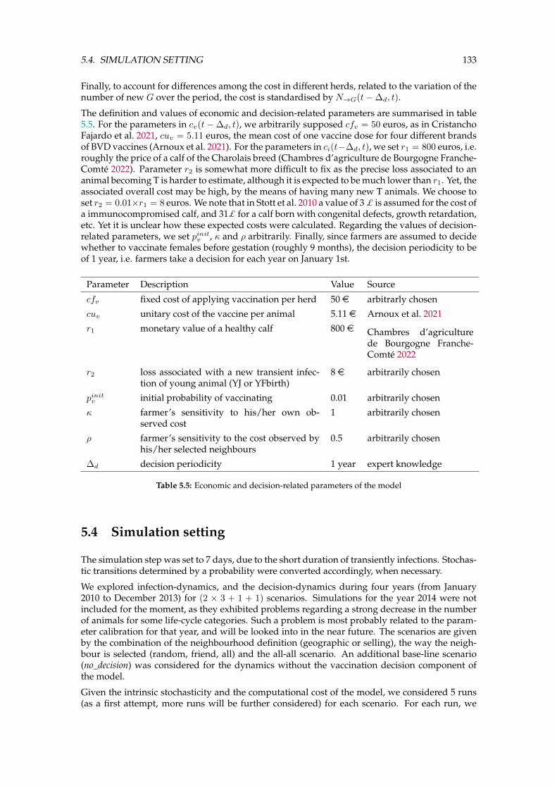
5.4. SIMULATION SETTING 133
Finally, to account for differences among the cost in different herds, related to the variation of thenumber of new G over the period, the cost is standardised by N→G(t−∆d, t).
The definition and values of economic and decision-related parameters are summarised in table5.5. For the parameters in cv(t−∆d, t), we arbitrarily supposed cfv = 50 euros, as in CristanchoFajardo et al. 2021, cuv = 5.11 euros, the mean cost of one vaccine dose for four different brandsof BVD vaccines (Arnoux et al. 2021). For the parameters in ci(t−∆d, t), we set r1 = 800 euros, i.e.roughly the price of a calf of the Charolais breed (Chambres d’agriculture de Bourgogne Franche-Comté 2022). Parameter r2 is somewhat more difficult to fix as the precise loss associated to ananimal becoming T is harder to estimate, although it is expected to be much lower than r1. Yet, theassociated overall cost may be high, by the means of having many new T animals. We choose toset r2 = 0.01×r1 = 8 euros. We note that in Stott et al. 2010 a value of 3 £ is assumed for the cost ofa immunocompromised calf, and 31£ for a calf born with congenital defects, growth retardation,etc. Yet it is unclear how these expected costs were calculated. Regarding the values of decision-related parameters, we set pinitv , κ and ρ arbitrarily. Finally, since farmers are assumed to decidewhether to vaccinate females before gestation (roughly 9 months), the decision periodicity to beof 1 year, i.e. farmers take a decision for each year on January 1st.
Parameter Description Value Source
cfv fixed cost of applying vaccination per herd 50 e arbitrarly chosen
cuv unitary cost of the vaccine per animal 5.11 e Arnoux et al. 2021
r1 monetary value of a healthy calf 800 e Chambres d’agriculturede Bourgogne Franche-Comté 2022
r2 loss associated with a new transient infec-tion of young animal (YJ or YFbirth)
8 e arbitrarily chosen
pinitv initial probability of vaccinating 0.01 arbitrarily chosen
κ farmer’s sensitivity to his/her own ob-served cost
1 arbitrarily chosen
ρ farmer’s sensitivity to the cost observed byhis/her selected neighbours
0.5 arbitrarily chosen
∆d decision periodicity 1 year expert knowledge
Table 5.5: Economic and decision-related parameters of the model
5.4 Simulation setting
The simulation step was set to 7 days, due to the short duration of transiently infections. Stochas-tic transitions determined by a probability were converted accordingly, when necessary.
We explored infection-dynamics, and the decision-dynamics during four years (from January2010 to December 2013) for (2 × 3 + 1 + 1) scenarios. Simulations for the year 2014 were notincluded for the moment, as they exhibited problems regarding a strong decrease in the numberof animals for some life-cycle categories. Such a problem is most probably related to the param-eter calibration for that year, and will be looked into in the near future. The scenarios are givenby the combination of the neighbourhood definition (geographic or selling), the way the neigh-bour is selected (random, friend, all) and the all-all scenario. An additional base-line scenario(no_decision) was considered for the dynamics without the vaccination decision component ofthe model.
Given the intrinsic stochasticity and the computational cost of the model, we considered 5 runs(as a first attempt, more runs will be further considered) for each scenario. For each run, we

134 CHAPTER 5. APPLICATION STUDY
considered that for a subset of 4% herds, 0.2% of their calves (YJ + YFbirth) were initially P. Thatis, 147 (=3685*0.04) herds were initially infected with 1 P calf each. Indeed, the initial total numberof calves (YJ + YFbirth) in the metapopulation for the year 2010 was 66549. Hence, the 0.2% Pcalves corresponded to 133 P calves in total, and each positive herd had 1 (= 133/147) P calf. Wedefined these initial conditions on the basis of the information from the animal health services(GDS: groupement de défense sanitaire) of Saône-et-Loire (GDS de Bourgogne - Franche-Comté 2022)for the year 2021, indicating 273 positive calves out of 184,930 tested (i.e. 0.2%), belonging to109 of the 2900 herds tested. That is 3.8% (=109/2900) of the herds had at least one P among thetested. We note however, that there was no measurement of vaccination practices in such study,which can partly explain such a low prevalence for a first generalised screening.
The P calf for each initially infected herd was chosen among the YJ or YFbirth, beef or dairyanimals of the selected herd, according to a multinomial distribution, where the probabilities ofthe P animal being a dairy/beef YJ/YFbirth animal were set proportional to the initial proportionof young animals in the chosen herd that were dairy/beef YJ/YFbirth. We remark that only herdsthat had initially at least 1 YJ or YFbirth animal were eligible to be initially infected, so as to ensurethe same initially infected P animals, and the same initial number of infected herds.
The simulation code of the model and parameter calibration can be found in the public repositorygithub.com/CristanchoLina/BVD_farmersdecisions.
5.5 Results
In the following, preliminary results over 5 runs are presented. As the number of runs is low,such results are not yet conclusive and additional explorations are needed.
Figure 5.8 presents infection dynamics in the metapopulation for each of the considered sce-narios. Without the vaccination component (no_decision scenario) the pathogen spreads quiterapidly, and at the end of the fourth year 50% of herds have at last 1 P calf. The proportion ofP animals among calves presents a seasonal behaviour, with waves whose peaks are attainedroughly at the end of each year, from the second year. The highest peak (almost 0.12) occurs atthe end of the third year. The final (at the end of the fourth year) proportion of P calves in themetapopulation is roughly 0.11.
Regarding the proportion of T animals in the metapopulation, figure 5.9 shows seasonal peaks,this proportion being almost 0.01 at the largest peak, attained between the second and thirdyear, and concerning 35% herds. Yet, between the third and the fourth year, the proportion of Tanimals in the metapopulation attains levels in the previous year. Even more, the proportion ofherds concerned by the presence of T animals increases (to 0.37) with respect to the highest levelregistered during the third year (0.35).
Regarding scenarios with decision-making, the first remark is that all of them achieve to de-crease pathogen spread (P and T animals and herds) when compared to the no_decision scenario(figures 5.8 and 5.9). Unsurprisingly, the group of scenarios were the pathogen spread is bettercontrolled is the one were farmers take into account all the information of their neighbourhood,through a weighted mean, constituted by the selling-all, geographic-all and all-all scenarios. Forthis group, the highest peak in the proportion of infected calves in the metapopulation (figure5.8(b)) is decreased to less than 0.03, attained at the end of the second year. In the followingyears, this proportion almost consistently decreases, even if a small peak is still observed beforethe end of the third year, until reaching less than 0.005 at the fourth year. Of the three scenarios inthis group, the worst control is obtained when decisions rely only on selling neighbours (selling-all scenario). In particular, figure 5.9 shows that it is the only scenario of this group for which apeak is clearly observed in the proportion of T animals (at almost 0.003), and in the proportion ofherds with T animals (0.15), in the third year. Similarly, the proportions of P animals and of herdswith P animals (figure 5.8) are higher than in the other two scenarios of the group, from the sec-ond year to the end of the fourth year. Indeed, the final values attained for this two proportionsare respectively almost 0.002 and 0.05 higher for the selling-all scenario than in the other two

5.5. RESULTS 135
0.00
0.05
0.10
0.15
0.20
0.25
0.30
0.35
0.40
0.45
0.50pr
opor
tion
of h
erds
with
P c
alve
s(a)no_decision
selling-friendselling-randomgeographic-friendgeographic-randomselling-allgeographic-allall-all
0.0 0.5 1.0 1.5 2.0 2.5 3.0 3.5 4.0year
0.000.010.020.030.040.050.060.070.080.090.100.110.12
prop
ortio
n of
P c
alve
s in
the
met
apop
.
(b)
Figure 5.8: Dynamics of BVD virus spread in the metapopulation. Proportion of herds with P calves (a) andproportion of P calves (out of all calves) in the metapopulation (b). Each colour represents the neighbour-hood (geographic or selling) and the way neighbours are selected for observation (random, friend or all),together with the all-all selection. Gray vertical lines represent decision times. Mean results and confidencebands (min to max) over 5 runs.
scenarios. Clearly, the performance of the all-all scenario is driven by that of the geographic-allscenario, as in the first both the geographic and the selling neighbours are taken into account.In particular, for both of these scenarios, the final levels of each of the fourth studied outputsare almost the same to the ones given by initial conditions. The group of scenarios where onlythe information of a single neighbour is taken into account at each decision time is found to be

136 CHAPTER 5. APPLICATION STUDY
0.00
0.05
0.10
0.15
0.20
0.25
0.30
0.35
0.40
prop
ortio
n of
her
ds w
ith T
ani
mal
s
(a)no_decisionselling-friendselling-randomgeographic-friendgeographic-randomselling-allgeographic-allall-all
0.0 0.5 1.0 1.5 2.0 2.5 3.0 3.5 4.0year
0.000
0.001
0.002
0.003
0.004
0.005
0.006
0.007
0.008
0.009
0.010
prop
ortio
n of
T a
nim
als i
n th
e m
etap
op.
(b)
Figure 5.9: Dynamics of BVD virus spread in the metapopulation. Proportion of herds with T animals(a) and proportion of T animals in the metapopulation (b). Each colour represents the neighbourhood(geographic or selling) and the way neighbours are selected for observation (random, friend or all), togetherwith the all-all selection. Gray vertical lines represent resource decision times. Mean results and confidencebands (min and max) over 5 runs.
in between the no_decision scenario and the previously mentioned group. With respect to thebaseline scenario in the scenarios of this group the proportion of herds with P calves shows alower increase, to attain roughly 0.3 at the end of the fourth year. For the proportion of P calvesin the metapopulation, the highest peak is reduced to 0.05, attained at the end of the third year(figure 5.8). A similar behaviour is observed for the proportion of herds with T animals, and theproportion of T animals in the metapopulation, whose highest peaks are respectively reduced to

5.5. RESULTS 137
0.30 and 0.008 (figure 5.9). As in the scenarios where all information was taken into account, thegeographic scenarios when using only one neighbour led to a better control of pathogen spreadwhen compared to the respective selling scenarios, even if the difference is not as striking aswhen using all neighbours. For both the geographic and selling neighbours, randomly choosingthe neighbour exhibited a better result in average, yet showed more variation.
Regarding vaccination dynamics, figure 5.10 shows that the proportion of herds that vaccinate in-creases from the initial value (roughly 0.01) to 0.25 in the geographic-random and the geographic-friend scenarios, to 0.27 in the selling-random and the selling-friend scenarios. The gap betweenthese two sets of scenarios increases over time, and at the end of the simulation (which corre-sponds to the beginning of a fifth year), in the geographic scenarios (random and friend) theproportion that vaccinates is around 0.42, while in the respective selling scenarios this propor-tion attains 0.52. No difference can be appreciated regarding the way farmers choose their ob-served neighbour (random or friend), once the neighbourhood is fixed. Regarding the scenarioswhere all information from the chosen neighbourhood is used, in the cases where the geographicneighbourhood was considered (either alone or with the selling neighbourhood), the proportionthat vaccinates increases to more than 0.98 from the first to the second decision time and staysat the same level throughout the years. Meanwhile, when considering solely the selling neigh-bourhood, this proportion increases to 0.7 at the beginning of the second year, and progressivelyincreases to attain roughly 0.9 at the beginning of the fourth year. Such a proportion is slightlyincreased at the beginning of a fifth year.
0 1 2 3 4year
0.0
0.1
0.2
0.3
0.4
0.5
0.6
0.7
0.8
0.9
1.0
prop
ortio
n of
her
ds th
at v
accin
ate
all-allgeographic-allselling-allselling-randomselling-friendgeographic-randomgeographic-friend
Figure 5.10: Dynamics of the proportion of herds that vaccinate. Each colour represents the neighbourhood(geographic or selling) and the way neighbours are selected for observation (random, friend or all), togetherwith the all-all selection. Mean results and confidence bands (min and max) over 5 runs.
The exploration of the vaccination patterns (for one run only) shows that in the scenarios wherefarmers use their geographic neighbours to decide, the proportion that never vaccinates is higherby at least 0.05 with respect to the scenarios where farmers use the selling neighbourhood, andthat the vaccination patterns where herds vaccinate most of the time are also more frequent in theselling scenarios (figure 5.11). Finally, figure 5.12 shows that, as expected, the proportion of herdsthat always vaccinate (excluding the first decision time) is higher (almost 1) in the geographic-alland the all-all scenarios, than in the selling-all scenario (0.7). Even if the pattern where herdsvaccinate from the second decision time is the next more frequent one for the latter scenario(almost 0.15), the proportion of herds that never vaccinate is higher (0.06) when compared to theother two scenarios (less than 0.02).
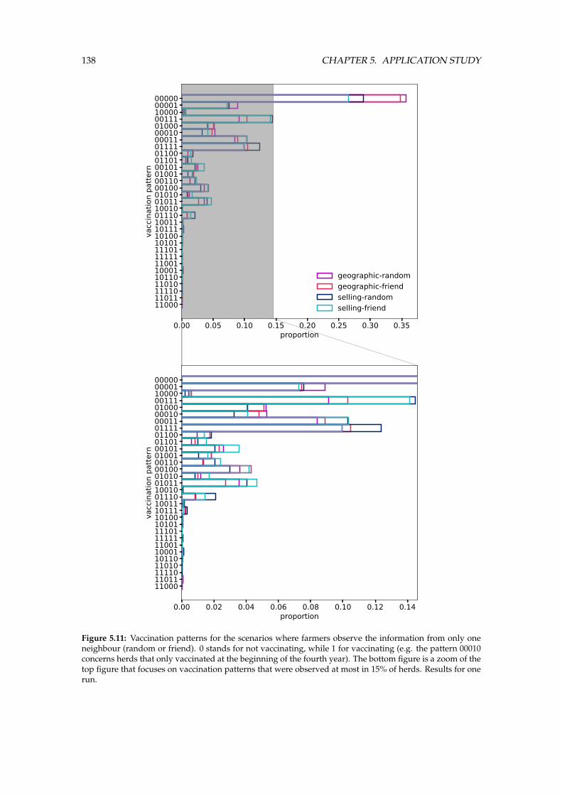
138 CHAPTER 5. APPLICATION STUDY
0.00 0.05 0.10 0.15 0.20 0.25 0.30 0.35proportion
00000000011000000111010000001000011011110110001101001010100100110001000101001011100100111010011101111010010101111011111111001100011011011010111101101111000
vacc
inat
ion
patte
rn
geographic-randomgeographic-friendselling-randomselling-friend
0.00 0.02 0.04 0.06 0.08 0.10 0.12 0.14proportion
00000000011000000111010000001000011011110110001101001010100100110001000101001011100100111010011101111010010101111011111111001100011011011010111101101111000
vacc
inat
ion
patte
rn
Figure 5.11: Vaccination patterns for the scenarios where farmers observe the information from only oneneighbour (random or friend). 0 stands for not vaccinating, while 1 for vaccinating (e.g. the pattern 00010concerns herds that only vaccinated at the beginning of the fourth year). The bottom figure is a zoom of thetop figure that focuses on vaccination patterns that were observed at most in 15% of herds. Results for onerun.

5.5. RESULTS 139
0.0 0.2 0.4 0.6 0.8 1.0proportion
0000000111011110101100001000110010011111001010100001001101110111000010011001000001101010101001100110
vacc
inat
ion
patte
rn
all-allgeographic-allselling-all
0.00 0.02 0.04 0.06 0.08 0.10 0.12 0.14proportion
0000000111011110101100001000110010011111001010100001001101110111000010011001000001101010101001100110
vacc
inat
ion
patte
rn
Figure 5.12: Vaccination patterns for the scenarios where farmers observe the information from all theirneighbours in the chosen neighbourhood (geographic and/or selling). 0 stands for not vaccinating, while1 for vaccinating (e.g. the pattern 00010 concerns herds that only vaccinated at the beginning of the fourthyear). The bottom figure is a zoom of the top figure that focuses on vaccination patterns that were observedat most in 15% of herds. Results for one run.
140 CHAPTER 5. APPLICATION STUDY
5.6 Discussion
In this chapter, the generic integrative model proposed in Cristancho Fajardo et al. 2021 (chapter3) is adapted for a real-life specific disease: the BVD. The adaptation concerned from one part,the economic-epidemiological cost on which farmers base their decisions. Indeed, the fact thatBVD model used is structured according to host-heterogeneities (in particular age and life-cycle),and the vaccine has an effect on vertical transmission, allowed for a more detailed evaluationof the economic and epidemiological consequences of vaccination decisions. Furthermore, asBVD virus can spread through different ways (geographical proximity or the trade network), theinitially proposed decision-mechanism was generalised to account for different neighbourhoodsand ways of selecting neighbours that can influence farmers decisions regarding the adoption ofa control measure (vaccination).
Preliminary simulations show that in all three scenarios where farmers observed at each decisiontime the previous actions and costs of all their neighbours (geographic and/or selling), BVD virusdid not spread as much as in the scenarios where only one neighbour was observed at a time(figures 5.8 and 5.9). Even more, for the scenarios where the full information of the geographicneighbourhood was observed, the prevalence of the pathogen was the same at the one givenat the beginning of simulations. Additionally, for the scenarios where farmers only choose asingle neighbour from which they obtain information, the geographic neighbourhood appearedto be slightly better for pathogen control than the selling neighbourhood (figures 5.8 and 5.9).Quite surprisingly, this occurs although under the geographic neighbourhood the proportion ofherds that vaccinate is almost always less than under the selling neighbourhood (figure 5.10), theproportion that never vaccinates is lower, and vaccination patterns where herds mostly vaccinateare less frequent.
Two main remarks can be made out of such observations. First, regardless of the chosen neigh-bourhood, using the full information of all neighbours at each decision time seems to have themost important impact for BVD control. Second, sharing information through the geographicneighbourhood seems to be consistently better for targeting herds that should get vaccinatedto reduce BVD virus spread. Meanwhile with the selling neighbourhood, even in cases wheremore herds slightly get vaccinated, vaccination is not adopted by some herds that are key for thecontrol of such spread.
It is to be stressed however, that such observations are not conclusive as many important aspectsof the simulations have been neglected for the moment. To the very short term, the calibration ofherd-specific parameters will be reevaluated, as some of these parameters presented unexpectedranges. In particular, the duration for animals in Fbirth presented some very high values thatmay unrealistically increase herd sizes in the simulations. For the proportion of culled and beefanimals, although their values were set to realistic values, in the future they will be calibratedfrom data and will depend not only on the herd, but also on the parity of the female. For themoment, this is not the case as in the calibration procedure the value of this parameter could notbe computed for several herds. This reevaluation of the herd-specific parameters may allow tostabilise the dynamics of the number of animals in each life-cycle category that are observed insimulations for the year 2014 (excluded in the present study). Once this issue is settled, the nextpoint to address will be the low number of runs (only 5 runs were considered for each scenario).More simulations should be performed so as to consider the observations conclusive. And anumerical analysis should be done regarding the values of decision-parameters (pinitv , κ and ρ) asthey were arbitrarily chosen. Indeed, qualitative remarks may not hold under different numericalsettings, and hence it will be of interest to explore the variation in results, as a function of thevariation in the values of these parameters. Finally, we could further explore and describe results,for example through an association between geographic position and vaccination patterns.
This work gives insights for the control of BVD virus spread through vaccination, by focusingon a zone densely populated with Charolais cattle, a breeding system for which vaccination hasproven to be a health measure of interest (Arnoux et al. 2021). The model represents how farmersvoluntary vaccination practices can be determined by their own past experiences (vaccinatingor not), and the information shared through their neighbourhood regarding other herds experi-

5.6. DISCUSSION 141
ences.
Regarding the limitations of this study (excluding those mentioned before, as they will soon beaddressed), we may include the same one made for the original integrative model in (Cristan-cho Fajardo et al. 2021) (chapter 3) regarding the fact that in the model farmers perfectly observecosts associated to their own and their neighbours decisions. Additionally, farmers consider inthe same way the observations of any of their chosen neighbours. In reality, farmers could givegreater weight to the observations made by their ’closer’ neighbours, i.e. account for their ge-ographic neighbours proportionally to the distance to their herd, and account for their sellingneighbours proportional to the amount of animals sold. Through this mechanism, the modelcould consider an additional strategic behaviour of farmers, as they could better account forhow the vaccination practices of their neighbours can impact the health status of their own herd.Finally, regarding the BVD virus spread model itself, we assumed that the metapopulation wasinitially infected, but that there was no risk of introduction of the virus from outside the metapop-ulation. As the area modelled is not that large, this assumption could be revisited and exposureto trade and geographic neighbours from other areas could be accounted for.


Chapter 6
Conclusions and perspectives
Contents6.1 Main contributions . . . . . . . . . . . . . . . . . . . . . . . . . . . . . . . . . . . 143
6.1.1 Integrative model for pathogen spread over an animal trade network ac-counting for farmers’ dynamic decisions regarding the adoption of a healthmeasure . . . . . . . . . . . . . . . . . . . . . . . . . . . . . . . . . . . . . 144
6.1.2 Strategies for the dynamic resource allocation of a limited resource forcontrolling disease spread on a metapopulation network . . . . . . . . . . 144
6.1.3 Study on farmers’ vaccination decisions integrated in a model of BVD’sspread at a large scale . . . . . . . . . . . . . . . . . . . . . . . . . . . . . . 145
6.2 Perspectives . . . . . . . . . . . . . . . . . . . . . . . . . . . . . . . . . . . . . . . 1456.2.1 On decentralised decision-making . . . . . . . . . . . . . . . . . . . . . . . 1456.2.2 On centralised decision-making . . . . . . . . . . . . . . . . . . . . . . . . 1476.2.3 On decentralised and centralised decision-making . . . . . . . . . . . . . 148
6.3 Conclusion . . . . . . . . . . . . . . . . . . . . . . . . . . . . . . . . . . . . . . . . 149
This thesis is concerned with the dynamics of infectious diseases spreading on a large metapop-ulation network, and the dynamic decision-making processes there can exist regarding the adop-tion of control measures to contain such spread, particularly in a context of livestock endemicdiseases spreading through trade. In particular, in such a multi-agent framework, there can bedynamic decisions that are taken locally (i.e. by the agents of the system themselves), and/ordynamic decisions taken in a centralised manner (i.e. by a central authority).
Although in epidemiology, a large diversity of mechanistic mathematical models are used fordescribing and predicting the spread of infectious diseases, the precise study of decision-makingin this context is most often neglected, particularly for the management of livestock diseases (Hi-dano et al. 2018). On the one hand, the behaviour of the individuals with a decisionary aptitudein the system where the pathogen spreads is usually not taken into account at all. When it is, thefocus is often on how a certain decision or behaviour could impact disease spread, but not onhow the behaviour itself can emerge as a function of the infection dynamics (Wang et al. 2016).On the other hand, regarding decisions made by a central entity for an optimal management ofthe disease, their study most often concerns unstructured and/or relatively small populations,as the solution to a most general problem is computationally intractable (Nowzari et al. 2015).
6.1 Main contributions
In the context described above, this thesis proposed two methodological contributions, and onecontribution regarding an application study. In the following, each of these contributions isbriefly summarised.
143

144 CHAPTER 6. CONCLUSIONS AND PERSPECTIVES
6.1.1 Integrative model for pathogen spread over an animal trade networkaccounting for farmers’ dynamic decisions regarding the adoption of ahealth measure
The first contribution (Chapter 3) concerned an integrative model of pathogen spread on an an-imal trade metapopulation network, that accounts for farmers’ voluntary decision-making re-garding the adoption of a health control measure against infection in their own herd. The epi-demiological component is built upon a stochastic SIR intra-herd model with demography, thataccounts for inter-herd animal transfers. The decision-making component consists in settinga dynamic decision problem under uncertainty, and proposing a dynamic decision-mechanismthat accounts for farmers’ stochastic behaviour, learning, and strategic imitation dynamics. Thus,there is a dynamic feed-back loop between the two components, as the control decisions are func-tion of the observed disease spread, and the disease spread is impacted at its turn by the decisionspreviously taken. The model was detailed and simulated for a specific measure (vaccination).The infection and vaccination decision dynamics for contrasted scenarios were studied, and therobustness regarding the values of the model’s parameters was assessed. Experiments showedthat decision related parameters highly impact vaccination decisions, and therefore the course ofthe disease spread.
Previous studies (Bauch 2005; Fu et al. 2010) were pioneers in accounting for real-life aspects ofhuman behaviour regarding vaccination against human diseases, such as stochastic behaviourand imitation. Yet, such type of study has rarely considered an explicit learning process for rep-resenting human-decision making. Furthermore, these works had not yet been adapted for thespecificities related to the management of livestock diseases. Hence, the first model proposedin this thesis is a significant step towards accounting for human behaviour in epidemiologicalmodels. Additionally, its generic formalisation allows it to be relevant for a variety of epidemio-logical models or measures. Potential extensions and uses can be further facilitated by the publicavailability of the simulation code.
6.1.2 Strategies for the dynamic resource allocation of a limited resource forcontrolling disease spread on a metapopulation network
The second contribution (Chapter 4) concerned the optimisation of a social planner’s decisionsregarding the allocation of a limited resource among the sub-populations of a metapopulationnetwork. This problem was studied for a livestock disease spreading on an animal trade net-work. Again, for each sub-population (herd) of the network, a stochastic SIR intra-herd modelwith demography was used, accounting for inter-herd animal transfers and grounded on data forits non epidemiological components. The contribution is based on an extension to this metapop-ulation framework of an approach initially proposed for networks without epidemiological-demographic within-node dynamics (i.e. a node of the network corresponded to an individual,not a sub-population). The approach consists in deriving analytic scores minimising an approx-imated variant of an objective function and then dynamically allocating the resource to eachsub-population according to their ranking given by the sub-populations scores, and the limitedamount of resource. Such optimised scoring functions were obtained for two different objectivefunctions, and for two different types of resources (vaccine and treatment). Their performancesin containing disease dynamics and their relevance in practice for allocating the resource wereassessed, along with the ones of several heuristic scores. It was shown that the analytic scoringfunctions can allow for a significant control of the pathogen spread, although they are not al-ways truly optimal in practice. However, they perform in general much better than the scoringfunctions based only on information on demographic or trade data, as in most of the evaluatedscenarios, information on epidemiological status appeared as necessary to achieve disease erad-ication.
This work represents an advance into optimising socially planned interventions in a complexsystem of disease propagation on a large metapopulation network. Indeed, related studies refereither to small metapopulation networks (e.g. Mbah et al. 2011), or to large non metapopulation

6.2. PERSPECTIVES 145
networks (e.g. Wijayanto et al. 2019). The same approach could also be used for different epi-demiological compartmental models in the metapopulation framework. Moreover, other mea-sures can be studied leading to other specific greedy scores, to be obtained. Finally, like for thework in Chapter 3, the simulation code was made available in a public repository.
6.1.3 Study on farmers’ vaccination decisions integrated in a model of BVD’sspread at a large scale
The final contribution (Chapter 5) consists of an application and extension of the integrativemodel in Chapter 3, to a specific real-life disease (BVD), supposing that farmers’ decision-makingcan be influenced in other ways than the one initially considered. In this application, the method-ological framework was extended to consider that farmers can make decisions as a function ofthe decisions and observations of their neighbours, not only in the animal trade network, as as-sumed in the original generative model, but also in their geographical neighbourhood (i.e. basedon geographical proximity to other farms). Furthermore, several alternative ways on how theneighbours are chosen were evaluated. Finally, this ongoing work highlights how the compo-nents of the integrative model can be adapted to the study of a different type of epidemiologicalmodel (an individual-based model) for the control of a real-life disease, in this case BVD, throughthe adoption of a health measure (vaccination) that has been proven to be of interest for certaincontexts (Arnoux et al. 2021).
6.2 Perspectives
The assumptions made throughout this thesis are accompanied by some advantages and limita-tions. Such limitations can be of inspiration for subsequent works as they can open up to perspec-tives of interest. In the following, certain perspectives are described. Some of these perspectivesconcern elements mentioned in the discussions of previous chapters, that are here summarisedor deepened, while other perspectives are more detailed as they can have a wider opening.
6.2.1 On decentralised decision-making
First, regarding the works relative to farmers’ decision-making (Chapters 3 and 5), four pointscould be addressed: observation of costs, variation of the decision algorithm, parameter robust-ness, and the consideration of more relevant health measures.
6.2.1.1 Noisy observation of costs
The epidemiological and farmer’s decision-making components are linked through an economiccost that is function of the epidemiological dynamics following the previous decision, and onwhich the following decision is taken. For updating their decisions, it was supposed that farmerscould perfectly observe the costs associated to their own previous action and the previous actionsand associated costs of their neighbours, either by observing the number of new infected animals,or by directly observing the associated financial loss.
However, it can be a strong assumption that the observed cost precisely corresponds to the lossassociated with the true number of new infections within the period. In reality, even if farm-ers could observe an increase/decrease in the number of infected animals (for example, throughsymptomatic animals, which would already be a noised signal of the number of infected ani-mals), they would probably not be able to exactly know the number of new infections in theherd, i.e. distinguishing infected animals whose infection occurred within the herd, from im-ported infected animals (whose health status could reflect a decision of the origin herd), and also

146 CHAPTER 6. CONCLUSIONS AND PERSPECTIVES
because most of the time infection remains undetected. Furthermore, farmers most probablyonly have a rough idea of the observed costs of their neighbours.
Relaxing this hypothesis could impact the observed decision patterns and the local or overall dis-ease dynamics. To this end, the cost could be reformulated to be dependent not on the number oftrue new infections, but on the increase of infected animals with respect to the previous decisionperiod, i.e. assuming that farmers perfectly observe prevalence, not incidence. Alternatively, anappropriate additive noise could be accounted for in observed number of infections (or in theobserved increase in the number of infected animals) within the period. Such an additive noisecould be, for example, distributed as a binomial random variable whose parameters would needto be calibrated.
6.2.1.2 Variations of the decision-making algorithm
An algorithm intended to represent farmers’ decision-making process was proposed and evalu-ated within the context of both a theoretical and a real-life infection relying on real-life aspects ofhuman decision-making such as learning and strategic imitation. Although the algorithm con-siders heterogeneity in decision outcome, it has a structural homogeneity (i.e. all farmers havethe same decision-making process). In particular, for vaccination, the same values for decision-related parameters were assumed: same initial probability of vaccinating, same sensitivity totheir own observed costs and same sensitivity to the observed costs of neighbours. Aside fromthe fact that it is actually unknown to what extent this algorithm reflects the true decision processof a typical farmer, considering that such a typical farmer is a representative decision-maker forall the farmers in the trade network might be a strong assumption, as farmers could have dif-ferent values of decision-related parameters, or even alternative decision-making processes. Yet,instead of considering more than one decision-making mechanism present in the metapopula-tion, a simple option to address this limitation would be for instance to assign, on the basis of theproposed decision-making mechanism, a low probability of applying the measure to half of thefarmers, and a high probability to the other half, which could allow for additional explorations onthe decision patterns. More generally, the hypothesis could be alleviated by considering differentdecision profiles, using a distribution for each of the three previously mentioned parameters.
Another assumption in the farmers’ decision process was to consider in the same way any neigh-bour whose observation of actions and associated costs is explicitly included in the decision. In-deed, the neighbours are chosen uniformly at random. Furthermore, the sensitivity to the resultsof any neighbour is the same.
Although this seems an acceptable hypothesis as a starting point, more potentially realistic as-sumptions could be made. In particular, the probability of selecting a given neighbour in thetrade network could be proportional to the amount of animals purchased from the neighbour.Such a weight could also be considered for the parameter regarding the sensitivity to neigh-bour’s observed costs. Hence, farmer’s decision-making would be not only based on the costsobserved by his/her neighbours, but would also, in a way, take into account the impact thatthe neighbours’ decisions may have on his/her own herd as a function of the amount of animalspurchased. That is, by integrating the potential risk of importing infected animals, farmers mightfocus on the health practices of the herds from which they purchase most animals. A similar ap-proach could be taken for the geographical neighbour, weighting by the geographical distancebetween herds. This could, in principle, strengthen the impact that a different neighbourhood,or a different way of choosing the neighbour, may have.
6.2.1.3 Robustness to parameter values
The robustness of the initial integrative model presented in chapter 3 to the parameters was as-sessed through several sensitivity analysis experiments. However, the adaptation of the costfunction for vaccination decisions on BVD involved new parameters with respect to the originalgeneric model. The values of some of the parameters (the decision-related ones) were arbitrarily

6.2. PERSPECTIVES 147
chosen. Therefore, results and conclusions may be different for other values of such parame-ters. Additionally, the impact of the variation of the tested parameters of the model might havechanged in the presence of new parameters (Saltelli et al. 2008).
Hence, a new sensitivity analysis should eventually be performed for this new model, in partic-ular on the new parameters, in order to evaluate the qualitative impact of their variation on theconclusions of this work.
6.2.1.4 More relevant field measures
The generic formulation of the integrative model allows it to be adapted to different epidemio-logical state structures, including other compartmental models, as evidenced by the BVD appli-cation study. Furthermore, the adaptation could also concern the use of other types of controlmeasures.
However, only vaccination was explicitly modelled and simulated. Although this seemed themost important measure to look at for endemic unregulated diseases, other measures more rel-evant in the field could be evaluated. In particular, for the application study on BVD, a classicalmeasure is to test animals at birth in order to detect persistently infected calves on ear tag sam-pling. Such a policy could be modelled (like vaccination in chapter 5) by making a decision at thebeginning of each period of time, and applying the measure at each birth occurring within thisperiod. Another measure consisting in changing pasture practices could be considered: delay-ing the pasture period according to the economic losses related to infected animals. Consideringsuch a measure could widen the use of this model to other administrative areas, where vacci-nation might not to be an appropriate measure for controlling BVD, e.g. the French region ofBrittany, mainly populated with dairy cattle, as BVD has been controlled in dairy herds withoutusing vaccination. Additionally, as opposed to countries that use vaccination as the BVD eradica-tion plan (e.g. Germany, Belgium, Ireland, Scotland), some countries (e.g. Switzerland, Austria)have chosen an approach without vaccination (Moennig et al. 2018), since their policies are basedon the detection of BVD through serology, and vaccination interferes with serological results.
Depending on the measure, the adaptation of the decision-making model, and in particular ofthe economic-epidemiological cost, may not be so straightforward. For example, for test-and-cull, bulk tank milk could be followed to highlight new virus circulation in a herd, and then adecision could be taken as a function of such measurement. This could also imply that decisionsare not taken at regular time steps, but following a change in herd status based on such screening(see section 6.2.3.2 for a discussion on this point).
6.2.2 On centralised decision-making
Second, concerning the work on centralised dynamic resource allocation on a large metapopula-tion network (Chapter 4), three aspects could be considered: the availability of health informa-tion, the observation of a sub-network, and the dynamic nature of the network.
6.2.2.1 Noisy or partial health information
For the resource allocation problem, it was assumed that the social planner could exactly com-pute the scores (heuristic or optimised) based on real-time health information. However, in thefield, there is rarely such detailed information regarding the health-status of the farm, particu-larly for endemic animal diseases. Hence, such scores may not be possible to be observed, inparticular those based on real-time intra-herd incidence or prevalence.
To overcome this limitation, an option on the basis of the work presented in this thesis wouldbe to build a composite score as a linear combination of uncorrelated scoring functions with nonecessarily highest performance but that are likely to be observed.

148 CHAPTER 6. CONCLUSIONS AND PERSPECTIVES
6.2.2.2 Sub-network
Instead of having partial information, like in the previous point, it may be possible to have noinformation at all for some sub-populations (health-related or not), and the resource may be hardto allocate for some of them (deployment constraints). A less restrictive hypothesis would be toassume that the social planner can only observe and access a sub-network for the resource alloca-tion. This perspective could be addressed in the light of the work in Fekom et al. 2020 regarding arestricted dynamic resource allocation (RDRA) problem, in which at each time the social planner canallocate the resource only among random sample of reachable nodes of a (non metapopulation)network.
6.2.2.3 Dynamic network
In chapter 4, new optimisation based scores were found for allocating a resource (vaccine ortreatment) among the sub-population of an arbitrary metapopulation network.
However, even if these new scores were evaluated through simulation on a dynamic metapopu-lation network, they were built on a static aggregated view of such network. Although this maybe seen as an advantage, as their performance does not depend on real-time information on thetopology of the network, scores that would actually take into account the time-varying struc-ture of the network could potentially achieve better performances that the ones observed for thederived scores. The possibility of finding such scores could be explored with a new formal anal-ysis. If obtained, such scores could be compared by simulation to the scores initially derived andgive insights regarding the importance of the availability of real-time topological information forresource allocation in a metapopulation network.
6.2.3 On decentralised and centralised decision-making
6.2.3.1 Coupled centralised-decentralised decision-making
It would be of interest to revisit the assumption of separating the social planner’s and the farmers’decision-making. This could be done by considering in the resource allocation problem, thatfarmers’ behaviour is not limited to doing what the social planner finances. The objective wouldbe to couple the farmers’ decision model, and the social planner’s resource allocation problemand proposed strategies. For a complete coupling, the planner should take into account farmers’behaviour and vice-versa.
Regarding the social planner, a possible approach is to consider that a score-based strategy isapplied only on a group of sub-populations. This is not necessarily the same framework as therestricted dynamic resource allocation (RDRA) problem, as here the social planner can observeand have access to the whole metapopulation network, yet decides not to allocate the resource tosome sub-populations so that farmers control the pathogen spread themselves, to a certain extent.There are several choices for the eligible group for resource allocation, yet the implications of oneor another should be carefully studied (Zhang et al. 2013). A first simple approach, recently takenfor a human theoretical disease in Meng et al. 2022, would be to allocate the resource on somesub-populations based on a predefined score, and leave the rest of the sub-populations decidewhether to apply the measure or not, i.e. not actually coupling the decision-making processesbut only assuming they occur in a certain order. As an alternative, it could be assumed thatthe social planner would only allocate the resource to the sub-populations that did not applya control measure for themselves. However, in both options, counter-productive effects shouldbe taken into account, as such options can represent an incentive for farmers not to apply themeasure for themselves. Indeed, farmers could anticipate that they can be indirectly or directlyprotected from infection through the resource allocation performed by the social planner, even ifthey decided not paying the price of applying the measure. Another option could be to allocatethe resource for sub-populations that did apply the measure (at the previous decision period),

6.3. CONCLUSION 149
hence rewarding them. This could, in principle, be an incentive for farmers to further applythe measure, but could cause overspending resources (e.g. the cost of increasing vaccinationcould be greater than the cost of infection) (Kuga et al. 2019). Finally, a more developed strategyfor resource allocation could be based (apart from the allocation score) on the full history ofinformation regarding control related practices of the farmers, similarly to what is proposed fora theoretical model of a human seasonal disease in (Ding et al. 2018).
A final important aspect to take into account on this matter is how to define decision times. Forexample, if farmers and the social planner make simultaneous decisions, the social planner mightallocate resources to herds that would have applied a measure for themselves. Yet, if decisionswere interspersed, farmers may change their decision in anticipation of the social planner’s re-source allocation policy.
Regarding farmers, independently of the strategy chosen by the social planner, a term could beadded in the cost function to decrease the probability of a farmer applying the measure if, at thelast decision step, the planner allocated the resource to the herd. Alternatively, farmers’ decision-making could be left unmodified, and it could be explored to what extent the social planner’sdecisions influence farmers’ decisions only through the bias of variations in pathogen spread.
6.2.3.2 Decision-step optimisation: when to allocate?
Either for farmers’ or social planner’s decision-making, a fixed heuristic value was consideredfor the decision-step ∆d, which for vaccination, also defines the duration of the vaccine efficacy.Even if this assumption is not unrealistic when compared to field practice for vaccination, othermanners to determine the decision step are more appropriate depending on the control mea-sure in mind (see section 6.2.1.4). These alternative ways of determining decision times rely onconsidering that decisions can be made asynchronously across herds. A first option would beto consider a decision step for each herd that is determined adaptively as a function of an ex-ternal input. A second, more elaborate option, would be to build an optimisation procedure todetermine when to take decisions. Such methodological variations of the model are not straight-forward, especially when considering the second option (i.e. determine the decision-step byoptimisation) together with the problem considered in this thesis (i.e. determine the resourceallocation by optimisation).
6.3 Conclusion
The work presented in this thesis provides insights on modelling and optimisation of the controlof pathogens spreading on animal trade networks, when such control is carried out voluntarilyby farmers or by a central authority. Through identifying and exploiting the bridges betweenepidemiology and fields related to control decisions in a multi-agent setting, important questionsand elements for such control at a large scale have been raised and addressed, either to modelthe voluntary behaviour of system agents, when they are humans, or to optimise the control ofthe system as a whole.
Research works on this topic are useful to better understand and predict real life phenomenathat are not only dependent on biological processes, but also on other aspects such as humanbehaviour or governmental decision-making. Such better understanding and predictions havethe potential of improving coordination among the different actors of the system. In particular,regarding the management of livestock diseases, a better coordination could ultimately accountfor the practices, interests and motivations of farmers, and at the same time allow for a betterglobal control of the pathogen spread on complex networks through animal trade.
To this end, an integrative point of view seems to be particularly appropriate for such a cross-sectional problem. This should account not only for approaches from epidemiological field, butalso from all the fields that study, in some way or another, decision-making. Indeed, in epidemi-ology, the control of pathogens could be improved by the expertise of the other fields regarding

150 CHAPTER 6. CONCLUSIONS AND PERSPECTIVES
decision-making, while such fields could be enriched by the complexity of the problems dealtwith in epidemiology.

Chapter 7
Résumé en français: contexte etcontributions de la thèse
Contents7.1 Contexte . . . . . . . . . . . . . . . . . . . . . . . . . . . . . . . . . . . . . . . . . 151
7.1.1 Gestion dynamique de la propagation d’une maladie sur un réseau com-plexe . . . . . . . . . . . . . . . . . . . . . . . . . . . . . . . . . . . . . . . 151
7.1.2 Maladies endémiques du bétail se propageant par le biais du commercedes animaux . . . . . . . . . . . . . . . . . . . . . . . . . . . . . . . . . . . 153
7.2 Contributions . . . . . . . . . . . . . . . . . . . . . . . . . . . . . . . . . . . . . . 1557.2.1 Modèle intégratif pour la propagation d’agents pathogènes sur un réseau
de commerce d’animaux rendant compte des décisions dynamiques desagriculteurs concernant l’adoption d’une mesure sanitaire . . . . . . . . . 155
7.2.2 Stratégies pour l’allocation dynamique d’une ressource limitée pour lagestion de la propagation des maladies sur un réseau de métapopulation 156
7.2.3 Etude sur les décisions de vaccination des agriculteurs intégrées dans unmodèle de propagation de la diarrhée virale bovine à grande échelle . . . 157
7.3 Conclusion . . . . . . . . . . . . . . . . . . . . . . . . . . . . . . . . . . . . . . . . 157
7.1 Contexte
L’objectif principal de cette thèse était d’identifier, d’adapter et de construire les approches appro-priées pour modéliser et optimiser efficacement l’adoption de mesures de gestion pour limiterla propagation d’une maladie sur un grand réseau de métapopulation. Le réseau a été spéci-fiquement considéré comme un réseau commercial de bétail à travers lequel la maladie peut sepropager entre fermes dans une certaine région.
7.1.1 Gestion dynamique de la propagation d’une maladie sur un réseau com-plexe
La structure des contacts entre individus est un élément clé à prendre en compte pour mieuxcomprendre la propagation de maladies infectieuses et finalement pour la contrôler (Keeling etal. 2005). Ceci est particulièrement vrai pour la transmission de maladies entre plusieurs sous-populations sur une grande zone géographique. Bien que les agents pathogènes puissent êtretransmis entre les sous-populations de plusieurs façons, en fonction de l’agent pathogène et ducontexte (par exemple, environnement partagé, vecteurs animaux sauvages), l’une des voies detransmission les plus courantes est le déplacement d’individus infectés (Danon et al. 2011).
151

152 CHAPTER 7. RÉSUMÉ EN FRANÇAIS: CONTEXTE ET CONTRIBUTIONS DE LA THÈSE
En effet, les mouvements d’individus entre différentes sous-populations forment une structureappelée réseau de métapopulation (Keeling et al. 2005), dans laquelle les noeuds sont les sous-populations et les liens sont représentés par les mouvements. Un tel réseau est dirigé, car les indi-vidus se déplacent d’une sous-population à l’autre; pondéré, car il y a un poids (flux d’individus)associé à chaque lien; et dynamique, car les flux changent dans le temps (les liens ne sont paspérennes et/ou le nombre d’individus qui se déplacent entre deux sous-populations peut varierdans le temps.). De plus, lorsque les coordonnées spatiales sont explicitement prises en compte,les liens peuvent connecter des sous-populations même s’il n’y a pas de proximité géographiqueentre elles (réseau spatial).
En particulier, ce contexte permet de décrire deux phénomènes spécifiques. D’abord, l’introductiond’un agent pathogène dans une sous-population où il n’était pas présent, appelé événement decolonisation (Donahue et al. 2008). Le second type de phénomène est la persistance de la propa-gation d’un pathogène à grande échelle malgré son extinction à petite échelle, ce que l’on appelleun rescue effect (effet de sauvetage) (Brown et al. 1977). Il s’agit d’un concept bien connu en écolo-gie: des épidémies de courte durée ont lieu au niveau des sous-populations, mais la maladie semaintient à grande échelle en raison des interactions entre les sous-populations.
La question de la gestion d’une maladie se propageant sur un réseau aussi complexe se pose rapi-dement. Le système est intrinsèquement dynamique (en raison des mouvements des individus,des changements démographiques des sous-populations au fil du temps et de la propagationde la maladie), tout comme peut l’être la prise de décision. En effet, la gestion de maladies in-fectieuses dans la vie réelle est généralement effectuée par des décisions répétées dans le temps(campagnes de vaccination, restrictions temporelles des mouvements, etc.)
De plus, étant donné que le réseau est vaste et englobe de nombreuses sous-populations, lesdécisions concernant l’adoption de mesures de gestion pour réduire la propagation de la mal-adie peuvent être prises à deux niveaux différents. D’une part, s’il existe un agent décisionnelhumain associé à chaque sous-population du système, nous sommes en présence d’un prise de dé-cision humaine décentralisée. D’autre part, la gestion peut être assurée par un planificateur central,généralement un planificateur social. On parle alors de prise de décision centralisée du planifica-teur social. La distinction entre ces deux types de prise de décision est importante car, selon ledécideur, les décisions répondront à des motivations différentes. En outre, la prise de décisionhumaine décentralisée peut naturellement introduire un comportement stratégique et une miseen œuvre hétérogène des mesures de gestion parmi les nombreuses sous-populations du système(Kreps 1997).
Dans ce contexte, l’utilisation d’approches mathématiques appropriées pour décrire et contrôlerun tel système s’avère très utile. En particulier, les modèles épidémiologiques mécanistes peu-vent être des instruments pour représenter et comprendre le système complexe impliqué dansla propagation des agents pathogènes (Keeling et al. 2011). Comme le comportement humainpeut avoir un rôle majeur dans la propagation des maladies, en particulier pour celles dont lagestion est volontaire, la prise en compte des décisions liées à la gestion de la propagation peutaugmenter la précision de ces modèles, et donc aider à mieux comprendre et prédire cette propa-gation. De plus, sur la base de ces modèles mécanistes, il est possible de concevoir des stratégiespour la gestion de la propagation de maladies infectieuses (Manfredi et al. 2013). Cependant,dans le processus de modélisation et de la gestion d’un tel système, des défis méthodologiquesse posent lorsqu’il s’agit de prendre en compte les décisions dynamiques, qu’elles soient prisespar un planificateur social ou par les agents humains du système.
Bien que la modélisation mathématique mécaniste soit de plus en plus utilisée dans l’étude desmaladies infectieuses, la plupart des modèles existants dans la littérature ne font pas référenceaux décisions volontaires d’agents en interaction (Wang et al. 2016), ou ils ne considèrent pas quele processus de prise de décision est dynamique (Rat-Aspert et al. 2010). En outre, les approchesclassiques considèrent les humains comme des particules (Manfredi et al. 2013), ou lorsque les as-pects économiques sont pris en compte les agents sont considérés comme parfaitement rationnels(par exemple Bauch et al. 2004; Zhang et al. 2012), ce qui est une hypothèse forte et controverséepour la prise de décision humaine (Wang et al. 2016). Enfin, les influences entre les décisions desagents sont souvent négligées (Shi et al. 2019), malgré le fait qu’il s’agisse d’une caractéristique

7.1. MALADIES ENDÉMIQUES DU BÉTAIL SE PROPAGEANT PAR LE BIAIS DU COMMERCE153
importante du comportement humain, notamment en ce qui concerne la gestion des maladies dubétail (Hidano et al. 2018).
Par conséquent, du point de vue de la modélisation, un premier défi consistait à construire uncadre qui formalise de manière appropriée la relation entre la dynamique de la propagation d’unemaladie sur un grand réseau de métapopulation et la dynamique de l’adoption volontaire demesures de gestion dans chaque sous-population, tout en tenant compte de considérations psy-chologiques, cognitives ou économiques pertinentes.
Un deuxième défi consistait à développer ou adapter des méthodes qui puissent être effective-ment appliquées pour gérer de manière optimale la propagation de la maladie sur le réseau.Parmi les considérations à prendre en compte, l’une des plus importantes concernait la complex-ité computationnelle du problème. En effet, il s’agissait du principal défi pour la résolution d’unproblème d’optimisation dans le cadre actuel, en raison de la grande dimension du réseau (Pelliset al. 2015).
Pour cette raison, les recherches sur ce sujet se sont principalement concentrées sur deux typesde situations, soit le réseau est petit (par exemple Chernov et al. 2020; Viet et al. 2018), soit il s’agitd’un grand réseau d’individus, c’est-à-dire qu’il ne s’agit pas d’une métapopulation où chaquenoeud du système a une dynamique interne propre (par exemple Lorch et al. 2018; Zhang et al.2015). Dans le premier cas, les études se fondent le plus souvent sur les processus de décisionde Markov (MDP) (Puterman 2014) ou sur la théorie des jeux (Myerson 1997). Dans le second,les auteurs ont généralement recours à des approximations de type champ moyen inspirées de laphysique (Lasry et al. 2007), qui peuvent être inappropriées si l’on souhaite prendre en compteune rationalité limitée ou des hétérogénéités entre les agents. Cela peut concerner par exemplel’influence qu’un agent peut avoir sur les décisions des autres agents, qui peut être déterminéepar sa place dans le réseau.
Les avancées dans ces deux objectifs, modélisation et optimisation, contribuent à mieux com-prendre les différentes caractéristiques du système complexe impliqué dans la propagation desagents pathogènes sur un tel réseau, et finalement à le contrôler efficacement.
7.1.2 Maladies endémiques du bétail se propageant par le biais du commercedes animaux
Les modalités de transmission des maladies entre individus sont proches que l’on considère deshumains ou des animaux (faune sauvage ou bétail), mais quelques différences existent néan-moins. Tout d’abord, les humains ont tendance à se déplacer librement entre les foyers, leslieux de travail, les lieux d’étude, les villes, les pays, etc., tandis que le bétail reste générale-ment longtemps dans une exploitation avant d’en rejoindre une autre par le biais du commerced’animaux (Brooks-Pollock et al. 2015). Deuxièmement, les considérations économiques peuventêtre plus centrales pour la gestion des maladies du bétail que pour les maladies humaines, oùl’aspect santé publique prime généralement sur le reste. Ainsi, les avancées méthodologiquespour la gestion des premières ont en principe plus de chances de trouver l’adhésion des agentsde terrain.
Suite à la crise de l’encéphalopathie spongiforme bovine (communément appelée maladie de lavache folle) qui a eu lieu notamment au Royaume-Uni entre 1986 et 2000, les pays européensmaintiennent des bases de données nationales concernant les mouvements de bovins entre ex-ploitations. En effet, les mouvements d’animaux occasionnés par les échanges constituent unevoie majeure de transmission des agents pathogènes du bétail entre les exploitations (Fèvre et al.2006), par exemple la paratuberculose (Beaunée et al. 2015), la fièvre aphteuse (FMD) (Fergusonet al. 2001) et la tuberculose bovine (bTB) (Donnelly et al. 2003).
Ces échanges se font directement entre deux exploitations, ou peuvent passer par des structuresintermédiaires. Les échanges directs concernent généralement des exploitations géographique-ment proches, de sorte que la propagation de la maladie est surtout concentrée dans une petitezone géographique. Par ailleurs, les mouvements d’animaux peuvent se faire via des marchés

154 CHAPTER 7. RÉSUMÉ EN FRANÇAIS: CONTEXTE ET CONTRIBUTIONS DE LA THÈSE
ou des centres de rassemblement. Ces structures facilitent le commerce d’animaux à une grandeéchelle géographique, en augmentant les échanges d’animaux provenant d’une exploitation géo-graphiquement éloignée de l’exploitation de destination. Elles augmentent donc encore le risquede transmission d’agents pathogènes sur de vastes zones (Robinson et al. 2007). La figure 7.1 il-lustre l’exemple d’un réseau commercial de bovins formé par les mouvements d’animaux laitiersentre les troupeaux de bovins, qui s’est produit en 2009 en France selon la base de données na-tionale d’identification (BDNI), qui enregistre l’histoire de vie de chaque bovin de la naissanceà la mort. Cette figure met en évidence les échanges d’animaux géographiquement proches etéloignés qui peuvent avoir lieu dans un réseau commercial d’animaux, et par lesquels une prop-agation de la maladie est susceptible d’atteindre l’ensemble du territoire français.
Figure 7.1: Flux commerciaux de bovins (animaux laitiers uniquement) pour l’année 2009 en France, à partirde la base de données française d’identification des bovins. Chaque nœud est une commune (la plus petiteunité administrative française). Source: Gaël Beaunée.
Une maladie qui se propage par le biais des échanges entre animaux a de fortes chances de de-venir endémique dans une zone donnée, c’est-à-dire présente à une prévalence donnée (générale-ment modérée) dans l’ensemble de la population pendant de longues périodes (Carslake et al.2011). Comme mentionné pour le cadre général des métapopulations, dans les métapopulationsanimales, la persistance de la maladie peut être observée à grande échelle par le biais de deuxprocessus. Premièrement, une longue durée d’infection dans une sous-population donne lieu àune longue infection de la métapopulation. Ensuite, la persistance peut être observée s’il existeun rescue effect dû aux interactions entre les sous-populations (voir par exemple Jesse et al. 2008).
Par ailleurs, une maladie peut présenter une dynamique épidémique, ce qui signifie par définitionque l’on observe une propagation importante et rapide sur une courte période de temps. Desexemples de ce type sont la fièvre aphteuse (Ferguson et al. 2001), la peste porcine africaine(PPA) (Nigsch et al. 2013), et la grippe aviaire (Benincà et al. 2020). Pour une maladie donnée, ladistinction entre dynamique endémique et dynamique épidémique se fait à partir des donnéesde surveillance. Or, les données de surveillance détaillées sont principalement disponibles pourdes maladies qui ont déjà été qualifiées d’épidémiques (Carslake et al. 2011).
Une fois qu’une maladie est associée à une dynamique épidémique, des efforts politiques impor-tants sont déployés afin de l’éradiquer. En particulier, les politiques publiques ciblent générale-ment les maladies épidémiques du bétail en réglementant leur gestion de manière obligatoire.Dans ce cas, on dit que la maladie est réglementée. En revanche, les maladies endémiques in-téressent généralement moins l’opinion publique et les décideurs politiques. Par conséquent,leur gestion est souvent laissée aux initiatives individuelles ou locales, et n’est donc pas obliga-toire, ce qui fait que les maladies endémiques sont le plus souvent non réglementées.

7.2. CONTRIBUTIONS 155
Néanmoins, comme elles persistent sur de longues périodes, les maladies endémiques peuventavoir une incidence cumulée importante, entraînant une réduction de la rentabilité économiquedes exploitations et du bien-être des animaux (Tomley et al. 2009). En outre, les zoonoses (lesmaladies infectieuses qui qui peuvent se propager entre animaux et humains) jouent un rôle ma-jeur dans le nombre croissant de maladies humaines émergentes (Lefrançois et al. 2014). En effet,au moins 60% des maladies infectieuses humaines émergentes sont des zoonoses et, en partic-ulier, plus de 30% des zoonoses infectieuses émergentes sont associées aux animaux destinés àl’alimentation (Otte et al. 2021). Par conséquent, la gestion de maladies endémiques du bétailreprésente un défi majeur pour la santé animale et pour des systèmes agroalimentaires durables,en particulier dans un contexte de sous-populations qui échangent des animaux, et de maladiesendémiques pour lesquelles la gestion n’est pas obligatoire.
La prise de décision pour l’adoption d’une ou plusieurs mesures sanitaires est donc intéres-sante pour évaluer la gestion des maladies endémiques animales. Les objectifs de productiondes éleveurs n’étant pas seulement motivés par la santé animale mais aussi par des critères detemps de travail, de productivité, de rentabilité, etc., l’hétérogénéité de la mise en œuvre desmesures est accrue (Ezanno et al. 2020). Par exemple, un décideur central peut décider d’isolerun troupeau si cela implique une réduction globale de la maladie, à condition que ce soit l’objectifvisé. Cependant, si les éleveurs décident eux-mêmes d’isoler ou non leur troupeau, ils prendrontcette décision uniquement sur la base de leurs propres critères, ce qui n’est généralement pasoptimal au niveau collectif (Krebs et al. 2018).
Pour les maladies non réglementées, il est naturel de penser que les décisions concernant la ges-tion du troupeau sont principalement prises par les agriculteurs eux-mêmes. Pourtant, les dé-cisions relatives aux mesures de lutte peuvent également être prises à un niveau centralisé, neserait-ce que par des organisations locales composées de plusieurs agriculteurs. Dans certainesrégions administratives françaises, par exemple, les GDS (groupements de défense sanitaire)peuvent s’engager dans divers types d’actions de gestion pour réduire la prévalence locale d’unemaladie. Ces actions peuvent impliquer, par exemple, l’allocation de ressources sanitaires pourintervenir dans le système sans exiger de tous les agriculteurs qu’ils appliquent la mesure, oule recours à des campagnes pour encourager l’adoption volontaire de la mesure par les agricul-teurs. L’intervention peut également se faire en facilitant l’accès aux informations sur le statutinfectieux des troupeaux, afin que les éleveurs puissent prendre des décisions plus éclairées.
En outre, de nombreuses mesures de gestion ou de prévention sont possibles (application devaccins ou de traitements, tests et abattage des animaux positifs, isolement des animaux infectés,etc.) Il peut être difficile de choisir, tant du point de vue de l’éleveur que du planificateur social,entre les différentes options dont l’efficacité n’est pas toujours connue ou comparable. De plus,anticiper l’impact de ces choix individuels ou collectifs sur la dynamique à grande échelle desmaladies infectieuses reste un défi.
7.2 Contributions
Dans le contexte décrit ci-dessus, cette thèse a proposé deux contributions méthodologiques prin-cipales et une contribution concernant une étude d’application. Dans ce qui suit, chacune de cescontributions est brièvement résumée.
7.2.1 Modèle intégratif pour la propagation d’agents pathogènes sur un réseaude commerce d’animaux rendant compte des décisions dynamiques desagriculteurs concernant l’adoption d’une mesure sanitaire
La première contribution (chapitre 3) aborde le défi de la modélisation, à travers le développe-ment d’un nouveau modèle intégratif de propagation d’agents pathogènes sur un réseau de mé-tapopulation de commerce animal, qui tient compte des décisions volontaires des agriculteursconcernant l’adoption d’une mesure de gestion sanitaire contre l’infection dans leur propre trou-

156 CHAPTER 7. RÉSUMÉ EN FRANÇAIS: CONTEXTE ET CONTRIBUTIONS DE LA THÈSE
peau. La composante épidémiologique est construite sur la base d’un modèle stochastique SIRintra-troupeau avec démographie, qui tient compte des transferts d’animaux entre troupeaux.La composante décisionnelle consiste à poser un problème de décision dynamique sous incer-titude et à proposer un mécanisme de décision dynamique qui tient compte du comportementstochastique des éleveurs, de l’apprentissage et de la dynamique d’imitation stratégique. Ainsi,il existe une boucle de rétroaction dynamique entre les deux composantes, car les décisions degestion sont fonction de la propagation observée de la maladie, et la propagation de la maladieest à son tour impactée par les décisions prises précédemment. Le modèle a été détaillé et simulépour une mesure spécifique (la vaccination). Les dynamiques d’infection et des décisions de vac-cination pour des scénarios contrastés ont été étudiées, et la robustesse concernant les valeursdes paramètres du modèle a été évaluée. Les expériences ont montré que les paramètres liés auxdécisions ont un impact important sur les décisions de vaccination, et donc sur l’évolution de lapropagation de la maladie.
Des études précédentes (Bauch 2005; Fu et al. 2010) ont été pionnières dans la prise en compte desaspects réels du comportement humain concernant la vaccination contre les maladies humaines,tels que le comportement stochastique et l’imitation. Pourtant, ce type d’étude a rarement pris encompte un processus d’apprentissage explicite pour représenter la prise de décision humaine. Deplus, ces travaux n’avaient pas encore été adaptés aux spécificités liées à la gestion des maladiesdu bétail. Ainsi, le premier modèle proposé dans cette thèse est un pas important vers la priseen compte du comportement humain dans les modèles épidémiologiques. De plus, sa formalisa-tion générique lui permet d’être pertinent pour une variété de modèles ou de mesures épidémi-ologiques. Les extensions et utilisations potentielles peuvent être facilitées par la disponibilitépublique du code de simulation.
Les travaux de ce chapitre ont été publiés dans Scientific Reports (Cristancho Fajardo et al. 2021).
7.2.2 Stratégies pour l’allocation dynamique d’une ressource limitée pour lagestion de la propagation des maladies sur un réseau de métapopula-tion
La deuxième contribution (chapitre 4) concernait l’optimisation des décisions d’un planifica-teur social concernant l’allocation d’une ressource limitée entre les sous-populations d’un réseaude métapopulation. Ce problème a été étudié pour une maladie du bétail se propageant surun réseau de commerce d’animaux. Là encore, pour chaque sous-population (troupeau) duréseau, un modèle stochastique SIR intra-troupeau avec démographie a été utilisé, tenant comptedes transferts d’animaux entre troupeaux et s’appuyant sur des données pour ses composantesnon épidémiologiques. La contribution est basée sur l’extension à ce cadre de métapopula-tion d’une approche initialement proposée pour les réseaux sans dynamique épidémiologique-démographique intra-nœud (i.e. un nœud du réseau correspondait à un individu et non à unesous-population). L’approche que nous avons proposée consiste à dériver des scores analy-tiques minimisant une approximation d’une fonction objectif, puis à allouer dynamiquementla ressource à chaque sous-population en fonction de leur classement donné par les scores dessous-populations, et de la quantité limitée de la ressource. De telles fonctions de score optimiséesont été obtenues pour deux fonctions objectives différentes (le nombre d’animaux infectés dansla métapopulation et le nombre de troupeaux infectés) et pour deux types de ressources dif-férents (vaccin et traitement). Leurs performances pour contenir la propagation de la maladieet leur pertinence en pratique pour l’allocation des ressources ont été évaluées, ainsi que cellesde plusieurs scores heuristiques. Il a été démontré que les fonctions de scores que nous avonsobtenues analytiquement peuvent permettre une meilleure gestion de la propagation de l’agentpathogène, bien qu’elles ne soient pas toujours vraiment optimales en pratique. Cependant, ellessont en général beaucoup plus performantes que les fonctions de score basées uniquement surdes informations démographiques ou topologiques, car dans la plupart des scénarios évalués,les informations sur le statut épidémiologique sont apparues comme nécessaires pour parvenirà éradiquer la maladie.

7.3. CONCLUSION 157
Ce travail représente une avancée dans l’optimisation des interventions socialement planifiéesdans un système complexe de propagation de maladies sur un grand réseau de métapopulation.En effet, les études similaires se réfèrent soit à de petits réseaux de métapopulation (par exemple,Mbah et al. 2011), soit à de grands réseaux d’individus (par exemple, Wijayanto et al. 2019).La même approche pourrait également être utilisée pour différents modèles épidémiologiquescompartimentaux dans le cadre des métapopulations. De plus, d’autres mesures peuvent êtreétudiées conduisant à d’autres scores analytiques spécifiques, à obtenir. Enfin, comme pour letravail du chapitre 3, le code de simulation a été mis à disposition dans un dépôt public.
Ce chapitre a été publié dans le Journal of the Royal Society Interface (Cristancho-Fajardo et al.2022).
7.2.3 Etude sur les décisions de vaccination des agriculteurs intégrées dansun modèle de propagation de la diarrhée virale bovine à grande échelle
La dernière contribution (chapitre 5) consiste en une application et une extension du modèleintégratif du chapitre 3, à une maladie spécifique de la vie réelle, la diarrhée virale bovine (BVD),en supposant que la prise de décision des agriculteurs peut être influencée de manière différentede celle initialement considérée. Dans cette application, le cadre méthodologique a été étendupour considérer que les agriculteurs peuvent prendre des décisions en fonction des décisionset des observations de leurs voisins, non seulement dans le réseau de commerce des animaux,comme le suppose le modèle générique original, mais aussi dans leur voisinage géographique (enfonction de la proximité géographique avec d’autres exploitations). En outre, plusieurs méthodesalternatives sur la façon dont les voisins sont choisis ont été évaluées. Enfin, ce travail en coursmet en évidence la façon dont les composantes du modèle intégratif peuvent être adaptées àl’étude d’un type différent de modèle épidémiologique (un modèle basé sur l’individu) pourla gestion d’une maladie réelle, dans ce cas la BVD, par l’adoption d’une mesure sanitaire (lavaccination) qui s’est avérée être intéressante pour certains contextes (Arnoux et al. 2021).
Le travail de chapitre a été consolidé et soumis pour publication dans Veterinary Research.
7.3 Conclusion
Le travail réalisé dans cette thèse fournit des informations sur la modélisation et l’optimisation dela gestion des agents pathogènes se propageant sur les réseaux de commerce animal, lorsque cettegestion est effectué volontairement par les éleveurs ou par une autorité centrale. En identifiant eten exploitant les ponts entre l’épidémiologie et les domaines liés aux décisions de gestion dansun cadre multi-agents, des questions et des éléments importants pour une telle gestion à grandeéchelle ont été soulevés et traités, soit pour modéliser le comportement volontaire des agents dusystème, lorsqu’il s’agit d’humains, soit pour optimiser la gestion du système dans son ensemble.
Les travaux de recherche sur ce sujet sont utiles pour mieux comprendre et prédire les phénomènesde la vie réelle qui ne dépendent pas seulement des processus biologiques, mais aussi d’autresaspects tels que le comportement humain ou la prise de décision par les pouvoirs publics. Cettemeilleure compréhension et ces prévisions ont le potentiel d’améliorer la coordination entre lesdifférents acteurs du système. En particulier, en ce qui concerne la gestion des maladies du bétail,une meilleure coordination pourrait tenir compte des pratiques, des intérêts et des motivationsdes agriculteurs, tout en permettant une meilleure gestion globale de l’agent pathogène qui sepropage sur des réseaux complexes par le biais du commerce des animaux.
À cette fin, un point de vue intégratif semble particulièrement approprié pour un problèmeaussi transversal. Il doit prendre en compte non seulement les approches issues du domainede l’épidémiologie, mais aussi de tous les domaines qui étudient, d’une manière ou d’une autre,la prise de décision. En effet, en épidémiologie, la gestion des agents pathogènes pourrait êtreaméliorée par l’expertise des autres domaines concernant la prise de décision, tandis que ces

158 CHAPTER 7. RÉSUMÉ EN FRANÇAIS: CONTEXTE ET CONTRIBUTIONS DE LA THÈSE
domaines pourraient s’enrichir de la complexité des problèmes traités en épidémiologie.

Bibliography
Alamo, T., Reina, D. G., Gata, P. M., Preciado, V. M., and Giordano, G. (2021). “Data-Driven Meth-ods for Present and Future Pandemics: Monitoring, Modelling and Managing”. en. In: AnnualReviews in Control. arXiv: 2102.13130, S1367578821000419. ISSN: 13675788. DOI: 10.1016/j.arcontrol.2021.05.003.
Albert, R. and Barabási, A.-L. (2002). “Statistical mechanics of complex networks”. en. In: Reviewsof Modern Physics 74.1, pp. 47–97. ISSN: 0034-6861, 1539-0756. DOI: 10.1103/RevModPhys.74.47.
Allen, L. J. S. (2008). “An Introduction to Stochastic Epidemic Models”. en. In: Mathematical Epi-demiology. Ed. by Brauer, F., Driessche, P. van den, and Wu, J. Lecture Notes in Mathematics.Berlin, Heidelberg: Springer, pp. 81–130. ISBN: 978-3-540-78911-6. DOI: 10.1007/978-3-540-78911-6_3.
Alshamsi, A., Pianesi, F., Lepri, B., Pentland, A., and Rahwan, I. (2015). “Beyond Contagion:Reality Mining Reveals Complex Patterns of Social Influence”. en. In: PLOS ONE 10.8. Ed. byBauch, C. T., e0135740. ISSN: 1932-6203. DOI: 10.1371/journal.pone.0135740.
Altizer, S., Dobson, A., Hosseini, P., Hudson, P., Pascual, M., and Rohani, P. (2006). “Seasonalityand the dynamics of infectious diseases”. en. In: Ecology Letters 9.4, pp. 467–484. ISSN: 1461-0248. DOI: 10.1111/j.1461-0248.2005.00879.x.
Anderson, D. F. (2008). “Incorporating postleap checks in tau-leaping”. en. In: The Journal of Chem-ical Physics 128.5, p. 054103. ISSN: 0021-9606, 1089-7690. DOI: 10.1063/1.2819665.
Anderson, D. and Watson, R. (1980). “On the spread of a disease with gamma distributed latentand infectious periods”. In: Biometrika 67.1, pp. 191–198. ISSN: 0006-3444. DOI: 10.1093/biomet/67.1.191.
Andersson, H. and Britton, T. (2000). “Stochastic epidemics in dynamic populations: quasi-stationarityand extinction”. en. In: Journal of Mathematical Biology 41.6, pp. 559–580. ISSN: 0303-6812, 1432-1416. DOI: 10.1007/s002850000060.
Andersson, H. and Britton, T. (2012). Stochastic Epidemic Models and Their Statistical Analysis. en.Springer Science & Business Media. ISBN: 978-1-4612-1158-7.
Andriotis, C. and Papakonstantinou, K. (2019). “Managing engineering systems with large stateand action spaces through deep reinforcement learning”. In: Reliability Engineering & SystemSafety 191, p. 106483.
Arnoux, S., Bidan, F., Damman, A., Petit, E., Assié, S., and Ezanno, P. (2021). “To Vaccinate or Not:Impact of Bovine Viral Diarrhoea in French Cow-Calf Herds”. en. In: Vaccines 9.10. Num-ber: 10 Publisher: Multidisciplinary Digital Publishing Institute, p. 1137. DOI: 10.3390/vaccines9101137.
Auer, P., Cesa-Bianchi, N., and Fischer, P. (2002a). “Finite-time analysis of the multiarmed banditproblem”. In: Machine Learning 47.2-3, pp. 235–256.
Auer, P., Cesa-Bianchi, N., Freund, Y., and Schapire, R. E. (2002b). “The Nonstochastic Multi-armed Bandit Problem”. en. In: SIAM Journal on Computing 32.1, pp. 48–77. ISSN: 0097-5397,1095-7111. DOI: 10.1137/S0097539701398375.
Bajardi, P., Barrat, A., Natale, F., Savini, L., and Colizza, V. (2011). “Dynamical patterns of cattletrade movements”. In: PloS one 6.5, e19869.
Bajardi, P., Barrat, A., Savini, L., and Colizza, V. (2012). “Optimizing surveillance for livestockdisease spreading through animal movements”. In: Journal of the Royal Society Interface 9.76,pp. 2814–2825.
159

160 BIBLIOGRAPHY
Bandura, A. and Walters, R. H. (1977). Social learning theory. Vol. 1. Englewood cliffs Prentice Hall.Barabási, A.-L. and Albert, R. (1999). “Emergence of Scaling in Random Networks”. In: Science
286.5439. Publisher: American Association for the Advancement of Science, pp. 509–512. DOI:10.1126/science.286.5439.509.
Bartlett, M. S. (1956). “Deterministic and Stochastic Models for Recurrent Epidemics”. In: Pro-ceedings of the Third Berkeley Symposium on Mathematical Statistics and Probability, Volume 4:Contributions to Biology and Problems of Health 3.4. Publisher: University of California Press,pp. 81–110.
Bartlett, M. S. (1957). “Measles Periodicity and Community Size”. In: Journal of the Royal StatisticalSociety. Series A (General) 120.1. Publisher: [Royal Statistical Society, Wiley], pp. 48–70. ISSN:0035-9238. DOI: 10.2307/2342553.
Bauch, C. T. (2005). “Imitation dynamics predict vaccinating behaviour”. In: Proceedings of theRoyal Society B: Biological Sciences 272.1573. Publisher: Royal Society, pp. 1669–1675. DOI: 10.1098/rspb.2005.3153.
Bauch, C. T. and Earn, D. J. D. (2004). “Vaccination and the theory of games”. eng. In: Proceedingsof the National Academy of Sciences of the United States of America 101.36, pp. 13391–13394. ISSN:0027-8424. DOI: 10.1073/pnas.0403823101.
Bauch, C. T., Galvani, A. P., and Earn, D. J. D. (2003). “Group interest versus self-interest in small-pox vaccination policy”. en. In: Proceedings of the National Academy of Sciences 100.18. Publisher:National Academy of Sciences Section: Biological Sciences, pp. 10564–10567. ISSN: 0027-8424,1091-6490. DOI: 10.1073/pnas.1731324100.
Beaunée, G., Vergu, E., and Ezanno, P. (2015). “Modelling of paratuberculosis spread betweendairy cattle farms at a regional scale”. In: Veterinary Research 46.1, p. 111.
Beaunée, G., Vergu, E., Joly, A., and Ezanno, P. (2017). “Controlling bovine paratuberculosis at aregional scale: towards a decision modelling tool”. In: Journal of theoretical biology 435, pp. 157–183.
Behncke, H. (2000). “Optimal control of deterministic epidemics”. en. In: Optimal Control Applica-tions and Methods 21.6, pp. 269–285. ISSN: 1099-1514. DOI: 10.1002/oca.678.
Benincà, E., Hagenaars, T., Boender, G. J., Kassteele, J. v. d., and Boven, M. v. (2020). “Trade-offbetween local transmission and long-range dispersal drives infectious disease outbreak sizein spatially structured populations”. en. In: PLOS Computational Biology 16.7. Publisher: PublicLibrary of Science, e1008009. ISSN: 1553-7358. DOI: 10.1371/journal.pcbi.1008009.
Berry, D. A. and Fristedt, B. (1985). Bandit problems. en. Dordrecht: Springer Netherlands. DOI:10.1007/978-94-015-3711-7.
Bidot, C., Lamboni, M., and Monod, H. (2018). multisensi: Multivariate Sensitivity Analysis. R pack-age version 2.1-1. URL: https://CRAN.R-project.org/package=multisensi.
Bigras-Poulin, M., Thompson, R., Chriél, M., Mortensen, S., and Greiner, M. (2006). “Networkanalysis of Danish cattle industry trade patterns as an evaluation of risk potential for diseasespread”. In: Preventive veterinary medicine 76.1-2, pp. 11–39.
Bloembergen, D., Tuyls, K., Hennes, D., and Kaisers, M. (2015). “Evolutionary Dynamics of Multi-Agent Learning: A Survey”. en. In: Journal of Artificial Intelligence Research 53, pp. 659–697.ISSN: 1076-9757. DOI: 10.1613/jair.4818.
Börgers, T. and Sarin, R. (1997). “Learning Through Reinforcement and Replicator Dynamics”.en. In: Journal of Economic Theory 77.1, pp. 1–14. ISSN: 0022-0531. DOI: 10.1006/jeth.1997.2319.
Boyd, S., Kim, S.-J., Vandenberghe, L., and Hassibi, A. (2007). “A tutorial on geometric pro-gramming”. en. In: Optimization and Engineering 8.1, p. 67. ISSN: 1573-2924. DOI: 10.1007/s11081-007-9001-7.
Brandeau, M., Zaric, G., and Richter, A. (2003). “Resource allocation for control of infectiousdiseases in multiple independent populations: Beyond cost-effectiveness analysis”. In: Journalof Health Economics 22.4, pp. 575–598. DOI: 10.1016/S0167-6296(03)00043-2.
Braunstein, A., Dall’Asta, L., Semerjian, G., and Zdeborová, L. (2016). “Network dismantling”.In: Proceedings of the National Academy of Sciences 113.44, pp. 12368–12373.
Bretó, C., He, D., Ionides, E. L., and King, A. A. (2009). “Time series analysis via mechanisticmodels”. In: The Annals of Applied Statistics 3.1, pp. 319–348.

BIBLIOGRAPHY 161
Britton, T. (2010). “Stochastic epidemic models: A survey”. en. In: Mathematical Biosciences 225.1,pp. 24–35. ISSN: 0025-5564. DOI: 10.1016/j.mbs.2010.01.006.
Britton, T. and Pardoux, E. (2019). Stochastic Epidemic Models with Inference. eng. Springer.Brooks-Pollock, E., De Jong, M., Keeling, M., Klinkenberg, D., and Wood, J. (2015). “Eight chal-
lenges in modelling infectious livestock diseases”. en. In: Epidemics. Challenges in ModellingInfectious DIsease Dynamics 10, pp. 1–5. ISSN: 1755-4365. DOI: 10.1016/j.epidem.2014.08.005.
Brown, J. H. and Kodric-Brown, A. (1977). “Turnover rates in insular biogeography: effect ofimmigration on extinction”. In: Ecology 58.2, pp. 445–449.
Busemeyer, J. (2001). “Dynamic Decision Making”. In: International Encyclopedia of the Social Be-havioral Sciences. Ed. by Smelser, N. J. and Baltes, P. B. Oxford: Pergamon, pp. 3903–3908. ISBN:978-0-08-043076-8. DOI: https://doi.org/10.1016/B0-08-043076-7/00641-0.
Bussell, E. H., Dangerfield, C. E., Gilligan, C. A., and Cunniffe, N. J. (2019). “Applying opti-mal control theory to complex epidemiological models to inform real-world disease manage-ment”. In: Philosophical Transactions of the Royal Society B 374.1776, p. 20180284.
Capasso, V. and Serio, G. (1978). “A generalization of the Kermack-McKendrick deterministicepidemic model”. en. In: Mathematical Biosciences 42.1, pp. 43–61. ISSN: 0025-5564. DOI: 10.1016/0025-5564(78)90006-8.
Cardillo, A., Reyes-Suárez, C., Naranjo, F., and Gómez-Gardenes, J. (2013). “Evolutionary vacci-nation dilemma in complex networks”. In: Physical Review E 88.3, p. 032803.
Carli, R., Cavone, G., Epicoco, N., Scarabaggio, P., and Dotoli, M. (2020). “Model predictive con-trol to mitigate the COVID-19 outbreak in a multi-region scenario”. In: Annual Reviews inControl.
Carlsson, U., Fredriksson, G., Alenius, S., and Kindahl, H. (1989). “Bovine Virus Diarrhoea Virus,a Cause of Early Pregnancy Failure in the Cow”. en. In: Journal of Veterinary Medicine Series A36.1-10, pp. 15–23. ISSN: 1439-0442. DOI: 10.1111/j.1439-0442.1989.tb00697.x.
Carslake, D., Grant, W., Green, L. E., Cave, J., Greaves, J., Keeling, M. J., McEldowney, J., Weldege-briel, H., and Medley, G. F. (2011). “Endemic cattle diseases: comparative epidemiology andgovernance”. In: Philosophical Transactions of the Royal Society B: Biological Sciences 366.1573,pp. 1975–1986.
Chambres d’agriculture de Bourgogne Franche-Comté (2022). Poids et prix de vente des animauxCharolais en 2019. fr. URL: https://bourgognefranchecomte.chambres-agriculture.fr/publications/la-publication-en-detail/actualites/poids-et-prix-de-vente-des-animaux-charolais-en-2019-1/ (visited on 01/08/2022).
Chang, S. L., Piraveenan, M., Pattison, P., and Prokopenko, M. (2019). “Game theoretic modellingof infectious disease dynamics and intervention methods: a mini-review”. en. In: arXiv:1901.04143[physics, q-bio].
Chernov, A. A., Kelbert, M. Y., and Shemendyuk, A. A. (2020). “Optimal vaccine allocation duringthe mumps outbreak in two SIR centres”. In: Mathematical medicine and biology: a journal of theIMA 37.3, pp. 303–312.
Choisy, M., Guégan, J.-F., and Rohani, P. (2007). “Mathematical modeling of infectious diseasesdynamics”. In: Encyclopedia of infectious diseases: modern methodologies 379.
Chow, Y. S., Robbins 1915-2001 (viaf)81628103, H. E., and Siegmund, D. (1971). Great expectations: the theory of optimal stopping. eng. Boston (Mass.) : Houghton Mifflin. ISBN: 0-395-05314-5.
Cohen, M., Jaffray, J. Y., and Said, T. (1985). “Individual behavior under risk and under un-certainty: An experimental study”. In: Theory and Decision 18.2. Place: Germany Publisher:Springer, pp. 203–228. ISSN: 1573-7187. DOI: 10.1007/BF00134074.
Cohen, R., Havlin, S., and ben-Avraham, D. (2003). “Efficient Immunization Strategies for Com-puter Networks and Populations”. en. In: Physical Review Letters 91.24, p. 247901. ISSN: 0031-9007, 1079-7114. DOI: 10.1103/PhysRevLett.91.247901.
Colizza, V., Barrat, A., Barthélemy, M., and Vespignani, A. (2006). “The role of the airline trans-portation network in the prediction and predictability of global epidemics”. en. In: Proceed-ings of the National Academy of Sciences 103.7, pp. 2015–2020. ISSN: 0027-8424, 1091-6490. DOI:10.1073/pnas.0510525103.

162 BIBLIOGRAPHY
Colizza, V. and Vespignani, A. (2008a). “Epidemic modeling in metapopulation systems with het-erogeneous coupling pattern: Theory and simulations”. In: Journal of theoretical biology 251.3,pp. 450–467.
Colizza, V. and Vespignani, A. (2008b). “Invasion threshold in heterogeneous metapopulationnetworks”. en. In: arXiv:0802.3636 [cond-mat, physics:physics, q-bio]. arXiv: 0802.3636. DOI: 10.1103/PhysRevLett.99.148701.
Cousins, D. (2001). “Mycobacterium bovis infection and control in domestic livestock”. In: RevueScientifique et Technique-Office International des Epizooties 20.1, pp. 71–85.
Cristancho Fajardo, L., Ezanno, P., and Vergu, E. (2021). “Accounting for farmers’ control de-cisions in a model of pathogen spread through animal trade”. In: Scientific Reports 11. DOI:10.1038/s41598-021-88471-6.
Cristancho-Fajardo, L., Ezanno, P., and Vergu, E. (2022). “Dynamic resource allocation for con-trolling pathogen spread on a large metapopulation network”. In: Journal of the Royal SocietyInterface 19.188, p. 20210744.
Dangerfield, C. E., Vyska, M., and Gilligan, C. A. (2019). “Resource allocation for epidemic controlacross multiple sub-populations”. In: Bulletin of mathematical biology 81.6, pp. 1731–1759.
Danon, L., Ford, A. P., House, T., Jewell, C. P., Keeling, M. J., Roberts, G. O., Ross, J. V., and Ver-non, M. C. (2011). “Networks and the epidemiology of infectious disease”. In: Interdisciplinaryperspectives on infectious diseases 2011.
De Jong, M., Diekmann, O., and Heesterbeek, J. (1994). “How does transmission of infection de-pend on population size?” In: In: Epidemic models: their structure and relation to data. -Cambridge: Cambridge University Press, 1995. pp. 84-94.
DeAngelis, D. L. (2018). Individual-based models and approaches in ecology: populations, communitiesand ecosystems. CRC Press.
Delmas, J.-F., Dronnier, D., and Zitt, P.-A. (2021). “Targeted Vaccination Strategies for an Infinite-dimensional SIS Model”. In: arXiv preprint arXiv:2103.10330.
Diederich, A. (2001). “Sequential Decision Making”. en. In: International Encyclopedia of the Social& Behavioral Sciences. Ed. by Smelser, N. J. and Baltes, P. B. Oxford: Pergamon, pp. 13917–13922. ISBN: 978-0-08-043076-8. DOI: 10.1016/B0-08-043076-7/00636-7.
Diekmann, O., Heesterbeek, J. a. P., and Roberts, M. G. (2010). “The construction of next-generationmatrices for compartmental epidemic models”. In: Journal of The Royal Society Interface 7.47.Publisher: Royal Society, pp. 873–885. DOI: 10.1098/rsif.2009.0386.
Dijkstra, E. W. (1959). “A note on two problems in connexion with graphs”. In: Numerische math-ematik 1.1, pp. 269–271.
Ding, H., Xu, J.-H., Wang, Z., Ren, Y.-Z., and Cui, G.-H. (2018). “Subsidy strategy based on his-tory information can stimulate voluntary vaccination behaviors on seasonal diseases”. en.In: Physica A: Statistical Mechanics and its Applications 503, pp. 390–399. ISSN: 0378-4371. DOI:10.1016/j.physa.2018.03.003.
Donahue, M. J. and Lee, C. T. (2008). “Colonization”. en. In: Encyclopedia of Ecology. Ed. by Jør-gensen, S. E. and Fath, B. D. Oxford: Academic Press, pp. 672–678. ISBN: 978-0-08-045405-4.DOI: 10.1016/B978-008045405-4.00472-9.
Donnelly, C. A., Woodroffe, R., Cox, D. R., Bourne, J., Gettinby, G., Le Fevre, A. M., McInerney,J. P., and Morrison, W. I. (2003). “Impact of localized badger culling on tuberculosis incidencein British cattle”. en. In: Nature 426.6968. Bandiera_abtest: a Cg_type: Nature Research Jour-nals Number: 6968 Primary_atype: Research Publisher: Nature Publishing Group, pp. 834–837. ISSN: 1476-4687. DOI: 10.1038/nature02192.
Dorogovtsev, S. N., Mendes, J. F. F., and Samukhin, A. N. (2001). “Giant strongly connected com-ponent of directed networks”. In: Physical Review E 64.2, p. 025101.
Drakopoulos, K., Ozdaglar, A., and Tsitsiklis, J. N. (2014). “An Efficient Curing Policy for Epi-demics on Graphs”. en. In: IEEE Transactions on Network Science and Engineering 1.2, pp. 67–75.ISSN: 2327-4697. DOI: 10.1109/TNSE.2015.2393291.
Dubé, C., Ribble, C., Kelton, D., and McNab, B. (2008). “Comparing network analysis measures todetermine potential epidemic size of highly contagious exotic diseases in fragmented monthlynetworks of dairy cattle movements in Ontario, Canada”. In: Transboundary and emerging dis-eases 55.9-10, pp. 382–392.

BIBLIOGRAPHY 163
Duijzer, L. E., Jaarsveld, W. L. van, Wallinga, J., and Dekker, R. (2018). “Dose-optimal vaccineallocation over multiple populations”. In: Production and operations management 27.1, pp. 143–159.
Dutta, B. L., Ezanno, P., and Vergu, E. (2014). “Characteristics of the spatio-temporal networkof cattle movements in France over a 5-year period”. In: Preventive Veterinary Medicine 117.1,pp. 79–94.
Dvijotham, K. and Todorov, E. (2013). “Linearly solvable optimal control”. In: Reinforcement learn-ing and approximate dynamic programming for feedback control. Vol. 17. Wiley Online Library,pp. 119–141.
Dvoretzky, A., Kiefer, J., and Wolfowitz, J. (1952). “The Inventory Problem: I. Case of Known Dis-tributions of Demand”. In: Econometrica 20.2. Publisher: [Wiley, Econometric Society], pp. 187–222. ISSN: 0012-9682. DOI: 10.2307/1907847.
Ellsberg, D. (1961). “Risk, Ambiguity, and the Savage Axioms”. In: The Quarterly Journal of Eco-nomics 75.4, p. 643. ISSN: 00335533. DOI: 10.2307/1884324.
Enayati, S. and Özaltın, O. Y. (2020). “Optimal influenza vaccine distribution with equity”. In:European Journal of Operational Research 283.2, pp. 714–725.
Enright, J. and Kao, R. R. (2018). “Epidemics on dynamic networks”. In: Epidemics 24, pp. 88–97.ISSN: 1755-4365. DOI: https://doi.org/10.1016/j.epidem.2018.04.003.
Erdös, P. and Rényi, A. (2011). “On the evolution of random graphs”. In: The Structure and Dynam-ics of Networks. Princeton University Press, pp. 38–82. DOI: doi:10.1515/9781400841356.38.
Ethier, S. N. and Kurtz, T. G. (2009). Markov Processes: Characterization and Convergence. en. JohnWiley & Sons. ISBN: 978-0-470-31732-7.
Etner, J., Jeleva, M., and Tallon, J.-M. (2009). “Decision theory under uncertainty”. en. In: p. 50.Euler, L. (1794). Institutiones calculi integralis. la. Academia Imperialis Scientiarum.Ezanno, P., Andraud, M., Beaunée, G., Hoch, T., Krebs, S., Rault, A., Touzeau, S., Vergu, E., and
Widgren, S. (2020). “How mechanistic modelling supports decision making for the control ofenzootic infectious diseases”. In: Epidemics 32, p. 100398.
Ezanno, P., Fourichon, C., Beaudeau, F., and Seegers, H. (2006). “Between-herd movements ofcattle as a tool for evaluating the risk of introducing infected animals”. In: Animal Research55.3, pp. 189–208.
Ezanno, P., Fourichon, C., and Seegers, H. (2008). “Influence of herd structure and type of virusintroduction on the spread of bovine viral diarrhoea virus (BVDV) on the spread of bovineviral diarrhoea virus (BVDV) within a dairy herd”. en. In: Veterinary Research 39.5. Publisher:EDP Sciences, p. 1. ISSN: 0928-4249, 1297-9716. DOI: 10.1051/vetres:2008016.
Fefferman, N. H. and Ng, K. L. (2007). “How disease models in static networks can fail to approx-imate disease in dynamic networks”. en. In: Physical Review E 76.3, p. 031919. ISSN: 1539-3755,1550-2376. DOI: 10.1103/PhysRevE.76.031919.
Fekom, M., Vayatis, N., and Kalogeratos, A. (2020). “Dynamic Epidemic Control via SequentialResource Allocation”. en. In: arXiv:2006.07199 [cs, math, stat]. arXiv: 2006.07199.
Feng, Z., Hill, A. N., Curns, A. T., and Glasser, J. W. (2017). “Evaluating targeted interventionsvia meta-population models with multi-level mixing”. eng. In: Mathematical Biosciences 287,pp. 93–104. ISSN: 1879-3134. DOI: 10.1016/j.mbs.2016.09.013.
Ferguson, N. M., Donnelly, C. A., and Anderson, R. M. (2001). “The Foot-and-Mouth Epidemicin Great Britain: Pattern of Spread and Impact of Interventions”. EN. In: Science. Publisher:American Association for the Advancement of Science. DOI: 10.1126/science.1061020.
Ferguson, T. S. (1989). “Who Solved the Secretary Problem?” In: Statistical Science 4.3. Publisher:Institute of Mathematical Statistics, pp. 282–289. ISSN: 0883-4237, 2168-8745. DOI: 10.1214/ss/1177012493.
Fèvre, E. M., C. Bronsvoort, B. M. de, Hamilton, K. A., and Cleaveland, S. (2006). “Animal move-ments and the spread of infectious diseases”. In: Trends in Microbiology 14.3, pp. 125–131. ISSN:0966-842X. DOI: https://doi.org/10.1016/j.tim.2006.01.004.
Forien, R., Pang, G., and Pardoux, E. (2021). “Recent Advances in Epidemic Modeling: Non-Markov Stochastic Models and their Scaling Limits”. en. In: arXiv:2106.08466 [math]. arXiv:2106.08466.

164 BIBLIOGRAPHY
Forster, G. A. and Gilligan, C. A. (2007). “Optimizing the control of disease infestations at thelandscape scale”. In: Proceedings of the National Academy of Sciences 104.12, pp. 4984–4989.
Fray, M. D., Paton, D. J., and Alenius, S. (2000). “The effects of bovine viral diarrhoea virus oncattle reproduction in relation to disease control”. en. In: Animal Reproduction Science 60-61,pp. 615–627. ISSN: 0378-4320. DOI: 10.1016/S0378-4320(00)00082-8.
Fu, F., Rosenbloom, D. I., Wang, L., and Nowak, M. A. (2010). “Imitation dynamics of vaccinationbehaviour on social networks”. In: Proceedings of the Royal Society B: Biological Sciences 278.1702,pp. 42–49.
Fukuda, E., Kokubo, S., Tanimoto, J., Wang, Z., Hagishima, A., and Ikegaya, N. (2014). “Riskassessment for infectious disease and its impact on voluntary vaccination behavior in socialnetworks”. en. In: Chaos, Solitons & Fractals 68, pp. 1–9. ISSN: 0960-0779. DOI: 10.1016/j.chaos.2014.07.004.
Funk, S., Gilad, E., Watkins, C., and Jansen, V. A. (2009). “The spread of awareness and its impacton epidemic outbreaks”. In: Proceedings of the National Academy of Sciences 106.16, pp. 6872–6877.
Gates, M. C., Humphry, R. W., and Gunn, G. J. (2013a). “Associations between bovine viral di-arrhoea virus (BVDV) seropositivity and performance indicators in beef suckler and dairyherds”. en. In: The Veterinary Journal 198.3, pp. 631–637. ISSN: 1090-0233. DOI: 10.1016/j.tvjl.2013.09.017.
Gates, M. C., Woolhouse, M. E. J., Gunn, G. J., and Humphry, R. W. (2013b). “Relative associationsof cattle movements, local spread, and biosecurity with bovine viral diarrhoea virus (BVDV)seropositivity in beef and dairy herds”. en. In: Preventive Veterinary Medicine 112.3, pp. 285–295. ISSN: 0167-5877. DOI: 10.1016/j.prevetmed.2013.07.017.
GDS de Bourgogne - Franche-Comté (2022). URL: https : / / www . gdsbfc . org/ (visited on01/08/2022).
Gethmann, J., Probst, C., Bassett, J., Blunk, P., Hövel, P., and Conraths, F. J. (2019). “An Epidemi-ological and Economic Simulation Model to Evaluate Strategies for the Control of BovineVirus Diarrhea in Germany”. In: Frontiers in Veterinary Science 6, p. 406. ISSN: 2297-1769. DOI:10.3389/fvets.2019.00406.
Gilbert, M., Mitchell, A., Bourn, D., Mawdsley, J., Clifton-Hadley, R., and Wint, W. (2005). “Cattlemovements and bovine tuberculosis in Great Britain”. In: Nature 435.7041, pp. 491–496.
Gillespie, D. T. (1976). “A general method for numerically simulating the stochastic time evolu-tion of coupled chemical reactions”. In: Journal of computational physics 22.4, pp. 403–434.
Gillespie, D. T. (2001). “Approximate accelerated stochastic simulation of chemically reactingsystems”. In: The Journal of chemical physics 115.4, pp. 1716–1733.
Graham, D. A., Clegg, T. A., Thulke, H. .-., O’Sullivan, P., McGrath, G., and More, S. J. (2016).“Quantifying the risk of spread of bovine viral diarrhoea virus (BVDV) between contiguousherds in Ireland”. en. In: Preventive Veterinary Medicine 126, pp. 30–38. ISSN: 0167-5877. DOI:10.1016/j.prevetmed.2016.01.017.
Gunst, R. F. and Mason, R. L. (2009). “Fractional factorial design”. In: Wiley Interdisciplinary Re-views: Computational Statistics 1.2, pp. 234–244.
Guy, R., Larédo, C., and Vergu, E. (2015). “Approximation of epidemic models by diffusion pro-cesses and their statistical inference”. en. In: Journal of Mathematical Biology 70.3, pp. 621–646.ISSN: 1432-1416. DOI: 10.1007/s00285-014-0777-8.
Hagenaars, T. J., Donnelly, C. A., and Ferguson, N. M. (2004). “Spatial heterogeneity and thepersistence of infectious diseases”. en. In: Journal of Theoretical Biology 229.3, pp. 349–359. ISSN:0022-5193. DOI: 10.1016/j.jtbi.2004.04.002.
Hamer, W. H. (1906). Epidemic disease in England: the evidence of variability and of persistency of type.Bedford Press.
Hansson, H. and Lagerkvist, C. J. (2015). “Identifying use and non-use values of animal welfare:Evidence from Swedish dairy agriculture”. In: Food Policy 50, pp. 35–42.
Heesterbeek, H., Anderson, R. M., Andreasen, V., Bansal, S., De Angelis, D., Dye, C., Eames, K. T.,Edmunds, W. J., Frost, S. D., Funk, S., et al. (2015). “Modeling infectious disease dynamics inthe complex landscape of global health”. In: Science 347.6227.

BIBLIOGRAPHY 165
Heino, M., Kaitala, V., Ranta, E., and Lindström, J. (1997). “Synchronous dynamics and rates ofextinction in spatially structured populations”. In: Proceedings of the Royal Society of London.Series B: Biological Sciences 264.1381, pp. 481–486.
Hershey, J. C., Asch, D. A., Thumasathit, T., Meszaros, J., and Waters, V. V. (1994). “The roles ofaltruism, free riding, and bandwagoning in vaccination decisions”. In: Organizational Behaviorand Human Decision Processes 59.2, pp. 177–187.
Hethcote, H. W. (2000). “The Mathematics of Infectious Diseases”. In: SIAM Review 42.4. Pub-lisher: Society for Industrial and Applied Mathematics, pp. 599–653. ISSN: 0036-1445.
Hidano, A., Enticott, G., Christley, R. M., and Gates, M. C. (2018). “Modeling dynamic humanbehavioral changes in animal disease models: challenges and opportunities for addressingbias”. In: Frontiers in Veterinary Science 5, p. 137.
Hill, A. N. and Longini, I. M. (2003). “The critical vaccination fraction for heterogeneous epidemicmodels”. en. In: Mathematical Biosciences 181.1, pp. 85–106. ISSN: 00255564. DOI: 10.1016/S0025-5564(02)00129-3.
Hill, E. M., Prosser, N. S., Ferguson, E., Kaler, J., Green, M. J., Keeling, M. J., and Tildesley, M. J.(2021). “Modelling livestock infectious disease control policy under differing social perspec-tives on vaccination behaviour.” en-US. In.
Holme, P. and Litvak, N. (2017). “Cost-efficient vaccination protocols for network epidemiology”.In: PLoS computational biology 13.9, e1005696.
Holme, P. and Saramäki, J. (2012). “Temporal networks”. en. In: Physics Reports 519.3, pp. 97–125.ISSN: 03701573. DOI: 10.1016/j.physrep.2012.03.001.
Horan, R. D., Fenichel, E. P., Wolf, C. A., and Gramig, B. M. (2010). “Managing infectious animaldisease systems”. In: Annual Review of Resource Economics 2.1, pp. 101–124.
Hoscheit, P., Anthony, É., and Vergu, E. (2021). “Dynamic centrality measures for cattle tradenetworks”. In: Applied Network Science 6.1, pp. 1–17.
Hotaling, J. M., Fakhari, P., and Busemeyer, J. R. (2015). “Dynamic Decision Making”. en. In:International Encyclopedia of the Social & Behavioral Sciences. Elsevier, pp. 708–713. ISBN: 978-0-08-097087-5. DOI: 10.1016/B978-0-08-097086-8.43040-0.
Houe, H. (1993). “Survivorship of animals persistently infected with bovine virus diarrhoea virus(BVDV)”. en. In: Preventive Veterinary Medicine 15.4, pp. 275–283. ISSN: 0167-5877. DOI: 10.1016/0167-5877(93)90099-F.
Huang, F., Cao, M., and Wang, L. (2020). “Learning enables adaptation in cooperation for multi-player stochastic games”. en. In: Journal of The Royal Society Interface 17.172, p. 20200639. ISSN:1742-5689, 1742-5662. DOI: 10.1098/rsif.2020.0639.
Ibuka, Y., Li, M., Vietri, J., Chapman, G. B., and Galvani, A. P. (2014). “Free-riding behavior invaccination decisions: an experimental study”. In: PLOS One 9.1, e87164.
Innocent, G., Morrison, I., Brownlie, J., and Gettinby, G. (1997). “A computer simulation of thetransmission dynamics and the effects of duration of immunity and survival of persistentlyinfected animals on the spread of bovine viral diarrhoea virus in dairy cattle”. eng. In: Epi-demiology and Infection 119.1, pp. 91–100. ISSN: 0950-2688. DOI: 10.1017/s0950268897007723.
Jesse, M., Ezanno, P., Davis, S., and Heesterbeek, J. A. P. (2008). “A fully coupled, mechanisticmodel for infectious disease dynamics in a metapopulation: Movement and epidemic dura-tion”. en. In: Journal of Theoretical Biology 254.2, pp. 331–338. ISSN: 0022-5193. DOI: 10.1016/j.jtbi.2008.05.038.
Jesse, M. and Heesterbeek, H. (2011). “Divide and conquer? Persistence of infectious agents inspatial metapopulations of hosts”. In: Journal of theoretical biology 275.1, pp. 12–20.
Jijón, S., Supervie, V., and Breban, R. (2017). “Prevention of treatable infectious diseases: A game-theoretic approach”. en. In: Vaccine 35.40, pp. 5339–5345. ISSN: 0264-410X. DOI: 10.1016/j.vaccine.2017.08.040.
Kahneman, D. and Tversky, A. (1979). “Prospect Theory: An Analysis of Decision under Risk”.en. In: Econometrica 47.2, p. 263. ISSN: 00129682. DOI: 10.2307/1914185.
Kao, R. R. (2003). “The impact of local heterogeneity on alternative control strategies for foot-and-mouth disease”. In: Proceedings of the Royal Society of London. Series B: Biological Sciences270.1533, pp. 2557–2564.

166 BIBLIOGRAPHY
Kao, R. R., Green, D. M., Johnson, J., and Kiss, I. Z. (2007). “Disease dynamics over very differenttime-scales: foot-and-mouth disease and scrapie on the network of livestock movements inthe UK”. In: Journal of the Royal Society Interface 4.16, pp. 907–916.
Karlsson, C.-J. and Rowlett, J. (2020). “Decisions and disease: a mechanism for the evolution ofcooperation”. In: Scientific Reports 10.1, pp. 1–9.
Karni, E. (2008). “Savage’s Subjective Expected Utility Model”. en. In: The New Palgrave Dictionaryof Economics. Ed. by Palgrave Macmillan. London: Palgrave Macmillan UK, pp. 1–5. ISBN: 978-1-349-95121-5. DOI: 10.1057/978-1-349-95121-5_2467-1.
Kaufmann, E. (2014). “Analyse de stratégies bayésiennes et fréquentistes pour l’allocation séquen-tielle de ressources”. PhD thesis. Paris, ENST.
Keeling, M. J. (2000). “Metapopulation moments: coupling, stochasticity and persistence”. In:Journal of Animal Ecology 69.5, pp. 725–736.
Keeling, M. J. and Eames, K. T. (2005). “Networks and epidemic models”. In: Journal of the RoyalSociety Interface 2.4, pp. 295–307.
Keeling, M. J. and Gilligan, C. (2000). “Bubonic plague: a metapopulation model of a zoonosis”.In: Proceedings of the Royal Society of London. Series B: Biological Sciences 267.1458, pp. 2219–2230.
Keeling, M. J. and Rohani, P. (2011). Modeling infectious diseases in humans and animals. PrincetonUniversity Press.
Kendrick, J. W. (1971). “Bovine viral diarrhea-mucosal disease virus infection in pregnant cows”.eng. In: American Journal of Veterinary Research 32.4, pp. 533–544. ISSN: 0002-9645.
Kermack, W. O., McKendrick, A. G., and Walker, G. T. (1932). “Contributions to the mathematicaltheory of epidemics. II. —The problem of endemicity”. In: Proceedings of the Royal Society ofLondon. Series A, Containing Papers of a Mathematical and Physical Character 138.834. Publisher:Royal Society, pp. 55–83. DOI: 10.1098/rspa.1932.0171.
Kermack, W. O. and McKendrick, A. G. (1927). “A contribution to the mathematical theory ofepidemics”. In: Proceedings of the Royal Society of London. Series A, Containing papers of a mathe-matical and physical character 115.772, pp. 700–721.
Kim, H. and Anderson, R. (2012). “Temporal node centrality in complex networks”. In: PhysicalReview E 85.2, p. 026107.
Kiss, I. Z., Cassell, J., Recker, M., and Simon, P. L. (2010). “The impact of information transmissionon epidemic outbreaks”. In: Mathematical Biosciences 225.1, pp. 1–10.
Kiss, I. Z., Miller, J. C., Simon, P. L., et al. (2017). “Mathematics of epidemics on networks”. In:Cham: Springer 598.
Klovdahl, A. S. (1985). “Social networks and the spread of infectious diseases: The AIDS exam-ple”. en. In: Social Science & Medicine 21.11, pp. 1203–1216. ISSN: 0277-9536. DOI: 10.1016/0277-9536(85)90269-2.
Kobilinsky, A., Bouvier, A., and Monod, H. (2020). PLANOR: an R package for the automatic gener-ation of regular fractional factorial designs. R package version 1.5-3. INRA, MIA, Jouy en Josas,France.
Kochenderfer, M. J. (2015). Decision Making Under Uncertainty: Theory and Application. en. Ed. byWard, J. MIT Lincoln Laboratory Series. Cambridge, MA, USA: MIT Press. ISBN: 978-0-262-02925-4.
Krebs, S., Picault, S., and Ezanno, P. (2018). Modélisation multi-agents pour la gestion individuelle etcollective d’une maladie infectieuse. Ed. by Picard, G. Métabief, France: Christophe Lang, NicolasMarilleau.
Kreps, D. M. (1997). “Intrinsic motivation and extrinsic incentives”. In: The American economicreview 87.2, pp. 359–364.
Kuga, K., Tanimoto, J., and Jusup, M. (2019). “To vaccinate or not to vaccinate: A comprehen-sive study of vaccination-subsidizing policies with multi-agent simulations and mean-fieldmodeling”. In: Journal of Theoretical Biology 469, pp. 107–126.
Lagerkvist, C. J., Hansson, H., Hess, S., and Hoffman, R. (2011). “Provision of farm animal wel-fare: Integrating productivity and non-use values”. In: Applied Economic Perspectives and Policy33.4, pp. 484–509.
Lamboni, M., Monod, H., and Makowski, D. (2011). “Multivariate sensitivity analysis to measureglobal contribution of input factors in dynamic models”. In: Reliability Engineering & SystemSafety 96.4, pp. 450–459.

BIBLIOGRAPHY 167
Lasry, J.-M. and Lions, P.-L. (2007). “Mean field games”. en. In: Japanese Journal of Mathematics 2.1,pp. 229–260. ISSN: 1861-3624. DOI: 10.1007/s11537-007-0657-8.
Lefrançois, T. and Pineau, T. (2014). “Public health and livestock: Emerging diseases in food ani-mals”. In: Animal Frontiers 4.1, pp. 4–6. ISSN: 2160-6056. DOI: 10.2527/af.2014-0001.
Lemaitre, J. C., Pasetto, D., Zanon, M., Bertuzzo, E., Mari, L., Miccoli, S., Casagrandi, R., Gatto,M., and Rinaldo, A. (2021). Optimizing the spatio-temporal allocation of COVID-19 vaccines: Italyas a case study. en. preprint. Epidemiology. DOI: 10.1101/2021.05.06.21256732.
Lenhart, S. and Workman, J. T. (2007). Optimal Control Applied to Biological Models. New York:Chapman and Hall/CRC. ISBN: 978-0-429-13805-8. DOI: 10.1201/9781420011418.
Levandowsky, M. and Winter, D. (1971). “Distance between sets”. In: Nature 234.5323, pp. 34–35.Levins, R. (1969). “Some demographic and genetic consequences of environmental heterogeneity
for biological control”. In: American Entomologist 15.3, pp. 237–240.Li, M., Liu, R.-R., Lü, L., Hu, M.-B., Xu, S., and Zhang, Y.-C. (2021). “Percolation on complex
networks: Theory and application”. In: Physics Reports 907, pp. 1–68.Li, Q., Li, M., Lv, L., Guo, C., and Lu, K. (2017). “A new prediction model of infectious diseases
with vaccination strategies based on evolutionary game theory”. en. In: Chaos, Solitons & Frac-tals 104, pp. 51–60. ISSN: 0960-0779. DOI: 10.1016/j.chaos.2017.07.022.
Liu, X.-T., Wu, Z.-X., and Zhang, L. (2012). “Impact of committed individuals on vaccinationbehavior”. In: Physical Review E 86.5. Publisher: American Physical Society, p. 051132. DOI:10.1103/PhysRevE.86.051132.
Lloyd, A. L. (2001). “Destabilization of epidemic models with the inclusion of realistic distribu-tions of infectious periods”. In: Proceedings of the Royal Society of London. Series B: BiologicalSciences 268.1470, pp. 985–993.
Lloyd, A. L. and Jansen, V. A. A. (2004). “Spatiotemporal dynamics of epidemics: synchronyin metapopulation models”. en. In: Mathematical Biosciences. Topics in Biomathematics andRelated Computatonal Problems: selected papers 188.1, pp. 1–16. ISSN: 0025-5564. DOI: 10.1016/j.mbs.2003.09.003.
Long, E. F., Nohdurft, E., and Spinler, S. (2018). “Spatial resource allocation for emerging epi-demics: A comparison of greedy, myopic, and dynamic policies”. In: Manufacturing & ServiceOperations Management 20.2, pp. 181–198.
Lorch, L., De, A., Bhatt, S., Trouleau, W., Upadhyay, U., and Gomez-Rodriguez, M. (2018). “Stochas-tic optimal control of epidemic processes in networks”. In: arXiv preprint arXiv:1810.13043.
Machina, M. J. (1987). “Choice Under Uncertainty: Problems Solved and Unsolved”. en. In: p. 63.Manfredi, P. and D’Onofrio, A. (2013). Modeling the interplay between human behavior and the spread
of infectious diseases. Springer Science & Business Media.Martinez-Lopez, B., Perez, A., and Sanchez-Vizcano, J. (2009). “Combined application of social
network and cluster detection analyses for temporal-spatial characterization of animal move-ments in Salamanca, Spain”. In: Preventive veterinary medicine 91.1, pp. 29–38.
Masuda, N. and Lambiotte, R. (2016). A guide to temporal networks. World Scientific.Matos Baptista, F. and Nunes, T. (2007). “Spatial analysis of cattle movement patterns in Portu-
gal”. In: Veterinaria Italiana 43.3, pp. 611–619.Matrajt, L., Halloran, M. E., and Longini Jr, I. M. (2013). “Optimal vaccine allocation for the early
mitigation of pandemic influenza”. In: PLoS Comput Biol 9.3, e1002964.May, R. M. and Anderson, R. M. (1987). “Commentary transmission dynamics of HIV infection”.
In: Nature 326.137, pp. 10–1038.Maynard Smith, J. (1982). Evolution and the Theory of Games. en. Cambridge University Press. ISBN:
978-0-521-28884-2.Mbah, M. L. N. and Gilligan, C. A. (2011). “Resource allocation for epidemic control in metapop-
ulations”. In: PLoS one 6.9, e24577.McCallum, H., Barlow, N., and Hone, J. (2001). “How should pathogen transmission be mod-
elled?” In: Trends in Ecology Evolution 16.6, pp. 295–300. ISSN: 0169-5347. DOI: https://doi.org/10.1016/S0169-5347(01)02144-9.
McClurkin, A. W., Littledike, E. T., Cutlip, R. C., Frank, G. H., Coria, M. F., and Bolin, S. R. (1984).“Production of cattle immunotolerant to bovine viral diarrhea virus.” In: Canadian Journal ofComparative Medicine 48.2, pp. 156–161. ISSN: 0008-4050.

168 BIBLIOGRAPHY
McGowan, M. R., Kirkland, P. D., Richards, S. G., and Littlejohns, I. R. (1993). “Increased repro-ductive losses in cattle infected with bovine pestivirus around the time of insemination”. eng.In: The Veterinary Record 133.2, pp. 39–43. ISSN: 0042-4900. DOI: 10.1136/vr.133.2.39.
Méléard, S. (2016). Modèles aléatoires en Ecologie et Evolution. Springer.Mendes, Â. J., Haydon, D. T., McIntosh, E., Hanley, N., and Halliday, J. E. B. (2020). “Socially vs.
Privately Optimal Control of Livestock Diseases: A Case for Integration of Epidemiology andEconomics”. English. In: Frontiers in Veterinary Science 7. Publisher: Frontiers. ISSN: 2297-1769.DOI: 10.3389/fvets.2020.558409.
Meng, X., Han, S., Wu, L., Si, S., and Cai, Z. (2022). “Analysis of epidemic vaccination strategies bynode importance and evolutionary game on complex networks”. en. In: Reliability Engineering& System Safety 219, p. 108256. ISSN: 0951-8320. DOI: 10.1016/j.ress.2021.108256.
Mieghem, P., Stevanovic, D., Kuipers, F., Li, C., Bovenkamp, R., Liu, D., and Wang, H. (2011).“Decreasing the spectral radius of a graph by link removals”. In: Physical review. E, Statistical,nonlinear, and soft matter physics 84, p. 016101. DOI: 10.1103/PhysRevE.84.016101.
Moennig, V. and Becher, P. (2018). “Control of Bovine Viral Diarrhea”. eng. In: Pathogens (Basel,Switzerland) 7.1, E29. ISSN: 2076-0817. DOI: 10.3390/pathogens7010029.
Moerman, A., Straver, P. J., Jong, M. C. de, Quak, J., Baanvinger, T., and Oirschot, J. T. van (1993).“A long term epidemiological study of bovine viral diarrhoea infections in a large herd ofdairy cattle”. eng. In: The Veterinary Record 132.25, pp. 622–626. ISSN: 0042-4900. DOI: 10.1136/vr.132.25.622.
Mohr, S., Beard, R., Nisbet, A. J., Burgess, S. T. G., Reeve, R., Denwood, M., Porphyre, T., Zadoks,R. N., and Matthews, L. (2020). “Uptake of Diagnostic Tests by Livestock Farmers: A Stochas-tic Game Theory Approach”. In: Frontiers in Veterinary Science 7, p. 36. ISSN: 2297-1769. DOI:10.3389/fvets.2020.00036.
Montgomery, D. C. (2017). Design and analysis of experiments. John Wiley & Sons.Morin, B. R., Fenichel, E. P., and Castillo-Chavez, C. (2013). “SIR dynamics with economically
driven contact rates”. In: Natural Resource Modeling 26.4, pp. 505–525.Mortensen, S., Stryhn, H., Søgaard, R., Boklund, A., Stärk, K. D., Christensen, J., and Willeberg,
P. (2002). “Risk factors for infection of sow herds with porcine reproductive and respiratorysyndrome (PRRS) virus”. In: Preventive Veterinary Medicine 53.1-2, pp. 83–101.
Murray, J. (2003). II. Spatial models and biomedical applications. Springer.Mweu, M. M., Fournié, G., Halasa, T., Toft, N., and Nielsen, S. S. (2013). “Temporal character-
isation of the network of Danish cattle movements and its implication for disease control:2000–2009”. In: Preventive veterinary medicine 110.3-4, pp. 379–387.
Myerson, R. B. (1997). Game Theory: Analysis of Conflict. en. Harvard University Press. ISBN: 978-0-674-34116-6.
Nagashima, K. and Tanimoto, J. (2019). “A stochastic Pairwise Fermi rule modified by utilizingthe average in payoff differences of neighbors leads to increased network reciprocity in spatialprisoner’s dilemma games”. In: Applied Mathematics and Computation 361, pp. 661–669.
Nåsell, I. (1999). “On the time to extinction in recurrent epidemics”. en. In: Journal of the RoyalStatistical Society: Series B (Statistical Methodology) 61.2, pp. 309–330. ISSN: 1467-9868. DOI: 10.1111/1467-9868.00178.
Natale, F., Giovannini, A., Savini, L., Palma, D., Possenti, L., Fiore, G., and Calistri, P. (2009).“Network analysis of Italian cattle trade patterns and evaluation of risks for potential diseasespread”. In: Preventive veterinary medicine 92.4, pp. 341–350.
Newman, M. (2010). Networks: An Introduction. en. OUP Oxford. ISBN: 978-0-19-150070-1.Newman, M. (2018). Networks. Oxford university press.Newton, J. (2018). “Evolutionary Game Theory: A Renaissance”. en. In: Games 9.2. Number: 2
Publisher: Multidisciplinary Digital Publishing Institute, p. 31. DOI: 10.3390/g9020031.Nigsch, A., Costard, S., Jones, B. A., Pfeiffer, D. U., and Wieland, B. (2013). “Stochastic spatio-
temporal modelling of African swine fever spread in the European Union during the highrisk period”. en. In: Preventive Veterinary Medicine. Special Issue: SVEPM 2012 - The cutting-edge of animal disease control in a global environment 108.4, pp. 262–275. ISSN: 0167-5877.DOI: 10.1016/j.prevetmed.2012.11.003.
Ning, Y.-Z., Liu, X., Cheng, H.-M., and Zhang, Z.-Y. (2020). “Effects of social network structuresand behavioral responses on the spread of infectious diseases”. en. In: Physica A: Statistical

BIBLIOGRAPHY 169
Mechanics and its Applications 539, p. 122907. ISSN: 0378-4371. DOI: 10.1016/j.physa.2019.122907.
Nöremark, M., Håkansson, N., Lewerin, S. S., Lindberg, A., and Jonsson, A. (2011). “Networkanalysis of cattle and pig movements in Sweden: measures relevant for disease control andrisk based surveillance”. In: Preventive veterinary medicine 99.2-4, pp. 78–90.
Nowak, M. A. (2006). “Five rules for the evolution of cooperation”. In: Science 314.5805, pp. 1560–1563.
Nowzari, C., Preciado, V. M., and Pappas, G. J. (2015). “Analysis and Control of Epidemics: Asurvey of spreading processes on complex networks”. en. In: arXiv:1505.00768 [physics]. arXiv:1505.00768.
Oraby, T. and Bauch, C. (2015). “Bounded rationality alters the dynamics of paediatric immuniza-tion acceptance”. English. In: Scientific Reports 5. ISSN: 2045-2322. DOI: 10.1038/srep10724.
Otte, J. and Pica-Ciamarra, U. (2021). “Emerging infectious zoonotic diseases: The neglected roleof food animals”. en. In: One Health 13, p. 100323. ISSN: 2352-7714. DOI: 10.1016/j.onehlt.2021.100323.
Pastor-Satorras, R., Castellano, C., Van Mieghem, P., and Vespignani, A. (2015). “Epidemic pro-cesses in complex networks”. In: Reviews of Modern Physics 87.3. Publisher: American PhysicalSociety, pp. 925–979. DOI: 10.1103/RevModPhys.87.925.
Pastor-Satorras, R. and Vespignani, A. (2001). “Epidemic Spreading in Scale-Free Networks”.In: Physical Review Letters 86.14. Publisher: American Physical Society, pp. 3200–3203. DOI:10.1103/PhysRevLett.86.3200.
Pastor-Satorras, R. and Vespignani, A. (2002). “Immunization of complex networks”. en. In: Phys-ical Review E 65.3. arXiv: cond-mat/0107066, p. 036104. ISSN: 1063-651X, 1095-3787. DOI: 10.1103/PhysRevE.65.036104.
Pellis, L., Ball, F., Bansal, S., Eames, K., House, T., Isham, V., and Trapman, P. (2015). “Eight chal-lenges for network epidemic models”. In: Epidemics 10, pp. 58–62.
Perrings, C., Castillo-Chavez, C., Chowell, G., Daszak, P., Fenichel, E. P., Finnoff, D., Horan, R. D.,Kilpatrick, A. M., Kinzig, A. P., Kuminoff, N. V., Levin, S., Morin, B., Smith, K. F., and Spring-born, M. (2014). “Merging Economics and Epidemiology to Improve the Prediction and Man-agement of Infectious Disease”. en. In: EcoHealth 11.4, pp. 464–475. ISSN: 1612-9202, 1612-9210.DOI: 10.1007/s10393-014-0963-6.
Pingle, M. (1995). “Imitation versus rationality: An experimental perspective on decision mak-ing”. en. In: The Journal of Socio-Economics 24.2, pp. 281–315. ISSN: 10535357. DOI: 10.1016/1053-5357(95)90023-3.
Pinior, B., Firth, C. L., Richter, V., Lebl, K., Trauffler, M., Dzieciol, M., Hutter, S. E., Burgstaller,J., Obritzhauser, W., Winter, P., and Käsbohrer, A. (2017). “A systematic review of financialand economic assessments of bovine viral diarrhea virus (BVDV) prevention and mitigationactivities worldwide”. en. In: Preventive Veterinary Medicine 137, pp. 77–92. ISSN: 0167-5877.DOI: 10.1016/j.prevetmed.2016.12.014.
Poundstone, W. (1992). Prisoner’s Dilemma. en. Doubleday. ISBN: 978-0-385-41567-5.Preciado, V. M., Zargham, M., Enyioha, C., Jadbabaie, A., and Pappas, G. (2013). “Optimal vaccine
allocation to control epidemic outbreaks in arbitrary networks”. In: 52nd IEEE Conference onDecision and Control, pp. 7486–7491. DOI: 10.1109/CDC.2013.6761078.
Probert, W. J., Lakkur, S., Fonnesbeck, C. J., Shea, K., Runge, M. C., Tildesley, M. J., and Fer-rari, M. J. (2019). “Context matters: using reinforcement learning to develop human-readable,state-dependent outbreak response policies”. In: Philosophical Transactions of the Royal SocietyB 374.1776, p. 20180277.
Puterman, M. L. (2014). Markov Decision Processes.: Discrete Stochastic Dynamic Programming. JohnWiley & Sons.
Qi, L., Beaunée, G., Arnoux, S., Dutta, B. L., Joly, A., Vergu, E., and Ezanno, P. (2019). “Neigh-bourhood contacts and trade movements drive the regional spread of bovine viral diarrhoeavirus (BVDV)”. In: Veterinary Research 50.1, p. 30. ISSN: 1297-9716. DOI: 10.1186/s13567-019-0647-x.
Rao, I. J. and Brandeau, M. L. (2021). “Optimal allocation of limited vaccine to control an infec-tious disease: Simple analytical conditions”. In: Mathematical biosciences 337, p. 108621.

170 BIBLIOGRAPHY
Rat-Aspert, O. and Fourichon, C. (2010). “Modelling collective effectiveness of voluntary vacci-nation with and without incentives”. In: Preventive Veterinary Medicine 93.4, pp. 265–275.
Rautureau, S., Dufour, B., and Durand, B. (2011). “Vulnerability of Animal Trade Networks to TheSpread of Infectious Diseases: A Methodological Approach Applied to Evaluation and Emer-gency Control Strategies in Cattle, France, 2005”. en. In: Transboundary and Emerging Diseases58.2, pp. 110–120. ISSN: 1865-1682. DOI: 10.1111/j.1865-1682.2010.01187.x.
Reluga, T. C. and Galvani, A. P. (2011). “A general approach for population games with appli-cation to vaccination”. en. In: Mathematical Biosciences 230.2, pp. 67–78. ISSN: 0025-5564. DOI:10.1016/j.mbs.2011.01.003.
RL fundamentals - 2021 RL Virtual School (2022). URL: https://rl-vs.github.io/rlvs2021/rl-fundamentals.html (visited on 01/23/2022).
Robinson, S. and Christley, R. (2007). “Exploring the role of auction markets in cattle movementswithin Great Britain”. In: Preventive Veterinary Medicine 81.1. Lead papers of the eleventh sym-posium of the International Society for Veterinary Epidemiology and Economics (ISVEE),Cairns, Australia, pp. 21–37. ISSN: 0167-5877. DOI: https://doi.org/10.1016/j.prevetmed.2007.04.011.
Rocha, L. E. and Masuda, N. (2014). “Random walk centrality for temporal networks”. In: NewJournal of Physics 16.6, p. 063023.
Ross, R. (1910). The prevention of malaria. J. Murray.Rowthorn, R. E., Laxminarayan, R., and Gilligan, C. A. (2009). “Optimal control of epidemics in
metapopulations”. In: Journal of the Royal Society Interface 6.41, pp. 1135–1144.Ruget, A.-S., Rossi, G., Pepler, P. T., Beaunée, G., Banks, C. J., Enright, J., and Kao, R. R. (2021).
“Multi-species temporal network of livestock movements for disease spread”. en. In: AppliedNetwork Science 6.1. Number: 1 Publisher: SpringerOpen, pp. 1–20. ISSN: 2364-8228. DOI: 10.1007/s41109-021-00354-x.
Saltelli, A., Ratto, M., Andres, T., Campolongo, F., Cariboni, J., Gatelli, D., Saisana, M., and Taran-tola, S. (2008). Global Sensitivity Analysis: The Primer. John Wiley & Sons.
Sankararaman, A., Ganesh, A., and Shakkottai, S. (2019). “Social Learning in Multi Agent MultiArmed Bandits”. en. In: arXiv:1910.02100 [cs, math, stat]. arXiv: 1910.02100.
Savage, L. J. (1972). The Foundations of Statistics. en. Courier Corporation. ISBN: 978-0-486-62349-8.Scaman, K., Kalogeratos, A., and Vayatis, N. (2014). “Dynamic Treatment Allocation for Epidemic
Control in Arbitrary Networks”. en. In: Diffusion Networks and Cascade Analytics workshop.Scaman, K., Kalogeratos, A., and Vayatis, N. (2015). “A greedy approach for dynamic control
of diffusion processes in networks”. In: 2015 IEEE 27th International Conference on Tools withArtificial Intelligence (ICTAI). IEEE, pp. 652–659.
Scaman, K., Kalogeratos, A., and Vayatis, N. (2016). “Suppressing epidemics in networks usingpriority planning”. In: IEEE Transactions on Network Science and Engineering 3.4, pp. 271–285.
Schwartz, I. and Shaw, L. (2010). “Rewiring for adaptation”. en. In: Physics 3, p. 17. ISSN: 1943-2879. DOI: 10.1103/Physics.3.17.
Sent, E.-M. (2018). “Rationality and bounded rationality: you can’t have one without the other”.In: The European Journal of the History of Economic Thought 25.6, pp. 1370–1386. ISSN: 0967-2567.DOI: 10.1080/09672567.2018.1523206.
Sethi, S. P. and Staats, P. W. (1978). “Optimal Control of Some Simple Deterministic EpidemicModels”. In: Journal of the Operational Research Society 29.2, pp. 129–136. ISSN: 0160-5682. DOI:10.1057/jors.1978.27.
Shafer, G. (2020). A Mathematical Theory of Evidence. en. Princeton University Press. ISBN: 978-0-691-21469-6.
Shi, B., Liu, G., Qiu, H., Wang, Z., Ren, Y., and Chen, D. (2019). “Exploring voluntary vaccinationwith bounded rationality through reinforcement learning”. In: Physica A: Statistical Mechanicsand its Applications 515, pp. 171–182. ISSN: 0378-4371. DOI: https://doi.org/10.1016/j.physa.2018.09.151.
Sok, J. and Fischer, E. A. J. (2020). “Farmers’ heterogeneous motives, voluntary vaccination anddisease spread: an agent-based model”. In: European Review of Agricultural Economics 47.3,pp. 1201–1222. ISSN: 0165-1587. DOI: 10.1093/erae/jbz041.
Sok, J., Lans, I. A. van der, Hogeveen, H., Elbers, A. R. W., and Oude Lansink, A. G. J. M.(2018). “Farmers’ Preferences For Bluetongue Vaccination Scheme Attributes: An Integrated

BIBLIOGRAPHY 171
Choice and Latent Variable Approach”. en. In: Journal of Agricultural Economics 69.2. _eprint:https://onlinelibrary.wiley.com/doi/pdf/10.1111/1477-9552.12249, pp. 537–560. ISSN: 1477-9552. DOI: 10.1111/1477-9552.12249.
Stauffer, D. and Aharony, A. (2018). Introduction to percolation theory. Taylor & Francis.Stott, A. W., Humphry, R. W., and Gunn, G. J. (2010). “Modelling the effects of previous infection
and re-infection on the costs of bovine viral diarrhoea outbreaks in beef herds”. en. In: TheVeterinary Journal 185.2, pp. 138–143. ISSN: 1090-0233. DOI: 10.1016/j.tvjl.2009.05.020.
Sturm, L. A., Mays, R. M., and Zimet, G. D. (2005). “Parental beliefs and decision making aboutchild and adolescent immunization: from polio to sexually transmitted infections”. eng. In:Journal of developmental and behavioral pediatrics: JDBP 26.6, pp. 441–452. ISSN: 0196-206X. DOI:10.1097/00004703-200512000-00009.
Sutton, R. S. and Barto, A. G. (2018). Reinforcement learning: An introduction. MIT press.Sutton, R. S., McAllester, D. A., Singh, S. P., and Mansour, Y. (1999). “Policy Gradient Methods
for Reinforcement Learning with Function Approximation”. en. In: p. 7.Szabó, G. and Toke, C. (1998). “Evolutionary prisoner’s dilemma game on a square lattice”. In:
Physical Review E 58.1, p. 69.Tago, D., Hammitt, J. K., Thomas, A., and Raboisson, D. (2016). “The impact of farmers’ strategic
behavior on the spread of animal infectious diseases”. In: PLOS One 11.6, e0157450.Tanaka, M. and Tanimoto, J. (2021). “Proposal of an apposite strategy-updating rule for the vacci-
nation game where hubs refer to hubs and lower-degree agents refer to lower-degree agents.”In: Biosystems 209, p. 104532. ISSN: 0303-2647. DOI: https://doi.org/10.1016/j.biosystems.2021.104532.
Tanimoto, J. (2021). “Evolutionary Game Theory: Fundamentals and Applications for Epidemi-ology”. en. In: Sociophysics Approach to Epidemics. Ed. by Tanimoto, J. Evolutionary Economicsand Social Complexity Science. Singapore: Springer, pp. 13–60. ISBN: 978-981-336-481-3. DOI:10.1007/978-981-33-6481-3_2.
Tanner, M. W., Sattenspiel, L., and Ntaimo, L. (2008). “Finding optimal vaccination strategies un-der parameter uncertainty using stochastic programming”. In: Mathematical biosciences 215.2,pp. 144–151.
Taylor, D., Myers, S. A., Clauset, A., Porter, M. A., and Mucha, P. J. (2017). “Eigenvector-based cen-trality measures for temporal networks”. In: Multiscale Modeling & Simulation 15.1, pp. 537–574.
Teitelbaum, J. and Zeiler, K. (2018). Research handbook on behavioral law and economics. eng. Researchhandbooks in law and economics. Northampton, MA: Edward Elgar Pub. ISBN: 978-1-84980-567-4.
Terry, A. J. (2010). “Pulse vaccination strategies in a metapopulation SIR model”. In: MathematicalBiosciences & Engineering 7.2, p. 455.
Thompson, R. N., Gilligan, C. A., and Cunniffe, N. J. (2018). “Control fast or control smart: Whenshould invading pathogens be controlled?” In: PLoS computational biology 14.2, e1006014.
Tokic, M. and Palm, G. (2011). “Value-Difference Based Exploration: Adaptive Control betweenEpsilon-Greedy and Softmax”. en. In: KI 2011: Advances in Artificial Intelligence. Ed. by Bach, J.and Edelkamp, S. Vol. 7006. Series Title: Lecture Notes in Computer Science. Berlin, Heidel-berg: Springer Berlin Heidelberg, pp. 335–346. DOI: 10.1007/978-3-642-24455-1_33.
Tomley, F. M. and Shirley, M. W. (2009). “Livestock infectious diseases and zoonoses”. In: Philo-sophical Transactions of the Royal Society B: Biological Sciences 364, pp. 2637–2642.
Tong, H., Prakash, B. A., Eliassi-Rad, T., Faloutsos, M., and Faloutsos, C. (2012). “Gelling, andmelting, large graphs by edge manipulation”. In: Proceedings of the 21st ACM international con-ference on Information and knowledge management. CIKM ’12. New York, NY, USA: Associationfor Computing Machinery, pp. 245–254. ISBN: 978-1-4503-1156-4. DOI: 10.1145/2396761.2396795.
Tuyls, K. and Nowé, A. (2005). “Evolutionary game theory and multi-agent reinforcement learn-ing”. en. In: The Knowledge Engineering Review 20.1. Publisher: Cambridge University Press,pp. 63–90. ISSN: 1469-8005, 0269-8889. DOI: 10.1017/S026988890500041X.
Van Schepdael, A., Carlier, A., and Geris, L. (2016). “Sensitivity analysis by design of experi-ments”. In: Uncertainty in Biology. Springer, pp. 327–366.

172 BIBLIOGRAPHY
Vega-Redondo, F. (2003). Economics and the Theory of Games. en. Cambridge University Press. ISBN:978-0-521-77590-8.
Venkatramanan, S., Chen, J., Fadikar, A., Gupta, S., Higdon, D., Lewis, B., Marathe, M., Mortveit,H., and Vullikanti, A. (2019). “Optimizing spatial allocation of seasonal influenza vaccine un-der temporal constraints”. en. In: PLOS Computational Biology 15.9. Publisher: Public Libraryof Science, e1007111. ISSN: 1553-7358. DOI: 10.1371/journal.pcbi.1007111.
Vergu, E., Busson, H., and Ezanno, P. (2010). “Impact of the Infection Period Distribution onthe Epidemic Spread in a Metapopulation Model”. en. In: PLOS ONE 5.2. Publisher: PublicLibrary of Science, e9371. ISSN: 1932-6203. DOI: 10.1371/journal.pone.0009371.
Vernon, M. C. (2011). “Demographics of cattle movements in the United Kingdom”. In: BMCveterinary research 7.1, pp. 1–16.
Vernon, M. C. and Keeling, M. J. (2009). “Representing the UK’s cattle herd as static and dynamicnetworks”. In: Proceedings of the Royal Society B: Biological Sciences 276.1656, pp. 469–476.
Viet, A.-F., Fourichon, C., Seegers, H., and Guihenneuc-Jouyaux, C. (2004). “A model of thespread of the bovine viral-diarrhea virus within a dairy herd”. In: Preventive veterinary medicine63, pp. 211–36. DOI: 10.1016/j.prevetmed.2004.01.015.
Viet, A.-F., Krebs, S., Rat-Aspert, O., Jeanpierre, L., Belloc, C., and Ezanno, P. (2018). “A mod-elling framework based on MDP to coordinate farmers’ disease control decisions at a regionalscale”. en. In: PLOS ONE 13.6. Ed. by Zia, A., e0197612. ISSN: 1932-6203. DOI: 10.1371/journal.pone.0197612.
Voinson, M., Billiard, S., and Alvergne, A. (2015). “Beyond Rational Decision-Making: Modellingthe Influence of Cognitive Biases on the Dynamics of Vaccination Coverage”. en. In: PLOSONE 10.11. Ed. by Bauch, C. T., e0142990. ISSN: 1932-6203. DOI: 10.1371/journal.pone.0142990.
Volkova, V., Howey, R., Savill, N., and Woolhouse, M. (2010). “Potential for transmission of infec-tions in networks of cattle farms”. In: Epidemics 2.3, pp. 116–122.
Wallace, C. and Young, H. P. (2015). “Chapter 6 - Stochastic Evolutionary Game Dynamics”. en.In: Handbook of Game Theory with Economic Applications. Ed. by Young, H. P. and Zamir, S.Vol. 4. Elsevier, pp. 327–380. DOI: 10.1016/B978-0-444-53766-9.00006-9.
Wang, J., He, J., Yu, F., Guo, Y., Li, M., and Chen, W. (2020). “Realistic decision-making processwith memory and adaptability in evolutionary vaccination game”. en. In: Chaos, Solitons &Fractals 132, p. 109582. ISSN: 09600779. DOI: 10.1016/j.chaos.2019.109582.
Wang, Y., Chakrabarti, D., Wang, C., and Faloutsos, C. (2003). “Epidemic spreading in real net-works: an eigenvalue viewpoint”. In: 22nd International Symposium on Reliable Distributed Sys-tems, 2003. Proceedings. ISSN: 1060-9857, pp. 25–34. DOI: 10.1109/RELDIS.2003.1238052.
Wang, Z., Bauch, C. T., Bhattacharyya, S., d’Onofrio, A., Manfredi, P., Perc, M., Perra, N., Salathe,M., and Zhao, D. (2016). “Statistical physics of vaccination”. In: Physics Reports 664, pp. 1–113.
Wang, Z., Moreno, Y., Boccaletti, S., and Perc, M. (2017). “Vaccination and epidemics in net-worked populations—An introduction”. In: Chaos, Solitons & Fractals 103, pp. 177–183. ISSN:0960-0779. DOI: https://doi.org/10.1016/j.chaos.2017.06.004.
Wang, Z., Szolnoki, A., and Perc, M. (2012). “If players are sparse social dilemmas are too: Impor-tance of percolation for evolution of cooperation”. In: Scientific Reports 2, p. 369.
Wijayanto, A. W. and Murata, T. (2019). “Effective and scalable methods for graph protectionstrategies against epidemics on dynamic networks”. In: Applied Network Science 4.1, pp. 1–31.
Xia, S. and Liu, J. (2014). “A belief-based model for characterizing the spread of awareness and itsimpacts on individuals’ vaccination decisions”. In: Journal of The Royal Society Interface 11.94.Publisher: Royal Society, p. 20140013. DOI: 10.1098/rsif.2014.0013.
Xuan, P. and Lesser, V. (2002). “Multi-agent policies: from centralized ones to decentralized ones”.In: Proceedings of the first international joint conference on Autonomous agents and multiagentsystems: part 3. AAMAS ’02. New York, NY, USA: Association for Computing Machinery,pp. 1098–1105. ISBN: 978-1-58113-480-3. DOI: 10.1145/545056.545078.
Zaric, G. and Brandeau, M. (2001). “Resource allocation for epidemic control over short timehorizons”. In: Mathematical Biosciences 171.1, pp. 33–58. DOI: 10.1016/S0025-5564(01)00050-5.
Zhan, J., Rafalski, T., Stashkevich, G., and Verenich, E. (2017). “Vaccination allocation in largedynamic networks”. In: Journal of Big Data 4.1, pp. 1–17.

BIBLIOGRAPHY 173
Zhang, H.-F., Wu, Z.-X., Xu, X.-K., Small, M., Wang, L., and Wang, B.-H. (2013). “Impacts ofsubsidy policies on vaccination decisions in contact networks”. en. In: Physical Review E 88.1,p. 012813. ISSN: 1539-3755, 1550-2376. DOI: 10.1103/PhysRevE.88.012813.
Zhang, H., Fu, F., Zhang, W., and Wang, B. (2012). “Rational behavior is a ‘double-edged sword’when considering voluntary vaccination”. en. In: Physica A: Statistical Mechanics and its Appli-cations 391.20, pp. 4807–4815. ISSN: 0378-4371. DOI: 10.1016/j.physa.2012.05.009.
Zhang, Y. and Prakash, B. A. (2015). “Data-aware vaccine allocation over large networks”. In:ACM Transactions on Knowledge Discovery from Data (TKDD) 10.2, pp. 1–32.
Zhao, H. and Feng, Z. (2019). “Identifying optimal vaccination strategies via economic and epi-demiological modeling”. en. In: Journal of Biological Systems 27.04, pp. 423–446. ISSN: 0218-3390, 1793-6470. DOI: 10.1142/S0218339019400011.
Zimmer, G. M., Van Maanen, C., De Goey, I., Brinkhof, J., and Wentink, G. H. (2004). “The ef-fect of maternal antibodies on the detection of bovine virus diarrhoea virus in peripheralblood samples”. eng. In: Veterinary Microbiology 100.3-4, pp. 145–149. ISSN: 0378-1135. DOI:10.1016/j.vetmic.2004.03.008.

1
Vol.:(0123456789)
Scientific Reports | (2021) 11:9581 | https://doi.org/10.1038/s41598-021-88471-6
www.nature.com/scientificreports
Accounting for farmers’ control decisions in a model of pathogen spread through animal tradeLina Cristancho Fajardo1,2*, Pauline Ezanno2 & Elisabeta Vergu1
Accounting for individual decisions in mechanistic epidemiological models remains a challenge, especially for unregulated endemic animal diseases for which control is not compulsory. We propose a new integrative model by combining two sub-models. The first one for the dynamics of a livestock epidemic on a metapopulation network, grounded on demographic and animal trade data. The second one for farmers’ behavior regarding the adoption of a control measure against the disease spread in their herd. The measure is specified as a protective vaccine with given economic implications, and the model is numerically studied through intensive simulations and sensitivity analyses. While each tested parameter of the model has an impact on the overall model behavior, the most important factor in farmers’ decisions is their frequency, as this factor explained almost 30% of the variation in decision-related outputs of the model. Indeed, updating frequently local health information impacts positively vaccination, and limits strongly the propagation of the pathogen. Our study is relevant for the understanding of the interplay between decision-related human behavior and livestock epidemic dynamics. The model can be used for other structures of epidemic models or different interventions, by adapting its components.
Fighting livestock diseases spreading through animal trade is a major issue to guarantee sustainable farm-ing, competitive agrifood chains and public health1. Epidemic prevention and reduction of prevalence require improved methods of control and compliance of the actors, especially for non-regulated diseases for which control decisions are left to individual or collective initiatives2. Mechanistic epidemiological models can provide a refined mathematical description and understanding of the complex system involved in pathogen spread, and be used to assess the effectiveness of control measures. They are complementary to observational or experimental approaches3. However, accounting for human behavior in such models in order to increase their predictive power remains a challenge4,5, in particular for livestock diseases spreading through a trade network.
Indeed, most works on infectious diseases that consider the adoption of control measures usually do not account for human decision-making6 or they do not consider a structured population7,8. In particular, in mod-els based on a metapopulation over an explicit network9 such as10, control decisions are usually assumed to be taken at a centralized level11,12. Furthermore, when human decision-making is explicitly taken into account, it generally focuses on the context of human diseases13–15, but it has barely been applied to veterinary epidemiol-ogy yet16. However, in the context of animal diseases, the decision of implementing control measures can be much more influenced by economic considerations than for human diseases, an aspect that should be taken into account in the decision model. Finally, in the field of veterinary epidemiology, studies have been mostly focused on regulated diseases, so human behavior mainly consists in delaying the application of a central policy17. In the few works that investigate control measures for unregulated animal diseases, there is generally no dynamic feedback on decision due to epidemic evolution18. Additionally, some real-life aspects, such as farmers having limited rationality, free-riding or learning are generally missing19,20. There is therefore a special need for models combining the dynamics of an epidemic process that takes place on a livestock trade network, and the behavior of farmers regarding the voluntary implementation of control measures21,22.
We build an integrative model that can meet this need by coupling the dynamic spread of a livestock dis-ease over a structured metapopulation, and the dynamics of the human decision-making process for applying a sanitary measure against the epidemic spread. To model the epidemic spread through a trade network we use a stochastic compartmental model that takes into account demographic dynamics and animal exchanges. The population structure of the model is calibrated using real data. Our decision model is inspired by previous studies13–15, in which the result of a decision regarding the voluntary adoption of a control measure for a human
OPEN
1Université Paris-Saclay, INRAE, MaIAGE, 78350 Jouy-en-Josas, France. 2INRAE, Oniris, BIOEPAR, 44307 Nantes, France. *email: [email protected]

2
Vol:.(1234567890)
Scientific Reports | (2021) 11:9581 | https://doi.org/10.1038/s41598-021-88471-6
www.nature.com/scientificreports/
disease is evaluated after being applied, and preferences over the possible decisions are updated through time. We specifically formalize the dynamic decision problem that each farmer faces, and propose a mechanism that represents farmers’ decision-making process in such a context. Our formalization considers some real-life phe-nomena that can be present in the context of human decision-making: stochastic behavior, learning, and the emergence of imitation and free-riding23.
This paper is structured as follows. First, “Methods” section presents the two components of the integrative model: the epidemic–demographic model, and the decision model. Then, we describe the specific control meas-ure we consider, as well as its economic implications. We emphasize that the main contribution of our work is methodological, so this integrative model is a result in itself. At the end of this section, we describe the setting for simulations and sensitivity analyses we perform on the model, whose findings can be found in “Results” section. Finally, the model as well as the results of numerical explorations are examined in “Discussion” section.
MethodsIn the following, we describe the two main components of our integrative model: the epidemic–demographic one, and the decision-making one. We then detail the integrative model by considering vaccination as a specific control measure. Finally, we describe the methodology used for the simulation and analysis of the model.
Epidemic model with demography in a metapopulation based on a trade network. For this work we place ourselves in the context of a hypothetical livestock infectious disease that is transmitted only through a contact network structure consisting in herds that exchange animals. This population structure is inspired by real data on animal movements, extracted from the French Cattle Identification Database (FCID). We assume this is a closed metapopulation, that is, we neglect exchanges with herds outside of it. This livestock trade network can be described as a directed weighted time-varying network, where nodes represent herds and links represent animal trade. The direction of each link is determined by the transfer’s direction, and its weight corresponds to the amount of animals exchanged. By nature, this network is time-varying since links may change over time. In fact, not only trade connections may appear or disappear, but the amount of animals exchanged can vary on a daily basis.
Given this trade network, we consider an infectious livestock disease that can potentially be spread on it, and that can only be directly transmitted between animals within the same herd. The disease is assumed to be spread between herds only by animal transfers, as can be observed for diseases such as paratuberculosis24, bovine tuberculosis when there is no contact with wildlife25, and porcine reproductive and respiratory syndrome virus26. In addition, the infection risk and status are assumed independent of animal breed, age or sex. In the absence of any intervention, the intra-herd disease spread is described by a stochastic SIR model3 with demography, accounting for animal transfers over the trade network. In a compartmental SIR model, the population is divided into three compartments: Susceptible (S), Infected (I), and Recovered (R), according to their health status. The only two possible transitions in a basic SIR model correspond to infection (S → I) and recovery (I → R). The implicit modelling assumptions we make are the following: intra-herd homogeneous mixing, meaning that the contact rate is the same among all the animals in a given herd; absence of a latent period, i.e. animals become infectious as soon as they are infected; acquisition of immunity after recovery; no vertical transmission, i.e. no mother-to-child transmission during pregnancy or childbirth; frequency-dependent intra-herd transmission, i.e. the transmission rate depends on the proportion of infected animals in the herd, rather that on their number; variation in time of herd size due to births, deaths and animal transfers, which we assume are not affected by the disease prevalence.
Formally, we consider J herds in the population. Without any intervention, for each herd j = 1, . . . , J the intra-herd transmission of the disease can be described by the scheme in Fig. 1. We note Sj(t), Ij(t) and Rj(t) the number of susceptible, infected and recovered animals in herd j at time t. We suppose Sj(0) > 0 for all j, Ij(0) > 0 for at least one herd j, and Rj(0) = 0 for all j. We note as Nj(t) := Sj(t)+ Ij(t)+ Rj(t) the size of herd j at time t. The parameters βj , τj and µj are the herd specific daily rates of disease transmission, death and birth in herd j. As for γ , it is the recovery rate from the disease. Finally, θji is the daily out rate from herd j to herd i, representing the mean daily proportion of animals of herd j going to herd i. We consider a continuous-time Markov chain model for the stochastic epidemic–demographic dynamics of each herd which we simulate through an Euler
Figure 1. Schematic representation of the intra-herd epidemic-demographic dynamics for a herd j, without any control measure. Horizontal arrows represent transitions between health-related compartments, corresponding to the course of infection inside the herd (yellow rectangle), while vertical arrows represent population flows to and from the herd. The coefficients on the arrows are the transition rates. See main text in “Methods” for parameter definitions.

3
Vol.:(0123456789)
Scientific Reports | (2021) 11:9581 | https://doi.org/10.1038/s41598-021-88471-6
www.nature.com/scientificreports/
discrete-time scheme using multinomial distributions for numerical efficiency (as described in27 but with non random rates). Transition probabilities between compartments, corresponding to birth, death, infection, recovery and transfer events, are defined by pXY = [1− exp(−
∑
X =Y ηXY )]ηXY/∑
X =Y ηXY , where ηXY is the daily rate concerning the transition from a compartment X to a compartment Y. See Supplementary Equations S1–S15 for further details.
Farmer’s decision-making model. We suppose that farmers can apply a sanitary measure that has a cer-tain efficacy on the disease spread for a limited amount of time. Then, we assume they search to take the control decision that allows them to obtain an optimal value of an individual criterion, i.e. an expected cost resulting from the decision. To consider a simple and clear framework, we restrict ourselves to binary decisions (the meas-ure is applied or not). Additionally, we make the assumption that decision times are synchronized, discrete, and equally spaced in time. This proves to be useful when considering the interaction of farmers’ decisions, and for evaluating the effect of the time length between successive decisions on the behavior of the integrative model. Formally, we suppose that each farmer j = 1, . . . , J searches to solve:
where t = d , 2d , 3d . . . are the decision times, so d is the duration (in days) between any two consecutive decisions. It also determines the instant at which the first decisions are taken. The term atj ∈ 0, 1 refers to the control decision: if atj = 1 , the control-measure is applied in herd j at decision time t, otherwise it is not. Ct
atj(j)
is the cost in herd j associated with the decision taken at time t. This constitutes a dynamic decision-making problem under uncertainty, this latter affecting the cost distribution associated with each possible decision.
To define the farmer’s decision-making process that attempts to solve this problem, we take an approach inspired by13–15, in which farmers evaluate the result of a decision after its application, and update their prefer-ences over time as a function of this result. In this particular context, this approach seems suitable for several reasons. First, as we mentioned earlier, costs over time not only depend on the epidemic and decision dynamics in the herd where the decision is made, but also on other herds. To exactly solve this optimization problem would imply that farmers integrate the actions and epidemic status of other herds. This is a very complex problem due to the dimensionality on the number of herds, and on the possible status of the system. Second, since we pose a dynamic decision-making problem, there is an effect of learning through repeated decisions. Indeed, we have supposed that the cost associated to a decision is observed before making the next decision. Then, it is natural to think that farmers learn from the costs they have obtained with their previous choices, to take their next deci-sions. Finally, through this approach we can easily consider social dynamics such as imitation effects between farmers. In our context, this consists in considering a stochastic decision mechanism where the probability of applying the measure is updated through the costs each farmer observes over time, and the costs observed by his/her neighbors.
Algorithm 1 Exponential weighting stochastic mechanism with imitation
Input: 2 options = 0,1, pd1 (j) := pinit1 ∀j , κ ≥ 0 , ρ ≥ 0 , B(j) = i; θij = 0 or θji = 0; j = 1, . . . , J.
For: t = d , 2d , 3d . . . (at each decision time):
For: j = 1, . . . , J (each farmer):
– atj ← Bernoulli(pt1(j)) (takes a decision using his/her current probability of applying the measure)
– Ctatj(j) (observes the cost related to his/her decision)
– j∗ ← Unif (B(j)) (selects one of his/her neighbors in the trade network)
– (atj∗ ,Ctatj∗(j∗)) (observes the decision taken by j∗ and his/her observed cost)
– (updates the probability of applying the measure):
pt+d1 (j) =
pt1(j)e−κCt
1(j)−ρCt
1(j∗ )
pt1(j)e−κCt
1(j)−ρCt
1(j∗ )
+(1−pt1(j))e−κCt
0(j)−ρCt
0(j∗ ) (2)
where the costs of the non taken options are equal to 0, i.e. for k = 0, 1 :
* Ctk(j) = Ct
atj(j) if k = atj , 0 otherwise.
* Ctk(j
∗) = Ctatj∗(j∗) if k = atj∗ , 0 otherwise.
The mechanism we propose (Algorithm 1) works by updating the probability of applying the measure, pro-portionally to an exponential weight that takes into account the last decision taken by the farmer and that taken by one of his/her neighbors, through a weighted sum of the associated costs. Then at each decision time, each farmer j = 1, . . . , J takes a decision atj using his/her current probability of applying the measure pt1(j) . We assume that this probability is initially the same for all farmers, and equal to a value pinit1 , and that each farmer observes the cost related to his/her decision, and the decision and associated cost observed by one of his/her neighbors in the trade network, who is randomly chosen by the farmer. A neighbor of j in the trade network is a farmer with whom j exchanges animals according to the daily trade rates, i.e. a farmer j∗ such that θjj∗ = 0 , or θj∗j = 0 . In the algorithm, we note as B(j) the set of neighbors of j in the trade network.
The update in the probability is then given by Eq. (2). The parameter κ represents farmer’s “sensitivity” to his/her own observed costs. A κ close to zero implies that farmers are not very sensitive to their own observed costs, and therefore mostly rely on their initial probability of applying the measure, whereas a large κ represents
(1)minatj
E
[
Ctatj(j)
]
; t = d , 2d , 3d . . .

4
Vol:.(1234567890)
Scientific Reports | (2021) 11:9581 | https://doi.org/10.1038/s41598-021-88471-6
www.nature.com/scientificreports/
the situation in which farmers are very sensitive to their own observed costs for updating their probability of applying the measure. For considering an imitation effect, we introduce the parameter ρ that works analogously to κ , but on the cost observed by the chosen neighbor. The parameters κ and ρ act then as weights to the farmer’s and the neighbor’s observed cost, respectively. In our model, farmer’s next decision can be updated considering any of his/her neighbors, regardless of what the neighbor has decided in the previous step. Finally, for updating the probabilities, it is natural that these are set so that the decision with a smaller sum of weighted costs receives higher probability. Although there are many ways to turn the sum of weighted costs into probabilities, a simple and popular method is to use an exponential weighting scheme. This scheme quickly reduces the probability of the decision that has resulted to be very bad (high sum of weighted costs). This form is found in the Pairwise Fermi (PW-Fermi) rule, which has been previously used in similar contexts, as its stochastic behavior is similar to real-life human decision-making28. In this update, the cost associated to non-taken decisions are zero, i.e. either Ct1(j) or Ct
0(j) is zero, and either Ct1(j
∗) or Ct0(j
∗) is zero. The non-zero costs define the final form of the probability update. In order to see the effect of the decisions and the associated observed costs in this update, we remark that since we consider binary decisions, Eq. (2) can be rewritten as an update on the odds of applying the measure:
where oddst1(j) := pt1(j)/(1− pt1(j)); ∀t = d , 2d , . . . From this we can see that the odds are reinforced or decreased as a result of the farmer’s and the neighbor’s decision and cost. If they both apply the measure at time t, the term in the exponential is negative since costs are positive or zero, so the odds for j applying the measure decrease. Analogously, if neither of them applies the measure at time t, the term in the exponential is positive and the odds of applying it increase. Finally, if they do not make the same decision at time t it is the comparison between κCt
atj(j) and ρCt
atj∗(j∗) that determines the direction of the update.
Additionally, we explore an extension of the model where each farmer considers the decisions and costs observed by all of his/her neighbors at each decision time. To update his/her probability of vaccinating, he/she takes into account the costs observed by his/her neighbors who did not vaccinate at the previous decision time, and the costs observed by those who vaccinated, as described in Supplementary Algorithm S1.
An epidemic control measure. For the control measure that can be applied to manage the spread of the disease, we specifically consider a vaccine that can reduce the rate of disease transmission towards a susceptible vaccinated animal. We assume this is the only effect the vaccine has. We make the assumption that the vaccine maintains a constant efficacy during a certain time period, whose duration is the same as the decision time-step. Then, if the vaccine is applied on a susceptible animal in herd j at time t, the rate of transmission towards that susceptible animal during the period ]t; t +d] will be βv
j = βj(1− ev) , where 0 ≤ ev ≤ 1 is the protection efficacy of the vaccine.
An economic–epidemiological cost function. We assume that the farmers are able to asses the eco-nomic impact that their decisions have on the disease spread in their herd. Therefore, we define the costs on the basis of a simple economic cost function, related to the epidemiological consequences of the decision taken at t in herd j. We define it in particular for the considered control measure, a protective vaccine, but it can easily be modified for a control measure with a different impact on the epidemic transition rates. The cost function we considered is:
where in the numerator the first term refers to the cost farmers pay to apply the vaccine, and the second one to the economic impact of the epidemic consequences of the vaccine. Precisely, in the first term atj equals 1 if the vaccine is applied on herd j at decision time t, and it equals 0 otherwise. CUv is the unitary cost of the vaccine per animal, and CFv defines a fixed cost of applying vaccination per herd. This would typically correspond to the cost of a veterinary visit. In the second term, r is the monetary value of a healthy animal, and 0 ≤ φ ≤ 1 is the rate of reduction of this value if the animal gets infected. So φr is the cost of an infection, that is, the loss in the monetary value of an animal if it gets infected. NSj→Ij (t, t +d) is the number of new infections in the herd, from the moment decision is taken until the next decision time. Therefore, the benefit of having healthy animals is implic-itly given by the animal not reducing its value due to an infection. We remark that we make the assumption that each farmer perfectly observes the number of new infections that occurred during the decision period, or at least the global loss in the monetary value of the herd φrNSj→Ij (t, t +d) related to these new infections. However, farmers can not identify which animals are infected, which is why we assume they choose to vaccinate the whole herd if vaccination is decided. Finally, in order to account for differences in the costs that may only be related to the variation of the herd size over the period, we standardize the cost by the sum of the daily herd size during the concerned period, which we note as Nj(t, t +d) = Nj(t)+ Nj(t + 1)+ Nj(t + 2)+ · · · + Nj(t +d) . This is equivalent to standardizing by dNj(t, t +d) , where Nj(t, t +d) is the mean daily herd size over the period.
The scheme of the integrative model for vaccination can be found in Fig. 2. It shows the feed-back loop between the epidemic–demographic dynamics, and the decision dynamics. The epidemic–demographic process takes place for a period of length d , until a new decision is taken. This decision is itself a function of economic and epidemic consequences of the previous decision.
(3)oddst+d1 (j) = oddst1(j)× e
(1−2atj )κCtatj(j)+(1−2at
j∗)ρCt
atj∗(j∗)
(4)Ctatj(j) :=
[CFv + CUvNj(t)]atj + φrNSj→Ij (t, t +d)
Nj(t, t +d)

5
Vol.:(0123456789)
Scientific Reports | (2021) 11:9581 | https://doi.org/10.1038/s41598-021-88471-6
www.nature.com/scientificreports/
The flow between the non vaccinated compartment, SNVj(t) , and the vaccinated one, SVj(t) , is deterministic once the decision is taken. Indeed, if atj = 1 , all susceptible animals in herd j will enter the SVj(t) compartment for the next decision period. If atj = 0 , they will be in SNVj(t) . If decided, vaccination is then applied only once per decision time. Indeed, in livestock diseases, as opposed to what happens for human diseases, it is not custom-ary that farmers vaccinate newborns or the animals they buy after they have already vaccinated the herd, since each vaccination would then imply a cost for a veterinary visit. Furthermore, if the herd is vaccinated, farmers generally rely on herd immunity to indirectly protect susceptible animals in the herd.
Simulation setting. For our simulation study, the population structure is set close to the one observed in real data obtained from the FCID. Furthermore, demographic parameters are fixed close to real-life values. Details on the values used for these parameters and the procedures to generate population structure are speci-fied in the Supplementary Methods. In particular, the simulated trade network is scale-free, as the one observed in the real-life animal movements, then the in-degree and out-degree distributions follow a power law. That is, the majority of herds only buy (sell) animals to a few other herds, and very few herds buy (sell) to many differ-ent herds, which are known as hubs. We simulate this network through the configuration model, using degree sequences generated from a power law. We consider J = 5000 herds, roughly the number of herds in the Fin-istère region in France, a cattle densely populated region, which we follow during T = 1095 days (i.e. 3 years). The values of the epidemic, economic and decision-related parameters used in the simulation study are given in Table 1.
We remark that these are set close to realistic values, having in mind a standard SIR endemic disease. In particular, we consider the same transmission rate across herds, so βj = β; ∀j = 1, . . . , J . As for the duration of the decision it is chosen to be 180 days, which is a reasonable assumption in practice. The values for κ and ρ are chosen so as to have two potentially contrasted decision scenarios.
Sensitivity analyses. Sensitivity analysis is useful to study how much the variation in each parameter of the model contributes to the variation of the model outputs29. In our sensitivity analyses we consider 13 input parameters in total. Other parameters, in particular the demographic ones, are fixed as specified earlier. We consider eight outputs corresponding to the three model components: epidemic, economic and decision-related, and one additional output that combines epidemic and decision-related elements. These outputs are defined in Table 2.
The values of the inputs used in the sensitivity analyses are chosen using Fractional Factorial design30 with 5 equally spaced levels, which results in 625 combinations of parameters. To obtain this design we use the R pack-age PLANOR31. Since the model is stochastic, we run 50 simulations for each combination, and we consider the mean and the variance of each output over runs. Table 1 contains the values considered for each input in the full sensitivity analysis. Since we use a IV-resolution design, we are able to estimate main effects unconfounded by two-factor interactions, while limiting the number of runs required for the analysis. With this design, we can also estimate two-factor interaction effects, even if these may be confounded, i.e. can not be estimated independently
Figure 2. Representation of the integrative epidemic-decision dynamical model for a herd j, accounting for vaccinating decisions with a protective effect ( βv
j < βj ). See main text in “Methods” for parameter definitions.

6
Vol:.(1234567890)
Scientific Reports | (2021) 11:9581 | https://doi.org/10.1038/s41598-021-88471-6
www.nature.com/scientificreports/
to each other32. We study the outputs individually, by groups regarding the nature of the outputs, and by consid-ering all outputs together. For the multivariate analyses, we use PCA (Principal Component Analysis) to reduce the dimension of the output space, before using Analysis of variance (ANOVA) for the computation of Global Sensitivity Indices (GSI), which are weighted means of the sensitivity indices over the retained dimensions in the PCA, as described in33. More precisely, ANOVA is particularly suited for analyzing the outcome of a factorial
Table 1. Parameters of the integrative model: description, standard values and values tested in the full sensitivity analysis.
Parameters Definition Standard value Values tested in the sensitivity analysis
Epidemic
β/γ Transmission rate per herd × average duration of infection 2 [1.1, 2.07, 3.05, 4.02, 5]
1/γ Average duration of infection (in days) 90 [10, 32.5, 55, 77.5, 100]
p0IherdsInitial proportion of infected herds 0.10 [0.01, 0.22, 0.43, 0.64, 0.85]
p0Ianim Initial proportion of infected animals in infected herds 0.15 [0.01, 0.25, 0.50, 0.75, 1]
Economic
r Monetary value of a healthy animal (in euros) 2000 [1000, 1500, 2000, 2500, 3000]
φ Reduction in the monetary value of an animal if it gets infected 0.8 [0.01, 0.25, 0.50, 0.75, 1]
CUv Unitary cost of the vaccine per animal (in euros) 5 [1, 4.5, 8, 11.5, 15]
CFv Fixed cost of applying vaccination per herd (in euros) 50 [1, 25.75, 50.5, 75.25, 100]
Decision-related
ev Protection efficacy of the vaccine on susceptible animals 1 [0.01, 0.25, 0.50, 0.75, 1]
d
Duration of the decision (time between two consecutive decisions). It also deter-mines the time of the first decision, and is equal to the duration efficacy of the vaccine (in days)
180 [30, 114, 198, 281, 365]
pinitv Farmers’ initial probability of vaccinating 0.01 [0.01, 0.25, 0.5, 0.74, 0.99]
κ Farmers’ sensitivity to their own observed cost 0.5. or 12.5 [0.5, 3.5, 6.5, 9.5, 12.5]
ρ/κFarmers’ sensitivity to a neighbor’s cost over farmers’ sensitivity to his/her own observed cost 0.5 [0, 0.25, 0.5, 0.75, 1]
Table 2. Description of the outputs of the sensitivity analyses.
Group Output Definition
Epidemic
pTIherds (final inter-herd prevalence rate) Final proportion of infected herds: 1J∑J
j=11Ij(T)>0
pTIanim (final intra-herd mean prevalence rate)Mean over final infected herds of the final proportion of infected animals: (
∑Jj=1
Ij(T)
Nj(T)
)
/
(
∑Jj=1
1Ij(T)>0
)
p[0,T]Iherds
(inter-herd cumulative incidence rate)Cumulative proportion of newly infected herds (i.e. herds with new infections): 1
J
∑Jj=1
1∑Tt=0
NSj→Ij (t)>0
p[0,T]Ianim
(mean cumulative intra-herd incidence rate)Mean cumulative proportion of new infected animals over susceptible animals, for newly infected herds:
(
∑Jj=1
1
T
∑Tt=0
NSj→Ij (t)
Sj(t)
)
/
(
∑Jj=1
1∑Tt=0
NSj→Ij (t)>0
)
I[0,T]anim (mean cumulative intra-herd incidence)
Mean cumulative number of new infected animals for new infected herds: (
∑Jj=1
∑Tt=0
NSj→Ij(t)
)
/
(
∑Jj=1
1∑Tt=0
NSj→Ij (t)>0
)
Economic C[0,T] (total economic cost of the disease)
Sum of the non standardized cumulative disease-related costs (costs of vaccination and costs of
new infections): ∑J
j=1
[
∑⌊T/d⌋n=0 C
nd
andj
(j)dNj(t, t +d)
]
. Counts costs even before the first
decision and after the last one
Decision-related
p[0,T]v (mean vaccination proportion)Mean proportion of herds that vaccinate over the different decision times except the first one: (
∑⌊T/d⌋n=2
1
J
∑Jj=1
1andj =1
)
/(⌊T/d⌋ − 1)
Aggregated vaccination patternsVector consisting in three proportions: of herds that never vaccinate, of herds that vaccinate at least once and at most half of the time, and of herds that vaccinate more than half of the time but not always. Without taking the first decision into account
Epidemic-decision related
Mean cumulative intra-herd incidence rate by aggregated vaccination pattern
Vector of the mean cumulative intra-herd incidence rate (see output p[0,T]Ianim ) of herds grouped by
the aggregated vaccination pattern: herds that never vaccinate, herds that vaccinate at least once and at most half of the time, and herds that vaccinate more than half of the time but not always. Without taking the first decision into account

7
Vol.:(0123456789)
Scientific Reports | (2021) 11:9581 | https://doi.org/10.1038/s41598-021-88471-6
www.nature.com/scientificreports/
design34. For all the sensitivity analyses we use the R package multisensi35. In the PCAs the means are centered and scaled, and the dimension is selected as the smallest value that keeps at least 95% of the total variability. Among the many experiments, we retain the results of the three following ones:
(i) First experiment: all 13 inputs. The means and variances of all outputs: by group, and all outputs simul-taneously.
(ii) Second experiment: all inputs except the four epidemic parameters (fixed to their standard values in Table 1). Means and variances of all outputs.
(iii) Third experiment: all inputs except the two epidemic parameters ( p0Iherds and β/γ ) and the two decision-related parameters ( d and pinitv ), fixed to their standard values in Table 1. Means and the variances of decision-related outputs.
ResultsModel predictions for different decision scenarios. Results regarding the inter-herd prevalence, and the intra-herd prevalence for infected herds are provided for four different scenarios (Fig. 3): no farmer ever vaccinates, never scenario; every farmer vaccinates at every decision-time , always scenario; farmers vaccinate following the proposed decision-making mechanism (Algorithm 1) using κ = 0.5 , neigh-expw(0.5) scenario; and the same mechanism using κ = 12.5 , neigh-expw(12.5) scenario.
As expected, the worst and best case scenarios are the scenario where farmers never vaccinate, and the one where they all vaccinate at each decision time. We remark that the vaccination gain particularly affects inter-herd prevalence, but is still observable for intra-herd prevalence. In the intermediate scenarios, farmers’ sensitivity to observed costs determines the changes in the proportion of herds that vaccinate over time, and therefore in the control of the pathogen spread. Indeed, in the scenario with higher farmers’ sensitivity to costs (neigh-expw(12.5) scenario), the proportion of farmers that vaccinate quickly increases after the first decision, generating a mean inter-herd and intra-herd prevalence dynamics rather close to the best case scenario. On the contrary, the scenario with smaller farmers’ sensitivity to costs (neigh-expw(0.5) scenario) exhibits a slow increase in the proportion of herds that vaccinate, which gives rise to a prevalence behavior close to the one observed for the worst case scenario, even if around 2 years it starts to decline. Model predictions over a longer time horizon (9 years) can be found in Supplementary Fig. S8. The scenarios concerning vaccination exhibit some peaks in the intra-herd prevalence roughly at each decision time. For intra-herd prevalence dynamics this behavior is firstly explained by the fact that we consider this prevalence only for infected herds at each time, so the concerned herds are not the same over the whole trajectory. Furthermore, since we consider a perfect vaccine, when a herd is vaccinated all its susceptible animals are completely protected, so that the number of animals that can actu-ally get infected drops instantaneously to zero, until there are births or imports of non-vaccinated susceptible animals (see Supplementary Figs. S5–S7 for an exploration of this behavior). The dynamics of the total number of infected animals (Supplementary Fig. S8(c)) is an alternative quantity to study. Yet, as evidenced by the figure, it is highly correlated to the proportion of infected herds.
Additionally, Fig. 4 presents the temporal dynamics of the vaccination decisions of the two intermediate scenarios (for a single run as an example). In the neigh-expw(0.5) scenario most herds never vaccinate (67%).
Figure 3. Temporal dynamics of the epidemic spread for each vaccination scenario over 50 runs. Each decision instant is represented by a vertical grey line. (a) Inter-herd prevalence. Mean over runs (solid lines), 10th and 90th percentiles over runs (dotted lines). Mean proportion of herds that vaccinate at each decision-time in each neigh-expw scenario (light blue and orange dots), and its variation over runs (from the 10th to the 90th percentile in light blue and orange vertical lines). (b) Intra-herd prevalence for infected herds. Mean over runs of the means over infected herds (solid lines), 10th percentile over runs of the 10th percentiles over infected herds, and 90th percentile over runs of the 90th percentiles over infected herds (dotted lines).

8
Vol:.(1234567890)
Scientific Reports | (2021) 11:9581 | https://doi.org/10.1038/s41598-021-88471-6
www.nature.com/scientificreports/
They are followed by herds that only vaccinate at the last decision time, which are in turn followed by those that only vaccinate at the next to last decision time, etc. Only 28 out of the 64 possible patterns (over 6 decision times) are observed in this scenario. On the other hand, in the neigh-expw(12.5) scenario the most frequent behavior (39%) is to not vaccinate at the initial decision and to always vaccinate afterwards. However, this vaccination pattern is closely followed by the one where herds never vaccinate (33%). We also observe a higher variety of behaviors than in the neigh-expw(0.5) scenario, 44 out of the 64 possible patterns, which translates into less frequent patterns. Nevertheless, some of them stand out: the one where herds vaccinate from the third decision time, the one where herds only vaccinate at the second decision time, and the one where herds vaccinate from the fourth decision time.
Results concerning the alternative decision rule, where the information on the costs related to decisions is available for all trade neighbors, slightly differ (Supplementary Figs. S9–S10). For both scenarios where κ = 0.5 , and κ = 12.5 , there are slightly less and hence more frequent vaccination patterns with respect to the scenarios with the same parameter values but considering only one neighbor. For κ = 0.5 , the proportion of herds that vac-cinate increases and stabilizes more rapidly to a smaller value. The highest proportion of infected herds is slightly smaller, but afterwards it decreases less rapidly. For κ = 12.5 , the proportion of herds that vaccinate increases more rapidly at the beginning and then it continues to decrease. The prevalence of the disease decreases only slightly faster than when using only one neighbor, the epidemic behavior being almost the same.
Figure 4. Temporal dynamics of the vaccination decisions using the decision mechanism defined in Algorithm 1 with κ = 0.5 (a), and κ = 12.5 (b). Results for one run. NV and 0 stand for not vaccinating, while V and 1 for vaccinating. Each color represents a different vaccination pattern, defined by the sequence of vaccination decisions at each of the six decision times. So the pattern 001111 (or equivalently [NV1, NV2, V3, V4, V5, V6]) concerns herds that do not vaccinate at the two first decision times, and always vaccinate afterwards. In the left plots, each vertical black line represents a decision time, and the width of the flows between decisions is proportional to the frequency of the pattern. In the right plots, the histogram of the patterns with a frequency >= 1% is plotted. Hence, in (a), 67% of herds never vaccinate (pattern 000000). In (b), 39% of farms always vaccinate except in the first instant (pattern 011111), and 33% never vaccinate (pattern 000000).

9
Vol.:(0123456789)
Scientific Reports | (2021) 11:9581 | https://doi.org/10.1038/s41598-021-88471-6
www.nature.com/scientificreports/
Key determinant parameters to decision-making and epidemiological dynamics. We present the results for the sensitivity analyses on the means over runs for the concerned outputs in each experiment in Fig. 5. Results regarding the variances over runs can be found in Supplementary Fig. S11. Overall, in Fig. 5(a) we see that according to experiment (i), the most influential parameters of the model are the epidemic parameter β/γ , which contributes to 25% of the variation of the means, and the decision-related parameter d , which contributes to 14%. So only these two parameters account for more than 38% of the variation. They are followed by other epidemic and decision-related parameters, as well as by an economic parameter. Furthermore, for each group of outputs, the parameters with the highest main effects on the means are of the same nature as the outputs (epidemic parameters have the greatest influence on epidemic outputs, economic parameters on the economic output, etc.). For the epidemic outputs, the most influential parameter, β/γ , has a contribution of 61% to the variation of the means. As expected, the exploration of simulation results evidences that this contribution trans-lates into an increase in the propagation of the pathogen.
When focusing on the mean of decision-related outputs, even if interactions have the strongest effect, the most influential main effect is d , i.e. the duration between two consecutive decisions, which contributes 30% of the variation. It is followed by the initial probability of vaccinating, which contributes 21% to the variation. We remark that d has an overall negative influence on vaccination of herds, as it determines if control decisions are taken at early stages of the epidemic, and is therefore associated with a higher spread of the pathogen. The initial probability of vaccinating has, on the contrary, a positive effect on the vaccination and on the limitation of the epidemic spread. Concerning the interaction effects, epidemic parameters have the highest influence on the means of each group of outputs, and when considering the means of all outputs together. In particular, p0Iherds is for each group the most influential parameter through its interaction effects. It mostly interacts with other epidemic parameters such as p0Ianim , but it has smaller interactions with other parameters as well.
For experiment (ii), Fig. 5(b) shows that when fixing epidemic parameters, overall the greatest main effects are those of the vaccine efficacy ev (29% contribution), the duration of the decision d (19% contribution), and the initial probability of vaccinating pinitv (14% contribution). They are followed by the main effect of the economic
Figure 5. Global Sensitivity Indices (GSI) for the means over runs of the outputs considered in each experiment. Sensitivities are split in main effect and two-factor interactions. Blue colors correspond to epidemic parameters, green colors to economic parameters, and pink colors to decision-related parameters. (a) GSI for the means of all outputs, and by group of outputs in experiment (i). (b) GSI for the means of all outputs in experiment (ii). (c) GSI for the means of decision outputs in experiment (iii). See Table 1 for parameters definition, and Table 2 for outputs definition.

10
Vol:.(1234567890)
Scientific Reports | (2021) 11:9581 | https://doi.org/10.1038/s41598-021-88471-6
www.nature.com/scientificreports/
parameter: φ (6% contribution). Concerning higher order effects, we mainly observe interactions between the first three parameters: ev , d , and pinitv . Overall, ev has the greatest interaction influence. Finally, Fig. 5(c) shows that in experiment (iii) the parameters φ and κ manage to explain about 50% of the variability of the means through their main effects, having a 35% and a 16% contribution, respectively. Each of the other parameters explains less than 10% of the variation.
DiscussionIn this paper we present a new integrative model for the epidemic spread of a livestock disease on a trade network, accounting for farmers’ dynamic decisions concerning the adoption of a control measure in their herd. The model consists of an epidemic–demographic and a decision-making components that are interlinked through a feed-back loop. On the one hand, control decisions have consequences on the epidemic spread, both at the intra-herd and the inter-herd levels. On the other hand, the epidemic spread has an impact on the control decisions that farmers subsequently take. For the epidemic–demographic component we use a stochastic compartmental model with demography on a trade network, that accounts for intra-herd population changes, in particular those that concern animal transfers. For the decision-making component we assume the same dynamic decision problem for each farmer, and we propose a mechanism that represents their decision-making strategy.
Whereas most epidemiological models found in literature do not consider the voluntary adoption of a control measure for the spread of a disease6, or consider an exogenous probability of applying the measure in order to only study the observed effects of decisions18, we propose a decision model that considers strategic interactions and cognitive considerations in the decision-making process. Our model can therefore be considered as a game-theoretical or a psychological model, according to the conceptual classification of behavioral epidemiological models found in6. The decision-mechanism we propose takes into account different phenomena such as learning, stochastic behavior, and imitation dynamics. To our knowledge, these elements are not present in the few existing models that have aimed at dynamically integrating the epidemic and decision-making processes of a livestock unregulated disease19. We remark that the basic structure of the decision-problem and the decision-mechanism can be found in different fields, particularly in the field of online optimization (such as multi-armed bandits36). However, we do not seek to find an asymptotically optimal algorithm, which is often the goal in that area, but rather to describe farmers’ decision-making process for the application of a control measure such as vaccina-tion. More precisely, we consider an update of the probability of a farmer applying the measure, that is based on self-obtained results and on neighbors’ results.
In our model, farmer’s next decision is based on a neighbor regardless of what the neighbor has decided in the previous step. This is not the case in similar models focused on human diseases13–15, in which a person only considers other people’s observations if they have taken the opposite decision. In particular, this allows to always decrease the odds of a farmer vaccinating if both the farmer and his/her neighbor have previously vac-cinated. Together with the use of the trade network as the information network in our model, this can amplify the emergence of strategic behaviors, as the farmer can search to benefit from the vaccination of one of their neighbors, while avoiding the cost of the vaccine. The behavior where individuals (consciously or not) benefit from the actions of others without having to bear the cost, is known as free-riding, and has been previously addressed within vaccination decision-making models for human diseases6. In particular37, shows it is possible that individuals will consciously free-ride when making vaccinating decision.
Overall, our integrative model can be considered as an SIR model with pulsed vaccination38 in a metapopulation39, but where the pulse vaccination is asynchronous among sub-populations, and non equally spaced in time for each population, since the decision to vaccinate is not made at each decision time by each farmer. Our formalization of the integrative model is presented as general as possible so it can potentially be adapted to more complex epidemiological models or to other decision-making mechanisms that may be more relevant for specific contexts. Similar models have been previously proposed for human diseases13–15, yet none truly establishes the model in a generic manner in order to facilitate its adaptation for other diseases, or control measures. Even if the economic cost we propose is associated with vaccination and the consequences of an SIR model, its basic structure could take into account the epidemiological and economic consequences of other measures, for example a treatment that would increase the recovery rate of infected animals. In particular, if the epidemic model was aged-structured, the cost on which farmers base their decisions could be refined to take into account the age of the animals. The real-life farmers decision-making being undoubtedly complex, the decision model we propose is reductive. Yet it provides a complete and adaptive framework with respect to state-of-the-art methods in veterinary epidemiology. In the presence of detailed information on farmer’s real-life behavior, our model could be run with other parameter values, or it could be modified to stick closer to reality if observations on farmers’ decisions denote a different decision-making process.
Among the methodological extensions to consider, we believe that the model could mostly benefit from a relaxation of some hypotheses in the decision-making mechanism. First, we consider that farmers perfectly observe the costs associated to their control decisions, as well as the decisions and costs of their neighbors, which is not completely realistic. Actually, farmers may observe costs with some error, or neighbors may not commu-nicate their true actions or costs. Second, we assume that the trade network is the information network through which farmers share their observations. But farmers may be informed about other herds control practices in a more aggregated way, or only from geographical neighbors. Furthermore, from an economic point of view, in our decision-model we consider only the financial results of the farmer’s decision, which is in principle a good indicator of what interests him/her. We remark however that farmers may have social, personal or environmental motivations for taking decisions related to animal welfare40. For example, farmers may have a non-use value for their animals, that is, a value related to the animal well-being independently of the use the farmer may make of the animal41. Even if some refinement could be made in this direction, this does not seem straightforward from

11
Vol.:(0123456789)
Scientific Reports | (2021) 11:9581 | https://doi.org/10.1038/s41598-021-88471-6
www.nature.com/scientificreports/
a mathematical modelling perspective. However, our decision model can implicitly integrate this information through the values of the initial probability of vaccinating and the parameters κ and ρ . In addition, considering other types of farmers’ behavior can be of interest in this context. For example, the adaption of the exchange network as a function of other farmers’ health state. This intervention is known as network rewiring42, and is generally appropriate for regulated diseases for which there is aggregated information on the health status of each herd, i.e. neglecting the intra-herd epidemic dynamics. Yet, even with this aggregated information, the adaptation of the network can be quite complex. Lastly, an exploration on the emergence of collaborative behaviors43–45, in particular through network reciprocity46, can be an interesting perspective for a deeper understanding of the observed decision dynamics.
Regarding model’s predictions, simulations evidence the retroactive effect between the dynamics of the epi-demic spread, and the dynamics of the vaccination decisions. A deeper examination of the model through sen-sitivity analysis confirms that decision-parameters play a role in the model’s behavior. Apart from the epidemic parameters, the time between two consecutive decisions has the highest impact overall, and is the main driver in decision-related outputs. Indeed, the shorter the time between decisions, the more frequently farmers evaluate their information on epidemic spread, and the fastest they start vaccinating if necessary. A constantly updated local information on the disease spread regularly helps updating farmers’ vaccination decisions from the begin-ning of the epidemic, and is therefore crucial for limiting the disease spread. This is consistent with observations from models for human diseases, where health information can produce the eradication of the disease if there is a rapid diffusion of this information and if individuals decide to act based on this information47. Furthermore, it has been documented that the impact of locally spreading information is amplified if information and disease transmission networks overlap48, as it is the case in our model. Finally, an extension of the model where each farmer considers all of his/her neighbors decisions in the decision-making process, evidenced small differences with respect to the model considering only one neighbor per decision instant. In particular, when farmers have a small sensitivity to costs, taking into account all of their neighbors seems to be slightly better in the short term for controlling the epidemic diffusion, but not in the long term. When farmers have a very high sensitivity to costs, considering all of their neighbors does not significantly change the course of the epidemics with respect to the scenario where they consider only one neighbor.
Overall, we conclude that our model effectively integrates the dynamics of the decision process regarding the voluntary adoption of a sanitary measure in each herd, and the dynamics of the epidemic spread over a struc-tured population of herds in a trade network. Hence, we make a significant step towards accounting for human decision-making in mechanistic epidemiological models, in particular for endemic animal diseases. Given its integrative structure, its flexibility and stability in results, our model can be well adapted for simulation studies concerning specific real-life diseases or other control measures.
Code availabilityThe Python simulation code is available at https:// github. com/ Crist ancho Lina/ Integ rativ eEpiD ecisi onMod el. The R packages used for the sensitivity analysis are referenced in “Methods”.
Received: 10 December 2020; Accepted: 12 April 2021
References 1. Tomley, F. M. & Shirley, M. W. Livestock infectious diseases and zoonoses. Philos. Trans. R. Soc. B Biol. Sci. 364, 2637–2642 (2009). 2. Carslake, D. et al. Endemic cattle diseases: Comparative epidemiology and governance. Philos. Trans. R. Soc. B Biol. Sci. 366(1573),
1975–1986 (2011). 3. Keeling, M. J. & Rohani, P. Modeling Infectious Diseases in Humans and Animals (Princeton University Press, 2011). 4. Hidano, A., Enticott, G., Christley, R. M. & Gates, M. C. Modeling dynamic human behavioral changes in animal disease models:
Challenges and opportunities for addressing bias. Front. Vet. Sci. 5, 137 (2018). 5. Manfredi, P. & D’Onofrio, A. Modeling the Interplay Between Human Behavior and the Spread of Infectious Diseases (Springer,
2013). 6. Wang, Z. et al. Statistical physics of vaccination. Phys. Rep. 664, 1–113 (2016). 7. Morin, B. R., Fenichel, E. P. & Castillo-Chavez, C. SIR dynamics with economically driven contact rates. Nat. Resour. Model. 26(4),
505–525 (2013). 8. Perrings, C. et al. Merging economics and epidemiology to improve the prediction and management of infectious disease. EcoHealth
11(4), 464–475 (2014). 9. Keeling, M. J. & Eames, K. T. Networks and epidemic models. J. R. Soc. Interface 2(4), 295–307 (2005). 10. Colizza, V. & Vespignani, A. Epidemic modeling in metapopulation systems with heterogeneous coupling pattern: Theory and
simulations. J. Theor. Biol. 251(3), 450–467 (2008). 11. Scaman, K., Kalogeratos, A. & Vayatis, N. Suppressing epidemics in networks using priority planning. IEEE Trans. Netw. Sci. Eng.
3(4), 271–285 (2016). 12. Braunstein, A., Dall’Asta, L., Semerjian, G. & Zdeborova, L. Network dismantling. Proc. Natl. Acad. Sci. 113(44), 12368–12373
(2016). 13. Fu, F., Rosenbloom, D. I., Wang, L. & Nowak, M. A. Imitation dynamics of vaccination behaviour on social networks. Proc. R. Soc.
B Biol. Sci. 278(1702), 42–49 (2010). 14. Wang, Z., Szolnoki, A. & Perc, M. If players are sparse social dilemmas are too: Importance of percolation for evolution of coopera-
tion. Sci. Rep. 2, 369 (2012). 15. Kuga, K., Tanimoto, J. & Jusup, M. To vaccinate or not to vaccinate: A comprehensive study of vaccination-subsidizing policies
with multi-agent simulations and mean-field modeling. J. Theor. Biol. 469, 107–126 (2019). 16. Horan, R. D., Fenichel, E. P., Wolf, C. A. & Gramig, B. M. Managing infectious animal disease systems. Annu. Rev. Resour. Econ.
2(1), 101–124 (2010). 17. Tago, D., Hammitt, J. K., Thomas, A. & Raboisson, D. The impact of farmers’ strategic behavior on the spread of animal infectious
diseases. PLoS One 11(6), e0157450 (2016).

12
Vol:.(1234567890)
Scientific Reports | (2021) 11:9581 | https://doi.org/10.1038/s41598-021-88471-6
www.nature.com/scientificreports/
18. Rat-Aspert, O. & Fourichon, C. Modelling collective effectiveness of voluntary vaccination with and without incentives. Prev. Vet. Med. 93(4), 265–275 (2010).
19. Krebs, S., Picault, S. & Ezanno, P. Modelisation multi-agents pour la gestion individuelle et collective d’une maladie infectieuse. In HAL (ed. Picard, G.) (Christophe Lang, Nicolas Marilleau, 2018).
20. Shi, B., Liu, G., Qiu, H., Wang, Z., Ren, Y. & Chen, D. Exploring voluntary vaccination with bounded rationality through reinforce-ment learning. In Physica A: Statistical Mechanics and its Applications515 (2019), pp. 171— 182. ISSN: 0378-4371. https:// doi. org/ 10. 1016/j. physa. 2018. 09. 151. https:// www. scien cedir ect. com/ scien ce/ artic le/ pii/ S0378 43711 83126 64.
21. Heesterbeek, H. et al. Modeling infectious disease dynamics in the complex landscape of global health. Science 347, 6227 (2015). 22. Brooks-Pollock, E., De Jong, M., Keeling, M., Klinkenberg, D. & Wood, J. Eight challenges in modelling infectious livestock diseases.
Epidemics 10, 1–5 (2015). 23. Hershey, J. C., Asch, D. A., Thumasathit, T., Meszaros, J. & Waters, V. V. The roles of altruism, free riding, and bandwagoning in
vaccination decisions. Organ. Behav. Hum. Decis. Process. 59(2), 177–187 (1994). 24. Beaunee, G., Vergu, E. & Ezanno, P. Modelling of paratuberculosis spread between dairy cattle farms at a regional scale. Vet. Res.
46.1, 111 (2015). 25. Cousins, D. Mycobacterium BOVIS infection and control in domestic livestock. Rev. Sci. Tech. 20(1), 71–85 (2001). 26. Mortensen, S. et al. Risk factors for infection of sow herds with porcine reproductive and respiratory syndrome (PRRS) virus. Prev.
Vet. Med. 5312, 83–101 (2002). 27. Breto, C., He, D., Ionides, E. L. & King, A. A. Time series analysis via mechanistic models. Ann. Appl. Stat. 3(1), 319–348 (2009). 28. Nagashima, K. & Tanimoto, J. A stochastic Pairwise Fermi rule modified by utilizing the average in payoff differences of neighbors
leads to increased network reciprocity in spatial prisoner’s dilemma games. Appl. Math. Comput. 361, 661–669 (2019). 29. Saltelli, A. et al. Global Sensitivity Analysis: The Primer (Wiley, 2008). 30. Gunst, R. F. & Mason, R. L. Fractional factorial design. Wiley Interdiscip. Rev. Comput. Stat. 1(2), 234–244 (2009). 31. Kobilinsky, A., Bouvier, A. & Monod, H. PLANOR: An R package for the automatic generation of regular fractional factorial designs.
R package version 1.5-3. INRA, MIA, Jouy en Josas, France, 2020. 32. Montgomery, D. C. Design and Analysis of Experiments (Wiley, 2017). 33. Lamboni, M., Monod, H. & Makowski, D. Multivariate sensitivity analysis to measure global contribution of input factors in
dynamic models. Reliabil. Eng. Syst. Saf. 96(4), 450–459 (2011). 34. Van Schepdael, A., Carlier, A. & Geris, L. Sensitivity analysis by design of experiments. In Uncertainty in Biology 327–366 (Springer,
2016). 35. Bidot, C., Lamboni, M. & Monod, H. multisensi: Multivariate Sensitivity Analysis. R package version 2.1-1. 2018. https:// CRAN.R-
proje ct. org/ packa ge= multi sensi. 36. Auer, P., Cesa-Bianchi, N. & Fischer, P. Finite-time analysis of the multiarmed bandit problem. Mach. Learn. 47(2–3), 235–256
(2002). 37. Ibuka, Y., Li, M., Vietri, J., Chapman, G. B. & Galvani, A. P. Free-riding behavior in vaccination decisions: An experimental study.
PLoS One 91, e87164 (2014). 38. Choisy, M., Guegan, J.-F. & Rohani, P. Mathematical modeling of infectious diseases dynamics. In: Encyclopedia of Infectious
Diseases: Modern Methodologies , 379 (2007). 39. Terry, A. J. Pulse vaccination strategies in a metapopulation SIR model. Math. Biosci. Eng. 7(2), 455 (2010). 40. Hansson, H. & Lagerkvist, C. J. Identifying use and non-use values of animal welfare: Evidence from Swedish dairy agriculture.
Food Policy 50, 35–42 (2015). 41. Lagerkvist, C. J., Hansson, H., Hess, S. & Hoffman, R. Provision of farm animal welfare: Integrating productivity and non-use
values. Appl. Econ. Perspect. Policy 33(4), 484–509 (2011). 42. Kiss, I. Z. et al. Mathematics of Epidemics on Networks 598 (Springer, 2017). 43. Wang, Z., Moreno, Y., Boccaletti, S. & Perc, M. “Vaccination and epidemics in networked populations—an introduction”. In: Chaos
Solitons Fractals 103, 177–183 (2017). ISSN: 0960-0779. https:// doi. org/ 10. 1016/j. chaos. 2017. 06. 004. https:// www. scien cedir ect. com/ scien ce/ artic le/ pii/ S0960 07791 73025 15.
44. Karlsson, C.-J. & Rowlett, J. Decisions and disease: A mechanism for the evolution of cooperation. Sci. Rep. 10(1), 1–9 (2020). 45. Cardillo, A., Reyes-Suarez, C., Naranjo, F. & Gomez-Gardenes, J. Evolutionary vaccination dilemma in complex networks. Phys.
Rev. E 88(3), 032803 (2013). 46. Nowak, M. A. Five rules for the evolution of cooperation. Science 314(5805), 1560–1563 (2006). 47. Kiss, I. Z., Cassell, J., Recker, M. & Simon, P. L. The impact of information transmission on epidemic outbreaks. Math. Biosci.
225(1), 1–10 (2010). 48. Funk, S., Gilad, E., Watkins, C. & Jansen, V. A. The spread of awareness and its impact on epidemic outbreaks. Proc. Natl. Acad.
Sci. 106(16), 6872–6877 (2009).
AcknowledgementsThis work was carried out with the financial support of the French Research Agency (ANR), project ANR-16-CE32-0007 (CADENCE). We are grateful to the INRAE MIGALE bioinformatics facility (MIGALE, INRAE, 2020. Migale bioinformatics Facility, doi: 10.15454/1.5572390655343293E12) for providing computing resources. We thank the French minister of agriculture for providing the access to the FCID.
Author contributionsL.C.F., P.E., and E.V. conceived and designed the study. L.C.F. conducted the analyses, prepared the figures and wrote the manuscript. P.E. and E.V. advised model construction and model analyses, advised epidemiological details, discussed results and edited manuscript. All authors revised the manuscript.
Competing interests The authors declare no competing interests.
Additional informationSupplementary Information The online version contains supplementary material available at https:// doi. org/ 10. 1038/ s41598- 021- 88471-6.
Correspondence and requests for materials should be addressed to L.C.F.
Reprints and permissions information is available at www.nature.com/reprints.

13
Vol.:(0123456789)
Scientific Reports | (2021) 11:9581 | https://doi.org/10.1038/s41598-021-88471-6
www.nature.com/scientificreports/
Publisher’s note Springer Nature remains neutral with regard to jurisdictional claims in published maps and institutional affiliations.
Open Access This article is licensed under a Creative Commons Attribution 4.0 International License, which permits use, sharing, adaptation, distribution and reproduction in any medium or
format, as long as you give appropriate credit to the original author(s) and the source, provide a link to the Creative Commons licence, and indicate if changes were made. The images or other third party material in this article are included in the article’s Creative Commons licence, unless indicated otherwise in a credit line to the material. If material is not included in the article’s Creative Commons licence and your intended use is not permitted by statutory regulation or exceeds the permitted use, you will need to obtain permission directly from the copyright holder. To view a copy of this licence, visit http:// creat iveco mmons. org/ licen ses/ by/4. 0/.
© The Author(s) 2021, corrected publication 2021

royalsocietypublishing.org/journal/rsif
Research
Cite this article: Cristancho-Fajardo L, EzannoP, Vergu E. 2022 Dynamic resource allocation
for controlling pathogen spread on a large
metapopulation network. J. R. Soc. Interface
19: 20210744.https://doi.org/10.1098/rsif.2021.0744
Received: 23 September 2021
Accepted: 10 February 2022
Subject Category:Life Sciences–Mathematics interface
Subject Areas:biomathematics
Keywords:infectious disease control, stochastic modelling,
optimization, greedy scores
Author for correspondence:Lina Cristancho-Fajardo
e-mail: [email protected]
Electronic supplementary material is available
online at https://doi.org/10.6084/m9.figshare.
c.5872682.
Dynamic resource allocation forcontrolling pathogen spread on a largemetapopulation network
Lina Cristancho-Fajardo1,2, Pauline Ezanno2 and Elisabeta Vergu1
1Université Paris-Saclay, INRAE, MaIAGE, Jouy-en-Josas 78350, France2INRAE, Oniris, BIOEPAR, Site de la Chantrerie, CS40706, Nantes 44307, France
LC-F, 0000-0001-7216-4037; PE, 0000-0002-0034-8950; EV, 0000-0001-6470-7898
To control the spread of an infectious disease over a large network, the opti-mal allocation by a social planner of a limited resource is a fundamental anddifficult problem. We address this problem for a livestock disease that pro-pagates on an animal trade network according to an epidemiological–demographic model based on animal demographics and trade data. Weassume that the resource is dynamically allocated following a certainscore, up to the limit of resource availability. We adapt a greedy approachto the metapopulation framework, obtaining new scores that minimizeapproximations of two different objective functions, for two controlmeasures: vaccination and treatment. Through intensive simulations, wecompare the greedy scores with several heuristics. Although topology-based scores can limit the spread of the disease, information on herdhealth status seems crucial to eradicating the disease. In particular, greedyscores are among the most effective in reducing disease prevalence, eventhough they do not always perform the best. However, some scores maybe preferred in real life because they are easier to calculate or because theyuse a smaller amount of resources. The developed approach could beadapted to other epidemiological models or to other control measures inthe metapopulation setting.
1. IntroductionInfectious disease spread is a problem that can have important social, sanitary andeconomic consequences. Like for human diseases, this is a major public healthconcern for animal diseases, for guaranteeing animal welfare and food security[1]. In this context, epidemiological models, together with other relevant math-ematical approaches, can help in the description and understanding of themechanisms involved in disease propagation, as well as in assessing the effective-ness of control measures [2]. An approach for controlling a disease spreading on apopulation, from a social planner’s point of view, is the allocation of a resourcethat has an effect on this spread [3]. Many questions can arise in this context:how much resource is needed to restrain the disease propagation to a certainlevel [4–6], when should it be allocated [7] and where. In this work, we are inter-ested in the third question. More specifically, we are concerned with the problemof dynamically deciding where to allocate a limited available resource in anoptimal manner, in order to minimize disease spread on a large animalmetapopulation network.
On the one hand, most of the research addressing the issue of resource opti-mal allocation on a large network [8–12] does not focus on metapopulationnetworks, i.e. does not account for infection-related dynamics within eachsub-population represented by a node of the network. Even more, works rely-ing on mean-field theory [13] do not consider structured populations, inparticular as a network.
© 2022 The Authors. Published by the Royal Society under the terms of the Creative Commons AttributionLicense http://creativecommons.org/licenses/by/4.0/, which permits unrestricted use, provided the originalauthor and source are credited.
Dow
nloa
ded
from
http
s://r
oyal
soci
etyp
ublis
hing
.org
/ on
04 A
pril
2022

On the other hand, the existing studies addressing theresource allocation problem on metapopulation networksare based on techniques that lack of scalability. For example,optimal control [14] and reinforcement learning [15], whichwould theoretically give an optimal strategy, cannot beused in the context of very large networks due to thedimensionality in the state space [16,17]. Even if we considera sub-population as healthy or infected (only two possiblestates per sub-population), a network with J sub-populationswould have 2J possible health states, which yields an asymp-totically intractable optimal allocation when the network isvery large. Hence, authors that study resource allocation onmetapopulation networks generally build and evaluatetheir approach in a small number of sub-populations, usuallyless than 50 [18–25]. Recently, [26] proposed a frameworkbuilt upon optimal control theory that is able to deal withthe dynamic allocation problem in a network of hundredsof sub-populations thanks to several simplifications, amongwhich is considering only a subset of edges for the optimiz-ation. Yet, such a scale does not allow one to capture thestructural characteristics of complex networks, such as theanimal trade network we consider here. In particular,animal trade networks are in general scale-free [27] (mostherds have few trading partners while a few herds havemany) and dynamic, as the amount of exchanged animalscan vary over time [28].
Finally, published studies assume the resource to be ingeneral distributed only once, before or at the beginning ofan outbreak [21,29]. Therefore, the resource allocation pro-blem is static. However, the allocation problem can beintrinsically dynamic if it is studied in the long run. Forexample, if the available resource is a vaccine, this can havea limited effect in time, so there is need for severalvaccination campaigns.
Given the intractability of the optimal strategy, in thiswork we restrict ourselves to score-based strategies, i.e. strat-egies that consist of allocating the resource according to ascoring function (or indicator), up to the limit given by theavailable quantity of the resource. Furthermore, given thepractical importance of dynamical aspects of the allocationproblem, we include this view in the present study, i.e. weassume that the resource allocation is dynamic.
The contribution of this work is twofold. First, from amethodological perspective, by adapting the greedyapproach in [30], we obtain analytic scores for controlling dis-ease spread on a large animal trade network, where thedisease propagation is represented by a stochastic SIRmodel that accounts for demography and trade (model intro-duced in §2.1). The approach consists of finding the scoringfunction that minimizes a short-term approximation of agiven objective function (§§2.2, 2.3.1 and 3.1). Our generaliz-ation is mainly driven by the metapopulation framework,which implies that a herd is not only infected or healthy,but that it has an internal infection and demographicdynamics. In particular, this allows for the possibility ofneeding different amounts of resources for different herds.Furthermore, we extend this approach for two differenttypes of resources (vaccination and treatment) and two differ-ent objective functions (the number of infected animals andthe number of infected herds). Second, regarding real-life dis-ease control for livestock diseases, in §3.2, we evaluate theperformances of the analytically obtained strategies alongwith the one of several heuristic strategies (introduced in
§2.3.2) that can be relevant for this context. Finally, in §4,we extend the interpretation of the analytically found scoresand discuss their suitability in a metapopulation context inthe light of simulation-based results. We also consider severalperspectives, based either on the development of othergreedy scores or on new simulation studies that could usethe explorations performed in this work.
2. Methods2.1. SIR stochastic epidemiological model with
demography in a metapopulation based ona trade network
We considered a livestock disease that spreads on a large animaltrade network composed of J herds. We supposed that the diseaseintroduction in a herd could only be due to animal transfers, andthat it could only be transmitted between animals of the sameherd. This livestock trade network underlies a metapopulationnetwork where nodes represent herds and links representanimal transfers from one herd to another. For representing thissystem, we used the stochastic intra-herd SIR epidemiological–demographic model described in [31], which takes into accountanimal exchanges. The model is summarized in figure 1. Sj(t),Ij(t) and Rj(t) are the number of susceptible, infected and recov-ered animals in herd j at time t. Parameters βj, μj and τj are thedaily rates of disease transmission, birth and death in herd j,assuming newborns are all susceptible. As for γ, it is the dailyrecovery rate from the infection, reasonably assumed equal forall herds. Finally, θji is the daily out rate of animals going fromherd j to herd i, assuming animals in any health state can beexchanged. We denote as Nj(t) the size of herd j at time t. Themodel was specified as a continuous-time Markov chain, and itssimulation was built on an Euler discrete-time scheme using mul-tinomial distributions, as described in [32]. Details can be found inthe electronic supplementary material of [31].
2.2. Dynamic resource allocation problem in themetapopulation framework
We supposed that there is a central social planner seeking to mini-mize the disease propagation on the animal trade network, bydistributing a limited amount of a resource among the herds inthe network, dynamically with a given decision time-step. This
mjNj(t) + SiqijSi(t) SiqijIi(t) SiqijRi(t)
Sj Ij Rj
[tj + Siqji]Sj(t) [tj + Siqji] Ij(t) [tj + Siqji]Rj(t)
bj
Ij(t)
Nj(t)Sj(t) g Ij(t)
Figure 1. Schematic representation of the intra-herd infection and demo-graphic dynamics for a herd j, without resource allocation. Horizontalarrows represent transitions between health-related compartments, corre-sponding to the course of infection inside the herd (curved rectangle),while vertical arrows represent animal flows to and from the herd. Coeffi-cients on the arrows are transition rates. See main text in §2.1 forparameter definitions.
royalsocietypublishing.org/journal/rsifJ.R.Soc.Interface
19:20210744
2
Dow
nloa
ded
from
http
s://r
oyal
soci
etyp
ublis
hing
.org
/ on
04 A
pril
2022

dynamic resource allocation problem was formulated as:
minA
FðAÞ subject toXJ
j¼1
bjðtÞAjðtÞ bfix,
8t ¼ Dd, 2Dd, . . .
ð2:1Þ
F(A) in equation (2.1) is the function that the planner has tominimize, which depends on the allocation strategy A, i.e. thefunction that determines the decisions AjðtÞ, 8j ¼ 1, . . . , J,8t ¼ Dd, 2Dd, . . ., where j denotes the herd, and Δd is the decisiontime-step. We assumed binary allocation decisions for each herd,i.e. Aj(t) = 1 if the resource is allocated to herd j at time t, Aj(t) = 0otherwise. In the condition of equation (2.1), bfix is the quantity ofresource that is available at each decision time and bj(t) is thequantity of the resource that would be needed for herd j attime t if this herd was selected for the allocation.
We supposed that the resource to allocate could be either avaccine or a treatment. For the vaccine, we assumed that if appliedto a susceptible animal at time t, the disease transmission ratetowards this susceptible animal becomes βv = β(1− ev) during theperiod ]t; t + Δd], where 0≤ ev≤ 1 is the protective efficacy of thevaccine. That is, Δd is also the duration of the vaccine’s efficacy.We underline that even if all susceptible animals in herd j are vac-cinated at time t, infections can occur within j from time t to t + Δdif new susceptible animals enter the herd, through births orimports of susceptible animals from other herds. For the treat-ment, we supposed that it increases the recovery rate of treatedinfected animals by an additional factor γ0, i.e. reducing themean duration of the infectious period for these animals to(γ + γ0)−1.
Regarding the resource constraint, for vaccination weassumed it concerned the number of available doses, and if a
herd j was selected at time t all the animals in the herd wouldbe vaccinated. So in the condition in equation (2.1), bj(t) =Nj(t)(the size of herd j at time t). For the treatment, the resource con-straint was on the number of herds in which animals weretreated at each decision time, so bj(t) = 1. The choice to considerthat the constraint for the treatment involves the number ofherds was mainly motivated by analytical considerationsdiscussed in §2.3.1.
2.3. Score-based strategiesScore-based strategies consist of ordering herds according to acertain scoring function J and selecting the top herds, up tothe limit given by the condition in equation (2.1). Let VJðtÞ bethe set that contains the selected herds according to JðtÞ (thescore values at time t) and bfix (the available quantity of resourceper decision time-step). Then, Aj(t) = 1 if j [ VJðtÞ, 0 otherwise.Figure 2 represents the modelling and optimization frameworkof the dynamic resource allocation of vaccines under a score-based strategy. The treatment allocation differs only in the infec-tion and demographic dynamics component, and in the controlmeasure component. That is, for any herd j, there is an additionalcompartment Tj for treated infected animals, where animals gofrom Ij to Tj at decision time t, if Aj(t) = 1. Unlike vaccination,the transition from Tj to Ij is not possible even if Aj(t) = 0, i.e.treated animals can only recover.
Regarding the scoring function, it can be either optimized orheuristic. In the following, we address the two possibilities.
2.3.1. Greedy scoresFirst, following the approach in [30] we searched for optimizedscoring functions. This approach consists of finding a scoringfunction that minimizes a short-term approximation of the
SNVj
SVj
Aj(t) = 1 Aj(t) = 0
W (t + Dd) containing the herds to be controlled(given by the descending order in (t + Dd) and bfix)
mjNj(t) + SiqijSNVi(t) Si iqijIi(t) Si iqijRi(t)
SNVj
SVj
Ij Rj
[tj + Si iqji]SVj(t)
[tj + Si iqji]SNVj(t)
Si iqjiSVi(t)
[tj + Si iqji] Ij(t) [tj + Si iqji]Rj(t)
bj
Ij(t)
Nj(t)SNVj(t)
b jv Ij(t)
Nj(t)SVj(t)
g Ij(t)
herd j
at time t + Dd
decision component
(t + Dd) = [score1 (t + Dd), ... , scorej (t + Dd), ... , scoreJ (t + Dd)] scores
Aj (t + Dd) = 1, if j W (t + Dd), 0 otherwise
controlmeasure
infection and demographic dynamics componentfrom time t to t + Dd
Figure 2. Representation of the modelling and optimization framework of the score-based dynamic resource allocation under constraint, applied to a metapopula-tion and vaccine allocation. See main text in §§ 2.1 and 2.2 for parameter definitions.
royalsocietypublishing.org/journal/rsifJ.R.Soc.Interface
19:20210744
3
Dow
nloa
ded
from
http
s://r
oyal
soci
etyp
ublis
hing
.org
/ on
04 A
pril
2022

objective function
FðAÞ :¼ð10
eatE½JAI ðtÞdt,
where JAI ðtÞ is a function of the infection-related state of the net-work at time t. The objective establishes an infinite time horizon,and a parameter a≥ 0 which reduces the long-term impact ofJAI ðtÞ. This means that the larger a, the more we are interestedin the short-term behaviour of the infection dynamics, i.e. themore weight we put on the initial stochasticity of the diseasediffusion.
Let us deote by X(t) the infection-related state of the networkat time t. In the SIR metapopulation framework, X(t) is a J × 3matrix where each row j ∈ 1,…, J contains the values of Sj(t),Ij(t) and Rj(t) at time t. Since the allocation strategy has noimpact on the initial state, and since the process is Markovian,the minimization problem (equation (2.1)) is equivalent to
minA
ð1u¼0
eau E[JAI ðtþ uÞjXðtÞ ¼ X] du, ð2:2Þ
for all decision times t and for all network possible states X,under the same constraint in equation (2.1). Then, focusing onthe short-term behaviour of the system, it is possible to obtainan approximation of the objective function, which is based ona Taylor expansion of E½JAI ðtþ uÞjXðtÞ ¼ X for a small value ofu. Finally, one must find the scoring function that minimizesthis approximation. This approach is therefore called greedy, asit yields locally (i.e. short term) optimal allocation decisions.
We stress that the form of the scoring function will notdepend on the parameter a in equation (2.2), i.e. we do notneed to fix a value for this parameter when exhibiting the scoringfunction. Yet, the higher is a, the lower is the impact of theapproximation accuracy. See the electronic supplementarymaterial, S1, for more details on the approach.
We adapted this greedy approach to the metapopulationframework by considering, for each one of the two types ofresource (vaccination and treatment), the minimization of twodifferent objective functions in equation (2.2). A function on thenumber of infected animals
JAI ðtÞ ¼XJ
j¼1
IjðtÞ, ð2:3Þ
and a function on the number of infected herds
JAI ðtÞ ¼XJ
j¼1
1IjðtÞ.0: ð2:4Þ
That is, we treated four different cases, depending on the type ofresource (vaccine or treatment) and the objective to be mini-mized: the number of infected animals (equation (2.3)) or thenumber of infected herds (equation (2.4)). In particular, the deri-vation of the score for the allocation of a treatment under theobjective of equation (2.4) required to consider that the resourceconstraint of equation (2.1) was expressed in terms of the numberof attainable herds (bj(t) = 1). This allowed the total number oftreated herds to be formulated as the minimum between bfixand the number of herds that have exactly one infected animal(see electronic supplementary material, S1.2.1, for details).
2.3.2. Heuristic scoresIn addition, we considered three types of heuristic scores basedon: the topology of the static aggregated network; the demo-graphic changes in the network; and the dynamic infection-related state of the network. Table 1 contains the list of the 16heuristic scoring functions we tested for the metapopulation fra-mework: five topological ones (in-strength, out-strength,closeness, betweenness and pagerank), five demographic ones
(Nj(t), purchasesj(0, t), purchasesj(t− Δd, t), salesj(0, t), salesj-(t− Δd, t)), 5 epidemiological ones (sj(t), ij(t), rj(t), ij(t− Δd, t),rj(t− Δd, t)), and a random scoring function. All the topologicalscoring functions are classical centrality measures in networks[33].
2.4. Simulation setting and numerical explorationsThe simulation setting was described in detail in the electronicsupplementary material of [31]. The metapopulation structurewas set close to real data, extracted from the French Cattle Identi-fication Database (FCID): animal movements correspond to theFinistère administrative area in western France, which is denselypopulated with cattle. The trade parameters (u ji, 8j, i ¼ 1, . . . , J)underlying the network structure were set to values based onthese data. The network is scale-free and consists of J = 5000herds. The initial herd size distribution can be found in the elec-tronic supplementary material, figure S1a. Details on the tradeparameters and on the herd size distribution can be found inelectronic supplementary material, fig. S3 of [31].
Without loss of generality, the values of demographic andepidemiological parameters were set to the same value forall herds. In particular, death and birth rates weretj ¼ t, mj ¼ m, 8j ¼ 1, . . . , J, where τ = 0.0009 days−1 and μ = 2τ.So, based on field reality, animals have a mean life time of approxi-mately three years, and on average an animal gives birth to a calfevery 1.5 years. As herd sizes could vary not only through birthsand deaths but also through animal movements, we establisheda constraint on the capacity of each herd, Nj(t)≤ 1.5 Nj(0), so thatthese remain relatively stable over time. Electronic supplementarymaterial, figure S1b, shows the final herd size distribution for arun of the epidemiological–demographic model (without resourceallocation) on the simulated trade network. Regarding theepidemiological parameters, we set bj ¼ b, 8j ¼ 1, . . . , J, andconsidered a disease with moderate immediate impact andlong-lasting development (β/γ = 2 and 1/γ = 90 days). A secondnumerical setting, corresponding to a disease with higher earlypeak and smaller infection duration (β/γ = 4, 1/γ = 30 days), wasexplored in the electronic supplementary material, S2. Finally, forthe available resource, we assumed it could either be a perfectlyeffective protective vaccine, i.e. ev = 1, or a treatment that greatlyreduces the infectious period of infected animals (but which isnot perfect in order to avoid instantaneous recovery, an unrealisticassumption). More specifically, the duration of the infectiousperiod with treatment was assumed to be 3% of the duration with-out treatment, i.e. the mean duration of the infectious period for atreated infected animal is (γ + γ0)−1 = 0.03(1/γ) = 2.7 days.
2.4.1. Setting for the exploration of infection-related dynamicswith score-based resource allocation
Given these parameter values, we simulated the infection-relateddynamics of the metapopulation during 3 years in 74 ( = ([16 +3] + [16 + 2]) × 2) cases characterized by the type of resource,the score according to which it is allocated (16 × 3 for vaccinationand 16 × 2 for treatment) and the scenario. This last one can be:an epidemic scenario, where initially 10% of the herds (chosencompletely at random) had a random subset of 15% of their ani-mals infected; or an endemic scenario, where the initial state wasgiven by the state at roughly 3 years (1080 days) without resourceallocation departing from the epidemic scenario. Indeed, elec-tronic supplementary material, figure S9, shows that if thesimulations are extended beyond 3 years, the total proportionof infected animals remains rather stable, and that there is onlya 10% reduction in the proportion of infected herds betweenlevels attained at 3 and 9 years. Hence, although the infectiondynamics after 3 years of simulation did not reach asteady state rigorously speaking, this date was chosen as theinitial point of the endemic scenario. Indeed, on the one hand,
royalsocietypublishing.org/journal/rsifJ.R.Soc.Interface
19:20210744
4
Dow
nloa
ded
from
http
s://r
oyal
soci
etyp
ublis
hing
.org
/ on
04 A
pril
2022

at this date the pathogen had widely spread in the metapopula-tion (electronic supplementary material, figure S9), and on theother hand, considering 3 years limited the simulation cost. Ineach case, we explored the dynamics of the proportion ofinfected herds and of the total number of infected animals fora fixed value of the available quantity of resource, bfix. Thevalues of bfix and Δd parameters can be found in table 2. We sup-posed that vaccination decisions were more spaced in time sincevaccines are preventive and tend to have long-lasting effect.
Meanwhile, we supposed that treatment decisions were morefrequent as they are more prone to being applied in a criticalsituation.
We stress that in all simulations for the vaccine allocation,only herds with at least one susceptible animal were eligible,and that the treatment allocation only considered herds with atleast one infected animal.
Furthermore, we evaluated how other quantities of interest,raw proxies of ‘costs’, varied with the chosen scoring function
Table 1. Heuristic scoring functions for herd j at time t. Dependence on t means the score is dynamic in time, otherwise it is static.
Table 2. Parameter values in the allocation problem depending on the type of resource.
resource parameter definition values
vaccine bfix number of available doses at each decision time (as a % of the initial total
number of animals)
(25%PJj¼1 Njð0Þ)a and
ð½5% 90% PJj¼1 Njð0ÞÞb
Δd decision step (in days) 180
treatment bfix number of attainable herds at each decision time 25a and [5− 100]c
Δd decision step (in days) 15aValues for infection-related dynamics explorations.bValues for percolation analysis of vaccination. From 5% to 30%: by 0.5%. From 40% to 90%: by 10%.cValues for percolation analysis of treatment. From 5 to 75: by 5. From 80 to 100: by 10.
royalsocietypublishing.org/journal/rsifJ.R.Soc.Interface
19:20210744
5
Dow
nloa
ded
from
http
s://r
oyal
soci
etyp
ublis
hing
.org
/ on
04 A
pril
2022

and the amount of available resource. We stress that the quantityof resource that is actually used may be less than the availablequantity (bfix). For vaccination, we explored the mean proportionof wasted doses over time, i.e. the total number of vaccine dosesallocated to infected or recovered animals, out of the number ofavailable doses. For the treatment, where we assumed that onlyinfected animals were treated, we evaluated the mean numberof used doses over time, and we explored the mean size of thetarget population, i.e. the total number of animals in treated herds.
2.4.2. Setting for percolation analysisWe performed percolation experiments by assessing the final(after 3 years) proportion of infected herds when the allocationwas done using a given scoring function, and a fixed quantityof resource. We also included in this analysis an exploration ofthe raw proxies of costs. The range of values tested for bfix(cf. table 2) was chosen so as to exacerbate differences in theinfection-related dynamics by scoring function. The objectivewas to analyse the dependence of the relative performances ofthe scoring functions on limiting disease spread with respect tothe available quantity of the resource. To avoid increasing com-putation time, we chose to run the percolation analysis only fora subset of scoring functions. This subset was determined fromthe results of the complete exploration setting described in §2.4.1.
Finally, we investigated the sensibility of the infection-relatedresults of percolation analysis to the value of the vaccine efficacyev. More specifically, we evaluated through simulations two caseswhere vaccine efficacy is not perfect: ev = 0.9 and ev= 0.7. Lowervalues for ev were not considered, since it is very unlikely that avaccine for a livestock disease with an efficacy below 0.7 is evenconsidered in the field, as its implementation could induce greatereconomic costs than epidemiological benefits. With each of thesevalues we ran the percolation analysis described above, for threevalues of the available number of doses: ½25%, 40%, 70% of theinitial total number of animals in the metapopulation.
3. Results3.1. Greedy scoring functionsWe obtained four different analytic scoring functions by con-sidering the minimization problem in equation (2.2) for eachresource and for each objective with the greedy approach.The scoring functions for an objective on the number ofinfected herds (greedyV_infherds and greedyT_infherds)were obtained through a second-order Taylor expansion,while the other two scoring functions (greedyV_infanimalsand greedyT_infanimals) were obtained using a first-orderapproximation. Details on how the greedy scoring functionswere computed in each case can be found in the electronicsupplementary material, S1.
As mentioned in the previous section, the values of βj, τj, μjwere set equal for all herds in our simulations, so we present intable 3 the scores in this setting. The greedy scoring functionsfound for the generic framework, where these values can bedifferent across herds, can be found in electronic supplemen-tary material, table S1. In simulations, five scoring functions(directly or indirectly issued from the greedy approach) wereused. Table 3 includes in total six scoring functions: the fourobtained by optimization, an additional scoring function forvaccination (greedyV_infherds_threshold) and the scoringfunction greedyT_infherds_threshold for the treatment,which replaced greedyT_infherds in our simulations.
To minimize the number of infected animals by distribut-ing a vaccine, the greedyV_infanimals scoring functionprivileges herds with a large within-herd incidence rate(βIj(t)Sj(t)/Nj(t)), i.e. many infected animals and a large pro-portion of susceptible animals. For the treatment, withgreedyT_infanimals the allocation would be made only as afunction of the number of infected animals by herd (Ij(t)).
Regarding the minimization of the number of infectedherds, for vaccination it led to a scoring function, greedy-V_infherds, favouring two types of herds: either herds thathave a large within-herd incidence rate, and that send tomany healthy herds (large
Pi=j u ji1IiðtÞ¼0); or herds with
only one infected animal, also presenting a large proportionof susceptible animals and which sell many animals (largePJ
i=j u ji ). With the same objective for treatment, the greedy-T_infherds scoring function only concerns herds with exactlyone infected animal, and among these, the priority is onherds that send the smallest flows to infected buyers (smallPJ
i=j u ji1IiðtÞ.0).We remark that the minimization of the function on the
number of infected animals for vaccination led to scoring func-tions that only depend on the epidemiological state of herd j,but not on the states of other herds, and in particular not onthe topology of the network. This is due to the use of a first-order Taylor development for approximating the objectivefunction (see electronic supplementary material, S1, fordetails).
The two additional scoring functions, considered on thebasis of the analytically obtained scores, were built in the fol-lowing way. For vaccination, the additional scoring functiongreedyV_infherds_threshold consists of replacing 1IjðtÞ¼1 by10,IjðtÞ,20 in greedyV_infherds. This intends to avoid thatthe first term of the sum in the scoring function becomes 0for herds that have few infected animals but not necessarilyjust one. Similarly, for the treatment, we replaced greedy-T_infherds by a scoring function with a softer condition onthe number of infected animals. The condition in
Table 3. Greedy scoring functions studied in the numerical explorations. All the greedy scores are dynamic.
resource JAI ðtÞ scoring function for herd j scoring function name
vaccine inf. animals (equation (2.3)) (Ij(t)/Nj(t))Sj(t) greedyV_infanimals
inf. herds (equation (2.4)) ðIjðtÞ=NjðtÞÞSjðtÞð1IjðtÞ¼1ðgþ tþPJi=j u jiÞ þ
PJi=j u ji1IiðtÞ¼0Þ greedyV_infherds
inf. herds (equation (2.4)) ðIjðtÞ=NjðtÞÞSjðtÞð10,IjðtÞ,20ðgþ tþPJi=j u jiÞ þ
PJi=j u ji1IiðtÞ¼0Þ greedyV_infherds_threshold
treatment inf. animals (equation (2.3)) Ij(t) greedyT_infanimals
inf. herds (equation (2.4)) ½PJi=j u ji1IiðtÞ.0 j : IjðtÞ¼1 greedyT_infherds
inf. herds (equation (2.4)) ½ðPJi=j u ji1IiðtÞ.0Þ10,IjðtÞ,20 greedyT_infherds_threshold
royalsocietypublishing.org/journal/rsifJ.R.Soc.Interface
19:20210744
6
Dow
nloa
ded
from
http
s://r
oyal
soci
etyp
ublis
hing
.org
/ on
04 A
pril
2022

greedyT_infherds on having exactly one infected animal for aherd to be eligible appeared to be too restrictive. Indeed, ifthe quantity of available treatment exceeded the number ofherds that satisfy this condition, the rest of the treatmentwould not be allocated to any herd. Yet, allocating theexceeding treatment to herds with more than one infectedanimal could only be beneficial for limiting disease spreadand would satisfy the constraint on the quantity of availabletreatment. Hence, the greedyT_infherds_threshold scoringfunction considers all herds that are potentially eligiblewith a non-negligible probability, yet favours herds thathave few infected animals (10,IjðtÞ,20).
3.2. Results of numerical explorations3.2.1. Infection-related dynamics following score-based resource
allocationFigure 3 presents the results for the dynamics of the proportionof infected herds, under the setting described in §2.4.1 for asubset of the scoring functions. In particular, since the resultsfor the topological scores were very similar, we present onlythe results of the pagerankj score. This was also the case fordemographic scores, so we chose the sales over the decisionperiod, salesj(t− Δd, t), as the representative score for thisgroup. For the epidemiological scores, we present only the
results for the best performing score, ij(t). In addition, weincluded as the best and worst reference cases, resultsfor cases where there was sufficient resource for all herds( full_budget), and where there was no resource to allocate(no_budget). Electronic supplementary material, figure S2, pre-sents the complete results for cases by scenario (epidemic orendemic), type of available resource (vaccine or treatment)and the heuristic or greedy score according to which the allo-cation was performed. We also included in electronicsupplementary material, figure S2, results for the dynamicsof the total number of infected animals, yet we remark theywere similar to the ones found for the proportion of infectedherds.
One of the main remarks emerging from the analysis offigure 3 and electronic supplementary material, figure S2, isthat topological and demographic scoring functions werethe groups that performed less well for limiting the diseasespread, both for vaccination and for the treatment. This isin comparison with the group formed by the scoring func-tions that take into account the health statuses of the herds,i.e. the greedy scoring functions and the best performingepidemiological functions, in particular ij(t).
Furthermore, electronic supplementary material, figureS2, shows that for vaccination, the scoring function sj(t) (theproportion of susceptible animals) performed the worst for
0.4
0.3
0.2
0.1
0
0 200 400 600 800 1000
0.4
0.3
0.2
0.1
0
0 200 400 600 800 1000
vacc
inat
ion
prop
ortio
n of
infe
cted
her
ds
0.4
0.3
0.2
0.1
0
0 200 400time (days) time (days)
600 800 1000
0.4
0.3
0.2
0.1
0
0 200 400 600 800 1000
trea
tmen
tpr
opor
tion
of in
fect
ed h
erds
no_budgetrandomj(t)pagerankjsalesj(t – d, t)ij(t)
greedyV_infherds_thresholdgreedyV_infherds
greedyV_infanimalsfull_budget
no_budgetrandomj(t)pagerankjsalesj(t – d, t)ij(t)greedyT_infherds_thresholdgreedyT_infanimalsfull_budget
epidemic endemic(a) (b)
(c) (d)
Figure 3. Dynamics of infection spread (proportion of infected herds) under resource allocation based on different scoring functions. Epidemic (left) and endemic(right) scenarios, for vaccination (a,b) and treatment (c,d ). no_budget (red) represents the case where there was no resource allocated, and full_budget (grey) thecase where the resource was not limited. For other curves, each colour represents the scoring function according to which the allocation decisions were taken:random (black), topological (green), demographic ( purple), epidemiological (orange) and greedy scoring functions (blue tones). For vaccination, the amount ofavailable doses by decision time was bfix ¼ 25% of the initial total number of animals in the metapopulation. For treatment, the number of attainable herdsby decision time was bfix = 25 herds. Grey vertical lines represent resource allocation times. Mean results and 90% confidence bands over 50 runs.
royalsocietypublishing.org/journal/rsifJ.R.Soc.Interface
19:20210744
7
Dow
nloa
ded
from
http
s://r
oyal
soci
etyp
ublis
hing
.org
/ on
04 A
pril
2022

allocating the available quantity of vaccines (equal to 25% ofthe initial number of animals in the metapopulation) in bothscenarios. The group of topological scoring functions per-formed better than the random scoring function in theepidemic scenario, but was not very different from it in theendemic scenario. Demographic scoring functions performedin general better than the topological ones, in particularsalesj(0, t) and salesj(t− Δd, t). Apart from sj(t), the epidemio-logical scoring functions had a good performance, except forthe proportion of recovered animals (rj(t)) in the endemicscenario, where it was just as good as the random score.
The second important remark (figure 3) is that the best per-forming scores were the proportion of infected animals (ij(t)),and greedyV_infanimals. Electronic supplementary material,figure S2 shows that this applies both for reducing the totalnumber of infected animals and the proportion of infectedherds. They were closely followed by greedyV_infherds_thres-hold in both scenarios. Meanwhile, greedyV_infherds was notas good as these three, particularly in the endemic scenario.
Figure 3 and electronic supplementary material, figure S2,also present results when the resource was a treatment andbfix was equal to 25 herds. In particular, electronic supplemen-tary material, figure S2, shows that in the epidemic scenario,sj(t) performed badlywhen compared to the other scoring func-tions. Yet rj(t) arrived to performworse at the end of the 3 yearsin this scenario, andwas theworst-performing scoring functionin the endemic scenario. Even more, these two scoring func-tions, the topological and demographic ones, and thedifference in the proportion of recovered animals (rj(t− Δd, t)),all performed worse than the random score in both scenarios.Regarding the other scoring functions, greedyT_infanimals(allocating according to the number of infected animals byherd, Ij(t)) had the best performance in both scenarios. It wasfollowedby the score ij(t), i.e. the proportion of infected animalsby herd, though this last one did not manage to eradicate thedisease before the 3 years. The next best performance wasgiven by ij(t− Δd, t),whichwas followed bygreedyT_infherds_-threshold. To sum up, for the treatment allocation, only thegreedy scores and two epidemiological scores (ij(t) and ij(t−Δd, t)) performed better than the random score. In particular,greedyT_infanimals was the only one that eradicated thedisease within the 3 years (figure 3).
The dynamics of raw proxies of costs can be found in elec-tronic supplementary material, figure S3. In particular, it isshown that the proportion of herds that were vaccinatedvaried according to the allocation scoring function. Indeed,topological and demographic scoring functions led to vaccinat-ing slightly fewer herds than the epidemiological and thegreedy scores (excluding sj(t)). Unsurprisingly, sj(t) led to thehighest proportion of vaccinated herds and did not wasteany doses, i.e. only vaccinated herds without infected or recov-ered animals, while rj(t) wasted the highest proportion ofavailable doses. For the treatment, the topological and demo-graphic scoring functions led to the smallest number of useddoses and to the highest size of target population, contraryto the epidemiological and greedy scores.
Finally, electronic supplementary material, figure S4,shows the relationship between allocation decisions amongdifferent scoring functions at a given decision time. Both forvaccination and treatment, decisions according to the topolo-gical and demographic indicators were very similar (in termsof targeted herds) according to the Jaccard index [34]. Forvaccination, decisions according to epidemiological and
greedy scoring functions were similar at the first decisiontime (six months), yet this similarity diminished overtime. Regarding decisions through time for a given scoringfunction (electronic supplementary material, figure S5), topo-logical functions tended to allocate the resource to the sameherds over time. This was also the case for demographic func-tions, except for the sales scoring functions in vaccination, forwhich the first decisions were less and less similar todecisions at the following decision times. On the contrary,for sj(t) the similarity between consecutive vaccinationdecisions seemed to increase over time. And for each of theother epidemiological and greedy scoring functions, vacci-nation decisions were in general less similar over time.Treatment decisions according to each epidemiological andgreedy scoring function were very different over time aslong as the disease was not eradicated, except for decisionsaccording to rj(t).
3.2.2. Percolation analysis resultsFigure 4 shows results of the percolation analysis in the ende-mic scenario for each type of resource, using a selected subsetof scoring functions. Results in the epidemic scenario can befound in electronic supplementary material, figure S6. Weran this analysis using all the epidemiological and greedyscores, since the infection-related dynamics results in §3.2.1were quite different for the scores within each of thesegroups. By contrast, because the results of the topologicalscoreswere very similar, aswere the results of the demographicscores, we considered only one of each type: salesj(t− Δd, t)for the demographic scoring functions and pagerankj for thetopological scores. This figure (also figure 4) confirms themain observations made in §3.2.1: certainly, the best-performing scoring functions for reducing disease prevalence,for almost every quantity of resource that we tested, were thegreedy scores along with some epidemiological scores.
For vaccination, figure 4a shows that when the proportionof vaccinated herds was at least 0.10 of the initial number ofanimals in the metapopulation, the scoring functions thatled to the lowest final proportion of infected herds weregreedyV_inf_animals, greedyV_infherds_threshold and ij(t).They were followed by the greedyV_infherds scoring func-tion. The topological and demographic scoring functions,pagerankj and salesj(t− Δd, t), were just as good as thegreedy scores only when the available quantity of resourcewas very low (particularly when the proportion of vaccinatedherds was less than 0.05), but did not perform well as thisproportion was higher. The rj(t− Δd, t) and ij(t− Δd, t) scoringfunctions had a bad performance for such low levels ofvaccinated herds, performed better for medium levels ofvaccination, and performed worse when the proportionof vaccinated herds was higher than 0.2. In particular, ij(t−Δd, t) was better than greedyV_infherds when the proportionof vaccinated herds was less than 0.2. On the contrary, as theproportion of vaccinated herds was higher, rj(t) performsbetter. Indeed, when less than 25% of herds were vaccinated,it was just as bad as the random scoring function, which wasthe second worse score after sj(t). But for a proportion of vac-cinated herds higher than 0.45, its performance was close tothe one of the best-performing greedy scores. Even whenthis proportion was more than 0.6, only rj(t), ij(t) and thegreedy scores arrived to eradicate the disease.
royalsocietypublishing.org/journal/rsifJ.R.Soc.Interface
19:20210744
8
Dow
nloa
ded
from
http
s://r
oyal
soci
etyp
ublis
hing
.org
/ on
04 A
pril
2022

Regarding the mean proportion of wasted doses (overtime and over runs), it was almost zero when the vaccine allo-cation was done using sj(t) as criterion, irrespective of theproportion of vaccinated herds. The other scoring functionsled to quite similar levels of wasted doses, except for rj(t)and rj(t− Δd, t), which led to the highest proportion ofwasted doses, particularly when the proportion of vaccinatedherds was lower than 0.15.
In figure 4b, we observe that when the resource to allocatewas a treatment, greedyT_infanimals managed to eradicatethe disease when it was possible to treat at least 25 herdsper decision time-step, i.e. 0.5% of the total number ofherds. As for ij(t), it could eradicate the disease when thispercentage was higher than 0.6%, and ij(t− Δd, t) when it
was at least 0.7% herds. When bfix was equal to 0.9% ofthe total number of herds, greedyT_infherds_threshold, therandom scoring function and rj(t− Δd, t) also eradicatedthe disease, in that order. The other epidemiological scoringfunctions and the topological and demographic ones per-formed worse than the random score for all values of bfix.In particular, salesj(t− Δd, t) only eradicated the disease ifbfix was higher than 1% of the total number of herds, sj(t)could only do it when this percentage was higher than1.2%, and the other two scoring functions (rj(t) andpagerankj) eradicated it when it was possible to treat atleast 1.3% and 1.4% of the total number of herds, respectively.
As for the number of used doses of treatment, they werein general lower for bad-performing scoring functions, and
(b)
(a)
0.30
0.25
0.20
0.15
0.10
0.05
0
0.35
fina
l pro
port
ion
of in
fect
ed h
erds
0 0.05 0.10 0.15 0.20 0.25 0.30 0.35 0.40 0.45 0.50 0.55 0.60 0.65 0.70 0.75 0.80
mean proportion of vaccinated herds
0.30
0.25
0.20
0.15
0.10
0.05
0
0.35
fina
l pro
port
ion
of in
fect
ed h
erds
0 0.0025 0.0050 0.0075 0.0125 0.0150 0.01750.0100 0.0200
proportion of attainable herds
1050
1000
950
900
850extin
ctio
n tim
e (d
ay)
0.0090.008 0.010proportion of attainable herds
mean prop. of wasted doses
0.120.06
0.180.240.300.360.420.480.540.60
scoring functionrandomj(t)pagerankj
salesj(t – d, t)sj(t)ij(t)rj(t)ij(t – d, t)rj(t – d, t)greedyV_infherdsgreedyV_infherds_thresholdgreedyV_infanimals
mean number of used doses
6030
90120150180210240270300330
scoring functionrandomj(t)pagerankj
salesj(t – d, t)sj(t)ij(t)rj(t)ij(t – d, t)rj(t – d, t)greedyV_infherds_thresholdgreedyV_infanimals
Figure 4. Percolation experiments results in the endemic scenario. Each colour represents the scoring function according to which the allocation decisions weretaken: random (black), topological (green), demographic ( purple), epidemiological (orange tones) and greedy scoring functions (blue tones). For (a) vaccination,final (after 3 years) mean (over runs) proportion of infected herds as a function of the mean (over time and over runs) proportion of vaccinated herds. Each pointcorresponds to a value of bfix, and its size represents the mean (over time and over runs) proportion of wasted doses. For (b) treatment, final (after 3 years) mean(over runs) proportion of infected herds as a function of the proportion of attainable herds at each decision time. Each point corresponds to a value of bfix, and itssize represents the mean (over time and over runs) number of used doses. The inset shows the mean (over runs) extinction time with each scoring function, for arestricted range of the proportion of attainable herds. Results for 50 runs.
royalsocietypublishing.org/journal/rsifJ.R.Soc.Interface
19:20210744
9
Dow
nloa
ded
from
http
s://r
oyal
soci
etyp
ublis
hing
.org
/ on
04 A
pril
2022

higher for those that performed the best. The exception wasrj(t), which performed badly and led to a high number ofused doses. When bfix was high, it used even more doseson average than the best scoring functions for reducingdisease prevalence.
Results in the epidemic scenario (electronic supplemen-tary material, figure S6) were quite similar. Yet, for thetreatment, only greedyT_infanimals, ij(t) and ij(t− Δd, t)were always better than the random score. The greedyT_inf-herds_threshold indicator was better than the randomscore only when bfix was less than 0.8% of the total numberof herds. Additionally, electronic supplementary material,figure S7, shows that the variability of the percolation resultswere moderate between runs, with no or little overlapping90% confidence intervals.
In addition, electronic supplementary material, figure S8,shows that when vaccine efficacy is decreased, the loss ofperformance is not the same for all scores. In particular, thescores that are not the best but perform rather well (epidemio-logical scores and greedyV_infherds) are the ones for whichperformance is most depreciated. This results in salesj(t−Δd, t) performing better than ij(t− Δd, t) when the averageproportion of vaccinated herds was 55% and vaccine efficacywas 0.9 or less. Yet, despite the overall loss in efficiency, twoof the greedy scores and one epidemiological score (ij(t)) stillperformed the best.
Finally, electronic supplementary material, figures S9 andS10, show that a disease with higher early peak and smallerinfection duration (β/γ = 4, 1/γ = 30 days) spreads and fadesout rapidly at the intra-herd level. At the same time, recurrentoutbreaks are observed which are likely due to reintroductionof infected animals by trade. Electronic supplementarymaterial, figure S11, shows that, in such a case, allocating vac-cines according to the historic sales, in particular according tosalesj(t− Δd, t), was among the best strategies in both theepidemic and endemic scenarios.
4. DiscussionTo control an infectious disease that spreads in a metapopu-lation network, allocating a limited resource is a fundamentalyet difficult question, especially for large networks. In thisstudy, we considered this resource allocation problem for alivestock disease that spreads over a large animal tradenetwork, where the intra-herd infection and demographicdynamics was specified as an SIR stochastic model takinginto account animal movements and demography.
The problem of resource allocation in networks hadbeen previously addressed from several perspectives suchas optimal control [23] and reinforcement learning [35], butmostly for networks where each node is an individual [10],or where the network is rather small [36]. Yet, in the contextof a very large network these methods lack scalability fortracking the optimal solution [30]. In this work, we chose toconcentrate on strategies based on scoring functions, heuristicand optimized, which consist of ordering the nodes of thenetwork according to their score and allocating the resourceto the top of the ranking, up to the limit given by the avail-able resource.
First, following the greedy approach in [30], we providednew analytic scoring functions for controlling the diseasespread over the animal metapopulation network by
optimizing approximated objective functions. The scoringfunctions we derived depend on the infection-related stateof the herd, and some are also dependent on the topologyof the metapopulation network. They differ according tothe objective of the control (minimizing the number ofinfected animals versus minimizing the number of infectedherds) and the type of available resource (a protective vaccineor a treatment that reduces the infectious period). Meanwhile,most similar existing approaches for other populationstructures derive strategies solely for distributing a vaccine[5,11], or are concerned with only one objective to beoptimized [10,13].
Through intensive simulations, we observed that theseanalytically obtained scoring functions can be optimal forreducing disease prevalence in the metapopulation, thoughthis is not always the case. For example, even if greedyV_in-fanimals (the score for greedily minimizing a function on thetotal number of infected animals in the metapopulation)showed the greatest reduction in disease prevalence throughvaccination, allocating vaccines according to the proportionof infected animals by herd, ij(t), can be just as good whenthe number of available vaccine doses equalled 25% of theinitial number of animals in the metapopulation (figure 3).Even more, we observed that this was the case as long asthe number of available doses was more than 15% of theinitial number of animals in the metapopulation (figure 4a).
For the treatment, most of the scoring functions, in particu-lar topological and demographic ones, were counterproductivein the sense that they performed worse than randomly allocat-ing the resource among the infected herds (figures 3 and 4b).We explain this by the fact that the infected herds whichwere central in the network were not the most infected ones(in terms of the proportion of infected animals). Indeed, elec-tronic supplementary material, figure S3b, shows that therandom allocation among infected herds also targeted herdswith many infected animals, while the scoring functions thatperformed badly only targeted high sized infected herds butgenerally with few infected animals.
Furthermore, we noticed that irrespective of the resourcetype, the optimized scoring function for an objective on thenumber of infected herds was outperformed by the optimizedscoring function for an objective on the number of infected ani-mals. Even if for vaccination, a slightly modified version ofgreedyV_infherds provided results almost as good as theones of greedyV_infanimals (figures 3 and 4a), this was notthe case for the treatment. Indeed, the allocation implementedusing the greedyT_infanimals scoring function, i.e. the numberof infected animals per herd, yielded undoubtedly the bestresults (figures 3 and 4b). This is probably due to the factthat the scoring functions for minimizing an objective on thenumber of infected herds only focus on the fast recovery ofslightly infected herds (0 < Ij(t) < 20), for vaccination, or onavoiding that completely healthy herds receive infectious ani-mals (Ij(t) > 0), for the treatment. Although this is the best wayto have a small incremental number of infected herds from oneinstant to another according to these scoring functions, it doesnot take into account new animal infections, which only occurat the intra-herd level once the herd is infected. Our interpret-ation is that a scoring function obtained with the greedyapproach (which consists of focusing on the short-term behav-iour of the objective function) performs better for limitingthe disease spread if the objective function it is built on directlycaptures the intra-herd aspect of the disease dynamics. Hence,
royalsocietypublishing.org/journal/rsifJ.R.Soc.Interface
19:20210744
10
Dow
nloa
ded
from
http
s://r
oyal
soci
etyp
ublis
hing
.org
/ on
04 A
pril
2022

minimizing a first-order approximation for an objective thatdirectly concerns the number of infected animals can providemore performing scoring functions than that obtained byminimizing a higher-order approximation for an objectivethat does not.
Numerical investigations also allowed evidencing thatintra-herd health information can be crucial for optimally con-trolling the propagation of a slowly spreading disease such asthe one considered in this work. In most combinations, givenby the resource’s type and available quantity, even if topology-based scoring functions managed to limit disease spread,scoring functions based on the infection-related state ofherds performed better (figure 4; electronic supplementarymaterial, figure S6). This observation can give some insightinto why most control strategies implemented in real systemsmight fail to eradicate livestock diseases in areas that lack thiskind of information.
A final interesting remark is that the best scoring functionsfor reducing disease prevalence can induce a higher number ofwasted vaccine doses or a higher number of used treatmentdoses compared to other scores that performed less well forcontrolling the disease spread (figure 4; electronic supplemen-tary material, figures S3 and S6). However, for vaccination,they are not necessarily those that vaccinate the highestproportion of herds.
To our knowledge, our work is one of the few studies thatexplores dynamic resource allocation in a metapopulationnetwork for many allocation scoring functions (16 heuristicsand at least 2 optimized scores by measure), while varyingthe available quantity of the resource in two different scen-arios. Despite the fact that the performances of the scorescould have been different if the network had been static ornot scale-free, score-based resource allocation can be a rel-evant approach for controlling pathogen spread in othercases, as the complexity of the problem is mainly due tothe large dimension of the network. Furthermore, we stressthat the scores we found by optimization using the greedyapproach are the same irrespective of the network topology,as they are based on fixed trade parameters representingthe static aggregated network. Indeed, they are built on astatic view of the network, irrespective of whether it is actu-ally static or dynamic (as it is in our study). We believe itwould be possible to use the same approach to obtain opti-mized scores that take into account the dynamic nature ofthe network, i.e. scores that are function of time-dependenttrade parameters, although this requires a new formal analy-sis. Of course, these new scores could be of a different formfrom the ones we found, and hence their performancemight also be different.
We assessed the robustness of the results regardingvaccine allocation by considering realistic values for thevaccine efficacy. This showed a limited impact on the relativeperformance of the different scoring functions (electronicsupplementary material, figure S8). We note that althoughin reality vaccines are rarely perfectly effective, and alsotake some time to be effective, it did not seem straightforwardto determine an appropriate time frame for the vaccine tohave an effect. More importantly, it seems unlikely that aslight delay in the effect of the vaccine would have a signifi-cant impact on our results, given that we considered apathogen that spreads rather slowly.
Regarding the limitations of ourwork,we emphasize that inthe context of a fast-spreading pathogen, the current framework
is not really appropriate. In such a case, other decision factorsshould be taken into account. For example, if the disease is zoo-notic or has a strong economic impact, the social planner mayconsider more radical options, such as mass culling. In thiscase, the questionof resource allocation thusbecomes irrelevant.In particular, we showed that for a disease with higher earlypeak and shorter infection duration (β/γ = 4, 1/γ = 30 days) anintra-herd epidemic extinguishes before a newdisease introduc-tion occurs (electronic supplementary material, figures S9 andS10). Therefore, it is not surprising that vaccinating herds thatsellmanyanimals appears as agoodstrategy for limitingdiseasepropagation (electronic supplementarymaterial, figure S11). So,the resource allocation problem seems more straightforward insucha scenario anddoesnot necessarily require anoptimizationprocedure.
Additionally, a parameter that could impact our con-clusions is the decision step, Δd, for which we considered afixed heuristic value. Although the assumption of regularvaccination decisions defined by the duration of the protec-tion conferred by the vaccine appears to be a realistichypothesis relative to field practice, a more versatile assump-tion could be considered to determine the frequency ofallocation decisions. Indeed, the decision step could be deter-mined in an adaptive manner by the social planner, forexample by taking into account the stability in disease preva-lence, or some external input such as the farmers’ demand foraccelerating resource allocation. A second option would be todetermine the decision step by optimization. Yet, these areessentially different problems from the one we addressed inthis article: determining when to allocate instead of whereto allocate a limited resource. Optimizing both aspects atthe same time is a more complex problem that, to the bestof our knowledge, has only been addressed by heuristicapproaches [37]. In particular, it does not seem straightfor-ward to address with the approach of this study.
Finally, we stress that the performance of the epidemiologi-cal and the greedy scoring functions can be counterbalanced bytheir difficulty of access. Indeed, having updated knowledge onthe epidemiological state of all the herds of the network is astrong hypothesis in real life, as this kind of information canbe hard to gather for most livestock diseases [38]. For example,a scoring function calculated as the increment in the proportionof infected animals in a herd over a certain period can beobserved through changes in the herd’s seroprevalencebetween two time points, which incurs into increased logistics,can be observed with error and not in real time. Furthermore,having such updated and detailed health-related informationcan be costly, and this cost should be taken into account inthe constrained optimization problem for the allocation.Among the possible perspectives of this work, the previouspoint opens an important one: combining scoring functionsfor improved performances, and above all for yielding a scor-ing function that can be useful in practice. This could beachieved, for example, through the (linear) combination of scor-ing functions, or through the selection of herds at the top of theranking given by several scoring functions that do not allocatethe resource in a similar way. Additionally, for cases when thevalue of the score is the same for many herds, the allocationcould be done using a second scoring function that wouldtake different allocation decisions. As a second, more methodo-logical perspective, the greedy scoring functions built on first-order approximations could be eventually constructed usinghigher-order approximations. This could lead to analytic
royalsocietypublishing.org/journal/rsifJ.R.Soc.Interface
19:20210744
11
Dow
nloa
ded
from
http
s://r
oyal
soci
etyp
ublis
hing
.org
/ on
04 A
pril
2022

scores that also depend on the network topology, and couldimprove their performance. Although it has to be stressedthat they were already among the best-performing scores forreducing disease prevalence in all cases. Finally, despite thefact that we focused on a protective vaccine and a treatmentthat increases the recovery rate, other types of resourcescould be studied with the same approach. However, it mightnot be straightforward to derive the analytic expression ofthe greedy scoring function in such cases. For example, theeffect of the restriction of animal movements, which is a rel-evant control measure in this context, lies on the connectionsof the herd rather than on the intra-herd level, which couldfurther complicate the derivation of the scoring function.
Data accessibility. Additional figures, details on the greedy approachand on data generation are provided in electronic supplementary
material [39]. The Python simulation code for generating data andfigures is available at https://github.com/CristanchoLina/DRAAnimalMetapop.Authors’ contributions. L.C.: conceptualization, data curation, formalanalysis, investigation, methodology, software, visualization, writ-ing—original draft; P.E.: conceptualization, methodology, projectadministration, supervision, writing—review and editing; E.V.: con-ceptualization, funding acquisition, methodology, projectadministration, supervision, writing—review and editing. All authorsgave final approval for publication and agreed to be held accountablefor the work performed therein.
Competing interests. We declare we have no competing interests.Funding. This work was carried out with the financial support ofthe French Research Agency (ANR), project ANR-16-CE32-0007(CADENCE).
Acknowledgements. We thank the French minister of agriculture forproviding access to the FCID.
References
1. Tomley FM, Shirley MW. 2009 Livestock infectiousdiseases and zoonoses. Phil. Trans. R. Soc. B 364,2637–2642. (doi:10.1098/rstb.2009.0133)
2. Heesterbeek H et al. 2015 Modeling infectiousdisease dynamics in the complex landscape ofglobal health. Science 347, aaa4339. (doi:10.1126/science.aaa4339)
3. Preciado VM, Zargham M, Enyioha C, Jadbabaie A,Pappas G. 2013 Optimal vaccine allocation tocontrol epidemic outbreaks in arbitrary networks. In52nd IEEE Conf. on Decision and Control, Firenze,Italy, 10–13 December 2013, pp. 7486–7491.(doi:10.1109/CDC.2013.6761078)
4. Holme P, Litvak N. 2017 Cost-efficient vaccinationprotocols for network epidemiology. PLoS Comput. Biol.13, e1005696. (doi:10.1371/journal.pcbi.1005696)
5. Tanner MW, Sattenspiel L, Ntaimo L. 2008 Findingoptimal vaccination strategies under parameteruncertainty using stochastic programming. Math.Biosci. 215, 144–151. (doi:10.1016/j.mbs.2008.07.006)
6. Enayati S, Özaltın OY. 2020 Optimal influenzavaccine distribution with equity. Eur. J. Oper. Res.283, 714–725. (doi:10.1016/j.ejor.2019.11.025)
7. Thompson RN, Gilligan CA, Cunniffe NJ. 2018Control fast or control smart: when should invadingpathogens be controlled? PLoS Comput. Biol. 14,e1006014. (doi:10.1371/journal.pcbi.1006014)
8. Zhang Y, Aditya Prakash B. 2015 Data-aware vaccineallocation over large networks. ACM Trans. Knowl.Discov. Data (TKDD) 10, 1–32 (doi:10.1145/2803176)
9. Lorch L, De A, Bhatt S, Trouleau W, Upadhyay U,Gomez-Rodriguez M. 2018 Stochastic optimalcontrol of epidemic processes in networks. (https://arxiv.org/abs/1810.13043)
10. Wijayanto AW, Murata T. 2019 Effective andscalable methods for graph protectionstrategies against epidemics on dynamic networks.Appl. Netw. Sci. 4, 1–31. (doi:10.1007/s41109-019-0122-7)
11. Zhan J, Rafalski T, Stashkevich G, Verenich E.2017 Vaccination allocation in large dynamic
networks. J. Big Data 4, 1–17. (doi:10.1186/s40537-016-0062-3)
12. Scaman K, Kalogeratos A, Vayatis N. 2016Suppressing epidemics in networks using priorityplanning. IEEE Trans. Netw. Sci. Eng. 3, 271–285.(doi:10.1109/TNSE.2016.2600029)
13. Forster GA, Gilligan CA. 2007 Optimizing the controlof disease infestations at the landscape scale. Proc.Natl Acad. Sci. USA 104, 4984–4989. (doi:10.1073/pnas.0607900104)
14. Lenhart S, Workman JT. 2007 Optimal controlapplied to biological models. Boca Raton, FL: CRCPress.
15. Sutton RS, Barto AG. 2018 Reinforcement learning:an introduction. Cambridge, MA: MIT Press.
16. Dvijotham K, Todorov E. 2013 Linearly solvableoptimal control. In Reinforcement learning andapproximate dynamic programming for feedbackcontrol, vol. 17, pp. 119–141. Hoboken, NJ: Wiley.
17. Andriotis CP, Papakonstantinou KG. 2019 Managingengineering systems with large state and actionspaces through deep reinforcement learning. Reliab.Eng. Syst. Saf. 191, 106483. (doi:10.1016/j.ress.2019.04.036)
18. Ndeffo Mbah ML, Gilligan CA. 2011 Resourceallocation for epidemic control in metapopulations.PLoS ONE 6, e24577. (doi:10.1371/journal.pone.0024577)
19. Matrajt L, Halloran ME, Longini Jr IM. 2013 Optimalvaccine allocation for the early mitigation ofpandemic influenza. PLoS Comput. Biol. 9,e1002964. (doi:10.1371/journal.pcbi.1002964)
20. Long EF, Nohdurft E, Spinler S. 2018 Spatialresource allocation for emerging epidemics: acomparison of greedy, myopic, and dynamicpolicies. Manuf. Serv. Oper. Manage. 20, 181–198.(doi:10.1287/msom.2017.0681)
21. Rao IJ, Brandeau ML. 2021 Optimal allocation oflimited vaccine to control an infectious disease:simple analytical conditions. Math. Biosci. 337,108621. (doi:10.1016/j.mbs.2021.108621)
22. Carli R, Cavone G, Epicoco N, Scarabaggio P, DotoliM. 2020 Model predictive control to mitigate the
COVID-19 outbreak in a multi-region scenario. Annu.Rev. Control 50, 373–393. (doi:10.1016/j.arcontrol.2020.09.005)
23. Bussell EH, Dangerfield CE, Gilligan CA, Cunniffe NJ.2019 Applying optimal control theory to complexepidemiological models to inform real-worlddisease management. Phil. Trans. R. Soc. B 374,20180284. (doi:10.1098/rstb.2018.0284)
24. Chernov AA, Kelbert MY, Shemendyuk AA. 2020Optimal vaccine allocation during the mumpsoutbreak in two SIR centres. Math. Med. Biol.: J.IMA 37, 303–312. (doi:10.1093/imammb/dqz012)
25. Duijzer LE, van Jaarsveld WL, Wallinga J, Dekker R.2018 Dose-optimal vaccine allocation over multiplepopulations. Prod. Oper. Manage. 27, 143–159.(doi:10.1111/poms.2018.27.issue-1)
26. Lemaitre JC, Pasetto D, Zanon M, Bertuzzo E, MariL, Miccoli S, Casagrandi R, Gatto M, Rinaldo A. 2021Optimizing the spatio-temporal allocation of COVID-19 vaccines: Italy as a case study. medRxiv. (doi:10.1101/2021.05.06.21256732)
27. Rautureau S, Dufour B, Durand B. 2011 Vulnerabilityof animal trade networks to the spread of infectiousdiseases: a methodological approach applied toevaluation and emergency control strategies incattle, France, 2005. Transbound. Emerg. Dis. 58,110–120. (doi:10.1111/jva.2011.58.issue-2)
28. Brooks-Pollock E, de Jong MCM, Keeling MJ,Klinkenberg D, Wood JLN. 2015 Eight challenges inmodelling infectious livestock diseases. Epidemics10, 1–5. (doi:10.1016/j.epidem.2014.08.005)
29. Dangerfield CE, Vyska M, Gilligan CA. 2019 Resourceallocation for epidemic control across multiple sub-populations. Bull. Math. Biol. 81, 1731–1759.(doi:10.1007/s11538-019-00584-2)
30. Scaman K, Kalogeratos A, Vayatis N. 2015 A greedyapproach for dynamic control of diffusion processesin networks. In 2015 IEEE 27th Int. Conf. on Toolswith Artificial Intelligence (ICTAI), Vietri sul Mare,Italy, 9–11 November 2015, pp. 652–659. (doi:10.1109/ICTAI.2015.99)
31. Cristancho Fajardo L, Ezanno P, Vergu E. 2021Accounting for farmers’ control decisions in a model
royalsocietypublishing.org/journal/rsifJ.R.Soc.Interface
19:20210744
12
Dow
nloa
ded
from
http
s://r
oyal
soci
etyp
ublis
hing
.org
/ on
04 A
pril
2022

of pathogen spread through animal trade. Sci. Rep.11, 1. (doi:10.1038/s41598-020-79139-8)
32. Bretó C, He D, Ionides EL, King AA. 2009 Time seriesanalysis via mechanistic models. Ann. Appl. Stat. 3,319–348 (doi:10.1214/08-AOAS201)
33. Newman M. 2018 Networks. Oxford, UK: OxfordUniversity Press.
34. Levandowsky M, Winter D. 1971 Distance betweensets. Nature 234, 34–35. (doi:10.1038/234034a0)
35. Probert WJM, Lakkur S, Fonnesbeck CJ, Shea K,Runge MC, Tildesley MJ, Ferrari MJ. 2019Context matters: using reinforcement learning
to develop human-readable, state-dependentoutbreak response policies. Phil. Trans. R.Soc. B 374, 20180277. (doi:10.1098/rstb.2018.0277)
36. Rowthorn RE, Laxminarayan R, Gilligan CA. 2009Optimal control of epidemics in metapopulations.J. R. Soc. Interface 6, 1135–1144. (doi:10.1098/rsif.2008.0402)
37. Venkatramanan S, Chen J, Fadikar A, Gupta S,Higdon D, Lewis B, Marathe M, Mortveit H,Vullikanti A. 2019 Optimizing spatial allocation ofseasonal influenza vaccine under temporal
constraints. PLoS Comput. Biol. 15, e1007111.(doi:10.1371/journal.pcbi.1007111)
38. Carslake D, Grant W, Green LE, Cave J, Greaves J,Keeling M, McEldowney J, Weldegebriel H,Medley GF. 2011 Endemic cattle diseases:comparative epidemiology and governance. Phil.Trans. R. Soc. B 366, 1975–1986. (doi:10.1098/rstb.2010.0396)
39. Cristancho-Fajardo L, Ezanno P, Vergu E.Dynamic resource allocation for controllingpathogen spread on a large metapopulationnetwork. Figshare.
royalsocietypublishing.org/journal/rsifJ.R.Soc.Interface
19:20210744
13
Dow
nloa
ded
from
http
s://r
oyal
soci
etyp
ublis
hing
.org
/ on
04 A
pril
2022