International Journal of Thermal Sciences 47 (2008) 431–441www.elsevier.com/locate/ijts

Forecasting of a ground-coupled heat pump performance using neuralnetworks with statistical data weighting pre-processing

Hikmet Esen a,∗, Mustafa Inalli b, Abdulkadir Sengur c, Mehmet Esen a

a Department of Mechanical Education, Faculty of Technical Education, Firat University, 23119 Elazig, Turkeyb Department of Mechanical Engineering, Faculty of Engineering, Firat University, 23279 Elazig, Turkey

c Department of Electronic and Computer Science, Faculty of Technical Education, Firat University, 23119 Elazig, Turkey

Received 2 November 2006; received in revised form 2 March 2007; accepted 2 March 2007

Available online 18 April 2007

Abstract

The objective of this work is to improve the performance of an artificial neural network (ANN) with a statistical weighted pre-processing(SWP) method to learn to predict ground source heat pump (GCHP) systems with the minimum data set. Experimental studies were completedto obtain training and test data. Air temperatures entering/leaving condenser unit, water-antifreeze solution entering/leaving the horizontal groundheat exchangers and ground temperatures (1 and 2 m) were used as input layer, while the output is coefficient of performance (COP) of system.Some statistical methods, such as the root-mean squared (RMS), the coefficient of multiple determinations (R2) and the coefficient of variation(cov) is used to compare predicted and actual values for model validation. It is found that RMS value is 0.074, R2 value is 0.9999 and cov valueis 2.22 for SCG6 algorithm of only ANN structure. It is also found that RMS value is 0.002, R2 value is 0.9999 and cov value is 0.076 for SCG6algorithm of SWP-ANN structure. The simulation results show that the SWP based networks can be used an alternative way in these systems.Therefore, instead of limited experimental data found in literature, faster and simpler solutions are obtained using hybridized structures such asSWP-ANN.© 2007 Elsevier Masson SAS. All rights reserved.

Keywords: Artificial neural network; Ground coupled heat pump performance; Forecast; Data pre-process

1. Introduction

GCHP systems have received considerable attention in re-cent decades as an alternative energy source for residentialand commercial space heating and cooling applications. GCHPutilises the energy storage capacity of the ground to providehighly efficient heating, cooling and hot water for many differ-ent types of buildings enabling major reductions in electricaland gas consumption to be achieved. This technology has alower environmental force than any conventional system, withGCHPs offering the lowest CO2 emission count for heatingproducts, and a very low liability for Carbon Taxes. A GCHPsystem uses the world’s largest heat reserve, storage facility andsolar collector—the earth itself. The ground is able to provide

* Corresponding author. Tel.: +90 424 237 0000/4228; fax: +90 424 2367064.

E-mail address: hikmetesen@firat.edu.tr (H. Esen).

1290-0729/$ – see front matter © 2007 Elsevier Masson SAS. All rights reserved.doi:10.1016/j.ijthermalsci.2007.03.004

free cooling, a heat source and a heat sink, enabling major envi-ronmental benefits to be achieved. Surplus heat generated in thebuilding in summer months is effectively stored in the earth andused to improve the efficiency during the heating season. Heatextracted from the ground and used in the building during win-ter months gives the free cooling ability and higher efficiencymechanical cooling in high summer. The ground heat exchanger(GHE) used in conjunction with a closed-loop GCHP systemconsists of a system of long plastic pipes buried vertically orhorizontally in the ground [1,2].

Forecasting of performance is important in many heat pumpapplications. It is recommended that ANN can be used topredict the performances of thermal systems in engineeringapplications. Accurate heat pump system performance fore-casting is the precondition for the optimal control and energysaving operation of Heating, Ventilating and Air-Conditioning(HVAC) systems. Especially for those systems that use ther-mal storage technology, heat pump performance forecasting

432 H. Esen et al. / International Journal of Thermal Sciences 47 (2008) 431–441

Nomenclature

ANN Artificial neural networkCOP heating coefficient of performance of ground cou-

pled heat pump systemcov coefficient of variation . . . . . . . . . . . . . . . . . . . . . . %Cp,air specific heat of air . . . . . . . . . . . . . . . . . . . . kJ/kg Kn number of independent data patternsRMS root-mean square errorR2 fraction of varianceSCG scaled conjugate gradient learning algorithmSWP statistical weighted pre-processingt target neural network outputTa outdoor air temperature . . . . . . . . . . . . . . . . . . . . . ◦CTi indoor air temperature . . . . . . . . . . . . . . . . . . . . . . ◦CTg1 temperature of ground at 1 m depth . . . . . . . . . . ◦CTg2 temperature of ground at 2 m depth . . . . . . . . . . ◦CTwa,out outlet average water-antifreeze solution

temperature of HGHE . . . . . . . . . . . . . . . . . . . . . . ◦CTwa,in inlet average water-antifreeze solution temperature

of HGHE . . . . . . . . . . . . . . . . . . . . . . . . . . . . . . . . . ◦C

Tair,out average air temperature leaving condenser unit ◦CTair,in average air temperature entering condenser

unit . . . . . . . . . . . . . . . . . . . . . . . . . . . . . . . . . . . . . . ◦Cy calculated neural network outputw total uncertainty in the measurement of the mass

flow rate . . . . . . . . . . . . . . . . . . . . . . . . . . . . . . . . . . . %Wc power input to compressor . . . . . . . . . . . . . . . . . kWWp total power input to water-antifreeze solution

circulating pump . . . . . . . . . . . . . . . . . . . . . . . . . . kWWcf power input to condenser fan . . . . . . . . . . . . . . . kWVair volumetric flow rate of air . . . . . . . . . . . . . . . . m3/sρair density of air . . . . . . . . . . . . . . . . . . . . . . . . . . kg/m3

Superscripts

mea measuredpre predicted1 for HGHE12 for HGHE2

will be highly important and essential. Numerous predictiontechniques, which mainly include multiple linear regression(MLR), autoregressive integrated moving average (ARIMA),grey model (GM) and artificial neural network (ANN), havebeen formerly studied in the heat pump performance forecast-ing. ANN is widely accepted as a technology offering an al-ternative way to tackle complex problems in actual situations.The advantage of ANN with respect to other models is theirability of modelling a multivariable problem given by the com-plex relationships between the variables and can extract the im-plicit non-linear relationships among these variables by meansof ‘learning’ with training data.

ANN modelling of energy systems has been recently stud-ied by numerous investigators, as summarized by Kalogirou [3].Bechtler et al. [4] presented an ANN model for predicting thesteady-state performance of a vapour compression heat pump.Swider [5] compared ANNs and empirically based steady-statemodels for vapour compression liquid chillers. Arcakliogluet al. [6] determined the performance of a vapour compres-sion heat pump using ANNs. Ertunc and Hosoz [7] used theANN approach to predict various performance parameters ofan R134a refrigeration system employing an evaporative con-denser.

This paper describes the applicability of SWP-ANN to pre-dict performance of a horizontal GCHP with R-22 as the refrig-erant for a heating mode. For this aim, an experimental GCHPsystem (two different GHE) was set up and tested in winter con-ditions. Then, utilizing some of experimental data for training, aSWP-ANN model for the system based on the back propagationalgorithm was developed. We compare ANNs results with theSWP-ANN results. The simulation results show that the SWPbased networks can be used an alternative way in these sys-tems.

2. System description

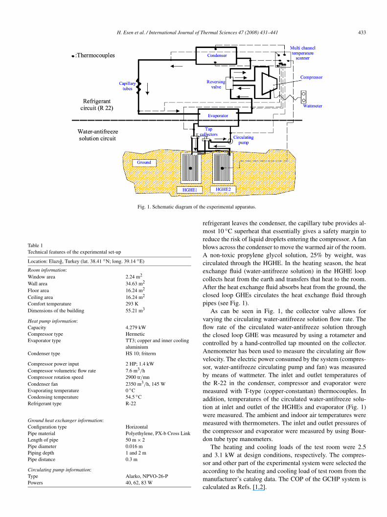
The schematic of the horizontal GCHP system constructedfor space heating is illustrated in Fig. 1. Table 1 summarizes themain components specification and characteristics of the GCHPsystem. The experimental set-up consists of three main compo-nents:

• Horizontal ground heat exchanger (HGHE),• heat pump unit equipment,• auxiliary equipment.

There have been two GHEs installed at the University of Fi-rat. Each consists of a high density polyethylene tube, 0.016 mdiameter. The HGHE1 and HGHE2 are made as a single passstraight tube, buried at the depth of 1 and 2 m. The heat ex-changers were been buried in the native ground. To allow formeasurement of the circulating water-antifreeze solution andground temperature a number of T-type thermocouples were in-stalled. The pipe–ground interface temperature is measured ina similar fashion to the water-antifreeze solution-temperaturemeasurement; except that thermal insulation is not used heresince the thermocouple should have good contact with both thepipe and the ground.

The heat transfer from Earth to the heat pump or fromthe heat pump to Earth is maintained with the fluid or water-antifreeze solution circulated through the HGHEs. The fluidtransfers its heat to refrigerant fluid in the evaporator (the water-antifreeze solution to refrigerant heat exchanger). The refriger-ant, which flows through other closed loop in the heat pump,evaporates by absorbing heat from the water-antifreeze solutioncirculated through the evaporator and then enters the hermeticcompressor. The refrigerant is compressed by the compressorand then enters the condenser, where it condenses. After the

H. Esen et al. / International Journal of Thermal Sciences 47 (2008) 431–441 433

Fig. 1. Schematic diagram of the experimental apparatus.

Table 1Technical features of the experimental set-up

Location: Elazıg, Turkey (lat. 38.41 ◦N; long. 39.14 ◦E)

Room information:Window area 2.24 m2

Wall area 34.63 m2

Floor area 16.24 m2

Ceiling area 16.24 m2

Comfort temperature 293 KDimensions of the building 55.21 m3

Heat pump information:Capacity 4.279 kWCompressor type HermeticEvaporator type TT3; copper and inner cooling

aluminiumCondenser type HS 10; friterm

Compressor power input 2 HP; 1.4 kWCompressor volumetric flow rate 7.6 m3/hCompressor rotation speed 2900 tr/mnCondenser fan 2350 m3/h, 145 WEvaporating temperature 0 ◦CCondensing temperature 54.5 ◦CRefrigerant type R-22

Ground heat exchanger information:Configuration type HorizontalPipe material Polyethylene, PX-b Cross LinkLength of pipe 50 m × 2Pipe diameter 0.016 mPiping depth 1 and 2 mPipe distance 0.3 m

Circulating pump information:Type Alarko, NPVO-26-PPowers 40, 62, 83 W

refrigerant leaves the condenser, the capillary tube provides al-most 10 ◦C superheat that essentially gives a safety margin toreduce the risk of liquid droplets entering the compressor. A fanblows across the condenser to move the warmed air of the room.A non-toxic propylene glycol solution, 25% by weight, wascirculated through the HGHE. In the heating season, the heatexchange fluid (water-antifreeze solution) in the HGHE loopcollects heat from the earth and transfers that heat to the room.After the heat exchange fluid absorbs heat from the ground, theclosed loop GHEs circulates the heat exchange fluid throughpipes (see Fig. 1).

As can be seen in Fig. 1, the collector valve allows forvarying the circulating water-antifreeze solution flow rate. Theflow rate of the circulated water-antifreeze solution throughthe closed loop GHE was measured by using a rotameter andcontrolled by a hand-controlled tap mounted on the collector.Anemometer has been used to measure the circulating air flowvelocity. The electric power consumed by the system (compres-sor, water-antifreeze circulating pump and fan) was measuredby means of wattmeter. The inlet and outlet temperatures ofthe R-22 in the condenser, compressor and evaporator weremeasured with T-type (copper-constantan) thermocouples. Inaddition, temperatures of the circulated water-antifreeze solu-tion at inlet and outlet of the HGHEs and evaporator (Fig. 1)were measured. The ambient and indoor air temperatures weremeasured with thermometers. The inlet and outlet pressures ofthe compressor and evaporator were measured by using Bour-don tube type manometers.

The heating and cooling loads of the test room were 2.5and 3.1 kW at design conditions, respectively. The compres-sor and other part of the experimental system were selected theaccording to the heating and cooling load of test room from themanufacturer’s catalog data. The COP of the GCHP system iscalculated as Refs. [1,2].

434 H. Esen et al. / International Journal of Thermal Sciences 47 (2008) 431–441

3. Experimental analysis and uncertainty

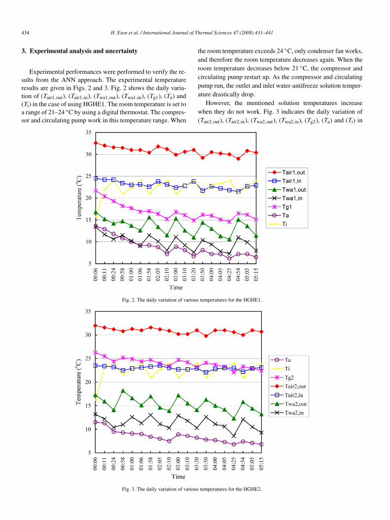
Experimental performances were performed to verify the re-sults from the ANN approach. The experimental temperatureresults are given in Figs. 2 and 3. Fig. 2 shows the daily varia-tion of (Tair1,out), (Tair1,in), (Twa1,out), (Twa1,in), (Tg1), (Ta) and(Ti) in the case of using HGHE1. The room temperature is set toa range of 21–24 ◦C by using a digital thermostat. The compres-sor and circulating pump work in this temperature range. When

the room temperature exceeds 24 ◦C, only condenser fan works,and therefore the room temperature decreases again. When theroom temperature decreases below 21 ◦C, the compressor andcirculating pump restart up. As the compressor and circulatingpump run, the outlet and inlet water-antifreeze solution temper-ature drastically drop.

However, the mentioned solution temperatures increasewhen they do not work. Fig. 3 indicates the daily variation of(Tair2,out), (Tair2,in), (Twa2,out), (Twa2,in), (Tg2), (Ta) and (Ti) in

Fig. 2. The daily variation of various temperatures for the HGHE1.

Fig. 3. The daily variation of various temperatures for the HGHE2.

H. Esen et al. / International Journal of Thermal Sciences 47 (2008) 431–441 435

the case of using HGHE2. It can be seen from Fig. 3 that thetrends in (Tair2,out), (Tair2,in), (Twa2,out), (Twa2,in), (Tg2), (Ta)and (Ti) are similar to those given in Fig. 2.

The COP of the GCHP system was calculated by Refs. [1,2].The COP increases with increasing the buried depth of HGHE.Thus, the much more proper HGHEs design gives higher en-hancement rates for COP.

An important issue is the accuracy of the measured data aswell as the results obtained by experimental studies. Uncer-tainty is a measure of the “goodness” of a result. Without sucha measure, it is impossible to judge the fitness of the value as abasis for making decisions relating to health, safety, commerceor scientific excellence.

The result R is a given function in terms of the indepen-dent variables. Let wR be the uncertainty in the result andw1,w2, . . . ,wn be the uncertainties in the independent vari-ables. The result R is a given function of the independent vari-ables x1, x2, x3, . . . , xn. If the uncertainties in the independentvariables are all given with same odds, then uncertainty in theresult having these odds is calculated by [8]

wR =[(

∂R

∂x1w1

)2

+(

∂R

∂x2w2

)2

+ · · · +(

∂R

∂xn

wn

)2]1/2

(1)

It is important that all uncertainties used in Eq. (1) can be eval-uated at the same confidence level. The uncertainty estimates inthe COP can be calculated from Eq. (1) as

wCOP =[(

∂COP

∂ρairwρair

)2

+(

∂COP

∂VairwVair

)2

+(

∂COP

∂Cp,airwcp,air

)2

+(

∂COP

∂Tair,outwTair,out

)2

+(

∂COP

∂Tair,inwTair,in

)2

+(

∂COP

∂WcwWC

)2

+(

∂COP

∂WpwWp

)2

+(

∂COP

∂WcfwWcf

)2]1/2

(2)

The total uncertainties of the measurements are estimated tobe ±2.89% for the water-antifreeze temperatures and refrig-erant temperatures, ±2.75% for pressures, ±4.35% for powerinputs to the compressor, condenser fan and circulating pump,and ±3.00% for electric currents. Uncertainty in reading valuesof the table is assumed to be ±0.20%. The overall uncertaintyfor COP calculations was found to be 3.94 % for the R-22 test.The uncertainty of COP is small enough.

4. Artificial neural networks (ANNs)

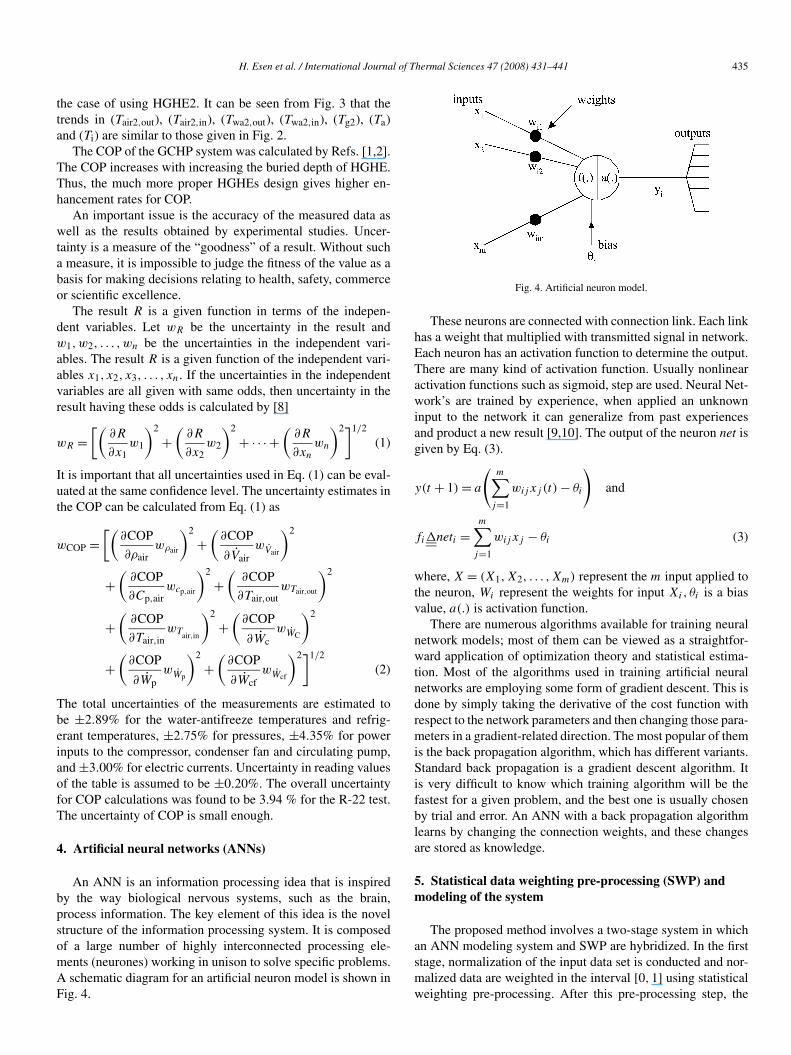
An ANN is an information processing idea that is inspiredby the way biological nervous systems, such as the brain,process information. The key element of this idea is the novelstructure of the information processing system. It is composedof a large number of highly interconnected processing ele-ments (neurones) working in unison to solve specific problems.A schematic diagram for an artificial neuron model is shown inFig. 4.

Fig. 4. Artificial neuron model.

These neurons are connected with connection link. Each linkhas a weight that multiplied with transmitted signal in network.Each neuron has an activation function to determine the output.There are many kind of activation function. Usually nonlinearactivation functions such as sigmoid, step are used. Neural Net-work’s are trained by experience, when applied an unknowninput to the network it can generalize from past experiencesand product a new result [9,10]. The output of the neuron net isgiven by Eq. (3).

y(t + 1) = a

(m∑

j=1

wijxj (t) − θi

)and

fi�neti =m∑

j=1

wijxj − θi (3)

where, X = (X1,X2, . . . ,Xm) represent the m input applied tothe neuron, Wi represent the weights for input Xi, θi is a biasvalue, a(.) is activation function.

There are numerous algorithms available for training neuralnetwork models; most of them can be viewed as a straightfor-ward application of optimization theory and statistical estima-tion. Most of the algorithms used in training artificial neuralnetworks are employing some form of gradient descent. This isdone by simply taking the derivative of the cost function withrespect to the network parameters and then changing those para-meters in a gradient-related direction. The most popular of themis the back propagation algorithm, which has different variants.Standard back propagation is a gradient descent algorithm. Itis very difficult to know which training algorithm will be thefastest for a given problem, and the best one is usually chosenby trial and error. An ANN with a back propagation algorithmlearns by changing the connection weights, and these changesare stored as knowledge.

5. Statistical data weighting pre-processing (SWP) andmodeling of the system

The proposed method involves a two-stage system in whichan ANN modeling system and SWP are hybridized. In the firststage, normalization of the input data set is conducted and nor-malized data are weighted in the interval [0,1] using statisticalweighting pre-processing. After this pre-processing step, the

436 H. Esen et al. / International Journal of Thermal Sciences 47 (2008) 431–441

Fig. 5. Proposed model block diagram.

weighted data set was presented to the main modeling unit. Thesecond stage uses ANN to model weighted data.

The procedure of the proposed statistical weighed pre-processing stage is defined as follows;

Assume that the data set which is going to be used for mod-eling the GCHP system is composed of L × N matrix. WhereL indicates the number of input variables and N indicates thenumber of samples per variable. The algorithm of the proposedstatistical weighting pre-processing system is given as follow-ing:

(1) Determine the number of the input variables (L)(2) For each input variable (i = 1,2,3, . . . ,L), do:

(2.1) Calculate the standard deviation of the input vari-able i:

std(Xi) =√√√√ 1

N

N∑k=1

(Xk,i − μ(Xi)

)2 (4)

where μ(Xi) is the mean value of the ith input vari-able for N samples and can be calculated as follow-ing:

μ(Xi) = 1

N

N∑k=1

xk (5)

(2.2) Calculate the weight for ith input variable as given:

wi = μ(Xi)

std(Xi)(6)

(3) Update the input variables with the calculated wi weights.

new(Xi) = wi ∗ old(Xi) (7)

In the statistical weighting pre-processing, the training samplesare used for determining the effect of each input variable tothe system modeling procedure. The variable which has moreinfluence on the system modeling will get the more weightsthan the other input variables. Thus, each variable takes newvalues according to its old values. Moreover, it is assumed thatthe input variable which has less deviation for N samples isthe best for modeling the examined system. But, if a variable

changes abruptly, that variable is assumed to be less importantin using the modeling procedure.

There are many types of ANN architectures in the literature;however, multi-layer feed-forward neural network is the mostwidely used for prediction. A multi-layer feed-forward neuralnetwork typically has an input layer, an output layer, and one ormore hidden layers [3]. In multi-layer feed-forward networks,neurons are arranged in layers and there is a connection amongthe neurons of other layers. The input signals are applied to theinput layer, the output layer contributes to the output signal di-rectly. Other layers between input and output layers are calledhidden layers. Input signals are propagated in gradually mod-ified form in the forward direction, finally reaching the outputlayer [11].

In this study, the model has five input variables and oneoutput variable. Air temperature entering the condenser unit(Tair,in), air temperature leaving the condenser unit (Tair,out),water-antifreeze solution entering the HGHEs (Twa,in), water-antifreeze solution leaving the HGHEs (Twa,out) and groundtemperatures at 1 and 2 meters (Tg1 and Tg2) constitutes theinput variables of the model. The COP of the system is the out-put variable of the ANN model. The inputs of the model arenormalized in the (0,1) range with the SWP. The output valuesare not normalized.

The block diagram of the proposed model is given in Fig. 5.As can be seen from the block diagram; ANN model is adjusted,or trained, so that a particular input leads to a specific target out-put. Here, the ANN model is adjusted, based on a comparisonof the output and the target, until the model output matches thetarget. Typically, many such input/target output pairs are usedto train a model.

The training parameters and the structure of the ANN usedin this study are as shown in Table 2. These were selected forthe best performance, after several different experiments, suchas the number of hidden layers, the size of the hidden layers,value of learning rate, and type of the activation functions.

6. Results and discussion

In order to indicate the efficiency of the proposed SWP andANN structure for modeling purposes, a computer program was

H. Esen et al. / International Journal of Thermal Sciences 47 (2008) 431–441 437

Table 2ANN architecture and training parameters

Architecture

The number of layers 3The number of neuron on the layers Input: 5

Hidden: 5, 6, 7, 8, 9, 10, 11, 12, 13, 14and 15Output: 1

The initial weights and biases RandomActivation functions Tangent Sigmoid

Training parametersLearning rule Scaled Conjugate Gradient (SCG)Learning rate 0.8Mean-squared error 1e−07

performed under MATLAB (version 5.3. The MathWorks Inc.,USA) environment using the neural network toolbox.

The optimal model parameters such as different training al-gorithms, initial weights and activation function of the ANNwere investigated elsewhere [6,10] and out of scope of thispaper. Here, we only investigated the effect of the SWP ofthe input data set on performance when modeling with ANN.Moreover, a variable number of neurons (from 5 to 15) wereused in the hidden layer to observe as any performance im-provement can be obtained with the proposed modeling sys-tem. Thus, we constructed the ANN model with the parameterswhich are given in Table 2. The data set was divided into twoseparate data sets randomly—the training data set and the test-ing data set. The training data set was used to train the ANNmodel, whereas the testing data set was used to verify the accu-racy and the effectiveness of the trained ANN model for GCHPsystem (for HGHE1 and HGHE2). The adequate functioning ofthe ANN depends on the sizes of the training set and test set.The data set for the COP of GCHP system (for HGHE1 andHGHE2) available included 38 data patterns. From these, 25data patterns were used for training the ANN, and the remain-ing 13 patterns were used as the test data set for trained ANNmodel.

Model validation is the process by which the input vectorsfrom input/output data sets on which the ANN was not trained,are presented to the trained model, to see how well the trainedmodel predicts the corresponding data set output values. Somestatistical methods, such as the root-mean squared (RMS), thecoefficient of multiple determinations (R2) and the coefficientof variation (cov) may be used to compare predicted and actualvalues for model validation.

The error can be estimated by the RMS, defined as [10,12]:

RMS =√∑n

m=1(ypre,m − tmea,m)2

n(8)

In addition, the coefficient of multiple determinations (R2)and the coefficient of variation (cov) in percent are defined asfollows:

R2 = 1 −∑n

m=1(ypre,m − tmea,m)2∑n(t )2

(9)

m=1 mea,m

Table 3Statistical values of COP for ANN

Algorithm-neurons RMS cov R2

SCG5 0.472323 14.521747 0.979375SCG6 0.074953 2.220088 0.999871SCG7 0.217507 6.327536 0.996017SCG8 0.452977 11.827146 0.986067SCG9 0.111438 3.170915 0.998996SCG10 0.366284 10.730821 0.988589SCG11 0.171011 4.747563 0.997748SCG12 0.255057 7.544056 0.994344SCG13 0.163817 4.681177 0.997812SCG14 0.148872 4.208714 0.998229SCG15 0.123272 3.495283 0.998779

Fig. 6. Variation of mean-square error with training epochs for SCG6 topology.(For interpretation of the references to color in this figure, the reader is referredto the web version of this article.)

cov = RMS

|tmea,m|100 (10)

where n is the number of data patterns in the independent dataset, ypre,m indicates the predicted, tmea,m is the measured valueof one data point m, and tmea,m is the mean value of all mea-sured data points.

The computer simulations are carried out as the followingmanner; first; ANN topologies with various number of hiddenlayer neurons are trained without SWP normalized inputs. Butfor the sake of justice, we have normalized the ANN inputsby dividing the each sample with a constant value. Therefore,the input vector of the ANN was normalized to (0,1) range.The prediction results of the ANN models are given in Ta-ble 3. The training performance of the ANN (SCG6 topology)is given in Fig. 6 where the variation of mean-square error withtraining epochs is illustrated. Fig. 7 also shows the compari-son of calculated and ANN predicted COP values of GCHPsystem for SCG6 and the model error for each test sampleis shown in Fig. 8. Second, the ANN topologies with variousnumber of hidden layer neurons are trained with the statisticalweighting pre-processed inputs. The related test results (RMS,

438 H. Esen et al. / International Journal of Thermal Sciences 47 (2008) 431–441

Fig. 7. Comparison of calculated and ANN predicted values of GCHP systemCOP for SCG6.

Fig. 8. Error for each sample for SCG6.

cov and R2) are represented in Table 4. The decrease of thetraining performance during the training process of SWP-SCG6topology is shown in Fig. 9. In this figure the variation of mean-square error with training epochs is given. The input variablesagainst to the output variables of SWP-SCG6 topology for thetest data set are also shown in Fig. 10. The errors of the SWP-SCG6 model predictions for each test sample are also given inFig. 11.

One observes from both cases (ANN with SWP and onlyANN) by decreasing the number of hidden neurons the trainingaccuracy improves, as indicated by the smaller RMS and covvalues and R2-values approaching 1 (Tables 3 and 4). On theother hand, beyond a certain point the errors obtained begin toincrease together with the complexity of the ANN as the largerthe number of hidden neurons the more complex the networkis. So, the convergence to the target error rate (1e−007) takes

Fig. 9. Variation of mean-square error with training epochs for SWP-SCG6topology. (For interpretation of the references to color in this figure, the readeris referred to the web version of this article.)

Fig. 10. Comparison of calculated and predicted COP values for SWP-SCG6.

more iteration. This situation is very time consuming. Fromthe statistical data presented in Tables 3 and 4, for COP val-ues SWP-SCG6 algorithm with six neurons in the hidden layerappeared to be most optimal topology. This topology gained0.002665 RMS value, 0.076557 cov value and, 0.999999 R2

value, respectively. These values are really promising. The restof the SWP based ANN modeling results are also promising.The R2 value of each topology is 0.9999 and RMS and covvalues are considerably small. It is observed during the sev-eral runs of the computer simulation that the convergence ofthe SWP-ANN takes more iteration. But the average predictionerror is quite small. This situation can be seen in Fig. 11.

The statistical results of the first stage of the computer sim-ulation are given in Table 4. As it is aforementioned, this stageinvolves the usage of only ANN structure for modeling pur-poses. The related prediction results and structural information

H. Esen et al. / International Journal of Thermal Sciences 47 (2008) 431–441 439

Fig. 11. Error for each sample for SWP-SCG6.

Table 4Statistical values of COP for ANN with SWP normalization

Algorithm-neurons RMS cov R2

SWP-SCG5 0.004989 0.143290 0.999997SWP-SCG6 0.002665 0.076557 0.999999SWP-SCG7 0.004903 0.140958 0.999998SWP-SCG8 0.006267 0.179854 0.999996SWP-SCG9 0.002734 0.078810 0.999999SWP-SCG10 0.002835 0.081417 0.999999SWP-SCG11 0.003513 0.100882 0.999998SWP-SCG12 0.005919 0.169903 0.999997SWP-SCG13 0.007908 0.227402 0.999994SWP-SCG14 0.013958 0.175948 0.999927SWP-SCG15 0.013665 0.391664 0.999984

Fig. 12. Comparison of calculated and predicted COP values for SWP-SCG6(the first part of the data set).

Fig. 13. Comparison of calculated and predicted COP values for SWP-SCG6(the second part of the data set).

of the ANN are given in subsequent graphics. One observesfrom Table 3, where this table gave us the statistical validationof the proposed modeling, the most appropriate ANN topol-ogy is SCG6. 0.074953 RMS value, 2.220088 cov value and0.999871 R2 value is obtained for test patterns. The rest of theresults are obtained for the related ANN structures. These re-sults are not promising when compared with the results whichwere obtained with SWP-ANN structure. The convergence ofthese structures is not taken more iteration. The running time ofthe computer simulation of these structures is less than SWP-ANN structure.

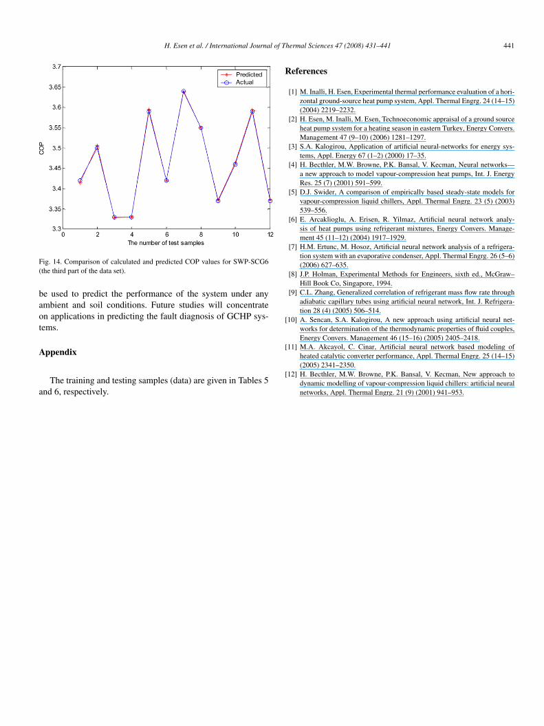
Moreover, the efficiency of the proposed method was demon-strated by using the 3-fold cross validation test. In 3-fold crossvalidation dataset is randomly split into three exclusive sub-sets (X1, . . . ,X3) of approximately equal size and the holdoutmethod is repeated 3 times. These subsets contain 13, 13 and12 samples (13 + 13 + 12 = 38) respectively. At each time, oneof the three subsets is used as the test set and the other two sub-sets are put together to form a training set. The advantage ofthis method is that it is not important how the data is divided.Every data point appears in a test set only once, and appears in atraining set 2 times. Therefore, the verification of the efficiencyof the proposed method against to the over-learning problemshould be demonstrated. The 3-fold cross validation test resultswere shown in Figs. 12, 13 and 14, respectively. The first subsetof the cross validation test was shown in Fig. 12 and the secondpart of the data set and the predicted COP values were given inFig. 13 and finally the last part of the data set was already givenin Fig. 14.

7. Conclusions

The objective of this work is to improve the performance ofan ANN with a SWP method to learn to predict GCHP sys-tems with the minimum data set. To evaluate the effectivenessof our proposal (SWP-ANN), a computer simulation is devel-

440 H. Esen et al. / International Journal of Thermal Sciences 47 (2008) 431–441

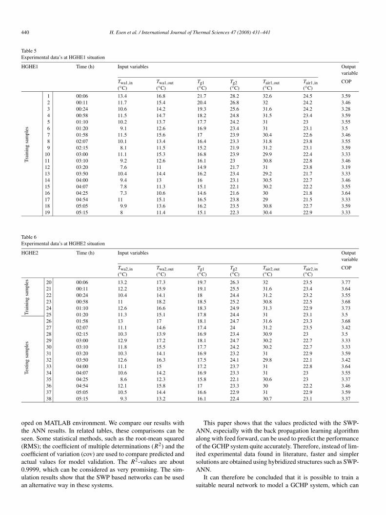
Table 5Experimental data’s at HGHE1 situation

HGHE1 Time (h) Input variables Outputvariable

Twa1,in Twa1,out Tg1 Tg2 Tair1,out Tair1,in COP(◦C) (◦C) (◦C) (◦C) (◦C) (◦C)

Tra

inin

gsa

mpl

es

1 00:06 13.4 16.8 21.7 28.2 32.6 24.5 3.592 00:11 11.7 15.4 20.4 26.8 32 24.2 3.463 00:24 10.6 14.2 19.3 25.6 31.6 24.2 3.284 00:58 11.5 14.7 18.2 24.8 31.5 23.4 3.595 01:10 10.2 13.7 17.7 24.2 31 23 3.556 01:20 9.1 12.6 16.9 23.4 31 23.1 3.57 01:58 11.5 15.6 17 23.9 30.4 22.6 3.468 02:07 10.1 13.4 16.4 23.3 31.8 23.8 3.559 02:15 8.1 11.5 15.2 21.9 31.2 23.1 3.59

10 03:00 11.1 15.3 16.8 23.9 29.9 22.4 3.3311 03:10 9.2 12.6 16.1 23 30.8 22.8 3.4612 03:20 7.6 11 14.9 21.7 31 23.8 3.1913 03:50 10.4 14.4 16.2 23.4 29.2 21.7 3.3314 04:00 9.4 13 16 23.1 30.5 22.7 3.4615 04:07 7.8 11.3 15.1 22.1 30.2 22.2 3.5516 04:25 7.3 10.6 14.6 21.6 30 21.8 3.6417 04:54 11 15.1 16.5 23.8 29 21.5 3.3318 05:05 9.9 13.6 16.2 23.5 30.8 22.7 3.5919 05:15 8 11.4 15.1 22.3 30.4 22.9 3.33

Table 6Experimental data’s at HGHE2 situation

HGHE2 Time (h) Input variables Outputvariable

Twa2,in Twa2,out Tg1 Tg2 Tair2,out Tair2,in COP(◦C) (◦C) (◦C) (◦C) (◦C) (◦C)

20 00:06 13.2 17.3 19.7 26.3 32 23.5 3.77

Tra

inin

gsa

mpl

es

21 00:11 12.2 15.9 19.1 25.5 31.6 23.4 3.6422 00:24 10.4 14.1 18 24.4 31.2 23.2 3.5523 00:58 11 18.2 18.5 25.2 30.8 22.5 3.6824 01:10 12.6 16.6 18.3 24.9 31.3 22.9 3.7325 01:20 11.3 15.1 17.8 24.4 31 23.1 3.5

Test

ing

sam

ples

26 01:58 13 17 18.1 24.7 31.6 23.3 3.6827 02:07 11.1 14.6 17.4 24 31.2 23.5 3.4228 02:15 10.3 13.9 16.9 23.4 30.9 23 3.529 03:00 12.9 17.2 18.1 24.7 30.2 22.7 3.3330 03:10 11.8 15.5 17.7 24.2 30.2 22.7 3.3331 03:20 10.3 14.1 16.9 23.2 31 22.9 3.5932 03:50 12.6 16.3 17.5 24.1 29.8 22.1 3.4233 04:00 11.1 15 17.2 23.7 31 22.8 3.6434 04:07 10.6 14.2 16.9 23.3 31 23 3.5535 04:25 8.6 12.3 15.8 22.1 30.6 23 3.3736 04:54 12.1 15.8 17 23.3 30 22.2 3.4637 05:05 10.5 14.4 16.6 22.9 31 22.9 3.5938 05:15 9.3 13.2 16.1 22.4 30.7 23.1 3.37

oped on MATLAB environment. We compare our results withthe ANN results. In related tables, these comparisons can beseen. Some statistical methods, such as the root-mean squared(RMS); the coefficient of multiple determinations (R2) and thecoefficient of variation (cov) are used to compare predicted andactual values for model validation. The R2-values are about0.9999, which can be considered as very promising. The sim-ulation results show that the SWP based networks can be usedan alternative way in these systems.

This paper shows that the values predicted with the SWP-ANN, especially with the back propagation learning algorithmalong with feed forward, can be used to predict the performanceof the GCHP system quite accurately. Therefore, instead of lim-ited experimental data found in literature, faster and simplersolutions are obtained using hybridized structures such as SWP-ANN.

It can therefore be concluded that it is possible to train asuitable neural network to model a GCHP system, which can

H. Esen et al. / International Journal of Thermal Sciences 47 (2008) 431–441 441

Fig. 14. Comparison of calculated and predicted COP values for SWP-SCG6(the third part of the data set).

be used to predict the performance of the system under anyambient and soil conditions. Future studies will concentrateon applications in predicting the fault diagnosis of GCHP sys-tems.

Appendix

The training and testing samples (data) are given in Tables 5and 6, respectively.

References

[1] M. Inalli, H. Esen, Experimental thermal performance evaluation of a hori-zontal ground-source heat pump system, Appl. Thermal Engrg. 24 (14–15)(2004) 2219–2232.

[2] H. Esen, M. Inalli, M. Esen, Technoeconomic appraisal of a ground sourceheat pump system for a heating season in eastern Turkey, Energy Convers.Management 47 (9–10) (2006) 1281–1297.

[3] S.A. Kalogirou, Application of artificial neural-networks for energy sys-tems, Appl. Energy 67 (1–2) (2000) 17–35.

[4] H. Becthler, M.W. Browne, P.K. Bansal, V. Kecman, Neural networks—a new approach to model vapour-compression heat pumps, Int. J. EnergyRes. 25 (7) (2001) 591–599.

[5] D.J. Swider, A comparison of empirically based steady-state models forvapour-compression liquid chillers, Appl. Thermal Engrg. 23 (5) (2003)539–556.

[6] E. Arcaklioglu, A. Erisen, R. Yilmaz, Artificial neural network analy-sis of heat pumps using refrigerant mixtures, Energy Convers. Manage-ment 45 (11–12) (2004) 1917–1929.

[7] H.M. Ertunc, M. Hosoz, Artificial neural network analysis of a refrigera-tion system with an evaporative condenser, Appl. Thermal Engrg. 26 (5–6)(2006) 627–635.

[8] J.P. Holman, Experimental Methods for Engineers, sixth ed., McGraw–Hill Book Co, Singapore, 1994.

[9] C.L. Zhang, Generalized correlation of refrigerant mass flow rate throughadiabatic capillary tubes using artificial neural network, Int. J. Refrigera-tion 28 (4) (2005) 506–514.

[10] A. Sencan, S.A. Kalogirou, A new approach using artificial neural net-works for determination of the thermodynamic properties of fluid couples,Energy Convers. Management 46 (15–16) (2005) 2405–2418.

[11] M.A. Akcayol, C. Cinar, Artificial neural network based modeling ofheated catalytic converter performance, Appl. Thermal Engrg. 25 (14–15)(2005) 2341–2350.

[12] H. Becthler, M.W. Browne, P.K. Bansal, V. Kecman, New approach todynamic modelling of vapour-compression liquid chillers: artificial neuralnetworks, Appl. Thermal Engrg. 21 (9) (2001) 941–953.