Exploration of cellular reaction systems

Exploration of cellular reaction systemsMarkus Kirkilionis*Submitted: 10th April 2009; Received (in revised form): 11th July 2009

AbstractWe discuss and review different ways to map cellular components and their temporal interaction with other suchcomponents to different non-spatially explicit mathematical models. The essential choices made in the literatureare between discrete and continuous state spaces, between rule and event-based state updates and between deter-ministic and stochastic series of such updates.The temporal modelling of cellular regulatory networks (dynamic net-work theory) is compared with static network approaches in two first introductory sections on general networkmodelling. We concentrate next on deterministic rate-based dynamic regulatory networks and their derivation.In the derivation, we include methods from multiscale analysis and also look at structured large particles, herecalled macromolecular machines. It is clear that mass-action systems and their derivatives, i.e. networks based onenzyme kinetics, play the most dominant role in the literature. The tools to analyse cellular reaction networks arewithout doubt most complete for mass-action systems. We devote a long section at the end of the review tomake a comprehensive review of related tools and mathematical methods. The emphasis is to show how cellularreaction networks can be analysed with the help of different associated graphs and the dissection into modules,i.e. sub-networks.

Keywords: cellular reaction systems; modelling; graph theory; master equations; continuum limit; qualitative behaviour

SYSTEM IDENTIFICATION:MAPPING CELLULARREACTIONSYSTEMSTOGRAPHSWe start this review with two small sections (this

section and ‘static and dynamic network concepts’

section) on general network modelling and system

identification. This is necessary because network

theory is rapidly expanding, and we have to fix

some ideas and concepts that are sometimes called

differently or stay undefined in some areas. We then

start the discussion of dynamic cellular regulatory

networks in ‘stochastic versus deterministic reaction

networks’ section.

As most ‘camps’ inside the philosophy of science

would agree, experimental data can only be under-

stood in the presence of concepts that allow their

interpretation in a context. These concepts them-

selves are often called ‘a priori knowledge’ since

Kant introduced this notion into the philosophical

discussion. But they are surely in praxis just

something that might have been established on the

basis of experimental evidence before the actual data

were taken, or these concepts are so basic that they

simply establish a rational choice between several

logical possibilities. Such a concept in the context

of cellular reaction systems is surely the graph. The

graph is a fundamental mathematical object consist-

ing of two sets, G¼ (V,E ), the vertex and the edge

sets. In our context, the vertices will represent the

system components and the edges the interaction between

them. In the following we describe how to system-

atically introduce graphs as tools to translate a

time-dependent cell biology situation where space

can be neglected into an either stochastic or deter-

ministic dynamical system. At the end of the process,

there appears a mathematical model that describes

how the system’s states (attached in an abstraction

process to several components like molecules, mem-

branes, etc. and linked together inside a network)

change in time. Later we will also go the reverse

MarkusKirkilionis was studying mathematics and biology at the University of Heidelberg under the supervision of Willi Jager. He is

interested in applying mathematics to cell biology and ecology, with applications currently expanding through his research in complex

systems.

*Mathematics Institute, University of Warwick, Coventry CV4 7AL, UK. Tel: þ44 24765 24849; Fax: þ44 24765 24182;

E-mail: [email protected]

BRIEFINGS IN BIOINFORMATICS. VOL 11. NO 1. 153^178 doi:10.1093/bib/bbp062

� The Author 2010. Published by Oxford University Press. For Permissions, please email: [email protected]

by guest on August 10, 2016

http://bib.oxfordjournals.org/D

ownloaded from

http://bib.oxfordjournals.org/

way, and attach graphs to already established types of

reaction networks in order to analyse their qualitative

behaviour.

Interacting componentsThe natural situation to analyse the state of a cell, still

the most central entity in biology, is the first to iden-

tify components that, due to their presence, establish

the basis of cellular function, and secondly to study

the components’ interaction and transformations that

will cause the cell to change and possibly adapt to

signals stemming from outside. Even the first step in

this blueprint concept is presently still cumbersome,

in some cases even impossible. Why should this be

the case? Typical system components for cellular sys-

tems, frequently used in bioinformatics and systems

biology, are molecular species, even different variants

or conformations of the same molecule, molecular

complexes or slightly more abstract entities such as

genes. This list already shows that cellular system

components can be chosen as being embedded into

and acting on different spatial and temporal scales.

This will make it often necessary to introduce a

mathematical multiscale analysis in order to under-

stand how system components influence or interact

with each other. We will come back to such multi-

scale ideas later in this review.

If, for example, a specific signalling pathway is

under investigation, most often many of the different

molecules involved are unknown, or there is a high

probability that some yet unknown molecules will

have a role in this pathway, at least under slightly

changed experimental conditions. It is therefore no

wonder that different ways of experimental compo-

nent detection, typically high-throughput methods

and respective tools from bioinformatics, are pres-

ently core techniques to establish biological knowl-

edge. These ‘system component detection’ methods

are essential for biological research, and there is much

overlap with the methods discussed in this review.

Possibilities include the detection of missing compo-

nents by measured dynamical anomalies, very much

analogous to the detection of new planets disturbing

the orbits of known ones. But typically biological

system component detection by large-scale screening

is for good reasons a static (non-temporal) procedure.

The yet unclassified newly detected objects are

clustered into groups according to some detected

function and its disruption or disturbance, for

example realized in mutagenesis experiments [1, 2].

Sometimes detection and (non-temporal) functional

characterization of components can be automized as

described in King et al. [3]. In the following we will

not discuss such methods, as our goal is to focus on

dynamical models predicting the temporally varying

states of previously identified cellular components.

In other words we will assume that the system com-

ponents are already well characterized and proceed

to analyse their temporal state changes.

Bioinformatics has traditionally its biggest suc-

cesses in the component detection area. One just

needs to think about the detection of genes inside

DNA strings. All such algorithms are based on dis-

crete data, but as we will explore reaction systems

there appear additional challenges in the sense that

the use of a combination of discrete and continuous

data objects is needed.

InteractionAfter the choice of the system components such as

(a certain family of ) proteins, the type of interaction

between them needs to be established. It is very

important to note that both the choice of system

components as well as the type of interaction will

depend on the experimental set up. In many, if not

most cases, the experimental design and technology

will be available before any modelling and analysis,

and therefore before the system identification step. In

general, theory and experiment have to adapt to each

other, and this will be done in a recursive way while

stepping through a guiding diagram like Figure 1. In

a first step inside the identification of interaction a funda-

mental test has to performed: Is the interaction sym-

metric or non-symmetric? What we describe here is

much the same as to translate a typical cell biology

diagram into a mathematical model. We first design a

graph by representing the system components as ver-

tices and find their relations (interactions), which is

already describing the system mathematically. The

interaction is symmetric if there exists a binary rela-

tion between the components. It is non-symmetric

if a component is influencing another component,

but not necessarily the other way round. The most

obvious symmetric relationship in this context is

‘component A binds to component B’, which is a

common property of (bio-)molecules. This leads to a

description of the system as an undirected graph. An

example for a non-symmetric relation is ‘component

A influences B’, or ‘component A modifies compo-

nent B’. An example is post-translational modifica-

tion or when component A produces the substrate of

component B in a metabolic context. On a more

154 Kirkilionis by guest on A

ugust 10, 2016http://bib.oxfordjournals.org/

Dow

nloaded from


abstract level, this directed relation holds when a gene

A is ‘upstream’ of gene B. The system now is repre-

sented as a, directed graph with arrows as edges. Once

a static graph topology has been identified, we can

investigate its properties in terms of network con-

nectivity, looking at scale-free or exponential net-

work architectures (see the classical papers [7, 8]).

In this review, however, we will go a step further

and as stated before will be primarily interested in

temporal dynamics defined on networks. It will turn

out that the (static) network architecture or topology

is important, but that it cannot for good reasons

determine all the possible qualitative temporal beha-

viour of the network. This review focuses on some

situations where such a close link between architec-

ture (meaning the set of possible interactions

between system components) and the system’s tem-

poral behaviour can indeed be made.

STATICANDDYNAMIC NETWORKCONCEPTSThe next step is, therefore, to introduce a (temporal)

process, i.e. modelling a changing link structure over

time (varying network topology) and/or the states

attached to the nodes representing a quantity or

quality measured in some experimental set up. This

step, i.e. introducing a (stochastic) process acting on a

newly introduced state space structure, will be called

process identification in the following, see the next layer

in Figure 1. If—based on experimental evidence—

the network structure needs to vary temporarily,

and/or the number of components (this means

either the set E or in addition the set V of the

graph G¼G(V,E ) is changing over time) is not

fixed, there need to be rules included into the

model how this process is uniquely defined. We

will discuss this case briefly with the help of pro-

tein–protein networks to explain this model possibil-

ity inside a cell biology context. But even if we go

back to a fixed network topology (edge distribution)

with a given fixed number of components (nodes or

vertices), in most experimental situations a state space

has to be attached to the components for conceptual

closure of the problem. This is illustrated in Figure 2.

Introducing such state spaces to the nodes will

then also make it necessary to define a temporal pro-

cess on the network, which updates or changes the

state of the nodes in time. This abstract description is

best understood in the context of molecular reaction

systems. In this case, the network components are

most often associated with the molecular species

themselves, and there are experimental data available

showing the changing number of these molecules in

a given volume of observation. This will be indeed

our generic case. Each node representing a molecular

species will have a non-negative number (either an

integer or a real number) attached, depending on

whether we describe molecular number or concen-

tration. Of course also other, for example, finite dis-

crete state spaces are possible. In the most extreme

case, only binary states occur that might describe

whether a gene is switched on or off. Such

Boolean networks have been introduced to describe

genetic interation by Kauffman [16].

FluxesBoth graph theory and articles on biological regula-

tory networks often speak of fluxes or flows running

through the network (the flow defined on the graph

is realized as weights attached to the edges). A most

famous related concept is the Kirchoff laws of electric

circuit theory, making a conservation statement for

fluxes at nodes that are branching points. We will

look at fluxes again in ‘Enzyme Kinetics’ Section.

Here we define the flux along a given edge of the

network as the weight attached to it. The change of

Figure 1: The different layers in the process of iden-tifying cellular reaction systems, mapping to a mathe-matical model and comparison with experimental data.

Cellular reaction systems 155 by guest on A


Dow

nloaded from


this weight will be described by the dynamical

system defined on the network.

Static network concepts as special casesWe have already introduced static graph descriptions

like trees produced by a clustering algorithm in the

context of component identification. Evolutionary

trees of descendence would also fall into this

category. In this new context of networks equipped

with state spaces and processes, the static network

becomes a special case of the dynamic network.

The processes and so-called initial conditions

(initial conditions are the states of the network at

the beginning of the experimental observation) can

be such that the states will be in a dynamic equilib-

rium. Often this is also related to the concept of

homoeostasis. To analyse equilibria is often the best

way of entry to understand dynamic networks. It is

therefore no wonder equilibrium concepts play a

dominant role in the bioinformatics literature.

Once equilibria are introduced for dynamic net-

works, a natural mathematical question arising is

about their stability, i.e. whether any initial condi-

tions ‘close’ to the equilibrium will converge in time

back towards this equilibrium. In other words, the

static networks are now embeded inside a dynamical

context, and such analysis of the system will be done

with the help of mathematical methods we associate

with a temporal layer of the problem (Figure 1).

Static and evolving network topologies,protein^protein networksVery often in cell biology and bioinformatics, the

analysis is restricted to one type of molecule, for

example, the important class of proteins. As there

are binding assays for proteins, a binary relation can

be defined as ‘Protein A is binding to protein B’.

A complete map of proteins identified in a cell can

be mapped to an undirected graph G¼ (V,E), with

V being the set of proteins, and E being the set of

links between proteins. Clearly, such a link always

exist whenever two proteins can bind to each other.

Again the situation is static, i.e. the proteins bind to

each other whenever they are present in the system,

which here is assumed to be at ‘all times’. Knowing

the protein binding property implies that we know

the experimental nature of the interaction in the

graph, something which was not necessary for the

previously introduced combinatorial studies (com-

ponent analysis) we mentioned. A classic paper on

protein–protein networks is Jcong et al. [4]. Due to

refined mass spectroscopy, the wole set and even the

number of proteins in a cell can be measured [5].

Such numbers can be mapped to weights attached

to the vertices of the protein–protein network, at

any given moment in time (Figure 2). If protein

evolution is modelled, the network topology must

be modelled to change on the respective evolution-

ary time scale (see, for example, [6]).

STOCHASTIC VERSUSDETERMINISTIC REACTIONNETWORKSIn the rest of this article we restrict ourselves to

systems with a fixed number of components and

non-varying interactions (links) between them.

Most scientists would agree that nature is inherently

stochastic at ‘microscopic’ scales, for example (but

not only) due to quantum mechanistic effects. This

is indeed the philosophy we will adopt. The deter-

minsitic types of reaction systems are much easier to

analyse, and in many cases they are more intuitive.

Perhaps this is the reason why the most dynamic

network models in cell biology use such determinis-

tic reaction systems. But on the other side, there

Figure 2: Weights are attached to the nodes that arerepresenting here molecular species (left). The weightsare interpreted as state spaces that allow to capturemolecular concentrations in a given volume of experi-mental observation. In this interpretation, the statespace would be the non-negative real numbers attachedto each vertex. In a later step of the modelling process,other weights are attached to the arrows (right). Thearrows capture the strength of influence of one nodeto another. In dynamical network models, the strengthwill be associated with the frequency of events (reac-tions) that occur and that change the state of the nodeto which the arrow is pointing to. It should be notedthat strength can have positive and negative sign incase the nodes have natural numbers (numbers of mol-ecules) or non-negative real numbers (concentrations)as state spaces.



Dow

nloaded from


are many situations where the understanding of sto-

chastic effects is essential. The determinsitic systems

should best be introduced as averages of the stochas-

tic systems and/or after particle numbers can be

assumed to be sufficiently large, such that stochastic

fluctuations due to small numbers of particles/inter-

actions can be neglected. Let us first assume that

the entities/components of the systems we like to

describe can be characterized by a set of molecular

species S, say s such species. The molecular species

themselves are assumed to have no structure. Two

different conformations of the same molecule would

therefore have to be modelled as two different spe-

cies (this can be problematic, as in principle both

numbers of the species would need to be guaranteed

to be the same inside the evolution for all times). For

most metabolic systems such an assumption is very

reasonable. We write S¼ {S1, . . . ,Ss}. At this stage

we can introduce the directed species graph Gs,

discussed as a modelling tool in Figure 2, where

the species are the vertex set V, and the edges/

arrows contained in E have to be determined from

an investigation how the number or concentration of

a species Si will influence the number/concentration

of species Sj. The species graph GS will later reappear

as the so-called interaction graph GI, but then will be

introduced as a graph that is assigned to an already

specified reaction network. This difference is very

important to note; in the first case we use the

graph as a first model sketch, in the second case we

have a working model and derive the graphs as asso-

ciated mathematical objects needed for model

analysis.

The different molecular species can now be com-

bined in different ways. Each single reaction can

change the number and composition of the different

molecules in the system. In this case, a single reaction

will be the basic event, and we need an event-driven

stochastic process describing the evolution of the

system. Next we assume there are r posssible

transformations of molecules into each other, also

including the possibility that molecules leave or

enter the system. We also assume that only integer

combinations of molecular species can be formed.

In this case we can write each event/reaction rj in

the form

�1jS1 þ � � � þ �sjSs ! �1jS1 þ � � � þ �sjSs, ð1Þ

with j¼ 1, . . . , r. The integer coefficients �ij and �ijrepresent the number of Si molecules participating

in j-th reaction at reactant and product stages, respec-

tively. The net amount of species Si produced or

consumed by the reaction is named as the stoichio-

metric coefficient and is defined by nij:¼�ij-�ij.The integer coefficients nij can be assembled inside

the so-called stoichiometric (s� r) matrix N. In the

chemical literature [10], the linear combinations

of species to the left and right of the reaction

vector are called complexes. They can be interpreted

as a higher level of system components building a

new graph with the complexes as nodes. We can

define a directed link between these nodes whenever

a reaction between them is defined. This directed

graph G will be called the reaction graph GR.

Clearly the number c of nodes of GR is smaller or

equal to 2r. With respect to a complex Cj, let cij,1� i� s (index is running through all species),

1 � j � c (index is running through all complexes),

be their integer coefficients. This means we do not

differentiate between the reactant and product aspect

(the � and � notation for reactions above, respec-

tively), but only look inside which complexes these

species dependent integer coefficients appear. The

coefficients are then assembled inside a (s� c)matrix V.

The master equationA natural way to describe the changing number

of molecules of each species (i.e. to assign a law

of evolution to the system’s state and which compo-

nents are attached to each node and representing a

species’ number occuring in the reaction volume) Siis by introducing a continuous-time Markov jump

process for each reaction. In the following, we use

the notation and reasoning given in Gadgil et al. [9].

Indeed we should consider Equation (2) below as the

most basic way to introduce a dynamical behaviour

for molecules, in case their spatial position can be

neglected. As always when space can be neglected,

we should consider a given homogeneous reaction

volume where we just need to count the appearance

or disappearance of certain molecules by recombina-

tion, or be leaving or entering the system. Let there-

fore Ni(t) be a random variable that represents

the number of molecules of species Si at time t,and let N denote the vector of Nis. Further, let

P(n,t) be the joint probability that N(t)¼ n, i.e.

N1¼n1, N2¼ n2, . . . ,Ns¼ ns. Clearly, the state of

the system at any time is now a point in Zs0,

where Z0 is the set of non-negative integers.



Dow

nloaded from


Formally the master equation that governs the

evolution of P is then

d

dtPðn, tÞ ¼

Xm2SðnÞ

Rðm, nÞ � Pðm, tÞ �X

m2TðnÞ

Rðn,mÞ � Pðn, tÞ,

ð2Þ

where R(m, n) is the probability per unit time of a

transition from state m to state n, R(n,m) is the prob-

ability per unit time of a transition from state n to

state m, S(n) is the set of all states that can terminate

at n after one reaction step andT(n) is the set of all

states reachable from n in one step of the feasible

reactions. As pointed out in Gadgil et al. [9], the

notation is meant to suggest the source and target

states at n; one could also call S(n) the predecessors

of state n andT(n) the successors of state n. The pre-

decessor states must be non-negative for production

reactions and positive for conversion, degradation

and catalytic reactions. Similar bounds on the target

states are naturally enforced by zero rates of reaction

when the reactants are absent. The sets S(n) andT(n)are easily determined using the reaction graph GR.

Let C¼ {C1, . . . ,Cc} be the set of complexes, i.e. the

nodes of GR. Let r1 2 E(GR) (the edge set of GR),

1� l� r, whenever there exist two complexes with a

reaction defined between them. Define the inci-

dence matrix I by [this is a matrix with c rows

(number of complexes) and r columns (number of

reactions)]

I il¼

þ1 if rl is incident atCi and is directed toward it,�1 if rl is incident atCi and is directed away from it,

0 otherwise:

8<:

The sets S(n) and T(n) can now be determined

using the GR graph structure. It follows from the

definition of V and I that the l-th reaction r1between say Ci!Cj induces a change �n(l)¼VI (l)in the number of molecules of all species after one

reaction event, where the subscript denotes the l-thcolumn of I . Therefore the state m¼ n –VI (l) is a

source or predecessor to n under one step of the l-threaction. Similarly, states of the form m ¼ nþ VIðlÞare reachable from n in one step of the l-th reaction.

With this insight we can now sum over reactions

instead of sources and targets to get

d

dtPðn, tÞ ¼

Xrl¼1

Rlðn� VIðlÞÞ � Pðn� VIðlÞ, tÞ

�Xrl¼1

RlðnÞ � Pðn, tÞ,

ð3Þ

withRlðnÞ being the probability per unit of time that

a reaction event rl is taking place. The number of

different species is S before the event is given by the

vector n. The master equation is now conforming

to the chemical complex structure and describes

the reaction network on the microscopic level. It

can be used to investigate how noise is occuring in

the system when particle numbers are small, and how

this noise depends on the network structure. We can

use the master equation for direct simulation of the

reaction network.

Rule-based networksIt is instructive to introduce (Boolean networks are

explained in ‘Boolean networks’ Section. They can

be interpreted as a rule-based framework with a

simple binary state space. We give no literature

review here, which would be impossible due to

the variety of approaches. The remarks of this section

apply, however, to all rule-based systems that can be

interpreted to have a network structure) rule-based

frameworks in this context, especially those which

have either been inspired by or themselves been

applied to cellular reaction problems. Indeed the

single reaction step (1) can be interpreted as a rule.

A reaction step is nothing else than a rule or descrip-

tion specifying which species of molecules can be

transformed into each other during a single reaction

event. Generally rules are defined on an alphabet Amapping each network node’s state a2A (before the

event) to another element a 0 of the alphabet (the

alphabet in this context of rule-based systems is

replacing or equivalent to the state space attached

to each node. The alphabet is the better concept

here, as rules are often expressed in terms of different

conditional commands using other state concepts

than numbers) (after the event). The alphabet can

be either finite or infinite. An example of a frame-

work using a finite alphabet is Boolean network,

where the nodes can be either at state 0 or 1, i.e.

the alphabet is {0, 1}. For the reaction system, the

nodes represent (for example) the different molecular

species, and the alphabet is the integers counting

how many molecules of a given species are in the

system. In this interpretation, the total system state is

clearly a vector of length |E|, the number of vertices

or nodes of the graph G¼ (V,E ) associated with

rule-based model. Each event will change or

update the states of a subset of the node set, generally

not all the nodes simultaneously. Typically the net-

work architecture is exactly defined such that if an



Dow

nloaded from


event effects a number of nodes, these are the nodes

or vertices that are connected with each other, i.e.

there is an edge in the graph between any two ver-

tices in this vertex subset whose states are updated.

This gives a useful new insight to the nature of the

network topology in this dynamic setting: the net-

work architecture defines or tells us how local events

—if they happen to take place—can effect which

other states of neighbouring or linked nodes.

Rule-based systems have not necessarily a notion

of time-scale, i.e. they are not necessarily based on a

rate defining the numbers of events per some unit of

time. Note that in Equation (3) a rate is defined, in

terms of transition probabilities per unit of time. This

should be compared with the simplest rule-based

system, the Turing machine acting on an infinite

band, i.e. the ‘linear infinite graph with the nodes’

alphabet being {0, 1} again. The Turing machine

will run, i.e. evaluate its simple rules until the stop-

ping criteria is met. It is important that this criteria is

hit in a finite number of steps, it is, however, not

important at which rate these steps (events) occur.

Taking the reaction arrow as an example of a rule,

it is clear that every rule-based system can be trans-

formed into a rate-based system by specifying how

often the rule is applied to which subset of nodes

(and therefore states) per unit of time. In this review,

we only consider rate-based dynamic networks,

because the underlying time series stemming from

experimental data (and used to test the predictive

power of the models) will necessarily introduce

time scales.

The Gillespie formulation of stochasticmass-action kineticsThe condition on the state of the reaction system,

described by the vector n with integer entries,

is extremely important. As Gillespie and others

[11, 12] have pointed out combinatorial effects caus-

ing ‘noise’ can be significant when the number of

molecules is small. In this case the transition proba-

bility Rl in Equation (3) cannot be separated into a

constant rate times a function of particle numbers or

concentrations only. The latter is exactly what we do

later when introducing the deterministic mass-action

kinetics on a ‘macroscopic’ temporal scale in the next

section. In mass-action kinetics, the basic assumption

is that the probability to react per unit of time is

proportional to the number of different molecules

in the substrate complex (raised to the power of

the substrate stoichiometric coefficient for

non-mono molecular reactions) located in the reac-

tion volume. If we include combinatorial effects

inside mass-action kinetics defined on the micro-

scopic scale, assume that rl is the reaction Ci! Cj,

and use Gillespie’s original notation, Rl can be fur-

ther specified and becomes

Rl ¼ clhiðlÞðnÞ:

Here cl is the probability per unit time that the

molecular species in the i-th complex react, i(l )denotes the reactant (or substrate) complex for the

l-th reaction, and hi(l)(n) is the number of indepen-

dent combinations of the molecular components in

this complex. The term cl can be written as

cl ¼kl

ðAVÞPs

m¼1�m iðlÞ�1

:

Here �mi is the (m, i)-th entry of the matrix V, and

A is Avogadro’s constant, V the reaction volume.

The positive constant kl is the, ‘mean’ reaction rate

that will reappear in the definition of deterministic

mass-action kinetics in ‘Mass-action Kinetics’

Section. Now hi(l)(n) is defined as

hiðlÞðnÞ ¼Ysm¼1

nm�m iðlÞ

� �,

with the usual convention that ð n0Þ ¼ 1. By looking

at the mathematical structure of hi(l)(n), we see now

how small numbers of some species can significantly

reduce the reaction probability of a given reaction.

The Gillespie method has been later implemented

numerically and optimized in a series of papers

[13–15] and others.

DETERMINISTIC REACTIONSYSTEMSBoolean networksWe discuss Boolean networks again as both a first

simple example of a deterministic rule-based system

and, at the same time, to investigate how assump-

tions made during the modelling process might

reduce the dimension and nature of the different

weights we have conceptually introduced in

Figure 2. The use of such logical networks in biology

to mimic regulatory networks goes back to

Kauffman [16]. The reasoning was given for genetic

regulatory networks, but could also be extended

to other types of biological regulatory networks.

In these networks, the state space of the nodes,

representing genes, is just binary, representing ‘on’



Dow

nloaded from


and ‘off’. In modelling terms this means we are not

interested in the precise rate of transcription events,

but assume that the gene is regularly transcribed from

time to time, or never. As outlined in ‘Rule-based

networks’ Section, physical time becomes unimpor-

tant, because we are only interested in whether (after

a series of events describing the mutual regulation

among the binary genes) the dynamical system oper-

ating on these discrete state spaces locks into one of

the attractors of the system. It is still an open question

when and how such extremely simplifying assump-

tions can be justified in biology. One typical math-

ematically related problem is: How can we define

limits that in case the rate-based dynamical system

is ‘extremely discretized’, then (some of) its proper-

ties after the discretization remain invariant? Such

reasoning could deliver strong justifications for the

use of Boolean networks in biology. Besides such

questions’, there are indeed many situations not

related to ‘regulation’ when physical time is indeed

unimportant. Boolean networks should, for exam-

ple, prove useful in experimental designs when dif-

ferent combinations of (discretely distinct) treatments

(like different genetic knock-outs) and their discrete

responses (dicrete classification of the phenotype of

the knock-out variants) need a logical analysis.

Mass-action kineticsAs we have seen in ‘The Gillespie formulation of

stochastic mass-action kinetics’ Section, we need to

make assumptions as to how reaction rates, i.e.

molecular colission events per time unit, are deter-

mined from the number of molecules occuring in a

reaction volume. In order to be able to write down

the equations in a time-invariant (autonomous)

framework many physical conditions need to be

constant, like temperature and pressure. Further-

more, the particles need to be able to make a

random walk without drift, also implying they are

not getting stuck somewhere in the reaction volume.

We will not look at ‘crowding effects’ that could

cause severe alterations of these assumptions,

although they are very relevant in the area of cell

biology. In the following we introduce heuristically

deterministic kinetics. The reaction velocity will be

taken to be proportional to species concentration

(this is of course only true for the monomolecular

reactions. If several molecules are needed to form a

new molecule, then we assume that this term

becomes the concentration raised to the power of

reactant molecules needed to form one new product

molecule). If we now assume that molecule numbers

are large for all species, and the expected concentra-

tion of each molecular species has no fluctuations,

then the reaction system is indeed governed by a

deterministic law of motion called the mass-action

kinetics. Note that we have not presented any

rigourous mathematical derivation of this type of

kinetics from the master equation introduced earlier.

What can be found in Gadgil et al. [9] is the compu-

tation of the expectation and variance for

monomolecular reactions on a microscopic level.

In addition, we would need to show that the vari-

ance of the Markov jump process does indeed

decline to 0 for arbitrary reactions if particle numbers

of each species become infinite. A transition from

discrete to continuous state spaces needs to be intro-

duced, a so-called continuum limit. We discuss this

approach in ‘The macroscopic equation and the

combined adiabatic and continuum limits. The aver-

age dynamics’ section. Let xi be the concentration

of molecules of species Si in the reaction volume,

and x ¼ (x1, . . . ,xs)T be the vector of all species’

concentrations. With all these assumptions the reac-

tion velocity will be given by

vjðx, kjÞ ¼ kjYsi¼1

x�iji ,

where �ij is the molecularity of the species Si in the

j-th reaction, the kj> 0 are the kinetic constants

describing reaction events per time. In strict

mass-action kinetics, the kinetic exponent �ij reduces

to being simply �ij. Kinetic exponents are arranged

in a kinetic matrix, denoted by �. Using the vector

notation v(x, k)¼ (v1(x, k1), . . . , vr(x, kr))T the time

evolution of the species concentrations is then

described by the following initial value problem,

_x ¼ N vðx, kÞ, ð4Þ

xð0Þ � 0: ð5Þ

This is just an n-dimensional system of first-order

ordinary differential equations, our prime mathemat-

ical object to study, and also the most widely found

object in the literature describing reaction systems.

HereN is again the stoichiometric matrix. Equations

(4) and (5) together form an initial-value problem

[17]. There is a very striking relationship between

the dynamical system defined by (4) and graph

theory. Normally, classical chemical reactions are

visualized by the reaction diagram, which is not a

graph. It consists of arrows with multiple tails



Dow

nloaded from


attached to all chemical species in the substrate

complex of a given reaction. The reaction diagram

information can be incorporated into two graphs,

an observation made by Karin Gatermann [18], see

also the thesis [19]. The first one is a weighted (the

weights are the kinetic constants kj) directed graph

representing the reactions (this is the reaction graph

GR), and a weighted (the weights are the stochio-

metric constants) bipartite undirected graph to

describe the complexes. We draw these two graphs

for a small reaction system in Figure 3.

For the directed reaction graph GR two incidence

matrices are of importance. The first one has been

explained in ‘The master equation’ section, the

matrix I contains the information whether the com-

plex is the initial (entry �1) or the end vertex of an

edge (entry 1). This entry distinguishes reactant com-

plexes from product complexes. The second one, Ik,contains non-zero entries only for initial vertices, i.e.

for reactant complexes. The entries are the weights

of the corresponding edge, which is the rate constant

kj. For the bipartite undirected graph, called the com-

plex graph GC, we consider the adjacency matrix

defined by

0 YYt 0

� �:

The entry yij is the weight of the edge containing

the stoichiometric coefficients (intergers). The

reaction scheme (4) can now be rewritten in the

form

_x ¼ YI Ik�ðxÞ,

with N ¼ YI and v ¼ Ik�(x). The � is a vector of

monomials in terms of the species concentrations.

The final result is that the non-linearities of the

dynamical system defining the mass-action reaction

scheme can be defined and investigated in terms of

incidence and adjacencies matrices, and a vector of

monomials. Obviously something similar could be

done on the level of the master Equation (2), i.e.

on the microscopic scale.

The mass-action systems (including the stochastic

Gillespie formulation) need to be solved numerically.

This also holds for derived equations, like enzyme

kinetics which we discuss in ‘Enzyme Kinetics’

Section below. There have been different conven-

tions to facilitate the implementation and simulation

process, like SBML (Systems Biology Markup

Language) with which a machine- readable descrip-

tion of the reaction network can be given. Packages

like COPASI [20] can read SBML and produce

time-series by integrating the system of ODEs.

Additional functionality for users include parameter

estimation techniques, and more.

S-systemsSavageau [21, 22] proposed the power law, or

‘synergistic-system’ (S-system) approximation as an

alternative approach for modelling reactions follow-

ing non-ideal kinetics, such as those occurring under

molecular crowding within cells [23]. In contrast to

Equation (4), the power law approximation assumes

that the rate of change of a state variable is equal to

the difference of two products of variables raised to

non-integer powers:

_xi ¼ �iYsj¼1

xpijj � �i

Ysj¼1

xqijj , for i ¼ 1, . . . , s:

The first term of the RHS represents the net pro-

duction, and the second term the net removal rate

for the i-th species. The S-system is our first encoun-

ter and an early idea of approximating the dynamics of

a reaction network, an idea frequently encountered

Figure 3: The reaction and the complex graphs of adeterministic mass-action reaction network. The net-work has, in this example, three reactions, and there-fore six complexes. The corresponding species graphhas five vertices including zero, the empty set, repre-senting the environment outside the system (opensystem). The reaction graph (A) is directed, thesecond (B) complex graph is undirected and bipartite.Weights on the edges of the reaction graph are thekinetic constants (rates), and the stoichiometric con-stants (integers) are the weights on the edges of thecomplex graph.



Dow

nloaded from


in the systems biology literature. The S-system has,

for example, been motivated by linearizing enzyme

kinetics (see ‘The enzyme kinetics’ section) rate

expressions in terms of the concentrations [26, 27].

It is important to note the difference of philosophy

adopted in this review — the derivation of the

dynamics from microscopic rules — and the approx-

imation concept. Along the lines of remarks using

Boolean networks in biology (‘Boolean network’

Section), such kind of approximations are inherently

dangerous when used outside a context where their

approximation properties have been properly estab-

lished. As the citations [26, 27] show a successful

application of such an approximation might succeed

in some contexts, but will fail in others. Problems

arise when the approximating equations like

S-systems cannot cover some qualitative behaviour

that can be observed in experiments. Similar remarks

must necessarily hold for a variety of parametric

approximations of enzyme kinetics and genetic

feedbacks. We give this cautious remark without

citations.

Lotka^Volterra systemsLotka–Volterra (LV) systems have their origins in

food web research, so describe primarily an ecolog-

ical situation. We cite them here for two reasons: the

first reason is that they form a subset of mass-action

reaction networks because their right-hand side

(RHS) is polynomial, so can be back-translated

into reaction schemes. The so-called replicator equa-

tions (hypercycle), introduced by Manfred Eigen and

Peter Schuster [24] and intimately related to research

on the origins of life, can in turn be transformed into

LV systems [25]. The second reason to introduce

LV systems is that much theory on the stability and

permanence of regulatory dynamical networks has

its origin in ecology, and was based on LV systems.

This work originates from Robert May, and is

very relevant for biological regulatory networks in

general. We come back to this point ‘Stability,

robustness and modularization of reaction systems’

section. The LV equation is, of course, again heur-

istic or parametric like the S-systems, but allows

to have a certain mechanistic interpretation on a

macroscopic level:

dxidt¼ ðri þ

Xsj¼1

aijxjÞxi, for i ¼ 1, . . . , s:

Here all constants occuring in this equation are

assumed positive.

Enzyme kineticsWe can only briefly review enzyme kinetics as it is

a huge field with many applications. All textbooks

covering theoretical biochemistry and cellular biol-

ogy have chapters devoted to this topic [28–31];

chapter on molecular events. An excellent book is

still the one of Siegel [32]. The major idea of enzyme

kinetics is to derive typical so-called functional

responses from reaction networks of mass-action

type. These functional responses can then be com-

pared with measured data within the cell. For

enzyme kinetics, the functional response is giving

the speed at which a constant amount of enzymes

(as we are determining mass-action kinetics as a basis,

this amount is a concentration, i.e. we assume there

are infinitely many enzyme molecules in the reaction

volume. Compare this with ‘Mixed reaction systems

including structured particles’ section) can convert

the enzyme’s substrate. The best known and oldest

example in this context is the widely used Michaelis–

Menten kinetics, modelling an increasingly ‘busy’

enzyme when the substrate concentration is increas-

ing, eventually reaching a highest conversion rate.

In other words any further increase of substrate con-

centration would not increase this conversion rate.

Enzyme kinetics is best understood by discussing

the quasi steady-state assumption (QSSA).

QSSAIn order to understand the relationship between

non-linearities, which are the functional responses

of enzyme kinetics, and the QSSA, we introduce

so-called slow and fast variables. In the following

we use the reasoning and notation in Deuflhard

and Heroth [33]. Let f denote the RHS of (4), i.e.

f (x; k) ¼ Nv(x, k). We split the vector of concentra-

tions x according to (y,z) ¼ (Px,Qx), where P and

Q are the projections on the dynamically ‘slow’

and ‘fast’ parts, respectively. Let d< s denote the

number of slow components (s was defined as

the number of species, so the length of vector x),

so d¼ rank(P). Both projection operators may

depend on the solution itself, which is an important

point we adress in a moment. Upon (formally)

applying the projections to the reaction system (4)

and (5), the following relations hold:

P _x ¼ Pf ðxÞ, Q_x ¼ Qf ðxÞ, xð0Þ ¼ x0

Upon imposing the QSSA, which assumes that the

‘fast’ species are in steady-state (same as equilibrium),



Dow

nloaded from


i.e. Q _x ¼ 0, the result is a differential algebraic equa-

tion (DAE):

P _x ¼ Pf ðxÞ, QðxÞf ðxÞ ¼ 0, xð0Þ ¼ x0:

A necessary condition for this DAE to have

a solution is that the initial value x0 lies within

the slow manifold defined by M¼ fx:Q f ðxÞ ¼ 0g.

Otherwise, a projection of x0 onto this manifold

will be necessary to make the problem consistent.

But, as already shown in Rheinboldt [34], not

every DAE in above form has a unique solution,

even if the initial values are consistent with the alge-

braic conditions. This has led to a classification of

DAE systems with respect to the so-called index.

In our case to guarantee a unique solution the

index should be 1. Often the problem of fast and

slow variables is written in the notation of singular

perturbation theory, the reason we repeat the for-

mulation. After the splitting into (Px,Qx)(y,z),

a perturbation parameter E is introduced. With the

help of E we can write

_y ¼ gðy, zÞ, yð0Þ ¼ Px0, ð6Þ

E _z ¼ hðy, zÞ, zð0Þ ¼ Qx0: ð7Þ

Letting formally E! 0 we get back a DAE:

_y ¼ gðy, zÞ, y0ð0Þ ¼ �y0, ð8Þ

0 ¼ hðy, zÞ, z0ð0Þ ¼ �z0: ð9Þ

For simplicity we assume that the initial

conditions are consistent, i.e. ð�y0, �z0Þ 2Md ¼

fðy, zÞ : hðy, zÞ ¼ 0g. Leaving away mathematical

detail we can try to use the implicit function theo-

rem to make the slow z a function of the fast y,therefore reducing (at this stage, we still need to dis-

cuss whether we can do this dimensional reduction

for all times, or only for a restricted period of time)

the dimension of the state space. In this review, we

interpret this variable reduction as a reduction of the

number of nodes in the regulatory network. As the

respective nodes representing species are deleted in

the interaction (or species) graph GI (see ‘The inter-

action graph’ section), also the associated edges are

necessarily deleted, and with them both the weights

defined on nodes and edges of the graph associated

with this regulatory network. Clearly this implies

that these weights are incorporated into the weights

defined on the remainder of the graph. This will lead

to a re-definition of the fluxes described by these

weights. If those fluxes were originally described

by deterministic mass-action kinetics and assuming

the dimensional reduction holds for all times, this

elimination process will lead to the classic non-

linearities of enzyme kinetics instead of the well-

known mass-action polynomials describing the

network fluxes before dimensional reduction.

It should be noted that dimensional reduction,

as defined above, can sometimes only be valid for

certain parameter ranges and only for certain periods

of time. This observation has been used in [33] to

define a dynamic, i.e. temporally varying reduction

inside a numerical approximation.

The role of enzymesWe discuss the important role of enzymes in this

context. In the simplest case, which we adopt in

the following, the enzymes are much fewer in num-

ber than metabolites, and the enzyme copy number

can be assumed constant over time. Moreover, the

enzymes fall into the category of fast-acting

machines, i.e. they are modelled as fast variables.

Let, therefore, z¼E for all observation time,

where E is the vector of enzyme concentrations

(now a vector of additional system parameters!).

Moreover, let J be the new vector of fluxes defined

on the reduced network. Note that by these assump-

tions we have s – e variables in the reduced system,

with s being the number of species in the original

mass-action system, and e< s being the number of

enzymes. Moreover, we have reduced the number of

reactions to r– re, with re being the number of reac-

tions deleted by the dimensional reduction process.

It is therefore the preservation of enzymes and

their catalytic properties that allows to significantly

simplify the regulatory cellular network under

investigation.

Metabolic control analysisMetabolic control analysis (MCA) originally aimed at

discribing the control of fluxes in metabolic path-

ways controlled by the different sets of enzymes cat-

alysing the conversion of substrates into products. In

the meanwhile, it has been extended to all regulatory

networks based on derivations from (deterministic)

mass-action kinetics, therefore including all enzyme

kinetics as discussed in the previous ‘Enzyme

Kinetics’ section. This implies we are considering

systems of ordinary differential equations describing

the continuously varying fluxes (or weights) defined

on a graph G (Figure 2). In mathematical terms, the

starting point for MCA was to define deviations

of steady-state fluxes when the total concentration

of an enzyme in the system is varied. The so-called



Dow

nloaded from


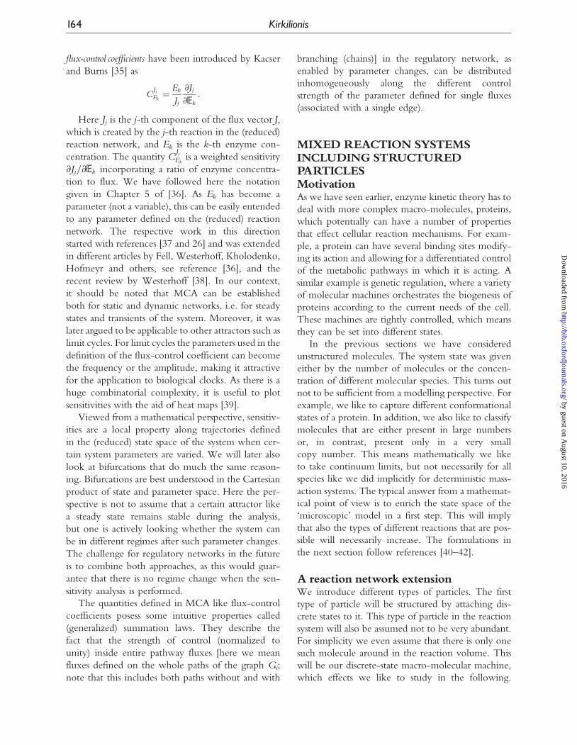
flux-control coefficients have been introduced by Kacser

and Burns [35] as

CJjEk ¼

Ek

Jj

@Jj@Ek

:

Here Jj is the j-th component of the flux vector J,which is created by the j-th reaction in the (reduced)

reaction network, and Ek is the k-th enzyme con-

centration. The quantity CJjEk

is a weighted sensitivity

@Jj=@Ek incorporating a ratio of enzyme concentra-

tion to flux. We have followed here the notation

given in Chapter 5 of [36]. As Ek has become a

parameter (not a variable), this can be easily entended

to any parameter defined on the (reduced) reaction

network. The respective work in this direction

started with references [37 and 26] and was extended

in different articles by Fell, Westerhoff, Kholodenko,

Hofmeyr and others, see reference [36], and the

recent review by Westerhoff [38]. In our context,

it should be noted that MCA can be established

both for static and dynamic networks, i.e. for steady

states and transients of the system. Moreover, it was

later argued to be applicable to other attractors such as

limit cycles. For limit cycles the parameters used in the

definition of the flux-control coefficient can become

the frequency or the amplitude, making it attractive

for the application to biological clocks. As there is a

huge combinatorial complexity, it is useful to plot

sensitivities with the aid of heat maps [39].

Viewed from a mathematical perspective, sensitiv-

ities are a local property along trajectories defined

in the (reduced) state space of the system when cer-

tain system parameters are varied. We will later also

look at bifurcations that do much the same reason-

ing. Bifurcations are best understood in the Cartesian

product of state and parameter space. Here the per-

spective is not to assume that a certain attractor like

a steady state remains stable during the analysis,

but one is actively looking whether the system can

be in different regimes after such parameter changes.

The challenge for regulatory networks in the future

is to combine both approaches, as this would guar-

antee that there is no regime change when the sen-

sitivity analysis is performed.

The quantities defined in MCA like flux-control

coefficients posess some intuitive properties called

(generalized) summation laws. They describe the

fact that the strength of control (normalized to

unity) inside entire pathway fluxes [here we mean

fluxes defined on the whole paths of the graph Gi;

note that this includes both paths without and with

branching (chains)] in the regulatory network, as

enabled by parameter changes, can be distributed

inhomogeneously along the different control

strength of the parameter defined for single fluxes

(associated with a single edge).

MIXEDREACTION SYSTEMSINCLUDING STRUCTUREDPARTICLESMotivationAs we have seen earlier, enzyme kinetic theory has to

deal with more complex macro-molecules, proteins,

which potentially can have a number of properties

that effect cellular reaction mechanisms. For exam-

ple, a protein can have several binding sites modify-

ing its action and allowing for a differentiated control

of the metabolic pathways in which it is acting. A

similar example is genetic regulation, where a variety

of molecular machines orchestrates the biogenesis of

proteins according to the current needs of the cell.

These machines are tightly controlled, which means

they can be set into different states.

In the previous sections we have considered

unstructured molecules. The system state was given

either by the number of molecules or the concen-

tration of different molecular species. This turns out

not to be sufficient from a modelling perspective. For

example, we like to capture different conformational

states of a protein. In addition, we also like to classify

molecules that are either present in large numbers

or, in contrast, present only in a very small

copy number. This means mathematically we like

to take continuum limits, but not necessarily for all

species like we did implicitly for deterministic mass-

action systems. The typical answer from a mathemat-

ical point of view is to enrich the state space of the

‘microscopic’ model in a first step. This will imply

that also the types of different reactions that are pos-

sible will necessarily increase. The formulations in

the next section follow references [40–42].

A reaction network extensionWe introduce different types of particles. The first

type of particle will be structured by attaching dis-

crete states to it. This type of particle in the reaction

system will also be assumed not to be very abundant.

For simplicity we even assume that there is only one

such molecule around in the reaction volume. This

will be our discrete-state macro-molecular machine,

which effects we like to study in the following.



Dow

nloaded from


The assumption of having one such particle can be

easily extended to any finite number. In contrast, the

second kind of particle is assumed to be small but

very abundant, like the ones we have modelled in

the mass-action reactions in ‘Mass action kinetics’

section. They will follow a birth–death process on

the microscopic level as before, i.e. they can also

appear and leave the system very frequently. This

kind of particle need not be structured, i.e. we

only take note of their numbers. Next we define

two sets of scales, a vector of size scales~� ¼ ð�1, . . . , �sÞ, di> 0 attached to each species of

small molecules (a typical interpretation is the aver-

age number of such particles in the system in some

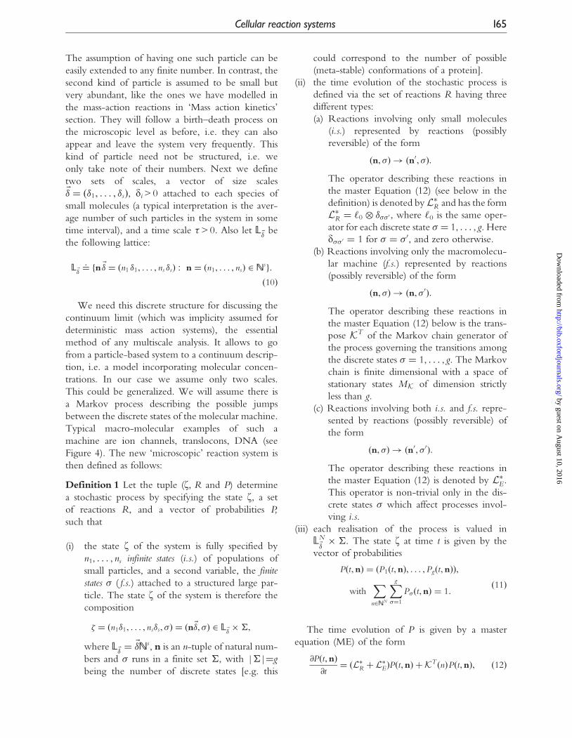
time interval), and a time scale � > 0. Also let L~�be

the following lattice:

L~�¼:fn ~� ¼ ðn1 �1, . . . , ns �sÞ : n ¼ ðn1, . . . , nsÞ 2 N

sg:

ð10Þ

We need this discrete structure for discussing the

continuum limit (which was implicity assumed for

deterministic mass action systems), the essential

method of any multiscale analysis. It allows to go

from a particle-based system to a continuum descrip-

tion, i.e. a model incorporating molecular concen-

trations. In our case we assume only two scales.

This could be generalized. We will assume there is

a Markov process describing the possible jumps

between the discrete states of the molecular machine.

Typical macro-molecular examples of such a

machine are ion channels, translocons, DNA (see

Figure 4). The new ‘microscopic’ reaction system is

then defined as follows:

Definition 1 Let the tuple (z, R and P) determine

a stochastic process by specifying the state z, a set

of reactions R, and a vector of probabilities P,such that

(i) the state z of the system is fully specified by

n1, . . . , ns infinite states (i.s.) of populations of

small particles, and a second variable, the finitestates � ( f.s.) attached to a structured large par-

ticle. The state z of the system is therefore the

composition

¼ ðn1�1, . . . , ns�s, �Þ ¼ ðn~�, �Þ 2 L~��,

where L~�¼ ~�Ns, n is an n-tuple of natural num-

bers and � runs in a finite set �, with |�|¼gbeing the number of discrete states [e.g. this

could correspond to the number of possible

(meta-stable) conformations of a protein].

(ii) the time evolution of the stochastic process is

defined via the set of reactions R having three

different types:

(a) Reactions involving only small molecules

(i.s.) represented by reactions (possibly

reversible) of the form

ðn, �Þ ! ðn0, �Þ:

The operator describing these reactions in

the master Equation (12) (see below in the

definition) is denoted byL�R and has the form

L�R ¼ ‘0 � ��0 , where ‘0 is the same oper-

ator for each discrete state � ¼ 1, . . . , g. Here

d��0 ¼ 1 for � ¼ �0, and zero otherwise.

(b) Reactions involving only the macromolecu-

lar machine (f.s.) represented by reactions

(possibly reversible) of the form

ðn, �Þ ! ðn, �0Þ:


the master Equation (12) below is the trans-

pose KT of the Markov chain generator of

the process governing the transitions among

the discrete states � ¼ 1, . . . , g. The Markov

chain is finite dimensional with a space of

stationary states MK of dimension strictly

less than g.(c) Reactions involving both i.s. and f.s. repre-

sented by reactions (possibly reversible) of

the form

ðn, �Þ ! ðn0, �0Þ:


the master Equation (12) is denoted by L�E .

This operator is non-trivial only in the dis-

crete states � which affect processes invol-

ving i.s.(iii) each realisation of the process is valued in

LN~��. The state z at time t is given by the

vector of probabilities

Pðt,nÞ ¼ ðP1ðt,nÞ, . . . ,Pgðt,nÞÞ,

withXn2NN

Xg�¼1

P�ðt,nÞ ¼ 1:ð11Þ

The time evolution of P is given by a master

equation (ME) of the form

@Pðt,nÞ@t¼ ðL

�R þ L

�EÞPðt,nÞ þ K

TðnÞPðt,nÞ, ð12Þ



Dow

nloaded from


with P, L�R, L�E and KT being sufficiently regular

such that (12) has a unique solution for all times

t> 0. Then the tuple (z,R, P) is called a (micro-

scopic) system with infinite and finite states, or short

an IFSS (Infinite-Finite State System).

Clearly, reactions of type (a) are the ‘traditional’

reactions, which in case there is no molecular

machine [and therefore no reactions of type (b)

and (c)] would lead us back to events described by

(1). But note in contrast to (1) we have not intro-

duced any chemical complex structure that would

need to be done in addition. Type (b) reactions

describe spontaneous changes of the states of the

molecular machine. They are not triggered by bind-

ing of small molecules to the machine. In contrast,

type (c) reactions combine the two previous types,

there is binding of the small molecule to the macro-

molecule which at the same time changes its state.

This reaction structure explains the structure of the

master Equation (12), which now in contrast to the

master Equation (2) becomes a vector equation with

as many components as there are discrete states of the

molecular machine. Note that we have not intro-

duced a complex structure for the master Equation

(12), this could be done in a similar way as for (2).

The same holds, therefore, for the limit equations

introduced in the next section.

The macroscopic equation and thecombined adiabatic and continuumlimits.The average dynamicsAs we could have done with master equation (2) to

derive deterministic mass-action kinetics, we can also

introduce deterministic limits for the vector Master

Equation (12). Because of the additional Markov

chain (MC) structure with which we describe the

molecular machines, there will be a combination of

two limits, a so-called adiabatic limit, and a contin-

uum limit. The adiabatic limit essentially assumes

that the MC consists of fast variables in comparison

with its environment, i.e. is in partial equilibrium

(this is the same as the QSSA in ‘QSSA’ section).

The equilibrium state of a MC is given by its

so-called invariant measure, which we will call .

The vector has as many components as the

master Equation (12). The continuum limit is a

large number limit on the microscopic time-

continuous Markov jump process describing the

small very abundant particles (molecules) of the

system. At the same time, the former discrete state

Figure 4: Shown are different examples of molecular machines that are best modelled as structured particles. (A) Atypical enzyme that can be in different states, either ‘silent’ or ‘active’ (usually associated with phosphorylation),and which only in its active state processes some substrate. (B) A string of DNA is shown, with binding sites to arepressor molecule which itself can be ‘inactivated’, i.e. by binding to some other smaller molecules looses the abilityto bind to the DNA string. Finally (C) Different membrane proteins, which act as protein translocation machines,or as ion channels, etc.



Dow

nloaded from


space becomes a continuous state space under this

operation, i.e. when letting the number n of mole-

cules of each such species tend to infinity. As it is

well known for the diffusion operator, this limit

can only be meaningful if at the same time the

vector of spatial scales ~� and the time scale � both

tend to 0 in a meaningful way. The continuum limit

is defined in terms of an expansion, where the

first-order term determines the deterministic vector

field, the second-order term describes the noise

terms, etc. [43]. As discussed, when introducing the

Gillespie algorithm (‘The Gillespie formulation of

stochastic mass-action kinetics’ section), the role of

noise is in itself a most interesting topic when dis-

cussing biological regulatory networks, but we will

omit it completely in the following. This means we

will only consider first-order terms in the expansion

defining the continuum limit. With these prepera-

tory remarks, i.e. when using a combination of adia-

batic and continuum limit in the way described, we

will get the following system of equation from (12):

dxiðtÞdt¼Xg�¼1

�ðxðtÞÞ fð�Þi ðxðtÞÞ,

xið0Þ ¼ xi, 0:

8<: ð13Þ

Here xi is the i-th concentration of a small

unstructured molecular species, 1 � i � s, � is the

�-th entry of and f ð�Þi is the �-th contribution of

the MC to the i-th component fi of the vector field fdescribing the dynamics of the different species

after up-scaling. For obvious reason Equation (13)

is also called average dynamics. Note that the average

vector field can be written in a matrix compact form:

_xðtÞ ¼ ðxðtÞÞFðxðtÞÞ, ð14Þ

with (x) ¼ (1(x), . . . ,g(x)) and FðxÞ ¼f f ð�Þi ðxÞg

�¼1,..., gi¼1,...s . We interpret Equation (14) as the

description of a regulatory network of s molecular

species, regulated by a single molecular machine

structured by g discrete states of an MC. This is

an alternative description when compared with

deterministic mass-action kinetics. Here we used

additional model ingredients and a new set of assump-

tions, i.e. the appearance of a regulatory machine

(single, so finite in number) that always works at

steady state, completely independent of the dynamics

of the regulatory network.

Application to synthetic biologyModel (14) can be used to represent detailed descrip-

tions of genetic reguatory networks. This is useful

when certain properties of genetic circuits are to be

designed synthetically [44]. Each genetic switch

involving a single gene is described as a molecular

machine in the sense described above. Transcription

factors are modelled as small unstructured particles.

The framework can be easily extended to a finite

number of molecular machines interacting via the

small unstructured molecules. This is very close

to the situation encountered in genetic regulation.

The framework can be used to systematically derive

governing equations for detailed regulatory mecha-

nisms, including DNA looping. An application

was given to model a synthetic clock in EscherichiaColi (Figure 5), and the thesis [45]. The resulting

equations are of the form (14).

STABILITY, ROBUSTNESSANDMODULARIZATIONOFREACTION SYSTEMSIn the following discussion on qualitative behaviour

of reaction networks, we restrict our attention again

to deterministic reaction systems, although the same

research could be carried out for stochastic systems

in most cases. Nevertheless, the mathematical tools

currently available are mainly based on the theory

of time-continuous dynamical systems, i.e. systems

of first-order differential equations. We will assume

that such an ODE system has been derived inside a

given modelling framework and with the help of

multiscale methods as discussed in previous sections.

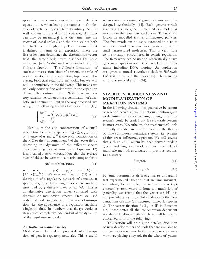
Let therefore

_x ¼ f ðxÞ, ð15Þ

xð0Þ ¼ x0 � 0, ð16Þ

be some autonomous (it is essential to understand

first experimental situations that are time invariant,

i.e. where, for example, the temperature is kept

constant) system where without too much loss of

generality we assume that the vector x 2 Rsþ has

components x1,x2, . . . ,xs that are descibing the con-

centrations of some (unstructured) molecular species

Si. The vector function f : Rsþ ! R

s in Equation

(15) incorporates all the concentration-dependent

non-linear feedbacks with which we will be mainly

concerned with in the following.

This section will be a quite detailed discussion

of new developments and tools that are available to

analyse reaction systems. In this respect, reaction net-

works are playing a key role for the whole of systems



Dow

nloaded from


analysis. We will first address the complexity of

solution behaviour for a given reaction system; for

example, the number of steady states in which the

system can be. Then we investigate whether the

steady states are stable, and perhaps are even global

attractors, making the system qualitatively very

simple. Nevertheless, with respect to the latter one

should realize that chemists in the 19th century

would have believed that any reaction system

goes asymptotically to a unique equilibrium state.

The conditions to posess a single globallly attracting

steady state are therefore an important case of refer-

ence. Any such questions on qualitative behaviour is

intimately related to the notion of robustness. We

like to know whether, for example, evolution has

favoured certain pathways or architectures, because

the cell or organism is less vulnerable to perturbations

of a certain kind. To answer such questions requires

in turn that we can define modules of the reaction

system in a meaningful way.

It will be important for our discussion that f will

be given at this stage (it will best have derived by one

or a combination of the methods described earlier in

this review. This would ensure its validity to describe

a specific experiment situation. In addition, the

model would have become better testable, for exam-

ple in the sense of Popper), and act on the network

of which the Si are the components (nodes). The

vector x0 determines the initial values of species

concentrations, i.e. set the conditions at the start of

experimental observation [Equation (16)]. Note that

mass-action systems (4) and (5), the derived enzyme

kinetics, the S-systems, the LV systems and the aver-

age dynamics (13) are such systems of non-linear

ODEs. It is, however, clear that perturbations of

f itself should also be considered, for example to

investigate structural stability questions.

The fundamental question in the following is

how to assign a network structure or graph G to

the couple (x, f ) such that the qualitative behaviourof (15) and (16) can be determined from the graph structure(network topology) (it should be noted that the same

question can be asked for the ‘microscopic’ stochastic

reaction systems following the master Equation (3).

This has been investigated for monomolecular

reactions in [9])?

Figure 5: Diagram of regulatory interactions in a synthetic clock consisting of two gene modules. The activatormodules consists of the structural gene glnG for the transcription factor NRI, driven by the NRI- responsiveglnAp2 promoter. The repressor module consists of the gene of the lac repressor, driven by the glnKp promoter.The circuit realizes an auto-activating feedback of the activator module, as the phosphorylated form of NRI, NRI-Pbinds to enhancer sites in the glnAp2 promoter, that enhance its activity. Second, negative feedback is realized byNRI-P stimulating the expression of the lac repressor via enhancer sites in the glnKp promoter. The lac repressorthen inhibits the expression of NRI by binding to lac operator sites inserted within the glnAp2 promoter of the acti-vation module. Additional low affnity (governor) sites for NRI in the glnAp2 promoter inhibitits activity when NRIconcentrations are high. Taken from Janus [45].



Dow

nloaded from


Other related ideas can be found in references

[46–48]. The question has a long tradition in eco-

logical research (see ‘Other qualitative behaviour of

[bio-chemical] regulatory networks’ section), and

was first asked by Robert May [49 and 50]. To get

started with this idea, we go back to the beginning

of this review. There we introduced the graph

G in order to systematically approach and investigate

a given cellular volume with respect to given molec-

ular binding events. The nodes of the graph G are

naturally associated with the species Si. After intro-

ducing averaging and up-scaling applied to the

elementary set of reactions given in (1), the ‘reaction

strength’ f could be derived on a ‘macroscopic’ scale

(in the sense of average of large particle numbers

inside any sufficiently small part of the reaction

volume). The complex structure of the reactions

(1) will determine which arrows are pointing to

some node now identified with xi, which is the

same in this view as listing the species concentrations

xi1, . . . , xil on which the i-th component of f is

depending on.

The interaction graphGIIt is possible to associate a weighted directed graph

GI to systems (15) and (16). The node set V incor-

porates the species concentrations (this is why in the

reaction kinetics literature, the interaction graph GI

is also called the species graph GS. Both graphs are

identical and just refer to different circimstances,

interaction is the more general concept acting between

components) xi, and the arrows in E are derived

from f. We do not incorporate the whole informa-

tion, but look at the linearization of f at any fixed

time t0 �0. This implies the arrows can change in

time, as we interpret the existence of a link to be

associated with a non-zero entry in the Jacobian J of

f evaluated at t0. The weights on the arrows are

given by the sign pattern of J( f ). As the signs can

change the weights on the arrows may also change.

Note that the network and weights are fixed for

equilibria of systems (15) and (16). The same is

true for a special class of non-linearities defining

the quasi-monotone differential equations [52], or (less

general, but with mathematically stronger results)

monotone systems [53]. We give an example of such

an interaction graph GI in Figure 6 describing a

Mitogen-activated protein kinase (MAPK) system,

as shown in Domijan and Kirkilionis [54].

As introduced, the question is how the graph

topology (evolving or fixed in time) determines the

qualitative behaviour. First we have to fix which

aspect of qualitative behaviour we like to or can

address. It turns out that the number of equilibria a

network might posess is an object that can be inves-

tigated with existing mathematical tools, and on basis

of the interaction graph GI. As the most prominent

example we state,

Theorem 1 (Thomas-Soule¤ ) If a system has no

positive cycles in GI(x) for any state x 2 Rnþ, then

it cannot exhibit multi-stationarity.

This original conjecture by Thomas was proven

by Soule in [51]. The positive cycles will be intro-

duced below in the context of feedback loops, but

they are easily intuitively explained when looking

at the example of a GI in Figure 6. We just need

to follow arrows with only positve signs and have to

be able to return to the same node.

Non-uniqueness of associated graphsIt has to be noted that once we have assembled an

interaction graph as a modelling device (as explained

in the first two sections of this review) and arrive at

systems (15) and (16), there are more different types

of graphs that we can associate with the ODE (and

perhaps other model frameworks, but that has not

yet been investigated). Typically the non-linearities

are further specified. Most results exist for mass-

action kinetics, where f becomes a polynomial

[see systems (4) and (5)]. Feinberg and co-workers

[55–59] have developed a theory for this case, where

during the process different types of graphs incorpor-

ating the complex set C ¼ fC1, . . . ,Ccg of a mass-

action system has been employed in different ways.

Incorporating the complex structure is mathemati-

cally intuitive, as this gives additional information

about the reaction system. The most often cited the-

orem in this context is (a variant of) the deficiency the-orem. The deficiency of a reaction network

(denoted by the symbol d) is defined by the formula

� ¼ c� l� �,

where c is again the number of complexes, l is the

number of linkage classes and � is the rank of

the stoichiometric matrix N . It holds that the defi-

ciency index is always non-negative [55]. We need

to define that complexes C and C 0 belong to the

same linkage class if there exists an undirected path

in the reaction diagram connecting the two com-

plexes. This defines l. The stochiometric subspace

for a reaction network is the span of the reaction



Dow

nloaded from


vectors, namely ImðN Þ. Two complexes (repre-

sented as vectors) C and C 0 are stoichiometrically

compatible if C0 � C 2 ImðN Þ. Stoichiometric

compatibility is an equivalence relation that induces

a partition of the space Rnþ into equivalence classes.

Each positive stoichiometric compatibility class is a

space of the form fx0 þ ImðN Þg \RNþ , where x0

is some positive initial concentration. We state the

following version of the deficiency theorems, as

given in Feinberg [57]:

Theorem 2 (Deficiency-ZeroTheorem) Consider

a mass-action reaction network of deficiency zero.

Assume that the network is weakly reversible [this

assumption is a weaker form of the requirement

that each of the reaction of the form (1) has a cor-

responding reaction in the reverse direction]. Then

the following holds for any arbitrary parameter set:

(1) The system admits neither a positive equilibrium,

nor a positive periodic orbit.

(2) The system has the following properties: each

positive stoichiometric compatibility class con-

tains precisely one equilibrium, this equilibrium

is asymptotically stable, and there is no

non-trivial periodic orbit.

The power of the deficiency-zero theorem is that

by definition of the deficiency index, we can identify

a class of networks that cannot have multiple positive

steady states. These networks can be very compli-

cated and contain hundreds of species. We also know

about the asymptotic stability of the resulting equi-

libria. Most of the different graphs associated with

deterministic reaction systems that can be found in

the literature have been reviewed in the Domijan

and Kirkilionis [54].

In conclusion, there are different types of graphs

that can be associated with a reaction system, there is

no uniqueness. The different graph topologies give

rise to different types of theorems making conclu-

sions about the possible dynamic behaviour of the

system. The complex structure of reaction networks

is usually exploited with much advantage. Existence

or non-existence of multiple steady states (equilibria)

for mass-action systems can be deduced from the

graph topology alone. This is very valuable as we

can decide, for example, whether a given system is

able to have switching behaviour (bistability, etc.).

Furthermore, we can rule out periodic solutions in

some cases. To make such conclusions, we need first

to fix the non-linearity f or the class of non-linearities

we like to investigate, so going the reverse way when

compared with the modelling process.

Other qualitative behaviour of[(bio-)chemical] regulatory networksAs we have already mentioned for LV systems (see

‘Lotka–Volterra systems’ section) other types of qual-

itative behaviour are of relevance. A typical question

in ecological food webs is whether the elimination of

a species will cause other species to be eliminated

from the system. Mathematically, this has been

investigated with the help of definitions like perma-

nence or persistence. Such questions are relevant for

genetic regulatory networks, where extinction can

be equivalent to knock-out of a certain gene. It is

surprising how little we know on how the choice of

certain non-linearities affect extinction behaviour. It

is generally agreed in ecology that this behaviour is

very sensitively reacting when non-linearities are

changed [60, 61], so either heuristic arguments or

mathematical derivation of the non-linearities used

really matters. Early work on chemical network sta-

bility are Clarke [62], Tyson [63] and Sontag [64].

Other types of qualitative behaviour can be used to

classify a certain type of non-linearity. For example,

we can ask how dense the set of mass-action kinetic

networks showing chaotic behaviour lies in the set of

general mass-action networks. Or about the stability

of topologically equivalent mass-action systems [65],

or their ability to produce arbitrary behaviour [66].

Such questions or classifications [67] are intimately

related to questions of feedback (see ‘Feedback loops’

section) and bifurcation behaviour (see ‘Bifurcation

analysis based on external currents’ section) [68, 69],

like the occurence of oscillating behaviour [70–76]).

The occurence of bistability is also relevant, as this is

necessary to construct biological switches [77, 78].

Feedback loopsFeedback loops are the essential objects to study any

non-linear system. They are, therefore, important to

understand any real-world problem that can be

investigated by measuring time series. In the context

of cell biology, it is the feedback loops of the various

regulatory networks that allow the cell to react to

new conditions, fine tune its own state, etc. The

most natural way to define feedback loops in a

given dynamical system (any dynamical system that

can be linearized in a well-defined way) is via the

interaction graph GI. The feedback loops there can

be defined by cycles of different length. A cycle in the



Dow

nloaded from


graph GI(x) is a sequence of distinct vertices

xi1, . . . , xik such that there is an edge connecting xi1to xi2, xi2 to xi3 and so on, finishing with an edge

between xik and xi1. The length of the cycle is the

number of vertices that it contains. The special case

of a cycle containing only one vertex is called a (self-

)loop. A loop has obviously length one and is asso-

ciated with the main diagonal entries of the Jacobian

matrix. Each cycle is endowed with a sign, which is

the product of the signs of its edges. In Figure 6, S1,

FS1 and F form a negative (sign) cycle in the inter-

action graph of the MAPK cascade. Some definitions

to feedback loops in mass-action systems can be

found in Sensse and Eiswirth [79].

MotifsThe motif concept is frequently encountered and

cited in the systems biology literature [80, 81]. It is

best discussed in the context of feedback loops. But

we will need to give several interpretations of a motif

in order to compare it with other concepts that are

previously introduced. In its simplest interpretation, a

motif is a certain type of sub-graph occuring multiple

times in a given network. For any given graph G, we

can indeed use methods from algebraic graph theory

(see for example, the classical text [82]) to count the

number of simple types of sub-graphs, for example

triangles (the complete graph K3), etc. Such an inves-

tigation leads to a spectral analysis of the graph G and

is an alternative characterization of the graph topol-

ogy. This is very helpful for very large graphs as it

allows to estimate whether the network topology is

more scale-free or exponentially distributed, etc. In

cell biology applications, it has been used for static or

evolving graph analysis; for example, to characterize

protein–protein networks (see ‘Static and evolving

network topologies, protien–protien networks’ sec-

tion). But can the concept of small sub-graph distri-

bution be of any use for understanding dynamic

regulatory networks, i.e. reaction networks? For

both conceptual and mathematical reasons this is

very unlikely. In this case, the network needs neces-

sarily be equipped with some dynamical process, as

explained in Figure 2. If we assume that the dyna-

mical network is defined, say by systems (15) and

(16) with a given non-linearity f, we must observe

that there is no theorem that would connect the

number of (a certain type of) sub-graphs with the

qualitative behaviour of the system. This is also not

to be expected, as it is the combination and linkage

of the feedback loops (as defined for the respective

interaction graph GI) inside the network that deter-

mines the dynamics, not the motif counting which

in fact seperates each such feedback loop represented

by the motif from its context, i.e. the other feed-

backs. It is therefore not feasible to take motifs as a

kind of architectural principle for dynamic regulatory

networks.

Of course, this does not exclude the necessity and

importance to study simple (genetic) regulatory

interactions in experimental isolation from other

feedback loops. It is not surprising that this is exactly

what can be found in the literature [83].

Modules and stoichiometric networkanalysis: extremal currents (elementaryflux modes)The so-called stoichiometric network analysis (SNA)

was introduced in a seminal paper by Clarke [84],

and is one of the most prominent methods of

analysing chemical and biochemical networks of

mass-action type, i.e. systems (4) and (5). Note that

if rankðN Þ ¼ � � s (s was the number of species),

then the reaction system has (s - �) conservation

relations [36]. A conservation relation is a relation

between a set of species with their total concentra-

tion being preserved. The set of conservation rela-

tions takes the form

gTl x ¼ cl, l ¼ 1, . . . , s� �,

Figure 6: The interaction graph GI (same as speciesgraph GS). The nodes show the different species names.Example taken from Domijan and Kirkilionis [54].



Dow

nloaded from


where each gTl 2 kerðN Þ and cl 2 Rþ is a constant

describing the total conserved concentration. The set

of conservation relations forms an invariant space

[85]. Non-trivial equilibria of the network (we char-

acterize their constant state here by x0) for a chosen

set of parameters (reaction constants) k0 are deter-

mined by the conditions

N vðx0, k0Þ ¼ 0, ð17Þ

x0 > 0: ð18Þ

Any such equilibrium clearly depends on the

kinetic parameters k 2 Rrþ (r was the number of

reactions), but also on the constants cl, l ¼ 1, . . . ,

s-� stemming from the conservation relations. Due

to (17) and (18), all stationary reaction rates belong to

an intersection of the kernel of N and the positive

orthant of the reaction space,

vðx0, k0Þ 2 z 2 R�jN z ¼ 0, z 2 R

�þ

� �¼ KerðN Þ \R

sþ,

ð19Þ

which form a convex polyhedral cone Kv [86].

This cone Kv is spanned by a set of minimal gener-

ating vectors Ei’s (called extremal currents, as intro-

duced in Clarke [84]):

Kv ¼Xt

i¼1

jiEi : ji > 0 8 i

( ):

These generating vectors are unique up to scaling

by a positive constant. They may be linearly depen-

dent, as the number of extreme currents (better

known as elementary flux modes in the systems biol-

ogy literature) may be greater than dimðkerðN ÞÞ.Extreme currents decompose the network into min-

imal steady state-generating sub-networks. We can

also call these sub-networks modules, an important

concept in cell biology [87, 88]. A current corre-

sponds to a certain subset of the reaction set which

when assembled into a dynamical system by the

assumption of mass-action kinetics can produce pos-

itive equilibria (independent on the rest of other

reactions not part of this specific extremal current).

In the biochemical literature, they are interpreted as

switching on or off different parts of a metabolic

pathway associated with the current. Mathematically,

due to the polynomial RHS of mass-action net-

works, extremal currents are the best known exam-

ple to know how to split a non-linear dynamical

network into what could be called ‘modules’ or

functional units. They clearly qualify as an architec-

tural building block principle for complex networks.

But note that the splitting relies on the equilibrium

assumption.

The influence of a sub-network on the full net-

work dynamics (i.e. how much the given subnet-

work plays a part in creating a certain steady state)

depends on the constants ji’s, which are called

convex parameters. In fact the Jacobian of the net-

work evaluated at any positive steady state, x0, can

be written as a convex combination of contributions

from the extreme currents:

DxN vðx0,k0Þ2XMi¼1

jiN diagðEiÞ�TdiagðhÞ : ji>0,h2R

mþ

( ):

ð20Þ

Here h is a vector defined as the inverses of any

equilibrium concentrations x0, � the matrix of stoi-

chiometric exponents (note, usually �ij ¼ �ij, i.e. the

stiochiometry of the reactants in each reaction) (see

‘Mass-action Kinetics’ section) and diag(v) is a diag-

onal matrix with the diagonal entries given by the

vector v. The contribution of a single extreme cur-

rent is given by the term

jiN diagðEiÞ�TdiagðhÞ,

which represents the Jacobian of the subnetwork

generated by the extreme current Ei, evaluated at

any of its positive steady states. The Jacobian descrip-

tion in the form of (20) comes from a simple obser-

vation that for positive steady states x0,

DxN vðx0, k0Þ ¼ Ndiagðvðx0, k0ÞÞ�Tdiagðx�1

0 Þ: ð21Þ

Together with the newly defined parameters,

hs ¼ x�1s , s¼ 1, . . . , n, the convex parameters

j replace the reaction constants k and the conserved

mass constants c.

Stability analysis and characterization of regulatorynetworks by extremal currentsWe can use the elementary current concept to

investigate whether a combination of sub-networks

giving rise to asymptotically stable (here we need a

slightly stronger stability concept, i.e. mixing stability)positive equilibria produces such equilibria on the

system level, i.e. whether the linear combination of

stable sub-networks as given in (20) produces stable

positive equilibria for the whole network [19]. It is

important to characterize the dynamical stability

of equilibria of extremal currents. It has been pro-

posed in Stelling et al. [89] that extremal currents

(without stability analysis) could serve as a structural

characterization of cellular regulatory networks.



Dow

nloaded from


The advantage of the extremal currents is indeed that

they can be computed without the knowledge of

kinetic parameters, as they only depend on the

stoichiometric matrix and the positivity condition

(17,18). Unfortunately, the problem arises that

most of the currents might be unstable, so their

simple counting can be misleading as they do not

correspond to feasible physiological states. Regula-

tion and feedback are dynamic properties and cannot

be captured by a measure neglecting both weights

on vertices and edges of the associated interaction

graph GI (Figure 2). On the other hand, the extremal

currents are able to address stability questions of

equilibria [Equation (21)], so there is no need to

neglect this additional information.

Bifurcation analysis based on extremal currentsIn a series of papers, Karin Gatermann has introduced

methods from algebraic geometry, which in combi-

nation with the extremal current formalism allow to

analyse bifurcations [18, 19, 90–92] away from equi-

libria. The results have been recently summarized

and extended in Domijan and Kirkilionis [93]. In

classical bifurcation theory, the behaviour of the

reaction system would depend on the parameters kiand ci. It was noted by Karin Gatermann that

when bifurcation theory is applied to SNA, this

requires some additional restrictions on the con-

vex polyhedral cone (19). In SNA, every ray in the

convex cone, i.e. [z1, . . . ,z�] with z 2 kerðNÞ \R�þ,

corresponds to some positive solution of (17) for

some values of k. To find such a positive solution

x it is sufficient to solve the system

z ¼ vðx, kÞ ¼ x0vðx, kÞ, ð22Þ

where the constant x0 is introduced because of the

ambiguous length of z. The construction is such

that the interior of the convex cone corresponds to

all positive solutions of (17) for any value of k.However, for fixed values of k and a given z> 0, a

solution for the system (22) is not guaranteed. In fact,

z needs to satisfy additional conditions that have

been derived in Gatermann [18]. Using this, a pos-

itive solution exists if, and only if, z 2 VðIdeftor Þ where

VðIdeftor Þ is an affine deformed toric variety of the

deformed toric ideal,

Ideftor ¼ f 2 Q½zj f ðvðx; kÞÞ ¼ 0� �

QðkÞ½z:

Since each ray of the cone is parametrized by a

different choice of convex parameters j, there are also

restrictions on j. Positive solutions will exist if

j 2 VðJÞ \RMþ , where V(J) is a variety of the new

ideal created by substituting z ¼PM

i¼1 jiEi into Ideftor .

In conclusion, we have gained an algebraic method

which when varying a ji later as a bifurcation param-

eter at the same time the existence of corresponding

positive equilibrium solutions of the reaction system

can be guaranteed under above conditions. In

Domijan and Kirkilionis [93], this has been used

to characterize (among others) saddle-node and

Hopf-bifurcations, which by using the j parameters

can be discussed in relationship to the contributions

of different reaction sub-networks, i.e. the ones

given by extremal currents.

PRESENT SITUATIONANDOUTLOOKThe current situation in the field of cellular reaction

networks is very heterogeneous, and there is prob-

ably a lot of confusion even among experts. The

author agrees strongly with Hans Westerhoff

in [38] who refering to the most interesting publica-

tion of Heinrich [94] also addresses this ‘Babylonian

confusion’ in the area, making at the end of his paper

a very illustrative example of how difficult it is for

the human mind to understand what regulates what

in a biochemical context. Heinrich (the author dis-

cussed with Heinrich shortly before his sudden death

in a cafe in Yokohama, Japan, during an interna-

tional systems biology conference) pointed out in

his publication [94] that the major problem is the

use of different scientific languages and something

that could be called different ‘points of view’. The

problem is indeed a general one and therefore effects

heavily a newly emerging field like systems biology,

where many different scientific disciplines are con-

tributing. Perhaps everybody from mathematician,

computer scientist, physicist, up to chemist and biol-

ogist uses a different language and looks very differ-

ently at the (same) situation. This makes the area very

interesting for a philosopher of science, and more

work on this should be encouraged. The situation

is even more delicate because network theories are at

the core of another newly emerging sience, complex

systems theory. In the end of course it is scientific

success that counts, and this means predictive abili-

ties. Not every concept can achieve this in every

circumstance, there are indeed theories that need

to be refused due to their lack of predictive power

during the scientific progress. Of course, there is



Dow

nloaded from


plurality in the questions being asked, this is a par-

ticular strong point of systems biology at the

moment.

Derivation of reaction network modelsAs a mathematician the author would like to support

the idea that different approaches follow a hierachical

organization, and that, therefore, there should exist

mathematical ways to derive observational quantities

of a reaction network model from microscopic inter-

actions. Here ‘microscopic’ is used in the sense that

the basic events (or rules) of such an interaction can

be well characterized and are self-consistent, i.e.

there is no further deeper level that would signifi-

cantly contribute to the behaviour of the chosen

microscopic level. This thinking is indeed how this

review is organized, starting with the basic event of

reaction systems, the reaction event, (1). It is not so

much that every theory would need to start on this

level. But it has an enormous advantage to know that

a theory can be traced back to basic events or rules in

a given situation, at least in principle. A recipe for

up-scaling and derivation of the dependent variables

(observables) of the model is one way to achieve this

goal. Such principles also guarantee that the quanti-

ties involved can be interpreted, and what it means

measuring them. As an example, Westerhoff in [38]

is right in his argument that a theory like MCA (see

‘Metabolic control analysis’ section) did contribute to

clarify and therefore make control of enzymatic

pathways ‘measureable’, simply because it became

well-defined what quantities have what meaning in

the context of regulation. It should be noted, how-

ever, that MCA itself is already a high level, i.e.

macroscopic and derived theory as explained in this

review (it is clear that, for example, membrane pro-

teins have a different event statistics than freely dif-

fusing enzymes, and this would lead to different

MCA variants). The context of scales is most impor-

tant when discussing regulation in cell biology. Scales

are a natural object in physics and mathematics, but

as discussed often neglected in the computer science

area.

Regulation and graph theoryThe review stressed the use of graphs to understand

regulatory pathways. The graphs have been used for

two different purposes. First as a tool to assemble a

model of a regulatory network from scratch. Second

to deduce the qualitative behaviour of the network

from a graph attached to an existing reaction

mechanism. The two aspects have to be strictly sepa-

rated. The use of graphs to sketch relationships

between certain components is very valueable, espe-

cially in biology. Different such diagrams and con-

ventions exist; for example, in genetics. But it should

be emphasized that the meaning of the relationships

becomes only clear when, for example, the right

time-scales of different processes have been set up.

Which in other words means the weights drawn in

Figure 2 have been properly set up. This coincides

with the step-wise procedure that a dynamical

system has been derived which then constitutes (in

a further step) a measurable model or hypothesis that

becomes refutable, i.e. scientific.

Inference of network architecture andparameter estimationWe have not discussed any methods of statistical

inference or parameter fitting in this review. This

has been done on purpose. A comprehensive

review article for reaction mechanisms is Crampin

et al. [96]. The review discussed what we could

name ‘forward modelling’, i.e. a model is constructed

from first principles as good as possible. In a next

step, the model produces a time series (in ‘forward’

direction, i.e. with time following the time arrow),

which can then be compared with data. The idea

was to restrict ourselves to cases where spatial posi-

tion of molecules can be neglected. This might not

always be possible. Not only because of the impor-

tance of spatial gradients in cells, but also because

reaction and transport are often intertwined, for

example, in so-called ‘crowded environments’, and

because different types of molecules will have differ-

ent restrictions in their movements in the cell [97–

99]. We are just at the beginning to understand the

implications of such observations for the behaviour

of reaction networks. With respect to system identi-

fication, we must find better ways to bring together

methods from reaction networks with statistical

approaches, like Bayesian networks. The latter are

often used to interpret micro-array and other genetic

data, most often not given as a time series. It is nev-

ertheless clear that even micro-array data must stem

finally from regulatory interactions (typically mea-

sured from a number of cells in a tissue), which

should be able to be described by models as pre-

sented in this review. A confirmed reaction mecha-

nism should constitute additional information that

can be incorporated into a Bayesian approach.



Dow

nloaded from


Relevance for bioinformaticsFor bioinformatics this means that it enters new ter-

ritory when dealing with cellular reaction systems

and regulation. In reaction networks there is always

a mixture of discrete and continuous objects, i.e.

there are not exclusively discrete objects. As out-

lined, rule-based systems must become rate-based

systems when a comparison with time-series is envi-

saged. It should be remembered that bioinformatics

had its great breakthroughs in sequence analysis, a

completely discrete method. Non-discreteness

makes it harder to implement algorithms, as notions

like approximation and averaging stemming from

applied non-linear analysis will be definitely

needed. On the other hand, discrete concepts from

computer science, like methods from membrane

computing [95], can offer new opportunities when

combined with analysis techniques. It is the opinion

of the author that purely discrete and static (i.e.

non-temporal) network concepts, like the motifs

(see ‘Motifs’ section), are not the correct way to cap-

ture the properties of regulatory pathways.

We should also remind ourselves that bioinfor-

matics has its strength in automatisation of informa-

tion retrieval. For example, data-mining techniques

are playing an important part in that respect. It has

been tried to incorporate information on dynamical

behaviour into databases; for example, Kyoto

Encyclopedia of Genes and Genomes. In many

respects, it is still too early for making automatic

reaction network models. The kinetic data are too

unreliable and really depend on the specific environ-

ment in which they are measured. There is currently

no way around the fact that scientists who think

about a specific regulatory pathway need to propose

a model and design specific experiments to verify

their hypothesis. This does not mean that a more

automatized creation of reaction network models

should not be supported. Clearly this would help

and speed up the modelling process itself. But at

the moment, it is likely that there needs to be a

critical mind in the background that is asking about

the implicit assumptions being made while the reg-

ulatory model is assembled.

Open problemsThere are many open and challenging problems in

the field. We have already touched many situations

where essential gaps in the theory did occur. The

following list is made to encourage research in the

area, but is of course not complete. We follow

the sections of the review. Stated are mainly math-

ematical problems, which also should at the same

time improve the applicability of the tools described

in the review inside bioinformatics.

P1 (Mathematical Problem) There are many math-

ematical questions related to the ‘rate conversion’

of rule-based systems (see ‘Rule-based networks’

section). Can we, for example, define simple

conditions such that the rate converted

rule-based system asymptotically for t!1converges to the same attractor as before, i.e. as

the deterministic non-rate converted rule-based

system did? Think about this problem in terms of

Boolean networks or networks with a small

number of discrete states. Can we allow some

randomness of evaluation of the rules that are

of Gillespie type, i.e. take combinatorial effects

into account?

P2 (Mathematical Problem) A related problem to P

1 is about the discretization of continuous state

spaces or of general non-linearities f, the weights

on the edges of the interaction graph GI. There

is already a rich literature on so-called piecewise

linear f replacing the original non-linearity. It is a

natural question to ask for consistency and error

estimates, i.e. if the number n of intervals on

which f is linear converges to infinity, the

system has the same qualitative behaviour as

the original one. Does this property hold already

for finite but large n? Are there theorems spec-

ifying n and the length and positions of the

respective intervals such that the consistency

condition holds? With respect to discretization

of continuous state spaces, there are similar ques-

tions that have already been stated. Define an

equivalence between the type and number of

attractors of the discrete and continuous state

network. This definition should also describe

the exact relationship between the rate-based

rule or event structure of both the discrete and

the continuous network, i.e the ‘fluxes’. For

which such definitions or assumptions do dis-

crete and continuous dynamics on networks

coincide? If this is not possible to decide, are

there rational choices of discrete state spaces

and their size given a time series stemming

from a cellular regulatory network?

P3 (Mathematical Problem) This problem is about

extensions of the Thomas-Soule result in ‘The

interaction graph’ section on the interaction



Dow

nloaded from


graph GI. There are obviously many possible

ways of extensions. It should be noted that the

Thomas-Soule theorem makes no statement

about the stability or instability of steady states.

This is in contrast to the deficiency theorem pre-

sented in ‘Non-Uniqueness of associated graphs’

section, where the RHS f is a polynomial (due to

the fact that mass-action kinetics has been used).

Can stability results be incorporated to theorems

of Thomas-Soule type if we specify a class of

non-linearities? Does for example the following

hold: Assume f is (quasi-)monotone, and GI has

no positive cycles (in this case we do not need to

specify for which states x GI has this property). If

a unique positive steady state exists, then it is

globally asymptotically stable.

P4 (Mathematical Problem) Can elementary currents

[see ‘Modules and stoichiometric network analy-

sis: external curents (elementary flux models)’

section] as a constructive idea and design principle

be generalized to non-polynomial reaction net-

works, i.e. is there a natural ‘modularisation’ in

terms of sub-networks that are able to exhibit

positive steady states? Can then the overall

system behaviour be analysed as linear combina-

tions of these sub-networks?

P5 (Computer Science and Mathematics) Can

elementary currents [see ‘Modules and stoichio-

metric network analysis: external curents (ele-

mentary flux models)’ section) be implemented

efficiently as a research tool where biological

switches and oscillatory behaviour can be con-

structed by reverse engineering? Can this be com-

bined with MCA (see ‘Metabolic control analysis’

section), i.e. can we generalize beyond stability

results and incorporate sensitivity analysis?

Key Points

� Reaction networks are a key tool for understanding cellular pro-cesses. At the same time they are thebest investigated examplesof dynamic complex networks and therefore play again a keyrole for other areas of applications.

� Due to their dual basis in both discrete mathematics (graphtheory) and time-continuous dynamical systems, they still offermany conceptual challenges.

� There are also experimental challenges due to the need of mea-suring detailed time-series inside the cell. To approach thesechallenges is a key scientific question in the coming years andwill help to develop new drugs and therapies.

� The review discusses in detail different graphs that can be asso-ciated with reaction systems in order to retrieve knowledge onthe qualitative behaviour of the system.

References1. Collins SR, Schuldiner M, Krogan NJ, Weissman JS.

A strategy for extracting and analyzing large-scale quantita-tive epistatic interaction data. Genome Biol 2006;7:R63.

2. Schuldiner M, Collins SR, Weissman JS, Krogan NJ.Quantitative genetic analysis in Saccharomycescerevisiae using epistatic miniarray profiles (E-MAPs) andits application to chromatin functions. Methods 2006;40:344–52.

3. King RD, et al. The automation of science. Science 2009;324(5923):85–9.

4. Jeong H, Mason SP, Barabasi A-L, Oltvai ZN. Lethality andcentrality in protein networks. Nature 2001;411:41–2.

5. Gnad F, Oroshi M, Birney E, Mann M. MAPU 2.0:high-accuracy proteomes mapped to genomes. NucleicAcids Res 2009;37(Database issue):D902.

6. Sole R, Pastor-Satorras R, Smith E, Kepler TB. A model oflarge-scale proteome evolution. ACS 2002;5:43–4.

7. Jeong H, Tombor B, Albert R, et al. The large-scaleorganization of metabolic networks. Nature 2000;407:651–4.

8. Ricard J. Reduction, integration and emergence inbiochemical networks. Biol Cell 2005;96(9):719–25.

9. Gadgil C, Lee CH, Othmer HG. A stochastic analysis of first-order reaction networks. BullMathBiol 2005;67:901–46.

10. Horn F, Jackson R. General mass action kinetics. ArchRationMech Anal 1972;48:81.

11. Gillespie DT. A general method for numerically simulatingthe stochastic time evolution of coupled chemical reactions.J Comput Phys 1976;22:403–34.

12. Rathinam M, Petzold LR, Cao Y, Gillespie DT. Stiffnessin stochastic chemically reacting systems: the implicittau-leaping method. J Chem Phys 2003;119:12784.

13. Gillespie DT, Petzold LR. Improved leap-size selectionfor accelerated stochastic simulation. J Chem Phys 2003;119:8229.

14. Evans TW, Gillespie CS, Wilkinson DJ. The SBML discretestochastic models test suite. Bioinformatics 2008;24(2):285.

15. Li H, Cao Y, Petzold LR, Gillespie DT. Algorithms andsoftware for stochastic simulation of biochemical reactingsystems. Biotechnol Prog 2008;24(1):56–61.

16. Kauffman SA. The Origins of Order. Self Organization andSelectioninEvolution. Oxford: Oxford University Press, 1993.

17. Walter W. Ordinary Differential Equations. New York:Springer, 1998.

18. Gatermann K. Counting stable solutions of sparse poly-nomial systems in chemistry. Symbolic computation:solving equations in algebra, geometry, and engineering.In: Green E., Hosten S., Laubenbacher R., Powers V.,(eds). Contemporary Mathematics. Vol. 286. Providence:American Mathematical Society, 2001;53–69.

19. Sensse A. Convex and toric geometry to analyze complexdynamics in chemical reaction systems. PhD Thesis. Otto-von-Guericke-Universitat: Magdeburg, 2005.

20. Hoops S, Sahle S, Gauges R, et al. COPASI – a COmplexPAthway SImulator. Bioinformatics 2006;22(24):3067.

21. Savageau MA. Biochemical systems analysis. I. Some math-ematical properties of the rate law for the component enzy-matic reactions. JTheor Biol 1969;25:365–9.



Dow

nloaded from


22. Savageau MA. Biochemical Systems Analysis: A Study ofFunction and Design in Molecular Biology. Boston: Addison-Wesley, 1976.

23. Savageau MA. A critique of the enzymologists test tube. In:Bittar EE (ed). Fundamentals of Medical Cell Biology, Vol. 3a.New York: Academic Press, 1992;45108.

24. Eigen M, Schuster P. The catalytic hypercyclea principleof precellular organization. Die Naturwissenschaften 1977;64:541–65.

25. Hofbauer J, Sigmund K. The Theory of Evolution andDynamical Systems. Cambridge University Press, 1988.

26. Heinrich R, Rapoport TA. A linear steady-state treatmentof enzymatic chains. General properties, control and effectorstrength. Eur J Biochem 1974;42:89–94.

27. Palsson BO, Palsson H, Lightfoot EN. Mathematicalmodelling of dynamics and control in metabolicnetworks. III. Linear reaction sequences. JTheor Biol 1985;113:279–98.

28. Keener J, Sneyd J. Mathematical Physiology. Heidelberg:Springer, 1998.

29. Fall CP, Marland ES, Wagner JM, Tyson JJ. ComputationalCell Biology. Interdisciplinary Applied Mathematics, Vol. 20.Heidelberg: Springer, 2004.

30. Murray J. Mathematical Biology, Vol. I and II, 3rd edn.Heidelberg: Springer, 2002.

31. Edelstein-Keshet L. Mathematical Models in Biology.Philadelphia: SIAM, 2005.

32. Siegel IH. Enzyme Kinetics. Hoboken: Wiley, 1975.

33. Deuflhard P, Heroth J. Dynamic dimension reduction inODE models. In: Keil F, et al (eds). Scientific Computing inChemical Engineering. Heidelberg: Springer, 1996, 29–43.

34. Rheinboldt WC. Dfferential algebraic systems as diferentialequations on manifolds. Math Comp 1989;3:73–482.

35. Kacser H, Burns JA. The control of flux. SympSoc Exp Biol1973;27:65–104.

36. Heinrich R, Schuster S. The Regulation of Cellular Processes.London: Chapman & Hall, 1996.

37. Heinrich R, Rapoport TA. Linear theory of enzymaticchains; its application for the analysis of the crossover the-orem and of the glycolysis of human erythrocyte. Acta BiolMed Ger 1973;31:479–94.

38. Westerhoff HV. Signalling control strength. J theor Biol2008;252:555–67.

39. Rand D. Mapping global sensitivity of cellular networkdynamics: sensitivity heat maps and a global summationlaw. J RSoc 2008;6(5):59–69.

40. Sbano L, Kirkilionis M. Molecular Reactions Describedas Infinite and Finite State Systems. Part I: ContinuumApproximation. Coventry, arXiv.org: arXiv:0802.4259v2,Warwick Preprint, 05/(2007).

41. Sbano L, Kirkilionis M. Molecular Reactions Described asInfinite and Finite State Systems. Part II: Deterministic Dynamicsand Examples. Coventry: arXiv.org: arXiv:0802.4279v1,Warwick Preprint, 07/(2007).

42. Sbano L, Kirkilionis M. Multiscale analysis of reaction net-works. Theory Biosci 2008;127:107–23.

43. Pavliotis GA, Stuart AM. An Introduction to MultiscaleMethods. Springer, 2008.

44. Hasty J, McMillen D, Collins JJ. Engineered gene circuits.Nature 2002;420:224–30.

45. Janus U. Modeling and Analysis of AGenetic Oscillator in E.coli.Coventry: University of Warwick, 2009.

46. Tyson JJ, Chen K, Novak B. Network dynamics and cellphysiology. Nat RevMol Cell Biol 2001;2:908–16.

47. Ebenhoh O, Heinrich R. Stoichiometric design ofmetabolic networks: multifunctionality, clusters, optimiza-tion, weak and strong robustness. Bull Math Biol 2003;65:323–57.

48. Hofmeyr J-HS, Westerhoff HV. Building the cellularpuzzle. Control in multi-level reaction networks. J TheorBiol 2001;208:261–85.

49. May R. Stability and complexity in model ecosystems.Monographs in Population Biology. Princeton: UniversityPress, 1973.

50. May R, Levin S, Sugihara G. Ecology for bankers. Nature2008;451(21):893–5.

51. Soule C. Graphic requirements for multistationarity.ComplexUs 2003;1:123–33.

52. Kirkilionis M, Walcher S. On comparison systems forordinary differential equations. J Math Anal Appl 2004;229(1):157–73.

53. Smith HL. Monotone Dynamical Systems: An Introduction to theTheory of Competitive and Cooperative Systems. Providence,Rhode Island: American Mathematical Society, 1995.

54. Domijan M, Kirkilionis M. Graph Theory and QualitativeAnalysis of Reaction Networks. Networks and HeterogeneousMedia 2008;3:95322.

55. Craciun G, Tang Y, Feinberg M. Understanding bistabilityin complex enzyme-driven reaction networks. PNAS 2006;30(103):8697–702.

56. Feinberg M. Complex balancing in general kinetic systems.Arch RationMech Anal 1972;49:187–94.

57. Feinberg M. The existence and uniqueness of steady statesfor a class of chemical reaction networks. Arch RationMechAnal 1995;132:311–70.

58. Feinberg M, Ellison P. The chemical reaction network toolbox.http://www.chbmeng.ohio-state.edu/feinberg/crnt.

59. Craciun G, Feinberg M. Multiple equilibria in complexchemical reaction networks: I. The injectivity property.SIAMJAppMath 2005;65:1526–46.

60. Moore PD. Roots of stability. Nature 2005;437(7061):959–61.

61. Holt RD. Asymmetry and stability. Nature 2006;442(7100):252–53.

62. Clarke BL. Theorems on chemical network stability. JChemPhys 1975;62:773–75.

63. Tyson JJ. Classification of instabilities in chemical reactionsystems. J Chem Phys 1975;62:1010–15.

64. Sontag E. Structure and stability of certain chemical net-works and applications to the kinetic proofreading model ofT-cell receptor signal transduction. IEEETransAutomatContr2001;46:1028–47.

65. Clarke BL. Stability of topologically similar chemical net-works. J Chem Phys 1975;62:3726–38.

66. Perelson AS, Wallwork D. The arbitrary dynamic behaviorof open chemical reaction systems. J Chem Phys 1977;66:4390–4.

67. Eiswirth M, Freund A, Ross JJ. Mechanistic classification ofchemical oscillators and the role of species. Adv Chem Phys1991;80:127–99.



Dow

nloaded from

http://www.chbmeng.ohio-state.edu/feinberg/crnt


68. Guckenheimer J, Holmes JP. Nonlinear oscillations, dyna-mical systems and bifurcations of vector fields. Appl MathSci, Vol. 42. Heildelberg: Springer, 1983.

69. Kuznetsov Y. Elements of applied bifurcation theory. ApplMath Sci, 112. Heildelberg: Springer, 1984.

70. Goldbeter A, Dupont G. Allosteric regulation, cooperativ-ity, and biochemical oscillations. Biophys Chem 1990;37:341–53.

71. Clarke BL, Jiang W. Method for deriving Hopf and saddle-node bifurcation hypersurfaces and application to a modelof the Belousov-Zhabotinskii reaction. J Chem Phys 1993;99:4464–76.

72. Field RJ, Koros E, Noyes RM. Oscillations in chemicalsystems. 2. Thorough analysis of temporal oscillation inbromate-cerium-malonic acid system. J Am Chem Soc1972;94(25):8649–64.

73. Field RJ, Noyes RM. Oscillations in chemical systems. IV.Limit cycle behavior in a model of a real chemical reaction.J Chem Phys 1974;60:1877–84.

74. Selkov EE. Self-oscillations in glycolysis. 1. A simple kineticmodel. EurJ Biochem 1968;4:79–86.

75. Krischer K, Eiswirth M, Ertl G. Oscillatory CO oxidationon Pt(110): modeling of temporal self-organisation. JChemPhys 1992;96:9161–72.

76. Bronnikova TV, Fed’kina VR, Schaffer WM, Olsen LF.Period-doubling bifurcations in a detailed model of theperoxidase-oxidase reaction. J Phys Chem 1995;99:9309–12.

77. Aguda BD, Clarke BL. Bistability in chemical reaction net-works: theory and application to the peroxidase-oxidasereaction. J Chem Phys 1987;87:3461–70.

78. Slepchenko BM, Terasaki M. Cyclin aggregation androbustness of bio-switching. Mol Biol Cell 2003;14:4695–706.

79. Sensse A, Eiswirth M. Feedback loops for chaos in activator-inhibitor systems. J Chem Phys 2005;122:044516.

80. Milo R, Shen-Orr S, Itzkovitz S, et al. Network motifs:simple building blocks of complex networks. Science 2002;298:824–7.

81. Alon U. Network motifs: theory and experimentalapproaches. Nat Rev Genet 2007;8:450–61.

82. Biggs N. Algebraic Graph Theory. Cambridge: CambridgeUniversity Press, 1974.

83. Kaplan S, Bren A, Dekel E, Alon U. The incoherent feed-forward loop can generate non-monotonic input functionsfor genes. Mol Sys Biol 2008;4:203.

84. Clarke BL. Stability of complex reaction networks. AdvChem Phys 1980;43:1–216.

85. Volpert A, Hudyaev S. Analysis in Classes of DiscontinuousFunctions and Equations of Mathematical Physics (Chapter 12).Dordrecht: Martinus Nijhoff, 1985.

86. Rockafeller RT. Convex Analysis. Princeton: PrincetonUniversity Press, 1970.

87. Hartwell LH, Hopfield JJ, Leibler S, Murray AW.From molecular to modular cell biology. Nature 1999;402:C47–52.

88. Sole RV, Valverde S. Spontaneous emergence ofmodularity in cellular networks. J R Soc Interface 2008;5(18):129–33.

89. Stelling J, Klamt S, Bettenbrock K, etal. Metabolic networkstructure determines key aspects of functionality and regula-tion. Nature 2002;420:190–3.

90. Gatermann K, Eiswirth M, Sensse A. Toric ideals and graphtheory to analyze Hopf bifurcations in mass-action systems.J SymbComp 2005;40:1361–82.

91. Gatermann K, Wolfrum M. Bernstein’s second theoremand Viro’s method for sparse polynomial systems in chem-istry. AdvApplMath 2005;34(2):252–94.

92. Sensse A. Algebraic methods for the analysis of Hopf bifur-cations in biochemical networks. Diploma Thesis.Humboldt: Universitat Berlin, 2002.

93. Domijan M, Kirkilionis M. Bistability and oscillationsin chemical reaction systems. J Math Biol 2009;95(4):467–501.

94. Heinrich R. Jenseits von Babel. Berlin: Verlag Neues Leben,1987.

95. Paun G. Membrane Computing. An Introduction. Heidelberg:Springer, 2002.

96. Crampin EJ, Schnell S, McSharry PE. Mathematicaland computational techniques to deduce complex bio-chemical reaction mechanisms. Prog Biophys Mol Biol 2004;86:77–112.

97. Ellis RJ. Macromolecular crowding: obvious but underap-preciated. Trends Biochem Sci 2001;26(10):597–604.

98. Ellis RJ, Minton AP. Cell biology: join the crowd. Nature2003;425(6953):27–8.

99. Ellis RJ, Minton AP. Protein aggregation in crowded envir-onments. Biol Chem 2006;387(5):485–97.



Dow

nloaded from


Exploration of cellular reaction systems

Documents

Transcript of Exploration of cellular reaction systems