112 IEEE TRANSACTIONS ON EVOLUTIONARY COMPUTATION, VOL. 14, NO. 1, FEBRUARY 2010

HCS: A New Local Search Strategy for MemeticMultiobjective Evolutionary Algorithms

Adriana Lara, Gustavo Sanchez, Carlos A. Coello Coello, Member, IEEE, and Oliver Schütze

Abstract— In this paper, we propose and investigate a newlocal search strategy for multiobjective memetic algorithms. Moreprecisely, we suggest a novel iterative search procedure, knownas the Hill Climber with Sidestep (HCS), which is designed forthe treatment of multiobjective optimization problems, and showfurther two possible ways to integrate the HCS into a given evolu-tionary strategy leading to new memetic (or hybrid) algorithms.The pecularity of the HCS is that it is intended to be capableboth moving toward and along the (local) Pareto set dependingon the distance of the current iterate toward this set. The localsearch procedure utilizes the geometry of the directional cones ofsuch optimization problems and works with or without gradientinformation. Finally, we present some numerical results on somewell-known benchmark problems, indicating the strength of thelocal search strategy as a standalone algorithm as well as itsbenefit when used within a MOEA. For the latter we use the stateof the art algorithms Nondominated Sorting Genetic Algorithm-IIand Strength Pareto Evolutionary Algorithm 2 as base MOEAs.

Index Terms— Continuation, hill climber, memetic strategy,multiobjective optimization.

I. INTRODUCTION

IN A VARIETY of applications in industry and finance,one is faced with the problem that several objectives have

to be optimized concurrently leading to a multiobjective opti-mization problem (MOP). As a general example, two commongoals in product design are certainly to maximize the qualityof the product and to minimize its cost. Since these two goalsare typically contradictory, it comes as no surprise that thesolution set—the so-called Pareto set—of an MOP does notin general consist of one single solution but rather of an entireset of solutions (see Section II for a more detailed discussion).

For the computation of the Pareto set of a given MOP thereexist several classes of algorithms. There exist, for instance,a variety of mathematical programming techniques such asscalarization methods (see e.g., [11], [17], [40] and referencestherein) or multiobjective continuation methods [24] whichare in general very efficient in finding single solutions—themost prominent example is probably Newton’s method whichis used within continuation methods and which has local

Manuscript received November 06, 2008; revised April 13, 2009; acceptedMay 7, 2009. Current version published January 29, 2010. C. A. C. Coelloacknowledges support from CONACyT Project No. 45683-Y.

A. Lara, C. A. Coello Coello, and O. Schütze are with theDepartamento de Computación, Centro de Investigación y de Estu-dios Avanzados-Instituto Politécnico Nacional (CINVESTAV-IPN), MéxicoCity, D.F. 07300, Mexico (e-mail: alara@computacion.cs.cinvestav.mx;ccoello@cs.cinvestav.mx; schuetze@cs.cinvestav.mx).

G. Sanchez is with the Department of Process and Systems, Simon BolivarUniversity, Caracas, Apartado 89000, Venezuela (e-mail: gsanchez@usb.ve).

Color versions of one or more of the figures in this paper are availableonline at http://ieeexplore.ieee.org.

Digital Object Identifier 10.1109/TEVC.2009.2024143

quadratic convergence [42]—or even entire sets of solutionsbut which may have trouble in finding the entire (global)Pareto set in certain cases. In contrast, there are globalmethods including multiobjective evolutionary algorithms(MOEAs) [10], [12] or subdivision techniques [15], [55]which accomplish the “global task” exceedingly but offerin turn (much) slower convergence rates compared to thealgorithms mentioned above.

Another class of algorithms are the memetic (or hybrid)algorithms, i.e., algorithms that hybridize MOEAs with localsearch strategies (see Section II-B for an overview of existingmethods). This is done in order to obtain an algorithm thatoffers on one hand the globality and robustness of the evolu-tionary approach, but on the other also an improved overallperformance by the inclusion of well directed local search.

The scope of this paper is to contribute to the last categoryof algorithms. To be more precise, we propose a new point-wise local search prodecure, the Hill Climber with Sidestep(HCS), which is capable of moving both toward (using hillclimber techniques) and along (sidestep) the Pareto set accord-ing to the distance of the current iterate to this set. In particular,the automatic switch of the movement represents a novelty thatmakes the operator universally applicable within any givenMOEA. We present the HCS as local search procedure anddemonstrate on two examples that it can be beneficial to inte-grating the HCS into a MOEA. According to the classificationmade in [58], the resulting algorithms nondominated sortinggenetic algorithm (NSGA)-II-HCS and strength Pareto evolu-tionary algorithm (SPEA)2-HCS, which are based on NSGA-IIand SPEA2, are exploitation-embedded hybrid methods.

The remainder of this paper is organized as follows. InSection II, we state some theoretical background and give anoverview of the existing memetic MOEAs (MEMOEAs). InSection III, we introduce the underlying ideas of the HCSand propose two realizations: a gradient free version, anda version that exploits gradient information, both presentedas standalone algorithms. In Section IV we address theintegration of the HCS into a MOEA and propose twopossible memetic strategies where NSGA-II and SPEA2 areused as base MOEAs. In Section V, we show some numericalresults on both the HCS as a standalone algorithm as wellas on the memetic strategies. Finally, some conclusions aredrawn in Section VI.

II. BACKGROUND

Here we briefly describe the background required for thispaper; we introduce the notion of multiobjective optimization

1089-778X/$26.00 © 2010 IEEE

Authorized licensed use limited to: SIMON BOLIVAR UNIV. Downloaded on February 8, 2010 at 16:35 from IEEE Xplore. Restrictions apply.

LARA et al.: HCS: A NEW LOCAL SEARCH STRATEGY FOR MEMETIC MULTIOBJECTIVE EVOLUTIONARY ALGORITHMS 113

(MOO) and give an overview of existing memetic strategiesfor the numerical treatment of such problems.

A. MOO

In a variety of applications in industry and finance, aproblem arises in which several objective functions have to beoptimized concurrently leading to multiobjective optimizationproblems (MOPs). In the following, we consider continuousMOPs that are of the following form:

minx∈Q

{F(x)}where Q ⊂ R

n is the domain and the function F is definedas the vector of the objective functions

F : Q → Rk, F(x) = ( f1(x), . . . , fk(x))

and where each fi : Q → R is continuous. In this paper wewill mainly consider the unconstrained case (i.e., Q = R

n) butwill give some possible modifications of the algorithms in caseQ is defined by inequality constraints such as box constraints.

Central for the treatment of MOPs is the concept of theoptimality of a point x ∈ Q which is not analogous to thescalar objective case (k = 1). In the multiobjective case(k > 1), the concept of dominance is used which dates backover a century and was proposed first by Pareto [44].

Definition 1: (a) Let v,w ∈ Rk . Then the vector v is less

than w (v <p w), if vi < wi for all i ∈ {1, . . . , k}. Therelation ≤p is defined analogously.

(b) A vector y ∈ Rn is dominated by a vector x ∈ R

n (x ≺y) with respect to (1) if F(x) ≤p F(y) and F(x) �=F(y), else y is called non-dominated by x.

(c) A point x ∈ Q is called Pareto optimal or a Pareto pointif there is no y ∈ Q which dominates x.

In case all the objectives fi , i = 1, . . . , k, of the MOP aredifferentiable, the following theorem of Kuhn and Tucker [38]states a necessary condition for Pareto optimality for uncon-strained MOPs. For a more general formulation of the theoremwe refer, e.g., to [40].

Theorem 1: Let x∗ be a Pareto point of (MOP); then thereexists a vector α ∈ R

k with αi ≥ 0, i = 1, . . . , k, and∑ki=1 αi = 1 such that

k∑i=1

αi∇ fi (x∗) = 0. (1)

The theorem claims that the vector of zeros can be writtenas a convex combination of the gradients of the objectives atevery Pareto point. Obviously, (1) is not a sufficient conditionfor Pareto optimality. On the other hand, points satisfying (1)are certainly “Pareto candidates.”

Definition 2: A point x ∈ Rn is called a Karush–Kuhn–

Tucker point1 (KKT point) if there exist scalars α1, . . . , αk ≥ 0such that

∑ki=1 αi = 1 and that (1) is satisfied.

The set of all (globally) Pareto optimal solutions is calledthe Pareto set, denoted by PQ . It has been shown that thisset typically—i.e., under mild regularity assumptions—formsa (k − 1)-dimensional object [24]. The image of the Paretoset F(PQ) is called the Pareto front. Since we are involving

1Named after the works of Karush [33] and Kuhn and Tucker [38].

local search strategies in our work we have to take also locallyoptimal points into consideration. In the following, let P be theset of local Pareto points. In case the MOP is differentiable,P can be considered as the set of KKT points.

Theorem 2 ([49]): Let (MOP) be given and q : Rn → R

n

be defined by

q(x) =k∑

i=1

αi∇ fi (x) (2)

where α is a solution of

minα∈Rk

⎧⎨⎩

∥∥∥∥∥k∑

i=1

αi∇ fi (x)

∥∥∥∥∥2

2

; αi ≥ 0, i = 1, . . . , k,

k∑i=1

αi = 1

⎫⎬⎭ .

(3)Then either q(x) = 0 or −q(x) is a descent direction for allobjective functions f1, . . . , fk in x.

The theorem states that for every point x ∈ Q which is nota KKT point, a descent direction (i.e., a direction where allobjectives’ values can be improved) can be found by solvingthe quadratic optimization problem (3). In case q(x) = 0the point x is a KKT point. Thus, a test for optimality hasto be performed automatically when computing the descentdirection for a given point x ∈ Q.

B. Memetic Strategies in MOO

Hybridization of MOEAs with local search algorithms hasbeen investigated for more than 12 years, starting shortlyafter the first MOEAs were proposed [10], [36]. One of thefirst MEMOEAs for models on discrete domains was pre-sented in [29], [30] as a “multiobjective genetic local search”approach. The authors proposed to use the local search methodafter classical variation operators are applied. A randomlydrawn scalarizing function is used to assign fitness for parentselection.

Jaszkiewicz [32] proposed an algorithm called the Paretomemetic algorithm. This algorithm uses an unbounded “cur-rent set” of solutions and from this selects a small “temporarypopulation” (TP) that comprises the best solutions with respectto a scalarizing function. Then TP is used to generate offspringby crossover. Jaszkiewicz suggests that scalarizing functionsare particularly good at encouraging diversity than dominanceranking methods used in most MOEAs.

Another important MEMOEA, called memetic Paretoarchived evolution strategy (M-PAES), was proposed in [35].Unlike Ishibuchi’s and Jaszkiewicz’s approaches, M-PAESdoes not use scalarizing functions but employs instead a Paretoranking-based selection coupled with a grid-type partition ofthe objective space. Two archives are used: one that maintainsthe global non-dominated solutions, and the other that is usedas the comparison set for the local search phase.

In [41], the authors proposed a local search process with ageneralized replacement rule. Ordinary two-replacement rulesbased on the dominance relation are usually employed in alocal search for MOO. One is to replace a current solutionwith a solution which dominates it. The other is to replacethe solution with a solution which is not dominated by it.The movable area with the first rule is very small when thenumber of objectives is large. On the other hand, it is too hugeto move efficiently with the latter. The authors generalize these

Authorized licensed use limited to: SIMON BOLIVAR UNIV. Downloaded on February 8, 2010 at 16:35 from IEEE Xplore. Restrictions apply.

114 IEEE TRANSACTIONS ON EVOLUTIONARY COMPUTATION, VOL. 14, NO. 1, FEBRUARY 2010

extreme rules by counting the number of improved objectivesfor a given candidate.

Caponio and Neri [8] proposed the cross dominantmultiobjective memetic algorithm, which consists of theNSGA-II combined with two local search engines: a multi-objective implementation of the Rosenbrock algorithm [47],which performs very small movements, and the Pareto domi-nation multiobjective simulated annealing approach proposedin [61], which performs a more global exploration. The mainidea of this approach is to use the mutual dominance betweennon-dominated solutions belonging to consecutive generations(this is called cross-dominance by the authors) as a parameterthat indicates the degree of improvement achieved. Such valueis applied with certain probability (based on a generalizedWigner semicircle distribution) to decide which of the twolocal search engines to apply. CDMOMA was found to have asimilar or better performance than both NSGA-II and SPEA2in several benchmark problems and in a real-world electricalengineering problem.

Soliman et al. [60] proposed a memetic version of a co-evolutionary multiobjective differential evolution (CMODE-MEM) approach, which evolves both a population of solutionsand promising search directions. The fitness of a searchdirection is based on its capability to improve solutions. Localsearch is applied to a portion of the population after eachgeneration. The performance of CMODE-MEM was assessedusing several benchmark problems, and results were comparedwith respect to NSGA-II, NSDE [27], [28] and CMODE(without local search). The results indicated that the twoversions of CMODE (with and without local search) were thebest overall performers.

In [62]–[65], methods are presented which are hybrids ofevolutionary search algorithms and multiagent strategies wherethe task of the agents is to perform the local search.

The continuous case—i.e., continuous objectives defined ona continuous domain—was explicitly first explored in [19],where a neighborhood search was applied to NSGA-II [13].In their initial work, the authors applied the local search onlyafter NSGA-II had ended. To do this, the authors applied alocal search using a weighted sum of objectives. The weightswere computed for each solution based on its location inthe Pareto front such that the direction of improvement isroughly in the direction perpendicular to the Pareto front.Later works compare this approach with the same localsearch method being applied after every generation. Evidently,they found that the added computational workload impactedefficiency.

In [25] a gradient based local algorithm (sequentialquadratic programming), was used in combination withNSGA-II and SPEA [72] to solve the ‘ZDT benchmarksuite’ (named after the authors of [70], Zitzler, Deb, andThiele). The authors stated that if there are no local Paretofronts, the hybrid MOEA has faster convergence towardthe true Pareto front than the original one, either in termsof the objective function evaluations or in terms of the CPUtime consumed (since a gradient based algorithm is utilized,the sole usage of the number of function calls as a basis fora comparison can be misleading). Furthermore, they found

that the hybridization technique does not decrease the solutiondiversity.

In [1], three different local search techniques werehybridized with multiobjective genetic algorithm (MOGA):simulated annealing, hill climbing, and tabu search. The threehybrid algorithms were applied to ZDT problems and com-pared to the standard MOGA considering the same number offunction evaluations. An adaptive mechanism was proposedto determine the size of the neighborhood for each individual.The authors claim that the “MOGA-Hill climbing” was out-performing the standalone MOGA and the MOGA hybridizedwith the other local search techniques. They noted also that theprocess of fine-tuning the non-dominated individuals resultedin unwanted genetic drift and premature convergence: none ofthe hybrids was dedicated for distribution enhancement.

In [46], the authors proposed a hybrid technique that com-bines the robustness of MOGA-II [45] with the accuracy andspeed of normal boundary intersection (NBI)-NLPQLP, whichis an accurate and fast converging algorithm based on a classi-cal gradient method. The methodology consists of starting witha preliminary robust MOGA-II run, and then isolating eachsingle portion of the Pareto curve as an independent problem,each of which is treated with an independent accurate NBI-NLPQLP run.

In [68], the proposed local search process employs quadraticapproximations for all objective functions. The samples gath-ered by the algorithm along the evolutionary process are usedto fit these quadratic approximations around the point selectedfor local search. After that, a locally improved solution is esti-mated from the quadratic associated problem. The hybridiza-tion of the procedure is demonstrated with SPEA 2 [71].

A succesful hybrid approach was proposed in [26]. Theauthors proposed the algorithm MO-CMA-ES, which is a mul-tiobjective CMA-ES [21] that combines the strategy parameteradaptation of evolutionary strategies with a multiobjectiveselection based on non-dominated sorting. The MO-CMA-ES is independent of the chosen coordinate system and itsbehavior does not change if the search space is translated,rotated, and/or rescaled. The authors claim that MO-CMA-ESsignificantly outperforms NSGA-II on all but one of the con-sidered test problems: the NSGA-II is faster only on the ZDT4problem where the optima form a regular axis-parallel grid,because NSGA-II heavily exploits this kind of separability.

In [67], a novel evolutionary algorithm (EA) for constrainedoptimization problems is presented: the so-called hybrid con-strained optimization EA (HCOEA). The algorithm combinesMOO with global and local search processes. In performingthe global search, a niching genetic algorithm based ontournament selection is used. Meanwhile, the best infeasibleindividual replacement scheme is used as a local searchoperator for the purpose of guiding the population toward thefeasible region of the search space. During the evolutionaryprocess, the global search model effectively promotes highpopulation diversity, and the local search model remarkablyaccelerates the convergence speed. HCOEA was tested on 13benchmark functions, and the experimental results suggestthat it is more robust and efficient than other state-of-the-artalgorithms in terms of the selected performance metrics.

Authorized licensed use limited to: SIMON BOLIVAR UNIV. Downloaded on February 8, 2010 at 16:35 from IEEE Xplore. Restrictions apply.

LARA et al.: HCS: A NEW LOCAL SEARCH STRATEGY FOR MEMETIC MULTIOBJECTIVE EVOLUTIONARY ALGORITHMS 115

The use of gradient based hill climbing methods withinNSGA-II has been proposed and studied in [57]. By this,the authors were able to accelerate the convergence ofNSGA-II.

Finally, in [22], [52], [53], [55], hybrids can be found wereheuristic methods are coupled with multiobjective continuationmethods.

Concluding, it can be said that so far many authors havereported succesfull hybridizations of local search techniqueswith genetic algorithms. However, to the best of the authors’knowledge, there exist basically three crucial questions thatremain open in the design of (single- or multiobjective)memetic strategies (e.g., [4], [23], [31], [37], [39], and [59]):Where shall a local search process be hybridized with a geneticalgorithm? Which individuals should be fine-tuned and howmuch? And when shall the local refinement be applied?

In the following, we give a particular—but not all-embracing—response to these last questions.

III. HCS

In the following, we propose a novel iterative local searchprocedure, called the HCS, which is designed to be used withina memetic strategy. For sake of a better understanding, wepresent here the method as standalone algorithm. The integra-tion of the HCS into MOEAs and the resulting modificationswill be addressed in the next section.

Before we can come to the design of such a strategy, wehave to ask ourselves what are the requirements for an iterativesearch procedure � : R

n → Rn with

xl+1 = �(xl) (4)

where x0 ∈ Rn is a given initial solution and {xi}i∈N0 is

the resulting sequence of iterates. Note that we are dealingwith a point-wise iteration—i.e., input and output of � are asingle points of the domain—and not with a population-basedstrategy. We are of the opinion that such a “wish list” on �for the treatment of MOPs includes the following tasks.

1) � should generate an improvement of the current iteratexl if this one is not already “close” to the P , i.e., a pointxl+1 with xl+1 ≺ xl .

2) In case the current iterate xl is already “close” to P , asearch along P would be desired.

3) The switch between the situations described in 1) and 2)should be done automatically according to the positionof the current iterate xl .

4) The process should work with or without gradient infor-mation (whether or not provided by the model).

5) The process should be capable of handling constraintsof the MOP.

In 1) the “classical” task of a hill climber as known forsingle-objective optimization problems [16], [18], [34], [39],[43], [48] is described. 2) contains a pecularity of MOO,namely that there is—using the climbing metaphor—no singlemountain top but rather an entire ridge of mountain topswhich forms P (respectively a set of ridges in case Pis diconnected). The generation of such a point xl+1 canbe regarded as a “sidestep” relative to the current iterate

xl in the upward movement of the hill climber. Importantfor the efficiency of � within a memetic strategy is item3), i.e., the capability to decide if case 1) or 2) is moreappropriate.

In the following, we describe two variants of such a function�, which aims to fulfill the above wish list: one version ofthe HCS which is gradient free, and another version whichinvolves gradient information.

A. HCS Without Using Gradient Information

First, we describe the HCS algorithm for the case in whichno gradient information is available, since that seems tobe more relevant for common real-world engineering prob-lems, which is the main area of application for MOEAs.We concentrate here on the unconstrained case, and possiblemodifications of the algorithm for the treatment of MOPs withinequality constraints are given below.

The method we describe here is based on the geometryof MOO which has been studied in [7]. This paper gives agood insight into the structure of such problems by analyzingthe geometry of the directional cones of candidate solutionsat different stages of the optimization process: when a pointx0 is “far away” from any local Pareto optimal solution, thegradients’ objectives are typically aligned and the descentcone is almost equal to the half-spaces associated with eachobjective. Therefore, for a randomly chosen search directionν, there is a nearly 50% chance that this direction is adescent direction at x0 (i.e., there exits an h0 ∈ R+ suchthat F(x0 + h0ν) <p F(x0)). If on the other hand a pointx0 is “close” to the Pareto set, the individual gradients arealmost contradictory (compare also to the famous theorem ofKuhn and Tucker [38] which holds for points on P), and thusthe size of the descent cone is extremely narrow, resulting in asmall probability for a randomly chosen vector to be a descentdirection. The two scenarios are depicted in Fig. 1 for the bi-objective case. Hereby, {−,−} and {+,+} denote the descentand ascent cone, respectively. The symbol {−,+} indicatesthat in this direction an improvement according to f1 can beachieved while the values of f2 will increase. To be moreprecise, if all objectives are differentiable, then the followingequivalence holds for a search direction ν at a point x0:

ν ∈ {−,+} ⇐⇒ 〈∇ f1(x0), ν〉 < 0 and 〈∇ f2(x0), ν〉 > 0 (5)

where 〈·, ·〉 denotes the standard scalar product. Analogousstatements hold for {+,−}.

The gradient free HCS is constructed on the basis of theseobservations. Given a point x0 ∈ Q, the next iterate x1 isselected as follows: a further point x1 is chosen randomlyfrom a neighborhood of x0, say x1 ∈ B(x0, r) with

B(x0, r) := {x ∈ Rn : x0,i −ri ≤ xi ≤ x0,i +ri ∀i = 1, . . . , n}

(6)where r ∈ R

n+ is a given (problem dependent) radius. Ifx1 ≺ x0, then ν := x1 − x0 is a descent direction2 at x0, and

2In the sense that there exists a t ∈ R+ such that fi (x0 + tν) < fi (x0),i = 1, . . . , k, but not in the “classical” sense, i.e., in case fi is differentiable∇ fi (x0)T ν < 0 is not guaranteed.

Authorized licensed use limited to: SIMON BOLIVAR UNIV. Downloaded on February 8, 2010 at 16:35 from IEEE Xplore. Restrictions apply.

116 IEEE TRANSACTIONS ON EVOLUTIONARY COMPUTATION, VOL. 14, NO. 1, FEBRUARY 2010

along it a “better” candidate can be searched, for example vialine search methods (see below for one possible realization).If x0 ≺ x1 the same procedure can be applied to the oppositedirection (i.e., along ν := x0 − x1) and starting with x1.If x0 is “far away” from any local solution, the chance is,by the above discussion, quite high that domination occurs,either x1 ≺ x0 or x0 ≺ x1. If x0 and x1 are mutually non-dominating, the process will be repeated with further candi-dates x2, x3, . . . ,∈ B(x0, r). If only mutually non-dominatedsolutions (xi , x0) are found within Nnd steps, this indicates,using the above observation, that the point x0 is already near tothe (local) Pareto set, and hence it is desirable to search alongthis set. This is because even if a descent direction will beavailable, further improvements will very likely be negligible,and, hence, it is advisable to seek for further regions of thePareto set. To perform such a sidestep, it would be desirable touse the accumulated information obtained by the unsuccessfultrials. Fundamental for the algorithm we present here is thefact that the “unsuccessful” search directions νi,1 := xi − x0and νi,2 := x0 − xi = −νi,1 are located in the diversity cones.Further, there exists the following relation of νi,1 and νi,2:if νi,1 is, for example, in the cone {+,−}, then νi,2 is theopposite cone {−,+} which is a direct consequence of (5).This holds for bi-objective MOPs, the general k-objective caseis analogous.

Based on these observations, we propose the followingsearch directions. First we address the bi-objective case. If,for example, a search along {−,+} after Nnd unsuccessfultrials is sought, we propose to use the following one whichuses the previous information:

νacc = 1

Nnd

Nnd∑i=1

sixi − x0

‖xi − x0‖ (7)

where

si ={

1, if f1(xi ) < f1(x0)

−1, else.(8)

By construction, νacc is in {−,+}, and by the averaging ofthe search directions, we aim to obtain a direction which is“perpendicular” to the (small) descent cone. Note that in thiscase νacc is indeed a “sidestep” to the upward movement ofthe hill climbing process as desired, but this search directiondoes not neccessarily have to point along the Pareto set (seenext section for a better guided search). A similar strategy forthe search can be done for a general number k of objectives,however, leading to a larger variety for the search direction.For instance, for k = 3, there are six diversity cones whichcan be grouped by reflection as follows:

{+,−,−} and {−,+,+}{+,−,+} and {−,+,−}{+,+,−} and {−,−,+} .

(9)

That is, for k = 3 there are three different groups of conesin which search directions can be divided. (The sidestepsperformed in Algorithm 6 of Section 4 are based on thisidea.) For a general k, there are a total of 2k−1 − 1 differentgroups making it less likely to find a perpendicular direction

X1

X2

(a)

X1

X2

(b)

Fig. 1. Descent cone (shaded) for an MOP with two parameters and twoobjectives during (a) initial and (b) final stages of convergence. The descentcone shrinks to zero during the final stages of convergence. The figure is takenfrom [4].

due to averaging within Nnd trials and within one of thesecones. Alternatively to (7), one can, e.g., use the accumulatedinformation by taking the average search direction over allsearch directions as follows:

νacc = 1

Nnd

Nnd∑i=1

xi − x0

‖xi − x0‖ . (10)

This direction has previously been proposed as a local guidefor a multiobjective particle swarm algorithm in [6]. Note thatthis is a heuristic that does not guarantee that νacc indeedpoints to a diversity cone. In fact, it can happen that this vectorpoints to the descent or ascent cone, though the probability forthis is low for points x0 “near” to a local solution due to thenarrowness of these cones. However, in both cases Algorithm1 acts like a classical hill climber—i.e., it searches for betterpoints—which is still with in the scope of the procedure(though the improvements may not be significant due to thevicinity of the current iterate to P).

A pseudocode of the HCS for the bi-objective case whichuses the strategies described above and the sidestep heuristic(7) is given in Algorithm 1. In the following, we providedetails for possible realizations of the line search and thehandling of the constraints.

Sidestep Direction: The direction for the sidestep is deter-mined by the value of i0 (see line 5 and lines 15–20 ofAlgorithm 1). For simplicity, in Algorithm 1 the value ofi0 is chosen at random. In order to introduce an orientationto the search, the following modifications can be done inthe bi-objective case: in the beginning, i0 is fixed to 1 forthe following iteration steps. When the sidestep (line 23 of

Authorized licensed use limited to: SIMON BOLIVAR UNIV. Downloaded on February 8, 2010 at 16:35 from IEEE Xplore. Restrictions apply.

LARA et al.: HCS: A NEW LOCAL SEARCH STRATEGY FOR MEMETIC MULTIOBJECTIVE EVOLUTIONARY ALGORITHMS 117

Algorithm 1 HCS1 (without using gradient information for k = 2)

Require: starting point x0 ∈ Q, radius r ∈ Rn+, number Nnd of trials, MOPwith k = 2

Ensure: sequence {xl }l∈N of candidate solutions1: a := (0, . . . , 0) ∈ Rn

2: nondom := 03: x1

0 := x04: for l = 1, 2, . . . do5: set x1

l := x1l−1 and choose x2

l ∈ B(x1l , r) at random

6: choose i0 ∈ {1, 2} at random7: if x1

l ≺ x2l then

8: νl := x1l − x2

l9: compute tl ∈ R+ and set x1

l := x2l + tlνl .

10: nondom := 0, a := (0, . . . , 0)11: else if x2

l ≺ x1l then

12: proceed analogous to case “x1l ≺ x2

l ” with13: νl := x2

l − x1l and x1

l := x1l + tlνl .

14: else15: if fi0 (x2

l ) < fi0 (x1l ) then

16: sl := 117: else18: sl := −119: end if

20: a := a + sl

Nnd

x2l − x1

l

‖x2l − x1

l ‖21: nondom := nondom + 122: if nondom = Nnd then23: compute tl ∈ R+ and set x1

l := x1l + tl a.

24: nondom := 0, a := (0, . . . , 0)25: end if26: end if27: end for

Algorithm 1) has been performed Ns times during the run ofan algorithm, this indicates that the current iteration is alreadynear to the (local) Pareto set, and this vector is stored inxtemp. If in the following, no improvements can be achievedaccording to f1 within a given number Ni of sidesteps, theHCS “jumps” back to xtemp, and a similar process is startedbut aiming for improvements according to f2. That is, i0 is setto −1 for the following steps. A possible stopping criterion,hence, could be to stop the process when no improvementscan be achieved according to f2 within another Ni sidestepsalong {+,−} (this has in fact been chosen as the stoppingcriterion in Section V-A).

Computation of tl : The situation is that we are given twopoints, say x0, x1 ∈ R

n , such that x1 ≺ x0. That is, there existsa subsequence {i1, . . . , il} ⊂ {1, . . . , k} with

fi j (x1) < fi j (x0), j = 1, . . . , l

and thus, ν := x1 − x0 is a descent direction for all fi j ’sat the point x0. For this (single objective) case, there existvarious strategies to perform the line search (see e.g., [16],[56]). One crucial problem is to find a good initial guesst∗ for a suitable step size (which is, e.g., given by 1 whenusing Newton’s method). In case t∗ is not already sufficient,the step size can for instance be fine-tuned by backtrackingmethods ([16]). Since x1 can be very close to x0, the distance‖x1 − x0‖ cannot always serve as a good choice, and standardmethods to obtain the initial guess do not apply. Instead, wepropose the following heuristic to compute t∗. To capturethe idea, we begin with the scalar case, i.e., we are givena function f : R → R, and values t0, t1 ∈ R with t0 < t1 andf (t0) < f (t1). We define � := t1 − t0, tl := t0, tm := t1, and

–0.4

–0.2

0

0.2

0.4

0.6

0.8

1

0.5 1 1.5 2 2.5 3 3.5tl tm tr

f

(a)

2.5 3 3.5 4 4.5 5 5.5tl tm tr

−1−0.8−0.6−0.4−0.2

00.20.40.6

f

(b)

Fig. 2. Term in (11) is false for tl , tm , and tr in the top figure and true inthe bottom figure. In the latter case, the quadratic polynomial is convex.

tr := t0 + 2� and check if

f (tm) − f (tl)

tm − tl<

f (tr ) − f (tm)

tr − tm. (11)

If the above equation is true, we suggest to approximate f bya quadratic polynomial p(t) = at2 +bt +c (the values of a, b,and c can be derived explicitly by the interpolation conditionsp(tl) = f (tl), p(tm) = f (tm), and p(tr ) = f (tr ), see [16]).The reason for (11) is that if the term in (11) is true, then p isconvex (see Fig. 2 for an example), and thus it is guaranteedthat the extreme point of p, t∗p = −b/2a, is a minimizer andtakes its value in (t0,∞). Hence, t∗p can be chosen as a guessfor the minimizer of f . (This idea to approximate f locallyby a quadratic polynomial was first proposed by Armijo [3].)

If (11) is false, quadratic approximation may not yield auseful result (in fact, in that case t∗p may be negative), and wesuggest to check condition (11) with the new data tl := tm ,tm := tr , and tr := tl + 4� (i.e., doubling the step size for tr ).This process will be repeated until the boundary of the domain∂ Q is reached (in that case, take the maximal step size tmax asdescribe below) or (11) is true. The process will stop after afew iterations. If t∗p is too large (i.e., if f (t∗p) > f (t1)), smallerstep sizes can be found via backtracking.

In Algorithm 2, this idea is tranferred to the multiobjectivecase. Hereby, fν,i denotes the restriction of objective fi to theline x0 + Rν, i.e.,

fν,i (t) = fi (x0 + tν) (12)

and quad_approx the method to find the minimizer of thequadratic polynomial as described above.

Note that this step size control differs from the one pre-sented in [51] since the initial guesses as described in [51] are

Authorized licensed use limited to: SIMON BOLIVAR UNIV. Downloaded on February 8, 2010 at 16:35 from IEEE Xplore. Restrictions apply.

118 IEEE TRANSACTIONS ON EVOLUTIONARY COMPUTATION, VOL. 14, NO. 1, FEBRUARY 2010

Algorithm 2 t∗ := hc_step(x0, x1)

Require: x0, x1 ∈ Rn with x1 ≺ x0, maximal number of trials NmaxEnsure: step size t∗ for the hill climber1: I := {i ∈ {1, . . . , k} : fi (x1) < fi (x0)}2: ν := x1 − x03: � := ‖x1 − x0‖24: tl := 0, tm := �, tr := 2�5: for j = 1, . . . , Nmax do6: if ∃i ∈ I : (11) is true for tl , tm , tr and fν,i then7: for all i ∈ I do8: if (11) is true for tl , tm , tr and fν,i then9: t∗i := quad_approx(tl , tm , tr , fν,i )10: else11: t∗i := ∞12: end if13: end for14: return t∗ := mini=1,...,k t∗i15: else16: tl := tm , tm := tr , tr := 2 ∗ tr17: end if18: end for19: return t∗ := tm

restricted to the range t∗ ∈ (0, 2‖x1 − x0‖2] which may be toosmall if x1 is near to x0.

Computation of tl : We are given a point x0 ∈ Rn and the

search direction a = ∑Nndi=1 si (xi − x0), ‖xi − x0‖ [or alter-

natively direction (10)] with xi ∈ B(x0, r), i = 1, . . . , Nnd ,and such that (x0, xi ), i = 1, . . . , Nnd are mutually non-dominating. For this situation, we propose to proceed anal-ogously to [50], where a step size strategy for multiobjec-tive continuation methods is suggested: given a target valueεy ∈ R+, e.g., the minimal value which makes two solutionsdistinguishable from a practical point of view, the task is tocompute a new candidate xnew = x0 + ta such that

‖F(x0) − F(xnew)‖∞ ≈ εy . (13)

In case F is Lipschitz continuous, there exists an L ≥ 0such that

‖F(x) − F(y)‖ ≤ L‖x − y‖ ∀x, y ∈ Q. (14)

This constant can be estimated around x0 by

Lx0 := ‖DF(x0)‖∞ = maxi=1,...,k

‖∇ fi (x0)‖1

where DF(x0) denotes the Hessian of F at x0 and ∇ fi (x0)the gradient of the i th objective at x0. In case the derivativesof F are not given (which is considered in this section),the accumulated information can be used to compute theestimation

L x0 := maxi=1,...,Nnd

‖F(x0) − F(xi )‖∞‖x0 − xi‖∞

since the xi ’s are near to x0. Combining (13) and (14) andusing the estimation Lx0 lead to the step size control

xnew = x0 + εy

Lx0

a

‖a‖∞. (15)

Handling Constraints: In the course of the computation itcan occur that iterates are generated which are not inside thefeasible domain Q. That is, we are faced with the situationthat x0 ∈ Q and x1 := x0 + h0ν �∈ Q, where ν is the searchdirection. In that case, we propose to proceed analogously to

Algorithm 3 Backtracking to Feasible Region

Require: x0 ∈ Q, x1 = x0 + h0ν �∈ Q, tol ∈ R+Ensure: x ∈ x0x1 ∩ Q with infb∈∂ Q ‖b − x‖ < tol1: in0 := x02: out0 := x13: i := 04: while ‖outi − ini ‖ ≥ tol do5: mi := ini + 1

2 (outi − ini )6: if mi ∈ Q then7: ini+1 := mi8: outi+1 := outi9: else10: ini+1 := ini11: outi+1 := mi12: end if13: i := i + 114: end while15: return x := ini

Algorithm 4 hmax := ComputeH max(x0, ν, l, u)

Require: feasible point x0 ∈ Q, search direction ν ∈ Rn\{0}, lower andupper bounds l, u ∈ Rn

Ensure: maximal step size hmax such that x0 + hmaxν ∈ Q1: for i = 1, . . . , n do2: if vi > 0 then3: di := (ui − xi )/vi4: else if vi < 0 then5: di := −(xi − li )/vi6: else7: di := ∞8: end if9: end for10: hmax := min

i=1,...,ndi

the well-known bisection method for root finding in order tobacktrack from the current iterate x1 to the feasible set.

Let in0 := x0 ∈ Q and out0 := x1 �∈ Q and m0 := in0 +0.5(out0−in0) = x0 +(h0/2)ν. If m0 ∈ Q set in1 := m0, elseout1 := m0. Proceeding in an analogous way, one obtains asequence {ini }i∈N of feasible points which converges linearlyto the boundary ∂ Q of the feasible set. One can, for example,stop this process with an i0 ∈ N such that ‖outi0 − ini0‖∞ ≤tol, obtaining a point ini0 with maximal distance tol to ∂ Q.See Algorithm 3 for one possible realization. Note that bythis procedure no function evaluation has to be spent (thougha feasibility test may also be of relevant numerical effort insome cases).

In case the domain Q is given by box constraints, i.e., if Qcan be written as

Q = {x ∈ R

n : li ≤ xi ≤ ui , i = 1, . . . , n}

(16)

where l, u ∈ Rn with l ≤p u, the backtracking can be per-

formed in one step, given a point x0 ∈ Q and a search directionν, the maximal step size hmax such that x0 + hmaxν ∈ Q canbe computed as shown in Algorithm 4.

Design Parameters: We agree that a realization ofAlgorithm 1 may include a variety of design parameters whichmay be difficult to tune and adapt to a particular problem.However, if the suggestions made in this paper are taken,merely the values for four design parameters have to be chosen(see Table I): the parameter r defines the neigborhood searchof the procedure. Since this neighorbood search is used tofind a search direction which is afterwards coupled with a

Authorized licensed use limited to: SIMON BOLIVAR UNIV. Downloaded on February 8, 2010 at 16:35 from IEEE Xplore. Restrictions apply.

LARA et al.: HCS: A NEW LOCAL SEARCH STRATEGY FOR MEMETIC MULTIOBJECTIVE EVOLUTIONARY ALGORITHMS 119

TABLE I

DESIGN PARAMETERS THAT ARE REQUIRED FOR THE REALIZATION OF

THE GRADIENT FREE HCS ALGORITHM

Parameter Descriptionr Radius for neighborhood search (Algorithm 1)

Nnd Number of trials for the hill climber before the sidestep isperformed (Algorithm 1)

εy Desired distance (in image space) for the sidestep (7)

tol Tolerance value used for the backtracking in Algorithm 2

step size control, the value of r is not that important, butshould be “small” to guarantee a local search. Nnd is thevalue that determines the number of directions which haveto be averaged in order to choose the sidestep direction. Ingeneral, a larger value of Nnd leads to a “better” sidestep (inthe sense that the search is performed orthogonal to the upwardmovement), but will in turn increase the cost of the search. Wehave experienced that a low value Nnd , say 5 to 10, alreadygives satisfactory results; the “accuracy” of the search doesnot seem to influence the performance of the HCS (unless thesecond derivatives of the objectives are available, see below).The value of εy is problem-dependent but can be given quiteeasily in a real world application [see discussion above (13)].Finally, the tolerance tol has to be adjusted for constrainedMOPs. The choice of this value is also problem-dependent andhas to be chosen in every algorithm dealing with constraints.

B. HCS Using Gradient Information

In this section we discuss possible modifications that canbe made to increase the performance of the HCS in case theMOP is sufficiently smooth. It will turn out that the resultingalgorithm is more efficient (see Section V), but in turn, moreinformation of the model is required.

Here we describe one possible realization of the HCS usingthe descent direction presented in Theorem 2 for the hillclimber and some elements from multiobjective continuationfor the sidestep:

Given a point x ∈ Rn , the quadratic optimization problem

(3) can be solved leading to the vector α. In case∥∥∥∥∥k∑

i=1

αi∇ fi (x)

∥∥∥∥∥2

2

≥ εP (17)

i.e., if the square of the norm of the weighted gradients islarger than a given threshold εP ∈ R+, the candidate solutionx can be considered to be “away” from P , and thus it makessense to seek for a dominating solution. For this, the descentdirection (2) can be taken together with a suitable step sizecontrol. For the latter, the step size control described abovecan be taken, or—probably better—a step size control whichuses gradient information as, e.g., described in [16] or theone presented in [15]. If the value of the term in (17) isless than εP , this indicates that x is already in the vicinity ofP . In that case, one can lean elements from (multiobjective)continuation [2], [24] to perform a search along P . To dothis, we assume for simplicity that we are given a KKT pointx and the according weight α obtained by (3). Then the point

Algorithm 5 HCS2 (Using Gradient Information)

Require: starting point x0 ∈ QEnsure: sequence {xl }l∈N of candidate solutions1: for l = 0, 1, 2, . . . do2: compute the solution α of (3) for xl .3: if ‖∑k

i=1 αi ∇ fi (xl)‖22 ≥ εP then

4: νl := −q(xl)5: compute tl ∈ R+ and set xl+1 := xl + tl νl6: else7: compute F ′(x, α)T = (QN , QK )U as in (19)8: choose a column vector q ∈ QK at random9: compute tl ∈ R+ and set xl+1 := xl + tl q.10: end if11: end for

(x, α) ∈ Rn+k is obviously contained in the zero set of the

auxiliary function F : Rn+k → R

n+1 of the given MOP whichis defined as follows:

F(x, α) =

⎛⎜⎜⎜⎝

k∑i=1

αi∇ fi (x)

k∑i=1

αi − 1

⎞⎟⎟⎟⎠ . (18)

In [24] it has been shown that the zero set F−1(0) can belinearized around x by using a QU-factorization of F ′(x, α)T ,i.e., the transposed of the Jacobian matrix of F at (x, α). To bemore precise, given a factorization

F ′(x, α)T = QU ∈ R(n+k)×(n+k) (19)

where Q = (QN , QK ) ∈ R(n+k)×(n+k) is orthogonal with

QN ∈ R(n+k)×(n+1) and QK ∈ R

(n+k)×(k−1), the columnvectors of QK form—under some mild regularity assumptionson F−1(0) at (x, α), see [24]—an orthonormal basis of thetangent space of F−1(0). Hence, it can be expected that eachcolumn vector qi ∈ QK , i = 1, . . . , k − 1, points (locally)along P and is thus well suited for a sidestep direction. Thestep size control can in this case taken exactly as proposed in(15) since the setting for that case was the same. In fact, sincethe search direction qi is indeed pointing along P , the resultswill be more accurate than for an averaged direction such as(7) or (10).

Algorithm 5 presents a procedure that is based on the abovediscussion. Note that this is one possible realization and thatthere exist certainly other possible ways leading, however,to similar results. For instance, alternatively to the descentdirection used in Algorithm 5 the ones proposed in [17] and [5]can be taken. Further, the vicinity test (17) can be changed,though alternative conditions will most likely also be based onTheorem 2. Finally, the movement along P can be realized bypredictor-corrector methods [2], [24] which consist, roughlyspeaking, of a repeated application of a predictor step obtainedby a linearization of F−1(0) as in (19) and a corrector stepwhich is done via a Gauss–Newton method.

Note that the HCS is proposed for the unconstrained case.While an extension to the constrained case for the hill climberis possible (see, e.g., [17] for possible modifications), this doesnot hold for the movement along the Pareto set (i.e., the side-step). Though it is possible to extend system (18) by equalityconstraints (e.g., by introducing slack variables to transform

Authorized licensed use limited to: SIMON BOLIVAR UNIV. Downloaded on February 8, 2010 at 16:35 from IEEE Xplore. Restrictions apply.

120 IEEE TRANSACTIONS ON EVOLUTIONARY COMPUTATION, VOL. 14, NO. 1, FEBRUARY 2010

TABLE II

DESIGN PARAMETERS THAT ARE REQUIRED FOR THE REALIZATION OF

THE HCS ALGORITHM WHICH INVOLVES GRADIENT INFORMATION

Parameter Descriptionεy Desired distance (in image space) for the sidestep (7)

tol Tolerance value used for the backtracking in Algorithm 2

εP Threshold for the vicinity test (17)

the inequality constraints into equality constraints), this couldlead to effiency problems in the numerical treatment [24].Hence, we restrict ourselves here to the unconstrained case.

As will be shown in Section V, the performance of thegradient based HCS in terms of convergence is better thanits gradient free version, but this improvement does not comefor free: for the descent direction all objectives’ gradientshave to be available (or approximated), and to perform thelinearization of P even all second derivatives are required.

Design parameters: Analogous to the gradient free versionof the HCS, the values of some design parameters have tobe chosen for the realization of Algorithm 5. εy and tol areas discussed above, and Nnd and r are not needed due tothe accuracy of the gradient based search. A new parameter,compared to the gradient free version of the HCS, is thethreshold εP for the vicinity test of a given candidate solutionto P . This value is certainly problem-dependent, but it canbe made “small” due to the convergence properties of the hillclimber (e.g., [17]).

IV. USE OF THE HCS WITHIN MOEAS

Here we address the integration of the HCS into a givenMOEA. For this, we present some modifications required onthe standalone version of the HCS to be able to be coupledefficiently with an evolutionary algorithm and discuss the costof the procedure. Finally, we present two particular hybridswhere NSGA-II and SPEA2 are used as base MOEAs.

A. Modifying the HCS

In Algorithms 1 and 5, the HCS is presented as standalonealgorithm generating an infinite sequence of candidate solu-tions which is certainly not applicable when coupling it witha MOEA. To support the search of the latter algorithm, itis rather advisable to stop the iteration after a few iterations(denote this parameter by maxiter). In case the HCS findsonly a sequence of dominating solutions (i.e., by the hillclimber), merely the last dominating solution (denoted byxd ) has to be returned since the other intermetiate solutionsare all dominated by xd and are thus not important for thecurrent population of the MOEA. In case the sidestep isperformed, which indicates that the iterates are near to the(local) Pareto set, the iteratation can be stopped even beforemaxiter is reached. The second modification of HCS comparedto the standalone version presented above that we suggestis to perform the sidestep in each diversity direction whichhas been found during the local search. This is due to thefact that the sidestep is the expensive part of the HCS (interms of function calls, see also the discussion below), and

hence all accumulated information should be exploited. Thus,the modified HCS will return in that case the dominatingsolution xd (if not equal with the initial solution x0) and furthermaximal 2k −2 sidestep solutions in all diversity directions ofxd , depending on how many diversity directions of x p havebeen found within the Nnd “unsuccessful” trials.

Algorithm 6 shows such a modification of the HCS1 fork = 3. Thereby

C(x, s1, s2, s3) (20)

where si ∈ {+,−}, i = 1, 2, 3, denotes the diversity cone at apoint x . For instance, it is

y ∈ C(x,+,+,−) :⇔ { f1(y) > f1(x) and

f2(y) > f2(x) and f3(y) < f3(x)}. (21)

The algorithm requires the starting point x0 and returns theset Xnew which can consist of one candidate solution (i.e., theresult of the hill climber xd ) up to seven candidate solutions[xd plus candidates in all the six diversity directions (9) of xd ].

For HCS2, the modifications described above are mucheasier to handle: if the sidestep is performed [i.e., if (17) isfalse] the sidestep solutions can be chosen as

xi+ := xd + hi qi , xi− := xd − hi qi (22)

for all column vectors qi of QK , which leads to 2k − 2 newcandidate solutions.

B. Cost of the HCS

Crucial for the efficient usage of the HCS within a MOEAis the knowledge of its cost. Here we measure the cost ofone step of the modified HCS as described above (i.e., formaxiter = 1). Unfortunately, the different algorithms usedifferent information (mainly different gradient information)of the model. For sake of comparison, we measure the costof the HCS in terms of required function calls (to be moreprecise, we measure the running time for a function call andneglect the memory requirement). That is, to measure HCS2we have to find an equivalent in terms of function calls forthe computation or approximation of the derivative ∇ f (x) andthe second derivative ∇2 f (x) of a function f : R

n → R ata point x . If for instance automatic differentiation (AD) isused to compute the derivatives, we can estimate 5 functioncalls for the derivative call and 4 + 6n function call forthe second derivative [20]. These values change when usingfinite differences (FD). If for instance the forward differencequotient

∂ f

∂xi(x) ≈ f (x1, . . . , xi + δi , . . . , xn) − f (x1, . . . , xn)

δi,

i ∈ {1, . . . , n}(23)

where δi ∈ R+ is a small value, is used to estimate thegradient, apparently n function calls are required. The centraldifference quotient leads to more accurate approximations,but does in turn require 2n function calls ([20]). A forwarddifference quotient approximation of the second derivativerequires a total of n2 function calls (and 2n2 or 4n2 functioncalls when using the central difference quotient, depending

Authorized licensed use limited to: SIMON BOLIVAR UNIV. Downloaded on February 8, 2010 at 16:35 from IEEE Xplore. Restrictions apply.

LARA et al.: HCS: A NEW LOCAL SEARCH STRATEGY FOR MEMETIC MULTIOBJECTIVE EVOLUTIONARY ALGORITHMS 121

Algorithm 6 HCS1 (for use within MOEAs for k = 3)

Require: maximal number of iterations maxiter, rest as in Algorithm 1Ensure: set of candidate solutions Xnew

L1 := 0, L2 := 0, L3 := 0a1 := 0 ∈ Rn , a2 := 0 ∈ Rn , a3 := 0 ∈ Rn

no_a1 := 0, no_a2 := 0, no_a3 := 0nondom := 0x1,0 := x0for i = 1, 2, . . . , maxiter do

for j = 1, 2, . . . , Nnd dochoose x2 ∈ B(x1,i−1, r) at randomif x1,i−1 ≺ x2 then

compute t ∈ R+ as in Algorithm 1 (l. 6–10), set x1,i := x2 + t (x1,i−1 − x2).nondom := 0, a1 = a2 = a3 = 0continue

else if x2 ≺ x1,i−1 thencomp. t ∈ R+ as in Algorithm 1 (l. 11–13), set x1,i := x1,i−1 + t (x2 − x1,i−1).nondom := 0, a1 = a2 = a3 = 0continue

elsenondom := nondom + 1if x2 ∈ C(x1,i−1,−,−,+) then

a1 := a1 + (x2 − x1,i−1)/‖x2 − x1,i−1‖∞no_a1 := no_a1 + 1L1 := max(L1, ‖F(x2) − F(x1,i−1)‖∞/‖x2 − x1,i−1‖∞)

end ifif x2 ∈ C(x1,i−1,+,+,−) then

a1 := a1 + (x1,i−1 − x2)/‖x1,i−1 − x2‖∞no_a1 := no_a1 + 1L1 := max(L1, ‖F(x1,i−1) − F(x2)‖∞/‖x1,i−1 − x2‖∞)

end ifif x2 ∈ C(x1,i−1,−,+,−) then

update a2, no_a1, and L2 analogous to lines 19–22.end ifif x2 ∈ C(x1,i−1,+,−,+) then

update a2, no_a2, and L2 analogous to lines 24–27.end ifif x2 ∈ C(x1,i−1,+,−,−) then

update a3, no_a3, and L3 analogous to lines 19–22.end ifif x2 ∈ C(x1,i−1,−,+,+) then

update a3, no_a3, and L3 analogous to lines 24–27.end if

end ifend forXnew := {x1,i } � perform sidesteps and returnif no_a1 > 0 then

ν1 := a1/‖a1‖∞, h1 := εy/L1

x(1)+ := xi,Nnd + h1ν1, x(1)

− := xi,Nnd − h1ν1

Xnew := Xnew ∪ {x(1)+ , x(1)

− }end ifif no_a2 > 0 then

compute x(2)+ , x(2)

− analogous to lines 44–47, set Xnew := Xnew ∪{

x(2)+ , x(2)

−}

end ifif no_a3 > 0 then

compute x(3)+ , x(3)

− analogous to lines 44–47, set Xnew := Xnew ∪{

x(3)+ , x(3)

−}

end ifreturn

end forXnew := {x1,maxiter } � return dominating solution

on how the rule is applied). Finally, we have to estimate thenumber of function calls required for a line search for thehill climber. Here we take the value of 3 obtained by ourobservations.

A call of HCS1 requires at least four function calls: one forthe local search around x0. If the new candidate solution iseither dominating or dominated by x0—which is very likelyin the early stage of the optimization process—the next pointis found via line search resulting in four function calls due toour assumptions. When a sidestep, which is the most expensive

event of the HCS, is performed, this means that first Nnd trialshave been made around x0, and then candidates in maximal2k − 2 directions are computed [for each one function call isrequired, see (15)] leading to a total of Nnd + 2k − 2 functioncalls.

The HCS2 needs for the realization of the hill climber thegradients of all k objectives, the solution of QOP (which we donot count here since k is typically low, and thus, the quadraticproblem is easy to solve with standard techniques), and oneline search. This makes 5k + 3 function calls when using AD

Authorized licensed use limited to: SIMON BOLIVAR UNIV. Downloaded on February 8, 2010 at 16:35 from IEEE Xplore. Restrictions apply.

122 IEEE TRANSACTIONS ON EVOLUTIONARY COMPUTATION, VOL. 14, NO. 1, FEBRUARY 2010

TABLE III

COST OF ONE STEP OF THE HCS MEASURED IN FUNCTION CALLS. TO

CONVERT THE DERIVATIVE CALLS IN HCS2 INTO FUNCTION CALLS WE

HAVE USED VALUES BASED ON AD AND FD

Method No. of function calls required

HCS1 from 4 to Nnd + 2k − 2HC2 (AD) 5k + 3HC2 (FD) kn + 3

HCS2 (AD) from 5k + 3 to 6n + 7k + 2HCS2 (FD) from kn + 3 to n2 + k(n + 2) − 2

TABLE IV

NUMERICAL VALUES FOR THE COST OF THE HCS ALGORITHMS FOR THE

SETTINGS (A) n1 = 10, k = 3, Nnd = 3 AND (B) n2 = 10, k = 3, Nnd = 3.

SEE TABLE III FOR DETAILS

Method

No. of function callsrequired for n1 = 10,

k = 3, Nnd = 3

No. of function callsrequired for n2 = 30,

k = 3, Nnd = 3

HCS1 From 4 to 9 From 4 to 9HC2 (AD) 18 18HC2 (FD) 33 93

HCS2 (AD) From 18 to 83 From 18 to 203HCS2 (FD) From 33 to 138 From 93 to 996

and kn +3 function calls when using FD (here we assume theforward difference method). For a sidestep, k gradients and thesecond derivative of

∑ki=1 αi fi (xd) have to be computed, and

further 2k − 2 sidestep candidates are produced. This leadsto 6n + 7k + 2 function calls when using AD and to n2+k(n + 2) − 2 function calls when using FD.

Table III summarizes the cost of the different algorithmsusing the different conversion rules. Here, HC2 denotes the hillclimber as presented in Algorithm 5 but without the sidestepoperator (i.e., for εP = 0). Table IV gives the numericalvalues for k = 3, Nnd = 3, n1 = 10, and n2 = 30. It isobvious that FD should only be used for models with moderatedimensional parameter space since else the cost of the HCS2will get tremendous. On the other hand, note that the cost ofHCS1 is independent of n and thus relatively inexpensive, inparticular in higher dimensions.

C. Integration into MOEAs

The questions which remains open is how to integrate theHCS into a given MOEA in order to obtain an efficientmemetic strategy. Here we make first steps to answer thisproblem and propose hybrids with the state-of-the-art MOEAsNSGA-II and SPEA2. The numerical results in the next sectionshow that the combination is advantageous, however, we thinkthat more effort has to be made to obtain a universal and self-adaptive memetic algorithm which is beyond the scope of thispaper.

The modified HCS can be written in the shorthand form as

PHC S = H C S (x0) (24)

where x0 is a given point (e.g., coming from the currentpopulation of the MOEA) and PHC S is the output set. Givena probability pHC S for the application of the procedure on

Algorithm 7 NSGA-II-HCS

1: procedure NSGA-II-HCS(N , G , pH CS , s)2: Generate Random Population P (size N ).3: Evaluate Objective Values.4: Fast Non-Dominated Sort5: Crowding Distance Assignment6: Generate Child Population Pof f s7: for i := 1, . . . , G do8: Using P := P ∪ Pof f s :9: if mod(i, s)==0 then10: LocalSearch(pH CS )11: end if12: Fast Non-Dominated Sort13: Crowding Distance Assignment14: Generate Child Population Pof f s15: end for16: end procedure

17: procedure LOCALSEARCH(pH CS)18: for all a ∈ P do19: if �b ∈ P such that b ≺ a then20: Aa = H C S({a}, pH CS )21: P := P ∪ Aa22: end if23: end for24: end procedure

Algorithm 8 SPEA2–HCS

Require: N, N , NmaxiterEnsure: A (nondominated set)1: Generate an initial population P0 ⊂ Q and create A0 := ∅, P0 := ∅.2: for k = 0, 1, . . . , Nmaxiter do3: Calculate fitness values of individuals in Pk and Pk4: Copy all non-dominated individuals in Pk and Pk to Pk+15: If size of Pk+1 exceeds N then reduce Pk+1 by means of the

truncation operator, otherwise if size of Pk+1 is less than N thenfill Pk+1 with dominated individuals in Pk and Pk

6: Set Ak+1 := nondominated solutions of Pk+17: Perform binary tournament selection in Pk+1 to fill the mating pool8: Apply crossover, mutation and the local search operator (HCS) to the

mating pool. Denote the resulting population by Pk+19: end for

an individual of a population, the operator can be definedset-wise as

PHC S = H C S (P, pHC S) (25)

where P denotes a given population. By doing so, the HCScan be interpreted as a particular mutation operator, and, thuscan in principle be integrated into any given MOEA with littleeffort. However, this should be handled with care since theefficiency of the resulting hybrid depends (among others) on1) which elements of the population the HCS is applied to,and 2) the balance of the genetic search and the HCS (see alsoSection II-B). As an example for 1) we have observed that ifthe HCS is merely applied on elements of the external archivein a combination with SPEA2, that this “elitism approach”has a negative effect on the diversity of the population, atleast in early stages of the search. Even the application ofthe sidestep cannot compensate this effect, since it is appliedon a few, possibly closely located solutions. Problem 2) isanother typical problem when designing memetic strategies(probably first reported in [31] in the context of MOO), andin particular in our setting due to the relatively high cost ofthe HCS compared to classical mutation operators.

Most important for the effect and the cost of the HCSare the parameters maxiter and Nnd (for HCS1). In general,

Authorized licensed use limited to: SIMON BOLIVAR UNIV. Downloaded on February 8, 2010 at 16:35 from IEEE Xplore. Restrictions apply.

LARA et al.: HCS: A NEW LOCAL SEARCH STRATEGY FOR MEMETIC MULTIOBJECTIVE EVOLUTIONARY ALGORITHMS 123

TABLE V

MOPS UNDER INVESTIGATION IN THIS WORK. HEREBY, k = n − k + 1

CONV1f1(x) = (x1 − 1)4 + ∑n

j=2(x j − 1)2

f2(x) = ∑nj=1(x j + 1)2

CONV2

fi (x) =n∑

j=1j �=i

(x j − a j )2 + (xi − ai )

4, i = 1, 2, 3

a1 = (1, . . . , 1) ∈ Rn

a2 = (−1, . . . , −1) ∈ Rn

a3 = (1,−1, 1,−1 . . .) ∈ Rn

ZDT4f1(x) = x1f2(x) = g(x)(1 − √

f1, g(x))

g(x) = 1 + 10(n − 1) + ∑ni=2

(x2

i − 10cos(4π xi ))

0 ≤ x1 ≤ 1, −5 ≤ xi ≤ 5, i = 2, . . . , n

DTLZ1f1(x) = 1

2 x1x2 . . . xk−1(1 + g(x))

f2(x) = 12 x1x2 . . . (1 − xk−1)(1 + g(x))

.

.

.

fk−1(x) = 12 x1(1 − x2)(1 + g(x))

fk (x) = 12 (1 − x1)(1 + g(x))

g(x) = 100

[k +

n∑i=k

(xi − 12 )2 − cos

(20π

(xi − 1

2

))]

0 ≤ xi ≤ 1, i = 1, . . . , n

DTLZ2

f1(x) = cos( x1π

2

)cos

( x2π2

). . . cos

(xk−1π

2

)(1 + g(x))

f2(x) = cos( x1π

2)

cos( x2π

2). . . sin

(xk−1π

2

)(1 + g(x))

.

.

.

fk−1(x) = cos( x1π

2

)sin

( x2π2

)(1 + g(x))

fk (x) = sin( x1π

2

)(1 + g(x))

g(x) =n∑

i=k

(xi − 1

2

)2

0 ≤ xi ≤ 1, i = 1, . . . , n

DTLZ3

f1(x) = cos( x1π

2

)cos

( x2π2

). . . cos

(xk−1π

2

)(1 + g(x))

f2(x) = cos( x1π

2

)cos

( x2π2

). . . sin

(xk−1π

2

)(1 + g(x))

fk−1(x) = cos( x1π

2

)sin

( x2π2

)(1 + g(x))

fk (x) = sin( x1π

2

)(1 + g(x))

g(x) = 100

[k +

n∑i=k

(xi − 1

2

)2 − cos(απ

(xi − 1

2

))]

α = 200 ≤ xi ≤ 1, i = 1, . . . , n

it can be said that if both values of maxiter and Nnd arehigh, the local improvement of a point x0 will be nearlyoptimal (i.e., the elements of PHC S will be near to localsolutions). This can be advantageous for unimodal modelsbut can in turn reduce the efficiency of the entire searchalgorithm for multimodal models due to the high cost ofthe HCS and the relatively high chance that the search getsstuck in a local (and not global) solution. If the values ofmaxiter and Nnd are low, the local improvements in oneapplication of HCS will typically be suboptimal. However,the choice of low values offers on the other hand two

0 10 20 30 40 50 60 70 80 90

0

20

40

60

80

100

120

f1

f 2

F(x0)

(a)

0 10 20 30 40 50 60 70 80 90

0

20

40

60

80

100

120

f1

f 2

F(x0)

(b)

0 10 20 30 40 50 60�5

0

5

10

15

20

25

30

35

40

45

f1

f 2

HCS2HCS1

(c)

Fig. 3. Numerical result of HCS for MOP CONV1 with Q = [−5, 5]10 inobjective space (unconstrained case). (a) Solution HCS1, (b) solution HCS2,and (c) comparison non-dominated fronts.

advantages. First, the HCS spends less function calls forunpromising starting points. That is apparently also the casefor promising starting points, but we have observed thatit is advantageous to repeat the local search more ofteninstead to spend the function calls for single solutions (futurepopulations contain points which are at least as good as thepoint x0 from the current population). The second advantage

Authorized licensed use limited to: SIMON BOLIVAR UNIV. Downloaded on February 8, 2010 at 16:35 from IEEE Xplore. Restrictions apply.

124 IEEE TRANSACTIONS ON EVOLUTIONARY COMPUTATION, VOL. 14, NO. 1, FEBRUARY 2010

0.4 0.6 0.8 1 1.2 1.4 1.6

1

1.2

1.4

1.6

1.8

2

x1

x 2x0

(a)

0 0.2 0.4 0.6 0.8 1 1.26

7

8

9

10

11

12

13

f1

f 2

F(x0)

(b)

f1

f 2

0 0.01 0.02 0.03 0.04 0.05 0.06 0.07

6.2

6.4

6.6

6.8

7

7.2

7.4

7.6

7.8

8

8.2

(c)

Fig. 4. Numerical result of HCS1 for MOP CONV1 with Q = [0.5, 1.5] ×[1, 2] (constrained case). (a) Parameter space, (b) image space, and (c) zoomimage space and Pareto front.

is that the population is not disturbed by drastic improve-ments of single solutions which may cause trouble in elitiststrategies ([35]).

The next question is the choice of the probability pHC S

to apply the HCS. Due to the cost of the HCS, a lowvalue seems to be advisable, which also coincides with ourobservations. Further, we suggest not to apply the HCS in

0 0.2 0.4 0.6 0.8 1 1.2 1.4

f1

F(x0)

F(z0)

6065707580859095

100105

f 2

(a)

0 0.2 0.4 0.6 0.8 1 1.2 1.4

f1

F(x0)

F(z0)

6065707580859095

100105

f 2

(b)

Fig. 5. Numerical result of HCS1 and HCS2 for MOP ZDT4 in objectivespace for two initial solutions x0 and z0. (a) Result HCS1 and (b) resultHCS2.

TABLE VI

PARAMETER VALUES USED FOR SPEA2 AND NSGA-II AND THE

MEMETIC STRATEGIES SPEA2-HCS AND NSGA-II-HCS ON THE

CONVEX PROBLEMS

SPEA2-HCS NSGA-II-HCS

Parameters Unbounded Bounded Unbounded Bounded

Npop 100 100 100 100

Na 100 100 — —

ηc — — 15 15

ηm — — 20 20

pc 0.9 0.9 0.9 0.9

pm 0.1 0.1 1/30 1/30

pH CS1 0.2 0.2 — —

sH CS1 5 5 10 10

pH CS2 0.1 0.1 — —

sH CS2 10 10 10 10

εy 5 2 5 5

εP 0.0001 0.0001 0.0001 0.0001

r 0.1 0.02 0.1 0.1

maxiter 10 10 10 10

Nnd 5 5 3 3

tol 10−4 10−4 10−4 10−4

every generation in order not to disturb the efficient but highlysensitive interplay of the different operators of the MOEA(as e.g., done in [69]).

To summarize, we suggest low values for the parametersmaxiter and Nnd which influence efficiency and cost of oneapplication of the HCS, and a low value for the probabilitypHC S of its application which influences the overall cost of the

Authorized licensed use limited to: SIMON BOLIVAR UNIV. Downloaded on February 8, 2010 at 16:35 from IEEE Xplore. Restrictions apply.

LARA et al.: HCS: A NEW LOCAL SEARCH STRATEGY FOR MEMETIC MULTIOBJECTIVE EVOLUTIONARY ALGORITHMS 125

TABLE VII

NUMERICAL RESULTS OF SPEA2 AND THE MEMETIC STRATEGIES SPEA2-HCS ON THE CONVEX PROBLEMS USING DIMENSION n = 30

AND PERFORMING 10 000 FUNCTION CALLS (MEAN VALUES AND STANDARD DEVIATIONS IN BRACKETS). STATISTICS WERE GATHERED

FROM 30 INDEPENDENT RUNS

Indicators

Problems GD IGD

CONV1-U

SPEA2(A)

SPEA2-HCS1(B)

SPEA2-HCS2(C)

SPEA2-HC2(D)

3.5762(0.9190)

1.9399(0.5721)

0.1139(0.0505)

0.1483(0.0463)

2.5469(0.3460)

2.2846(0.5483)

1.8377(0.9405)

1.8792(0.9371)

CONV1-CSPEA2(A)

SPEA2-HCS1(B)

SPEA2-HC2(C)

6.8446(2.7245)

6.3508(1.9602)

0.2800(1.1503)

1.2491(0.1268)

1.1985(0.1225)

0.4268(0.0069)

CONV2-U

SPEA2(A)

SPEA2-HCS1(B)

SPEA2-HCS2(C)

SPEA2-HC2(D)

3.5762(0.9190)

1.9399(0.5721)

0.1139(0.0505)

0.1483(0.0463)

2.5469(0.3460)

2.2846(0.5483)

1.8377(0.9405)

1.8792(0.9371)

CONV2-CSPEA2(A)

SPEA2-HCS1(B)

SPEA2-HC2(C)

1.7887(0.4642)

1.6342(0.7454)

0.4902(0.1789)

0.4882(0.1086)

0.4341(0.1303)

0.2774(0.1440)

Set Coverage CONV1-U

B ≺ A A ≺ B C ≺ A A ≺ C D ≺ A A ≺ D

0.7834(0.2726) 0.0984(0.1929) 0.9742(0.0755) 0(0) 0.9770(0.0753) 0(0)

Set Coverage CONV1-C

B ≺ A A ≺ B C ≺ A A ≺ C

0.4881(0.4119) 0.2932(0.3604) 1(0) 0(0)

Set Coverage CONV2-U

B ≺ A A ≺ B C ≺ A A ≺ C D ≺ A A ≺ D

0.5602(0.2900) 0.1223(0.1405) 0.8963(0.2118) 0(0) 0.9893(0.0324) 0(0)

Set Coverage CONV2-C

B ≺ A A ≺ B C ≺ A A ≺ C

0.6426(0.3622) 0.1796(0.2752) 1(0) 0(0)

local search. See next section for particular choices of thesevalues.

In the following, we propose two particular combinationswhere we use NSGA-II and SPEA2 as base MOEAs.

1) NSGA-II-HCS: As discussed above, crucial are the ques-tions when and to which elements the local search has tobe applied within a given MOEA. For NSGA-II, we suggestto perform the local search (i.e., HCS) only on the bestindividuals of a given generation. This is made in order tofind leader individuals to pull the entire population to bettersolutions during the search. This exclusive search can be donesince the diversity of the best (i.e., non-dominated) solutionsis typically quite high, also in early stages of the search. Thus,it is likely to generate well-spread leader individuals from thebeginning of the search, which helps to pull the population tothe entire Pareto set.

Algorithm 7 shows one which combines NSGA-II withHCS. Here, the procedures “Fast Non-Dominated Sort,”“Crowding Distance Assignment” and “Generate Child Popu-lation” are well known as parts of the NSGA-II; a thoroughdiscussion can be found in [13].

Algorithm 7 applies the local search each s generationafter reproduction. The local search is applied only to non-dominated individuals, and, due to the cost of the procedure,

is performed with a certain (low) probability. After havingcomputed the improved solutions of local search, the regularoperations of ranking and crowding are used as in NSGA-II.

Contrary to [51], where the local search has been appliedafter 75% of a given budget B of function calls have beenspent, we have observed that it is advantageous to applythe HCS in all stages of the search to pull the populationpermanently to the Pareto set. In fact, we propose here thatthe local search be evenly distributed over the run of thealgorithm. This guideline and the choice to take only non-dominated solutions as starting points for the HCS has animplication on the rule to choose pHC S: the number of non-dominated points (or rank 0 solutions) is typically very lowat the beginning of the search, further on increases, and froma certain stage of the process the number of non-dominatedsolutions is nearly constant (i.e., equal to the population size).A constant value of pHC S would hence lead to a permanentgrowth of the fraction of the local search within the memeticstrategy, at least in the beginning of the search. To counteractto this effect, it seems to be better to start with a relatively highprobability pmax and to decrease this value during the searchprocess until a prescribed (low) probability pmin is reached.This value is then chosen for the remainder of the run of thealgorithm.

Authorized licensed use limited to: SIMON BOLIVAR UNIV. Downloaded on February 8, 2010 at 16:35 from IEEE Xplore. Restrictions apply.

126 IEEE TRANSACTIONS ON EVOLUTIONARY COMPUTATION, VOL. 14, NO. 1, FEBRUARY 2010

TABLE VIII

NUMERICAL RESULTS OF NSGA-II AND THE MEMETIC STRATEGIES NSGA-II-HCS ON THE CONVEX PROBLEMS USING DIMENSION

n = 30 AND PERFORMING 10 000 FUNCTION CALLS (MEAN VALUES AND STANDARD DEVIATIONS IN BRACKETS). STATISTICS WERE

GATHERED FROM 30 INDEPENDENT RUNS

IndicatorsProblems GD IGD

CONV1-U

NSGA-II(A)NSGA-II-HCS1(B)NSGA-II-HCS2(C)NSGA-II-HC2(D)

1.2847(0.2258)

0.5661(0.0938)

0.0606(0.0054)

0.0590(0.0048)

1.6994(0.2843)

1.1123(0.4191)

1.5931(0.9827)

1.3167(0.8445)

CONV1-CNSGA-II(A)NSGA-II-HCS1(B)NSGA-II-HC2(C)

1.3747(0.1687)

0.1143(0.0417)

0.0063(0.0041)

1.0594(0.1027)

0.3470(0.0661)

0.0386(0.0540)

CONV2-U

NSGA-II(A)NSGA-II-HCS1(B)NSGA-II-HCS2(C)NSGA-II-HC2(D)

2.1814(0.4247)

1.1465(0.1249)

0.1041(0.0133)

0.1171(0.0136)

0.4618(0.0652)

0.4533(0.0784)

0.3815(0.1582)

0.3374(0.1466)

CONV2-CNSGA-II(A)NSGA-II-HCS1(B)NSGA-II-HC2(C)

2.1165(0.3591)

0.4333(0.1673)

0.0127(0.0114)

1.4540(0.1725)

0.5873(0.0794)

0.4232(0.1127)

Set Coverage CONV1-U

B ≺ A A ≺ B C ≺ A A ≺ C D ≺ A A ≺ D

0.9516(0.0977) 0.0218(0.0597) 0.9412(0.0825) 0.0032(0.0155) 0.9418(0.1144) 0(0)

Set Coverage CONV1-C

B ≺ A A ≺ B C ≺ A A ≺ C

1(0) 0(0) 1(0) 0(0)

Set Coverage CONV2-U

B ≺ A A ≺ B C ≺ A A ≺ C D ≺ A A ≺ D

0.8433(0.1572) 0.0103(0.0332) 0.9397(0.1233) 0(0) 0.9633(0.1035) 0(0)

Set Coverage CONV2-C

B ≺ A A ≺ B C ≺ A A ≺ C

1(0) 0(0) 1(0) 0(0)

For the computations presented in the next section, wehave used the following strategy which is based on the aboveconsiderations: starting with the probability pHC S(0) := pmaxthe local search probabilities for the subsequent generationsare updated as follows:

pHC S(i) = max

⎧⎨⎩−2(pmax − pmin)

B

i∑j=1

f c( j) + pmax, pmin

⎫⎬⎭

(26)where f c( j) denotes the number of function calls spent in thej th generation. Here, the first expression in (26) is a linearterm in the number of function calls spent. Its value is pmaxfor zero function calls (i.e., at the beginning of the search) andpmin for B, 2. That is, after at least 50% of a given budget hasbeen spent, the local search probability for future generationsis constantly set to pmin (i.e., pmin times the population sizeis the number of HCS calls one is willing to spend in averageper generation in advanced stages of the search).

2) SPEA2-HCS: Unlike above, where NSGA-II is used asbase MOEA, we have observed that for a hybridization withSPEA2 it is not always beneficial to apply the HCS only tomembers of the archive which consists only of non-dominatedsolutions. This is because the archive can—in particular inearly stages of the search—consist of few, and probably not

well-spread solutions (which changes with increasing numberof iterations). Thus, for a hybrid of HCS with SPEA2, wesuggest to apply the local search operator to members of themating pool, i.e., also to dominated solutions. Consequently,we propose by the above discussion to set pHC S constant sincethe size of the mating pool does not change. See Algorithm 8for a pseudocode of SPEA2-HCS.

V. RESULTS AND DISCUSSIONS

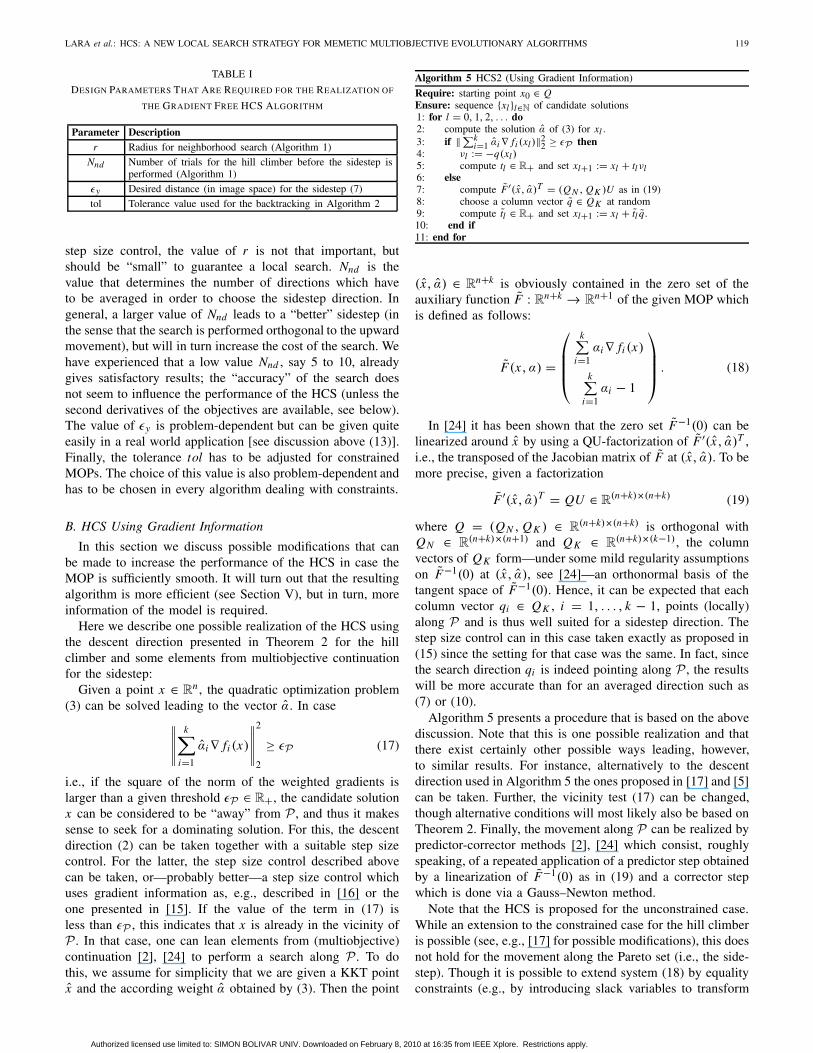
Here we present and discuss some numerical results forthe HCS as well as for the two memetic strategies in orderto demonstrate the strength of both the HCS as standalonealgorithm as well as its benefit as a local search procedurewithin a given MOEA. The MOPs we have used here arelisted in Table V. All computations have been done using theprogramming language MATLAB.3

A. HCS as a Standalone Algorithm

Since the two variants of the HCS as described in Algo-rithm 1 (which we will denote by HCS1 in this section) andin Algorithm 5 (denoted by HCS2) have no orientation in

3http://www.mathworks.com

Authorized licensed use limited to: SIMON BOLIVAR UNIV. Downloaded on February 8, 2010 at 16:35 from IEEE Xplore. Restrictions apply.

LARA et al.: HCS: A NEW LOCAL SEARCH STRATEGY FOR MEMETIC MULTIOBJECTIVE EVOLUTIONARY ALGORITHMS 127

Pareto frontNSGA�IINSGA�II�HCS1

0 20 40 60 80 100 120 140

0

20

40

60

80

100

120

f1

f 2

(a)

Pareto frontNSGA�IINSGA�II�HC2

0 20 40 60 80 100 120 140

0

20

40

60

80

100

120

f1

f 2

(b)

Pareto frontNSGA�IINSGA�II�HCS2

0 20 40 60 80 100 120 140

0

20

40

60

80

100

120

f1

f 2

(c)

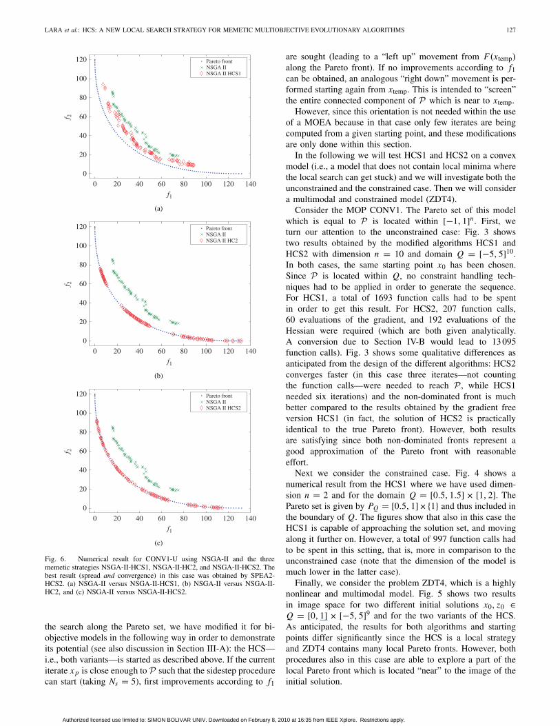
Fig. 6. Numerical result for CONV1-U using NSGA-II and the threememetic strategies NSGA-II-HCS1, NSGA-II-HC2, and NSGA-II-HCS2. Thebest result (spread and convergence) in this case was obtained by SPEA2-HCS2. (a) NSGA-II versus NSGA-II-HCS1, (b) NSGA-II versus NSGA-II-HC2, and (c) NSGA-II versus NSGA-II-HCS2.

the search along the Pareto set, we have modified it for bi-objective models in the following way in order to demonstrateits potential (see also discussion in Section III-A): the HCS—i.e., both variants—is started as described above. If the currentiterate x p is close enough to P such that the sidestep procedurecan start (taking Ns = 5), first improvements according to f1

are sought (leading to a “left up” movement from F(xtemp)along the Pareto front). If no improvements according to f1can be obtained, an analogous “right down” movement is per-formed starting again from xtemp. This is intended to “screen”the entire connected component of P which is near to xtemp.

However, since this orientation is not needed within the useof a MOEA because in that case only few iterates are beingcomputed from a given starting point, and these modificationsare only done within this section.

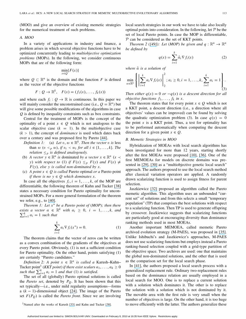
In the following we will test HCS1 and HCS2 on a convexmodel (i.e., a model that does not contain local minima wherethe local search can get stuck) and we will investigate both theunconstrained and the constrained case. Then we will considera multimodal and constrained model (ZDT4).

Consider the MOP CONV1. The Pareto set of this modelwhich is equal to P is located within [−1, 1]n. First, weturn our attention to the unconstrained case: Fig. 3 showstwo results obtained by the modified algorithms HCS1 andHCS2 with dimension n = 10 and domain Q = [−5, 5]10.In both cases, the same starting point x0 has been chosen.Since P is located within Q, no constraint handling tech-niques had to be applied in order to generate the sequence.For HCS1, a total of 1693 function calls had to be spentin order to get this result. For HCS2, 207 function calls,60 evaluations of the gradient, and 192 evaluations of theHessian were required (which are both given analytically.A conversion due to Section IV-B would lead to 13 095function calls). Fig. 3 shows some qualitative differences asanticipated from the design of the different algorithms: HCS2converges faster (in this case three iterates—not countingthe function calls—were needed to reach P , while HCS1needed six iterations) and the non-dominated front is muchbetter compared to the results obtained by the gradient freeversion HCS1 (in fact, the solution of HCS2 is practicallyidentical to the true Pareto front). However, both resultsare satisfying since both non-dominated fronts represent agood approximation of the Pareto front with reasonableeffort.

Next we consider the constrained case. Fig. 4 shows anumerical result from the HCS1 where we have used dimen-sion n = 2 and for the domain Q = [0.5, 1.5] × [1, 2]. ThePareto set is given by PQ = [0.5, 1]×{1} and thus included inthe boundary of Q. The figures show that also in this case theHCS1 is capable of approaching the solution set, and movingalong it further on. However, a total of 997 function calls hadto be spent in this setting, that is, more in comparison to theunconstrained case (note that the dimension of the model ismuch lower in the latter case).

Finally, we consider the problem ZDT4, which is a highlynonlinear and multimodal model. Fig. 5 shows two resultsin image space for two different initial solutions x0, z0 ∈Q = [0, 1] × [−5, 5]9 and for the two variants of the HCS.As anticipated, the results for both algorithms and startingpoints differ significantly since the HCS is a local strategyand ZDT4 contains many local Pareto fronts. However, bothprocedures also in this case are able to explore a part of thelocal Pareto front which is located “near” to the image of theinitial solution.

Authorized licensed use limited to: SIMON BOLIVAR UNIV. Downloaded on February 8, 2010 at 16:35 from IEEE Xplore. Restrictions apply.

128 IEEE TRANSACTIONS ON EVOLUTIONARY COMPUTATION, VOL. 14, NO. 1, FEBRUARY 2010

TABLE IX

COST OF THE HCS VARIANTS WITHIN SPEA2-HCS IN ONE

RUN ON CONV1-U (THE RUN WHICH PRODUCED THE RESULT

DISPLAYED IN FIG. 6)

Hill climber calls Sidestep calls Function callsMethod (no sidestep) (w or w/o sidestep) (total)

HCS1 7 68 2229

HC2 69 0 1262

HCS2 51 20 6145

B. HCS Coupled with a MOEA

Here we make some comparisons of the two state-of-the-art MOEAs NSGA-II and SPEA2 with their respectivehybrid variants NSGA-II-HCS and SPEA2-HCS in order todemonstrate the possible benefit of the HCS when appliedwithin a MOEA. Since we are dealing in this section withMOPs where the Pareto set is located at the boundary ofthe domain, we have used for these models a modificationof HCS2 which acts just as a hill climber. That is, the searchalong the Pareto set is not performed (the value εP is set to0). To be conform with our notations and to avoid confusions,we denote this algorithm by HC2.

In order to evaluate the performance of the algorithms wehave used the generational distance [66], the inverted genera-tional distance [9] and the two set coverage measure [70] asindicators. A brief description follows.

Denote by δi the minimum Euclidean distance from theimage F(xi ) of a given point xi , i = 1, . . . , n, to the truePareto front F(PQ). The generational distance (GD) of a set(population) P = {x1, . . . , xn} is defined as

G D = 1

n

√√√√ n∑i=1

δ2i . (27)

The inverted generational distance (IGD) is analogous to G Dbut measured from F(PQ) to F(P).

Given two finite subsets A and B of Rn the two set coverage

measure is defined as

SC(A, B)= A≺ B = |{b∈ B such that ∃a ∈ A with a ≺b}||B| .

(28)If A ≺ B = 1, it means that all the elements of B aredominated by at least one element of A. If on the other handA ≺ B = 0, it means that no element of B is dominated byany element of A. Since the two set coverage metric is notsymmetric always, both values SC(A, B) and SC(B, A) haveto be taken into account.

1) Convex Models: First we consider the convex and thusunimodal models CONV1 (k = 2 objectives) and CONV2(k = 3) which are taken from [15], and set the dimensionof the parameter space to n = 30. For both models we areinterested in the unconstrained case (where the Pareto set doesnot intersect with the boundary of the domain) and in theconstrained case. Since the Pareto set of both unconstrainedproblems (that is, for Q = R

30) is located within [−1, 1]30 wehave chosen to take the domains Qu := [−5, 5]30 and Qc =[−1, 1] × [1, 2]29 for the unconstrained and the constrained

TABLE X

PARAMETER VALUES USED FOR SPEA2 AND NSGA-II

AND THE MEMETIC STRATEGIES SPEA2-HCS AND NSGA-II-HCS

ON THE DTLZ FUNCTIONS

Parameters SPEA2-HCS NSGA-II-HCS

Npop 200 200

Na 100 —

ηc — 15

ηm — 20pc 0.9 0.9

pm 0.01 1/30

pH CS1 0.3 —

pH CS2 0.3 —

s 10 10

εy 1 5

εP 0.0001 0.0001

r 0.05 0.1

Maxiter 5 10

Nnd 5 3

tol 10−4 10−4

model, respectively. Denote the resulting models by CONV1-U and CONV1-C (analogous to CONV2).

For the realization we have used the parameter valuesdisplayed in Table VI and a budget of B = 10 000 functioncalls. B is chosen relatively low in order to obtain significantdifferences in the indicator values. Tables VII and VIII showaveraged numerical results obtained on the convex modelsusing SPEA2, NSGA-II and the corresponding memetic strate-gies. For the two cases for which we hybridize the base MOEAwith the HCS, the following observations can be made: thevalues of the Set Coverage and the GD improve when theHCS1 is used for additional local search. The values are evenmuch better when using HC2 or HCS2 for the local search(the improvement is roughly one order of magnitude). Thelatter is certainly due to the fact that we are dealing withconvex models: the gradient based search—though much morecostly than HCS1 for n = 30, see Table III—leads to greatimprovements of given initial points which do not get stuckat local solutions. Thus, the population is pulled to the “right”set at any stage of the optimization process. For IGD, theresults are not that conclusive; however, improvements can beobserved.

In Fig. 6, one result of NSGA-II and their memetic variantsis plotted which reflects the above discussion: Fig. 6(a) showsthe effect of the HCS1, i.e., better convergence and spreadthan the result of NSGA-II due to the two search directionsof HCS1. Convergence is on the other side much better inFig. 6(b) and (c) where gradient information is used. Whencomparing the latter two figures, the effects of the sidestepget visible: The spread in Fig. 6(c) is apparently better thanin Fig. 6(b), where the solutions fall into clusters.

Table IX gives an impression on the overall cost of theHCS within the search procedure. The table shows the amountof calls of the hill climber and sidestep procedures of HCSwithin SPEA2-HCS used to obtain the results in Fig. 6.HCS1 used 22% of the total budget B of SPEA2-HCS1.The relatively large amount of sidestep calls is due to the

Authorized licensed use limited to: SIMON BOLIVAR UNIV. Downloaded on February 8, 2010 at 16:35 from IEEE Xplore. Restrictions apply.

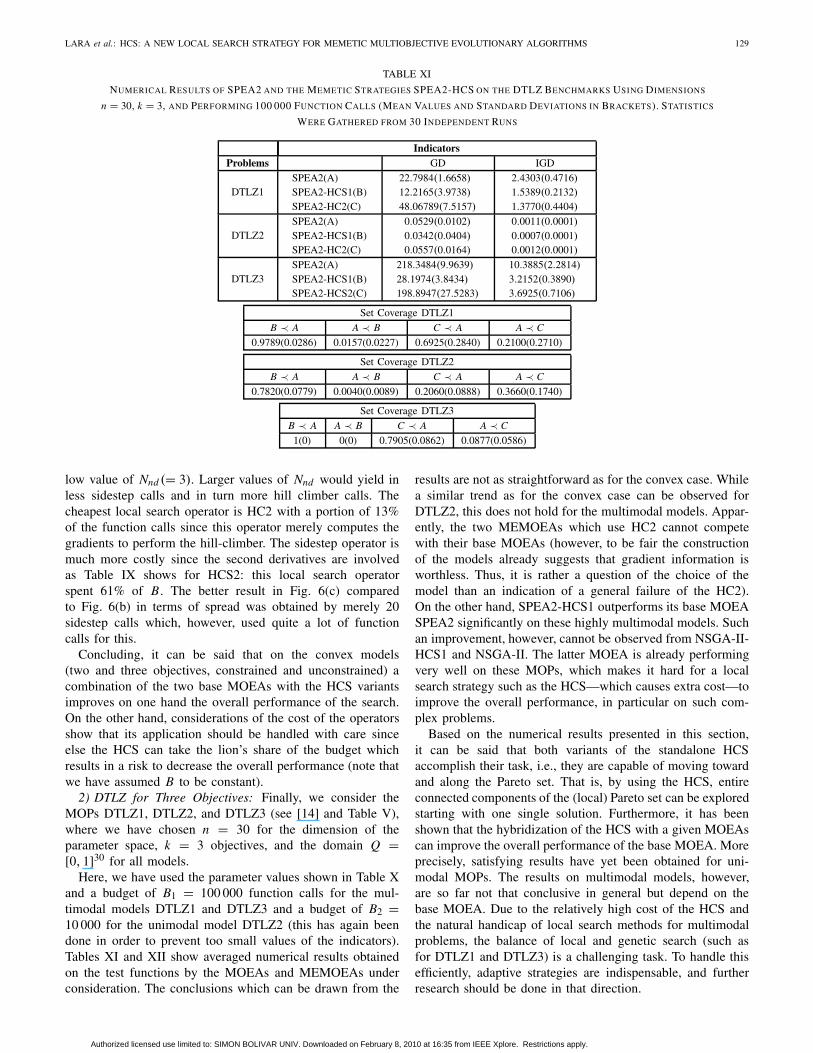
LARA et al.: HCS: A NEW LOCAL SEARCH STRATEGY FOR MEMETIC MULTIOBJECTIVE EVOLUTIONARY ALGORITHMS 129

TABLE XI

NUMERICAL RESULTS OF SPEA2 AND THE MEMETIC STRATEGIES SPEA2-HCS ON THE DTLZ BENCHMARKS USING DIMENSIONS

n = 30, k = 3, AND PERFORMING 100 000 FUNCTION CALLS (MEAN VALUES AND STANDARD DEVIATIONS IN BRACKETS). STATISTICS

WERE GATHERED FROM 30 INDEPENDENT RUNS

IndicatorsProblems GD IGD

DTLZ1SPEA2(A)SPEA2-HCS1(B)SPEA2-HC2(C)

22.7984(1.6658)

12.2165(3.9738)

48.06789(7.5157)

2.4303(0.4716)

1.5389(0.2132)

1.3770(0.4404)

DTLZ2SPEA2(A)SPEA2-HCS1(B)SPEA2-HC2(C)

0.0529(0.0102)

0.0342(0.0404)

0.0557(0.0164)

0.0011(0.0001)

0.0007(0.0001)

0.0012(0.0001)

DTLZ3SPEA2(A)SPEA2-HCS1(B)SPEA2-HCS2(C)

218.3484(9.9639)

28.1974(3.8434)

198.8947(27.5283)

10.3885(2.2814)

3.2152(0.3890)

3.6925(0.7106)

Set Coverage DTLZ1

B ≺ A A ≺ B C ≺ A A ≺ C

0.9789(0.0286) 0.0157(0.0227) 0.6925(0.2840) 0.2100(0.2710)

Set Coverage DTLZ2

B ≺ A A ≺ B C ≺ A A ≺ C

0.7820(0.0779) 0.0040(0.0089) 0.2060(0.0888) 0.3660(0.1740)

Set Coverage DTLZ3

B ≺ A A ≺ B C ≺ A A ≺ C

1(0) 0(0) 0.7905(0.0862) 0.0877(0.0586)

low value of Nnd (= 3). Larger values of Nnd would yield inless sidestep calls and in turn more hill climber calls. Thecheapest local search operator is HC2 with a portion of 13%of the function calls since this operator merely computes thegradients to perform the hill-climber. The sidestep operator ismuch more costly since the second derivatives are involvedas Table IX shows for HCS2: this local search operatorspent 61% of B . The better result in Fig. 6(c) comparedto Fig. 6(b) in terms of spread was obtained by merely 20sidestep calls which, however, used quite a lot of functioncalls for this.

Concluding, it can be said that on the convex models(two and three objectives, constrained and unconstrained) acombination of the two base MOEAs with the HCS variantsimproves on one hand the overall performance of the search.On the other hand, considerations of the cost of the operatorsshow that its application should be handled with care sinceelse the HCS can take the lion’s share of the budget whichresults in a risk to decrease the overall performance (note thatwe have assumed B to be constant).

2) DTLZ for Three Objectives: Finally, we consider theMOPs DTLZ1, DTLZ2, and DTLZ3 (see [14] and Table V),where we have chosen n = 30 for the dimension of theparameter space, k = 3 objectives, and the domain Q =[0, 1]30 for all models.

Here, we have used the parameter values shown in Table Xand a budget of B1 = 100 000 function calls for the mul-timodal models DTLZ1 and DTLZ3 and a budget of B2 =10 000 for the unimodal model DTLZ2 (this has again beendone in order to prevent too small values of the indicators).Tables XI and XII show averaged numerical results obtainedon the test functions by the MOEAs and MEMOEAs underconsideration. The conclusions which can be drawn from the

results are not as straightforward as for the convex case. Whilea similar trend as for the convex case can be observed forDTLZ2, this does not hold for the multimodal models. Appar-ently, the two MEMOEAs which use HC2 cannot competewith their base MOEAs (however, to be fair the constructionof the models already suggests that gradient information isworthless. Thus, it is rather a question of the choice of themodel than an indication of a general failure of the HC2).On the other hand, SPEA2-HCS1 outperforms its base MOEASPEA2 significantly on these highly multimodal models. Suchan improvement, however, cannot be observed from NSGA-II-HCS1 and NSGA-II. The latter MOEA is already performingvery well on these MOPs, which makes it hard for a localsearch strategy such as the HCS—which causes extra cost—toimprove the overall performance, in particular on such com-plex problems.

Based on the numerical results presented in this section,it can be said that both variants of the standalone HCSaccomplish their task, i.e., they are capable of moving towardand along the Pareto set. That is, by using the HCS, entireconnected components of the (local) Pareto set can be exploredstarting with one single solution. Furthermore, it has beenshown that the hybridization of the HCS with a given MOEAscan improve the overall performance of the base MOEA. Moreprecisely, satisfying results have yet been obtained for uni-modal MOPs. The results on multimodal models, however,are so far not that conclusive in general but depend on thebase MOEA. Due to the relatively high cost of the HCS andthe natural handicap of local search methods for multimodalproblems, the balance of local and genetic search (such asfor DTLZ1 and DTLZ3) is a challenging task. To handle thisefficiently, adaptive strategies are indispensable, and furtherresearch should be done in that direction.

Authorized licensed use limited to: SIMON BOLIVAR UNIV. Downloaded on February 8, 2010 at 16:35 from IEEE Xplore. Restrictions apply.

130 IEEE TRANSACTIONS ON EVOLUTIONARY COMPUTATION, VOL. 14, NO. 1, FEBRUARY 2010

TABLE XII

NUMERICAL RESULTS OF NSGA-II AND THE MEMETIC STRATEGIES NSGA-II-HCS ON THE DTLZ BENCHMARKS USING DIMENSIONS

n = 30, k = 3, AND PERFORMING 100 000 FUNCTION CALLS (MEAN VALUES AND STANDARD DEVIATIONS IN BRACKETS). STATISTICS

WERE GATHERED FROM 30 INDEPENDENT RUNS

IndicatorsProblems GD IGD

DTLZ1NSGA-II(A)NSGA-II-HCS1(B)NSGA-II-HC2(C)

8.5024(1.2081)

10.4444(1.1505)

18.1555(4.6705)

1.5998(0.1530)

1.6856(0.2202)

1.0096(0.1899)

DTLZ2NSGA-II(A)NSGA-II-HCS1(B)NSGA-II-HC2(C)

0.0363(0.0041)

0.0293(0.0033)

0.0097(0.0039)

0.0022(0.0002)

0.0018(0.0001)

0.0005(0)

DTLZ3NSGA-II(A)NSGA-II-HCS1(B)NSGA-II-HC2(C)

17.6126(3.5630)

16.9381(2.9723)

24.6485(3.6724)

3.2696(0.7721)

2.9951(0.6861)

2.5127(0.4320)

Set Coverage DTLZ1

B ≺ A A ≺ B C ≺ A A ≺ C

0.1610(0.1376) 0.6035(0.2565) 0.4885(0.1354) 0.3960(0.1627)

Set Coverage DTLZ2

B ≺ A A ≺ B C ≺ A A ≺ C

0.7125(0.1869) 0.1235(0.0790) 0.9715(0.0284) 0.0105(0.0116)

Set Coverage DTLZ3

B ≺ A A ≺ B C ≺ A A ≺ C

0.5010(0.3365) 0.3965(0.3243) 0.4435(0.3225) 0.4550(0.2857)

VI. CONCLUSION AND FUTURE WORK

We have proposed a novel point-wise iterative search pro-cedure, called the HCS, which is designed for the local searchof a given MOP. The HCS is intended to be capable to movingboth toward and along the set of (local) Pareto points, depend-ing on the location of the current iterate. We have proposedtwo variants of the HCS, a gradient free version (HCS1) anda version that exploits gradient information (HCS2). Bothalgorithms can be used as standalone algorithms to exploreparts of the Pareto set starting with one single solution andare able to handle constraints of the model to some extend.Further, we have addressed the problem of integrating theHCS into a given MOEA in order to obtain a novel memeticstrategy. As examples, we have proposed the two algorithms(or family of algorithms) SPEA2-HCS and NSGA-II-HCSwhich are derived from SPEA2 and NSGA-II, respectively.Finally, we have presented some numerical results indicatingthe efficiency of the HCS as a standalone algorithm and itsbenefit when beeing integrated into a MOEA. More precisely,the results of SPEA2-HCS and NSGA-II-HCS show that thecombination as proposed here is advantageous in many cases.However, it has to be mentioned that for this the designparameters of the HCS and the balance between local andgenetic search have to be chosen properly, which is so far notdone in an adaptive manner.

For future work, there are some interesting topics thatcan be addressed to advance the present work. In the firstplace, there is probably the design of an adaptive strategy tochoose the design parameters as discussed above. Further, thecoupling of local and global search could be improved. Forthis, an adaptive choice of the local search probability wouldbe desirable (as done in [8]), or other techniques to reduce thecomputational complexity, e.g., by involving the information

of the current population into the HCS. Another interestingtopic would be to develop a version of HCS2 that can moveefficiently along the Pareto set even if it is contained in theboundary of the domain which would allow for a more generaluse of the algorithm. Finally, it is conceivable to apply andadvance the standalone HCS to other contexts. Areas whichseem to be promising for that are numerical path-following(see [54] for a first study) or dynamic MOO.

REFERENCES

[1] S. F. Adra, I. Griffin, and P. J. Fleming, “Hybrid multiobjective geneticalgorithm with a new adaptive local search process,” in Proc. GeneticEvol. Comput. Conf. (GECCO ’05), vol. 1. New York: ACM, Jun. 2005,pp. 1009–1010.

[2] E. L. Allgower and K. Georg, Numerical Continuation Methods. 1st ed.New York: Springer-Verlag, 1990.

[3] L. Armijo, “Minimization of functions having Lipschitz-continuous firstpartial derivatives,” Pacific J. Math., vol. 16, no. 1, pp. 1–3, 1966.

[4] N. K. Bambha, S. S. Bhattacharyya, J. Teich, and E. Zitzler, “Systematicintegration of parameterized local search into evolutionary algorithms,”IEEE Trans. Evol. Comput., vol. 8, no. 2, pp. 137–155, Apr. 2004.

[5] P. A. N. Bosman and E. D. de Jong, “Exploiting gradient informationin numerical multiobjective evolutionary optimization,” in Proc. GeneticEvol. Comput. Conf. (GECCO ’05), vol. 1. New York: ACM, Jun. 2005,pp. 755–762.

[6] J. Branke and S. Mostaghim, “About selecting the personal best inmultiobjective particle swarm optimization,” in Proc. 9th Int. Conf. Par-allel Problem Solving from Nature (PPSN), LNCS vol. 4193. Reykjavik,Iceland: Springer-Verlag, Sep. 2006, pp. 523–532.

[7] M. Brown and R. E. Smith, “Directed multiobjective optimisation,” Int.J. Comput., Syst. Signals, vol. 6, no. 1, pp. 3–17, 2005.

[8] A. Caponio and F. Neri, “Integrating cross-dominance adaption inmultiobjective memetic algorithms,” Multiobjective Memetic Algorithms,SCI vol. 171. New York: Springer-Verlag, 2009, pp. 325–351.

[9] C. A. Coello Coello and N. Cruz Cortés, “Solving multiobjectiveoptimization problems using an artificial immune system,” GeneticProgramming Evolvable Mach., vol. 6, no. 2, pp. 163–190, Jun. 2005.

[10] C. A. Coello Coello, G. B. Lamont, and D. A. Van Veldhuizen,Evolutionary Algorithms for Solving Multiobjective Problems. 2nd ed.New York: Springer-Verlag, Sep. 2007.

Authorized licensed use limited to: SIMON BOLIVAR UNIV. Downloaded on February 8, 2010 at 16:35 from IEEE Xplore. Restrictions apply.

LARA et al.: HCS: A NEW LOCAL SEARCH STRATEGY FOR MEMETIC MULTIOBJECTIVE EVOLUTIONARY ALGORITHMS 131

[11] I. Das and J. Dennis, “Normal-boundary intersection: A new methodfor generating the Pareto surface in nonlinear multicriteria optimizationproblems,” SIAM J. Optimization, vol. 8, no. 3, pp. 631–657, 1998.

[12] K. Deb, Multiobjective Optimization Using Evolutionary Algorithms.1st ed. Chichester, U.K.: Wiley, 2001.

[13] K. Deb, A. Pratap, S. Agarwal, and T. Meyarivan, “A fast and elitistmultiobjective genetic algorithm: NSGA–II,” IEEE Trans. Evol. Com-put., vol. 6, no. 2, pp. 182–197, Apr. 2002.

[14] K. Deb, L. Thiele, M. Laumanns, and E. Zitzler, “Scalable test problemsfor evolutionary multiobjective optimization,” Evolutionary Multiob-jective Optimization. Theoretical Advances and Applications, 1st ed.New York: Springer-Verlag, 2005, ch. 6, pp. 105–145.

[15] M. Dellnitz, O. Schütze, and T. Hestermeyer, “Covering Pareto setsby multilevel subdivision techniques,” J. Optimization Theory Applicat.,vol. 124, no. 1, pp. 113–155, 2005.

[16] J. E. Dennis and R. B. Schnabel, Numerical Methods for UnconstrainedOptimization and Nonlinear Equations. 1st ed. Englewood Cliffs, NJ:Prentice-Hall, 1983.

[17] J. Fliege and B. Fux Svaiter, “Steepest descent methods for multicri-teria optimization,” Math. Methods Operations Res., vol. 51, no. 3,pp. 479–494, 2000.

[18] F. Glover and M. Laguna, Tabu Search. 1st ed. New York: Springer-Verlag, 1997.

[19] T. Goel and K. Deb, “Hybrid methods for multiobjective evolutionaryalgorithms,” in Proc. 4th Asia-Pacific Conf. Simulated Evol. Learning(SEAL ’02), vol. 1. Singapore, Nov. 2002, pp. 188–192, Nanyang Tech.Univ.

[20] A. Griewank, “Evaluating derivatives: Principles and techniques ofalgorithmic diffierentiation,” Number 19 Frontiers Appl. Math., 1st ed.Philadelphia, PA: SIAM, 2000.

[21] N. Hansen and A. Ostermeier, “Completely derandomized self-adaptation in evolution strategies,” Evol. Comput., vol. 9, no. 2,pp. 159–195, Summer 2001.

[22] K. Harada, J. Sakuma, and S. Kobayashi, “Uniform sampling of localpareto-optimal solution curves by pareto path following and its appli-cations in multiobjective GA,” in Proc. Genetic Evol. Comput. Conf.(GECCO ’07), vol. 1. London, U.K.: ACM, Jul. 2007, pp. 813–820.

[23] W. E. Hart, “Adaptive global optimization with local search,” Ph.D.thesis, Dept. Comput. Sci. Eng., Univ. California, San Diego, CA, 1994.

[24] C. Hillermeier, Nonlinear Multiobjective Optimization a GeneralizedHomotopy Approach. 1st ed. Cambridge, MA: Birkhäuser, 2001.

[25] X. Hu, Z. Huang, and Z. Wang, “Hybridization of the multiobjectiveevolutionary algorithms and the gradient based algorithms,” in Proc.Congr. Evol. Comput. 2003 (CEC ’03), vol. 2. Canberra, Australia:IEEE Press, Dec. 2003, pp. 870–877.

[26] C. Igel, N. Hansen, and S. Roth, “Covariance matrix adaptation formultiobjective optimization,” Evol. Comput., vol. 15, no. 1, pp. 1–28,Spring 2007.

[27] A. W. Iorio and X. Li, “Solving rotated multiobjective optimization prob-lems using diffierential evolution,” in Proc. Advances Artificial Intell. (AI’04), LNAI vol. 3339. New York: Springer-Verlag, pp. 861–872.

[28] A. W. Iorio and X. Li, “Rotated problems and rotationally invariantcrossover in evolutionary multiobjective optimization,” Int. J. Comput.Intell. Applicat., vol. 7, no. 2, pp. 149–186, 2008.

[29] H. Ishibuchi and T. Murata, “Multiobjective genetic local search algo-rithm,” in Proc. Int. Conf. Evol. Comput. 1996, Nagoya, Japan: IEEEPress, pp. 119–124.

[30] H. Ishibuchi and T. Murata, “A multiobjective genetic local searchalgorithm and its application to flowshop scheduling,” IEEE Trans. Syst.,Man, Cybern. Part C: Applicat. Rev., vol. 28, no. 3, pp. 392–403,Aug. 1998.

[31] H. Ishibuchi, T. Yoshida, and T. Murata, “Balance between geneticsearch and local search in memetic algorithms for multiobjective permu-tation flowshop scheduling,” IEEE Trans. Evol. Comput., vol. 7, no. 2,pp. 204–223, Apr. 2003.

[32] A. Jaszkiewicz, “Do multiple-objective metaheuristics deliver on theirpromises? A computational experiment on the set-covering problem,”IEEE Trans. Evol. Comput., vol. 7, no. 2, pp. 133–143, Apr. 2003.

[33] W. E. Karush, “Minima of functions of several variables with inequalitiesas side conditions,” Ph.D. thesis, Dept. Math., Univ. Chicago, Chicago,IL, 1939.

[34] S. Kirkpatrick, C. D. Gelatt, and M. P. Vecchi, “Optimization bysimulated annealing,” New Ser. Sci., vol. 220, no. 4598, pp. 671–680,1983.

[35] J. Knowles and D. Corne, “M-PAES: A memetic algorithm for mul-tiobjective optimization,” in Proc. Congr. Evol. Comput. 2000, vol. 1.Piscataway, NJ: IEEE Service Center, Jul. 2000, pp. 325–332.

[36] J. Knowles and D. Corne, “Memetic algorithms for multiobjectiveoptimization: Issues, methods and prospects,” Recent Advances inMemetic Algorithms, SFSC vol. 166. New York: Springer-Verlag, 2005,pp. 313–352.

[37] N. Krasnogor, “Studies on the theory and design space of memeticalgorithms,” Ph.D. thesis, Faculty Comput., Eng. Math. Sci., Univ. WestEngland, Bristol, U.K., 2002.

[38] H. Kuhn and A. Tucker, “Nonlinear programming,” in Proc. 2ndBerkeley Symp. Math. Statist. Probability, 1951, pp. 481–492.

[39] M. Lozano, F. Herrera, N. Krasnogor, and D. Molina, “Real-codedmemetic algorithms with crossover hill-climbing,” Evol. Comput.,vol. 12, no. 3, pp. 273–302, 2004.

[40] K. Miettinen, Nonlinear Multiobjective Optimization. 1st ed. Boston,MA: Kluwer, 1999.

[41] T. Murata, S. Kaige, and H. Ishibuchi, “Generalization of dominancerelation-based replacement rules for memetic EMO algorithms,” inProc. Part I Genetic Evol. Comput. (GECCO ’03), LNCS vol. 2723.New York: Springer-Verlag, Jul. 2003 pp. 1234–1245.

[42] J. Nocedal and S. J. Wright, “Numerical optimization,” Springer Seriesin Operations Research, New York: Springer-Verlag, 1999.

[43] U.-M. O’Reilly and F. Oppacher, “Hybridized crossover-based searchtechniques for program discovery,” in Proc. World Conf. Evol. Comput.1995, vol. 2. Perth, Australia: IEEE Press, pp. 573–578.

[44] V. Pareto, Manual of Political Economy. 1st ed. New York: MacMillan,1971.

[45] S. Poles, E. Rigoni, and T. Robic, “MOGA-II performance on noisy opti-mization problems,” in Proc. Int. Conf. Bioinspired Optimization Meth-ods Applicat. (BIOMA ’04), Ljubljana, Slovenia, Oct. 2004, pp. 51–62.

[46] E. Rigoni and S. Poles, “NBI and MOGA-II, two complemen-tary algorithms for multiobjective optimization,” Practical Approachesto Multiobjective Optimization, Dagstuhl, Germany: InternationalesBegegnungs-und Forschungszentrum für Informatik (IBFI), 2005,pp. 1–22.

[47] H. H. Rosenbrock, “An automatic method for finding the greatest orleast value of a function,” Comput. J., vol. 3, no. 3, pp. 175–184, 1960.

[48] H. Satoh, M. Yamamura, and S. Kobayashi, “Minimal generation gapmodel for gas considering both exploration and exploitation,” in Proc.IIZUKA ’96, vol. 2. Fukuoka, Japan, 1996, pp. 494–497.

[49] S. Schäffler, R. Schultz, and K. Weinzierl, “A stochastic method for thesolution of unconstrained vector optimization problems,” J. OptimizationTheory Applicat., vol. 114, no. 1, pp. 209–222, 2002.

[50] O. Schütze, M. Laumanns, E. Tantar, C. A. Coello Coello, and E.-G.Talbi, “Convergence of stochastic search algorithms to gap-free Paretofront approximations,” in Proc. Genetic Evol. Comput. Conf. (GECCO’07), vol. 1. London, U.K.: ACM, Jul. 2007, pp. 892–899.

[51] O. Schütze, G. Sanchez, and C. A. Coello Coello, “A new memeticstrategy for the numerical treatment of multiobjective optimizationproblems,” in Proc. Genetic Evol. Comput. Conf. (GECCO ’08), Atlanta,GA: ACM, Jul. 2008, pp. 705–712.

[52] O. Schütze, “Set oriented methods for global optimization,” Ph.D.thesis, Fakultät für Elektrotechnik, Informatik und Mathematik, Univ.Paderborn, Paderborn, Germany, 2004. Available: http://ubdata.uni-paderborn.de/ediss/17/2004/schuetze/

[53] O. Schütze, C. A. Coello Coello, S. Mostaghim, E.-G. Talbi, andM. Dellnitz, “Hybridizing evolutionary strategies with continuationmethods for solving multiobjective problems,” Eng. Optimization,vol. 40, no. 5, pp. 383–402, May 2008.

[54] O. Schütze, A. Lara, and C. A. Coello Coello, “Evolutionary continua-tion methods for optimization problems,” in Proc. Genetic Evol. Comput.Conf. (GECCO ’09), Jul. 8–12, 2009, pp. 651–658.

[55] O. Schütze, S. Mostaghim, M. Dellnitz, and J. Teich, “Covering paretosets by multilevel evolutionary subdivision techniques,” in Proc. 2nd Int.Conf. Evol. Multicriterion Optimization (EMO ’03), LNCS. vol. 2632.Faro, Portugal: Springer-Verlag, Apr. 2003, pp. 118–132.

[56] O. Schütze, E.-G. Talbi, C. A. Coello Coello, L. V. Santana-Quintero,and G. Toscano Pulido, “A memetic PSO algorithm for scalar optimiza-tion problems,” in Proc. IEEE Swarm Intell. Symp. (SIS ’07), Honolulu,HI: IEEE Press, Apr. 2007, pp. 128–134.

[57] K. Sindhya, K. Deb, and K. Miettinen, “A local search based evo-lutionary multiobjective optimization approach for fast and accurateconvergence,” in Proc. Parallel Problem Solving from Nature–PPSNX, LNCS vol. 5199. Dortmund, Germany: Springer-Verlag, Sep. 2008,pp. 815–824.

[58] A. Sinha, Y.-P. Chen, and D. E. Goldberg, “Designing efficient geneticand evolutionary algorithm hybrids,” Recent Advances Memetic Algo-rithms, SFSC vol. 166. New York: Springer-Verlag, 2005, pp. 259–288.

Authorized licensed use limited to: SIMON BOLIVAR UNIV. Downloaded on February 8, 2010 at 16:35 from IEEE Xplore. Restrictions apply.

132 IEEE TRANSACTIONS ON EVOLUTIONARY COMPUTATION, VOL. 14, NO. 1, FEBRUARY 2010

[59] J. E. Smith and T. C. Fogarty, “Operator and parameter adaption ingenetic algorithms,” Soft Comput., vol. 1, no. 2, pp. 81–87, 1997.

[60] O. Soliman, L. T. Bui, and H. Abbass, “A memetic coevolutionary multi-objective differential evolution algorithm,” Multiobjective Memetic Algo-rithms, SCI vol. 171. New York: Springer-Verlag, 2009, pp. 325–351.

[61] B. Suman, “Study of simulated annealing based algorithms for multiob-jective optimization of a constrained problem,” Comput. Chemical Eng.,vol. 28, no. 9, pp. 1849–1871, Aug. 2004.

[62] M. Vasile, “A behavior-based meta-heuristic for robust global trajec-tory optimization,” in Proc. IEEE Congr. Evol. Comput. (CEC ’07),Singapore: IEEE Press, pp. 494–497.

[63] M. Vasile, “Hybrid behavioral-based multiobjective space trajectoryoptimization,” Multiobjective Memetic Algorithms, SCI vol. 171.New York: Springer-Verlag, 2009, pp. 231–254.

[64] M. Vasile and M. Locatelli, “A hybrid multiagent approach for globaltrajectory optimization,” J. Global Optimization, vol. 44, no. 4, pp. 461–479, Aug. 2009.

[65] M. Vasile and C. Maddock, “Design of optimal spacecraft-asteroidformations through a hybrid global optimization approach,” Int. J.Intelligent Comput. Cybern., vol. 1, no. 2, pp. 239–268, 2008.

[66] D. A. Van Veldhuizen, “Multiobjective evolutionary algorithms: Clas-sifications, analyses, and new innovations,” Ph.D. thesis, Dept Elect.Comput. Eng., Graduate School Eng., Air Force Inst. Technol., Wright-Patterson AFB, Dayton, OH, May 1999.

[67] Y. Wang, Z. Cai, G. Guo, and Y. Zhou, “Multiobjective optimizationand hybrid evolutionary algorithm to solve constrained optimizationproblems,” IEEE Trans. Syst., Man Cybern. Part B–Cybern., vol. 37,no. 3, pp. 560–575, Jun. 2007.

[68] E. F. Wanner, F. G. Guimaraes, R. H. C. Takahashi, and P. J. Fleming,“A quadratic approximation-based local search procedure for multiob-jective genetic algorithms,” in Proc. IEEE Congr. Evol. Comput. (CEC’06), Vancouver, BC, Canada: IEEE, Jul. 2006, pp. 3361–3368.

[69] Y. Yin, T. Okabe, and B. Sendhoff, “Adapting weighted aggrega-tion for multiobjective evolution strategies,” in Proc. 1st Int. Conf.Proc. Evol. Multicriterion Optimization (EMO ’01), LNCS vol. 1993.New York: Springer-Verlag, pp. 96–110.

[70] E. Zitzler, K. Deb, and L. Thiele, “Comparison of multiobjectiveevolutionary algorithms: Empirical results,” Evol. Comput., vol. 8, no. 2,pp. 173–195, Jun. 2000.

[71] E. Zitzler, M. Laumanns, and L. Thiele, “SPEA2: Improving thestrength pareto evolutionary algorithm,” in Proc. Evol. Methods Design,Optimization Control Applicat. Ind. Problems (EUROGEN ’01), Athens,Greece, 2002, pp. 95–100.

[72] E. Zitzler and L. Thiele, “Multiobjective evolutionary algorithms:A comparative case study and the strength pareto approach,” IEEETrans. Evol. Comput., vol. 3, no. 4, pp. 257–271, Nov. 1999.

Adriana Lara received the B.Sc. degree in physicsand mathematics in 2001 from the National Poly-technic Institute of México. In 2003, she receivedthe M.Sc. degree in electrical and computer engi-neering, from the Departamento de Computación,Centro de Investigación y de Estudios Avanzados-Instituto Politécnico Nacional (CINVESTAV-IPN),México City, Mexico. She is currently pursuing thePh.D. degree in computer sciences at CINVESTAV-IPN.

Earlier, she was an Associate Professor at theNational Polytechnic Institute of México, México City. Her main researchinterests include multiobjective optimization, gradient based techniques, andhybrid algorithms.

Gustavo A. Sánchez received the B.S. degree in1994 from the University of Metz, France, and theM.S. degree in 2004 from Simon Bolivar University,Caracas, Venezuela, both in systems engineering.

He was a Control Engineer for several oil com-panies. He is currently an Associate Professor inthe Department of Process and Systems, SimonBolivar University, Caracas. His research interestsinclude control systems, multiobjective optimizationand evolutionary algorithms.

Carlos A. Coello Coello (M’99–SM’04) receivedthe B.Sc. degree in civil engineering from the Uni-versidad Autónoma de Chiapas, México, and theM.Sc. and Ph.D. degrees in computer science fromTulane University, New Orleans, LA, in 1991, 1993,and 1996, respectively.

He is currently a Professor (CINVESTAV-3-DResearcher) at the Department of Computación,Centro de Investigación y de Estudios Avanzados-Instituto Politécnico Nacional (CINVESTAV-IPN),México City, Mexico. He has authored and co-

authored over 180 technical papers and several book chapters. He has alsoco-authored the book Evolutionary Algorithms for Solving MultiobjectiveProblems (2nd edition, Springer, 2007). His major research interests areevolutionary multiobjective optimization and constraint-handling techniquesfor evolutionary algorithms.

Dr. Coello received the 2007 National Research Award from the MexicanAcademy of Sciences in the area of exact sciences. He is an Associate Editorof the IEEE TRANSACTIONS ON EVOLUTIONARY COMPUTATION and serveson the Editorial Board of seven other international journals. He also chairsthe IEEE Computationally Intelligent Society Task Force on MultiobjectiveEvolutionary Algorithms. He is a member of the ACM, Sigma Xi, and theMexican Academy of Sciences.

Oliver Schütze received the Diploma in mathe-matics from the University of Bayreuth, Germany,and the Ph.D. degree in natural sciences from theUniversity of Paderborn, Germany, in 1999 and2004, respectively.

He is currently a Professor (CINVESTAV-2CResearcher) at the Departamento de Computación,Centro de Investigación y de Estudios Avanzados-Instituto Politécnico Nacional (CINVESTAV-IPN),México City, Mexico.

Authorized licensed use limited to: SIMON BOLIVAR UNIV. Downloaded on February 8, 2010 at 16:35 from IEEE Xplore. Restrictions apply.