Evaluating Center-Seeking and Initialization Bias: The case of Particle Swarm and Gravitational...

Evaluating Center-Seeking and Initialization Bias:The case of Particle Swarm and Gravitational

Search Algorithms (Extended Version)Mohsen Davarynejad∗†, Jan van den Berg∗ and Jafar Rezaei∗

∗Faculty of Technology, Policy and Management, Delft University of Technology,Jaffalaan 5, Delft 2628BX, The Netherlands

Email: {M.Davarynejad; J.vandenBerg; J.Rezaei}@tudelft.nl†Department of Radiation Oncology, Erasmus Medical Center—Daniel den Hoed Cancer Center,

Groene Hilledijk 301, Rotterdam 3075EA, The Netherlands

Abstract—Complex optimization problems that cannot besolved using exhaustive search require efficient search meta-heuristics to find optimal solutions. In practice, metaheuristicssuffer from various types of search bias, the understandingof which is of crucial importance, as it directly pertinent tothe problem of making the best possible selection of solvers.Two metrics are introduced in this study: one for measuringcenter-seeking bias (CSB) and one for initialization region bias(IRB). The former is based on “ξ-center offset”, an alternativeto “center offset”, which is a common but, as will be shown,inadequate approach to analyzing the center-seeking behaviorof algorithms. The latter is proposed on the grounds of “regionscaling”. The introduced metrics are used to evaluate the biasof three algorithms while running on a test bed of optimizationproblems having their optimal solution at, or near, the center ofthe search space. The most prominent finding of this paper isconsiderable CSB and IRB in the gravitational search algorithm(GSA). In addition, a partial solution to the center-seeking andinitialization region bias of GSA is proposed by introducing a“mass-dispersed” version of GSA, mdGSA. The performance ofmdGSA, which promotes the global search capability of GSA,is verified using the same mathematical optimization problemin addition to a gene regulatory network system parameteridentification, the results of which demonstrate the capabilitiesof the mdGSA in solving real-world optimization problems.

I. I NTRODUCTION

Consider asearch scenarioin a finite continuous searchspaceE ⊂ X defined by

E =

D⊗

d=1

[Ldx,U

dx], (1)

with the objective of locatingx∗ ∈ E, wheref(x∗) is theextremum of a functionf(x) : E → IR, and whereLd

x andUdx are respectively the lower and upper bound of the search

domain at dimensiond. Optimization problems are to be foundin such diverse arenas as engineering, business, medicine,etc. [5]. Without loss of generality, a minimization problemis considered here.

In contrast to exhaustive search which looks into every entryin the search space,metaheuristics[23] are strategies whichguide the search process iteratively, in many cases by making

a trade-off between exploration and exploitation. This is animportant notion when it comes to allocating scarce resourcesto the exploration of new possibilities and the exploitation ofold certainties.

Nature has been the original inspiration for many typesof metaheuristics. Two distinct classes of nature-inspired op-timization algorithms are evolutionary algorithms (EA), andswarm intelligence (SI)-based algorithms. Some popular mem-bers of the former class are genetic algorithm (GA) [25] anddifferential evolution (DE) [46], [57]. Successful instancesof swarm intelligence-based algorithms are particle swarmoptimization (PSO) [28] and the gravitational search algorithm(GSA) [47].

Arguments for allowing bias in the search methods statethat a learning system may be shaped towards the impor-tant features of a problem [60]. So when more informationabout the solution becomes available then the user may takeadvantage of specific types of search bias. However generalpurpose optimizers make no assumption on the problem atstake. Studying the properties of these algorithms, it turns outthat some of them suffer from a specific search bias [12],[36]: they tend to perform best when the optimum is locatedat or near the center of the search space. Consequently, whento comparing the quality of the solutions found by a set ofmetaheuristics on a series of benchmark problems with optimalsolution near the center of the search space, the comparisonbecomes unfair.

To remedy this unfairness, the so-calledcenter offset(CO) [37] approach was proposed which changes the bordersof the search space in such a way that the optimal solution isno longer located in the center of the search space. Basically,the CO approach changes the search space of the originalproblem by reducing it on one side and expanding it at theother. When comparing a set of algorithmsqualitatively, thecomparison is valid since interference tends to be reducedwhen all the contenders are submitted to the same set ofbenchmarks, no matter if the shifting has introduced somedegree of increase/decrease in the complexity of the search.Our goal, here, is to supplement the comparison by developing

quantitativemeasures that can assist the observer in evaluationof the “degree” of CSB of a certain search algorithm. Quan-titative measures are succinct and are the preferred disclosureform, not only for a) a comparison of the degree of CSB ina set of search algorithms, but also when the task is b) toexamine if a single search algorithm has any CSB at all.

On the basis of these observations, we decided to examinegeneric methods for evaluating the search bias of differentalgorithms. In this paper, we limit ourselves to two metrics;one for measuring center-seeking bias, and one for initializa-tion bias. These metrics are used to evaluate the behavioralbias of several algorithms related to swarm optimization andgravitational search.

Section II-A presents the center offset (CO) approach (in-troduced in [1]) to capture the center-seeking behavior ofpopulation based algorithms. Then proceeds by arguing thatCO is not a reliable test. Then in Section II-B a solution forthe unknown change in problem complexity as a result ofusing CO approach when changing the center of the searchspace is reported and a metric to measure the CS behaviorof population based optimization techniques is presented.Ametric to measure initialization region bias is then presentedin Section III. In Section IV-A and IV-B PSO and GSAare briefly summarized. Next, in Section IV-C, the searchbias of the GSA in favor of center of the search space isconceptualized. Then we present a solution to partially dilutethe search bias of GSA. In Section V We have analyzed thesearch behavior of the studied contenders by setting up anumber of tests similar to those proposed by Angeline [1] ona set of several widely used numerical benchmark problemswith various optimization characteristics. In addition tothestudied benchmark problems, a gene regulatory network modelidentification problem is studied to asses the performance ofthe GSA and the presented modification of GSA. Section VIpresents discussions and provides a framework that enablesafair comparison of optimization heuristics. The last sectionhighlights conclusions and provides suggestions for futureresearch.

II. A METRIC FOR MEASURING CENTER-SEEKING BIAS

A. Understanding the assumptions underlying center offset

According to theNo Free Lunchtheorem [62], all learningsystems will expose equal performance over all possible costfunctions. This implies that, in order to efficiently solve anoptimization problem, they should be tailored to the salientproblem-specific characteristics. Where there is no availableinformation on the problem at hand, as with various real-worldapplications, some search biases known to us are not often ofservice. Such biases include center-seeking (CS) behaviorandinitialization region bias (IRB), the foci of this study.

When comparing nature-inspired metaheuristic algorithms,a symmetric search space can be misleading when the optimalsolution is located at, or near, the center of the search space. Insuch a case, one must account for CS behavior in order to drawvalid conclusions from an experiment [8]. One attempt to dealwith CS bias is calledcenter offset(CO). This is a common

0 0.05 0.1 0.15 0.2 0.25 0.3 0.35−1

−0.5

0

0.5

1

1.5

Design space, x

f(x)

a)

0 0.05 0.1 0.15 0.2 0.25 0.3 0.35−1

−0.5

0

0.5

1

1.5

Design space, x

f(x−.05)

b)

Optimal Solution

Fig. 1: Change in complexity as a result of CO. a) The originalfunction, b) The transformed function.

approach to negating the centrist bias of an optimizationalgorithm [3]. The underlying assumption of CO is that thecomplexity of a problem does not change as a result of movingthe optimal solution from the center of the search space; thisis an assumption that is discussed in greater detail below.

When applying CO, the optimization problemf(x) ischanged tof(x − C) whereC is the location of the newcenter. CO is equivalent to expanding the search space fromone side, for each dimensiond, and to shrinking it on the otherside, without changing the distance‖Ud

x − Ldx‖ between the

lower boundLdx and the upper boundUd

x . When the objectiveof a test is to measure the search bias of an algorithm, CO is ofnot of any use. This is because a change in the complexity ofa problem is not explicitly controlled: without any additionalinformation, the complexity of the problem might increased,decreased, or even remained the same. As a consequence, anyobserved difference in the performance of an algorithm cannot,to any degree of certainty, be associated with the CS bias ofthe algorithm; it may also have been caused by an (unknown)change in the problem complexity.

Figure 1 shows an example of an increase in problemcomplexity (due to an increase in the number of local optimalsolutions) as a result of shifting the search window when theobjective is to locate the minimum of the following function:

f(x) = 10 (x− 0.2)2+ sin(

π

x), 0.1 ≤ x ≤ 0.3. (2)

In this case, due to an increased problem complexity,the average performance ofany metaheuristic is expected todeteriorate whether or not the algorithm possesses CS bias.Consequently no hypothesis can be made on the CS behaviorof an optimization algorithm.

Assuming we know that the problem complexity decreases,some decision making around CS behavior becomes possible.If a certain algorithm shows a better performance, one can

conclude that this algorithm has no observable CS bias, sincewe would otherwise have observed a deterioration in itsperformance, i.e., a deterioration in the best found fitnessduring optimization. Figure 2 summarizes the concerns thatneed to be addressed before drawing any conclusion regardingthe outcome of the standard CO test, which provides anargument in favor of searching for an alternative CO-approach,in which it is known that the problem complexity alwaysdecreases. In this study, theξ-CO approach is introduced toremove the uncertainties on change in problem complexity(dashed arrows in Figure 2).

In ξ-CO, the search space is downsized asymmetrically, as aresult of which the problem complexity always decreases andthe algorithm is expected to locate a near optimal solutionmore quickly and with greater precision if there is no center-seeking bias. This makes it possible to test the hypotheseson CS behavior of an optimization algorithm considering abenchmark problem with (i) a symmetric search space and(ii ) the optimal solution near the center of the search space.Let us assume thatLd

x = −Udx and thatUd

x > 0, as is the casefor most of the problems studied here. Inξ-CO, the searchspace is downsized asymmetrically by modifying the lowerbound of the search spaceLd

x according to

Ldx = Ld

x +ξ

100× ||Ud

x − Ldx||

2, (3)

whereξ ∈ [ξL, ξU ] is the percentage of downsizing the searchspace and whereξL andξU are the predefined lower and upperbound ofξ, respectively.

Observe that CO is only worthwhile for optimization prob-lems whose support extends outside of the initial boundaryconstraints. With the proposedξ-CO approach this shortcom-ing does not arise.

B. A metric for center-seeking bias

After identifying ξ-CO as an appropriate approach foranalyzing CS behavior of optimization heuristics, there isstilla need to quantify the observations on the CS bias behavior,i.e., a metric is needed. By executing a series of runs whengradually increasing, with a predefined step size ofξs, thepercentageξ of downsizing the search space from a lower limitξL to an upper limitξU , one can measure the best-fitness eachoptimization algorithm can attain. Because randomly choseninitializations affect the outcome, experiments under equalconditions are usually repeated several times, sayrf time,yielding a data of the form

(

ξ, f ξr

)

∈ IR2 when r ∈ [1, rf ].Based on these observations, an estimation of best-of-runf ξ

as function ofξ

f ξ = CSBξL−ξUξs

.ξ + c1 (4)

can be calculated, where CSBξL−ξUξs

is the slope of the

regression line. The slope CSBξL−ξUξs

has been selected asthe metric to analyze CS behavior of optimization heuristics.For minimization problems, in case CSBξL−ξU

ξs≥ 0, the best

fitness found increases, implying the presence of CS biasbehavior (because the quality of the solutions found does

Move the center of the

search space

No Hypothesis on

center seeking

behavior of the

op!miza!on algorithm

can be made

Is change

in problem

complexity

known?

Does the

problem complexity

increase?

Yes

There is no

observable CS bias

in the op!miza!on

algorithm

Improvement

in best fitness

found?

Ye

s

There is observable

CS bias in the

op!miza!on

algorithm

No

No

No

Ye

s

Fig. 2: CO at a glance. CO is a common approach usedto test the center-seeking behavior of heuristic optimizationalgorithms. The results of the test may not be interpretable.The proposedξ-CO results are interpretable, because theproblem complexity is always reduced.

not improve when complexity is reduced). Similarly, in caseCSBξL−ξU

ξs< 0, the best fitness found decreases, implying that

there is no observable CS bias behavior.In special cases,ξ may be changed from its lower limit

to its upper limit without intermediate steps. In this case thecorresponding metric is referred to as CSBξL,ξU . ComparingCSBξL,ξU and CSBξL−ξU

ξs, the latter has a greater gener-

alization ability and is the preferred metric for comparingalgorithms under study.

Note, finally, that the proposed metric is not restricted tosituations where the search space is downsized according toξ-CO. The original CO approach may still be used, namely,in cases where the problem at hand is well-known and theproblem complexity due to center offset remains unchanged.Under such circumstances, the metric CSBξL−ξU

ξscan be used

as well. In that case,ξ ∈ [ξL, ξU ] is the percentage by whichthe center of the search space is offset.

III. A METRIC FOR INITIALIZATION REGION BIAS

Most of today’s real-world optimization problems are for-mulated in environments that undergo continual change, re-ferred to as dynamic optimization problems [2]. When theglobal optimal solution changes, the population members haveto move along an extended path with many local optima.To test the sensitivity of PSO on the search initialization,aswell as its ability to move from the initial search space tomore promising regions, Angeline [1] proposed reducing the

initialization region, referred to asRegion Scaling(RS) [37].This initialization is adopted here as well, where the algorithmis initialized deliberately in a portion of the search space. Anotable example of a class of algorithms suffering from suffi-ciently generating offsprings outside a given initial population,specially when the size of the population is small relative tothe search space, is GA with Unimodal Normal DistributionCrossover (UNDX) [41].

Region Scaling(RS) [37] is an approach to qualitativelyobserve if a search algorithms has any IRB. By shrinkingthe initialization region (IR), an algorithm with no IRB willperform not worse than when the IR covers the entire de-sign space. In order to quantify the IRB, in this study, theinitialization space is gradually degraded, starting fromtheentire search space, toζ percent of the search space. Themethod, hereafter referred to asζ-RS, explicitly downsizesthe initialization region to a region where the bottom leftsides are all downsized toζ ∈ [ζL, ζU ] percent of the originallength. A series of experiments is executed whenζ changesfrom ζL to ζU with a predefined step size ofζs. Due to thestochastic nature of most of optimization processes each ofthe experiments is repeatedrf times. The observations have aform of

(

ζ, f ζr

)

∈ IR2 wheref ζr is the best fitness an algorithm

can find within a predefined budget on runr ∈ [1, rf ], whenthe initial population is positioned randomly in a corner boxof lengthζ percent of the entire search space. An estimationof best-of-runf ζ as function ofζ can be calculated directlyfrom the observed results.

f ζ = IRBζL−ζUζs

.ζ + c2 (5)

where IRBζL−ζUζs

is the slope of the regression line fitted to(

ζ, f ζr

)

∈ IR2.In special cases whereζs is equal to ||ζU − ζL|| the

metric is referred to as IRBζL,ζU . To measure the initializationregion bias, the IRBζL−ζU

ζshas a greater generalization ability

compared to IRBζL,ζU .Observe that while search algorithms may perform better

when they are initialized in the whole search space andbenefit from knowing the search space, one with lower IRBis preferable over one with higher IRB.

IV. T HREE POPULATION-BASED METAHEURISTICS

The primary goal of this study is to asses CSB and IRB of aset of widely used and well-established metaheuristics. Wedonot aim at giving an exhaustive experimental comparison ona wide range of alternative search algorithms, rather we focuson a set of well benchmark instances. This section respectivelyformulates the particle swarm algorithm as proposed in [6] andgravitational search algorithm [47] in addition to presenting amodification of GSA.

A. A Brief Tour of the particle swarm optimization

Swarm intelligence, an emerging collective behavior ofinteracting agents with examples of ant colony [19] andbee colony [26], is a popular source of inspiration for the

design of optimization algorithms. Particle swarm optimiza-tion (PSO) [28] is a successful instance of a nature-inspiredalgorithm for solving global optimization problems. A numberof advantages have been attributed to PSO, making it achoice candidate as a benchmark algorithm. The standard PSOalgorithm is suited to handle nonlinear nonconvex optimizationproblems with fast convergence characteristics. In this study,PSO is a reasonable choice for comparison as it does not haveany bias towards the center of the search space [27].

In classical PSO, every particle is a solution moving in aD-dimensional search space. A collection of particles is knownasswarm. Each particlei has a position,xi ∈ IRD, a velocity,vi ∈ IRD and the best position found so far,pi ∈ IRD.

PSO uses two independent random variables,r1, r2 ∼U(0, 1), scaled by constantsC1 and C2. The constantsC1

and C2 are known aslearning ratesand they influence themaximum step size a particle can take in a single itera-tion, representing the confidence of a particle on its bestperformance and that of the global best respectively. Themovement equations of every particlei ∈ 1, 2, . . . , S, specifiedseparately for every dimensiond ∈ 1, 2, . . . , D, are given byexpressions (6) and (7).

vdi = wvdi + C1rd1

(

pdi − xdi

)

+ C2rd2

(

gdi − xdi

)

, (6)

xi = xi + vi, (7)

wherew is a predefined constant representing the confidenceof particle on its own movements andpdi andgdi are personalbest and global best positions respectively.S is the number ofparticles in the swarm.

To ensure convergence by avoiding explosion, Clerc etal. [6] introduces theconstriction factor and modifies thevelocity update equation as follows:

vdi = χ(

vdi + C1rd1

(

pdi − xdi

)

+ C2rd2

(

gdi − xdi

))

, (8)

whereχ = 2

|2−ϕ−√

ϕ2−4ϕ|andϕ = C1 + C2, ϕ > 4.

B. A Brief Tour of the GS Algorithm

Gravitational search algorithm (GSA) [47] is a relativelynew technique that has been empirically shown to perform wellon many optimization problems [4], [17], [20], [24], [32], [33],[42], [45], [48], [55]. GSA was inspired by the Newton’s lawof universal gravitation. In its original version, GSA scattersparticles in a feasible region of the search space, where theyinteract with each other under Newton’s gravitational force andmove in the search area seeking an optimal design variable.GSA shares features with several competing schemes, forinstance by sharing information between solutions. In contrastto EAs where solutionsdie at the end of each generation, inPSO and GSA, solutions survive throughout the optimizationprocess, providing a substantial source of information forthepopulation when searching the global optimum.

In GSA, like in many other population based optimizationtechniques, to guide the population in the search spaceE,some measure of discrimination is needed, referred here as afitness of each candidate solutionxi. Each candidate solutionis a particle with a massMi. A good solution is analogous toa particle with a high mass, while a poor solution representsa particle with a low mass. A particle with a high mass resistschange more than one with a low mass and tends to havehigher impact on other particles, thereby sharing its featureswith low quality solutions. The attractive gravitational forcegoverns the movement of the particles in the search space.The search begins by an attractive force with a strength anddirection as a function of the mass of particle itself, the massof other particles and its relative distance to the other particles.The force is applied to static particles of one under which theirposition in the next time step changes and they gain velocity.The quantity of the resulting force is determined by Newton’sgravitational low. A solution with a higher mass exerts astronger force compared with a smaller mass. The kineticenergy stored in particles is a form of memory, allowing themto steer their movement under the influence of their memoryand external forces. The sum of the force fieldFi and theparticle’s kinetic energy, induced from its velocity and mass, isthe total force acting on them, which together with its currentpositionxi(t), determines the particles next positionxi(t+1)in the search space.

In original GSA [47], the mass of particles, considering itsquality, is assigned as follows:

Mi =mi

∑S

j=1mj

, i = 1, 2, . . . , S (9)

where

mi =f(xi)−maxj∈{1,...,S} f(xj)

minj∈{1,...,S} f(xj)−maxj∈{1,...,S} f(xj), (10)

andS is the number of particles. The resulting gravitationalforce acting on particlei in direction d is determined usingEquation (11).

F di =

∑

j∈Kbest

rjFdij , (11)

whereKbest is a set of particles with the highest mass,rj ∼U(0, 1) andF d

ij is the gravitational force exerted by particlej on particlei. To provide a better exploration in the earlyiterations|Kbest| is set atS in the beginning; however theexploration must be decreased gradually. Therefore choosinga decremented function for|Kbest| increases the exploitationof the algorithm when the number of iterations increases.

The force exerted by particlej acting on particlei is definedas:

F dij = G

Mi ×Mj

Rij + ε

(

xdj − xd

i

)

(12)

whereRij is Euclidian distance between particlesi andj. andG, the gravitational constant initialized atG0 is determined

using Equation (13) as:

G = G0e−α t

MaxIteration (13)

whereα is algorithmic tuning parameter andMaxIteration

is the maximum iteration.The equations of motion of every particle are described

using (14) and (15) as:

vi(t+ 1) = R× vi(t) +Fi

Mi

.∆t, (14)

xi(t+ 1) = xi(t) + vi(t+ 1).∆t, (15)

where∆t = 1, R ∼ U(0, 1) is an array of sizeD correspond-ing to each element in vectorvi.

C. mdGSA, a mass-dispersed GSA

In GSA, an increase in the number of particles changesthe mass assigned to them as a result of an increase inthe denominator of the Equation (9). This increase in thedenominator smooths out the difference between the massof particles, making them in absolute terms, more equal inexerting an attractive force and equally resistant to change intheir position as a result of the applied gravitational force.The swarm can be seen as one particle with a uniform massdistribution. Under the Newtonian gravitational force, thisbrings the particles closer to the center of the swarm, resultingin an increase in the density of swarm. As a result, they movemore quickly towards the center of the search space [12]. Thismay explain the center-seeking behavior of standard GSA. Itis against this backdrop that a different GSA called mass-dispersed gravitational search algorithm (mdGSA) is devisedand tested here.

A more intense discrimination of solutions is proposedin Simulated Big Bounce (SBB) algorithm [15]. SBB is aglobal search algorithm that is inspired by the Big Bouncetheory (a cosmological oscillatory model of the Universe),that, next to exploitation, applies robust exploration in orderto escape local minima. In this approach, based on theirfitness, the particles are assigned a mass in the range of[LM , UM ]. g, the function that maps the fitness to the massg : IR → IR, f(xi) 7→ g (f (xi)) , ∀xi ∈ E can beany monotonically nondecreasing (and possibly time varying)function in principle with real values defined on a the set offitness of particlexi whose value is non-negative forf(xi).We takeg as a linear time-invariant strictly increasing functionas follows [15]:

Mi = g(f(xi)) =

LM + (UM − LM )

f(xi)− maxj∈{1,...,S}

f(xj)

minj∈{1,...,S}

f(xj)− maxj∈{1,...,S}

f(xj).

(16)Algorithm 1 captures the framework of mdGSA’s basic

steps.

Algorithm 1 Pseudo code of mass-dispersed gravitationalsearch algorithm (mdGSA)

Input: Search spaceE, fitness functionf , S, G0, α1: Initialize particle’s Location,x = (x1, . . . ,xS)

T

2: while t < MaxIteration do3: Fitness calculation4: UpdateMi, ∀i = 1, . . . , S ⊲ According to (16)5: Update G ⊲ According to (13)6: Update attractive forceF d

i , ∀i = 1, . . . , S7: Updatevi, ∀i = 1, . . . , S ⊲ According to (14)8: Updatexi, ∀i = 1, . . . , S ⊲ According to (15)9: t++ ⊲ t is the number of iterations

10: end whileOutput: x∗ andf(x∗)

V. EXPERIMENTAL RESULTS

When comparing the effectiveness of different optimizationheuristics, a standard performance measure is the best fitnessa certain algorithm can reach within a predefined number offunction evaluations. This is based on the assumption that thedominating factor in measuring computational effort is fitnessevaluation, which is usually valid for complex optimizationproblems [14], [16], [52]. In the experiments, this, is modeledas if the maximum computational resource budget available tocarry out a task were limited, which is equivalent to a situationwhere the maximum time budget for which the best solutionhas to be delivered is limited.

In general, although the studied optimization algorithmscan be simply extended and adapted for real-world optimiza-tion problem, such adaptation may require more elaboratemechanisms. One example of this is constraint-handling.1

It is well-known that in real-world optimization problemsthere are normally constraints of different types (e.g., relatedto the geometry of structural elements to completion times,etc.) that must be satisfied for a solution to be acceptable.Traditionally, penalty functions have been used to handleconstraints [7]. However, because of the several problems as-sociated to penalty functions (e.g., the definition of appropriatepenalty values is normally a difficult task that has a seriousimpact on the performance of the optimizer), some authorshave proposed alternative constraint-handling approaches thatrequire less critical parameters and perform well across avariety of problems (see for example [7], [35], [51]).

In the experiments described in this section, the commonparameters used in each algorithm, such as population sizeand total number of fitness evaluation, where chosen to bethe same. Unless indicated otherwise, the population size isset at 50 and the maximum number of fitness evaluation,MaxIteration, is set at 100,000. For Gene regulatory net-work (GRN) model identification problem (Section V-B), the

1Although constraint-handling techniques are very important in real-worldoptimization problems, their discussion is beyond the scope of this article,due to space limitations. Interested readers are referred to other references formore information on this topic (see for example [35], [50]).

maximum number of fitness evaluation is set at 200,000.1) PSO settings:The PSO parameters across the experi-

ments have beenϕ = 4.1, ϕ1 = ϕ2 andχ = 0.729, which isequivalent to settingC1 = C2 = 1.496 andw = 0.729 [6].

2) GSA settings:The GSA parameters are as follows:G0

is set at100, α is set at 20,Kbest is set at number ofparticles,S, and is linearly decreased to1 in the final iteration,(MaxIteration) [47].

3) mdGSA settings:The common setting are GSA settings.The upper and lower bound of mass are set at1 and 0.01,respectively.

Because the optimization techniques under study arestochastic in nature, for a given function of a given dimen-sion 30 independent runs where executed for allξ and ζ

values. Throughout the experiments discussed in this study,the population size and maximum fitness evaluation remainfixed, although it is well known that these control-parametersaffect the performance of the algorithms. The reason not tochange the parameters was primarily the motivation of ourstudy in exposing the center-seeking behavior and IRB ofGSA, rather than emphasizing its performance under differ-ent control-parameter settings. The second reason realesttothe assumption that end-users do not know much about thealgorithmic parameters for their optimization problem.

A. Experiment 1: Standard optimization problems

From the test beds studied in [47], [63], those with varyingdimensions are used in this study to capture the CS behaviorof GSA [47] in addition to those studied in [34]. The test bedsalong with their characteristics are listed in Table I2.

Because the primary objective of this study is to specifythe center-seeking behavior of GSA, the Schwefel functionis excluded, since its optimal solution is not close to thecenter of the search space. In Table I,D is the dimensionof function. The optimal solutionf(x∗) for all the adoptedtest functions is located at[0, . . . , 0], with the exception of

Dixon-Price, that has its optimal solution located at2−2d−2

2d

for d = 1, 2, . . . , D as well as Levy and Rosenbrock withoptimal solution at[1, . . . , 1]. Of the 14 adopted test studies,half are unimodal, while the others are multimodal. The setcontains five separable and nine non-separable functions. Aseparable function can be decomposed intoD one-dimensionalfunctions.

The performance of the algorithms is evaluated from bothaccuracyand robustnessperspectives. Accuracy is the degreeof precision of an optimization algorithm in locating anoptimal solution. An algorithm with a higher accuracy tendsto come closer to the optimal solution. Accuracy is studied intwo different settings for optimization problems,ξ-Accuracyandζ-Accuracy.ξ-Accuracy refers to the performance of theoptimization algorithms (OAs) under study when the centerof the search space changes, whileζ-Accuracy refers to the

2Note that, in [47], the Rosenbrock function (also known as Bananaproblem) is treated as a unimodal test function when D is set at 30, while itis indeed multimodal when the problem dimensions is more than three [18],[54].

performance of OAs when the initialization region changes.Robustness is defined here as the degree of bias of anoptimization heuristics on the center of the search space orthe initialization region. A robust optimization algorithm hasno CS or IR bias.

In our experiments, the metrics are measures in a log-linearscale, because the best-of-run found by each algorithm, inmany cases, changes several orders of magnitude as a resultof ξ-CO and/orζ-RS.

1) ξ-CO test results:Figures 3 and 5 are the test results ofthe ξ-CO on the studied standard benchmark problems whenD is set at 50 and 100, respectively. The x-axis isξ and they-axis is the performance of each OA, averaged overrf =30 independent runs. Throughout this studyξL and ξU areset at 5 and 45 respectively and the step sizeξs is set at 5.These choices forξL and ξU are based on the assumptionthat an optimal solution of a real-world problem is usuallyneither at the center of the search space, nor at the boundaries,suggestingξ = 0 andξ = 50 are not interesting cases to study.

Figures 3 and 5 show that, as a result of downsizing thesearch space, the performance of the PSO algorithm is nearlya straight line in most of the experiments. The performance ofthe GSA deteriorates quickly by moving the optimal solutionfrom the center of the search space. mdGSA falls somewherein between.

Tables II and IV summarize the CSBξL−ξUξs

, when D is setat 50 and 100, respectively. In each table, asterisk symbolsareused to denote no statistically significant association betweenthe observed change in estimation of best-of-run as a resultofchange inξ using F-statistics. Statistical testing is performedto determine whether or not CSBξL−ξU

ξsmeasures are zero,

in addition to testing if CSBξL−ξUξs

(mdGSA) is statistically

smaller than that of CSBξL−ξUξs

(GSA).In the case of Step function,F14, the optimal solution, 0, is

attainable under a relatively wide range of design values. This,in log-linear scale, leaves us with no way to fit a line to theobserved performance. Hence, the Step function is excludedfrom Tables II and IV. As a replacement for it, the convergencecurse of some selectedξ values are visualized in Figure 7.

For each of the nineξ values on each of the 14 problems, theoptimization methods are statistically compared using pairwisecontrast. The number of times an OA has a statisticallysignificant superiority (SSS) compared to other optimizationalgorithms on a total of9∗14 problems is shown in Tables IIIand V. We also report the number of times an optimizationapproach achieves the best result, best mean and best medianwhen it is statistically superior to others. As an example, thenumber of times an algorithm performs best is the numberof times a) it is statistically superior to others and b) it hasthe best fitness over 30 runs compared to other competingalgorithms. In addition, the number of times the worst resultis achieved is reported.

a) Results on 50D problems:First, we evaluate therobustness of each algorithm when the dimension of theoptimization problems is set at 50. For each optimization

TABLE II: CSB5−45

5 of the studied algorithms when D is setat 50.

Simulation resultsCSB5−45

5(GSA) CSB5−45

5(mdGSA) CSB5−45

5(PSO)

Ackley 9.219 1.25 -0.49*Dixon 1.217 0.01371 0.4631Griewank 5.879 2.195 0.8024*Levy 29 12.42 4.599Penalty1 31.3 5.48 -1.596*Penalty2 49.75 0.856* -2.843Quartic -0.05537* 0.01948* -1.119Rastrigin 2.02 1.503 0.2341Rosenbrock 0.3789 0.9621 -0.04733*Schwefel222 4.5 1.074 -0.3019Schwefel12 11.01 -0.5769 0.1159*Schwefel121 11.79 -0.02214* -0.3442Sphere 4.285 0.02609* -0.6474

algorithm, CSB5−45

5 are reported in Table II. The slope offitted line describing center-seeking bias of PSO (Mdn = -0.3019) was not significantly different from zero (Wilcoxonsigned-rank, W=33, p=0.2071) while for GSA (Mdn = 5.8795,Wilcoxon signed-rank, W=1, p=2.44E-4) and mdGSA (Mdn= 0.9621, Wilcoxon signed-rank, W=8, p=0.0030) the fittedline had a slope significantly different from zero. Interestingly,the observed CSB5−45

5 (GSA) was significantly higher thanCSB5−45

5 (mdGSA) (Wilcoxon rank sum test, W=224, p =0.069).

Out of total of 9*14 experiments each repeated 30 times,when D = 50, mdGSA and GSA are competing closely whenlooking at the number of times they were statistically superiorto the others (Table III). As a result, a statistical test ofsignificance was performed on median of fitness they bothcan achieve under different settings of studied optimizationproblems. For that, logarithmic transformation of the medianof fitness values was performed in the first place (becausethe Wilcoxon test assumes that the distribution of the data,although not normal, is symmetric). Wilcoxon paired sampletest (W=3399, p=0.8865) confirms that there is no significantdifference between the performance of GSA and mdGSA.Note that, due to logarithmic transformation of the medians,the Step function is excluded from the test, which means thatthe test is performed on 13 test problems, each with 9 differentξ values.

So, while mdGSA and GSA come in joint first place, PSO,with only two cases of SSS, cames second (Table III). WhilePSO is the most robust of the algorithms under study, it didnot perform better than the others in terms of itsξ-accuracy.

The picture changes when looking at other measures, forinstance the worst solutions over the 30 runs. While GSA andmdGSA come close in terms of their statistical superiority,mdGSA shows the worst fitness in only 13 cases, comparedto 47 cases for GSA, which suggests that GSA is moresusceptible to trapping around a local optimum and missingthe global optimum.

As mentioned before, Figures 3 and 5 are presenting the

0 5 10 15 20 25 30 35 40 45 5010

−10

10−8

10−6

10−4

10−2

100

102

(a)

GSAmdGSAPSO

0 5 10 15 20 25 30 35 40 45 5010

−2

10−1

100

101

(b)

GSAmdGSAPSO

0 5 10 15 20 25 30 35 40 45 5010

−12

10−10

10−8

10−6

10−4

10−2

100

102

104

(c)

GSAmdGSAPSO

0 5 10 15 20 25 30 35 40 45 5010

−20

10−15

10−10

10−5

100

105

(d)

GSAmdGSAPSO

0 5 10 15 20 25 30 35 40 45 5010

−12

10−10

10−8

10−6

10−4

10−2

100

102

(e)

GSAmdGSAPSO

0 5 10 15 20 25 30 35 40 45 5010

−12

10−10

10−8

10−6

10−4

10−2

100

102

(f)

GSAmdGSAPSO

0 5 10 15 20 25 30 35 40 45 5010

−35

10−30

10−25

10−20

10−15

10−10

(g)

GSAmdGSAPSO

0 5 10 15 20 25 30 35 40 45 5010

1

102

103

(h)

GSAmdGSAPSO

Fig. 3: Mean of the best fitness obtained under theξ-CO test condition for GSA (blue square), mdGSA (red triangle) andPSO (black asterisk) whenD = 50. a) Ackley, b) Dixon-Price, c) Griewank, d) Levy, e) Penalized1, f) Penalized2, g) Quartic,h) Rastrigin.

0 5 10 15 20 25 30 35 40 45 5010

0

101

102

103

(i)

GSAmdGSAPSO

0 5 10 15 20 25 30 35 40 45 5010

−8

10−6

10−4

10−2

100

102

(j)

GSAmdGSAPSO

0 5 10 15 20 25 30 35 40 45 5010

1

102

103

104

105

106

107

(k)

GSAmdGSAPSO

0 5 10 15 20 25 30 35 40 45 50

10−8

10−6

10−4

10−2

100

102

(l)

GSAmdGSAPSO

0 5 10 15 20 25 30 35 40 45 5010

−20

10−15

10−10

10−5

100

105

(m)

GSAmdGSAPSO

0 5 10 15 20 25 30 35 40 45 5010

−2

10−1

100

101

102

103

104

(n)

GSAmdGSAPSO

Fig. 3: (continued) Mean of the best fitness obtained under the ξ-CO test condition for GSA (blue square), mdGSA (redtriangle) and PSO (black asterisk) whenD = 50. i) Rosenbrock, j) Schwefel P2.22 k) Schwefel P1.2, l) Schwefel P2.21,m) Sphere, n) Step.

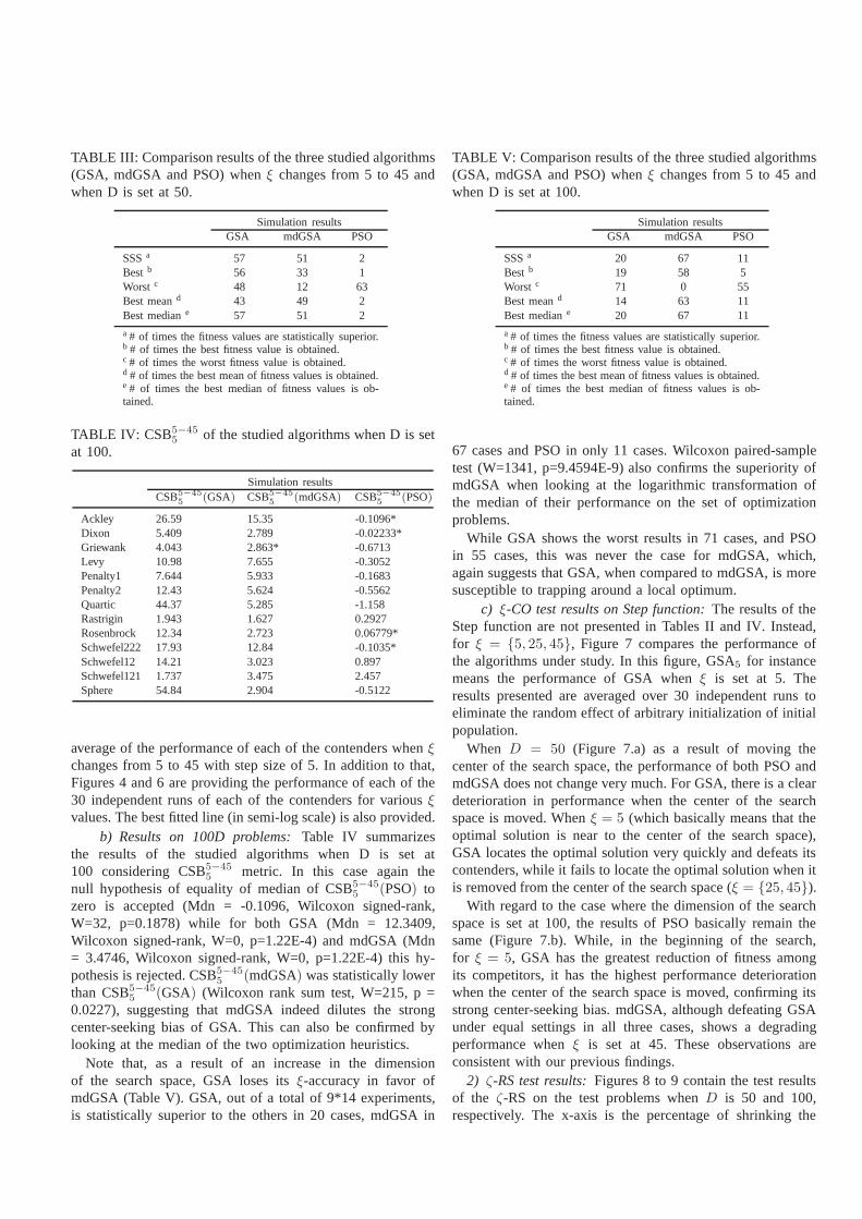
TABLE III: Comparison results of the three studied algorithms(GSA, mdGSA and PSO) whenξ changes from 5 to 45 andwhen D is set at 50.

Simulation resultsGSA mdGSA PSO

SSSa 57 51 2Best b 56 33 1Worst c 48 12 63Best meand 43 49 2Best mediane 57 51 2

a # of times the fitness values are statistically superior.b # of times the best fitness value is obtained.c # of times the worst fitness value is obtained.d # of times the best mean of fitness values is obtained.e # of times the best median of fitness values is ob-tained.

TABLE IV: CSB5−455 of the studied algorithms when D is set

at 100.

Simulation resultsCSB5−45

5(GSA) CSB5−45

5(mdGSA) CSB5−45

5(PSO)

Ackley 26.59 15.35 -0.1096*Dixon 5.409 2.789 -0.02233*Griewank 4.043 2.863* -0.6713Levy 10.98 7.655 -0.3052Penalty1 7.644 5.933 -0.1683Penalty2 12.43 5.624 -0.5562Quartic 44.37 5.285 -1.158Rastrigin 1.943 1.627 0.2927Rosenbrock 12.34 2.723 0.06779*Schwefel222 17.93 12.84 -0.1035*Schwefel12 14.21 3.023 0.897Schwefel121 1.737 3.475 2.457Sphere 54.84 2.904 -0.5122

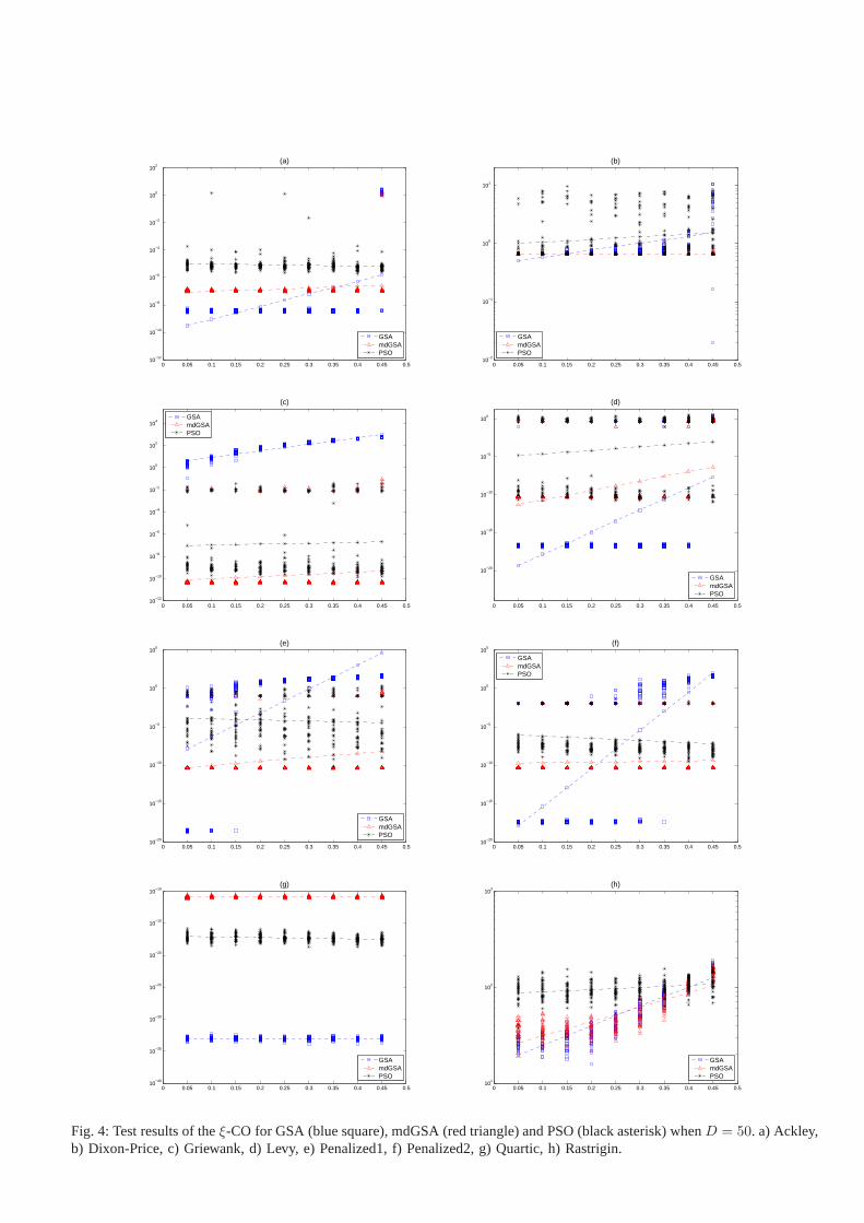
average of the performance of each of the contenders whenξ

changes from 5 to 45 with step size of 5. In addition to that,Figures 4 and 6 are providing the performance of each of the30 independent runs of each of the contenders for variousξ

values. The best fitted line (in semi-log scale) is also provided.b) Results on 100D problems:Table IV summarizes

the results of the studied algorithms when D is set at100 considering CSB5−45

5 metric. In this case again thenull hypothesis of equality of median of CSB5−45

5 (PSO) tozero is accepted (Mdn = -0.1096, Wilcoxon signed-rank,W=32, p=0.1878) while for both GSA (Mdn = 12.3409,Wilcoxon signed-rank, W=0, p=1.22E-4) and mdGSA (Mdn= 3.4746, Wilcoxon signed-rank, W=0, p=1.22E-4) this hy-pothesis is rejected. CSB5−45

5 (mdGSA) was statistically lowerthan CSB5−45

5 (GSA) (Wilcoxon rank sum test, W=215, p =0.0227), suggesting that mdGSA indeed dilutes the strongcenter-seeking bias of GSA. This can also be confirmed bylooking at the median of the two optimization heuristics.

Note that, as a result of an increase in the dimensionof the search space, GSA loses itsξ-accuracy in favor ofmdGSA (Table V). GSA, out of a total of 9*14 experiments,is statistically superior to the others in 20 cases, mdGSA in

TABLE V: Comparison results of the three studied algorithms(GSA, mdGSA and PSO) whenξ changes from 5 to 45 andwhen D is set at 100.




67 cases and PSO in only 11 cases. Wilcoxon paired-sampletest (W=1341, p=9.4594E-9) also confirms the superiority ofmdGSA when looking at the logarithmic transformation ofthe median of their performance on the set of optimizationproblems.

While GSA shows the worst results in 71 cases, and PSOin 55 cases, this was never the case for mdGSA, which,again suggests that GSA, when compared to mdGSA, is moresusceptible to trapping around a local optimum.

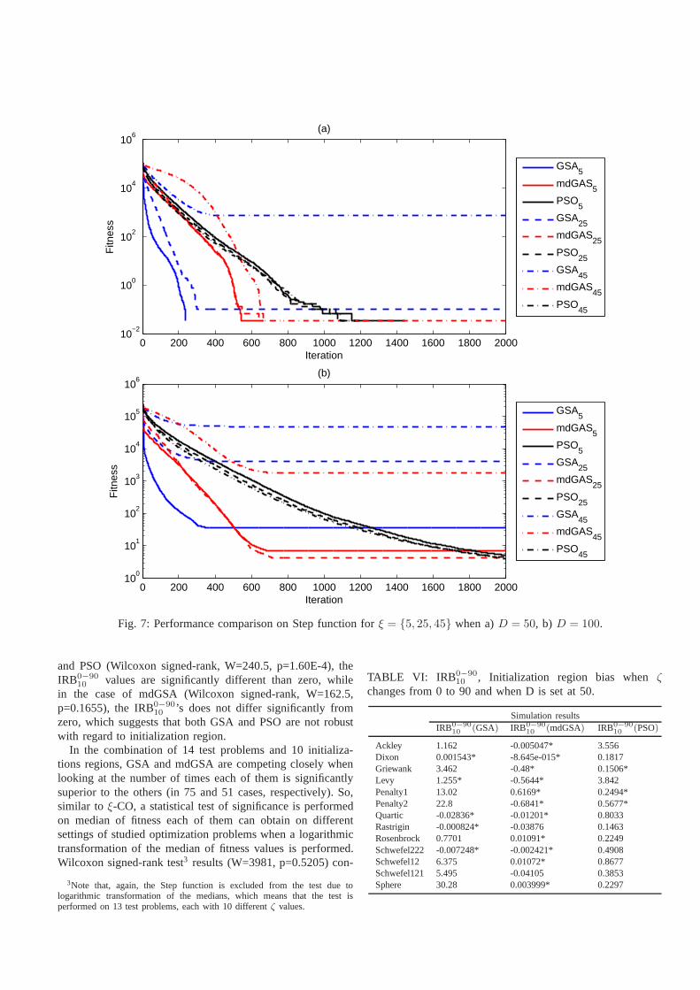
c) ξ-CO test results on Step function:The results of theStep function are not presented in Tables II and IV. Instead,for ξ = {5, 25, 45}, Figure 7 compares the performance ofthe algorithms under study. In this figure, GSA5 for instancemeans the performance of GSA whenξ is set at 5. Theresults presented are averaged over 30 independent runs toeliminate the random effect of arbitrary initialization ofinitialpopulation.

When D = 50 (Figure 7.a) as a result of moving thecenter of the search space, the performance of both PSO andmdGSA does not change very much. For GSA, there is a cleardeterioration in performance when the center of the searchspace is moved. Whenξ = 5 (which basically means that theoptimal solution is near to the center of the search space),GSA locates the optimal solution very quickly and defeats itscontenders, while it fails to locate the optimal solution when itis removed from the center of the search space (ξ = {25, 45}).

With regard to the case where the dimension of the searchspace is set at 100, the results of PSO basically remain thesame (Figure 7.b). While, in the beginning of the search,for ξ = 5, GSA has the greatest reduction of fitness amongits competitors, it has the highest performance deteriorationwhen the center of the search space is moved, confirming itsstrong center-seeking bias. mdGSA, although defeating GSAunder equal settings in all three cases, shows a degradingperformance whenξ is set at 45. These observations areconsistent with our previous findings.

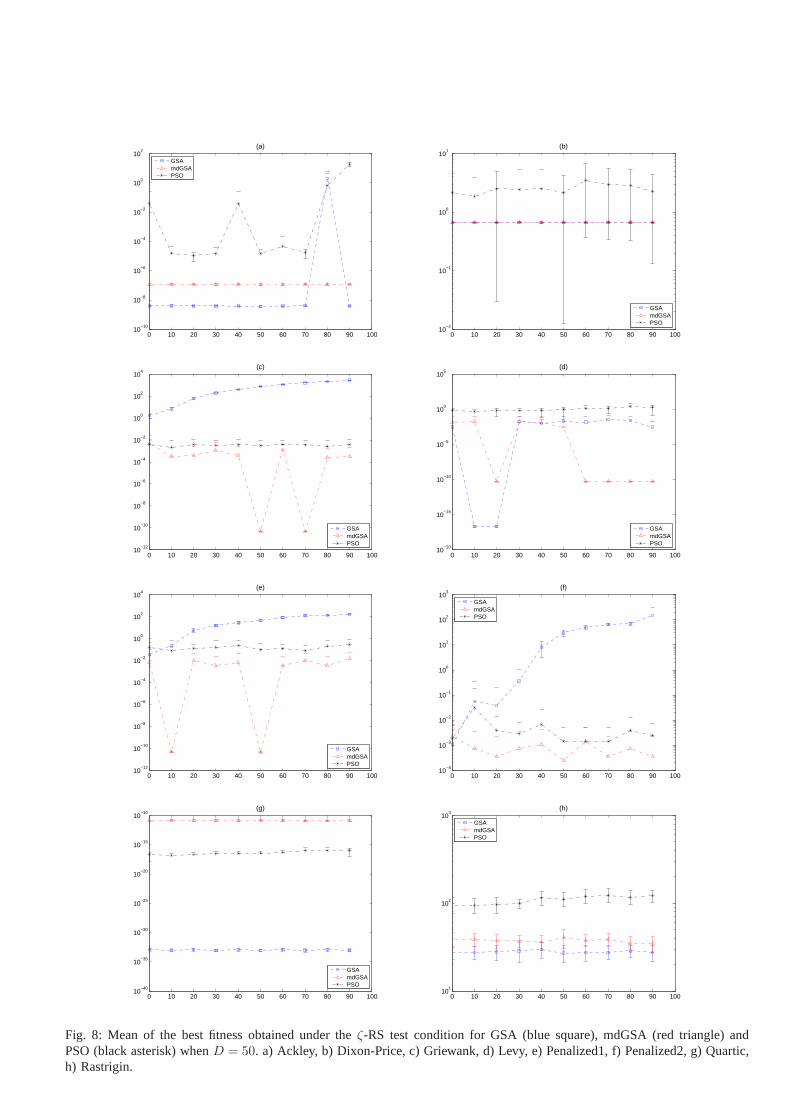
2) ζ-RS test results:Figures 8 to 9 contain the test resultsof the ζ-RS on the test problems whenD is 50 and 100,respectively. The x-axis is the percentage of shrinking the

0 0.05 0.1 0.15 0.2 0.25 0.3 0.35 0.4 0.45 0.510

−12

10−10

10−8

10−6

10−4

10−2

100

102

(a)

GSAmdGSAPSO

0 0.05 0.1 0.15 0.2 0.25 0.3 0.35 0.4 0.45 0.510

−2

10−1

100

101

(b)

GSAmdGSAPSO

0 0.05 0.1 0.15 0.2 0.25 0.3 0.35 0.4 0.45 0.510

−12

10−10

10−8

10−6

10−4

10−2

100

102

104

(c)

GSAmdGSAPSO

0 0.05 0.1 0.15 0.2 0.25 0.3 0.35 0.4 0.45 0.5

10−20

10−15

10−10

10−5

100

(d)

GSAmdGSAPSO

0 0.05 0.1 0.15 0.2 0.25 0.3 0.35 0.4 0.45 0.510

−20

10−15

10−10

10−5

100

105

(e)

GSAmdGSAPSO

0 0.05 0.1 0.15 0.2 0.25 0.3 0.35 0.4 0.45 0.510

−20

10−15

10−10

10−5

100

105

(f)

GSAmdGSAPSO

0 0.05 0.1 0.15 0.2 0.25 0.3 0.35 0.4 0.45 0.510

−40

10−35

10−30

10−25

10−20

10−15

10−10

(g)

GSAmdGSAPSO

0 0.05 0.1 0.15 0.2 0.25 0.3 0.35 0.4 0.45 0.510

1

102

103

(h)

GSAmdGSAPSO

Fig. 4: Test results of theξ-CO for GSA (blue square), mdGSA (red triangle) and PSO (black asterisk) whenD = 50. a) Ackley,b) Dixon-Price, c) Griewank, d) Levy, e) Penalized1, f) Penalized2, g) Quartic, h) Rastrigin.

0 0.05 0.1 0.15 0.2 0.25 0.3 0.35 0.4 0.45 0.510

0

101

102

103

104

(i)

GSAmdGSAPSO

0 0.05 0.1 0.15 0.2 0.25 0.3 0.35 0.4 0.45 0.510

−8

10−7

10−6

10−5

10−4

10−3

10−2

10−1

100

101

(j)

GSAmdGSAPSO

0 0.05 0.1 0.15 0.2 0.25 0.3 0.35 0.4 0.45 0.510

1

102

103

104

105

106

107

108

(k)

GSAmdGSAPSO

0 0.05 0.1 0.15 0.2 0.25 0.3 0.35 0.4 0.45 0.510

−10

10−8

10−6

10−4

10−2

100

102

104

(l)

GSAmdGSAPSO

0 0.05 0.1 0.15 0.2 0.25 0.3 0.35 0.4 0.45 0.510

−18

10−16

10−14

10−12

10−10

10−8

10−6

10−4

10−2

100

102

(m)

GSAmdGSAPSO

0 0.05 0.1 0.15 0.2 0.25 0.3 0.35 0.4 0.45 0.510

0

101

102

103

104

(n)

GSAmdGSAPSO

Fig. 4: (continued) Test results of theξ-CO for GSA (blue square), mdGSA (red triangle) and PSO (black asterisk) whenD = 50. i) Rosenbrock, j) Schwefel P2.22 k) Schwefel P1.2, l) Schwefel P2.21, m) Sphere, n) Step.

initialization region and the y-axis is the performance averagedover 30 independent runs. An algorithm with no IRB has theopportunity to explore areas outside the initialization region.

Throughout this study,ζs is set at 10 whenζL = 0 andζU = 90. A line best fitted to 10*30 observations has a slopeof IRBζL−ζU

ζs.

Tables VI and VIII present an estimation of the degreeof change in the quality of best-of-run of each optimizationheuristic as a result of shrinking the initialization region, whenthe dimension of problems are set at 50 and 100, respectively.

Here, again, in each table asterisks symbols are used todenote no statistically significant association between observedchange in estimation of best-of-run as a result of change inζ

using F-statistics.For the same reason asξ-CO, the Step function is excluded

from the Tables VI and VIII. Instead, for some selectedζ

values, its convergence curse is visualized in Figure 10.To compareζ-accuracy of the optimization heuristics under

study, we look at the number of times one is statisticallysuperior to the others and the number of times one has the

0 5 10 15 20 25 30 35 40 45 5010

−8

10−6

10−4

10−2

100

102

(a)

GSAmdGSAPSO

0 5 10 15 20 25 30 35 40 45 5010

−1

100

101

102

103

104

(b)

GSAmdGSAPSO

0 5 10 15 20 25 30 35 40 45 5010

−3

10−2

10−1

100

101

102

103

104

(c)

GSAmdGSAPSO

0 5 10 15 20 25 30 35 40 45 5010

−3

10−2

10−1

100

101

102

(d)

GSAmdGSAPSO

0 5 10 15 20 25 30 35 40 45 5010

−2

10−1

100

101

102

103

104

105

(e)

GSAmdGSAPSO

0 5 10 15 20 25 30 35 40 45 5010

−2

100

102

104

106

108

(f)

GSAmdGSAPSO

0 5 10 15 20 25 30 35 40 45 5010

−35

10−30

10−25

10−20

10−15

10−10

10−5

100

(g)

GSAmdGSAPSO

0 5 10 15 20 25 30 35 40 45 5010

1

102

103

(h)

GSAmdGSAPSO

Fig. 5: Mean of the best fitness obtained under theξ-CO test condition for GSA (blue square), mdGSA (red triangle) and PSO(black asterisk) whenD = 100. a) Ackley, b) Dixon-Price, c) Griewank, d) Levy, e) Penalized1, f) Penalized2, g) Quartic,h) Rastrigin.

0 5 10 15 20 25 30 35 40 45 5010

1

102

103

104

105

106

107

108

(i)

GSAmdGSAPSO

0 5 10 15 20 25 30 35 40 45 5010

−3

10−2

10−1

100

101

102

103

(j)

GSAmdGSAPSO

0 5 10 15 20 25 30 35 40 45 5010

3

104

105

106

107

108

109

(k)

GSAmdGSAPSO

0 5 10 15 20 25 30 35 40 45 5010

−1

100

101

102

(l)

GSAmdGSAPSO

0 5 10 15 20 25 30 35 40 45 5010

−20

10−15

10−10

10−5

100

105

(m)

GSAmdGSAPSO

0 5 10 15 20 25 30 35 40 45 5010

−1

100

101

102

103

104

105

(n)

GSAmdGSAPSO

Fig. 5: (continued) Mean of the best fitness obtained under the ξ-CO test condition for GSA (blue square), mdGSA (redtriangle) and PSO (black asterisk) whenD = 100. i) Rosenbrock, j) Schwefel P2.22 k) Schwefel P1.2, l) Schwefel P2.21,m) Sphere, n) Step.

0 0.05 0.1 0.15 0.2 0.25 0.3 0.35 0.4 0.45 0.510

−12

10−10

10−8

10−6

10−4

10−2

100

102

(a)

GSAmdGSAPSO

0 0.05 0.1 0.15 0.2 0.25 0.3 0.35 0.4 0.45 0.510

−1

100

101

102

103

104

(b)

GSAmdGSAPSO

0 0.05 0.1 0.15 0.2 0.25 0.3 0.35 0.4 0.45 0.5

10−10

10−8

10−6

10−4

10−2

100

102

104

106

(c)

GSAmdGSAPSO

0 0.05 0.1 0.15 0.2 0.25 0.3 0.35 0.4 0.45 0.5

10−20

10−15

10−10

10−5

100

(d)

GSAmdGSAPSO

0 0.05 0.1 0.15 0.2 0.25 0.3 0.35 0.4 0.45 0.5

10−15

10−10

10−5

100

105

(e)

GSAmdGSAPSO

0 0.05 0.1 0.15 0.2 0.25 0.3 0.35 0.4 0.45 0.510

−12

10−10

10−8

10−6

10−4

10−2

100

102

104

106

108

(f)

GSAmdGSAPSO

0 0.05 0.1 0.15 0.2 0.25 0.3 0.35 0.4 0.45 0.5

10−40

10−35

10−30

10−25

10−20

10−15

10−10

10−5

100

(a)

GSAmdGSAPSO

0 0.05 0.1 0.15 0.2 0.25 0.3 0.35 0.4 0.45 0.510

1

102

103

(h)

GSAmdGSAPSO

Fig. 6: Test results of theξ-CO for for GSA (blue square), mdGSA (red triangle) and PSO (black asterisk) whenD = 100.a) Ackley, b) Dixon-Price, c) Griewank, d) Levy, e) Penalized1, f) Penalized2, g) Quartic, h) Rastrigin.

0 0.05 0.1 0.15 0.2 0.25 0.3 0.35 0.4 0.45 0.510

1

102

103

104

105

106

107

108

(i)

GSAmdGSAPSO

0 0.05 0.1 0.15 0.2 0.25 0.3 0.35 0.4 0.45 0.510

−7

10−6

10−5

10−4

10−3

10−2

10−1

100

101

102

103

(j)

GSAmdGSAPSO

0 0.05 0.1 0.15 0.2 0.25 0.3 0.35 0.4 0.45 0.510

3

104

105

106

107

108

109

(k)

GSAmdGSAPSO

0 0.05 0.1 0.15 0.2 0.25 0.3 0.35 0.4 0.45 0.510

−6

10−5

10−4

10−3

10−2

10−1

100

101

102

(l)

GSAmdGSAPSO

0 0.05 0.1 0.15 0.2 0.25 0.3 0.35 0.4 0.45 0.510

−20

10−15

10−10

10−5

100

105

1010

(m)

GSAmdGSAPSO

0 0.05 0.1 0.15 0.2 0.25 0.3 0.35 0.4 0.45 0.510

0

101

102

103

104

105

106

(n)

GSAmdGSAPSO

Fig. 6: (continued) Test results of theξ-CO for GSA (blue square), mdGSA (red triangle) and PSO (black asterisk) whenD = 100. i) Rosenbrock, j) Schwefel P2.22 k) Schwefel P1.2, l) Schwefel P2.21, m) Sphere, n) Step.

worst fitness (Tables VII and IX). For each optimizationheuristic, the number of test problems equals 10*14 (10ζ

values for each of the 14 problems). We also report the numberof times an optimization method has the best performance,best mean and best median when it is statistically superior.The number of times each has the worst fitness is reported aswell.

a) Results on 50D problems:In 10 of the 13 optimizationproblems, the performance of the PSO algorithm degradesas a result of shrinking the initialization space. However

compared to GSA, its IRB0−9010 is small. The performance of

the GSA on eight optimization problem degrades underζ-RStest. The mdGSA is more robust to the initialization regionand is nearly a straight line in 11 of the 13 experiments. Theslope is significantly different than zero in only two cases.In both of these cases, the slope is negative, meaning that theperformance of the algorithm increases as a result of shrinkingthe initialization region. A possible explanation for thiswillbe suggested later.

For GSA (Wilcoxon signed-rank, W=227.5, p=0.0012)

0 200 400 600 800 1000 1200 1400 1600 1800 200010

−2

100

102

104

106

Iteration

Fitn

ess

(a)

GSA5

mdGAS5

PSO5

GSA25

mdGAS25

PSO25

GSA45

mdGAS45

PSO45

0 200 400 600 800 1000 1200 1400 1600 1800 200010

0

101

102

103

104

105

106

Iteration

Fitn

ess

(b)

GSA5

mdGAS5

PSO5

GSA25

mdGAS25

PSO25

GSA45

mdGAS45

PSO45

Fig. 7: Performance comparison on Step function forξ = {5, 25, 45} when a)D = 50, b) D = 100.

and PSO (Wilcoxon signed-rank, W=240.5, p=1.60E-4), theIRB0−90

10 values are significantly different than zero, whilein the case of mdGSA (Wilcoxon signed-rank, W=162.5,p=0.1655), the IRB0−90

10 ’s does not differ significantly fromzero, which suggests that both GSA and PSO are not robustwith regard to initialization region.

In the combination of 14 test problems and 10 initializa-tions regions, GSA and mdGSA are competing closely whenlooking at the number of times each of them is significantlysuperior to the others (in 75 and 51 cases, respectively). So,similar to ξ-CO, a statistical test of significance is performedon median of fitness each of them can obtain on differentsettings of studied optimization problems when a logarithmictransformation of the median of fitness values is performed.Wilcoxon signed-rank test3 results (W=3981, p=0.5205) con-

3Note that, again, the Step function is excluded from the testdue tologarithmic transformation of the medians, which means that the test isperformed on 13 test problems, each with 10 differentζ values.

TABLE VI: IRB 0−90

10 , Initialization region bias whenζchanges from 0 to 90 and when D is set at 50.

Simulation resultsIRB0−90

10(GSA) IRB0−90

10(mdGSA) IRB0−90

10(PSO)

Ackley 1.162 -0.005047* 3.556Dixon 0.001543* -8.645e-015* 0.1817Griewank 3.462 -0.48* 0.1506*Levy 1.255* -0.5644* 3.842Penalty1 13.02 0.6169* 0.2494*Penalty2 22.8 -0.6841* 0.5677*Quartic -0.02836* -0.01201* 0.8033Rastrigin -0.000824* -0.03876 0.1463Rosenbrock 0.7701 0.01091* 0.2249Schwefel222 -0.007248* -0.002421* 0.4908Schwefel12 6.375 0.01072* 0.8677Schwefel121 5.495 -0.04105 0.3853Sphere 30.28 0.003999* 0.2297

TABLE VII: Comparison results of the three studied algo-rithms (GSA, mdGSA and PSO) whenζ changes from 0 to90 and when D is set at 50.




firm that there is no significant difference between the perfor-mance of GSA and mdGSA. So, mdGSA and GSA come injoint first place, while PSO comes in second place.

In 69 cases, PSO has the worst fitness over 30 runs, whileGSA, with 58 cases, comes in second place and mdGSA,with 11 cases, shows the best performance. This suggests thatmdGSA is less susceptible to the attraction of local optima.Table VII summarizes the results.

b) Results on 100D problems:In Table VIII, the slopeof the line fitted to observed best-of-run fitness values foreach benchmark problem is presented when D is set at 100.IRB0−90

10 (PSO) has significantly positive associations withζin all cases. GSA has a significantly positive IRB0−90

10 in11 of the total of 13 cases, while IRB0−90

10 (mdGSA) hasno significant positive associations withζ. This suggeststhat GSA (Wilcoxon signed-rank, W=247, p=9.97E-5) andPSO (Wilcoxon signed-rank, W=260, p=4.15E-6) both havesignificant initialization region bias when D is set at 100,while mdGSA (Wilcoxon signed-rank, W=156, p=.29) hasIRB values that are significantly close to zero.

As was the case when the dimension of the test problemsis set at 50, mdGSA again has some negative IRB values. Anintuitive explanation for this observation goes as follows. Dueto high mass discrimination of mdGSA, when the initializationregion is small compared to the entire design space, the particlewith the highest fitness that is equivalent to highest mass isbetter able to direct the entire swarm towards the optimalsolution. As a result the algorithm performs slightly bettercompared to when the initialization is taken in the entire searchspace. It is important to point out that the improvement isnot visible in most of the cases from Figures 8 and 9 andthat this improvements, in all 13 cases, has no significantcorrelation withζ, confirmed by analysis of covariance (F-test). When compared to GSA, mdGSA has significantly lessIRB (Wilcoxon rank sum test, W=246, p = 1.65E-4). So,in terms of robustness in change in IR, mdGSA defeats itscompetitors.

Summarized in Table IX, mdGSA presents higherζ-accuracy compared to its two competitors. With 87 cases of

TABLE VIII: IRB 0−90

10 , Initialization region bias whenζchanges from 0 to 90 and when D is set at 100.

Simulation resultsIRB0−90

10(GSA) IRB0−90

10(mdGSA) IRB0−90

10(PSO)

Ackley 11.29 0.05864* 1.153Dixon 0.286 -0.02044* 0.1956Griewank 2.623 0.4001* 0.2914Levy 2.865 -0.05098* 0.9592Penalty1 10.06 0.03984* 0.3084Penalty2 10.05 0.007134* 0.1713Quartic -0.04523* -0.002844* 0.9314Rastrigin 0.00851* -0.02011* 0.2116Rosenbrock 8.438 -0.0005933* 0.4377Schwefel222 2.635 -0.2029* 0.6911Schwefel12 7.004 -0.01445* 1.124Schwefel121 1.116 -0.09892* 0.3697Sphere 21.57 0.004679* 0.2886

TABLE IX: Comparison results of the three studied algorithms(GSA, mdGSA and PSO) whenζ changes from 0 to 90 andwhen D is set at 100.




significant superiority out of total of 14*10 cases, mdGSAranked in the first place, followed by GSA, with 26 cases, andPSO, with zero cases. Wilcoxon paired-sample test (W=1735,p=4.5869E-9) also confirms the superiority of mdGSA whenlooking at the logarithmic transformation of the median oftheir performance.

GSA has the worst fitness in 75 cases, and PSO in 65 cases.mdGSA has the smallest number of worst fitness comparedto that of GSA and PSO, confirming its superiority over itscompetitors in terms ofζ-accuracy. This again suggests thatmdGSA is less susceptible to premature convergence to localoptimum when compared to PSO and GSA.

c) ζ-RS test results on Step function:Again for theStep function, the results are not presented in Tables VIand VIII. So the performance of the studied algorithms whenζ = {10, 50, 90} are presented in Figure 10.

When D = 50 (Figure 10.a) GSA10 has a sharp fitnessdecrease. The performance degrades significantly as a resultof shrinking the initialization region (GSA50 and GSA90).For mdGSA, the performance slightly changes as a result ofchange in IR, but the pattern was not clear. The performanceof PSO was basically the same under different IRs.

0 10 20 30 40 50 60 70 80 90 10010

−10

10−8

10−6

10−4

10−2

100

102

(a)

GSAmdGSAPSO

0 10 20 30 40 50 60 70 80 90 10010

−2

10−1

100

101

(b)

GSAmdGSAPSO

0 10 20 30 40 50 60 70 80 90 10010

−12

10−10

10−8

10−6

10−4

10−2

100

102

104

(c)

GSAmdGSAPSO

0 10 20 30 40 50 60 70 80 90 10010

−20

10−15

10−10

10−5

100

105

(d)

GSAmdGSAPSO

0 10 20 30 40 50 60 70 80 90 10010

−12

10−10

10−8

10−6

10−4

10−2

100

102

104

(e)

GSAmdGSAPSO

0 10 20 30 40 50 60 70 80 90 10010

−4

10−3

10−2

10−1

100

101

102

103

(f)

GSAmdGSAPSO

0 10 20 30 40 50 60 70 80 90 10010

−40

10−35

10−30

10−25

10−20

10−15

10−10

(g)

GSAmdGSAPSO

0 10 20 30 40 50 60 70 80 90 10010

1

102

103

(h)

GSAmdGSAPSO

Fig. 8: Mean of the best fitness obtained under theζ-RS test condition for GSA (blue square), mdGSA (red triangle) andPSO (black asterisk) whenD = 50. a) Ackley, b) Dixon-Price, c) Griewank, d) Levy, e) Penalized1, f) Penalized2, g) Quartic,h) Rastrigin.

0 10 20 30 40 50 60 70 80 90 100

101

102

103

104

105

(i)

GSAmdGSAPSO

0 10 20 30 40 50 60 70 80 90 10010

−8

10−7

10−6

10−5

(j)

GSAmdGSAPSO

0 10 20 30 40 50 60 70 80 90 10010

2

103

104

105

106

107

108

(k)

GSAmdGSAPSO

0 10 20 30 40 50 60 70 80 90 10010

−10

10−8

10−6

10−4

10−2

100

102

(l)

GSAmdGSAPSO

0 10 20 30 40 50 60 70 80 90 10010

−20

10−15

10−10

10−5

100

105

(m)

GSAmdGSAPSO

0 10 20 30 40 50 60 70 80 90 10010

−2

10−1

100

101

102

103

104

105

(n)

GSAmdGSAPSO

Fig. 8: (continued) Mean of the best fitness obtained under the ζ-RS test condition for GSA (blue), mdGSA (red) and PSO(black) whenD = 50. a) Dixon-Price, b) Quartic, c) Schwefel P1.2, d) Schwefel P2.21, e) Sphere, f) Step.

GSA10, when the dimension is set at 100 (Figure 10.b),has a sharp fitness change and becomes almost stagnantafter approximately 300 iterations on average. As a resultof shrinking the search space, there is a clear pattern indeterioration of the performance GSA. PSO exhibits similarpatterns as expected, shrinking the initialization regiondoesnot appear to affect its performance. For mdGSA, on the Stepfunction and when the dimension of the problem is set at100, moving the optimum away from the center of the searchspace improves the performance slightly. These observations

are compatible with our former findings.

B. Experiment 2: Gene regulatory network model identifica-tion

Gene regulatory network (GRN) model identification canbe a good real-world application to test the center-seekingbe-havior and convergence speed of the optimization algorithms,since the optimal solution is, naturally, not at the center ofthe search space. Moreover the problem is highly nonlinearand complex [21], [29], [56]. A short introduction to GRN is

0 10 20 30 40 50 60 70 80 90 10010

−10

10−8

10−6

10−4

10−2

100

102

(a)

GSAmdGSAPSO

0 10 20 30 40 50 60 70 80 90 10010

−1

100

101

102

(b)

GSAmdGSAPSO

0 10 20 30 40 50 60 70 80 90 10010

−2

10−1

100

101

102

103

104

(c)

GSAmdGSAPSO

0 10 20 30 40 50 60 70 80 90 10010

−3

10−2

10−1

100

101

102

103

(d)

GSAmdGSAPSO

0 10 20 30 40 50 60 70 80 90 10010

−2

100

102

104

106

108

1010

(e)

GSAmdGSAPSO

0 10 20 30 40 50 60 70 80 90 10010

−2

100

102

104

106

108

1010

(f)

GSAmdGSAPSO

0 10 20 30 40 50 60 70 80 90 10010

−40

10−30

10−20

10−10

100

(g)

GSAmdGSAPSO

0 10 20 30 40 50 60 70 80 90 10010

1

102

103

(h)

GSAmdGSAPSO

Fig. 9: Mean of the best fitness obtained under theζ-RS test condition for GSA (blue square), mdGSA (red triangle) and PSO(black asterisk) whenD = 100. a) Ackley, b) Dixon-Price, c) Griewank, d) Levy, e) Penalized1, f) Penalized2, g) Quartic,h) Rastrigin.

0 10 20 30 40 50 60 70 80 90 10010

0

102

104

106

108

1010

(i)

GSAmdGSAPSO

0 10 20 30 40 50 60 70 80 90 10010

−5

10−4

10−3

10−2

10−1

100

101

(j)

GSAmdGSAPSO

0 10 20 30 40 50 60 70 80 90 10010

3

104

105

106

107

108

109

1010

(k)

GSAmdGSAPSO

0 10 20 30 40 50 60 70 80 90 10010

−1

100

101

102

(l)

GSAmdGSAPSO

0 10 20 30 40 50 60 70 80 90 10010

−20

10−15

10−10

10−5

100

105

1010

(m)

GSAmdGSAPSO

0 10 20 30 40 50 60 70 80 90 10010

−2

10−1

100

101

102

103

104

105

106

(n)

GSAmdGSAPSO

Fig. 9: (continued) Mean of the best fitness obtained under the ζ-RS test condition for GSA (blue square), mdGSA (redtriangle) and PSO (black asterisk) whenD = 100. i) Rosenbrock, j) Schwefel P2.22 k) Schwefel P1.2, l) Schwefel P2.21,m) Sphere, n) Step.

0 200 400 600 800 1000 1200 1400 1600 1800 200010

−2

100

102

104

106

Iteration

Fitn

ess

(a)

GSA10

mdGAS10

PSO10

GSA50

mdGAS50

PSO50

GSA90

mdGAS90

PSO90

0 200 400 600 800 1000 1200 1400 1600 1800 200010

0

101

102

103

104

105

106

Iteration

Fitn

ess

(b)

GSA10

mdGAS10

PSO10

GSA50

mdGAS50

PSO50

GSA90

mdGAS90

PSO90

Fig. 10: Performance comparison on Step function forζ = {10, 50, 100} when a)D = 50, b) D = 100.

provided below.1) Gene regulatory Network:The activation and inhibition

of genes are governed by factors within a cellular environmentand outside of the cell. This level of activation and inhibitionof genes is integrated by gene regulatory networks (GRNs),forming an organizational level in the cell with complexdynamics [9].

GRNs in a cell are complex dynamic network of interactionsbetween the products of genes (mRNAs) and the proteins theyproduce, some of which in return act as regulators of theexpression of other genes (or even their own gene) in theproduction of mRNA. While low cost methods to monitorgene expression through microarrays exist, we still know littleabout the complex interactions of these cellular components.Mathematical modeling of GRNs is becoming popular in thepost-genome era [30], [31]. It provides a powerful tool, notonly for a better understanding of such complex systems, butalso for developing new hypotheses on underlying mechanisms

of gene regulation. The availability of high-throughput tech-nologies provides time course expression data, and a GRNmodel built by reverse engineering, may explain the data [39].Since many diseases are the result of polygenic and pleiotropiceffects controlled by multiple genes, genome-wide interactionanalysis is preferable to single-locus studies. Readers lookingfor more information on GRN might refer to Schlitt [53].

2) S-system gene network model:Usually, sets of ordinarydifferential equations (ODEs) are used as mathematical modelsfor these systems [59]. S-system approaches, on the otherhand, use time-independent variables to model these processes.Assuming the concentration ofN proteins, mRNAs, or smallmolecules at timet is given by yt1, y

t2, . . . , y

ti , . . . , y

tN , S-

systems model the temporal evolution of theith component attime t by power-law functions of the form (17).

TABLE X: S-System Parameters adopted for model valida-tion [58].

Network parametersi αi βi gi1 gi2 hi1 gi2

1 3 3 0 2.5 -1 02 3 3 -2.5 0 0 2

dytidt

= αi

N∏

j=1

(ytj)gij

− βi

N∏

j=1

(ytj)hij

. (17)

The first term represents all factors that promote the ex-pression of componenti at time t, yti , whereas the secondterm represents all factors that inhibit its expression. Inabiochemical engineering context, the non-negative parametersαi , βi are called rate constants, and real-valued exponentsgij (G matrix, [G]) andhij (H matrix, [H ]) are referred to askinetic order for synthesis and kinetic order for degradation,respectively.{α, β, [G], [H ]} are the parameters that define the S-system.

The total number of parameters in the S-system is2N(N+1).The parameter estimation is used to determine model param-eters so that the dynamic profiles fit the observation.

3) Population based S-system model parameter identifi-cation: S-system based GRN inference was formulated byTominaga et al. [58] as an optimization problem to minimizethe difference between the model and the system. To guide thepopulation in the search space, some measure of discriminationis needed. The most commonly used quality assessment cri-terion is the relative mean quadratic discrepancy between theobserved expression patternyti and the model outputyti [40].

f =

N∑

i=1

T∑

t=1

(

yti − ytiyti

)2

, (18)

whereT represents the number of time points.To assess the performance of the methodologies studied

here, a gene regulatory network consist of two genes generatedby the parameters provided in Table X is adopted [58]. Inthe original implementation, the search space forαi and βi

is limited to [0.0, 20] and for gij and hij to [−4.0, 4.0]and y01 and y02 are set at0.7 and 0.3, respectively. The geneexpression levels are plotted in Figure 11 and each consist of50 time course of expression level per gene. To study the effectof initialization region on the converge of the optimizationalgorithms the initialization set to cover part of the searchspace. In this study,αi and βi is initialized in [10, 20] andboth gij andhij to [2.0, 4.0].

4) Results:The fitness transitions of studied methodologiesare plotted in Figure 12. All algorithms discussed here startwith a randomly generated population of solutions, whichmeans they all start with close fitness values. The Figures areaveraged over 30 independent runs.

0 0.5 1 1.5 20

0.2

0.4

0.6

0.8

1

1.2

1.4

1.6

1.8

2

Con

cent

ratio

n

Time

Gene 1Gene 2

Fig. 11: Target time dynamics of adopted gene network.

0 500 1000 1500 2000 2500 3000 3500 4000

2

4

6

8

10

12

14

Number of iteration

Fitn

ess

GSAmdGSAPSO

Fig. 12: Performance comparison of the GSA, mdGSA andPSO on GRN parameter identification.

All three OAs start with a sharp fitness decrease in thebeginning. GSA almost stagnates after approximately 2,000iterations. mdGSA shows a much better progression comparedto PSO and GSA.

As shown in Table XI, the results of the proposed mdGSAare better than those of GSA when the standard cut-off forconsidering ap-value for a statistically significant differenceis set atp < 0.05. While mdGSA is not significantly superiorto PSO, it shows a better performance, with a smaller standarddeviation.

VI. D ISCUSSIONS

The heuristics we studied are compared on the basis oftheir robustness and accuracy (performance). We divided theevaluation of robustness into the following two assessments:

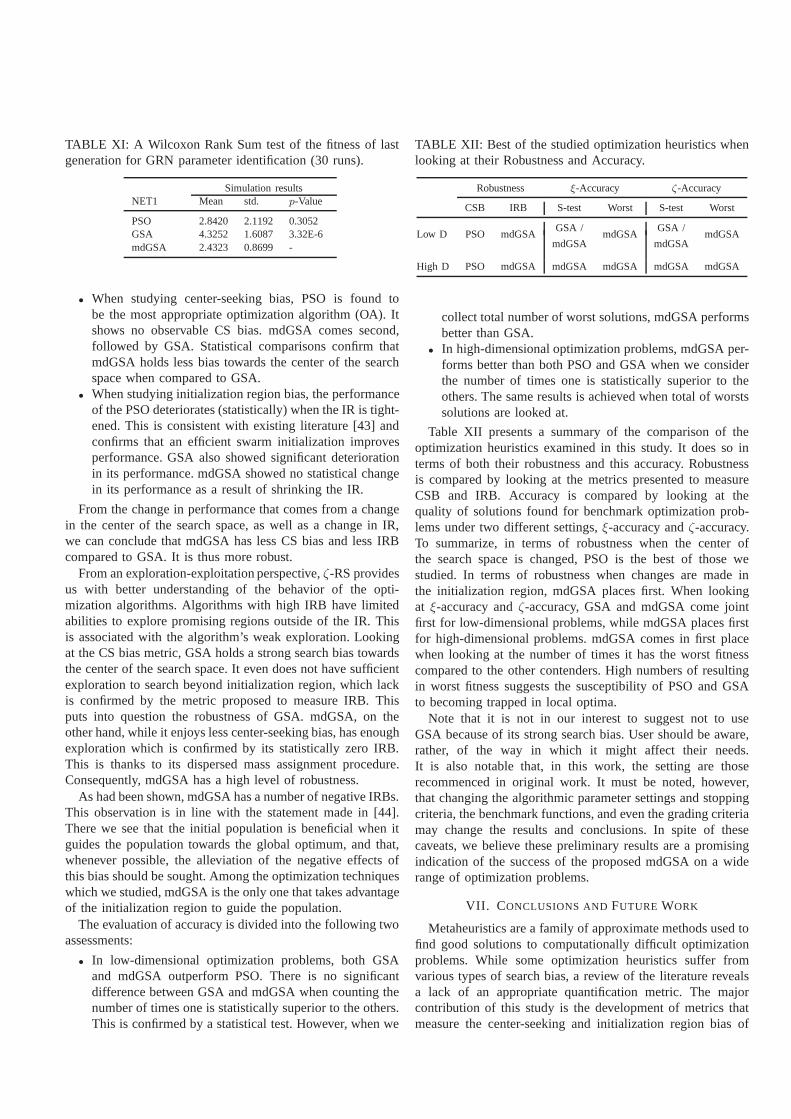
TABLE XI: A Wilcoxon Rank Sum test of the fitness of lastgeneration for GRN parameter identification (30 runs).

Simulation resultsNET1 Mean std. p-Value

PSO 2.8420 2.1192 0.3052GSA 4.3252 1.6087 3.32E-6mdGSA 2.4323 0.8699 -

• When studying center-seeking bias, PSO is found tobe the most appropriate optimization algorithm (OA). Itshows no observable CS bias. mdGSA comes second,followed by GSA. Statistical comparisons confirm thatmdGSA holds less bias towards the center of the searchspace when compared to GSA.

• When studying initialization region bias, the performanceof the PSO deteriorates (statistically) when the IR is tight-ened. This is consistent with existing literature [43] andconfirms that an efficient swarm initialization improvesperformance. GSA also showed significant deteriorationin its performance. mdGSA showed no statistical changein its performance as a result of shrinking the IR.

From the change in performance that comes from a changein the center of the search space, as well as a change in IR,we can conclude that mdGSA has less CS bias and less IRBcompared to GSA. It is thus more robust.

From an exploration-exploitation perspective,ζ-RS providesus with better understanding of the behavior of the opti-mization algorithms. Algorithms with high IRB have limitedabilities to explore promising regions outside of the IR. Thisis associated with the algorithm’s weak exploration. Lookingat the CS bias metric, GSA holds a strong search bias towardsthe center of the search space. It even does not have sufficientexploration to search beyond initialization region, whichlackis confirmed by the metric proposed to measure IRB. Thisputs into question the robustness of GSA. mdGSA, on theother hand, while it enjoys less center-seeking bias, has enoughexploration which is confirmed by its statistically zero IRB.This is thanks to its dispersed mass assignment procedure.Consequently, mdGSA has a high level of robustness.

As had been shown, mdGSA has a number of negative IRBs.This observation is in line with the statement made in [44].There we see that the initial population is beneficial when itguides the population towards the global optimum, and that,whenever possible, the alleviation of the negative effectsofthis bias should be sought. Among the optimization techniqueswhich we studied, mdGSA is the only one that takes advantageof the initialization region to guide the population.

The evaluation of accuracy is divided into the following twoassessments:

• In low-dimensional optimization problems, both GSAand mdGSA outperform PSO. There is no significantdifference between GSA and mdGSA when counting thenumber of times one is statistically superior to the others.This is confirmed by a statistical test. However, when we

TABLE XII: Best of the studied optimization heuristics whenlooking at their Robustness and Accuracy.

Robustness ξ-Accuracy ζ-Accuracy

CSB IRB S-test Worst S-test Worst

GSA / GSA /Low D PSO mdGSA

mdGSAmdGSA

mdGSAmdGSA

High D PSO mdGSA mdGSA mdGSA mdGSA mdGSA

collect total number of worst solutions, mdGSA performsbetter than GSA.

• In high-dimensional optimization problems, mdGSA per-forms better than both PSO and GSA when we considerthe number of times one is statistically superior to theothers. The same results is achieved when total of worstssolutions are looked at.

Table XII presents a summary of the comparison of theoptimization heuristics examined in this study. It does so interms of both their robustness and this accuracy. Robustnessis compared by looking at the metrics presented to measureCSB and IRB. Accuracy is compared by looking at thequality of solutions found for benchmark optimization prob-lems under two different settings,ξ-accuracy andζ-accuracy.To summarize, in terms of robustness when the center ofthe search space is changed, PSO is the best of those westudied. In terms of robustness when changes are made inthe initialization region, mdGSA places first. When lookingat ξ-accuracy andζ-accuracy, GSA and mdGSA come jointfirst for low-dimensional problems, while mdGSA places firstfor high-dimensional problems. mdGSA comes in first placewhen looking at the number of times it has the worst fitnesscompared to the other contenders. High numbers of resultingin worst fitness suggests the susceptibility of PSO and GSAto becoming trapped in local optima.

Note that it is not in our interest to suggest not to useGSA because of its strong search bias. User should be aware,rather, of the way in which it might affect their needs.It is also notable that, in this work, the setting are thoserecommenced in original work. It must be noted, however,that changing the algorithmic parameter settings and stoppingcriteria, the benchmark functions, and even the grading criteriamay change the results and conclusions. In spite of thesecaveats, we believe these preliminary results are a promisingindication of the success of the proposed mdGSA on a widerange of optimization problems.

VII. C ONCLUSIONS ANDFUTURE WORK

Metaheuristics are a family of approximate methods used tofind good solutions to computationally difficult optimizationproblems. While some optimization heuristics suffer fromvarious types of search bias, a review of the literature revealsa lack of an appropriate quantification metric. The majorcontribution of this study is the development of metrics thatmeasure the center-seeking and initialization region biasof

optimization heuristics. We also propose an alternative forcenter offset, as we identified its assumption does not alwayshold.

Using the proposed metrics, the center-seeking (CS) biasand initialization region bias (IRB) of GSA are exposed. Ourinterest in this study was not to improve the performanceof GSA, which can be archived by the integration of usefulheuristics. Rather, it was about presenting a solution to diluteits CS behavior and its IRB. Inspired by our recently intro-duced global optimization process, we established a “mass-dispersed” version of GSA called mdGSA. PSO served as ourbenchmark because it shows no bias towards the center of thesearch space [27].

To further substantiate the limitations and capabilities ofGSA and mdGSA in dealing with real-world optimizationproblems, we want to apply them to a wider range of problems,such as structural design optimization [11], [16], the detectionof hidden information in a spread-spectrum watermarked sig-nal [10], and problems of traffic control [13].

Several optimization heuristics have evolved in the lastdecade to facilitate solving optimization problems (see forexample [22], [38], [49]), some of which suffer from differ-ent types of search bias [61]. The framework presented inthis study appears to be a viable approach when it comesto comparing different optimization heuristics. As part ofour future work, we are interested in using the frameworkproposed here to contrast different optimization heuristicssuitable to handling high-dimensional and complex real-worldoptimization problems.

REFERENCES

[1] P.J. Angeline. Using selection to improve particle swarm optimization.In International Conference on Evolutionary Computation, pages 84–89,1998.

[2] J. Branke. Evolutionary approaches to dynamic optimization problems-updated survey. InGECCO Workshop on evolutionary algorithms fordynamic optimization problems, pages 27–30, 2001.

[3] D. Bratton and J. Kennedy. Defining a standard for particle swarmoptimization. InSwarm Intelligence Symposium, pages 120–127, 2007.

[4] A. Chatterjee, G.K. Mahanti, and N.N. Pathak. Comparative perfor-mance of gravitational search algorithm and modified particle swarmoptimization algorithm for synthesis of thinned scanned concentric ringarray antenna.Progress In Electromagnetics Research B, 25:331–348,2010.

[5] R. Chiong, T. Weise, and Z. Michalewicz.Variants of evolutionaryalgorithms for real-world applications. Springer-Verlag New York Inc,2011.

[6] M. Clerc and J. Kennedy. The particle swarm-explosion, stability, andconvergence in a multidimensional complex space.IEEE Transactionson Evolutionary Computation, 6(1):58–73, 2002.

[7] C. A. Coello Coello. Theoretical and numerical constraint handlingtechniques used with evolutionary algorithms: A survey of the state ofthe art. Computer Methods in Applied Mechanics and Engineering,191(11-12):1245–1287, January 2002.

[8] J. Cohen, P. Cohen, S.G. West, and L.S. Aiken.Applied multipleregression/correlation analysis for the behavioral sciences. LawrenceErlbaum Associates, 2003.

[9] A. Crombach and P. Hogeweg. Evolution of evolvability ingeneregulatory networks.PLoS computational biology, 4(7):e1000112, 2008.

[10] M. Davarynejad, C.W. Ahn, J.L.M. Vrancken, J. van den Berg, andC.A. Coello Coello. Evolutionary hidden information detection bygranulation-based fitness approximation.Applied Soft Computing,10(3):719–729, 2010.

[11] M. Davarynejad, M.R. Akbarzadeh-T, N. Pariz, and A.R. Khorsand.Adaptive fuzzy fitness granulation in structural optimization problems.In 22nd IEEE International Symposium on Intelligent Control (ISIC),pages 172–177, 2007.

[12] M. Davarynejad, Z. Forghany, and J. van den Berg. Mass-dispersed grav-itational search algorithm for gene regulatory network model parameteridentification. InSimulated Evolution and Learning, pages 62–72. 2012.

[13] M. Davarynejad, A. Hegyi, J. Vrancken, and J. van den Berg. Motorwayramp-metering control with queuing consideration usingQ-learning.In 14th International IEEE Conference on Intelligent TransportationSystems (ITSC), pages 1652–1658, 2011.

[14] M. Davarynejad, J. Rezaei, J. Vrancken, J. van den Berg,andC.A. Coello Coello. Accelerating convergence towards the optimalpareto front. InIEEE Congress on Evolutionary Computation (CEC’11),pages 2107–2114, 2011.

[15] M. Davarynejad and J. van den Berg. Simulated big bounce: Acontinuous space global optimizer. Technical report, Faculty of tech-nology policy and management, Delft University of Technology, TheNetherlands, 2012.

[16] M. Davarynejad, J. Vrancken, J. van den Berg, and C.A. Coello Coello.A Fitness Granulation Approach for Large-Scale StructuralDesignOptimization. In Raymond Chiong, Thomas Weise, and ZbigniewMichalewicz, editors,Variants of Evolutionary Algorithms for Real-World Applications, pages 245–280. Springer-Verlag, Berlin, 2012.

[17] R.C. David, R.E. Precup, E.M. Petriu, M.B. Radac, and S. Preitl. Grav-itational search algorithm-based design of fuzzy control systems with areduced parametric sensitivity.Information Sciences, 247(20):154173,2013.

[18] K. Deb, A. Anand, and D. Joshi. A computationally efficient evolution-ary algorithm for real-parameter optimization.Evolutionary computa-tion, 10(4):371–395, 2002.

[19] M. Dorigo and G. Di Caro. Ant colony optimization: a new meta-heuristic. In IEEE Congress on Evolutionary Computation (CEC’99),pages 1470–1477.

[20] S. Duman, U. Guvenc, and N. Yorukeren. Gravitational search algorithmfor economic dispatch with valve-point effects.International Review ofElectrical Engineering (IREE), 5(6), 2010.

[21] Z. Forghany, M. Davarynejad, and B.E. Snaar-Jagalska.Gene regulatorynetwork model identification using artificial bee colony andswarm intel-ligence. InIEEE Conference on Evolutionary Computation (CEC’12),pages 949–954, 2012.

[22] S. Ghosh, S. Das, D. Kundu, K. Suresh, and A. Abraham. Inter-particlecommunication and search-dynamics oflbestparticle swarm optimizers:An analysis.Information Sciences, 182(1):156–168, 2012.

[23] F. Glover and G.A. Kochenberger. Handbook of metaheuristics.Springer, 2003.

[24] U. Guvenc, Y. Sonmez, S. Duman, and N. Yorukeren. Combinedeconomic and emission dispatch solution using gravitational searchalgorithm. Scientia Iranica, 19(6):1754–1762, 2012.

[25] J.H. Holland. Adaptation in natural and artificial systems. Universityof Michigan Press, Ann Arbor, MI, 1975.

[26] D. Karaboga and B. Basturk. A powerful and efficient algorithm fornumerical function optimization: artificial bee colony (abc) algorithm.Journal of Global Optimization, 39(3):459–471, 2007.

[27] J. Kennedy. Some issues and practices for particle swarms. In IEEESwarm Intelligence Symposium (SIS’07), pages 162–169, 2007.

[28] J. Kennedy and R. Eberhart. Particle swarm optimization. In IEEEInternational Conference on Neural Networks, volume 4, pages 1942–1948, 1995.

[29] S. Kikuchi, D. Tominaga, M. Arita, K. Takahashi, and M. Tomita.Dynamic modeling of genetic networks using genetic algorithm and s-system.Bioinformatics, 19(5):643–650, 2003.

[30] S. Kimura, K. Ide, A. Kashihara, M. Kano, M. Hatakeyama,R. Masui,N. Nakagawa, S. Yokoyama, S. Kuramitsu, and A. Konagaya. Inferenceof s-system models of genetic networks using a cooperative coevolu-tionary algorithm.Bioinformatics, 21(7):1154, 2005.

[31] W.P. Lee and W.S. Tzou. Computational methods for discovering genenetworks from expression data.Briefings in bioinformatics, 10(4):408–423, 2009.

[32] C. Li and J. Zhou. Parameters identification of hydraulic turbinegoverning system using improved gravitational search algorithm. EnergyConversion and Management, 52(1):374–381, 2011.

[33] C. Lopez-Molina, H. Bustince, J. Fernandez, P. Couto, and B. De Baets.

A gravitational approach to edge detection based on triangular norms.Pattern Recognition, 43(11):3730–3741, 2010.

[34] V.C. Mariani and L.S. Coelho. A hybrid shuffled complex evolution ap-proach with pattern search for unconstrained optimization. Mathematicsand Computers in Simulation, 2011.

[35] E. Mezura-Montes, editor.Constraint-Handling in evolutionary opti-mization. Springer, Berlin, Germany, 2009.

[36] T.M. Mitchell. Machine learning. McGraw Hill, 1997.[37] C.K. Monson and K.D. Seppi. Exposing origin-seeking bias in pso.

In Proceedings of the 2005 conference on Genetic and evolutionarycomputation, pages 241–248, 2005.

[38] M. Nasir, S. Das, D. Maity, S. Sengupta, U. Halder, and P.N. Suganthan.A dynamic neighborhood learning based particle swarm optimizer forglobal numerical optimization.Information Sciences, 209:16–36, 2012.

[39] S. Navlakha and Z. Bar-Joseph. Algorithms in nature: the convergenceof systems biology and computational thinking.Molecular SystemsBiology, 7(1), 2011.

[40] N. Noman and H. Iba. Inference of gene regulatory networks usings-system and differential evolution. InGenetic and EvolutionaryComputation Conference, Washington, DC, pages 439–446, 2005.

[41] I. Ono, H. Kita, and S. Kobayashi. A robust real-coded genetic algorithmusing unimodal normal distribution crossover augmented byuniformcrossover: Effects of self-adaptation of crossover probabilities. InGenetic and Evolutionary Computation (GECCO’99), pages 496–503,1999.

[42] K. Pal, C. Saha, S. Das, and C.A. Coello Coello. Dynamic constrainedoptimization with offspring repair based gravitational search algorithm.In 2013 IEEE Congress on Evolutionary Computation (CEC’13), pages2414–2421, 2013.

[43] M. Pant, R. Thangaraj, and A. Abraham. Particle swarm optimization:Performance tuning and empirical analysis. In A. Abraham, A.E.Hassanien, P. Siarry, and A. Engelbrecht, editors,Foundations of Compu-tational Intelligence Volume 3, volume 203 ofStudies in ComputationalIntelligence, pages 101–128. Springer Berlin / Heidelberg, 2009.

[44] M. Pelikan and K. Sastry. Initial-population bias in the univariateestimation of distribution algorithm. InProceedings of the 11th Annualconference on Genetic and evolutionary computation, pages 429–436,2009.

[45] R.E. Precup, R.C. David, E. Petriu, S. Preitl, and A. Paul. Gravitationalsearch algorithm-based tuning of fuzzy control systems with a reducedparametric sensitivity.Soft Computing in Industrial Applications, pages141–150, 2011.

[46] K.V. Price, R.M. Storn, and J.A. Lampinen.Differential evolution: apractical approach to global optimization. Springer Natural ComputingSeries, 2005.

[47] E. Rashedi, H. Nezamabadi-Pour, and S. Saryazdi. Gsa: agravitationalsearch algorithm.Information Sciences, 179(13):2232–2248, 2009.

[48] E. Rashedi, H. Nezamabadi-Pour, and S. Saryazdi. Filter modeling usinggravitational search algorithm.Engineering Applications of ArtificialIntelligence, 24(1):117–122, 2011.

[49] A. Rowhanimanesh and M.R. Akbarzadeh-T. Perception-based heuristicgranular search: Exploiting uncertainty for analysis of certain functions.Scientia Iranica, 18(3):617–626, 2011.

[50] T. P. Runarsson. Constrained evolutionary optimization by approximateranking and surrogate models. InProceedings of 8th Parallel ProblemSolving From Nature (PPSN VIII), pages 401–410, 2004.

[51] T. P. Runarsson and X. Yao. Stochastic ranking for constrained evolu-tionary optimization.IEEE Transactions on Evolutionary Computation,4(3):284–294, September 2000.

[52] K. Sastry, D.E. Goldberg, and M. Pelikan. Dont evaluate, inherit. InProceedings of the Genetic and Evolutionary Computation Conference,pages 551–558, 2001.

[53] T. Schlitt. Approaches to modeling gene regulatory networks: A gentleintroduction. InIn Silico Systems Biology, pages 13–35. 2013.

[54] Y.W. Shang, , and Y.H. Qiu. A note on the extended rosenbrock function.Evolutionary Computation, 14(1):119–126, 2006.

[55] B. Shaw, V. Mukherjee, and S.P. Ghoshal. A novel opposition-basedgravitational search algorithm for combined economic and emissiondispatch problems of power systems.International Journal of ElectricalPower & Energy Systems, 35(1):21–33, 2012.

[56] A. Sırbu, H. Ruskin, and M. Crane. Comparison of evolutionaryalgorithms in gene regulatory network model inference.BMC Bioin-formatics, 11(59), 2010.

[57] R. Storn and K. Price. Differential evolution-a simpleand efficient adap-tive scheme for global optimization over continuous spaces. Technicalreport, International Computer Science Institute, Berkley, 1995.

[58] D. Tominaga, M. Okamoto, Y. Maki, S. Watanabe, and Y. Eguchi. Non-linear numerical optimization technique based on a geneticalgorithmfor inverse problems: Towards the inference of genetic networks. InGerman Conference on Bioinformatics Computer Science and Biology,pages 127–140, 1999.

[59] K.Y. Tsai and F.S. Wang. Evolutionary optimization with data collo-cation for reverse engineering of biological networks.Bioinformatics,21(7):1180, 2005.

[60] P.A. Whigham. Search bias, language bias and genetic programming. InProceedings of the First Annual Conference on Genetic Programming,pages 230–237, 1996.

[61] J.M. Whitacre. Recent trends indicate rapid growth of nature-inspiredoptimization in academia and industry.Computing, 93(2):121–133,2011.

[62] D.H. Wolpert and W.G. Macready. No free lunch theorems for opti-mization. IEEE Transactions on Evolutionary Computation, 1(1):67–82,1997.

[63] X. Yao, Y. Liu, and G. Lin. Evolutionary programming made faster.IEEE Transactions on Evolutionary Computation, 3(2):82–102, 1999.

TABLE I: Test problems used in the experiments. U: Unimodal,M: Multimodal, S: Separable, N: Non-Separable

Function name Mathematical Representation Characteristic Original Search space

Ackley f1(x) = −20 exp

(

−0.2√

1

D

∑Di=1

x2i

)

− exp(

1

D

∑Di=1

cos (2πxi))

+ 20 + e MN [−30, 30]D

Dixon-Price f2(x) = (x1 − 1)2 +∑D

i=2i(

2x2i − xi−1

)2UN [−10, 10]D

Griewank f3(x) =1

4000

∑D

i=1x2i −

∏D

i=1cos

(

xi√i

)

+ 1 MN [−600, 600]D

f4(x) = sin2(πy1) +∑D

i=1(yi − 1)2

[

1 + 10 sin2(πyi+1)]

+ (yD − 1)2,Levy

yi = 1 + xi−1

4MN [−10, 10]D

f5(x) =πD{10 sin (πy1) +

∑Di=1

(yi − 1)2 [1 + 10 sin2 (πyi+1)] + (yD − 1)2}+Penalized1

∑Di=1

u (xi, 10, 100, 4), yi = 1 + xi+1

4, u(xi, a, k,m) =

k(xi − a)m; xi > 0

0; −a < xi < a

k(−xi − a)m; xi < 0

MN [−50, 50]D

f6(x) = .1{sin2 (3πx1) +∑D

i=1(xi − 1)2 [1 + 10 sin2 (3πxi + 1)] +

Penalized2(xD − 1)

2[1 + sin2(2πxn)]}+

∑D

i=1u (xi, 5, 100, 4) MN [−50, 50]D

Quartic f7(x) =∑D

i=1ix4

i US [−1.28, 1.28]D

Rastrigin f8(x) =∑D

i=1

(

x2i − 10 cos (2πxi) + 10

)

MS [−5.12, 5.12]D

Rosenbrock f9(x) =∑D−1

i=1[100

(

x2i − xi+1

)2+ (xi − 1)2] MN [−50, 50]D

Schwefel P2.22 f10(x) =∑D

i=1|xi|+

∏D

i=1|xi| UN [−10, 10]D

Schwefel P1.2 f11(x) =∑D

i=1

(

∑i

j=1xj

)2

UN [−100, 100]D

Schwefel P2.21 f12(x) = max{|xi|, 1 ≤ i ≤ n} US [−100, 100]D

Sphere f13(x) =∑D

i=1x2i US [−100, 100]D

Step f14(x) =∑D

i=1(⌊xi + .5⌋)2 US [−100, 100]D

Evaluating Center-Seeking and Initialization Bias: The case of Particle Swarm and Gravitational...

Documents

Transcript of Evaluating Center-Seeking and Initialization Bias: The case of Particle Swarm and Gravitational...