PHYSICS OF GRAVITATIONAL WAVEDETECTION: RESONANT AND

INTERFEROMETRIC DETECTORS

Peter R. Saulson�

Department of Physics

Syracuse University, Syracuse, NY 13244-1130

ABSTRACT

I review the physics of ground-based gravitational wave detectors, andsummarize the history of their development and use. Special attention ispaid to the historical roots of today’s detectors.

�Supported by the National Science Foundation, under grant PHY-9602157.

c 1998 by Peter R. Saulson.

1 The nature of gravitational waves

1.1 What is a gravitational wave?

There is a rich, if imperfect, analogy between gravitational waves and their more fa-

miliar electromagnetic counterparts. A nice heuristic derivation of the necessity for the

existence of electromagnetic waves and of some of their properties can be found in,

for example, Purcell’sElectricity and Magnetism.1 A key idea from special relativity is

that no signal can travel more quickly than the speed of light. Consider the case of an

electrically charged particle that is subject to a sudden acceleration of brief duration.

It is clear that the electric field can not be everywhere oriented in a precisely radial di-

rection with respect to its present position; otherwise information could be transmitted

instantaneously to arbitrary distances simply by modulating the position of the charge.

What happens instead is that the field of a charge that has been suddenly accelerated

has a kink in it that propagates away from the charge at the speed of light. Outside of

the kink, the field is the one appropriate to the charge’s position and velocity before

the sudden acceleration, while inside it is the field appropriate to the charge subsequent

to the acceleration. In each of those regions, the field looks like a radial field for the

appropriate charge trajectory, but the kink itself has a transverse component, necessary

to link the field lines outside and inside. The transverse field propagating at the speed

of light away from the accelerating charge is the electromagnetic wave.

Heuristically, we can use similar reasoning to think about the case of gravitational

fields. If the gravitational field of a mass were radial under all circumstances, then in-

stantaneous communication would be possible. The transmitter could be a mass whose

position could be modulated, and the receiver would be a device that determined the

orientation of its gravitational field. In order that gravity not be able to violate relativity,

it must be the case that the gravitational field of a recently accelerated body contains a

transverse kink that propagates away from it at the speed of light. This transverse kink

is the gravitational wave that carries the news that the body was recently accelerated.

It is helpful to consider the radiation from an extended system, a more realistic de-

scription than the point particle moved by prescription assumed in the foregoing para-

graphs. In the electromagnetic case the lowest order moment of a charge distribution

involved in radiation is the dipole moment, radiation by a time varying monopole mo-

ment (i.e. electric charge itself) being forbidden by the law of conservation of charge.

The law of conservation of energy plays a similar role in forbidding monopole gravi-

tational radiation, since that would require the total mass of an isolated system to vary.

In addition, though, there can be no time-varying mass dipole moment of an isolated

system; conservation of linear momentum forbids this. The difference between the

gravitational case and the electromagnetic one is that the “gravitational charge-to-mass

ratio” is the same for all bodies, by the Principle of Equivalence; the equal and opposite

reaction that accompanies any action on a given body precisely cancels second time

derivatives of the mass dipole moment of any isolated system. Similarly, the law of

conservation of angular momentum forbids the gravitational equivalent of the magnetic

dipole moment from varying in time. The lowest order moment of an isolated mass

distribution that can accelerate is its quadrupole moment

I�� �ZdV

�x�x� �

1

3���r

2

�� (r) :

The second time derivative of the mass quadrupole moment plays the same role in

gravitational radiation as does the first time derivative of the charge dipole moment in

electromagnetic radiation, that of leading term in typical radiation problems.

But what is the analog of the electric field in gravitational wave problems, that is

to say the wave field amplitude itself? An answer comes from study of the Einstein

field equations in the weak field limit. Specifically, one considers the case where the

space-time metric can be approximated asg�� = ��� + h��, whereh�� is a small

perturbation of the Minkowski metric���. Then, if one chooses a particular coordinate

condition (the so-called “transverse traceless gauge”), the Einstein equations become

a wave equation for the perturbationh��. Furthermore, the perturbation takes on a

particular form: for a solution to the wave equation corresponding to a wave travelling

along thez axis,h must be a linear combination of the two basis tensors

h+ =

0BBBBBB@

0 0 0 0

0 1 0 0

0 0 �1 0

0 0 0 0

1CCCCCCA

and

h� =

0BBBBBB@

0 0 0 0

0 0 1 0

0 1 0 0

0 0 0 0

1CCCCCCA:

Notice that for this wave along thez axis, the effects of the wave are only in thex and

y components. In other words, the wave is transverse.

1.2 The effect of gravitational waves on test bodies

The statement that the gravitational wave amplitude is the metric perturbation tensorh

is probably hard to visualize without considering some examples. Imagine a plane in

space in which a square grid has been marked out by a set of infinitesimal test masses

(so that their mutual gravitational interaction can be considered negligible compared

to their response to the gravitational wave.) This is a prescription for embodying a

section of the transverse traceless coordinate system mentioned earlier, marking out

coordinates by masses that are freely-falling (i.e. that feel no non-gravitational forces).

Now imagine that a gravitational wave is incident on the set of masses, along a

direction normal to the plane. Take this direction to be thez axis, and the masses to be

arranged along thex andy axes. Then, if the wave has the polarization calledh+, it

will cause equal and opposite shifts in the formerly equalx andy separations between

neighboring masses in the grid. That is, for one polarity of the wave, the separations

of the masses along thex direction will decrease, while simultaneously the separations

along they direction will increase. When the wave oscillates to opposite polarity, the

opposite effect occurs.

If, instead, a wave of polarizationh� is incident on the set of test masses, then there

will be (to first order in the wave amplitude) no changes in the distances between any

mass and its nearest neighbors along thex andy directions. However,h� is responsible

for a similar pattern of distance changes between a mass and its next-nearest neighbors

along the diagonals of the grid.

There are several other aspects of the gravitational wave’s deformation of the test

system that are worth pondering. Firstly, the effect on any pair of neighbors in a given

direction is identical to that on any other pair. The samefractional change occurs

between other pairs oriented along the same direction, no matter how large their sep-

aration. This means that a largerabsolutechange in separation occurs, the larger is

the original separation between two test masses. This property, that we can call “tidal”

because of its similarity to the effect of ordinary gravitational tides, is exploited in in

the design of interferometric detectors of gravitational waves.

Another aspect of this pattern that is worthy of note is that the distortion is uni-

form throughout the coordinate grid. This means that any one of the test masses can

be considered to be at rest, with the others moving in relation to it. In other words,

a gravitational wave does not cause any absolute acceleration, only relative accelera-

tions between masses. This, too, is fully consistent with other aspects of gravitation

Fig. 1. An array of free test masses. The open squares show the positions of the masses

before the arrival of the gravitational wave. The filled squares show the positions of the

masses during the passage of a gravitational wave of the plus polarization.

as described by the general theory of relativity: a single freely-falling mass can not

tell whether it is subject to a gravitational force. Only a measurement of relative dis-

placements between freely-falling test masses (the so-called “geodesic deviation”) can

reveal the presence of a gravitational field.

1.3 A gedankenexperiment to detect a gravitational wave

In the discussion in the preceding section, we took it for granted that the perturbations

h+ andh� to the flat-space metric were, in some sense, real. But it is only by consider-

ing whether such effects are measurable that one can be convinced that a phenomenon

like a gravitational wave is meaningful, rather than a mathematical artifact that could

be transformed away by a suitable choice of coordinates.

To demonstrate the physical reality of gravitational waves, consider the example

system of the previous section. We will concentrate our attention on three of the test

masses, one chosen arbitrarily from the plane, along with its nearest neighbors in the

+x and+y directions. Imagine that we have equipped the mass at the vertex of this “L”

with a lamp that can be made to emit very brief pulses of light. Imagine also that the

two masses at the ends of the “L” are fitted with mirrors aimed so that they will return

the flashes of light back toward the vertex mass.

First, we will sketch how the apparatus can be properly set up, in the absence of a

gravitational wave. Let the lamp emit a train of pulses, and observe when the reflected

flashes of light are returned to the vertex mass by the mirrors on the two end masses.

Adjust the distances from the vertex mass to the two end masses until the two reflected

flashes arrive simultaneously.

Once the apparatus is nulled, let the lamp keep flashing, and wait for a burst of grav-

itational waves to arrive. When a wave ofbh+ polarization passes through the apparatus

along thez axis, it will disturb the balance between the lengths of the two arms of the

“L”. Imagine that the gravitational wave has a waveform given by

h�� = h(t)bh+:To see how this space-time perturbation changes the arrival times of the two returned

flashes, let us carefully calculate the time it takes for light to travel along each of the

two arms.

First, consider light in the arm along thex axis. The interval between two neigh-

Fig. 2. A schematic diagram of an apparatus that can detect gravitational waves. It has

the form of a Michelson interferometer.

boring space-time events linked by the light beam is given by

ds2 = 0 = g��dx�dx�

= (��� + h��) dx�dx�

= �c2dt2 + (1 + h11(2�ft� kz)) dx2:

(1)

This says that the effect of the gravitational wave is to modulate the square of the

distance between two neighboring points of fixed coordinate separationdx (as marked,

in this gauge, by freely-falling test particles) by a fractional amounth11.

We can evaluate the light travel time from the beam splitter to the end of thex arm

by integrating the square root of Eq. 1

Z �out

0

dt =1

c

Z L

0

q1 + h11dx �

1

c

Z L

0

�1 +

1

2h11 (2�ft� kz)

�dx; (2)

where, because we will only encounter situations in whichh � 1, we’ve used the

binomial expansion of the square root, and dropped the utterly negligible terms with

more than one power ofh: We can write a similar equation for the return trip

Z �rt

�out

dt = �1

c

Z0

L

�1 +

1

2h11(2�ft� kz)

�dx: (3)

The total round trip time is thus

�rt =2L

c+

1

2c

Z L

0

h11(2�ft� kz)dx� 1

2c

Z0

Lh11(2�ft� kz)dx: (4)

The integrals are to be evaluated by expressing the arguments as a function just of the

position of a particular wavefront (the one that left the beam-splitter att = 0) as it

propagates through the apparatus. That is, we should make the substitutiont = x=c for

the outbound leg, andt = (2L� x)=c for the return leg. Corrections to these relations

due to the effect of the gravitational wave itself are negligible.

A similar expression can be written for the light that travels through they arm. The

only differences are that it will depend onh22 instead ofh11 and will involve a different

substitution fort.

If 2�fgw�rt � 1, then we can treat the metric perturbation as approximately con-

stant during the time any given flash is present in the apparatus. There will be equal

and opposite perturbations to the light travel time in the two arms. The total travel time

difference will therefore be

��(t) = h(t)2L

c= h(t)�rt0; (5)

where we have defined�rt0 � 2L=c.

If we imagine replacing the flashing lamp with a laser that emits a coherent beam of

light, we can express the travel time difference as a phase shift by comparing the travel

time difference to the (reduced) period of oscillation of the light, or

��(t) = h(t)�rt02�c

�: (6)

Another way to say this is that the phase shift between the light that traveled in the two

arms is equal to a fractionh of the total phase a light beam accumulates as it traverses

the apparatus. This immediately says that the longer the optical path in the apparatus,

the larger will be the phase shift due to the gravitational wave.

Thus, thisgedankenexperiment has demonstrated that gravitational waves do in-

deed have physical reality, since they can (at least in principle) be measured. Further-

more, it suggests a straightforward interpretation of the dimensionless metric perturba-

tion h. The gravitational wave amplitude gives the fractional change in the difference

in light travel times along two perpendicular paths whose endpoints are marked by

freely-falling test masses.

1.4 Another way to picture the effect of a gravitational wave on test

bodies

In standard laboratory practice, it is not customary to define coordinates by the world-

lines of freely-falling test masses. Instead, rigid rulers usually are used to do the job.

The forces that make a rigid ruler rigid are something of a foreign concept in relativity,

appearing ugly and awkward after the gravitational force has been made to disappear

by expressing it as the curvature of space-time. On the other hand, non-gravitational

forces are not only a fact of nature, but part of the familiar world of the laboratory. For

many purposes, it is convenient to retreat from a purely relativistic picture and instead

use a Newtonian picture in which gravity is treated as force on the same level as other

forces.

What we are seeking is not a different theory of gravitational waves, but a trans-

lation of the theory discussed in the previous section into more familiar language. So

let us reconsider the samegedankenexperiment as before, but imagine that we have

augmented the equipment with a rigid ruler along each axis. We saw that when a gravi-

tational wave passed through our set of test masses, the amount of time it took for light

to travel from the vertex mass to the end mass and back was made to vary. How can we

describe how this came about in the standard language of the laboratory? If we imag-

ine (notwithstanding their fixed coordinates in the transverse traceless gauge) that the

test masses have moved in response to the gravitational wave, we can have a consistent

picture of the effect. What is necessary is that the gravitational wave give a tidal force

across the pair of masses that will cause them to move apart by the amount necessary to

account for the change in light travel time through the system. It is as if the far masses

felt forces whose magnitude were given by

Fgw =1

2mL

@2h11

@t2; (7)

wherem is the mass of each of the two test bodies, andL is the separation between

their centers of mass.

There are several features of this expression that are worthy of note. The force is

proportional to the mass of the test bodies, as required by the Principle of Equivalence.

The force is also proportional to the separation between the two test masses, making

it akin to conventional gravitational tidal forces. The dependence of the gravitational

wave force on the second time derivative ofh is reminiscent of Newton’s Second Law

F = m�x. A natural interpretation follows: in a conventional laboratory coordinate

system, free masses actually change their separation by an amount�L = hL=2.

Note how in two different coordinate systems the same phenomenon (and particu-

larly the same measurement) is described in completely different language. In trans-

verse traceless coordinates, the free test masses still just fall freely, each marking out

its own coordinate (by definition) under any gravitational influence, but the light travel

time between them changes as the metric of space-time varies. In standard laboratory

coordinates, light travel time changes because the test masses move. Neither of these

pictures is more “correct” than the other. The laboratory-coordinate picture is markedly

more convenient for seeing how to combine the effect of a gravitational wave with the

effects of noise forces of various kinds. The transverse traceless coordinates offer the

most clarity when one wants to consider extreme cases, such as test masses separated

by distances comparable to or longer than the gravitational wave’s wavelength.

2 Generating gravitational waves

As mentioned above, the second time derivative of the mass quadrupole momentI plays

the same role in gravitational wave emission as does the first derivative of the charge

dipole moment in electromagnetic radiation problems, that of strongest source term in

most situations. More specifically, the expression for gravitatonal wave generation is

h�� =2G

Rc4�I��; (8)

usually referred to as the “quadrupole formula”.2

Something about this expression should immediately give one pause — the pref-

actor of2G=c4. In SI units, this has the value1:6 � 10�44 sec2kg�1m�1. It will take

tremendously large values of�I=R in order for even modest values ofh to be generated.

A priori, one can think of two strategies that might work: makeR small, or make�I

large.

2.1 Laboratory generators of gravitational waves

To construct a source of gravitational waves in the laboratory would allow one to have

the benefit of placing it as close as possible to one’s detector, thus exemplifying the

first strategy in the previous paragraph. Of course, it would have other benefits as well.

Control of the waveform, polarization, and other features would enable the detector to

be carefully optimized to match the signal. At an even deeper level, confidence in the

detection of gravitational waves could be assured by the requirement that they must be

seen when, and only when, they were being emitted.

What one would really like to do is to replicate for gravitational waves what Hertz

was able to accomplish for electromagnetic ones. His experiments of 1886-91 not

only conclusively demonstrated the existence of electromagnetic waves, they validated

Maxwell’s theory of electromagnetic radiation by exploring the rich phenomenology

of polarization, reflection, and interference. They also began the process of harnessing

the phenomenon for practical use. Marconi’s work started by his following closely

in Hertz’s footsteps, and real long-distance communication via radio was not long in

coming.

Unfortunately, no practicable way has been conceived to replicate Hertz’s success

in the gravitational domain. Assume we could construct a dumbbell consisting of two

masses of 1 ton each, at either end of a rod 2 meters long. Spin this quadrupole about

an axis orthogonal to the connecting rod passing through its midpoint, at an angular

frequencyfrot = 1 kHz. Neglecting for simplicity the contribution of the connect-

ing rod, we have a system very similar to a binary star system. The amplitude of the

gravitational waves generated by this device will be

hlab = 2:6� 10�33m� 1

R: (9)

Before we rush to plug in a distanceR of a few meters, as Hertz was able to do for

his experiment, we need to remember that wave phenomena are only distinguishable

from near-field effects in the “wave zone”, that is at distances from the source compa-

rable to or larger than one wavelength. With!rot = 2� � 1 kHz, we have� = 300

km! The receiver for our Hertzian experiment must be at least that far away from the

transmitter. Hertz’s electromagnetic experiments involved waves of 6 meters down to

60 cm in length, so the distance across the lab was fine for him.

At a distance of one wavelength, our laboratory generator gives gravitational waves

of amplitude

hlab = 9� 10�39: (10)

This is pretty small.

Even creating such a strong source as this may not be practicable. Consider the

stress in the connecting rod of the dumbbell. It must supply the centripetal force nec-

essary for the masses to move in a circle. If the rod were made of good steel, it would

need a cross-sectional area substantially greater than that of a 1 ton sphere in order not

to fail under the stresses in a device with the parameters we have assumed. So we’d

have to reduce the rotation frequency to keep the generator from flying apart, with a

consequent reduction in the transmitted wave amplitude.

2.2 Astrophysical sources of gravitational waves

Even if a gravitational version of the Hertz experiment is not feasible, all is not lost

for the detection of gravitational waves. The best reason for optimism that detectable

levels of gravitational radiation exist comes from the presence in the universe of objects

with truly remarkable values of�I. These systems are so extreme that even though their

distances from our detectors are quite large, they still generate gravitational waves with

amplitudes that exceed by almost twenty orders of magnitude the signal strengths from

laboratory generators of the type described above.

It would be beyond the scope of this review to describe in detail all of the many

astronomical objects that might be important sources of gravitational waves. Readers

are urged to consult the article by Finn in these proceedings for further information on

the variety of possible sources. But for the sake of a self-contained treatment, we show

here how to estimate the magnitude of the strongest gravitational waves arriving at the

Earth.

For the case of a binary star, there is an elegant way (due to Kafka3) of writing

the amplitude of the quasi-sinusoidal gravitational wave strain. We can massage the

quadrupole formula into a manifestly dimensionless form by recognizing that the mass

dependence can be rewritten as a proportionality to the product of the Schwarzschild

radiiRs = 2GM=c2 of the stars. The frequency dependence and all of the stray factors

remaining collect nicely as the separationr of the two stars. The gravitational wave

amplitude is

hns = Rs1Rs2=rR: (11)

If the binary consists of two neutron stars, then the Schwarzschild radii are both

about 4 km. Astronomers estimate that within a sphere of radius 200 Mpc, roughly

one of these sytems will coalesce each year. When the stars have a separation of 10

diameters (or around 200 km), then the signal we would receive from that distance will

have an amplitude of almost10�23. The stars can probably approach closer still before

the system is destroyed.

A glance at this expression shows why a neutron star binary is a good choice as a

strong source of gravitational waves. The substantial masses of the two stars make the

numerator large. The fact that they are compact objects means that their separationr

can be quite small. We could always wish that the distanceR to the nearest example of

such a system were smaller, but even so our estimated signal strength, while small in

absolute terms, is certain dramatically larger than we were able to produce in our model

laboratory generator.

Perhaps the only sort of astronomical system we can imagine that might generate

stronger gravitational waves would be a binary system consisting of two black holes.

Although it may be hazardous to treat such dramatically relativistic objects with the

quasi-Newtonian physics used to derive Eq. 11, it will probably still give a good order

of magnitude estimate. The possible advantages of black holes as sources of gravita-

tional waves are twofold. Firstly, it is possible that the masses of black holes may be

substantially in excess of the 1.4 M� typical of neutron stars. Secondly, black holes can

approach to a separationr as close as their Schwarzchild radiusRs without disruption;

instead the two will coalesce into a single larger black hole. Thus we guess that the

gravitational signal from a black hole coalescence could be as large as

hbh � Rs=R: (12)

For a pair of 10 M� black holes at 200 Mpc, this expression would indicate a signal of

h � 5� 10�21.

Of course, we do not have nearly such secure knowledge of the existence of such

binary systems as we do for the neutron star case. There is strong evidence for the

existence of 10 M�-class individual black holes in binary systems with main sequence

stars.4 The abundance of black hole binaries in this mass range is unknown, so the

validity of our choice of 200 Mpc as a fiducial distance is uncertain at best.

One weakness of the elegant expressions Eqs. 11 and 12 is that they do not explicitly

refer to the frequency of the gravitational wave. As we will see later, the various kinds

of detectors of gravitational waves will each function best only in a certain band of fre-

quencies. For reference, we anticipate the results of that discussion with the following

summary: resonant-mass detectors work best in the vicinity of 1 kHz, interferometric

detectors from around 10 Hz to a few kHz, and space interferometers between around

10�4 and10�1 Hz. The strongest black hole signal will comeat the frequencyfqnm of

the lowest quasi-normal mode of the resulting combined black hole,

fqnm � 0:7c3

2GM:

This makes resonant-mass detectors best suited for looking for black holes with masses

of 10 M�. Terrestrial interferometers will look for 3 M� to 1000 M� objects, while

interferometers in space will search for black holes in the range near106 M�.

2.3 Summary

The contrast between terrestrial and astronomical sources of gravitational waves is

striking. In spite of the fact that astronomical generators will only be found at dis-

tances far beyond the optimum, their other physical parameters are such that they will

provide the strongest available gravitational wave signals. The contrast is so strong that

this advantage alone must outweigh the ability to control the character and timing of

the signal that would be inherent in a laboratory generator. Instead, even the most basic

experiments on the nature of gravitional waves will necessarily involve astronomical

observations.

3 Weber and the birth of gravitational wave detection

3.1 Weber’s original vision

It is reasonable to ask the question whether even the astronomical signals are large

enough to be detected by any conceivable device. On the face of it, the odds are daunt-

ing. A strain of10�20, for example, only generates relative motion of10�20 meters

between two test masses separated by one meter. Compare this with other characteris-

tic length scales, and the challenge is clear: wavelength of visible light of10�6 meter,

atomic diameter of10�10 meter, nuclear diameter of10�15 meter. Nevertheless, it ap-

pears that gravitational wave signals from astronomical sources will probably soon be

detected. It is the purpose of the rest of this review to show how this is possible.

There are at least two questions that might be raised by consideration of the numbers

listed in the previous paragraph. The first is whether measurements of a macroscopic

body can be capable of resolving motions substantially smaller than nuclear diameters.

The second question that one might ask is whether success might be easier if the scale

of the apparatus were made substantially larger than a meter, in order to take advantage

of the fact that test masses separated by a larger distance will move by a proportionally

larger amount in response to a gravitational wave of a given strength.Pondering the

answers to these questions will lead to understanding of the most promising techniques

for gravitational wave detection.

The postwar atmosphere of optimism about astronomical progressmust have swept

up Joseph Weber in the late 1950s. Weber became convinced that the time was right

to try to extend the astronomical revolution beyond the electromagnetic spectrum. At

that time, it was not obvious that strain sensitivities of10�22 should be the goal. It was

equally plausible that objects such as we discussed above might possibly be abundant

enough that their typical distance might be the few kpc associated with galactic dimen-

sions instead of 200 Mpc. So strains of10�17 or perhaps even stronger might have been

the proper goal to aim for. (Weber knew of a very optimistic estimate of wave strength

by Wheeler,5 which would allow an energy density of order the cosmological closure

density.) Weber’s thinking showed the way to achieve such strain sensitivities; indeed,

devices following directly in a line of development from his first instrument have in

the past few years approached rms sensitivities of10�19, with the prospect of extension

to a new generartion of detectors sensitive to waves with amplitudes of order10�20 or

better.

Weber’s early thinking is described in hisPhysical Reviewarticle of 1960,6 and

placed in the larger context of his thinking about general relativity in a small monograph

published in 1961.7 He describes a conceptual detector, in reciprocal relationship to a

gravitational wave emitter, as a simple “mass quadrupole”, sketched as two masses

connected by a spring. Weber extends the general relativistic equation of geodesic

deviation to include the non-gravitational forces applied by the elastic restoring force

and the mechanical dissipation in the spring. The equation of motion of the system

then becomes that of a simple harmonic oscillator, with the driving term given by the

effective force from the gravitational wave (our Eq. 7).

Weber next shows how an extended elastic body behaves in such a way that each

of its normal modes of vibration can be studied independently. (The gravest mode

of a cylinder has a large quadrupole moment, and is the one that is usually used for

detection.) He focuses attention on the use of a piezoelectric crystal as the detecting

body, partly because he hopes that the electric field will make it a detector with effective

size larger than half an acoustic wavelength, but also in large measure because the

electric fields generated by the gravitational-wave-induced stress will give an integrated

voltage between its ends that may be “large enough to be observed with a low-noise

radio receiver.” Weber calculates the amount of mechanical power that a sinusoidal

gravitational wave can dissipate in the resonant detector as a function of frequency,

then invokes the standard electrical network theorems to show what fraction of this

power can be transferred to the input impedance of an amplifier.

A simple discussion of sensitivity follows. Weber first remarks that “in microwave

spectroscopy it has been found that all spurious effects other than random fluctuations

can be recognized.” Then Weber states that the excitation of the detector must exceed

the noise power associated with its thermal excitation.

Finally, Weber discusses possible practical experimental arrangements. In most of

the discussion the devices are supposed to be made of large blocks of piezoelectric ma-

terial. But in a footnote Weber states that the experimental work he is carrying out with

David Zipoy and Robert L. Forward will probably make use of a large block of metal

instead. (This is justified on the grounds that a half-wavelength at the 1 kHz frequency

being contemplated is already large; thus the piezoelectric length-enhancement effect

may not be necessary, and in any case such a large block of piezoelectric material “may

not be obtainable as a single crystal”.)

Two experimental strategies are foreseen: use of a single detector with examination

of its output for a diurnal cycle associated with the scanning of its sensitivity pattern

across the sky, and the cross-correlation of a pair of detectors so that external influences

(presumably gravitational waves) can be distinguished from “internal fluctuations”. He

notes the necessity of preventing the excitation of the detector by “earth vibrations”,

and discusses an “ingenious” idea of Zipoy’s for what is now called active vibration

isolation.

Weber’s very concise discussion is remarkable for the prescience with which it for-

shadowed not only his own work, but that of so many others. It also marks a watershed

in the history of general relativity. In a single blow, Weber wrested consideration of

gravitational waves from theorists concerned about issues such as exact solutions, and

appropriated the subject instead for experimentalists trained in issues of radio engineer-

ing. The boldness and brilliance of this move are remarkable.

3.2 The logic of Weber’s idea

Weber sweeps quickly over a variety of issues that are worthy of more leisurely consid-

eration. We’ll give an overview of the important issues in this section, then devote the

rest of this review to discussing their implications.

The detector Weber outlined can be divided into several subsystems: a set of test

masses that respond to the gravitational wave, a transduction system that converts this

mechanical response to a convenient electrical signal, a low-noise pre-amplifier, and

post-amplification averaging and recording mechanism. Notwithstanding the clever-

ness of Weber’s original version, many variations on his basic scheme are possible, and

indeed are responsible for much of the progress since he first announced the results of

gravitational wave observations in 1969.8

Let’s see how to analyze the original Weber design into these canonical subsystems.

Weber explicitly pointed out how one could construct an analog of a pair of lumped test

masses by monitoring an internal mode of vibration of an extended block of elastic

material. In the version where this block is made of piezoelectric material, the same

material serves both as test masses and as transducer from mechanical to electrical

signal form. In the version in Weber’s footnote (the one he actually built) a large alu-

minum cylinder serves as the set of test masses; piezoelectric strain gauges glued about

the girth of the cylinder perform the transduction. The pre-amplifier is Weber’s low-

noise radio receiver. No averaging filter is shown in Weber’s diagrams, but is implicit

in his discussion.

Perhaps the most interesting choice that Weber made was to connect his test masses

in a resonant system. It appears that Weber, at least in 1961, thought this was a ne-

cessity. In a footnote, he cites previous work by Pirani9 in which the latter considered

“measurement of the Riemann tensor by comparing accelerations of free test particles”,

but Weber continues, “The results of this chapter indicate that interacting particles must

be used, in practice.” In fact, it is not required either in principle or in practice, but it is

interesting to consider why Weber may have thought so then, and what advantages still

accrue to the use of resonant masses.

Weber couches a good deal of his discussion in terms of steady sinusoidal signals,

still a common practice in much of engineering and even more so around 1960. If a

gravitational wave did have this form, then masses connected by a spring give a resonant

amplification of the response to a signal at the resonant frequency. The amount of this

amplification is given by the resonator’s quality factorQ, and can be substantial; Weber

quotes an estimatedQ � 106, still not a bad ballpark number.

On the other hand, there is essentially no resonant amplification if one has a sinu-

soidal signal whose frequency does not closely match the resonant frequency of the

detector, or if the signal has a broad-band frequency content, as it would if it were a

brief burst. Resonant amplification only comes about when the input force drives the

resonant system with the proper phase for a substantial number of cycles; this can only

occur when there is a good match between the signal frequency and the mechanical

resonant frequency.

But even though the search for gravitational waves has come to focus mostly on

burst-like signals, the resonant-mass configuration can still give a powerful advantage,

albeit one not discussed by Weber in his 1961 book. A weak signal must compete

for visibility against the noise in the pre-amplifier stage. This is why Weber made a

point of calling for the lowest noise levels possible in this component. The noise in

such amplifiers is generally of a broad-band character, best characterized by its power

spectral densitySv(f) which is typically roughly constant (or “white”) over a wide

range of frequencies. Usually there is an additional1=f component that dominates at

low frequencies.

The extent to which this noise competes with a signal depends in an essential way

on the duration of the signal. We use the term “burst” to refer to a signal of limited

duration in time; call its length�s. A fundamental theorem of signal detection states that

the optimum contrast between a given signal and white noise can be attained when the

time series containing the noise plus any possible signals is convolved with a template

of the same form as the signal. This is called thematched filterwhen it is implemented

in real time by an analog device. The heuristic idea behind such an optimum is that

the matched filter rejects all components of the noise that do not “look like” the signal

for which one is searching. Still, some noise passes through the matched filter. How

much? If the Fourier transform of the signal waveformv(t) is given byV (f), then it

passes noise power of

N2 =

Z1

�1

jV (f)j2 Sv(f)df:

Another very general theorem of Fourier analysis takes the form of a classical “uncer-

tainty relation”. It states that there is an inverse relationship between the duration of a

signal in the time domain and its width in the frequency domain:

�f�� � 1:

See what this implies for the question at hand. If we are looking for a brief signal, then

its matched filter passes noise of a wide bandwidth. Thus, brief signals compete much

less well against broad-band pre-amplifier noise than does a long-duration signal of the

same amplitude.

Here is where a resonant detector of gravitational waves can make a difference

even when one is looking for a broad-band signal. If the gravitational wave signalh(t)

contains substantial power in the vicinity of the detector’s resonant frequency, then it

will excite the motion of the detector’s mode at an amplitude�L � hL, not much

different than if the test masses were free. But the subsequent behavior of the resonant

detector is quite different than if the detector were made of free masses. The motions

of free test masses only persist for the duration�s of the gravitational wave signal. But

the resonant detector “rings” for a time of order the damping time of the resonance,

�d =Q

�f0� �s;

wheref0 is the resonant frequency of the detector.

It is the motion of this resonant system, converted to electrical form by the trans-

ducer, that is presented to the input terminals of the pre-amplifier. So it is an electrical

signal of long duration�d that competes with the amplifier noise. As a long duration

deterministic signal, its matched filter has a much narrower width in frequency than had

the original signalh(t), and so passes a much smaller proportion of the amplifier noise.

Thus, the resonant response of the test mass system allows a weak signal to compete

more effectively against amplifier noise than would be the case with free masses.

3.3 The cost of resonant detection

This advantage of resonant-mass detectors is substantial; it is responsible for the con-

tinued vitality of the Weber style of detector over thirty years after it was first pro-

posed. Still, it comes with a price that is not negligible. Implementing the matched

filter described above, which is essential to attaining the advantage of the resonance,

is tantamount to averaging the output of the amplifier for times of order�d. In the jar-

gon of the field, such a system has a lowpost-detection bandwidth(usually shortened

simply to “bandwidth”.) The averaging washes out any details of the waveformh(t)

on time scales short compared to�d. What one gains in signal-to-noise ratio, one gives

up in temporal resolution. Whether this is a price one ought to be willing to pay or

not depends on the stakes: if it is absolutely necessary even to detect the signal, av-

eraging with a matched filter is certainly worthwhile. If the signal could be detected

anyway, averaging simply throws away information, and should be avoided. In the high

signal-to-noise case, the resonance does not help, but neither does it hurt much either –

a simple filtering operation could remove the resonant signature and allow reconstruc-

tion of the original signal waveform.

(N.B.: As we will show below, the actual choice of matched filter for a resonant

detector is more subtle than that just described. Instead of�d, a shorter averaging time is

almost always the optimum choice. Nevertheless, the qualitative thrust of the argument

given in the previous paragraph still applies.)

3.4 Free-mass detectors as an alternative

Given the trade-off between sensitivity and bandwidth that resonant systems tempt one

to make, it is worth exploring whether there are other entirely non-resonant detection

schemes that can achieve high sensitivity to gravitational waves without sacrificing sig-

nal bandwidth. In fact, such free-mass detectors have been developed by a variety of

workers, including the same Robert Forward who worked with Weber on the original

resonant detector.10,11 The essential advantage of free-mass detectors comes from the

fact that the farther apart their test masses are placed, the larger is the relative displace-

ment between them caused by a given gravitational wave amplitudeh(t). (This scaling

relation holds true up to the point that the light travel time between the masses becomes

comparable to the period of the wave, that is when separation of the masses becomes

comparable to the wavelength of the wave.) But the resonance in a resonant detector

comes roughly when the sound travel time across the bar matches the period of the

wave. That is to say, resonant detectors reach their optimum sensitivity when the sep-

aration of the test masses is of order the acoustic wavelength at the gravitational wave

frequency. Since the speed of sound in materials is of order10�5 of the speed of light,

a free-mass detector at its optimum length can have an advantage in signal size of105

over a resonant-mass detector at its optimum length.

Another advantage is that no resonance is used to boost the signal. Thus, in principle

a free-mass detector can have a completely white frequency response. This ideal can

not be completely achieved in practice, since some of the noise sources discussed below

have strong frequency dependences of their own. Still, it is possible to achieve useful

bandwidths measured in decades rather than in fractions of an octave.

This signal size advantage would be a hollow one if there were no sensitive way to

measure the relative displacement of test masses separated by many kilometers. Fortu-

nately, there are such ways. As we saw above, the travel time of electromagnetic signals

between the test masses can be measured with great precision. Interferometry using vis-

ible or near-infrared light to measure the separation of free masses has become a well

developed technology that now is completely competitive with the best resonant-mass

detectors, and which is about to undergo a great leap in sensitivity as new instruments of

multi-kilometer scale come on line in the next couple of years. Radio ranging between

interplanetary space probes separated by many millions of kilometers has been used for

some time; optical interferometers in solar orbit, with million kilometer baselines, are

now being planned.

The conceptually simpler free-mass detectors are in practice substantially more

complicated devices; the freedom of the test masses must be tamed by servo systems

to keep them operating properly. This is in part what is responsible for the time lag in

their development, even though they were conceived not much later than resonant-mass

detectors. In the remainder of the review, we will discuss both styles of gravitational

wave detector.

4 Noise sources

In this section, we will focus our attention on understanding the most fundamental

noise sources with which the practice of gravitational wave detection has to contend.

Perhaps not surprisingly, the list will seem to have little to do with general relativity

or with gravitational waves, as such. The chief concerns of gravitational wave detector

designers are those that would confront anyone attempting to measure the effect of a

very weak force on a mechanical system: Brownian motion (also known as thermal

noise), and noise from the readout system (both in its direct influence on the output of

the system and through its “back-reaction” on the mechanical front end). A ubiquitous

but non-fundamental noise source, seismically-induced vibration, is treated as well.

It is pedagogically simpler to introduce the topics first in the context of interfer-

ometers. Then, we will describe how similar considerations apply to resonant-mass

detectors, where the signal processing issues are a bit more subtle.

4.1 Thermal noise

The first recognition of a classical physical limit to measurement precision occurred

when thermal noise was discovered in galvanometers, in the early 1930’s.12 The pre-

mier current-measuring instrument of their day, galvanometers typically consist of a

coil of wire suspended from a fine fiber so that it rests between the poles of a strong

permanent magnet. Leads from the coil are attached to the external source of current,

which generates a torque about the vertical axis. The resulting angular displacement of

the coil can be read through an optical lever arrangement that uses a small mirror fixed

to the coil.

From our point of view as students of mechanical instruments, the components of

a galvanometer that make it function as a current-measuring device are less interesting

than its basic mechanical features as a single degree-of-freedom oscillator: an inertia

element (characterized by the moment of inertiaI of the coil, mirror, and connecting

fixtures), an elastic element (represented by the torsional spring constant� of the fiber

from which the coil was suspended), mechanical damping (from some combination of

air friction, electrical resistance, and internal friction in the suspension), and a means

of observing the angular coordinate� (the optical lever).

Attempts to make current measurements of the highest precision confronted the

fact that, scrutinized carefully, the angle of the coil was not strictly fixed, but instead

jittered about its mean position. At first, it seemed natural to attribute the motion to

seismic excitation of the galvanometer and its surroundings. But careful mounting of

galvanometers to rigid piers isolated from excess building vibrations only went so far

in minimizing the noise. Furthermore, seismic noise is typically strongly variable with

time, depending on the violence of the weather and on the diurnal cycle of human

activity. But well-constructed galvanometers exhibit a noise whose amplitude does not

vary in time.

It was not long after Einstein’s explanation of Brownian motion as the result of ran-

dom impacts upon the observed object by molecules from the surrounding fluid that

physicists recognized that galvanometers were exhibiting the same phenomenon. Ac-

cording to the Equipartition Theorem, each degree of freedom of a system in thermo-

dynamic equilibrium at temperatureT should have an energy whose expectation value

is kBT=2. Applying this to the potential energy12I!2

0�2associated with the angular

displacement� of the galvanometer, one finds

�rms =

skBT

I!20

; (13)

where!0 =q�=I is the resonant frequency of the galvanometer. The heuristic expla-

nation of this theorem is the essentially atomic nature of all mechanisms of dissipation;

in this case by the random impact of air molecules on the coil (in cases where air fric-

tion dominates the damping) or the random motion of electrons through the coil driving

a noisy magnetic torque (if electrical dissipation dominates.)

Because it is rooted in thermodynamics, this result has a generality far beyond the

details of any particular system. There is a natural analogy between the galvanometer’s

torsional oscillator and the fundamental longitudinal mode of a Weber-style resonant-

mass detector of gravitational waves. Note one striking feature of Eq. 13: even though

the origin of the fluctuations lies in the mechanism that is responsible for the dissipa-

tion, the rms displacement does not depend on the magnitude (let alone on the mecha-

nism) of the dissipation.

Subsequent work brought recognition of analogous phenomena in other systems.

Perhaps the most important was the discovery of the electrical analog of Brownian mo-

tion by Johnson and Nyquist in 1928.13,14 But full recognition of the essential unity of

all thermodynamic fluctuation phenomena awaited the formulation of the Fluctuation-

Dissipation Theorem. A particularly useful form was established in 1951 and 1952 by

Callen and co-workers.15 We will quote it in a form most directly applicable to me-

chanical systems, but the derivations in the original papers make it clear how it can be

applied to any linear system in thermodynamic equilibrium.

In Callen’s formulation, it is convenient to describe the dynamics of a physical

system in terms of the network functions called the impedance and admittance, as mea-

sured at the point of interest in the system. These are defined in terms of the steady-

state response of the system to sinusoidal excitation. The impedanceZ is defined as

the complex ratio of the force applied at the point of interest to the resulting velocity

at that point. That is, if the system is driven with a forceF0ei!t and it responds in the

steady state withv = v0ei(!t+�), then the impedance is

Z(!) =F0

v0e�i�:

A point mass has an impedanceZm(!) = i!m, a Hooke’s Law spring hasZk(!) =

k=i!, and a dashpot that supplies a forceF = bv thus has an impedanceZb = b. The

related concept called the admittanceY is defined by

Y (!) � Z�1(!) =v0

F0

ei�:

With these preliminaries, Callen’s Fluctuation-Dissipation Theorem can be suc-

cinctly stated. The thermodynamic fluctuations analogous to Brownian motion have

a magnitude given by the application at the point of interest of a random force with a

power spectrum

SF (!) = 4kBTRe(Z): (14)

The strength of the applied force power spectrum is proportional to the dissipative (real)

part of the impedance; hence the name “fluctation-dissipation” theorem. Note that this

expression has the same form as the more familiar power spectrum for the Johnson

noise voltage,SV (!) = 4kBTR, where the resistanceR is the real part of the electri-

cal impedance. The similarity is not accidental, but is only one example of the many

phenomena unified by the theorem.

An alternative form of the theorem, more useful in some situations, directly gives

the displacement fluctuation power spectrum instead of the equivalent applied noise

force. It states

Sx(!) =4kBT

!2Re(Y ): (15)

Again, the power spectrum scales with the amount of dissipation in the system.

Clearly, this description of fluctuation phenomena is richer than the Equipartition

Theorem, since here we have expressions for the entire power spectrum of the fluctua-

tions, not just their rms amplitude. But are the two descriptions even consistent? The

rms fluctuation, such as for example the expression in Eq. 13, has no dependence on

the magnitude of the dissipation. But Eq. 15 shows that the fluctuation power spectrum

is proportional at each frequency to the amount of dissipation at that frequency. How

can both be true? An oscillator with low dissipation shows a very pronounced peak

in its response at the resonance frequency, while one with larger dissipation exhibits a

less dramatic peak. So, although the driving noise force is smaller when the dissipation

is smaller, the response on resonance is greater. The two effects precisely cancel, as

can be verified by direct integration, thus guaranteeing that the integral of the power

spectrum Eq. 15 is equal to what one would predict from the Equipartition Theorem.

These two faces of thermal noise, rms magnitude and power spectrum, are each im-

portant in the appropriate context. In a broad-band gravitational wave detector, such as

one using an interferometer, the power spectrum carries the most valuable information.

This insight is embodied in the universal choice to suspend the test masses as pen-

dulums. Pendulums are chosen because they are the best way known to create a low

frequency oscillator with very low dissipation. Heuristically, most of the restoring force

in a pendulum comes from the tension in its wires (due in turn to the gravitational force

on the mass); this process has no dissipation associated with it. The only unavoidable

dissipation is that associated with the flexure of the wires, but in a properly designed

pendulum the fraction of restoring force associated with flexure is small. Hence, the

internal friction in the wires is “diluted” by a large factor (perhaps of order103.)

Similarly, one wants to minimize the thermal noise associated with internal vibra-

tions of the test masses. This can be achieved only by making the masses out of a

material with very low dissipation. Fortuitously, fused silica has very low mechanical

dissipation at acoustic frequencies at room temperature.

A standard design rule in those devices is to attempt to place all resonances (such

as those associated with the pendulum suspension of the test masses or those involv-

ing internal vibrations of the test masses themselves) outside of the frequency band in

which signals will lie. When this is done, only the off-resonance amplitude of the power

spectrum is important. The off-resonance transfer function of an oscillator to a given

force is controlled by the compliance of the resonator in the low frequency limit, and

by the inertia of the oscillator above resonance. If the dissipation that sets the driving

force can be made low, so can the power spectrum of thermal noise at the frequencies

of interest.

4.2 Readout noise and the quantum limit

All experiments need readout and recording systems to register the effects for which

we are searching. If the effect is large enough, then these functions can be carried out

essentially perfectly. But in the case of the tiny mechanical effects we expect from

gravitational waves, even to make the mechanical system’s response large enough to

record requires very carefully designed readout systems. It is not possible in all cases

to ensure that the noise in the readout system is small compared to the mechanical noise

in the test masses.

Readout noise has two faces, either one of which may dominate depending on the

circumstances. The most familiar is additive noise that competes with a fair copy of the

mechanical signal in the output of the measuring system. But measurement systems

also unavoidably add mechanical noise to the front end; this “back reaction” noise

must also be kept small if the highest possible precision is to be attained.

The trade-off between additive noise and back-reaction noise is most familiar to

physicists from discussions of the quantum mechanical Uncertainty Principle. And,

indeed, the Uncertainty Principle governs the ultimate precision of a large class of

measurements.

4.2.1 The Heisenberg Microscope as a prototype measuring instrument

It is convenient to make a mental division of a gravitational wave interferometer into

two parts. Call the nearly freely-falling mirrored test masses (and the space-time be-

tween them) the “system to be measured”, and the laser, light beams, and photodetector

the “measuring apparatus”. There is a deep analogy here with the archetypal quantum

mechanical measurement problem called the “Heisenberg microscope” Bohr gave a

particularly clear description of it, using a semi-classical treatment. In his 1928 essay

“The Quantum Postulate and the Recent Development of the Quantum Theory”, Bohr

wrote:16

In using an optical instrument for determinations of position, it is nec-

essary to remember that the formation of the image always requires a con-

vergent beam of light. Denoting by� the wave-length of the radiation used,

and by� the so-called numerical aperture, that is, the sine of half the angle

of convergence, the resolving power of a microscope is given by the well-

known expression�=2�. Even if the object is illuminated by parallel light,

so that the momentumh=� of the incident light quantum is known both as

regards magnitude and direction, the finite value of the aperture will prevent

an exact knowledge of the recoil accompanying the scattering. Also, even if

the momentum of the particle were accurately known before the scattering

process, our knowledge of the component of momentum parallel to the focal

plane after the observation would be affected by an uncertainty amounting

to 2�h=�. The product of the least inaccuracies with which the positional

co-ordinate and the component of momentum in a definite direction can be

ascertained is just given by [the uncertainty relation].

In a gravitational wave interferometer, we are hardly dealing with a microscopic

system: the test masses will have masses of 10 kg or more. Yet because we aspire to

such extreme precision of measurement, it is crucial to consider the sort of quantum

effects usually relevant only for processes on the atomic scale. Note that we are not

satisfied to know our test masses’ precise positions at one moment only; we want to

know the history of the path length difference of the interferometer. Perturbations of the

momenta of the masses cannot be ignored, therefore, since the value of the momentum

at one time affects the position later.

In the Heisenberg microscope, the phenomenon conjugate to the registration of the

arrival of a photon that has bounced off an atom is the recoil of the atom caused by

the change in the photon’s momentum upon reflection. In a gravitational wave inter-

ferometer we register an arrival rate of photons that depends on the difference in phase

between electromagnetic fields returning from the two arms. We can recognize the con-

jugate phenomenon by looking for a fluctuating recoil that can affect the same degree

of freedom that we measure. Fluctuating radiation pressure on the test masses causes

them to move in a noisy way. The resulting fluctuation in the length difference between

the two arms shows how this effect can alter the phase difference between light arriving

from the two arms; this identifies it as the conjugate phenomenon.

4.2.2 Shot noise in an interferometer

The general principles discussed above can be made much clearer by consideration of

specific cases. In an interferometer, all of the physics involved in the fundamental noise

limits can be made explicit.

First, consider the question of the direct or “additive” noise, which sets the limit to

how small a strain can be recognized. A Michelson interferometer with free mirrors can

be described as a transducer from gravitational wave strain to output light power. Part

of the reason for its good sensitivity comes from the fact that the output power changes

from zero to its maximum and back again with a change in path length difference of

only one optical wavelength, of order 1�m. But it would clearly not be sufficient to

only register the difference between one fringe and the next; with a precision of one

optical wavelength, even if the arm lengths were as long as useful (of order half the

gravitational wavelength, or 150 km for waves of frequency 1 kHz) one could only

register strains of about10�11.

The key to reaching strain sensitivities of10�21 lies in determining the path length

difference to a tiny fraction of a fringe, say 1 part in1010. Is this possible?

First, recall that the output power is given by

Pout = Pin cos2(kxLx � kyLy): (16)

Consider in particular the behavior of the interferometer near an operating point at

which half of the maximum possible power exits the output port. At this point, the

change in output power is maximized for a given change in path length difference. If

we want to observe a very small change in arm length difference, then we must be able

to recognize a very small change in the output power of the interferometer. In other

words, the readout precision of an interferometer is limited by the precision with which

we can measure optical power.

The fundamental limit to this power measurement is the so-called “shot noise” in

the light. We can model the light flux at the photodetector as a set of discrete photons

whose arrival times at the photodetector are statistically independent, although with

a deterministic mean rate�n. Whenever we count a number of discrete independent

events characterized by a mean number�N per counting interval, the set of outcomes is

characterized by a probability distributionp(N) called thePoisson distribution,

p(N) =�NNe�

�N

N !: (17)

(This is also colloquially referred to as “counting statistics”.)When�N � 1, the Poisson

distribution can be approximated by a Gaussian distribution with a standard deviation

� equal top

�N .

We are trying to determine the rate of arrival of photons�n (with units of sec�1), by

making a set of measurements each lasting� seconds. The mean number of photons

in each measurement interval is�N = �n� . The Poisson fluctations of the measurement

process mean that the fractional precision of a single measurement of the photon arrival

rate (or, equivalently, of the power) is given by

� �N

�N=

p�n�

�n�=

1p�n�

: (18)

This says that if we were to try to estimate�n from measurements for which�n� � 1,

then the fluctuations from instance to instance will be of order unity. If�n� is very large,

then the fractional fluctuations are small.

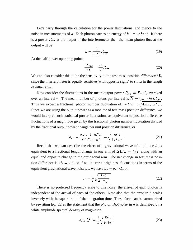
Let’s carry through the calculation for the power fluctuations, and thence to the

noise in measurements ofh. Each photon carries an energy of�h! = 2��hc=�. If there

is a powerPout at the output of the interferometer then the mean photon flux at the

output will be

�n =�

2��hcPout: (19)

At the half-power operating point,

dPout

dL=

2�

�Pin: (20)

We can also consider this to be the sensitivity to the test mass positiondifference�L,

since the interferometer is equally sensitive (with opposite signs) to shifts in the length

of either arm.

Now consider the fluctuations in the mean output powerPout = Pin=2, averaged

over an interval� . The mean number of photons per interval isN = (�=4��hc)Pin� .

Thus we expect a fractional photon number fluctuation of� �N= �N =q4��hc=�Pin� .

Since we are using the output power as a monitor of test mass position difference, we

would interpret such statistical power fluctuations as equivalent to position difference

fluctuations of a magnitude given by the fractional photon number fluctuation divided

by the fractional output power change per unit position difference, or

��L =�N

N=

1

Pout

dPout

dL=

s�hc�

4�Pin�: (21)

Recall that we can describe the effect of a gravitational wave of amplitudeh as

equivalent to a fractional length change in one arm of�L=L = h=2, along with an

equal and opposite change in the orthogonal arm. The net change in test mass posi-

tion difference is�L = Lh; so if we interpret brightness fluctuations in terms of the

equivalent gravitational wave noise�h, we have�h = ��L=L, or

�h =1

L

s�hc�

4�Pin�: (22)

There is no preferred frequency scale to this noise; the arrival of each photon is

independent of the arrival of each of the others. Note also that the error inh scales

inversely with the square root of the integration time. These facts can be summarized

by rewriting Eq. 22 as the statement that thephoton shot noisein h is described by a

white amplitude spectral density of magnitude

hshot(f) =1

L

s�hc�

2�Pin

: (23)

4.2.3 Radiation pressure noise in an interferometer

A hint at where quantum mechanics might have some deep relevance comes when we

consider how shot noise scales with the optical power used in the interferometer. As

shown in Eq. 23 above, the shot noise readout precision improves as the square root

of the optical power. Taken at face value, this would suggest that we could achieve

arbitrarily good measurement precision, so long as we were able to use an arbitrarily

powerful laser to illuminate the interferometer.

That conclusion is encouraging, but ought to cause some unease. After all, didn’t

Einstein fail to find a way to defeat the Uncertainty Principle’s limit to the precision of

mechanical measurements?17 Or did he just blunder not to consider using an interfer-

ometer to make the measurements?

Of course not. An interferometer is in fact very much like the “Heisenberg micro-

scope” of Bohr. The lesson we should draw from that example is that we must not

neglect the effects of recoil in an interferometer. In effect, an interferometer with free

masses is a Heisenberg “macroscope”: the role of the small object whose position is to

be determined is played by the set of macroscopic test masses. Their large size gives

an obvious advantage against recoil, but can’t make the effect vanish entirely.

The recoil effect does have one extra bit of subtlety, though. Recall that the mea-

surement we make in a Michelson interferometer has to do with the difference in length

of the two arms. So the recoil force we need to calculate is not the common mode force

(the component that is equal in the two arms), but only the noise in the difference of the

recoil forces in the two arms. If we use a naive picture in which photons independently

choose which arm to enter, then the origin of a differential recoil force noise is clear.

Each photon enters either one arm or the other; whenever one arm gains a photon, the

other loses one.

To estimate the size of this effect, first recall that the force exerted by an electro-

magnetic wave of powerP reflecting normally from a lossless mirror is

Frad =P

c: (24)

The fluctuation in this force is due to shot noise fluctuation inP . That is

�F =1

c�P ; (25)

or, in terms of an amplitude spectral density

F (f) =

s2��hPin

c�(26)

independent of frequency.

This noisy force is applied to each mass in an arm. For now, let us consider a simple

“one-bounce” interferometer. We will allow the mirrors at the ends of the arms to be

free masses, but in this example assume that the beam splitter is much more massive

than the other mirrors. The fluctuating radiation pressure from the powerPin=2 causes

each mass to move with a spectrum

x(f) =1

m(2�f)2F (f) =

1

mf 2

s�hPin

8�3c�: (27)

The power fluctuations in the two arms will be anti-correlated. The radiation pressure

noise is then

hrp(f) =2

Lx(f) =

1

mf 2L

s�hPin

2�3c�: (28)

4.2.4 The standard quantum limit

Thus we have two different sources of noise associated with the quantum nature of

light. Note that they have opposite scaling with the light power – shot noise declines as

the power grows, but radiation pressure noise grows with power.

If we choose to, we can consider these two noise sources to be two faces of a single

noise that we can call optical readout noise, given by the quadrature sum

ho:r:o:(f) =qh2shot(f) + h2rp(f): (29)

At low frequencies, the radiation pressure term (proportional to1=f 2) will dominate,

while at high frequencies the shot noise (which is independent of frequency, or “white”)

is more important We could improve the high frequency sensitivity by increasingPin ,

at the expense of increased noise at low frequency. At any given frequencyf0, there is

a minimum noise spectral density; clearly, this occurs when the powerPin is chosen to

have the valuePopt that yieldshshot(f0) = hrp(f0).

When we solve forPopt and insert it into our formula forho:r:o: we find

hQL(f) =1

�fL

s�h

m: (30)

We have renamed this locus of lowest possible noisehQL(f), for “quantum limit”, to

emphasize its fundamental relationship to quantum mechanical limits to the precision

of measurements. Note that the expression does not depend onPin or �, or any other

feature of the readout scheme, even though such details were useful for our deriva-

tion. Thus, this examination of the workings of our Heisenberg microscope provides an

instrument-specific derivation of Heisenberg Uncertainty Principle. And it reminds us

of the truth Bohr’s remarks expressed, that in any measurement the Uncertainty Princi-

ple emerges from the specific mechanism of the measurement.

There was a moment when some physicists believed, on seemingly sound physical

grounds, that this picture of how photons interact with a beam splitter was so flawed

that interferometers could perhaps evade the Uncertainty Principle.18 The argument can

be made based on quotation from quantum mechanical Scripture, Dirac’sThe Princi-

ples of Quantum Mechanics.19 There one can read that photons in an interferometer

travel down both arms simultaneously; furthermore, it is written that interference can

only take place between a photon and itself, so the very existence of interference in

a quantum mechanical world is proof of this picture. If this were taken as absolute

and literal truth, then it would appear to rule out any differential radiation pressure at

all, since the number of photons, and hence the recoil forces, would be identical in the

two arms. Without the resulting differential recoil of the test masses, there is no quan-

tum limit. Gravitational waves could in principle be measured with arbitrary precision.

Some physicists defended this as gospel, despite the fact that the argument appeared to

use quantum mechanical reasoning to disprove quantum mechanics.

The stubbornly naive were untroubled by this argument, and expected the Uncer-

tainty Principle to hold. Some physicists read a few pages farther in Dirac’s book, to

the passage explaining that allowing the possibility of energy measurements, say by

observation of recoil of the mirrors, causes collapse of the wave function in such a way

that photons end up either in one arm or the other.(Dirac’s first discussion refers to an

interferometer with rigidly fixed mirrors.) The learned were saved from error by the

work of Caves,20 who invoked the concept of vacuum fluctuations to explain the quan-

tum mechanical behavior of photons at a beam splitter. A vacuum electromagnetic field

with zero-point fluctuations enters the interferometer through the output port; its super-

position with the field from the laser causes the light to behave in the way expected

from semi-classical reasoning.

4.3 Seismic noise

We have neglected to consider above another source of noise in gravitational wave de-

tectors that is so common and important as to be essentially ubiquitous. This is what is

commonly called seismic noise, the continual shaking of the terrestrial environment due

to a variety of contingent causes, ranging from small earthquakes to ocean waves driven

by large weather systems to automobiles striking potholes in poorly paved streets. Such

a complex phenomenon can have no simple explanation from basic physics, yet dealing

with it forms a substantial part of the challenge to designers of gravitational wave de-

tectors. (Only moving the whole detector into space suffices to remove it entirely from

consideration.)

At a reasonably quiet location, the spectrum of seismic noise from 1 Hz to several

hundred Hz can be approximated as

x(f) =

(10�7cm=

pHz; from 1 to 10 Hz

10�7cm=pHz(10Hz=f)2; for f > 10 Hz.

(31)

The magnitude of this mechanical noise background is distressingly large. The rms

amplitude of the noise over this interval is of order 1�m. The good news is that

the spectrum falls with increasing frequencyf . But even so, throughout the range of

frequencies of interest to gravitational wave detectors it involves motions many orders

of magnitude larger than would be driven by any conceivable incident gravitational

wave. There is no possibility of success unless the effects of seismic noise can be

strongly attenuated.

It is straightforward to see the way in which seismic noise mimics a gravitational

wave signal in an interferometer. As long as the separation between the mirrors is

not very small, then the seismic inputs to each mirror are effectively independent; the

difference in arm lengths is driven by quadrature sum of the noise at all mirrors. The

situation is a bit more subtle for a resonant mass detector. If it is suspended at its

midpoint, it would appear that its internal modes should not be excited by any motion

of the suspension point. However, this argument assumes perfect symmetry of the

resonator about the suspension. The approximate symmetry of real systems may give

several orders of magnitude of effective isolation, but the seismic spectrum is so large

that additional isolation is always required.

Fortunately, the design of seismic isolators is a well-developed art. One can con-

struct mechanical multi-pole low-pass filters that provide outstanding attenuation at

frequencies well above those of the filter poles. The art of doing so was introduced to

the field of gravitational wave detection by the founder, Weber.21

4.3.1 A simple two-pole isolator

The essence of vibration isolation can be understood using only ideas from freshman

physics. Imagine that the object to be isolated has massm. Assume that it is a rigid

body, and that we are only interested in its motionxm in a single direction. Then we

can treat the object as a point mass. If it rests on the ground, it shares the ground’s

motionxg, soxm = xg. To isolate the mass, replace the rigid connection to the ground

with a compliant connection, that is attach it to the ground through a spring with spring

constantk. Then the equation of motion of the mass is

m�xm = �k(xm � xg): (32)

With the usual frequency domain ansatzxm(t) = xm exp (i!t), xg(t) = xg exp (i!t),

Eq. 32 can be solved for the vibration transfer function

xm

xg=

!2

0

!20 � !2

; (33)

where!2

0� k=m. The asymptotic behavior of Eq. 33 reveals the essential features of

an isolator – although for low frequencies! � !0, xm=xg � 1 (the mass moves rigidly

with the ground), at high frequencies! � !0, xm=xg � !2

0=!2 (the amplitude of the

mass’s motion falls steeply with increasing frequency.)

(The transfer function of Eq. 33 has the unphysical feature that it predicts an in-

finite response at the resonant frequency!0. This problem is remedied if we add a

damping force to our oversimplified model. Even so, an isolator does have the unfortu-

nate feature that it gives a resonant amplification of the input noise for frequencies near

!0.)

So, a strategy for isolation is as follows: to isolate an experiment for signal fre-

quency!, construct an isolator with a low enough resonant frequency!0 so that the

isolation factor!2

0=!2 is sufficiently small to reduce the seismically driven value ofxm

to a tolerable level.

4.3.2 Isolation stacks

If it proves difficult to make!0 sufficiently low (it often does), another straightforward

idea can often be made to work instead. Make two or more isolators with resonant

frequencies as low as is convenient, then cascade them with the system you want to

isolate farthest from the noisy ground. Solving for the resonant frequencies of the

coupled chain of isolators is a normal mode problem that may get complicated. But

the high frequency limit of a chain ofN isolators, each with resonant frequency!0 by

itself, has the simple formxm

xg� !2

0

!2

!N

: (34)

In Weber’s original experiment, a vibration isolation “stack” of alternating steel

plates and rubber sheets was used. No details are given in the text of his papers, but the

idea was clear, and was adopted by those who followed Weber as well. Among the nice

features of this isolator are: rough equality of the isolation in all degrees of freedom

(since the rubber is compliant in both compression and in shear), and a small level of

resonant amplification (since the rubber is rather lossy).

4.3.3 Isolation for interferometers

The pendulum that provides a low-dissipation suspension for the test mass in an in-

terferometer also provides two poles of seismic isolation. Typically, the resonant fre-

quency is close to 1 Hz. This single stage might almost provide enough isolation for

gravitational wave measurements in the vicinity of 1 kHz, but certainly requires sub-

stantial augmentation for good sensitivity at lower frequencies. This additional isola-

tion needs to be at least roughly isotropic, since there are a variety of cross-coupling

mechanisms that can make vertical noise couple to the phase of the light beam.

The simplest way to add isolation is to suspend the pendulum from a stack of the

sort used to isolate a resonant-mass detector. Since interferometers are usually aimed

at having good sensitivities down to the lowest possible frequencies, there is a strong

incentive to make a stack with the lowest possible resonant frequencies.

More dramatic re-engineering of the basic stack concept can yield greater rewards.

The strongest effort in this direction has been made by the VIRGO group in Pisa.22 The

basic idea is to build a stack based on many cascaded pendulums, but to build enough

vertical compliance into each pendulum stage to give effective vertical resonant fre-

quencies comparable to the 1 Hz resonances of the pendulum stages. In its original

version, the vertical springs were air springs made of flexible bellows. This yielded im-

pressive performance, which was improved even further when the vertical compliance

was enhanced by magnetic anti-springs arranged to cancel some of the vertical stiff-

ness. The original version would have made seismic noise negligible (compared with

shot noise) for all frequencies above 10 Hz, while the enhanced version would work

down to 4 Hz. The air springs did suffer from one serious drawback; the temperature

coefficient of the spring force is determined by the ideal gas law, a much stronger sensi-

tivity than elastic springs. Drifts proved very hard to control. To remedy this problem,

the system was completely redesigned, with the air springs replaced by pre-stressed

steel cantilevers in the form of narrow triangular blades, supplemented with magnetic

anti-springs.

4.4 Noise in resonant-mass detectors

Key features The essential complication in understanding resonant-mass detectors

(as compared to interferometric detectors) is that the degree of freedom of interest is

that of a simple harmonic oscillator (or a collection of them, as we’ll see in the next

section.) So in addition to any intrinsic frequency dependence in the noise, there is

a deliberately constructed resonant transfer function in the detector itself. As we saw

earlier in this review, the resonance was introduced as part of a strategy for overcoming

wide-band noise in the amplifier.

The use of this strategy involves different heuristic concepts than are appropriate

for interferometers. In particular, optimizing the sensitivity of a resonant detector to

short bursts almost always involves choosing to average the output over times that are

long compared with the length of the burst itself. Then, the measurable quantity is no

longerh(t), but is instead net change in the vector amplitude (magnitude and phase)

of the resonator’s oscillation. This in turn can be expressed in terms of the energy that

the wave would have deposited in a resonator at rest.23 If the gravitational waveform

h(t) has a Fourier transformH(f), then that excitation energyE is (for an optimal

orientation between bar and wave)24

E =Mv4sL2

jH (f0)j2 ; (35)

whereM is the total mass of the bar,vs is the speed of sound in the material,L is the

overall length of the bar, andf0 is the resonant frequency.

The distinctive features are twofold: characterization of all candidate events by a

single number (usually its ”energy” or elseT � E=kB), and a signal-to-noise optimiza-

tion that involves choosing the right averaging time (or bandwidth).

Resonant transducers The second generation of resonant-mass detectors replaced

Weber’s piezoelectric transducer with a kind of a bridge circuit, in which the mechan-

ical motion unbalanced the bridge by modulating the inductance or capacitance of one

leg of the bridge. As with piezoelectric transducers, achieving a high level of coupling

has proven difficult to achieve. A standard measure of the coupling is the Gibbons-

Hawking parameter�, defined as “the proportion of elastic energy of the detector that

can be extracted electrically from the transducer in one cycle.”25 In principle, the exci-

tation of the bridge could be increased without limit, but in practice large fields usually

lead to excess dissipation in the transducer even before electrical breakdown occurs.

Transducers have been limited to working values of� of around 10�2.

A heuristic way of understanding the design problem is to think of the issue as

an attempt to design a transducer that makes a reasonable electrical impedance at its

output appear to the mechanical system as a mechanical resistance sufficient to supply

appreciable damping to the bar. With bar masses in excess of 1 ton, this may seem

inordinately difficult. The good values mentioned in the previous paragraph avoided

this problem by making use of so-called resonant transducers, which have been adopted

almost universally since the idea was proposed by Paik in 1976.26

Paik’s design called for a smaller mechanical resonator to be attached to the main

resonant massM . The resonant frequency of the smaller resonator itself (i.e. with the

larger resonator “clamped”) is chosen to match that of the main resonator. The actual

coupled system then has two normal modes. If the mass ratiom=M � � � 1, then it

is easy to show that the ratio of the amplitude of motion of the small mass, compared

with that of the main resonator, is ���� xX���� = 2p

�:

When a gravitational wave burst interacts with such a resonant system, it will at

first mainly excite the vibration of the large bar. (The Paik resonator is a small device

at one end of the bar, so the gravitational wave strain has only a small baseline for

creating a stretch in its spring.) The free motion of this two-mode system then exhibits

“beats”, during which the mechanical energy of the main resonator’s original motion is

transferred into excitation of the small resonator. During this phase of the beat cycle, the

effect of the gravitational wave has been transformed into a motion2=p� times larger

than in a detector without the resonant transducer. The electro-mechanical transducer

is mounted so as to measure the motion of the small mass with respect to the end of the

main resonator, thus presenting this larger motion to the rest of the signal processing

system.

The advantage this offers in detecting weak signals is probably obvious. The larger

motion generates a comparably larger electrical output from the transducer, reducing

the importance of a given level of electrical amplifier noise. Another way of seeing the

advantage is to recognize the much smaller mechanical impedance required to damp

the motion of the smaller mass, which means that� is increased by a factor of order

��1. In present day designs, the mass ratio� is typically of order a few times10�3.

The value is set in an optimization that involves not only thermal noise and additive

amplifier noise but the back-action noise as well.

4.4.1 Thermal noise in resonant-mass detectors

Even though resonant-mass detectors work in a rather different way than free-mass

detectors, they still benefit from low levels of dissipation. Here, one makes exactly the

opposite design choice in regard to the resonant frequency – rather than trying to put all

resonances outside the signal band of interest, the whole detection strategy is based on

placing the resonance at a frequency where one expects signal power to be large. So, on

the face of it, all of the12kBT of energy contributes to the rms scatter of the instrument’s

output. But it would be too hasty to conclude that there is no dependence of the effective

thermal noise on the disspation level. The typical resonant-mass detector can have

a damping time of order 1000 sec, while the resonant frequency is near 1 kHz (i.e,

a quality factorQ of order106.) The signal being sought might be a brief burst of

radiation, lasting only a millisecond. In this brief interval, the bar’s amplitude and/or

phase of oscillation are altered. The characteristic time for such changes due to thermal

noise is the damping time. So only a small fraction of the thermal noise power is

relevant in the detection process. For this reason, low dissipation can be as valuable in

resonant-mass detectors as in interferometers.

To make the analogy with free-mass detectors clearer, we can make a frequency

domain version of the argument in the previous paragraph. It is most convenient to

consider the comparison between the thermal noise driving force, Eq. 14, and the force

exerted by the gravitational wave on the detector. A brief burst of gravitational waves

will have a broad spectrum; its matched filter will admit power over a wide band. The

thermal noise force power spectrum that may obscure the effect of the gravitational

wave is broad-band as well; if the dissipation in the bar has the form of velocity damp-

ing, then the spectrum is white. The amplitude of this broad band noise spectrum is

proportional to the amount of dissipation. So the signal to noise ratio will be better, the

smaller is the amount of dissipation.

An expression for the minimum detectable noise�Emin (at the 1� level) is27

�Emin � 2kBT�s

�d; (36)

whereT is the temperature,�s is the averaging time, and�d is the damping time of the

bar. In this case (where we assume only thermal noise is important), it is clear that the

shorter the averaging time the better the sensitivity.

4.4.2 Readout noise in a resonant-mass detector

Most of the issues of readout noise discussed above for interferometers were first faced

in the context of resonant-mass detectors. We have inverted the historical order solely

for pedagogical reasons; the physical origin of readout noise in an interferometer is

transparent, and nominally free masses make a more straightforward analogy to the

Heisenberg microscope than does the complex amplitude of a resonant mode. A key

role was played by Braginsky28 in calling attention to necessity of understanding these

issues in resonant-mass gravitational wave detectors.

Transducer model The transducer is treated as a black box, in the form of a two-

port network, emphasizing the fact that the system has a single input port and a single

output port. Unlike the two-ports usually studied in electrical engineering classes, the

transducer changes the dimensions of the signal: a mechanical motion at the input is

converted to an electrical signal at the output.

One such device is a seismometer pickup: a permanent magnet attached to the end

of the bar, arranged so that it moves back and forth in the vicinity of a conducting coil

whenever the bar vibrates. Motion of the mechanical system generates an electromotive

force in the coil that can be electrically amplified and recorded.

In gravitational wave detectors, the transducers usually involve a reactance (i.e. an

inductance or a capacitance) whose value is modified by relative motion between the

transducer mass and the end of the bar. This generates an electrical signal by virtue of

the fact that the reactive component is placed in one leg of a bridge circuit. This kind of

transducer is a passive device. It can add noise if its level of dissipation is large enough

so that thermal noise is important.

There has also been development of parametric transducers, in which a balanced

bridge (two counter-varying reactances) is excited at microwave frequencies. This is

the kind of transducer used on the UWA detector.29 There is a deep analogy between

this kind of transducer and an interferometer.30 This means that there are both extra

benefits (gain in the transducer) and extra complications (such as noise in the oscillator

that excites the bridge.)

Pre-amplifier The remaining essential part of the readout system is the low noise

pre-amplifier, whose job is to transform the tiny electrical output of the transducer into

a signal large enough so that it can be recorded. One needs the noise to be as low as

possible. To describe the noise, and to understand how it affects the detection process,

is valuable to consider a general black box representation of a noisy amplifier as a kind

of a two-port network, just as we did for the transducer. Other than the trivial difference

that this two-port is an all-electric device, there are two key differences between this

kind of two-port and the model transducers discussed above. One is the fact that the

amplifier has gain, i.e. it can supply more energy at its output than is supplied by its

input. The other is the existence of two sources that represent the generation of noise.

They are usually represented as a voltage source and a current source at the input of

the two-port network; this is especially convenient, and has wide generality, but is only

one of several equivalent ways of representing the noise. More on the general theory of

noisy two-port networks can be found in the pioneering paper by Rothe and Dahlke.31

It is interesting to pause to inquire why two noise sources are necessary. Recall

the Helmholtz theorem, often known in specialized forms as Th´evenin’s theorem or

Norton’s theorem.32 The essence of the theorem is that an arbitrary network of sources

and passive components can be represented, as far as its behavior at a given port is

concerned, by a single source and a single impedance. But we are dealing here with a

network in which two ports are relevant. At each port, one needs an impedance and a

source, or their equivalents elsewhere in the circuit. It is traditional to replace the source

at the output with an equivalent noise source at the input, whose strength is smaller than

the output noise by a factor of the amplifier gain.

These two noise sources play different roles in the measurement process. There

is one noise source that is physically present at the input, causing an influence on the

system (here the electromechancal transducer) that is attached to the amplifier input. In

the jargon of gravitational wave detection, this noise is responsible for “back action”,

since noise at the input of the pre-amp is thereby applied to the output end of the trans-

ducer,where it can cause a mechanical noise force at the transducer input; this is in turn

attached to the resonant-mass detector proper. More on this below.

The second noise source (the one replacing the output noise source) is usually re-

ferred to as “additive noise”: it is added to the amplified signal by the time it appears at

the output, without causing any physical effect on the system hooked up to the input.

Amplifier noise in resonant-mass gravitational wave detectors, and the “amplifier

limit” In contrast to our discussion of detection strategies in the case where thermal

noise dominates, we here discuss the case when additive amplifier noise is the only

important noise source. Then, we can best search for a brief burst of gravitational

radiation by performing a cross-correlation between the system output and a template

consisting of a sinusoid at the mechanical resonant frequency that is damped with the

same time constant as the resonance itself. In other words, we look for responses that

look like the test mass system suddenly set into resonance. The signal can arrive with

any phase of course, so we need to keep track of both sine and cosine components with

the bar’s damping time. A two-phase lock-in amplifier can be set up to perform exactly

this form of averaging.

In this case the energy sensitivity of the detector is given by27

�Emin � kBTn�+ ��1

���sf0; (37)

whereTn is the noise temperature of the amplifier,� is the ratio of the transducer

output impedance to the amplifer noise impedance,� is the Gibbons-Hawking coupling

parameter, and�s is the averaging time.

Consider the post-detection bandwidth implied by this prescription. The output of

the cross-correlation described above is hardly affected if we displace the template with

respect to the signal time series by one or even several cycles of oscillation. For there

to be a substantial change in the value of the cross-correlation, the template must be

displaced by a duration of order the damping time of the mechanical resonance. This

means that, if the signal-to-noise ratio is not large, the arrival time of the impulsive

gravitational wave signal will be uncertain by of order the damping time. In other

words, the post-detection bandwidth�f of such a signal extraction system is narrow,

of order

�f � 1=�d:

For a a quality factor of106, this bandwidth is very narrow indeed. Increased bandwidth

could be achieved, of course, at the expense of the signal-to-noise ratio, by averaging

the output time series for a shorter time than the bar’s damping time�d.

Combined optimum in the presence of thermal noise and additive amplifier noise

When both kinds of noise are present at substantial levels, the best strategy is neither

the rapid readout appropriate to thermal noise nor the long averaging time that would

be best for amplifier noise. A broad-band output filter will admit too much amplifier

noise. Using the narrow-band prescription appropriate to the amplifier-dominated case

filters out much thermal noise, but also most of the signal power. Obviously, the opti-

mum in the combined noise case lies somewhere between the extremes, where the net

noise contributions from thermal noise and amplifier noise are equal. Then, the energy

sensitivity of the detector is given by27

�Emin � 2kBT�s

�d+ kBTn

�+ ��1

���sf0; (38)

where the averaging time is now to be chosen in such a way as to minimize the sum of

the two terms.

The larger is the transducer’s coupling�, the smaller is the importance of amplifier

noise in units of gravitational wave strength. In the limit of large�, the bandwidth of

resonant-mass gravitational wave detector can approach that given by the thermal noise

limit, where the matched template is the signal waveform itself.

For detectors with resonant transducers, bandwidth is also limited by the splitting

between the coupled modes of the bar-transducer system. There is a competition be-

tween two effects: a small transducer mass gives a large mechanical amplification but a

small mode splitting. In the time domain, this would be described as a long beat period;

after a signal excites the bar one has to wait for a substantial fraction of the beat period

for energy to be transferred to the motion of the transducer mass. This competition

could be evaded by the construction of multi-mass transducers with a gradation from

intermediate to tiny masses.33

Resonant-mass gravitational wave detectors built to date have almost always been

substantially under-coupled to their amplifiers. First-generation bars of Weber’s type,

in which the transduction was performed by piezoelectric transducerss glued around

the belly of the cylindrical mass, could only achieve coupling factors of order5�10�6.

One variant constructed by the Glasgow group did achieve a large�.34 It consisted of a

cylindrical bar that had been split in half, then reassembled with a layer of piezoelectric

material in effect forming the spring attaching the masses at either end. This design is

the closest approach ever to Weber’s original vision of a single massive piezoelectric

mass as an antenna. In spite of these impressive parameters, the Glasgow bar was

never even the most sensitive gravitational wave detector of its day, because the poor

mechanicalQ of the piezoelectric material gave a large amount of thermal noise.

4.4.3 The quantum limit in resonant-mass detectors

One of the key features of Rothe and Dahlke’s model of a noisy two-port network is the

necessity to describe the noise with two generators, one directly limiting measurement

precision and the other disturbing the system being measured. This is reminiscent of

concepts most students of physics learn about in the context of quantum mechanics. In

fact, quantum mechanics sets a minimum level of amplifier noise that can be expressed

in terms of this pair of noise generators.

Quantum mechanical noise in an electrical amplifier A paper by Heffner in 1962

derived the quantum mechanical limit on amplifier noise;35 its relevance for the grav-

itational wave detector problem was discovered by Giffard in 1976.36 What Heffner

showed was that, unless an electrical amplifier had a minimum level of noise, it could

be used to make measurements of an electrical signal at frequencyf that evaded the

Uncertainty Principle

�n�� � 1

2;

where�n is the uncertainty in the number of photons at the frequencyf , and�� is the

uncertainty in the measurement of the phase of the signal.

The amplifier noise that just barely allows measurements at the Uncertainty Princi-

ple limit is given by

qSv(f)Si(f) =

ln

2� 1=G

1� 1=G

!�1

2��hf:

In the limit of large gainG, this limit becomesqSv(f)Si(f) =

1

ln 22��hf: (39)

The combination of voltage and current noise power spectra represents yet another pair

of conjugate variables governed by an uncertainty relation. This product is proportional

to the noise temperatureTn of the amplifier, defined bykBTn �qSv(f)Si(f).

In the earliest days of the search for gravitational waves, the possible implications

of such an amplifier sensitivity limit for the sensitivity of gravitational wave detectors

were ignored. Neither Weber’s papers nor the canonical theoretical analysis by Gibbons

and Hawking mention such a limit. Eventually, cooler heads came to contemplate the

fact that gravitational wave detectors ought to obey the Uncertainty Principle.

The electro-mechanical Uncertainty Principle Giffard gave the adaptation of this

argument to the electro-mechanical case. His argument is so brief that it is almost hard

to state. He points out that the functions of transducer and pre-amplifier together can

be thought of as a so-called “mechanical amplifier”, a two-port network whose input

terminal receives a mechanical signal, but whose output is electrical.

From this, Giffard shows that the Uncertainty Principle requires that unless a grav-

itational wave signal has a minimum size, no linear gravitational wave detector will be

able to register its arrival. He expressed the minimum size in terms of the energyUs that

the wave would deposit in a resonant detector initially at rest. The quantum mechanical

limiting sensitivity is

Us > 4��hf:

As worded above, this argument can seem rather abstract. A heuristic description

makes it as vivid as any of Bohr’sgedankenexperiments. In a mechanical amplifier,

a crucial quantum mechanical role is played by the back action from the noise source

that the Helmholtz Theorem places at the amplifier input. The force noise generator

at the mechanical amplifier input (caused by electrical noise acting backwards through

the transducer) perturbs the delicate mechanical system, here the resonant-mass system

itself. Just as in the Heisenberg microscope, any design trade-off made in an attempt

to reduce the position noise ends up increasing the momentum impulse applied to the

system being measured.

5 History of resonant-mass detectors

We now turn from a discussion of physicsper seto a review of the way in which

one assembles working gravitational wave detectors in light of the physical principles

governing them. We will take a quasi-historical framework for this discussion, as a

pedagogically sensible way of grappling with the issues involved. In this section, we

will take the chronologically-motivated choice of treating resonant-mass detectors first;

then we will start from scratch the overlapping history of interferometric detectors.

By 1966, Joseph Weber had constructed a complete working detector, and by 1968

was reporting coincident observations between detectors separated by 1000 km. The

detector contained versions of every essential feature in resonant-mass gravitational

wave detectors today, except for the facts that it operated at room temperature and that

it used non-resonant strain transducers for its readout. The story of the development of

the field since then can be seen as embodying a few key accomplishments: replication

of Weber’s detectors accompanied by a failure to confirm his claimed detection, clarifi-

cation of the optimum way to detect gravitational wave signals in a noisy detector and

of the sorts of technological developments that could lead to improved detector sensi-

tivity, and the staged implementation of new generations of detectors embodying the

improved technology.

5.1 Weber’s detectors as gravitational-wave detection systems

All of the important elements that make up a working gravitational wave detector are

described in Weber’s 1966Physical Review Letter.21 Looking at the signal chain from

the front end, we see first the large 11

2ton aluminum cylinder whose fundamental lon-

gitudinal mode at 1657 Hz interacts with any incoming gravitational wave. Around

its midsection are glued the quartz transducers that give, through the piezoelectric ef-

fect, electrical signals proportional to the strain in the aluminum cylinder. Signal leads

from those transducers pass through acoustic filters and through the wall of the vacuum

chamber, then are connected via another acoustic filter to a superconducting inductance

that serves as a “tank circuit” at the input of the low-noise pre-amplifier (whose noise

temperature is 50 K.) The output of the pre-amp is connected to further amplification.

There follows a rectifier for generating a positive-definite signal proportional to the

power out of the amplifier. The end of the signal chain is a recording device, which in

1966 consisted of a pen-and-ink chart recorder.

Another aspect of the detector is the means used to prevent its being excited by

influences other than gravitational waves. Isolation against mechanical influences in

the form of acoustic or seismic noise is shown clearly in the diagram. Direct acoustic

excitation is prevented by the placement of the key parts of the experiment inside a

vacuum chamber. Transmission of vibration through the signal leads is attenuated by

the acoustic filters mentioned above. The path for vibrations from the floor must pass

through a pair of isolation stacks each consisting of three stages of rubber pad / steel

block isolators; the aluminum bar is further isolated by a pendulum suspension consist-

ing of a single wire sling that supports the bar about its middle. The top ends of the

wire are attached to a beam that spans the space between the isolation stacks.

Further progress in reducing the sensitivity of his bar to spurious external influences

enabled Weber to make his 1969 claim of “Evidence for discovery of gravitational

radiation”.8 One aspect of this progress consisted of augmenting the electromagnetic

shielding of his devices, after tests revealed some sensitivity. A seismometer array was

also used to check for correlations between strong vibration of the ground and large

detector outputs. But by far the most important system element in this regard was the

construction of multiple copies of the complete detector system, and their deployment

at spatially separated locations. The network in 1969 consisted of one bar of 66 cm

diameter and 153 cm length (for a resonant frequency of 1657 Hz) located at the Ar-

gonne National Laboratory in Illinois, and five other resonant-mass detectors located at

the University of Maryland. One bar at Maryland, whose properties matched closely

the Argonne bar, was used together with it to look for coincident excitation. Some use

of the outputs of the additional bars was made, but the procedure is poorly described.

5.2 Weber’s observational program

Weber’s ongoing research program was concerned with looking for further evidence

that the coincident events were real (i.e. not statistical accidents) and that they were

in fact due to gravitational radiation. A Physical Review Letter of 9 February 197037

discusses the statistics from several interesting points of view. The claim that the events

are real is buttressed by calculation of the rate of accidental coincidences. For the whole

range of threshold levels considered, the number of coincidences exceeds the expected

accidental rate by about an order of magnitude. Another even more convincing piece

of evidence comes from carrying out a search for coincidences between the output of

the two detectors using a scheme in which one of the detectors’ outputs was delayed

by two seconds, enough to remove any correlation due to excitation by gravitational

wave impulses. Just as one would hope, only a small number of coincidences occurred

between the offset data streams, at a level consistent with accidentals.

Still another convincing piece of evidence was revealed in a Phys. Rev. Letter of

20 July 1970.38 In it, Weber uses the classic astronomical test of testing for correlation

of his event rate with sidereal time. Jansky’s claim for the extraterrestrial origin of his

observed radio noise had been buttressed in just this way; more recently, Jocelyn Bell

had convinced her reluctant thesis advisor Hewish of the extraterrestrial nature of her

pulsar signals by a similar test. Weber took advantage of the fact that the response of a

cylindrical bar is anisotropic, and that the axes of his bars were oriented East-West, so

that their sensitivity pattern was swept across the sky by the rotation of the Earth. The

histogram of events vs. sidereal time reveals a substantial anisotropy (of order a factor

of two) that peaks when the right ascension of the galactic center crosses the meridian

at the mid-point between Maryland and Argonne, and again 12 hours later (as would be

expected from the symmetry of the antenna pattern and the transparency of the Earth to

gravitational waves.) A similar histogram plotting coincidences against the solar time

of their occurrence is flat within statistical errors.

One disturbing consequence follows from this observation, if one adopts the natu-

ral hypothesis that the sidereal anisotropy indicates that gravitational wave events are

originating in the galactic center. Making other reasonable assumptions about the band-

width of the signals, Weber is led to the conclusion that perhaps as much as 1000M�

per year is being converted into gravitational waves. It is not clear what to make of

the inference that the galaxy would be entirely consumed in much less than a Hubble

time at such a rate of gravitational luminosity. Weber mentions as possible ways out

anisotropic emission from the sources (or focussing of the waves) in such a way that

we see higher than average flux, or the possibility that his detector is not working in

a linear regime, but is instead being stimulated by very weak gravitational waves to

release energy stored in metastable states.

5.3 Early response to Weber’s claims

Weber’s claims attracted a great deal of attention. The experimental evidence appeared

very strong. The problems with the energetics of the events could be taken as a strong

counter-argument, but they could also be interpreted as a demonstration that a truly

remarkable discovery was being made. The review “Gravitational-Wave Astronomy”

by Press and Thorne in 1972’sAnnual Reviews of Astronomy and Astrophysics39 gives

testimony to the significance that was attributed to Weber’s claims, with its extensive

bibliography (completed in December 1971) of papers grappling both with the theo-

retical consequences of Weber’s claims and with experimental ways to improve upon

the sensitivity of Weber’s detectors. The perceived stakes in the controversy are shown

by the three-paragraph introductory section, which is mostly devoted to balancing the

possibility of breakthroughs in the making against the alternative that Weber’s results

are mistaken. This first section concludes with a paragraph, remarkable in a review

article, questioning the very urgency of its subject:

We (the authors) find Weber’s experimental evidence for gravitational waves

fairly convincing. But we also recognize that there are as yet no plausible

theoretical explanations of the waves’ source and observed strength. Thus,

we feel we must protect this review against being made irrelevant by a possi-

ble “disproof” of Weber’s results. We have done this by relegating to the end

of the article (Section 6) all ideas, issues, and discussions that hinge upon

Weber’s observations.

Both the theoretical speculation about sources and the quest for better ways to de-

tect the waves are in evidence in one of the most influential papers of this or any other

epoch in the search for gravitational waves. Gibbons and Hawking, both renowned

for work rather far removed from experimental physics, wrote in late 1970 the very

practical “Theory of the Detection of Short Bursts of Gravitational Radiation”.25 The

introduction presents Weber’s results as established facts. Section II of the paper dis-

cusses possible sources, discussing with equanimity but at some length the extreme

gravitational luminosities required. The rest of the paper is devoted to the theory of

detecting weak gravitational wave bursts in the presence of noise, and to a clear and

original set of proposals for maximizing the signal-to-noise ratio of detectors. Some of

one’s surprise at the authorship of this paper may be alleviated upon reading the thanks

for insights and ideas given (at two places in the text and in the Acknowledgment) to P.

Aplin of Bristol University, a very original experimentalist who published little on this

subject under his own name.40

Gibbons and Hawking pointed out that Weber’s own treatment of the theory of

gravitational wave detectors, written before he started his observations, had been aimed

at their response to steady sinusoidal signals. As such, it gives a misleading idea of the

value of the high-Q resonance that characterizes Weber-style detectors. This lack was

remedied by Gibbons and Hawking, who (with thanks to Aplin) point out that the low

dissipation of a high-Q system means that the level of thermal noise power is low. They

go on to show that the high-Q resonance is also of crucial importance in minimizing the

effect of Johnson noise in the transducer, here playing the role we would generally call

amplifier noise. (A weakness of this light treatment of amplifier noise is that it leaves

out the back action effects that enforce the Uncertainty Principle.)

As we saw previously, Gibbons and Hawking noted that there is in fact a compe-

tition between these two benefits of low dissipation. To minimize thermal noise, one

wants to integrate the output for as short a time as possible, to give the random walk

of the resonator’s complex amplitude the least opportunity to mask a signal. On the

other hand, the importance of transducer/amplifier noise is minimized by integrating

for as long as practicable, so that the gravitational wave signal competes with as small

a bandwidth of the broadband noise as possible. Gibbons and Hawking showed how

to derive the optimum averaging time that minimizes the total noise from these two

sources. In so doing, they noted that the averaging time depends on the dimensionless

coupling parameter they called�, the definition of which we gave above in Section 4.

For Weber’s detector they give an estimate of� � 5� 10�6.

Gibbons and Hawking go on to note that a large value for� would have two bene-

fits: improving the signal-to-noise ratio by making the gravitational wave signal appear

as a larger electrical signal, while simultaneously changing the balance between and

thermal noise and electrical noise in the direction that causes the optimum sensitivity to

be obtained with shorter integration times. In other words, a larger� would yield better

sensitivity and high bandwidth. To obtain these benefits, they discuss a novel config-

uration, proposed by Aplin, that has come to be known as a “split bar”. It consists of

two large masses (two “ends” of a bar split in half) joined to each other by connection

to either face of a layer of piezoelectric material. The benefit comes from the fact that,

in this configuration, the piezo is actually functioning as the dominant spring in the

system; by storing the bulk of the elastic energy, it is able to produce a larger amount of

electrical energy. (In many ways this harks back to Weber’s original proposal to make

the bar entirely of piezoelectric material.)

Gibbons and Hawking sketch the details of a detector of this sort, in which lead

zirconate titanate (PZT) is substituted for crystalline quartz (used by Weber) because

of its larger piezoelectric coupling constant. Then, in spite of the fact that the thermal

noise power is increased because the piezo is a rather lossy spring, the sensitivity should

be increased by more than a factor of 10 in energy compared with Weber’s detector. At

the same time, the optimum sampling time is shortened to 1 msec, so that more detailed

information can be extracted from the signal.

In passing, Gibbons and Hawking also note that Weber uses a less than optimal way

of searching for gravitational wave events. His definition of an event is a noticeable

increase in the energy in the bar’s fundamental mode. But a gravitational wave impulse

will only increase the energy if it arrives with a particular phase relationship to the bar’s

previous excitation. If the wave arrives with a different phase, the bar’s energy may be

decreased, or the effect may instead primarily change the phase of the bar’s vibration.

They estimate that this means Weber saw only about 1/4 of the events exciting a given

bar. And, since the two bars being used for a coincidence have independent phases, only

(1=4)2= 1=16 of the detectable coincidences would have been registered by Weber’s

technique. This makes the question of the source of the gravitational luminosity that

much more difficult to resolve. But it also means that, if Weber’s results were real, even

more events should be detectable.

Whatever mysteries there may have been regarding Weber’s claims that he was de-

tecting pulses of gravitational waves, if they were true they represented one of the most

important astronomical and physical discoveries of the 20th century. So it is no surprise

that a number of other workers decided to construct gravitational wave detectors. And

quite naturally given Weber’s apparent success, most of these detectors were built quite

a bit like Weber’s. Success looked as if it should come quickly. Although it had taken

Weber about a decade, working alone, to design, build, debug, and operate his detec-

tors, those who wanted to follow the recipe he had developed needed much less time.

As Weber himself described it:41

The scheme that works is not very difficult to set up and costs about $25

000, excluding pay for the senior physicists involved. Once set up, the in-

strumentation has run without problems for a little longer than a year and a

half. Furthermore, the instrumentation requires a skilled technician about a

month to construct. It requires a physicist about two days, starting with an

open vacuum chamber to put crystals on the apparatus and make the neces-

sary adjustments to see coincidences. In view of the relative simplicity of

the working instrumentation, it seems reasonable to suggest that others start

in this way.

A group at Frascati42 built a detector as close to Weber’s as possible, including a

close match with his resonant frequency of 1660 Hz. The Munich group of Billing

and Winkler43 also built a quite similar bar. At Moscow State University, a group led

by Braginsky constructed another bar that matched Weber’s rather closely. At Bell

Labs, Tyson44 began a program of construction along Weber’s lines, with less concern

to match all of his parameters exactly — the resonant frequency of his largest bar was

709 Hz. At IBM Labs, Garwin and Levine45 built a small bar of Weber’s style; they

were convinced that they could improve upon Weber’s statistical methods sufficiently

to make up for poorer noise levels. Aplin,40 on the other hand, began to construct

a split bar along the lines he had suggested to Gibbons and Hawking. Although he

did not succeed in carrying that work through to completion, the idea (and some of

the equipment) was taken up by Drever’s group in Glasgow.34 There were also efforts

started at Reading and Regina, and in addition, the second generation detectors of much

greater sensitivity were planned by groups at Stanford, LSU, and Rome. (More about

these later.)

As Weber had predicted, results began to become available very quickly. Unfor-

tunately, it also soon became apparent that no one else was seeing results that looked

anything like Weber’s. By the time of the 6th Texas Symposium on Relativistic As-

trophysics (held in New York December 18-22 1972),41 several groups were ready to

come forward with claims of null results at sensitivities comparable to or better than

Weber’s. Tyson made the strongest claims for the unreality of Weber’s signals, based

both on his own failure to find them in his single detector (at sensitivities better than

Weber’s) as well as his claims that Weber’s electronics was too noisy even to record

Brownian motion in his bar. Kafka, representing the Frascati and Munich groups (who

performed observations in coincidence), was able to report only preliminary results

(delivered to him by telegram) of five days of observations, but the failure to find any

statistically significant number of coincidences was in strong contradiction to their ex-

pectations if Weber’s claims were correct. Drever also reported negative results from

the high-bandwidth split bar at Glasgow; he, however, tempered his claims of conflict

with Weber by noting that his detector would only be expected to see Weber’s events if

they were of a few milliseconds duration (an assumption that was plausible but by no

means certain.)

5.4 Resolution of the Weber controversy

Over the next year and a half, there was an intensive concentration of effort to attempt

to resolve the controversy. The groups listed above continued to accumulate data, none

of which confirmed Weber’s claim of a substantial flux of strong gravitational-wave

pulses. New negative results from Garwin and Levine of IBM Labs were reported in a

strongly-worded series of articles inPhysical Review Letters.45 Their work was carried

out in the explicit belief that Weber’s results were spurious, and could be shown to be so

by the use of a single detector of well-characterized performance, even if that detector

was small. (The titles of the three articles are miniature masterpieces of polemical style:

“Absence of Gravity-Wave Signals in a Bar at 1695 Hz”, “Single Gravity-Wave De-

tector Results Contrasted with Previous Coincidence Detections”, and “New Negative

Result for Gravitational Wave Detection, and Comparison with Reported Detection.”)

The first results to be reported came from a bar with a mass of 118 kg, the second from

a 500 kg bar. Compare with the mass of Weber’s principal detectors, 1500 kg.

The letters of the IBM group present the statistics of the noise output of their de-

tectors, along with a careful tutorial on the theory of extracting impulsive signals from

noise. This latter theme can be thought of as an explication of the signal processing

scheme proposed (in rather telegraphic style) in Gibbons and Hawking’s 1971 paper.

The key idea was not to rely on net increase in the energy of the bar, but to look for

sudden changes, of either sign, in either the magnitude or phase of the detector’s com-

plex excitation. The thrust of the papers is that if Weber’s results were correct, then

even their less massive single detector ought to show substantial departures from the

Gaussian distribution of excitation expected on the basis of thermal and amplifier noise

alone. The near-perfect Gaussian fit to their data then constitutes an apparent contra-

diction of Weber’s results.

An important argument used to buttress the claim that the IBM detector was well un-

derstood was the application of electrostatic calibration forces to one end of the bar, and

the successful detection of those events (within the statistical limits set by the signal-

to-noise ratio) by the data processing system. Tyson’s 1972 presentation to the Texas

meeting had previously emphasized the importance of this fundamental practice of ex-

perimental physics, as did the remarks of both Kafka and Drever. Levine and Garwin

take Weber to task for having failed to use any calibration method, either as a check of

his instruments’ front ends or of his data analysis procedure.

A more subtle implicit argument against Weber’s work is suggested to the reader

of these papers by their admirable clarity, as contrasted with the rather Delphic pro-

nouncements that fill Weber’s own contributions toPhysical Review Letters. Levine

and Garwin make this explicit at one point when they compare their results with their

best guess at how Weber’s would be expressed in similar (sensible) units, complaining

“We are thus forced to estimate these quantities, while noting that such information is

easily obtained by the experimenter and is normally provided in the publication of a

detection experiment.”46

Garwin led a crusade against Weber’s claims at the Fifth Cambridge Conference on

Relativity (CCR-5), held at MIT on 10 June 1974.47 Among the topics discussed was

1) an error in the computer program used by Weber to identify coincidences, shown to

generate nearly all of the coincidences in the one data tape shared by Weber with other

researchers, and 2) the puzzling feature of Weber’s histogram of coincidences versus

time delay showing a peak at zero delay in only the central 0.1 second wide bin, in

spite of the fact that a 1.6 Hz wide bandpass filter was said to be part of the signal

processing chain. But the most spectacular event of the discussion was what even those

sympathetic to Garwin’s cause might have felt was a trick that bordered on unsports-

manlike conduct. Weber had been given data from the detector of Douglass’s group

at the University of Rochester, to search for excitations in coincidence with Weber’s

own detectors; Weber reported at previous meetings that he had detected an excess of

coincident events at a level of 2.6 standard deviations above the expected chance rate.

According to Garwin’s account in a letter to the editor ofPhysics Today,47 “At CCR-5

Douglass revealed, and Weber agreed, that the Maryland Group had mistakenly as-

sumed that the two antennas used the same time reference, whereas one was on Eastern

Daylight Time and the other on Greenwich Mean Time.” No stronger way can be imag-

ined of impressing the community with the possibility that Weber was able, by some

means, to find coincidences among any two data streams, whether the coincidences

actually existed or not.

A panel discussion with almost precisely the same cast of characters as that of the

1972 Texas Symposium was staged at the 7th International Conference on General

Relativity and Gravitation in Tel Aviv, June 23-28, 1974.48 The plot, Weber’s lonely

claims of detections contradicted by the null results of the others, was also unchanged

— the only substantial difference is that Weber’s critics had had time to carry out more

extensive searches and more careful data analysis. By this time, the Bell Labs group

had carried out a coincidence run with an identical bar at the University of Rochester,

operated by Douglass. The Munich group (which had by then incorporated the pre-

viously independent Frascati group) reported on the results of 150 days of coincident

observations. Drever gave a report of a more extensive data run, seven months that

had concluded in April 1973, yielding only one candidate coincidence; although this

event could not be ruled out as a possible gravitational wave detection, neither could

it be positively established as such in spite of the low probability that was estimated

for it to have occurred by chance. (The detectors were only 50 m apart, and so may

have both been driven by some other kind of influence.) In any event, Drever was able

to show that the Glasgow experiment did not show the sort of event rate predicted by

Weber’s experiment, except under rather implausible assumptions about the nature of

the individual gravitational wave pulses. Tyson also briefly reported on the negative

results from Garwin and from Braginsky.

How did the physics community deal with these contradictory results? This is an

almost classic example of attempted replication of an important claim, but with both

opposing camps standing firm in their beliefs that their own results were correct. Valu-

able insight into the difficulties this situation posed to scientists can be found in the

work of sociologist of science Harry Collins, who interviewed many of the principal

actors during this period. His results are well worth consulting, even though the quotes

from the interviews are reported without identifying the individual speakers.49

The other key resource in the written record is the transcripts of the open discussions

at the 1972 and 1974 panels. Both Kafka and Tyson point out strongly that Weber

(usually) uses a far-from-optimal statistical method to look for signals. Tyson also

comes close to accusing Weber of fraud; the method by which Weber has deluded

himself and others is said to be continual “tuning” of the statistics used to search for

coincidences, with choice of algorithm and threshold being chosen for each data set in

such a way as to maximize the apparent statistical significance. (A similar suggestion

was also made by Levine and Garwin.47) Weber denies this, but in some of his remarks

appears to support the accusation by usingex post factoreasoning to justify particular

choices of pulse-detection algorithms: his test of which method is optimal is which

gives a larger number of coincidences, and the choice can vary from one data set to

another.

For his part, Weber appears to have believed that the results that contradicted his

own did not constitute fair tests of his work, since they were not carried out in an

identical way. This may strike some readers as disingenuous, since several of the other

detectors were quite close copies indeed of Weber’s apparatus. But it appears to be an

honest reflection of Weber’s belief that he was in fact detecting gravitational waves, and

if others couldn’t see them there must be something subtly wrong with their detectors.

To this day, he continues to claim ongoing detections of gravitational wave pulses with

his apparatus.

5.5 Beyond the Weber era

One of the most interesting features of the Panel Discussion at GR7 was the time spent

predicting the future of the field. Both Tyson and Drever gave optimistic predictions

for future progress; both have been borne out faithfully, although at slower rates than

either would have hoped to see. Tyson described the efforts already begun in 1974

(by groups at Stanford, Louisiana State University, and the University of Rome) to

construct Weber-style detectors that were cooled by liquid helium to temperatures of a

few degrees Kelvin. The obvious benefit, to reduce the Brownian motion noise (with

power proportional tokBT ), is important. So, too, is the less obvious benefit that much

quieter amplifiers are available at low temperature — these are the Superconducting

QUantum Interference Devices, or SQUIDs.

Drever’s prediction for future progress focused primarily on inteferometry, the other

direction that subsequent history has in fact proven fruitful. It is a brief sketch, with-

out any details or attribution, but still remarkably prescient. Drever starts from the

premise that Weber’s claimed detection of gravitational wave signals is most likely

wrong. Then, he says, the point is no longer to try to verify or extend Weber’s results,

but instead to ask from first principles what might be the best way to probe the possible

existence of gravitational waves, over the widest possible range of properties. Not only

is improved sensitivity important, but the ability to look for a variety of signal types

over a broad range of frequencies. Drever’s own belief in this strategy can be inferred

from his having adopted the wide-bandwidth Aplin-style split bar, and from having

used the Glasgow detectors not only to search for brief pulses but also for a stochastic

background of gravitational waves.

But it was difficult to push this strategy much farther, since the thermal noise in

this kind of detector was very large; the losses came predominantly from the piezo-

electric material that here serves not only as a transducer but as the primary “spring”

for the resonant system, and hopes for reducing them would depend on a program of

materials research with uncertain prospects at best. (Note that in the original Gibbons

and Hawking paper, the split bar is argued for as the quickest way to give a substantial

step in sensitivity, with the explicit assumption that since Weber was already detecting

gravitational waves in a sub-optimal way, any sizeable increment in sensitivity would

immediately yield important dividends.) Instead, Drever recognized the kindred broad-

band sensitivity inherent in the proposal to build interferometric detectors and, with

the prospect of placing the test masses very far apart, the possibility of substantially

improved sensitivity as well.

Drever expanded on the themes mentioned briefly at GR7 in a graceful review first

given as a talk to the Royal Astronomical Society in 1976, published as an article in

1977.50 By 1978, whenAnnual Reviews of Astronomy and Astrophysicspublished its

second review of the subject “Gravitational-Wave Astronomy”, the authors Tyson and

Giffard could write a much more mature piece than could Press and Thorne in 1972.51

The style is more formal and less heuristic. There is less discussion of rather far-fetched

possible sources of gravitational waves, but in its place a much more complete treat-

ment of the theory of extracting weak impulsive signals from the output of a resonant

detector. After a summary of the history of the work of Weber and of those who fol-

lowed him, the authors write

It must be concluded that the interpretation of the Weber events as gravita-

tional wave pulses is erroneous, since there is no corroborated evidence to

date either for an excess number of coincident events or any sidereal corre-

lation.

Similar thoughts, more precisely focused, were expressed in a 1978 paper (written

too late to be mentioned by Tyson and Giffard) by Kafka and Schnupp, giving the “Final

Result of the Munich-Frascati Gravitational Radiation Experiment.”52 They write that

“Although the non-existence [of Weber’s pulses] became obvious a long time ago, it

still seems appropriate to publish our final negative result, because our experiment was

as similar to Weber’s as possible, whereas all other coincidence experiments deviated

in one way or the other.... Moreover, we think we have set the lowest upper limits

obtained by Weber-type experiments over a reasonable long period of observation”,

spanning 580 useful days of common observations of the two detectors. The main

result of this paper is the null result that the statistics of the coincident excitation of the

two detectors was just what would be expected from the laws of chance, given the noise

levels in the detectors. Without mentioning Weber specifically, Kafka and Schnupp do

remark that

Scanning our whole data, we could, of course, find periods of a few days,

for which at some pair of thresholds the number of coincidences was up to

more than 3 standard deviations higher than the average over the various

time delays. However, the same was true for arbitrary delays, and zero delay

did not seem to be distinguished in any obvious way. However, one should

not forget: If one searches long enough in our finite sample of data, one must

find some complicated property which distinguishes zero delay signficantly

from the others. (Again this is true for an arbitrary delay, but with a different

property.)

The paper goes on to pay special attention to two periods, totaling 67 days in length,

when the operation of the Munich-Frascati experiment overlapped with times for which

the Weber group claimed to have detected substantial rates of coincidences with its

own detectors. The authors write: “These results do not give the slightest hint of a

simultaneous influence on both detectors. If the significant observations reported by

Weber’s group for these two periods had been due to gravitational radiation of any kind,

they should have shown even more significantly in our experiment.” The mention of

“any kind” of signals refers to the fact that the present authors used not only the vector-

difference algorithm that is optimal for short pulses, but also used for these 67 days

the algorithm preferred by Weber, which would be more sensitive for very long wave

trains that gradually excited the antenna. Kafka and Schnupp conclude this section by

remarking that “we do not have an explanation for Weber’s observations”, although

they suggest the possibility that there might have been some undiagnosed electrical

feedback from signals on the telephone line from Argonne into the Maryland bar itself.

The final section of the paper compares the likely strengths and rates of gravita-

tional wave signals from core collapse in supernovae with the then current and possible

future sensitivities of gravitational wave detectors. In a dramatic figure, they superpose

a model of the rate of supernovae at various distances from the Earth on the natural

phase space for gravitational wave searches, event rate versus event strength. The au-

thors point out that, even if one were able to improve the performance of gravitational

wave detectors of the Weber type to the limit set by the Uncertainty Priniciple (by cool-

ing, improvingQ, or whatever other trick), one would still not have the sensitivity to

detect events at the rate of several per year or greater. They conclude, “Because of the

difficulties arising from this problem and because one would certainly like to measure

more details than just the spectral density of pulses, the Munich group decided not to

continue with (low temperature/high quality) Weber-type experiments, but rather with

a Weiss-Forward type experiment, i.e. a laser-lighted Michelson interferometer.”

In spite of the considerations that moved the Munich group to abandon resonant-

mass detectors, the groups that had decided in the early 1970s to build cryogenic ver-

sions of the Weber bar pushed ahead. A number of strong reasons can be given to

justify this strategy, including the dubious value of relying (as the Munich group did)

on signal-strength predictions which necessarily must be ignorant of truly novel astro-

nomical phenomena, as well as the belief that evolutionary development is often a more

rapid and reliable strategy for progress than a revolutionary approach. And, although

progress was slower than the hopes expressed for it in Tyson’s 1974 remarks in Tel

Aviv, this route did in fact lead to substantial increases in sensitivity well before the

interferometric detectors began to catch up.

The first complete operating cryogenic resonant-mass detector was the one built at

Stanford University by the group led by William Fairbank.53 In addition to the obvious

reduction of thermal noise by cooling with liquid helium to a temperature of 4.3 K,

and the use of the Josephson juntion SQUID as a low noise preamp, there was another

technical innovation that helped the Stanford bar reach a new level of sensitivity. This

was the introduction by Paik26 of a resonant transducer, tuned to the same frequency

as the bar’s resonance, mounted on the end of the bar. Both Tyson and Garwin had

used end-mounted transducers, but neither realized the advantages that would accrue

to the tuned configuration — the ability to better “impedance-match” the mechanical

excitation of the bar to the electrical system, thus increasing the coupling parameter

�. (See the discussion above.) The Paik transducer represented a new generation in

another sense — it made no use of the piezoelectric effect, but instead used the motion

of the resonant proof mass in the transducer to modulate the value of an inductance in

the circuit that carried the persistent current through the Josephson junction.

As the first detector to operate at this new level of sensitivity, no coincidence ob-

servations were possible, so the first paper contains only the results of single-detector

operation.53 (The group at LSU, led by former Stanfordian W.O. Hamilton, was collab-

orating with the Stanford group, but was developing several subsystems independently,

including an alternative transducer design.) The 1982 paper inAstrophysical Journal

Lettersincluded a histogram of excitations of the Stanford detector, showing that even

without coincidences it set a new upper limit that, at least at large event rates (greater

than of order10�2 per day), was orders of magnitude more stringent than that achieved

by the Munich group. An even better result was predicted once a second comparable

detector would operate in coincidence.

The noise temperature of 20 mK was certainly a milestone, but doesn’t entirely

characterize the performance of the bar as a detector of rare events. The histogram of

excitations recorded during the 74 days of data presented in the paper show a substan-

tial excess of large excitations, beyond what would be expected from purely Gaussian

statistics. The cause was unclear, but one possibe explanation was acoustic emission

within the bar from sudden stress relaxations. Without coincident operation with a

comparable detector, gravitational wave pulses could not be ruled out either.

It wasn’t until 1986 that coincident operation of all three cryogenic detectors started

in the 1970s (Stanford, LSU, and Rome) was finally achieved. The results of that run

were less than spectacular, because none of the detectors was operating as well as it

might. Indeed, the event rate - event strength plot that characterized this coincidence

run was hardly better than the single-detector plot from the Stanford 1981 solo paper.24

The problems with the LSU and Rome detectors were soon sorted out; the rms noise

levels in these detectors have now fallen below10�18. Meanwhile, the Stanford bar met

an untimely demise when it was irreparably damaged in the Loma Prieto earthquake of

1989. The LSU-Rome axis has carried out coincident observations since 1991. A first

look gave new upper limit on the flux of gravitational wave pulses that was presented

in an otherwise unpublished conference report.54 Another cryogenic detector that had

10−18

10−17

10−16

10−15

10−2

10−1

100

101

102

Gravitational wave pulse characteristic amplitude

Rat

e of

pul

se a

rriv

als

(1/d

ay)

MPI 76

Stanford 81

Rome−Stanford 86

LSU−Rome 91

Fig. 3. Upper limits set by various experiments on the rate of gravitational wave impulse

arrivals, as a function of the characteristic amplitude of the impulse.

been under development for some time, the niobium bar of Blair’s group in Perth,

recently achieved a comparable sensitivity. Coincidence observations continue as this

review is being written.

The 1986 coincidence run was a consummation of years of work, whose occurence

had been devoutly wished for by many friends of the field for some time. Aside from

the fact that it may have been somewhat too late (from the point of view of Stanford,

whose detector wasn’t working as well as in 1981) or somewhat too early (from the

point of view of LSU or Rome, who had not yet shaken all of the bugs out of their

systems), there was another accidental side effect of its timing. That was the complete

coordination of the time when all three systems went off the air to fix the problems that

running together had made obvious. This is the reason that none of the state-of-the-

art detectors was on the air on February 23, 1987, when Supernova 1987A appeared.

The closest observed supernova in centuries was a chance no one would have chosen

to miss, although in fairness at a distance of order 50 kpc it is unlikely, according to

standard estimates of the gravitational luminosity, that it would have been seen.

There were, however, non-state-of-the-art gravitational wave detectors observing

at the time. Weber has kept a room temperature bar in operation nearly continuously

since the ’70s, as has the Rome group. An unusual chain of reasoning was constructed,

involving a suspect time for the supernova collapse, an unorthodox signature for the

gravitational wave event,ad hocassumptions about neutrino physics, and tremendous

gravitational luminosity, but leading to a claim of significant detections of a large flux

of gravitational wave pulses.55 This claim has attracted much less attention than did

the original claims of Weber in the early 1970s. A serious effort has been made to

demonstrate that the statistical significance of the analysis has been overstated, due to

construction of the signature to match the data stream.56

6 History of interferometers

6.1 The work of Gertsenshtein and Pustovoit

Almost as soon as Weber had begun work on the first gravitational wave detector or

the resonant-mass style, the idea arose to use interferometry to sense the motions in-

duced by a gravitational wave. Weber and a student, Robert Forward, considered the

idea in 1964.10 We will discuss below how Forward later went about implementing the

idea. But the first discussion of the idea is actually due to two Soviet physicists, M.E.

Gertsenshtein and V.I. Pustovoit. They wrote in 196257 a criticism of Weber’s 1960

Physical Reviewarticle, claiming (incorrectly) that resonant gravitational wave detec-

tors would be very insensitive. Then, they make a remarkable statement justified only

by intuition, that “Since the reception of gravitational waves is a relativistic effect, one

should expect that the use of an ultrarelativistic body — light — can lead to a more

effective indication of the field of the gravitational wave.”

Gertsenshtein and Pustovoit followed up this imaginative leap by noting that a

Michelson interferometer has the appropriate symmetry to be sensitive to the strain

pattern produced by gravitational waves. They give a simple and clear derivation of

the arm length difference caused by a wave of amplitudeh. Next, they note that L.L.

Bernshtein had with ordinary light measured a path length differences of10�11 cm in

a 1 sec integration time. The newly invented laser, they claim, would “make it pos-

sible to decrease this factor by at least three orders of magnitude.” (The concept of

shot noise never appears explicitly here, so it is not clear what power levels are be-

ing anticipated.) They assume that one might make an interferometer with arm length

of 10 m, thus leading to a sensitivity estimate of10�14=pHz for “ordinary” light, or

as good as10�17=pHz for a laser-illuminated interferometer. This, Gertsenshtein and

Pustovoit claim, is107 to 1010 times better (it isn’t clear whether they mean in am-

plitude or in power) than what would be possible with Weber-style detector. Putting

aside their unjustified pessimism about resonant-mass detectors, their arguments about

interferometric sensing are right on the mark, even conservative.

For improvements beyond the quoted level, they make suggestions that are some-

what misguided. They say that observation time could be lengthened beyond 1 sec,

which would be obvious for some sources (such as “monochromatic sinusoidal sig-

nals” or signals of long period) and hopeless for short bursts. Their other suggestion is

to use “known methods for the separation of a weak signal from the noise background”;

this suggestion is curious because known methods appear to be already built into their

estimates that are referenced to a specific observing time. The other lack that is obvious

in hindsight is any mention of mechanical noise sources. Still, the gist of the idea of

interferometric detection of gravitational waves is clearly present, as is a demonstration

that the idea can have interesting sensitivity.

6.2 The origins of today’s interferometric detectors

For a variety of reasons, not least of which must have been the fact that it was written

too early (before Weber’s work had progressed beyond design studies), the proposal

of Gertsenshtein and Pustovoit had little influence. The activity that began the by-now

flourishing field of interferometric gravitational wave detection started independently

in the West. In fact, it began semi-independently at several places in the United States

at around the same time. The roots of this work can be seen in a pair of papers, written

in 1971-2, by two teams linked in an unusual collaboration that is acknowledged in

the bodies of the papers, although not in the author lists. The first to be published was

that of the Hughes Research Lab team, whose most committed member was Robert

L. Forward, the former Weber student mentioned above. Later to appear, and not in

a refereed journal, was the work of Rainer Weiss, an MIT physicist who had spent

an influential postdoctoral stint with Robert H. Dicke at Princeton. Linking the two

groups was someone who never published anything on the subject under his own name,

but whose activity is mentioned in both papers — Philip K. Chapman, who had earned

a doctorate in Instrumentation at MIT’s Department of Aeronautics and Astronautics

before joining NASA as a scientist-astronaut.

6.2.1 Interferometer studies at Hughes Research Lab

An account of the idea for an interferometric detector of gravitational waves, and of the

performance of an early-model prototype, is found in the 1971 paper of Moss, Miller,

and Forward.10 The authors cite a program to develop “long wideband” gravitational

wave detectors that had started at Hughes in 1966, around the time of Weber’s first

account of a working resonant detector. The motivations for a wideband detector were

1) to allow detailed meaurement of waveforms which would in turn give insight into

the nature of the sources, 2) “to allow the phasing of spaced antennas to form a phased

array” (in other words to allow good temporal resolution so that the direction of the

wave can be determined by arrival time differences), and 3) to allow matched filters

to be used to optimize the signal to noise ratio of a complex waveform “in addition

to the use of standard narrowband frequency filtering for sinusoidal signals, which is

the natural filtering action of a resonant antenna.” The motivation for the use of a long

detector is the larger test mass displacement, which, all else being equal, should directly

translate into improved signal to noise ratio.

The authors credit the original idea for this way to achieve a long wideband de-

tector to P.K. Chapman, and go on to state that “Our work has benefited from many

discussions with Dr. Chapman as well as R. Weiss, who is involved in the design and

construction of his own design at MIT.”

The interferometer described by Mosset al. was “constructed to set experimental

limits on the various noise sources in the laser transducer.” It is a classic one-bounce

Michelson interferometer, in which both output beams are detected “in a balanced

bridge to reduce sensitivity to laser amplitude noise.” The operating point for this

arrangement was equal photocurrents from the photodetectors at the two output ports

of the interferometer. (This is to be distinguished from the use of a photodetector at a

single output port of the interferometer that is dithered about the dark fringe. See our

discussion of this alternative below.) The interferometer is to be held at this balanced

operating point by “slowly acting servo loops ... so that the effects of laser amplitude

and phase noise are minimized.” The flat mirrors were rigidly mounted to an optical ta-

ble, which was in turn supported on air-filled rubber tubes to give a resonant frequency

of 2 Hz. (Other isolation schemes for the rigid interferometer were tried without suc-

cess, causing the authors to lament that “vibration isolation is still an art rather than a

science.”) One of the mirrors was mounted on piezoelectric elements, which provided

control of the operating point as well as a means of calibration.

The main result presented in the paper is the noise level that was achieved in this

prototype interferometer, equivalent to a mirror displacement sensitivity of1:3� 10�14

m=pHz at a signal frequency of 5 kHz. This was about a factor of

p2 larger than the

calculated shot noise sensitivity, which the authors state is consistent with other indica-

tions that “the sensitivity limits were set by acoustic and ground noise.” This noise level

was “to date ... the smallest vibrational displacement directly measured with a laser”.

No translation of the sensitivity into strain units was given, either directly or by spec-

ification of the arm length. This is perhaps appropriate, since the rigid mirror mounts

made this test instrument ill-suited for actually searching for gravitational waves.

The last section of the paper lists the improvements intended to follow this initial

work. Firstly, a more powerful laser was proposed; at the then impressive power level

of 75 mW, the displacement sensitivity due to shot noise would be “close to that ob-

tained in the present resonant antennas” that were at the date of writing appearing to

give significant detections. A final paragraph listed the other proposed improvements:

mirrors attached to masses that were large (to reduce thermal noise) and independently

suspended from vibration isolation mounts, placed in a vacuum system whose initial

length of several meters could be extended “to several kilometers by adding additional

evacuated tubes.” This section can be read as a telegraphic summary of the plans de-

scribed at greater length by Weiss in his report written the following year.

6.2.2 The vision of Rainer Weiss

The other paper that gave birth to the massive worldwide effort to detect gravitational

waves using interferometers, Rainer Weiss’ 1972 “Electromagnetically Coupled Broad-

band Gravitational Antenna”, appeared only as an unpublished research progress report

of the organization at MIT that administered the umbrella research grant supporting his

work.11 Weber’s claimed detection of gravitational waves was very much on Weiss’

mind in 1972, reported as possibly correct but with the recognition that the energy flux

the waves appeared to carry would dominate the luminosity of the Galaxy. Weiss states

that he had been inspired by a 1956 paper by F.A.E. Pirani (that discussed the identi-

fication of measurable quantities in general relativity)9 to consider the possibility that

measurements of the light travel time between freely-falling test masses would make

the best probes of spacetime structure. He further states that he had realized several

years prior to writing (while teaching an undergraduate seminar) that the newly de-

veloped lasers could turn Pirani’sgedankenexperiment into a practical measurement

strategy. Weiss also notes that the idea “has been independently discovered by Dr.

Philip Chapman of the National Aeronautics and Space Administration, Houston.”

Many of the ideas that appear in the breathless final paragraph of Mosset al. are

elaborated at substantially greater length in Weiss’ report, which should be considered

the first serious design study of the concept of interferometric gravitational wave de-

tection. After the review of Weber’s claims, Weiss continues with a clear summary of

the physical meaning of gravitational waves in general relativity, and an examination

of the possible strength of gravitational waves from the then newly discovered pulsars.

He then gives a summary of the key ideas of the proposed system:

� a Michelson interferometer used as a sensor of “differential strain induced in the

arms”,

� operated “on a fixed fringe by a servo system” in a modulated system very much

in the tradition of Dicke’s improved E¨otvos experiment58

� “mirrors and beam splitter mounted on horizontal seismometer suspensions” that

“must have resonant frequencies far below the frequencies in the gravitational

wave” and “a highQ”

� arms that “can be made as large as is consistent with the condition that the travel

time of light in the arm is less than one-half the period of the gravitational wave”,

in part by being arranged as “optical delay lines”of the style described by Herriott.

Weiss is quite clear about the advantage that accrues from the last point. He says

This points out the principal feature of electromagnetically coupled antennas

relative to acoustically coupled ones such as bars; that an electromagnetic

antenna can be longer than its acoustic counterpart in the ratio of the speed

of light to the speed of sound in materials, a factor of105. Since it is not

the strain but rather the differential displacement that is measured in these

gravitational antennas, the proposed antenna can offer a distinct advantage in

sensitivity relative to detecting both broadband and single-frequency gravi-

tational radiation. A significant improvement in thermal noise can also be

realized.

This last sentence points out one of the key insights of this report, expanded upon

at much greater length in the remainder of the text. As a sensitive mechanical measure-

ment, the interferometric detection of gravitational waves is prey to a host of mechani-

cal noise sources whose strengths need to be minimized if success is to be achieved. By

far the largest section of the paper is devoted to estimates of the magnitudes of a long

list of noise sources of various kinds. They include: amplitude noise in the laser (the

only place where the work of the Hughes group is cited, as an example of a shot noise

limited measurement), phase noise in the laser, mechanical thermal noise, radiation

pressure noise, seismic noise, thermal gradient (“radiometer effect”) noise, cosmic ray

impacts, “gravitational-gradient” noise, and fluctuating forces from electric and mag-

netic fields. This looks almost (with a few omissions) like the list of noise sources

that contemporary workers are grappling with as they strive to make the new kilome-

ter scale interferometers work; by contrast, the other earlier treatments of the subject

look myopic and unbalanced. And this insight is what led to the recognition that inter-

ferometers of the greatest practical length, with the resulting dilution of displacement

noise terms as compared with a strain signal, would be the way to achieve the promise

of good gravitational wave sensitivity, and would be worth the substantial investments

needed to build them.

6.3 Interferometer as an active null instrument

The agreement between Weiss and the Hughes group on the basic features of an in-

terferometric detector must have something to do with the fact that they and Chapman

were engaged in a remote three-way collaboration. But the fact that the key features

of the design remain current to this day (with a few important additions) is evidence

that they responded thoughtfully to an inherent logic of experimental design. Interfero-

metric gravitational wave detection represents an extreme example of the application of

design principles of wide validity in experimental physics. It is worthwhile to examine

those principles here.

6.3.1 How to maximize the signal to noise ratio

Firstly, it is important to recognize where, in the spectrum of physics experiments, this

one falls. To successfully detect gravitational waves, it will be necessary to attain AC

strain sensitivity that is completely unprecedented. The concept of sensitivity is the key

one — the signal to noise ratio for small strains is (essentially) the only figure of merit

of interest here. Precision is primary, while accuracy of calibration or absence of other

kinds of systematic errors definitely takes a back seat at this stage in the development

of the field. Also, it is important to remember that one is perfectly content to measure

signals only above some cut-off frequency; no absolute measurements of lengths or

even of differences in length between two interferometer arms are necessary.

In experiments where precision is the primary desideratum, certain general princi-

ples apply. In particular, there are two fundamental strategies for maximizing a signal

to noise ratio: one can make the response of the system large, and one can make the

noise small. To make the response large, one can try to “capture” the largest possible

effect from an external source. Here we want to make the largest possible apparatus,

since relative displacements of two masses caused by a gravitational wave are propor-

tional to the separation of the masses. This strategy is quite common — large telescopes

can be more sensitive than small telescopes, for example. Another example is the im-

provement Michelson and Morley achieved in 1887 over Michelson’s solo result of

1881, achieved by increasing the expected ether drift fringe shift through the addition

of mirrors to lengthen the interferometer’s optical path length.59

Another way to make a large response is to arrange for the external influence to

drive an indicator that changes dramatically in response to a small effect. The imple-

mentation of that strategy here is to illuminate the interferometer with visible light,

whose wavelength of order 1�m sets the scale for motions that change the output port

from dark to bright. This strategy too is common, as in such simple choices as making

the indicator needle on an ammeter as narrow as practicable, or constructing a gal-

vanometer with a fine fiber so that it will swing as much as possible or in using the

longest possible lever arm for its optical lever.

Not all of the measures listed above are guaranteed to improve the signal to noise

ratio; that depends on the nature of the noise. But one always improves the signal to

noise ratio by reducing the magnitude of the noise. The noise sources in mechanical

experiments can be loosely grouped in two classes. One class is noise in the measure-

ment of the response of the test system. For interferometers, this is the shot noise in

the fringe readout, or whatever other effect swamps it (excess amplifier noise, for ex-

ample.) In resonant mass detectors this class is represented by noise in the preamplifier

that responds to the transducer output, or by excess transducer noise such as Johnson

noise. We saw above that there may be quantum mechanical limits to the reduction of

this kind of noise.

The other class of noise sources are those that also affect the test system in a way

that mimics the effect being sought. This includes all of the noise forces on the test

masses, like seismic noise and thermal noise. (This is the class of noise effects usually

called, when it wouldn’t cause confusion with the principle of an interferometer’s op-

eration, “interference”.) Over a large range of frequencies, these are the dominant limit

to sensitivity of a gravitational wave interferometer. Where that is true, measurement

strategies that maximize the strength of the external effect on the test system (such as,

here, the physical separation of test masses) can be helpful, but those that just maxi-

mize the response of the measuring instrument to any external effect just magnify the

response to the noise as well. Reducing the strength of these kinds of noise is always a

good idea, whenever it is possible.

6.3.2 What to do when1=f noise dominates

The considerations listed above are mostly obvious enough to be considered common

sense. But there are some subtle aspects to consider as well. The most important

non-obvious fact to consider is that almost every noise source has a pronounced1=f

character to its spectrum, at least at low frequencies. A laser whose power stability is

limited at high frequencies by fundamental processes like shot noise almost invariably

will show dramatically enhanced levels of noise at low frequencies. And, in many

situations even such a fundamental process as thermal noise shows a1=f or steeper

power spectrum, as we saw above. Furthermore, seismic noise almost invariably has a

very steep displacement power spectrum.

The difficulties caused by1=f noise can come in several different forms. Sometimes

the difficulty is simply that the noise has a larger magnitude than the minimum level it

might have (laser power noise in excess of shot noise, for example), or that the noise

is just inconveniently large (such as seismic noise at any frequency!) A more subtle

kind of difficulty is the large integrated magnitude of the noise at frequencies that are

low compared with the signal frequency. Many measuring devices have only a limited

dynamic range over which they respond linearly to external influences; it seems a shame

to waste it dealing with noise outside the band in which one expects to find signals.

Measures to deal with1=f noise often dominate the design of a high-sensitivity

experiment. No one explored these measures more systematically than did Robert H.

Dicke, who was for a few years in the early 1960s Weiss’ mentor. Dicke was moved

to think deeply about these problems while working on the development of microwave

radar at the Radiation Laboratory at MIT during World War II. Devices called radiome-

ters, receivers that measure the total power emitted by a broadband (often thermal)

source of microwaves, would have had a variety of uses, if they hadn’t been rendered

so insenstive by the large amount of1=f noise in the RF preamps. Dicke invented

what came to be called the “Dicke radiometer” specifically to solve this problem.60 The

heart of the scheme was a device to periodically (at 30 Hz in the original case) inter-

rupt the flow of RF power from the antenna to the preamp, replacing it instead with a

thermal source of radiation. At the “back end” of the instrument, the electronics were

arranged to give a measure of the difference between the detected power from the an-

tenna and from the reference load. The reason this defeats the1=f noise in the amplifier

is that the comparison between measurand and reference is made rapidly enough that

the preamp’s output can’t wander much in the interval. Or, described in the frequency

domain, the signal has been translated from DC up to a high enough frequency that the

preamp’s noise is not dominated by excess noise with a1=f character.

Dicke’s invention had the immediate effect that microwave radiometry became

practical even for sources with rather low antenna temperatures; this made a substantial

contribution to the Rad Lab’s mission61 as well as to the practice of radio astronomy.62

But the greatest impact came from Dicke’s realization that this modulation technique

would have broad applicability, wherever1=f noise was a problem. This insight led

him to invent the lock-in amplifier, a universal back end that can control the chopping

of an experiment, calculate the difference in output between the “on” and “off” states,

and average the result to further reduce the noise. By now, “lock-in amplification” (also

referred to as “phase sensitive detection”) has become a nearly universal practice in the

fight against1=f noise.

A second classic measurement carried out by Dicke illustrates further insights in

the battle against1=f noise. The test of the equivalence of inertial and gravitational

mass carried out by Roll, Krotkov, and Dicke58 is considered one of the great examples

of a null experiment. As championed by Dicke,63 this term refers to a measurement

where an answer of zero carries tremendous meaning. Precise equivalence of inertial

and gravitational mass (or in other words a zero value for their difference) means that

gravity can be described by a metric theory.

Null experiments play a special role for experimentalists as well as theorists, be-

cause an instrument that reads zero is immune to many of the sorts of problems that

plague non-null measurements. Among these are calibration drifts and limited dynamic

range of an instrument (whether from noise or from non-linear response.) Of course,

turning a theoretical zero into an idea for an instrument that yields a zero output takes

deep insight. One could argue that the torsion balance used in the improved E¨otvos

experiment, whose motion would track the Sun’s if the aluminum and gold masses on

opposite sides had differing ratios of inertial to gravitational mass, is among the most

elegant instruments ever invented.

Maintaining the integrity of a null measurement takes insight that goes beyond the

design of the front end of the experiment. For example, it would be a good idea for the

null position of the test masses to be arranged to correspond to a null response from

the sensor. Then, one can ignore (to first order) fluctuations in the drive level of the

sensor (such as the light power in the optical lever), since zero is still zero even if it

is multiplied by, say, 1.01 instead of 1.00. There are a variety of ways to create a null

output from an optical lever at one particular operating point. One way would be to

use a matched pair of photodetectors, placed so that the light beam falls equally on

each detector when the balance is at the null position; as the beam moves to follow the

balance’s motion, one photodetector receives more light while the other receives less,

and a differential amplifier will reveal the motion. This method is essentially a DC

technique.

Dicke’s team implemented a clever variation that let them make use of the advan-

tages of a lock-in amplifier. A narrow light beam fell on a single photodetector, after

passing by a wire of comparable width that cast a shadow on the photodetector. The

wire was caused to vibrate from side to side by driving a current through it at the fre-

quency of one of its “violin” resonances; as it did so, its shadow also moved from side

to side across the light beam. If the beam were centered on the wire’s position, then the

light received by the photodetector would increase equally due to the wire’s vibration to

the left or the right. But if the beam were off center, then one direction of wire vibration

lets more light pass than the other. So in the centered case the photocurrent varies only

at twice the frequency of the wire’s vibration, while in the off-center case the current

contains a component at the wire’s vibration frequency, whose amplitude and phase

carries the information of the position of the light beam with respect to the wire. A

lock-in amplifier converts the modulated signal into one at DC. The wire vibration can

easily be arranged to be at a frequency high enough to avoid1=f noise.

Noise will always cause a sensitive instrument to depart from the precise null read-

ing, and noise of a1=f character will do so in an especially vexing way. Once it has

drifted from the null, the instrument is once again sensitive to drive level fluctuations

because its output has a non-zero value. The especially elegant feature of the Dicke

torsion balance was the provision to apply a correction torque to hold it at the null po-

sition. This was accomplished by means of a servo loop that fed back a torque to null

the output reading of the sensor. The greater the gain of this loop, the more tightly was

the balance constrained near the null position, and the smaller was the sensitivity to

light level fluctuations. Of course, the output has to be recalibrated for the effect of the

loop, but the same information is present. One convenient place to read the output is to

measure the control torque needed to hold the balance at null, which will just be equal

to the external torque applied to the balance.

6.3.3 Application of these principles in an interferometer

Maximization of response in an interferometer is achieved by the obvious choices: plac-

ing the far mirrors as far away as possible from the beam splitter, and by using the

shortest practicable wavelength for the illumination of the interferometer. Weiss also

describes increasing the optical path length by use of a delay line that causes the light to

make many trips through an arm; this is effective against sensing noise (like shot noise),

but is just a wash for noise effects that cause actual mirror motions sinceN encounters

with mirrors necessary import a factorN larger amount of these kinds of noise along

with the extra signal.

Minimization of the noise starts with obvious choices as well: largest possible light

power to make the shot noise small, and the minimization of the multitude of mechan-

ical noises as discussed in Weiss’ report. But it also involves replicating many of the

features of the Rollet al. experiment to minimize the deleterious effects of1=f noise

of various kinds. This is the reason for the application of high frequency modulation of

the fringe phase (by PZT transducer at Hughes, or by Pockels cell according to Weiss),

for the arrangement of the measurement to give a null reading (by differential measure-

ment with two photodetectors at the mid-point of a fringe in the Hughes case, and by

modulation about the dark fringe at MIT), and by the provision for actively holding the

instrument at the null state (by PZT again at Hughes, and by a combination of Pockels

cell and force applied to test masses at MIT.)

The fringe modulation and locking techniques mentioned just above have as their

goal elimination of excess noise from low frequency fluctuations of the laser’s output

power. Other ways to make the instrument null are used to make it insensitive to other

sorts of fluctuations. For example, laser wavelength fluctuations can be rendered harm-

less if the interferometer is operated at or near the “white light fringe”, that is with well

matched arm lengths. If the light travels through arms of equal length, then the phase

relationship between them is hardly altered as the wavelength varies. But if the arms

have a substantial difference in their lengths, wavelength fluctuations cause spurious

relative phase shifts at the output, even without fluctuations in arm length difference.

Note that this sets a different condition on declaring the instrument to be null — against

laser power noise, it is the operating point within a fringe that matters, but for laser

wavelength noise, it is the choice of which fringe on which to sit that is relevant.

6.4 Wrap-up of the Hughes program

A summary of the results eventually achieved by the Hughes group was reported in

1978 in a paper inPhysical Review Dwhose sole author was R.L. Forward.64 It repre-

sents a retrospective analysis of a completed experiment, somewhat in the same style as

Kafka and Schnupp’s paper of the same year. But there are also strong stylistic differ-

ences between the two papers — while Kafka and Schnupp want to make the strongest

possible point with the data they analyzed (concerning whether Weber’s events could be

gravitational waves) with hardly a pause to describe the measurement apparatus, For-

ward’s paper is primarily concerned with explicating the basic physics of the detector,

and is somewhat cavalier about the observational data that is presented. The contrast

is due in part, of course, to the distinction between publication about a mature tech-

nology (bars at room temperature) and one that was clearly immature, although with

great promise. It is also a reflection of two facts about the Hughes interferometer as a

scientific instrument: it was not as sensitive to bursts as were the bars of 1972, and its

data stream was also much harder to analyze because of its broadband nature.

The first section of the 1978 paper is a detailed derivation of the antenna pattern

(sensitivityvs. angle) of an interferometer. Next comes a quite detailed description

of the apparatus, with a strong emphasis on the optical aspects of the interferometer

that determine the noise above 1 kHz: circuit diagrams of the photodiode biasing net-

work and of the 1-20 kHz bandpass filter, part numbers for the photodiodes and the

front-end amplifier, and a painstaking derivation of the shot noise. Mechanical aspects

of the interferometer, which mainly determine performance at lower frequencies, get

shorter shrift: test mass suspensions are described in a single paragraph, as neoprene

and brass stacks of “the desired height” with “typical frequency of 10 Hz”, without any

discussion of the mechanical transfer function or of the thermal noise of the suspen-

sion. The three paragraph section devoted to the “isolation system” gives information

on both seismic isolation tables and the vacuum system enclosing the interferometer,

and includes the following remark, almost in passing: “The vacuum system and iso-

lation tables were designed so that after an initial checkout and operation with 2-m

sections of aluminum irrigation pipe (8.5 m total interferometer pathlength), those sec-

tions could be replaced with longer sections (up to 1 km) with a substantial increase

in interferometer-gravitational radiation-strain sensitivity for the same photon-noise-

limited displacement sensitivity.”

A careful discussion of the calibration of the instrument and of its linearity is pro-

vided, although without including any but the most cursory details about the servo

system (whose actuator was a PZT stack on which one of the mirrors was mounted)

used to keep the interferometer in lock. One presumes that ignoring the behavior of

the servo was justifiable on the assumption that its bandwidth was smaller than 1 kHz.

Indeed, given the strategic decision only to consider the output of the interferometer at

frequencies above 1 kHz, most of the omissions that strike a modern eye as surprising

can be seen to make sense.

The discussion of the operation of the interferometer as a gravitational wave detec-

tor begins with a paragraph that will evoke much sympathy from present-day readers. It

repeats the “ultimate plan” of operation at a remote site with long arms, but concludes

with the remark, “The funding for this next move proved to be unavailable so we con-

cluded the program by operating the system as it was, despite the high level of acoustic,

electromagnetic and vibrational noise from the other activities in the building.” Opera-

tion was evidently difficult, since as the Abstract notes, “The laser interferometer was

operated as a detector for gravitational radiation for 150 h during the nights and week-

ends from the period 4 October through 3 December 1972,” a duty cycle of a bit over

10%. Environmental noise was a serious problem, and was taken seriously: a set of

monitors of seismic, acoustic, optical, and electrical noises was installed, and a mea-

sure of their outputs was recorded along with the interferometer output.

Part of what made taking data so difficult was the decision to take advantage of the

high bandwidth available; although the band below 1 kHz was abandoned as useless

because of high noise levels, the upper frequency cut-off was taken to be 20 kHz. This

choice was never discussed in the paper — one might have expected some sort of argu-

ment on astrophysical grounds that such high frequencies might contain signals, but it

is just as likely that the cut-off was chosen to match the bandwidth of the “high quality

stereo tape recorder” that was used as the primary data storage medium. Dealing with

this much data was a tremendous burden, given the state of computer technology in

the early ’70s. In fact, the data processing was performed almost entirely by listening

to the audio tape — one section of the paper is called “Calibration of Ear”. (One 10

msec digitized chunk of data is shown in the paper, both in the time and the frequency

domain.)

This method of data analysis was a clever solution to a vexing problem, and indeed

continues to be a model for qualitative analysis and debugging of interferometers today.

But it showed its weaknesses in what might otherwise have been the most interesting

section of the paper, “Comparison of Data with Other Observers”. Here, Forward looks

for coincidences between the unexplained events in his data set (not coincident with

environmental signals in the monitor channel) and events in the resonant mass detectors

that were in operation at the same time, at Frascati, Glasgow, and the Maryland group’s

detectors at College Park and Argonne. In every case, Forward found no event in his

detector at the time of a candidate event from another detector. He notes ruefully that

“The one ‘distinctive signal’ reported by the Glasgow group occurred at 13 h 07 min 29

sec GMT 5 September 1972, which was prior to the start of the Malibu data collection

period.”

The data were of course most interesting for their comparison to the results re-

ported by Forward’s former mentor Weber, since the latter was continuing to report

coincident events between his various detectors. Forward notes that there were 7 time

blocks during which unexplained events in the interferometer occurred in close proxim-

ity to Weber coincidences. However, he further states “Both raw power and derivative

power-squared digitized data plots digitized to 0.1-sec accuracy were obtained from

the Maryland group and compared with the 0.2-sec accuracy Malibu data. None of the

audible Malibu signals fell within 0.6 sec of a Maryland-Argonne coincidence.”

Fair enough, but what can be concluded from this lack of coincidences? Not much,

according to Forward, since “It is difficult to compare the relative detection capabili-

ties of the various antennas since their amplitude sensitivities, bandwidths, and signal

processing techniques differ widely.” He goes on to state that “at the time one of the

bar-antenna systems produced an event or coincidence corresponding to a gravitational-

radiation signal with an amplitude of 0.1 fm/m [10�16] due to spectral components in

a narrow band around the bar resonance, the amplitude of the gravitational-radiation

spectral components in the entire band from 1-20 kHz was definitely less than 10 fm/m

and was probably less than 1 fm/m.”

6.5 System designs for more sensitive interferometers

6.5.1 The magnitude of the challenge

Forward’s paper describing the state of the art of interferometric gravitational wave

detectors in 1972 appeared in 1978. It was not until ten years later still that the next

improvement in the state of the art was considered significant enough by its authors

to warrant another comparable paper in thePhysical ReviewIt is worth understand-

ing what factors might have contributed to this slow pace of progress. Certainly the

collapse of the credibility of Weber’s “events” and the consequent redirecting of the ef-

fort at the much smaller signals predicted by astrophysical theory removed a lot of the

motivation for trying to achieve incremental improvements in sensitivity. Instead, ulti-

mate success came to be seen to require heroic improvements; neither the10�16 of the

room temperature bars nor the10�18 sensitivity of the cryogenic bars would guarantee

that gravitational wave astronomy could be established. It looked like frequent signals

weren’t likely to appear with strengths in excess of10�21, and perhaps not even much

above10�22. If that were truly the case, then every possible advantage that could be

squeezed out of the ideas detailed in Weiss’ report would be required. And to achieve

them, a great deal more effort was required than could be obtained from the Hughes

interferometer, with its sensitivity in the range of10�14 to 10�15. Even the planned but

never funded lengthening of the Hughes interferometer’s arms from 2 meters to 1 km

would hardly have begun to meet the need.

A sober look at the prospects for the field pushed its practitioners to even greater

ambitions than simple improvement of sensitivity at or above 1 kHz. Much of the

hope for detectable signals near 1 kHz had come to be focused on the radiation from

the “bounce” at the end of the gravitational collapse of a stellar core at the onset of a

supernova of Type II. But the theoretical predictions of the strength of such events were

very uncertain. If one wanted to maximize the potential for discoveries, one had to

imagine building instruments sensitive to the widest possible varieties of signals. And,

since very few of the imaginable signals had frequencies above 1 kHz, the best way to

improve one’s chances was to improve the sensitivity to low frequency signals. This

meant minimizing the magnitudes of many of the noise sources that Weiss had listed, a

task that the Hughes group had chosen (for sensible reasons) to defer.

� Improved isolation from seismic noise is straightforward in principle, but very

demanding in practice. The essential idea was employed by Weber: a cascade

of mass-spring oscillators can provide a very steep slope to the frequency depen-

dence of the isolation, making it acceptable for frequencies higher (by of order a

decade or more) than the characteristic resonance frequency. It is a real trick to

move the whole set of resonances to low enough frequencies (a few Hz) to extend

the useful band down as low as 10 Hz or so.

� On the assumption that seismic noise can be controlled, another difficult noise

source looms at low frequencies. The thermal noise of the test mass about its

equilibrium position can become the dominant noise source, unless very specific

measures are undertaken. In place of Forward’s rubber mounts for the test masses,

one needs to use what Weiss described as “horizontal seismometer suspensions”.

By this he meant suspensions that had two attributes: low resonant frequency

and highQ. The latter was to be achieved by an arrangement whereby most of

the restoring force on the test mass comes from gravity (which is nearly dissipa-

tionless), as in a pendulum. His system diagram is marked with the compliant

directions for the seismometer suspensions, on the assumption that they would

be relatively rigid in the orthogonal directions. Present thinking has moved to

simple pendulums, partly because of worries about alignment but mostly because

the rigid members of single d.o.f. seismometer suspensions tend to have internal

resonant modes at inconveniently low frequencies.

� Shot noise mimimization needs the whole bag of tricks, including a laser whose

power was rated in tens of Watts (not tens of milliWatts), and an optical path length

comparable to the gravitational wavelength. The latter would require Forward’s

desired kilometer-scale separation plus folding of the optical path, such as by the

delay line described in Weiss’ report. The Herriott delay line has served well in

meter-scale prototypes, but most of the large projects have adopted long Fabry-

Perot cavities, proposed for this purpose by Drever. (See the next section.) These

have the great advantage of allowing the use of the smallest possible test masses,

and taking up correspondingly small cross-sections in the vacuum pipes. But

their operation is substantially trickier than corner reflectors or delay lines, since

each Fabry-Perot cavity is itself an interferometer that only performs like a beam-

folding element when it is locked to the laser wavelength, using a servo of some

subtlety. Fabry-Perot cavities also appear to be less subject to excess noise from

light scattered into unanticipated paths from mirror imperfections, a problem not

suspected by either Weiss or Forward.

� Achieving the high sensitivities to which we now aspire requires vacuum of a

quality much better than the Hughes interferometer. Pressures of10�6 torr or

better are required. The vacuum pipes are themselves much larger in diameter,

due partly to the great care needed to keep scattered light effects at low levels.

Scattered light also demands that baffles be properly placed in the interior of the

pipes.

So it was probably going to take more than adding a few kilometers of irrigation

pipe to the Hughes interferometer to detect gravitational waves with an interferometer.

The realization that all of these features would be necessary was daunting, and caused

the character of work on interferometers to change. Instead of quick demonstrations,

it was considered necessary to try to engineer the variety of subsystems that high sen-

sitivity would require. Instead of a device that Forward could honestly describe as a

“gravitational-radiation experiment”, workers conceived of their apparatus as “proto-

type gravitational-wave detectors”.

6.5.2 Ron Drever’s bag of tricks

Ronald W.P. Drever was one of the leaders of the generation of experimenters who

followed Weber, only to find no signals that matched his claims. Rather than build a

faithful copy of Weber’s original bar, he chose to follow the path invented by Aplin (and

publicized by Gibbons and Hawking) of the split bar, which maximized the bandwidth

of the detector. When it became clear that much greater sensitivity would likely be

required, he (like the German group) chose to switch to work on interferometers. His

work in this period is again marked by an enthusiastic exploration of clever ideas. It is

not marked, however, with many conventional papers in refereed journals. Instead, his

most stimulating work is to be found in conference proceedings and lectures at physics

summer schools.

Several of Drever’s most important contributions are described in the text of the

lectures he gave at the NATO Advanced Study Institute on Gravitational Waves held

at the Les Houches Center of Physics in 1982.65 Cast as an overview of the interfero-

metric method of gravitational wave detection, it is dominated by an account of three

crucial improvements on the basic scheme of Weiss, Forwardet al. Each of these vari-

ations has come to play an important role in the design of the large detectors now under

construction.

The Introduction gives an astoundingly brief account of the history of the field:

An obvious way one might consider detecting gravity waves is through the

changes in separation of free test particles, and the idea of using optical

interferometers for observing this has certainly occurred to many physicists:

indeed one might wonder why so few searches for gravity waves have been

made this way.

The work of the Hughes group is mentioned in passing as demonstrating that a

simple gravitational wave interferometer could achieve the shot noise limit. Weiss’

work is referred to later as having contributed the idea of the delay line as an “important

practical method for improving photon-noise limited sensitivity.”

Drever goes on to describe the optimization of the parameters of a delay line, from

the point of view of shot noise reduction. He then remarks on a “practical difficulty”

that “became apparent in early experiments at Munich and at Glasgow — the poten-

tially serious effect of incoherent scattering of light at the multireflection mirrors or

elsewhere in the system.” The interference between scattered light and light following

the intended paths (which is non-stationary because the path followed by the scattered

light can vary in length both on long and short time scales) proved to be a very trou-

bling noise source in delay lines. The German group, Drever notes, proposed a way of

modulating the laser light that would minimize the problem. Drever then suggests that

“another approach would be to make the path traveled by scattered light equal to that

of the main beam, and this may in fact be achieved if another type of optical system,

a Fabry-Perot cavity, is used instead of a Michelson interferometer with many discrete

reflections in each arm.”

The basic idea was that light traveling between parallel mirrors can be, in effect,

trapped for many round trips, until it is either absorbed, scattered, or leaked out by

transmission through one of the mirrors. Thus, such a cavity can play the same role as

a delay line with its many spatially separate reflections. The classic Fabry-Perot cavity

used flat mirrors, usually equivalent to one another, usually closely spaced compared

with their diameters or with the diameter of the beam of light, and usually operated in

transmission (that is with the interesting light emerging from the mirror opposite to the

one into which the light was injected.) What Drever proposed was rather different: a

pair of small mirrors (no larger than necessary to keep diffraction losses small), spaced

apart by kilometers. The distant mirror has as nearly perfect a reflectivity as possible; a

finite transmission is used on the near mirror, which functions both as an input and an

output coupler for the light. Thus modified, a Fabry-Perot cavity can serve as an arm

for a Michelson interferometer.

Drever is explicit about both the advantages and the drawbacks of this beam-folding

scheme.

The diameter of the cavity mirrors can be considerably smaller than that of

delay-line mirrors.... This reduces the diameter of the vacuum pipe required,

and also may make it easier to keep mechanical resonances in the mirrors

and their mountings high compared with the frequency of the gravity waves,

thus minimizing thermal noise. The Fabry-Perot system has however, some

obvious disadvantages too — particularly the requirement for the very pre-

cise control of the wavelength of the laser and of the lengths of the cavities.

Indeed with long cavities of the high finesse desirable here exceptional short-

term wavelength stability is required from the laser.

The heart of the difficulty is that, unlike a delay line, a Fabry-Perot cavity stores

light because it is in itself an interferometer — the trapping of the light for many round

trips comes about only by careful adjustment of the phases of the superposed beams.

This can only occur when the wavelength of the light and the length of the cavity are

in resonance, that is matched so that a integer number of waves fits into the cavity.

Very near the resonance condition, the phase of the output light varies with mirror

separation in the same way as the light that has traveled through a delay line. To achieve

this condition, the light and the arm have to be locked together by a servo system.

Drever’s lecture goes on to describe the style of servo required, one that he and his group

developed in conjuction with John Hall’s group at the Joint Institute for Laboratory

Astrophysics in Boulder, Colorado.66 This servo design has its roots in an analogous

microwave device developed by Robert Pound.67

While the essence of the difficulty was thus solved, in practice the use of Fabry-

Perot cavities has additional complications. One is due to the fact that when a cavity

is not very close to resonance, the phase of the output light has almost no dependence

at all on the separation of the mirrors, thus making it very hard to generate the sort of

signal necessary to acquire the lock on resonance in the first place. An additional level

of complication comes when the arm cavities are assembled into a complete Michelson

interferometer, since the interferometers within the interferometer need to be separately

controlled without degrading the function of the main instrument. Solving these sorts

of problems robustly has proved to be challenging work.

As a stopgap measure until those challenges could be met, Drever proposed a kind

of interferometer that functioned without the light from the two arms being recombined

at the beam splitter for the comparison between their phases. In the context of an

ordinary Michelson interferometer this may seem impossible; but, since Fabry-Perot

cavities are themselves interferometers, they can each be used to make an independent

measurement of the difference between the wavelength of the light and the length of

the cavity. A laser illuminates the two orthogonal arms of an interferometer containing

Fabry-Perot cavities. Arm 1 is read out by the Pound-Drever-Hall method to generate

an error signal reflecting the mismatch between the laser light and the length of the

arm. This error signal is used in a servo loop to cause the wavelength of the laser to

resonate with Arm 1. The other half of the laser’s light is directed by the main beam

splitter to Arm 2. There, the mismatch between the light and the arm generates another

error signal, reflecting the difference in length (moduloN wavelengths) between Arm 2

and Arm 1. Since a fluctuating arm length difference is the signature of a gravitational

wave, this second error signal constitutes the scientific output of the interferometer.

(It also of course contains the various noise sources that cause or mimic arm length

differences, but in that sense it is no different from the dark fringe output of a more

conventional interferometer.) Drever included the use of that error signal being used to

close a second servo loop that forces the length of Arm 2 to follow the wavelength of

the light. This is necessary to keep the arm at a functional operating point; it means that

the error signal has to be calibrated to take the servo action into account, which sounds

more complicated at the heuristic level than it actually is in practice.

The scheme described in the previous paragraph formed the basis for almost all

of the work on Fabry-Perot-based gravitational wave interferometers until well into

the 1990s. But none of its proponents ever expected it to play more than a stopgap

role. This is mainly because, without recombination of the light from the two arms to

generate “dark” and “bright” output ports, the system can not be used as the basis of

what came to be known aspower recycling, described for the first time in this lecture,

featured there as one of the “possibilities for future enhancement in sensitivity”.

Drever introduces the idea of recycling (modestly referred to as a “possibility for

more efficient use of light”) in the context of a delay-line Michelson interferometer, for

pedagogical simplicity. The key idea is as follows. If an interferometer has long arms

and if it is constructed from mirrors with high enough reflectivity, then the light exiting

from the bright port may be nearly as bright as the light entering the interferometer

from the laser. (This insight represents a profoundly different “take” on the issue than

can be found in Weiss’ work; he instead worried about optimizing the shot noise versus

number of bounces on the assumption, good for short arms and poor mirrors, that sub-

stantial losses would eventually occur.) The light exiting the bright port is every bit as

good as “fresh” light from the laser, so it seems a shame to waste it. Drever’s proposal

is to arrange by an appropriate set of mirrors to redirect the used light into the interfer-

ometer, in coherent superposition with light arriving directly from the laser. (This has

to be done using a beam splitter or other partially reflecting mirror of a carefully chosen

reflectivity.) This arrangement has in effect made the whole interferometer into a single

Fabry-Perot resonant cavity, whose back mirror is the Michelson interferometer, and

whose input/output coupler is the partially-reflecting recycling mirror.

In principle, the advantages that could be achieved with this technique are quite

large. Drever quotes rms shot noise in a search for 1 msec pulses of10�22, far superior

to what could be achieved without recycling. He also gives a diagram showing how the

technique could be applied to an interferometer whose arms were made of Fabry-Perot

cavities. The components necessary to sense and control the various internal degrees

of freedom are drawn in with dashed lines, as an indication of the provisional nature

of the design. In fact, more subtle schemes have had to be developed to implement

such as system. But, given the quality of the mirrors available today (and the lack

of commensurate progress in the power levels available from stabilized lasers), power

recycling has been adopted as an essential feature of every large interferometer under

construction today.

The other “possibility” described here is one “for enhancing sensitivity for periodic

signals”. This one is again introduced in the pedagogically simpler delay line interfer-

ometer. And again, the aim is to find a way to make use of the fact that, with good

mirrors, the light would not be significantly attenuated after it has spent one half of

a gravitational wave period in an interferometer arm. A periodic gravitational wave

persists (by definition) for much longer than one half period; why not find a way to

accumulate a phase shift on the interferometer’s light for a much longer interval? The

scheme proposed here does just that, by arranging for light that exits one arm after one

half cycle of the gravitational wave to enter the other arm, where it stays for another

half cycle. The light changes arms at the same time that the gravitational wave changes

sign, at least for the signal frequency that matches the length of the interferometer. A

partially reflecting mirror governs how long the light repeats this cycle before finally

exiting the interferometer. As with power recycling, Drever goes on to show how a

similar effect can be achieved in an interferometer that uses Fabry-Perot cavities.

It has been shown recently that the scheme can actually be implemented in a much

more elegant way, using a single partially reflecting mirror at the nominally dark port.

In analogy with power recycling, this scheme (calledsignal recycling) can be thought

of as forming a single large Fabry-Perot resonant cavity out of the interferometer, this

one resonant at the frequency of the signal sidebands on the laser light that have been

created by the action of the gravitational wave.68 This version of the idea will almost

certainly also find application in the next generation of large interferometers.

6.6 The Garching 30-meter prototype gravitational-wave detector

The 1988 paper to which we referred above was the account by the group at the Max-

Planck-Institut fur Quantenoptik, the successor to the bar group of the early ’70s. Shoe-

makeret al.69 provided a beautifully detailed account of the best-characterized interfer-

ometer prototype yet built. It can be thought of as the work that brought to fruition, on

the meter scale at least, the ideas embodied in Weiss’ 1972 design study. Through the

’70s and ’80s, a number of groups (including Weiss’ at MIT, Drever’s at Glasgow and at

Caltech, and Brillet’s at Orsay) worked in parallel with the MPQ group to develop pro-

totypes of kilometer-scale working interferometric detectors.70 The MPQ paper makes

a nice example, though, since it is an especially complete account of a well-functioning

instrument. So for pedagogical purposes we let it here stand for the large body of work

done worldwide through the 1980’s.

The interferometer described here had test masses 30 meters from the beam splitter;

light made 45 round trips, for a total light travel time in an arm of 9�s. The folding of

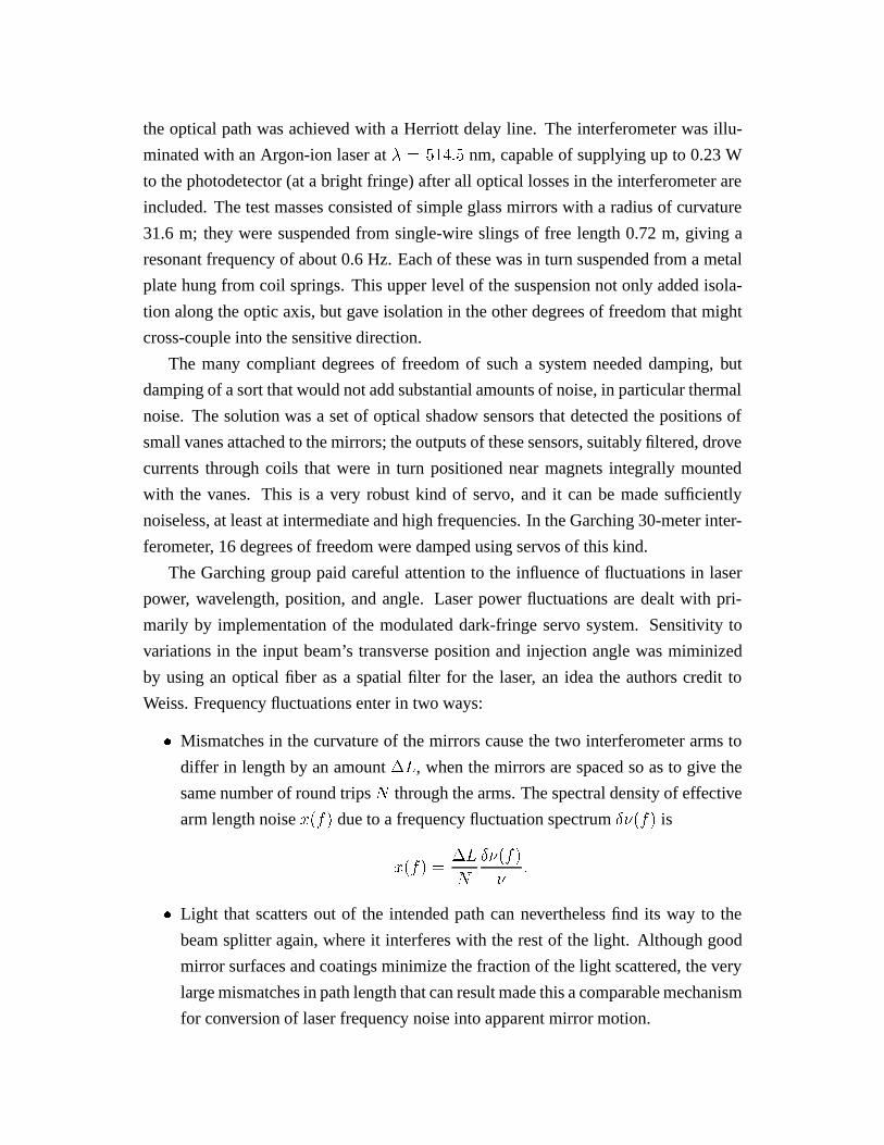
the optical path was achieved with a Herriott delay line. The interferometer was illu-

minated with an Argon-ion laser at� = 514:5 nm, capable of supplying up to 0.23 W

to the photodetector (at a bright fringe) after all optical losses in the interferometer are

included. The test masses consisted of simple glass mirrors with a radius of curvature

31.6 m; they were suspended from single-wire slings of free length 0.72 m, giving a

resonant frequency of about 0.6 Hz. Each of these was in turn suspended from a metal

plate hung from coil springs. This upper level of the suspension not only added isola-

tion along the optic axis, but gave isolation in the other degrees of freedom that might

cross-couple into the sensitive direction.

The many compliant degrees of freedom of such a system needed damping, but

damping of a sort that would not add substantial amounts of noise, in particular thermal

noise. The solution was a set of optical shadow sensors that detected the positions of

small vanes attached to the mirrors; the outputs of these sensors, suitably filtered, drove

currents through coils that were in turn positioned near magnets integrally mounted

with the vanes. This is a very robust kind of servo, and it can be made sufficiently

noiseless, at least at intermediate and high frequencies. In the Garching 30-meter inter-

ferometer, 16 degrees of freedom were damped using servos of this kind.

The Garching group paid careful attention to the influence of fluctuations in laser

power, wavelength, position, and angle. Laser power fluctuations are dealt with pri-

marily by implementation of the modulated dark-fringe servo system. Sensitivity to

variations in the input beam’s transverse position and injection angle was miminized

by using an optical fiber as a spatial filter for the laser, an idea the authors credit to

Weiss. Frequency fluctuations enter in two ways:

� Mismatches in the curvature of the mirrors cause the two interferometer arms to

differ in length by an amount�L, when the mirrors are spaced so as to give the

same number of round tripsN through the arms. The spectral density of effective

arm length noisex(f) due to a frequency fluctuation spectrum��(f) is

x(f) =�L

N

��(f)

�:

� Light that scatters out of the intended path can nevertheless find its way to the

beam splitter again, where it interferes with the rest of the light. Although good

mirror surfaces and coatings minimize the fraction of the light scattered, the very

large mismatches in path length that can result made this a comparable mechanism

for conversion of laser frequency noise into apparent mirror motion.

In order to make laser frequency noise small enough, the Garching group stabilized

the laser using a combination of two servo loops. In the first loop, a rigid Fabry-Perot

resonant cavity serves as a length reference; the light’s wavelength is held to resonance

in the cavity, by inspection of the transmitted light intensity. A second error signal is

derived by interfering the light that exits the bright port of the interferometer (whose

phase depends on the average of the lengths of the two arms) with some of the new light

entering. Feedback was applied to a mirror at the end of the laser cavity, to a Pockels

cell within the laser cavity, and to the common mode positions of the two end mirrors

of the interferometer.

The noise spectrum of the system was in reasonable agreement with a noise budget

prepared from estimates of the noise sources described above. The rms noise in a 1 kHz

bandwidth near 1 kHz was about3� 10�18, only a factor of three poorer than the best

that had been achieved by a resonant-mass detector. This was one of the great triumphs

of the German work. The other was the robustness of the rather elaborate active system

that this interferometer had become, of order two dozen servo loops. It typically stayed

in lock for 30 minutes to an hour, and upon losing lock would shortly reacquire lock

automatically.

The 30-meter interferometer was run for 100 hours in March, 1989, in coincidence

with the 10-meter interferometer at Glasgow that had achieved comparable sensitivity.

Even then, the enthusiasm for looking for gravitational waves at “low” sensitivity was

such that an analysis of the results of the run was not published until 1996.71

6.7 Designs for kilometer-class interferometers

As noted above, laboratory work on interferometers was almost from the beginning

considered an engineering exercise preparatory to the construction of instruments with

arms of kilometer scale. With several such devices now under construction, it is worth

reviewing their distinctive features. Here, even more so than for the other cases we

have been discussing, the refereed literature is a poor source of information, and so

are conference proceedings. For most projects the only detailed descriptions are those

contained in funding proposals. (The one redeeming feature of this form of publication

is that, since the reviewers of such documents were typically not expected to be experts

in the field, they contain an abundance of carefully written tutorial material, and well-

reasoned justifications for most design choices.)

The three largest approved projects today, (LIGO,72 VIRGO,73 and GEO74) all went

through similar parallel processes of design study, proposal, and now construction. This

was a fruitful period, with a rich interchange of ideas. For pedagogical purposes, we

choose to focus in this review on a single line of development, that of the U.S. LIGO

Project.

6.7.1 The “Blue Book”

In almost the same sense as the early table-top interferometers were prototypes of larger

instruments, so too did the proposals for kilometer-scale interferometers have a proto-

type. This was the report called “A Study of a Long Baseline Gravitational Wave An-

tenna System”, submitted to the U.S. National Science Foundation in October 1983.75

(It has since its presentation been called the “Blue Book” because of the color of the

cheap paper cover in which it was bound.) It was prepared primarily by Weiss and two

colleagues at MIT (Paul S. Linsay and the present author), as the product of a plan-

ning exercise funded by the NSF starting in 1981. The report also contained a section

by Stan Whitcomb of Caltech on Fabry-Perot systems (as a partial counter to Weiss’

emphasis on Herriott delay lines), as well as extensive sections written by industrial

consultants from Stone & Webster Engineering Corporation and from Arthur D. Lit-

tle, Inc. These latter contributors were essential, because this document contains, for

the first time anywhere, an extensive discussion of the engineering details specific to

the problems of the construction and siting of a large interferometer. The report was

presented, by both Weiss’ MIT group and that of Drever at Caltech, at a meeting of

the NSF’s Advisory Council for Physics late in 1983. While not a formal proposal, it

served as a sort of “white paper”, suggesting the directions that subsequent proposals

might (and in large measure did) take.

The first half of the report is devoted to the physics of gravitational wave interferom-

eters. This section reads much like Weiss’ 1972 design study, except that many issues

only touched on briefly in the first paper are here discussed at substantially greater

length. In the eleven years that elapsed between the two documents there had been real

progress on several fronts. There are chapters on sources of gravitational waves, the

basic physics of the response of a free-mass interferometer to a gravitational wave, a

discussion of beam-folding schemes and a summary of the current prototype interfer-

ometers, and another extensive discussion of noise sources. The report is bracketed by

an introductory section outlining a history of the field to 1983 and by a pair of appen-

dices, one of which compares the quantum limits of bars and interferometers and the

other showing why the interferometer beams must travel through an evacuated space

instead of through optical fibers.

The main emphasis of the Blue Book was less a discussion of physicsper sethan

it was a consideration of the practical aspects of the experiment as an engineering and

construction project. The completely new material appears in the second half of the

Blue Book, in the chapters summarizing the work of the industrial consultants. Weiss

believed that the only significant impediment to achieving astrophysically interesting

sensitivity was the expense of building an interferometer with long arms (the issue that

had brought the Hughes group’s progress to a halt.) The industrial study was undertaken

with the aim of identifying what design trade-offs would allow for a large system to be

built at minimum cost, and to establish a rough estimate of that cost (along with cost

scaling laws) so that the NSF could consider whether it might be feasible to proceed

with a full-scale project.

Before such an engineering exercise could be meaningful, though, it was necessary

to define what was meant by “full-scale”. The Blue Book approaches this question

by first modeling the total noise budget as a function of frequency, then evaluating

the model as a function of arm lengths ranging from 50 meters (not much longer than

the Caltech prototype) to 50 km. The design space embodied in this model was then

explored in a process guided by three principles:

� “The antenna should not be so small that the fundamental limits of performance

can not be attained with realistic estimates of technical capability.” This was taken

to mean that the length ought to be long enough that one could achieve shot noise

limited performance for laser power of 100 W, without being limited instead by

displacement noise sources, over a band of interesting frequencies. The length

resulting from this criterion strongly depended on whether one took that band to

begin around 1 kHz (in which caseL = 500 m was adequate), 100 Hz (where

L = 5 km was only approaching the required length), or lower still (in which

case evenL = 50 km would not suffice.) Evidently, this strictly physics-based

criterion was too elastic to be definitive.

� “The scale of the system should be large enough so that further improvement of

the performance by a significant factor requires cost increments by a substantial

factor.” In other words, the system should be long enough so that the cost is not

dominated by the length-independent costs of the remote installation.

� “Within reason no choice in external parameters of the present antenna design

should preclude future internal design changes which, with advances in technol-

ogy, will substantially improve performance.” This was a justification for invest-

ing in a large-diameter beam tube, and for making sure that the vacuum system

could achieve pressures as low as10�8 torr.

In an iterative process, rough application of these principles was used to set the

scope of options explored by the industrial consultants. Then at the end of the process,

the principles were used again to select a preferred design. Arm lengths as long as

10 km were explored, and tube diameters as large as 48 inches. An extensive site

survey was also carried out by the consultants. It was aimed at establishing that sites

existed that were suitable for a trenched installation (which put stringent requirements

on flatness of the ground) of a 5 km interferometer. The survey covered Federal land

across the United States, and a study of maps of all land in the Northeastern United

States, along with North Carolina, Colorado, and Nebraska. Thirteen “suitable” sites

were identified. Evaluation criteria also included land use (specifically that the site not

be crossed by roads, railroads, or oil and gas pipelines), earthquake risk, drainage, and

accessibility.

The site survey also attempted to identify possibilities of locating an interferometer

in a subsurface mine, which would give a more stable thermal environment and perhaps

also reduced seismic noise (if it were located deep enough, and if it were inactive.) No

mines were found in the United States with two straight orthogonal tunnels even 2 km

in length.

The conclusion of the exercise was a “proposed design” with the following features:

� Two interferometer installations separated by “continental” distances.

� Interferometer arm length ofL = 5 km.

� Beam tubes of 48 inch diameter made of aluminum (chosen for an expected

cost savings over stainless steel) pumped by a combination of Roots-blowers for

roughing and ion-pumps for achieving and maintaining the high vacuum. A delay

line interferometer would require a diameter of almost the proposed size. Drever’s

beam-interchange scheme for improved narrow-band sensitivity was also listed as

one justification for preferring large tubes, as was the possibility of multiple inter-

ferometers (presumably based on Fabry-Perot cavities) side by side.

� The proposed installation method was to enclose the tube in a 7’ by 12’ cover

constructed of a “multi-plate pipe-arch”, in turn installed 4 feet below grade in a

trench that was subsequently back-filled with soil.

The total estimated cost for such a system was given as $58M.

Note that there were no specific recommendations for the design of the interferom-

eters themselves, beyond the “straw man” used for estimating the noise budget.

The Blue Book was received respectfully by the NSF’s Advisory Committee for

Physics. As a result, the MIT and Caltech research groups were encouraged to com-

bine their forces to develop a complete specific design. Subsequently, both groups

received funding with the eventual goal of a joint proposal for construction of a large

interferometer system.

6.7.2 The LIGO proposal of December 1987

By 1987, substantial progress had been made on lab-scale interferometers by research

groups around the world. And, encouraged by the NSF’s reception of the Blue Book,

more thinking had gone into the best way to construct and exploit large interferome-

ters. Much of this progress is evident in the proposal submitted to the U.S. National

Science Foundation in December of 1987 by a formal Caltech-MIT collaboration that

had adopted the name of LIGO, for Laser Interferometer Gravitational wave Observa-

tory.76 Since September 1987 it had been led by Rochus E. (“Robbie”) Vogt as Project

Director, with Drever and Weiss as science team leaders. The proposal requested funds

for a three-year program of R&D and engineering studies, the outcome of which was

intended to be another proposal (to be submitted in 1989) requesting authorization to

build a pair of 4 km long interferometers.

Prototype interferometers were functioning at respectable sensitivities, after years

of assembly, debugging, analysis, and redesign. The Caltech 40-meter interferome-

ter was the showpiece of the proposal. It employed high-finesse Fabry-Perot cavities,

arranged in the simplified non-recombined configuration for ease of testing. An im-

pressive graph shows the improvement in strain sensitivity since its first operation in

May 1983, by a factor of over103 in amplitude. In that interval, ultra-low loss “su-

permirrors” were installed, first on an early optical-bench style of test mass and then

on separated compact test masses (eventually ones made of fused silica), and a variety

of improvements were made to the Argon laser and to the locking servos. The noise

spectrum above 1 kHz was nearly white, with a level ofh(f) � 2� 10�19=pHz. This

was consistent with the expected level of shot noise.

Results were also presented from the table-top (1.5 meter arm length) prototype

interferometer at MIT. It employed Herriott delay lines of 56 bounces between con-

ventional high quality mirrors that were clamped to aluminum test masses. Unlike the

Caltech instrument which could not function without sophisticated frequency stabiliza-

tion of its laser, MIT used an unstabilized Argon laser to which phase noise was actually

added to help suppress scattered light. Pointing, damping, and slow feedback were ac-

complished with electrostatic actuators. Strain sensitivity could of course not compete

with the much longer Caltech instrument, but even the displacement noise was nearly

an order of magnitude worse, given as4:6 � 10�17 m=pHz, for frequencies above 4

kHz. That level was a factor of 2 in excess of the expected shot noise in the 60 mW of

light, diagnosed as insufficiently suppressed noise from scattered light. At lower fre-

quencies acoustic noise drove the interferometer via a variety of coupling paths through

the injection optics as well as the test mass suspensions.

The proposal records substantial progress toward design of a full-scale interferom-

eter. It states that the collaboration had adopted the Fabry-Perot beam-folding system.

A preliminary design is presented in an appendix of the proposal. It envisioned use

of 5 to 6 W of light at 514 nm from an Argon laser employed in a power recycled

configuration. An elaborate schematic diagram gave a hint of the complexity of the

servos necessary to control the large number degrees of freedom that need to be kept

locked for such an instrument to function. These include lengths of the arm cavities,

the separation of their input mirrors from the beam splitter, the location of the power

recycling mirror, and the lengths of various “mode cleaning” resonant cavities used for

spatial filtering of the laser beam. In addition to these lengths, control of a number of

angular degrees of freedom also needs to be included. Four separate RF modulation

frequencies are specified to drive these servos. Special features are designed into the

main cavity locking servo so that the phase modulation can be injected with a small

Pockels cell without the inevitable losses dominating the performance of the recycling

system.

Another appendix describes an alternate optical configuration based on Herriott de-

lay lines. It employed 86 cm diameter silicon test masses of 450 kg. The simplicity

of the servos was listed as one of its major advantages. A “closed-path” variation of

this design was also presented, in which light leaving one arm is injected into the other.

This is like a single-interchange version of Drever’s system for improving sensitivity to

periodic waves. Here it was employed mainly to relax the tolerances on matching the

curvature of the large mirrors. (The virtues of this design have recently been explored

again by the Stanford group.77)

On the engineering and site issues there had also been some progress since the Blue

Book study, mostly made by engineers at Caltech’s Jet Propulsion Laboratory, but this

was not considered complete enough to highlight in the proposal. Instead, one of the

first proposed tasks was to complete a preliminary engineering design. Nevertheless, a

mature understanding had been achieved of what LIGO ought tobe. This insight was

expressed in a list of “Essential Features of the LIGO”:

1. “Two widely separated sites under common management.” Two sites had been a

feature of Weiss’ earliest thinking, to allow coincidence observations to search for

transient signals. The new feature was the commitment to truly have them man-

aged as a single entity, “to guarantee that two receivers of nearly equal sensitivity

are on line simultaneously at two sites, with a high live time.”

2. “Arm lengths of order 4 kilometers at each site,” a slight scaling back of the 5

km considered previously, but still long enough to strongly dilute the effects of

displacement noise.

3. “The ability to operate simultaneously several receiver systems at each site.” In

a way, this was the most ambitious feature of the LIGO concept. In part it grew

out of a kind of conservatism that was not clearly spelled out, but that was nev-

ertheless real. The early LIGO interferometers, if they were not to be extremely

risky extrapolations from known technology, were unlikely to have sufficient sen-

sitivity to be assured of detecting astrophysical signals. Even if that weren’t so,

the project would have had to wrestle with the competition between time devoted

to observation and time devoted to improving the performance of the instrument.

This competition had bedeviled workers on resonant-mass detectors. The key new

idea for LIGO was that the precious commodity, an evacuated beam pipe, might

be available with abundant cross-sectional area since the Fabry-Perot geometry

had been adopted. All that was required was an arrangement of tanks at the ends

of the pipe to install the test masses of various interferometers, both operational

and experimental. This actually called for substantial cleverness in developing an

airlock system, so that installation and operation could take place with “a mini-

mum of mutual interference”.

4. “The capability for receivers of two different arm lengths.” Drever urged the adop-

tion of this feature, to allow a clean test of the gravitational origin of candidate

signals, which should show up as the tidal signature that a longer interferometer

sees twice the signal.

5. “A vacuum tube diameter of order 48 inches.” This had the conservative justifica-

tion that it would be necessary if one had to switch from Fabry-Perot cavities to

delay lines, and the great benefit of allowing multiple Fabry-Perot interferometers,

as mentioned above.

6. “The capability of a vacuum level of10�8 torr.” This would be needed, not for the

first LIGO instrument, but to avoid having fluctuations in the index of refraction

of the residual gas dominate shot noise in a more sensitive “advanced” receiver.

7. “A minimum lifetime of the facilities of 20 years.” This was to be not just a

one-shot discovery experiment, but a laboratory to exploit the gravitational wave

window in astronomy.

8. “Adequate support instrumentation.”

The heritage of the Blue Book should be evident in the above list, but so too should

be the progress in thinking beyond that point.

Because of a Federal budget crisis, this proposal was not funded. However, the

two groups were encouraged to continue their work, and to submit a more complete

proposal in a subsequent year.

6.7.3 The LIGO proposal of December 1989

Many of the features only hinted out in the 1987 proposal are spelled out in much

greater detail in the proposal for engineering design and construction of LIGO (now

with a hyphen in Laser Interferometer Gravitational-Wave Observatory) that was sub-

mitted to the NSF in December 1989.78 It fleshes out the design of a system that would

embody the eight Essential Features of LIGO first described in the 1987 proposal. (The

only differences are that the vacuum tube diameter is now specified as a “clear optical

diameter of approximately 1 meter”, and the vacuum spec is given as “10�9 torr of

hydrogen and10�10 of other gases.”)

A single detector system would require three interferometers — a 4 km interferom-

eter at each of two widely separated remote sites, plus a 2 km interferometer at one of

the sites. This shorter interferometer played two related roles: a check that a candi-

date signal had the tidal signature of a gravitational wave, and the simpler but crucial

requirement that a real signal should appear in all three interferometers. A calculation

presented here shows that an accidental event rate of around 100/hour/interferometer

can be tolerated without accidental 3-way coincidences occurring more frequently than

once in ten years, an improvement of about two orders of magnitude over what could

be tolerated with only a single interferometer at each site.

The features described above are part of a plan that is aimed at accomplishing “three

primary objectives”:

� “observation”, or a continuous “gravitational-wave watch”,

� “development”, or “full functional testing of new and advanced interferometer-

based detector concepts”, and

� “special investigations” using detectors optimized for “particular phenomena”.

These missions are “to be conducted without mutual interference.”

It would take a substantial investment (of money, ideas, and energy of scientists) to

accomplish all of these goals, and so for this reason full implementation of this strategy

was to be accomplished in a series of phases.

� “Phase A, The Exploration/Discovery Phase”, with one three-interferometer de-

tector system, suitable for observation or development, but not both simultane-

ously.

� “Phase B, The Discovery/Observation Phase”, with two three-interferometer de-

tector systems, allowing “concurrent observationanddevelopment or specialized

search.”

� “Phase C, The Observatory Phase”, room for three full detector systems, “allows

concurrent observation, development, special investigations, and optimal access

for the scientific community at large. It completes the LIGO evolution to its

presently conceived full-design capability.”

Because of the cost involved in elaborate vacuum chambers with airlocks, the 1989

proposal asked only for the funds to complete Phase A. The single important investment

in the capability to upgrade to Phases B and C was the design of buildings large enough

to accomodate all of the vacuum tanks that would be eventually required.

It should be emphasized that, to a large degree, this agressive planning for an elab-

orate facility was a necessary consequence of a simple fact — that it looked difficult

to build an interferometer that would have sufficient sensitivity to assure detection of

gravitational waves. Hence the need to plan for ongoing interferometer development

and specially optimized instruments. Of course, these activities would also be useful

even if some signals proved easier to detect than expected, since carrying out gravita-

tional wave astronomy would call for the highest achievable signal to noise ratios. For

example, angular position errors are inversely proportional to the signal to noise ratio,

and are as large as 10 arcmin or more when the SNR= 10, even when observations are

made with a three-detector U.S.-Europe network.

The 1989 proposal is much more explicit about the details of the design of the first

interferometer. The design is based on the Fabry-Perot interferometer of the 1987 pro-

posal’s appendix. It has been fleshed out with specifications of laser power, finesse,

test mass parameters and vibration isolation performance, so that a specific noise bud-

get could be presented. The 1989 proposal also contains a preliminary discussion of

what sorts of improvements would be necessary to push the noise to levels low enough

to guarantee detection of signals. This includes laser power of 60 W recycled by a

factor of 100, a much more aggressive vibration isolation system, and final pendulum

suspensions with a quality factor of109 carrying 1-ton fused silica mirrors.

6.7.4 The situation today

Construction of LIGO was approved in 1991. By mid-1998 (the time of the writing of

this review), construction of the two facilities in Hanford WA and Livingston LA was

over three-quarters complete. The schedule calls for construction to be completed soon.

Roughly speaking, 1999 is to be devoted to installation of the scientific equipment in the

completed facilities, 2000 to shakedown of the interferometers, and 2001 to engineering

activities to bring the performance up to the design specifications. Then, data will be

collected during 2002-3. Beginning in 2004, upgrades to improve the performance will

be carried out, interspersed with additional periods of observation.

The first instrument to be installed is expected to have a noise spectrum like that

shown in Figure 4. The high frequency noise spectrum should be dominated by shot

noise, as determined from an input power of 6 W, multiplied by a power recycling gain

of 30. Thermal noise from the 1 Hz pendulum mode will dominate the intermediate

frequency band; the oscillations of the 10 kg test masses should achieve a quality factor

of 1:6� 105. (Internal thermal noise will dominate the spectrum only in a narrow band,

due to test mass modal quality factors of about106.) Low frequency noise will be

governed of course by seismic noise that passes through the multi-layer stack.

Performance of the VIRGO 3 km interferometer will be similar at medium and high

frequencies. At low frequencies, seismic noise should be much lower in VIRGO than

in LIGO, since a much more aggresive filter has been designed. This should allow the

noise to be dominated by pendulum thermal noise down to 10 Hz or a bit lower.

The GEO 600 meter interferometer is not expected to reach quite such low levels,

100

101

102

103

104

10−25

10−24

10−23

10−22

10−21

10−20

10−19

10−18

10−17

10−16

Frequency (Hz)

h(f)

(1/

sqrt

(Hz)

)

seismic

shotpendulum thermal

internal thermal

Fig. 4. An estimate of the noise spectrum of the LIGO I interferometers. The four

most important noise sources are shown: seismic noise, pendulum mode thermal noise,

thermal noise of internal vibrations of the mirror, and shot noise.

but it will be surprisingly close. To make up for the shorter length, advanced technolo-

gies (including signal recycling) will be pursued aggressively from an early date. Thus

this instrument will play a dual role as part of the global network of interferometers and

as a prototype for features that will later be incorporated into other interferometers.

References

[1] E. M. Purcell,Electricity and Magnetism, (McGraw-Hill, New York, 1965).

[2] L. D. Landau and E. M. Lifschitz,The Classical Theory of Fields, (Pergamon,

Oxford, 1975).

[3] P. Kafka, inSpace Science and Fundamental Physics, Proceedings of Summer

School, Alpbach, Austria, 28 July - 7 August 1987 (ESA SP-283, May 1988).

[4] A. P. Cowley,Ann. Rev. Astron. Astrophys.30, 287 (1992).

[5] J. A. Wheeler, cited in Weber (1961).

[6] J. Weber,Phys. Rev.117, 306 (1960).

[7] J. Weber,General Relativity and Gravitational Waves(Interscience, New York,

1961).

[8] J. Weber,Phys. Rev. Lett.22, 1320 (1969).

[9] F. A. E. PiraniActa. Phys. Polon.15, 389 (1956).

[10] G. E. Moss, L. R. Miller, and R. L. Forward,Appl. Opt.10, 2495 (1971).

[11] R. Weiss,Quarterly Progress Report, MIT Research Lab of Electronics105, 54

(1972).

[12] E. Kappler,Ann. Phys. (Leipzig)11, 233 (1931); R. B. Barnes and S. Silverman,

Rev. Mod. Phys.6, 162 (1934).

[13] J. B. Johnson,Phys. Rev.32, 97 (1928).

[14] H. Nyquist,Phys. Rev.32, 110 (1928).

[15] H. B. Callen and T. A. Welton,Phys. Rev.83, 34 (1951); H. B. Callen and R. F.

Greene,Phys. Rev.86, 702 (1952).

[16] N. Bohr,Nature121, 580 (1928).

[17] N. Bohr, in Albert Einstein: Philosopher-Scientist(Library of Living Philoso-

phers, Evanston, Ill., 1949).

[18] R. Weiss, inSources of Gravitational Radiation, ed. L. Smarr (Cambridge Uni-

versity Press, Cambridge, 1979) p. 7.

[19] P. A. M. Dirac,The Principles of Quantum Mechanics(Clarendon Press, Oxford,

1958).

[20] C. M. Caves,Phys. Rev. Lett.45, 75 (1980).

[21] J. Weber,Phys. Rev. Lett.17, 1228 (1966).

[22] R. Del Fabbro, A. diVirgilio, A. Giazotto, H. Kautzky, V. Montelatici, and D.

Passuello,Phys. Lett. A132, 237 (1988).

[23] J. L. Levine and R. L. Garwin,Phys. Rev. Lett.31, 173 (1973).

[24] E. Amaldi O. Aguiar, M. Bassan, P. Bonifazi, P. Carelli, M. G. Castellano, G.

Cavallari, E. Coccia, C. Cosmelli, W. M. Fairbank, S. Frasca, V. Foglietti, R.

Habel, W. O. Hamilton, J. Henderson, W. Johnson, K. R. Lane, A. G. Mann, M.

S. McAshan, P. F. Michelson, I. Modena, G. V. Pallottino, G. Pizzella, J. C. Price,

R. Rapagnani, F. Ricci, N. Solomonson, T. R. Stevenson, R. C. Taber, and B.-X.

Xu, Astron. Astrophys.216, 325 (1989).

[25] G. W. Gibbons and S. W. Hawking,Phys. Rev. D4, 2191 (1971).

[26] H. J. Paik,J. Appl. Phys.47, 1168 (1976).

[27] J. P. Richard and W. M. Folkner, inThe Detection of Gravitational Waves, ed. D.

G. Blair, (Cambridge University Press, Cambridge, 1991).

[28] V. B. Braginsky and Yu. I. Vorontsov,Sov. Phys. Uspekhi17, 644 (1974).

[29] M. E. Tobar and D. G. Blair,J. Phys. D: Appl. Phys.26, 2276 (1993).

[30] P. R. Saulson,Class. Quantum Grav.14 , 2435 (1997).

[31] H. Rothe and W. Dahlke,Proc. IRE44, 811 (1956).

[32] W. R. LePage,Complex Variables and the Laplace Transform for Engineers

(McGraw-Hill, New York, 1961).

[33] J.-P. Richard,Phys. Rev. Lett.52, 165 (1984); J. C. Price,Phys. Rev. D36, 3555

(1987).

[34] R. W. P. Drever, J. Hough, R. Bland, and G. W. Lessnoff,Nature246, 340 (1973).

[35] H. Heffner,Proc. IRE50, 1604 (1962).

[36] R. P. Giffard,Phys. Rev. D14, 2478 (1976).

[37] J. Weber,Phys. Rev. Lett.24, 276 (1970).

[38] J. Weber,Phys. Rev. Lett.25, 180 (1970).

[39] W. H. Press and K. S. Thorne,Ann. Rev. Astron. Astrophys.10, 334 (1972).

[40] P. S. Aplin,Gen. Rel. Grav.3, 111 (1972).

[41] J. Weber, V. Hughes, P. Kafka, R. W. P. Drever, and C. W. MisnerAnn. N.Y. Acad.

Sci.224, 101 (1973).

[42] D. Bramanti and K. Maischberger,Lett. Nuovo Cimento4 , 1007 (1972); D. Bra-

manti, K. Maischberger, and D. Parkinson,Lett. Nuovo Cimento7, 665 (1973).

[43] H. Billing, P. Kafka, K. Maischberger, F. Meyer, and W. Winkler,Lett. Nuovo

Cimento12, 111 (1975).

[44] J. A. Tyson,Ann. N.Y. Acad. Sci.224, 74 (1973).

[45] J. L. Levine and R. L. Garwin,Phys. Rev. Lett.31, 173 (1973); R. L. Garwin and

J. L. Levine,Phys. Rev. Lett.31, 176 (1973); J. L. Levine and R. L. Garwin,Phys.

Rev. Lett.33, 794 (1974).

[46] J. L. Levine and R. L. Garwin (1974), cited above.

[47] R. L. Garwin,Physics Today, December 1974, p. 9.

[48] D. Sciama, J. Weber, P. Kafka, R. W. P. Drever, J. A. Tyson, inGeneral Relativity

and Gravitation, Proceedings of GR7, Tel Aviv University, June 23-28, 1974, eds.

G. Shaviv and J. Rosen (Wiley, New York 1974).

[49] H. M. Collins,Changing Order(Sage Publications, London, 1985). See also this

exchange: A. Franklin,Stud. Hist. Phil. Sci.25, 463 (1994); H. M. Collins,Stud.

Hist. Phil. Sci.25, 493 (1994).

[50] R. W. P. Drever,Q. Jl. R. astr. Soc.18, 9 (1977).

[51] J. A. Tyson and R. P. Giffard,Ann. Rev. Astron. Astrophys.16, 521 (1978).

[52] P. Kafka and L. Schnupp,Astron. Astrophys.70, 97 (1978).

[53] S. P. Boughn, W. M. Fairbank, R. P. Giffard, J. N. Hollenhorst, E. R. Mapoles, M.

S. McAshan, P. F. Michelson, H. J. Paik, and R. C. Taber,Ap. J. Lett.261, L19

(1982).

[54] P. Astoneet al., Proceedings of the Xth Italian General Relativity Conference,

Bardonecchia, September 1-4, 1992, unpublished.

[55] M. Aglietta, A. Castellina, W. Fulgione, G. Trinchero, S. Vernetto, P. Astone,

G. Badino, G. Bologna, M. Bassan, E. Coccia, I. Modena, P. Bonifazi, M. G.

Castellano, M. Visco, C. Castagnoli, P. Galeotti, O. Saavedra, C. Cosmelli, S.

Frasca, G. V. Pallottino, G. Pizzella, P. Rapagnani, F. Ricci, E. Majorana, D. Gretz,

J. Weber, and G. Wilmot,Nuovo Cimento106B, 1257 (1991); G. Pizzella, in

Develpments in General Relativity, Astrophysics and Quantum Theory: A Jubilee

in Honour of Nathan Rosen, eds. F. Cooperstock, L. P. Horwitz, and J. Rosen,

Annals of the Israel Physical Society9, 195 (1990).

[56] C. A. Dickson and B. F. Schutz,Phys. Rev. D51, 2644 (1995).

[57] M. E. Gertsenshtein and V. I. Pustovoit,Sov. Phys. JETP16, 433 (1962).

[58] P. G. Roll, R. Krotkov, and R. H. Dicke,Ann. Phys. (N.Y.)26, 442 (1964).

[59] A. A. Michelson and E. W. Morley,Am. J. Sci.34, 333 (1887).

[60] R. H. Dicke,Rev. Sci. Instrum.17, 268 (1946).

[61] R. Buderi,The Invention That Changed the World(Simon and Schuster, New

York, 1996).

[62] J. D. Kraus,Radio Astronomy(McGraw-Hill, New York, 1966).

[63] R. H. Dicke,The Theoretical Significance of Experimental Relativity(Gordon and

Breach, New York, 1964).

[64] R. L. Forward,Phys. Rev. D17, 379 (1978).

[65] R. W. P. Drever, inGravitational Radiation, eds. N. Deruelle and T. Piran (North

Holland, Amsterdam, 1983), p. 321.

[66] R. W. Drever, J. L. Hall, F. V. Kowalski, J. Hough, G. M. Ford, A. J. Munley, and

H. Ward,Appl. Phys. B31, 97 (1983); see also A. Schenzle, R. DeVoe, and G.

Brewer,Phys. Rev. A25, 2606 (1982).

[67] R. V. Pound,Rev. Sci. Instrum.17, 490 (1946).

[68] B. J. Meers,Phys. Rev. D38, 2317 (1988); K. A. Strain and B. J. Meers,Phys.

Rev. Lett.66, 1391 (1991).

[69] D. Shoemaker, R. Schilling, L. Schnupp, W. Winkler, K. Maischberger, and A.

Rudiger,Phys. Rev. D38, 423 (1988).

[70] P. F. Michelson, Hu E.-K., and G. Pizzella, eds.,International Symposium on

Experimental Gravitational Physics(World Scientific, Singapore, 1988).

[71] D. Nicholson, C. A. Dickson, W. J. Watkins, B. F. Schutz, J. Shuttleworth, G. S.

Jones, D. I. Robertson, N. L Mackenzie, K. A. Strain, B. J. Meers, G. P. New-

ton, H. Ward, C. A. Cantley, N. A. Robertson, J. Hough, K. Danzmann, T. M.

Niebauer, A. R¨udiger, R. Schilling, L. Schnupp, and W. Winkler,Phys. Lett. A

218, 175 (1996).

[72] A. Abramovici, W. E. Althouse, R. W. P. Drever, Y. G¨ursel, S. Kawamura, F. J.

Raab, D. Shoemaker, L. Sievers, R. E. Spero, K. S. Thorne, R. E. Vogt, R. Weiss,

S. E. Whitcomb, and M. E. Zucker,Science256, 325 (1992).

[73] C. Bradaschia, R. Del Fabbro, A. Di Virgilio, A. Giazotto, H. Kautzky, V. Mon-

telatici, D. Passuello, A. Brillet, O. Cregut, P. Hello, C. N. Man, P. T. Manh, A.

Marraud, D. Shoemaker, J.-Y. Vinet, F. Barone, L. Di Fiore, L. Milano, G. Russo,

S. Solimeno, J. M. Aguirregabiria, H. Bel, J.-P. Duruisseau, G. Le Denmat, P.

Tourrenc, M. Capozzi, M. Longo, M. Lops, I. Pinto, G. Rotoli, T. Damour, S.

Bonazzola, J. A. Marck, Y. Gourghoulon, L. E. Holloway, F. Fuligni, V. Iafolla,

G. Natale,Nucl. Instr. Meth. Phys. Res. A289, 518 (1990).

[74] J. Hough, G. P. Newton, N. A. Robertson, H. Ward, A. M. Campbell, J. E. Logan,

D. I. Robertson, K. A. Strain, K. Danzmann, H. L¨uck, A. Rudiger, R. Schilling,

M. Schrempel, W. Winkler, J. R. J. Bennett, V. Kose, M. K¨uhne, B. F. Schutz, D.

Nicholson, J. Shuttleworth, H. Welling, P. Aufmuth, R. Rinkleff, A. T¨unnermann,

and B. Willke, inProceedings of the Seventh Marcel Grossmann Meeting on Gen-

eral Relativity, eds. R. T. Jantzen and G. M. Keiser (World Scientific, Singapore,

1996), p. 1352.

[75] P. S. Linsay, P. R. Saulson, and R. Weiss,A Study of a Long Baseline Gravitational

Wave Antenna System(MIT, Cambridge, Mass., 1983), unpublished.

[76] R. E. Vogt, R. W. P. Drever, K. S. Thorne, and R. Weiss,Caltech/MIT Project for

a Laser Interferometer Gravitational Wave Observatory, proposal to the National

Science Foundation (Caltech, Pasadena, 1987), unpublished.

[77] K.-X. Sun, M. M. Fejer, E. Gustafson, and R. L. Byer,Phys. Rev. Lett.76, 3053

(1996).

[78] R. E. Vogt, R. W. P. Drever, F. J. Raab, K. S. Thorne, and R. Weiss,The Con-

struction, Operation, and Supporting Research and Development of a Laser In-

terferometer Gravitational-Wave Observatory, proposal to the National Science

Foundation (Caltech, Pasadena, 1989), unpublished.