Calibration of the LIGO Gravitational Wave Detectors

in the Fifth Science Run

J. Abadie19, B. P. Abbott19, R. Abbott19, M, Abernathy51, C. Adams21,R. Adhikari19, P. Ajith19, B. Allen2,78, G. Allen37, E. Amador Ceron63,

R. S. Amin23, S. B. Anderson19, W. G. Anderson63, M. A. Arain50,M. Araya19, M. Aronsson19, Y. Aso19, S. Aston49, D. E. Atkinson20,

P. Aufmuth18, C. Aulbert2, S. Babak1, P. Baker26, S. Ballmer19,D. Barker20, S. Barnum34, B. Barr51, P. Barriga62, L. Barsotti22,

M. A. Barton20, I. Bartos11, R. Bassiri51, M. Bastarrika51, J. Bauchrowitz2,B. Behnke1, M. Benacquista44, A. Bertolini2, J. Betzwieser19,

N. Beveridge51, P. T. Beyersdorf33, I. A. Bilenko27, G. Billingsley19,J. Birch21, R. Biswas63, E. Black19, J. K. Blackburn19, L. Blackburn22,

D. Blair62, B. Bland20, O. Bock2, T. P. Bodiya22, R. Bondarescu39,R. Bork19, M. Born2, S. Bose64, M. Boyle7, P. R. Brady63,

V. B. Braginsky27, J. E. Brau56, J. Breyer2, D. O. Bridges21,M. Brinkmann2, M. Britzger2, A. F. Brooks19, D. A. Brown38,

A. Buonanno52, J. Burguet–Castell63, O. Burmeister2, R. L. Byer37,L. Cadonati53, J. B. Camp28, P. Campsie51, J. Cannizzo28, K. C. Cannon19,

J. Cao46, C. Capano38, S. Caride54, S. Caudill23, M. Cavaglia41,C. Cepeda19, T. Chalermsongsak19, E. Chalkley51, P. Charlton10,

S. Chelkowski49, Y. Chen7, N. Christensen9, S. S. Y. Chua4,C. T. Y. Chung40, D. Clark37, J. Clark8, J. H. Clayton63, R. Conte58,D. Cook20, T. R. Corbitt22, N. Cornish26, C. A. Costa23, D. Coward62,

D. C. Coyne19, J. D. E. Creighton63, T. D. Creighton44, A. M. Cruise49,R. M. Culter49, A. Cumming51, L. Cunningham51, K. Dahl2,

S. L. Danilishin27, R. Dannenberg19, K. Danzmann2,28, K. Das50,B. Daudert19, G. Davies8, A. Davis13, E. J. Daw42, T. Dayanga64,

D. DeBra37, J. Degallaix2, V. Dergachev19, R. DeRosa23, R. DeSalvo19,P. Devanka8, S. Dhurandhar17, I. Di Palma2, M. Dıaz44, F. Donovan22,

K. L. Dooley50, E. E. Doomes36, S. Dorsher55, E. S. D. Douglas20,R. W. P. Drever5, J. C. Driggers19, J. Dueck2, J.-C. Dumas62, T. Eberle2,M. Edgar51, M. Edwards8, A. Effler23, P. Ehrens19, R. Engel19, T. Etzel19,M. Evans22, T. Evans21, S. Fairhurst8, Y. Fan62, B. F. Farr30, D. Fazi30,H. Fehrmann2, D. Feldbaum50, L. S. Finn39, M. Flanigan20, K. Flasch63,S. Foley22, C. Forrest57, E. Forsi21, N. Fotopoulos63, M. Frede2, M. Frei43,

Z. Frei14, A. Freise49, R. Frey56, T. T. Fricke23, D. Friedrich2, P. Fritschel22,

Preprint submitted to Nuclear Physics B July 23, 2010

arX

iv:1

007.

3973

v1 [

gr-q

c] 2

2 Ju

l 201

0

V. V. Frolov21, P. Fulda49, M. Fyffe21, J. A. Garofoli38, I. Gholami1,S. Ghosh64, J. A. Giaime34,31, S. Giampanis2, K. D. Giardina21, C. Gill51,

E. Goetz54, L. M. Goggin63, G. Gonzalez23, M. L. Gorodetsky27, S. Goßler2,C. Graef2, A. Grant51, S. Gras62, C. Gray20, R. J. S. Greenhalgh32,

A. M. Gretarsson13, R. Grosso44, H. Grote2, S. Grunewald1,E. K. Gustafson19, R. Gustafson54, B. Hage18, P. Hall8, J. M. Hallam49,

D. Hammer63, G. Hammond51, J. Hanks20, C. Hanna19, J. Hanson21,J. Harms55, G. M. Harry22, I. W. Harry8, E. D. Harstad56, K. Haughian51,K. Hayama29, J. Heefner19, I. S. Heng51, A. Heptonstall19, M. Hewitson2,

S. Hild51, E. Hirose38, D. Hoak53, K. A. Hodge19, K. Holt21, D. J. Hosken48,J. Hough51, E. Howell62, D. Hoyland49, B. Hughey22, S. Husa47,

S. H. Huttner51, T. Huynh–Dinh21, D. R. Ingram20, R. Inta4, T. Isogai9,A. Ivanov19, W. W. Johnson23, D. I. Jones60, G. Jones8, R. Jones51, L. Ju62,

P. Kalmus19, V. Kalogera30, S. Kandhasamy55, J. Kanner52,E. Katsavounidis22, K. Kawabe20, S. Kawamura29, F. Kawazoe2, W. Kells19,

D. G. Keppel19, A. Khalaidovski2, F. Y. Khalili27, E. A. Khazanov16,H. Kim2, P. J. King19, D. L. Kinzel21, J. S. Kissel23,∗, S. Klimenko50,

V. Kondrashov19, R. Kopparapu39, S. Koranda63, D. Kozak19, T. Krause43,V. Kringel2, S. Krishnamurthy30, B. Krishnan1, G. Kuehn2, J. Kullman2,R. Kumar51, P. Kwee18, M. Landry20, M. Lang39, B. Lantz37, N. Lastzka2,

A. Lazzarini19, P. Leaci2, J. Leong2, I. Leonor56, J. Li44, H. Lin50,P. E. Lindquist19, N. A. Lockerbie61, D. Lodhia49, M. Lormand21, P. Lu37,

J. Luan7, M. Lubinski20, A. Lucianetti50, H. Luck2,28, A. Lundgren38,B. Machenschalk2, M. MacInnis22, M. Mageswaran19, K. Mailand19,

C. Mak19, I. Mandel30, V. Mandic55, S. Marka11, Z. Marka11, E. Maros19,I. W. Martin51, R. M. Martin50, J. N. Marx19, K. Mason22, F. Matichard22,

L. Matone11, R. A. Matzner43, N. Mavalvala22, R. McCarthy20,D. E. McClelland4, S. C. McGuire36, G. McIntyre19, G. McIvor43,

D. J. A. McKechan8, G. Meadors54, M. Mehmet2, T. Meier18, A. Melatos40,A. C. Melissinos57, G. Mendell20, D. F. Menendez39, R. A. Mercer63,L. Merill62, S. Meshkov19, C. Messenger2, M. S. Meyer21, H. Miao62,

J. Miller51, Y. Mino7, S. Mitra19, V. P. Mitrofanov27, G. Mitselmakher50,R. Mittleman22, B. Moe63, S. D. Mohanty44, S. R. P. Mohapatra53,D. Moraru20, G. Moreno20, T. Morioka29, K. Mors2, K. Mossavi2,

C. MowLowry4, G. Mueller50, S. Mukherjee44, A. Mullavey4,H. Muller-Ebhardt2, J. Munch48, P. G. Murray51, T. Nash19, R. Nawrodt51,

J. Nelson51, G. Newton51, A. Nishizawa29, D. Nolting21, E. Ochsner52,J. O’Dell32, G. H. Ogin19, R. G. Oldenburg63, B. O’Reilly21,

2

R. O’Shaughnessy39, C. Osthelder19, D. J. Ottaway48, R. S. Ottens50,H. Overmier21, B. J. Owen39, A. Page49, Y. Pan52, C. Pankow50,

M. A. Papa1,78, M. Pareja2, P. Patel19, M. Pedraza19, L. Pekowsky38,S. Penn15, C. Peralta1, A. Perreca49, M. Pickenpack2, I. M. Pinto59,

M. Pitkin51, H. J. Pletsch2, M. V. Plissi51, F. Postiglione58, V. Predoi8,L. R. Price63, M. Prijatelj2, M. Principe59, R. Prix2, L. Prokhorov27,O. Puncken2, V. Quetschke44, F. J. Raab20, T. Radke1, H. Radkins20,

P. Raffai14, M. Rakhmanov44, B. Rankins41, V. Raymond30, C. M. Reed20,T. Reed24, S. Reid51, D. H. Reitze50, R. Riesen21, K. Riles54, P. Roberts3,

N. A. Robertson29,66, C. Robinson8, E. L. Robinson1, S. Roddy21,C. Rover2, J. Rollins11, J. D. Romano44, J. H. Romie21, S. Rowan51,

A. Rudiger2, K. Ryan20, S. Sakata29, M. Sakosky20, F. Salemi2,L. Sammut40, L. Sancho de la Jordana47, V. Sandberg20, V. Sannibale19,

L. Santamarıa1, G. Santostasi25, S. Saraf34, B. S. Sathyaprakash8, S. Sato29,M. Satterthwaite4, P. R. Saulson38, R. Savage20, R. Schilling2, R. Schnabel2,

R. Schofield56, B. Schulz2, B. F. Schutz1,9, P. Schwinberg20, J. Scott51,S. M. Scott4, A. C. Searle19, F. Seifert19, D. Sellers21, A. S. Sengupta19,

A. Sergeev16, D. Shaddock4, B. Shapiro22, P. Shawhan52,D. H. Shoemaker22, A. Sibley21, X. Siemens63, D. Sigg20, A. Singer19,

A. M. Sintes47, G. Skelton63, B. J. J. Slagmolen4, J. Slutsky23, J. R. Smith6,M. R. Smith19, N. D. Smith22, K. Somiya7, B. Sorazu51, F. C. Speirits51,

A. J. Stein22, L. C. Stein22, S. Steinlechner2, S. Steplewski64, A. Stochino19,R. Stone44, K. A. Strain51, S. Strigin27, A. Stroeer28, A. L. Stuver21,

T. Z. Summerscales3, M. Sung23, S. Susmithan62, P. J. Sutton8,D. Talukder64, D. B. Tanner50, S. P. Tarabrin27, J. R. Taylor2, R. Taylor19,P. Thomas20, K. A. Thorne21, K. S. Thorne7, E. Thrane55, A. Thuring18,

C. Titsler39, K. V. Tokmakov66,76, C. Torres21, C. I. Torrie29,66, G. Traylor21,M. Trias47, K. Tseng37, D. Ugolini45, K. Urbanek37, H. Vahlbruch18,

B. Vaishnav44, M. Vallisneri7, C. Van Den Broeck8, M. V. van der Sluys30,A. A. van Veggel51, S. Vass19, R. Vaulin63, A. Vecchio49, J. Veitch8,

P. J. Veitch48, C. Veltkamp2, A. Villar19, C. Vorvick20, S. P. Vyachanin27,S. J. Waldman22, L. Wallace19, A. Wanner2, R. L. Ward19, P. Wei38,

M. Weinert2, A. J. Weinstein19, R. Weiss22, L. Wen8,77, S. Wen23,P. Wessels2, M. West38, T. Westphal2, K. Wette4, J. T. Whelan31,S. E. Whitcomb19, D. J. White42, B. F. Whiting50, C. Wilkinson20,

P. A. Willems19, L. Williams50, B. Willke2,28, L. Winkelmann2,W. Winkler2, C. C. Wipf22, A. G. Wiseman63, G. Woan51, R. Wooley21,

J. Worden20, I. Yakushin21, H. Yamamoto19, K. Yamamoto2,

3

D. Yeaton-Massey19, S. Yoshida35, P. P. Yu63, M. Zanolin13, L. Zhang19,Z. Zhang62, C. Zhao62, N. Zotov24, M. E. Zucker22, J. Zweizig19

∗ Corresponding Author. 202 Nicholson Hall, Dept. of Physics & Astronomy, LouisianaState University, Tower Dr. Baton Rouge 70803. US Tel.: +1-225-578-0321, Email

address: jkisse1@tigers.lsu.edu.

1Albert-Einstein-Institut, Max-Planck-Institut fur Gravitationsphysik, D-14476 Golm,Germany

2Albert-Einstein-Institut, Max-Planck-Institut fur Gravitationsphysik, D-30167Hannover, Germany

3Andrews University, Berrien Springs, MI 49104 USA

4Australian National University, Canberra, 0200, Australia

5California Institute of Technology, Pasadena, CA 91125, USA

6California State University Fullerton, Fullerton CA 92831 USA

7Caltech-CaRT, Pasadena, CA 91125, USA

8Cardiff University, Cardiff, CF24 3AA, United Kingdom

9Carleton College, Northfield, MN 55057, USA

10Charles Sturt University, Wagga Wagga, NSW 2678, Australia

11Columbia University, New York, NY 10027, USA

13Embry-Riddle Aeronautical University, Prescott, AZ 86301 USA

14Eotvos University, ELTE 1053 Budapest, Hungary

15Hobart and William Smith Colleges, Geneva, NY 14456, USA

16Institute of Applied Physics, Nizhny Novgorod, 603950, Russia

17Inter-University Centre for Astronomy and Astrophysics, Pune - 411007, India

18Leibniz Universitat Hannover, D-30167 Hannover, Germany

19LIGO - California Institute of Technology, Pasadena, CA 91125, USA

20LIGO - Hanford Observatory, Richland, WA 99352, USA

21LIGO - Livingston Observatory, Livingston, LA 70754, USA

22LIGO - Massachusetts Institute of Technology, Cambridge, MA 02139, USA

23Louisiana State University, Baton Rouge, LA 70803, USA

24Louisiana Tech University, Ruston, LA 71272, USA

25McNeese State University, Lake Charles, LA 70609 USA

26Montana State University, Bozeman, MT 59717, USA

4

27Moscow State University, Moscow, 119992, Russia

28NASA/Goddard Space Flight Center, Greenbelt, MD 20771, USA

29National Astronomical Observatory of Japan, Tokyo 181-8588, Japan

30Northwestern University, Evanston, IL 60208, USA

31Rochester Institute of Technology, Rochester, NY 14623, USA

32Rutherford Appleton Laboratory, HSIC, Chilton, Didcot, Oxon OX11 0QX UnitedKingdom

33San Jose State University, San Jose, CA 95192, USA

34Sonoma State University, Rohnert Park, CA 94928, USA

35Southeastern Louisiana University, Hammond, LA 70402, USA

36Southern University and A&M College, Baton Rouge, LA 70813, USA

37Stanford University, Stanford, CA 94305, USA

38Syracuse University, Syracuse, NY 13244, USA

39The Pennsylvania State University, University Park, PA 16802, USA

40The University of Melbourne, Parkville VIC 3010, Australia

41The University of Mississippi, University, MS 38677, USA

42The University of Sheffield, Sheffield S10 2TN, United Kingdom

43The University of Texas at Austin, Austin, TX 78712, USA

44The University of Texas at Brownsville and Texas Southmost College, Brownsville, TX78520, USA

45Trinity University, San Antonio, TX 78212, USA

46Tsinghua University, Beijing 100084 China

47Universitat de les Illes Balears, E-07122 Palma de Mallorca, Spain

48University of Adelaide, Adelaide, SA 5005, Australia

49University of Birmingham, Birmingham, B15 2TT, United Kingdom

50University of Florida, Gainesville, FL 32611, USA

51University of Glasgow, Glasgow, G12 8QQ, United Kingdom

52University of Maryland, College Park, MD 20742 USA

53University of Massachusetts - Amherst, Amherst, MA 01003, USA

54University of Michigan, Ann Arbor, MI 48109, USA

55University of Minnesota, Minneapolis, MN 55455, USA

5

56University of Oregon, Eugene, OR 97403, USA

57University of Rochester, Rochester, NY 14627, USA

58University of Salerno, 84084 Fisciano (Salerno), Italy

59University of Sannio at Benevento, I-82100 Benevento, Italy

60University of Southampton, Southampton, SO17 1BJ, United Kingdom

61University of Strathclyde, Glasgow, G1 1XQ, United Kingdom

62University of Western Australia, Crawley, WA 6009, Australia

63University of Wisconsin–Milwaukee, Milwaukee, WI 53201, USA

64Washington State University, Pullman, WA 99164, USA

Abstract

The Laser Interferometer Gravitational Wave Observatory (LIGO) is a net-work of three detectors built to detect local perturbations in the space-timemetric from astrophysical sources. These detectors, two in Hanford, WA andone in Livingston, LA, are power-recycled Fabry-Perot Michelson interferom-eters. In their fifth science run (S5), between November 2005 and October2007, these detectors accumulated one year of triple coincident data whileoperating at their designed sensitivity. In this paper, we describe the calibra-tion of the instruments in the S5 data set, including measurement techniquesand uncertainty estimation.

Keywords: Interferometer, Calibration, Control Systems, GravitationalWavesPACS: 07.60.Ly, 07.05.Dz, 04.30.-w, 04.80.Nn

1. Introduction

The Laser Interferometer Gravitational Wave Observatory (LIGO) is anetwork of three detectors built in the United States to detect local pertur-bations in the space-time metric from astrophysical sources. These distantsources, including binary black hole or neutron star coalescences, asymmet-ric rapidly spinning neutron stars, and supernovae are expected to producetime-dependent strain h(t) observable by the interferometer array [37, 21].

6

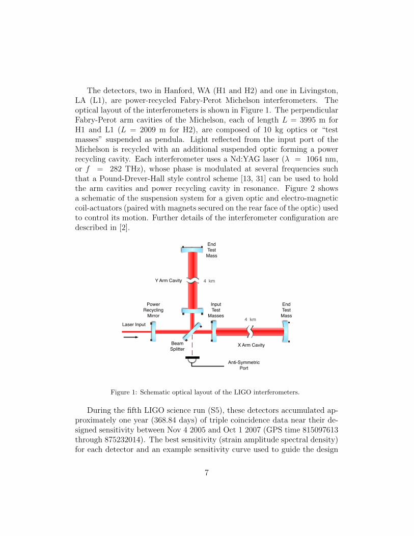
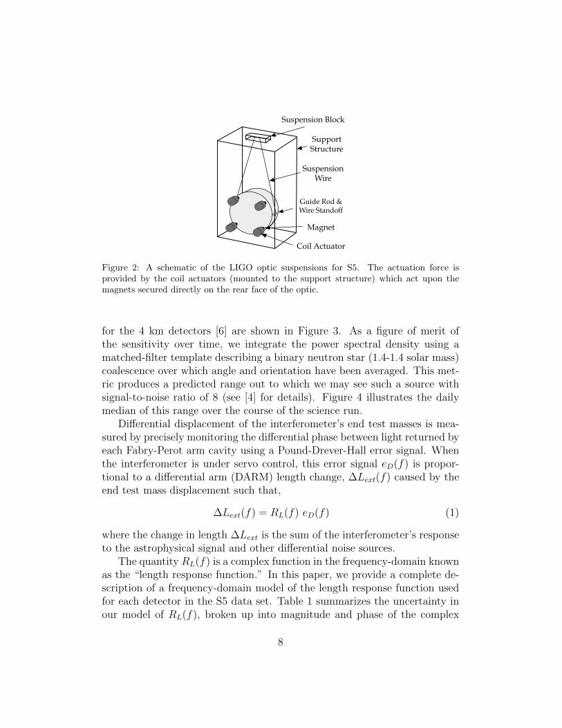
The detectors, two in Hanford, WA (H1 and H2) and one in Livingston,LA (L1), are power-recycled Fabry-Perot Michelson interferometers. Theoptical layout of the interferometers is shown in Figure 1. The perpendicularFabry-Perot arm cavities of the Michelson, each of length L = 3995 m forH1 and L1 (L = 2009 m for H2), are composed of 10 kg optics or “testmasses” suspended as pendula. Light reflected from the input port of theMichelson is recycled with an additional suspended optic forming a powerrecycling cavity. Each interferometer uses a Nd:YAG laser (λ = 1064 nm,or f = 282 THz), whose phase is modulated at several frequencies suchthat a Pound-Drever-Hall style control scheme [13, 31] can be used to holdthe arm cavities and power recycling cavity in resonance. Figure 2 showsa schematic of the suspension system for a given optic and electro-magneticcoil-actuators (paired with magnets secured on the rear face of the optic) usedto control its motion. Further details of the interferometer configuration aredescribed in [2].

4 km

4 km

Power

Recycling

Mirror

Beam

Splitter

Input

Test

Masses

End

Test

Mass

X Arm Cavity

Y Arm Cavity

Anti-Symmetric

Port

End

Test

Mass

Laser Input

Figure 1: Schematic optical layout of the LIGO interferometers.

During the fifth LIGO science run (S5), these detectors accumulated ap-proximately one year (368.84 days) of triple coincidence data near their de-signed sensitivity between Nov 4 2005 and Oct 1 2007 (GPS time 815097613through 875232014). The best sensitivity (strain amplitude spectral density)for each detector and an example sensitivity curve used to guide the design

7

Suspension Block

Support Structure

Suspension Wire

Magnet

Coil Actuator

Guide Rod & Wire Standoff

Figure 2: A schematic of the LIGO optic suspensions for S5. The actuation force isprovided by the coil actuators (mounted to the support structure) which act upon themagnets secured directly on the rear face of the optic.

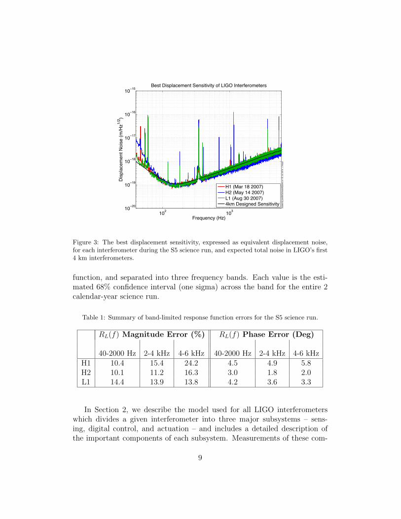
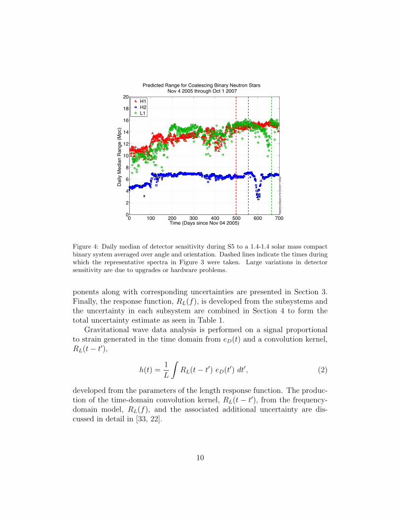
for the 4 km detectors [6] are shown in Figure 3. As a figure of merit ofthe sensitivity over time, we integrate the power spectral density using amatched-filter template describing a binary neutron star (1.4-1.4 solar mass)coalescence over which angle and orientation have been averaged. This met-ric produces a predicted range out to which we may see such a source withsignal-to-noise ratio of 8 (see [4] for details). Figure 4 illustrates the dailymedian of this range over the course of the science run.

Differential displacement of the interferometer’s end test masses is mea-sured by precisely monitoring the differential phase between light returned byeach Fabry-Perot arm cavity using a Pound-Drever-Hall error signal. Whenthe interferometer is under servo control, this error signal eD(f) is propor-tional to a differential arm (DARM) length change, ∆Lext(f) caused by theend test mass displacement such that,

∆Lext(f) = RL(f) eD(f) (1)

where the change in length ∆Lext is the sum of the interferometer’s responseto the astrophysical signal and other differential noise sources.

The quantity RL(f) is a complex function in the frequency-domain knownas the “length response function.” In this paper, we provide a complete de-scription of a frequency-domain model of the length response function usedfor each detector in the S5 data set. Table 1 summarizes the uncertainty inour model of RL(f), broken up into magnitude and phase of the complex

8

102

103

10!20

10!19

10!18

10!17

10!16

10!15

Best Displacement Sensitivity of LIGO Interferometers

Frequency (Hz)

Dis

pla

ce

me

nt

No

ise

(m

/Hz

1/2

)

cre

ate

d b

y p

lotS

5C

alib

rate

dS

pectr

a o

n 1

5!

Jul!

2010 , J

. K

issel

H1 (Mar 18 2007)H2 (May 14 2007)L1 (Aug 30 2007)4km Designed Sensitivity

Figure 3: The best displacement sensitivity, expressed as equivalent displacement noise,for each interferometer during the S5 science run, and expected total noise in LIGO’s first4 km interferometers.

function, and separated into three frequency bands. Each value is the esti-mated 68% confidence interval (one sigma) across the band for the entire 2calendar-year science run.

Table 1: Summary of band-limited response function errors for the S5 science run.

RL(f) Magnitude Error (%) RL(f) Phase Error (Deg)

40-2000 Hz 2-4 kHz 4-6 kHz 40-2000 Hz 2-4 kHz 4-6 kHzH1 10.4 15.4 24.2 4.5 4.9 5.8H2 10.1 11.2 16.3 3.0 1.8 2.0L1 14.4 13.9 13.8 4.2 3.6 3.3

In Section 2, we describe the model used for all LIGO interferometerswhich divides a given interferometer into three major subsystems – sens-ing, digital control, and actuation – and includes a detailed description ofthe important components of each subsystem. Measurements of these com-

9

0 100 200 300 400 500 600 7000

2

4

6

8

10

12

14

16

18

20

Predicted Range for Coalescing Binary Neutron Stars Nov 4 2005 through Oct 1 2007

Time (Days since Nov 04 2005)

Da

ily M

ed

ian

Ra

ng

e (

Mp

c)

cre

ate

d b

y w

ork

space o

n 1

5!

Jul!

2010 , J

. K

issel

H1H2L1

Figure 4: Daily median of detector sensitivity during S5 to a 1.4-1.4 solar mass compactbinary system averaged over angle and orientation. Dashed lines indicate the times duringwhich the representative spectra in Figure 3 were taken. Large variations in detectorsensitivity are due to upgrades or hardware problems.

ponents along with corresponding uncertainties are presented in Section 3.Finally, the response function, RL(f), is developed from the subsystems andthe uncertainty in each subsystem are combined in Section 4 to form thetotal uncertainty estimate as seen in Table 1.

Gravitational wave data analysis is performed on a signal proportionalto strain generated in the time domain from eD(t) and a convolution kernel,RL(t− t′),

h(t) =1

L

∫RL(t− t′) eD(t′) dt′, (2)

developed from the parameters of the length response function. The produc-tion of the time-domain convolution kernel, RL(t − t′), from the frequency-domain model, RL(f), and the associated additional uncertainty are dis-cussed in detail in [33, 22].

10

2. Model

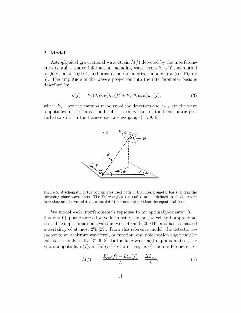
Astrophysical gravitational wave strain h(f) detected by the interferom-eters contains source information including wave forms h+,×(f), azimuthalangle φ, polar angle θ, and orientation (or polarization angle) ψ (see Figure5). The amplitude of the wave’s projection into the interferometer basis isdescribed by

h(f) = F×(θ, φ, ψ)h×(f) + F+(θ, φ, ψ)h+(f), (3)

where F×,+ are the antenna response of the detectors and h×,+ are the waveamplitudes in the “cross” and “plus” polarizations of the local metric per-turbations hµν in the transverse-traceless gauge [37, 9, 8].

!

ψ

"

x'

x

y

y'z

Figure 5: A schematic of the coordinates used both in the interferometer basis, and in theincoming plane wave basis. The Euler angles θ, φ and ψ are as defined in [9, 8], excepthere they are shown relative to the detector frame rather than the equatorial frame.

We model each interferometer’s repsonse to an optimally-oriented (θ =φ = ψ = 0), plus-polarized wave form using the long wavelength approxima-tion. The approximation is valid between 40 and 6000 Hz, and has associateduncertainty of at most 2% [29]. From this reference model, the detector re-sponse to an arbitrary waveform, orientation, and polarization angle may becalculated analytically [37, 9, 8]. In the long wavelength approximation, thestrain amplitude, h(f), in Fabry-Perot arm lengths of the interferometer is

h(f) =Lxext(f)− Lyext(f)

L=

∆LextL

. (4)

11

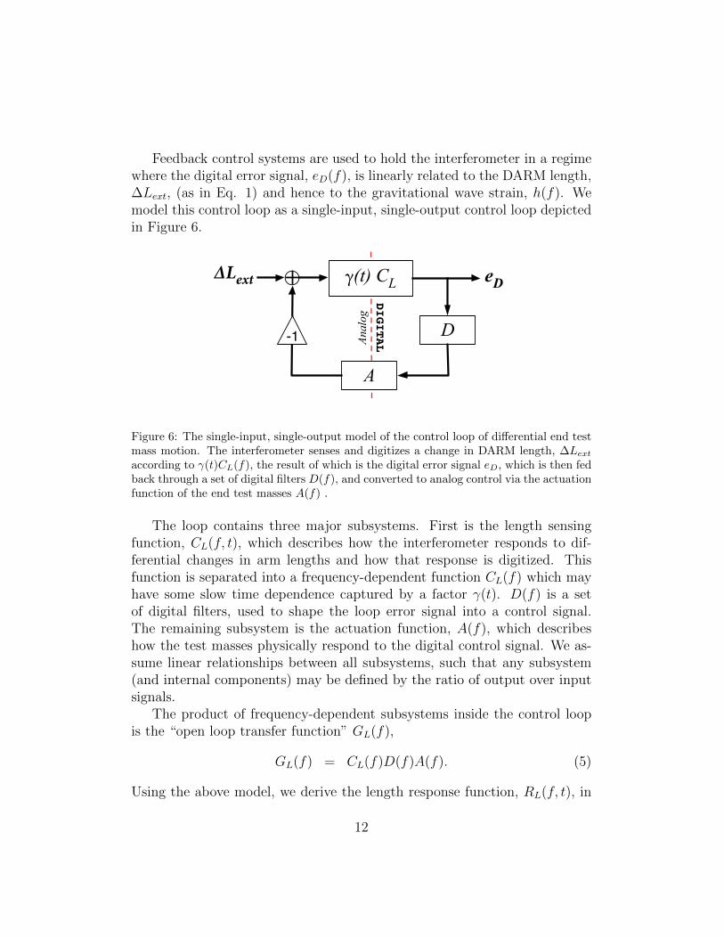
Feedback control systems are used to hold the interferometer in a regimewhere the digital error signal, eD(f), is linearly related to the DARM length,∆Lext, (as in Eq. 1) and hence to the gravitational wave strain, h(f). Wemodel this control loop as a single-input, single-output control loop depictedin Figure 6.

D

!(t) CL

A

!Lext eD

DIGITALA

na

log

-1

Figure 6: The single-input, single-output model of the control loop of differential end testmass motion. The interferometer senses and digitizes a change in DARM length, ∆Lextaccording to γ(t)CL(f), the result of which is the digital error signal eD, which is then fedback through a set of digital filters D(f), and converted to analog control via the actuationfunction of the end test masses A(f) .

The loop contains three major subsystems. First is the length sensingfunction, CL(f, t), which describes how the interferometer responds to dif-ferential changes in arm lengths and how that response is digitized. Thisfunction is separated into a frequency-dependent function CL(f) which mayhave some slow time dependence captured by a factor γ(t). D(f) is a setof digital filters, used to shape the loop error signal into a control signal.The remaining subsystem is the actuation function, A(f), which describeshow the test masses physically respond to the digital control signal. We as-sume linear relationships between all subsystems, such that any subsystem(and internal components) may be defined by the ratio of output over inputsignals.

The product of frequency-dependent subsystems inside the control loopis the “open loop transfer function” GL(f),

GL(f) = CL(f)D(f)A(f). (5)

Using the above model, we derive the length response function, RL(f, t), in

12

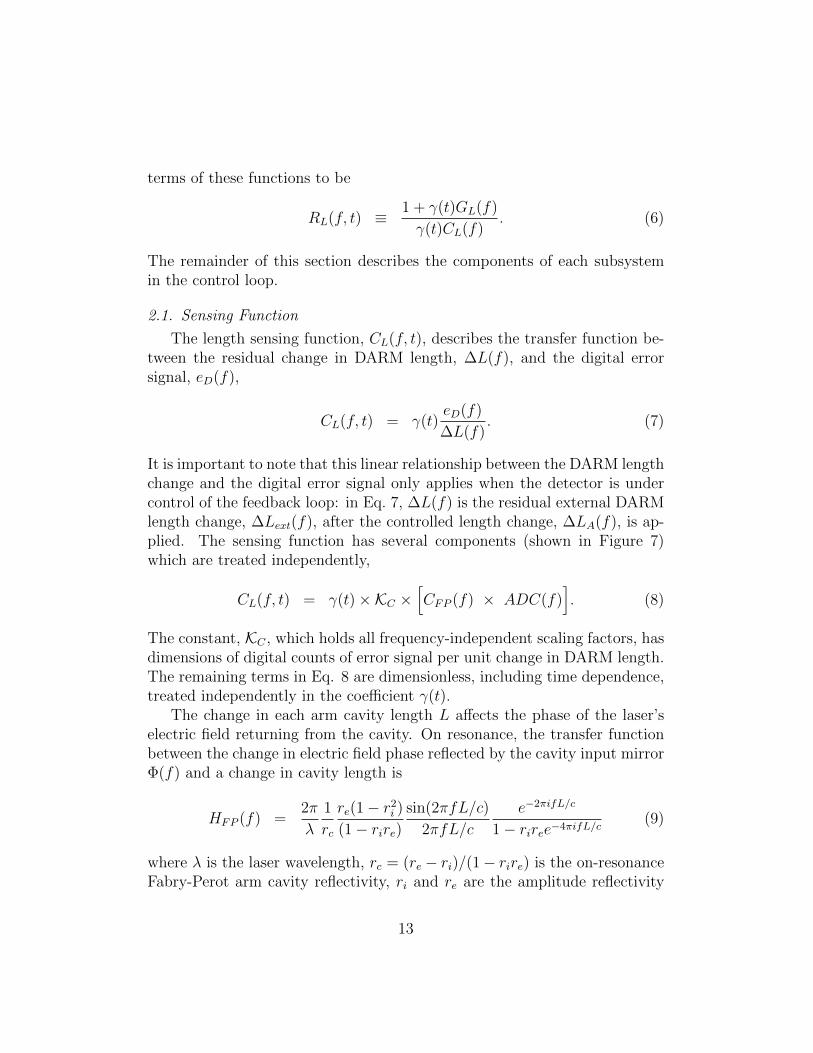
terms of these functions to be

RL(f, t) ≡ 1 + γ(t)GL(f)

γ(t)CL(f). (6)

The remainder of this section describes the components of each subsystemin the control loop.

2.1. Sensing Function

The length sensing function, CL(f, t), describes the transfer function be-tween the residual change in DARM length, ∆L(f), and the digital errorsignal, eD(f),

CL(f, t) = γ(t)eD(f)

∆L(f). (7)

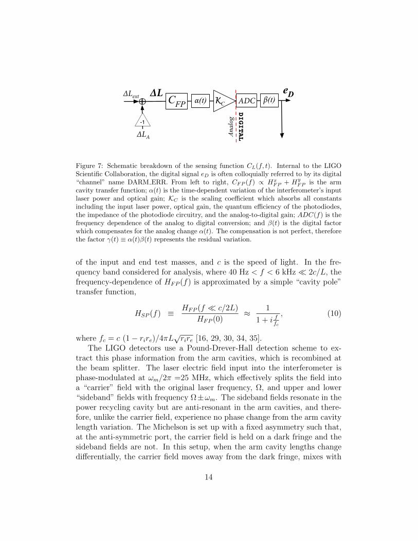
It is important to note that this linear relationship between the DARM lengthchange and the digital error signal only applies when the detector is undercontrol of the feedback loop: in Eq. 7, ∆L(f) is the residual external DARMlength change, ∆Lext(f), after the controlled length change, ∆LA(f), is ap-plied. The sensing function has several components (shown in Figure 7)which are treated independently,

CL(f, t) = γ(t)×KC ×[CFP (f) × ADC(f)

]. (8)

The constant, KC , which holds all frequency-independent scaling factors, hasdimensions of digital counts of error signal per unit change in DARM length.The remaining terms in Eq. 8 are dimensionless, including time dependence,treated independently in the coefficient γ(t).

The change in each arm cavity length L affects the phase of the laser’selectric field returning from the cavity. On resonance, the transfer functionbetween the change in electric field phase reflected by the cavity input mirrorΦ(f) and a change in cavity length is

HFP (f) =2π

λ

1

rc

re(1− r2i )

(1− rire)sin(2πfL/c)

2πfL/c

e−2πifL/c

1− riree−4πifL/c(9)

where λ is the laser wavelength, rc = (re − ri)/(1− rire) is the on-resonanceFabry-Perot arm cavity reflectivity, ri and re are the amplitude reflectivity

13

DIGITALA

nalog

eD!Lext

CFP "(t) #(t)ADCKC

!LA

!L

-1

Figure 7: Schematic breakdown of the sensing function CL(f, t). Internal to the LIGOScientific Collaboration, the digital signal eD is often colloquially referred to by its digital“channel” name DARM ERR. From left to right, CFP (f) ∝ Hx

FP + HyFP is the arm

cavity transfer function; α(t) is the time-dependent variation of the interferometer’s inputlaser power and optical gain; KC is the scaling coefficient which absorbs all constantsincluding the input laser power, optical gain, the quantum efficiency of the photodiodes,the impedance of the photodiode circuitry, and the analog-to-digital gain; ADC(f) is thefrequency dependence of the analog to digital conversion; and β(t) is the digital factorwhich compensates for the analog change α(t). The compensation is not perfect, thereforethe factor γ(t) ≡ α(t)β(t) represents the residual variation.

of the input and end test masses, and c is the speed of light. In the fre-quency band considered for analysis, where 40 Hz < f < 6 kHz 2c/L, thefrequency-dependence of HFP (f) is approximated by a simple “cavity pole”transfer function,

HSP (f) ≡ HFP (f c/2L)

HFP (0)≈ 1

1 + i ffc

, (10)

where fc = c (1− rire)/4πL√rire [16, 29, 30, 34, 35].

The LIGO detectors use a Pound-Drever-Hall detection scheme to ex-tract this phase information from the arm cavities, which is recombined atthe beam splitter. The laser electric field input into the interferometer isphase-modulated at ωm/2π =25 MHz, which effectively splits the field intoa “carrier” field with the original laser frequency, Ω, and upper and lower“sideband” fields with frequency Ω±ωm. The sideband fields resonate in thepower recycling cavity but are anti-resonant in the arm cavities, and there-fore, unlike the carrier field, experience no phase change from the arm cavitylength variation. The Michelson is set up with a fixed asymmetry such that,at the anti-symmetric port, the carrier field is held on a dark fringe and thesideband fields are not. In this setup, when the arm cavity lengths changedifferentially, the carrier field moves away from the dark fringe, mixes with

14

the sideband field at the antisymmetric port, and a beat signal at ωm isgenerated.

The power of the mixed field at the antisymmetric port (in Watts) issensed by four photodiodes. The photocurrent from these diodes is con-verted to voltage, and then demodulated at 25 MHz. This voltage signal(and therefore the change in DARM length) is proportional to power of theinput laser field, the “optical gain” (the product of Bessel functions of mod-ulation strength, the recycling cavity gain, the transmission of the sidebandsinto the antisymmetric port from the Michelson asymmetry, the reflectivityof the arm cavities for the carrier), the quantum efficiency of the photodi-odes, and the impedance of the photodiode circuitry [31, 16, 34, 35]. Thedemodulated voltage from the photodiodes is whitened, and anti-aliased withanalog circuitry and then digitized by an analog-to-digital converter whichscales the voltage to digital counts. The frequency dependence of the anti-aliasing filters and digitization process is folded into the function ADC(f).We absorb all proportionality and dimensions of this process into the singleconstant, KC , having dimensions of digital counts per meter of DARM testmass motion.

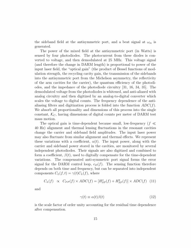
The optical gain is time-dependent because small, low-frequency (f 40 Hz) alignment and thermal lensing fluctuations in the resonant cavitieschange the carrier and sideband field amplitudes. The input laser powermay also fluctuate from similar alignment and thermal effects. We representthese variations with a coefficient, α(t). The input power, along with thecarrier and sideband power stored in the cavities, are monitored by severalindependent photodiodes. Their signals are also digitized and combined toform a coefficient, β(t), used to digitally compensate for the time-dependentvariations. The compensated anti-symmetric port signal forms the errorsignal for the DARM control loop, eD(f). The sensing function thereforedepends on both time and frequency, but can be separated into independentcomponents CL(f, t) = γ(t)CL(f), where

CL(f) ∝ CFP (f)× ADC(f) = [HxSP (f) +Hy

SP (f)]× ADC(f) (11)

and

γ(t) ≡ α(t)β(t) (12)

is the scale factor of order unity accounting for the residual time dependenceafter compensation.

15

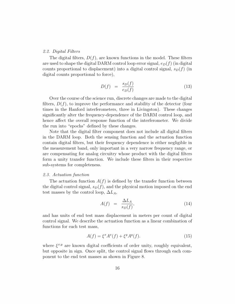
2.2. Digital Filters

The digital filters, D(f), are known functions in the model. These filtersare used to shape the digital DARM control loop error signal, eD(f) (in digitalcounts proportional to displacement) into a digital control signal, sD(f) (indigital counts proportional to force),

D(f) =sD(f)

eD(f)(13)

Over the course of the science run, discrete changes are made to the digitalfilters, D(f), to improve the performance and stability of the detector (fourtimes in the Hanford interferometers, three in Livingston). These changessignificantly alter the frequency-dependence of the DARM control loop, andhence affect the overall response function of the interferometer. We dividethe run into “epochs” defined by these changes.

Note that the digital filter component does not include all digital filtersin the DARM loop. Both the sensing function and the actuation functioncontain digital filters, but their frequency dependence is either negligible inthe measurement band, only important in a very narrow frequency range, orare compensating for analog circuitry whose product with the digital filtersform a unity transfer function. We include these filters in their respectivesub-systems for completeness.

2.3. Actuation function

The actuation function A(f) is defined by the transfer function betweenthe digital control signal, sD(f), and the physical motion imposed on the endtest masses by the control loop, ∆LA,

A(f) =∆LAsD(f)

, (14)

and has units of end test mass displacement in meters per count of digitalcontrol signal. We describe the actuation function as a linear combination offunctions for each test mass,

A(f) = ξxAx(f) + ξyAy(f). (15)

where ξx,y are known digital coefficients of order unity, roughly equivalent,but opposite in sign. Once split, the control signal flows through each com-ponent to the end test masses as shown in Figure 8.

16

DIGITAL

Analog

DAC

!LAsD

Px KAx ξx

x

DAx

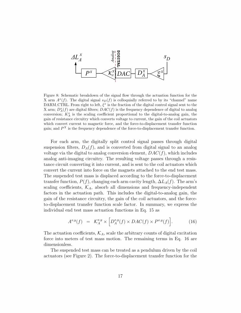
Figure 8: Schematic breakdown of the signal flow through the actuation function for theX arm Ax(f). The digital signal sD(f) is colloquially referred to by its “channel” nameDARM CTRL. From right to left, ξx is the fraction of the digital control signal sent to theX arm; Dx

A(f) are digital filters; DAC(f) is the frequency dependence of digital to analogconversion; Kx

A is the scaling coefficient proportional to the digital-to-analog gain, thegain of resistance circuitry which converts voltage to current, the gain of the coil actuatorswhich convert current to magnetic force, and the force-to-displacement transfer functiongain; and PX is the frequency dependence of the force-to-displacement transfer function.

For each arm, the digitally split control signal passes through digitalsuspension filters, DA(f), and is converted from digital signal to an analogvoltage via the digital to analog conversion element, DAC(f), which includesanalog anti-imaging circuitry. The resulting voltage passes through a resis-tance circuit converting it into current, and is sent to the coil actuators whichconvert the current into force on the magnets attached to the end test mass.The suspended test mass is displaced according to the force-to-displacementtransfer function, P (f), changing each arm cavity length, ∆LA(f). The arm’sscaling coefficients, KA, absorb all dimensions and frequency-independentfactors in the actuation path. This includes the digital-to-analog gain, thegain of the resistance circuitry, the gain of the coil actuators, and the force-to-displacement transfer function scale factor. In summary, we express theindividual end test mass actuation functions in Eq. 15 as

Ax,y(f) = Kx,yA ×[Dx,yA (f)×DAC(f)× P x,y(f)

]. (16)

The actuation coefficients, KA, scale the arbitrary counts of digital excitationforce into meters of test mass motion. The remaining terms in Eq. 16 aredimensionless.

The suspended test mass can be treated as a pendulum driven by the coilactuators (see Figure 2). The force-to-displacement transfer function for the

17

center of mass of a pendulum, Pcm(f), is

Pcm(f) ∝ 1

[f cm0 ]2 + i[fcm0 ]

Qcm f − f 2(17)

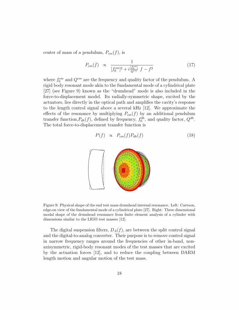
where f cm0 and Qcm are the frequency and quality factor of the pendulum. Arigid body resonant mode akin to the fundamental mode of a cylindrical plate[27] (see Figure 9) known as the “drumhead” mode is also included in theforce-to-displacement model. Its radially-symmetric shape, excited by theactuators, lies directly in the optical path and amplifies the cavity’s responseto the length control signal above a several kHz [12]. We approximate theeffects of the resonance by multiplying Pcm(f) by an additional pendulumtransfer function,Pdh(f), defined by frequency, fdh0 , and quality factor, Qdh.The total force-to-displacement transfer function is

P (f) ∝ Pcm(f)Pdh(f) (18)

LIGO

LIG

O-T

030086-00-D

5

3

9866

4

11225

Figure 9: Physical shape of the end test mass drumhead internal resonance. Left: Cartoon,edge-on view of the fundamental mode of a cylindrical plate [27]. Right: Three dimensionalmodal shape of the drumhead resonance from finite element analysis of a cylinder withdimensions similar to the LIGO test masses [12].

The digital suspension filters, DA(f), are between the split control signaland the digital-to-analog converter. Their purpose is to remove control signalin narrow frequency ranges around the frequencies of other in-band, non-axisymmetric, rigid-body resonant modes of the test masses that are excitedby the actuation forces [12], and to reduce the coupling between DARMlength motion and angular motion of the test mass.

18

3. Measurements

Each subsystem of the response function RL(f) is developed using mea-surements of key parameters in their modeled frequency dependence andtheir scaling coefficients. The digital filter subsystem is completely known;its frequency dependence and scaling coefficient are simply folded into themodel of the response function. The parameters of the frequency-dependentportions of the sensing and actuation subsystems may be obtained preciselyby direct measurement or are known from digital quantities and/or designschematics. As such, these parameters’ measurements will only be brieflydiscussed.

The detector’s sensing function behaves in a non-linear fashion when un-controlled, therefore we may only infer the linear model’s scaling coefficient,KC , from measurements of the detectors under closed control loops. Weinfer that the remaining magnitude ratio between our model and measure-ments of the open loop transfer function GL(fUGF ) as the sensing coefficientKC (where fUGF is the unity gain frequency of the DARM control loop).Other than the known frequency-independent magnitude of D(f), the openloop gain model’s magnitude is set by the actuation scale factor, KA. Thismakes it a crucial measurement in our model because it sets the frequency-independent magnitude of the entire response function. Measurements of theopen loop transfer function over the entire gravitational wave frequency bandare used to confirm that we have modeled the correct frequency dependenceof all subsystems. Finally, measurements of γ(t) track the time dependenceof the response function. The details of these measurements and respectiveuncertainty estimates are described below.

3.1. Actuation Function

The components of each arm’s actuation function, Kx,yA , DAC(f) andP x,y(f) are measured independently in a given detector. As with D(f),both ξx,y and Dx,y

A (f) are digital functions included in the model withoutuncertainty.

3.1.1. Actuation Scaling Coefficients, Kx,yAThe standard method for determining the actuation coefficients, Kx,yA ,

used for the fifth science run is an interferometric method known as the“free-swinging Michelson” technique; a culmination of several measurementswith the interferometer in non-standard configurations. The method uses

19

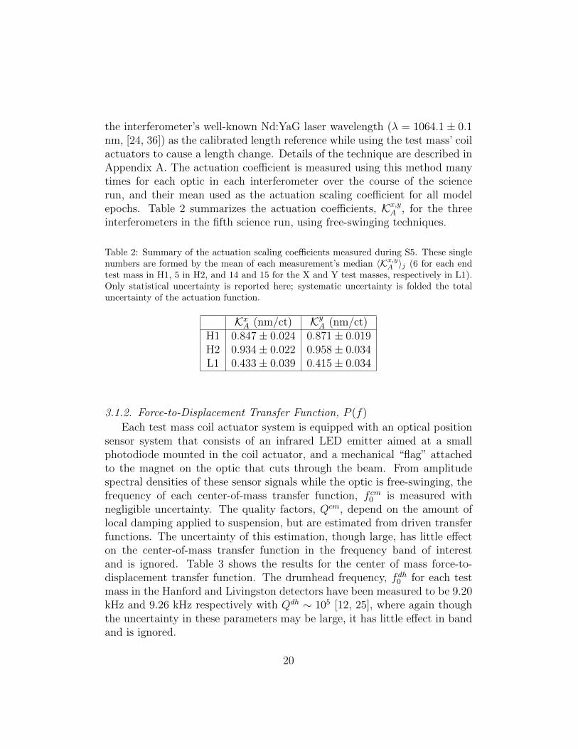
the interferometer’s well-known Nd:YaG laser wavelength (λ = 1064.1± 0.1nm, [24, 36]) as the calibrated length reference while using the test mass’ coilactuators to cause a length change. Details of the technique are described inAppendix A. The actuation coefficient is measured using this method manytimes for each optic in each interferometer over the course of the sciencerun, and their mean used as the actuation scaling coefficient for all modelepochs. Table 2 summarizes the actuation coefficients, Kx,yA , for the threeinterferometers in the fifth science run, using free-swinging techniques.

Table 2: Summary of the actuation scaling coefficients measured during S5. These singlenumbers are formed by the mean of each measurement’s median 〈Kx,yA 〉j (6 for each endtest mass in H1, 5 in H2, and 14 and 15 for the X and Y test masses, respectively in L1).Only statistical uncertainty is reported here; systematic uncertainty is folded the totaluncertainty of the actuation function.

KxA (nm/ct) KyA (nm/ct)H1 0.847± 0.024 0.871± 0.019H2 0.934± 0.022 0.958± 0.034L1 0.433± 0.039 0.415± 0.034

3.1.2. Force-to-Displacement Transfer Function, P (f)

Each test mass coil actuator system is equipped with an optical positionsensor system that consists of an infrared LED emitter aimed at a smallphotodiode mounted in the coil actuator, and a mechanical “flag” attachedto the magnet on the optic that cuts through the beam. From amplitudespectral densities of these sensor signals while the optic is free-swinging, thefrequency of each center-of-mass transfer function, f cm0 is measured withnegligible uncertainty. The quality factors, Qcm, depend on the amount oflocal damping applied to suspension, but are estimated from driven transferfunctions. The uncertainty of this estimation, though large, has little effecton the center-of-mass transfer function in the frequency band of interestand is ignored. Table 3 shows the results for the center of mass force-to-displacement transfer function. The drumhead frequency, fdh0 for each testmass in the Hanford and Livingston detectors have been measured to be 9.20kHz and 9.26 kHz respectively with Qdh ∼ 105 [12, 25], where again thoughthe uncertainty in these parameters may be large, it has little effect in bandand is ignored.

20

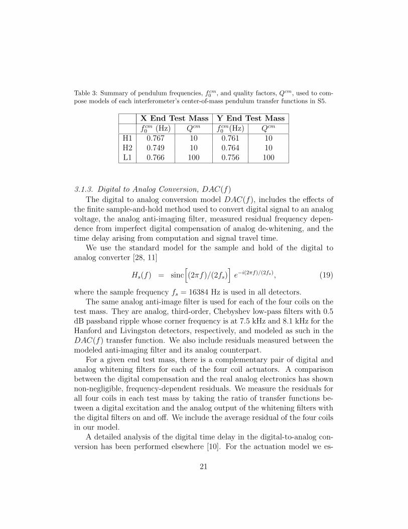
Table 3: Summary of pendulum frequencies, f cm0 , and quality factors, Qcm, used to com-pose models of each interferometer’s center-of-mass pendulum transfer functions in S5.

X End Test Mass Y End Test Massf cm0 (Hz) Qcm f cm0 (Hz) Qcm

H1 0.767 10 0.761 10H2 0.749 10 0.764 10L1 0.766 100 0.756 100

3.1.3. Digital to Analog Conversion, DAC(f)

The digital to analog conversion model DAC(f), includes the effects ofthe finite sample-and-hold method used to convert digital signal to an analogvoltage, the analog anti-imaging filter, measured residual frequency depen-dence from imperfect digital compensation of analog de-whitening, and thetime delay arising from computation and signal travel time.

We use the standard model for the sample and hold of the digital toanalog converter [28, 11]

Hs(f) = sinc[(2πf)/(2fs)

]e−i(2πf)/(2fs), (19)

where the sample frequency fs = 16384 Hz is used in all detectors.The same analog anti-image filter is used for each of the four coils on the

test mass. They are analog, third-order, Chebyshev low-pass filters with 0.5dB passband ripple whose corner frequency is at 7.5 kHz and 8.1 kHz for theHanford and Livingston detectors, respectively, and modeled as such in theDAC(f) transfer function. We also include residuals measured between themodeled anti-imaging filter and its analog counterpart.

For a given end test mass, there is a complementary pair of digital andanalog whitening filters for each of the four coil actuators. A comparisonbetween the digital compensation and the real analog electronics has shownnon-negligible, frequency-dependent residuals. We measure the residuals forall four coils in each test mass by taking the ratio of transfer functions be-tween a digital excitation and the analog output of the whitening filters withthe digital filters on and off. We include the average residual of the four coilsin our model.

A detailed analysis of the digital time delay in the digital-to-analog con-version has been performed elsewhere [10]. For the actuation model we es-

21

timate the time delay from our model of the open loop transfer function(attributing all residual delay in the loop to the actuation function), andassign a fixed delay to each epoch.

3.1.4. Actuation Uncertainty, σAThe digital suspension filters, DA(f), have well-known digital transfer

functions, which are included in the model without an uncertainty. Themodel of force-to-displacement transfer function, P (f), and digital-to-analogconversion, DAC(f), are derived from quantities with negligible uncertainty.Hence, the uncertainty estimate for the actuation function is derived entirelyfrom measurements of the actuation scaling coefficient, KA.

The actuation coefficient is measured using a series of complex transferfunctions taken to be frequency independent as described in Appendix A.We take advantage of this fact by estimating the frequency-independent un-certainty in the overall actuation function from the statistical uncertainty ofall free-swinging Michelson measurements. For magnitude, we include a sys-tematic uncertainty originating from an incomplete model of the actuationfrequency-dependence, such that the total actuation uncertainty is(

σ|A||A|

)2

=

(σ|KA|

|KA|

)2

+

(σ(r/a)

(r/a)

)2

(20)

σ2φA

= σ2φKA

. (21)

The statistical uncertainties, σ|KA|/|KA| and σφKA, are the quadrature sum

of the scaling coefficient uncertainty from each test mass, as measured by thefree-swinging Michelson technique. For each optic’s coefficient, we estimatethe uncertainty by taking the larger value of either the standard deviationof all measurement medians, or the mean of all measurement uncertaintiesdivided by the square root of the number of frequency points in a given mea-surement. These two numbers should be roughly the same if the measuredquantity followed a Gaussian distribution around some real mean value andstationary in time. For all optics, in all interferometers, in both magnitudeand phase, these two quantities are not similar, implying that the measure-ments do not arise from a parent Gaussian distribution. We attribute this tothe quantity changing over time, or a systematic error in our measurementtechnique that varies with time. Later studies of the free-swinging Michelsontechnique have revealed that the probable source of this time variation is ourassumption that the optical gain of the simple Michelson remains constantover the measurement suite (see Appendix A).

22

We have folded in an additional σ(r/a)/(r/a) = 4% systematic error inmagnitude for the Hanford detectors only. This correction results from thefollowing systematic difference between the Hanford and Livingston free-swinging Michelson measurement setup. Analog suspension filters, commonto all detectors, are used to increase the dynamic range of the coil actuatorsduring initial control of the test masses. When optic motions are sufficientlysmall enough to keep the cavity arms on resonance, they are turned off andleft off as the detectors approach designed sensitivity [2, 14]. These additionalsuspension filters were left in place for the Hanford measurements in order toobtain better signal-to-noise ratios for the driven transfer functions describedin Appendix A. The filters’ color had been compensated with digital filters,but the average residual frequency dependence is roughly 4% for both endtest masses in H1 and H2.

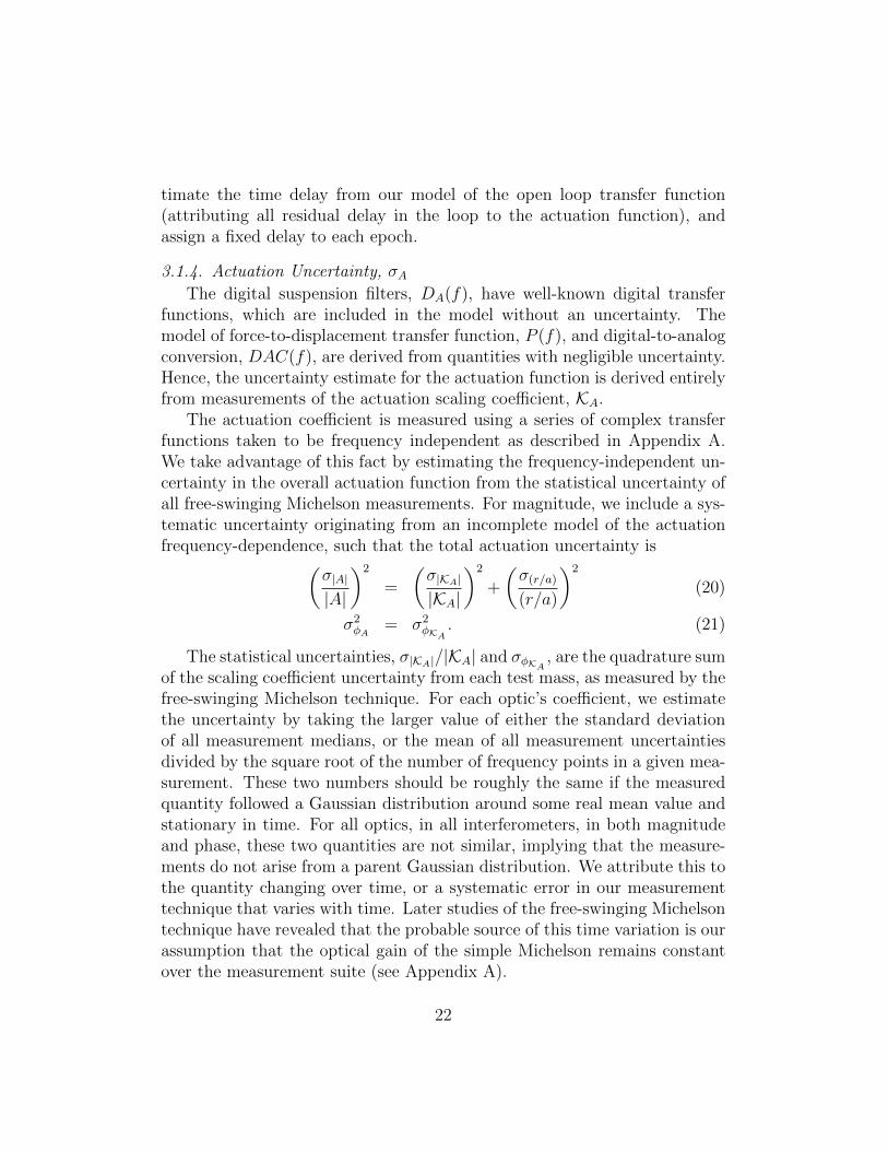
The total uncertainty for each interferometer’s actuation function, as de-scribed in Eq. 21, is shown in Figure 10. These estimates include statisticaland known systematic uncertainties. To investigate potential unknown sys-tematic uncertainties in the actuation functions we applied two fundamen-tally different calibration methods. The results of these investigations aredescribed in section 5.

102

103

00.020.040.060.08

0.10.120.14

S5 Actuation Function Uncertainty

Frequency (Hz)Rel

ativ

e M

agni

tude

Unc

erta

inty

102

103

0

1

2

3

4

5

Pha

se U

ncer

tain

ty (

deg)

Frequency (Hz)

crea

ted

by m

akeb

inne

dact

erro

r on

15−

Jul−

2010

, J.

Kis

sel

H1H2L1

Figure 10: Summary of the actuation uncertainty for all detectors in S5.

23

3.2. Sensing Function

The components of the sensing function, KC , CFP (f), and ADC(f) aredescribed in §2.1. The frequency-dependent components are developed frommeasured parameters with negligible uncertainties, and KC is obtained asdescribed above. The techniques used to obtain the parameters are describedbelow.

3.2.1. Sensing Scaling Coefficient, KCIn principle, the scaling coefficient KC is also composed of many inde-

pendently measurable parameters as described in §2.1. In practice, thesecomponents (specifically components of the optical gain) are difficult to mea-sure independently as the interferometer must be controlled into the linearregime before precise measurements can be made. The scaling coefficient forthe other subsystems are either measured (in the actuation) or known (inthe digital filters). We take advantage of this by developing the remainderof sensing subsystem (i.e. its frequency-dependence), forming the frequency-dependent loop model scaled by the measured actuation and known digitalfilter gain, and assume the remaining gain difference between a measurementof open loop transfer function and the model is entirely the sensing scalefactor. Results will be discussed in §3.3.

3.2.2. Fabry-Perot Cavity Response, CFP (f)

Our model of the Fabry-Perot Michelson frequency response is the sum ofthe response from each arm as in Eq. 11. Using the single pole approximation(Eq. 10), the frequency response of each arm cavity Hx,y

SP (f) can be calculatedexplicitly using a single measured quantity, the cavity pole frequency fc. Wecompute fc by measuring the light storage time τ = 1/(4πfc) in each cavity.

A single measurement of the storage time is performed by aligning asingle arm of the interferometer (as in the right panel of Figure A.17) andholding the cavity on resonance using the coil actuators. Then, the powertransmitted through that arm is recorded as we rapidly take the cavity outof resonance. We fit the resulting time series to a simple exponential decay,whose time constant is the light storage time in the cavity. This measurementis performed several times per arm, and the average light storage time is usedto calculate the cavity pole frequency. Table 4 shows the values of fc used ineach model.

24

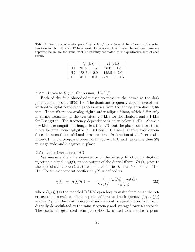
Table 4: Summary of cavity pole frequencies fc used in each interferometer’s sensingfunction in S5. H1 and H2 have used the average of each arm, hence their numbersreported below are the same, with uncertainty estimated as the quadrature sum of eachresult.

fxc (Hz) f yc (Hz)H1 85.6 ± 1.5 85.6 ± 1.5H2 158.5 ± 2.0 158.5 ± 2.0L1 85.1 ± 0.8 82.3 ± 0.5 Hz

3.2.3. Analog to Digital Conversion, ADC(f)

Each of the four photodiodes used to measure the power at the darkport are sampled at 16384 Hz. The dominant frequency dependence of thisanalog-to-digital conversion process arises from the analog anti-aliasing fil-ters. These filters are analog eighth order elliptic filters, which differ onlyin corner frequency at the two sites: 7.5 kHz for the Hanford and 8.1 kHzfor Livingston. The frequency dependence is unity below 1 kHz. Above afew kHz, the magnitude changes less than 2%, but the phase loss from thesefilters becomes non-negligible (> 180 deg). The residual frequency depen-dence between this model and measured transfer function of the filter is alsoincluded. The discrepancy occurs only above 1 kHz and varies less than 2%in magnitude and 5 degrees in phase.

3.2.4. Time Dependence, γ(t)

We measure the time dependence of the sensing function by digitallyinjecting a signal, scl(f), at the output of the digital filters, D(f), prior tothe control signal, sD(f), at three line frequencies fcl near 50, 400, and 1100Hz. The time-dependent coefficient γ(t) is defined as

γ(t) = α(t)β(t) = − 1

GL(fcl)

sD(fcl)− scl(fcl)sD(fcl)

, (22)

where GL(fcl) is the modeled DARM open loop transfer function at the ref-erence time in each epoch at a given calibration line frequency, fcl; scl(fcl)and sD(fcl) are the excitation signal and the control signal, respectively, eachdigitally demodulated at the same frequency and averaged over 60 seconds.The coefficient generated from fcl ≈ 400 Hz is used to scale the response

25

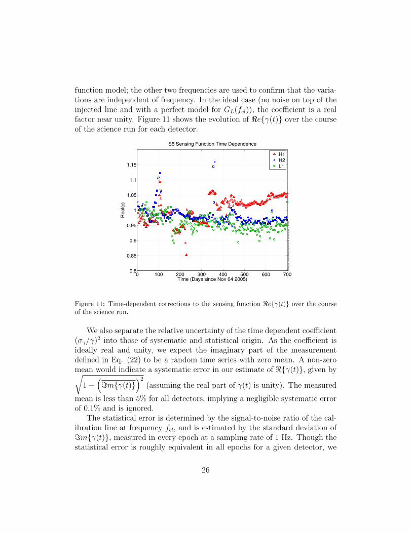
function model; the other two frequencies are used to confirm that the varia-tions are independent of frequency. In the ideal case (no noise on top of theinjected line and with a perfect model for GL(fcl)), the coefficient is a realfactor near unity. Figure 11 shows the evolution of <eγ(t) over the courseof the science run for each detector.

0 100 200 300 400 500 600 7000.8

0.85

0.9

0.95

1

1.05

1.1

1.15

S5 Sensing Function Time Dependence

Time (Days since Nov 04 2005)

Re

al(!)

cre

ate

d b

y p

lotS

5V

4tim

edependence o

n 1

5!

Jul!

2010 , J

. K

issel

H1H2L1

Figure 11: Time-dependent corrections to the sensing function <eγ(t) over the courseof the science run.

We also separate the relative uncertainty of the time dependent coefficient(σγ/γ)2 into those of systematic and statistical origin. As the coefficient isideally real and unity, we expect the imaginary part of the measurementdefined in Eq. (22) to be a random time series with zero mean. A non-zeromean would indicate a systematic error in our estimate of <γ(t), given by√

1−(=mγ(t)

)2

(assuming the real part of γ(t) is unity). The measured

mean is less than 5% for all detectors, implying a negligible systematic errorof 0.1% and is ignored.

The statistical error is determined by the signal-to-noise ratio of the cal-ibration line at frequency fcl, and is estimated by the standard deviation of=mγ(t), measured in every epoch at a sampling rate of 1 Hz. Though thestatistical error is roughly equivalent in all epochs for a given detector, we

26

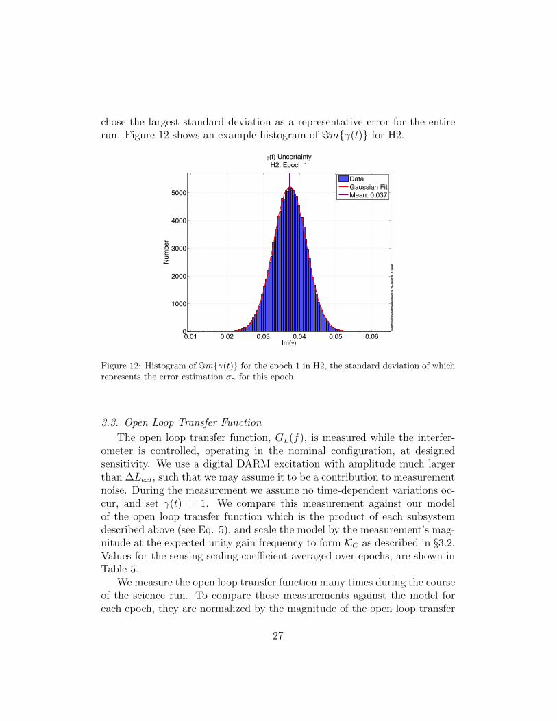
chose the largest standard deviation as a representative error for the entirerun. Figure 12 shows an example histogram of =mγ(t) for H2.

0.01 0.02 0.03 0.04 0.05 0.060

1000

2000

3000

4000

5000

!(t) Uncertainty

H2, Epoch 1

Im(!)

Num

ber

cre

ate

d b

y p

lotS

5V

4tim

ed

ep

en

de

nce

on

15!

Ju

l!2

01

0 ,

J.

Kis

se

lcre

ate

d b

y p

lotS

5V

4tim

ed

ep

en

de

nce

on

15!

Ju

l!2

01

0 ,

J.

Kis

se

l

Data

Gaussian Fit

Mean: 0.037

Figure 12: Histogram of =mγ(t) for the epoch 1 in H2, the standard deviation of whichrepresents the error estimation σγ for this epoch.

3.3. Open Loop Transfer Function

The open loop transfer function, GL(f), is measured while the interfer-ometer is controlled, operating in the nominal configuration, at designedsensitivity. We use a digital DARM excitation with amplitude much largerthan ∆Lext, such that we may assume it to be a contribution to measurementnoise. During the measurement we assume no time-dependent variations oc-cur, and set γ(t) = 1. We compare this measurement against our modelof the open loop transfer function which is the product of each subsystemdescribed above (see Eq. 5), and scale the model by the measurement’s mag-nitude at the expected unity gain frequency to form KC as described in §3.2.Values for the sensing scaling coefficient averaged over epochs, are shown inTable 5.

We measure the open loop transfer function many times during the courseof the science run. To compare these measurements against the model foreach epoch, they are normalized by the magnitude of the open loop transfer

27

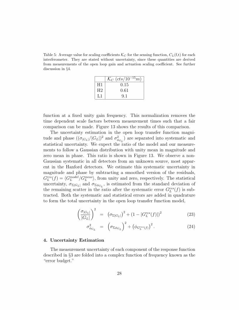
Table 5: Average value for scaling coefficients KC for the sensing function, CL(f,t) for eachinterferometer. They are stated without uncertainty, since these quantities are derivedfrom measurements of the open loop gain and actuation scaling coefficient. See furtherdiscussion in §4.

KC (cts/10−15m)H1 0.15H2 0.61L1 9.1

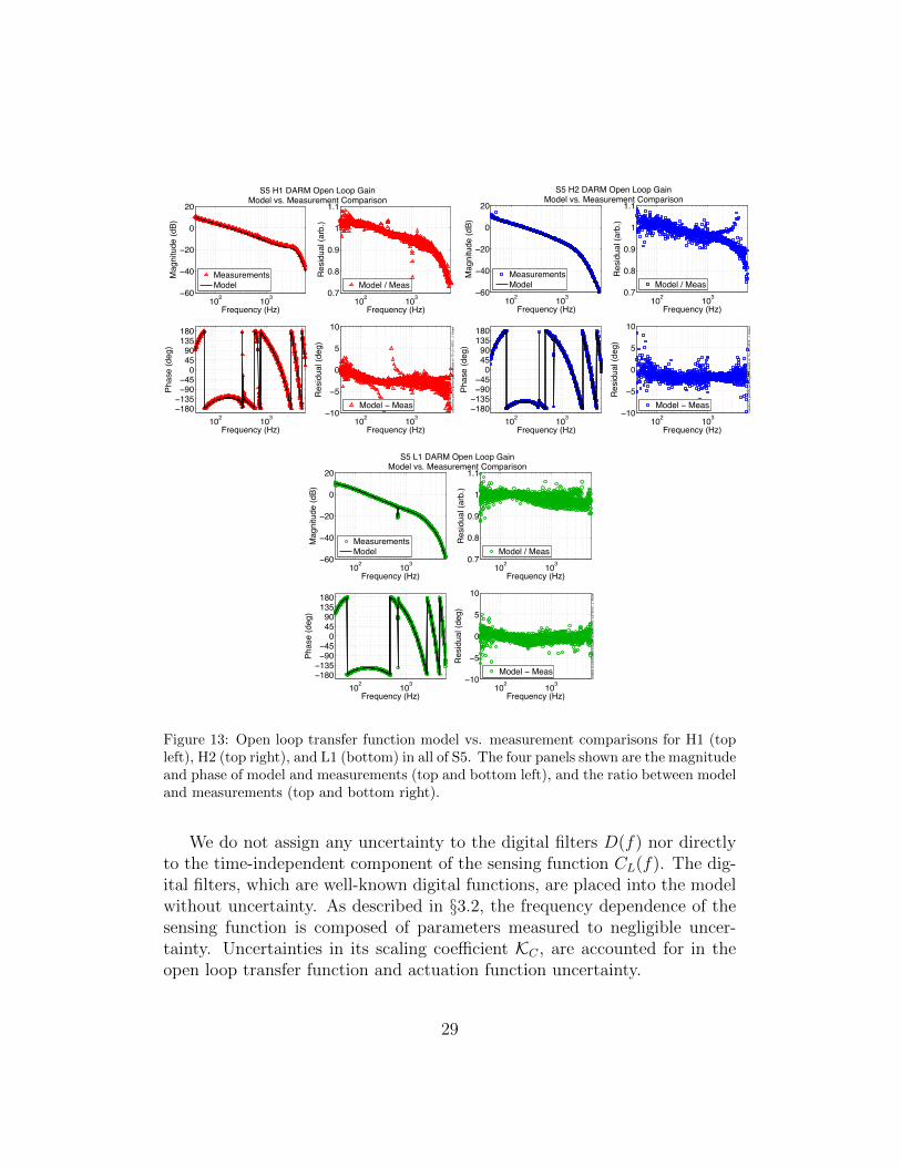
function at a fixed unity gain frequency. This normalization removes thetime dependent scale factors between measurement times such that a faircomparison can be made. Figure 13 shows the results of this comparison.

The uncertainty estimation in the open loop transfer function magni-tude and phase ((σ|GL|/|GL|)2 and σ2

φGL) are separated into systematic and

statistical uncertainty. We expect the ratio of the model and our measure-ments to follow a Gaussian distribution with unity mean in magnitude andzero mean in phase. This ratio is shown in Figure 13. We observe a non-Gaussian systematic in all detectors from an unknown source, most appar-ent in the Hanford detectors. We estimate this systematic uncertainty inmagnitude and phase by subtracting a smoothed version of the residuals,GresL (f) = 〈Gmodel

L /GmeasL 〉, from unity and zero, respectively. The statistical

uncertainty, σΣ|GL| and σΣφGL, is estimated from the standard deviation of

the remaining scatter in the ratio after the systematic error GresL (f) is sub-

tracted. Both the systematic and statistical errors are added in quadratureto form the total uncertainty in the open loop transfer function model,(

σ|GL|

|GL|

)2

=(σΣ|GL|

)2+ (1− |Gres

L (f)|)2 (23)

σ2φGL

=(σΣφGL

)2

+(φGres

L (f)

)2. (24)

4. Uncertainty Estimation

The measurement uncertainty of each component of the response functiondescribed in §3 are folded into a complex function of frequency known as the“error budget.”

28

S5 H1 DARM Open Loop GainModel vs. Measurement Comparison

102

103

!60

!40

!20

0

20

Frequency (Hz)

Ma

gn

itu

de

(d

B)

MeasurementsModel

102

103

0.7

0.8

0.9

1

1.1

Re

sid

ua

l (a

rb.)

Frequency (Hz)

Model / Meas

102

103

!180!135!90!45

04590

135180

Ph

ase

(d

eg

)

Frequency (Hz)10

210

3!10

!5

0

5

10R

esid

ua

l (d

eg

)

Frequency (Hz)

cre

ate

d b

y p

lotS

5openlo

opg

ain

mea

sts

on 1

5!

Jul!

2010 ,

J. K

issel

Model ! Meas

S5 H2 DARM Open Loop GainModel vs. Measurement Comparison

102

103

!60

!40

!20

0

20

Frequency (Hz)

Ma

gn

itu

de

(d

B)

MeasurementsModel

102

103

0.7

0.8

0.9

1

1.1

Re

sid

ua

l (a

rb.)

Frequency (Hz)

Model / Meas

102

103

!180!135!90!45

04590

135180

Ph

ase

(d

eg

)

Frequency (Hz)10

210

3!10

!5

0

5

10

Re

sid

ua

l (d

eg

)

Frequency (Hz)

cre

ate

d b

y p

lotS

5o

pe

nlo

op

ga

inm

ea

sts

on

15!

Ju

l!2

01

0 ,

J.

Kis

se

l

Model ! Meas

S5 L1 DARM Open Loop GainModel vs. Measurement Comparison

102

103

!60

!40

!20

0

20

Frequency (Hz)

Ma

gn

itu

de

(d

B)

MeasurementsModel

102

103

0.7

0.8

0.9

1

1.1

Resid

ual (a

rb.)

Frequency (Hz)

Model / Meas

102

103

!180!135!90!45

04590

135180

Ph

ase

(d

eg

)

Frequency (Hz)10

210

3!10

!5

0

5

10

Resid

ua

l (d

eg)

Frequency (Hz)

cre

ate

d b

y p

lotS

5ope

nlo

opgain

measts

on 1

5!

Jul!

20

10 , J

. K

issel

Model ! Meas

Figure 13: Open loop transfer function model vs. measurement comparisons for H1 (topleft), H2 (top right), and L1 (bottom) in all of S5. The four panels shown are the magnitudeand phase of model and measurements (top and bottom left), and the ratio between modeland measurements (top and bottom right).

We do not assign any uncertainty to the digital filters D(f) nor directlyto the time-independent component of the sensing function CL(f). The dig-ital filters, which are well-known digital functions, are placed into the modelwithout uncertainty. As described in §3.2, the frequency dependence of thesensing function is composed of parameters measured to negligible uncer-tainty. Uncertainties in its scaling coefficient KC , are accounted for in theopen loop transfer function and actuation function uncertainty.

29

The uncertainties of the remaining quantities in the response functionA(f), GL(f), and γ(t) are treated as uncorrelated. If the uncertainties arecompletely correlated (i.e. there are none in CL(f)), the covariant terms inthe estimation reduce the overall estimate of the response function uncer-tainty [23]. Since we do not have an independent estimate of the uncertaintyin the sensing function, we adopt this conservative estimate.

We re-write the response function in terms of the measured quantities towhich we assign uncertainty,

RL(f, t) = A(f)D(f)1 + γ(t)GL(f)

γ(t)GL(f)(25)

and separate into magnitude and phase (dropping terms which include theuncertainty in D(f)),

|RL| =

√(|A|γ|GL|

)2 [1 + (γ|GL|)2 + 2γ|GL| cos (φGL

)], (26)

φRL= arctan

(γ|GL| sin (φA) + sin (φA − φGL

)

γ|GL| cos (φA) + cos (φA − φGL)

), (27)

such that the relative uncertainty in magnitude and absolute uncertainty inphase are(

σ|RL|

|RL|

)2

=

(σ|A||A|

)2

+ <eW2

(σ|GL|

|GL|

)2

+ =mW2σ2φGL

+ <eW2

(σγγ

)2

(28)

σ2φRL

= σ2φA

+ =mW2

(σ|GL|

|GL|

)2

+ <eW2 σ2φGL

+ =mW2

(σγγ

)2

, (29)

where we define W ≡ 1/(1 +GL) [23]. Each uncertainty component in Eqs.28 and 29 is assumed to be the same over the course of the science run(independent of epochs). However, the complex coefficient W is different foreach epoch.

30

Our calculation of the response function includes the open loop transferfunction model which is approximated by replacing the complete cavity re-sponse HFP (f) (Eq. 9) with the single pole transfer function HSP (f) (Eq.10) in the sensing function subsystem. We include the ratio of the responsefunction calculated with and without the correct cavity response in our errorbudget,

RFPL (f)

RSPL (f)

=1 + (HFP/HSP )GL(f)

1 +GL(f)(30)

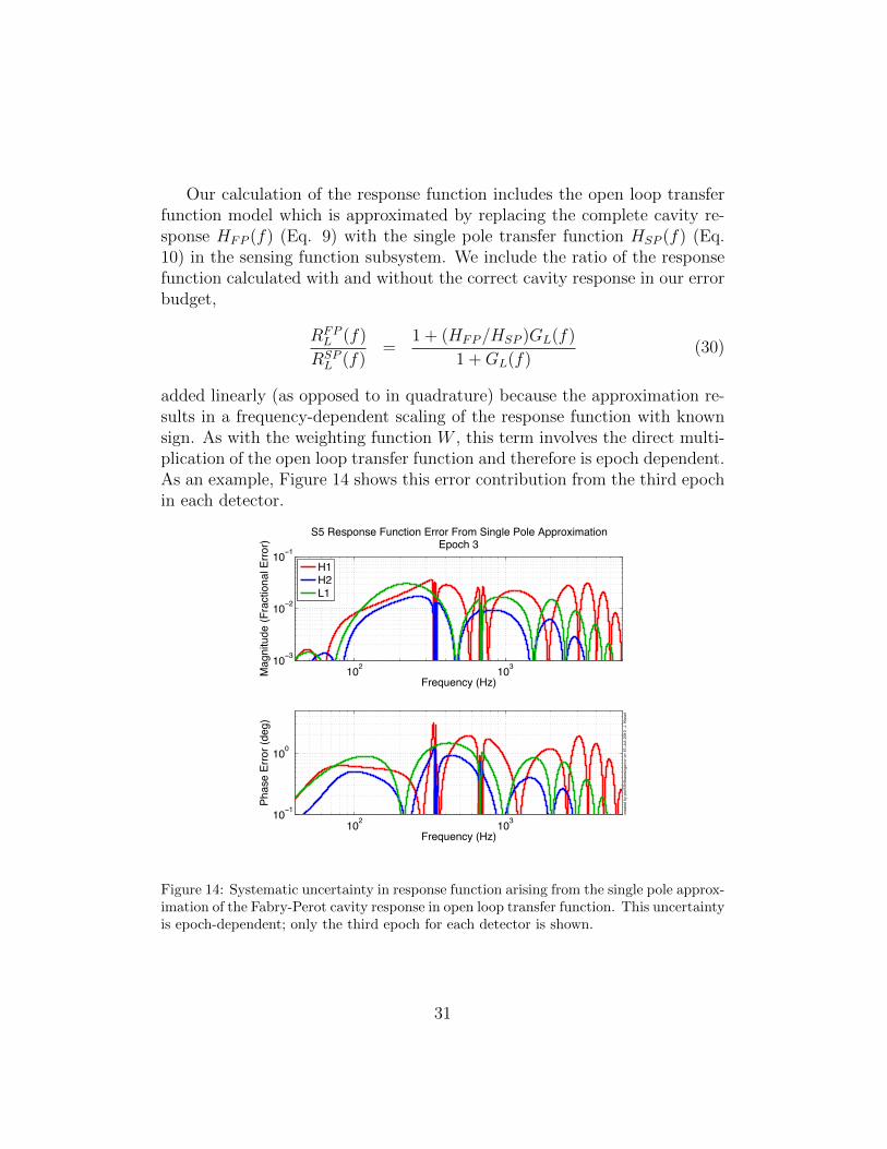
added linearly (as opposed to in quadrature) because the approximation re-sults in a frequency-dependent scaling of the response function with knownsign. As with the weighting function W , this term involves the direct multi-plication of the open loop transfer function and therefore is epoch dependent.As an example, Figure 14 shows this error contribution from the third epochin each detector.

102

103

10!3

10!2

10!1

S5 Response Function Error From Single Pole ApproximationEpoch 3

Frequency (Hz)

Ma

gnitude

(F

ractio

nal E

rror)

H1H2L1

102

103

10!1

100

Frequency (Hz)

Pha

se

Err

or

(deg)

cre

ate

d b

y p

lotS

5hflfs

ensin

gerr

or

on 1

5!

Jul!

2010 , J

. K

issel

Figure 14: Systematic uncertainty in response function arising from the single pole approx-imation of the Fabry-Perot cavity response in open loop transfer function. This uncertaintyis epoch-dependent; only the third epoch for each detector is shown.

31

5. Results

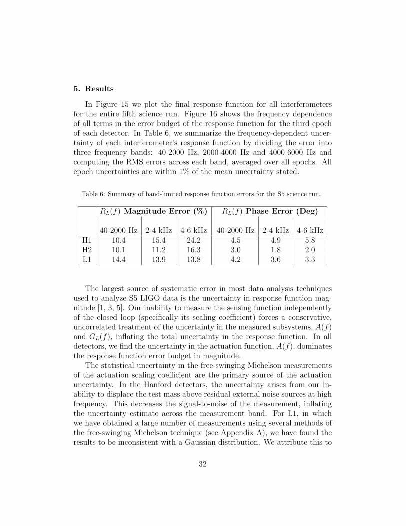
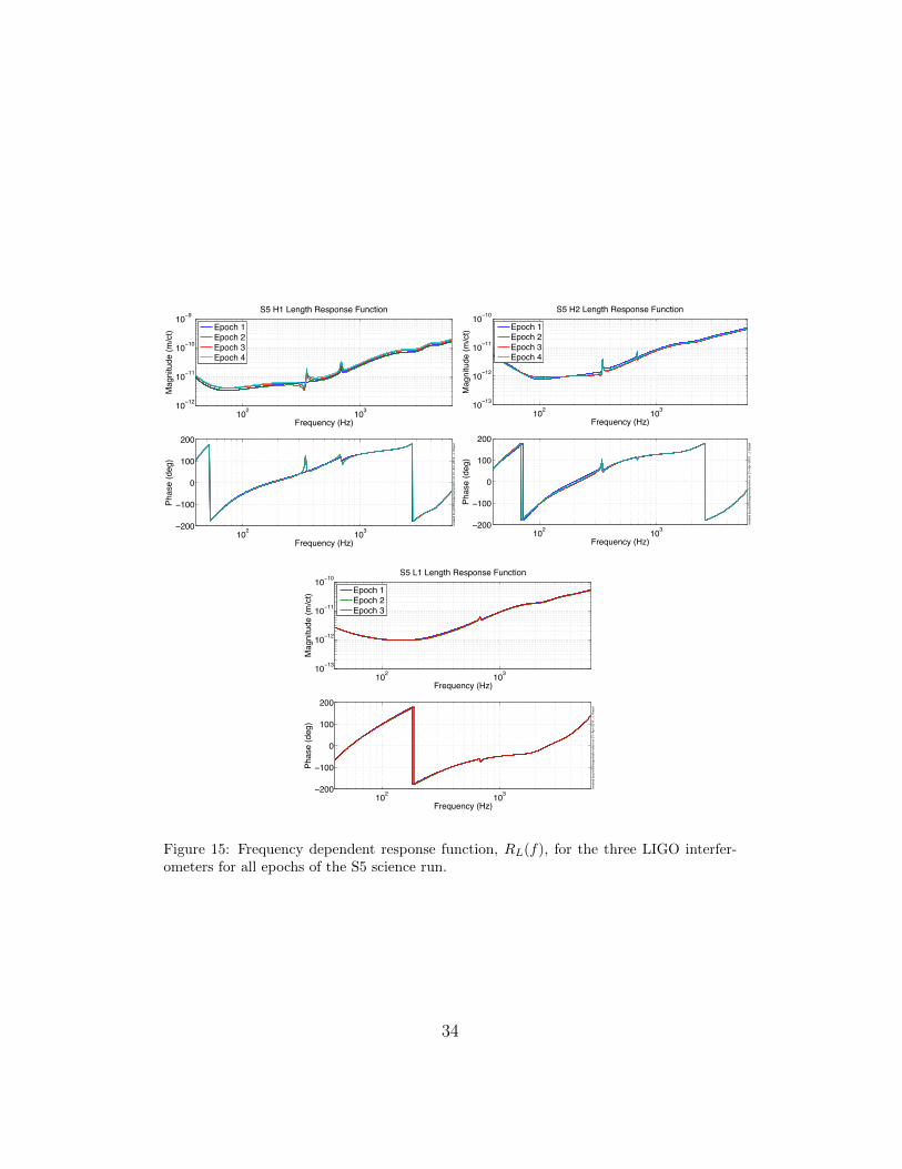
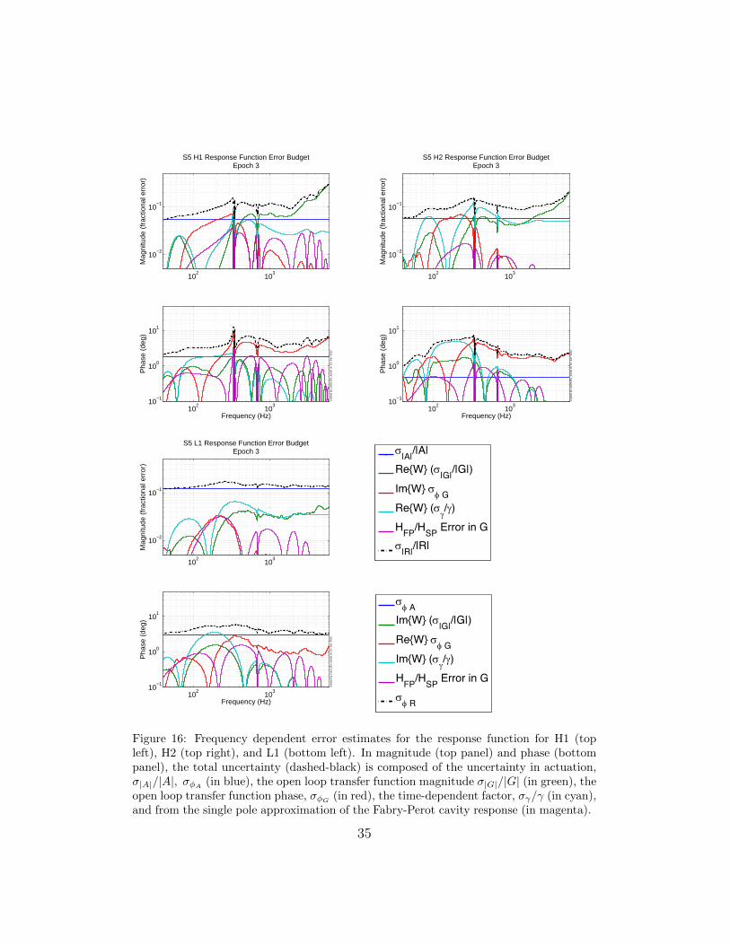
In Figure 15 we plot the final response function for all interferometersfor the entire fifth science run. Figure 16 shows the frequency dependenceof all terms in the error budget of the response function for the third epochof each detector. In Table 6, we summarize the frequency-dependent uncer-tainty of each interferometer’s response function by dividing the error intothree frequency bands: 40-2000 Hz, 2000-4000 Hz and 4000-6000 Hz andcomputing the RMS errors across each band, averaged over all epochs. Allepoch uncertainties are within 1% of the mean uncertainty stated.

Table 6: Summary of band-limited response function errors for the S5 science run.

RL(f) Magnitude Error (%) RL(f) Phase Error (Deg)

40-2000 Hz 2-4 kHz 4-6 kHz 40-2000 Hz 2-4 kHz 4-6 kHzH1 10.4 15.4 24.2 4.5 4.9 5.8H2 10.1 11.2 16.3 3.0 1.8 2.0L1 14.4 13.9 13.8 4.2 3.6 3.3

The largest source of systematic error in most data analysis techniquesused to analyze S5 LIGO data is the uncertainty in response function mag-nitude [1, 3, 5]. Our inability to measure the sensing function independentlyof the closed loop (specifically its scaling coefficient) forces a conservative,uncorrelated treatment of the uncertainty in the measured subsystems, A(f)and GL(f), inflating the total uncertainty in the response function. In alldetectors, we find the uncertainty in the actuation function, A(f), dominatesthe response function error budget in magnitude.

The statistical uncertainty in the free-swinging Michelson measurementsof the actuation scaling coefficient are the primary source of the actuationuncertainty. In the Hanford detectors, the uncertainty arises from our in-ability to displace the test mass above residual external noise sources at highfrequency. This decreases the signal-to-noise of the measurement, inflatingthe uncertainty estimate across the measurement band. For L1, in whichwe have obtained a large number of measurements using several methods ofthe free-swinging Michelson technique (see Appendix A), we have found theresults to be inconsistent with a Gaussian distribution. We attribute this to

32

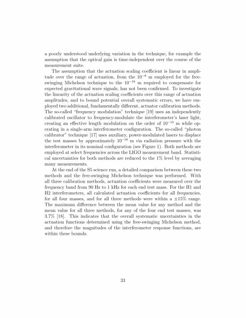
a poorly understood underlying variation in the technique, for example theassumption that the optical gain is time-independent over the course of themeasurement suite.

The assumption that the actuation scaling coefficient is linear in ampli-tude over the range of actuation, from the 10−8 m employed for the free-swinging Michelson technique to the 10−18 m required to compensate forexpected gravitational wave signals, has not been confirmed. To investigatethe linearity of the actuation scaling coefficients over this range of actuationamplitudes, and to bound potential overall systematic errors, we have em-ployed two additional, fundamentally different, actuator calibration methods.The so-called “frequency modulation” technique [19] uses an independentlycalibrated oscillator to frequency-modulate the interferometer’s laser light,creating an effective length modulation on the order of 10−13 m while op-erating in a single-arm interferometer configuration. The so-called “photoncalibrator” technique [17] uses auxiliary, power-modulated lasers to displacethe test masses by approximately 10−18 m via radiation pressure with theinterferometer in its nominal configuration (see Figure 1). Both methods areemployed at select frequencies across the LIGO measurement band. Statisti-cal uncertainties for both methods are reduced to the 1% level by averagingmany measurements.

At the end of the S5 science run, a detailed comparison between these twomethods and the free-swinging Michelson technique was performed. Withall three calibration methods, actuation coefficients were measured over thefrequency band from 90 Hz to 1 kHz for each end test mass. For the H1 andH2 interferometers, all calculated actuation coefficients–for all frequencies,for all four masses, and for all three methods–were within a ±15% range.The maximum difference between the mean value for any method and themean value for all three methods, for any of the four end test masses, was3.7% [18]. This indicates that the overall systematic uncertainties in theactuation functions determined using the free-swinging Michelson method,and therefore the magnitudes of the interferometer response functions, arewithin these bounds.

33

102

103

10!12

10!11

10!10

10!9

S5 H1 Length Response Function

Frequency (Hz)

Ma

gn

itu

de

(m

/ct)

Epoch 1Epoch 2Epoch 3Epoch 4

102

103

!200

!100

0

100

200

Frequency (Hz)

Ph

ase

(d

eg

)

cre

ate

d b

y p

lotS

5re

sp

on

se

fun

ctio

n o

n 2

1!

Ap

r!2

01

0 ,

J.

Kis

se

l

102

103

10!13

10!12

10!11

10!10

S5 H2 Length Response Function

Frequency (Hz)

Magnitude (

m/c

t)

Epoch 1Epoch 2Epoch 3Epoch 4

102

103

!200

!100

0

100

200

Frequency (Hz)

Phase (

deg)

cre

ate

d b

y p

lotS

5re

sponsefu

nction o

n 2

1!

Apr!

2010 , J

. K

issel

102

103

10!13

10!12

10!11

10!10

S5 L1 Length Response Function

Frequency (Hz)

Ma

gn

itu

de

(m

/ct)

Epoch 1Epoch 2Epoch 3

102

103

!200

!100

0

100

200

Frequency (Hz)

Ph

ase

(d

eg

)

cre

ate

d b

y p

lotS

5re

sp

on

se

fun

ctio

n o

n 2

1!

Ap

r!2

01

0 ,

J.

Kis

se

l

Figure 15: Frequency dependent response function, RL(f), for the three LIGO interfer-ometers for all epochs of the S5 science run.

34

102

103

10−2

10−1

S5 H1 Response Function Error BudgetEpoch 3

Mag

nitu

de (

frac

tiona

l err

or)

102

103

10−1

100

101

Pha

se (

deg)

Frequency (Hz)

crea

ted

by C

alcH

1Err

_kis

sel o

n 15

−Ju

n−20

10

102

103

10−2

10−1

S5 H2 Response Function Error BudgetEpoch 3

Mag

nitu

de (

frac

tiona

l err

or)

102

103

10−1

100

101

Pha

se (

deg)

Frequency (Hz)

crea

ted

by C

alcH

2Err

_kis

sel o

n 15

−Ju

n−20

10

102

103

10−2

10−1

S5 L1 Response Function Error BudgetEpoch 3

Mag

nitu

de (

frac

tiona

l err

or)

102

103

10−1

100

101

Pha

se (

deg)

Frequency (Hz)

crea

ted

by C

alcL

1Err

_kis

sel o

n 15

−Ju

n−20

10

102

10!2

10!1

S5 H1 Response Function Error BudgetEpoch 1

Ma

gn

itu

de

(fr

actio

na

l e

rro

r)

!|A|

/|A|

ReW (!|G|

/|G|)

ImW !" G

ReW (!#/#)

HFP

/HSP

Error in G

!|R|

/|R|

102

10!1

100

101

Frequency (Hz)

Ph

ase

(d

eg

)

!" A

ImW (!|G|

/|G|)

ReW !" G

ImW (!#/#)

HFP

/HSP

Error in G

!" R

102

10!2

10!1

S5 H1 Response Function Error BudgetEpoch 1

Ma

gn

itu

de

(fr

actio

na

l e

rro

r)

!|A|

/|A|

ReW (!|G|

/|G|)

ImW !" G

ReW (!#/#)

HFP

/HSP

Error in G

!|R|

/|R|

102

10!1

100

101

Frequency (Hz)

Ph

ase

(d

eg

)

!" A

ImW (!|G|

/|G|)

ReW !" G

ImW (!#/#)

HFP

/HSP

Error in G

!" R

Figure 16: Frequency dependent error estimates for the response function for H1 (topleft), H2 (top right), and L1 (bottom left). In magnitude (top panel) and phase (bottompanel), the total uncertainty (dashed-black) is composed of the uncertainty in actuation,σ|A|/|A|, σφA

(in blue), the open loop transfer function magnitude σ|G|/|G| (in green), theopen loop transfer function phase, σφG

(in red), the time-dependent factor, σγ/γ (in cyan),and from the single pole approximation of the Fabry-Perot cavity response (in magenta).

35

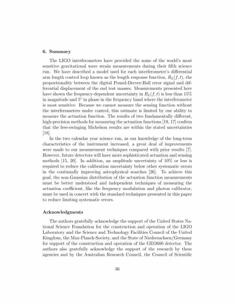
6. Summary

The LIGO interferometers have provided the some of the world’s mostsensitive gravitational wave strain measurements during their fifth sciencerun. We have described a model used for each interferometer’s differentialarm length control loop known as the length response function, RL(f, t), theproportionality between the digital Pound-Drever-Hall error signal and dif-ferential displacement of the end test masses. Measurements presented herehave shown the frequency-dependent uncertainty in RL(f, t) is less than 15%in magnitude and 5 in phase in the frequency band where the interferometeris most sensitive. Because we cannot measure the sensing function withoutthe interferometers under control, this estimate is limited by our ability tomeasure the actuation function. The results of two fundamentally different,high-precision methods for measuring the actuation functions [19, 17] confirmthat the free-swinging Michelson results are within the stated uncertainties[18].

In the two calendar year science run, as our knowledge of the long-termcharacteristics of the instrument increased, a great deal of improvementswere made to our measurement techniques compared with prior results [7].However, future detectors will have more sophisticated actuation and sensingmethods [15, 20]. In addition, an amplitude uncertainty of 10% or less isrequired to reduce the calibration uncertainty below other systematic errorsin the continually improving astrophysical searches [26]. To achieve thisgoal, the non-Gaussian distribution of the actuation function measurementsmust be better understood and independent techniques of measuring theactuation coefficient, like the frequency modulation and photon calibrator,must be used in concert with the standard techniques presented in this paperto reduce limiting systematic errors.

Acknowledgments

The authors gratefully acknowledge the support of the United States Na-tional Science Foundation for the construction and operation of the LIGOLaboratory and the Science and Technology Facilities Council of the UnitedKingdom, the Max-Planck-Society, and the State of Niedersachsen/Germanyfor support of the construction and operation of the GEO600 detector. Theauthors also gratefully acknowledge the support of the research by theseagencies and by the Australian Research Council, the Council of Scientific

36

and Industrial Research of India, the Istituto Nazionale di Fisica Nucle-are of Italy, the Spanish Ministerio de Educacion y Ciencia, the Conselleriad’Economia Hisenda i Innovacio of the Govern de les Illes Balears, the RoyalSociety, the Scottish Funding Council, the Scottish Universities Physics Al-liance, The National Aeronautics and Space Administration, the CarnegieTrust, the Leverhulme Trust, the David and Lucile Packard Foundation, theResearch Corporation, and the Alfred P. Sloan Foundation.

LIGO was constructed by the California Institute of Technology and Mas-sachusetts Institute of Technology with funding from the National ScienceFoundation and operates under cooperative agreement PHY-0107417. Thispaper has LIGO Document Number ligo-p0900120.

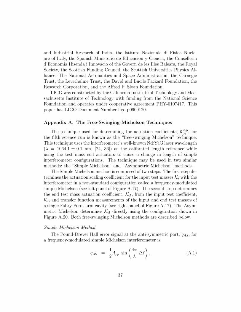
Appendix A. The Free-Swinging Michelson Techniques

The technique used for determining the actuation coefficients, Kx,yA , forthe fifth science run is known as the “free-swinging Michelson” technique.This technique uses the interferometer’s well-known Nd:YaG laser wavelength(λ = 1064.1 ± 0.1 nm, [24, 36]) as the calibrated length reference whileusing the test mass coil actuators to cause a change in length of simpleinterferometer configurations. The technique may be used in two similarmethods: the “Simple Michelson” and “Asymmetric Michelson” methods.

The Simple Michelson method is composed of two steps. The first step de-termines the actuation scaling coefficient for the input test massesKi with theinterferometer in a non-standard configuration called a frequency-modulatedsimple Michelson (see left panel of Figure A.17). The second step determinesthe end test mass actuation coefficient, KA, from the input test coefficient,Ki, and transfer function measurements of the input and end test masses ofa single Fabry Perot arm cavity (see right panel of Figure A.17). The Asym-metric Michelson determines KA directly using the configuration shown inFigure A.20. Both free-swinging Michelson methods are described below.

Simple Michelson Method

The Pound-Drever Hall error signal at the anti-symmetric port, qAS, fora frequency-modulated simple Michelson interferometer is

qAS =1

2App sin

(4π

λ∆`

), (A.1)

37

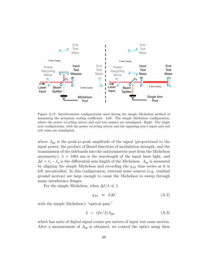
Power

Recycling

Mirror

Beam

Splitter

Input

Test

Masses

X Arm Cavity

Y Arm Cavity

Michelson

Port

Laser

Input

Power

Recycling

Mirror

Beam

Splitter

End

Test

Mass

X Arm Cavity

Y Arm Cavity

Single Arm

Port

Laser

Input

Input

Test

Mass

End

Test

Mass

End

Test

Mass

End

Test

Mass

Figure A.17: Interferometer configurations used during the simple Michelson method ofmeasuring the actuation scaling coefficient. Left: The simple Michelson configuration,where the power recycling mirror and end test masses are misaligned. Right: The singlearm configuration, with the power recycling mirror and the opposing arm’s input and endtest mass are misaligned.

where App is the peak-to-peak amplitude of the signal (proportional to theinput power, the product of Bessel functions of modulation strength, and thetransmission of the sidebands into the antisymmetric port from the Michelsonasymmetry), λ = 1064 nm is the wavelength of the input laser light, and∆` = `x− `y is the differential arm length of the Michelson. App is measuredby aligning the simple Michelson and recording the qAS time series as it isleft uncontrolled. In this configuration, external noise sources (e.g. residualground motion) are large enough to cause the Michelson to sweep throughmany interference fringes.

For the simple Michelson, when ∆`/λ 1,

qAS ≈ k∆` (A.2)

with the simple Michelson’s “optical gain,”

k = (2π/λ)App, (A.3)

which has units of digital signal counts per meters of input test mass motion.After a measurement of App is obtained, we control the optics using their

38

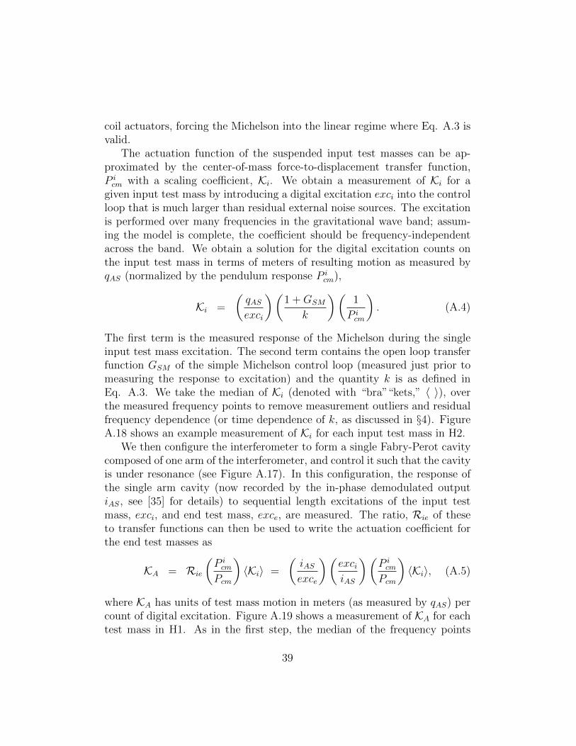
coil actuators, forcing the Michelson into the linear regime where Eq. A.3 isvalid.

The actuation function of the suspended input test masses can be ap-proximated by the center-of-mass force-to-displacement transfer function,P icm with a scaling coefficient, Ki. We obtain a measurement of Ki for a

given input test mass by introducing a digital excitation exci into the controlloop that is much larger than residual external noise sources. The excitationis performed over many frequencies in the gravitational wave band; assum-ing the model is complete, the coefficient should be frequency-independentacross the band. We obtain a solution for the digital excitation counts onthe input test mass in terms of meters of resulting motion as measured byqAS (normalized by the pendulum response P i

cm),

Ki =

(qASexci

)(1 +GSM

k

)(1

P icm

). (A.4)

The first term is the measured response of the Michelson during the singleinput test mass excitation. The second term contains the open loop transferfunction GSM of the simple Michelson control loop (measured just prior tomeasuring the response to excitation) and the quantity k is as defined inEq. A.3. We take the median of Ki (denoted with “bra”“kets,” 〈 〉), overthe measured frequency points to remove measurement outliers and residualfrequency dependence (or time dependence of k, as discussed in §4). FigureA.18 shows an example measurement of Ki for each input test mass in H2.

We then configure the interferometer to form a single Fabry-Perot cavitycomposed of one arm of the interferometer, and control it such that the cavityis under resonance (see Figure A.17). In this configuration, the response ofthe single arm cavity (now recorded by the in-phase demodulated outputiAS, see [35] for details) to sequential length excitations of the input testmass, exci, and end test mass, exce, are measured. The ratio, Rie of theseto transfer functions can then be used to write the actuation coefficient forthe end test masses as

KA = Rie

(P icm

Pcm

)〈Ki〉 =

(iASexce

)(exciiAS

)(P icm

Pcm

)〈Ki〉, (A.5)

where KA has units of test mass motion in meters (as measured by qAS) percount of digital excitation. Figure A.19 shows a measurement of KA for eachtest mass in H1. As in the first step, the median of the frequency points

39

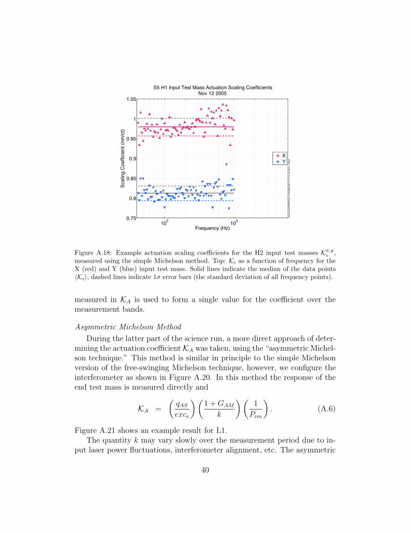
102

103

0.75

0.8

0.85

0.9

0.95

1

1.05

S5 H1 Input Test Mass Actuation Scaling CoefficientsNov 12 2005

Frequency (Hz)

Scalin

g C

oeffic

ient (n

m/c

t)

cre

ate

d b

y p

lotE

TM

DC

Ca

ls_

H1

Sim

pM

ich

05

11

12

on

15!

Ju

l!2

01

0 ,

J.

Kis

se

l

XY

Figure A.18: Example actuation scaling coefficients for the H2 input test masses Kx,yi ,measured using the simple Michelson method. Top: Ki as a function of frequency for theX (red) and Y (blue) input test mass. Solid lines indicate the median of the data points〈Ki〉, dashed lines indicate 1σ error bars (the standard deviation of all frequency points).

measured in KA is used to form a single value for the coefficient over themeasurement bands.

Asymmetric Michelson Method

During the latter part of the science run, a more direct approach of deter-mining the actuation coefficientKA was taken, using the “asymmetric Michel-son technique.” This method is similar in principle to the simple Michelsonversion of the free-swinging Michelson technique, however, we configure theinterferometer as shown in Figure A.20. In this method the response of theend test mass is measured directly and

KA =

(qASexce

)(1 +GAM

k

)(1

Pcm

). (A.6)

Figure A.21 shows an example result for L1.The quantity k may vary slowly over the measurement period due to in-

put laser power fluctuations, interferometer alignment, etc. The asymmetric

40

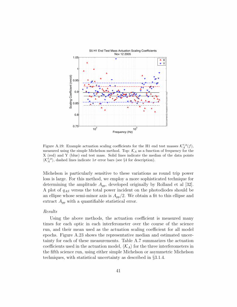
102

103

0.75

0.8

0.85

0.9

0.95

1

1.05

S5 H1 End Test Mass Actuation Scaling CoefficientsNov 12 2005

Frequency (Hz)

Scalin

g C

oeffic

ient (n

m/c

t)

cre

ate

d b

y p

lotE

TM

DC

Cals

_H

1S

impM

ich051112 o

n 1

5!

Jul!

2010 , J

. K

issel

XY

Figure A.19: Example actuation scaling coefficients for the H1 end test masses Kx,yA (f),measured using the simple Michelson method. Top: KA as a function of frequency for theX (red) and Y (blue) end test mass. Solid lines indicate the median of the data points〈Kx,yA 〉, dashed lines indicate 1σ error bars (see §4 for description).

Michelson is particularly sensitive to these variations as round trip powerloss is large. For this method, we employ a more sophisticated technique fordetermining the amplitude App, developed originally by Rolland et al [32].A plot of qAS versus the total power incident on the photodiodes should bean ellipse whose semi-minor axis is App/2. We obtain a fit to this ellipse andextract App with a quantifiable statistical error.

Results

Using the above methods, the actuation coefficient is measured manytimes for each optic in each interferometer over the course of the sciencerun, and their mean used as the actuation scaling coefficient for all modelepochs. Figure A.23 shows the representative median and estimated uncer-tainty for each of these measurements. Table A.7 summarizes the actuationcoefficients used in the actuation model, 〈KA〉 for the three interferometers inthe fifth science run, using either simple Michelson or asymmetric Michelsontechniques, with statistical uncertainty as described in §3.1.4.

41

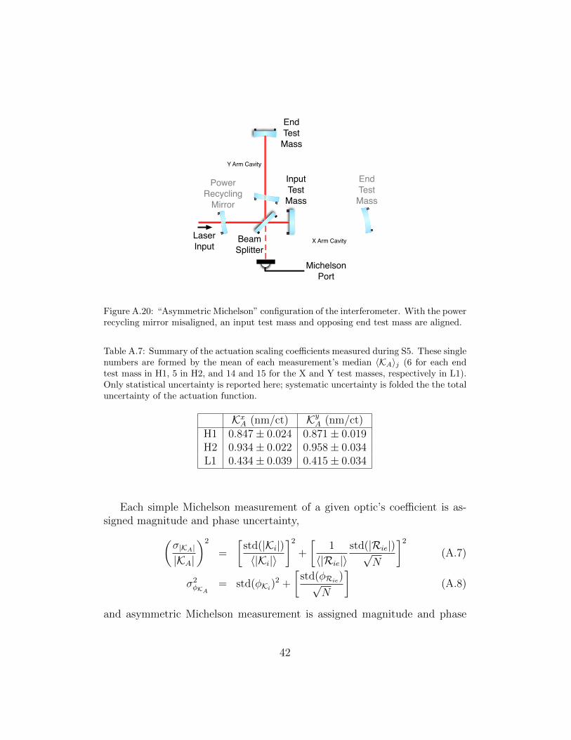
Power

Recycling

Mirror

Beam

Splitter

Input

Test

Mass

End

Test

Mass

X Arm Cavity

Y Arm Cavity

Michelson

Port

End

Test

Mass

Laser

Input

Figure A.20: “Asymmetric Michelson” configuration of the interferometer. With the powerrecycling mirror misaligned, an input test mass and opposing end test mass are aligned.

Table A.7: Summary of the actuation scaling coefficients measured during S5. These singlenumbers are formed by the mean of each measurement’s median 〈KA〉j (6 for each endtest mass in H1, 5 in H2, and 14 and 15 for the X and Y test masses, respectively in L1).Only statistical uncertainty is reported here; systematic uncertainty is folded the the totaluncertainty of the actuation function.

KxA (nm/ct) KyA (nm/ct)H1 0.847± 0.024 0.871± 0.019H2 0.934± 0.022 0.958± 0.034L1 0.434± 0.039 0.415± 0.034

Each simple Michelson measurement of a given optic’s coefficient is as-signed magnitude and phase uncertainty,(

σ|KA|

|KA|

)2

=

[std(|Ki|)〈|Ki|〉

]2

+

[1

〈|Rie|〉std(|Rie|)√

N

]2

(A.7)

σ2φKA

= std(φKi)2 +

[std(φRie

)√N

](A.8)

and asymmetric Michelson measurement is assigned magnitude and phase

42

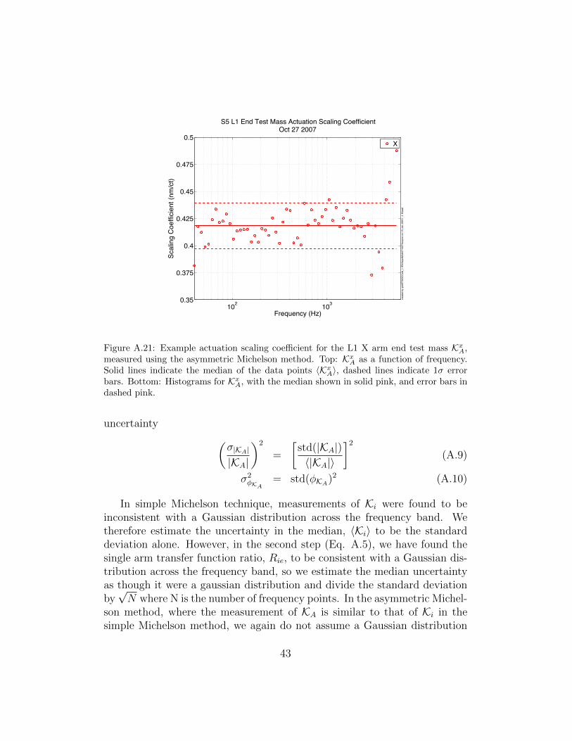
102

103

0.35

0.375

0.4

0.425

0.45

0.475

0.5

S5 L1 End Test Mass Actuation Scaling CoefficientOct 27 2007

Frequency (Hz)

Scalin

g C

oeffic

ient (n

m/c

t)

cre

ate

d b

y p

lotE

TM

DC

Cals

_L1E

XA

sym

Mic

h071027A

cquire o

n 1

5!

Jul!

2010 , J

. K

issel

X

Figure A.21: Example actuation scaling coefficient for the L1 X arm end test mass KxA,measured using the asymmetric Michelson method. Top: KxA as a function of frequency.Solid lines indicate the median of the data points 〈KxA〉, dashed lines indicate 1σ errorbars. Bottom: Histograms for KxA, with the median shown in solid pink, and error bars indashed pink.

uncertainty (σ|KA|

|KA|

)2

=

[std(|KA|)〈|KA|〉

]2

(A.9)

σ2φKA

= std(φKA)2 (A.10)

In simple Michelson technique, measurements of Ki were found to beinconsistent with a Gaussian distribution across the frequency band. Wetherefore estimate the uncertainty in the median, 〈Ki〉 to be the standarddeviation alone. However, in the second step (Eq. A.5), we have found thesingle arm transfer function ratio, Rie, to be consistent with a Gaussian dis-tribution across the frequency band, so we estimate the median uncertaintyas though it were a gaussian distribution and divide the standard deviationby√N where N is the number of frequency points. In the asymmetric Michel-

son method, where the measurement of KA is similar to that of Ki in thesimple Michelson method, we again do not assume a Gaussian distribution

43

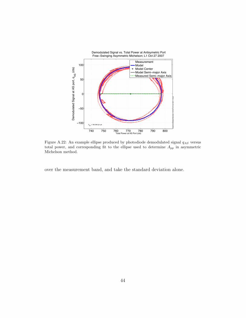
740 750 760 770 780 790 800

!100

!50

0

50

100

Demodulated Signal vs. Total Power at Antisymetric PortFree!Swinging Asymmetric Michelson; L1 Oct 27 2007

Total Power at AS Port (cts)

Dem

odula

ted S

ignal at A

S p

ort

, q

AS (

cts

)

App

= 184.384 pk!pk

cre

ate

d b

y p

lotE

llip

se

FitE

xam

ple

_L

10

710

27

on

15!

Jul!

2010

, J

. K

issel

MeasurementModelModel CenterModel Semi!major AxisMeasured Semi!major Axis

Figure A.22: An example ellipse produced by photodiode demodulated signal qAS versustotal power, and corresponding fit to the ellipse used to determine App in asymmetricMichelson method.

over the measurement band, and take the standard deviation alone.

44

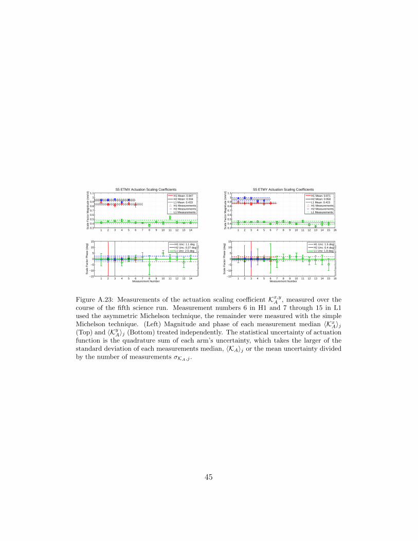
1 2 3 4 5 6 7 8 9 10 11 12 13 140.3

0.4

0.5

0.6

0.7

0.8

0.9

1

1.1S5 ETMX Actuation Scaling Coefficients

Sca

le F

acto

r M

agni

tude

(nm

/ct)

1 2 3 4 5 6 7 8 9 10 11 12 13 14−15

−10

−5

0

5

10

15

Measurement Number

Sca

le F

acto

r P

hase

(de

g)

crea

ted

by m

akeb

inne

dact

erro

r on

15−

Jul−

2010

, J.

Kis

sel

H1 Mean: 0.847H2 Mean: 0.934L1 Mean: 0.433H1 MeasurementsH2 MeasurementsL1 Measurements

H1 Unc: 1.1 degH2 Unc: 0.27 degL1 Unc: 2.5 deg

1 2 3 4 5 6 7 8 9 10 11 12 13 14 15 160.3

0.4

0.5

0.6

0.7

0.8

0.9

1

1.1S5 ETMY Actuation Scaling Coefficients

Sca

le F

acto

r M

agni

tude

(nm

/ct)

1 2 3 4 5 6 7 8 9 10 11 12 13 14 15 16−15

−10

−5

0

5

10

15

Measurement Number

Sca

le F

acto

r P

hase

(de

g)

crea

ted

by m

akeb

inne

dact

erro

r on

15−

Jul−

2010

, J.

Kis

sel

H1 Mean: 0.871H2 Mean: 0.958L1 Mean: 0.415H1 MeasurementsH2 MeasurementsL1 Measurements

H1 Unc: 1.5 degH2 Unc: 0.4 degL1 Unc: 1.8 deg

Figure A.23: Measurements of the actuation scaling coefficient Kx,yA , measured over thecourse of the fifth science run. Measurement numbers 6 in H1 and 7 through 15 in L1used the asymmetric Michelson technique, the remainder were measured with the simpleMichelson technique. (Left) Magnitude and phase of each measurement median 〈KxA〉j(Top) and 〈KyA〉j (Bottom) treated independently. The statistical uncertainty of actuationfunction is the quadrature sum of each arm’s uncertainty, which takes the larger of thestandard deviation of each measurements median, 〈KA〉j or the mean uncertainty dividedby the number of measurements σKA,j .

45

References

[1] Abbott, B. P., et al., 2009. Einstein@home search for periodic gravita-tional waves in early S5 LIGO data. Phys. Rev. D 80 (042003).

[2] Abbott, B. P., et al., 2009. LIGO: The laser interferometer gravitational-wave observatory. Rep. Prog. Phys. 72 (076901).

[3] Abbott, B. P., et al., 2009. Search for high-frequency gravitational wavebursts in the first calendar year of LIGO’s fifth science run. Phys. Rev.D 80 (102002).

[4] Abbott, B. P., et al., 2009. Sensitivity to gravitational waves from com-pact binary coalescences achieved during LIGO’s fifth and VIRGO’s firstscience run. LIGO Internal Document, T0900499. <https://dcc.ligo.org/cgi-bin/DocDB/DocumentDatabase/>.

[5] Abbott, B. P., et al., 2009. An upper limit on the stochasticgravitational-wave background of cosmological origin. Nature 460 (990).

[6] Abramovici, A., et al., 1992. LIGO: The laser interferometergravitational-wave observatory. Science 17 (256).

[7] Adhikari, R., Gonzalez, G., Landry, M., O’Reilly, B., 2003. Calibrationof the LIGO detectors for the first LIGO science run. Class. QuantumGrav. 20 (17).

[8] Anderson, W., Brady, P. R., Chin, D., Creighton, J. D. E., Riles, K.,Whelan, J. T., 2001. Beam pattern response functions and times of ar-rival for earthbound interferometer. LIGO Internal Document, T010110.<https://dcc.ligo.org/cgi-bin/DocDB/DocumentDatabase/>.

[9] Anderson, W. G., Brady, P. R., Creighton, J. D. E., Flanagan, E. E.,2001. Excess power statistic for detection of burst sources of gravita-tional radiation. Phys. Rev. D 63 (042003).

[10] Aso, Y., et al., 2009. Accurate measurement of the time delay in the re-sponse of the LIGO gravitational wave detectors. Class. Quantum Grav.26 (055010).

[11] Christi, R., 2004. Modern Digital Signal Processing. Brooks/Cole.

46

[12] Coyne, D., 1998. Test mass transmissibility. LIGO InternalDocument, T970191. <https://dcc.ligo.org/cgi-bin/DocDB/

DocumentDatabase/>.

[13] Drever, R., Hall, J., Kowalski, F., Hough, J., Ford, G., Munley, A.,Ward, H., 1983. Laser phase and frequency stabilization using an opticalresonator. Applied Physics B: Lasers Opt. 31 (97-105).

[14] Evans, M., Mavalvala, N., Fritschel, P., Bork, R., Bhawal, B., Gustafson,R., Kells, W., Landry, M., Sigg, D., Weiss, R., Whitcomb, S., Ya-mamoto., H., 2002. Lock acquisition of a gravitational-wave interfer-ometer. Opt. Lett. 27 (8).

[15] Fritschel, P., 2003. Second generation instruments for the laser inter-ferometer gravitational wave observatory (LIGO). Proceedings of SPIE4856, arXiv:gr-qc/0308090v1.

[16] Fritschel, P., Bork, R., Gonzlez, G., Mavalvala, N., Ouimette, D., Rong,H., Sigg, D., Zucker, M., 2001. Readout and control of a power-recycledinterferometric gravitational wave antenna. Appl. Opt. 40 (4988).

[17] Goetz, E., et al, 2009. Precise calibration of LIGO test mass actuatorsusing photon radiation pressure. Class. Quantum Grav. 26 (245011).

[18] Goetz, E., et al., 2010. Accurate calibration of test mass displacementin the LIGO interferometers. Class. Quantum Grav. 27 (084024).

[19] Goetz, E., Savage Jr., R. L., 2009. Calibration of the LIGO displace-ment actuators via laser frequency modulation. Class. Quantum Grav.arXiv:1005.3746v1.

[20] Harry, G., 2009. Advanced LIGO: the next generation of gravitationalwave detectors. Class. Quantum Grav. 27 (084006).

[21] Hawking, S. W., Israel, W. (Eds.), 1987. Three hundred years of gravi-tation. Cambridge University Press, Ch. 6, pp. 330 – 446.

[22] Kawabe, K., O’Reilly, B., Siemens, X., 2010. Summary of s5 calibrationmodels and uncertainties. LIGO Internal Document, T1000227. <https://dcc.ligo.org/cgi-bin/DocDB/DocumentDatabase/>.

47

[23] Kissel, J. S., 2009. Uncertainty estimation of the LIGO response func-tion. LIGO Internal Document, T0900555. <https://dcc.ligo.org/

cgi-bin/DocDB/DocumentDatabase/>.

[24] Koechner, K., 1992. Solid-State Later Engineering, 3rd Edition.Springer-Verlag.

[25] Landry, M., 2005. LIGO test mass mechanical resonances. LIGO In-ternal Document. T050089. <https://dcc.ligo.org/cgi-bin/DocDB/DocumentDatabase/>.

[26] Lindblom, L., 2009. Optimal calibration accuracy for gravitational wavedetectors. Phys. Rev. D 80 (042005).

[27] Morse, P. M., Ingard, K. U., 1986. Theoretical Acoustics. PrincetonUniversity Press.

[28] Oppenheim, A. V., Schafer, R. W., 1975. Digital Signal Processing.Prentice-Hall.

[29] Rakhmanov, M., Romano, J. D., Whelan, J. T., 2008. High-frequencycorrections to the detector response and their effect on searches for grav-itational waves. Class. Quantum Grav. 25 (184017).

[30] Rakhmanov, M., Savage, R., Reitze, D., Tanner, D., 2002. Dynamicresonance of light in Fabry-Perot cavities. Physics Letters A 305.

[31] Regehr, M., Raab, F., Whitcomb, S., 1995. Demonstration of a power re-cycled Michelson interferometer with Fabry-Perot arms by frontal mod-ulation. Opt. Lett. 20 (1507-1509).

[32] Rolland, L., et al., 2007. VIRGO actuator gain calibration : methodsand results. Period September 2006 to April 2007. VIRGO Internal Doc-ument, VIR-0005A-07. <https://pub3.ego-gw.it/itf/tds/>.

[33] Siemens, X., et al., 2004. Making h(t) for LIGO. Class. Quantum Grav.21 (S1723).

[34] Sigg, D., 1997. Strain calibration of LIGO. LIGO Internal Document,T970101. <http://admdbsrv.ligo.caltech.edu/dcc/>.

48

[35] Sigg, D., et al., 1997. Frequency response of the LIGO interferom-eter. LIGO Internal Document, T970084. <http://admdbsrv.ligo.

caltech.edu/dcc/>.

[36] Singh, S., Smith, R. G., Uitert, L. G. V., 1974. Stimulated-emission crosssection and fluorescent quantum efficiency of Nd3+ in yttrium aluminumgarnet at room temperature. Phys. Rev. B 10 (2566-2572).

[37] Thorne, K. S., 1997. Gravitational radiation a new window onto theuniverse. Class. Quantum Grav. arXiv:gr-qc/9704042v1.

49