arX

iv:g

r-qc

/950

7035

v1 1

4 Ju

l 199

5

Wave Propagation in Gravitational Systems:

Late Time Behavior

E.S.C. Ching(1), P.T. Leung(1), W.M. Suen(2), and K. Young(1)

(1)Department of Physics, The Chinese University of Hong Kong, Hong Kong

(2)Department of Physics, Washington University, St Louis, MO 63130, U S A

(March 22, 1995)

Abstract

It is well-known that the dominant late time behavior of waves propagating

on a Schwarzschild spacetime is a power-law tail; tails for other spacetimes

have also been studied. This paper presents a systematic treatment of the tail

phenomenon for a broad class of models via a Green’s function formalism and

establishes the following. (i) The tail is governed by a cut of the frequency

Green’s function G(ω) along the − Im ω axis, generalizing the Schwarzschild

result. (ii) The ω dependence of the cut is determined by the asymptotic

but not the local structure of space. In particular it is independent of the

presence of a horizon, and has the same form for the case of a star as well. (iii)

Depending on the spatial asymptotics, the late time decay is not necessarily a

power law in time. The Schwarzschild case with a power-law tail is exceptional

among the class of the potentials having a logarithmic spatial dependence.

(iv) Both the amplitude and the time dependence of the tail for a broad class

of models are obtained analytically. (v) The analytical results are in perfect

agreement with numerical calculations.

PACS numbers: 04.30.-w

Typeset using REVTEX

1

I. INTRODUCTION

In this paper we are concerned with the systematics of the propagation of linearized

waves on curved background, in particular, the late time behavior [1]. The problem is of

interest for understanding wave phenomena in relativity [2–6], and possibly in other areas

of physics. The propagation of linearized gravitational, electromagnetic and scalar waves is

often modeled by the Klein-Gordon (KG) equation with an effective potential

Dφ(x, t) ≡[∂2

t − ∂2x + V (x)

]φ(x, t) = 0, (1.1)

which includes the Zerilli and Regge-Wheeler equations as special examples [7]. The effective

potential V (x) describes the scattering of φ by the background curvature. We are here

interested in the evolution of φ in the presence of this scattering.

On flat space (V = 0), waves travel along the light cone: φ(x, t) = φ+(x− t)+φ−(x+ t),

but the situation is much more interesting in the presence of a nontrivial background. Fig. 1

shows the result of a typical numerical experiment evolving (1.1) on 0 ≤ x < ∞ (so that

x may be thought of as a radial variable, see below), with the boundary condition φ(x =

0, t) = 0, and the condition of outgoing waves for x → ∞. An initial gaussian φ centered

at yo with initial φ = 0 is allowed to evolve, and is observed at x1 > yo. The figure shows

φ(x1, t) versus t. Our interest in this paper is the behavior at large t, but it is useful to first

place the time dependence in an overall context.

The generic time dependence of waves observed at a fixed spatial location x1 consists of

three components, as illustrated in Fig. 1. (i) The prompt contribution (peaks A and C in

Fig. 1a) depends strongly on the initial conditions. The first peak A is due to the initial

pulse propagating from yo directly to the right, while the later peak C is due to the initial

pulse propagating from yo to the left, being reflected and inverted at the origin, and then

propagating to the observation point x1. (ii) Each of these pulses is followed by a trailing

signal (respectively B and D) caused by the potential V (in the sense that B and D vanish

when V = 0). The latter pulse D has traversed regions of larger V , and as a result is both

2

more pronounced in amplitude and also more compressed in time. On a longer time scale

(Fig. 1b), it is seen that scattering by the potential (e.g. peak D) merges into a train of

quasinormal ringing, decaying in an exponential manner. (iii) Finally, there is a tail, which

decays approximately as a power in t (a straight line in this log-log plot), and it dominates

at late times.

The prompt contribution is most intuitive, being the obvious counterpart of the light-

cone propagation in the V = 0 case, and is in any event expected in the semi-classical limit.

The ringing is due to a superposition of quasinormal modes [which are solutions to (1.1) with

the time dependence e−iωt for some complex ω]. These are particularly interesting in that

the time dependence (both of the quasinormal modes and of the trailing signals B and D)

observed far away carries information about the structure of the intervening space. In the

mathematical sense, this is because the quasinormal mode frequencies ω are determined by

V (x). In a more physical sense, it is useful to consider the analogy of electromagnetic waves

emitted by a source in an optical cavity; the cavity, in providing a nontrivial environment,

is analogous to the presence of a potential V (x) in (1.1). [In fact, a one-dimensional scalar

model of electromagnetic waves would be described by a wave equation with a nontrivial

dielectric constant distribution n2(x) [8]; such a wave equation would be very similar to

(1.1) and in fact can be transformed into it [9].] For a broad band source in a laser cavity

of length L, the spectrum of electromagnetic waves observed far away would have frequency

components ω ≈ jπc/L, where j is an integer. In this sense, these quasinormal modes carry

information about the cavity. In much the same way, the ringing component of the solution

in (1.1), if observed, would carry significant information about the background curvature of

the intervening space. For this reason, there have been extensive numerical studies of various

models. In addition, one particularly intriguing possibility is that the sum of quasinormal

modes may be complete in a certain sense, as the normal modes of a conservative system

are complete. If this were the case, one would have a discrete spectral representation of the

dynamics, with obvious conceptual and computational advantages. The completeness has

been demonstrated in the analogous case of the wave equation [10], and its generalization

3

to the KG equation (1.1) will be reported elsewhere [11].

This paper develops a general treatment for the late time behavior of a field satisfying

(1.1) with a broad class of time-independent potentials V (x) and the outgoing wave boundary

condition. Such a system could describe linearized waves evolving in stationary spacetimes

with or without horizons, and in vacuum or nonvacuum spacetimes. For example, for a

general static spherically symmetric spacetime,

ds2 = gtt(r)dt2 + grr(r)dr

2 + r2(dθ2 + sin2 θdϕ2) , (1.2)

a Klein-Gordon scalar field Φ can be expressed as

Φ =∑

lm

1

rφlm(x, t)Ylm(θ, ϕ). (1.3)

The evolution of φlm(x, t) is given by (1.1) with the effective potential

V (x) = −gttl(l + 1)

r2− 1

2r

gtt

grr

[∂rgtt

gtt− ∂rgrr

grr

], (1.4)

where x is related to the circumferential radius r by

x =∫ √

−grr

gttdr (1.5)

and extends over a half-line if the metric is non-singular, but extends over the full line when

there is a horizon.

The special case of linearized perturbations of a black hole background has received much

attention [4–7,12,13]. In the simplest case of the Schwarzschild spacetime

ds2 = −(1 − 2M

r

)dt2 +

(1 − 2M

r

)−1

dr2 + r2(dθ2 + sin2 θdϕ2) , (1.6)

the transformation (1.5) leads to

x = r + 2M log(r

2M− 1

). (1.7)

For a Klein-Gordon scalar field, V is defined by (1.4) and takes the explicit form

V (x) =(1 − 2M

r

) [l(l + 1)

r2+ (1 − S2)

2M

r3

], (1.8)

4

with S = 0. Electromagnetic and gravitational waves also obey (1.1) and (1.8), but with

S = 1, 2 respectively [7]. The boundary condition is outgoing waves at r = 2M (x → −∞,

into the black hole) and as r → ∞ (x → ∞). With the effective potential (1.8), it is

well known that the tail decays as t−(2l+3) independent of the spin S of the field [4]. For

Reissner-Nordstrom black holes, the evolution equation can again be put in form of (1.1),

but with an effective potential slightly different from (1.8). The tail is again found to decay

as t−(2l+3) [5]. Although a similar tail should exist for Kerr black holes, we are not aware of

the corresponding analysis in that case. Most of these previous analyses (except Ref. 3) are

specific to a particular form of the potential.

Several recent developments make a more general study of the late time tail phenomenon

of gravitational systems particularly interesting. As studies of the Schwarzschild spacetime

show that the tail comes from scattering at large radius [4], it has been suggested [5] that

a power-law tail would develop even when there is no horizon in the background, implying

that such tails should be present in perturbations of stars, or after the collapse of a massless

field which does not result in black hole formation. In Ref. 6, the late time behavior of

scalar waves evolving in their own gravitational field or in gravitational fields generated by

other scalar field sources was studied numerically, and power-law tails have been reported

(though with exponents different from the Schwarzchild case). These interesting results call

for a systematic analysis of the tail phenomenon in (i) nonvacuum, (ii) time-dependent, and

(iii) nonlinear spacetimes, for which the present work will lay a useful foundation.

In Section II, we formulate the problem in terms of the Green’s function, leading to a

precise definition of the prompt, quasinormal mode and tail components in terms of con-

tributions from different parts of the complex frequency plane. In Section III, numerical

experiments are presented. The analytic treatment is then given in Section IV (potentials

decreasing faster than x−2), Section V (inverse square potentials) and Section VI (composite

potentials consisting of a centrifugal barrier plus a subsidiary term). The last case, though

technically most complicated, is also the most interesting physically, since it includes, for

example, the potential in (1.8). Section VII contains a discussion and the conclusion.

5

The highlights of this paper are as follows. Firstly, the analytic results agree perfectly

with the numerical experiments, including both the time dependence and the magnitude;

this agreement indicates that the phenomenon of the late time tail has now been quite fully

understood for a large class of models. Secondly, our work extends, places in context, and

provides insight into the known results for the Schwarzschild case. For the Schwarzschild

spacetime, the late time tail has previously been related to either reflection from the asymp-

totic region of the potential [4], or to the Green’s function having a branch cut along the

negative imaginary axis in the complex frequency plane [13]. In this paper, we demon-

strate that the cut is a general feature, if V (x) asymptotically (x → ∞) tends to zero

less rapidly than an exponential, except for the particular case of the “centrifugal barrier”

V (x) = l(l + 1)/x2, l = 1, 2.... Furthermore, we determine the strength of the cut in terms

of the asymptotic form of the potential for a broad class of potentials. These results then

relate the two different explanations of the late time tail in the literature.

Some specific late time behavior we discovered in this paper are of particular interest.

Potentials going as a centrifugal barrier of angular momentum l (l is an integer) plus ∼

x−α(log x)β (β = 0, 1) are of interest, because these include the Schwarzschild case (α =

3, β = 1). For such potentials, the generic late time behavior is ∼ t−(2l+α)(log t)β. Thus, for

β = 1, the late time tail is not a simple power law, but exhibits an additional log t factor.

However, when α is an odd integer less than 2l + 3, the generic leading behavior vanishes.

For β = 0, the next leading term is expected to be t−(2l+2α−2), while for β = 1, the next

leading term is t−(2l+α) without a log t factor. Interestingly, the well-known Schwarzschild

spacetime belongs to such exceptions.

As a collorary, we establish that the form of the late time tail is independent of the

potential at finite x. In particular, whether the background metric describes a star (so that

x is itself the radial variable 0 ≤ x < ∞), or a black hole [so that x is the variable defined

in (1.5), −∞ < x < ∞], the late time tail is the same as long as the asymptotic potential

V (x→ ∞) is the same, thus confirming the suggestion of Ref. 5.

As a by-product, we point out that numerical calculations are sometimes plagued by a

6

“ghost” potential arising out of spatial discretization. The effects of this “ghost” potential

may in some cases mask the genuine tail behavior — which is often numerically very small

(see Fig. 1b). This problem could have led to errors, or at least ambiguities, in some

numerical studies, in particular numerical studies of tail phenomena. This subtlety with

numerical calculations is discussed in Appendix A.

II. FORMALISM

The time evolution of a field φ(x, t) described by (1.1) with given initial data can be

written as [14]

φ(x, t) =∫dy G(x, y; t) ∂tφ(y, 0) +

∫dy ∂tG(x, y; t) φ(y, 0) (2.1)

for t > 0, where the retarded Green’s function G is defined by

DG(x, y; t) = δ(t)δ(x− y) , (2.2)

and the initial condition G(x, y; t) = 0 for t < 0. The Fourier transform

G(x, y;ω) =∫ ∞

0dtG(x, y; t)eiωt (2.3)

satisfies

D(ω)G ≡[−ω2 − ∂2

x + V (x)]G(x, y;ω) = δ(x− y) (2.4)

and is analytic in the upper half ω plane.

Waves propagating on curved space and observed by a distant observer should satisfy

the outgoing wave condition. In terms of this, there are two classes of systems.

(a) For non-singular systems, e.g., an oscillating relativistic star generating gravitational

waves, the variable x, as defined by (1.5), is the radial variable of a three-dimensional

problem, 0 ≤ x <∞. The left boundary condition is taken to be

φ(x = 0, ω) = 0 , (2.5a)

7

while the right boundary condition is one of outgoing waves

φ(x, ω) ∝ eiωx , x→ +∞ , (2.5b)

where φ is the wavefunction in the frequency domain.

(b) For the case of black holes, x given by (1.5) is a full line variable, −∞ < x <∞, where

the left boundary x→ −∞ is the event horizon. We have outgoing waves at both ends, i.e.,

φ(x, ω) ∝ e−iωx , x→ −∞ , (2.6)

together with (2.5b).

For simplicity, we shall write the formalism in terms of the half-line problem, and indicate

briefly the simple changes necessary for the full-line case. We shall assume V → 0 as

|x| → ∞.

Define two auxiliary functions f(ω, x) and g(ω, x) as solutions to the homogeneous equa-

tion D(ω)f(ω, x) = D(ω)g(ω, x) = 0, where f satisfies the left boundary condition and g

satisfies the right boundary condition. To be definite, we adopt the following normalization

conventions:

limx→∞

[e−iωxg(ω, x)] = 1; (2.7)

and for the half-line problem f(ω, x = 0) = 0, f ′(ω, x = 0) = 1 [15], while for the full-line

problem limx→−∞[eiωxf(ω, x)] = 1. Let the Wronskian be W (ω) = W (g, f) = g∂xf − f∂xg,

which is independent of x. It is then straightforward to see that

G(x, y;ω) =

f(ω, x)g(ω, y)W (ω)

, x < y

f(ω, y)g(ω, x)W (ω)

, y < x

. (2.8)

The essence of the problem is, in one guise or another, how to integrate f from the left and g

from the right, until they can be compared at a common value of x, at which the Wronskian

can then be evaluated. The above choice of normalization is for convenience only, since a

8

change of normalization, f → Af and g → Bg, would result in W → ABW with no effect

on G.

Consider the inverse transform of (2.3), and for t > 0 attempt to close the contour in ω

by a semicircle of radius C in the lower half-plane, where eventually one anticipates taking

C → ∞. One is then led to consider the singularities of G for Im ω < 0 (Fig. 2), from which

different contributions to G can be identified as follows.

(a) Tail contribution If the potential V (x) has a finite range, say V (x) = 0 for x > a,

then one can impose the condition (2.7) at x = a+, and integrate the equation through a

finite distance to obtain g(ω, x) for all x < a. Such an integration over a finite range using

an ordinary differential equation cannot lead to any singularity in ω [16]. It is not surprising

that if V (x) does not have finite support, but nevertheless vanishes sufficiently rapidly as

x → +∞, g(ω, x) is still regular. The necessary condition is that V (x) must vanish faster

than any exponential [17], and this is shown in Section IV. However, if V (x) has a tail that

does not decrease rapidly enough, then g(ω, x) will have singularities in ω. A tail that is

exponential at large x, V (x) ∼ e−λx, would in general lead to singularities in g(ω, x) for

− Im ω ≥ λ/2. In so far as these singularities stay away from ω = 0, they have no effect on

the late time behavior. However, if V (x → ∞) ∼ x−α(log x)β (β = 0, 1), then g(ω, x) will

have singularities that lie on the − Im ω axis, and take the form of a branch cut going all

the way to the origin [17], as in the Schwarzschild case [13]. This contribution to G will be

denoted as GL. It is the purpose of this paper to evaluate GL for a broad class of V (x).

For the half-line problem, f(ω, x) is integrated from x = 0 through a finite distance, and

hence does not have any singularities in ω. For the full-line problem, f(ω, x) is dealt with

in the same manner. In all cases of physical interest, V (x) vanishes on the left either faster

than an exponential, or precisely as an exponential [e.g. Schwarzschild spacetime under the

transformation (1.5)]. For the former, f(ω, x) has no singularities in ω, while for the latter,

there will be a series of poles, but at a finite distance from ω = 0. In both cases, there is no

contribution to the late time behavior.

(b) Quasinormal modes Secondly, the Wronskian W (ω) may have zeros at ω = ωj, j =

9

±1,±2, . . ., on the complex ω plane [18]. At these frequencies, f and g are linearly depen-

dent, i.e., one can find a solution that satisfies both the left and the right boundary condition.

Such solutions are by definition quasinormal modes (QNM’s). The collective contribution

of the QNM’s is denoted as GQ(x, y; t). In the case of a Schwarzschild black hole, GQ

has been evaluated semi-analytically by using the phase-integral method [19]. Since each

Im ωj < 0, GQ decays exponentially as t→ ∞, and is, therefore, irrelevant for the late time

behavior. In some cases, GQ(x, y; t) is the sole contribution to the Green’s function; this

would of course be important, since the quasinormal modes would then be complete. This

case will be discussed elsewhere [11].

(c) Prompt contribution Finally there is the contribution from the large semicircle at

|ω| = C,C → ∞. Since |ω| is large, this term contributes to the short time or prompt

response, and the corresponding part of the Green function will be denoted as GP (x, y; t).

This term can be shown to be zero beyond a certain time; thus it does not affect the late

time behavior of the system.

The three contributions GL, GQ and GP can be understood heuristically using a space-

time diagram of wave propagation, as illustrated in Fig. 3, in which free propagation is

represented by 45◦ lines, and the action of V (x) is represented by scattering vertices. The

initial wavefunction is assumed to have compact support, so the propagation starts at some

initial y, and one imagines observation at some x. Rays 1a and 1b show “direct” propagation

without scattering. These rays arrive promptly at x, and correspond to GP . The ray labelled

as 2 suffers repeated scatterings at finite x. For “correct” frequencies, the multiple reflections

add coherently, so that retention of the wave is maximum. Moreover, the amplitude decreases

in a geometric progression with the number of scatterings, which is in turn proportional to

the time t. Thus φ decreases exponentially in t; these contributions correspond to GQ.

Lastly, for a wave from a source point y reaching a distant observer at x, there could be

reflections at very large x′, such as indicated by ray 3. The ray first propagates to a point

x′ ≫ x, is scattered by V (x′), and returns to the observation point x, arriving at a time

t ≃ (x′ − y) + (x′ − x) ≃ 2x′. If the potential V (x) ∼ x−α(log x)β with α ≥ 2, then the

10

scattering amplitude goes as V (x′) ≃ V (t/2) ∼ t−α(log t)β. Thus this contribution leads to

GL. In Section V, we shall see that this heuristic argument does not work for α = 2. In

particular, a centrifugal barrier of angular momentum l corresponds to free propagation in

three-dimensional space, and does not contribute to the late time tail.

This heuristic picture requires two modifications, which we shall demonstrate both nu-

merically and analytically in the following Sections. First, for V (x) = l(l+ 1)/x2 + V (x) as

x → ∞, where V (x) ∼ x−α(log x)β , the late time tail is due to V (x) and turns out to be

t−(2l+α)(log t)β generically. The suppression by a factor t−2l, at least in the case α = 3, is

known for specific black hole geometries [4,5]. Second, if α is an odd integer less than 2l+3,

the leading term in the late time tail vanishes. For β = 0, the next leading term is expected

to be t−(2l+2α−2), while for β = 1, the next leading term is t−(2l+α) without a log t factor.

A minor technical complication should be mentioned at the outset. We close the contour

by a semicircle of radius C (or other large contour). For any finite C, one can define the

contributions from (a) the cut, (b) the poles and (c) the large circle. When C → ∞, the

sum of these must tend to the finite limit G(x, y; t); however, there is no a priori guarantee

that each of the three terms would individually converge to some limit. It can be shown

[11] that provided a regulation is introduced, then each term would individually approach a

finite limit, and hence the tail, QNM and prompt contributions would each be well defined.

The regulator could be e−ωτ , τ → 0+ (for the part coming from Re ω ≥ 0). The need for a

regulator comes from the region |Im ω| = O(log |Re ω|), |Re ω| → ∞, and has no bearing

on the tip of the cut, near the origin, which controls the late time behavior. Therefore, the

regulating factor will not be written out in the rest of this paper.

To study the late time behavior, it then remains to study the spatial asymptotics of

the potential and the consequent singularities of g. Before carrying out these analyses for

various potentials in Sections IV to VI, we first explore the late time behavior numerically.

11

III. NUMERICAL CALCULATIONS

In this Section, we present numerical investigations of the late time behavior. Eq. (1.1) is

integrated numerically in time using standard techniques. Instead of the usual second-order

differencing for the spatial derivative term, which could lead to erroneous results on account

of a subtlety to be discussed in Appendix A, we have used a higher-order differencing scheme.

We evolve φ(x, t) for the half line x ∈ [0,∞), with the boundary conditions φ = 0 at

x = 0 and outgoing waves for x→ ∞. The full line case [x ∈ (−∞,∞), with outgoing wave

boundary conditions for |x| → ∞] is basically the same. From (2.1), the generic leading late

time behavior is given by the integral∫dyG(x, y; t)∂tφ(y, 0), so we take φ(y, t = 0) = 0 and

use gaussian initial data: ∂tφ(y, t = 0) = e−(y−yo)2/η2

.

We study a broad class of potentials:

V (x) =ν(ν + 1)

x2+ V (x) , (3.1)

with

V (x) =xα−2

o

xα

[log

(x

xo

)]β

, x > xc , (3.2)

for some α > 2, and some xo and xc, which includes (i) power-law potentials (β = 0) and (ii)

logarithmic potentials (β = 1). We study both integral and non-integral ν. The logarithmic

potential is interesting as it includes the Schwarzschild metric as a special case. For x ≤ xc,

we round off the potential by taking

V (x) =2ν(ν + 1)

(x2 + x2c)

+2xα−2

o

(xα + xαc )

[log

(x+ xc

2xo

)]β

, x ≤ xc . (3.3)

We have checked that the form of the late time behavior does not depend on the round-off.

For all the numerical calculations shown below, we take xc = 100, yo = 500 and η = 50.

We first consider power-law potentials V with ν = 0 and study the dependence of the

late time tails on the parameters α and xo. Fig. 4 shows log |φ(x1, t)| versus log t at a fixed

point x1 > xc for different values of α and xo. The solid lines are numerical results while

12

the dashed lines are analytical results, which will be derived in the following Sections. For

all cases studied, the tails are of the form t−µ with µ ≃ α. For a given α, the magnitude of

the tails is larger when xo is larger.

Next, we look at the case when V (x) is zero and investigate how the late time tail

depends on ν. It turns out that the result depends significantly on whether ν is an integer.

For non-integral ν, the tail is again of the form t−µ but with µ ≃ 2+2ν. On the other hand,

when ν is an integer, we see only quasinormal ringing and no power-law late time tail. This

qualitative difference in the tail is observed even when ν is altered by a small value, and

this is demonstrated in Fig. 5, which shows log |φ(x1, t)| versus log t for ν = 1 and 1.01.

This result suggests that the magnitude of the tail is probably proportional to sin νπ, and

therefore vanishes when ν is an integer.

Then, we study power-law and logarithmic potentials with nonzero integral values of ν,

i.e., ν = l = 1, 2, . . .. Two interesting results are found. First, logarithmic potentials often

lead to logarithmic tails of the form t−µ log t, with µ ≃ 2l + α. Thus, the late time tail

is not necessarily an inverse power of t. To exhibit the logarithmic factor, we plot |φ|t2l+α

versus log t for several logarithmic potentials with l = 1 in Fig. 6. The existence of a log t

factor is indicated clearly by the sloping straight lines at late times [see below for case (iii),

which is an exception]. However, when we vary the parameter α continuously from 2.9 to

3.1, the behavior of the late time tail changes discontinuously. This is seen from case (iii) in

Fig. 6. Case (iii) is asymptotically flat, showing that there is no log t factor, and that the tail

becomes a simple power law ∼ t−(2l+α). Such discontinuous jumps are observed whenever α

goes through an odd integer less than 2l + 3. Interestingly, the Schwarzchild metric is such

an exception, and the late time tail decays as t−(2l+3), with no log t factor, as is well known.

Discontinuous jumps are also observed for the power-law potentials at these values of

α, and the change in behavior is more pronounced. The generic late time behavior for the

power-law potentials is t−µ with µ ≃ 2l + α, but when α goes through an odd integer less

than 2l + 3, µ jumps to a larger value ≃ 2l + 2α − 2. One such discontinuous jump is

demonstrated in Fig. 7 with l = 1 and α = 2.9, 3.0 and 3.1.

13

These results and other cases studied but not shown here are summarized in Table 1. In

the following sections, we present an analytic treatment for the various different potentials.

The results so obtained will be shown to agree very well with the numerical evolutions

plotted here.

IV. POTENTIAL DECREASING FASTER THAN X−2

The differential equation D(ω)g(ω, x) = 0, together with the boundary condition at

x = +∞, leads to the exact integral equation

g(ω, x) = eiωx −∫ ∞

xdx′

sinω(x− x′)

ωV (x′)g(ω, x′) . (4.1)

In Born approximation, the factor g(ω, x′) in the integrand may be replaced by eiωx′

, so (4.1)

can be reduced to

g(ω, x) = eiωx − I(ω, x) , (4.2)

where

I(ω, x) =∫ ∞

xdx′

sinω(x− x′)

ωV (x′)eiωx′

. (4.3)

Note that if V (x) is of finite range, then there can be no singularities in ω.

Suppose the potential decreases like an exponential, i.e., V (x) ∝ e−λx, then we have

I(ω, x) ∝ e(−λ+iω)x

λ(λ− 2iω), (4.4)

implying a pole at ω = −iλ/2 on the − Im ω axis. Heuristically, if the potential decreases

faster than any exponential, then λ → ∞ and the pole effectively disappears, resulting in

an analytic g(ω, x). As a result, there is no tail contribution to the Green’s function. For

the exponential potential, g(ω, x) can actually be solved exactly without using the Born

approximation [17]. The pole structure and the outgoing wave condition can then be seen

explicitly [20]. In any event, since these singularities stay away from ω = 0, they will not

contribute to the late time behavior.

14

Next, we consider potentials decreasing less rapidly than an exponential, and in particular

ν = 0 and a power-law V , viz.,

V (x) =K

x2o

(xo

x

)α

. (4.5)

We take α > 2 and the coefficient K will be absorbed into the scale parameter xo. When α

equals an integer n, we have (Appendix B)

I(ω, x) = e−iωx

{(2iωxo)

n−2

(n− 1)!

[γ −

n−2∑

m=1

1

m+ log(−2iωx)

]

+1

n− 1

(xo

x

)n−2 ∞∑

m=0,m6=n−2

(2iωx)m

m!(m+ 2 − n)

, (4.6)

where γ is Euler’s constant. The appearance of e−iωx in I and thus in g(ω, x) indicates

that a right-propagating wave at x = +∞, when extrapolated to finite x, contains a small

admixture of left-propagating wave. With reference to ray 3 in Fig. 3, it is clear that this is

the term responsible for the late time behavior. The logarithm in (4.6) causes a branch cut

along the − Im ω axis (see Fig. 2). To describe the cut, let

g±(−iσ, x) = limǫ→o+

g(−iσ ± ǫ, x)

for σ real and positive, and

∆(σ, x)= g+(−iσ, x) − g−(−iσ, x)

= − limǫ→0+

[I(−iσ + ǫ, x) − I(−iσ − ǫ, x)] . (4.7)

Then from (4.2) and (4.6), the strength of the cut is

∆(σ, x) ≃ 2πi(2σxo)

n−2

(n− 1)!e−σx . (4.8)

For non-integral α, we have (Appendix B)

I(ω, x) =−e−iωx

(α− 1)

[(−2iωxo)

α−2Γ(2 − α) −(xo

x

)α−2 ∞∑

m=0

(2iωx)m

m!(m+ 2 − α)

]. (4.9)

In this case, the term (−2iωxo)α−2 causes a cut, again along the − Im ω axis. The strength

of the cut is

15

∆(σ, x) ≃ 2πi(2σxo)

α−2

Γ(α)e−σx , (4.10)

which reduces to (4.8) when α → n. In this sense, the result for non-integral α is more

general.

The Green’s function G(x, y;ω) as given by (2.8) will likewise have a cut along the − Im ω

axis. The values on either side are given by

G±(x, y;ω) =f(ω, y)g±(ω, x)

W (g±, f), (4.11)

where henceforth we take y < x. A little manipulation gives the discontinuity

∆G(x, y; σ) ≡ G+(x, y;ω)− G−(x, y;ω) |ω=−iσ

=W (g−, g+)

W (g+, f)W (g−, f)f(ω, x)f(ω, y) |ω=−iσ . (4.12)

From (4.2) and (4.9)

W (g−, g+)|ω=−iσ ≃ −2πi

xo

(2σxo)α−1

Γ(α). (4.13)

Since W (g−, g+) is independent of x, in order to derive (4.13) it is only necessary to know

g± at one value of x. For a potential decreasing faster than x−2, the Born approximation

is valid for very large x, and we have used the resultant (4.9) only in that region. Nowhere

else do we rely on the Born approximation. Therefore, these results are exact, and do not

suffer from any inaccuracies arising from the use of the first Born approximation. In other

words, the t → ∞ behavior relates only to scattering at x′ → ∞, for which the first Born

approximation is accurate, provided α > 2. It remains to evaluate W (g±, f). To be specific,

consider the half-line problem and evaluate the Wronskian at x = 0,

W (g±, f) = g±(ω, x = 0) . (4.14)

Substituting (4.13) and (4.14) in (4.12), we have

∆G(x, y; σ) ≃ −2πi

xo

(2σxo)α−1

Γ(α)

f(−iσ, x)f(−iσ, y)g+(−iσ, 0)g−(−iσ, 0)

. (4.15)

16

The contribution arising from the cut along the − Im ω axis is

GL(x, y; t) = −i∫ ∞

0

dσ

2π∆G(x, y;−iσ)e−σt . (4.16)

The t→ ∞ behavior is controlled by the σ → 0 behavior of (4.15). A little arithmetic then

leads to

GL(x, y; t) ≃ −2α−1xα−2o

tαf(0, x)f(0, y)

g(0, 0)2. (4.17)

Let the initial conditions be φ(y, 0) = φo(y), ∂tφ(y, 0) = φ1(y), and for simplicity we

assume φo, φ1 to have compact support, or at least to vanish at infinity faster than any

exponential. Then the late time behavior is

φ(x, t) ≃ −2α−1xα−2o

tα

[∫ ∞

0dyf(0, y)φ1(y)

]f(0, x)

g(0, 0)2. (4.18)

The term due to φo is proportional to ∂tG; hence it goes as t−(α+1), and becomes subdominant

when t→ ∞.

To compare the theoretical result (4.18) with the numerical evolutions in Section III,

we obtain the constant g(0, 0) and the spatial function f(0, x) by integrating the time-

independent equation D(ω → 0)f = D(ω → 0)g = 0. The two results agree very well when

log t is large (see Fig. 4). In Fig. 8, we plot φ versus x at a time tL when the t−α behavior

is observed, showing excellent agreement also in the x-dependence of φ at late times.

V. INVERSE SQUARE LAW POTENTIAL

In this Section we consider inverse-square-law potentials (V = 0):

V (x) =ν(ν + 1)

x2, x > xc . (5.1)

We assume the potential is repulsive and take ν > 0, and define ρ ≡ ν+1/2. For V ∝ x−2, the

Born approximation is not accurate at any x (unless the coefficient of the potential is small),

so the derivation in Section IV is not valid. However, in this case, an explicit solution can be

17

written down. The solution satisfying the outgoing wave boundary condition as x → +∞

is exactly

g(ω, x) = ei(ρ+ 1

2)π

2

√πωx

2H(1)

ρ (ωx) . (5.2)

Since H(1)ρ (z) = Jρ(z) + iNρ(z) and

Jρ(z) ∼1

Γ(ρ+ 1)(z

2)ρ + . . . , (5.3a)

Nρ(z) ∼ −Γ(ρ)

π(z

2)−ρ + . . . , (5.3b)

the origin is a branch point for non-integral ν. The symmetry in the present problem dictates

that the cut should be placed along the − Im ω axis, and some algebra leads to

g+(−iσ, x) =

√iπσx

2eiνπ/2[2 cos ρπH (1)

ρ (iσx) + e−iρπH(2)ρ (iσx)] , (5.4a)

g−(−iσ, x) =

√iπσx

2eiνπ/2[e−iρπH(2)

ρ (iσx)] , (5.4b)

where the functions H(1,2)ρ (iσx) have no discontinuity for σ > 0. Then

W (g−, g+) |ω=−iσ= −4iσ sin νπ , (5.5)

which vanishes for integral ν. This is readily understood since V (x) = l(l+1)/x2 represents

a pure centrifugal barrier, which corresponds to free propagation in three-dimensional space

and does not cause any scattering. Note that for ν → 0, the potential is weak and the

Born approximation derived in Section IV should be valid. It can be readily checked that

the ν → 0 limit of (5.5) indeed agrees with the α → 2 limit of (4.13). [For α = 2, it is no

longer possible to absorb the magnitude K of the potential into the definition of xo, so (4.13)

should be multiplied by K = ν(ν + 1) ≃ ν in this case.] This agreement may be regarded

as a check on the formalism in Section IV. Thus the dependence W (g−, g+) ∝ σn−1 remains

valid for n = 2, but the amplitude vanishes.

For ω = −iσ → 0,

18

g+(−iσ, x) ∼ − 1√πei(3ρ/2+1/4)πΓ(ρ)

(iσx

2

)−ν

, (5.6a)

g−(−iσ, x) ∼ 1√πei(−ρ/2+1/4)πΓ(ρ)

(iσx

2

)−ν

, (5.6b)

for x > xc. Since g± ∝ x−ν ,

W (g±, f) =[f ′(xc) +

ν

xcf(xc)

]g±(xc) , (5.7)

and we have evaluated the Wronskian at x = xc. As discussed in Section II, f(ω, x) is

analytic in ω, which implies f(ω, x) =∑∞

n=0 fn(x)ωn. From the Wronskian, it can be seen

that f0(x) 6= 0. Thus,

limω=−iσ→0

W (g+, f)W (g−, f) = −[f

′

0(xc) +ν

xc

f0(xc)]2 Γ(ρ)2

π

(σa

2

)−2ν

. (5.8)

Using (4.12), we have

∆G(x, y; σ) ∼ 4iπ sin νπ[f

′

0(xc) + (ν/xc)f0(xc)]2

(xc

2

)2ν σ2ν+1

Γ(ν + 12)2f0(x)f0(y) , (5.9)

and the late time behavior is

GL(x, y; t) ≃ 2 sin νπ[f

′

0(xc) + (ν/xc)f0(xc)]2

Γ(2ν + 2)

Γ(ν + 12)2

(xc

2

)2ν

t−(2+2ν)f0(x)f0(y) . (5.10)

Two features are worthy of remark. First, whereas the lowest order Born approximation

in Section IV would have predicted a time-dependence of t−2 for a potential V ∼ x−2,

the power is in fact t−(2+2ν) for non-integral ν. For ν ≪ 1, the two agree, whereas for

ν = O(1), the difference arises from higher-order Born approximation. Secondly, the power-

law dependence in t vanishes for integral ν and the late time behavior is then dominated by

the exponentially decaying QNM’s.

The late time behavior is

φ(x, t) ∼ 2 sin(νπ)[f

′

0(xc) + νf0(xc)/xc

]2

Γ(2ν + 2)

Γ(ν + 12)2

(xc

2

)2ν

t−(2+2ν)f0(x)∫ ∞

0dyf0(y)φ1(y) . (5.11)

This analytical result for φ(x, t) is evaluated and plotted as the dashed line for ν = 1.01 in

Fig. 5. The dashed line is indistinguishable from the solid line (obtained from numerical

evolution) when log t ≥ 8. On the other hand, for ν = 1, φ decreases much faster than

t−(2+2ν), in fact faster than any power law, as derived above.

19

VI. COMPOSITE POTENTIAL

We now consider potentials of the following form:

V (x) =l(l + 1)

x2+ V (x), x > xc , l = 1, 2, . . . (6.1)

with V (x) given in (3.2). We first take α > 2 to be non-integer, and results for integral α

will be obtained by taking the limit α→ n, where n is a integer. For l = 0 and β = 0, V (x)

reduces to the case discussed in Section IV.

We see from Section V that if V is treated as a perturbation, the lowest order Born

approximation no longer gives correct results. Rather, we should consider V (x) as the

perturbation. The solution for the inverse square potential, l(l + 1)/x2, is given exactly by

g(0)(ω, x) ≡ il+1(ωx)h(1)l (ωx) , (6.2)

where h(1)l is the spherical Hankel function of the first kind. Applying the Born approxima-

tion now gives, in analogy to (4.2),

g(ω, x) ≃ g(0)(ω, x) − I(ω, x) , (6.3)

where

I(ω, x) ≡∫ ∞

xdx′M(x, x′;ω)V (x′)g(0)(ω, x′) , (6.4)

with the zeroth-order Green’s function being

M(x, x′;ω) =iω

2xx′

[h

(1)l (ωx′)h

(2)l (ωx) − h

(1)l (ωx)h

(2)l (ωx′)

], (6.5)

and h(2)l is the spherical Hankel function of the second kind.

First consider a power-law V . After some algebra, we get

I =−ilωx

2

[I1(ω, x)h

(1)l (ωx) − I2(ω, x)h

(2)l (ωx)

], (6.6)

where

20

I1(ω, x) = (ωxo)α−2

∫ ∞

ωxdu

h(1)l (u)h

(2)l (u)

uα−2, (6.7)

I2(ω, x) = (ωxo)α−2

∫ ∞

ωxdu

h(1)l (u)2

uα−2. (6.8)

While I1 is straightforwardly evaluated to be

I1(ω, x) = 2−2l(ωx)−2l−1(xo

x

)α−2 l∑

m=0

am(l, α)(ωx)2m , (6.9)

I2 is somewhat more difficult to obtain. We find

I2(ω, x) = (−1)l+12iC(l, α)Γ(2 − α)

(α− 1)(−2iωxo)

α−2

+(−1)l(ωx)−2l−1(xo

x

)α−2 ∞∑

m=0

bm(l, α)(ωx)m , (6.10)

where

C(l, α) =l−1∏

j=0

α− 2j − 3

α + 1 + 2j, l = 1, 2, . . . , (6.11)

and C(l, α) = 1 for l = 0. [See Appendix C for the derivation of (6.9) and (6.10) and the

definitions of am and bm.] The term (−2iωxo)α−2 causes a cut in g(ω, x), which lies along

the negative imaginary axis, with a strength

∆(σ, x) ≃ π(−i)l+1(2σxo)α−2C(l, α)

Γ(α)(2σx)h

(2)l (−iσx) . (6.12)

Thus the factor W (g−, g+) is given by

W (g−, g+)|ω=−iσ ≃W (g(0),∆) = −4πiσ(2σxo)α−2C(l, α)

Γ(α). (6.13)

In the case of α being an integer n ≥ 3, we get

W (g−, g+) = −4πσ(2σxo)n−2 C(l, n)

(n− 1)!. (6.14)

Approximate W (g±, f) by W (g(0), f), and we have

limσ→0

W (g+, f)W (g−, f) = σ−2lg2o ,

21

where go ≡ limω→0[(iω)lW (g0, f)] is a non-vanishing constant and reduces to g(0, 0) for

l = 0. Thus,

∆G(x, y;−iσ) ≃ −πi2αxα−2o σ2l+α−1C(l, α)

Γ(α)

f(−iσ, x)f(−iσ, y)g2

o

, (6.15)

and as a result,

GL(x, y; t)≃ −f(0, x)f(0, y)

g2o

C(l, α)2αxα−2o

Γ(2l + α)

Γ(α)t−(2l+α)

≡ −f(0, x)f(0, y)

g2o

C(l, α)F (α)

t2l+α(6.16)

for both integral and non-integral α.

We note the interesting result that C(l, α) = 0 when α equals an odd integer less than

2l+3, in which case the late time tail vanishes in first Born approximation, and higher order

corrections have to be considered. This implies multiple scatterings from asymptotically far

regions are important in such cases. We shall not go into the details of the higher order

calculations, but from dimensional analysis, we expect

GL(x, y; t) ∼ t−(2l+α)

[A1 + A2

(xo

t

)α−2

+ A3

(xo

t

)2(α−2)

+ · · ·]

, (6.17)

where Ai ’s are constants proportional to the ith-order scattering amplitude.

Generically the late time behavior arising from the first Born approximation is linear in

the potential. The potential with a logarithmic V is obtained by taking (−∂/∂α) on that

with a power-law V . So we immediately obtain from (6.16) that for logarithmic V

GL(x, y; t) =

{C(l, α)F (α)

log t

t2l+α− ∂

∂α[C(l, α)F (α)]

1

t2l+α

}f(0, x)f(0, y)

g2o

. (6.18)

Hence, the leading terms are t−(2l+α)(c log t+ d), except that c ∝ C(l, α) vanishes when α is

an odd integer less than 2l + 3.

Analytical results obtained from (6.16) and (6.18) with no adjustable parameters [except

in case (ii) in Fig. 7; see below] are plotted as dashed lines in Figs. 6 and 7. The agreement

between numerical evolutions and analytical results is perfect. For case (iii) in Fig. 6, the

vanishing of the leading term implies that the asymptotic slope should be zero (i.e., no

22

log t, but only a pure power, whose magnitude is determined), and this indeed agrees with

the numerical results, with no adjustable parameters. For case (ii) in Fig. 7, the leading

term vanishes, and the dashed line represents the next leading term arising from multiple

scatterings, whose time dependence is determined, but whose magnitude has been left as an

adjustable normalization. In Fig. 9, we show the dependence of φ on x at late times; perfect

agreement is again found.

VII. CONCLUSION

In this paper we have studied the dynamical evolution of waves on a curved background

that can be described by the Klein-Gordon equation (1.1) with an effective potential. This

includes linearized scalar, electromagnetic and gravitational waves on a Schwarzschild back-

ground as special cases. Our work extends, places in context and provides understanding

for the known results for the Schwarzschild spacetime.

We have given a systematic treatment of waves described by (1.1) using a Green’s func-

tion formulation. The Green’s function consists of three distinct components, GL, GQ,

and GP , coming from the three contributions to the contour integral in frequency space.

Each component leads to a distinct wave phenomenon in physical spacetime. GQ leads to

quasinormal ringing, GP leads to prompt responses, and GL leads to the late time tail phe-

nomenon. Fig. 1 shows clearly these three contributions, while Fig. 3 provides a heuristic

understanding in terms of wave propagation in a spacetime diagram.

We further focus on the late time tail phenomenon. Both numerical and analytic results,

which agree perfectly with each other, are presented. For a broad class of potentials, we have

demonstrated that the tail is related to the Green’s function having a branch cut along the

− Im ω axis, with the asymptotic late time behavior controlled by the tip of the cut. Using

a Born analysis, we determine the strength of the cut in terms of the spatial asymptotics

of the potential. This gives analytic understanding of both the magnitude and the time

dependence of the late time tail, not just for the Schwarzschild case, but also for a wider

23

class of models. We have applied our formulation to a few interesting cases, including the

inverse-square-law potential, other power-law potentials decaying faster than inverse square,

potentials containing a logarithmic term, and composite potentials with a centrifugal barrier.

We find that the well-known late time power law behavior of waves on a Schwarzschild

spacetime turns out to be an exceptional case. In general, for potentials going as a centrifugal

barrier of angular momentum l plus V (x) ∼ x−α log x, the generic late time behavior is

∼ t−(2l+α) log t, which is not a simple power law. However, when α is an odd integer less

than 2l+3, as in the case of Schwarzschild, the coefficient of the leading term vanishes, and

the next leading term is t−(2l+α) without a log t factor. This discontinuous dependence of

the time dependence on α is verified numerically and shown in Fig. 6.

There are various implications, colloraries and interesting future extensions discussed

throughout the paper. Appendix A outlines a subtlety in the numerical calculations of the

late time tail behavior (or more generally speaking the accurate time dependence of solutions

of partial differential equations) in the timelike direction.

ACKNOWLEDGMENTS

We thank R. H. Price and H-P. Nollert for discussions. M.K. Yeung contributed to some

aspects of the work in Appendix A. We acknowledge support from the Croucher Foundation.

WMS is also supported by the CN Yang Visiting Fellowship and the US NSF (Grant No.

94-04788).

24

APPENDIX A: GHOST POTENTIAL

In this Appendix we consider a subtlety in the numerical solution of (1.1), which we

write as

∂2t φ = L [φ] ≡ ∂2

xφ− V φ . (A1)

The numerical solution does not satisfy (A1), but instead satisfies a modified equation with

L replaced by

L [φ] ≡ D2xφ− V φ , (A2)

where D2x is a finite-difference approximation to ∂2

x, e.g., in a second-order scheme,

D2xφ(x, t) =

[φ(x+ ∆x, t) − 2φ(x, t) + φ(x− ∆x, t)]

(∆x)2

≃ ∂2xφ+

1

12(∆x)2∂4

xφ+ · · · . (A3)

For the class of problems at hand, the solution takes the form

φ(x, t) = t−µf(0, x) + · · · , (A4)

where µ is some exponent, f(ω, x) is the solution regular at the origin, and the omitted terms

are subasymptotic as t→ ∞ at fixed x; see e.g. (6.16). (The convergence is not uniform in

x, and moreover, a log t factor can be incorporated without changing the argument below.)

To lowest order in ∆x, this satisfies (A1), and noticing that ∂2t φ is down by a factor t−2, we

see that ∂2xφ ≃ V φ+ · · ·. This allows us to eliminate all spatial derivatives on φ higher than

second order, and a little arithmetic leads to

L [φ] ≃ L [φ] +1

12(∆x)2

[(V ′′ + V 2)φ+ 2V ′φ′

]+ · · · , (A5)

where ′ denotes ∂x.

Two further simplifications are possible. First, because of (A4), the ∂2t φ term is sub-

asymptotic as t → ∞, and consequently the error caused by finite differencing in t can be

25

ignored, at least to order (∆t)2. Secondly, assume that the potential is dominated at large

x by the centrifugal barrier, then

f(0, x) ≃ Kxl+1 (A6)

[The function f(0, x) corresponds to the radial solution to Laplace’s equation, and is regular

at the origin. In general, it contains both the decreasing and the increasing component. At

large x, the latter dominates, and (A6) then follows. The behavior (A6) has been verified

numerically.] As a result, φ′ ≃ [(l + 1)/x]φ, and it is possible to write the extra terms in

(A5) purely in terms of φ without φ′:

L [φ] ≃ L [φ] + Vgh(x)φ+ · · · , (A7)

where the ghost potential is

Vgh(x) =1

12(∆x)2

[V ′′ + V 2 +

2(l + 1)

xV ′

]∝ (∆x)2x−4 . (A8)

Thus if V vanishes at infinity faster than x−4, say as x−α (α > 4), then instead of seeing

the true late time behavior t−(2l+α), the numerical solution based on second-order spatial

differencing would display a late time behavior t−(2l+4) due to the ghost potential. It is easy

to be misled by the ghost behavior unless one has analytic expectations to compare with.

As an even clearer example, consider a pure centrifugal barrier, say with l = 1. The late

time behavior should be exponential (since there should be no cuts along the − Im ω axis,

and the leading large t contribution comes from the quasinormal modes). The top line in

Fig. 10 shows the result of a numerical calculation with second-order spatial differencing; the

straight line portion gives a dependence t−6, which is the ghost behavior as explained above.

The lower line in the same figure shows the result when ∆x is halved; the t dependence

remains unchanged, but the magnitude is decreased, roughly by a factor of 4, as expected.

The change with ∆x shows that this tail is a numerical artifact.

In short, k-th order spatial differencing leads to

Vgh(x) ∝ (∆x)kx−(2+k) , (A9)

26

which could mask the effect of V if the latter decreases as x→ ∞ more rapidly. This problem

could have led to errors, or at least ambiguities, in some numerical experiments. In all the

numerical results presented in this paper, we have taken care to use spatial differencing of a

sufficiently high order that Vgh will not dominate over V , and have moreover checked that

the t→ ∞ asymptotics claimed are stable against (a) decreasing ∆x, and (b) increasing the

order of spatial differencing.

APPENDIX B:

For a power-law potential of the form (4.5) with K = 1, using (4.3), we have

I(ω, x) =∫ ∞

xdx′

sinω(x− x′)

ω

xα−2o

xαe−iωx′

, (B1)

which is easily shown to be:

I(ω, x) =(ωxo)

α−2

2i

{[∫ ∞

ωx

du

uα

]eiωx −

[∫ ∞

ωx

due2iu

uα

]e−iωx

}. (B2)

After evaluating the first integral and integrating the second one by parts, we get

I(ω, x) = −e−iωx (−2iωxo)α−2

(α− 1)J(ωx) , (B3)

where

J(ωx) ≡∫ ∞

−2iωxdu

e−u

uα−1.

If α is an integer n, we have [21]:

J(ωx) =(−1)n−1

(n− 2)!

[γ −

n−2∑

m=1

1

m+ log(−2iωx)

]+

(−1)n−1

(2iωx)n−2

∞∑

m=0 m6=n−2

(2iωx)m

m!(m+ 2 − n)!,

(B4)

where γ is the Euler’s constant.

On the other hand, if α is non-integer, we have [21]

J(ωx) = Γ(2 − α) +(−1)α−1

(2iωx)α−2

∞∑

m=0

(2iωx)m

m!(m+ 2 − α). (B5)

Substituting (B4) and (B5) into (B3) then gives us (4.6) and (4.9) respectively.

27

APPENDIX C:

The spherical Hankel functions of the first and second kinds can be written as [22]:

h(1)l (u) = i−l−1u−1eiu

l∑

m=0

(l +m)!

m!(l −m)!(−2iu)−m , (C1)

and

h(2)l (u) = il+1u−1e−iu

l∑

m=0

(l +m)!

m!(l −m)!(2iu)−m . (C2)

Using (C1) and (C2), I1 as defined in (6.9) is easily evaluated to be:

I1(ω, x)

=2−2l

(ωx)2l+1

(xo

x

)α−2 l∑

m1,m2=0

(2i)m1+m2 [(−1)m1 + (−1)m2 ] (2l −m1)!(2l −m2)!

2(2l + α− 1 −m1 −m2)(l −m1)!(l −m2)!m1!m2!(ωx)m1+m2 .

Now since (−1)m1 + (−1)m2 vanishes when m1 and m2 are not both odd or both even, we

have only even powers of ωx in the double sum. Hence, we can define the double sum as

l∑

m1=0

l∑

m2=0

(2i)m1+m2 [(−1)m1 + (−1)m2 ] 2(2l −m1)!(2l −m2)!

(2l + α− 1 −m1 −m2)(l −m1)!(l −m2)!m1!m2!(ωx)m1+m2

≡l∑

m=0

am(l, α)(ωx)2m ,

and get (6.9).

To evaluate I2, we consider more generally the following integral:

I(β, z) ≡∫ ∞

z

v(t)

tβdt , (C3)

where v(t) is an analytic function and limt→∞ v(t)tn = 0 for any positive number n. Assume

that v(t = 0) 6= 0, so that the integrand is singular at t = 0 for β ≥ 0. Let the Taylor

expansion of v(t) be∑∞

n=0 cntn, which converges for t ∈ [0,∞).

Rewrite I(β, z) for β ≥ 1 as follows:

I(β, z) =∫ ∞

z

v(t) − ∑N−1n=0 cnt

n

tβdt+

∫ ∞

z

∑N−1n=0 cnt

n

tβ, (C4)

28

where N is the largest positive integer less than β. It is then straightforward to show that

I(β, z) =∫ ∞

0

v(t) − ∑N−1n=0 cnt

n

tβdt−

∞∑

n=0

cnzn+1−β

n+ 1 − β, (C5)

Note that the integrand on RHS is well behaved at t = 0. We shall show that this integral

is, in fact, equal to

IA(β) ≡∫ ∞

0

v(t)

tβdt ,

where the method of analytic continuation has applied to define it for β ≥ 1.

First, by considering the muliti-valued property of the function tα across the branch cut

going from t = 0 to t = ∞, one can argue that for noninteger β

IA(β) =eπβi

2i sin βπ

∫

C

v(t)

tβdt . (C6)

The integral goes along a contour C enclosing the positive real t-axis in the clockwise direc-

tion as shown in Fig. 11. This representation has the advantage of being analytic in β for

both positive and negative values of β and is readily applicable as an analytic continuation

of the original integral.

Second, by using a similar trick, one can also prove that

∫ ∞

0

v(t) − ∑N−1n=0 cnt

n

tβdt =

eπβi

2i sin βπ

∫

C

v(t) − ∑N−1n=0 cnt

n

tβdt . (C7)

Moreover, the integral∫

C

∑N−1n=0 cnt

n

tβdt

vanishes, which can be seen by deforming the contour C into a infinitely large circle enclosing

the origin, as shown in Fig. 11. This then completes our proof for the equality

IA(β) =∫ ∞

0

v(t) − ∑N−1n=0 cnt

n

tβdt , (C8)

and hence

I(β, z) = IA(β) −∞∑

n=0

cnzn+1−β

n + 1 − β. (C9)

From (6.8),

29

I2(ω, x) = (ωxo)α−2J2(ωx) , (C10)

where

J2(ωx) ≡∫ ∞

ωxdt

[h

(1)l (t)

]2

tα−2. (C11)

We let

w(t) =[h

(1)l (t)

]2t2l+2 , (C12)

so that w(t) is analytic in t. Using (C1), we have

w(t)= (−1)l+1l∑

k1=0

l∑

k2=0

∞∑

n=0

(−1)k1+k2(2i)n−k1−k2(l + k1)!(l + k2)!(−1)k1+k2

k1!k2!(l − k1)!(l − k2)!tn+2l−k1−k2

≡ (−1)l+1∞∑

m=0

dmtm . (C13)

Then

J2(ωx) =∫ ∞

ωxdtw(t)

t2l+α, (C14)

which is of the form of (C3) with v(t) = w(t), β = 2l + α and z = ωx. Hence using (C9),

we get

J2(ωx) = IA + (−1)l∞∑

m=0

dm(ωx)m+1−2l−α

m+ 1 − 2l − α, (C15)

Since IA is the analytic continuation for the case α ≤ −2l, it can be looked up in tables [22]:

IA =(−1)l+1(−i)α−1

2απ

Γ(3−α+2l2

)Γ(2−α2

)2Γ(1−α−2l2

)

Γ(2 − α), (C16)

After some algebra, we get

IA = (−1)l(−2i)α−1C(l, α)Γ(2 − α)

(α− 1)(C17)

with C(l, α) defined in (6.11). Substitute (C15) and (C17) into (C10) and after some sim-

plification, we obtain (6.10) with

bm ≡ dm

m+ 1 − 2l − α. (C18)

30

REFERENCES

[1] A brief account of our work can be found in E.S.C. Ching, P.T. Leung, W.M. Suen, and

K. Young, to appear in Phys. Rev. Lett. (1995).

[2] B.S. DeWitt and R.W. Brehene, Ann. Phys. 9, 220 (1965).

[3] W. Kundt and E.T. Newman, J. Math. Phys. 9, 2193 (1968).

[4] R.H. Price, Phys. Rev. D5, 2419 (1972).

[5] C. Gundlach, R.H. Price and J. Pullin, Phys. Rev. D49, 883 (1994).

[6] C. Gundlach, R.H. Price and J. Pullin, Phys. Rev. D49, 890 (1994).

[7] For a review, see e.g., S. Chandrasekhar, The Mathematical Theory of Black Holes

(Univ. of Chicago Press, 1991).

[8] R. Lang, M.O. Scully, and W.E. Lamb, Phys. Rev. A7, 1788 (1973); R.Lang and M.O.

Scully, Opt. Comm. 9, 331 (1973).

[9] The wave equation [n2(z)∂2t − ∂2

z ]ψ(z, t) = 0 is related to the KG equation (1.1) by a

transformation dx/dz = n(z), ψ = n−1/2φ , with the potential related to n(z) by V =

(2n3)−1(d2n/dz2)− (3/4n4)(dn/dz)2 . However, a continuous V (x) implies a continuous

n(z) but not the other way around.

[10] P.T. Leung, S.Y. Liu and K. Young, Phys. Rev. A49, 3057 (1994); 3982 (1994).

[11] E.S.C. Ching, P.T. Leung. W.M. Suen, and K. Young, “Wave Propagation in Gravita-

tional Systems: Completeness of Quasinormal Modes”, preprint (1995).

[12] C.T. Cunningham, V. Moncrief, and R.H. Price, Astrophys. J. 224, 643 (1978).

[13] E. Leaver, Ph.D. thesis, University of Utah (1985); Proc. R. Soc. London, A402, 285

(1985); J. Math. Phys. 27, 1238 (1986); Phys. Rev. D34, 384 (1986).

[14] P.M. Morse and H. Feshbach, Methods of Theoretical Physics (McGraw-Hill, 1953).

31

[15] We assume here f ′ is nonzero at the origin. Otherwise, if f ∼ xl+1 as x → 0, then we

take limx→0 x−(l+1)f(ω, x) = 1 instead of f ′ = 1.

[16] H. Poincare, Acta Math 4, 201 (1884); R.G. Newton, Scattering Theory of Waves and

Particles (2nd Ed., Springer-Verlag, 1982).

[17] R.G. Newton, J. Math. Phys. 1, 319 (1960).

[18] It is assumed that these are simple poles; generalization to higher order poles, or to

cuts, is straightforward. These poles are always in pairs: ω−j = −ω∗j .

[19] N. Andersson, Phys. Rev. D 51, 353 (1995).

[20] From Ref. 17 and references therein, for V (x) = −Voe−λx, g is exactly solved to be:

g(ω, x) =(Vo

λ2

)iω/λ

Γ(1 − 2iω/λ)J−2iω/λ(2V1/2o e−λx/2/λ)

where Γ and J are the gamma and Bessel functions respectively. The pole at ω = −iλ/2

in the Born approximation [see (4.4)] corresponds to the first pole of the gamma function

when the argument equals zero. When x→ ∞, the argument of the Bessel function be-

comes small and we have Γ(1−2iω/λ)J−2iω/λ(2V1/2o e−λx/2/λ) ≃ (V 1/2

o e−λx/2/λ)−2iω/λ =

(Vo/λ2)−iω/λeiωx. Therefore g(ω, x) ∼ eiωx when x → ∞, satisfying the required

outgoing-wave condition.

[21] C.M. Bender and S.A. Orszag, Advanced mathematical methods for scientists and engi-

neers (McGraw-Hill, 1978).

[22] I.S. Gradshteyn and I.M. Ryzhik, Table of integrals, series and products (Academic

Press, 1980).

32

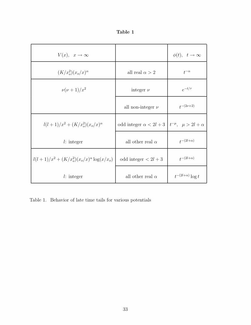
Table 1

V (x), x→ ∞ φ(t), t→ ∞

(K/x2o)(xo/x)

α all real α > 2 t−α

ν(ν + 1)/x2 integer ν e−t/τ

all non-integer ν t−(2ν+2)

l(l + 1)/x2 + (K/x2o)(xo/x)

α odd integer α < 2l + 3 t−µ, µ > 2l + α

l: integer all other real α t−(2l+α)

l(l + 1)/x2 + (K/x2o)(xo/x)

α log(x/xo) odd integer < 2l + 3 t−(2l+α)

l: integer all other real α t−(2l+α) log t

Table 1. Behavior of late time tails for various potentials

33

FIGURE CAPTIONS

Fig. 1 Generic time dependence of φ(x1, t) at a fixed spatial point x1, evolving from an

initial gaussian φ and initial φ = 0. The time evolution is governed by the Klein-

Gordon equation (1.1). The potential in this case is V (x) ∼ l(l + 1)/x2 + (log x)/x3

with l = 1. (a) Shorter time scale to show the prompt contributions; (b) longer time

scale to show the late time behavior.

Fig. 2 Singularity structure of G(x, y;ω) in the lower-half ω-plane, and the various contri-

butions to the Green’s function G(x, y; t).

Fig. 3 A spacetime diagram illustrating heuristically the different contributions GL, GQ

and GP (see text for definition) to the Green’s function.

Fig. 4 log |φ(x1, t)| versus log t for potentials with ν = 0 and a power-law V , which go as

xα−2o /xα as x → ∞. (a) (i) xo = 1, α = 3; (ii) xo = 100, α = 3 and (b) (i) xo = 1,

α = 2.5; (ii) xo = 1, α = 5.7. Solid lines are numerical results, which agree very well

with the analytical results (dashed lines).

Fig. 5 log |φ(x1, t)| versus log t for an inverse-square-law potential V (x) ∼ ν(ν + 1)/x2. (i)

ν = 1.01 and (ii) ν = 1. Solid lines are numerical results. For ν = 1.01, φ decreases as

t−µ with µ ≃ 4.03 which is in excellent agreement with the analytical result of t−(2+2ν)

(dashed line), derived in Section V. For ν = 1, φ decreases faster than any power

law, again agreeing with the theoretical prediction. For clarity, case (ii) is shifted

downwards by 8.0.

Fig. 6 A|φ(x1, t)|t2l+α versus log t for several potentials V (x) ∼ l(l + 1)/x2 + log x/xα. (i)

l = 0, α = 3; (ii) l = 1, α = 2.9; (iii) l = 1, α = 3; (iv) l = 1, α = 3.1. For clarity, the

data are multiplied by a constant A with (i) A = 10−9; (ii) and (iii) A = 5.6 × 10−10;

(iv) A = 5.86×10−10. The sloping straight lines observed at late times in cases (i), (ii)

and (iii) indicate the existence of a log t factor. Case (iv) is an exception, in which the

34

nearly zero asymptotic slope shows that the tail is a simple power law. The numerical

evolutions (solid lines) are indistinguishable from the analytical results (dashed lines)

for log t > 9.5.

Fig. 7 log |φ(x1, t)| versus log t for various potentials of the form 2/x2 + 1/xα as x → ∞.

(i) α = 2.9; (ii) α = 3.0; (iii) α = 3.1. To make the three sets of lines stagger, vertical

shifts have been applied. The generic late time behavior is t−µ and µ ≃ 2+α except in

case (ii) in which µ jumps discontinuously to 2α. Solid lines are numerical evolutions

while dashed lines are analytical results, derived in Section VI. In cases (i) and (iii),

the analytical results are completely specified both in form and magnitude; in case

(ii), only the form is known and the magnitude is fitted to the numerical result.

Fig. 8 Aφ(x, tL) versus x at a fixed time tL for the same potentials plotted in Fig. 4.

The numerical evolutions (solid lines) agree very well with the theoretical estimates

(pluses). (i) xo = 1, α = 3; (ii) xo = 100, α = 3; (iii) xo = 1, α = 2.5; (iv) xo = 1,

α = 5.7. The data are multiplied by a constant A for clarity. (i) A = 5 × 104; (ii)

A = 106; (iii) A = 103; (iv) A = 2 × 1015.

Fig. 9 Aφ(x, tL) versus x for various potentials of the form 2/x2 + (c1 log x + c2)/xα as

x → ∞. Solid lines are numerical results while the pluses are theoretical estimates.

(i) c1 = 1, c2 = 0, α = 3; (ii) c1 = 0, c2 = 1, α = 3.3; (iii) c1 = 0, c2 = 1, α = 4; (iv)

c1 = 0, c2 = 1, α = 5. The data are multiplied by a constant A for clarity. (i) A = 108;

(ii) A = 1010; (iii) A = 1012; (iv) A = 1015.

Fig. 10 Ghost behavior observed in the numerical evolution of φ(x1, t) using a second-

order spatial differencing scheme. The potential used in this case is V (x) ∼ 2/x2 as

x→ ∞ and the expected late time behavior is an exponential decay as shown in Fig. 5

(which uses a higher-order spatial differencing scheme) and Section V. In the present

numerical evolution, however, a straight line portion indicating a time dependence of

t−6 is observed. The magnitude of this “ghost” tail decreases by a factor of 4 when the

35

spatial interval ∆x is halved (see Appendix A), showing that this tail is a numerical

artifact.

Fig. 11 Contour C for evaluating the integral IA defined in (C6).

36