arX

iv:m

ath/

0403

297v

1 [m

ath.

NA

] 18

Mar

200

4

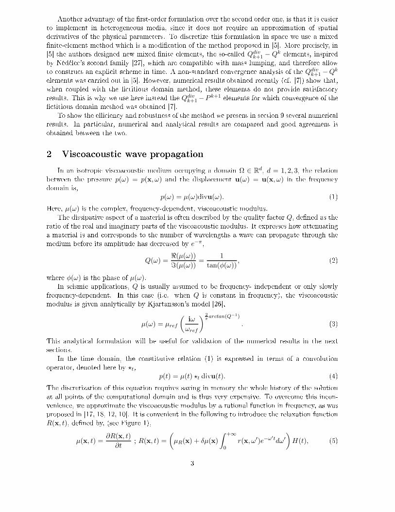
A time domain method for modeling vis oa ousti wavepropagationJean-Philippe Groby∗ Chrysoula Tsogka†February 1, 2008Abstra tIn many appli ations, and in parti ular in seismology, realisti propagation media dis-perse and attenuate waves. This dissipative behavior an be taken into a ount by usinga vis oa ousti propagation model, whi h in orporates a omplex and frequen y-dependentvis oa ousti modulus in the onstitutive relation. The main di ulty then lies in nding ane ient way to dis retize the onstitutive equation as it be omes a onvolution integral inthe time domain. To over ome this di ulty the usual approa h onsists in approximatingthe vis oa ousti modulus by a low-order rational fun tion of frequen y. We use here su h anapproximation and show how it an be in orporated in the velo ity-pressure formulation forvis oa ousti waves. This formulation is oupled with the titious domain method whi hpermit us to model e iently dira tion by obje ts of ompli ated geometry and with thePerfe tly Mat hed Layer Model whi h allows us to model wave propagation in unboundeddomains. The spa e dis retization of the problem is based on a mixed nite element methodand for the dis retization in time a 2nd order entered nite dieren e s heme is employed.Several numeri al examples illustrate the e ien y of the method.1 Introdu tionReal media attenuate and disperse propagating waves [19. Our aim in this paper is to developa numeri al method to model su h dissipative phenomena (dispersion plus attenuation) in thetime domain. To do so we onsider the linear vis oa ousti equation whi h is a onvolution in thetime domain, the vis oa ousti modulus being frequen y dependent. Therefore, in orporatingany arbitrary dissipation law in time-domain methods is in general omputationally intense. Theusual way to over ome this di ulty is to approximate the vis oa ousti modulus by a low-orderrational fun tion [17, 18, 12, 10. This leads to repla ing the onvolution integral by a set ofvariables, usually referred to as memory variables, whi h satisfy simple dierential equationsthat an be easily dis retized in the time domain.Several methods have been proposed in the literature for in orporating realisti attenuationlaws (e.g. frequen y-independent or weakly frequen y-dependent vis oa ousti modulus) intotime-domain methods [17, 18, 10, 12, 13, 14. We fo us our attention in this paper on the methodsproposed by Day and Minster (1984), Emmeri h and Korn (1987), and Blan h, Robertson andSymes (1995). All three methods use some approximation of the vis oa ousti modulus by a low-order rational fun tion. The rst approa h is based on the standard Padé approximation. The oe ients of the rational approximation are thus in prin iple known analyti ally. Numeri alresults obtained using this method show that the approximation is poor and the method provides∗Laboratoire de Mé anique de d'A oustique, Marseille, FRANCE, (grobylma. nrs-mrs.fr)†Mathemati s Department, Stanford University, USA, (tsogkamath.Stanford.EDU)1

satisfa tory results only for relatively short (in terms of the wavelength) propagation paths. These ond approa h is based on the rheologi al model of the generalized Maxwell body, whi h givesa physi al meaning to the oe ients of the rational approximation. They are interpreted asthe relaxation frequen ies and weight fa tors of the lassi al Maxwell bodies, whi h form thegeneralized Maxwell body. This method provides good numeri al results for long propagationpaths, but some parameters, namely the relaxation frequen ies are semi-empiri ally determined.Finally, the third method is based on the observation that for the frequen y-independent aseand for weakly attenuating materials the weight fa tors are only slowly varying and an beapproximated by a onstant. This method provides good numeri al results, but also involves asemi-empiri al hoi e of a parameter.Although, the previous methods give satisfa tory results in the ase of weakly-attenuatingmaterials they fail in media with large attenuation. This ase was onsidered in a re ent paper[1, where the authors propose an analyti method for omputing the best (optimal) rationalapproximation for the frequen y independent ase. They also propose a generalization of thealgorithm presented in [18 whi h leads to very good results in the ase of highly attenuatingmedia and a frequen y- dependent vis oa ousti modulus.After a brief overview of the basi theory des ribing wave propagation in vis oa ousti media(se tion 2), we des ribe in se tion 3 the approximations proposed in [17, [18 and [10.Considering long propagation paths, we test the performan e of the dierent approximationsand nd that the best method, using the smaller number of unknowns while providing satisfa -tory numeri al results and involving the least number of empiri ally determined values, is theone proposed by Emmeri h and Korn (1987). We thus hose this method for approximatingthe vis oa ousti modulus. Note that a slight variation of the method proposed in [18 is usedhere, based on a dierent way of distributing the relaxation frequen ies in the bandwidth of thein ident pulse.In se tion 4 we in orporate this approximation in the velo ity-pressure formulation for vis- oa ousti waves. Our hoi e of using the rst-order-in-time system of equations, instead of themore lassi al se ond-order one, is motivated by the use of the titious domain method andthe perfe tly mat hed absorbing layer te hnique. In [3 the authors proposed a similar approa husing the mixed velo ity-stress formulation for modeling wave propagation in vis oelasti media.The titious domain method (also alled the domain embedding method) has been devel-oped for solving problems involving omplex geometries [2, 22, 23, 21, 24, and, in parti ular,for wave propagation problems [15, 20, 29, 6. In the framework of seismi wave propagationwe apply this method to model the boundary ondition on the surfa e of the earth (se tion 7).Its main feature is extending the solution to a domain with simple shape, independent of the omplex geometry, and to impose the boundary onditions with the introdu tion of a Lagrangemultiplier. Thus, the solution is determined by two types of unknowns, the extended unknowns,dened in the enlarged simple shape domain and the auxiliary variable, supported on the bound-ary of omplex geometry. The main advantage is that the mesh for omputing the extendedfun tions an now be hosen independently of the geometry of the boundary.The Perfe tly Mat hed Layers (PML) te hnique was introdu ed by Bérenger [8, 9 forMaxwell's equations and is now the most widely-used method for the simulation of ele tro-magneti waves in unbounded domains ( f. [34, 31, 28). It has also been extended to the aseof anisotropi a ousti waves [4, isotropi [25 and anisotropi elasti waves [16, 4. This te h-nique onsists in designing an absorbing layer, alled a perfe tly mat hed layer (PML), that hasthe property of generating no ree tion at the interfa e between the free medium and the arti- ial absorbing medium. This property allows the use of a very high damping parameter insidethe layer, and onsequently of a small layer width, while a hieving a near-perfe t absorption ofthe waves. We apply here the PML model in the ase of vis oa ousti waves (se tion 8).2

Another advantage of the rst-order formulation over the se ond order one, is that it is easierto implement in heterogeneous media, sin e it does not require an approximation of spatialderivatives of the physi al parameters. To dis retize this formulation in spa e we use a mixednite-element method whi h is a modi ation of the method proposed in [5. More pre isely, in[5 the authors designed new mixed nite elements, the so- alled Qdivk+1 − Qk elements, inspiredby Nédéle 's se ond family [27, whi h are ompatible with mass lumping, and therefore allowto onstru t an expli it s heme in time. A non-standard onvergen e analysis of the Qdiv

k+1 −Qkelements was arried out in [5. However, numeri al results obtained re ently ( f. [7) show that,when oupled with the titious domain method, these elements do not provide satisfa toryresults. This is why we use here instead the Qdivk+1 −P k+1 elements for whi h onvergen e of the titious domain method was obtained [7.To show the e ien y and robustness of the method we present in se tion 9 several numeri alresults. In parti ular, numeri al and analyti al results are ompared and good agreement isobtained between the two.2 Vis oa ousti wave propagationIn an isotropi vis oa ousti medium o upying a domain Ω ∈ R

d, d = 1, 2, 3, the relationbetween the pressure p(ω) = p(x, ω) and the displa ement u(ω) = u(x, ω) in the frequen ydomain is,p(ω) = µ(ω)divu(ω). (1)Here, µ(ω) is the omplex, frequen y-dependent, vis oa ousti modulus.The dissipative aspe t of a material is often des ribed by the quality fa tor Q, dened as theratio of the real and imaginary parts of the vis oa ousti modulus. It expresses how attenuatinga material is and orresponds to the number of wavelengths a wave an propagate through themedium before its amplitude has de reased by e−π,

Q(ω) =ℜ(µ(ω))

ℑ(µ(ω))=

1

tan(φ(ω)), (2)where φ(ω) is the phase of µ(ω).In seismi appli ations, Q is usually assumed to be frequen y- independent or only slowlyfrequen y-dependent. In this ase (i.e. when Q is onstant in frequen y), the vis oa ousti modulus is given analyti ally by Kjartansson's model [26,

µ(ω) = µref

(iω

ωref

) 2π

arctan(Q−1)

. (3)This analyti al formulation will be useful for validation of the numeri al results in the nextse tions.In the time domain, the onstitutive relation (1) is expressed in terms of a onvolutionoperator, denoted here by ⋆t,p(t) = µ(t) ⋆t divu(t). (4)The dis retization of this equation requires saving in memory the whole history of the solutionat all points of the omputational domain and is thus very expensive. To over ome this in on-venien e, we approximate the vis oa ousti modulus by a rational fun tion in frequen y, as wasproposed in [17, 18, 12, 10. It is onvenient in the following to introdu e the relaxation fun tion

R(x, t), dened by, (see Figure 1),µ(x, t) =

∂R(x, t)

∂t; R(x, t) =

(µR(x) + δµ(x)

∫ +∞

0r(x, ω′)e−ω′tdω′

)H(t), (5)3

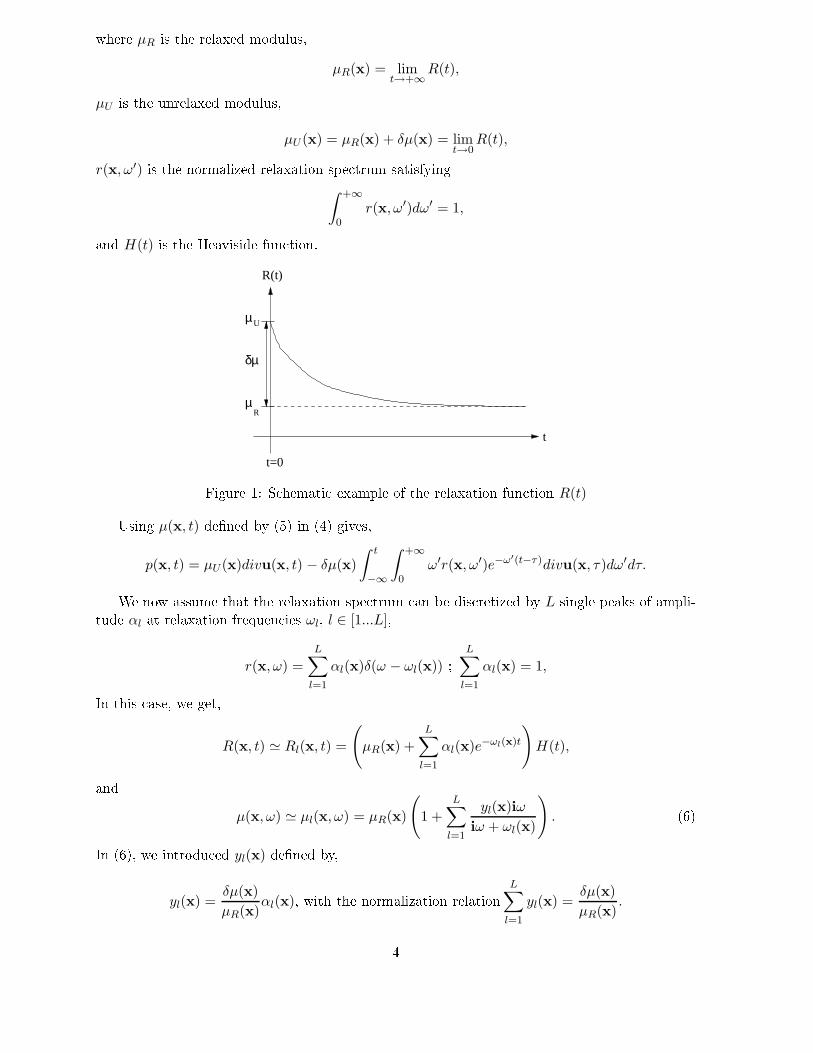
where µR is the relaxed modulus,µR(x) = lim

t→+∞R(t),

µU is the unrelaxed modulus,µU (x) = µR(x) + δµ(x) = lim

t→0R(t),

r(x, ω′) is the normalized relaxation spe trum satisfying∫ +∞

0r(x, ω′)dω′ = 1,and H(t) is the Heaviside fun tion.

R(t)

U

t=0

t

µ

µ

δµ

R

Figure 1: S hemati example of the relaxation fun tion R(t)Using µ(x, t) dened by (5) in (4) gives,p(x, t) = µU(x)divu(x, t) − δµ(x)

∫ t

−∞

∫ +∞

0ω′r(x, ω′)e−ω′(t−τ)divu(x, τ)dω′dτ.We now assume that the relaxation spe trum an be dis retized by L single peaks of ampli-tude αl at relaxation frequen ies ωl, l ∈ [1...L],

r(x, ω) =

L∑

l=1

αl(x)δ(ω − ωl(x)) ; L∑

l=1

αl(x) = 1,In this ase, we get,R(x, t) ≃ Rl(x, t) =

(µR(x) +

L∑

l=1

αl(x)e−ωl(x)t

)H(t),and

µ(x, ω) ≃ µl(x, ω) = µR(x)

(1 +

L∑

l=1

yl(x)iω

iω + ωl(x)

). (6)In (6), we introdu ed yl(x) dened by,

yl(x) =δµ(x)

µR(x)αl(x), with the normalization relation L∑

l=1

yl(x) =δµ(x)

µR(x).4

Noti e that equation (6) an be obtained if one assumes that µ(x, ω) an be approximated by arational fun tion of (iω),µ(x, ω) ≃ µl(x, ω) =

PL(x, iω)

QL(x, iω), (7)with PL and QL being polynomials of degree L in (iω). Then (6) an be interpreted as anexpansion of (7) into partial fra tions [18. Thus approximating the vis oa ousti modulus by arational fun tion is equivalent to approximating the relaxation spe trum by a dis rete one.For omputational reasons, it is natural to sear h for rational fun tion approximations of thevis oa ousti modulus, whi h minimize the ratio: number of unknowns/a ura y. We thereforeaddress in the following the question of nding an a urate low-order approximation of thevis oa ousti modulus.3 Approximation of the vis oa ousti modulusWe now briey introdu e the dierent approximation methods previously proposed in theliterature.3.1 Padé approximation methodThe use of the simple Padé approximation in the framework of vis oa ousti wave propaga-tion was proposed in [17. Letting z = −

1

iωand introdu ing,

χ(x, z) =

∫ +∞

0

ω′r(x, ω′)

1 − ω′zdω′,

µ(x, ω) an be re-written in the following form,µ(x, ω) = µU (x) + δµ(x)zχ(x, z).The Padé approximation is then used for expanding χ(x, z) into a rational fun tion with nu-merator of degree L− 1 and denominator of degree L. Using the well-known ([30, 11) relationsbetween Padé approximations and orthogonal polynomials one gets,

χ(x, z) =

L∑

l=1

λl(x)

1 − ωl(x)z,where ωl are the zeros of the orthogonal polynomial PL, and λl are the residuals given by,

λl(x) =kL

kL−1PL−1(ωl(x))P ′n(ωl(x))

,

kL being the leading oe ient of PL and where the prime denotes the derivative of PL. Re allthat the orthogonal polynomials are dened by,∫ Ω2

Ω1Pn(ω′)Pm(ω′)ω′r(ω′)dω′ = δmn,where δmn is the Krone ker symbol. When the quality fa tor is onstant over a frequen yband, λl and ωl an be obtained in losed form. Moreover, when Q ≪ 1, the relaxation spe trum5

r(x, ω) is proportional to ω−1. Assuming that r(x, ω) is zero outside the frequen y interval[Ω1,Ω2] we obtain the approximation,

µ(x, ω) ≃ µl(ω) = µU

(1 −

Ω2 − Ω1

πQ

L∑

l=1

νl(x)

iω + ωl(x)

), (8)where ωl =

1

2[xl(Ω2 − Ω1) + Ω2 + Ω1], xl and νl being respe tively the zeros and weights ofthe Legendre polynomials. Noti e that the relaxation frequen ies ωl are in this ase equidistanton a linear s ale. The main advantage of this approximation is that all data are analyti allydetermined. For more details on this method the reader an refer to [17.3.2 Generalized Maxwell Body approximation methodWe des ribe here the method proposed in [18. First let us re-write (6) as,

µl(x, ω) = µR(x) + δµ(x)

L∑

l=1

αl(x)iω

iω + ωl(x). (9)Ea h term of (9) an be interpreted as a lassi al Maxwell body with vis osity αl

δµ

ωland elasti modulus αlδµ. The term µR in (9) represents an additional elasti element. The Q-law for thegeneralized Maxwell body approximation an be obtained from (9),

Q(x, ω)−1 =ℑ(µ(x, ω))

ℜ(µ(x, ω))=

∑Ll=1 yl(x)

ωωl(x)

1+( ωωl(x)

)2

1 +∑L

l=1 yl(x)( ω

ωl(x))2

1+( ωωl(x)

)2

. (10)Assuming now that δµ ≪ µR, (10) be omes,Q(x, ω)−1 ⋍

δµ(x)

µR(x)

L∑

l=1

αl(x)

ωωl(x)

1 + ( ωωl(x))

2. (11)This means that Q(ω)−1 is approximately the sum of n Debye fun tions with maxima αl

δµ

2µRlo ated at frequen ies ωl. If Q is fairly onstant in a frequen y band, the most natural hoi e forthe relaxation frequen ies ωl is a logarithmi equidistant distribution. In this ase, to obtain agood approximation of Q(ω)−1, the distan e between two adja ent relaxation frequen ies shouldbe hosen smaller or equal to the half-width of the Debye fun tion (1.144 de ades). In [18two ways for hoosing ωl were proposed: ωl an be hosen logarithmi ally-equidistant in thefrequen y band [Ω1,Ω2] or determined by ωl =2ωdom

10lwhere ωdom is the dominant ( entral)frequen y of the sour e onsidered in the simulations. In both ases, the oe ients yl areobtained by solving the overdetermined linear system

L∑

l=1

yl(x)ωk(x)ωl(x) − Q−1(x, ωk(x))ωk(x)

ωl(x)2 + ωk(x)2= Q−1(x, ωk(x)), k ∈ [1, 2, ..K], (12)where, ωk are dened by

ω1 = Ω1,

ωk+1 = ωk(Ω2

Ω1)

12 .Let us remark that the determination of ωl for this approximation is based on an empiri alstudy. 6

3.3 The τ-methodThis method, proposed in [10 is based on the observation that dissipation due to only oneMaxwell Body an be determined by a unique dimensionless parameter τ . More pre isely, forQ ≫ 1 and L = 1, equation (11) be omes,

Q(x, ω)−1 =

ωω1(x)τ(x)

1 + ( ωω1(x))

2,where τ = y1 ≪ 1. It is then easy to see ( f. [10), that ω1 essentially determines thefrequen y behavior of Q while τ determines its magnitude. In the general ase for L > 1, andwhen one seeks an approximation of a onstant Q value, yl are quasi- onstantand equation (11) an be approximated by,

Q(x, ω)−1 =

L∑

l=1

ωωl(x)τ(x)

1 + ( ωωl(x))

2. (13)In (13), Q(ω)−1 is linear in τ . One an therefore nd the best approximation, in the least-squaressense, over a predened frequen y range to any Q0 by minimizing over τ the expression,

J =

∫ Ω2

Ω1

(Q−1(ω, ωl, τ) − Q−10 )2dω. (14)The approximation of the vis oa ousti modulus in this ase is,

µl(x, ω) = µR(x)

(1 +

L∑

l=1

τ(x)iω

iω + ωl(x)

). (15)The relaxation frequen ies ωl are hosen, as for the Generalized Maxwell Body method, equidis-tant on a logarithmi s ale. Equation (15) leads in general to an over-estimation of the valueof Q. Thus the authors in [10 suggest to use in the denition of J (14) a value for Q0 slightlysmaller than the desired one. This value is also hosen empiri ally.3.4 Comparison of the dierent approximation methodsTo test the a ura y of the dierent approximation methods previously presented, we om-pute the response of a one-dimensional vis oa ousti homogeneous medium to the followingpulse,

s(t) = sin

(2πt

T

)− 0.5sin

(4πt

T

) for 0 < t < T , T = 0.3s. (16)The solution is obtained by onvolving the sour e fun tion s(t) with the dissipation operatorD(t) (the Green's fun tion for the 1D problem). For an arbitrary dissipation law, the Fouriertransform D(ω) of D(t) is given by [18,

D(ω) = eiωt⋆Q(ωr)

(1− c(ωr)

ν(ω)

)

, (17)where c(ωr) is the phase velo ity at the referen e frequen y ωr, ν(ω) the omplex velo ity, andt⋆ =

x

c(ωr)Q(ωr)the dissipation time. For a frequen y independent Q, the value of c(ωr)

ν(ω)=

|µ(ωr)|

µ(ω), 7

0.5 1 1.5 2 2.5 3−0.2

0

0.2

0.4

0.6

0.8

1

1.2

Dissipation time

Padeτ −Cstmethod 1method2

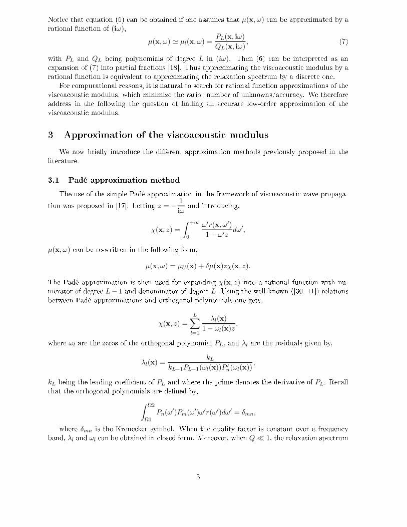
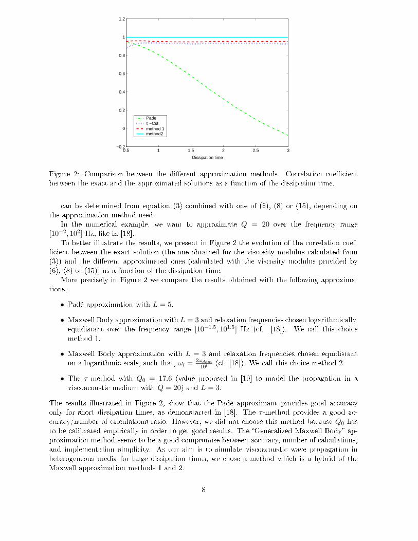
Figure 2: Comparison between the dierent approximation methods. Correlation oe ientbetween the exa t and the approximated solutions as a fun tion of the dissipation time. an be determined from equation (3) ombined with one of (6), (8) or (15), depending onthe approximation method used.In the numeri al example, we want to approximate Q = 20 over the frequen y range[10−2, 102] Hz, like in [18.To better illustrate the results, we present in Figure 2 the evolution of the orrelation oef- ient between the exa t solution (the one obtained for the vis osity modulus al ulated from(3)) and the dierent approximated ones ( al ulated with the vis osity modulus provided by(6), (8) or (15)) as a fun tion of the dissipation time.More pre isely in Figure 2 we ompare the results obtained with the following approxima-tions,

• Padé approximation with L = 5.• Maxwell Body approximation with L = 3 and relaxation frequen ies hosen logarithmi ally-equidistant over the frequen y range [10−1.5, 101.5] Hz ( f. [18). We all this hoi emethod 1.• Maxwell Body approximation with L = 3 and relaxation frequen ies hosen equidistanton a logarithmi s ale, su h that, ωl = 2ωdom

10l ( f. [18). We all this hoi e method 2.• The τ -method with Q0 = 17.6 (value proposed in [10 to model the propagation in avis oa ousti medium with Q = 20) and L = 3.The results illustrated in Figure 2, show that the Padé approximant provides good a ura yonly for short dissipation times, as demonstarted in [18. The τ -method provides a good a - ura y/number of al ulations ratio. However, we did not hoose this method be ause Q0 hasto be alibrated empiri ally in order to get good results. The Generalized Maxwell Body ap-proximation method seems to be a good ompromise between a ura y, number of al ulations,and implementation simpli ity. As our aim is to simulate vis oa ousti wave propagation inheterogeneous media for large dissipation times, we hose a method whi h is a hybrid of theMaxwell approximation methods 1 and 2. 8

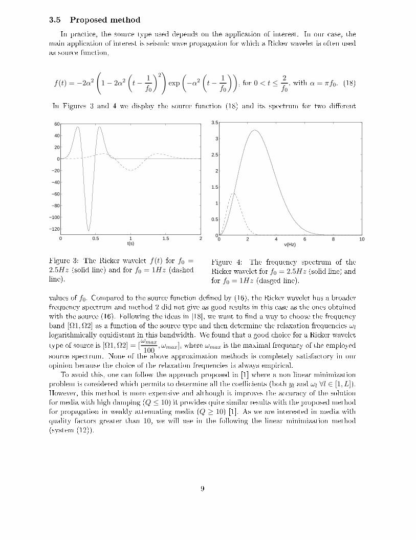
3.5 Proposed methodIn pra ti e, the sour e type used depends on the appli ation of interest. In our ase, themain appli ation of interest is seismi wave propagation for whi h a Ri ker wavelet is often usedas sour e fun tion,f(t) = −2α2

(1 − 2α2

(t −

1

f0

)2)

exp

(−α2

(t −

1

f0

)), for 0 < t ≤2

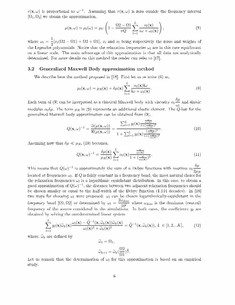
f0, with α = πf0. (18)In Figures 3 and 4 we display the sour e fun tion (18) and its spe trum for two dierent

0 0.5 1 1.5 2

−120

−100

−80

−60

−40

−20

0

20

40

60

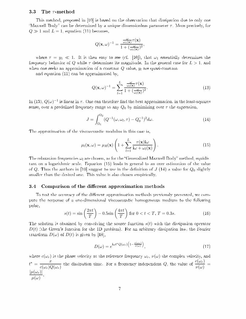
t(s)Figure 3: The Ri ker wavelet f(t) for f0 =2.5Hz (solid line) and for f0 = 1Hz (dashedline). 0 2 4 6 8 10

0

0.5

1

1.5

2

2.5

3

3.5

ν(Hz)Figure 4: The frequen y spe trum of theRi ker wavelet for f0 = 2.5Hz (solid line) andfor f0 = 1Hz (dasged line).values of f0. Compared to the sour e fun tion dened by (16), the Ri ker wavelet has a broaderfrequen y spe trum and method 2 did not give as good results in this ase as the ones obtainedwith the sour e (16). Following the ideas in [18, we want to nd a way to hoose the frequen yband [Ω1,Ω2] as a fun tion of the sour e type and then determine the relaxation frequen ies ωllogarithmi ally equidistant in this bandwidth. We found that a good hoi e for a Ri ker wavelettype of sour e is [Ω1,Ω2] = [ωmax

100, ωmax], where ωmax is the maximal frequen y of the employedsour e spe trum. None of the above approximation methods is ompletely satisfa tory in ouropinion be ause the hoi e of the relaxation frequen ies is always empiri al.To avoid this, one an follow the approa h proposed in [1 where a non-linear minimizationproblem is onsidered whi h permits to determine all the oe ients (both yl and ωl ∀l ∈ [1, L]).However, this method is more expensive and although it improves the a ura y of the solutionfor media with high damping (Q ≤ 10) it provides quite similar results with the proposed methodfor propagation in weakly attenuating media (Q ≥ 10) [1. As we are interested in media withquality fa tors greater than 10, we will use in the following the linear minimization method(system (12)).

9

4 The mixed velo ity-pressure formulationBy in orporating (6) into (1) we get,p(x, ω) = µR(x)div(u(x, ω)) + µR(x)

L∑

l=1

yl(x)iω

iω + ωl(x)div(u(x, ω)). (19)We now introdu e the memory variables ηl dened by,

(iω + ωl(x))ηl(x, ω) = µR(x)yl(x)div(v(x, ω)), (20)where v is the velo ity, i.e., the time derivative of the displa ement u. Equation (20) in the timedomain be omes,∂ηl(x, t)

∂t+ ωl(x)ηl(x, t) = µR(x)yl(x)div(v(x, t)). (21)Using the denition of ηl and multiplying (19) by (iω), we get,

(iω)p(x, ω) = µR(x)div(v(x, ω)) +L∑

l=1

(iω)ηl(x, ω),or equivalently in the time domain,∂p

∂t= µRdiv(v) +

n∑

l=1

∂ηl

∂t. (22)Combining (22), (21) and the equation of motion, we obtain our nal system of equations,

ρ∂v

∂t−∇p = f in Ω×]0, T ],

∂p

∂t−

n∑

l=1

∂ηl

∂t= µRdiv(v) in Ω×]0, T ],

∂ηl

∂t+ ωlηl = µRyldiv(v),∀l in Ω×]0, T ].

(23)Equivalently, one an hose to eliminate the pressure and obtain a se ond-order-in-time equationfor the displa ement by introdu ing adequate memory variables [18. We prefer, however, therst-order velo ity-pressure formulation for the following reasons,• It an be oupled with the titious domain method for taking into a ount dira tion byobje ts of ompli ated geometry.• A perfe tly mat hed layer model (PML) an be written for this system. This permits usto simulate e iently wave propagation in unbounded domains.• This system is easier to implement in heterogeneous media, sin e it does not require anapproximation of the spatial derivatives of the physi al parameters.An equivalent rst-order velo ity-pressure system is proposed in [12 and [10. In [12 the authorsused a pseudospe tral method for the dis retization while in [10 a staggered nite dieren es heme was used. Our aim being to ouple this system with the titious domain method,we propose here instead the use of a mixed-nite element method on regular grids. A similarapproa h was proposed in [3 where the authors use a mixed-nite element method to dis retizethe velo ity-stress formulation for vis oelasti wave propagation.10

5 Dis retisationA mixed formulation asso iated to equations (23) is given by,

Find (v, p,H) :]0, T [7−→ X × M × (M)L s.t. :d

dt(ρv,w) + b(w, p) = (f ,w), ∀w ∈ X,

d

dt(

1

µRp, q) −

L∑

l=1

d

dt(

1

µRηl, q) − b(v, q) = 0, ∀q ∈ M,

d

dt(

1

µRylηl, q) + (

ωl

µRylηl, q) − b(v, q) = 0, ∀l, ∀q ∈ M,

(24)where H is the L-dimensional ve tor with omponents ηl, and

b(w, q) =

∫

Ωq divw dx, ∀(w, q) ∈ X × M.The fun tional spa es are X = H(div; Ω), and M = L2(Ω).We now introdu e some nite element spa es Xh ⊂ X, and Mh ⊂ M of dimensions N1 and N2respe tively. The semi-dis retization in the spa e of problem (24) is,

(Vh, Ph,Hh) ∈ L2(0, T ; IRN1) × L2(0, T ; IRN2) × L2(0, T ; (IRN2)L) s.t. :Mv

dVh

dt+ BhPh = Fh,

MpdPh

dt−

L∑

l=1

Mpd(Hh)l

dt− BT

h Vh = 0,

Myd(Hh)l

dt+ Mω(Hh)l − BT

h Vh = 0, ∀l,

(25)where BT

h denotes the transpose of Bh.In pra ti e, we only onsider regular domains in IRd, d = 1, 2 that an be dis retized with auniform mesh Th omposed by segments or squares of size h, depending on the dimension of theproblem. The nite element spa es we use areXh =

wh in X / ∀K ∈ Th,wh |K ∈ (Q1)

d

,andMh =

qh ∈ L2 / ∀K ∈ Th, qh|K ∈ P0(K)

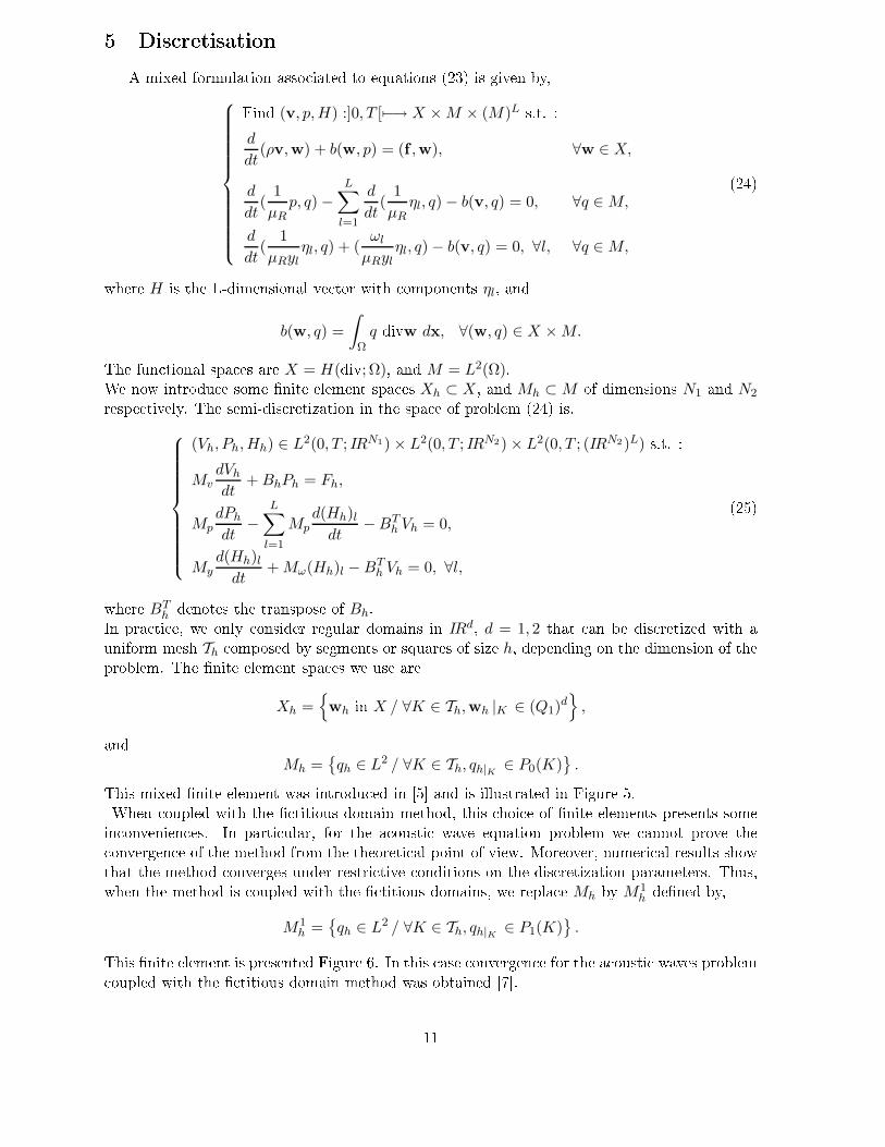
.This mixed nite element was introdu ed in [5 and is illustrated in Figure 5.When oupled with the titious domain method, this hoi e of nite elements presents somein onvenien es. In parti ular, for the a ousti wave equation problem we annot prove the onvergen e of the method from the theoreti al point of view. Moreover, numeri al results showthat the method onverges under restri tive onditions on the dis retization parameters. Thus,when the method is oupled with the titious domains, we repla e Mh by M1

h dened by,M1

h =qh ∈ L2 / ∀K ∈ Th, qh|K ∈ P1(K)

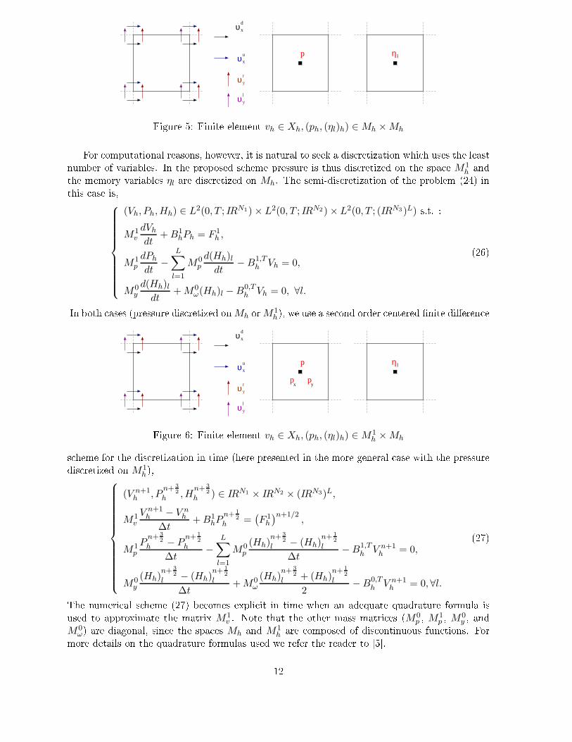
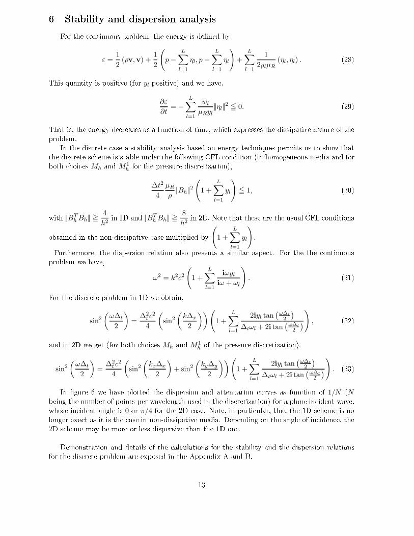
.This nite element is presented Figure 6. In this ase onvergen e for the a ousti waves problem oupled with the titious domain method was obtained [7.11

υx

d

υx

y

r

υy

l

u

υ

p η l

Figure 5: Finite element vh ∈ Xh, (ph, (ηl)h) ∈ Mh × MhFor omputational reasons, however, it is natural to seek a dis retization whi h uses the leastnumber of variables. In the proposed s heme pressure is thus dis retized on the spa e M1h andthe memory variables ηl are dis retized on Mh. The semi-dis retization of the problem (24) inthis ase is,

(Vh, Ph,Hh) ∈ L2(0, T ; IRN1) × L2(0, T ; IRN2) × L2(0, T ; (IRN3)L) s.t. :M1

v

dVh

dt+ B1

hPh = F 1h ,

M1p

dPh

dt−

L∑

l=1

M0p

d(Hh)ldt

− B1,Th Vh = 0,

M0y

d(Hh)ldt

+ M0ω(Hh)l − B0,T

h Vh = 0, ∀l.

(26)In both ases (pressure dis retized on Mh or M1

h), we use a se ond order entered nite dieren eυx

d

υx

y

r

υy

l

u

υ

p η

p p

l

x yFigure 6: Finite element vh ∈ Xh, (ph, (ηl)h) ∈ M1h × Mhs heme for the dis retization in time (here presented in the more general ase with the pressuredis retized on M1

h),

(V n+1h , P

n+ 32

h ,Hn+ 3

2h ) ∈ IRN1 × IRN2 × (IRN3)L,

M1v

V n+1h − V n

h

∆t+ B1

hPn+ 1

2h =

(F 1

h

)n+1/2,

M1p

Pn+ 3

2h − P

n+ 12

h

∆t−

L∑

l=1

M0p

(Hh)n+ 3

2l − (Hh)

n+ 12

l

∆t− B1,T

h V n+1h = 0,

M0y

(Hh)n+ 3

2l − (Hh)

n+ 12

l

∆t+ M0

ω

(Hh)n+ 3

2l + (Hh)

n+ 12

l

2− B0,T

h V n+1h = 0,∀l.

(27)The numeri al s heme (27) be omes expli it in time when an adequate quadrature formula isused to approximate the matrix M1

v . Note that the other mass matri es (M0p , M1

p , M0y , and

M0ω) are diagonal, sin e the spa es Mh and M1

h are omposed of dis ontinuous fun tions. Formore details on the quadrature formulas used we refer the reader to [5.12

6 Stability and dispersion analysisFor the ontinuous problem, the energy is dened byε =

1

2(ρv,v) +

1

2

(p −

L∑

l=1

ηl, p −

L∑

l=1

ηl

)+

L∑

l=1

1

2ylµR(ηl, ηl) . (28)This quantity is positive (for yl positive) and we have,

∂ε

∂t= −

L∑

l=1

wl

µRyl||ηl||

2 ≦ 0. (29)That is, the energy de reases as a fun tion of time, whi h expresses the dissipative nature of theproblem.In the dis rete ase a stability analysis based on energy te hniques permits us to show thatthe dis rete s heme is stable under the following CFL ondition (in homogeneous media and forboth hoi es Mh and M1h for the pressure dis retization),

∆t2

4

µR

ρ||Bh||

2

(1 +

L∑

l=1

yl

)≦ 1, (30)with ||BT

h Bh|| ≧4

h2in 1D and ||BT

h Bh|| ≧8

h2in 2D. Note that these are the usual CFL onditionsobtained in the non-dissipative ase multiplied by (1 +

L∑

l=1

yl

).Furthermore, the dispersion relation also presents a similar aspe t. For the the ontinuousproblem we have,ω2 = k2c2

(1 +

L∑

l=1

iωyl

iω + ωl

). (31)For the dis rete problem in 1D we obtain,

sin2

(ω∆t

2

)=

∆2t c

2

4

(sin2

(k∆x

2

))(1 +

L∑

l=1

2iyl tan(

ω∆t

2

)

∆tωl + 2i tan(

ω∆t

2

))

, (32)and in 2D we get (for both hoi es Mh and M1h of the pressure dis retization),

sin2

(ω∆t

2

)=

∆2t c

2

4

(sin2

(kx∆x

2

)+ sin2

(ky∆y

2

))(1 +

L∑

l=1

2iyl tan(

ω∆t

2

)

∆tωl + 2i tan(

ω∆t

2

))

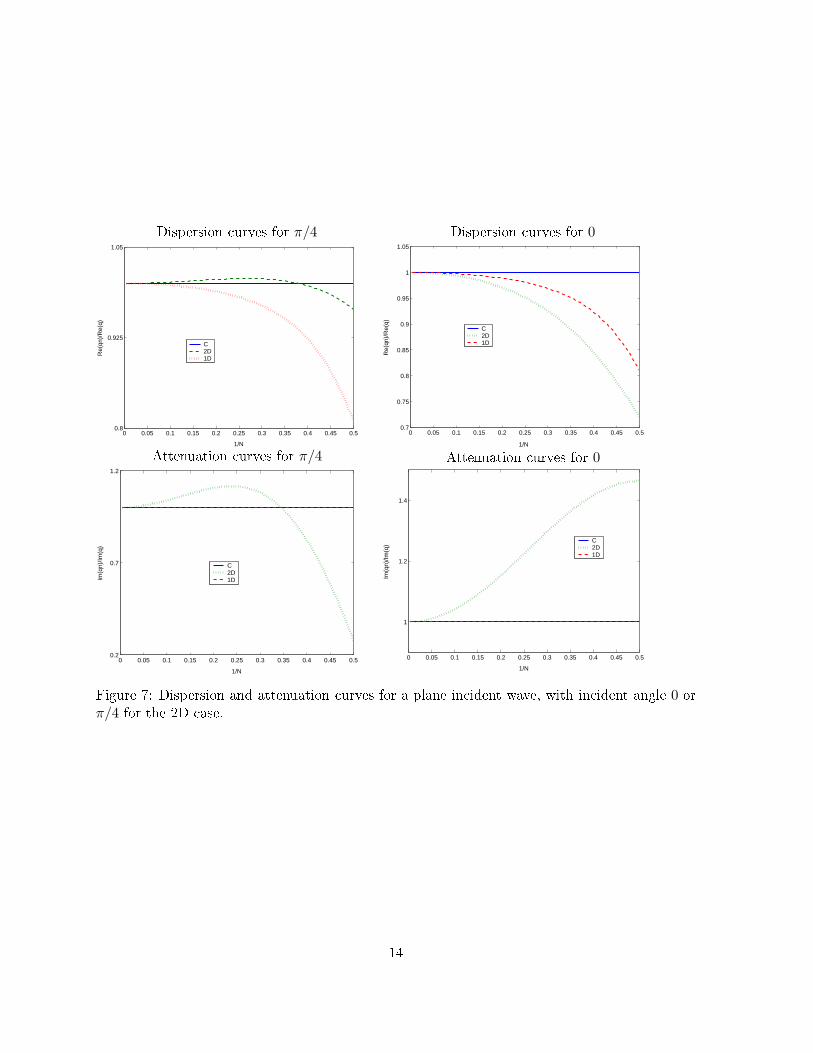
. (33)In gure 6 we have plotted the dispersion and attenuation urves as fun tion of 1/N (Nbeing the number of points per wavelength used in the dis retization) for a plane in ident wave,whose in ident angle is 0 or π/4 for the 2D ase. Note, in parti ular, that the 1D s heme is nolonger exa t as it is the ase in non-dissipative media. Depending on the angle of in iden e, the2D s heme may be more or less dispersive than the 1D one.Demonstration and details of the al ulations for the stability and the dispersion relationsfor the dis rete problem are exposed in the Appendix A and B.13

Dispersion urves for π/4 Dispersion urves for 0

0 0.05 0.1 0.15 0.2 0.25 0.3 0.35 0.4 0.45 0.50.8

0.925

1.05

1/N

Re(

qn)/

Re(

q)

C2D1D

0 0.05 0.1 0.15 0.2 0.25 0.3 0.35 0.4 0.45 0.50.7

0.75

0.8

0.85

0.9

0.95

1

1.05

1/N

Re(

qn)/

Re(

q)

C2D1D

Attenuation urves for π/4 Attenuation urves for 0

0 0.05 0.1 0.15 0.2 0.25 0.3 0.35 0.4 0.45 0.50.2

0.7

1.2

1/N

Im(q

n)/Im

(q)

C2D1D

0 0.05 0.1 0.15 0.2 0.25 0.3 0.35 0.4 0.45 0.5

1

1.2

1.4

1/N

Im(q

n)/Im

(q)

C2D1D

Figure 7: Dispersion and attenuation urves for a plane in ident wave, with in ident angle 0 orπ/4 for the 2D ase.

14

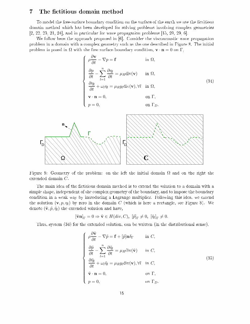
7 The titious domain methodTo model the free-surfa e boundary ondition on the surfa e of the earth we use the titiousdomain method whi h has been developed for solving problems involving omplex geometries[2, 22, 23, 21, 24, and in parti ular for wave propagation problems [15, 20, 29, 6.We follow here the approa h proposed in [6. Consider the vis oa ousti wave propagationproblem in a domain with a omplex geometry su h as the one des ribed in Figure 8. The initialproblem is posed in Ω with the free-surfa e boundary ondition, v · n = 0 on Γ,

ρ∂v

∂t−∇p = f in Ω,

∂p

∂t−

n∑

l=1

∂ηl

∂t= µRdiv(v) in Ω,

∂ηl

∂t+ ωlηl = µRyldiv(v),∀l in Ω,

v · n = 0, on Γ,

p = 0, on ΓD.

(34)

DΓ

n

Γ

Ω

DΓ

CFigure 8: Geometry of the problem: on the left the initial domain Ω and on the right theextended domain C.The main idea of the titious domain method is to extend the solution to a domain with asimple shape, independent of the omplex geometry of the boundary, and to impose the boundary ondition in a weak way by introdu ing a Lagrange multiplier. Following this idea, we extendthe solution (v, p, ηl) by zero in the domain C (whi h is here a re tangle, see Figure 8). Wedenote (v, p, ηl) the extended solution and have,[vn]Γ = 0 ⇒ v ∈ H(div,C), [p]Γ 6= 0, [ηl]Γ 6= 0.Thus, system (34) for the extended solution, an be written (in the distributional sense),

ρ∂v

∂t−∇p = f + [p]nδΓ in C,

∂p

∂t−

n∑

l=1

∂ηl

∂t= µRdiv(v) in C,

∂ηl

∂t+ ωlηl = µRyldiv(v),∀l in C,

v · n = 0, on Γ,

p = 0, on ΓD.

(35)15

In (35) we have two types of unknowns, the extended unknowns, dened in the simple shapedomain C and the auxiliary variable [p], dened on the boundary Γ. We introdu e λ = [p]as a new unknown dened on Γ. This unknown an be interpreted as a Lagrange multiplierasso iated with the boundary ondition on Γ. The variational formulation of the problem anthen be written as follows,

Find (v, p,H, λ) :]0, T [7−→ H(div;C) × L2(C) × (L2(C))L × H1/2(Γ) s.t.d

dt(ρv,w) + b(w, p) − bΓ(λ,w) = (f ,w), ∀w ∈ H(div;C),

d

dt(

1

µRp, q) −

L∑

l=1

d

dt(

1

µRηl, q) − b(v, q) = 0, ∀q ∈ L2(C),

d

dt(

1

µRylηl, q) + (

ωl

µRylηl, q) − b(v, q) = 0, ∀l, ∀q ∈ L2(C),

bΓ(µ,v) = 0, ∀µ ∈ H1/2(Γ),wherebΓ(µ,w) =

∫

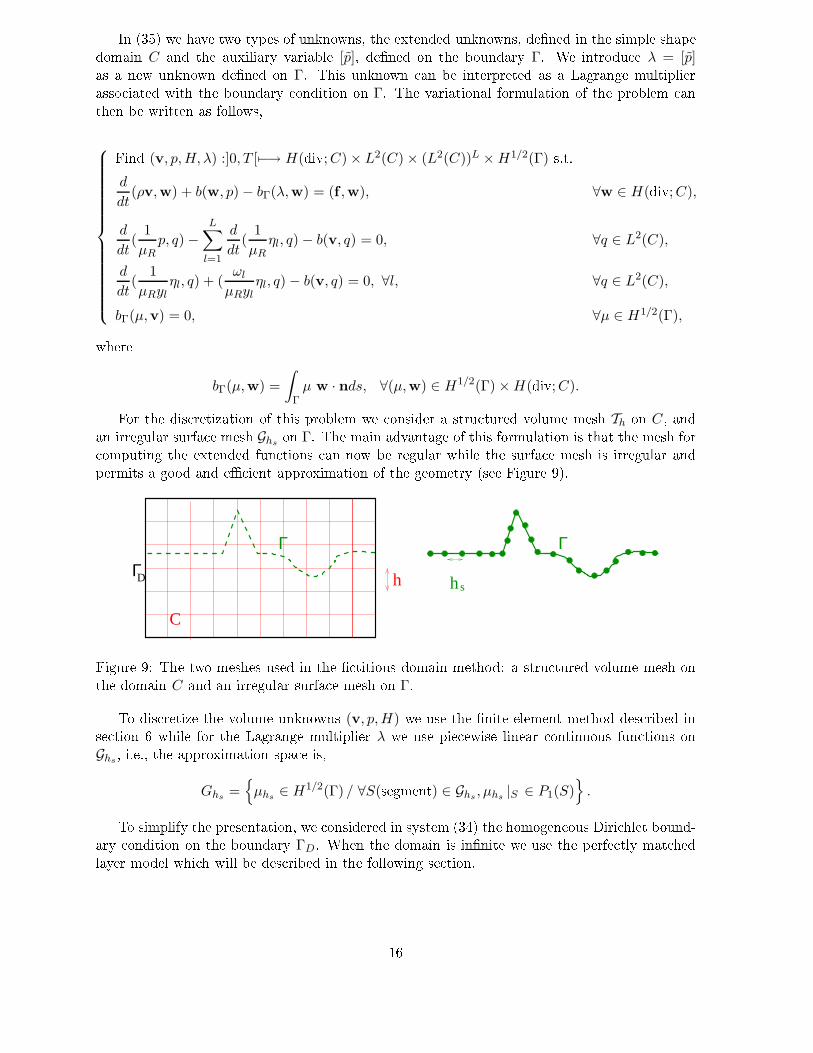
Γµ w · nds, ∀(µ,w) ∈ H1/2(Γ) × H(div;C).For the dis retization of this problem we onsider a stru tured volume mesh Th on C, andan irregular surfa e mesh Ghs

on Γ. The main advantage of this formulation is that the mesh for omputing the extended fun tions an now be regular while the surfa e mesh is irregular andpermits a good and e ient approximation of the geometry (see Figure 9).h hs

DΓ

C

Γ Γ

Figure 9: The two meshes used in the titious domain method: a stru tured volume mesh onthe domain C and an irregular surfa e mesh on Γ.To dis retize the volume unknowns (v, p,H) we use the nite element method des ribed inse tion 6 while for the Lagrange multiplier λ we use pie ewise linear ontinuous fun tions onGhs

, i.e., the approximation spa e is,Ghs

=µhs

∈ H1/2(Γ) / ∀S(segment) ∈ Ghs, µhs

|S ∈ P1(S)

.To simplify the presentation, we onsidered in system (34) the homogeneous Diri hlet bound-ary ondition on the boundary ΓD. When the domain is innite we use the perfe tly mat hedlayer model whi h will be des ribed in the following se tion.16

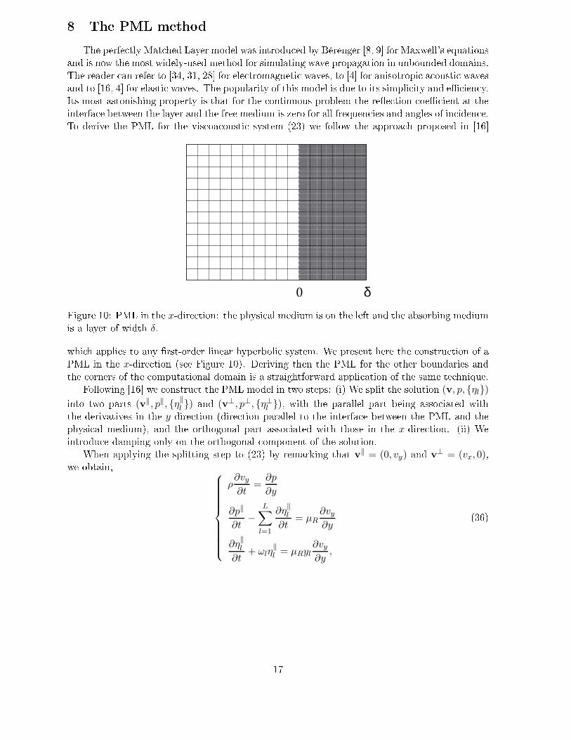
8 The PML methodThe perfe tly Mat hed Layer model was introdu ed by Bérenger [8, 9 for Maxwell's equationsand is now the most widely-used method for simulating wave propagation in unbounded domains.The reader an refer to [34, 31, 28 for ele tromagneti waves, to [4 for anisotropi a ousti wavesand to [16, 4 for elasti waves. The popularity of this model is due to its simpli ity and e ien y.Its most astonishing property is that for the ontinuous problem the ree tion oe ient at theinterfa e between the layer and the free medium is zero for all frequen ies and angles of in iden e.To derive the PML for the vis oa ousti system (23) we follow the approa h proposed in [16

δ0Figure 10: PML in the x-dire tion: the physi al medium is on the left and the absorbing mediumis a layer of width δ.whi h applies to any rst-order linear hyperboli system. We present here the onstru tion of aPML in the x-dire tion (see Figure 10). Deriving then the PML for the other boundaries andthe orners of the omputational domain is a straightforward appli ation of the same te hnique.Following [16 we onstru t the PML model in two steps: (i) We split the solution (v, p, ηl)into two parts (v‖, p‖, η‖l ) and (v⊥, p⊥, η⊥l ), with the parallel part being asso iated withthe derivatives in the y-dire tion (dire tion parallel to the interfa e between the PML and thephysi al medium), and the orthogonal part asso iated with those in the x-dire tion. (ii) Weintrodu e damping only on the orthogonal omponent of the solution.When applying the splitting step to (23) by remarking that v

‖ = (0, vy) and v⊥ = (vx, 0),we obtain,

ρ∂vy

∂t=

∂p

∂y

∂p‖

∂t−

L∑

l=1

∂η‖l

∂t= µR

∂vy

∂y

∂η‖l

∂t+ ωlη

‖l = µRyl

∂vy

∂y,

(36)

17

and

ρ∂vx

∂t=

∂p

∂x

∂p⊥

∂t−

L∑

l=1

∂η⊥l∂t

= µR∂vx

∂x

∂η⊥l∂t

+ ωlη⊥l = µRyl

∂vx

∂x,

(37)with p = p‖ + p⊥

ηl = η‖l + η⊥l , ∀l.

(38)To apply the damping on the orthogonal omponents it is simpler to onsider system (37) in thefrequen y domain. Then the PML onsists in repla ing the x-derivatives ∂x by iω

iω + d(x)∂x ( f.[16). Following this approa h, system (37) in the frequen y domain be omes,

(i) ρ(iω + d(x))∂vx =∂p

∂x

(ii) (iω + d(x))p⊥ −

L∑

l=1

(iω + d(x))η⊥l = µR∂vx

∂x

(iii) (iω)(iω + d(x))η⊥l + (iω + d(x))ωlη⊥l = (iω)µRyl

∂vx

∂x,

(39)where d(x) is the damping parameter whi h is equal to zero in the physi al medium and non-negative in the absorbing medium.We now introdu e new variables ηl dened by,iωηl = (iω + d(x))η⊥l , ∀l, (40)or equivalently in time domain,∂ηl

∂t=

∂η⊥l∂t

+ d(x)η⊥l , ∀l.Using (40) in (39) and going in the time domain we get,

ρ∂vx

∂t+ ρd(x)vx =

∂p

∂x

∂p⊥

∂t+ d(x)p⊥ −

L∑

l=1

∂ηl

∂t= µR

∂vx

∂x

∂ηl

∂t+ ωlηl = µRyl

∂vx

∂x.

(41)The nal system of equations for the PML is (41) together with (36), with p being dened byp = p‖ + p⊥. Note that the memory variables ηl do not appear, and only the omponent η

‖l andthe variables ηl do appear, in this system.Using a plane wave analysis, it an be shown ( f. [16) that this model generates no ree tionat the interfa e between the physi al and the absorbing medium and that the wave de reasesexponentially inside the layer. This property allows the use of a very high damping parameterinside the layer, and onsequently of a small layer width, while a hieving a near-perfe t absorp-tion of the waves. Note that for a nite-length absorbing layer there is some ree tion due tothe outer boundary of the PML. 18

Remark 1 To dis retize the PML we use the same s heme as for the interior domain.Remark 2 The damping d(x) is zero in the physi al domain and non negative in the absorbingmedium. In the numeri al simulations it is dened as in [16,d(x) =

0 for x < 0

log(

1R

) (n+1)√

µRρ

2δ (xδ )n for x ≥ 0

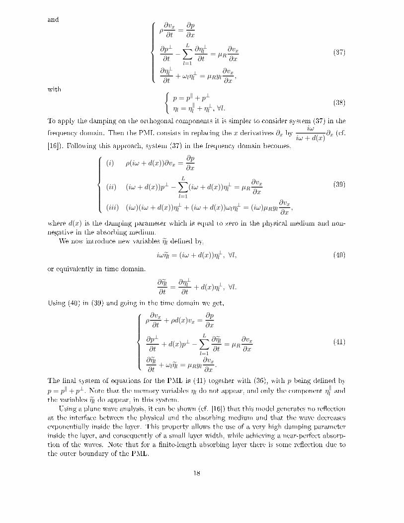
(42)where R is the theoreti al ree tion oe ient, δ the width of the PML and n = 4.In pra ti e, we take R = 5.0 10−7, and δ ≈ 30∆x (depending on the wavelength).9 Numeri al results9.1 S attering from a ir ular ylinderIn order to validate the proposed numeri al method we onsider in this se tion the anon-i al problem of a plane wave (Ri ker wavelet) striking a vis oa ousti homogeneous ir ular ylinder. The geometry of the problem is displayed in Figure 11. A homogeneous vis oa ous-ti ir ular ylinder of radius a (domain Ω2) is surrounded by a homogeneous non-dissipativemedium (domain Ω1). We denote by Γ1 the interfa e between the two domains Ω1 and Ω2. Thephysi al hara teristi s of the media are ρ1 = 1000Kgr/m3, c1 = 3050m/s, Q1 = +∞ in Ω1and ρ2 = 1800Kgr/m3, c2 = 3050m/s and Q2 = 30 in Ω2. The sour e fun tion used in thisexample is given by (18) with f0 = 2.5Hz. For this problem, the solution an be omputed byan analyti al method des ribed in what follows.ρ =1000Kg.m

ρ =1800Kg.m−3

−3

c =3050 m.s

c =3050 m.s

−1

−11

1

2

Ω

2

2

Ω1

1200 m

3500 m

3500 m

R2

R1

R3

Figure 11: The geometry of the problem: a homogeneous vis oa ousti ylinder of radius a(domain Ω2) embedded in a non-dissipative homogeneous medium (domain Ω1).Consider the following in ident plane wave (with in ident angle 0 ≤ θi < 2π),pi1(x) = Ai

0

n=∞∑

n=−∞

e−in(θi+ π2)Jn(k0r)exp(inθ); ∀x = (r cos(θ), r sin(θ)) ∈ Ω1. (43)19

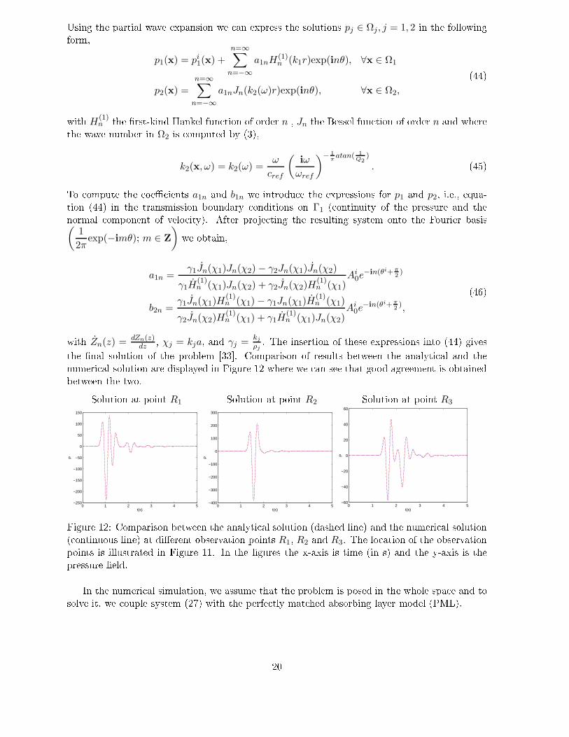
Using the partial wave expansion we an express the solutions pj ∈ Ωj, j = 1, 2 in the followingform,p1(x) = pi

1(x) +

n=∞∑

n=−∞

a1nH(1)n (k1r)exp(inθ), ∀x ∈ Ω1

p2(x) =n=∞∑

n=−∞

a1nJn(k2(ω)r)exp(inθ), ∀x ∈ Ω2,

(44)with H(1)n the rst-kind Hankel fun tion of order n , Jn the Bessel fun tion of order n and wherethe wave number in Ω2 is omputed by (3),

k2(x, ω) = k2(ω) =ω

cref

(iω

ωref

)− 1π

atan( 1Q2

)

. (45)To ompute the oe ients a1n and b1n we introdu e the expressions for p1 and p2, i.e., equa-tion (44) in the transmission boundary onditions on Γ1 ( ontinuity of the pressure and thenormal omponent of velo ity). After proje ting the resulting system onto the Fourier basis(1

2πexp(−imθ); m ∈ Z

) we obtain,a1n =

γ1Jn(χ1)Jn(χ2) − γ2Jn(χ1)Jn(χ2)

γ1H(1)n (χ1)Jn(χ2) + γ2Jn(χ2)H

(1)n (χ1)

Ai0e

−in(θi+ π2)

b2n =γ1Jn(χ1)H

(1)n (χ1) − γ1Jn(χ1)H

(1)n (χ1)

γ2Jn(χ2)H(1)n (χ1) + γ1H

(1)n (χ1)Jn(χ2)

Ai0e

−in(θi+ π2),

(46)with Zn(z) = dZn(z)dz , χj = kja, and γj =

kj

ρj. The insertion of these expressions into (44) givesthe nal solution of the problem [33. Comparison of results between the analyti al and thenumeri al solution are displayed in Figure 12 where we an see that good agreement is obtainedbetween the two.Solution at point R1 Solution at point R2 Solution at point R3

0 1 2 3 4 5−250

−200

−150

−100

−50

0

50

100

150

t(s)

P

0 1 2 3 4 5−400

−300

−200

−100

0

100

200

300

t(s)

P

0 1 2 3 4 5−60

−40

−20

0

20

40

60

t(s)

P

Figure 12: Comparison between the analyti al solution (dashed line) and the numeri al solution( ontinuous line) at dierent observation points R1, R2 and R3. The lo ation of the observationpoints is illustrated in Figure 11. In the gures the x-axis is time (in s) and the y-axis is thepressure eld.In the numeri al simulation, we assume that the problem is posed in the whole spa e and tosolve it, we ouple system (27) with the perfe tly mat hed absorbing layer model (PML).20

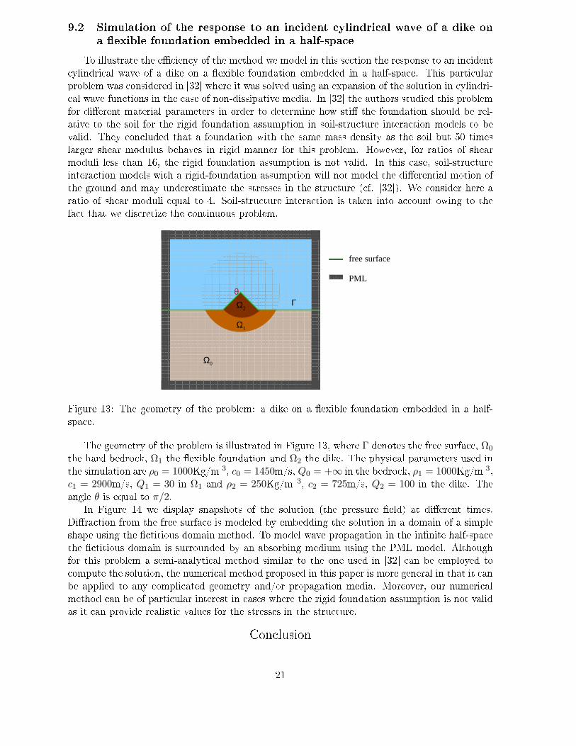
9.2 Simulation of the response to an in ident ylindri al wave of a dike ona exible foundation embedded in a half-spa eTo illustrate the e ien y of the method we model in this se tion the response to an in ident ylindri al wave of a dike on a exible foundation embedded in a half-spa e. This parti ularproblem was onsidered in [32 where it was solved using an expansion of the solution in ylindri- al wave fun tions in the ase of non-dissipative media. In [32 the authors studied this problemfor dierent material parameters in order to determine how sti the foundation should be rel-ative to the soil for the rigid foundation assumption in soil-stru ture intera tion models to bevalid. They on luded that a foundation with the same mass density as the soil but 50 timeslarger shear modulus behaves in rigid manner for this problem. However, for ratios of shearmoduli less than 16, the rigid foundation assumption is not valid. In this ase, soil-stru tureintera tion models with a rigid-foundation assumption will not model the dierential motion ofthe ground and may underestimate the stresses in the stru ture ( f. [32). We onsider here aratio of shear moduli equal to 4. Soil-stru ture intera tion is taken into a ount owing to thefa t that we dis retize the ontinuous problem.

0

Ω

Ω1

Ω2

PML

Γθ

free surface

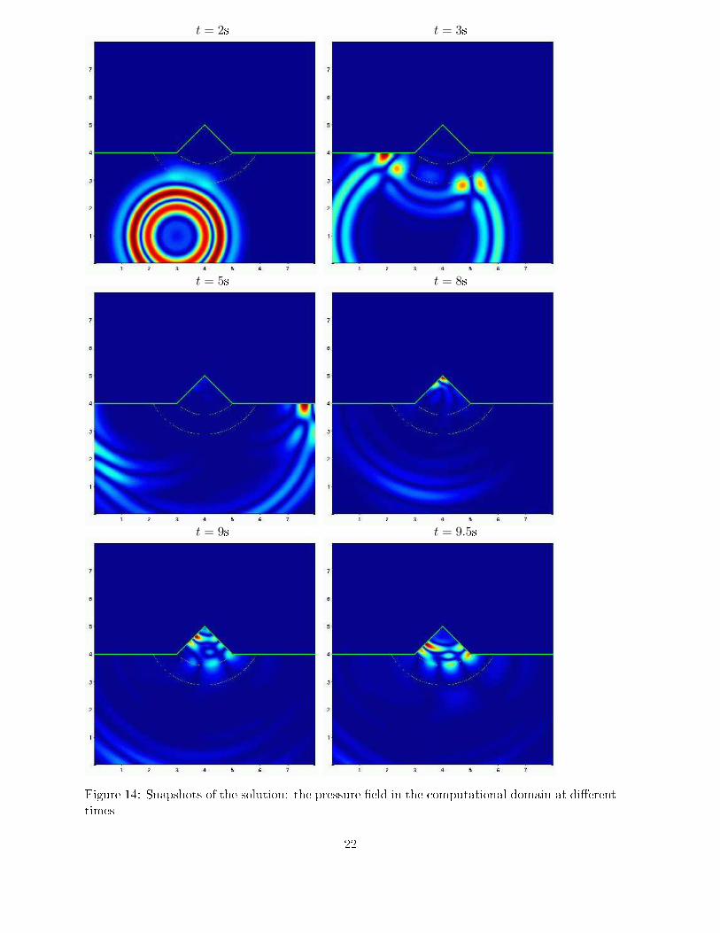
Figure 13: The geometry of the problem: a dike on a exible foundation embedded in a half-spa e.The geometry of the problem is illustrated in Figure 13, where Γ denotes the free surfa e, Ω0the hard bedro k, Ω1 the exible foundation and Ω2 the dike. The physi al parameters used inthe simulation are ρ0 = 1000Kg/m 3, c0 = 1450m/s, Q0 = +∞ in the bedro k, ρ1 = 1000Kg/m 3,c1 = 2900m/s, Q1 = 30 in Ω1 and ρ2 = 250Kg/m 3, c2 = 725m/s, Q2 = 100 in the dike. Theangle θ is equal to π/2.In Figure 14 we display snapshots of the solution (the pressure eld) at dierent times.Dira tion from the free surfa e is modeled by embedding the solution in a domain of a simpleshape using the titious domain method. To model wave propagation in the innite half-spa ethe titious domain is surrounded by an absorbing medium using the PML model. Althoughfor this problem a semi-analyti al method similar to the one used in [32 an be employed to ompute the solution, the numeri al method proposed in this paper is more general in that it anbe applied to any ompli ated geometry and/or propagation media. Moreover, our numeri almethod an be of parti ular interest in ases where the rigid foundation assumption is not validas it an provide realisti values for the stresses in the stru ture.Con lusion21

t = 2s t = 3s

t = 5s t = 8s

t = 9s t = 9.5s

Figure 14: Snapshots of the solution: the pressure eld in the omputational domain at dierenttimes 22

We employed a rational approximation of the frequen y-dependent vis oa ousti modulus in or-der to introdu e dissipation into time-domain omputations. To do so, we followed the approa hin [18 and hose relaxation frequen ies wl(x) equidistant on a logarithmi s ale in the frequen yrange [wmax

100 ;wmax], where wmax is the maximal frequen y of the used sour e spe trum. Thisapproa h will be a urate for propagation in media with a quality fa tor greater than 10. Formedia with high attenuation (Q < 10) it is ne essary in order to obtain a urate results to usea non-linear minimization method su h as the one proposed in [1.By introdu ing this approximation of the vis oa ousti modulus into the velo ity-pressureformulation we obtained a rst-order- in-time linear system of equations. To dis retize thissystem we used a mixed nite-element method for the dis retization in spa e and a se ond-ordernite dieren e s heme in time.The velo ity-pressure formulation was oupled with the titious domain method in orderto model the free surfa e boundary ondition on boundaries with ompli ated geometries, andwith the PML method to simulate wave propagation in unbounded domains. The e ien y ofthe method was illustrated by numeri al results.

23

A Stability analysisA.1 The ontinuous problemWe rewrite the ontinuous system in time with zero sour e term,ρ∂v

∂t= ∇p, (47)

∂p

∂t−

n∑

l=1

∂ηl

∂t= µRdiv(v), (48)

∂ηl

∂t+ ωlηl = µRyldiv(v),∀l. (49)By taking the inner produ ts (in L2) of (47) with v, (48) with (p −

L∑

l=1

ηl

), and (48) with ηlwe get(

ρ∂v

∂t,v

)= (∇(p),v) , (50)

(∂

∂t

(p −

n∑

l=1

ηl

),

(p −

n∑

l=1

ηl

))= µR

(div(v),

(p −

n∑

l=1

ηl

)), (51)

(∂ηl

∂t, ηl

)+ (ωlηl, ηl) = µRyl (div(v), ηl) . (52)Then, summing (50) +

(51)µR

+

L∑

l

(52)ylµR

, we obtain,(

ρ∂v

∂t,v

)+

1

µR

(∂

∂t

(p −

n∑

l=1

ηl

),

(p −

n∑

l=1

ηl

))+

L∑

l=1

1

ylµR

(∂ηl

∂t, ηl

)= −

L∑

l=1

ωl

µRyl(ηl, ηl)(53)Keeping in mind that the energy of the system is,

ε =1

2(ρv,v) +

1

2µR

((p −

L∑

l=1

ηl), (p −

L∑

l=1

ηl)

)+

L∑

l=1

1

2ylµR(ηl, ηl) (54)we nally get,

∂ε

∂t= −

L∑

l=1

ωl

µRyl‖ηl‖

2 ≤ 0. (55)Whi h implies that the energy of the system is de reasing with time, when ωl, µR and yl arepositive quantities. The relaxation frequen ies ωl are always positive and the same holds for therelaxed modulus µR. The oe ients yl an in pra ti e be ome negative if we do not solve a onstraint minimization problem. However, we never en ountered in pra ti e a ase for whi h−

L∑

l=1

ωl

µRyl‖ηl‖

2 ≥ 0,and thus the problem be omes unstable (in the sense that the energy in reases). To avoid thisinstability a onstraint minimization algorithm seeking for non-negative yl an be used.24

A.2 The dis rete problemWe onsider here the more general ase where the pressure eld is dis retized in M1h . Let usremark that the dis retization spa e M1

h admits the following orthogonal de omposition in L2,M1

h = Mh ⊕ (Mh)⊥,where Mh is the spa e of pie ewise onstant fun tions,Mh =

qh ∈ L2 / ∀K ∈ Th, qh|K ∈ P0(K)

,and (Mh)⊥ is its orthogonal omplement in M1

h (with respe t to the inner produ t in L2). Tosimplify the notation, we denote by P the dis rete unknown asso iated with the pressure eldP = ph ∈ M1

h , so that we an write P = [P0, P1] with P0, the proje tion of P on Mh and P1 theproje tion of P on M⊥h . The memory variables are only dis retized on Mh .In this ase, we an rewrite the dis rete system as, ( apital letters are used for the dis reteunknowns and the subs ript h is omitted)

ρV n+ 1

2 − V n− 12

∆t= −B0

hPn0 − B1

hPn1 (56)

Pn+10 − Pn

0

∆t−

L∑

l=1

Hn+1l − Hn

l

∆t= µRB0,T

h V n+ 12 (57)

Pn+11 − Pn

1

∆t= µRB1,T

h V n+ 12 (58)

Hn+1l − Hn

l

∆t+ ωl

Hn+1l + Hn

l

2= µRylB

0,th V n+ 1

2 (59)Then onsidering the inner produ ts ((56) at time (n+1)− ((56) at time n)) × V n+ 12 ,

(57)×(Pn+10 −

L∑

l=1

Hn+1l + Pn

0 −

L∑

l=1

Hnl

), (58)× (Pn+11 + Pn

1

), and (59)× (Hn+1l + Hn

l

), weget,(ρV n+ 3

2 , V n+ 12

)= (60)

(ρV n+ 1

2 , V n− 12

)− ∆t

(B0

h(Pn0 + Pn+1

0 ), V n+ 12

)− ∆t

(B1

h(Pn1 + Pn+1

1 ), V n+ 12

)

‖Pn+10 −

L∑

l=1

Hn+1l ‖2 = (61)

‖Pn0 −

L∑

l=1

Hnl ‖

2 + ∆t µR

(B0,T

h V n+ 12 , Pn+1

0 + Pn0

)− ∆tµR

(B0,T

h V n+ 12 ,

L∑

l=1

Hn+1l + Hn

l

)

‖Pn+11 ‖2 = ‖Pn

1 ‖2 + ∆tµR

(B1,T

h V n+ 12 , Pn+1

1 + Pn1

) (62)‖Hn+1

l ‖2 = ‖Hnl ‖

2 − ωl∆t‖Hn+1

l − Hnl ‖

2

2+ µR∆tyl

(B0,T

h V n+ 12 ,Hn+1

l + Hnl

) (63)Finally summing (60) +(61)µR

+(62)µR

+L∑

l=1

(63)ylµR

, we get,εn+1h − εn

h

∆t= −

L∑

l

ωl

µRyl

‖Hn+1l + Hn

l ‖2

4, (64)25

with the dis rete energy being dened by,2εn

h =(ρV n+ 1

2 , V n− 12

)+

1

µR‖Pn

1 ‖2 +

1

µR‖Pn

0 −

L∑

l=1

Hnl ‖

2 +

L∑

l=1

1

µRyl‖Hn

l ‖2. (65)Equation (64) shows that the dis rete energy is also de reasing, under the same assumptions on

yl as in A.1.To show under whi h ondition the quantity dened by (65) is positive and thus an energy,we use the orthogonality relation between P0 and P1 (note that P1 is also orthogonal to Hl), toget,2εn

h =(ρ(V n+ 1

2 + V n− 12 ), (V n+ 1

2 + V n− 12 ))

+1

µR‖Pn‖2 +

L∑

l=1

1

µRyl‖Hn

l ‖2+

1

µR

(L∑

l=1

Hnl ,

L∑

l=1

Hnl

)−

2

µR

(Pn,

L∑

l=1

Hnl

)−

∆t2

4ρ(BhPn, BhPn)or

2εnh ≥

1

µR

[(1 −

∆t2µR‖Bh‖2

4ρ

)‖Pn‖2 +

∥∥∥∥∥

L∑

l=1

Hnl

∥∥∥∥∥− 2

(Pn,

L∑

l=1

Hnl

)+

L∑

l=1

1

yl‖Hn

l ‖2

]where Pn = Pn0 + Pn

1 and BhPn = B0hPn

0 + B1hPn

1 . We rewrite this equation as a matrixasso iated with the quadrati formulation and we prove that the eigenvalues of this matrix arepositive under the CFL ondition,∆t2

4

µR

ρ||Bh||

2

(1 +

L∑

l=1

yl

)≦ 1 (66)with ||BT

h Bh|| ≧ 4h2 in 1D and ||BT

h Bh|| ≧ 8h2 in 2D.B Dispersion analysisB.1 The ontinuous problemSuppose that v(x, t), p(x, t), and ηl(x, t)∀l, are plane waves,

v(x, t) = v0exp (i (ωt − Kx)),p(x, t) = p0exp (i (ωt − Kx)),

ηl(x, t) = η0l exp (i (ωt − Kx)),where Kx = kx in 1D and Kx = kxx + kyy = kcos(Φ)x + ksin(Φ)y, Φ being the in ident angleof the plane wave in 2D. Introdu ing this expression into the time domain system (23), we getthe dispersion relation,

ω2 = K2c2

R

(1 +

L∑

l=1

iωyl

iω + ωl

) (67)with cR =√

µR

ρ the relaxed velo ity. If the medium is non-dissipative (i.e., yl = 0∀l), (67)be omes the well-known relation ω2 = K2c2. Note that the dispersion relation (67) is no longerexpli it in ω. 26

B.2 The dis rete problemWe are interested in the general formulation for whi h the pressure eld is dis retized in M1hand ηl in Mh. Considering that V , P , and Hl are plane waves, and employing the same notationas in A.2, we get,

sin2 (χt) =∆t2c2

R

4

(BhBT

h +L∑

l=1

B0hB0,T

h

2iyltan (χt)

∆tωl + 2itan (χt)

) (68)wherein χt = ω∆t2 , ∆t being the dis retization step in time. After some al ulations we obtain,

sin2

(ω∆t

2

)=

∆2t c

2

4

(sin2

(kx∆x

2

)+ sin2

(ky∆y

2

))(1 +

L∑

l=1

2iyl tan(

ω∆t

2

)

∆tωl + 2i tan(

ω∆t

2

)) in 2D

sin2

(ω∆t

2

)=

∆2t c

2

4

(sin2

(k∆x

2

))(1 +

L∑

l=1

2iyl tan(

ω∆t

2

)

∆tωl + 2i tan(

ω∆t

2

)) in 1D(69)wherein ∆x and ∆y are the dis retization step in spa e. In our ase ∆x = ∆y = h.Referen es[1 S. Asvadurov, L. Knizhnerman, and J. Pabon. Finite-diern e modeling of vis oelasti materials with quality fa tors Q of arbitrary magnitude. preprint, 2003.[2 I. Babuska. The Finite Element Method with Lagrangian Multipliers. Numer. Math.,20:179192, 1973.[3 E. Bé a he, A. Ezziani, and P. Joly. Mathemati al and numeri al modeling of wave prop-agation in linear vis oelasti media. In Springer, editor, Sixth International Conferen e onMathemati al and Numeri al Aspe ts of Wave Propagation, pages 916921, 2003.[4 E. Bé a he, S. Fauqueux, and P. Joly. Stability of perfe tly mat hed layers, group velo itiesand anisotropi waves. J. Comput. Physi s, 188:399433, 2003.[5 E. Bé a he, P. Joly, and C. Tsogka. An analysis of new mixed nite elements for theapproximation of wave propagation problems. SIAM J. Numer. Anal., 37:10531084, 2000.[6 E. Bé a he, P. Joly, and C. Tsogka. Fi titious domains, mixed nite elements and perfe tlymat hed layers for 2d elasti wave propagation. J. of Comp. A ous, 9(3):11751203, 2001.[7 E. Bé a he, J. Rodriguez, and C. Tsogka. On the onvergen e of the titious domainmethod for the anisotropi wave equation. preprint, 2004.[8 J.P. Bérenger. A perfe tly mat hed layer for the absorption of ele tromagneti waves.Journal of Comp. Physi s., 114:185200, 1994.[9 J.P. Bérenger. Three-dimensional perfe tly mat hed layer for the absorption of ele tromag-neti waves. J. Comput. Phys., 127:363379, 1996.[10 J. O. Blan h, J.O.A Robertson, and W. W. Symes. Modeling of a onstant q : Methodologyand algorithm for an e ient and optinally inexpensive vis oelasti te hnique. Geophysi s,60:176184, 1995. 27

[11 C. Btrezinski. Padé -type approximation and general orthogonal polynomials. Birkhauser,1980.[12 J. Car ione, D. Koslo, and R. Koslo. Vis oa ousti wave propagation simulation in theearth. Geophysi s, 53:769777, 1988.[13 J. Car ione, D. Koslo, and R. Koslo. Wave propagation simulation a linear vis oa ousti medium. Geophys. J. R. astr. So ., 93:393407, 1988.[14 J. Car ione, D. Koslo, and R. Koslo. Wave propagation simulation a linear vis oelasti medium. Geophys. J. R. astr. So ., 95:597611, 1988.[15 F. Collino, P. Joly, and F. Millot. Fi titious domain method for unsteady problems: Ap-pli ation to ele tromagneti s attering. J.C.P, 138(2):907938, De ember 1997.[16 F. Collino and C. Tsogka. Appli ation of the PML absorbing layer model to the linearelastodynami problem in anisotropi heteregeneous media. Geophysi s, 66:294305, 2001.[17 S.M. Day and J.B. Minster. Numeri al simulation of attenuated waveelds using a padeapproximant method. Geophys. J. Roy. Astr. So ., 78:105118, 1984.[18 H. Emmeri h and M. Korn. In orporation of attenuation into time-domain omputationsof seismi wave elds. Geophysi s, 52:12521264, 1987.[19 W. I. Futterman. Dispersive body waves. J. Geophys. Res., 67:52795291, 1962.[20 S. Gar ès. Appli ation des méthodes de domaines tifs à la modélisation des stru turesrayonnantes tridimensionnelles. PhD thesis, ENSAE, 1998.[21 V. Girault and R. Glowinski. Error analysis of a titious domain method applied to aDiri hlet problem. Japan J. Indust. Appl. Math., 12(3):487514, 1995.[22 R. Glowinski, T.W. Pan, and J. Periaux. A titious domain method for Diri hlet problemand appli ations. Comp. Meth. in Appl. Me h. and Eng., pages 283303, 1994.[23 R. Glowinski, T.W. Pan, and J. Periaux. A titious domain method for external in om-pressible vis ous ow modeled by Navier-Stokes equations. Comp. Meth. in Appl. Me h.and Eng., pages 283303, 1994.[24 Roland Glowinski and Yuri Kuznetsov. On the solution of the Diri hlet problem for linearellipti operators by a distributed Lagrange multiplier method. C. R. A ad. S i. Paris Sér.I Math., 327(7):693698, 1998.[25 F. Hastings, J.B. S hneider, and S. L. Bros hat. Appli ation of the perfe tly mat hed layer(PML) absorbing boundary ondition to elasti wave propagation . J. A oust. So . Am.,100(5):3061 3069, November 1996.[26 E. Kjartansson. ConstantQ wave porpgation and attenuation. J. Geophys. Res., 84:47374748, 1979.[27 J.C. Nédéle . A new family of mixed nite elements in IR3. Numer. Math., 50:5781, 1986.[28 P. G. Petropoulos. Ree tionless sponge layers as absorbing boundary ondition for the nu-meri al solution of maxwell's equation in re tangular, ylindri al, and spheri al oordinates.SIAM J. Appl. Math., 60(3):10371058, 2000.28

[29 L. Rhaouti. Domaines tifs pour la modélisation d'un probème d' intera tion uide-stru ture: simulation de la timbale. PhD thesis, Paris IX, 1999.[30 G. Szego. Orthogonal polynomials. Am. Math. So ., 1939.[31 F. L. Teixeira and W. C. Chew. Analyti al derivation of a onformal perfe tly mat hedabsorber for ele tromagneti waves. Mi ro. Opt. Te h. Lett., 17:231236, 1998.[32 M.I. Todorovska, A. Hayir, and M.D. Trifuna . Antiplane response of a dike on felxibleembedded foundation to in ident SH-waves. Soil Dyn. and Earth. Engrg, 21:593601, 2001.[33 A. Wirgin, editor. Waveeld Inversion. Springer Verlag, 1999.[34 L. Zhao and A.C. Cangellaris. A general approa h to for developping unsplit-eld time-domain implementations of perfe tly mat hed layers for FDTD grid trun ation. IEEETrans. Mi rowave Theory Te h., 44:25552563, 1996.

29