GAUSSIAN BEAMS SUMMATION FOR THE WAVE EQUATION INA CONVEX DOMAIN

SALMA BOUGACHA ∗, JEAN-LUC AKIAN † , AND RADJESVARANE ALEXANDRE ‡

Abstract. We consider the scalar wave equation in a bounded convex domain of Rn. Theboundary condition is of Dirichlet or Neumann type and the initial conditions have a compactsupport in the considered domain. We construct a family of approximate high frequency solutionsby a Gaussian beams summation. We give a rigorous justification of the asymptotics in the sense ofenergy estimate and show that the error can be reduced to any arbitrary power of ε, which is thehigh frequency parameter.

Key words. wave equation, high frequency solutions, Gaussian beams summation, reflection atthe boundary.

subject classifications. 35L05, 35L20, 81S30, 41A60.

1. IntroductionIn this paper, our aim is to provide asymptotic solutions, in a sense to be precisedlater, to the following initial-boundary value problem (IBVP) for the wave equation

Puε=∂2t uε−∂x ·(c2(x)∂xuε) = 0 in [0,T ]×Ω,

uε|t=0 =uIε, ∂tuε|t=0 =vIε in Ω,

Buε= 0 in [0,T ]×∂Ω,

(1.1)

where B is a Dirichlet or Neumann type boundary operator.Above, T >0 is fixed, and Ω is a bounded domain of Rn, with n= 2 or n= 3 for

important applications to acoustics or elastodynamics problems.We assume the boundary ∂Ω is C∞ and the domain convex for the bicharacteristic

curves of P , see more precisely assumption B1 p.8 below. Furthermore, the coefficientc is assumed to be in C∞(Ω), though this assumption may be substantially relaxed.

Our initial data will depend on a small parameter ε>0, playing the role of a smallwavelength, and our main objective is to study the high frequency limit, correspondingto ε→0, that is the construction of high frequency solutions. Moreover, we shallassume that uIε, v

Iε are

A1. uniformly bounded respectively in H1(Ω) and L2(Ω),A2. uniformly supported in a fixed compact set K⊂Ω.The search for such approximate solutions and related notions of parametrices for

the wave equation and similar equations has been an intensive field of activities. Awidely used technique to produce such high frequency solutions is given by geometricoptics, also called WKB method [32]. This technique is well known in the Physicsliterature [21]. Then, and in the full space case, approximate solutions are constructed

∗Departement de Mathematiques, Universite d’Evry Val d’Essone, 91025 Evry,France(salma.bougacha@ens.univ-evry.fr).†Aeroelasticity and Structural Dynamics Department, ONERA, 92320 Chatillon, France (jean-

luc.akian@onera.fr).‡IRENav, French Naval Academy, 29290 Brest-Lanveoc, France, (radjesvarane.alexandre@ecole-

navale.fr).

1

2 GAUSSIAN BEAMS SUMMATION IN A CONVEX DOMAIN

under the formN∑j=0

εjajeiψ/ε, (1.2)

with a real phase function ψ and complex amplitudes functions aj . The presence ofa boundary may lead to further terms with reflected phases and amplitudes.

Typically, initial data should have the same form as in (1.2), but solutions formore general initial conditions can be obtained by summing an infinite number ofWKB solutions. Mathematically, this technique relies on the well known theory ofFourier Integral Operators (FIOs), see for instance [15], see also the earlier worksof Maslov [32] and the recent lecture notes by Rauch [38]. In general, the globalconstruction of a FIO breaks down at some time, due to generic existence of caustics,see [9].

The caustics problem is also linked to the local solvability of the eikonal equa-tion for the phase, which is derived by substituting the WKB ansatz in the partialdifferential equation. Indeed, the eikonal equation is solved using the method of char-acteristics and the phase therefore cannot be defined near every point of the domain,at the exception of some very particular cases.

To overcome this difficulty, one either uses a collection of local FIOs or, moregenerally, constructs a global FIO. This is the way chosen by Chazarain to produce aparametrix for the mixed problem of the wave equation in [6]. Though this method isquite satisfying for the mathematical analysis of propagation of singularities, it doesnot give approximate solutions directly. A computationally oriented alternative tothis mathematical elaborate method is the use of Gaussian beams summation.

Gaussian beams are high frequency asymptotic solutions to linear partial differ-ential equations that are concentrated on a single ray. In the mathematical literature,their first use dates back to the 1960s, see [2]. Since then, they have been usefulin a variety of problems in mathematical physics such as modelling seismic [14] orelectromagnetic [10] wave fields. They also have been used in pure mathematics, suchas propagation of singularities [16, 36] and semiclassical measures [35], see [17] and[12] for other methods concerning these problems.

One advantage of this method over the WKB precedure is that an individualGaussian beam has no singularities at caustics. Note that Gaussian beams summationis naturally linked to FIOs with complex phases [15] (see [4, 23, 24, 43] for recentcontributions).

In a bounded domain of general geometry, both of the WKB and the Gaussianbeams ansatzs are inadequate to produce asymptotic solutions. Other models areneeded to describe the diffraction phenomena or the gliding of rays along the boundary,such as the Fourier-Airy Integral Operators [33] or the gliding beams [37]. However,in our precise setting of a convex domain with compactly supported initial data, onlythe reflection effects at the boundary must be considered.

Dirichlet or Neumann boundary conditions can be taken into account by com-bining a finite sum of successively reflected Gaussian beams [19, 30]. Using an in-finite sum of Gaussian beams, one can then match quite general initial conditions.This summation can be achieved in different ways, see [5, 20, 22] and the recent[14, 18, 26, 28, 29, 34, 45]. In [28] and [45], superpositions of Gaussian beams areused to solve wave equations with initial data of WKB form. In fact, see Theorem1.1 below, more general initial conditions are allowed through the use of their FBItransforms, which is also naturally linked with the concept of a Gaussian beam.

SALMA BOUGACHA, JEAN-LUC AKIAN, AND RADJESVARANE ALEXANDRE 3

The FBI or Fourier-Bros-Iagolnitzer transform (see [8, 31, 42]) is, for a given scaleε, the operator Tε :L2(Rn)→L2(R2n) defined by

Tε(a)(y,η) = cnε− 3n

4

∫Rna(w)eiη.(y−w)/ε−(y−w)2/(2ε)dw, cn= 2−

n2 π−

3n4 , a∈L2(Rn).

(1.3)Its adjoint is the operator

T ∗ε (f)(x) = cnε− 3n

4

∫R2n

f(y,η)eiη.(x−y)/ε−(x−y)2/(2ε)dydη, f ∈L2(R2n). (1.4)

As the Fourier Transform, the FBI transform is an isometry, satisfying T ∗ε Tε= Id.Its main property is to decompose an L2

x function over the family of functions(eiη.(x−y)/ε−(x−y)2/(2ε))(y,η)∈R2n . For instance, FBI transformation was the methodused in [39] to construct an approximate solution for the Schrodinger equation withWKB initial conditions. The FBI transform is of course again connected with FIOswith complex phases and an interesting result on their global L2 boundedness hasbeen proven recently in [43], regarding the Hermann Kluck propagator.

In this paper, our approach to find asymptotic solutions to the problem (1.1) isto achieve a superposition of incident and reflected Gaussian beams weighted by theFBI transforms of the initial data, satisfying both the condition at the boundary andthe initial conditions. Our main result is given byTheorem 1.1. Under assumptions A1 and A2, suppose the FBI transforms of theinitial data is infinitely small on the complement of some ring

Rη =η∈Rn,r0≤|η|≤ r∞, 0<r0<r∞,

in the sense thatA3. ‖TεuIε‖L2(Rn×Rcη) =O(εs) and ‖TεvIε‖L2(Rn×Rcη) =O(εs), ∀s≥0.Then for any integer R≥2, there is an asymptotic solution to (1.1) of the form

uRε (t,x) =∑k

∫R2n a

kε(t,x,y,η,R)eiψk(t,x,y,η,R)/εdydη,

where akεeiψk/ε are Gaussian beams and the summation over k is finite.

uRε is asymptotic to the exact solution of the IBVP (1.1) in the following sense

Supt∈[0,T ]

‖uRε (t,.)−uε(t,.)‖H1(Ω) =O(εR−1

2 ),

and Supt∈[0,T ]

‖∂tuRε (t,.)−∂tuε(t,.)‖L2(Ω) =O(εR−1

2 ).

Let us note that construction of asymptotic solutions such as a summation ofGaussian beams is certainly not new, but rigorous justification is the main point ofour work, together with precise estimates.

This paper is organized as follows. In section 2 we recall the construction ofGaussian beams for a strictly hyperbolic differential operator as achieved in [36].Then, we study the case of the wave equation and construct the incident and reflectedbeams, and in a final step, we construct approximate solutions for (1.1) by a Gaussianbeams summation. Justification of the asymptotics is given in section 3. Therein, weintroduce approximation operators acting from L2(R2n) to L2(Rn) with a complex

4 GAUSSIAN BEAMS SUMMATION IN A CONVEX DOMAIN

phase and compute their norms. We apply these operators on FBI transforms ofinitial data, and estimate the error of the constructed asymptotic solutions near theboundary, thus taking into account the precise boundary condition, and in the interiorset. These estimates are combined with the errors in the initial conditions and yieldthe justification of the asymptotics by means of energy type estimates.

We close this introduction by a short discussion on the notations. Throughoutthis paper, we will use standard multiindex notations. The inner product of twovectors a,b∈Rd will be denoted by a ·b. The transpose of a matrix A will be notedAT . If E is a subset of Rd, we denote 1E its characteristic function. For a smoothfunction f ∈C∞(Rdx,C), we will use the notation ∂xf to denote its gradient vector(∂xbf)1≤b≤d, ∂2

xf to denote its Hessian matrix (∂xb∂xcf)1≤b,c≤d and ∂rxf , r>2 todenote the family (∂xb1 .. .∂xbr f)1≤b1,...,br≤d. For a vector function F ∈C∞(Rd,Cp),we denote its Jacobian matrix by DF with (DF )j,k =∂kFj and its second derivativesby D2F with (D2F )j,k,l=∂j∂kFl. For yε,zε∈R+, we use the notation yε.zε if thereexists a constant c>0 independent of ε such that yε≤ czε. We write yε.ε∞ oryε=O(ε∞) if ∀s≥0 there exists cs>0 s.t. yε≤ csεs for ε small enough . Finally, theword const denotes a positive constant (different each time it appears).

2. Construction of the asymptotic solutionsIn this section we first introduce the notion of Gaussian beams for strictly hyperbolicdifferential operators, following the presentation of [36]. Then the construction ofincident and reflected Gaussian beams in the particular case of the wave equation isexplained. Finally, the approximate solution for the IBVP (1.1) is given in the lastsection as an infinite sum of Gaussian beams.

2.1. Gaussian beams for stricly hyperbolic operatorsThis section follows basically the presentation of [36].

Let P (t,x,∂t,∂x) be a strictly hyperbolic differential operator of order mP and ofprincipal symbol p. That is, we suppose that the roots τ of p(t,x,τ,ξ) = 0 are simpleand real for all (t,x) and ξ 6= 0. The symbol p is assumed real. A Gaussian beam forP is a function of the form

wε(t,x) =N∑j=0

εjaj(t,x)eiψ(t,x)/ε, N ∈N, (2.1)

satisfying

∃m>0 s.t. ‖Pwε‖L2t,x

=O(εm).

Note that the above expansion is similar to the usual WKB expansion, but it isrequired here that:

(i) the beam wε is concentrated on some fixed ray (t(s),x(s)) associated to p.Here s is the ”time” parameter of this curve.

(ii) the phase ψ is a complex-valued function, but real-valued on the ray(t(s),x(s)).

The exact definition of a ray (t(s),x(s)) is as follows. First of all, we introducethe so-called null bicharacteristics, which are the curves, solutions of the Hamiltonianequations

t(s) =∂τp(t(s),x(s),τ(s),ξ(s)), τ(s) =−∂tp(t(s),x(s),τ(s),ξ(s)),x(s) =∂ξp(t(s),x(s),τ(s),ξ(s)), ξ(s) =−∂xp(t(s),x(s),τ(s),ξ(s)),

(2.2)

SALMA BOUGACHA, JEAN-LUC AKIAN, AND RADJESVARANE ALEXANDRE 5

with initial conditions satisfying p(t(0),x(0),τ(0),ξ(0)) = 0. Note that it follows thatp(t(s),x(s),τ(s),ξ(s)) = 0, for all s. Then by definition, the projection on Rn+1

t,x of sucha curve (t(s),x(s),τ(s),ξ(s)), that is (t(s),x(s)), is called a ray. We suppose fulfilledthe conditions for local existence, uniqueness and smoothness with respect to initialconditions of solutions to the Hamiltonian system (2.2), see [13].

The construction of a Gaussian beam wε is achieved by making Pwε vanish to acertain order on a fixed and given ray (t(s),x(s)). For this purpose, applying P tothe form (2.1) of a Gaussian beam, we obtain a similar form

Pwε=N+mP∑j=0

εj−mP cjeiψ/ε, (2.3)

where

c0 =p(t,x,∂tψ,∂xψ)a0,

cj =Laj−1 +p(t,x,∂tψ,∂xψ)aj+gj , j≥1. (2.4)

Above, aj = 0 for j >N , g1 = 0 and gj is a function of ψ,a0,. ..,aj−2 for j≥2. Fur-thermore, L is a linear differential operator with coefficients depending on ψ. Usingp′, the symbol of the terms of order mP −1 of P , L can be written in an explicit wayas

L=1i∂τ,ξp(t,x,∂tψ,∂xψ) ·∂t,x+

12iT r(∂2

τ,ξp(t,x,∂tψ,∂xψ)∂2t,xψ)+p′(t,x,∂tψ,∂xψ).

(2.5)For the construction of a Gaussian beam adapted to P , the first step, and by far

the most important one, is to build a phase ψ satisfying the eikonal equation

p(t,x,∂tψ(t,x),∂xψ(t,x)) = 0 on (t,x) = (t(s),x(s)) up to order R only, (2.6)

with R≥2, which means

∂αt,x[p(t,x,∂tψ(t,x),∂xψ(t,x))]|(t(s),x(s)) = 0 for |α|≤R.

Compare this with the usual eikonal equation p(t,x,∂tψ(t,x),∂xψ(t,x)) = 0 requiredby the WKB method in full space.Order 0 of eikonal (2.6)

p(t(s),x(s),∂tψ(t(s),x(s)),∂xψ(t(s),x(s))) = 0,

is fulfilled by setting (∂tψ,∂xψ

)|(t(s),x(s)) =

(τ(s),ξ(s)

). (P.a)

This constraint insures that ddsψ(t(s),x(s)) is real, which leads by choosing

ψ(t(0),x(0)) a real quantity,

to the required property

ψ(t(s),x(s)) is real. (P.b)

6 GAUSSIAN BEAMS SUMMATION IN A CONVEX DOMAIN

Replacing ∂τ,ξp|(t(s),x(s),τ(s),ξ(s)) by (t(s),x(s)) yields in the differentiation of (2.6) tothe compatibility condition

∂2t,xψ|(t(s),x(s))

(t(s)x(s)

)=−

(∂tp∂xp

)|(t(s),x(s),τ(s),ξ(s)) =

(τ(s)ξ(s)

). (2.7)

It also gives for every function f ∈C∞(Rt×Rnx ,C)

∂τ,ξp|(t(s),x(s),τ(s),ξ(s)) ·∂t,xf |(t(s),x(s)) =d

dsf |(t(s),x(s)). (2.8)

Using this relation on ∂αt,xψ, |α|= 2, we may write order 2 of eikonal (2.6) as

d

ds∂2t,xψ|(t(s),x(s)) +H12(s)T∂2

t,xψ|(t(s),x(s)) +∂2t,xψ|(t(s),x(s))H12(s)

+∂2t,xψ|(t(s),x(s))H22(s)∂2

t,xψ|(t(s),x(s)) +H11(s) = 0,

where H11(s) =∂2t,xp|(t(s),x(s),τ(s),ξ(s)), (H12)bc(s) = (∂τ,ξ)b(∂t,x)cp|(t(s),x(s),τ(s),ξ(s))

and H22(s) =∂2τ,ξp|(t(s),x(s),τ(s),ξ(s)). One can substitute for ∂t∂xψ|(t(s),x(s)) and

∂2t ψ|(t(s),x(s)) from the compatibility condition (2.7), since t(s) 6= 0 by the strict hy-

perbolicity of P . The previous Riccati equation yields then a similar Riccati equationon ∂2

xψ|(t(s),x(s)). Although non-linear, this equation has a unique global symmetricsolution which satisfies the fundamental property

Im∂2xψ|(t(s),x(s)) is positive definite, (P.c)

given an initial symmetric matrix ∂2xψ|(t(0),x(0)) with a positive definite imaginary part

(see the proof of Lemma 2.56 p.101 in [19]).Higher order derivatives of the phase on the ray are determined recursively. For3≤ r≤R, order r of the eikonal equation (2.6) combined with the relation (2.8) leads tolinear inhomogeneous ordinary differential equations (ODEs) on ∂rxψ|(t(s),x(s)). Theyhave a unique solution for a fixed initial condition ∂rxψ|(t(0),x(0)).

The second step of the construction is to make cj , for 1≤ j≤N+1, vanish on theray up to the order R−2j. The choice of the order R−2j is related to the quadraticimaginary part in the phase and the study of estimates in Sobolev spaces. This willappear clearly in the justification of the approximation in Lemma 2.2. In any case,the equations on the amplitudes cj = 0 can be solved on the ray at most up to theorder R−2, due to the term ∂2

t,xψ in the operator L (2.5).Taking into account the eikonal equation (2.6), one gets the following evolution equa-tions on aj , 0≤ j≤N

1i∂τ,ξp(t,x,∂tψ,∂xψ) ·∂t,xaj+

[ 12iT r(∂2

τ,ξp(t,x,∂tψ,∂xψ)∂2t,xψ)

+p′(t,x,∂tψ,∂xψ)]aj+gj+1 = 0

on (t,x) = (t(s),x(s)) up to order R−2j−2. (2.9)

This equation uniquely determines the Taylor series of aj on (t(s),x(s)) up to theorder R−2j−2, given the values of their spatial derivatives at (t(0),x(0)) up to thesame order.Remark 2.1. The number N of amplitudes in the ansatz (2.1) and the order Rup to which the eikonal equation (2.6) is solved are not independent. Indeed, thecomputations of the amplitudes derivatives require

R−2N−2≥0.

SALMA BOUGACHA, JEAN-LUC AKIAN, AND RADJESVARANE ALEXANDRE 7

Another condition ([36] p.219) is assumed to insure that the remainder terms cj,N+2≤ j≤N+mP , contribute with the right power of ε (see proof of point 2 of Lemma2.2 or [44], p.18 for an alternative justification)

R−2N−3≤0. (2.10)

An essential point for the use of Gaussian beams is the smoothness of the phaseand the amplitudes with respect to (w.r.t.) (t(0),x(0)). To this aim, the needed initialvalues of the derivatives of the phase ∂rxψ|(t(0),x(0)), 2≤ r≤R, and of the amplitudes∂rxaj |(t(0),x(0)), 0≤ r≤R−2j−2, are chosen smooth w.r.t. (t(0),x(0)). The phaseand the amplitudes are then prescribed to be equal to their Taylor developments(truncated up to fixed orders) on the ray.

The final step of the construction is to multiply the amplitudes by a cutoff equalto 1 near the ray.

2.2. Incident and reflected beams for the wave equationThe preceeding results will now be applied and detailed for the particular case of thewave equation and the construction of reflected beams. The computations rely on theresults of [30] and [36].

We extend c in a smooth way outside Ω. Let p(x,τ,ξ) = c2(x)|ξ|2−τ2 be theprincipal symbol of the wave operator P =∂2

t −∂x ·(c2∂x). Then τ(s) = τ(0) from theHamiltonian equations (2.2). Writing

p=−p+p− with p+(x,τ,ξ) = c(x)|ξ|+τ and p−(x,τ,ξ) =−c(x)|ξ|+τ,

shows that null bicharacteristics s 7→ (t(s),x(s),τ(0),ξ(s)) for p s.t. τ(0) 6= 0 are eithernull bicharacteristics for p+ if τ(0)<0 or for p− if τ(0)>0, by using the parametriza-tion s′=−2τs.Denote h+(x,ξ) = c(x)|ξ| and let (xt0(y,η),ξt0(y,η)) (or simply (xt0,ξ

t0)) be the Hamil-

tonian flow for h+ starting from the point (y,η), that is

dxt0dt

=∂ξh+(xt0,ξt0) = c(xt0)

ξt0|ξt0|

,dξt0dt

=−∂xh+(xt0,ξt0) =−∂xc(xt0)|ξt0|,

xt0|t=0 =y, ξt0|t=0 =η,η 6= 0.

(2.11)

Then the null bicharacteristic curve (t(s),x(s),τ(s),ξ(s)) for p starting at s= 0 from(0,y,∓c(y)|η|,η) is exactly (t,x±t0 (y,η),∓c(y)|η|,ξ±t0 (y,η)) the null bicharacteristiccurve for p±.

As in [41], one can prove that the Hamiltonian system (2.11) associated to h+

has a unique solution global in time (by Cauchy-Lipschitz theorem), which dependssmoothly on (t,y,η)∈R×Rn×Rn\0.

The remainder of this section is organised as follows. In section 2.2.1, one explainsthe construction of incident and reflected beams associated to p+, then section 2.2.2is a simple repetition for p− and finally in section 2.2.3 we give error estimates for theindividual beams gathered in (2.18).

2.2.1. Construction of beams associated to p+

For the ray (t,xt0(y,η)) associated with p+, denote by w0ε(t,x,y,η) a Gaussian beam

concentrated on that ray, by ψ0(t,x,y,η) and a0j (t,x,y,η) its associated phase and

amplitudes. If no confusion is possible, symbols y,η and even t,x,y,η in the notationsabove will be dropped.

8 GAUSSIAN BEAMS SUMMATION IN A CONVEX DOMAIN

The phase ψ0 is determined by solving the eikonal equation (2.6) on the ray (t,xt0)together with the conditions

∂tψ0(t,xt0) =−h+(xt0,ξt0), ∂xψ0(t,xt0) = ξt0, (P0.a)

and the choice of

ψ0(0,y) a real function ,

∂2xψ0(0,y) a symmetric matrix with a positive definite imaginary part,∂rxψ0(0,y), 3≤ r≤R, permutable families.

In particular ψ0 satisfies the important properties

ψ0(t,xt0) is real, (P0.b)

and

Im∂2xψ0(t,xt0) is positive definite. (P0.c)

The phase ψ0 is assumed to be equal to its Taylor series up to the order R on x=xt0

ψ0(t,x) =∑|α|≤R

1α!

(x−xt0)α∂αxψ0(t,xt0). (2.12)

The amplitudes of w0ε(t,x) are also determined by the requirement that the cj ,

1≤ j≤N+1 in (2.4) are null up to orders R−2j on the ray (t,xt0), given their initialspatial derivatives on the ray ∂rxa

0j (0,y), r= 0,. ..,R−2j−2. We choose them as

a0j (t,x) =χd(x−xt0)

∑|α|≤R−2j−2

1α!

(x−xt0)α∂αx a0j (t,x

t0), j= 0,. ..,N, (2.13)

where d>0 and χd is a cut-off of C∞0 (Rn, [0,1]) satisfying

χd(x) = 1 if |x|≤d/2 and χd(x) = 0 if |x|≥d.

Throughout the paper, the parameter d will be adjusted to obtain requested estimates.This construction leads to a beam w0

ε(t,x,y,η) called an incident beam for p+,satisfying

supt∈[0,T ]

‖Pw0ε(t,.)‖L2(Ω) =O(εm) for some m>0.

Leto

T ∗Ω =T ∗Ω\η= 0. To study the reflection on the boundary, we make thefollowing assumptions

B1. The domain Ω is convex for the bicharacteristic curves of P , that is for every

(y,η)∈o

T ∗Ω, xt0(y,η) cuts the boundary at only two times of opposite signsand transversally,

B2. For every (y,η)∈o

T ∗Ω, xt0(y,η) does not remain in a compact of Rn when tvaries in R,

B3. The boundary has no dead-end trajectories, that is infinite number of succes-sive reflections cannot occur in a finite time.

SALMA BOUGACHA, JEAN-LUC AKIAN, AND RADJESVARANE ALEXANDRE 9

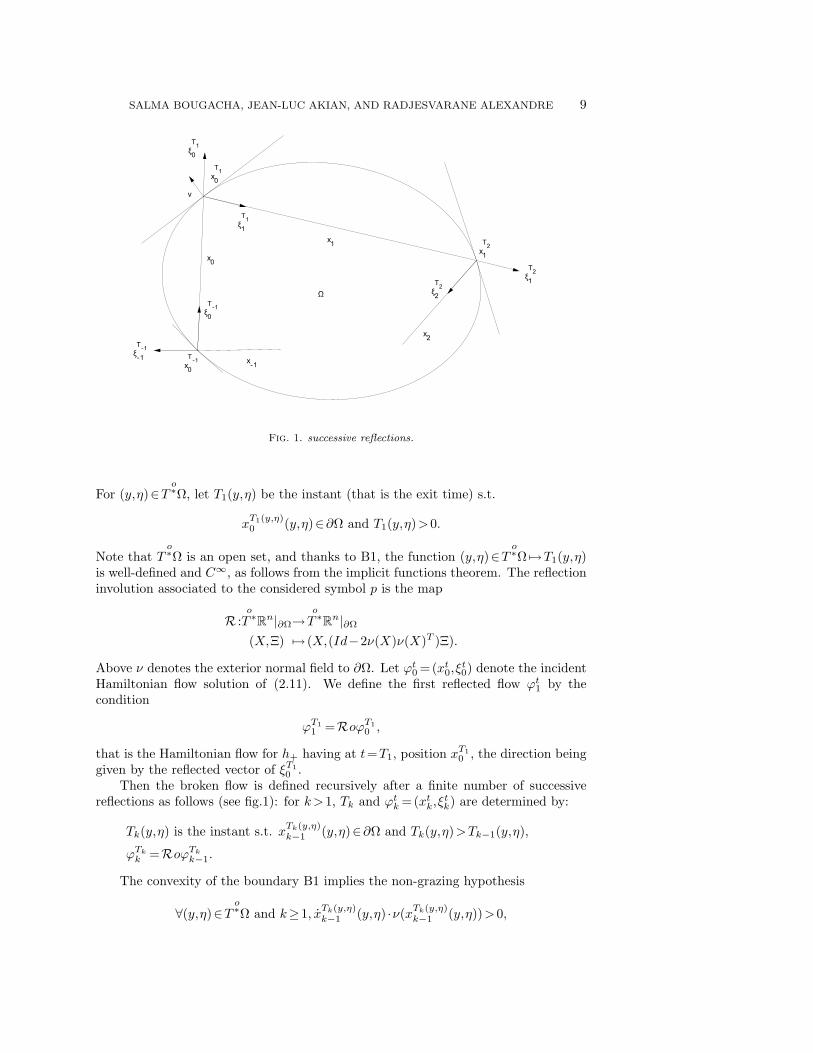
Fig. 1. successive reflections.

For (y,η)∈o

T ∗Ω, let T1(y,η) be the instant (that is the exit time) s.t.

xT1(y,η)0 (y,η)∈∂Ω and T1(y,η)>0.

Note thato

T ∗Ω is an open set, and thanks to B1, the function (y,η)∈o

T ∗Ω 7→T1(y,η)is well-defined and C∞, as follows from the implicit functions theorem. The reflectioninvolution associated to the considered symbol p is the map

R :o

T ∗Rn|∂Ω→o

T ∗Rn|∂Ω

(X,Ξ) 7→ (X,(Id−2ν(X)ν(X)T )Ξ).

Above ν denotes the exterior normal field to ∂Ω. Let ϕt0 = (xt0,ξt0) denote the incident

Hamiltonian flow solution of (2.11). We define the first reflected flow ϕt1 by thecondition

ϕT11 =RoϕT1

0 ,

that is the Hamiltonian flow for h+ having at t=T1, position xT10 , the direction being

given by the reflected vector of ξT10 .

Then the broken flow is defined recursively after a finite number of successivereflections as follows (see fig.1): for k>1, Tk and ϕtk = (xtk,ξ

tk) are determined by:

Tk(y,η) is the instant s.t. xTk(y,η)k−1 (y,η)∈∂Ω and Tk(y,η)>Tk−1(y,η),

ϕTkk =RoϕTkk−1.

The convexity of the boundary B1 implies the non-grazing hypothesis

∀(y,η)∈o

T ∗Ω and k≥1, xTk(y,η)k−1 (y,η) ·ν(xTk(y,η)

k−1 (y,η))>0,

10 GAUSSIAN BEAMS SUMMATION IN A CONVEX DOMAIN

where xtk−1 denotes ddtx

tk−1. Assumption B3 leads to

∀(y,η)∈o

T ∗Ω, Tk(y,η) →k→+∞

+∞. (2.14)

It insures that for a fixed point (y,η) ino

T ∗Ω, there is a finite number q+(y,η) ofreflections in [0,T ].

Following the method of Ralston in [36] p.220, we shall construct reflected beamsw1ε ,. ..,w

q+ε which satisfy the boundary estimate

∃m′>0 and s≥0 s.t. ‖B(w0ε + ·· ·+wq+ε )‖Hs([0,T ]×∂Ω) =O(εm

′),

together with the interior estimates

supt∈[0,T ]

‖Pwkε (t,.)‖L2(Ω) =O(εm), 1≤k≤ q+.

For each 1≤k≤ q+, the reflected beam wkε will be written as

wkε =eiψk/ε(ak0 + ·· ·+εNakN ).

To insure the interior estimates, each phase ψk and amplitudes akj (0≤ j≤N) mustsatisfy equations (2.6) and (2.9) on the reflected ray (t,xtk).As the beams vanish away from their associated rays, the contribution to the boundarynorm of w0

ε + ·· ·+wq+ε occurs when t is close to some Tk and then from the beams wk−1

ε

and wkε . The construction of the reflected beams is completed recursively. Assumethat the beam wk−1

ε has been constructed and that its associated phase satisfies

∂tψk−1(t,xtk−1) =−h+(xtk−1,ξtk−1), ∂xψk−1(t,xtk−1) = ξtk−1, (Pk−1.a)

ψk−1(t,xtk−1) is real, (Pk−1.b)

Im∂2xψk−1(t,xtk−1) is positive definite. (Pk−1.c)

One may write on the boundary ∂Ω

B(wk−1ε +wkε

)=(ε−mBdk−1

−mB + ·· ·+εNdk−1N

)eiψk−1/ε

+(ε−mBdk−mB + ·· ·+εNdkN

)eiψk/ε,

mB being the order of B (mB = 0 for Dirichlet and mB = 1 for Neumann).In order to satisfy the boundary estimate, the first step is to impose on ψk to

have the same time and tangential derivatives as ψk−1 at (Tk,xTkk−1), up to the orderR. More precisely, let us introduce boundary coordinates near xTkk−1 =xTkk as follows.We partition ∂Ω with a finite number of small open subsets U1,. ..,UL s.t. there existC∞ parametrizations

σl :Nl→Rn, l= 1,. ..,L,

where Nl are open subsets of Rn−1, σl(Nl) =Ul and σl a diffeomorphism from Nl toUl. Suppose that xTkk−1 belongs to Ul0 and denote xTkk−1 =σl0(zk). For x∈Rn close toxTkk−1, we may write

x=σl0(v)+vnν(σl0(v)),

SALMA BOUGACHA, JEAN-LUC AKIAN, AND RADJESVARANE ALEXANDRE 11

with v∈Nl0 and vn∈R. If we use the notation

σf(t,v,vn) =f(t,x),

then we impose

∂αt,vσψk(Tk, zk,0) =∂αt,v

σψk−1(Tk, zk,0), |α|≤R. (2.15)

Order 0 of (2.15) gives a real value for ψk(Tk,xTkk−1). Order 1 of this same constraintand order 0 of the eikonal equation (2.6) on ψk are both satisfied by setting

∂tψk(t,xtk) =−h+(xtk,ξtk), ∂xψk(t,xtk) = ξtk. (Pk.a)

It follows that

ψk(t,xtk) is real. (Pk.b)

Due to the non-grazing hypothesis, (2.15) and the compatibility condition result-ing from order 1 of the eikonal equation (2.6) provide with ∂2

xψk(Tk,xTkk−1). To solvethe Riccati equation on ∂2

xψk(t,xtk) with its given value at t=Tk, we need to studythe imaginary part of ∂2

xψk(Tk,xTkk−1). For k′=k−1,k, one has

∂t∂vσψk′(t,v,0) =Dσl0(v)T∂t∂xψk′(t,xtk′),

and

∂2vσψk′(t,v,0) =D2σl0(v)

(∂xψk′(t,xtk′)

)+Dσl0(v)T∂2

xψk′(t,xtk′)Dσl0(v).

Differentiating (Pk−1.a) and (Pk.a) yields

Im∂t∂xψk′(t,xtk′) =−Im∂2xψk′(t,x

tk′)x

tk′

and

Im∂2t ψk′(t,x

tk′) = xtk′ · Im∂2

xψk′(t,xtk′)x

tk′ .

Denote

Mk =∂2t,v

σψk−1(Tk, zk,0) =∂2t,v

σψk(Tk, zk,0). (2.16)

One has therefore

ImMk =(−xTkk′ , Dσl0(zk)

)TIm∂2

xψk′(Tk,xTkk−1)

(−xTkk′ , Dσl0(zk)

).

The non-grazing hypothesis insures that the matrices(−xTkk′ , Dσl0(zk)

)are non sin-

gular. Since Im∂2xψk−1(Tk,xTkk−1) is positive definite by (Pk−1.c), it follows that the

same property holds true for ImMk and consequently for Im∂2xψk(Tk,xTkk−1). Hence,

the matrix ∂2xψk(t,xtk) solution of a Riccati equation with its given value at t=Tk

satisfies

Im∂2xψk(t,xtk) is positive definite. (Pk.c)

12 GAUSSIAN BEAMS SUMMATION IN A CONVEX DOMAIN

Higher order derivatives of the reflected phase on the associated ray are deter-mined recursively. For 3≤ r≤R, ∂rxψk(t,xtk) satisfies linear ODEs with a given valueat t=Tk.

The second step is to prescribe that dk−1−mB+j+dk−mB+j vanish up to the order

R−2j−2 at (Tk,xTkk−1). These requirements provide with the derivatives of akj upto the order R−2j−2 at (Tk,xTkk−1). Hence, for 0≤ r≤R−2j−2, ∂rxa

kj (t,xtk) satisfy

linear systems of ODEs with initial conditions given at t=Tk.It follows from this construction that the choice of the (truncated up to fixed

orders) Taylor series of the phase and the amplitudes of the incident beam on thestarting point of the ray determines recursively the (truncated up to fixed orders)Taylor series of successively reflected beams’ phases and amplitudes.

Finally, the amplitudes akj are multiplied by a cutoff equal to 1 near xtk. Thereflected phases and amplitudes have the same forms as the incident ones

ψk(t,x) =∑|α|≤R

1α!

(x−xtk)α∂αxψk(t,xtk),

and

akj (t,x) =χd(x−xtk)∑

|α|≤R−2j−2

1α!

(x−xtk)α∂αx akj (t,xtk), j= 1,. ..,N.

2.2.2. Construction of beams associated to p−For the symbol p−, the same construction applies for the associated incident andreflected beams.

An incident beam for p− is a beam concentrated on the ray (t,x−t0 ), so it is

simply w0ε(−t,x). In fact, denoting Pw0

ε =N+2∑j=0

εj−2c0jeiψ0/ε, one can notice that

P [w0ε(−t,x)] = [Pw0

ε ](−t,x), and the amplitudes c0j (−t,x) vanish on x=x−t0 up tothe required orders.

Reflected beams for p− are obtained by reflecting ϕt0 backwards. For (y,η)∈o

T ∗Ω,let T−1(y,η)<0 be the instant s.t. x

T−1(y,η)0 (y,η) strikes the boundary ∂Ω. Denote

by ϕt−1 the Hamiltonian flow for h+ determined by the condition (see fig.1)

ϕT−1−1 =RoϕT−1

0 .

For k>1, one can define recursively the instants of reflections T−k and the Hamil-tonians flows ϕt−k for h+ as follows:

T−k(y,η) is the instant s.t. xT−k(y,η)−k+1 (y,η)∈∂Ω and T−k(y,η)<T−k+1(y,η),

ϕT−k−k =RoϕT−k−k+1.

Assumption B3 implies that Tk(y,η)→−∞ when k goes to −∞, and thus insuresa finite number q−(y,η) of reflections in [−T,0].

Then we build Gaussian beams w−kε for p− after 1≤k≤ q− backwards reflections,by imposing ‖B(w0

ε + ·· ·+w−q−ε )‖Hs([−T,0]×∂Ω) =O(εm

′) for some m′>0 and s≥0.

We write these beams as

w−kε =eiψ−k/ε(a−k0 + ·· ·+εNa−kN ).

SALMA BOUGACHA, JEAN-LUC AKIAN, AND RADJESVARANE ALEXANDRE 13

In particular, for 1≤k≤ q−, the phase ψ−k satisfies the following properties

∂tψ−k(t,xt−k) =−h+(xt−k,ξt−k), ∂xψ−k(t,xt−k) = ξt−k, (P−k.a)

ψ−k(t,xt−k) is real, (P−k.b)

Im∂2xψ−k(t,xt−k) is positive definite. (P−k.c)

Noting that (t,xt−k), k= 1,. ..,q−, are successively reflected rays for p−, the reflectedbeam of p− after k reflections is simply w−kε (−t,x).

2.2.3. Error estimates for individual Gaussian beamsWe fix (y,η)∈

o

T ∗Ω and choose d sufficiently small s.t. for k= 0,. ..,q±, t∈ [0,T ] and|x−x±t±k|≤d,

Imψ±k(±t,x)≥ const(x−x±t±k)2. (2.17)

One can see that this choice is always possible by the properties (Pk.a)-(Pk.b)-(Pk.c)of each phase ψk, −q−≤k≤ q+.

For t∈ [0,T ] and x∈Rn, let

w+ε (t,x) =

q+∑k=0

wkε (t,x) and w−ε (t,x) =q−∑k=0

w−kε (−t,x). (2.18)

Then we have the following estimates on these constructed beams.Lemma 2.2.

1. ‖ε−n4 +1w±ε (t,.)‖H1(Ω) .1 and ‖ε−n4 +1∂tw±ε (t,.)‖L2(Ω) .1 uniformly w.r.t. t∈

[0,T ],2. ‖P

(ε−

n4 +1w±ε

)(t,.)‖L2(Ω) .ε

R−12 uniformly w.r.t. t∈ [0,T ],

3. ‖B(ε−

n4 +1w±ε

)‖Hs([0,T ]×∂Ω) .ε−mB−s+

R+12 , s≥0.

The proof of this Lemma and other results rely on this standard estimate for p∈N

|x|pe−x2/εdx.ε

p2 e−x

2/(2ε),∀x∈Rn. (2.19)

For more details, we refer the interested reader to [36] or [30].

2.3. Gaussian beams summationThe constructed functions ε−

n4 +1w±ε are approximate solutions for the IBVP of the

wave equation with initial data

ε−n4 +1w±ε |t=0 =ε−

n4 +1

N∑j=0

εja0j |t=0e

iψ0|t=0/ε+ε−n4 +1

q±∑k=1

w±kε |t=0,

and

∂t(ε−

n4 +1w±ε

)|t=0 =±ε−n4

N+1∑j=0

εjf0j eiψ0|t=0/ε±ε−n4 +1

q±∑k=1

∂tw±kε |t=0,

where the f0j are related to the phase and amplitudes of w0

ε . One can show thatthe assumptions B1-B2 imply that x0

k /∈ Ω for k 6= 0. The exponential decrease of thephases away from their associated rays leads to

‖wkε |t=0‖H1(Ω) .ε∞ and ‖∂twkε |t=0‖L2(Ω) .ε∞, k 6= 0.

14 GAUSSIAN BEAMS SUMMATION IN A CONVEX DOMAIN

Modulo infinitely small remainders, the initial conditions of ε−n4 +1w±ε are thenε−n4 +1

N∑j=0

εja0j |t=0e

iψ0|t=0/ε,±ε−n4N+1∑j=0

εjf0j eiψ0|t=0/ε

.We wish to consider the IBVP (1.1) with general initial conditions (uIε,v

Iε ) in

H1(Ω)×L2(Ω). Note that ψ0|t=0 has properties similar to φ0, wherecnε− 3n

4 eiφ0(x,y,η)/ε denotes the kernel of T ∗ε , see formula (1.4) in the introduction. The

first step is to build, for a fixed point (y,η)∈o

T ∗Ω, asymptotic solutions with initialconditions close to (ε−

n4 +1eiφ0(.,y,η)/ε,0) and (0,ε−

n4 eiφ0(.,y,η)/ε) in H1(Ω)×L2(Ω).

Then one expects to fulfill more general initial data (uIε,vIε ) by decomposing uIε on

the family (ε−n4 +1eiφ0/ε)

(y,η)∈o

T∗Ωand vIε on the family (ε−

n4 eiφ0/ε)

(y,η)∈o

T∗Ω, indexed

by (y,η).Let us recover the notation of the beams referring to the starting points of the

incident flow. We fix (y,η)∈o

T ∗Ω and consider the incident beam w0ε(t,x,y,η) associ-

ated to the ray (t,xt0(y,η)) and the reflected beams w±kε (t,x,y,η), k= 1,. ..,q±. Taylorformulae (2.12) yields at t= 0

ψ0(0,x,y,η) =∑|α|≤R

1α!

(x−y)α∂αxψ0(0,y,y,η).

If one chooses the following initial spatial derivatives on the ray for the incident beam’sphase

ψ0(0,y,y,η) = 0,∂2xψ0(0,y,y,η) = iId and ∂αxψ0(0,y,y,η) = 0, 3≤|α|≤R,

then (P0.a) implies

ψ0(0,x,y,η) =η ·(x−y)+ i(x−y)2/2 =φ0(x,y,η). (2.20)

We assume henceforth that the incident beam’s phase satisfies (2.20). Consider anapproximate solution

12ε−

n4 +1(w+

ε +w−ε ).

Its initial data are ε−n4 +1N∑j=0

εja0j |t=0e

iφ0/ε,0

,with a redidue of order ε∞ in H1(Ω)×L2(Ω). To get the form (ε−

n4 +1eiφ0/ε,0), one

has to make a suitable choice for the amplitudes. The expansion (2.13) at t= 0 yields

a0j (0,x,y,η) =χd(x−y)

∑|α|≤R−2j−2

1α!

(x−y)α∂αx a0j (0,y,y,η), j= 0,. ..,N,

and one has full choice for the initial spatial derivatives of a0j on the ray up to the

order R−2j−2. Under the assumptions

a00(0,y,y,η) = 1, ∂αx a

00(0,y,y,η) = 0 for 1≤|α|≤R−2,

∂αx a0j (0,y,y,η) = 0 for |α|≤R−2j−2, 1≤ j≤N,

SALMA BOUGACHA, JEAN-LUC AKIAN, AND RADJESVARANE ALEXANDRE 15

one gets

N∑j=0

εja0j (0,x,y,η) =χd(x−y). (2.21)

Taking advantage of the exponential decrease of eiφ0(x,y,η)/ε for |x−y|≥d/2, onededuces that

‖ε−n4 +1N∑j=0

εja0j (0,.,y,η)eiφ0(.,y,η)/ε−ε−n4 +1eiφ0(.,y,η)/ε‖H1(Ω) .ε∞.

We keep the notations a0j and w0

ε to denote the amplitudes satisfying (2.21) andthe associated incident beam. For 1≤k≤ q±, we denote by w±kε the correspondingreflected beams and by w±ε the sum of the incident and reflected beams for p±.

Next, we shift to the initial condition on the time derivative, for which we con-struct a new incident beam w0

ε′ with amplitudes a0

j′. Indeed, an approximate solution

12ε−

n4 +1(w+

ε′−w−ε

′),

has initial data 0,ε−n4

N+1∑j=0

εj(i∂tψ0a

0j′+∂ta

0j−1′)|t=0e

iφ0/ε

,modulo a remainder of order ε∞ in H1(Ω)×L2(Ω), with a0

−1′=a0

N+1′= 0. In order to

approach the form (0,ε−n4 eiφ0/ε), we derive new initial Taylor series for the incident

beam’s amplitudes. As ∂tψ0(0,y,y,η) =−c(y)|η|, we impose

a00′(0,y,y,η) = i(c(y)|η|)−1

,∂αx

(∂tψ0a

00′)

(0,y,y,η) = 0 for 1≤|α|≤R−2,

∂αx

(i∂tψ0a

0j′+∂ta

0j−1′)

(0,y,y,η) = 0 for |α|≤R−2j−2, 1≤ j≤N.

One gets

N+1∑j=0

εj(i∂tψ0a

0j′+∂ta

0j−1′)

(0,x,y,η) = 1+N∑j=0

εj∑

|α|=R−2j−1

(x−y)αzα(x,y,η)

+εN+1∂ta0N′(0,x,y,η), (2.22)

where zα are smooth remainders that vanish for |x−y|≥d. Making use of (2.19) and(2.10), one can show that

‖ε−n4N+1∑j=0

εj(i∂tψ0a

0j′+∂ta

0j−1′)

(0,.,y,η)eiφ0(.,y,η)/ε−ε−n4 eiφ0(.,y,η)/ε‖L2(Ω) .εR−1

2 .

Let w±kε′, 1≤k≤ q±, be the reflected beams associated to w0

ε′ and denote by w±ε

′ thesum of the so obtained incident and reflected beams for p±. Hence, the approximatesolutions

12ε−

n4 +1(w+

ε +w−ε )(t,x,y,η) and12ε−

n4 +1(w+

ε′−w−ε

′)(t,x,y,η),

16 GAUSSIAN BEAMS SUMMATION IN A CONVEX DOMAIN

have the required initial data(ε−

n4 +1eiφ0(x,y,η)/ε,0

)and

(0,ε−

n4 eiφ0(x,y,η)/ε

),

modulo remainders of respective orders ε∞ and εR−1

2 in H1(Ω)×L2(Ω).To fulfill general initial conditions (uIε,v

Iε ), the previous computations together

with the identity T ∗ε Tε= Id, suggest that we look for an approximate solution such as

cn2ε−

3n4

∫o

T∗Ω

TεuIε(y,η)

(w+ε (t,x,y,η)+w−ε (t,x,y,η)

)dydη

+cn2ε−

3n4

∫o

T∗Ω

εTεvIε

(w+ε′(t,x,y,η)−w−ε

′(t,x,y,η))dydη.

Let us notice that it is not clear that the previous integral is well defined.Firstly, the construction of w±ε

(′)(t,x,y,η) breaks down when y approaches theboundary ∂Ω because the numbers of reflections in [0,±T ] become infinitely large.Next we need to tackle the problem of integration for large η.

One way to overcome these two problems is to require that the initial FBI trans-forms are compactly supported modulo small remainders. This requirement is in thespirit of considering only compactly supported symbols in the study of the FIOs of[24]. Nevertheless, this restriction was removed recently by Swart and Rousse in [40].In particular, a general boundedness result of FIOs with complex phases for sub-quadratic Hamiltonians was established therein. The proof is rather subtle and reliesin particular on Cotlar-Stein estimate. The same arguments can be used for the con-stant coefficient wave equation but seem not to work for the general wave equation.In fact, in this case, the second derivatives of the Hamiltonian are not bounded andthus the proof of [40] needs to be adapted.

A last problem related to the wave equation is the integration for small η.

In view of all these difficulties, this explains why we have made in the introductionthe assumptions A2 and A3 on the initial data, which we recall

uIε and vIε are supported in a fixed compact K⊂Ω,‖TεuIε‖L2(Rn×Rcη) =O(ε∞) and ‖TεvIε‖L2(Rn×Rcη) =O(ε∞),

where Rη =η∈Rn,r0≤|η|≤ r∞, 0<r0<r∞. These assumptions are satisfied for in-stance by a large class of WKB functions aeiΦ/ε, a∈C∞0 (Ω). Indeed the non-stationaryphase lemma implies that the FBI transform of such a function is of order O(ε∞) out-side the compact set

A×B=y∈Rn,dist(y,suppa)≤ c×η∈Rn,dist(η,∂xΦ(A))≤ c, c>0,

see Lemmas 4.2 and 4.3 of [39]. Thus aeiΦ/ε satisfies assumption A3, provided that∂xΦ does not vanish on suppa.Remark 2.3. Another strategy can be used to match initial conditions of WKB formin a Gaussian beams summation [28, 45]. It consists of integrating the beams asso-ciated to rays that start from y∈ suppa with the direction η=∂xΦ(y). The accuracyof such obtained solutions faces a damage caused by caustics, namely an extra factorε

1−n4 appears in the error estimate. This loss originates from the restriction to rays

x±t±k(y,∂xΦ(y)) (k= 0,. ..,N±), which technically leads to considering the deformation

SALMA BOUGACHA, JEAN-LUC AKIAN, AND RADJESVARANE ALEXANDRE 17

matrices ∂y[x±t±k(y,∂xΦ(y))] singular at caustics (see Lemma 5.1 of [28]). The summa-tion over rays starting with general directions η independent of y uses the symplecticmaps ϕ±t±k and thus provides a phase space description of the solution that unfolds thecaustics.

Let ρ be a cut-off of C∞0 (Rn, [0,1]) supported in a compact Ky⊂Ω and satisfying

ρ(y) = 1 if dist(y,K)<∆ for a small ∆>0, (2.23)

and φ a cut-off of C∞0 (Rn,[0,1]) supported in a compact Kη⊂Rn\0 s.t. φ= 1 onRη.

One can establish that the assumptions A2 and A3 imply

‖(1−ρ(y)φ(η))TεuIε‖L2y,η

.ε∞ and ‖(1−ρ(y)φ(η))TεvIε‖L2y,η

.ε∞.

In fact, viewing the FBI transform as the Fourier Transform of some auxiliary functionyields by Parseval equality the following resultLemma 2.4. Let a be a positive real and G a measurable subset of Rn s.t. dist(G,K)≥a. If u∈L2(Rnw) is supported in K then

‖1G(y)Tεu‖L2y,η

= cnε−n4 ‖1G(y)u(w)e−(w−y)2/(2ε)‖L2

w,y.e−a

2/(4ε)‖u‖L2w.

On the other hand, if (y,η) varies in Ky×Kη, then q+(y,η) is uniformly bounded.In fact, for j≥1, the Tj are positive, depend continuously on (y,η) and the property(2.14) insures that Tj+∞ when j→+∞. Thus they uniformly go to +∞ on thecompact Ky×Kη, by Dini’s theorem on the sequence (1/Tj)j≥1. As Tq+ ≤T , it followsthat sup

Ky×Kηq+<+∞. The same result holds true for q−. Denote N±= sup

Ky×Kηq±.

The construction of the reflected beams in section 2.2 may be continued up to N±reflections.

The final result of the discussion above is an approximate solution proposed as

uRε (t,x) =12ε−

3n4 cn

∫R2n

ρ(y)φ(η)[εTεv

Iε (y,η)(

N+∑k=0

wkε′(t,x,y,η)−

N−∑k=0

w−kε′(−t,x,y,η))

+TεuIε(y,η)(

N+∑k=0

wkε (t,x,y,η)+N−∑k=0

w−kε (−t,x,y,η))]dydη.

(2.24)

This approximate solution is indexed by R, the order of vanishing of the eikonalequation (2.6) on the ray. The incident beams’ phase fulfills the initial conditions(2.20) and their amplitudes satisfy respectively (2.21) for w0

ε and (2.22) for w0ε′ for

every (y,η)∈ suppρ⊗φ,. The size d∈]0,1] of the support of the cut-offs multiplyingthe amplitudes no longer depends on (y,η) and would be chosen sufficiently small tosatisfy various constraints we set out in the following section.

In the sequel, we prove that this family of functions (uRε ) indeed allows to approachthe exact solution of the IBVP problem (1.1) to any arbitrary power of ε by choosingthe order R. The difference between the asymptotic solutions and the exact oneis investigated in C([0,T ],H1(Ω))×C1([0,T ],L2(Ω)) by means of error estimates inthe interior equation, the boundary condition and the initial conditions. The onlyassumptions needed on the initial data are A1, A2 and A3.

18 GAUSSIAN BEAMS SUMMATION IN A CONVEX DOMAIN

3. Justification of the asymptoticsWe aim to estimate ‖uRε (t,.)−uε(t,.)‖H1(Ω) and ‖∂tuRε (t,.)−∂tuε(t,.)‖L2(Ω) fort∈ [0,T ].

It follows from standard results [7] that the IBVP for the wave equation is well-posed, and furthermore one has the energy estimate (as a consequence of [25] p.185for the Dirichlet problem and of [3] p.224 for the Neumann problem)

Supt∈[0,T ]

‖uRε (t,.)−uε(t,.)‖H1(Ω) + Supt∈[0,T ]

‖∂tuRε (t,.)−∂tuε(t,.)‖L2(Ω) .

Supt∈[0,T ]

‖PuRε ‖L2(Ω) +‖BuRε ‖Hs([0,T ]×∂Ω) (3.1)

+‖uRε (0,.)−uIε‖H1(Ω) +‖∂tuRε (0,.)−vIε‖L2(Ω),

where s= 1 for Dirichlet and s= 12 for Neumann.

The asymptotics will be proven by estimating each term of the r.h.s. of thisenergy estimate.

Since the error estimates in the interior and near the boundary use similar com-putations, a unified framework will be used by considering the more general problemof estimates linked with a suitable family of approximation operators Oα in section3.1. Then in section 3.2 we use these estimates for the interior term ‖PuRε ‖L2(Ω) in3.2.1, the boundary term ‖BuRε ‖Hs([0,T ]×∂Ω) in 3.2.2 and the initial conditions errorsin 3.2.3. All these estimates are gathered in section 3.3 to prove Theorem 1.1.

3.1. Approximation operatorsLet Kz,θ be a compact of R2n and

Er =(x,z,θ)∈Rn×Kz,θ, |x−z|≤ r, r>0.

Consider a complex phase function Φ smooth on an open set containing Er0 for somer0∈]0,1]. We assume, for (z,θ)∈Kz,θ ,that

∂xΦ(z,z,θ) =θ,Φ(z,z,θ) is real,∂2xΦ(z,z,θ) has a positive definite imaginary part.

(Q1)

Taylor expansion of Φ together with assumptions (Q1) imply the existence of someconstant r[Φ]∈]0,r0] s.t. for (x,z,θ)∈Er[φ]

ImΦ(x,z,θ)≥ const(x−z)2.

Consider a sequence lε∈C∞(Rnx×R2nz,θ,C). We assume that

lε(x,z,θ) = 0 if (x,z,θ) /∈Er[Φ],lε is uniformly bounded in L∞(R3n). (Q2)

For a given multi-index α, let the operators O0 (lε,Φ/ε) and Oα (lε,Φ/ε) be given by[O0 (lε,Φ/ε)h

](x) =

∫R2n

h(z,θ)lε(x,z,θ)eiΦ(x,z,θ)/εdzdθ, h∈L2(R2n),

and

[Oα (lε,Φ/ε)h](x) =∫

R2nh(z,θ)lε(x,z,θ)(x−z)αeiΦ(x,z,θ)/εdzdθ, h∈L2(R2n),

SALMA BOUGACHA, JEAN-LUC AKIAN, AND RADJESVARANE ALEXANDRE 19

with x∈Rn.Let us show that these are operators from L2(R2n) to L2(Rn). For x∈Rn we

have ∫|lεeiΦ/ε|dzdθ.

∫(z,θ)∈Kz,θ

e−const(x−z)2/εdzdθ,

and thus ∫|lεeiΦ/ε|dzdθ.ε

n2 .

Similarly, for (z,θ)∈Kz,θ ∫|lεeiΦ/ε|dx.ε

n2 .

It is then immediate by Schur’s lemma, that

‖O0 (lε,Φ/ε)‖L2(R2n)→L2(Rn) .εn2 .

Similar arguments lead to the estimate

‖Oα (lε,Φ/ε)‖L2(R2n)→L2(Rn) .εn2 +|α|2 .

However, the use of the module inside the previous integrals makes one lose the highlyoscillatory character of eiΦ/ε, that is the contribution of eiθ·(x−z)/ε. In fact, a betterestimate on the norms of these operators is available if a precise control on lε isassumed. This is stated in the following lemmaLemma 3.1. Assume that ε

k2 ∂kxb lε (b= 1,. ..,n) is uniformly bounded in L∞(R3n), at

any order k∈N. Then, one has1. ‖O0 (lε,Φ/ε)‖L2(R2n)→L2(Rn) .ε

3n4 ,

2. ‖Oα (lε,Φ/ε)‖L2(R2n)→L2(Rn) .ε3n4 +

|α|2 .

Proof. 1. Let h∈L2(R2n). We shall use the notations f(x) for f(x,z,θ) and f ′(x)for f(x,z′,θ′). First of all, we explicit the L2 norm of O0 (lε,Φ/ε)h as

‖O0 (lε,Φ/ε)h‖2L2 =∫

R4nhh′eiΦ(z)/ε−iΦ′(z′)/εei(θ

′.z′−θ.z)/ε (3.2)[∫Rnlε(x)l

′ε(x)ei(θ−θ

′).x/εeiΘ(x,z,θ,z′,θ′)/εdx]dzdz′dθdθ′,

where

Θ(x,z,θ,z′,θ′) =∑|α|=2

(x−z)α∫ 1

02α! (1−s)∂

αxΦ(z+s(x−z),z,θ)ds

−∑|α|=2

(x−z′)α∫ 1

02α! (1−s)∂

αxΦ(z′+s(x−z′),z′,θ′)ds.

Let Iε denote the integral inside the brackets, that we begin to estimate. For 1≤ b≤nand K ∈N, successive integrations by parts give

Iε(z,z′,θ,θ′)iKε−K(θb−θ′b)K =

(−1)K∑

N+N ′=K

(KN

)∫Rnei(θ−θ

′).x/ε∂Nxb [eiΘ/ε]∂N

′

xb[lεl′ε]dx,

20 GAUSSIAN BEAMS SUMMATION IN A CONVEX DOMAIN

where(KN

)denotes the standard binomial coefficient. To estimate ∂Nxb [e

iΘ/ε], N ∈N,

we use the following result, of which proof is postponed to the end of this sectionLemma 3.2. Let p∈N∗ and consider a complex phase function Fp of the form

Fp(x,z) =∑|α|=p

(x−z)αfα(x,z),

with fα smooth on some open set of R2n containing a subset S and ∂kxfα bounded onS for any k≥0.Then for (x,z)∈S, |x−z|≤1, small ε, N ∈N and b= 1,. ..,n, one has

|∂Nxb [eiFp/ε]|≤ max

|α|=p0≤s≤N1≤k≤N

(supS|∂sxbfα|

)k( ∑Np ≤k≤N

ε−k|x−z|kp−N +∑

1≤k<Np

ε−N/p)|eiFp/ε|.

We write Θ =F2− F ′2 with

F2(x,z,θ) =∑|α|=2

(x−z)α∫ 1

0

2α!

(1−s)∂αxΦ(z+s(x−z),z,θ)ds,

for (x,z,θ)∈Er[Φ]. By Leibnitz formula, ∂Nxb [eiΘ/ε] is a sum of terms of the form

∂N1xb

[eiF2/ε]∂N2xb

[e−iF′2/ε], 0≤N1,N2≤N,N1 +N2 =N.

Note that ImF2 = ImΦ. Lemma 3.2 yields for N1∈N and (x,z,θ)∈Er[Φ]

|∂N1xb

[eiF2/ε]|.

∑N12 ≤k≤N1

ε−k|x−z|2k−N1 +ε−N1/2

e−const(x−z)2/ε.

Hence

|∂N1xb

[eiF2/ε]|.ε−N12 e−const(x−z)2/ε.

A similar estimate may be obtained for |∂N2xb

[eiF′2/ε]| when (x,z′,θ′)∈Er[Φ]. It follows,

for (x,z,θ),(x,z′,θ′)∈Er[Φ], that

|∂N1xb

[eiF2/ε]∂N2xb

[e−iF′2/ε]|.ε−

N1+N22 e−const(x−z)2/εe−const(x−z′)2/ε,

and thus

|∂Nxb [eiΘ/ε]|.ε−

N2 e−const(2x−z−z′)2/εe−const(z−z′)2/ε, N ∈N.

Since εN′2 ∂N

′

xb[lε l′ε], N

′∈N, is uniformly bounded

|∂Nxb [eiΘ/ε]∂N

′

xb[lεl′ε]|.ε−

N+N′2 e−const(2x−z−z′)2/εe−const(z−z′)2/ε,

and we deduce that

|Iε(z,z′,θ,θ′)(θb−θ′b√

ε

)K|.ε

n2 e−const(z−z′)2/ε,

SALMA BOUGACHA, JEAN-LUC AKIAN, AND RADJESVARANE ALEXANDRE 21

for b= 1,. ..,n and K ∈N.Choosing K>n and coming back to (3.2) gives

‖O0 (lε,Φ/ε)h‖2L2 .εn2

∫R4n|h||h′|e−const(z−z′)2/εdzdz′(1+(θ−θ′)2/ε)−

K2 dθdθ′.

Upon using the change of variables:

(z,z′) = (u+√εv,u−

√εv) and (θ,θ′) = (σ+

√εδ,σ−

√εδ),

we have

‖O0 (lε,Φ/ε)h‖2L2 .ε3n2

∫R2n

∫R2n|h(u+

√εv,σ+

√εδ)||h(u−

√εv,σ−

√εδ)|dudσ

e−constv2(1+4δ2)−K2 dvdδ,

from which, using Cauchy-Schwartz inequality for the first integral, we get

‖O0 (lε,Φ/ε)h‖2L2 .ε3n2 ‖h‖2L2 .

2. Arguments are similar to the previous case. For a multi-index α, we have

‖Oα (lε,Φ/ε)h‖2L2 =∫

R4nhh′eiΦ(z)/ε−iΦ′(z′)/εei(θ

′.z′−θ.z)/ε

Iαε (z,z′,θ,θ′)dzdz′dθdθ′,

where, for b= 1,. ..,n and K ∈N

Iαε (z,z′,θ,θ′)iKε−K(θb−θ′b)K = (−1)K∑

N+N ′=K

(KN

)∫Rnei(θ−θ

′).x/ε

∂Nxb [(x−z)α(x−z′)αeiΘ/ε]∂N

′

xb[lεl′ε]dx.

We note that ∂Nxb [(x−z)α(x−z′)αeiΘ/ε] is a finite sum of terms of the form

(x−z)α−keb

(x−z′)α−leb

∂mxb [eiΘ/ε],

where k,l≤αb, k+ l+m=N and eb denotes the vector of Rn s.t. eba= δab.For (x,z,θ),(x,z′,θ′)∈Er[Φ], it follows that

|∂Nxb [(x−z)α(x−z′)αeiΘ/ε]|.ε|α|−

N2 e−const(2x−z−z′)2/εe−const(z−z′)2/ε.

Since εN′2 ∂N

′

xb[lεl′ε] is uniformly bounded

|∂Nxb [(x−z)α(x−z′)αeiΘ/ε]∂N

′

xb[lεl′ε]|.

ε|α|−N+N′

2 e−const(2x−z−z′)2/εe−const(z−z′)2/ε,

and thus

|Iαε (z,z′,θ,θ′)(θb−θ′b√

ε

)K|.ε

n2 +|α|e−const(z−z′)2/ε,

22 GAUSSIAN BEAMS SUMMATION IN A CONVEX DOMAIN

and finally

‖Oα (lε,Φ/ε)h‖2L2 .ε3n2 +|α|‖h‖2L2 .

Similar computations can be carried out for a phase Φ and a sequence of ampli-tudes lε that depend on a parameter m∈ [0,M ]. In this case, we consider for m∈ [0,M ]a compact Kz,θ(m)⊂R2n and denote for r>0

Er =(m,x,z,θ)∈ [0,M ]×R3n, (z,θ)∈Kz,θ(m), |x−z|≤ r.

We are interested in a phase function Φ smooth on an open set containing Er0 forsome r0∈]0,1]. We make the further assumption

Er0 is compact,

which is obviously fulfilled when no parameter m interferes. Assuming, for m∈ [0,M ]and (z,θ)∈Kz,θ(m), that

∂xΦ(m,z,z,θ) =θ,Φ(m,z,z,θ) is real,∂2xΦ(m,z,z,θ) has a positive definite imaginary part,

(Q1’)

one can find r[Φ]∈]0,r0] s.t. for (m,x,z,θ)∈Er[φ]

ImΦ(m,x,z,θ)≥ const(x−z)2.

Similarly, the sequence lε will be assumed to belong to C∞([0,M ]×Rnx×R2nz,θ,C) and

to satisfy

for m∈ [0,M ], lε(m,x,z,θ) = 0 if (m,x,z,θ) /∈Er[Φ],lε is uniformly bounded in L∞([0,M ]×R3n). (Q2’)

One can then define, for every given m∈ [0,M ] and α multiindex (|α|≥0), the oper-ators Oα (lε(m,.),Φ(m,.)/ε), for which the following estimate may be establishedLemma 3.3. Assume that ε

k2 ∂kxb lε (b= 1,. ..,n) is uniformly bounded in

L∞([0,M ]×R3n), at any order k∈N. Then, one has

‖Oα (lε(m,.),Φ(m,.)/ε)‖L2(R2n)→L2(Rn) .ε3n4 +

|α|2 , uniformly w.r.t. m∈ [0,M ].

In fact, all the estimates used in the proof of Lemma 3.1 hold true with a parameterm∈ [0,M ], since Er[φ] is still compact, owing to the compactness of Er0 .

We now give the proof of Lemma 3.2. Using the formula of composite functions’high derivatives (see, e.g., [11] p.161), the N th partial derivative of eiFp/ε is

∂Nxb [eiFp/ε] =

N∑k=1

(i

ε

)k ∏j1+···+jk=N

j1,...,jk≥1

N !k!j1! .. .jk!

∂j1

xbFp .. .∂

jk

xbFpe

iFp/ε, N ∈N∗.

Each derivative ∂jxbFp is a linear combination of

(x−z)α+(s−j)eb∂sxbfα, |α|=p,0≤s≤ j and αb≥ j−s.

SALMA BOUGACHA, JEAN-LUC AKIAN, AND RADJESVARANE ALEXANDRE 23

The product ∂j1

xbFp .. .∂

jk

xbFp is then a linear combination of

(x−z)α1+(s1−j1)eb+···+αk+(sk−jk)eb∂s

1

xbfα1 .. .∂s

k

xbfαk ,

where for i= 1,. ..,k, |αi|=p, 0≤si≤ ji and αib≥ ji−si. As j1 + ·· ·+jk =N , then forN/p≤k≤N and |x−z|≤1 one has

|(x−z)α1+(s1−j1)eb+···+αk+(sk−jk)eb |≤ |x−z|kp−N .

Thus for N ∈N∗, (x,z)∈S, |x−z|≤1 and small ε

|∂Nxb [eiFp/ε]|≤ max

|α|=p0≤s≤N1≤k≤N

(supS|∂sxbfα|

)k( ∑Np ≤k≤N

ε−k|x−z|kp−N +∑

1≤k<Np

ε−N/p)|eiFp/ε|,

which of course is also valid for N = 0.

3.2. Error estimatesThe different terms of the energy estimate (3.1) will be estimated separately. Ourmain interest is to prove that the interior and boundary errors given for individualbeams in Lemma 2.2 hold true for an infinite sum of beams, when the starting pointsof the incident flow vary in the compact Ky×Kη. The control we have is that we canmake the Gaussian beams vanish outside the very neighbourhood of their associatedrays, by making the parameter d as small as needed.

3.2.1. The interior estimate of PuRεIn this section, we will prove that

Supt∈[0,T ]

‖PuRε (t,.)‖L2(Ω) .εR−1

2 .

For 0≤k≤N+, one has by construction

Pwkε =N+2∑j=0

εj−2ckj eiψk/ε,

where ckj is null on (t,xtk), up to the order R−2j, for j= 0,. ..,N+1. One may write

Pwkε (t,x) =N+1∑j=0

εj−2( ∑|α|=R−2j+1

(x−xtk)αrkα(t,x)eiψk(t,x)/ε)

+εNckN+2(t,x)eiψk(t,x)/ε,

where rkα denotes the remainder in the Taylor formulae of ckj near xtk. Applying P to(2.24) gives then terms of the form

pj,kε (t,x) =ε−3n4 −1+j

∑|α|=R−2j+1

∫R2n

ρ(y)φ(η)hε(y,η)

(x−xtk)αrkα(t,x,y,η)eiψk(t,x,y,η)/εdydη,

with j= 0,. ..,N+1, and

pN+2,kε (t,x) =ε−

3n4 +N+1

∫R2n

ρ(y)φ(η)hε(y,η)ckN+2(t,x,y,η)eiψk(t,x,y,η)/εdydη,

24 GAUSSIAN BEAMS SUMMATION IN A CONVEX DOMAIN

where hε is either ε−1TεuIε or TεvIε and 0≤k≤N+. Other terms of the same form

come from Pwkε′, 0≤k≤N+, and P [w−k(′)

ε (−t,.)], 0≤k≤N−.Let f(t,x,z,θ) =f(t,x,ϕtk−1(z,θ)). Using the volume preserving change of vari-

ables (z,θ) =ϕtk(y,η) in the definition of pj,kε (t,x), 0≤ j≤N+1, writes it as a sum ofterms of the form

ε−3n4 −1+j

∫R2n

ρ⊗φ(t,z,θ)hε(t,z,θ)(x−z)αrkα(t,x,z,θ)eiψk(t,x,z,θ)/εdzdθ,

with |α|=R−2j+1. Similarly, pN+2,kε (t,x) is a sum of terms of the form

ε−3n4 +N+1

∫R2n

ρ⊗φ(t,z,θ)hε(t,z,θ)ckN+2(t,x,z,θ)eiψk(t,x,z,θ)/εdzdθ.

We want to estimate these integrals with the help of the operators Oα applied to1

supp ρ⊗φ(t,.)hε. Clearly 1

supp ρ⊗φ(t,.)TεvIε (t,.) is uniformly bounded (w.r.t. ε and t)

in L2(R2n). But more work is needed for estimating ε−11supp ρ⊗φ(t,.)

TεuIε(t,.), whichis given in the following resultLemma 3.4. ‖ε−1Tεu

Iε‖L2(R2n) .1.

Proof. Differentiating (1.3) w.r.t. yb, 1≤ b≤n, yields

ε12 ∂yb(Tεu

Iε) = iηbε

− 12Tεu

Iε−cnε−

3n4

∫RnuIε(w)ε−

12 (yb−wb)eiη.(y−w)/ε−(y−w)2/(2ε)dw.

The l.h.s. is bounded in L2y,η because ∂yb(Tεu

Iε) =Tε(∂wbu

Iε). The second term of the

r.h.s. is the Fourier transform of a bounded function in L2w, thus it can be estimated

using Parseval equality. One gets

‖ε− 3n4

∫RnuIε(w)ε−

12 (yb−wb)eiη.(y−w)/ε−(y−w)2/(2ε)dw‖L2

y,η.‖uIε‖L2

w.

Thus ‖ε− 12 ηbTεu

Iε‖L2

y,η.1 and consequently ‖ε− 1

2φ(η)TεuIε‖L2y,η

.1. Assumption A3yields

‖ε− 12Tεu

Iε‖L2

y,η.1.

Hence ‖uIε‖L2 .√ε. Reproducing the same arguments on the following equality

∂yb(TεuIε) = iηbε

−1TεuIε−cnε−

3n4

∫Rn

(ε−

12uIε

)(w)ε−

12 (yb−wb)e

iεη.(y−w)− 1

2ε (y−w)2dw,

leads to ‖uIε‖L2 .ε.Let us now check if a family of operators Oα may be used. First, each phase ψk

is smooth on an open set containing

E1 =(t,x,z,θ)∈ [0,T ]×R3n,(z,θ)∈ϕtk(Ky×Kη), |x−z|≤1.

E1 is compact, since the map (t,y,η) 7→ (t,ϕtk(y,η)) is continuous. For t∈ [0,T ] and(z,θ)∈ϕtk(Ky×Kη), one has by (Pk.a), (Pk.b) and (Pk.c)

∂xψk(t,z,z,θ) = ξtk(z,θ) =θ,

ψk(t,z,z,θ) is real,∂2xψk(t,z,z,θ) has a positive definite imaginary part.

SALMA BOUGACHA, JEAN-LUC AKIAN, AND RADJESVARANE ALEXANDRE 25

Hence ψk satisfies properties (Q1’). We fix some r[ψk]∈]0,1] so that

Imψk(t,x,z,θ)≥ const(x−z)2 for every (t,x,z,θ)∈Er[ψk]. (3.3)

Next, for R−2N−1≤|α|≤R+1, let

lα,k(t,x,z,θ) = ρ⊗φ(t,z,θ)rkα(t,x,z,θ), t∈ [0,T ],

and

l0,k(t,x,z,θ) = ρ⊗φ(t,z,θ)ckN+2(t,x,z,θ), t∈ [0,T ].

Then the lα,k, |α|=R−2N−1,. ..,R+1, and l0,k are smooth w.r.t. all their variables.Assume that

d≤ r[ψk], k= 0,. ..,N+. (3.4)

Because of the cut-offs χd in the beams’ amplitudes, it follows thatckN+2(t,x,z,θ) = rkα(t,x,z,θ) = 0 if |x−z|≥ r[ψk]. Furthermore, ρ⊗φ(t,z,θ) = 0 for(z,θ) /∈ϕtk(Ky×Kη). The lα,k satisfy therefore assumptions (Q2’).

It follows that the operators Oα can be used to obtain for t∈ [0,T ] and x∈Rn

pj,kε (t,x) =ε−3n4 −1+j

∑|α|=R−2j+1

[Oα(lα,k(t,.),ψk(t,.)/ε

)1

supp ρ⊗φ(t,.)hε(t,.)

](x),

with j= 0,. ..N+1, and

pN+2,kε (t,x) =ε−

3n4 +N+1

[O0(l0,k(t,.),ψk(t,.)/ε

)1

supp ρ⊗φ(t,.)hε(t,.)

](x).

Applying Lemma 3.3 and making use of (2.10) yields

‖pj,kε (t,.)‖L2(Ω) .εR−1

2 , uniformly w.r.t. t∈ [0,T ], for j= 0,. ..,N+2.

3.2.2. The boundary estimate of BuRεWe will now estimate BuRε |∂Ω, B=D or N standing for Dirichlet and Neumannoperators respectively. We shall prove that

‖DuRε ‖H1([0,T ]×∂Ω) .εR−1

2 and ‖NuRε ‖H1/2([0,T ]×∂Ω) .εR−2

2 . (3.5)

To this end, we note that the boundary operator B applied to (2.24) is a sum of termsarising from Bwkε , 0≤k≤N+ such as

bjε(t,x) =ε−3n4 +1−mB+j

∫R2n

ρ(y)φ(η)hε(y,η)N+∑k=0

dk−mB+j(t,x′,y,η)eiψk(t,x′,y,η)/εdydη,

(3.6)

with j= 0,. ..,N+mB , and others with the same form arising from Bwkε′, 0≤k≤N+,

and B[w−k(′)ε (−t,.)], 0≤k≤N−.

Above and as in the previous section, hε is either ε−1TεuIε or TεvIε and thus is

uniformly bounded in L2.We first study the support of the amplitudes. Next we use local boundary coor-

dinates to expand the boundary phases and introduce a change of variables on (y,η)that makes the obtained phases satisfy properties (Q1). The previous results on theapproximation operators Oα are then used to estimate the boundary norms.

26 GAUSSIAN BEAMS SUMMATION IN A CONVEX DOMAIN

Support of the amplitudesDue to assumptions B1-B2-B3, the rays stay away from the boundary except fortimes near the instants of reflections. For (y,η)∈Ky×Kη and t∈ [0,T ] near someTk(y,η), 0≤k≤N+ , only xtk(y,η) and, if k 6= 0, xtk−1(y,η) approach the boundary.This suggests that the meaningful contributions to the boundary norm of bjε arethe quantities dk−1

−mB+j(.,y,η)eiψk−1(.,y,η)/ε+dk−mB+j(.,y,η)eiψk(.,y,η)/ε near Tk(y,η),k= 1,. ..,N+. Furthermore, for t in the neighbourhood of Tk(y,η) and x′∈∂Ω, oneexpects dk−1

−mB+j(t,x′,y,η) and dk−mB+j(t,x

′,y,η) to vanish away from xTk(y,η)k−1 (y,η),

because of the cut-offs in the amplitudes. In the remainder, we show that these twointuitive points are true. The key argument is that (t,y,η) vary in a compact set.

The first point is rather easy to see. For (y,η)∈Ky×Kη, let us considera period smaller than any lapse of time between two successive reflections, sayβ(y,η) = min

0≤k≤N+(Tk(y,η)−Tk−1(y,η))/3, (T0 = 0), and define the intervals

I0(y,η) =∅, Ik(y,η) = [Tk(y,η)−β(y,η),Tk(y,η)+β(y,η)] for k= 1,. ..,N+,

and IN++1(y,η) =∅.

For each k= 0,. ..,N+, let

Ak =(t,y,η)∈ [0,T ]×Ky×Kη, t /∈o

Ik(y,η)∪o

Ik+1(y,η).

For (t,y,η)∈Ak, dist(xtk(y,η),∂Ω)>0 and has then a positive lower bound by conti-nuity on the compact Ak. One has by (3.3) and (3.4)

ψk(t,x,y,η)≥ const(x−xtk(y,η))2,

for (t,x,y,η)∈ [0,T ]×Rn×Ky×Kη s.t. |x−xtk(y,η)|≤d. Thus

|dk−mB+j(t,x′,y,η)eiψk(t,x′,y,η)/ε|≤e−const/ε for (t,y,η)∈Ak and x′∈∂Ω.

All we have to care about is then the contribution to the norm at the boundary ofdk−1−mB+je

iψk−1/ε and dk−mB+jeiψk/ε at times in the interval Ik, k= 1,. ..,N+. Let

qj,kε =ε−3n4 +1−mB+j

∫R2n

ρ⊗φhε1Ik(t)(dk−1−mB+je

iψk−1/ε

+dk−mB+jeiψk/ε)dydη.

Summing over k= 1,. ..,N+ yields

‖bjε‖L2([0,T ]×∂Ω) .N+∑k=1

‖qj,kε ‖L2([0,T ]×∂Ω) +ε∞. (3.7)

For the second point, we partition the set of starting points (y,η) according tothe part of the boundary the rays xtk−1(y,η) reach at t=Tk(y,η). Let (ul) be a C∞partition of unity associated to the covering (Ul) introduced in subsection 2.2.1 andπl(y,η) =ρ(y)φ(η)ul(xTkk−1(y,η)). Then

‖qj,kε ‖L2([0,T ]×∂Ω) .L∑l=1

‖mj,k,lε ‖L2([0,T ]×∂Ω),

SALMA BOUGACHA, JEAN-LUC AKIAN, AND RADJESVARANE ALEXANDRE 27

where

mj,k,lε =ε−

3n4 +1−mB+j

∫R2n

hεπl1Ik(t)(dk−1−mb+je

iψk−1/ε

+dk−mb+jeiψk/ε)dydη. (3.8)

We fix 1≤ l≤L and 1≤k≤N+. For 0<δ< minKy×Kη

β, let

Bδ =(t,y,η)∈ [0,T ]×suppπl, t∈ Ik(y,η)\]Tk(y,η)−δ,Tk(y,η)+δ[.

If (t,y,η) is in the compact set Bδ, then dist(xtk(y,η),∂Ω)>0. Let d(δ)∈]0,δ] s.t.d(δ)< min

(t,y,η)∈Bδdist(xtk(y,η),∂Ω) and consider the set

Sδ =(t,x′,y,η)∈ [0,T ]×∂Ω×suppπl,t∈ Ik(y,η) and |x′−xtk(y,η)|≤d(δ).

If (t,x′,y,η)∈Sδ then t∈]Tk(y,η)−δ,Tk(y,η)+δ[ and consequently

|x′−xTk(y,η)k−1 (y,η)|≤ |x′−xtk−1(y,η)|+ |t−Tk(y,η)| sup

s∈[t,Tk(y,η)]

|xsk−1(y,η)|

≤ (1+‖c‖∞)δ,

which implies that x′∈Ul for sufficiently small δ, since xTk(y,η)k−1 (y,η) varies in a compact

set of Ul. Assume that d≤d(δ). Thus, supp(πl(y,η)1Ik(y,η)(t)dk−mB+j(t,x

′,y,η))

isincluded in Sδ. On the other hand, as σl is a diffeomorphism between Nl and Ul, onehas

|σl(v)−σl(v′)|≥ const |v− v′| for every v, v′∈Nl.

Therefore, there exists κ>0 s.t.

πl(y,η)1Ik(y,η)(t)dk−mB+j(t,σl(v),y,η) = 0 if |t−Tk(y,η)|≥ δ or |v− zk(y,η)|≥κδ,

where σl(zk(y,η)) =xTk(y,η)k−1 (y,η).

The same result holds true for πl(y,η)1Ik(y,η)(t)dk−1−mB+j(t,σl(v),y,η), assuming that

d≤d′(δ) with d′(δ)∈]0,δ] and d′(δ)< min(t,y,η)∈Bδ

dist(xtk−1(y,η),∂Ω). Furthermore

mj,k,lε (t,x′) = 0 if x′ /∈Ul.

Expansion of the boundary phasesFor simplicity of notation, we shall drop the exponents and indexes l. We expand thephase σψk−1 on [0,T ]×N ×0 near (Tk, zk)

σψk−1(t,v,0) =ψk−1(t,σ(v)+vnν(σ(v)))|vn=0

=σψk−1(Tk, zk,0)+(t−Tk, v− zk) ·(τ,θk)

+12

(t−Tk, v− zk) ·Mk(t−Tk, v− zk)

+∑|α|=3

(t−Tk, v− zk)α

∫ 1

0

3α!

(1−s)2∂αt,vσψk−1(Tk+s(t−Tk), zk+s(v− zk),0)ds,

28 GAUSSIAN BEAMS SUMMATION IN A CONVEX DOMAIN

where θk =Dσ(zk)T ξTkk−1 and the matrix Mk defined in (2.16) has a positive definiteimaginary part. Remember that all the quantities of the previous formulae dependon (y,η)∈ (xTkk−1)<−1> (U). For the purpose of obtaining a phase satistfying (Q1), theform of σψk−1|vn=0 suggests the change of variables (C) : (z,θ) =ϑ(y,η), with

ϑ : (y,η)∈ (xTkk−1)<−1> (U) 7→ (Tk, zk,τ, θk).

Because tangential rays are avoided, the function Tk ∈C∞((xTkk−1)<−1> (U)) so ϑ is

C∞. Note that ξTkk−1 = Σ(zk)θk+(ν(σ(zk)) ·ξTkk−1)ν(σ(zk)) with Σ=Dσ(DσTDσ

)−1.Hence ϑ is bijective and its inverse is given by

ϑ−1 : (Tk, zk,τ,θk)∈ϑ((xTkk−1)<−1> (U))

7→ ϕTkk−1−1(σ(zk),Σ(zk)θk+(τ2/c2(σ(zk))−|Σ(zk)θk|2)

12 ν(σ(zk))).

ϑ−1 is C∞ on ϑ(

(xTkk−1)<−1> (U))

because the square root in the previous expressionnever vanish. Consequently, ϑ is a C∞ diffeomorphism.

Let v= (t,v), z= (Tk, zk) and θ= (τ,θk) and denote f(v,z,θ) =f(v,ϑ−1(z,θ)). Wemay write σψk−1|vn=0 as

σψk−1(v,0,z,θ) = σψk−1(z,0,z,θ)+θ ·(v−z)+ 12 (v−z)Mk(z,θ)(v−z)

+∑

3≤|α|≤R

1α! (v−z)

α∂αt,vσψk−1(z,0,z,θ)+ rk−1(v,z,θ)

:= λ(v,z,θ)+ rk−1(v,z,θ).

Since σψk and σψk−1 have by construction the same derivatives w.r.t. v up to theorder R at (z,0), the expansion of σψk|vn=0 involves the same derivatives up to theorder R and a remainder rk

σψk(v,0,z,θ) = λ(v,z,θ)+ rk(v,z,θ).

With the change of variables (C), σmj,kε may be written on [0,T ]×N ×0 as

σmj,kε =ε−

3n4 +1−mB+j

∫R2n

hεπ1Ik(t)(σdk−1−mB+je

i(λ+rk−1)/ε

+σdk−mB+jei(λ+rk)/ε)|detϑ|dzdθ,

where Ik denotes [Tk− β,Tk+ β]. We split the previous integral into two integralswhich can be estimated using the operators Oα

ε−3n4 +1−mB+j

∫R2n

hεπ1Ik(t)(σdk−1−mB+j+σdk−mB+j)e

i(λ+rk−1)/ε|detϑ|dzdθ :=¬,

ε−3n4 +1−mB+j

∫R2n

hεπ1Ik(t)σdk−mB+jeiλ/ε(eirk/ε−eirk−1/ε)|detϑ|dzdθ :=­.

Estimate of ¬: The phase λ+ rk−1 is smooth on an open set containingEr0 =(v,z,θ)∈Rn×suppπ, |v−z|≤ r0 for some r0∈]0,1]. Furthermore, λ+ rk−1

satisfies the required properties (Q1). We fix r[λ+ rk−1]∈]0,r0].Since σdk−1

−mB+j+ σdk−mB+j is zero at v=z up to the order R−2j−2 by construc-tion, one has(

σdk−1−mB+j+σdk−mB+j

)(v,z,θ) =

∑|α|=R−2j−1

(v−z)αskα(v,z,θ),

SALMA BOUGACHA, JEAN-LUC AKIAN, AND RADJESVARANE ALEXANDRE 29

where skα are smooth remainders. Let

aα,k(v,z,θ) = π(z,θ)1Ik(t)skα(v,z,θ)|detϑ(z,θ)|.

The aα,k are smooth and aα,k(t,v,Tk, zk,θ) = 0 if |t−Tk|≥ δ or |v− zk|≥κδ or(z,θ) /∈ supp(π). Then the aα,k satisfy the properties (Q2), assuming δ small enoughto insure |(δ,κδ)|≤ r[λ+ rk−1].

Therefore

¬=ε−3n4 +1−mB+j

∑|α|=R−2j−1

Oα(aα,k,(λ+ rk−1)/ε

)1suppπhε.

One deduces

‖¬‖L2([0,T ]×N ) .εR+1

2 −mB‖hε‖L2 . (3.9)

Estimate of ­: This is the term for which Lemma 3.1 is fully used. We writeλ as λ=β+2γ where

γ=14

(v−z)Mk(z,θ)(v−z) and β= λ− 12

(v−z)Mk(z,θ)(v−z).

The part β+γ will play the role of the phase for the operators Oα, while eiγ/ε willbe enclosed in the amplitude to give it a good behavior. The phase β+γ is smoothon an open set containing Er0 and satisfies the properties (Q1). We associate to thisphase some constant r[β+γ] and impose on δ to satisfy |(δ,κδ)|≤ r[β+γ].

Let

cj,kε =ε−R−1

2 π1Ik(t)σdk−mB+jeiγ/ε(eirk/ε−eirk−1/ε)|detϑ|.

One has

|cj,kε |.ε−R−1

2 e−const(v−z)2/ε|eirk/ε−eirk−1/ε|.

If δ is small enough,

e−const(v−z)2/ε|eirk/ε−eirk−1/ε|.ε−1|v−z|R+1e−const(v−z)2/(2ε),

so that

|cj,kε |.1.

Hence cj,kε is smooth and satisfies the properties (Q2):

cj,kε (v,z,θ) = 0 if |v−z|≥ r[β+γ] or (z,θ) /∈ supp(π),cj,kε is uniformly bounded in L∞(R3n).

To make use of the estimates of Lemma 3.1, we aim to show that for N ∈N, εN2 ∂Nvbc

j,kε

(b= 1,. ..,n) is uniformly bounded in L∞(R3n). For this purpose, we write∂Nvb [e

iγ/ε(eirk/ε−eirk−1/ε)] as a sum of terms of the form

∂N1vb

[eiγ/ε]∂N2vb

[eirk/ε−eirk−1/ε], 0≤N1,N2≤N,N1 +N2 =N.

30 GAUSSIAN BEAMS SUMMATION IN A CONVEX DOMAIN

As the remainders rk and rk−1 are of order R+1, Lemma 3.2 yields for N1,N2∈N,(z,θ)∈ suppπ, |v−z|≤ |(δ,κδ)| and δ sufficiently small

|∂N1vb

[eiγ/ε]|.ε−N12 e−const(v−z)2/ε,

|∂N2vb

[eirk/ε−eirk−1/ε]|.( ∑

N2R+1≤k≤N2

ε−k|v−z|k(R+1)−N2 +∑

1≤k< N2R+1

ε−N2R+1

)(|eirk/ε|+ |eirk−1/ε|

).

The second sum in the last inequality is zero when N2/(R+1)≤1. Rememberthat R≥2. If N2/(R+1)>1 then N2(R−1)/(2(R+1))> (R−1)/2 and consequently−N2/(R+1)>−N2/2+(R−1)/2. Thus

|∂N2vb

[eirk/ε−eirk−1/ε]|.( ∑

N2R+1≤k≤N2

ε−k|v−z|k(R+1)−N2 +ε−N22 +R−1

2

)(|eirk/ε|+ |eirk−1/ε|

).

Hence, for (z,θ)∈ suppπ and |v−z|≤ |(δ,κδ)|

|∂N1vb

[eiγ/ε]∂N2vb

[eirk/ε−eirk−1/ε]|.ε−N12 −

N22 +R−1

2 .

It follows that

|∂Nvbcj,kε |.ε−

N2 .

One can use the operator O0 to write

­=ε−3n4 +1−mB+jε

R−12 O0

(cj,kε ,(β+γ)/ε

)1suppπhε,

and thus

‖­‖L2([0,T ]×N ) .εR+1

2 −mB+j‖hε‖L2 . (3.10)

Using (3.9) and (3.10) yields

‖mj,k,lε ‖L2([0,T ]×∂Ω) .ε

R+12 −mB‖hε‖L2 .

One has a similar bound for qj,kε by summing over l= 1,. ..,L,

‖qj,kε ‖L2([0,T ]×∂Ω) .εR+1

2 −mB‖hε‖L2 .

Plugging this into (3.7) gives

‖bjε‖L2([0,T ]×∂Ω) .εR+1

2 −mB .

All in all, we have shown that

‖BuRε ‖L2([0,T ]×∂Ω) .εR+1

2 −mB .

This result can be adapted to the integer Sobolev spaces as follows

‖BuRε ‖Hs([0,T ]×∂Ω) .εR+1

2 −mB−s, s∈N.

An interpolation argument ([27], p.49) enables the same estimate for non integerSobolev spaces Hs([0,T ]×∂Ω), s>0. This proves (3.5).

SALMA BOUGACHA, JEAN-LUC AKIAN, AND RADJESVARANE ALEXANDRE 31

3.2.3. The initial conditionsIn this section we estimate the difference between (uRε |t=0,∂tu

Rε |t=0) and (uIε,v

Iε ) in

H1(Ω)×L2(Ω).By construction,

uRε (0,x) =12ε−

3n4 cn

∫R2n

ρ(y)φ(η)εTεvIε (y,η)[ N+∑k=0

wkε′(0,x,y,η)−

N−∑k=0

w−kε′(0,x,y,η)

]

+ρ(y)φ(η)TεuIε(y,η)[ N+∑k=0

wkε (0,x,y,η)+N−∑k=0

w−kε (0,x,y,η)]dydη.

As dist(x0±k(y,η),Ω)>0 for (y,η)∈Ky×Kη, k= 1,. ..,N±, w±kε

(′)(0,x,y,η) are uni-formly exponentially decreasing for x∈Ω and (y,η)∈Ky×Kη. Thus, only the incidentbeams contribute to uRε (0,x) in Ω and

uRε (0,x) =ε−3n4 cn

∫R2n

ρ(y)φ(η)TεuIε(y,η)w0ε(0,x,y,η)dydη+O(ε∞),

uniformly w.r.t. x∈Ω.

The initial values for the phase and the amplitudes of w0ε have been fixed in (2.20)

and (2.21). Hence

uRε (0,x) =ε−3n4 cn

∫R2n

ρ(y)φ(η)TεuIε(y,η)χd(x−y)eiφ0(x,y,η)/εdydη+O(ε∞),

uniformly w.r.t. x∈Ω.

It follows, uniformly for x∈Ω, that

uRε (0,x) =T ∗ε ρ⊗φTεuIε(x)+ε−3n4 cn

∫R2n

ρ(y)φ(η)TεuIε(y,η)(χd(x−y)−1)

eiφ0(x,y,η)/εdydη+O(ε∞).

One wants to get rid of the second integral by making use of the exponential decrease ofeiφ0(x,y,η)/ε for |x−y|≥d/2. The following estimate is immediate by Cauchy-Schwartzinequality:Lemma 3.5. Let a be a positive real and h∈L2(R2n

y,η). Then

‖∫|x−y|≥a

h1Ky×Kη (y,η)e−(x−y)2/(2ε)dydη‖L2x.‖h‖L2

y,ηe−a

2/(4ε).

The previous Lemma leads to

‖uRε |t=0−T ∗ε ρ⊗φTεuIε‖L2(Ω) .ε∞,

by using the boundedness of T ∗ε from L2(R2n) to L2(Rn) (this result follows, e.g., from[31] p.97). On the other hand, ρ⊗φTεuIε approaches TεuIε up to a small remainder.In fact, as ρ(y) = 1 if dist(y,K)<∆, one has by Lemma 2.4 and assumption A3

‖TεuIε−ρ⊗φTεuIε‖L2y,η

.ε∞,

and consequently

‖uRε |t=0−uIε‖L2(Ω) .ε∞.

32 GAUSSIAN BEAMS SUMMATION IN A CONVEX DOMAIN

Moving to the spatial derivatives of uRε , one has

∂xbuRε (0,x) =ε−

3n4 cn

∫R2n

ρ(y)φ(η)TεuIε(y,η)N∑j=0

εj∂xb

[a0j (0,x,y,η)eiφ0(x,y,η)/ε

]dydη

+O(ε∞), uniformly w.r.t. x∈Ω.

Plugging the initial condition (2.21) for the incident amplitudes into the previousequation yields a simpler expression

∂xbuRε (0,x) =ε−

3n4 cn

∫R2n

ρ(y)φ(η)TεuIε(y,η)∂xb(χd(x−y)eiφ0(x,y,η)/ε

)dydη+O(ε∞),

uniformly w.r.t. x∈Ω.

Since ∂xb(χ(x−y)eiφ0/ε

)=−∂yb

(χ(x−y)eiφ0/ε

), integration by parts leads to

∂xbuRε (0,x) =ε−

3n4 cn

∫R2n

∂yb(ρTεu

Iε

)φχd(x−y)eiφ0(x,y,η)/εdydη+O(ε∞),

uniformly w.r.t. x∈Ω.

Application of Lemma 3.5 and then Lemma 2.4 shows that the term involving ∂ybρhas an exponentially decreasing contribution in L2(Ω). On the other hand, the yderivative of the FBI transform is the FBI transform of the derivative. Thus

‖∂xbuRε |t=0−ε−3n4 cn

∫R2n

ρ⊗φTε(∂xbu

Iε

)χd(x−y)eiφ0(x,y,η)/εdydη‖L2(Ω) .ε∞.

Again, Lemmas 3.5-2.4 and assumption A3 imply

‖∂xbuRε |t=0−∂xbuIε‖L2(Ω) .ε∞.

Time differentiation of uRε is somewhat different. The contribution of reflectedbeams is still uniformly exponentially decreasing for x∈Ω

∂tuRε |t=0(x) =ε−

3n4 cn

∫R2n

ρ(y)φ(η)TεvIε (y,η)ε∂tw0ε′(0,x,y,η)dydη+O(ε∞),

with

ε∂tw0ε′=N+1∑j=0

εj(i∂tψ0a

0j′+∂ta

0j−1′)eiψ0/ε.

The initial values (2.20) and (2.22) for the phase and amplitudes of w0ε′ yield

ε∂tw0ε′(0,x,y,η) =eiφ0(x,y,η)/ε+

N∑j=0

εj∑

|α|=R−2j−1

(x−y)αzα(x,y,η)eiφ0(x,y,η)/ε

+εN+1∂ta0N′(0,x,y,η)eiφ0(x,y,η)/ε,

where zα are smooth remainders that vanish for |x−y|≥d. We can use the operatorsOα to estimate the contribution of the terms (x−y)αzα to the norm of uRε |t=0

‖ε− 3n4

∫R2n

ρ⊗φTεvIεεj(x−y)αzαeiφ0/εdydη‖L2x

=ε−3n4 +j‖Oα (ρ⊗φzα,φ0/ε)TεvIε‖L2

x

.εR−1

2 , for j= 0,. ..,N.

SALMA BOUGACHA, JEAN-LUC AKIAN, AND RADJESVARANE ALEXANDRE 33

We also have

‖ε− 3n4

∫R2n

ρ⊗φTεvIεεN+1∂ta0N′|t=0e

iφ0/εdydη‖L2x

=ε−3n4 +N+1‖O0

(ρ⊗φ∂ta0

N′|t=0,φ0/ε

)Tεv

Iε‖L2

x

.εN+1.

It follows, with the help of (2.10), that

‖∂tuRε |t=0−T ∗ε ρ⊗φTεvIε‖L2(Ω) .εR−1

2 ,

and finally, from Lemma 2.4 and assumption A3,

‖∂tuRε |t=0−vIε‖L2(Ω) .εR−1

2 .

Hence

‖∂tuRε |t=0−vIε‖L2(Ω) +‖uRε |t=0−uIε‖H1(Ω) .εR−1

2 .

3.3. Proof of the main theoremNow we may collect the previous estimates in order to bound the difference betweenuε the exact solution for (1.1) and uRε the approximate solution of order R.

For the Dirichlet case, the errors in the interior, at the boundary and in the initialconditions exhibit the same scale of ε, and the energy estimate leads to

Supt∈[0,T ]

‖uε(t,.)−uRε (t,.)‖H1(Ω) .εR−1

2 , Supt∈[0,T ]

‖∂tuε(t,.)−∂tuRε (t,.)‖L2(Ω) .εR−1

2 .

(3.11)For the Neumann case, one looses an order

√ε in the boundary estimate, and

thus the energy estimate yields

Supt∈[0,T ]

‖uε(t,.)−uRε (t,.)‖H1(Ω) .εR−2

2 , Supt∈[0,T ]

‖∂tuε(t,.)−∂tuRε (t,.)‖L2(Ω) .εR−2

2 .

However, when comparing the ansatz at order R and R+1 in the difference betweenuR+1ε and uRε , we can make use of further powers of ((x−xtk)α)|α|=R+1 between the

phases and ((x−xtk)α)|α|=R−2j−1 in the amplitudes. Using the approximation oper-ators yields uniformly in time

‖uR+1ε (t,.)−uRε (t,.)‖H1(Ω) .ε

R−12 , ‖∂tuR+1

ε (t,.)−∂tuRε (t,.)‖L2(Ω) .εR−1

2 .

Hence one may improve the estimate for the Neumann case by using the approximatesolution at the next order R+1

‖uε(t,.)−uRε (t,.)‖H1(Ω) .‖uε(t,.)−uR+1ε (t,.)‖H1(Ω) +‖uR+1

ε (t,.)−uRε (t,.)‖H1(Ω)

.εR−1

2 .

This leads to the same estimate (3.11) for the Neumann case.Remark 3.6. The FBI transforms of uIε and vIε are uniformly locally infinitely smalloutside the frequency sets Fs(uIε) and Fs(vIε ) respectively, as ε tends to 0 (see [31]p.98). These sets may be phase space submanifolds of lower dimensions. For in-stance, for WKB initial data, Fs(aeiΦ/ε) =(y,∂xΦ(y)),y∈ suppa. For numericalcomputations, one has therefore to discretize neighbourhoods of (Ky×Kη)∩Fs(uIε)and (Ky×Kη)∩Fs(vIε ). Studying numerically the behaviour of FBI transforms inthe associated computational domains could lead to interesting results on the optimalmesh size. Details on numerical FBI transforms are given in [26].

34 GAUSSIAN BEAMS SUMMATION IN A CONVEX DOMAIN

4. ConclusionWe have shown that Gaussian beams summation can be used to construct asymptoticsolutions for the wave equation in a convex domain. Rigorous estimate of the differencebetween the obtained approximate solutions and the exact solution has been given.We have proven that the precision of a Gaussian beams superposition depends onlyon the accuracy to which the used individual beams satisfy the wave equation; noextra order of error is induced by the summation process. A large class of initialdata, including the WKB form, is allowed. The boundary condition can be either ofDirichlet or Neumann type. The obtained solutions are global and thus well suited tonumerical computations, which will be performed in a coming work [1].

REFERENCES

[1] R. Alexandre, S. Bougacha, and J. L. Akian. Gaussian beams summation for computing highfrequency waves. Work in progress.

[2] V.M. Babich. Eigenfunctions concentrated in a neighborhood of a closed geodesic. In V. M.Babich, editor, Math. Problems in Wave Propagation Theory. Sem. Math., V. A. SteklovMath. Inst., vol.9, 1968. Translated by Consultants Bureau, New York, 1970.

[3] H. Beirao da Veiga. Perturbation Theorems for Linear Hyperbolic Mixed Problems and Ap-plications to the Compressible Euler Equations. Comm. Pure Appl. Math., 46:221–259,1993.

[4] J. Butler. Global h-Fourier integral operators with complex-valued phase functions. Bull. Lond.Math. Soc., 34:479–489, 2002.

[5] V. Cerveny, M.M. Popov, and I. Psencik. Computation of wave fields in inhomogeneous media- Gaussian beam approach. Geophys. J. R. Astr. Soc., 70:109–128, 1982.

[6] J. Chazarain. Parametrix du probleme mixte pour l’equation des ondes a l’interieur d’undomaine convexe pour les bicaracteristiques. Asterisque, 34-35:165–181, 1976.

[7] J. Chazarain and A. Piriou. Introduction to the theory of linear partial differential equations.North-Holland Publishing Co., Amsterdam, 1982.

[8] J.M. Delort. F.B.I. transformation. Second microlocalization and semilinear caustics. LectureNotes in Mathematics 1522. Springer-Verlag, Berlin, 1992.

[9] J.J. Duistermaat. Oscillatory integrals, Lagrange immersions and unfolding of singularities.Comm. Pure Appl. Math., 27:207–281, 1974.

[10] L. B. Felsen. Real spectra, complex spectra, compact spectra. J. Opt. Soc. Amer. A, 3:486–496,1986.

[11] L. E. Fraenkel. Formulae for high derivatives of composite functions. Math. Proc. CambridgePhilos. Soc., 83:159–165, 1978.

[12] P. Gerard, P. A. Markowich, N. J. Mauser, and F. Poupaud. Homogenization limits and Wignertransforms. Comm. Pure Appl. Math., 50:323–379, 1997.

[13] J. K. Hale. Ordinary differential equations. R. E. Krieger Pub. Co., Huntington, New York,1980.

[14] N.R. Hill. Prestack Gaussian-beam depth migration. Geophysics, 66:1240–1250, 2001.[15] L. Hormander. Fourier integral operators I. Acta Math., 127:79–83, 1971.[16] L. Hormander. On the existence and the regularity of solutions of linear pseudo-differential

equations. L’Enseignement Mathematique, 17:99–163, 1971.[17] L. Hormander. The Analysis of Linear Partial Differential Operators III. Springer-Verlag,

Berlin, 1985.[18] S. Jin, H. Wu, and X. Yang. Gaussian Beam Methods for the Schrodinger Equation in the

Semi-classical Regime: Lagrangian and Eulerian Formulations. Commun. Math. Sci.,6:995–1020, 2008.

[19] A. Katchalov, Y. Kurylev, and M. Lassas. Inverse boundary spectral problems, volume 123.Chapman & Hall/CRC, Boca Raton, 2001.

[20] A. P. Katchalov and M. M. Popov. The application of the Gaussian beam summation methodto the computation of high-frequency wave fields. Dokl. Akad. Nauk, 258:1097–1100, 1981.

[21] J. B. Keller. Corrected Bohr-Sommerfeld quantum conditions for non separable systems. Ann.

SALMA BOUGACHA, JEAN-LUC AKIAN, AND RADJESVARANE ALEXANDRE 35

Physics, 4:180–188, 1958.[22] L. Klimes. Expansion of a high-frequency time-harmonic wavefield given on an initial surface

into Gaussian beams. Geophys. J. R. astr. Soc., 79:105–118, 1984.[23] A. Laptev and Y. Safarov. Global solution of the wave equation. In Journees Equations aux

derivees partielles, pages 1–9. Saint-Jean-De-Monts, France, 1990.[24] A. Laptev and I. M. Sigal. Global Fourier integral operators and semiclassical asymptotics.

Rev. Math. Phys., 12:749–766, 2000.[25] I. Lasiecka, J. L. Lions, and R. Triggiani. Non-homogeneous boundary value problems for

second order hyperbolic operators. J. Math. Pures Appl., 65:149–192, 1986.[26] S. Leung and J. Qian. Eulerian Gaussian beams for Schrodinger equations in the semi-classical

regime. J. Comput. Phys., 228:2951–2977, 2009.[27] J. L. Lions and E. Magenes. Problemes aux limites non homogenes et applications, volume 1.

Dunod, Paris, 1968.[28] H. Liu and J. Ralston. Recovery of high frequency wave fields for the acoustic wave equation.

Preprint, 2009.[29] H. Liu and J. Ralston. Recovery of high frequency wave fields from phase space based mea-

surements. Preprint, 2009.[30] F. Macia and E. Zuazua. On the lack of observability for wave equations: a Gaussian beam

approach. Asymptot. Anal., 32:1–26, 2002.[31] A. Martinez. An introduction to semiclassical and microlocal analysis. Springer-Verlag, New

York, 2002.[32] V. P. Maslov and M. V. Fedoriuk. Semiclassical Approximation in Quantum Mechanics. Reidel,

Dordrecht, 1981.[33] R. B. Melrose. Microlocal parametrices for diffractive boundary value problems. Duke Math.

J., 42:605–635, 1975.[34] M. Motamed and O. Runborg. Taylor Expansion Errors in Gaussian Beam Summation.

Preprint, 2008.[35] T. Paul and A. Uribe. On the pointwise behavior of semi-classical measures. Comm. Math.

Phys., 175:229–258, 1996.[36] J. Ralston. Gaussian beams and the propagation of singularities. Studies in PDEs, MAA stud.

Math., 23:206–248, 1982.[37] J. Ralston. Gliding beams and whispering gallery quasi-modes. Michigan State, March 2008.[38] J. Rauch and K. Markus. Lectures on geometric optics. In L. Caffarelli, editor, Hyperbolic

Equations and Frequency Interactions, page 383. IAS/Park City Math. Ser., Vol. 5, 1999.[39] S. L. Robinson. Semiclassical mechanics for time-dependent Wigner functions. J. Math. Phys.,

34:2185–2205, 1993.[40] V. Rousse and T. Swart. Global L2-Boundedness Theorems for Semiclassical Fourier Integral

Operators with Complex Phase. Preprint, 2007.[41] M. Salo. Stability for solutions of wave equation with C1,1 coefficients. Inverse Probl. Imaging,

1:537–556, 2007.[42] J. Sjostrand. Singularites analytiques microlocales. Asterisque, 95. Soc. Math. de France, 1982.[43] T. Swart and V. Rousse. A Mathematical Justification for the Herman-Kluk Propagator.

Comm. Math. Phys., 286:725–750, 2009.[44] N. Tanushev, J. Qian, and J. Ralston. Mountain waves and Gaussian beams. Multiscale Model.

Simul., 6:688–709, 2007.[45] N. M. Tanushev. Superpositions and higher order Gaussian beams. Commun. Math. Sci.,

6:449–475, 2008.