LOW POWER CHARGE SUMMATION ANALOG TO DIGITAL ...
154
LOW POWER CHARGE SUMMATION ANALOG TO DIGITAL CONVERSION Nigel Duignan B.E. M.Eng.Sc. National University of Ireland, Maynooth Department of Electronic Engineering February 2006 Research Supervisor: Dr. Ronan Farrell Head of Department: Dr. Frank Devitt
-
Upload
khangminh22 -
Category
Documents
-
view
0 -
download
0
Transcript of LOW POWER CHARGE SUMMATION ANALOG TO DIGITAL ...

LOW POWER CHARGE SUMMATION
ANALOG TO DIGITAL CONVERSION
Nigel Duignan B.E.
M.Eng.Sc.
National University of Ireland, Maynooth
Department of Electronic Engineering
February 2006
Research Supervisor: Dr. Ronan Farrell
Head of Department: Dr. Frank Devitt

Table of Contents
ABSTRACT……………….……………………………………………………. i
ACKNOWLEDGEMENTS……………………………………………………. ii
PAPERS ARISNG FROM THIS THESIS……………………………………. iii
TABLE OF CONTENTS………………………………………………………. iv
LIST OF TABLES……………………………………………………………... viii
LIST OF FIGURES……………………………………………………………. ix
CHAPTER1: INTRODUCTION……………………………………………… 1
1.1 PROBLEM STATEMENT……………………………………… 1
1.2 MOTIVATION………………………………………………….. 1
1.3 PROJECT CONTRIBUTION…………………………………… 2
1.3.1 Scope…………………………………………………….. 3
1.4 THESIS LAYOUT……………………………………………….. 3
CHAPTER 2: ANALOG TO DIGITAL CONVERTERS…………………… 5
2.1 FUNDAMENTALS OF ANALOG TO DIGITAL CONVERSION 5
2.2 ADC SPECIFICATIONS………………………………………… 7
2.2.1 Resolution………………………………………………… 7
2.2.2 Sample Speed…………………………………………….. 7
2.2.3 Power Consumption……………………………………… 8
2.2.4 Static Performance……………………………………….. 8
2.2.4.1 Gain and offset error……………………………... 9
2.2.4.2 Linearity…………………………………………... 9
2.2.5 Dynamic Performance……………………………………. 11
2.2.5.1 Signal to noise ratio ……………………………… 11
2.2.5.2 Spurious free dynamic range……………………... 12
iv

2.2.5.3 Effective number of bits…………………………... 13
2.3 ADC ARCHITECTURES………………………………………... 13
2.3.1 Flash ADC………………………………………………... 13
2.3.2 Pipeline Flash ADC………………………………………. 14
2.3.3 Slope/Integrating ADC…………………………………… 15
2.3.4 Successive Approximation ADC…………………………. 17
2.3.5 Sigma Delta ADC………………………………………… 18
2.3.6 Other ADCs………………………………………………. 21
2.3.6.1 Digital Ramp ADC………………………………... 21
2.3.6.2 Tracking ADC…………………………………….. 21
2.3.6.3 Folding and Interpolating………………………… 22
2.3.6.4 Super Conductive ADC…………………………… 23
CHAPTER 3: CHARGE SUMMATION ADCS……………………………… 24
3.1 SINGLE STAGE CHARGE SUMMATION ADC………………. 24
3.2 SWITCHED CAPACITOR INTEGRATOR……………………... 25
3.2.1 Switching Configuration………………………………….. 27
3.3 SWITCHED CAPACITOR CHARGE SUMMATION ADC
LIMITATIONS…………………………………………………… 28
3.3.1 Op-Amp Finite Gain……………………………………… 28
3.3.2 Op-Amp Voltage Offset………………………………….. 29
3.3.3 Noise……………………………………………………... 30
3.3.3.1 Flicker noise……………………………………… 31
3.3.3.2 Thermal noise…………………………………….. 31
3.3.3.3 Digital noise injection……………………………. 34
3.3.4 Op Amp Frequency Response……………………………. 34
3.3.5 Non-Ideal Switches………………………………………. 35
3.3.6 Voltage Dependent Capacitors…………………………… 36
3.3.7 Sampling Time Uncertainty……………………………… 37
3.3.8 Comparator Induced Errors………………………………. 38
v

CHAPTER 4: CHARGE SUMMATION ADC ARCHITECTURES………... 41
4.1 SCALABILITY…………………………………………………… 41
4.2 PIPELINING……………………………………………………… 41
4.2.1 Comparator……………………………………………….. 44
4.2.2 Difference Amplifier and Residue Amplifier…………….. 45
4.2.3 Digital Logic……………………………………………… 49
4.3 TIME-INTERLEAVING…………………………………………. 49
4.3.1 Offset Mismatch…………………………………………... 51
4.3.2 Gain Mismatch……………………………………………. 51
4.3.3 Sample Time Error………………………………………... 52
4.3.4 Channel Randomisation…………………………………... 53
4.4 Reconfigurable Ability……………………………………………. 54
4.5 Behavioural Simulation…………………………………………… 55
CHAPTER 5: AN 8-BIT TIME-INTERLEAVED CHARGE SUMMATION
ADC……………………………………………………………………………… 58
5.1 INTRODUCTION……………………………………………….. 58
5.2 SWITCHED CAPACITOR INTEGRATOR…………………….. 60
5.2.1 Layout…………………………………………………….. 60
5.2.2 Op Amp…………………………………………………… 61
5.2.2.1 Op Amp Gain……………………………………… 62
5.2.2.2 Op Amp Frequency Response…………………….. 63
5.2.2.3 Differential Amplifier Speed……………………… 63
5.2.2.4 Differential Amplifier Noise……………………… 63
5.2.2.5 Op Amp Offset……………………………………. 64
5.2.3 Transmission Gates………………………………………. 65
5.3 COMPARATOR…………………………………………………. 66
5.4 SAMPLE-AND-HOLD BUFFER………………………………... 68
5.5 NON-OVERLAPPING CLOCK…………………………………. 70
5.6 DIGITAL LOGIC………………………………………………… 72
5.6.1 Eight Bit Counter…………………………………………. 72
5.6.2 Five to Thirty-Two Decoder……………………………… 73
5.6.3 Linear Feedback Shift Register (LFSR)…………………... 74
5.6.4 Multiple-Bit Leap Forward LFSR………………………… 77
vi

vii
5.6.5 Sampling Sequence Generation…………………………… 79
CHAPTER 6: CIRCUIT SIMULATION……………………………………… 81
6.1 SIMULATION RESULTS AND PLOTS………………………… 82
6.2 SIMULATION OUTCOMES……………………………………... 84
CHAPTER 7: CONCLUSIONS AND FUTURE WORK…………………….. 86
7.1 GENERAL CONCLUSIONS…………………………………….. 86
7.2 FUTURE WORK…………………………………………………. 88
APPENDIX A: EFFECT OF FINITE GAIN ON SC INTEGRATOR
TRANSIENT EQUATION…………………………………………………….. 89
APPENDIX B: OFFSET COMPENSATION AND FINITE GAIN
COMPENSATION (αβγ REPRESENTATION)……………………………… 92
APPENDIX C: SPATIAL OVERSAMPLING………………………………... 94
APPENDIX D: DIGITAL CORRECTION IN PIPELINE ADCS…………… 96
APPENDIX E: MATLAB CODE ………………………………...……………. 100
APPENDIX F: RECURRENCE EQUATIONS…………….…………………. 117
APPENDIX H: MENTOR SIMULATION ANALYSIS.……………………… 118
APPENDIX G: VERILOG CODE……………………………………………… 130
REFERENCES…………………………………………………………………… 137

Abstract Presented in this thesis is a low power and area efficient method for analog to digital
conversion. Charge summation using a non-inverting switched capacitor integrator is
performed to create an analog ramp with which to perform this conversion. The
switched capacitor integrator produces a staircase ramp caused by the switching
capacitors as opposed to a linear ramp created by using a constant current pump into a
capacitor. The advantage of this charge transfer technique is the reduction in power
usage. If the charging time of the capacitors is small then most of the sample period
the circuit is doing nothing. The requirement of only one comparator for a successful
conversion results in an area efficient converter.
This project investigates the feasibility of such a converter and explores the different
circuit techniques and configurations that can be used to improve performance. Hence
the practicality of this type of converter is obtained. A review of the current
conversion techniques in use today is also carried out to help to place the final
converter design into perspective.
The simplicity of the converter’s circuit means that it is easily scalable in terms of
pipelining and time interleaving and these approaches to improving the conversion
resolution and speed are also investigated.
Though this ADC architecture is slow (compared to flash), such an ADC is a good
candidate for high resolution and low power applications and provides good savings
in area.
i

Acknowledgements
I’d like to thank Dr. Ronan Farrell for his guidance and support throughout this
project. I would also like to thank all the post-grads and post-docs in the Institute of
Microelectronics and Wireless Systems research group at NUIM for their help and
advice.
Finally thanks to the SFI-funded Centre for Telecommunications Value-Chain Driven
Research (CTVR), partnered with Bell Laboratories.
ii

iii
Papers arising from this thesis
N. Duignan, R.Farrell, "A High-Linearity 14-Bit Pipelined Charge-Summation ADC",
Microtechnologies for the new millennium, SPIE Europe international symposium on,
2005.
N. Duignan, R.Farrell, “An Architecture for a reconfigurable charge-summation based
ADC”, Advanced A/D and D/A conversion techniques and their applications, fifth
IEE international conference on, 2005

List of Tables
Table 5.1: Operating state table of 4:16 decoder and switching sequence
Table 6.1: Performance values for uniform sampling and random sampling ADC
Table 7.1: Figures of merit for different ADCs
viii

List of Figures
Figure 2.1: Converting an analog input to N discrete levels
Figure 2.2: Example of FFT plot with SFDR
Figure 2.2: Output spectrum of a sampled signal
Figure 2.3: Gain and offset error effects on ADCs transfer function
Figure 2.4: Differential nonlinearity (DNL)
Figure 2.5: Integral nonlinearity (INL)
Figure 2.6: Example of FFT plot with SFDR
Figure 2.7: 2-bit flash ADC
Figure 2.8: Pipeline ADC
Figure 2.9: Integrating ADC
Figure 2.10: Successive Approximation ADC
Figure 2.11: Noise spectra for nyquist rate and oversampling ADC
Figure 2.12: First order sigma-delta ADC
Figure 3.1: A Single Stage SCCS ADC
Figure 3.2: Parasitic Insensitive non-inverting SC integrator
Figure 3.3: SC integrator (a) During sample phase (φ1), (b) during integrate phase
(φ2)
Figure 3.4: The ideal response of a 4-bit ramp
Figure 3.5: (a) Effect of finite gain on ramps linearity (b) Result of finite gain
compensation on ramps linearity
Figure 3.6: Finite gain and offset compensated SC integrator
Figure 3.7: The effect of op amp offset on the staircase ramp
Figure 3.8: Typical plot of the noise spectral densities
Figure 3.9: (a) Effect of capacitor size being too large for 12MHz (b) resulting effect
on ramp
Figure 3.10: Finite gain and offset compensated SC integrator with thermal noise
reduction
Figure 3.11: The larger the switch on resistance the slower the SC integrator can
operate at
Figure 3.12: Aperture error caused by sample time uncertainty
ix

Figure 3.13: Offset Cancellation Techniques (a) Input offset storage (b) Output offset
storage
Figure 4.1: The pipelined A/D converter
Figure 4.2: The pipeline SCCS A/D architecture
Figure 4.3: Comparator offset of 4mV shifts the decision levels reducing the
converters accuracy
Figure 4.4: The result of using digital correction eliminates the comparator-offset
effect
Figure 4.5: Difference amplifier followed by output stage sample and hold
Figure 4.6: Effect of residue error on ADC transfer function
Figure 4.7: Spectral plot for ADC with residue amplifier errors.
Figure 4.8: Time-Interleaved ADC architecture
Figure 4.9: The effect of offset mismatch
Figure 4.10: The effect of gain mismatch
Figure 4.11: Randomisation removes spurious peaks from band of interest
Figure 4.12: Reconfigurable ADC example
Figure 4.13: Architecture for a 12-bit 100Msps ADC
Figure 4.14: (a) DNL plot for 12-bit ADC (b) INL plot for 12-bit ADC
Figure 4.15: FFT spectrum for a 300kHz input signal.
Figure 5.1: Block diagram of ADC (analog section)
Figure 5.2: ADC conversion timing diagram
Figure 5.3: Op amp with p-channel diff. amp
Figure 5.4: Op amp frequency response
Figure 5.5: Transmission gate circuit
Figure 5.6: Switch on resistance versus VDS
Figure 5.7: The effect of using a comparator with a large propagation delay (60ns)
Figure 5.8: Comparator architecture
Figure 5.9: The effect of using a comparator with a small propagation delay (<10ns)
Figure 5.10: Basic unity gain sampler
Figure 5.11: A non rail-to-rail sample and hold buffer
Figure 5.12: A two-phase non-overlapping clock generator
Figure 5.13: (a) Simple CMOS Inverter (b) NOR gate circuit
Figure 5.14: Two-phase non-overlapping clock output
Figure 5.15: A four-bit counter
x

xi
Figure 5.16: Output of eight bit counter
Figure 5.17: Shuffle based sampling generation using random number generator,
binary decoder and shift registers
Figure 5.18: A 3-bit Linear Feedback Shift Register (LFSR)
Figure 5.19: Output sequence of LFSR for seed pattern of 111
Figure 5.20: A 5-bit Leap-forward LFSR
Figure 5.21: 5-bit Leap-forward LFSR waveform output
Figure 5.22: Random sample and hold control signals Figure 6.1: Standard input sinusoid test signal
Figure 6.2: Digital reconstruction of sinusoid (uniform sampling)
Figure 6.3: FFT of converted signal with uniform sampling
Figure 6.4: FFT of converted signal with 5-bit pseudo random sampling
Figure 6.5: FFT of converted signal with 8-bit pseudo random sampling
Figure 7.1: Performance of this ADC compared to other ADCs

1 Introduction
1.1 Problem Statement Moore’s law forecasted that every eighteen months the number of transistors on a
digital chip would double. The microelectronic industry has managed to keep pace
with Moore’s predictions due to such things as continually reducing power supplies
and transistor channel lengths. The increased power efficiency of the digital sections
of electronic systems places increased pressure on the analog sections, which tend to
be the more power hungry of the two. This also creates the need for a low power,
area efficient analog to digital converter (ADC), which is a fundamental circuit for
all mixed signal systems.
The reduced power supply is normally not an advantage for analog design and the
lower supply voltages often require special circuit techniques [1]. The addition of
these extra circuit techniques means that power consumption might even increase for
the analog section of a mixed signal circuit [2] i.e. reducing the power supply
increases the analog sections power consumption.
This is the challenge faced in designing an ADC where power consumption is often
used to evaluate the efficiency of a particular ADC architecture, along with its speed
and resolution.
1.2 Motivation
ADCs and Digital to Analog Converters (DACs) are well-known and very important
features in modern day electronics. The applications of data converters vary greatly
from TV tuner cards to digital oscilloscopes and software-defined radio.
Advancements in digital signal processing and digital hardware mean that more
traditional analog functions of devices such as radio have been replaced by software
or digital hardware. The advantage of this is that digital electronic components are
much less power hungry than their analog counterparts. The power consumption of
the data converter itself in such applications is critical, as it can account for a
significant proportion of the overall power in electronic devices.

Chapter 1: Introduction
The idea of a low power charge summation based converter was first proposed in the
1980’s as a means of digital-to-analog conversion [3]. The converse to this was never
explored i.e. a charge summation based analog-to-digital converter. This project aims
to explore, design and test the feasibility of such a converter. Such an ADC could
provide an alternative to the current architectures commercially available today. An
investigation into the commercial viability of this ADC along with possible
applications is also carried out. The key design goal is the development of a low
power ADC that can perform at a sample rate of between 1- 50 MHz.
1.3 Project Contribution Research in the area of switched capacitor charge summation (SCCS) data
conversion has been limited. There is some literature available that discusses a SCCS
digital-to-analog conversion technique [3,4]. The creation of a SCCS ADC however
has not been mentioned. The switched capacitor circuit itself has found use in such
things as filtering applications [5] and in sigma delta modulators [6]. The circuit is
also commonly used as the residue amplifier in pipeline ADCs [1] forming the core
of the Multiplying DAC (MDAC).
The reason for the lack of interest in charge summation for analog-to-digital
conversion is due to the success of sigma delta based conversion in providing a low
power, low speed but high resolution [1] and also successive approximation
converters. However during the 1990’s many new circuit techniques have been
developed [7,8] which reduce the limitations experienced in [4], such as noise, op-
amp gain and op-amp offset. This, along with the well know data converter scaling
techniques of pipelining and time interleaving [1], justify the exploration of a charge
summation based ADC.
This thesis explores in a modern context this type of data converter as an alternative
choice to other types of converters in such cases where area and power are the key
design objectives over speed and resolution.
2

Chapter 1: Introduction
1.3.1 Scope
The scope of this thesis is to research the feasibility of using a switched capacitor
integrator to create a low power linear ADC. Various different circuit techniques are
explored to help improve the accuracy of such a converter such as scaling and speed
improvement techniques. This project explores the concept of a Switched-Capacitor
Charge-Summation (SCCS) analog-to-digital conversion. The fabrication of a
commercially viable converter is beyond the scope of this research.
1.4 Thesis Layout Chapter 2: ADCs
An introduction into the basics of analog to digital conversion is provided with an
explanation of the different terms that are used when comparing the specifications of
different ADC architectures. A brief review of the different ADC architectures along
with their typical performance specifications is also given.
Chapter 3: Charge Summation ADCs
The idea of this project is built around one central idea, a charge summation ADC.
This chapter provides an explanation into the operation of and the limitations facing
such an ADC.
Chapter 4: Charge Summation ADC Architectures
This chapter extends the idea of a single stage charge summation ADC and looks at
the well-known data conversion techniques of pipelining and time interleaving to
improve the performance of the single stage ADC. The associated problems with
these techniques are also discussed. Behavioural simulations using Matlab® are
presented here.
Chapter 5: ADC Circuit Design
The final ADC architecture is presented here along with the circuit layout. The
converter is divided into different functional blocks and these are each created
individually. The circuit is designed using Mentor Graphics®.
Chapter 6: Circuit Simulations and Results
3

Chapter 1: Introduction
4
In this chapter the ADC simulation results are presented which provide the proof of
concept for this type of ADC. Specifications such as effective resolution, speed and
power are discussed here.
Chapter 7: Conclusions and Future Work
Finally, a conclusion on the achievements of the overall project is given. Some
conclusions on the value of the SCCS ADC conversion technique are given. And, the
possibility of future research and development of this conversion technique is also
discussed.

2. Analog to Digital Converters
This chapter introduces the idea of analog to digital conversion and its importance.
Also included is a review of the performance measures and specifications that are
used to classify the various types of ADCs. The current analog to digital conversion
techniques used commercially and otherwise are also investigated. This to acquire an
understanding of the diversity of techniques used and the advantages and
disadvantages each method possesses. This chapter reviews these state of the art
ADCs in terms of their performance specifications such as resolution, sample rate
and power consumption.
2.1 Fundamentals of Analog to Digital Conversion
Analog to digital conversion is required when a system (known as a mixed signal
system) such as a mobile phone consists of both analog and digital parts that need to
communicate with each other. It acts as a translator so that an analog input signal can
be processed in the digital domain. When the digital processing outputs a digital
word than needs to be translated back into the analog domain a digital to analog
converter is used to achieve this.
The input to an ADC is an analog signal, typically an analog voltage, and the output
is a digital code. An ideal ADC uniquely represents all analog inputs within a certain
range by a limited number of digital output codes. The number of digital codes an
ADC can create is determined by its resolution, which is expressed in bits. For
example, an ADC with a resolution of 8 bits can encode an analog input to one of
256 possible digital output codes, since 28 = 256.
Figure 2.1 shows an example of a typical ADCs transfer function where the x-axis
represents the analog input and the y-axis represents the output digital codes. It can
be seen from this diagram that each digital output represents a fraction of the analog
input range, where analog values that have a small enough difference in their values
will produce the same output code. This is because the analog scale is continuous,
and the digital scale is discrete. So there is a quantization process that introduces an
error. As the number of discrete codes increases, the corresponding step width gets

Chapter 2: Analog to Digital Converters
smaller and the transfer function approaches an ideal straight line. The width of one
step is defined as 1 LSB (one least significant bit) and this is often used as the
reference unit for other quantities in the ADCs specification, such as Integral
Nonlinearity Error (INL) and Differential Nonlinearity Error (DNL). It is also a
measure of the resolution of the converter since it defines the number of divisions or
units of the full analog range. So the value of 1 LSB is expressed as:
121
−= n
FSLSB (2.1)
where n is the number of bits of resolution and FS is the full-scale analog input
range. Say that the value for FS is 2.5 V and the desired resolution is 12-bits then 1
LSB = 61 mV.
Figure 2.1: Converting an analog input to 2n discrete levels
6

Chapter 2: Analog to Digital Converters
2.2 ADC Specifications
ADCs can be classed in many different ways. For particular applications different
ADC specifications are more important than others. Some of the different
specifications and their importance will now be discussed.
2.2.1 Resolution
As stated above the resolution of an ADC is defined by equation 2.1. The higher the
resolution the more the ADC transfer function of figure 2.1 resembles a straight line
and the lower the quantisation noise becomes.
2.2.2 Sample-speed
Shannon’s sampling theorem states that the sample rate must be at least twice that of
the highest frequency content of the input signal. Basically,
fs = 2fmax (2.2)
2fmax is known as the Nyquist frequency, and it’s at or above this frequency that a
signal must be sampled if it is to be reproduced accurately. The sampled signal
becomes very difficult to accurately reproduce when the sample rate is below the
Nyquist frequency. Sampling at or close to the Nyquist frequency places very
difficult design constraints on the anti-alias filtering. So sampling rates tend to
exceed the Nyquist rate.
The spectrum of the sampled signal is directly related to the sample-rate and the
highest frequency content of the [9] input signal. Whenever a signal is sampled and
reproduced a phenomenon known as repeat spectra occurs, whereby the spectrum of
the original signal (known as the baseband spectrum) is reproduced at integer
multiples of the sample frequency as shown in figure 2.2. Increasing the sample rate
moves these repeat spectra further away from the baseband spectrum and thus eases
the filtering requirements.
7

Chapter 2: Analog to Digital Converters
Figure 2.2: Output spectrum of a sampled signal
2.2.3 Power Consumption The sample rate of the ADC is directly proportional to the power consumption. The
architecture and type of ADC used also greatly influences the power as will be
discussed later in the chapter. The presence of active components such as op amps
and comparators also increase the energy needs of the ADC. To determine the
efficiency of an ADC a figure of merit is often used to include power, effective
resolution and speed. An example of a figure of merit calculation is:
PowerBWFoM
ENOB ⋅=
2 (2.3)
where ENOB is the effective number of bits and BW is the bandwidth.
2.2.4 Static Performance
These static performance parameters characterise how well a static analog signal can
be transformed into the digital domain. They summarise the ability of an ADC to
sample and reconstruct a time varying signal. The static performance of the ADC is
judged mainly in terms of gain, offset and linearity errors. The presence of these
error sources introduces distortions in the output spectrum of sample signal that
reduces the converters accuracy. In terms of the ADCs transfer function they
determine how far from the ideal straight line it deviates.
8

Chapter 2: Analog to Digital Converters
2.2.4.1 Gain and offset error
The offset error is defined as a fixed shift between the ideal transfer function of the
ADC and the actual one. The gain error is the difference in the slope of the ideal
transfer function to the actual one. Figure 2.3 shows how both offset error and gain
error cause the measured ADCs transfer function to deviate from the ideal straight
line i.e. from y = m1x to y = m2x + b, where m represents the gain and b the offset.
Combining both errors you get the full-scale error.
Figure 2.3: Gain and offset error effects on ADCs transfer function
2.2.4.2 Linearity
The linearity of the converter refers to the deviations of the transfer function from the
ideal straight-line transfer function for an ADC. Differential and integral nonlinearity
(DNL and INL) are the error factors that are used to quantify this deviation.
In an ideal converter, each analogue step size is equal to 1LSB. In other words, in a
D/A converter, each output level is 1 LSB from adjacent levels, whereas in an A/D,
the transition values are precisely 1 LSB apart. DNL is defined as the variation in
analog step sizes away from 1 LSB (typically, once gain and offset errors have been
removed). Thus an ideal converter has zero DNL for all digital values, whereas a
converter with a maximum differential nonlinearity of 0.5 LSB has its step sizes
9

Chapter 2: Analog to Digital Converters
varying from 0.5 LSB to 1.5 LSB. Figure 2.4 displays graphically what DNL
represents. The DNL can be defined for each individual code or sometimes as the
maximum magnitude of the DNL values. The DNL for a particular ADC can be
defined as:
1)(
)(
1 −⎥⎥⎦
⎤
⎢⎢⎣
⎡ −= +
IDEALLSB
DD
VVV
DNL (2.4)
where 0 < D < 2N-2 or as:
codeperhitsaveragecodeperhitsaveragecodeperhitsDNL −
= (2.5)
Figure 2.4: Differential nonlinearity (DNL)
The INL error is defined to be the deviation of the transfer function from a straight
line as shown in figure 2.5. The two endpoints of the converters transfer response are
often used to define this straight line. Once again, as in the DNL case, INL values
can be defined for each digital code, but usually INL is defined as the maximum
magnitude of the INL values. An ADC is said to be monotonic (has no missing
10

Chapter 2: Analog to Digital Converters
codes) if the deviation from the best-fit straight line is less than half a LSB i.e. |INL|
≤ 1LSB for all k. An ADCs INL is defined as:
DV
VVINL
IDEALLSB
D −⎥⎥⎦
⎤
⎢⎢⎣
⎡ −=
)(
0 )( (2.6)
where 0 < D < 2N-1, or as:
∑=
=i
jjDNLiINL
1)()( (2.7)
Figure 2.5: Integral nonlinearity (INL)
2.2.5 Dynamic Performance
The dynamic performance of an ADC determines its ability to sample an analog
input signal and digitally reconstruct the input waveform. A Fourier transform
analysis of the ADCs output provides this dynamic information.
2.2.5.1 Signal to noise ratio
The effective resolution of the converter is limited by the signal to noise ratio (SNR)
of the signal in question. If there is too much noise present, it will be impossible to
accurately resolve beyond a certain resolution. While the ADC still outputs a result,
11

Chapter 2: Analog to Digital Converters
it will not be accurate, since its lower bits are simply measuring noise, due to the
magnitude of the noise being larger than the value for 1 LSB. The SNR is the ratio of
the power of the input signal to the power of the noise signal excluding any
harmonics. The theoretical SNR limit for an ADC is calculated from the number of
bits of resolution it's supposed to provide, and the quantization error that results from
the ADC not having infinite output codes. The theoretical SNR is given by the
equation [1]:
SNR = 6.02N + 1.76dB (2.8)
where N = number of bits.
2.2.5.2 Spurious free dynamic range
The spurious free dynamic range (SFDR) specifies the amount of distortion in the
system. SFDR is closely linked to the linearity of the ADC. It quantifies the distance
in magnitude from the input signal to the largest spurious amplitude. Figure 2.6
demonstrates the calculation of the SFDR from the FFT of a converted signal. Spurs
commonly occur in the converted signals spectrum due to non-linearities present in
the ADCs transfer function, such as gain and offset linearities. The SFDR is also
directly linked to the INL and DNL of the ADC.
Figure 2.6: Example of FFT plot with SFDR
12

Chapter 2: Analog to Digital Converters
2.2.5.3 Effective number of bits
The effective number of bits (ENOB) of an ADC is calculated from the equation for
the theoretical SNR (equation 2.8), but replacing the theoretical SNR with the actual
SNR of the system and is given by the equation [1]:
ENOB = (SNR - 1.76dB)/6.02dB (2.9)
The ENOB for a system is an expression for the actual resolution of the ADC while n
the number of bits) is the ideal resolution. The ENOB cannot be larger than n but it
can have any value below or equal to n for a Nyquist rate ADC.
2.3 ADC Architectures
2.3.1 Flash ADC
The Flash ADC provides the highest conversion rate of all the ADC architectures for
a given technology. It consists of a bank of comparators feeding into a logic circuit.
Each comparator represents one bit of the overall word. They are often used for
video and other fast signals.
The parallelism of the comparators allows for the high speed. The speed capability of
the flash architecture ranges from 100 – 3000 Msps for 4 to 8 bits of resolution.
Typical operating speeds are greater than 500 MHz. In [10] a 5-bit flash ADC with a
sample rate of 10 GHz was designed for use in an optical receiver verifying that
these are the fastest possible ADCs available at the present time.
The major problem with this type of ADC is its sheer volume. The number of
comparators needed for resolution of n-bits is equal to 2n-1. This is why flash
resolutions stay below 10-bits thus limiting it to applications requiring high speed
and low resolution such as video applications. For 8-bits of resolution 255
comparators are needed. Figure 2.7 shows a 2-bit flash. This input bank of
comparators provides a very high input capacitance, which requires an equally high
current to drive them all sufficiently. This invariably results in a very power hungry
circuit with the power consumption often being as high as 5 watts [11]. To give an
13

Chapter 2: Analog to Digital Converters
idea of the efficiency of the flash ADC the figure of merit for the converter
developed in [10] is 11.11 (calculated using equation 2.3).
Figure 2.7: 2-bit flash ADC
2.3.2 Pipeline Flash ADC
The pipeline ADC (also known as a subranging quantizer) uses two or more steps of
subranging. It consists of two or more stages where each stage is made up of a low
resolution ADC, and combining these stages results in a higher resolution as shown
in figure 2.8. The first stage performs a coarse conversion. In a second step, the
difference to the input signal is determined using a sub digital to analog converter
(DAC). This difference is passed on to the subsequent stages and the process is
repeated before digitally combining the outputs of each of the stages to complete the
conversion. This type of ADC is fast, has a high resolution and only requires a much
smaller die area in comparison to the flash ADC.
The flash based pipelined analog-to-digital converter has become the most popular
ADC architecture in recent years for sampling rates from a few megasamples per
second up to 200 Msps, with resolutions from 8 to 16 bits. One such converter has
been developed that achieves a sample rate of 400 Msps at a sample with 10-bits of
14

Chapter 2: Analog to Digital Converters
resolution [12]. As the pipeline architecture is based around the flash architecture
power consumption, although less than flash itself, is higher than most other types of
ADCs with typical values ranging from 50 mW [13] to 250 mW. The figure of merit
for this pipeline converter works out to be 382, displaying the improved efficiency in
employing a pipeline setup as opposed to a flash architecture.
Figure 2.8: Pipeline ADC
Pipeline ADCs provide the resolution and sampling rate to cover a wide range of
applications, including CCD imaging, ultrasonic medical imaging, digital video (for
example, HDTV), xDSL, and fast ethernet. Because each sample has to propagate
through the entire pipeline before all its associated bits are available for combining in
the digital-error-correction logic, data latency is associated with pipelined ADCs.
This architecture performs much faster than counter-based ADCs but is still slower
than flash. The only other disadvantage of the pipeline architecture is the data latency
experienced, as the stages need to operate sequentially however this is acceptable in
most systems.
2.3.3 Slope/Integrating ADC
To overcome the high component count problem often associated with ADC
topologies this type of ADC offers a low count and small area alternative. It does not
use a DAC as part of the circuitry, but uses an analogue ramping circuit and a digital
circuit with precise timing. This ramping circuit produces a constant slope reference
voltage (usually realised using an integrator). The integrating ADC layout is shown
15

Chapter 2: Analog to Digital Converters
in figure 2.9. The limitations associated with using a DAC as in a successive-
approximation and digital ramp ADC is avoided by using this analog method of
charging a capacitor with a constant current; the time required to charge the capacitor
from zero to the voltage of the input signal becomes the digital output. When charged
by a constant current the voltage on a capacitor is a linear function of time and this
characteristic can be used to connect the analog input voltage to the time as
determined by a digital counter.
Figure 2.9: Integrating ADC
The single-slope ADC suffers from all the limitations of the digital ramp ADC, with
the added drawback of calibration drift [14], but has the advantage of not requiring a
DAC. Calibration drift is a result of the rate of integration and the speed of the digital
count being independent of each other. So variations in either of these due to reasons
such as aging cause the correlation between them to drift, thus reducing accuracy.
It’s due to this limitation that the dual-slope method was invented [14]. Utilising not
just the integrators slope at charge up but also its discharge slope avoids calibration
drift in this case. So if the counter speed varied slightly then the integrator output
does not charge as far as it might have done. This also means however that the
integrator will take a shorter time to discharge, resulting in the clock speed error
cancelling itself out and the digital output would be exactly as it should be.
Another drawback to this approach is that the accuracy is also dependent on the
tolerances of the integrator's R and C values and hence it is also temperature
dependent.
16

Chapter 2: Analog to Digital Converters
Due to its straightforward architecture and its maturity, integrating ADC's are fairly
inexpensive especially at the 12-bit level, however integrating ADCs have found few
applications in recent years with the predominant choice being SAR ADCs for low-
speed, high-resolution systems.
2.3.4 Successive Approximation ADC
This method of conversion is very similar in concept to the binary search algorithm.
The Successive Approximation ADC is a counter-DAC based converter. The circuit
topology consists of a special counter circuit known as a successive approximation
register (SAR) a comparator and a DAC (figure 2.10). The SAR uses a comparator
to reject ranges of voltages, eventually settling on a final voltage range. The
conversion begins by trying out the all value of bits starting with the MSB, finishing
with the LSB. For example, the first comparison might decide the most significant bit
of the output the next comparison decides the next-most significant bit, etc. It
operates by successively dividing the voltage range in half, each iteration.
Figure 2.10: Successive Approximation ADC
17

Chapter 2: Analog to Digital Converters
SAR ADCs are the most widely used architecture for conversion in low to medium
frequency time domain applications. Only one comparator is required yielding a very
small die size and low power consumption.
The SAR ADC is much more widely used than a ramp type converter and is a
common choice for medium to high-resolution converters [15], and more recently
high-speed low power converters ([16] operates at 600 MHz). Again the sample rate
is inversely proportional to the resolution of the ADC. The resolution of the SAR is
usually kept in the range of 8 – 12 bits to maintain a reasonable sample speed. The
high sample rate of 600 MHz is achieved through placing a number of lower speed
SAR ADCs in parallel as done in [16,17]. [16] allows the sample speed to be
increased from the individual ADC speed of 75 Msps to 600 Msps through
paralleling 8 SAR ADCs. The resolution in this case is 6-bits due to the mismatch
that is experienced between the parallel channels. The power for this particular
implementation is only 10 mW, showing SARs potential to be applied more and
more to high speed low power applications. The figure of merit for this parallel SAR
ADC works out to be 363, showing the obvious benefits of parallelism in analog to
digital conversion.
2.3.5 Sigma-Delta ADC
The sigma-delta ADC is an example of an oversampling converter. An oversampling
ADC uses a sample rate that is much higher than the nyquist rate to reduce the
quantisation noise in the band of interest. The quantization noise power produced
through oversampling is the same as that for a nyquist converter, however its
frequency distribution is much larger due to the much higher sample rate. Figure
2.11 demonstrates this. A simple low pass filter then gets rid of the quantisation
noise that is outside of the band of interest.
18

Chapter 2: Analog to Digital Converters
Figure 2.11: Noise spectra for nyquist rate and oversampling ADC
The principle of the sigma-delta architecture is to make rough conversions of the
input signal, to measure the error, integrate it and then compensate for that error. A
first order sigma-delta ADC is shown in figure 2.12. It consists of an ADC, an
integrator, a DAC, a subtractor and a digital low pass filter and down-sampler. The
data converter along with the subtractor and the integrator form the modulator. The
low pass filter and down-sampler combine to form the digital decimator.
Figure 2.12: First order sigma-delta ADC
The subtractor output consists of the difference between the previous calculated
digital output subtracted from the current input. The output of the subtractor is
accumulated in the integrator and quantized by the ADC. This means that each
iteration the quantization error is calculated. It is then integrated, quantised and then
calculated again. The number of integrators and thus the number of feedback loops
determine the order of the modulator. The addition of a second integrator with a
19

Chapter 2: Analog to Digital Converters
feedback loop would create a second order modulator and so on. For higher
modulators greater care needs to be paid to maintain system stability.
The way in which the sigma-delta modulator processes the error each time has the
effect of shaping the quantisation noise spectrum so that it now has a non-uniform
distribution. The advantage of this is that the noise within the band of interest can
been significantly reduced. In figure 2.11 it can be seen that increasing the order of
the sigma-delta modulator increase the severity of this noise shaping such that the
noise power within the band of interest is significantly reduced.
The resolution achievable by sigma-delta converters is much higher than the other
converter types. To achieve high resolutions a high oversampling rate is used along
with a high order sigma delta modulator.
This type of converter can achieve resolutions as high as 24-bits. In [18] this is
achieved, where the overall sample rate is only 7.5 Hz while [19] achieves a
bandwidth of 1 MHz with a resolution of 12-bits, demonstrating the trade off
between resolution and sample rate. Another big advantage of the sigma delta
converter is the low power consumption. The power consumption is dependant on
the order of the sigma-delta modulator as well as resolution and sample rate. The
figure of merit for [19] work out to be 599.
For higher frequency conversion rates the continuous time architecture is potentially
capable of reaching conversion rates up to GHz sampling rate with resolutions as
high as twelve bits [20]. In contrast to discrete-time sigma-delta ADCs, continuous-
time (CT) sigma-delta ADCs employ a high-order op-amp integrator filter, which is
easier to drive because of the purely resistive nature of its input. Essentially, there's
no acquisition phase, eliminating the need for a sample-and-hold stage. Also there is
no requirement for high gain-bandwidth stages to force rapid settling. To date, the
difficulty of designing CT sigma-delta converters is the main limitation, which has
prevented this type of converter being more broadly implemented [21].
The problem of oversampling can be reduced or even eliminated by combining
multiple sigma-delta modulators in parallel (time-interleaving).
20

Chapter 2: Analog to Digital Converters
2.3.6 Other ADCs
Discussed above were the more common ADCs that are commercially used today.
There are other types that find few applications due to their various different
limitations. These are briefly discussed in the section.
2.3.6.1 Digital ramp ADC
Also known simply as a counter A/D converter, its operation is fairly easy to
understand but unfortunately it suffers from several limitations. The basic idea is to
connect the output of a free-running binary counter to the input of a DAC, then
compare the analog output of the DAC with the analog input signal to be digitized
and use the comparator's output to tell the counter when to stop counting and reset.
So in terms of components there is very little complex circuitry needed. Only one
comparator is needed making the converter suitable to high resolutions as long as the
DAC can perform with the same accuracy. It’s also low-cost in terms of die size and
power dissipation.
Clearly the main disadvantage of this converter is the conversion time where it can
takes 2N counts before a conversion is complete, because for each sample the counter
must count from zero up to the point where the staircase reference reaches the input
analogue voltage. An n-bit digital ramp ADC sampling at fs must run the internal
counter at 2nfs. So for high sample rates with practical word sizes the required
internal circuit clock frequency becomes prohibitive. Therefore, digital ramp ADCs
only find use in the slowest applications, usually with small to moderately sized
output word lengths.
As with the oversampling type converters time interleaving is a possible solution to
the problem of speed but generally no more than 2 channels are used due to the
channel mismatch limitations experienced in time-interleaved ADCs.
2.3.6.2 Tracking ADC
The circuit set up for this type of converter is similar to that of the digital ramp.
However, instead of having a counter that continually counts from zero to full-scale a
different type of counter know as an up/down counter is used. The up/down counter
21

Chapter 2: Analog to Digital Converters
is controlled by the output of the comparator to determine to continue the count up or
down.
Basically while the analog input signal is greater than the DAC output the counter
counts up. When the DAC output is greater than the analog input the counter counts
down. The leads to the counter output tracking the input signal for every sample.
An advantage of this converter compared to the digital ramp circuit is its speed, since
the counter output never has to reset. The biggest disadvantage of this ADC is that
the binary output is never stable i.e. it continuously switches between counts every
clock pulse for a given sample. Once the counter exceeds the sampled signal it
counts down again and then up again and so on as it moves above and below the
input signal. This phenomenon is informally known as bit bobble, and it can be
problematic in some digital systems.
6.2.3.3 Folding and interpolating ADC
Folding and interpolating ADCs use analog preprocessing of the input signal to
reduce the power consumption and the chip area while maintaining a high sample
rate [22]. The circuit processes the input analog signal in two steps and uses a coarse
and fine converter (similar to pipelining) operating in parallel. The fine converter is
preceded by an analog folding circuit, which preprocesses the input analog signal.
The folding circuit processes the analog input signal by folding it into a sawtooth
waveform, reducing the number of comparators required by the degree of folding.
Cascading stages increases folding and further reduces the number of comparators
required. To recover the information lost in folding, additional “coarse” comparators
are used to isolate which fold the input signal fell into.
Since the coarse converter output is not used to perform the fine conversion the two
conversions are performed in parallel meaning that this type of ADC can perform
almost as fast as the flash ADC requiring only 2Nc + 2Nf – 2 comparators, where Nc
and Nf are the number of bits in the coarse and fine converters respectively. The
main problem with this type of ADC is the delay mismatch between the two parallel
converter channels. This problem is very difficult to be corrected. Another
22

Chapter 2: Analog to Digital Converters
23
disadvantage with the folding technique is that the required bandwidth of the folded
signal is increased by the folding rate (the number of times the signal is folded) i.e.
increasing the resolution increases the folding rate and thus the necessary bandwidth
of the folded signal is increased.
6.2.3.4 Super conductive (flux quantizing) ADC
Superconductor ADCs are based on some of the properties of superconductivity and
Josephson junctions and circuits [23]. Unlike conventional semiconductor circuits,
the properties of superconductor circuits are closely related to the dynamics of
magnetic flux in these circuits. Basically the magnetic flux created determines the
current that flows in a superconductive loop. The purpose of the Josephson junctions
is to quantize this magnetic flux. This type of ADC can achieve very high sampling
rates (20 GHz) but has found few applications outside the superconductive
electronics industry.
This chapter covered the basics of analog to digital conversion along with the various
different techniques and architectures that can be used to perform the conversion.
The next chapter will introduce a novel analog to digital conversion technique known
as the switched capacitor charge summation ADC.

3. Charge Summation ADCs
3.1 Single Stage Charge Summation ADC
In the previous chapter current ADC architectures along with their applications,
advantages and disadvantages were presented. Proposed in this chapter is an
alternative ADC architecture, in the form of a charge summation based circuit that
can be used for converting an analog signal to digital output.
Figure 3.1: A Single Stage SCCS ADC
Charge summation based ADCs are similar to more traditional ramp-based
converters, except the ramp is generated by the discrete accumulation of charge on a
capacitor. Charge summation is performed through using a switched-capacitor
integrator to produce a stepped ramp. This ramp forms one input to a comparator,
which compares the ramp voltage to that of a sampled signal as shown in figure 3.1.
The number of clock periods required by the ramp to trigger the comparator is
proportional to the amplitude of the input signal. The resolution of the converter is
dependent on the step size of the ramp and the performance of the comparator. The
reference voltage controlling the ramp step size can be digitally controlled, providing
an easy mechanism for calibrating the ramp for offset and gain errors. Switched-
capacitor charge-summation (SCCS) based converters were first proposed in the late
1980's [4] but never gained acceptance due to the more robust performance of sigma-
delta modulators.
However SCCS converters have several advantages. They have high linearity,
monotonicity, simplicity of design, and have inherent self-test capabilities. In
addition, many of the design challenges that restricted performance in the past have
been overcome due to improvements in process technology and design techniques
over the past fifteen years. For example, a major challenge in the past in SCCS

Chapter 3: Charge Summation ADCs
systems was maintaining the linearity of the staircase due to finite amplifier gain in
switched capacitor circuits [24]. This problem can now be addressed by using a finite
gain and offset compensated SC integrator, such as proposed in [7].
3.2 Switched Capacitor Integrator
Switched-capacitor charge summation utilises a combination of switches, capacitors
an op-amp and a reference voltage source, as shown in figure 3.2, to create a
staircase ramp with regular step size and spacing. The architecture shown is that of a
parasitic-insensitive non-inverting switched-capacitor integrator. This ensures that a
positive input control voltage will result in a staircase with positive slope. The
advantage of this architecture is that the parasitic capacitances don't affect the charge
transfer between the integrating capacitors; they only affect the settling time
behaviour of the circuit. Consider the parasitic capacitance that occurs between S1
and C1. It gets charged along with C1 during phase 1 (figure 3.3a), thus affecting the
charge time of C1. During phase 2 (figure 3.3b) it simply discharges through the
switch S2 into ground and so does not affect the overall charge transferred [25].
Figure 3.2: Parasitic Insensitive non-inverting SC integrator
Figure 3.3: SC integrator (a) During sample phase (φ1), (b) during integrate phase (φ2)
25

Chapter 3: Charge Summation ADCs
Ideally the input-output characteristic of the SC integrator of figure 3.2 may be
represented as:
( ) ( 12
1 −⎟⎟⎠
⎞⎜⎜⎝
⎛nV+V
CC
=nV outinout ) (3.1)
The z-domain equivalent of this is,
( ) ( ) ( )zVz+zVzCC
=zV outinout11
2
1 −−⎟⎟⎠
⎞⎜⎜⎝
⎛ (3.2)
Which gives the transfer function,
( ) ( )( ) 1-
-1
2
1
in z1z−⎟⎟
⎠
⎞⎜⎜⎝
⎛CC=
zVzV=zH out (3.3)
For a 4-bit ramp 16 clock cycles are required to reach full scale as demonstrated in
figure 3.4 where the step size of the ramp is equal to 1 LSB.
Figure 3.4: The ideal response of a 4-bit ramp
26

Chapter 3: Charge Summation ADCs
From equation 3.1, it’s seen that the step size is dependant both on the capacitor
ratio and the value of the input control voltage. Advantage can be taken of this
relationship if the two capacitors are mismatched. Since mismatching is a process
issue it is unavoidable. However, the gain offset resulting from this mismatch can be
adjusted by altering the control voltage, thus counteracting the mismatch and
attaining the desired step size. In a single-stage design, the required step size for 14-
bits of resolution and a 1 V power supply would be 61 μV. Achieving this degree of
resolution would be difficult due to noise. This can be simplified by using a large
capacitor ratio on the integrator, for example a capacitor ratio for C1/C2 of .01, would
allow a 6.1 mV control voltage to be used.
3.2.1 Switching Configuration
There are two main types of switching configurations namely make-before-break and
break-before-make. In a make-before-break configuration the new connection path is
established before the previous contacts are opened. This prevents the switched path
from ever seeing an open circuit. In a break-before-make configuration the first set of
contacts is broken before engaging (closing) the new contacts. This prevents the
momentary connection of the old and new signal paths.
The non-inverting SC integrator shown in figure 3.2 uses a break-before-make
switching configuration [25] to ensure the circuit is insensitive to capacitances
insensitive. In the sampling mode (φ1), S1 and S3 are on; S2 and S4 are off, creating a
ground at the right terminal of C1, thus allowing it to track the input voltage. At the
end of the sampling mode, S3 is turned off first, injecting a constant charge, Q1 onto
the negative node of the op-amp. Subsequently, S1 turns off then S2 and S4 turn on
(break-before-make). Since the right side of C1 goes from Vin0 to 0, the output
voltage changes from 0 volts to approximately Vin0(C1/C2), providing a voltage gain
equal to C1/C2. This method of switching avoids unnecessary charge injection from
switch S1 and charge absorption from switches S2 and S4. A two-phase non-
overlapping clock controls the switches to ensure a break-before-make configuration.
27

Chapter 3: Charge Summation ADCs
3.3 Switched Capacitor Charge Summation ADC Limitations
Of course the ideal response of the SC integrator depicted in figure 3.4 is not
achieved when using non-ideal components. There are many factors governing the
performance of this circuit and these will be discussed in the following sections.
Non-idealities that limit the performance of an analog circuit include, frequency
response, noise, mismatch and nonlinearity.
3.3.1 Op-amp Finite Gain
When deriving behavioural equations governing an op-amp circuit there are usually
several assumptions that are made regarding the op-amps specifications. Namely, the
op-amp has infinite input impedance; zero output impedance, infinite gain and the
input terminals are at the same voltage. Realistically however the gain of the op-amp
is not infinite with typical values in the range of 1,000 to 10,000 (60 – 80 dB) with
this figure decreasing for higher frequencies. The effect of a finite op-amp gain on
the closed loop equation for the SC integrator is derived in appendix A with
equation 3.1 now being more accurately expressed as
( )⎟⎟⎟⎟
⎠
⎞
⎜⎜⎜⎜
⎝
⎛
⎟⎠⎞
⎜⎝⎛ ×
⎟⎟⎠
⎞⎜⎜⎝
⎛−×⎟⎟
⎠
⎞⎜⎜⎝
⎛
βA
+nV+V
CC
=nV outinout 11
11)(2
1 (3.4)
where β is the feedback ratio defined as 1+C1/C2 and A as the amplifier dc gain.
Finite gain has the effect of reducing the influence of the previous steps, such that the
ramp deviates from the ideal linear ramp as shown in figure 3.5a, where the gain is
80 dB for a 14-bit ramp.
Using a finite gain and offset compensated circuit (figure 3.6) such as the one
proposed in [7] equation 3.4 becomes:
⎟⎟⎟⎟
⎠
⎞
⎜⎜⎜⎜
⎝
⎛
×+−+
⎟⎟⎟⎟
⎠
⎞
⎜⎜⎜⎜
⎝
⎛
×+⎟⎟⎠
⎞⎜⎜⎝
⎛×⎟⎟
⎠
⎞⎜⎜⎝
⎛
ββ 22
1
21
1)1(11
1)(
A
nV
A
VCC=nV outinout
(3.5)
28

Chapter 3: Charge Summation ADCs
This shows that the effect of the finite gain on the input value remains the same, but
its effect on the stored voltage is reduced to 2/A2, as opposed to just 1/A. Simulating
this new circuit we see that the linearity is greatly improved, such that it appears that
the compensated ramp superimposes on the ideal ramp exactly. This is shown in
figure 3.5b.
Figure 3.5: (a) Effect of finite gain on ramps linearity (b) Result of finite gain compensation on ramps
linearity
Figure 3.6: Finite gain and offset compensated SC integrator
3.3.2 Op-amp Voltage Offset
The offset of the op-amp is directly related to the offset of the overall SCCS ADC.
Due asymmetries in the op-amp’s transistors, the op amp suffers from an input offset,
VOS. If the input to the op amp is set to zero the output is non-zero. Basically the
input offset voltage of the op amp introduces an error in the output voltage. With the
op amp being used in a closed loop configuration, this offset is multiplied by the gain
of the feedback configuration. VOS also varies with temperature raising the
temperature coefficient of the output voltage.
29

Chapter 3: Charge Summation ADCs
Say for an input offset of 5 μV and a closed loop gain of 10 the voltage at the output
for a common mode input is .05 mV, which can be very damaging to the ADCs
accuracy the smaller the resolution used.
Voltage offset effects the ramps linearity by displacing the ramp by a constant value
for each step, so that it has an effect as shown in figure 3.7 below.
Figure 3.7: The effect of op-amp offset on the staircase ramp
The same circuit shown in figure 3.6 for the finite gain compensated circuit is also
used to compensate for the effect of the op-amp offset. Offset compensation is
achieved by using the holding capacitor CI. On phase 1 CI stores the input offset
voltage of the op-amp and creates two virtual ground nodes at its terminals [7]. On
phase 2 the charge stored on the holding capacitor (CI) is subtracted from the input
charge thus cancelling the majority of the offset. This is the main purpose of the
compensation capacitor. The effect of reducing the influence of the op-amps finite
gain on the ramps linearity, which was discussed in section 3.3.1, is an extra feature
of this circuit. To see how these deductions are made refer to Appendix B.
3.3.3 Noise
There are two main sources of noise in the SC integrator circuit namely flicker noise
and thermal noise.
30

Chapter 3: Charge Summation ADCs
3.3.3.1 Flicker noise (1/f)
Flicker noise dominates the noise spectrum at low frequencies and arises from
interference between the gate oxide and the silicon substrate in ICs. Depending on
the cleanness of the oxide-silicon interface, flicker noise can vary greatly. It also
varies from one CMOS technology to another. This type of noise is more easily
modelled as a voltage source in series with the gate and can be approximated as [25],
⎟⎟⎠
⎞⎜⎜⎝
⎛f
.WLC
K=Vox
n1 (3.6)
where K is a process-dependent constant in the order of 10-25 V2F. Simulating both
types of noise (flicker and thermal) for a sample capacitor value of 1 pF, and
transistor dimensions of 100 μm / 0.5 μm the plot in figure 3.8 was achieved. (Note:
its assumed only one input voltage sample is taken). We can see from this that flicker
noise becomes swamped by the thermal noise at higher frequencies but is dominant
at low frequencies. So for systems operating above 1 Mhz it can be assumed that
thermal noise is the main contributor to interference on the input signal.
The point where the thermal noise spectral density intersects that of the flicker noise
density is called the corner frequency fC. The dependence of fC on the channel length
L is small, meaning that the 1/f noise corner fC is relatively constant, with typical
values between 500 kHz to 1 MHz for submicron transistors [25].
3.3.3.2 Thermal noise
The choice of capacitor values in the SC circuit has implications for the speed of
operation, as well as for the thermal noise, which is the dominant noise source in the
SC integrator. The relationship between the noise and the desired speed of operation
is an inverse one, as a higher speed requires smaller capacitor values.
31

Chapter 3: Charge Summation ADCs
Figure 3.8: Typical plot of the noise spectral densities
As stated in [4] thermal noise arising from sampling and storing the control voltage
2N times, where N is the ramps resolution, is given as
⎟⎠⎞
⎜⎝⎛
⎟⎟⎠
⎞⎜⎜⎝
⎛
OSRCkTC=V
N
Noise12
22
1 (3.7)
where OSR is the oversampling ratio. Choosing to C2/C1 ratio to be equal to 2N, this
equation simplifies to
⎟⎠⎞
⎜⎝⎛
⎟⎟⎠
⎞⎜⎜⎝
⎛OSRC
kT=VNoise1
2
(3.8)
The smaller the capacitor used here, the larger the noise. For the case of the circuit
presented in figure 3.2 the OSR = 1 thus we have:
⎟⎟⎠
⎞⎜⎜⎝
⎛
2CkT=VNoise
(3.9)
32

Chapter 3: Charge Summation ADCs
The speed at which the SC integrator can operate is also determined by the size of
the capacitor used i.e. the time required for the capacitor to achieve almost complete
charge transfer. The problem with using too large a capacitor for a speed of 1 Msps
is depicted in figure 3.9a and b. Here we see that the time constant resulting from
using a 4 pF capacitor is small enough to allow the capacitor charge to the required
step size. Using a 40 pF capacitor however the time constant is too large and thus the
ramps transient response is not accurate.
For a 1 V range, 14 bits of resolution requires steps as small as .061035 mV. With a
capacitor ratio (C1/C2) of 0.1 the input voltage required is 61.035 mV. Then for a 1
Msps sample rate and the capacitor to charge successfully to this value a charge
period of T = 8 ns is required. This means that the capacitor value is governed by the
inequality (assuming a switch resistance of R = 30 Ω):
pFCR
TC 90)95.01ln(
<⇒⋅−
−< (3.10)
Figure 3.9: (a) Effect of capacitor size being too large for 12MHz (b) resulting effect on ramp
As an example, the thermal noise experienced with C1 set to 3 pF works out to be
.03598mV. The effect of thermal noise can be reduced even further through the use
of spatial oversampling as proposed in [8]. Spatial oversampling reduces the noise
power by a factor of n i.e.
nCkT=VN
2 (3.11)
33

Chapter 3: Charge Summation ADCs
where n is the number of sample capacitors used. Say n = 3 the thermal noise is
reduced to .02077 mV, thus improving the ADCs performance. The concept of
spatial oversampling is discussed in appendix C. The modified SC integrator circuit
which uses spatial oversampling and is compensated for finite op-gain and offset
effects is shown in figure 3.10.
Figure 3.10: Finite gain and offset compensated SC integrator with thermal noise reduction
So, the SCCS circuit can be designed to have improved robustness to finite gain,
offset and noise. The need for precisely matched components in this circuit is also
reduced as any mismatch between the capacitors can be easily compensated for
through varying the input control voltage. These common problems associated with
scaling technology are therefore reduced.
3.3.3.3 Digital noise injection
Signal contamination by is caused by noise coupling between the analogue and
digital parts of a chip. This form of noise is reduced by placing the analogue and
digital sections of the chip as far apart as possible and by using separate ground and
power lines.
3.3.4 Op-amp Frequency Response
The unity gain frequency of the op-amp is important as it gives an indication of the
small signal behaviour of an op-amp. A rule of thumb to be followed is that the clock
frequency should be at least five times lower than the unity gain frequency assuming
little slew rate behaviour occurs [26].
34

Chapter 3: Charge Summation ADCs
The unity-gain frequency and phase-margin of a standard single-stage op amp is
determined by the load capacitance, which also serves as a compensation capacitor.
Doubling the load capacitance would halve the unity gain frequency and improve the
phase margin. The unity gain frequency (ωm) of a single stage op-amp is given as:
101 pA
Cg
m
mm ==ω (3.12)
where Cm is the compensation capacitor. The unity gain frequency is also called the
gain bandwidth product (A0 p1) of the amplifier.
Applying the rule of thumb means that for a clock frequency of 64 MHz, the unity
gain of the op-amp is required to be higher than 320 MHz.
3.3.5 Non-ideal switches
Switches used in switched-capacitor circuits are required to have a high off
resistance (so little charge leakage), a relatively low on resistance (so that the circuit
can settle in less than half a clock period), and introduce no offset voltage when
turned on. MOSFET switches (more accurately CMOS switches) meet these
requirements with off resistances in the Giga ohm range and on resistances in the 5 Ω
to 5 kΩ range depending on the transistor dimensions and technology.
The sampling and feedback switch resistances both effect the settling time. The
sampling switch resistance affects the integrator settling time while the feedback
switch resistance has negligible effect.
As a demonstration, consider the charge time of C1, for a switch on resistance of 100
Ω. The charge time of the capacitor (the capacitors time constant) has a big effect on
what speed the ramp can operate at. Say a 100 MHz clock => period of 10 ns. Only
the first phase (φ1) of the period is used to charge capacitor C1 => time is 5 ns. A 1
Volt input range with 14-bits of resolution requires steps as small as .061035 mV.
With a capacitor ratio (C1/C2) of 0.1 the input voltage required is 61.035 mV. So
35

Chapter 3: Charge Summation ADCs
with Vin = 6.1035 mV, t = 5 ns and assuming a switch resistance of 100 Ω, the
capacitor size is determined by using the capacitor charging equation:
( )( )1/
1 1 RCtC eVin=V −−⋅ (3.13)
With VC1 = 6.1034 mV, C1 equals 4.5375 pF. Rounding down, say C1 = 4 pF, so
capacitor C2 should be 40 pF (i.e. 10 times larger). The effect of a larger switch on
resistance for these conditions is shown in figure 3.11. We see that it is a very
significant parameter in determining the speed at which the SC integrator can
operate.
Figure 3.11: The larger the switch on resistance the slower the SC integrator can operate at
3.3.6 Voltage Dependent Capacitors
The voltage dependence of capacitors, in switched-capacitor circuits, can introduce
substantial distortion [25]. While for a linear capacitor we have Q = CV, for a
voltage-dependent capacitor we must write dQ = CdV. Integrating capacitor
nonlinearity is caused by dielectric absorption. Thus, the total charge on a capacitor
sustaining a voltage V1 is
( ) dVC=V1Q ∫ (3.14)
To study the effect of capacitor non-linearity, we express each capacitor as C =
C0(1+α1V+α2V2+....) where C0 is the static capacitance at voltage zero [27] and α is
36

Chapter 3: Charge Summation ADCs
an empirically determined constant. For the first clock cycle non-inverting integrator
(i.e. n = 1):
( ) ( )0iout VC2C1=nV (3.15)
With voltage dependent capacitors this equation is replaced by the formula [24]:
( ) ( ) ( )022
310 21iiout VαMM+MVnV ⎟
⎠⎞
⎜⎝⎛ −≈ (3.16)
where M = C1/C2. Having not calculated alpha empirically, it’s set to 1 to
demonstrate the non-linearity effect. So, ideally Vout = 0.061034 mV for Vin = 6.1035
mV, for a 14-bit ramp. Using equation 3.16 above we get
( ) ( )( ) ( ) ( ⎟⎠⎞
⎜⎝⎛
⎟⎠⎞
⎜⎝⎛ −− 21 3-6.1035e
20.010.01
2313-6.1035e0.011 α=Vout ) (3.17)
giving Vout(1) = 0.060851 mV. So, to reduce this non-linearity effect the constant
α needs to be as close to zero as possible such that equation 3.16 approaches
equation 3.15.
3.3.7 Sampling Time Uncertainty
Aperture error is caused by the uncertainty in the time at which the sample-and-hold
goes from sample mode to hold mode This variation can be as a result of noise in the
clock signal or the input signal [28]. Aperture acts so as to limit the maximum
frequency of the input signal. The maximum frequency that can be converted when
the aperture error is taken into account, is calculated as:
121
+πT=f n
Amax (3.18)
where TA is the time delay between sampling the signal and holding it's value. The
design of the sample-and-hold circuit is very important to ensure a small TA and thus
37

Chapter 3: Charge Summation ADCs
a large fmax. Figure 3.12 shows the effect of a constant value for TA on two different
input signal frequencies. It can be seen that the higher frequency signal experiences a
much larger ΔV than the low frequency signal.
Figure 3.12: Aperture error caused by sample time uncertainty
3.3.8 Comparator Induced Errors
Many comparators provide a quick (sub-microsecond) response when a large signal
changes and crosses a threshold voltage, such as a reference voltage. Unfortunately,
comparators don't work as well when the input signals are very small. The ability to
respond correctly, without offset, drift, or noise, is difficult unless the signal is
moving more than a millivolt beyond the reference voltage.
Depending on the A/D converter architecture, the offset within a comparator may
limit the A/D converter performance. The required comparator offset resolution
needs to be of the order of a ½ LSB. The main factor that affects the comparator
offset, apart from its architecture, is the rate at which comparisons need to be made
i.e. the clock frequency. To reduce the offset, offset cancellation or auto-zeroing
techniques can be used. There are two major offset cancellation techniques [29]. One
is based on input offset storage, and the other is based on output-offset storage as
shown in figure 3.13.
Both techniques need two non-overlapping clock phases. Each topology consists of a
gain stage (pre-amplifier), an offset storage capacitor [1] and a second stage
comparator.
38

Chapter 3: Charge Summation ADCs
Figure 3.13: Offset Cancellation Techniques (a) Input offset storage (b) Output offset storage
The offset cancellation, in figure 3.13(a), is achieved through creating a unity-gain
loop around the pre-amplifier, and storing the offset on the input coupling capacitor
(C1 and C2). With figure 3.13(b) the offset is cancelled through short-circuiting the
pre-amplifier inputs and storing the amplified offset on the output coupling
capacitors (C1 and C2).
Using configuration (a) the overall input referred offset is given by:
111 AV
+CΔQ+
A+V
=V os2os1os (3.19)
where Vos1 and A1 are the input offset and gain of the preamplifier, respectively. ΔQ
is the charge injection from S5 and S6 to the capacitor, and Vos2 is the offset in the
second stage comparator. Using configuration (b),
11 AV
+CA
ΔQ=V os2os (3.20)
Using either one of these offset cancellation techniques can reduce the offset can be
significantly reduced. This method works for sample speeds up to 30 MHz. A similar
technique [30] achieves similar improvements in offset cancellation but at speeds as
39

Chapter 3: Charge Summation ADCs
40
high as 50 MHz. Using a higher power supply such as 3.3 V instead of 1 V would
make the system more resilient to comparator offset as a larger step size (1 LSB)
could be used.
If the offset cancellation does not increase the comparators resolution sufficiently
enough, then while testing the ADC applying a fixed signal to determine the value of
this offset should be applied. This average value for the offset can then be subtracted
or added for each sample the comparator deals with. To avoid the complexity of
added switching circuitry a full complementary circuit comparator architecture is
used in [31], which achieves offsets as low as 4 mV. The same comparator can
operate at speeds up to 1 GHz.
The other main error introduced in the comparator is hysteresis. This however can be
advantageous. If it's not too large it can help reduce premature triggering of the
comparator by making the circuit more resilient to noise.
This chapter discussed the concept of a SCCS ADC along with some of the issues
involved in creating such an ADC. The next chapter investigates the use of common
circuit techniques such as pipelining and time-interleaving with the SCCS ADC at
the core of the design to improve both speed and resolution.

4. Charge Summation ADC Architectures
4.1 Scalability
One of the main advantages of the proposed charge-summation ADC is its
scalability. The ADCs resolution and particularly its speed can be improved through
creating a multi-stage ADC such as pipelined or a time-interleaved architecture. A
multi-stage implementation also means that a lower resolution ramp can be used.
Since the finite gain effect is proportional to the amount of steps in the ramp
(equation 3.4), its influence can be reduced even further through using such
techniques.
The simplicity CS ADC architecture of the design ensures a small overhead for
implementing these techniques. Also, due to the nature of the steady-state value for
ramp, it is possible to easily share this signal between the various stages. In other
words, if stages are of the same resolution then they can all utilise the one SC
integrator output. The only additional circuitry required per stage is one comparator,
along with sample-and-holds and the standard pipeline residue calculation and
amplification circuitry.
4.2 Pipelining
The speed of a charge summation ADC is inversely proportional to the resolution of
ramp and the resolution of the ramp is determined by the step size. As the resolution
is reduced, the number of steps required to reach full scale is reduced, providing
increased speed. Sigma-delta technology surpassed charge-summation techniques in
the late 1980's due to the higher resolution available through oversampling and their
more complex architectures. However this increased complexity comes at a cost, and
sigma-delta architectures are less suitable to pipelined implementations. Sigma-delta
modulator based converters require significant oversampling and are difficult to
pipeline. This has tended to limit their application to lower frequency or baseband
applications.
A pipelined SCCS-based converter could provide a superior combination of power,
sampling rate and resolution with less latency than experienced in sigma-delta

Chapter 4: Charge Summation ADC Architectures
42
modulator based systems [31,32]. A diagram of a typical pipeline converter is shown
in figure 4.1. It consists of several pipelined stages, each containing a sub ADC
(flash being the predominant choice), a DAC, a subtractor and a residue gain
amplifier along with a digital logic block to perform digital correction and digital
calibration.
Figure 4.1: The pipeline A/D converter
Looking at a particular stage, an input is received, and converted to a digital code
(this digital code represents the first 4 bits of the overall word). The digital code is
then passed to a DAC. The DAC output is then subtracted from the original input to
obtain a residue. Next this residue is scaled up by the resolution of the following
stage. This amplified residue is then processed by the next stage in a similar manner.
Each stage delivers to the digital section a portion of the overall digital word
equivalent. Now, consider if the 4-bit ADC above was replaced with a charge
summation ADC, we get a configuration that looks like that of figure 4.2.
Pipelining several lower resolution SCCS converters provides many key advantages,
which combine to make it a feasible alternative to present ADC architectures. Large
savings in power and area are made if the design requires that the pipeline stages
have the same resolution (e.g. three five-bit stages). The stages can therefore utilise
the same ramp and so only one SCCS integrator is required. This helps to improve
matching between stages. The only additional circuitry required for pipelining is a
stage comparator and the standard residue calculation/amplification blocks.

Chapter 4: Charge Summation ADC Architectures
43
Figure 4.2: The pipeline SCCS A/D architecture
The actual pipeline architecture is slightly varied from that of standard pipeline
converters. The nature of the sub ADC with it's analog ramp output makes it
unnecessary to employ a sub DAC, thus eliminating what is a common source of
error in conventional pipelines. The analog input signal can simply be subtracted
from the ramp output to obtain the residue of a particular stage. A direct result of
pipelining is the reduction in the required ramp resolution of each stage and thus the
influence of finite op-amp gain on the ramp is significantly reduced.
This all contributes to a low power and area efficient pipeline architecture. Using a
lower resolution ramp also means that the sample speed of the overall ADC can be
increased.
From Figure 4.2 it can be seen that there are five main functional blocks in the
pipeline design, namely, the SCCS integrator, the comparator, the difference
amplifier followed by the S/H amplifier and the digital logic. These will be described
in the following sections except the SCCS, which was already discussed in detail in
chapter 3.

Chapter 4: Charge Summation ADC Architectures
44
4.1.1 Comparator
As stated above the comparator acts as a trigger for when the ramp voltage exceeds
the sampled input signal and subsequently alerts the digital logic to cease counting.
Depending on the A/D converter architecture, the offset of a comparator may limit
the overall A/D converter performance. The effect of a large comparator offset on a
pipeline ADC is that the decision level of the sub ADC is shifted so much that the
output signal swing of a particular stage can be larger than the Full Scale (FS)
voltage [1]. This consequently leads to saturation of the input to the following ADCs,
which causes them to output FS values themselves. This overall result is a decrease
in the effective resolution (ENOB) of the entire ADC.
To reduce the offset, offset cancellation or auto-zeroing techniques such as that in
[28,29], which usually require extra circuitry don’t necessarily need to be used. The
effect of a 4 mV comparator offset on the performance of a 14-bit pipeline without
digital correction is shown in figure 4.3 with all other sources of error such as finite
gain, noise, clock jitter, being set to ideal values. It can be seen that the value of the
amplified residue is greater than the FS value of 2.5 volts, which causes the
following stages to saturate. The ADCs DNL in this case goes as high as 25 LSBs
severely reducing the ADC accuracy. Figure 4.4 shows the result of employing
digital correction logic [1]. The DNL is now zero. Therefore, extra circuit techniques
aren’t necessary when digital correction is employed.
The digital correction is implemented with the addition of an extra bit to each
pipeline stage (with the exception of the last stage) and reducing the interstage gain
to less than the stage resolution. Using digital correction also has the additional
benefit of being able to handle skew delay, which becomes more of an issue at higher
signal frequencies. Digital correction is explained in more detail in Appendix D.

Chapter 4: Charge Summation ADC Architectures
45
Figure 4.3: Comparator offset of 4mV shifts the decision levels reducing the converters accuracy
Figure 4.4: The result of using digital correction eliminates the comparator-offset effect
4.1.2 Difference Amplifier and Residue Amplifier
The fact that the output of the previous stage is an analogue ramp there is no need for
an MDAC thus eliminating one of the main sources of error in a pipeline ADC. All
that is needed is a simple difference amplifier followed by a sample-and-hold
amplifier circuit (figure 4.5).

Chapter 4: Charge Summation ADC Architectures
46
Figure 4.5: Difference amplifier followed by output stage sample-and-hold
For the calculation of the residue a basic subtraction block can be used that subtracts
the value of the ramp from the sampled input signal. The difference amplifier could
also perform the amplification of the residue, but it can also be done by the following
sample-and-hold, as the amplification would only have to be done once per sample.
For a unity gain difference amplifier both the sample capacitors and the feedback
capacitor have the same value such that the gain is unity (i.e. they all have the value
C1).
There are several possibilities available for the sample-and-hold circuit, but again a
non-inverting switched capacitor integrator can be used, where the capacitor ratio
and hence the gain Gi is dependant on the resolution of the following stage.
The main problem with the residue error calculation and amplification is again
capacitor mismatch, which will cause the output to deviate from the ideal value.
Unlike the ramp generator the input to the SC circuit can’t simply be varied to
compensate for this. The mismatch on capacitors C1 and C2 can be described as
1
1
2
1
11αα+=
CC
− (4.1)
where |α1| << 1. The output therefore can be approximated as:

Chapter 4: Charge Summation ADC Architectures
47
ino Vα+CC
V ⎟⎟⎠
⎞⎜⎜⎝
⎛≈ 1
2
1 (4.2)
Figure 4.6 shows how this mismatch affects the ADCs transfer function. Zooming in
there is a clear effect on the transfer functions linearity. This problem manifests itself
in the frequency domain as spurious peaks as shown in figure 4.7 for a 1 kHz signal
sampled at 3.6 kHz and digitized by a 14-bit ADC. These spurious peaks reduce the
SFDR as well as the overall SNDR. The SNDR works out to be as low as 62 dB,
which is equivalent to 10 effective bits of resolution.
Figure 4.6: Effect of residue error on ADC transfer function
Figure 4.7: Spectral plot for ADC with residue amplifier errors.

Chapter 4: Charge Summation ADC Architectures
48
Using digital correction alleviates the problems of comparator offset, op-amp offset
and charge injection. But the digital correction is only effective if there aren’t any
errors in the residues of the stages. Any errors in the residue amplifier (particularly
that of capacitor mismatch in the residue amplifier) cause the correction logic to
calculate the wrong output code and this leads the increased DNL values and leads to
nonlinearity and a non-monotonic ADC. Accurate trimming of components at such a
high resolution is very difficult and can only improve the mismatch to a certain
degree [1].
There are both analog and digital calibration techniques [33][34] to reduce the effect
of these mismatch errors. Ideally a digital calibration technique is chosen as it
provides savings in terms of size compared to its analog equivalent. Digital
calibration [34] involves some pre-processing which determines a sequence of
calibration terms, which can be added or subtracted digitally to compensate for the
residue errors. Analog calibration [33] also requires pre-processing, but the
calibration terms are then passed back into the ADC through a calibration DAC and
the terms are then added or subtracted in the analog domain. Previously used
calibration methods are not entirely applicable to this particular
ADC due to its originality. Therefore, an alternative digital
calibration algorithm to the ones used for current pipeline ADCs
would need to be created.
There are methods to reduce this capacitor mismatch [35], which result in a reduction
in the conversion speed however such techniques are only useful when the desired
amplification between the stages is two.
Amplification in [36] is achieved through using a capacitor ratio independent
multiplication technique whereby the desired amplification is determined by the
amount of times the input signal is integrated and so is immune to mismatch between
the capacitors, meaning that arbitrary values can be chosen. The amplification of a
standard non-inverting SC integrator is given by:
inout VCC=V
2
1 (4.3)

Chapter 4: Charge Summation ADC Architectures
49
Integrating the input signal n times and then swapping the integrating and feedback
capacitor, the input output characteristic becomes
inout nV=V (4.4)
which has no dependence on the capacitor ratio.
4.1.3 Digital Logic
The digital logic requirement to implement a pipeline ADC is relatively
straightforward. The logic needs to be able to translate the trigger instance into a
binary output based on the clock count. It also needs to be able to implement basic
addition logic along with carry propagation due to the addition of digital correction.
Implementing digital calibration will act to increase the complexity of the digital
logic block.
4.3 Time-Interleaving
The use of time interleaving in A/D conversion allows for an increase in the
sampling rate. Time-interleaved ADC systems are an effective way to implement a
high sampling rate ADC with relatively slow circuits.
One way in which time interleaving can be used is to maintain the same sample rate
and oversample the input signal. Oversampling can increase the accuracy and
resolution of an ADC as an average value can be obtained for the oversampled signal
and so reduce the effect of random noise on the input signal.
The other main use of time interleaving is that each channel takes a sample during
periods defined by the overall system clock and so increasing the overall sampling
rate while maintaining the same resolution. Comparing the sampling rate of a time-
interleaved converter with that of a single converter, the number (N) of ADCs in
parallel increases the sampling rate by a factor of N. Writing this mathematically:

Chapter 4: Charge Summation ADC Architectures
50
( )∑=
− ≈N
nADCCLKSYSTEM nfF
1 (4.5)
Basically, the channel converters are operated at a frequency of:
NF=f CLKSYSTEM
ADC−
(4.6)
The speed requirements of the converters are relaxed by a factor of N but at the same
time the number of converters increases.
Figure 4.8: Time-Interleaved ADC architecture
Figure 4.8 shows a SCCS time-interleaved ADC configuration. This diagram differs
from a typical time-interleaved ADC as it can share the same ramp between the
various channels. This again saves die area but also means that each channel should
display similar accuracy if the comparators are closely matched. The only additional
circuitry required for increasing the number of ADCs is one sample-and-hold and
one comparator per channel. This greatly reduces the problem of mismatch (such as
gain and offset) between the channels though they are still present due the channel

Chapter 4: Charge Summation ADC Architectures
51
sample-and-holds and comparators. The other problem associated with time
interleaving is the timing skews between the clock signals to the S/H circuits of the
different channels. So time-interleaving introduces three types of errors namely
offset, gain and sample-time errors.
4.3.1 Offset Mismatch
This mismatch causes a fixed pattern noise in the ADC. With offset mismatch a DC
input on each channel ADC could produce a different output code from each one.
The effect on the signal to noise ratio of the ADC due to offset is independent of the
input frequency but is related to the sample frequency. From [37] the noise resulting
from offset mismatch is given by:
Mfk
=f snoise
))(( (4.7)
where M is the number of channels and k = 0,1…M-1. Viewing the offset mismatch
in the frequency domain (figure 4.9) we can see that it manifests itself as a series of
spurious peaks appearing at frequencies determined by (4.7).
Figure 4.9: The effect of offset mismatch

Chapter 4: Charge Summation ADC Architectures
52
4.3.2 Gain Mismatch
Unlike the offset mismatch effect, gain mismatch does not produce a fixed pattern
noise, the resultant noise is highly dependent on the input frequency. The noise
caused by gain mismatch is given by [37] as
( )1,2,3,...))((
=kM
fk+f=f s
innoise ± (4.8)
where M is the number of channels and k = 1,2…M-1. Again this mismatch appears
as a series of spurs in the frequency domain, which act to reduce the SFDR of the
ADC and thus increases signal distortion, as shown in figure4.10. The other spurious
peaks that occur in this figure are due to nonlinearities within the channel ADCs,
which the figure shows introduce equally high distortions to the converted signals
spectrum.
Figure 4.10: The effect of gain mismatch
4.3.3 Sample-time Error
Deterministic sample-time errors between time-interleaved channels generate
nonlinear distortion and degrade SFDR [38]. There are two types of timing errors in
time-interleaved ADCs, clock jitter and clock skew. Clock jitter effects cannot be
compensated for, as its presence is random. Clock skew error on the other hand
occurs because of imperfections in sampling circuits or because of other factors such

Chapter 4: Charge Summation ADC Architectures
53
as circuit temperature and so the resulting sampling instances differ from the ideal
ones. This results in noise in the ADC, and for obvious reasons this error is largest
when the signal crosses zero, as the slope of the signal is largest at this part of the
sine wave.
The overall effect of clock jitter errors is to raise to noise floor in the frequency
domain. Spurious peaks associated with phase skew errors also occur in the
frequency domain at frequencies again determined by equation 4.8.
4.3.4 Channel Randomisation
Degradation of the SFDR through gain and offset mismatch errors reduces the
accuracy of the ADC, to a greater extent than noise. Proposed in [39] is a channel
randomisation sequence for the order in which the channels are used. In this case
randomisation is obtained by randomly sending the residue signal of each
algorithmic A/D converter back to one of the ADC channels. We propose an
alternative approach for achieving this randomisation, which will be is discussed in
section 5.6.4.
Figure 4.11: Randomisation removes spurious peaks from band of interest
This randomisation of the sampling process has the effect of removing gain and
offset mismatch from the band of interest, and simplifying the matching constraints
on the channel sample-and-hold circuits and comparators. This is because randomly

Chapter 4: Charge Summation ADC Architectures
54
choosing the channels will reduce the correlations between different converted
digital outputs and the effects caused by the mismatches are averaged out.
Figure 4.11 shows the effect of employing such a technique to a four-channel time
interleaved architecture. We can see that the spurious peaks present in figures 4.9
and 4.10 have been virtually eliminated, though the noise floor has been increased.
By randomly choosing the channel to convert the next sample, the distortion caused
by gain and offset mismatch is reduced since the correlation between the channel
errors and the input signal is reduced. This allows for relaxed requirements on
matching between the channels.
The reason for the increase in the noise floor is the nonlinearities are being converted
to noise. Therefore, there is the trade off with employing such a technique. To
improve the SFDR the SNR will need to be decreased.
This method cannot reduce the effect of sample-time errors errors.
4.4 Reconfigurable Ability
It has been shown that the proposed ADC architecture is easily scalable through
either pipelining or time interleaving. These configurations provide the opportunity
to increase resolution, accuracy or sampling speed. Trade offs can be made to suit the
application in which the ADC is to be used, at a low overhead cost. For example the
sample speed can be increased through reducing the resolution of the ramp if that is
required. Increasing the speed will obviously increase the switching and so the power
requirements of the ADC will be increased. The resolution can be increased through
lowering the sample speed requirements on the SC integrator circuit and thus allow
the ramp more time to step up. Evidently there is the potential for an architecture
with the capability of being reconfigured dynamically.
Studying the pipeline architecture of figure 4.2 and the time-interleaved architecture
of figure 4.8 their similarities become apparent. Alternating between a pipeline and a
time-interleaved setup means that the ADCs resolution can be toggled with sampling
speed. In other words reconfiguring the ADC can be achieved through switching

Chapter 4: Charge Summation ADC Architectures
55
between the pipeline configuration and that of the time-interleaved configuration, or
some combination of the two. Reconfiguring the ADC is simply a case of altering the
circuit surrounding the comparators. The SC circuit and comparators remain
unchanged.
This is illustrated in figure 4.12. From the diagram it is seen that one large pipeline
ADC with 16-bits of resolution (assuming no digital correction) can be created if the
comparators are connected in series i.e. S1, S2 and S3 are in their current position.
Figure 4.12: Reconfigurable ADC example
Changing the switch positions the signal input to the comparators is altered and a
time-interleaved architecture that acts to increase the sample rate of the ADC is
created. Thus a trade off between speed and resolution depending on the system
requirements is achieved.
4.5 Behavioural Simulation

Chapter 4: Charge Summation ADC Architectures
56
To verify the concept of the SCCS ADCs scalability behavioural simulations were
used combining both a pipeline and the time-interleaved architecture.
The circuit for a 12-bit four-channel time-interleaved pipelined ADC is shown in
figure 4.13. Each time-interleaved channel is a four-stage pipeline ADC with stage
resolutions of 3-bits, 4-bits, 4-bits and 4-bits (extra bits for digital correction). The
simulation code can be found in appendix E.
Figure 4.13: Architecture for a 12-bit 100Msps ADC
A simplified circuit layout is shown, which for illustration purposes only shows the
circuitry of the first stage. We can see that two separate ramp generators are needed
due to the different stage resolutions. If similar stage resolutions were used, this
would not be necessary.
This converter was modelled in Matlab® at 1MSps with an input signal frequency of
300 kHz. The time-interleaved channel randomisation sequence as discussed in
section 4.3.4 is used. The 4-bit and 3-bit ramps are produced using the finite gain

Chapter 4: Charge Summation ADC Architectures
57
compensated and noise-reduced circuit as shown in figure 3.10, with a finite gain of
75dB. The capacitor values chosen for the stages were C1 = 0.4 pF, 0.2 pF and C2 =
3.2 pF. Other non-idealities such as comparator offset (2mV), thermal noise and
random clock jitter have also been added. Simulation results for DNL and INL are
shown in figure 4.14(a) and (b) respectively. The FFT spectrum is shown in figure
4.15.
Figure 4.14: (a) DNL plot for 12-bit ADC (b) INL plot for 12-bit ADC
Figure 4.15: FFT spectrum for a 300kHz input signal.
The simulations show that the modelled ADC remains monotonic over its entire
input range as shown in the INL and DNL plots. The occurrence of the spurious
peaks in the FFT spectrum are as a result of sample time errors and non-linearities
within the channel ADCs and cannot be removed through the randomisation process.
They are however minimised due the ability of randomisation to reduce the effect of
the gain and offset mismatches between the channels.

Chapter 4: Charge Summation ADC Architectures
58
In this chapter the common circuit techniques of pipelining and time interleaving
were investigated so as to improve the performance capabilities of the charge
summation ADC. The idea of a time-interleaved architecture is expanded on in the
next chapter with the design of an 8-bit time-interleaved SCCS ADC.

5. An 8-bit Time Interleaved Charge Summation ADC
5.1 Introduction In the previous chapters charge summation based analog to digital conversion was
investigated through various different behavioural simulations. To successfully
analyse the capability of a charge summation based converter, a CMOS circuit
simulation using Mentor Graphics® was created using the UMC 0.18mm process.
This chapter will discuss the circuit design process while chapter 6 will present the
results and plots from this simulation process.
As a case study, an 8-bit time-interleaved charge summation ADC was chosen. It
requires a less demanding circuit, compared to a higher resolution converter, and
hence easily allows verification of this conversion concept. It also gives a good
indication of the true capabilities of this conversion technique in terms of power,
speed and accuracy. In addition a lower resolution converter requires less digital
logic thus allowing the design to focus more on the analog components. Therefore a
reference design for an 8-bit converter with a 1 MHz sample rate and a 66 MHz
charge summation ramp was designed for a 3.3V power supply.
The design of the converter can be broken down into smaller components. A
simplified schematic of an 8-channel time-interleaved ADC is shown in figure 5.1.
From the diagram we see that the main building blocks are:
• Switched capacitor integrator
• Comparator
• Sample-and-hold circuit
• Non-overlapping clock
• Digital Logic
There are eight input sample-and hold circuits, one for each channel. These are fed to
eight comparators. The other comparator input is the analog ramp, which is created
by the SC integrator circuit. The non-overlapping clock generator controls the analog

Chapter 5: An 8-Bit Time Interleaved Charge Summation ADC
ramp, while the digital logic (shift registers) control the sample instances of the input
sample-and-holds.
Figure 5.1: Block diagram of ADC (analog section)
In the following sections the layout and design of these individual components will
be discussed along with simulation of the overall system.
It can be seen from figure 5.1 that there are two SC integrators. This is because due
to the need for a ramp signal on both clock phases i.e. while the first four S/H circuits
are sampling the ramp associated with them is reset. During the next clock phase
while the samples are being held the ramp1 begins to ramp up. During the same
clock phase the other 4 sample-and-hold circuits are sampling while ramp2 is reset.
59

Chapter 5: An 8-Bit Time Interleaved Charge Summation ADC
Figure 5.2: ADC conversion timing diagram
The timing diagram for the circuit is shown in figure 5.2 helps to clarify the process.
We can see from the diagram that one ramp is associated with one set of sample-and-
hold signals while the other is for the second set. Only the output of the first bank of
four sample-and-hold circuits is shown. The other bank is sampling while the first
bank is holding and vice versa.
5.2 Switched Capacitor Integrator
5.2.1 Layout
Since the case study is of an 8-bit charge summation ADC, the basic parasitic
insensitive non-inverting switched capacitor integrator such as the one in figure 3.2
is used. The more advanced circuit techniques of finite gain and offset compensation
as well as spatial oversampling are not used. Since the influence of the finite gain
effect is related to the step number (equation 3.4) it is not as influential for a lower
resolution ramp. Also the step size for a lower resolution ramp is larger than for a
higher resolution ramp leaving it more impervious to thermal noise. For these
reasons, a basic SC circuit architecture can be effectively used.
60

Chapter 5: An 8-Bit Time Interleaved Charge Summation ADC
5.2.2 Op-amp
A two-stage CMOS op-amp is used in this ADC, as it is one of the most widely used
and best understood op-amps. The core of the operational amplifier is the differential
amplifier, so the chosen circuit layout is very influential on the overall performance
of the op-amp. The technology employed is UMC 0.18 mm which consists of a p-
substrate. Therefore a p-channel diff amp similar to that in figure 5.3 was chosen.
The reason for this is that a PMOS created using a p-substrate is more insensitive to
bulk effects than an equivalent NMOS [26]. If the situation was converse to this then
an n-channel diff amp would be better suited. The bulk effect varies the MOSFET
threshold voltage VT and occurs when the substrate voltage of the transistor is not the
same as the source voltage. When this occurs the problem is that the polarity of the
PN junction that exists between the bulk and the source can be altered. If it becomes
forward biased then the transistor doesn’t function properly. If it remains reverse
biased the depletion region increases. A larger depletion region means that a larger
charge will have to be applied to overcome it. Hence VT has increased. To eliminate
this bulk effect in the differential transistors, PMOSs are used, so the situation can’t
arise where the junction between the source and the bulk is forward biased.
Figure 5.3: Op-amp with p-channel diff. amp
The two-stage op-amp layout shown in figure 5.3 where M1 and M2 are the
differential transistors and M6 and M7 form the high gain output stage.
61

Chapter 5: An 8-Bit Time Interleaved Charge Summation ADC
5.2.2.1 Op-amp gain
The higher the op-amps gain the more linear the ramp will be. The gain of the two-
stage op-amp is determined by both the gain of the diff amp stage and output stage.
The first stage gain is given by [26] as,
)( 425
211 λλ +=
Igg
A mmv (5.1)
where gm1 and gm2 is the small signal transconductance of transistor M1 and M2 from
its gate to its channel respectively and λX is the channel length modulation parameter
of transistor X. The gain of the second stage is given by,
)( 766
62 λλ +=
Ig
A mv (5.2)
where I6 is the current flowing through transistor M6. The transconductance term gm
is proportional to W/L. This is key when designing the op-amp. Also, gm ∝ VGS - VT
and gm ∝ DI . Therefore increasing the gate voltage linearly increases the gain.
Reducing VT has the same effect while increasing the drain current only increases the
gain by a square root factor.
It’s assumed that gm1 and gm2 are approximately equal such that the gm1gm2 term in
equation 5.1 can be replaced by 2gm1. Figure 5.4 shows the gain of the op-amp as a
function of frequency for the op-amp shown in figure 5.3. At an operating frequency
of 100 MHz the gain is 30 dB, which is sufficient to create a monotonic 8-bit ramp.
Figure 5.4: Op-amp frequency response
62

Chapter 5: An 8-Bit Time Interleaved Charge Summation ADC
5.2.2.2 Op-amp frequency response
The frequency response of the op-amps first is related to the size of the compensation
capacitor CC. The unity gain frequency is given by the equation:
C
m
Cg 2=ω (5.3)
The unity gain frequency is seen from the figure 5.4 to be 760 MHz. This meets the
rule of thumb condition discussed in section 3.3.4, which states that the clock
frequency (66 MHz in this case) should be at least five times lower than the unity
gain frequency.
5.2.2.3 Differential amplifier speed
The speed at which the differential amp can operate at is directly related to its slew
rate. The slew rate of the differential amplifier is dependent on the value of the
current ISS (which is determined by the current source) and also the capacitance from
the output node to ac ground. Basically it can be expressed as:
Slew rate ∝ ISS / C (5.4)
Where C is the total capacitance connected to the output node (this includes the
compensation capacitor CC) and ISS is the current source current magnitude.
5.2.2.4 Differential amplifier noise
The noise experienced in a CMOS diff amp is mainly due to thermal and flicker
noise. At higher frequencies (1 MHz and above [24]) flicker noise (1/f) becomes
insignificant and thermal noise becomes the dominant source. The total noise
experienced by the p-channel diff amp shown in figure 5.3 is (assuming gm1 = gm2
and gm3 = gm4) [26]:
veq2 = vn1
2 + vn22 + (gm3/ gm1)[vn3
2 + vn42] (5.5)
63

Chapter 5: An 8-Bit Time Interleaved Charge Summation ADC
where vnx is the noise due to transistor x. Expressing this in terms of noise spectral
densities and assuming v2n1 = v2
n2 and v2n3 = v2
n4, then replacing the noise terms with
their thermal noise equivalents we get [26]
⎥⎦
⎤⎢⎣
⎡′′
+′
+=
1
3
21
11
1)(
2
)/()/(
1))/((2(3
)1(16LWKLWK
LWIK
kTe
P
N
p
thermaleqη
(5.6)
where K’P represents μPCox and K’N represents μNCox and I1 is the current that flows
through transistor 1. It can be seen from this equation that the noise is determined by
the amount of current flowing as well as the transistor dimensions and properties.
Adjustments in terms of transistor dimensions and current can be made to meet the
necessary noise requirements.
5.2.2.5 Op-amp offset
It is desired that the charge summation ramp start as close to a zero origin as possible
so that the maximum possible voltage range is utilised. In the two-stage op-amp the
offset is determined by the gain of the input stage (i.e. the diff amp). For a low offset
the input stage gain should be increased. There is a trade off between certain op-amp
properties as they are all related differently to the op-amps overall structure. For
example, to reduce the offset the current that flows in the first stage (I1) is reduced so
as to increase the stage gain (equation 5.1). Equally decreasing I1 increases the
thermal noise (equation 5.6).
The output-offset voltage was found to be 7.8 mV. To convert this to an input offset
voltage it is divided by the differential gain of the op-amp at 66 MHz, which is
approximately 30 dB (approximately a value of 30). This means the input offset
voltage is equal to 0.26 mV. Note, the output offset of 7.8 mV is less than 1LSB, i.e.
9.38 mV (2.4 V/256). The reason the full-scale value is 2.4 V and not 3.3 V is
discussed in section 5.4.
64

Chapter 5: An 8-Bit Time Interleaved Charge Summation ADC
5.2.3 Transmission Gates
The type of switches used by the circuit are CMOS transmission gates (figure 5.5) as
they provide a low on resistance, high off resistance and low charge injection.
Charge injection contributes three types of errors in MOS sampling circuits namely
gain errors, dc offsets and nonlinearity [25]. The reduction in charge injection is
achieved due to the NMOS and PMOS devices injecting relatively equal but opposite
charge onto the hold capacitor effectively cancelling each other out. This results in a
reduction of the overall charge injection.
The on resistance of the transmission gates need to be as low as possible. This leads
to small RC time constants in the circuit and thus it can operate much faster. Creating
the switches using UMC 0.18mm models they were then tested for their resistance
versus VDS (figure 5.6). It can be seen that the largest on resistance experienced by
the transmission gates is 180 Ω. This is sufficiently low for our reference design.
The smaller the on resistance can be made the larger the capacitor values in the SC
integrator can be used. This leads to a reduction in thermal noise, which is inversely
proportional to the integrating capacitors size equation 3.8. The on resistance of the
transmission gates is inversely proportional to the W/L ratio of the transistors. For the
PMOS a W/L ratio of 60:1 was used while for NMOS a ratio of 40:1 was used. The
reason for the different ratios being used is because of the faster switching
capabilities of the NMOS due to NMOS transistors having a higher charge carrier
mobility term.
Figure 5.5: Transmission gate circuit
65

Chapter 5: An 8-Bit Time Interleaved Charge Summation ADC
Figure 5.6: Switch on resistance versus VDS
5.3 Comparator The comparator has to be designed to operate at a similar speed to the SC circuit op-
amp. If the comparators response is too slow, the comparator will not react to the
correct value resulting in overshoot. Figure 5.7 demonstrates this problem. It shows
the output response of comparator when a 100 MHz ramp exceeds the sampled input
value. It can be seen that the response time is around 60 ns. This is too long for a 100
MHz clock with a period of 10ns. It can be seen that six more progressions in the
ramp have occurred before the comparator triggers, i.e. 6 more clock counts. This
will result in an incorrect digital output count.
The response time for a two-stage comparator is determined by both the delays of the
first and second stages i.e. Δt1 + Δt2 which are both related to [26]:
• The input voltage difference
• The current flowing in the stages
As the value of the input cannot be changed to acquire the desired response time, the
current has to be increased with the corresponding increase in power consumption.
Increasing the drain current in the comparators differential amp successfully reduces
the response time is to support a 100 MHz input signal.
66

Chapter 5: An 8-Bit Time Interleaved Charge Summation ADC
The type of differential amp structure that is used determines the voltage range of
operation for the comparator. For a p-channel diff amp the propagation delay
increases for input voltage values close to the full-scale value. Likewise for an n-
channel diff. amp for input voltage close to the negative voltage rail (0 volts in this
case). Since the input signal is in the range 30 mV to 2.4 V and FS is 3.3 V, a p-
channel dig amp is used, as the input signal won’t acquire a value close enough to
full-scale to affect the response time. The comparator architecture used can be seen
in figure 5.8. Figure 5.9 shows that the propagation delay of this comparator is
sufficiently low for operation at 100 MHz, as it is less than 10 ns i.e. its response
time is faster than one clock period.
Figure 5.7: The effect of using a comparator with a large propagation delay (60ns)
Figure 5.8: Comparator architecture
67

Chapter 5: An 8-Bit Time Interleaved Charge Summation ADC
Figure 5.9: The effect of using a comparator with a small propagation delay (<10ns)
Another important factor in the comparators design is the comparators resolution.
The comparator needs to be able to distinguish voltage differences to within 1 LSB
of accuracy, in this case 9.4 mV. The resolution of the comparator is determined by
the gain of the comparator i.e. the gain of both stages. Increasing the current to
increase the comparators response time also helps to improve the resolution at the
expense of increased power consumption. Figure 5.9 demonstrates that this
comparator not only has a sufficient response time but it can also resolve voltage
differences to within 1 LSB.
5.4 Sample-and-Hold Buffer The design requirements on the sample-and-hold circuits for the ADC aren’t as strict
as those for the SC integrator or the comparator as the sample-and-hold circuits only
need to operate at a fraction of the speed of these components. Since there are two
banks of comparators as discussed in section 5.1 operating on opposite sample clock
phases and the sample rate of the overall ADC is 1 MHz then the individual sample-
and-hold circuits only have to be able to operate at a frequency of 500 kHz which is
much slower than the speed of the ramp and comparator at 66 MHz.
Since the design constraints on the sample-and-hold circuitry are not too severe a
simple and basic sample-and-hold architecture is used consisting of a sampling
switch, a sampling capacitor and a unity gain buffer. This circuit is shown in figure
68

Chapter 5: An 8-Bit Time Interleaved Charge Summation ADC
5.10. The switches used in the SC integrator are designed to operate at 66 MHz so
they can easily be used in the sample-and-hold circuit as they provide a very low on
resistance. However since for the sample-and-hold circuit there isn’t as much
dependence on the on resistance of the switches there is some flexibility with what
on resistance can be used. For this reason a larger on resistance can be tolerated or a
larger capacitor could be used resulting in lower thermal noise and thus improving
accuracy of the sample-and-hold circuit. A capacitor value of 10 pF is used for our
reference design.
Figure 5.10: Basic unity gain sampler
The main component in the sample-and-hold circuit is the unity gain buffer. An op-
amp similar to that of the SC integrator shown in figure 5.3 is used here. The main
problem with this op-amp is that it cannot be used to create a rail-to-rail sample-and-
hold. This is because gate-source voltages prevent the output from reaching the
positive supply voltage to within 0.7 V [40]. This problem is demonstrated in figure
5.11 where the sample-and-hold can only track the input signal within a certain
range.
Although rail-to-rail sample-and-hold buffers can and have been designed [41], it
was decided not to use the entire range up to 3.3 V as this is a proof of concept
design. The op-amp was designed instead to operate in the range up to 2.4 V. There
obviously is a trade off here, as the step size of the ramp has to be reduced from
3.3/256 = 12.8 mV to 2.4/256 = 9.3 mV. One advantage of not opting for the rail-to-
rail op-amp architecture proposed in [41] is the savings made in terms of power due
to the lower voltage. [41] employs additional circuitry such as a rail-to-rail input
stage, class –AB control and summing circuitry and gm control. As well as increasing
the power consumption this extra circuitry also takes up more area.
69

Chapter 5: An 8-Bit Time Interleaved Charge Summation ADC
Figure 5.11: A non rail-to-rail sample-and-hold buffer
5.5 Non-Overlapping Clock A two-phase non-overlapping clock controls the SC integrator making the circuit
insensitive to parasitic capacitances through implementing break-before-make
switching. An example of a to phase non-overlapping clock signal is shown in figure
5.12. The signals are generated using a combination of inverters and NOR gates.
Figure 5.12: Two-phase non-overlapping clock output
The key issue with the design of these gates is their operating speed and their ability
to produce a clean accurate clock signal. Power dissipation of these logic gates not a
significant issue as the circuits overall contribution to the system power is not
70

Chapter 5: An 8-Bit Time Interleaved Charge Summation ADC
significant. As with all logic gates, current only flows when the gate is changing
state, so improving the speed at which these gates change states minimises the
duration of current flow and thus power dissipation is reduced [42].
Figure 5.13 (a) Simple CMOS Inverter (b) NOR gate circuit
The basic CMOS inverter is shown in figure 5.13(a) above. In the CMOS inverter
the source of the NMOS is tied to ground, while the source of the PMOS is tied to
Vdd (3.3 V). The speed at which the inverter can change state is dependent on any
capacitance that may be connected to the output. Thus for a high speed and low
power inverter capacitance on the output needs to be as small as possible. The total
energy dissipated depends on the maximum power during transition and how long it
takes for the transition to occur i.e.
Energy = Power * Time (5.7)
In any system reducing the speed of operation also decreases power, however in this
case this property cannot be changed. Power is also proportional to the amount of
current flowing. Reducing the W/L ratio of the channel transistors increases channel
resistance and reduces the drain current. Less current flowing however reduces the
transistors ability as a charge-pump (i.e. charging parasitic capacitances) and so as a
consequence the maximum speed of operation is reduced.
So there is effectively a trade off. The output capacitance can be maintained using
more current thus dissipate more power. On the other hand the output capacitance
71

Chapter 5: An 8-Bit Time Interleaved Charge Summation ADC
can be reduced to maintain the same power loss levels. However reducing output
capacitance means that the circuit is more vulnerable to fan out effects.
The NOR gate circuit is shown in figure 5.12(b) above. The same principles relating
to the inverter for power minimisation and speed apply here.
The two-phase non-overlapping clock generation circuit is shown in figure 5.14,
which consists of a combination of inverters and NOR gates to create the two phases.
Figure 5.13: A two-phase non-overlapping clock generator
5.6 Digital Logic As with every ADC this system consists of a mixture of digital circuitry and analog
circuitry. The digital circuitry consists of the non-overlapping clock generator
(discussed above) an eight-bit counter, a linear feedback shift register (LFSR), a
multi-bit leap forward LFSR and some other minor digital logic. The purpose of the
eight-bit counter is simply to keep track of the ramp step number so that the correct
binary equivalent of the sampled analog signal can be output once the comparator
triggers. The LFSR is developed into a multi-bit LFSR to produce a random binary
number, which initiates a random sampling sequence. The purpose of the random
sampling sequence is discussed in section 4.2.4.
5.6.1 Eight Bit Counter
The development of an eight bit counter is straightforward. It consists of a sequential
combination of 8 JK-flip-flops. Figure 5.15 shows the circuit layout of a 4-bit
counter for demonstration purposes. An 8-bit is similar but consists of twice as many
72

Chapter 5: An 8-Bit Time Interleaved Charge Summation ADC
flip-flops plus added combinational logic. For an input clock signal clk, the output
signal B1 is twice the period while B2 is twice the period of B1 etc. Hence this circuit
produces the binary count from 0 to 255 (00000000 to 11111111) as shown in figure
5.16. After the count reaches 255 it loops around and the count begins again.
Figure 5.15: A four-bit counter
Figure 5.16: Output of eight bit counter
5.6.2 Five to Thirty-Two Decoder
As stated in section 4.2.4 the digital logic also needs to be able to implement random
sampling i.e. alternate the order in which the channels sample the signal. Since there
are eight channels with four operating on one clock phase and the other four
operating on the inverse clock phase there are 24 (4!) possible permutations in which
the input can be sampled. 5 bits produces 32 binary numbers while 4 bits only
produces 16 binary numbers. To accommodate all possible permutations a 5-bit
random number generator is required.
This random number is fed into a 5:32 decoder, which activates the associated
sample sequence as shown in figure 5.17. The input 5-bit number activates 1 of the
32 possible outputs of the decoder. Each output line represents a different sampling
sequence. This is achieved through having a shift register at each output where the
output channels of the shift registers control the sampling switches of the input
73
Chapter 5: An 8-Bit Time Interleaved Charge Summation ADC
sample-and-holds of the time-interleaved ADC. A portion of the operating state table
along with the related sampling sequences is depicted in table 5.1. It should be clear
from the table that depending on the five-bit random number generated a different
decoder output channel will be enabled and so a different sampling sequence is
initiated.
Figure 5.17: Shuffle based sampling generation using random number generator, binary decoder and
shift registers
5.6.3 Linear Feedback Shift Register (LFSR)
The purpose for which the LFSR is commonly used is to generate a pseudo random
sequence. It‘s a shift register combined along with feedback to form an LFSR as
shown in figure 5.18 (a 3-bit LFSR). From the diagram we can see the series
combination of D flip-flops produces a shift register. The purpose for the XOR gate
in the feedback path is to scramble the input bit and hence produces the randomness.
Codes generated by an LFSR are actually "pseudo" random, because after some time
the numbers repeat. The solution to this pseudo randomness is to use a shift register
of sufficient length so that the pattern repeats after some extremely long time. To
initiate the pseudo random sequence the inputs to the flip-flops must first be loaded
with a non-zero seed value [43].
74

Chapter 5: An 8-Bit Time Interleaved Charge Summation ADC
Input Output
E D C B A Q17 – Q0 Sampling Sequence
0 0 0 0 1 000000000000000001 S1 S2 S3 S4
0 0 0 1 0 000000000000000010 S2 S3 S1 S4
0 0 0 1 1 000000000000000100 S2 S3 S4 S1
0 0 1 0 0 000000000000001000 S3 S2 S4 S1
0 0 1 0 1 000000000000010000 S3 S4 S2 S1
0 0 1 1 0 000000000000100000 S4 S3 S2 S1
0 0 1 1 1 000000000001000000 S4 S3 S1 S2
0 1 0 0 0 000000000010000000 S4 S1 S3 S2
0 1 0 0 1 000000000100000000 S1 S4 S3 S2
0 1 0 1 0 000000001000000000 S1 S4 S2 S3
0 1 0 1 1 000000010000000000 S1 S2 S4 S3
0 1 1 0 0 000000100000000000 S3 S2 S1 S4
0 1 1 0 1 000001000000000000 S3 S4 S1 S2
0 1 1 1 0 000010000000000000 S4 S2 S3 S1
0 1 1 1 1 000100000000000000 S4 S1 S2 S3
1 0 0 0 0 001000000000000000 S1 S3 S2 S4
1 0 0 0 1 010000000000000000 S1 S3 S4 S2
------------- --------------------------- ---------------
------------- --------------------------- --------------- Table 5.1 Operating state table of 4:16 decoder and switching sequence (incomplete)
There are tables available that give the appropriate feedback tap position for
generating sequences that take the maximum number of clocks to repeat shown in
Appendix F. These tables have been predetermined using the recurrence equation
[44]
xn = a1.xn-1 ⊕ a2.xn-2 ⊕ ... ⊕ am.xn-m (5.8)
(where xn is the output of register n) and have been proven to give the maximum
possible sequence for a given number of stages. There are multiple solutions for tap
positions to generate maximum length sequences.
75

Chapter 5: An 8-Bit Time Interleaved Charge Summation ADC
Figure 5.18: A 3-bit Linear Feedback Shift Register (LFSR)
There is one major issue with using LFSRs: if all stages happen to be '0', the shift
register gets "stuck". This is because the XOR of all '0's is still '0'. The XOR
feedback does not produce a '1' to get the sequence started again. To prevent this
condition from occurring, the routine must be reloaded with a fresh seed value. Also
the same sequence of numbers will be repeated over and over, unless at some point
the LSFR is reloaded with a different seed.
Simulating a 3-bit LFSR with a seed pattern of 3’b111 and the output sequence is
shown in figure 5.19. It's evident that after the seventh value (23 – 1) the sequence
repeats itself due to its pseudo randomness, hence for a longer pseudo random
sequence a larger number of stages are needed. In fact the maximum achievable
period using this technique for a given number of bits n is 2n – 1, and this is only
achieved when the appropriate recurrence equation is used.
Figure 5.19: Output sequence of LFSR for seed pattern of 111
The LFSR technique has advantages in terms of complexity. However, while using
this technique to generate multi-bit random numbers is simple and straightforward,
there is a high correlation between one number generated and the next due to the
76

Chapter 5: An 8-Bit Time Interleaved Charge Summation ADC
shifting forward of bits from one register to the next, therefore there's only ever a
one-bit change between one number and the next. This is not ideal when a 5 bit
random number is desired. This problem remains no matter how many extra taps are
added. We can see this in figure 5.19 where the value off the previous register is
passed on to the next register (diagonal lines), except in the case of register 1 (D1).
There are several techniques that can be used to replace every bit for each new clock
cycle, and not just one bit. These include the single-bit LFSR with counter method,
the parallel single-bit shift register method and the multiple-bit leap forward LFSR
[44] method. The latter was chosen due the increased overhead and delay of the first
technique and due to the hardware complexity of the second technique.
5.6.4 Multiple-Bit Leap Forward LFSR
Leap-forward LFSR methods uses one LFSR and shifts out several bits. Unlike the
counter method all the shifts are performed in one clock cycle; i.e. multiple steps are
done in the recurrence equation in the same clock cycle. Leap-forward LFSR
achieves non-correlated random numbers by employing extra combinational logic.
This additional combinational logic is calculated by firstly expressing the recurrence
equation for a 5-bit LFSR in matrix form i.e.
qi+1 = qi-5 ⊕ qi-5 (5.9)
which becomes,
qAqnext .= (5.10)
where
⎥⎥⎥⎥⎥⎥
⎦
⎤
⎢⎢⎢⎢⎢⎢
⎣
⎡
=
4
3
2
1
0
qqqqq
q (5.11)
and A is the transition matrix given by:
77

Chapter 5: An 8-Bit Time Interleaved Charge Summation ADC
⎥⎥⎥⎥⎥⎥
⎦
⎤
⎢⎢⎢⎢⎢⎢
⎣
⎡
=
0100110000010000010000010
A (5.12)
For a leap-forward LFRS the transition matrix A needs to be stepped forward 5 time
steps to produce the matrix A5 giving:
⎥⎥⎥⎥⎥⎥
⎦
⎤
⎢⎢⎢⎢⎢⎢
⎣
⎡
=
0101111101110100110110010
5A (5.13)
So the next state of the LFSR is given by,
⎥⎥⎥⎥⎥⎥
⎦
⎤
⎢⎢⎢⎢⎢⎢
⎣
⎡
⊕⊕⊕⊕⊕
⊕⊕⊕⊕
⊕
=
⎥⎥⎥⎥⎥⎥
⎦
⎤
⎢⎢⎢⎢⎢⎢
⎣
⎡
⎥⎥⎥⎥⎥⎥
⎦
⎤
⎢⎢⎢⎢⎢⎢
⎣
⎡
=
410
4320
431
320
41
4
3
2
1
0
.
0101111101110100110110010
qqqqqqq
qqqqqq
qqqqq
qnext (5.14)
This matrix in equation 5.14 depicts the digital logic to accompany the basic LFSR.
This results in the combinational and sequential logic diagram shown in figure 5.20.
The output for an input seed value of 11111 is also show in figure 5.21. 31 random
codes occur before the sequence repeats itself. The code 00000 doesn’t occur as this
would result in the output state being stuck at 00000.
78

Chapter 5: An 8-Bit Time Interleaved Charge Summation ADC
Figure 5.20: A 5-bit Leap-forward LFSR
Figure 5.21: 5-bit Leap-forward LFSR waveform output
5.6.5 Sampling sequence generation
As shown in figure 5.17, the 5-bit random number is passed to a 5:32 decoder, which
activates a specific sampling sequence via the decoder outputs which are connected
to 31 different 4-bit shift registers. Each of these shift registers representing a
different sampling sequence. And thus an output as shown in figure 5.22 is achieved.
Figure 5.22: Random sample-and-hold control signals
79

Chapter 5: An 8-Bit Time Interleaved Charge Summation ADC
80
In figure 5.22 tg1 represents transmission gate 1 of sample-and-hold circuit for the
first time-interleaved channel. Since there are 8 channels there are eight sample-and-
hold transmission gates. We can see from the diagram the overlap between the
sampling sequences. This is because one phase is passed to the first bank of 4-ADCs
and the other is for the second bank of 4-ADCs.
The ADC system as shown in figure 5.1 was simulated using both uniform sampling
and randomised sampling and the results are presented in the next chapter.

6 Circuit Simulation
The system discussed in chapter 5 was created using the UMC 0.18mm process in
Mentor Graphics ®. The desired resolution of the time-interleaved charge summation
ADC was 8-bits with a sample rate of 1 MHz. There were two separate simulations
run for this system. The first was with the channel ADCs sampling the input signal in
a uniform sampling sequence and the second was using a randomisation sampling
technique. Figure 6.1 shows the standard pure sine wave test signal that was used for
the system. It has a frequency of 235 kHz. Figure 6.2 shows the digital
reconstruction of the signal in terms of digital levels using uniform sampling.
Figure 6.1: Standard input sinusoid test signal
Figure 6.2: Digital reconstruction of sinusoid

Chapter 6: Circuit Simulation
6.1 Simulation results and plots
First the system was run using a standard uniform sampling process. The mismatches
that occur between the channels such as gain and mismatch as discussed in section
4.3 are present between the eight different channels. The Fourier Transform of the
sampled signal is shown in figure 6.3 and as expected the mismatches act to
introduce distortion in the form of spurious peaks and harmonics. It can be seen that
the largest peak is the second harmonic. The SFDR obtained was 41.25 dB. The
sharing of the two analog ramps between the channels helps to ensure that these
peaks aren’t any larger in magnitude. The SNR was found to be 44.25 dB thus an
effective resolution of 7 bits was obtained.
Figure 6.3: FFT of converted signal with uniform sampling
Next a (pseudo) random sampling sequence was created using the digital logic
discussed in section 5.6. This random sampling sequence was applied to the channel
sample-and-hold circuits. As discussed earlier the effect of introducing this random
sampling should act to decrease the effect of the channel mismatches on the sampled
signal output spectrum.
82

Chapter 6: Circuit Simulation
Applying the 5-bit leap-forward LFSR random sequence to the input sample-and-
hold circuits the output spectrum in figure 6.4 was acquired. It can be seen that the
noise spectrum has been shaped severely causing the noise floor to rise significantly,
such that an SNR of only 10.4 dB was obtained. The reason for this noise shaping is
due to the nature of the pseudo random sequence. As discussed earlier a 5-bit pseudo
random sequence repeats after 25 – 1 (31) iterations. For an 8-bit ADC, where 256
samples need to be taken to successfully test it, a period of 31 iterations is not
sufficient.
Figure 6.4: FFT of converted signal with 5-bit pseudo random sampling
An 8-bit leap-forward LFSR, with a period of 255 iterations, was then designed to
rectify this problem. The Fourier Transform of the sampled signal is shown in figure
6.5. The SNR this time works out to be 44.72 dB leading to an ENOB of 7-bits. The
SFDR is 41.59 dB. The randomisation successfully reduced the effect of the
mismatches between the channels though not by a significant amount as can be seen
by the second harmonic, which has only been slightly attenuated.
83

Chapter 6: Circuit Simulation
Figure 6.5: FFT of converted signal with 8-bit pseudo random sampling
Comparing figure 6.3 and 6.5 and ignoring the harmonic peaks it can be seen that the
randomisation did successfully reduce the other spurious peaks caused by channel
mismatches. For example In figure 6.3 the next largest spurs are at around –50dB
while in figure 6.5 these spurs are around –55dB.
6.2 Simulation Outcomes
Table 6.1 tabulates the more significant results for both sampling techniques. As
expected there is a decrease in SFDR due to using the sampling randomisation
though not by a significant amount.
One disadvantage with this ADCs layout is that it is split into two blocks each
consisting of one SC integrator, four comparators and four S/H circuits. As stated in
section 5.1 and graphically explained in figure 5.2 each bank operates on opposite
clock phases. While the randomisation is applied internally to the four sample-and-
holds, the two main blocks operate continually in sequence. The reason for this is
randomising the two banks would require the overall sample speed of the ADC to be
84

Chapter 6: Circuit Simulation
85
reduced by a factor of two. As a result a large second harmonic occurs predominantly
due to mismatches between the two SC ramps.
Uniform sampling
5-bit pseudo random sampling
8-bit pseudo random sampling
Sample Rate 1 MHz 1 MHz 1 MHz
SNDR 39.4390 dB 10.4032 dB 39.8108 dB
SFDR 41.2576 dB 25.8282 41.5947 dB
SNR 44.2578 dB 10.5159 44.7203 dB
ENOB 7 bits 1 bit 7 bits
Power 96.7 mW 97.7 mW 97.8 mW
Table 6.1: Performance values for uniform sampling and random sampling ADC
In terms of power, the main power consumption is in the analog circuitry. Increasing
the amount of digital circuitry needs to implement the pseudo random only results in
a very small power increase as shown in table 6.1. The main consumers of power in
the system are the eight comparators, which contribute to approximately 80% of the
total power consumption; this is due to the fact that they were designed to operate
individually at a speed 100 MHz with a propagation delay of less 10 ns. Individually
a single comparator is responsible for approximately 10 mW of power dissipation. In
future however a more advanced comparator architecture could be used which can
still operate at the desired frequency but with a much lower power consumption such
as the comparator designed in [45] which only dissipates 1.47 mW of power at 120
MHz. The use of such a comparator would lead to a much-reduced value for power
consumption for the overall system with values lower than 20 mW achievable.

7 Conclusions and Future Work
7.1 General Conclusions
An 8-bit time-interleaved architecture was designed and tested using Mentor
Graphics ®. The simulation results verify that a switched capacitor charge
summation circuit can be successfully employed to create a low power analog to
digital converter.
The design specifications were modest as the main goal was verification of the
charge summation ADC conversion concept. Figure 7.1 shows the performance
ranges of the main types of ADCs so as to quantify this ADCs performance. This
type of ADC is not limited to just 8 bits at a 1 MHz sample rate however, and should
be able to compete effectively with the likes of successive approximation based
converters in the future through employing more advanced circuit techniques and
architectures.
Figure 7.1: Performance of this ADC compared to other ADCs

Chapter 7: Conclusions and Future Work
Figure 7.1 shows the performance capabilities of the main types of ADCs in terms of
speed and resolution. No account for power efficiency is made here. To achieve an
idea of an ADCs efficiency a figure of merit needs to be used that takes into account
power, speed and resolution. As already shown in equation 2.3 this figure of merit
can be calculated from:
PowerBWFoM
ENOB ⋅=
2 (7.1)
Obviously this figure will vary from one ADC architecture to another but will also
differ between ADCs of the same type. Therefore the results given here don’t reflect
entirely, the efficiency of a particular class of ADC. Table 7.1 shows efficiency
values for a selection of the main types of ADCs based on recent performance
specifications dating no later than 2004. It also includes the efficiency figure for the
ADC developed in chapter 5, to place it more accurately in terms of commercial
usefulness.
Reference ADC Architecture Figure of Merit (Highest)
[46] Flash 140
[19] Sigma Delta 599
[13] Pipeline 382
[16] SAR 388
- This ADC 1.2 Table 7.1: Figures of merit for different ADCs
In [4] its already been proven that the SCCS circuit can achieve 15-bits of accuracy
albeit at a 44 kHz sample rate. If the converter in this case was designed with 15-bits
and had figure of 14 ENOB then the figure of merit would improve to 91. A
reduction in power consumption from 90 mW to 20 mW through using more
efficient comparators such as in [45] would yield a figure of 409. This suggests that
with the right design techniques this ADC can be just as efficient as converters
available today.
87

Chapter 7: Conclusions and Future Work
88
Adding more time-interleaved channels or pipelining several lower resolution stages
and the means the speed of the ADC can be easily increased. The resolution of the
ramp can be readily increased through adapting the circuit techniques discussed in
chapter 3 such as those to reduce the finite gain and offset [7] effects as well as
thermal noise on the sampling capacitor [8].
Increasing the ramps resolution means sample-and-hold techniques, which
successfully reduce charge injection and clock feed-through, are vital to achieve a
higher resolution sampling accuracy. For example bootstrap switching [47] in the
sample-and-hold circuit could also be used, to reduce the sampled signal dependence
on the on-resistance and charge injection for the sample-and-hold circuitry.
Increasing the resolution would also need a larger pseudo random sequence than the
one employed in our reference design which would greatly increase the complexity
of the leap forward LFSR for randomisation, however there are improved random
number generation as discussed in [48] available. This technique is implemented
with Feedback-with-Cary Shift Registers (FCSR) as opposed to LFSRs. This
technique can generate much longer random sequences for a given number of bits
and should replace the LFSR method.
7.2 Future Work
An 8-bit SCCS ADC with a sample rate of 1MHz such as the one designed in
Chapter 5 offers few practical uses. However this is not the limit of this type of
ADCs performance capabilities. Higher speeds and higher resolutions can be
obtained through future research.
One of the main advantages of this type of conversion technique is its power
efficiency and an investigation into the practicality of using such an ADC for a hand
held mobile device implementation would be useful.

References Chapter 1 [1] M. Gustavasson, J.J. Wikner and N.N. Tan, “CMOS Data Converters for
Communications”, Kluwer Academic Publishers, ISBN 0-7923-7780-X
[2] W. Sansen, M. Steyaert, V. Peluso and E. Peeters, “Toward sub-1-V analog
integrated circuits in submicron standard CMOS technologies”, IEEE Int.
Solid-State Circuits Conf., 1998, pp.186-187
[3] M. Steyaert, “High-accuracy pipeline D/A converter configuration”, Electron.
Lett., 1988, pp. 272-274
[4] M.J.M. Pelgrom, M. Roorda “An algorithmic 15-bit CMOS digital-to-analog
converter”, IEEE Journal of Solid-state Circuits, volume 23, 1988 pp. 1402-
1405
[5] A. Baschirotto, R. Castello, F. Montecchi, “Finite Gain Compensated Double
sampled switched capacitor integrators for high-Q bandpass filters”, Circuits
and Systems I: Fundamental Theory and Applications, IEEE Transactions on
Volume 39, Issue 6, 1992, page(s): 425 – 431
[6] R. del Rio, F. Medeiro, B. Perez-Verdu, A. Rodriguez-Vazquez, “Reliable
analysis of settling errors in SC integrators-application to the design of high-
speed ΣΔ modulators”, Circuits and Systems, IEEE International Symposium
on Volume 4, 2000, page(s): 417 - 420 vol.4
[7] W.H. Ki, G.C. Temes “Low-phase-error offset-compensated switched-
capacitor integrator”, Electronics Letters, volume 26, pp. 957-959, (1990).
[8] M.Y. Hong “The reduction of sampling noise in switched capacitor circuits
through spatial oversampling”, Circuits and Systems, IEEE International
Symposium on, volume 4, pp. IV-615 - IV-618, (2002).
Chapter 2 [9] J.A. Wepman, “Analog-to-digital converters and their applications in radio
receivers”, Communications Magazine, IEEE Volume 33, Issue 5, 1995
Page(s): 39 - 45
[10] J. Lee, P. Roux, T. Link, Y. Baeyens, Y.K. Chen, “A 5-b 10-GSample/s A/D
Converter for 10-Gb/s Optical Receivers”, Gallium Arsenide Integrated
Circuit (GaAs IC) Symposium, IEEE 25th Annual Technical Digest, 2003,
Page(s): 204 - 207

[11] P. Scholtens, M. Vertregt, “A 6b 1.6GSample/s Flash ADC in 0.18pm CMOS
using Averaging Termination”, Solid-State Circuits, IEEE Journal of, Vol. 37,
No. 12, 2002, pp. 1599-1609
[12] X. Wang, P.J. Hurst, S.H. Lewis, “A 12-Bit 20-Msample/s Pipelined Analog-
to-Digital Converter With Nested Digital Background Calibration”, Solid-
State Circuits, IEEE Journal of, Volume 39, Issue 11, 2004 Page(s): 1799 -
1808
[13] J. Li, U.K Moon, “A 1.8-V 67-mW 10-bit 100-MS/s Pipelined ADC Using
Time-Shifted CDS Technique”, Solid-State Circuits, IEEE Journal of,
Volume 39, Issue 9, 2004, Page(s): 1468 – 1476
[14] http://www.allaboutcircuits.com/vol_4/chpt_13/8.html
[15] J. Park, H.J. Park, J.W. Kim, S. Seo, P. Chung, “A 1 mW 10-bit 500KSps
SAR A/D Converter,” in Proc. 2000 IEEE Int. Symp. Circuits and Systems,
2000, vol. 5, 2000, pp. 581–584.
[16] D. Draxelmayr, “A 6b 600MHz 10mW ADC Array in Digital 90nm CMOS,”
in ISSCC Dig. Tech. Papers, 2004, pp. 264–265
[17] Y. Jiren, C. Svensson, “A 10-bit 5-MS/s successive approximation ADC cell
used in a 70-MS/s ADC array in 1.2-μm CMOS”, Solid-State Circuits, IEEE
Journal of, Volume 29, Issue 8, 1994 Page(s): 866 - 872
[18] J.E. Johnston, “A 24-bit delta-sigma ADC with an ultra-low noise chopper-
stabilized programmable gain instrumentation amplifier” Advanced A/D and
D/A Conversion Techniques and their Applications, Third International
Conference on, 1999 Page(s): 179 - 182
[19] J.C. Morizio, M. Hoke, T. Kocak, C. Geddie, C. Hughes, J. Perry, S.
Madhavapeddi, M.H. Hood, G. Lynch, H. Kondoh, T. Kumamoto, T. Okuda,
H. Noda, M. Ishiwaki, T. Miki, and M. Nakaya, “14-bit 2.2-MS/s Sigma Delta
ADC’s”, Solid-State Circuits, IEEE Journal of Volume 35, Issue 7, 2000
Page(s): 968 - 976
[20] E.H. Dagher, P.A. Stubberud, Senior, W.K. Masenten, M. Conta, T.V. Dinh,
“A 2-GHz Analog-to-Digital Delta-Sigma Modulator for CDMA Receivers
with 79-dB Signal-to-Noise Ratio in 1.23-MHz Bandwidth”, Solid-State
Circuits, IEEE Journal of, Volume 39, Issue 11, 2004 Page(s): 1819 - 1828
[21] http://www.elecdesign.com/Articles/Index.cfm?AD=1&ArticleID=11289
139

[22] M.P. Flynn, D.J. Allstot, “CMOS Folding A/D converters with current mode
interpolation”, IEEE J. of Solid State Circuits, vol. 27, no. 12, 1992, pp.1679-
88
[23] O.A. Mukhanov, D. Gupta, A.M. Kadin, V.K. Semenov, “Superconductor analog-to-digital converters”, Proceedings of the IEEE, volume 92, Issue 10, 2004, pp. 1564 - 1584
Chapter 3
[24] G.C. Temes “Finite amplifier gain and bandwidth effects in switched-
capacitor filters”, IEEE J. Solid-State Circuits, 1980, volume SC-15, pp 358-
361
[25] B. Razavi, “Design of Analog CMOS Integrated circuits”, Mc Graw Hill,
ISBN 0-07-23-7271-0
[26] P.E Allen, D.R Holberg, “CMOS Analog Circuit Design”, Oxford, ISBN 0-
19-510720-9
[27] R.E. Vermillion, “Nonlinearity in high-C capacitors”, Department of Physics,
The University of North Carolina at Charlotte, Charlotte, NC, USA, 1998
[28] D.A. Johns, K. Martin, “Analog integrated circuit design” John Wiley and
Sons, Inc., ISBN 0-471-14448-7
[29] B. Razavi, B. Wooley, “Design techniques for high-speed high resolution
comparators”, IEEE J. Solid-State Circuits, 1992, pp. 1916-1926,
[30] K. Hadidi, G.C Temes, “A high resolution, low offset and high speed
comparator”, Custom Integrated Circuits Conference, 1992, pp. 16.1.1 – 4.
[31] Z. Toprak, Y. Leblebici, “Design and realization of a modular 200 MSample/s
12-bit pipelined A/D converter block using deep-submicron digital CMOS
technology”, Circuits and Systems, Proceedings of the 2003 International
Symposium on, 2003, pp. I-841 - I-844 vol.1
Chapter 4 [32] R. Farrell, “High performance ramp generator for built-in-self-test (BIST)
applications”, National Mixed Signal Test Conference Limerick, 2002, pp. 17-
20
[33] H.S. Lee, D.A. Hodges, P.R. Gray, “A self-calibrating 15-bit cmos a/d
converter”, IEEE Journal of Solid-State Circuits, 1984, vol. SC-19, no.6,
pages 813-19,
140

[34] S.H. Lee, B.S. Song, “Digital-domain calibration of multistep analog-to-digital
converters”, IEEE Journal of Solid State Circuits, 1992, volume 27, no.12,
pages: 1679-1688
[35] Z. Zhiliang, M Un-Ku, J. Steensgaard, B. Wang, G.C. Temes, “Capacitor
mismatch error cancellation technique for a successive approximation A/D
converter”, Circuits and Systems, Proceedings of the 1999 IEEE International
Symposium on, 1999, Volume: 2, pages: 326 - 329 vol.2,
[36] P.W. Li, M.J. Chin, P.R. Gray, R. Castello, “A ratio-independent algorithmic
analog-to-digital conversion technique”, Solid-State Circuits, IEEE Journal
of, 1984, Volume: 19, Issue: 6, pages: 828 – 836,
[37] N. Kurosawa, K. Marutama, H. Kobayashi, H. Sugawara, K. Kobayashi
“Explicit Formula for channel mismatch effects in time-interleaved ADC
systems”, Instrumentation and Measurement Technology Conference,
Proceedings of the, 2000, volume 2, pp. 763-768
[38] D. Camarero, J.F. Naviner, P. Loumeau, “Digital background and blind
calibration for clock skew error in time-interleaved analog-to-digital
converters”, Integrated Circuits and Systems Design, 17th Symposium on,
2004, volume 1 pp. 228–232
[39] H. Jin, E. Lee, M. Hassoun, “Time-Interleaved A/D Converter with Channel
Randomization”, IEEE inter. Symposium On Circuits and Systems, 1997, vol.
1, pp.425-8
Chapter 5 [40] R.J. Widlar, “Low Voltage techniques”, IEEE J. Solid-State Circuits, vol. SC-
13, 1978, pp.838-846.
[41] R. Hogervorst, J.P. Tero, R.G.H. Eschauzier, J.H. Huijsing, “A compact
power efficient 3V CMOS rail-to-rail input/output operational amplifier for
VLSI cell libraries”, IEEE Journal of Solid-State Circuits, 1994, volume 29,
No.12
[42] http://en.wikipedia.org/wiki/CMOS
[43] Texas Instruments, “What’s an LFSR?” 1996, SCTA036A
[44] P.P. Chu and R.E. Jones, “Design Techniques of FPGA based Random
Number Generator”
141
142
Chapter 6 [45] J. Ho, H. Cam Luong, “A 3-V, 1.47-mW, 120-MHz comparator for use in a
pipeline ADC”, Circuits and Systems, IEEE Asia Pacific Conference on,
1996, Page(s): 413-416
[46] C. Sandner, M. Clara, A. Santner, T. Hartig, F. Kutner, “A 6-bit, 1.2Gsps low-
power flash-ADC in 0.13μm digital cmos”, Solid-State Circuits Conference,
2004. ESSCIRC 2004. Proceeding of the 30th European, 2004, Pages: 339 -
342
[47] T.S. Lee, C.C. Lu, “Design techniques for low-voltage high-speed pseudo-
differential CMOS track-and-hold circuit with low hold pedestal”,
Electronics Letters, Volume 40, Issue 9, 2004, Page(s): 519 – 520
[48] M. Goresky, A.M. Klapper, “Fibonacci and Galois representations of
feedback-with carry shift registers”, Volume 48, Issue 11, 2002 Page(s): 2826
– 2836 Appendix [49] W.H. Ki, G.C.Temes, “Offset Compensated Switched Capacitor Integrators”,
Circuits and Systems, 1990, IEEE International Symposium on, volume 4.,
Pages: 2829 - 2832

Appendix A
Effect of finite gain on SC integrator transient equation
Figure A.1: SC integrator
The ideal equation governing the SC integrator in figure A.1 is:
( ) ( )12
1 −⎟⎟⎠
⎞⎜⎜⎝
⎛nV+V
CC
=nV outinout
This equation is derived assuming infinite op amp gain. Taking into account the
effect of a finite op amp gain the transfer function has to be recalculated. A finite
open loop gain, A, affects the closed loop gain of the integrator circuit. Consider
figure A.1 once again. Assuming an infinite input resistance at the positive and
negative terminals of the op amp it can be said that the current i1 and i2 are given by:
)1(22
12
)1(11
11
VoutVsCZc
VoutVi
VVinsCZc
VVini
−=−
=
−−=−−
=
The output voltage of the amplifier is defined as:
Vout = -A.(V+ - V-) = -A.(0 - V1)
So that the voltage at the positive op amp terminal V1 is

Appendix A: Effect of finite gain on SC integrator transient equation
AVoutV −=1
So,
⎟⎠⎞
⎜⎝⎛ −−=
⎟⎠⎞
⎜⎝⎛ +−=
VoutA
VoutsCi
AVoutVinsCi
22
11
But i1 = i2 giving,
11121
21
11121
11211
11
−−=+−
−−=⎟⎠⎞
⎜⎝⎛ +−
⎟⎠⎞
⎜⎝⎛ +−=⎟
⎠⎞
⎜⎝⎛ +
−
⎟⎠⎞
⎜⎝⎛ +−=⎟
⎠⎞
⎜⎝⎛ +−
AACC
VoutVin
CC
AAVoutVin
CC
AC
AVoutVinC
VoutA
VoutsCA
VoutVinsC
Multiplying both sides by A:
A
VoutCCA
VinCC
CCAA
VoutVin
CC
⎟⎠⎞
⎜⎝⎛ ++
=
−−−=−
211
21
211
21
This gives:
⎟⎟⎟⎟
⎠
⎞
⎜⎜⎜⎜
⎝
⎛
⎟⎠⎞
⎜⎝⎛ ++
=
21111
121
CC
A
VinCCVout
Or,
90

Appendix A: Effect of finite gain on SC integrator transient equation
91
( )⎟⎟⎟⎟
⎠
⎞
⎜⎜⎜⎜
⎝
⎛
⎟⎠⎞
⎜⎝⎛ ×
⎟⎟⎠
⎞⎜⎜⎝
⎛−×⎟⎟
⎠
⎞⎜⎜⎝
⎛
βA
+nV+V
CC
=nV outinout 11
11)(2
1
where the term 1+β is the feedback ratio.

Appendix B
Offset compensation and finite gain reduction
(αβγ representation)
For an ideal non-inverting SC integrator in figure A.1 above the time domain
response of the circuit can be expressed as:
( ) ( ) ( )11 00 −− nV+nkVin=nV
where k is the integrators gain determined by the sample and feedback capacitor
ratio, while n specifies the period nT <= t < (n+1/2)T. However taking into account
the effect of op amp non-idealities the time domain response can be represented by
the αβγ representation such that [7]
( ) ( ) ( ) osγV+nβV+nαkVin=nV 11 00 −−
where α modifies the gain, β is the new pole location and γ is the suppression factor
of the offset voltage VOS. Ideally α and β are equal to 1 for this circuit. Also
ideally γ is equal to 0. They are given as
α = 1(1+k)μ
β = 1-kμ
γ = k
where k = C1/C2 and μ= 1/A (A is the amplifier gain). In the compensated case
(figure B.1)
α = 1(1+k)μ
β = 1-kμ2
γ = kμ

Appendix B: offset compensation and finite gain reduction
93
Figure B.1: Finite gain and offset compensated SC integrator
It can be seen that using an offset compensated SC circuit offset is now directly
related to the op amp gain. Whereas before it was determined by the capacitor ratio,
it now is determined by the capacitor ratio divided by the op amp gain leading easily
to a value that is much closer to zero. The effect of the circuit on the α term is non-
existent, however it does improve the β term. This means that the effect the finite
gain has on the sampled input value is unchanged while its effect on the stored
voltage is reduced by an extra 1/A.
So the offset compensated circuit also has an added bonus of reducing the effect of a
finite op amp gain.

Appendix C
Spatial Oversampling
Figure C.1: The series connection of capacitors used to perform charge averaging
Thermal noise on the input capacitor of the SC integrator is the biggest contributor to
the overall noise of the circuit. As the sizes of analog circuits decreases, capacitor
values and supply voltages are reduced, making the contribution of kT/C noise
greater. This noise source imposes a minimum allowable value on the sampling
capacitor and so a maximum achievable sampling rate. For a sampling capacitor
kT/C noise is given as:
⎟⎠⎞
⎜⎝⎛
CkT=VN
where k is Boltzmanns constant, T is the temperature in Kelvins and C is the
sampling capacitor value. One solution to the effect of kT/C noise is spatial
oversampling as proposed in [8].
Basically, spatial oversampling reduces the noise by a factor of n i.e.
CnkT=VN
This improvement on the signal to noise ratio is also improved by a factor n. So
calculating the SNR:
CkTV
n=SNR in
/2
2

Appendix C: Spatial Oversampling
95
Spatial oversampling works on the principle that a series connection of capacitors as
shown in figure C.1 below can be used to implement charge averaging. So on phase
1 all three input capacitors are in parallel and thus oversample the input. On phase 2
the input voltage into the integrator is the average of the three sampled values and it
is this averaging ability that reduces the noise effect on the ramp.

Appendix D
Digital Correction in Pipeline ADCs
Assume here that a 14-bit pipeline ADC consists of 3 stages of 5-bits, 5-bits and 4-
bits. Unlike a single stage ADC, the pipeline setup has the advantage of having the
ability to add digital correction [1]. Without digital correction the residue
amplification is equal to the resolution of the next stage or Gi = Ni. This is the case
so that the output value of one stage is amplified to utilise the entire resolution of the
following stage. This does mean however that the decision levels in the ADC stages
have to be accurate to less than 1 LSB of the converter. The presence of comparator
offset and noise on the control voltage means that the comparator stage doesn't
trigger at the right instance and as a result the decision levels were moved, so that the
input to the next stage is (once multiplied by Gi) larger than FS, and this leads to
saturation of the next stages output. This leads to a large conversion error and
reduces the overall effective resolution of the converter. This problem is
demonstrated in Figure D.1. The comparator offset in this case is set at 300μV and
all other sources of error including gain are set to zero. Figure D.1(a) shows the
residue output of the first stage. The problem isn't really apparent until the next stage
residue transfer function, which has clearly been shifted. The maximum value the
residue achieves is clearly greater than 0.03125V (this is the LSB value for a five bit
stage ADC with 1V full scale or 1/25). It turns out to be 0.0390625V. So, scaling
amplifying this by the residue of the stage gives an input of 1.25 to the third stage.
This is 25% larger than the FS value of the sub ADC, thus causing saturation of the
sub ADC output.

Appendix D: Spatial Digital Correction in Pipeline ADCs
Figure D.1: The effect of a comparator offset on (a) the residue Transfer function for stage 1
(b) the residue transfer function of stage 2
The ability of of digital correction to improve the ADCs linearity was investigated
through simulations. The resolutions of the particular stages were chosen to satisfy
equation 3 keeping in mind that to implement digital correction the gain between
stages needs to be reduced by 2 (arbitrarily chosen) which leaves certain codes
redundant in the next stage. The new configuration chosen was a 4bit first stage
followed by 6-bit second and third stages. So, from [1] we get:
( ) ( ) ( )
( ) ( ) ( )
( ) ( ) ( )32212
3232.64641.8.32
1664
321
5.10.
2.2.
32.1.
1.
3
outoutout
outout
outoutoutout
D+D+D=
Dout+D.+.D=
D+DGNN
+DGGNN
=D
This leads to calculation of the digital output code as follows:
Without digital correction,
Dout(1) --> XXXXXOOOOOOOOO
Dout(2) --> XXXXXOOOO
Dout(3) --> + XXXX
XXXXXXXXXXXXXX
With digital correction
97

Appendix D: Spatial Digital Correction in Pipeline ADCs
Dout(1) --> XXXXOOOOOOOOOO
Dout(2) --> XXXXXXOOOOO
Dout(3) --> + XXXXXX
XXXXXXXXXXXXXX
This now means that the calculation of the digital output code is now slightly more
complicated, as the digital logic now has to handle carry propagation in the addition.
So instead of 5-bit, 5-bit and 4-bit stages, the stage resolutions were now chosen to
be 4-bits, 6-bits and 6-bits to maintain the same overall resolution of 14-bits. So,
simulating both ramps with a comparator offset of 300μV, the plots in figure D.2
were achieved, setting all other error sources to zero.
Figure D.2: Residue of stage 2 and DNL for a comparator offset of 300μV for (a)no digital correction
(b) with digital correction
The absence of codes in the ADCs transfer function is evident from calculating the
DNL (figure D.2a), which is zero as long as the residue doesn't exceed FS (1Volt).
The missing codes occur due to the decision levels of the previous sub ADCs being
shifted hence the DNL reaches a maximum value of 5LSBs. Adding in digital
correction prevents the shifted decision levels causing the residue to exceed FS for
the next stage as can be seen in figure D.2b. (Note: the entire input range wasn't
utilised for graphing purposes.)
98

Appendix D: Spatial Digital Correction in Pipeline ADCs
99
So the maximum tolerable comparator offsets for both setups is:
mV=<OffsetComparatortionWithcorrec
μV=<ffsetCompartorOrectionWithoutcor
16421
154
21
4
14
⎟⎠⎞
⎜⎝⎛
⎟⎠⎞
⎜⎝⎛
The constraints on the comparator offsets are much more relaxed using digital
correction. Digital correction also has the benefit of reducing errors related to skew.

Appendix E
Matlab Code Behavioural Simulations Capacitor.m function op=capacitor(C,Vin,time) %this m-file takes in the charging voltage and the allowable
%charge time format long; t = 0:1e-11:time; %0.5e-9 = time Vout = zeros(1,length(t)); Q = zeros(1,length(t)); R = 1e2; %two switch resistances. lower resistance => faster charge time for i = 0:1:length(t)-1 Vout(i+1) = Vin*(1-exp(-(i/1e11)/(R*C))); %Vout = Vin*(1-e^(-t/RC)) Q(i+1) = C*Vout(i+1); end op = Q(length(t)); %last value of the vector Q i.e. its final charge value Comparator.m %Function M-file for comparing two signals (an input and a reference voltage) function op = comparator(x,Vref) format long; if x<Vref-4000e-6 %-Vref*0.1 %can add in worse resolution (100mv) y=0; elseif x>Vref-4000e-6%+0.001 y=1; else y=0; end op = y;
sw_cap_int.m (switched capacitor integrator) function [op,count] = sw_cap_int2_5(sig,stage,Vref_noise,cap_time,stages) %funtion m-file to produce a ramp output up to a sampled input signal value using a %switched capacitor integrator. It forms the stages of a digitally corrected pipeline ADC %sig is the sampled signal value format long; %%%%%%%%%%%%%%%%%%%%%%%% % Defining constants % %%%%%%%%%%%%%%%%%%%%%%%% k = 1.4*10^-23; %Boltzmanns Constant T = 300; %temperature in Kelvin A = 10000; %amplifier gain 75dB %NOTE: C2/C1 must ~= 2^p where p is the resolution of the stage.

Appendix E: Matlab Code
switch stages %checks for the number of pipeline stages case 3 if stage < 2 %first stage. (2^4) Vref0 = 2.5; %2.5/2^4 times 16(cap ratio) C1 = .2e-12; C2 = 3.2e-12; %(C1/C2)*2.5 = 0.15625 = 2.5/2^4 else Vref0 = 2.5; %2.5/2^6 times 64(cap ratio) C1 = 50e-15; C2 = 3.2e-12; %(C1/C2)*2.5 = 0.0390625 = 2.5/2^6 end case 4 if stage < 4 %first three stages. (2^4) Vref0 = 2.5; %2.5/2^4 times 16(cap ratio) C1 = .2e-12; C2 = 3.2e-12; %(C1/C2)*2.5 = 0.15625 = 2.5/2^4 else %last stage Vref0 = 2.5; %2.5/2^6 times 64(cap ratio) C1 = .1e-12; C2 = 3.2e-12; %(C1/C2)*2.5 = 0.078125 = 2.5/2^5 end case 5 if stage < 3 %first two stages. (2^3) Vref0 = 2.50025; %2.5/2^4 times 16(cap ratio) C1 = .4e-12; C2 = 3.2e-12; %(C1/C2)*2.5 = 0.3125 = 2.5/2^3 else %last stage Vref0 = 2.50025; %2.5/2^4 times 64(cap ratio) C1 = .2e-12; C2 = 3.2e-12; %(C1/C2)*2.5 = 0.15625 = 2.5/2^4 end case 7 if stage < 2 %first stage. (2^2) Vref0 = 2.50025; %2.5/2^4 times 16(cap ratio) C1 = .8e-12; C2 = 3.2e-12; %(C1/C2)*2.5 = 0.625 = 2.5/2^2 else %last stage Vref0 = 2.50025; %2.5/2^3 times 8(cap ratio) C1 = .4e-12; C2 = 3.2e-12; %(C1/C2)*2.5 = 0.3125 = 2.5/2^3 end otherwise display *************** ERROR in switch statement 1 end Qc1 = 0; Qc2 = 0; %the charge on capacitors C1 and C2 initially S_H = 0; %The sample and hold to delay the subtraction by on clock cycle ramp_voltage = 0; switch stages case 3 if stage < 2 %4-bit stages t = 1:31; %time vector = 2*(2^4)-1 as there's 2 iterations per clock cycle else t=1:1:127; %6-bit stages end case 4 if stage < 4 %4-bit stages t = 1:31; %time vector = 2*(2^4)-1 as there's 2 iterations per clock cycle else %5 bit stages t=1:1:63; end case 5 if stage < 3 % 3 bit stages t = 1:15; %time vector = 2*(2^3)-1 as there's 2 iterations per clock cycle else % 4 bit stages t=1:1:31; end case 7
101

Appendix E: Matlab Code
if stage < 2 %2-bit stage t = 1:7; %time vector = 2*(2^2)-1 as there's 2 iterations per clock cycle else %3-bit stages t=1:1:15; end otherwise display *************** ERROR in switch statement 2 end clock = 1; %controlling clock %%%%%%%%%%%%%%%%%%%%%%%%%%%%%%%%%%%%% % SC circuit, Comparator, S/H, % % Subtractor % %%%%%%%%%%%%%%%%%%%%%%%%%%%%%%%%%%%%% Vout = zeros(1,length(t)); %Vout needs to be auto-zeroed after each count Vout_last=0; y = 0; threshold(1:length(t)) = sig; %this line allows the threshold to be plotted stp = 0; %stp is used to prevent printing the counter o/p more than once per sample %%%%%%%%%%%%%%%%%%%%%%%%% % SC Integrator % %%%%%%%%%%%%%%%%%%%%%%%%% for i = 1:length(t) if clock==1 %clock phase 1 (o/p is held constant) Vref = Vref0 + Vref_noise((i+1)/2); Qc1 = C1*Vref;%capacitor(C1,Vref,cap_time); %C1*Vref; %Q=CV.This should produce const step size for const Vin clock=0; Vout(i) = Vout_last; %holding the o/p constant else %clock phase two (o/p changes) Vout(i) = (Vout_last)*(1/(1+(2/A^2)*(1+C1/C2))) + (Qc1/C2)*(1/(1+(1/A)*(1+C1/C2))); %finite gain compensated cct.(could add Cin/C2 also) clock = 1; Vout_last = Vout(i); end %%%%%%%%%%%%%%%%%%%%%%%%% % Comparator % %%%%%%%%%%%%%%%%%%%%%%%%% if stp ~= 1 && i ~= 1 %(1)this condition is added to allow continued ramping after %the comparator has been triggered y = comparator(Vout(i-1),sig); %the comparator will always be one sample behind %the ramp end %if stp ~= 1 && i == 1 % y = comparator(0,sig); %end %Once the comparator is triggered or the clock reaches it's max count if (y == 1 && stp == 0) stp = 1; %ramp_voltage = S_H; %delaying the ramp output by one clock cycle if (i-3)/2 > 0 %ramp_voltage = (Vref0)*((i-3)/2); %(10 is the ratio of the capacitors)delaying the %ramp output by one clock cycle
102

Appendix E: Matlab Code
ramp_voltage = Vout(i-3); count = (i-3)/2; %i-3 as we're taking the clock count from one period ago else count = 0; end y = 0; %(1)to allow continued ramping; elseif (i == length(t) && stp == 0) stp = 1; %ramp_voltage = (Vref0)*((i-1)/2); %don't need to delay ramp voltage once it reaches %it's maximum ramp_voltage = Vout(i-1); count = (i-1)/2; y = 0; end end op = ramp_voltage; pipeline_ADC_with_7_stages.m %This m-file simulates a digitally corrected pipelined ADC %Power supply is 2.5 volts. %It consists of several SC ramp stages and calls the function %sw_cap_int_(sig) which is a 4 bit ramping cct. format long; fsig = 1000; %try 3e5 fsmp = 3600; %try 1e6 samp_freq=1e6; %desired sample frequency max_res = 6; %to achieve 1Msps (1e6) the clock freqency required is (2^6)1e6 clock_freq = (2^6)*samp_freq; %64MHz clk_period = 1/clock_freq; %15.625ns cap_time = clk_period/2; %should equal 7.8125ns %%%%%%%%%%%%%%%%%%%%%%%%%%%%%%%%%%%%% % Defining constants % %%%%%%%%%%%%%%%%%%%%%%%%%%%%%%%%%%%%% k = 1.4*10^-23; %Boltzmanns Constant T = 300; %temperature in Kelvin C1 = 1e-12; C2 = 3.2e-12; Vref_noise1=[]; Vref_noise2=[]; %noise vector created so the same ramp is generated for each stage's ith iteration total_counts=[]; %the summation of the individual counts of the stages, to calc. the digital o/p %%%%%%%%%%%%%%%%%%%%%%%% % Generate sampled signal % % (Sample and Hold) % %%%%%%%%%%%%%%%%%%%%%%%% % j=0:0.0001:.9999; s = 1.25 + 1.25*sin(2*pi*fsig*j);% + 1.25*sin(2*pi*(fsig+fsig*.5)*j); %plot(j,s); hold on; %continuous signal % % title('Continuous signal');pause(1); % i=(1/fsmp)*.5:1/fsmp:1; % for j = 1:length(i) % i(j) = i(j) + (rand*(2-1))*1e-12; %also addind clock jitter. pico seconds % end % sig = 1.25 + 1.2*sin(2*pi*fsig*i);% + 1.25*sin(2*pi*(fsig+fsig*.5)*i); %discrete time signal
103

Appendix E: Matlab Code
%%%%%%%%%%%%%%%%%%%%%%%% % Generate All-Code Test for % % INL and DNL calculations % %%%%%%%%%%%%%%%%%%%%%%%% ideal_step = 0.000152587890625; %sig = [0:ideal_step:2.5-ideal_step]; %all code (ramp) signal %sig = [0:ideal_step:ideal_step*2000]; %this is a shortened ramp to run the pgm faster (512) sig = [0:ideal_step/4:2.5-ideal_step/4]; %sig = [0:ideal_step/4:ideal_step*6000]; %*************************************% % Pipeline Stage 1 (2-bits) % %*************************************% counts1 = []; continuous = []; continuoust = []; for n = 1:2^2 %loop to create noise vector for first stage Vref_noise1(n) = (sqrt((k*T/(C2*10))))*(rand*2-1); %noise vector for each step of the ramp %reduction in sampling noise by spatial oversampling. n = 10 end for n = 1:length(sig) %FOR each sample sig(n) = sig(n) + sqrt(k*T/(C1*10))*(rand*2-1); %add thermal noise due to S/H. Also corrupt %it with some zero-mean random noise. %Vref_noise1 = ((sqrt((k*T/(C2*10))))*(rand*2-1))*(1:2^4); %noise vector for each step of %the ramp Vref_noise1 = Vref_noise1/2; if sig(n) < 0 %a diode to only allow a positive voltage through sig(n) = 0; end [Vout,count] = sw_cap_int2_5(sig(n),1,Vref_noise1,cap_time,7); %concatenates the new output to the previous outputs continuous=[continuous,Vout]; continuoust=[continuoust,sig(n)]; counts1 = [counts1,count]; end counts1 = bitshift(counts1,12); difference = (continuoust - continuous); %figure(11); stairs(difference); title('residue1'); cap1 = 0.8e-12; cap1 = cap1 + rand*(2-1)*(cap1*0.05); %adding the 5% tolerance to the amplifier cap cap2 = 0.1e-12; cap2 = cap2 + rand*(2-1)*(cap2*0.05); %adding the 5% tolerance to the amplifier cap %G1 = cap1/cap2 G1 = 2;%8.01986640733925; %8.11700234237396 difference = difference*G1; %calcultaing the residue. G1 = (2^4)/2 = 8 %*************************************% % Pipeline Stage 2 (3-bits) % %*************************************% counts2 = []; continuous = []; continuoust = []; for n = 1:2^3 %loop to create noise vector for first stage Vref_noise2(n) = (sqrt((k*T/(C2*10))))*(rand*2-1); %noise vector for each step of the ramp %reduction in sampling noise by spatial oversampling. n = 10 end Vref_noise3 = Vref_noise2; Vref_noise4 = Vref_noise2;
104

Appendix E: Matlab Code
Vref_noise5 = Vref_noise2; Vref_noise6 = Vref_noise2; Vref_noise7 = Vref_noise2; for n = 1:length(difference) %FOR each sample Vref_noise2 = Vref_noise2/2; %half the noise power as the step size is twice as large due to – %2.5 -> +2.5 difference(n) = difference(n) - sqrt(k*T/(C1*10))*(rand*2-1); %adding thermal noise due to %sample and holding signal. if difference(n) < 0 %a diode to only allow a positive voltage through difference(n) = 0; else difference(n) = difference(n); end [Vout,count] = sw_cap_int2_5(difference(n),2,Vref_noise2,cap_time,7); %concatenates the new output to the previous outputs continuous=[continuous,Vout]; continuoust=[continuoust,difference(n)]; counts2=[counts2,count]; end counts2 = bitshift(counts2,10); difference = (continuoust - continuous); cap1 = 3.2e-12; cap1 = cap1 + rand*(2-1)*(cap1*0.05); %adding the 5% tolerance to the amplifier cap cap2 = 0.1e-12; cap2 = cap2 + rand*(2-1)*(cap2*0.05); %adding the 5% tolerance to the amplifier cap %G2 = cap1/cap2 G2 = 4; difference = difference*G2; %calcultaing the residue. G1 = (2^4)/2 = 32 %*************************************% % Pipeline Stage 3 (3-bits) % %*************************************% counts3 = []; continuous = []; continuoust = []; for n = 1:length(difference) %FOR each sample Vref_noise3 = Vref_noise3/2; difference(n) = difference(n) - sqrt(k*T/(C1*10))*(rand*2-1); %adding thermal noise due to %sample and holding signal. if difference(n) < 0 %a diode to only allow a positive voltage through difference(n) = 0; end [Vout,count] = sw_cap_int2_5(difference(n),3,Vref_noise3,cap_time,7); %pass Vref_noise2 as stage2&3 use same ramp %concatenates the new output to the previous outputs continuous=[continuous,Vout]; continuoust=[continuoust,difference(n)]; counts3=[counts3,count]; end counts3 = bitshift(counts3,8); difference = (continuoust - continuous); cap1 = 3.2e-12; cap1 = cap1 + rand*(2-1)*(cap1*0.05); %adding the 5% tolerance to the amplifier cap cap2 = 0.1e-12; cap2 = cap2 + rand*(2-1)*(cap2*0.05); %adding the 5% tolerance to the amplifier cap
105

Appendix E: Matlab Code
%G2 = cap1/cap2 G3 = 4; difference = difference*G3; %calcultaing the residue. G1 = (2^4)/2 = 32 %*************************************% % Pipeline Stage 4 (3-bits) % %*************************************% counts4 = []; continuous = []; continuoust = []; for n = 1:length(difference) %FOR each sample Vref_noise4 = Vref_noise4/2; difference(n) = difference(n) - sqrt(k*T/(C1*10))*(rand*2-1); if difference(n) < 0 %a diode to only allow a positive voltage through difference(n) = 0; end [Vout,count] = sw_cap_int2_5(difference(n),4,Vref_noise4,cap_time,7); %pass Vref_noise2 %as stage2&3 use same ramp %concatenates the new output to the previous outputs continuous=[continuous,Vout]; continuoust=[continuoust,difference(n)]; counts4=[counts4,count]; end counts4 = bitshift(counts4,6); difference = (continuoust - continuous); cap1 = 3.2e-12; cap1 = cap1 + rand*(2-1)*(cap1*0.05); %adding the 5% tolerance to the amplifier cap cap2 = 0.1e-12; cap2 = cap2 + rand*(2-1)*(cap2*0.05); %adding the 5% tolerance to the amplifier cap %G2 = cap1/cap2 G4 = 4; difference = difference*G4; %calcultaing the residue. G1 = (2^4)/2 = 32 %*************************************% % Pipeline Stage 5 (3-bits) % %*************************************% counts5 = []; continuous = []; continuoust = []; for n = 1:length(difference) %FOR each sample Vref_noise5 = Vref_noise5/2; difference(n) = difference(n) - sqrt(k*T/(C1*10))*(rand*2-1); %adding thermal noise due to %sample and holding signal. if difference(n) < 0 %a diode to only allow a positive voltage through difference(n) = 0; end [Vout,count] = sw_cap_int2_5(difference(n),5,Vref_noise4,cap_time,7); %pass Vref_noise2 %as stage2&3 use same ramp %concatenates the new output to the previous outputs continuous=[continuous,Vout]; continuoust=[continuoust,difference(n)]; counts5=[counts5,count]; end counts5 = bitshift(counts5,4); difference = (continuoust - continuous);
106

Appendix E: Matlab Code
cap1 = 3.2e-12; cap1 = cap1 + rand*(2-1)*(cap1*0.05); %adding the 5% tolerance to the amplifier cap cap2 = 0.1e-12; cap2 = cap2 + rand*(2-1)*(cap2*0.05); %adding the 5% tolerance to the amplifier cap %G2 = cap1/cap2 G5 = 4; difference = difference*G5; %calcultaing the residue. G1 = (2^4)/2 = 32 %*************************************% % Pipeline Stage 6 (3-bits) % %*************************************% counts6 = []; continuous = []; continuoust = []; for n = 1:length(difference) %FOR each sample Vref_noise5 = Vref_noise5/2; difference(n) = difference(n) - sqrt(k*T/(C1*10))*(rand*2-1); if difference(n) < 0 %a diode to only allow a positive voltage through difference(n) = 0; end [Vout,count] = sw_cap_int2_5(difference(n),6,Vref_noise4,cap_time,7); %pass Vref_noise2 %as stage2&3 use same ramp %concatenates the new output to the previous outputs continuous=[continuous,Vout]; continuoust=[continuoust,difference(n)]; counts6=[counts6,count]; end counts6 = bitshift(counts6,2); difference = (continuoust - continuous); cap1 = 3.2e-12; cap1 = cap1 + rand*(2-1)*(cap1*0.05); %adding the 5% tolerance to the amplifier cap cap2 = 0.1e-12; cap2 = cap2 + rand*(2-1)*(cap2*0.05); %adding the 5% tolerance to the amplifier cap %G2 = cap1/cap2 G6 = 4; difference = difference*G6; %calcultaing the residue. G1 = (2^4)/2 = 32 %*************************************% % Pipeline Stage 7 (3-bits) % %*************************************% counts7 = []; continuous = []; continuoust = []; for n = 1:length(difference) %FOR each sample Vref_noise5 = Vref_noise5/2; difference(n) = difference(n) - sqrt(k*T/(C1*10))*(rand*2-1); if difference(n) < 0 %a diode to only allow a positive voltage through difference(n) = 0; end [Vout,count] = sw_cap_int2_5(difference(n),7,Vref_noise4,cap_time,7); %pass Vref_noise2 %as stage2&3 use same ramp %concatenates the new output to the previous outputs continuous=[continuous,Vout];
107

Appendix E: Matlab Code
continuoust=[continuoust,difference(n)]; counts7=[counts7,count]; end %fid = fopen('/home/nduignan/Matlab_Code/Pipelined_SC_ramp/Nonideal Ramp/Pipeline_op.txt','a+b'); %fprintf(fid,'\n\nFreq: %.1fHz. Sample Freq: %.1fHz \nSample Value Binary Output Back to analog Error (abs)\n',fsig,fsmp); %for w = 1:4:length(digital_words) % out = [digital_words(w:w+3),digital_words2(w:w+3),digital_words3(w:w+3)]; % a = sig((w+3)/4); % c = bin2dec(out)/4096; % analog_out = [analog_out,c]; % d = abs(c-sig((w+3)/4)); % fprintf(fid,'%.12f %s %.12f %.12f\n',a,out,c,d); %end %fclose(fid); total_counts = counts1+counts2+counts3+counts4+counts5+counts6+counts7; %binary counter %%%%%%%%%%%%%%%%%%%%%%%%%%%%%%%%%%% % This section performs calibration and linearity analysis % %%%%%%%%%%%%%%%%%%%%%%%%%%%%%%%%%%% calibrated = total_counts;%calibrate(total_counts);% + amend.calibration; bin = zeros(1,2^14); codes = 0:2^14-1; for j = 1:length(bin) bin(j) = length(find(calibrated == codes(j))); end stairs(calibrated,'k');title('Digital Output'); dnl = (bin - 4)/4; inl = cumsum(dnl); %dnl = (bin - 1)/1; inl = cumsum(dnl); figure(20); stem(dnl(1:(length(sig)-4)/4),'k'); title('DNL Error'); figure (21); stem(inl(1:(length(sig)-4)/4),'k'); title('INL Error'); subplot(2,1,1), stairs(total_counts,'k'); xlabel('Analog Input /in terms of code number'); ylabel('Digital Output'); subplot(2,1,2), stairs(calibration,'k'); xlabel('Analog Input /in terms of code number'); ylabel('Digital Calibration Value'); %%%%%%%%%%%%%%%%%%%%%%%%%% % This section is for frequency analysis % %%%%%%%%%%%%%%%%%%%%%%%%%% %S = abs(fft(s,1024)); PS = S.* conj(S) / 1024; % s = (s - 1.25)/1.25; %get rid of the DC offset and scaling factor % S = abs(fft(s)); % test = S; %for test reasons(can delete after) % S = 20*log10(S); %change the units to dB % S = S - max(S); %this is to give the plot values below zero % total_counts = (total_counts*2.5)/2^14; % % total_counts = ((total_counts)-1.25)/1.2;%get rid of the DC offset and scaling factor % SIG = abs(fft(total_counts)); % noise = []; % SIG1 = SIG; % SIG1(1) = max(SIG1); %to get rid of the DC component, we set it equal to the max %spectral value
108

Appendix E: Matlab Code
% index = find(SIG1<max(SIG1)); % for x = 1:length(index) % noise = [noise,SIG1(index(x))]; % end % lpf_noise = noise(1:fsmp/2); %ADC is preceded by an anti-alias LPF. Which stops freqs %above fsmp/2 % noise_power = sqrt((sum(lpf_noise.^2)));%/length(lpf_noise); %calculate the total noise floor %power % signal_power = max(SIG1); % SNR = 20*log10(signal_power/noise_power); % % test2 = SIG; %for test reasons(can delete after) % SIG = 20*log10(SIG); %changes the units to dB % SIG = SIG - max(SIG); %normalise so that the fundamantal has a magnitude of 0 % %f = (0:1023)/(1024*0.001); %f = 1/NT % %f2 = (0:31)/(32*(1/fsmp)); %f = 1/NT % %figure(9); stem(f(1:length(f)/2),PS(1:length(PS)/2)); % figure(9); plot(0:length(S)-1,S,'k'); title('FFT spectrum of input signal'); xlabel('frequency'); ylabel('dBFS'); % %figure(10); stem(f2,PSIG); % %figure(10); plot(0:length(SIG)-1,SIG,'k'); title('FFT spectrum of 14-bitADC'); xlabel('frequency'); ylabel('dBFS'); % figure(10); plot(0:(length(SIG)/2)-1,SIG(1:length(SIG)/2),'k'); title('FFT spectrum of 14-bit ADC'); xlabel('frequency'); ylabel('dBFS'); % grid; twelve_bit_time_interleaved_ADC.m %this function m-file performs time-interleaved A/D conversion for a signal %of frequency fsig sampled at fsmp. ADC determines the type of ADC used in %the pipeline. format long; fsig = 5e6; %try 3e5 fsmp = 20e6; %try 1e6 ADC = 1; samp_freq=1e6; %desired sample frequency max_res = 6; %to achieve 1Msps (1e6) the clock freqency required is (2^6)1e6 clock_freq = (2^6)*samp_freq; %64MHz clk_period = 1/clock_freq; %15.625ns cap_time = clk_period/2; %should equal 7.8125ns Samp_Cap = 1e-12; %the sample capacitor on each channel T = 300; %temperatures in Kelvin k = 1.4*10^-23; %Boltzmanns Constant %%%%%%%%%%%%%%%%%% % Generate sampled signal % % (Sample and Hold) % %%%%%%%%%%%%%%%%%% j=0:0.0001:.9999; s = 1.25 + 1.25*sin(2*pi*fsig*j);% + 1.25*sin(2*pi*(fsig+fsig*.5)*j); %plot(j,s); hold on; %continuous signal % title('Continuous signal');pause(1); i=(1/fsmp)*.5:1/fsmp:1; %delaying samples by one half period so that we're not %sampling at the zero crossings for j = 1:length(i) i(j) = i(j) + (rand*(2-1))*1e-12; %also addind clock jitter. pico seconds end
109

Appendix E: Matlab Code
sig = 1.25 + 1.2*sin(2*pi*fsig*i);% + 1.25*sin(2*pi*(fsig+fsig*.5)*i); %discrete time sampled signal % plot(sig); % stem(i,sig,'r:'); hold on; stairs(i,sig,'r'); title('Sample and Hold signal');pause(1); %%%%%%%%%%%%%%%%%%%%%%%%%%%%%%%%%%%%% % Generate All-Code Test for % % INL and DNL calculations % %%%%%%%%%%%%%%%%%%%%%%%%%%%%%%%%%%%%% % ideal_step = 0.0006103515625; %0.000152587890625; % %sig = [0:ideal_step:2.5-ideal_step]; %all code (ramp) signal % %sig = [0:ideal_step:ideal_step*2000]; %this is a shortened ramp to run the pgm faster (512) % sig = [0:ideal_step/6:2.5-ideal_step/6]; % %sig = [0:ideal_step/4:ideal_step*6000]; % %sig = 4.08935546875e-3; op=zeros(1,length(sig)); binary = ['000000000000']; %binary will be a matrix of digital values add = 0; %tells us how many inputs read nothing, if fs/fsig isn't divisible by four while rem(length(sig),4) ~= 0 %zero pad sig, so that the other channels are zero instead of undefined sig = [sig,0]; add=add+1; end %out = zeros(1,length(sig)); %the output has the same num of elements as the sampled sig % [rows,columns]=size(binary); % while rows < length(sig) % binary = [binary;'000000000000']; % [rows,columns]=size(binary); % end out = zeros(0,0); %out is initially an empty matrix %b = zeros(0,0); %%%%%%%%%%%%%%%%%%%%%%%%%%%%%%%%%%%%%%%%%%%%%%%%% % Time Interleaved (parallel) conversion % %%%%%%%%%%%%%%%%%%%%%%%%%%%%%%%%%%%%%%%%%%%%%%%%% shuffle = 1; % shuffle determines the order in which the channels sample the i/p % should reduce gain and offset effects to noise %NEXT LINE adds the thermal noise to each sample value for i = 1:length(sig) sig(i) = sig(i) + sqrt(k*T/(Samp_Cap*3))*(rand*2-1); %add thermal noise due to S/H. %Also corrupt it with some end for i = 1:4:length(sig) %the four channels. Not offset and gain errors can be added here. switch shuffle case 1 nd1 = twelve_bit_pipeline_ADC2_5_with_4_stages((sig(i)*.9992 - 9e-5),cap_time); %channel 1 nd2 = twelve_bit_pipeline_ADC2_5_with_4_stages((sig(i+1)*.9999 + 3e-5),cap_time); %channel 2 nd3 = twelve_bit_pipeline_ADC2_5_with_4_stages((sig(i+2)*1.0004 - 1e-5),cap_time); %channel 3
110

Appendix E: Matlab Code
nd4 = twelve_bit_pipeline_ADC2_5_with_4_stages((sig(i+3)*1.0002 + 2e-5),cap_time); %channel 4 out = [out,nd1,nd2,nd3,nd4]; shuffle = ceil(rand*5); case 2 nd1 = twelve_bit_pipeline_ADC2_5_with_4_stages((sig(i+2)*0.9992 - 9e-5),cap_time); %channel 1 nd2 = twelve_bit_pipeline_ADC2_5_with_4_stages((sig(i+3)*0.9999 + 3e-5),cap_time); %channel 2 nd3 = twelve_bit_pipeline_ADC2_5_with_4_stages((sig(i+1)*1.0004 - 1e-5),cap_time); %channel 3 nd4 = twelve_bit_pipeline_ADC2_5_with_4_stages((sig(i)*1.0002 + 2e-5),cap_time); %channel 4 out = [out,nd4,nd3,nd1,nd2]; shuffle = ceil(rand*5); case 3 nd1 = twelve_bit_pipeline_ADC2_5_with_4_stages((sig(i+1)*0.9992 - 9e-5),cap_time); %channel 1 nd2 = twelve_bit_pipeline_ADC2_5_with_4_stages((sig(i)*0.9999 + 3e-5),cap_time); %channel 2 nd3 = twelve_bit_pipeline_ADC2_5_with_4_stages((sig(i+3)*1.0004 - 1e-5),cap_time); %channel 3 nd4 = twelve_bit_pipeline_ADC2_5_with_4_stages((sig(i+2)*1.0002 + 2e-5),cap_time); %channel 4 out = [out,nd2,nd1,nd4,nd3]; shuffle = ceil(rand*5); case 4 nd1 = twelve_bit_pipeline_ADC2_5_with_4_stages((sig(i+3)*0.9992 - 9e-5),cap_time); %channel 1 nd2 = twelve_bit_pipeline_ADC2_5_with_4_stages((sig(i+2)*0.9999 + 3e-5),cap_time); %channel 2 nd3 = twelve_bit_pipeline_ADC2_5_with_4_stages((sig(i)*1.0004 - 1e-5),cap_time); %channel 3 nd4 = twelve_bit_pipeline_ADC2_5_with_4_stages((sig(i+1)*1.0002 + 2e-5),cap_time); %channel 4 out = [out,nd3,nd4,nd2,nd1]; shuffle = ceil(rand*5); case 5 nd1 = twelve_bit_pipeline_ADC2_5_with_4_stages((sig(i+3)*0.9992 - 9e-5),cap_time); %channel 1 nd2 = twelve_bit_pipeline_ADC2_5_with_4_stages((sig(i+2)*0.9999 + 3e-5),cap_time); %channel 2 nd3 = twelve_bit_pipeline_ADC2_5_with_4_stages((sig(i+1)*1.0004 - 1e-5),cap_time); %channel 3 nd4 = twelve_bit_pipeline_ADC2_5_with_4_stages((sig(i)*1.0002 + 2e-5),cap_time); %channel 4 out = [out,nd4,nd3,nd2,nd1]; shuffle = ceil(rand*5); end end total_counts = out; %%%%%%%%%%%%%%%%%%%%%%%%%%%%%%%%%%%%%%%%%%%%%%%%% % This section performs calibration and linearity analysis % %%%%%%%%%%%%%%%%%%%%%%%%%%%%%%%%%%%%%%%%%%%%%%%%% % calibrated = total_counts;%calibrate(total_counts);% + amend.calibration; % bin = zeros(1,2^12); codes = 0:2^12-1;
111
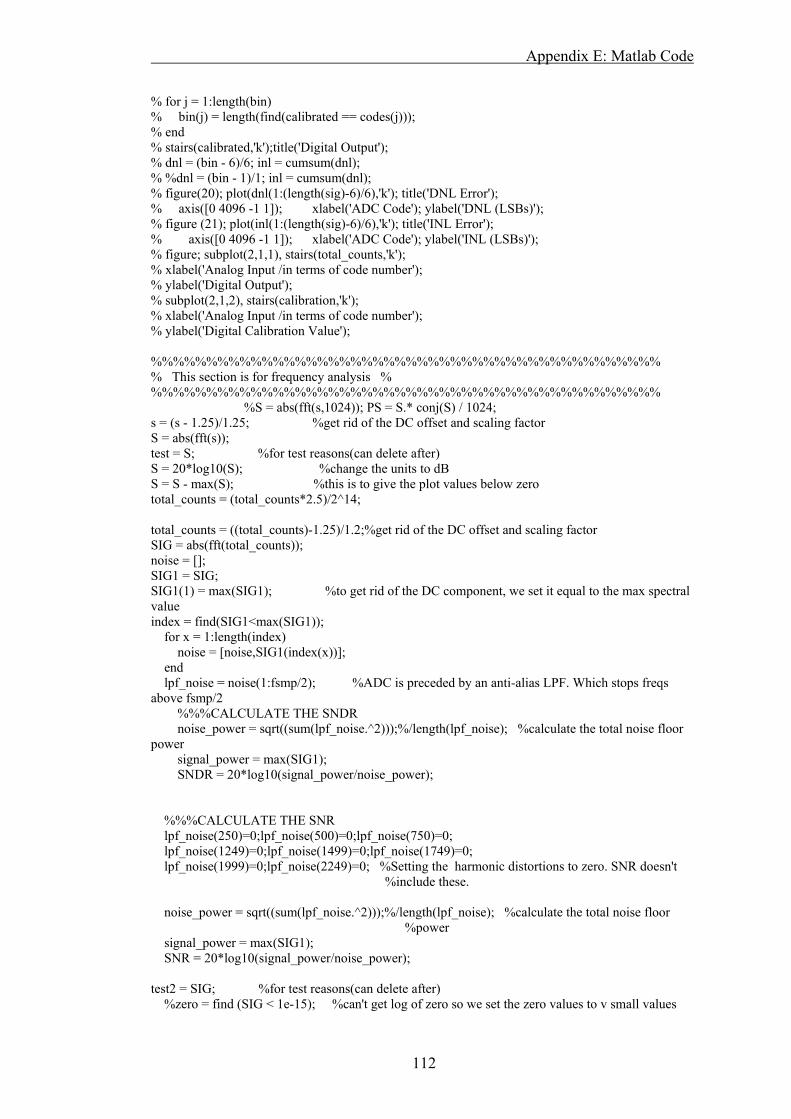
Appendix E: Matlab Code
% for j = 1:length(bin) % bin(j) = length(find(calibrated == codes(j))); % end % stairs(calibrated,'k');title('Digital Output'); % dnl = (bin - 6)/6; inl = cumsum(dnl); % %dnl = (bin - 1)/1; inl = cumsum(dnl); % figure(20); plot(dnl(1:(length(sig)-6)/6),'k'); title('DNL Error'); % axis([0 4096 -1 1]); xlabel('ADC Code'); ylabel('DNL (LSBs)'); % figure (21); plot(inl(1:(length(sig)-6)/6),'k'); title('INL Error'); % axis([0 4096 -1 1]); xlabel('ADC Code'); ylabel('INL (LSBs)'); % figure; subplot(2,1,1), stairs(total_counts,'k'); % xlabel('Analog Input /in terms of code number'); % ylabel('Digital Output'); % subplot(2,1,2), stairs(calibration,'k'); % xlabel('Analog Input /in terms of code number'); % ylabel('Digital Calibration Value'); %%%%%%%%%%%%%%%%%%%%%%%%%%%%%%%%%%%%%%%%%%%%%% % This section is for frequency analysis % %%%%%%%%%%%%%%%%%%%%%%%%%%%%%%%%%%%%%%%%%%%%%% %S = abs(fft(s,1024)); PS = S.* conj(S) / 1024; s = (s - 1.25)/1.25; %get rid of the DC offset and scaling factor S = abs(fft(s)); test = S; %for test reasons(can delete after) S = 20*log10(S); %change the units to dB S = S - max(S); %this is to give the plot values below zero total_counts = (total_counts*2.5)/2^14; total_counts = ((total_counts)-1.25)/1.2;%get rid of the DC offset and scaling factor SIG = abs(fft(total_counts)); noise = []; SIG1 = SIG; SIG1(1) = max(SIG1); %to get rid of the DC component, we set it equal to the max spectral value index = find(SIG1<max(SIG1)); for x = 1:length(index) noise = [noise,SIG1(index(x))]; end lpf_noise = noise(1:fsmp/2); %ADC is preceded by an anti-alias LPF. Which stops freqs above fsmp/2 %%%CALCULATE THE SNDR noise_power = sqrt((sum(lpf_noise.^2)));%/length(lpf_noise); %calculate the total noise floor power signal_power = max(SIG1); SNDR = 20*log10(signal_power/noise_power); %%%CALCULATE THE SNR lpf_noise(250)=0;lpf_noise(500)=0;lpf_noise(750)=0; lpf_noise(1249)=0;lpf_noise(1499)=0;lpf_noise(1749)=0; lpf_noise(1999)=0;lpf_noise(2249)=0; %Setting the harmonic distortions to zero. SNR doesn't %include these. noise_power = sqrt((sum(lpf_noise.^2)));%/length(lpf_noise); %calculate the total noise floor %power signal_power = max(SIG1); SNR = 20*log10(signal_power/noise_power); test2 = SIG; %for test reasons(can delete after) %zero = find (SIG < 1e-15); %can't get log of zero so we set the zero values to v small values
112

Appendix E: Matlab Code
%SIG(zero) = 1e-15; SIG = 20*log10(SIG); %changes the units to dB SIG = SIG - max(SIG); %normalise so that the fundamantal has a magnitude of 0 figure(9); plot(0:length(S)-1,S,'k'); title('FFT spectrum of input signal'); xlabel('frequency'); ylabel('dBFS'); figure(10); plot(0:(length(SIG)/2)-1,SIG(1:length(SIG)/2),'k'); title('FFT spectrum of time-interleaved ADC'); xlabel('frequency'); ylabel('dBFS'); grid; 12-bit time-interleaved pipeline ADC %this function m-file simulates a 12-bit four channel time-interleaved pipeline ADC format long; fsig = 5e6; %try 3e5 fsmp = 20e6; %try 1e6 ADC = 1; samp_freq=1e6; %desired sample frequency max_res = 6; %to achieve 1Msps (1e6) the clock freqency required is (2^6)1e6 clock_freq = (2^6)*samp_freq; %64MHz clk_period = 1/clock_freq; %15.625ns cap_time = clk_period/2; %should equal 7.8125ns Samp_Cap = 1e-12; %the sample capacitor on each channel T = 300; %temperatures in Kelvin k = 1.4*10^-23; %Boltzmanns Constant %%%%%%%%%%%%%%%%%%%%%%%%%%%%%%%%%%%%% % Generate sampled signal % % (Sample and Hold) % %%%%%%%%%%%%%%%%%%%%%%%%%%%%%%%%%%%%% j=0:0.0001:.9999; s = 1.25 + 1.25*sin(2*pi*fsig*j);% + 1.25*sin(2*pi*(fsig+fsig*.5)*j); i=(1/fsmp)*.5:1/fsmp:1; %delaying samples by one half period so that we're not %sampling at the zero crossings for j = 1:length(i) i(j) = i(j) + (rand*(2-1))*1e-12; %also addind clock jitter. pico seconds end sig = 1.25 + 1.2*sin(2*pi*fsig*i);% + 1.25*sin(2*pi*(fsig+fsig*.5)*i); %discrete time %sampled signal % plot(sig); % stem(i,sig,'r:'); hold on; stairs(i,sig,'r'); title('Sample and Hold signal');pause(1); %%%%%%%%%%%%%%%%%%%%%%%%%%%%%%%%%%%%% % Generate All-Code Test for % % INL and DNL calculations % %%%%%%%%%%%%%%%%%%%%%%%%%%%%%%%%%%%%% % ideal_step = 0.0006103515625; %0.000152587890625; % %sig = [0:ideal_step:2.5-ideal_step]; %all code (ramp) signal % %sig = [0:ideal_step:ideal_step*2000]; %this is a shortened ramp to run the pgm faster (512) % sig = [0:ideal_step/6:2.5-ideal_step/6]; % %sig = [0:ideal_step/4:ideal_step*6000]; % %sig = 4.08935546875e-3; op=zeros(1,length(sig)); binary = ['000000000000']; %binary will be a matrix of digital values add = 0; %tells us how many inputs read nothing, if fs/fsig isn't divisible by four while rem(length(sig),4) ~= 0 %zero pad sig, so that the other channels are zero instead of undefined
113

Appendix E: Matlab Code
sig = [sig,0]; add=add+1; end %out = zeros(1,length(sig)); %the output has the same num of elements as the sampled sig % [rows,columns]=size(binary); % while rows < length(sig) % binary = [binary;'000000000000']; % [rows,columns]=size(binary); % end out = zeros(0,0); %out is initially an empty matrix %b = zeros(0,0); %%%%%%%%%%%%%%%%%%%%%%%%%%%%%%%%%%%%%%%%%%%%%%%%% % Time Interleaved (parallel) conversion % %%%%%%%%%%%%%%%%%%%%%%%%%%%%%%%%%%%%%%%%%%%%%%%%% shuffle = 1; % shuffle determines the order in which the channels sample the i/p % should reduce gain and offset effects to noise %NEXT LINE adds the thermal noise to each sample value for i = 1:length(sig) sig(i) = sig(i) + sqrt(k*T/(Samp_Cap*3))*(rand*2-1); %add thermal noise due to S/H. end for i = 1:4:length(sig) %the four channels. Not offset and gain errors can be added here. switch shuffle case 1 nd1 = twelve_bit_pipeline_ADC2_5_with_4_stages((sig(i)*.9992 - 9e-5),cap_time); %channel 1 nd2 = twelve_bit_pipeline_ADC2_5_with_4_stages((sig(i+1)*.9999 + 3e-5),cap_time); %channel 2 nd3 = twelve_bit_pipeline_ADC2_5_with_4_stages((sig(i+2)*1.0004 - 1e-5),cap_time); %channel 3 nd4 = twelve_bit_pipeline_ADC2_5_with_4_stages((sig(i+3)*1.0002 + 2e-5),cap_time); %channel 4 out = [out,nd1,nd2,nd3,nd4]; shuffle = ceil(rand*5); case 2 nd1 = twelve_bit_pipeline_ADC2_5_with_4_stages((sig(i+2)*0.9992 - 9e-5),cap_time); nd2 = twelve_bit_pipeline_ADC2_5_with_4_stages((sig(i+3)*0.9999 + 3e-5),cap_time); nd3 = twelve_bit_pipeline_ADC2_5_with_4_stages((sig(i+1)*1.0004 - 1e-5),cap_time); nd4 = twelve_bit_pipeline_ADC2_5_with_4_stages((sig(i)*1.0002 + 2e-5),cap_time); out = [out,nd4,nd3,nd1,nd2]; shuffle = ceil(rand*5); case 3 nd1 = twelve_bit_pipeline_ADC2_5_with_4_stages((sig(i+1)*0.9992 - 9e-5),cap_time); nd2 = twelve_bit_pipeline_ADC2_5_with_4_stages((sig(i)*0.9999 + 3e-5),cap_time); nd3 = twelve_bit_pipeline_ADC2_5_with_4_stages((sig(i+3)*1.0004 - 1e-5),cap_time); nd4 = twelve_bit_pipeline_ADC2_5_with_4_stages((sig(i+2)*1.0002 + 2e-5),cap_time); out = [out,nd2,nd1,nd4,nd3]; shuffle = ceil(rand*5); case 4 nd1 = twelve_bit_pipeline_ADC2_5_with_4_stages((sig(i+3)*0.9992 - 9e-5),cap_time); nd2 = twelve_bit_pipeline_ADC2_5_with_4_stages((sig(i+2)*0.9999 + 3e-5),cap_time); nd3 = twelve_bit_pipeline_ADC2_5_with_4_stages((sig(i)*1.0004 - 1e-5),cap_time); nd4 = twelve_bit_pipeline_ADC2_5_with_4_stages((sig(i+1)*1.0002 + 2e-5),cap_time);
114

Appendix E: Matlab Code
out = [out,nd3,nd4,nd2,nd1]; shuffle = ceil(rand*5); case 5 nd1 = twelve_bit_pipeline_ADC2_5_with_4_stages((sig(i+3)*0.9992 - 9e-5),cap_time); nd2 = twelve_bit_pipeline_ADC2_5_with_4_stages((sig(i+2)*0.9999 + 3e-5),cap_time); nd3 = twelve_bit_pipeline_ADC2_5_with_4_stages((sig(i+1)*1.0004 - 1e-5),cap_time); nd4 = twelve_bit_pipeline_ADC2_5_with_4_stages((sig(i)*1.0002 + 2e-5),cap_time); out = [out,nd4,nd3,nd2,nd1]; shuffle = ceil(rand*5); end end total_counts = out; %%%%%%%%%%%%%%%%%%%%%%%%%%%%%%%%%%%%%%%%%%%%%%%%% % This section performs calibration and linearity analysis % %%%%%%%%%%%%%%%%%%%%%%%%%%%%%%%%%%%%%%%%%%%%%%%%% % calibrated = total_counts;%calibrate(total_counts);% + amend.calibration; % % bin = zeros(1,2^12); codes = 0:2^12-1; % for j = 1:length(bin) % bin(j) = length(find(calibrated == codes(j))); % end % stairs(calibrated,'k');title('Digital Output'); % dnl = (bin - 6)/6; inl = cumsum(dnl); % %dnl = (bin - 1)/1; inl = cumsum(dnl); % figure(20); plot(dnl(1:(length(sig)-6)/6),'k'); title('DNL Error'); % axis([0 4096 -1 1]); xlabel('ADC Code'); ylabel('DNL (LSBs)'); % figure (21); plot(inl(1:(length(sig)-6)/6),'k'); title('INL Error'); % axis([0 4096 -1 1]); xlabel('ADC Code'); ylabel('INL (LSBs)'); % figure; subplot(2,1,1), stairs(total_counts,'k'); % xlabel('Analog Input /in terms of code number'); % ylabel('Digital Output'); % subplot(2,1,2), stairs(calibration,'k'); % xlabel('Analog Input /in terms of code number'); % ylabel('Digital Calibration Value'); %%%%%%%%%%%%%%%%%%%%%%%%%%%%%%%%%%%%%%%%%%%%%% % This section is for frequency analysis % %%%%%%%%%%%%%%%%%%%%%%%%%%%%%%%%%%%%%%%%%%%%%% %S = abs(fft(s,1024)); PS = S.* conj(S) / 1024; s = (s - 1.25)/1.25; %get rid of the DC offset and scaling factor S = abs(fft(s)); test = S; %for test reasons(can delete after) S = 20*log10(S); %change the units to dB S = S - max(S); %this is to give the plot values below zero total_counts = (total_counts*2.5)/2^14; total_counts = ((total_counts)-1.25)/1.2;%get rid of the DC offset and scaling factor SIG = abs(fft(total_counts)); noise = []; SIG1 = SIG; SIG1(1) = max(SIG1); %to get rid of the DC component, we set it equal to the max spectral value index = find(SIG1<max(SIG1)); for x = 1:length(index) noise = [noise,SIG1(index(x))]; end
115

Appendix E: Matlab Code
116
lpf_noise = noise(1:fsmp/2); %ADC is preceded by an anti-alias LPF. Which stops freqs above fsmp/2 %%%CALCULATE THE SNDR noise_power = sqrt((sum(lpf_noise.^2)));%/length(lpf_noise); %calculate the total noise floor %power signal_power = max(SIG1); SNDR = 20*log10(signal_power/noise_power); %%%CALCULATE THE SNR lpf_noise(250)=0;lpf_noise(500)=0;lpf_noise(750)=0; lpf_noise(1249)=0;lpf_noise(1499)=0;lpf_noise(1749)=0; lpf_noise(1999)=0;lpf_noise(2249)=0; %Setting the spurious distortions to zero. SNR doesn't %include these. noise_power = sqrt((sum(lpf_noise.^2)));%/length(lpf_noise); %calculate the total noise floor %power signal_power = max(SIG1); SNR = 20*log10(signal_power/noise_power); test2 = SIG; %for test reasons(can delete after) SIG = 20*log10(SIG); %changes the units to dB SIG = SIG - max(SIG); %normalise so that the fundamantal has a magnitude of 0 figure(9); plot(0:length(S)-1,S,'k'); title('FFT spectrum of input signal'); xlabel('frequency'); ylabel('dBFS'); %figure(10); stem(f2,PSIG); %figure(10); plot(0:length(SIG)-1,SIG,'k'); title('FFT spectrum of 14-bitADC'); xlabel('frequency'); ylabel('dBFS'); figure(10); plot(0:(length(SIG)/2)-1,SIG(1:length(SIG)/2),'k'); title('FFT spectrum of time-interleaved ADC'); xlabel('frequency'); ylabel('dBFS'); grid;

Appendix F
Recurrence Equations
Table E.1 shows the mathematically derived recurrence equations to achieve the
maximum period for 2 to 8 bit LFSRs.
M Recurrence Equation
2 xn-1 ⊕ xn-2
3 xn-1 ⊕ xn-3
4 xn-1 ⊕ xn-4
5 xn-2 ⊕ xn-5
6 xn-1 ⊕ xn-6
7 xn-1 ⊕ xn-7
8 xn-2 ⊕ xn-3 ⊕ xn-4 ⊕ xn-8
Table E.1 Sample Recurrence Equations [43] (i.e. Design Techniques of FPGA based Random Number Generator, Pong P. Chu
and Robert E. Jones)

Appendix G
Mentor Simulation Analysis Load_vars.m %Script m-file to load the output variables of the mentor siimulation %into the matlab workspace time = load('nigel_node_time')'; display('Time Vector Loaded'); Vsig = load('nigel_V_node_VSIG')'; display('Input signal loaded'); hold1 = load('nigel_V_node_VHOLD1')'; hold2 = load('nigel_V_node_VHOLD2')'; hold3 = load('nigel_V_node_VHOLD3')'; hold4 = load('nigel_V_node_VHOLD4')'; hold5 = load('nigel_V_node_VHOLD5')'; hold6 = load('nigel_V_node_VHOLD6')'; hold7 = load('nigel_V_node_VHOLD7')'; hold8 = load('nigel_V_node_VHOLD8')'; display('Sample and Hold Signals loaded'); ramp1 = load('nigel_V_node_V_RAMP')'; ramp2 = load('nigel_V_node_V_RAMP2')'; display('CS ramps loaded'); trig1 = load('nigel_V_node_TRIGGER1')'; trig2 = load('nigel_V_node_TRIGGER2')'; trig3 = load('nigel_V_node_TRIGGER3')'; trig4 = load('nigel_V_node_TRIGGER4')'; trig5 = load('nigel_V_node_TRIGGER5')'; trig6 = load('nigel_V_node_TRIGGER6')'; trig7 = load('nigel_V_node_TRIGGER7')'; trig8 = load('nigel_V_node_TRIGGER8')'; display('Comparator Outputs loaded'); VS1 = load('nigel_V_node_S1')'; VS2 = load('nigel_V_node_S2')'; VS3 = load('nigel_V_node_S3')'; VS4 = load('nigel_V_node_S4')'; VS5 = load('nigel_V_node_S5')'; VS6 = load('nigel_V_node_S6')'; VS7 = load('nigel_V_node_S7')'; VS8 = load('nigel_V_node_S8')'; display('Sampling instances loaded');

Appendix G: Mentor Simulation Analysis
trigger_instance.m %script m-file to determine the time instance of each ramp triggering %i.e. takes trig1 - trig8 and determines the element number when the %the comparator triggers %This part determines when the trigger volatge is on index1 = find(trig1 >= 2.8); index2 = find(trig2 >= 2.8); index3 = find(trig3 >= 2.8); index4 = find(trig4 >= 2.8); %index1 = index2; index4 = index3; index5 = find(trig5 >= 2.8); index6 = find(trig6 >= 2.8); index7 = find(trig7 >= 2.8); index8 = find(trig8 >= 2.8); %declare some variables indx1 = zeros(1,length(index1)); indx2 = zeros(1,length(index2)); indx3 = zeros(1,length(index3)); indx4 = zeros(1,length(index4)); indx5 = zeros(1,length(index5)); indx6 = zeros(1,length(index6)); indx7 = zeros(1,length(index7)); indx8 = zeros(1,length(index8)); %We only want the trigger instance so we must remove the index %numbers corresponding to when the trigger is continually on indx1(1) = index1(1); for i=2:length(index1) if (index1(i)-index1(i-1) > 128) %disp('here'); indx1(i) = index1(i); end end indx2(1) = index2(1); for i=2:length(index2) if index2(i)-index2(i-1) > 128 indx2(i) = index2(i); end end indx3(1) = index3(1); for i=2:length(index3) if index3(i)-index3(i-1) > 128 indx3(i) = index3(i); end end indx4(1) = index4(1); for i=2:length(index4) if index4(i)-index4(i-1) > 128 indx4(i) = index4(i); end end indx5(1) = index5(1); for i=2:length(index5) if index5(i)-index5(i-1) > 128 indx5(i) = index5(i);
119

Appendix G: Mentor Simulation Analysis
end end indx6(1) = index6(1); for i=2:length(index6) if index6(i)-index6(i-1) > 128 indx6(i) = index6(i); end end indx7(1) = index7(1); for i=2:length(index7) if index7(i)-index7(i-1) > 128 indx7(i) = index7(i); end end indx8(1) = index8(1); for i=2:length(index8) if index8(i)-index8(i-1) > 128 indx8(i) = index8(i); end end trigger1 = find(indx1 > 0); time1 = (indx1(trigger1)); %this produces the element numbers of the time vector where COMPARATOR1 triggered trigger2 = find(indx2 > 0); time2 = (indx2(trigger2)); %this produces the element numbers of the time vector where COMPARATOR2 triggered trigger3 = find(indx3 > 0); time3 = (indx3(trigger3)); trigger4 = find(indx4 > 0); time4 = (indx4(trigger4)); trigger5 = find(indx5 > 0); time5 = (indx5(trigger5)); trigger6 = find(indx6 > 0); time6 = (indx6(trigger6)); trigger7 = find(indx7 > 0); time7 = (indx7(trigger7)); trigger8 = find(indx8 > 0); time8 = (indx8(trigger8)); %Clear the variables that are no longer needed clear index1 index2 index3 index4 index5 index6 index7 index8; clear indx1 indx2 indx3 indx4 indx5 indx6 indx6 indx7 indx8; clear trigger1 trigger2 trigger3 trigger4 trigger5 trigger6 trigger7 trigger8; %subplot(4,1,1),plot(trig5); subplot(4,1,2),plot(trig6,'r'); %subplot(4,1,3),plot(trig7,'g'); subplot(4,1,4),plot(trig8,'y');
120

Appendix G: Mentor Simulation Analysis
% %%%%%%%%%%%%%%%%%%%%%%%%%%%%%%%%%%%%%%% % %%NON RANDOMIZATION % %Combine the trigger times for each bank of comparators to create two % %trigger time vectors % time_SH1 = []; time_SH2 = []; % for i = 1:length(time1) %%%TAKE THE -1 AWAY LATER % time_SH1 = [time_SH1,time1(i),time2(i),time3(i),time4(i)]; %the first bank of comparators % end % % for i = 1:length(time5) % time_SH2 = [time_SH2,time5(i),time6(i),time7(i),time8(i)]; %the second bank of comparators % end %%%%%%%%%%%%%%%%%%%%%%%%%%%%%%%%%%%%%%%% %%RANDOMIZATION %Combine the trigger times for each bank of comparators to create two %trigger time vectors sample_sequence; %runs the script m-file to calculate the sampling equence used. creates sequence1 and sequence2 time_SH1 = []; time_SH2 = []; for i = 1:length(time1) %the first bank of comparators switch sequence1(i) case 1 %S1,S2,S3,S4 time_SH1 = [time_SH1,time1(i),time2(i),time3(i),time4(i)]; case 2 %S1,S2,S4,S3 time_SH1 = [time_SH1,time1(i),time2(i),time4(i),time3(i)]; case 3 %S1,S3,S2,S4 time_SH1 = [time_SH1,time1(i),time3(i),time2(i),time4(i)]; case 4 %S1,S3,S4,S2 time_SH1 = [time_SH1,time1(i),time3(i),time4(i),time2(i)]; case 5 %S1,S4,S2,S3 time_SH1 = [time_SH1,time1(i),time4(i),time2(i),time3(i)]; case 6 %S1,S4,S3,S2 time_SH1 = [time_SH1,time1(i),time4(i),time3(i),time2(i)]; case 7 %S2,S1,S3,S4 time_SH1 = [time_SH1,time2(i),time1(i),time3(i),time4(i)]; case 8 %S2,S1,S4,S3 time_SH1 = [time_SH1,time2(i),time1(i),time4(i),time3(i)]; case 9 %S2,S3,S1,S4 time_SH1 = [time_SH1,time2(i),time3(i),time1(i),time4(i)]; case 10 %S2,S3,S4,S1 time_SH1 = [time_SH1,time2(i),time3(i),time4(i),time1(i)]; case 11 %S2,S4,S1,S3 time_SH1 = [time_SH1,time2(i),time4(i),time1(i),time3(i)]; case 12 %S2,S4,S3,S1 time_SH1 = [time_SH1,time2(i),time4(i),time3(i),time1(i)]; case 13 %S3,S1,S2,S4 time_SH1 = [time_SH1,time3(i),time1(i),time2(i),time4(i)]; case 14 %S3,S1,S4,S2 time_SH1 = [time_SH1,time3(i),time1(i),time4(i),time2(i)]; case 15 %S3,S2,S1,S4 time_SH1 = [time_SH1,time3(i),time2(i),time1(i),time4(i)]; case 16 %S3,S2,S4,S1 time_SH1 = [time_SH1,time3(i),time2(i),time4(i),time1(i)]; case 17 %S3,S4,S1,S2 time_SH1 = [time_SH1,time3(i),time4(i),time1(i),time2(i)]; case 18 %S3,S4,S2,S1 time_SH1 = [time_SH1,time3(i),time4(i),time2(i),time1(i)]; case 19 %S4,S1,S2,S3
121

Appendix G: Mentor Simulation Analysis
time_SH1 = [time_SH1,time4(i),time1(i),time2(i),time3(i)]; case 20 %S4,S1,S3,S2 time_SH1 = [time_SH1,time4(i),time1(i),time3(i),time2(i)]; case 21 %S4,S2,S1,S3 time_SH1 = [time_SH1,time4(i),time2(i),time1(i),time3(i)]; case 22 %S4,S2,S3,S1 time_SH1 = [time_SH1,time4(i),time2(i),time3(i),time1(i)]; case 23 %S4,S3,S1,S2 time_SH1 = [time_SH1,time4(i),time3(i),time1(i),time2(i)]; case 24 %S4,S3,S2,S1 time_SH1 = [time_SH1,time4(i),time3(i),time2(i),time1(i)]; case 25 %S1,S2,S3,S4 time_SH1 = [time_SH1,time1(i),time2(i),time3(i),time4(i)]; case 26 %S1,S3,S2,S4 time_SH1 = [time_SH1,time1(i),time3(i),time2(i),time4(i)]; case 27 %S1,S4,S3,S2 time_SH1 = [time_SH1,time1(i),time4(i),time3(i),time2(i)]; case 28 %S2,S4,S1,S3 time_SH1 = [time_SH1,time2(i),time4(i),time1(i),time3(i)]; case 29 %S3,S2,S1,S4 time_SH1 = [time_SH1,time3(i),time2(i),time1(i),time4(i)]; case 30 %S3,S4,S2,S1 time_SH1 = [time_SH1,time3(i),time4(i),time2(i),time1(i)]; case 31 %S4,S1,S3,S2 time_SH1 = [time_SH1,time4(i),time1(i),time3(i),time2(i)]; case 32 %S4,S2,S3,S1 time_SH1 = [time_SH1,time4(i),time2(i),time3(i),time1(i)]; end end for j = 1:length(time5) %the second bank of comparators switch sequence2(j) case 1 %S5,S6,S7,S8 time_SH2 = [time_SH2,time5(j),time6(j),time7(j),time8(j)]; case 2 %S5,S6,S8,S7 time_SH2 = [time_SH2,time5(j),time6(j),time8(j),time7(j)]; case 3 %S5,S7,S6,S8 time_SH2 = [time_SH2,time5(j),time7(j),time6(j),time8(j)]; case 4 %S5,S7,S8,S6 time_SH2 = [time_SH2,time5(j),time7(j),time8(j),time6(j)]; case 5 %S5,S8,S6,S7 time_SH2 = [time_SH2,time5(j),time8(j),time6(j),time7(j)]; case 6 %S5,S8,S7,S6 time_SH2 = [time_SH2,time5(j),time8(j),time7(j),time6(j)]; case 7 %S6,S5,S7,S8 time_SH2 = [time_SH2,time6(j),time5(j),time7(j),time8(j)]; case 8 %S6,S5,S8,S7 time_SH2 = [time_SH2,time6(j),time5(j),time8(j),time7(j)]; case 9 %S6,S7,S5,S8 time_SH2 = [time_SH2,time6(j),time7(j),time5(j),time8(j)]; case 10 %S6,S7,S8,S5 time_SH2 = [time_SH2,time6(j),time7(j),time8(j),time5(j)]; case 11 %S6,S8,S5,S7 time_SH2 = [time_SH2,time6(j),time8(j),time5(j),time7(j)]; case 12 %S6,S8,S7,S5 time_SH2 = [time_SH2,time6(j),time8(j),time7(j),time5(j)]; case 13 %S7,S5,S6,S8 time_SH2 = [time_SH2,time7(j),time5(j),time6(j),time8(j)]; case 14 %S7,S5,S8,S6 time_SH2 = [time_SH2,time7(j),time5(j),time8(j),time6(j)];
122

Appendix G: Mentor Simulation Analysis
case 15 %S7,S6,S5,S8 time_SH2 = [time_SH2,time7(j),time6(j),time5(j),time8(j)]; case 16 %S7,S6,S8,S5 time_SH2 = [time_SH2,time7(j),time6(j),time8(j),time5(j)]; case 17 %S7,S8,S5,S6 time_SH2 = [time_SH2,time7(j),time8(j),time5(j),time6(j)]; case 18 %S7,S8,S6,S5 time_SH2 = [time_SH2,time7(j),time8(j),time6(j),time5(j)]; case 19 %S8,S5,S6,S7 time_SH2 = [time_SH2,time8(j),time5(j),time6(j),time7(j)]; case 20 %S8,S5,S7,S6 time_SH2 = [time_SH2,time8(j),time5(j),time7(j),time6(j)]; case 21 %S8,S6,S5,S7 time_SH2 = [time_SH2,time8(j),time6(j),time5(j),time7(j)]; case 22 %S8,S6,S7,S5 time_SH2 = [time_SH2,time8(j),time6(j),time7(j),time5(j)]; case 23 %S8,S7,S5,S6 time_SH2 = [time_SH2,time8(j),time7(j),time5(j),time6(j)]; case 24 %S8,S7,S6,S5 time_SH2 = [time_SH2,time8(j),time7(j),time6(j),time5(j)]; case 25 %S5,S6,S7,S8 time_SH2 = [time_SH2,time5(j),time6(j),time7(j),time8(j)]; case 26 %S5,S7,S6,S8 time_SH2 = [time_SH2,time5(j),time7(j),time6(j),time8(j)]; case 27 %S5,S8,S7,S6 time_SH2 = [time_SH2,time5(j),time8(j),time7(j),time6(j)]; case 28 %S6,S8,S5,S7 time_SH2 = [time_SH2,time6(j),time8(j),time5(j),time7(j)]; case 29 %S7,S6,S5,S8 time_SH2 = [time_SH2,time7(j),time6(j),time5(j),time8(j)]; case 30 %S7,S8,S6,S5 time_SH2 = [time_SH2,time7(j),time8(j),time6(j),time5(j)]; case 31 %S8,S5,S7,S6 time_SH2 = [time_SH2,time8(j),time5(j),time7(j),time6(j)]; case 32 %S8,S6,S7,S5 time_SH2 = [time_SH2,time8(j),time6(j),time7(j),time5(j)]; end end %%%%%%%%%%%%%%%%%%%%%%%%%%%%%%%%%%%
123

Appendix G: Mentor Simulation Analysis
sample_sequence.m %%% script m-file to determine the sampling sequence on1 = find(VS1 >= 2.8); on2 = find(VS2 >= 2.8); on3 = find(VS3 >= 2.8); on4 = find(VS4 >= 2.8); on5 = find(VS5 >= 2.8); on6 = find(VS6 >= 2.8); on7 = find(VS7 >= 2.8); on8 = find(VS8 >= 2.8); edge1 = zeros(1,length(on1)); edge2 = zeros(1,length(on2)); edge3 = zeros(1,length(on3)); edge4 = zeros(1,length(on4)); edge5 = zeros(1,length(on5)); edge6 = zeros(1,length(on6)); edge7 = zeros(1,length(on7)); edge8 = zeros(1,length(on8)); %edge1(1) = on1(1); for i=2:length(on1) if (on1(i)-on1(i-1) > 128) %disp('here'); edge1(i-1) = on1(i); %-1 because 1st bank of switches are 1 to begin with end end %edge2(1) = on2(1); for i=2:length(on2) if (on2(i)-on2(i-1) > 128) %disp('here'); edge2(i-1) = on2(i); end end %edge3(1) = on3(1); for i=2:length(on3) if (on3(i)-on3(i-1) > 128) %disp('here'); edge3(i-1) = on3(i); end end %edge4(1) = on4(1); for i=2:length(on4) if (on4(i)-on4(i-1) > 128) %disp('here'); edge4(i-1) = on4(i); end end edge5(1) = on5(1); for i=2:length(on5) if (on5(i)-on5(i-1) > 128) %disp('here'); edge5(i) = on5(i); end end
124

Appendix G: Mentor Simulation Analysis
edge6(1) = on6(1); for i=2:length(on6) if (on6(i)-on6(i-1) > 128) %disp('here'); edge6(i) = on6(i); end end edge7(1) = on7(1); for i=2:length(on7) if (on7(i)-on7(i-1) > 128) %disp('here'); edge7(i) = on7(i); end end edge8(1) = on8(1); for i=2:length(on8) if (on8(i)-on8(i-1) > 128) %disp('here'); edge8(i) = on8(i); end end trigger_edge1 = find(edge1 > 0); t1 = edge1(trigger_edge1); trigger_edge2 = find(edge2 > 0); t2 = edge2(trigger_edge2); trigger_edge3 = find(edge3 > 0); t3 = edge3(trigger_edge3); trigger_edge4 = find(edge4 > 0); t4 = edge4(trigger_edge4); trigger_edge5 = find(edge5 > 0); t5 = edge5(trigger_edge5); trigger_edge6 = find(edge6 > 0); t6 = edge6(trigger_edge6); trigger_edge7 = find(edge7 > 0); t7 = edge7(trigger_edge7); trigger_edge8 = find(edge8 > 0); t8 = edge8(trigger_edge8); clear on1 on2 on3 on4 on5 on6 on7 on8; clear edge1 edge2 edge3 edge4 edge5 edge6 edge6 edge7 edge8; subplot(8,1,1), plot(VS1); ylabel('S1'); subplot(8,1,2), plot(VS2); ylabel('S2'); subplot(8,1,3), plot(VS3); ylabel('S3'); subplot(8,1,4), plot(VS4); ylabel('S4'); subplot(8,1,5), plot(VS5); ylabel('S5'); subplot(8,1,6), plot(VS6); ylabel('S6'); subplot(8,1,7), plot(VS7); ylabel('S7'); subplot(8,1,8), plot(VS8); ylabel('S8'); sequence1 = zeros(1,length(t1)); sequence2 = zeros(1,length(t5)); for i = 1:length(t1) a = [t1(i),t2(i),t3(i),t4(i)];
125

Appendix G: Mentor Simulation Analysis
a = sort(a); if (a(1)==t1(i)&& a(2)==t2(i)&& a(3)==t3(i)&& a(4)==t4(i)) sequence1(i) = 1; elseif(a(1)==t1(i)&& a(2)==t2(i)&& a(3)==t4(i)&& a(4)==t3(i)) sequence1(i) = 2; elseif (a(1)==t1(i)&& a(2)==t3(i)&& a(3)==t2(i)&& a(4)==t4(i)) sequence1(i) = 3; elseif (a(1)==t1(i)&& a(2)==t3(i)&& a(3)==t4(i)&& a(4)==t2(i)) sequence1(i) = 4; elseif (a(1)==t1(i)&& a(2)==t4(i)&& a(3)==t2(i)&& a(4)==t3(i)) sequence1(i) = 5; elseif (a(1)==t1(i)&& a(2)==t4(i)&& a(3)==t3(i)&& a(4)==t2(i)) sequence1(i) = 6; elseif (a(1)==t2(i)&& a(2)==t1(i)&& a(3)==t3(i)&& a(4)==t4(i)) sequence1(i) = 7; elseif (a(1)==t2(i)&& a(2)==t1(i)&& a(3)==t4(i)&& a(4)==t3(i)) sequence1(i) = 8; elseif (a(1)==t2(i)&& a(2)==t3(i)&& a(3)==t1(i)&& a(4)==t4(i)) sequence1(i) = 9; elseif (a(1)==t2(i)&& a(2)==t3(i)&& a(3)==t4(i)&& a(4)==t1(i)) sequence1(i) = 10; elseif (a(1)==t2(i)&& a(2)==t4(i)&& a(3)==t1(i)&& a(4)==t3(i)) sequence1(i) = 11; elseif (a(1)==t2(i)&& a(2)==t4(i)&& a(3)==t3(i)&& a(4)==t1(i)) sequence1(i) = 12; elseif (a(1)==t3(i)&& a(2)==t1(i)&& a(3)==t2(i)&& a(4)==t4(i)) sequence1(i) = 13; elseif (a(1)==t3(i)&& a(2)==t1(i)&& a(3)==t4(i)&& a(4)==t2(i)) sequence1(i) = 14; elseif (a(1)==t3(i)&& a(2)==t2(i)&& a(3)==t1(i)&& a(4)==t4(i)) sequence1(i) = 15; elseif (a(1)==t3(i)&& a(2)==t2(i)&& a(3)==t4(i)&& a(4)==t1(i)) sequence1(i) = 16; elseif (a(1)==t3(i)&& a(2)==t4(i)&& a(3)==t1(i)&& a(4)==t1(i)) sequence1(i) = 17; elseif (a(1)==t3(i)&& a(2)==t4(i)&& a(3)==t2(i)&& a(4)==t1(i)) sequence1(i) = 18; elseif (a(1)==t4(i)&& a(2)==t1(i)&& a(3)==t2(i)&& a(4)==t3(i)) sequence1(i) = 19; elseif (a(1)==t4(i)&& a(2)==t1(i)&& a(3)==t3(i)&& a(4)==t2(i)) sequence1(i) = 20; elseif (a(1)==t4(i)&& a(2)==t2(i)&& a(3)==t1(i)&& a(4)==t3(i)) sequence1(i) = 21; elseif (a(1)==t4(i)&& a(2)==t2(i)&& a(3)==t3(i)&& a(4)==t1(i)) sequence1(i) = 22; elseif (a(1)==t4(i)&& a(2)==t3(i)&& a(3)==t1(i)&& a(4)==t2(i)) sequence1(i) = 23; elseif (a(1)==t4(i)&& a(2)==t3(i)&& a(3)==t2(i)&& a(4)==t1(i)) sequence1(i) = 24; elseif (a(1)==t1(i)&& a(2)==t2(i)&& a(3)==t3(i)&& a(4)==t4(i)) sequence1(i) = 25; elseif (a(1)==t1(i)&& a(2)==t3(i)&& a(3)==t2(i)&& a(4)==t4(i)) sequence1(i) = 26; elseif (a(1)==t1(i)&& a(2)==t4(i)&& a(3)==t3(i)&& a(4)==t2(i)) sequence1(i) = 27; elseif (a(1)==t2(i)&& a(2)==t4(i)&& a(3)==t1(i)&& a(4)==t3(i)) sequence1(i) = 28; elseif (a(1)==t3(i)&& a(2)==t2(i)&& a(3)==t1(i)&& a(4)==t4(i)) sequence1(i) = 28;
126

Appendix G: Mentor Simulation Analysis
elseif (a(1)==t3(i)&& a(2)==t4(i)&& a(3)==t2(i)&& a(4)==t1(i)) sequence1(i) = 30; elseif (a(1)==t4(i)&& a(2)==t1(i)&& a(3)==t3(i)&& a(4)==t2(i)) sequence1(i) = 31; else %if(a(1)==t4(i)&& a(2)==t2(i)&& a(3)==t3(i)&& a(4)==t1(i)) sequence1(i) = 32; end end for j = 1:length(t8) a = [t5(j),t6(j),t7(j),t8(j)]; a = sort(a); if (a(1)==t5(j)&& a(2)==t6(j)&& a(3)==t7(j)&& a(4)==t8(j)) sequence2(j) = 1; elseif(a(1)==t5(j)&& a(2)==t6(j)&& a(3)==t8(j)&& a(4)==t7(j)) sequence2(j) = 2; elseif (a(1)==t5(j)&& a(2)==t7(j)&& a(3)==t6(j)&& a(4)==t8(j)) sequence2(j) = 3; elseif (a(1)==t5(j)&& a(2)==t7(j)&& a(3)==t8(j)&& a(4)==t6(j)) sequence2(j) = 4; elseif (a(1)==t5(j)&& a(2)==t8(j)&& a(3)==t6(j)&& a(4)==t7(j)) sequence2(j) = 5; elseif (a(1)==t5(j)&& a(2)==t8(j)&& a(3)==t7(j)&& a(4)==t6(j)) sequence2(j) = 6; elseif (a(1)==t6(j)&& a(2)==t5(j)&& a(3)==t7(j)&& a(4)==t8(j)) sequence2(j) = 7; elseif (a(1)==t6(j)&& a(2)==t5(j)&& a(3)==t8(j)&& a(4)==t7(j)) sequence2(j) = 8; elseif (a(1)==t6(j)&& a(2)==t7(j)&& a(3)==t5(j)&& a(4)==t8(j)) sequence2(j) = 9; elseif (a(1)==t6(j)&& a(2)==t7(j)&& a(3)==t8(j)&& a(4)==t5(j)) sequence2(j) = 10; elseif (a(1)==t6(j)&& a(2)==t8(j)&& a(3)==t5(j)&& a(4)==t7(j)) sequence2(j) = 11; elseif (a(1)==t6(j)&& a(2)==t8(j)&& a(3)==t7(j)&& a(4)==t5(j)) sequence2(j) = 12; elseif (a(1)==t7(j)&& a(2)==t5(j)&& a(3)==t6(j)&& a(4)==t8(j)) sequence2(j) = 13; elseif (a(1)==t7(j)&& a(2)==t5(j)&& a(3)==t8(j)&& a(4)==t6(j)) sequence2(j) = 14; elseif (a(1)==t7(j)&& a(2)==t6(j)&& a(3)==t5(j)&& a(4)==t8(j)) sequence2(j) = 15; elseif (a(1)==t7(j)&& a(2)==t6(j)&& a(3)==t8(j)&& a(4)==t5(j)) sequence2(j) = 16; elseif (a(1)==t7(j)&& a(2)==t8(j)&& a(3)==t5(j)&& a(4)==t5(j)) sequence2(j) = 17; elseif (a(1)==t7(j)&& a(2)==t8(j)&& a(3)==t6(j)&& a(4)==t5(j)) sequence2(j) = 18; elseif (a(1)==t8(j)&& a(2)==t5(j)&& a(3)==t6(j)&& a(4)==t7(j)) sequence2(j) = 19; elseif (a(1)==t8(j)&& a(2)==t5(j)&& a(3)==t7(j)&& a(4)==t6(j)) sequence2(j) = 20; elseif (a(1)==t8(j)&& a(2)==t6(j)&& a(3)==t5(j)&& a(4)==t7(j)) sequence2(j) = 21; elseif (a(1)==t8(j)&& a(2)==t6(j)&& a(3)==t7(j)&& a(4)==t5(j)) sequence2(j) = 22; elseif (a(1)==t8(j)&& a(2)==t7(j)&& a(3)==t5(j)&& a(4)==t6(j)) sequence2(j) = 23; elseif (a(1)==t8(j)&& a(2)==t7(j)&& a(3)==t6(j)&& a(4)==t5(j))
127

Appendix G: Mentor Simulation Analysis
sequence2(j) = 24; elseif (a(1)==t5(j)&& a(2)==t6(j)&& a(3)==t7(j)&& a(4)==t8(j)) sequence2(j) = 25; elseif (a(1)==t5(j)&& a(2)==t7(j)&& a(3)==t6(j)&& a(4)==t8(j)) sequence2(j) = 26; elseif (a(1)==t5(j)&& a(2)==t8(j)&& a(3)==t7(j)&& a(4)==t6(j)) sequence2(j) = 27; elseif (a(1)==t6(j)&& a(2)==t8(j)&& a(3)==t5(j)&& a(4)==t7(j)) sequence2(j) = 28; elseif (a(1)==t7(j)&& a(2)==t6(j)&& a(3)==t5(j)&& a(4)==t8(j)) sequence2(j) = 28; elseif (a(1)==t7(j)&& a(2)==t8(j)&& a(3)==t6(j)&& a(4)==t5(j)) sequence2(j) = 30; elseif (a(1)==t8(j)&& a(2)==t5(j)&& a(3)==t7(j)&& a(4)==t6(j)) sequence2(j) = 31; else %if(a(1)==t8(j)&& a(2)==t6(j)&& a(3)==t7(j)&& a(4)==t5(j)) sequence2(j) = 32; end end
128

Appendix G: Mentor Simulation Analysis
129
bin_out.m %m-file to interpret the proper count value i.e. 0-255 from the %triggering instances for non-randomisation sampling %NOTE: time is the overall time vector count = 1:264; %i.e. 256 + 8 for calibration clk_period = 1/66e6; %period of our ramp clock N = max(time)/clk_period; %the amount of clock periods in the total amount of time %Ramp_count = N/length(count); %the amount of ramps that have been used t = length(time)/N; %NB: divides the time vector into ramp clock periods count1 = time_SH1/t; %ramp1 is delayed by 3 SH periods. So, start at X - 256*3 count2 = time_SH2/t; %ramp2 is delayed by 2 SH periods. So, start at X - 256*2 %Need to take away the calibration count from the overall counts i.e. %6+2+6+2 = 16 for each clock period. Starting at 32+6 = 38. x = 38; y = 46; for i = 1:4:length(count2) count2(i:i+3) = floor(count2(i:i+3)-x); x = x+16; end %count2 for i = 1:4:length(count1) count1(i:i+3) = floor(count1(i:i+3)-y); y = y+16; end %The two count vectors need to be combined to form one count vector output_count = []; x = 2; %ramp2 is delayed by 2 SH periods. So, start at X - 256*2 y = 3; %ramp1 is delayed by 3 SH periods. So, start at X - 256*3 for i = 1:4:length(count2) count2(i:i+3) = count2(i:i+3)-256*x; x = x + 2; end for i = 1:4:length(count1) count1(i:i+3) = count1(i:i+3)-256*y; y = y + 2; end % output_count = [count2(1:4),count1(1:4),count2(5:8),count1(5:8),count2(9:12)]; for x = 1:4:length(count2)-4 output_count = [output_count,count2(x:x+3),count1(x:x+3)]; end %now add the last bit to output_count output_count = [output_count,count2(length(count2)-3:length(count2)),count1(length(count1)-3:length(count1))]; freq = 1:66e6/length(output_count):66e6-1; plot(freq,abs(fft(output_count-128))); % plot(freq,abs(fft(output_count-.5455*256))); figure, plot(freq,20*log10(abs(fft(output_count-128))));

Appendix H: Verilog Code
Appendix G
Verilog Code
D Flip-Flop with asynchronous reset //D Flip-Flop with asynchronous reset //for LFSR i.e. reset assigns a value of 1 to the flip flops (11111) module D_ff_R(Q,D,clk,rst); input D,clk,rst; output Q; reg Q; always @ (posedge clk or negedge rst) if (~rst) Q = 1'b1; //might have to change this at some time again to 1'b0 else Q = D; endmodule
5 to 32 decoder //A 5 to 32 decoder. //Behavioural model as a dataflow model would be very complex module _5to32_decoder(S,D,rst); input rst; input [4:0]D; output [31:0]S; reg [31:0]S; always @ (D or negedge rst) if(~rst) begin S[31:0] = 0; //$display("%b Hello Nigel",rst); end else case (D) 5'b00000: begin S[31:1] = 1'b0; S[0] = 1'b1; end 5'b00001: begin S[31:2] = 1'b0; S[0] = 1'b0; S[1] = 1'b1; end 5'b00010: begin S[31:3] = 1'b0; S[1:0] = 1'b0; S[2] = 1'b1; end 5'b00011: begin S[31:4] = 1'b0; S[2:0] = 1'b0; S[3] = 1'b1; end 5'b00100: begin S[31:5] = 1'b0; S[3:0] = 1'b0; S[4] = 1'b1; end 5'b00101: begin S[31:6] = 1'b0; S[4:0] = 1'b0; S[5] = 1'b1; end 5'b00110: begin S[31:7] = 1'b0; S[5:0] = 1'b0; S[6] = 1'b1; end 5'b00111: begin S[31:8] = 1'b0; S[6:0] = 1'b0; S[7] = 1'b1; end 5'b01000: begin S[31:9] = 1'b0; S[7:0] = 1'b0; S[8] = 1'b1; end 5'b01001: begin S[31:10] = 1'b0; S[8:0] = 1'b0; S[9] = 1'b1; end 5'b01010: begin S[31:11] = 1'b0; S[9:0] = 1'b0; S[10] = 1'b1; end 5'b01011: begin S[31:12] = 1'b0; S[10:0] = 1'b0; S[11] = 1'b1; end 5'b01100: begin S[31:13] = 1'b0; S[11:0] = 1'b0; S[12] = 1'b1; end 5'b01101: begin S[31:14] = 1'b0; S[12:0] = 1'b0; S[13] = 1'b1; end
130

Appendix H: Verilog Code
5'b01110: begin S[31:15] = 1'b0; S[13:0] = 1'b0; S[14] = 1'b1; end 5'b01111: begin S[31:16] = 1'b0; S[14:0] = 1'b0; S[15] = 1'b1; end 5'b10000: begin S[31:17] = 1'b0; S[15:0] = 1'b0; S[16] = 1'b1; end 5'b10001: begin S[31:18] = 1'b0; S[16:0] = 1'b0; S[17] = 1'b1; end 5'b10010: begin S[31:19] = 1'b0; S[17:0] = 1'b0; S[18] = 1'b1; end 5'b10011: begin S[31:20] = 1'b0; S[18:0] = 1'b0; S[19] = 1'b1; end 5'b10100: begin S[31:21] = 1'b0; S[19:0] = 1'b0; S[20] = 1'b1; end 5'b10101: begin S[31:22] = 1'b0; S[20:0] = 1'b0; S[21] = 1'b1; end 5'b10110: begin S[31:23] = 1'b0; S[21:0] = 1'b0; S[22] = 1'b1; end 5'b10111: begin S[31:24] = 1'b0; S[22:0] = 1'b0; S[23] = 1'b1; end 5'b11000: begin S[31:25] = 1'b0; S[23:0] = 1'b0; S[24] = 1'b1; end 5'b11001: begin S[31:26] = 1'b0; S[24:0] = 1'b0; S[25] = 1'b1; end 5'b11010: begin S[31:27] = 1'b0; S[25:0] = 1'b0; S[26] = 1'b1; end 5'b11011: begin S[31:28] = 1'b0; S[26:0] = 1'b0; S[27] = 1'b1; end 5'b11100: begin S[31:29] = 1'b0; S[27:0] = 1'b0; S[28] = 1'b1; end 5'b11101: begin S[31:30] = 1'b0; S[28:0] = 1'b0∫[29] = 1'b1; end 5'b11110: begin S[31] = 1'b0; S[29:0] = 1'b0; S[30] = 1'b1; end 5'b11111: begin S[30:1] = 1'b0; S[31] = 1'b1; end default: $display("Not working"); endcase endmodule 5 bit Leap Forward LFSR //A five-bit Leap forward LFSR for generating a 5-bit random number module _5bit_Leap_fwd_LFSR(Q,clk,rst); input clk,rst; output [4:0] Q; wire [4:0] Q_next; D_ff_R Dff1(Q[0],Q_next[0],clk,rst); D_ff_R Dff2(Q[1],Q_next[1],clk,rst); D_ff_R Dff3(Q[2],Q_next[2],clk,rst); D_ff_R Dff4(Q[3],Q_next[3],clk,rst); D_ff_R Dff5(Q[4],Q_next[4],clk,rst); assign Q_next[0] = Q[1]^Q[4]; assign Q_next[1] = Q[0]^Q[2]^Q[3]; assign Q_next[2] = Q[1]^Q[3]^Q[4]; assign Q_next[3] = Q[0]^Q[2]^Q[3]^Q[4]; assign Q_next[4] = Q[0]^Q[1]^Q[4]; endmodule
131

Appendix H: Verilog Code
Sample sequence generation //Sampling sequence shift registers module sample_seq(Y1,Y2,Y3,Y4,Y5,Y6,Y7,Y8,Y9,Y10,Y11,Y12,Y13,Y14,Y15,Y16,Y17, Y18,Y19,Y20,Y21,Y22,Y23,Y24,Y25,Y26,Y27,Y28,Y29,Y30,Y31,clk,clk4,rst,S); input clk,rst,clk4; //might need clk1 and clk2 input [31:0]S; //output of 5:32 decoder.assigns sampling order output [3:0] Y1,Y2,Y3,Y4,Y5,Y6,Y7,Y8,Y9,Y10,Y11,Y12,Y13,Y14,Y15,Y16,Y17, Y18,Y19,Y20,Y21,Y22,Y23,Y24,Y25,Y26,Y27,Y28,Y29,Y30,Y31; // output [4:0]Q; // wire [4:0]Q; //output of the LFSR. input of the 5:32 decoder // wire [31:0]S; //output of 5:32 decoder.assigns sampling order // _5bit_Leap_fwd_LFSR rand(Q,clk2,rst); // _5to32_decoder channel(S,Q,rst); //no clk as its just combinational logic //31 output registers _4bit_SR SR1(Y1,S[1],clk,rst,clk4); _4bit_SR SR2(Y2,S[2],clk,rst,clk4); _4bit_SR SR3(Y3,S[3],clk,rst,clk4); _4bit_SR SR4(Y4,S[4],clk,rst,clk4); _4bit_SR SR5(Y5,S[5],clk,rst,clk4); _4bit_SR SR6(Y6,S[6],clk,rst,clk4); _4bit_SR SR7(Y7,S[7],clk,rst,clk4); _4bit_SR SR8(Y8,S[8],clk,rst,clk4); _4bit_SR SR9(Y9,S[9],clk,rst,clk4); _4bit_SR SR10(Y10,S[10],clk,rst,clk4); _4bit_SR SR11(Y11,S[11],clk,rst,clk4); _4bit_SR SR12(Y12,S[12],clk,rst,clk4); _4bit_SR SR13(Y13,S[13],clk,rst,clk4); _4bit_SR SR14(Y14,S[14],clk,rst,clk4); _4bit_SR SR15(Y15,S[15],clk,rst,clk4); _4bit_SR SR16(Y16,S[16],clk,rst,clk4); _4bit_SR SR17(Y17,S[17],clk,rst,clk4); _4bit_SR SR18(Y18,S[18],clk,rst,clk4); _4bit_SR SR19(Y19,S[19],clk,rst,clk4); _4bit_SR SR20(Y20,S[20],clk,rst,clk4); _4bit_SR SR21(Y21,S[21],clk,rst,clk4); _4bit_SR SR22(Y22,S[22],clk,rst,clk4); _4bit_SR SR23(Y23,S[23],clk,rst,clk4); _4bit_SR SR24(Y24,S[24],clk,rst,clk4); _4bit_SR SR25(Y25,S[25],clk,rst,clk4); _4bit_SR SR26(Y26,S[26],clk,rst,clk4); _4bit_SR SR27(Y27,S[27],clk,rst,clk4); _4bit_SR SR28(Y28,S[28],clk,rst,clk4); _4bit_SR SR29(Y29,S[29],clk,rst,clk4); _4bit_SR SR30(Y30,S[30],clk,rst,clk4); _4bit_SR SR31(Y31,S[31],clk,rst,clk4); endmodule //Four bit shift register module _4bit_SR(Y,X,clk,rst,clk4); input X,clk,rst,clk4; output [3:0]Y; wire hold; wire reset; // reg reset; // always @ (posedge clk or negedge rst) assign reset = rst & X; // assign reset = rst & X; assign Y[0] = X;// & reset; //just a buffer.don't want the sample instant delayed by a clk cycle D_ff_R0 D2(Y[1],Y[0],clk,reset); D_ff_R0 D3(Y[2],Y[1],clk,reset); D_ff_R0 D4(Y[3],Y[2],clk,reset); Endmodule
132

Appendix H: Verilog Code
Assignment of shift register outputs to sampling switches //Verilog file for that associates the shift register outputs //with a particular sample sequence module switch (Y1,Y2,Y3,Y4,Y5,Y6,Y7,Y8,Y9,Y10,Y11,Y12,Y13,Y14,Y15,Y16,Y17, Y18,Y19,Y20,Y21,Y22,Y23,Y24,Y25,Y26,Y27,Y28,Y29,Y30,Y31,rst, sw1,sw2,sw3,sw4,sw5,sw6,sw7,sw8,sw9,sw10,sw11,sw12,sw13,sw14, sw15,sw16,sw17,sw18,sw19,sw20,sw21,sw22,sw23,sw24,sw25,sw26,sw27, sw28,sw29,sw30,sw31,tg1,tg2,tg3,tg4,clk2); input rst,clk2; input [3:0] Y1,Y2,Y3,Y4,Y5,Y6,Y7,Y8,Y9,Y10,Y11,Y12,Y13,Y14,Y15,Y16,Y17, Y18,Y19,Y20,Y21,Y22,Y23,Y24,Y25,Y26,Y27,Y28,Y29,Y30,Y31; output [3:0] sw1,sw2,sw3,sw4,sw5,sw6,sw7,sw8,sw9,sw10,sw11,sw12,sw13,sw14, sw15,sw16,sw17,sw18,sw19,sw20,sw21,sw22,sw23,sw24,sw25,sw26,sw27, sw28,sw29,sw30,sw31; output tg1,tg2,tg3,tg4; //wire tg1_,tg2_tg3_tg4_,tg5_,tg6_,tg7_,tg8_; reg [3:0] sw1,sw2,sw3,sw4,sw5,sw6,sw7,sw8,sw9,sw10,sw11,sw12,sw13,sw14, sw15,sw16,sw17,sw18,sw19,sw20,sw21,sw22,sw23,sw24,sw25,sw26,sw27, sw28,sw29,sw30,sw31; reg tg1,tg2,tg3,tg4; reg tg1_,tg2_,tg3_,tg4_; //Associate the different registers with their respective sample seq. always @ (Y1 or Y2 or Y3 or Y4 or Y5 or Y6 or Y7 or Y8 or Y9 or Y10 or Y11 or Y12 or Y13 or Y14 or Y15 or Y16 or Y17 or Y18 or Y19 or Y20 or Y21 or Y22 or Y23 or Y24 or Y25 or Y26 or Y27 or Y28 or Y29 or Y30 or Y31 or rst) if (~rst) begin sw1 = 4'b0000; sw2 = 4'b0000; sw3 = 4'b0000;sw4 = 4'b0000;sw5 = 4'b0000; sw6 = 4'b0000;sw7 = 4'b0000;sw8 = 4'b0000;sw9 = 4'b0000;sw10 = 4'b0000; sw11 = 4'b0000;sw12 = 4'b0000;sw13 = 4'b0000; sw14 = 4'b0000; sw15 = 4'b0000;sw16 = 4'b0000;sw17 = 4'b0000;sw18 = 4'b0000;sw19 = 4'b0000; sw20 = 4'b0000;sw21 = 4'b0000;sw22 = 4'b0000;sw23 = 4'b0000;sw24 = 4'b0000; sw25 = 4'b0000;sw26 = 4'b0000;sw27 = 4'b0000;sw28 = 4'b0000;sw29 = 4'b0000; sw30 = 4'b0000;sw31 = 4'b0000; end else begin sw1[0] = Y1[0]; sw1[1] = Y1[1]; sw1[2] = Y1[2]; sw1[3] = Y1[3]; //0 1 2 3 sw2[0] = Y2[0]; sw2[1] = Y2[1]; sw2[3] = Y2[2]; sw2[2] = Y2[3]; //0 1 3 2 sw3[0] = Y3[0]; sw3[2] = Y3[1]; sw3[1] = Y3[2]; sw3[3] = Y3[3]; //0 2 1 3 sw4[0] = Y4[0]; sw4[2] = Y4[1]; sw4[3] = Y4[2]; sw4[1] = Y4[3]; //0 2 3 1 sw5[0] = Y5[0]; sw5[3] = Y5[1]; sw5[1] = Y5[2]; sw5[2] = Y5[3]; //0 3 1 2 sw6[0] = Y6[0]; sw6[3] = Y6[1]; sw6[2] = Y6[2]; sw6[1] = Y6[3]; //0 3 2 1 sw7[1] = Y7[0]; sw7[0] = Y7[1]; sw7[2] = Y7[2]; sw7[3] = Y7[3]; //1 0 2 3 sw8[1] = Y8[0]; sw8[0] = Y8[1]; sw8[3] = Y8[2]; sw8[2] = Y8[3]; //1 0 3 2 sw9[1] = Y9[0]; sw9[2] = Y9[1]; sw9[0] = Y9[2]; sw9[3] = Y9[3]; //1 2 0 3 sw10[1] = Y10[0]; sw10[2] = Y10[1]; sw10[3] = Y10[2]; sw10[0] = Y10[3]; //1 2 3 0 sw11[1] = Y11[0]; sw11[3] = Y11[1]; sw11[0] = Y11[2]; sw11[2] = Y11[3]; //1 3 0 2 sw12[1] = Y12[0]; sw12[3] = Y12[1]; sw12[2] = Y12[2]; sw12[0] = Y12[3]; //1 3 2 0 sw13[2] = Y13[0]; sw13[0] = Y13[1]; sw13[1] = Y13[2]; sw13[3] = Y13[3]; //2 0 1 3 sw14[2] = Y14[0]; sw14[0] = Y14[1]; sw14[3] = Y14[2]; sw14[1] = Y14[3]; //2 0 3 1 sw15[2] = Y15[0]; sw15[1] = Y15[1]; sw15[0] = Y15[2]; sw15[3] = Y15[3]; //2 1 0 3 sw16[2] = Y16[0]; sw16[1] = Y16[1]; sw16[3] = Y16[2]; sw16[0] = Y16[3]; //2 1 3 0 sw17[2] = Y17[0]; sw17[3] = Y17[1]; sw17[0] = Y17[2]; sw17[1] = Y17[3]; //2 3 0 1 sw18[2] = Y18[0]; sw18[3] = Y18[1]; sw18[1] = Y18[2]; sw18[0] = Y18[3]; //2 3 1 0
133

Appendix H: Verilog Code
sw19[3] = Y19[0]; sw19[0] = Y19[1]; sw19[1] = Y19[2]; sw19[2] = Y19[3]; //3 0 1 2 sw20[3] = Y20[0]; sw20[0] = Y20[1]; sw20[2] = Y20[2]; sw20[1] = Y20[3]; //3 0 2 1 sw21[3] = Y21[0]; sw21[1] = Y21[1]; sw21[0] = Y21[2]; sw21[2] = Y21[3]; //3 1 0 2 sw22[3] = Y22[0]; sw22[1] = Y22[1]; sw22[2] = Y22[2]; sw22[0] = Y22[3]; //3 1 2 0 sw23[3] = Y23[0]; sw23[2] = Y23[1]; sw23[0] = Y23[2]; sw23[1] = Y23[3]; //3 2 0 1 sw24[3] = Y24[0]; sw24[2] = Y24[1]; sw24[1] = Y24[2]; sw24[0] = Y24[3]; //3 2 1 0 The next sequences are repeated sw25[3] = Y25[0]; sw25[1] = Y25[1]; sw25[2] = Y25[2]; sw25[0] = Y25[3]; //3 1 2 0 sw26[2] = Y26[0]; sw26[0] = Y26[1]; sw26[3] = Y26[2]; sw26[1] = Y26[3]; //2 0 3 1 sw27[1] = Y27[0]; sw27[0] = Y27[1]; sw27[3] = Y27[2]; sw27[2] = Y27[3]; //1 0 3 2 sw28[0] = Y28[0]; sw28[2] = Y28[1]; sw28[1] = Y28[2]; sw28[3] = Y28[3]; //0 2 1 3 sw29[2] = Y29[0]; sw29[3] = Y29[1]; sw29[0] = Y29[2]; sw29[1] = Y29[3]; //2 3 0 1 sw30[1] = Y30[0]; sw30[2] = Y30[1]; sw30[3] = Y30[2]; sw30[0] = Y30[3]; //1 2 3 0 sw31[3] = Y31[0]; sw31[1] = Y31[1]; sw31[0] = Y31[2]; sw31[2] = Y31[3]; //3 1 0 2 end always @ (Y1 or Y2 or Y3 or Y4 or Y5 or Y6 or Y7 or Y8 or Y9 or Y10 or Y11 or Y12 or Y13 or Y14 or Y15 or Y16 or Y17 or Y18 or Y19 or Y20 or Y21 or Y22 or Y23 or Y24 or Y25 or Y26 or Y27 or Y28 or Y29 or Y30 or Y31 or rst) if (~rst) begin tg1 = 0; tg2 = 0; tg3 = 0; tg4 = 0; tg1_ = 0; tg2_ = 0; tg3_ = 0; tg4_ = 0; end else begin //transmission gate 1 tg1 = (sw1[0]|sw2[0]|sw3[0]|sw4[0]|sw5[0]|sw6[0]|sw7[0]|sw8[0]|sw9[0]|sw10[0]| sw11[0]|sw12[0]|sw13[0]|sw14[0]|sw15[0]|sw16[0]|sw17[0]|sw18[0]|sw19[0]| sw20[0]|sw21[0]|sw22[0]|sw23[0]|sw24[0]|sw25[0]|sw26[0]|sw27[0]|sw28[0]| sw29[0]|sw30[0]|sw31[0]); //transmission gate 2 tg2 = tg2_ | (sw1[1]|sw2[1]|sw3[1]|sw4[1]|sw5[1]|sw6[1]|sw7[1]|sw8[1]|sw9[1]|sw10[1]| sw11[1]|sw12[1]|sw13[1]|sw14[1]|sw15[1]|sw16[1]|sw17[1]|sw18[1]|sw19[1]| sw20[1]|sw21[1]|sw22[1]|sw23[1]|sw24[1]|sw25[1]|sw26[1]|sw27[1]|sw28[1]| sw29[1]|sw30[1]|sw31[1]); //transmission gate 3 tg3 = tg3_ | (sw1[2]|sw2[2]|sw3[2]|sw4[2]|sw5[2]|sw6[2]|sw7[2]|sw8[2]|sw9[2]|sw10[2]| sw11[2]|sw12[2]|sw13[2]|sw14[2]|sw15[2]|sw16[2]|sw17[2]|sw18[2]|sw19[2]| sw20[2]|sw21[2]|sw22[2]|sw23[2]|sw24[2]|sw25[2]|sw26[2]|sw27[2]|sw28[2]| sw29[2]|sw30[2]|sw31[2]); //transmission gate 4 tg4 = tg4_ | (sw1[3]|sw2[3]|sw3[3]|sw4[3]|sw5[3]|sw6[3]|sw7[3]|sw8[3]|sw9[3]|sw10[3]| sw11[3]|sw12[3]|sw13[3]|sw14[3]|sw15[3]|sw16[3]|sw17[3]|sw18[3]|sw19[3]| sw20[3]|sw21[3]|sw22[3]|sw23[3]|sw24[3]|sw25[3]|sw26[3]|sw27[3]|sw28[3]| sw29[3]|sw30[3]|sw31[3]); /* if (tg1 & tg2 & tg3 &tg4) //once they're all on.reset after some time begin #40 tg1 = 1'b0;tg2 = 1'b0;tg3 = 1'b0;tg4 = 1'b0; end */ end endmodule
134

Appendix H: Verilog Code
Random sequence generation test bench //Test Bench for sampling sequence module sampl_seq_tb; reg clk,rst; reg clk2,clk3; //clk2 and 3 are out of phase for both banks of ADCs. eight times slower than clk reg clk4; //clk4 half as slow as clk2. not used? wire [3:0] Y1,Y2,Y3,Y4,Y5,Y6,Y7,Y8,Y9,Y10,Y11,Y12,Y13,Y14,Y15,Y16,Y17, Y18,Y19,Y20,Y21,Y22,Y23,Y24,Y25,Y26,Y27,Y28,Y29,Y30,Y31; wire [3:0] Y2_1,Y2_2,Y2_3,Y2_4,Y2_5,Y2_6,Y2_7,Y2_8,Y2_9,Y2_10,Y2_11,Y2_12, Y2_13,Y2_14,Y2_15,Y2_16,Y2_17,Y2_18,Y2_19,Y2_20,Y2_21,Y2_22,Y2_23, Y2_24,Y2_25,Y2_26,Y2_27,Y2_28,Y2_29,Y2_30,Y2_31; //output of 4-bit shift regs wire [4:0] q, q2; //the outputs of the two LFSRs wire [31:0] S, S2; //the output channels of 5:32 decoders wire [3:0] sw1, sw2, sw3, sw4, sw5, sw6, sw7, sw8, sw9, sw10, sw11, sw12, sw13, sw14, sw15, sw16, sw17, sw18, sw19, sw20, sw21, sw22, sw23, sw24, sw25, sw26, sw27, sw28, sw29, sw30, sw31; wire [3:0] sw2_1, sw2_2, sw2_3, sw2_4, sw2_5, sw2_6, sw2_7, sw2_8, sw2_9, sw2_10, sw2_11, sw2_12, sw2_13, sw2_14, sw2_15, sw2_16, sw2_17, sw2_18, sw2_19, sw2_20, sw2_21, sw2_22, sw2_23, sw2_24, sw2_25, sw2_26, sw2_27, sw2_28, sw2_29, sw2_30, sw2_31; wire tg1,tg2,tg3,tg4,tg5,tg6,tg7,tg8; //the outputs to the transmission gates _5bit_Leap_fwd_LFSR rand(q,clk2,rst); //1st LFSR _5bit_Leap_fwd_LFSR rand2(q2,clk3,rst); //2nd LFSR _5to32_decoder channel1(S,q,rst); //no clk as its just combinational logic _5to32_decoder channel2(S2,q2,rst); //no clk as its just combinational logic sample_seq bank1(Y1,Y2,Y3,Y4,Y5,Y6,Y7,Y8,Y9,Y10,Y11,Y12,Y13,Y14,Y15,Y16,Y17, Y18,Y19,Y20,Y21,Y22,Y23,Y24,Y25,Y26,Y27,Y28,Y29,Y30,Y31,clk,clk2, rst2,S); //doesn't use clk3 sample_seq bank2(Y2_1,Y2_2,Y2_3,Y2_4,Y2_5,Y2_6,Y2_7,Y2_8,Y2_9,Y2_10,Y2_11, Y2_12,Y2_13,Y2_14,Y2_15,Y2_16,Y2_17,Y2_18,Y2_19,Y2_20,Y2_21, Y2_22,Y2_23,Y2_24,Y2_25,Y2_26,Y2_27,Y2_28,Y2_29,Y2_30,Y2_31,clk, clk3,rst2,S2); //doesn't use clk3 switch switch1(Y1,Y2,Y3,Y4,Y5,Y6,Y7,Y8,Y9,Y10,Y11,Y12,Y13,Y14,Y15,Y16,Y17, Y18,Y19,Y20,Y21,Y22,Y23,Y24,Y25,Y26,Y27,Y28,Y29,Y30,Y31,rst, sw1,sw2,sw3,sw4,sw5,sw6,sw7,sw8,sw9,sw10,sw11,sw12,sw13,sw14, sw15,sw16,sw17,sw18,sw19,sw20,sw21,sw22,sw23,sw24,sw25,sw26,sw27, sw28,sw29,sw30,sw31,tg1,tg2,tg3,tg4,clk2); switch switch2(Y2_1,Y2_2,Y2_3,Y2_4,Y2_5,Y2_6,Y2_7,Y2_8,Y2_9,Y2_10,Y2_11,Y2_12, Y2_13,Y2_14,Y2_15,Y2_16,Y2_17,Y2_18,Y2_19,Y2_20,Y2_21,Y2_22,Y2_23, Y2_24,Y2_25,Y2_26,Y2_27,Y2_28,Y2_29,Y2_30,Y2_31,rst, sw2_1,sw2_2,sw2_3,sw2_4,sw2_5,sw2_6,sw2_7,sw2_8,sw2_9,sw2_10,sw2_11, sw2_12,sw2_13,sw2_14,sw2_15,sw2_16,sw2_17,sw2_18,sw2_19,sw2_20, sw2_21,sw2_22,sw2_23,sw2_24,sw2_25,sw2_26,sw2_27,sw2_28,sw2_29, sw2_30,sw2_31,tg5,tg6,tg7,tg8,clk3); initial begin rst = 0; //rst should initialise some of the D flip-flops to be non-zero rst2 = 0; //rst3 = 0; //rst2 & 3 for clk2 & 3 clk = 1'b1; clk2 = 1'b0; clk3 = 1'b1; clk4 = 1'b1; #15 rst = 1; rst2 = 1;
135

Appendix H: Verilog Code
136
#500 $finish; end always #5 clk = ~clk; always #40 clk2 = ~clk2; always #40 clk3 = ~clk3; //clk3 is 180 degrees out of phase with clk2 always #20 clk4 = ~clk4; endmodule